MNE software for processing MEG and EEG data

1Q5

2Q2Q1

3

4Q356Q4789101112131415

16

171819202122232425262728293031

45

46

47

48

49

50

51

52

53

54

55

56

57

58

59

60

61

62

63

NeuroImage xxx (2013) xxx–xxx

YNIMG-10913; No. of pages: 15; 4C: 2, 5, 6, 7, 8, 9, 10, 11, 12

Contents lists available at ScienceDirect

NeuroImage

j ourna l homepage: www.e lsev ie r .com/ locate /yn img

MNE software for processing MEG and EEG data

PRO

OF

A. Gramfort a,b,c,d,e, M. Luessi b, E. Larson f, D. Engemann g,h, D. Strohmeier i, C. Brodbeck j,L. Parkkonen k,l, M. Hämäläinen b

a Institut Mines-Telecom, Telecom ParisTech, CNRS LTCI, 37-39 Rue Dareau, 75014 Paris, Franceb Athinoula A. Martinos Center for Biomedical Imaging, Massachusetts General Hospital, Charlestown, MA, USAc Harvard Medical School, Charlestown, MA, USAd Institut Mines-Telecom, Telecom ParisTech, CNRS LTCI, Paris, Francee NeuroSpin, CEA Saclay, Bat. 145, 91191 Gif-sur-Yvette Cedex, Francef University of Washington, Institute for Learning and Brain Sciences, Seattle, WA, USAg Institute of Neuroscience and Medicine — Cognitive Neuroscience (INM-3), Forschungszentrum Juelich, Germanyh Brain Imaging Lab, Department of Psychiatry, University Hospital of Cologne, Germanyi Institute of Biomedical Engineering and Informatics, Ilmenau University of Technology, Ilmenau, Germanyj Department of Psychology, New York University, New York, NY, USAk Department of Biomedical Engineering and Computational Science, Aalto University School of Science, Espoo, Finlandl Brain Research Unit, O.V. Lounasmaa Laboratory, Aalto University School of Science, Espoo, Finland

E-mail address: alexandre.gramfort@telecom-paristec

1053-8119/$ – see front matter © 2013 Published by Elsehttp://dx.doi.org/10.1016/j.neuroimage.2013.10.027

Please cite this article as: Gramfort, A., et alj.neuroimage.2013.10.027

Da b s t r a c t
a r t i c l e i n f o
32

33

34

35

36

37

38

39

40

41

42

Article history:Accepted 17 October 2013Available online xxxx

Keywords:Magnetoencephalography (MEG)Electroencephalography (EEG)SoftwareInverse problemTime–frequency analysisConnectivityNon-parametric statistics

ECTEMagnetoencephalography and electroencephalography (M/EEG) measure the weak electromagnetic signals

originating from neural currents in the brain. Using these signals to characterize and locate brain activity is achallenging task, as evidenced by several decades of methodological contributions. MNE, whose name stems fromits capability to compute cortically-constrained minimum-norm current estimates from M/EEG data, is a softwarepackage that provides comprehensive analysis tools and workflows including preprocessing, source estimation,time–frequency analysis, statistical analysis, and several methods to estimate functional connectivity betweendistributedbrain regions. The present paper gives detailed information about theMNEpackage anddescribes typicaluse cases while also warning about potential caveats in analysis. The MNE package is a collaborative effort ofmultiple institutes striving to implement and share best methods and to facilitate distribution of analysis pipelinesto advance reproducibility of research. Full documentation is available at http://martinos.org/mne.

© 2013 Published by Elsevier Inc.

4344
R
64

65

66

67

68

69

70

71

72

73

74

75

76

77

78

79

80

81

UNCO

RIntroduction

By non-invasively measuring electromagnetic signals ensuing fromneurons,M/EEG are unique tools to investigate the dynamically changingpatterns of brain activity. Functional magnetic resonance imaging (fMRI)provides a spatial resolution in the millimeter scale, but its temporalresolution is limited as it measures neuronal activity indirectly byimaging the slow hemodynamic response. On the other hand, EEG andMEG measure the electric and magnetic fields directly related to theunderlying electrophysiological processes and can thus attain a hightemporal resolution. This enables the investigation of neuronal activityover a wide range of frequencies. High-frequency oscillations, forexample, are thought to play a central role in neuronal computation aswell as to serve as the substrate of consciousness and awareness (Fries,2009; Tallon-Baudry et al., 1997). Low-frequency modulations, some ofthem possibly associated with resting-state networks observed withfMRI, can also be successfully captured with MEG (Brookes et al., 2011;Hipp et al., 2012).

82

83

84h.fr (A. Gramfort).

vier Inc.

., MNE software for processin

However, the processing ofM/EEG data to obtain accurate localizationof active neural sources is a complicated task: it involves segmentingvarious structures from anatomical MRIs, numerical solution of theelectromagnetic forward problem, signal denoising, a solution to theill-posed electromagnetic inverse problem, and appropriate control ofmultiple statistical comparisons spanning space, time and frequencyacross experimental conditions and groups of subjects. This complexitynot only constitutes a challenge to MEG investigators but also offers agreat deal of flexibility in data analysis. To successfully process M/EEGdata, comprehensive andwell-documented analysis software is thereforerequired.

MNE is an academic software package that aims to provide dataanalysis pipelines encompassing all phases of M/EEG data processing.Multiple academic software packages for M/EEG data processing exist,e.g., Brainstorm (Tadel et al., 2011), EEGLAB (Delorme and Makeig,2004; Delorme et al., 2011), FieldTrip (Oostenveld et al., 2011), NutMeg(Dalal et al., 2011) and SPM (Litvak et al., 2011), all implementedin Matlab, with some dependencies on external packages such asOpenMEEG (Gramfort et al., 2010) for boundary element method(BEM) forward modeling and NeuroFEM for volume based finiteelement method (FEM) (Wolters et al., 2007) forward modeling.

g MEG and EEG data, NeuroImage (2013), http://dx.doi.org/10.1016/

http://martinos.org/mne

http://dx.doi.org/10.1016/j.neuroimage.2013.10.027

mailto:[email protected]


http://www.sciencedirect.com/science/journal/10538119



85

86

87

88

89

90

91

92

93

94

95

96

97

98

99

100

101

102

103

104

105

106

107

108

109

110

111

112

113

114

115

116

117

118

119

120

121

122

123

124

125

126

127

128

129

130

131Q6

132

133

134

135

136

137

138

139

140

141

142

143

144

145

146

147

148

149

150

2 A. Gramfort et al. / NeuroImage xxx (2013) xxx–xxx

Many analysis methods are common to all these packages, yet MNE hassome unique capabilities. Among these is a tight integration with theanatomical reconstruction provided by the FreeSurfer software, aswell as a selection of inverse solvers for source imaging.

MNE software consists of three core subpackages which are fullyintegrated: the original MNE-C (distributed as compiled C code), MNE-Matlab, and MNE-Python. The subpackages employ the same NeuromagFIFfile format and use consistent analysis stepswith compatible interme-diate files. Consequently, the packages can be combined for a particulartask in a flexible manner. The FIF file format allows storage of any typeof information in a single file using a hierarchy of elements known astags. The original MNE-C, conceived and written at the Martinos Centerat Massachusetts General Hospital, consists of command line programsthat can be used in shell scripts for automated processing, and twographical user interface (GUI) applications for raw data inspection,coordinate alignment, and inverse modeling, as illustrated in Fig. 1.

MNE-C is complemented by two more recent software packages,MNE-Matlab and MNE-Python. Both are open source and distributedunder the simplified BSD license allowing their use in free as well as incommercial software.

The MNE-Matlab code provides basic routines for reading andwriting FIF files. It is redistributed as a part of several Matlab-basedM/EEG software packages (Brainstorm, FieldTrip, NutMeg, and SPM).TheMNE-Python code is themost recent addition to theMNE software;it started as a reimplementation of theMNE-Matlab code, removing anydependencies on commercial software. After an intensive collaborativesoftware development effort, MNE-Python now provides several ad-ditional features, such as time–frequency analysis, non-parametricstatistics, and connectivity estimation. An overview of the analysiscomponents supported by the various parts of MNE is shown inTable 1. The comprehensive set of features offered by the Pythonpackage is made possible by a group of dedicated contributors atmultiple institutions in several countries who collaborate closely. This

UNCO

RRECT

Fig. 1.Graphical user interface (GUI) applications provided byMNE-C. Top:mne_analyze for cooand processing.

Please cite this article as: Gramfort, A., et al., MNE software for processinj.neuroimage.2013.10.027

ED P

RO

OF

is facilitated by the use of a software development process that isentirely public and open for anyone to contribute.

From a user's perspective, moving between the components listedin Table 1 means moving between different scripts in a text editor.Using the enhanced interactive IPython shell (Pérez and Granger,2007), a core ingredient of the standard scientific Python stack, allMNE components can be interactively accessed simultaneously fromwithin one environment. For example, one may enter ‘!mne_analyze’in the IPython shell to launch the MNE-C GUI to perform coordinatealignment. After closing the GUI, they could return back to the Pythonsession to proceed with the FIF file generated during that step. Anextensive set of example scripts exposing typical workflows orelements thereof while serving as copy and paste templates is availableon the MNE website and is included in the MNE-Python code.

The MNE software also provides a sample dataset consisting ofrecordings from one subject with combined M/EEG conducted at theMartinos Center of Massachusetts General Hospital. These data wereacquired with a Neuromag VectorView system (Elekta Oy, Helsinki,Finland) with 306 sensors arranged in 102 triplets, each comprisingtwo orthogonal planar gradiometers and one magnetometer. EEGwas recorded simultaneously using an MEG-compatible cap with 60electrodes. In the experiment, auditory stimuli (delivered monaurallyto the left or right ear) and visual stimuli (shown in the left or rightvisual hemifield) were presented in a random sequence with astimulus-onset asynchrony (SOA) of 750 ms. To control for subject'sattention, a smiley face was presented intermittently and the subjectwas asked to press a button upon its appearance. These data areprovided with the MNE-Python package and they are used in thispaper for illustration purposes. This dataset can also serve as a standardvalidation dataset forM/EEGmethods, hence favoring reproducibility ofresults. However, induced responses, recovered by time–frequencyanalysis, are illustrated in the present paper using somatosensoryresponses to electric stimulation of the median nerve at wrist. These

rdinate alignment and inversemodeling. Bottom:mne_browse_raw for rawdata inspection




T151

152

153

154

155

156

157Q7

158

159

160

161

162

163

164

165

166

167

168

169

170

171

172

173

174

175

176

177

178

179

180

181

182

183

184

185

186

187

188

189

190

191

192

193

194

195

196

197

198

199

200

201

202

203

204

205

206

207

208

209

210

211

212

213

214

215

216

217

218

219

220

221

222

223

224

225

226

227

228

229

230

231

232

233

234

235

236

237

238

239

240

241

242

243

244

245

246

247

248

249

250

251

252

253

254

255

Table 1t1:1

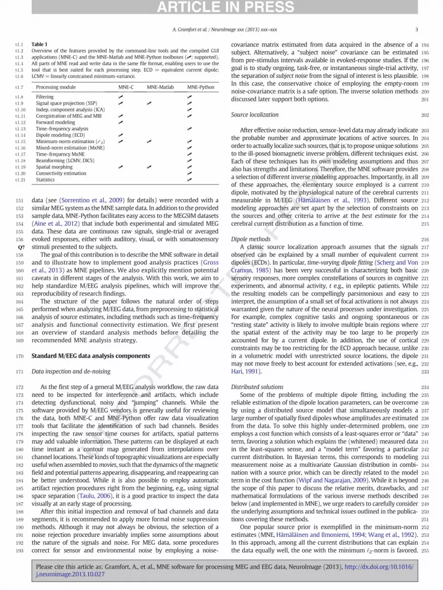
t1:2 Overview of the features provided by the command-line tools and the compiled GUIt1:3 applications (MNE-C) and the MNE-Matlab and MNE-Python toolboxes (✓: supported).t1:4 All parts of MNE read and write data in the same file format, enabling users to use thet1:5 tool that is best suited for each processing step. ECD = equivalent current dipole;t1:6 LCMV= linearly constrained minimum-variance.

t1:7 Processing module MNE-C MNE-Matlab MNE-Python

t1:8 Filtering ✓ ✓

t1:9 Signal space projection (SSP) ✓ ✓ ✓

t1:10 Indep. component analysis (ICA) ✓

t1:11 Coregistration of MEG and MRI ✓ ✓

t1:12 Forward modeling ✓

t1:13 Time–frequency analysis ✓

t1:14 Dipole modeling (ECD) ✓

t1:15 Minimum-norm estimation (ℓ2) ✓ ✓ ✓

t1:16 Mixed-norm estimation (MxNE) ✓

t1:17 Time–frequency MxNE ✓

t1:18 Beamforming (LCMV, DICS) ✓

t1:19 Spatial morphing ✓ ✓ ✓

t1:20 Connectivity estimation ✓

t1:21 Statistics ✓

3A. Gramfort et al. / NeuroImage xxx (2013) xxx–xxx

UNCO

RREC

data (see (Sorrentino et al., 2009) for details) were recorded with asimilarMEG systemas theMNE sample data. In addition to the providedsample data, MNE-Python facilitates easy access to the MEGSIM datasets(Aine et al., 2012) that include both experimental and simulated MEGdata. These data are continuous raw signals, single-trial or averagedevoked responses, either with auditory, visual, or with somatosensorystimuli presented to the subjects.

The goal of this contribution is to describe the MNE software in detailand to illustrate how to implement good analysis practices (Grosset al., 2013) as MNE pipelines. We also explicitly mention potentialcaveats in different stages of the analysis. With this work, we aim tohelp standardize M/EEG analysis pipelines, which will improve thereproducibility of research findings.

The structure of the paper follows the natural order of stepsperformed when analyzing M/EEG data, from preprocessing to statisticalanalysis of source estimates, including methods such as time–frequencyanalysis and functional connectivity estimation. We first presentan overview of standard analysis methods before detailing therecommended MNE analysis strategy.

Standard M/EEG data analysis components

Data inspection and de-noising

As the first step of a general M/EEG analysis workflow, the raw dataneed to be inspected for interference and artifacts, which includedetecting dysfunctional, noisy and “jumping” channels. While thesoftware provided by M/EEG vendors is generally useful for reviewingthe data, both MNE-C and MNE-Python offer raw data visualizationtools that facilitate the identification of such bad channels. Besidesinspecting the raw sensor time courses for artifacts, spatial patternsmay add valuable information. These patterns can be displayed at eachtime instant as a contour map generated from interpolations overchannel locations. These kinds of topographic visualizations are especiallyusefulwhen assembled tomovies, such that the dynamics of themagneticfield and potential patterns appearing, disappearing, and reappearing canbe better understood. While it is also possible to employ automaticartifact rejection procedures right from the beginning, e.g., using signalspace separation (Taulu, 2006), it is a good practice to inspect the datavisually at an early stage of processing.

After this initial inspection and removal of bad channels and datasegments, it is recommended to apply more formal noise suppressionmethods. Although it may not always be obvious, the selection of anoise rejection procedure invariably implies some assumptions aboutthe nature of the signals and noise. For MEG data, some procedurescorrect for sensor and environmental noise by employing a noise-


ED P

RO

OF

covariance matrix estimated from data acquired in the absence of asubject. Alternatively, a “subject noise” covariance can be estimatedfrom pre-stimulus intervals available in evoked-response studies. If thegoal is to study ongoing, task-free, or instantaneous single-trial activity,the separation of subject noise from the signal of interest is less plausible.In this case, the conservative choice of employing the empty-roomnoise-covariance matrix is a safe option. The inverse solution methodsdiscussed later support both options.

Source localization

After effective noise reduction, sensor-level datamay already indicatethe probable number and approximate locations of active sources. Inorder to actually localize such sources, that is, to propose unique solutionsto the ill-posed biomagnetic inverse problem, different techniques exist.Each of these techniques has its own modeling assumptions and thusalso has strengths and limitations. Therefore, the MNE software providesa selection of different inverse modeling approaches. Importantly, in allof these approaches, the elementary source employed is a currentdipole, motivated by the physiological nature of the cerebral currentsmeasurable in M/EEG (Hämäläinen et al., 1993). Different sourcemodeling approaches are set apart by the selection of constraints onthe sources and other criteria to arrive at the best estimate for thecerebral current distribution as a function of time.

Dipole methodsA classic source localization approach assumes that the signals

observed can be explained by a small number of equivalent currentdipoles (ECDs). In particular, time-varying dipole fitting (Scherg and VonCramon, 1985) has been very successful in characterizing both basicsensory responses, more complex constellations of sources in cognitiveexperiments, and abnormal activity, t e.g., in epileptic patients. Whilethe resulting models can be compellingly parsimonious and easy tointerpret, the assumption of a small set of focal activations is not alwayswarranted given the nature of the neural processes under investigation.For example, complex cognitive tasks and ongoing spontaneous or“resting state” activity is likely to involve multiple brain regions wherethe spatial extent of the activity may be too large to be properlyaccounted for by a current dipole. In addition, the use of corticalconstraints may be too restricting for the ECD approach because, unlikein a volumetric model with unrestricted source locations, the dipolemay not move freely to best account for extended activations (see, e.g.,Hari, 1991).

Distributed solutionsSome of the problems of multiple dipole fitting, including the

reliable estimation of the dipole location parameters, can be overcomeby using a distributed source model that simultaneously models alarge number of spatially fixed dipoles whose amplitudes are estimatedfrom the data. To solve this highly under-determined problem, oneemploys a cost function which consists of a least-squares error or “data”term, favoring a solution which explains the (whitened) measured datain the least-squares sense, and a “model term” favoring a particularcurrent distribution. In Bayesian terms, this corresponds to modelingmeasurement noise as a multivariate Gaussian distribution in combi-nation with a source prior, which can be directly related to the modelterm in the cost function (Wipf and Nagarajan, 2009). While it is beyondthe scope of this paper to discuss the relative merits, drawbacks, andmathematical formulations of the various inverse methods describedbelow (and implemented inMNE), we urge readers to carefully considerthe underlying assumptions and technical issues outlined in the publica-tions covering these methods.

One popular source prior is exemplified in the minimum-normestimates (MNE, Hämäläinen and Ilmoniemi, 1994; Wang et al., 1992).In this approach, among all the current distributions that can explainthe data equally well, the one with the minimum ‘2-norm is favored.




T

256

257

258

259

260

261

262

263

264

265

266

267

268

269

270

271

272

273

274

275

276

277

278

279

280

281

282

283

284

285

286

287

288

289

290

291

292

293

294

295

296

297

298

299

300

301

302

303

304

305

306

307

308

309

310

311

312

313

314

315

316

317

318

319

320

321

322

323

324

325

326Q8

327

328

329

330

331

332

333

334

335

336

337

338

339

340

341Q9

342

343

344

345

346

347

348

349

350

351

352

353

354

355

356

357

358

359

360

361

362

363

364

365

366

367

368

369

370

371

372

373

374

375

376

377

378

379

380

381

382


UNCO

RREC

This norm yields small, distributed estimates of cerebral currents(compared to e.g., an ‘1 norm, which favors a few, large-amplitudecurrents) to explain the observed sensor data. This MNE approach hassubsequently been refined to take into account cortical location andorientation constraints (Lin et al., 2006a), motivated by the neuro-physiological knowledge on the primary sources of the MEG and EEGsignals. Themost significant contributions to theM/EEG signals originatefrom postsynaptic currents in the pyramidal cells in the cortex and thenet direction of these currents is oriented perpendicular to the corticalsurface (Dale and Sereno, 1993). Incorporating this knowledge to themodel implies using individual anatomical information acquired withstructural magnetic resonance imaging (MRI). The current estimatescan then be constrained to the cortical mantle while the orientations ofthe currents can be further restricted to be perpendicular to the localcortical surface (Lin et al., 2006a). To quantify the statistical significanceof the current estimates, noise normalization techniques have beendeveloped (Dale et al., 2000; Pascual-Marqui, 2002) yielding adimensionless statistical score instead of dipole amplitudes in unitsof ampere-meter (Am). Mathematically, MNE is closely related toseveral other inversion approaches (Mosher et al., 2003).

A practical benefit of ‘2 solutions is that they yield physiologicallyplausible, temporally smooth estimates (without discontinuous‘jumps’). This comes at the cost of giving up some spatial precision. Toavoid smeared ‘2 estimates, sparsity-promoting priors such as ‘1-normprior may be desirable. Those generate more focal minimum-normsolutions, historically referred to as minimum-current estimates (MCEs)(Matsuura and Okabe, 1995; Uutela et al., 1999). Both assets, temporalsmoothness and focality, can also be combined using structured normssuch as the ‘21 mixed-norm (Gramfort et al., 2012; Ou et al., 2009).These norms can also be used to model non-stationary activations inthe time–frequency domain (Gramfort et al., 2013). The work of WipfandNagarajan (2009) offers a unifying view using a Bayesian perspectiveon some of the solvers implemented in the MNE software such as MNE,sLORETA, and the γ-MAP method.

BeamformersAnother class of distributed approaches, often referred to as

scanning methods, is exemplified by so-called adaptive beamformers,such as MUSIC (Mosher and Leahy, 1998), LCMV (Veen et al., 1997),SAM (Robinson and Vrba, 1998), and DICS (Gross et al., 2001). Thesemethods scan a grid of source locations, independently testing each ofthem for its contribution to the measured signal, similar to a radarbeam. Such techniques, some of which are implemented in the MNEsoftware, are almost exclusively computed on volumetric grids, asopposed to cortical surfaces commonly used with MNE. It should beemphasized, however, that even if the results are often referred to asimages they should be more appropriately called pseudo images, sincethey do not represent a distributed estimate of the cerebral electriccurrents that explain the measured M/EEG. Furthermore, the scanningtechniques are most often applied to MEG only, since their efficacydepends on the accuracy of the forward model, which is generally lessprecise for EEG than for MEG. Moreover, single-source beamformersyield erroneous localizations if several regions exhibit highly correlatedactivity, which is the case, e.g. for the bilateral auditory evoked responses.However, beamformers have been successfully employed in the analysisof ongoing spontaneous activity, where source correlations are in generalso low that the performance of a beamformer does not significantlydegrade (Gross et al., 2001). Also, alternative beamformer formulationscan alleviate the limitations of single-source beamformers (Wipf andNagarajan, 2007).

Statistics

Once activity estimates have been obtained,whether they are on thecortical surface or on a volume grid, a number of statistical measurescan be used to determine their significance. This statistical analysis


ED P

RO

OF

may consider, e.g., significance of activity with respect to a baseline, ordifferences across hemispheres, between conditions, between subjects,or between subject groups, e.g., patients and normal controls.

Several factors determine which statistical approach is the mostappropriate. Parametric methods are widely used and they build onunderlying assumptions (typically Gaussian) on the distribution of thedata to determine statistical significance, dynamic statistical parametricmapping (dSPM) estimates of significant activity being one prominentexample (Dale et al., 2000). When utilizing parametric methods, it isimportant to ensure that the underlyingmodel assumptions are satisfied,otherwise, the obtained results could be inaccurate (see (Pantazis et al.,2005) for discussion).

A more general class of statistical approaches comprises non-parametric methods, which do not rely on assumptions about thedistribution of the data. Permutation methods, in particular, exploit theexchangeability of conditions under the null hypothesis to estimate thenull distribution by resampling the data (Nichols and Holmes, 2002).

The appropriate statistical treatment depends on many factors, suchas whether the neural activity is represented as raw sensor signals,distributed source estimates, or parameters of equivalent current dipoles.Moreover, any given temporal waveform can be represented in terms offrequency content over an entire epoch, or that changes as a function oftime. Some analysis choices can increase the apparent dimensionality ofthe data considerably, and thus attention should be paid to the problemof multiple comparisons. This is a major reason that statistical analysismethods for M/EEG are evolving, and different forms of non-parametricapproaches (Nichols and Holmes, 2002; Pantazis et al., 2005), topologicalconsiderations (Maris and Oostenveld, 2007), and variance control(Ridgway et al., 2012) are being actively investigated. A comprehensivediscussion of the validity of these approaches is beyond the scope of thispaper. Our statistical approach outlined belowwill focus on the relativelynew non-parametric cluster-based statistical measures available inMNE, which provide the capability for statistical tests with minimalassumptions about the data distributions.

Functional connectivity

While the localization of activity using inverse modeling and succes-sive statistical tests can give us information on which brain regions areinvolved in a task and to what degree the amount of activity dependson other factors, e.g., experimental conditions, such an analysis typicallydoes not reveal how the brain regions relevant to the task are interrelated,apart possibly from the temporal sequence of activity in different regions.

Functional connectivity estimation methods analyze the relationshipbetween a number of time serieswith the goal of recovering the structureand properties of the network that describes the functional dependenciesbetween the underlying brain regions. Connectivity estimation inM/EEGis typically performed on non-averaged data (often after subtracting theevoked responses from the single trials) in either the sensor or the sourcespace. The latter requires the application of an inversemethod to obtain asource estimate for each trial, which is computationallymore demandingbut has the advantage that the connectivity can more directly be relatedto the underlying anatomy, which is difficult or even ambiguous forsensor-space connectivity estimates. Connectivity estimation in thesensor space also has the problem that the linear mixing introduced bythe forward propagation from cortical currents to the sensors, oftenreferred to as “spatial leakage” or, misleadingly, as “volume conduction”,can have a confounding effect on connectivity estimates. For connectivityanalysis, data can be segmented in consecutive epochs, e.g., 1 or 2s, afterfiltering. This has the benefit of using the same analysis pipeline used fortask-based data, which is particularly convenient as it allows anautomatic rejection of corrupted time segments using the epoch rejectionmechanisms.

MNE provides functions for connectivity estimation in both thesensor and source spaces. The supported methods are bivariate spectralmeasures, i.e., connectivity is estimated by analyzing pairs of time series,




T

383

384

385

386

387

388

389

390

391

392

393

394

395

396

397

398

399

400

401

402

403

404

405

406

407

408

409

410

411

412

413

414

415

416

417

418

419

420

421

422

423

424

425

426

427

428

429

430

431

432

433

434

435

436

437

438

439

440

441

442

443

444

445

446

447

448

449

450

451

452

453

454

455

456

457

458

459

460Q10

461

462

463

464

465

466

467

468

469

470

471

472

473

474

475

476

477

478

479

480

481

482

483

484

485

486

487

488

489

490

Fig. 2. Average power spectral density (PSD) of gradiometer channels estimated withWelch's method (Welch, 1967). The red region shows one standard deviation. One canclearly see the power line artifacts at 60, 120 and 180 Hz, that MNE can suppress withnotch filters.


UNCO

RREC

and they depend on the phase consistency across epochs between thetime series at a given frequency. Examples of such measures arecoherence, imaginary coherence (Nolte et al., 2004), and phase-lockingvalue (PLV) (Lachaux et al., 1999). The motivation for using imaginarycoherence and similar methods is that they discard or downweight thecontributions of zero-lag correlations, which are largely due to the spatialspread of the signals, both in the sensor space and in the source estimates(Schoffelen and Gross, 2009).

MNE supports severalmeasures that attempt to alleviate this problemof spurious connectivity due to zero-lag correlations. An alternative,complementary approach is the use of statistical tests to contrast theconnectivity obtained for different experimental conditions or groups ofsubjects. For seed-based connectivity estimation in the source space, thenon-parametric statistical tests implemented in MNE are ideally suitedfor this task as they control the familywise error rate and do not requireknowledge of the distribution under the null hypothesis, which is oftendifficult to obtain for connectivity measures. For example, this approachwas recently used to analyze long-range connectivity differences inpopulations with autism spectrum disorder (Khan et al., 2013). Allconnectivity measures in MNE can be computed either in the frequencyor the time–frequency domain. The use of time–frequency connectivityestimates is especially useful for event-related experiments as they enablethe investigation of connectivity changes over time relative to thestimulus onset.

It is important to note that even when using measures that cansuppress spurious zero-lag interactions and when contrasting betweenconditions, connectivity results should be interpreted with caution. Dueto the bivariate nature of the supported measures, there can be a largenumber of apparent connections due to a latent region connecting ordriving two regions that both contribute to the measured data.Multivariate connectivity measures, such as partial coherence (Grangerand Hatanaka, 1964), can alleviate this problem by analyzing theconnectivity between all regions simultaneously (cf. Schelter et al.,2006). However, multivariate measures are currently not supported inMNE, as connectivity estimation is one of the most recent additions toMNE. The inclusion of bivariate measures serves as a first step towardconnectivity estimation supportingmultivariate and effective connectivitymeasures (Friston, 1994), such as Wiener–Granger causality (Granger,1969; Wiener, 1956), which estimates directionality of influence. Whenanalyzing connectivity in source-space, it is also important to recognizethat the spatial spread of the inverse method can cause the connectivitybetween conditions to be significantly different even though there maynot be a significant difference in the actual connectivity. We refer toHaufe et al. (2012) for a recent simulation study that analyzes this issue.

Connectivity analysis in MNE has been implemented with processingefficiency in mind. For example, forward operator calculation distributescomputation acrossmultiple CPU cores. Filtering routines can operate inparallel across multiple CPU or GPU cores. Functional connectivityestimation uses a pipelined processing approach to reduce memoryconsumption, and the computational cost of time–frequency trans-forms has been reduced by taking advantage of linearity. Statisticalclustering routines and permutation methods take advantage of theunderlying connectivity structure, and use parallel processing tooptimize performance. This makes MNE ideally suited for the complex,computationally demanding tasks involved in processing sensor-spaceand source-space data.

The MNE way: Using MNE software for analysis

In this section, we provide a detailed description of the M/EEGanalysis steps supported by the MNE software. The description coversall components of MNE, i.e., MNE-C, MNE-Matlab, and MNE-Python.The outline of this section closely follows Table 1, which provides anoverview. Specifically, we cover preprocessing, discuss forward andinverse modeling, describe the surface based registration process (alsoknown as morphing) for group studies, explain the time–frequency


ED P

RO

OF

transforms implemented, discuss connectivity estimation in the sensorand source spaces, and finally describe the non-parametric statisticaltests offered.

Preprocessing

The MNE software contains graphical as well as command line-basedtools supporting data preprocessing. For visual inspection, MNE-Cprovides a raw data browser. MNE-Python can also visualize raw datatraces as well as show their rank and power spectrum using windowedfast Fourier transforms (FFTs) (Welch, 1967) (Fig. 2).

FilteringOften the signal of interest and interference occupy different frequen-

cy bands. MNE-C supports band-pass, low-pass, and high-pass filtering.The GUI also allows previewing the filtered data, so one can investigatethe impact of the filter on the signal. The Python toolbox extends theseoptions to include band-stop and notch filtering, optionally usingmulti-taper methods (Mitra and Bokil, 2008), which can be useful forsuppressing power-line artifactswhich are typically confined to narrowfrequency bands (Fig. 2). In addition, a filter-assembler function allowsfor tailoring custom filter kernels to the needs of particular datasets. Inorder not to introduce temporal shifts, all filters are implemented aszero-phase filters, which is achieved by applying the filters in theforward and backward directions. Still, care should be taken about theconsequences of filtering for subsequent analysis, e.g., in auto-regressive(AR) modeling commonly used for causality estimation (Barnett andSeth, 2011; Florin et al., 2010). Filters with infinite and finite impulseresponses (IIR and FIR, respectively) are both supported. To reduce thetime needed for the filtering operations, parallel processing is used toprocess several channels simultaneously. The FFTs required in the FIRfilter implementation can also be computed on the graphics processingunit (GPU),which can further reduce the execution time due to the highlyparallel architecture of a GPU.

Artifact rejectionAn important concern in preprocessing is to reduce interference

from endogenous (biological) and exogenous (environmental) sources.Artifact reduction strategies generally fall in two broad categories:exclusion of contaminated data segments and attenuation of artifactsby the use of signal-processing techniques (Gross et al., 2013). TheMNE “ecosystem” provides rich facilities supporting both approaches inconcert. When generating epochs, single epochs can be rejected basedon visual inspection using the raw data browser GUI, or automaticallyby defining thresholds for peak-to-peak amplitude and flat signaldetection (Fig. 3). The channels contributing to rejected epochs canalso be visualized to determine whether bad channels had been missedby visual inspection, or if noise rejectionmethods have been inadequate.




491

492

493

494

495

496

497

498

499Q11

500

501

502

503

504

505

506

507

508

509

510

511

512

513

514

515

516

517

518

519

520

521

522

523

524

525

526

527

528

529

530

531

532

533

534

535

536

537

538

539

540

541

Fig. 3. A sample evoked response (event-related fields on gradiometers) showing traces forindividual channels (bad channels are colored in red). Epochs with large peak-to-peaksignals as well as channels marked as bad can be discarded from further analyses.


Instead of simply excluding contaminated data from analysis, artifactscan sometimes be removed or significantly suppressed. For this purpose,MNE provides two complementary signal-processing approaches: signalspace projection (SSP; (Uusitalo and Ilmoniemi, 1997)) and independentcomponent analysis (ICA) (Jung et al., 2000).

T542

543

544

545

546

547

548

549

550

551

552

553

554

555

556

557

558

559

560

561

562

563

564

565

566

567

568
CO
RREC

Signal-space projection (SSP)The ideas behind SSP are to estimate an interference subspace and to

use a linear projection operator which is applied to the sensor data toremove the interference from the data. The underlying assumption ofSSP is that the noise subspace is orthogonal or at least sufficientlydifferent from the signal subspace of interest to avoid signal loss in theprojection. In practice, SSP is often determined by principal componentanalysis (PCA) of data with noise or prominent artifacts and then usingthe strongest principal components to construct the projection operator.With MEG data, the noise subspace can be estimated from empty-roomdata to suppress environmental artifacts. SSP operators can also beconstructed from time segments contaminated by endogenous artifactsinduced by electrical activity of the heart and or the eyes, i.e., themagneto/electrocardiogram (M/ECG) and magneto/electrooculogram(M/EOG), respectively. The latter includes both eye movements(saccades) and blinks. MNE-Python offers automated routines forheartbeat and blink detection. The Python visualization function allowsthe user to verify the output of this automatic procedure while theMNE-C graphical user interface (GUI) mne_browse_raw additionallyallows manual specification of time windows contaminated by artifacts.When applied to the data, SSP operators reduce the rank of the dataand also affect the spatial distribution of the signals. Therefore, projectionoperators have to be taken into account when computing the inversesolution. This implies that SSP operators that have been applied to thedata at any stage of the analysis pipeline cannot be discarded, which isthe reason why MNE stores them in the data files.

UN

Fig. 4. Trellis plot of 9 ICA components. The sources 0 to 5 are reordered by bivariate Pearson cwindow clearly resembles a cardiac signal. The time series 7 closely matches the EOG signal.


ED P

RO

OF

MNEmakes it easy to create and handle SSP operators. Projectors canbe manually assembled from within the raw data browser or auto-matically using commands and functions provided by the toolboxes.Once operators have been created and included in a measurement files,MNE defaults to handling the operators efficiently. That is, it will notmodify the original data immediately but instead apply the operatorsautomatically on demand as evoked responses and the inverse solutionsare computed. This also enables the user to explore the effects ofparticular SSPs and selectively drop projection vectors in cases wheresignal of interest is being lost. MNE can also display the effects of SSPson the strengths of the signal generated by a dipole at each cortical site.

Independent component analysis (ICA)Besides SSP, MNE supports identifying artifacts and sources using

temporal ICA. The assumption behind ICA is that the measured data arethe result of a linear combination of statistically independent time series,commonly named sources. ICA estimates amixingmatrix and source timeseries that are maximally non-Gaussian (kurtosis and skewness). Oncethese time series are uncovered, those reflecting, e.g., artifacts, can bedropped before reverting the mixing process. The ICA procedure in MNEis based on an implementation of the FastICA algorithm (Hyvärinen andOja, 2000) that is included with the scikit-learn package (Pedregosaet al., 2011). To reduce the computation time and to improve theunmixing performance, dimensionality reduction can be achieved usingthe randomized PCA algorithm (Martinsson et al., 2010).

To integrate data from different channel types that can have signalamplitudes orders of magnitude apart, the noise covariance matrixcan be used to whiten the data first. The ICA can be computed on eitherraw or epoched data. Also, one can either interactively select noise-freesources or perform a fully automated artifact removal. ICA sources canbe visualized using MNE functions that generate trellis plots (Beckeret al., 1996) (cf. Fig. 4).

The ICA sources can be exported as a raw data object and saved into aFIF file, hence allowing any sensor-space analysis to be performed on theICA time series: time–frequency analysis, raster plots, connectivity, orstatistics. For example, one can create epochs of ICA sources aroundartifact onsets and identify noisy ICA components by averaging.

MNE handles ICA in a similar manner as an SSP operator; the ICAdecomposition can be stored in a FIF file to be accessed later. Theunmixing matrix and the selection of the independent sources can thenbe reviewed and updated as required without having to modify orduplicate the original data. Once the matrices are available, and applyingthem to the data is about as fast as applying SSP projectors.

Combining SSP and ICAAlthough SSP and ICA both address the same family of problems, they

can be combined in useful ways. The orthonormal basis, as used in SSP,may give a plausible model of environmental noise, but not necessarilyso of highly skewed physiological artifact components for which ICA is

orrelation with the ECG channel. The first time series (index 0) displayed in the upper-left




T

569

570

571

572

573

574

575

576

577

578

579

580

581

582

583

584

585

586

587

588

589

590

591

592

593

594

595

596

597

598

599

600

601

602

603

604

605

606

607

608

609

610

611

612

613

614Q12

615

616

617

618

619

620

621

622

623

624

625

626

627

628

629630

631

632

633634Q13

635636637

638639640

641

642

643

644

645

646

647


REC

expected to achieve more accurate signal–artifact separation. Onthe other hand, the ICA model does not have an explicit noise term.Non-biological artifacts may not be that reliably modeled or detectedusing ICA, either due to their noise-like distribution, or for not meetingthe stationarity requirement in ICA. In practice, it is thereforerecommended to first apply empty-room SSP projections and then treatphysiological artifacts using ICA. Using MNE-Python covariance objects,optionally equipped with SSP vectors, ICA can take such projectionsinto account when modeling, transforming, and inverse-transformingdata.

Forward modeling

Computation of the magnetic field and the electric potentialThe physical relationship between cerebral electric currents and the

extracranial magnetic fields and scalp surface potentials measured byMEG and EEG is governed by Maxwell's equations. Importantly, thefrequencies of the neural electrical signals are sufficiently low to warrantthe use of the quasi-static approximation, i.e., the time-dependent termsinMaxwell's equations can be omitted (Hämäläinen et al., 1993; Plonsey,1969). Therefore, the MEG/EEG forward problem amounts to providingan accurate enough solution of the quasi-static version of Maxwell'sequations. The problem is further simplified by the fact that we canassume that the magnetic permeability of the head is that of the freespace and, therefore, only need to consider the distribution of electricalconductivity.

To solve the forward problem, one needs an approximation of thedistribution of the electrical and magnetic properties of the head, thespecifications of the elementary source model and the source space, thelocations of the EEG electrodes on the scalp and the configurations ofthe MEG sensors. The elementary source model in MNE is the currentdipole, and the electrical conductivity is assumed to be piecewiseconstant. With the latter approximation we can employ the boundaryelement model (BEM) (see, e.g., Mosher et al., 1999). MNE supportssingle- and three-compartment BEMs; the latter has to be employedwhen EEG data are present (Hämäläinen and Sarvas, 1989). The threecompartments need to be nested and correspond to the scalp, the skull,and the brain (cf. Fig. 5). MNE implements the BEM using the linearcollocationmethod (Mosher et al., 1999)with the isolated skull approach(Hämäläinen and Sarvas, 1989) to improve numerical precision.Alternative BEM formulations exist (Gramfort et al., 2010; Kybic et al.,2005; Mosher et al., 1999; Stenroos and Sarvas, 2012) but are notpresently implemented in MNE. The default electrical conductivities

UNCO

R

Fig. 5. Triangulated nested boundary surfaces used in the MNE BEM forward model: the inner susing the FreeSurfer package. By default, MNE employs 5120 triangles (2562 vertices) on each


ED P

RO

OF

used by MNE are 0.3 S/m for the brain and the scalp, and 0.006 S/m forthe skull, i.e., the conductivity of the skull is assumed to be 1/50 of thatof the brain and the scalp.

MNE relies on FreeSurfer for the automatic segmentation of the skulland the scalp surfaces. The segmentation can be done not only from thesame T1 MRI used for the FreeSurfer pipeline, which gives the corticalsurface segmentation, but also from flash MR images to improve thefidelity of skull segmentation. The triangulations used by MNE usuallyhave 5120 triangles for each of the three surfaces.

In addition to the BEM layers, the forward solver needs the propertiesof the sensors. For EEG, one only requires the electrode locations, and thusMNE supports all EEG systemswith a compatible file format (BrainVision,EDF, eXimia). For MEG, the locations, orientations and pick-up loopgeometries are needed for all sensors. AllmajorMEGvendors (Neuromag,CTF, 4D, KIT) are supported; the different MEG sensors (magnetometers,axial and planar gradiometers) are implemented with help of a “coildefinition” file, which contains the information about the individualpick-up coil geometries. Specifically, the output of the kth MEG sensor,bk, is approximated by the weighted sum

bks ¼XNk

p¼1

wkp B!

r!kp; r!s; es� �

� nkp ð1Þ

where B!

r! ; r!s; e!s

� �is the magnetic field at r! , generated by a unit

current dipole at r!s pointing to direction e, wkp is the scalar weights,r!kp is the locations within the pick-up coil loops comprising the MEGsensor, and nkp is the corresponding unit vectors normal to the planeof the pick-up loop. This equation states that the output of an MEGsensor is proportional to the sum of the magnetic fluxes threading thesensing coil loops of the flux transformer of a sensor. The integrationover the coil loops is performed numerically rather than analytically

using the integration points r!kp; nkp

n oand weights wkp. The winding

direction of the loops is taken into account in wkp.The coil definition file contains the numerical integration data for all

supported sensor types. Three different accuracies of integration areprovided: “minimal”, which usually ignores the finite size of the coilloops, “normal”, which provides sufficient accuracy for practical purposes,and “accurate”, which is the best available accuracy. In addition tothe primary sensors on the helmet, the compensation, or reference,magnetometers and gradiometers present in the CTF, 4D, and KITsystems are included in the forward model as well. If the data file

kull, the outer skull, and the scalp. The segmentations are obtained from T1 or Flash MRIssurface.




T

648

649

650

651

652

653

654

655

656

657

658

659

660

661

662

663

664

665

666

667

668

669

670Q14

671

672

673

674

675

676

677

678

679

680

681

682

683

684

685

686

687

688

689

690

691

692

693

694

695

696

697

698

699

700

701

702

703

704

705

706

707

708

709

710

711

712

713

714

715

716

717

718

719

720

721

722

723

724

725

726

727

728

729

730

731

732


RREC

to be processed indicates that “virtual gradiometers” have been createdusing the reference sensors, the forward calculation applies anautomatic correction for this noise rejection scheme.

The source spaceWhen working with distributed source models (see The MNE way:

UsingMNE software for analysis section) the locations of the elementarydipolar sources need to be specified a priori to compute the forwardoperator, also known as the gainmatrix. This ensemble of dipole locationsis called the source space. MNE can handle both volumetric and surfacesource spaces. For a volumetric source space one must specify the gridspacing, e.g., 5 or 7mmbetween neighboring points in 3D space, whereasfor a surface-based source space one must specify the surface and thesubsampling scheme. In this latter case, MNE by default uses the surfacebetween the gray and the white matters, although this can be changed,e.g. by using a FreeSurfer “mid” surface that is equidistant from white/gray matter interface and pial surface. Subsampling could be done bydecimating the surface mesh but preserving surface topology as wellas spacing and neighborhood information between vertices can bedifficult. Therefore, MNE uses a repeatedly subdivided icosahedron oroctahedron as the subsampling method. Once a subdivision step hasbeen accomplished, the resulting polyhedron is overlaid on the corticalsurface inflated to a sphere and the cortical vertices closest to thevertices of the the polyhedronare included to the source space. Forexample, an icosahedron subdivided 5 times, abbreviated ico-5, consistsof 10,242 locations per hemisphere, which leads to an average spacingof 3.1 mm between dipoles (assuming a surface area of 1000 cm2 perhemisphere). Such a source space is presented in Fig. 6. As there is noactual surface decimation, the cortical orientation used for orientation-constrained models is obtained by taking the normal of the high-resolution surface at the selected vertices. In addition, MNE also offersthe option to perform a numerical averaging of the normals over asmall patch around each selected vertex.

Coordinate system alignmentThe forward solver requires that the boundary-element surfaces,

the source space, and the sensor locations are defined in a commoncoordinate system. This is made possible by the co-registration step,which outputs the rigid-body transformation (translation and rotation)that relates the MRI coordinate system employed in FreeSurfer and theMEG “head” coordinate system, defined by the fiducial landmarks (twopre-auricular points and the nasion). In the beginning of each MEGstudy, the locations of the fiducial landmarks, the head-position indicator(HPI) coils, EEG electrodes, and a cloud of scalp surface points aredigitized and the MEG head coordinate system is set up. The position of

UNCO

Fig. 6. Cortical segmentation used for the source space in the distributedmodel withMNE. Left:hemisphere part of the source space (yellow dots), represented on the inflated surface of the rigper hemisphere with an average nearest-neighbor distance of 3.1mm.


ED P

RO

OF

the MEG sensor array in the MEG head coordinates is determined inthe beginning (and end) of each recording by feeding currents to theHPI coils and using the MEG sensor array to measure the resultingmagnetic fields. In addition, some systems offer the possibility forrecording the head position continuously during the actual acquisitionand compensation methods to bring all the data to a commoncoordinate frame (see, e.g., Taulu et al., 2005; Uutela et al., 2001).

As a result of acquiring the digitization and head position data andpossibly applying post-measurement correction for head movements,all information required for MEG–MRI co-registration is available inthe FIF files. An initial estimate for the coordinate transformation isobtained by manually identifying the fiducial landmarks from theMRI-based rendering of the head surface. This initial approximation isthen automatically refinedby using the iterative closest-point algorithm(Besl and McKay, 1992) which optimizes the transformation given therequirement that the digitized scalp surface points must be as close aspossible to the MRI-defined scalp. The accuracy of this step is particularlycrucial for precise source estimation (Hillebrand and Barnes, 2003). Theco-registration tools are available both in MNE-C and MNE-Python.

SummaryAs described above, the solution of the forward problem involves a

number of steps with a few parameters that have well-establisheddefault values. The forward computation pipeline in MNE is fullyautomatic thanks to the underlying FreeSurfer software. The onlymanualstep is the co-registration, which takes a couple of minutes and needs tobe done only once for each MEG session.

Inverse modeling

Although careful sensor-level data analysis can offer important insightinto the location and timing of neural activity, the accurate localizationof the underlying neural sources is of major interest for neuroscientificresearch. For this purpose, the MNE software implements severalmethods for solving the electromagnetic inverse problem using distrib-uted source spaces, either surface-based or volumetric. MNE employsthe same noise-covariance matrix to whiten the data and the forwardsolution consistently in all implemented source estimation methods.

For reconstructing the source current density, the MNE softwareimplements the minimum norm estimate (MNE), i.e., the Bayesianmaximum a posteriori (MAP) estimate with a Gaussian prior distributionon the source amplitudes (Dale and Sereno, 1993; Hämäläinen andIlmoniemi, 1984, 1994). In order to account for the depth localizationbias known forMNE, that is, the tendencyofMNEmethods to favor super-ficial sources, the MNE software allows to apply a depth-weighting

The pial (red) andwhitematter (green) surfaces overlaid on anMRI slice. Right: The right-ht hemisphere, was obtained by subdivision of an icosahedron leading to 10,242 locations




T

733

734

735

736

737

738

739

740

741

742

743

744

745Q15

746

747

748

749

750

751

752

753

754

755

756

757

758

759

760

761

762

763

764

765

766

767

768

769

770

771

772

773

774

775

776

777

778

779

780

781

782

783

784

785

786

787

788

789

790

791

792

793

794

795

796

797

798

799

800

801

802

803

804

805

806

807

808

809

810

811

812

813

814

815

816


REC

scheme based on scaling the source covariancematrix (Fuchs et al., 1999;Lin et al., 2006b). This approach is often referred to as the weightedminimum norm estimate (wMNE).

The MNE solution can be computed without restricting the sourceorientations.However, following the general assumption that theprimarysources of MEG and EEG signals are postsynaptic currents in the apicaldendrites of cortical pyramidal neurons, the net current can be assumedto be normal to the cortical mantle. MNE can constrain the dipoleorientations when a cortical surface source space is employed.

The first option is to fix the source orientations to be normal to theunderlying surface, which can be computed based either on a singlesource or on the statistics of a cortical surface patch surrounding thesource location. This is known as a fixed-orientation solution (Dale andSereno, 1993). Accordingly, there is an option in MNE software tocompute the forward solution for dipoles oriented normal to the corticalmantle only. However, it is recommended to always compute the gainmatrix for all dipole orientations because the depth weightingparameter for wMNE cannot be set correctly without this information(Lin et al., 2006b). Alternatively, the fixed orientation constraint can berelaxed (Lin et al., 2006a). In this loose orientation constraint approach,the variances of the source components oriented tangentially to thecortical surface are scaled by 0 b β b 1, where β=0 is equivalent to thefixed orientation constraint and β = 1 corresponds to free dipoleorientations. The parameter β=0 can also be set automatically and bemade location-dependent by using the cortical patch statistics, i.e., thevariance of the cortical normals within the patch corresponding to eachsource space point (Lin et al., 2006a) to determine β for each corticalsource site.

In addition to reconstructing the actual current density, the MNEsoftware includes two methods for computing noise-normalizedlinear inverse estimates. These methods, namely dynamic statisticalparameter mapping (dSPM) (Dale et al., 2000) and standardized low-resolution brain electromagnetic tomography (sLORETA) (Pascual-Marqui, 2002), transform the current density values into dimensionlessstatistical quantities, which help identify where the estimated currentdiffers significantly from baseline noise. Moreover, the noise-normalizedmethods reduce the location bias of the estimates. In particular, thetendency of the MNE to prefer superficial currents is reduced, and thewidth of the point-spread function becomes more uniform across thecortex (Dale et al., 2000). An example of a dSPM source estimate isshown in Fig. 7.

In order to include a priori information on the source locationcoming from other measurement modalities, the MNE software allows

UNCO

R

Fig. 7. Source localization of an auditory N100 component using dSPM. The regularizationparameter was set to correspond to SNR=3 in thewhitened data, source orientation hada loose constraint (β=0.2), and depth weighting was set to 0.8 (all three default values).


ED P

RO

OF

computing fMRI-guided linear inverse estimates (Dale et al., 2000).The fMRI weighting involves two steps. First, the fMRI activation mapis thresholded at a user-defined value to identify significant fMRIactivations. Thereafter, the elements of the source-covariance matrixcorresponding to sources being located in regions falling below thethreshold are scaled down by a user-defined factor (Liu et al., 1998). Itis important to note that the fMRI weighting has a strong influence onthe MNE solution, whereas the noise-normalized estimates are lessaffected.

As an addition to the linear inverse methods, theMNE software alsoincludes estimation of equivalent current dipoles (ECDs). At present,dipole fitting is limited to a single ECD at a single time point. The fittingprocedure is based on a four-step approach. First, an initial guess of theECD location is determined by an exhaustive search through a predefinedgrid. Thereafter, a Nelder–Mead simplex optimization is applied andthe risk of arriving at a local minimum is reduced by repeating theoptimization using the result of the first minimization as an initialguess; the best solution (highest goodness-of-fit) is retained. Finally,the ECD amplitude is computed.

All methods mentioned above can be applied as batch-modecommands or by using the interactive mne_analyze tool, a graphicaluser interface provided by the MNE-C code that can also be used forthe visual inspection of the source reconstruction results. Alternatively,snapshots and movies of the source reconstruction results can be savedfor inspection and processing with a batch-mode command. Pythonalso offers brain visualization capabilities through the PySurfer package(http://pysurfer.github.com). Both MNE-C and MNE-Python allow theuser to display source maps in a customizable fashion. MNE-Pythonextends some of these capabilities by making it much easier toautomate generation and annotation of figures via scripting of graphicalcalls.

In addition to the inversemethodsmentioned above, theMNE-Pythonpackage contains a set of imaging methods based on spatio-temporalsparse priors, which allow reconstruction of spatially sparse, i.e.,ECD-like source estimates with a distributed sourcemodel. These priorsare applied either in the time domain, e.g., the minimum currentestimate (MCE) (Matsuura and Okabe, 1995; Uutela et al., 1999), theγ-MAP estimate detailed in Wipf and Nagarajan (2009), and themixed norm estimate (MxNE) (Gramfort et al., 2012; Ou et al., 2009),or in the time–frequency domain, e.g., the time–frequency mixednorm estimate (TF-MxNE) (Gramfort et al., 2013) (Fig. 8). Furthermore,

Fig. 8. Source localization obtained with the time–frequency mixed-norm estimates(TF-MxNE) (Gramfort et al., 2013) for the right visual condition. The labels of the primaryand secondary visual cortices (V1 in red and V2 in yellow) estimated by FreeSurfer fromthe T1 MRI are overlaid on the cortical surface.


http://pysurfer.github.com



T

817

818

819

820

821

822

823

824

825

826

827

828

829

830

831

832

833

834

835

836

837

838

839

840

841

842

843

844

845

846

847

848

849

850

851

852

853

854

855

856

857

858

859

860

861

862

863

864

865

866

867

868

869

870

871

872

873

874

875

876

877

878

879

880

881

882

883

884

885

886

887

888

889

890

891

892

893

894

895

896

897


REC

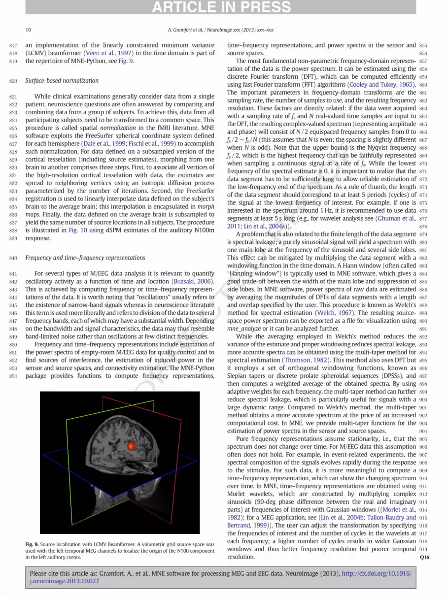
an implementation of the linearly constrained minimum variance(LCMV) beamformer (Veen et al., 1997) in the time domain is part ofthe repertoire of MNE-Python, see Fig. 9.

Surface-based normalization

While clinical examinations generally consider data from a singlepatient, neuroscience questions are often answered by comparing andcombining data from a group of subjects. To achieve this, data from allparticipating subjects need to be transformed to a common space. Thisprocedure is called spatial normalization in the fMRI literature. MNEsoftware exploits the FreeSurfer spherical coordinate system definedfor each hemisphere (Dale et al., 1999; Fischl et al., 1999) to accomplishsuch normalization. For data defined on a subsampled version of thecortical tesselation (including source estimates), morphing from onebrain to another comprises three steps. First, to associate all vertices ofthe high-resolution cortical tesselation with data, the estimates arespread to neighboring vertices using an isotropic diffusion processparameterized by the number of iterations. Second, the FreeSurferregistration is used to linearly interpolate data defined on the subject'sbrain to the average brain; this interpolation is encapsulated in morphmaps. Finally, the data defined on the average brain is subsampled toyield the same number of source locations in all subjects. The procedureis illustrated in Fig. 10 using dSPM estimates of the auditory N100mresponse.

Frequency and time–frequency representations

For several types of M/EEG data analysis it is relevant to quantifyoscillatory activity as a function of time and location (Buzsaki, 2006).This is achieved by computing frequency or time–frequency represen-tations of the data. It is worth noting that “oscillations” usually refers tothe existence of narrow-band signals whereas in neuroscience literaturethis term is usedmore liberally and refers to division of the data to severalfrequency bands, each ofwhichmay have a substantialwidth. Dependingon the bandwidth and signal characteristics, the data may thus resembleband-limited noise rather than oscillations at few distinct frequencies.

Frequency and time–frequency representations include estimation ofthe power spectra of empty-room M/EEG data for quality control and tofind sources of interference, the estimation of induced power in thesensor and source spaces, and connectivity estimation. The MNE-Pythonpackage provides functions to compute frequency representations,

UNCO

R 898

899

900

901

902

903

904

905

906

907

908

909

910

911

912

913

914

915

916

917

918

919

920Q16

Fig. 9. Source localization with LCMV Beamformer. A volumetric grid source space wasused with the left temporal MEG channels to localize the origin of the N100 componentin the left auditory cortex.


ED P

RO

OF

time–frequency representations, and power spectra in the sensor andsource spaces.

The most fundamental non-parametric frequency-domain represen-tation of the data is the power spectrum. It can be estimated using thediscrete Fourier transform (DFT), which can be computed efficientlyusing fast Fourier transform (FFT) algorithms (Cooley and Tukey, 1965).The important parameters in frequency-domain transforms are thesampling rate, the number of samples to use, and the resulting frequencyresolution. These factors are directly related: if the data were acquiredwith a sampling rate of fs and N real-valued time samples are input totheDFT, the resulting complex-valued spectrum(representing amplitudeand phase) will consist of N / 2 equispaced frequency samples from 0 tofs / 2− fs /N (this assumes that N is even; the spacing is slightly differentwhen N is odd). Note that the upper bound is the Nyqvist frequencyfs / 2, which is the highest frequency that can be faithfully representedwhen sampling a continuous signal at a rate of fs. While the lowestfrequency of the spectral estimate is 0, it is important to realize that thedata segment has to be sufficiently long to allow reliable estimation ofthe low-frequency end of the spectrum. As a rule of thumb, the lengthof the data segment should correspond to at least 5 periods (cycles) ofthe signal at the lowest frequency of interest. For example, if one isinterested in the spectrum around 1Hz, it is recommended to use datasegments at least 5 s long (e.g., for wavelet analysis see (Ghuman et al.,2011; Lin et al., 2004a)).

A problem that is also related to thefinite length of the data segmentis spectral leakage; a purely sinusoidal signal will yield a spectrumwithone main lobe at the frequency of the sinusoid and several side lobes.This effect can be mitigated by multiplying the data segment with awindowing function in the time domain. A Hann window (often called“Hanning window”) is typically used in MNE software, which gives agood trade-off between the width of the main lobe and suppression ofside lobes. In MNE software, power spectra of raw data are estimatedby averaging the magnitudes of DFTs of data segments with a lengthand overlap specified by the user. This procedure is known as Welch'smethod for spectral estimation (Welch, 1967). The resulting source-space power spectrum can be exported as a file for visualization usingmne_analyze or it can be analyzed further.

While the averaging employed in Welch's method reduces thevariance of the estimate and properwindowing reduces spectral leakage,more accurate spectra can be obtained using the multi-taper method forspectral estimation (Thomson, 1982). This method also uses DFT butit employs a set of orthogonal windowing functions, known asSlepian tapers or discrete prolate spheroidal sequences (DPSSs), andthen computes a weighted average of the obtained spectra. By usingadaptive weights for each frequency, themulti-taper method can furtherreduce spectral leakage, which is particularly useful for signals with alarge dynamic range. Compared to Welch's method, the multi-tapermethod obtains a more accurate spectrum at the price of an increasedcomputational cost. In MNE, we provide multi-taper functions for theestimation of power spectra in the sensor and source spaces.

Pure frequency representations assume stationarity, i.e., that thespectrum does not change over time. For M/EEG data this assumptionoften does not hold. For example, in event-related experiments, thespectral composition of the signals evolves rapidly during the responseto the stimulus. For such data, it is more meaningful to compute atime–frequency representation, which can show the changing spectrumover time. In MNE, time–frequency representations are obtained usingMorlet wavelets, which are constructed by multiplying complexsinusoids (90-deg phase difference between the real and imaginaryparts) at frequencies of interest with Gaussian windows ((Morlet et al.,1982); for a MEG application, see (Lin et al., 2004b; Tallon-Baudry andBertrand, 1999)). The user can adjust the transformation by specifyingthe frequencies of interest and the number of cycles in the wavelets ateach frequency; a higher number of cycles results in wider Gaussianwindows and thus better frequency resolution but poorer temporalresolution.




T

F

921

922

923

924

925

926

927

928

929

930

931

932

933

934

935

936

937

938

939

940

941

942

943

944

945

946

947

948

949

950

951

952

953

954

955

956

957

958

959

960

961

962

963

964

965

966

967

968

969

970

971

972

973

974

subject fsaveragemorphing

Fig. 10.Current estimates obtained in an individual subject can be remapped (morphed), i.e., normalized, to another cortical surface, such as that of the FreeSurfer average brain “fsaverage”shown here. The normalization is done separably for both hemispheres using a non-linear registration procedure defined on the sphere (Dale et al., 1999; Fischl et al., 1999). Here, theN100m auditory evoked response is localized using dSPM and then mapped to “fsaverage”.


RREC

We provide functions to compute time–frequency representations inboth the sensor and source spaces. Fig. 11 shows an example of aninduced power change, i.e., averaged power computed over an ensembleof epochs as opposed to evoked power obtained fromaveraged epochs, inresponse to electric stimulation of the left median nerve at wrist. Thisanalysis demonstrates a strong stimulus-induced power increase atabout 20Hz and starting about 500ms after the stimulus. Such reboundsof the oscillatory activity in the somatomotor system are well knowninduced responses (Hari and Salmelin, 1997).

When computing source-space power spectra or time–frequencyrepresentations with linear inverse operators (MNE, dSPM, sLORETA),MNE exploits the linearity of the operations to improve efficiencyas there are typically far more source points than sensors. This isaccomplished by computing the DFT in the sensor space, applying theinverse operator on the complex-valued result and taking the magnitudeat the source level.

Connectivity estimation

MNE can compute several bivariate connectivitymeasures in both thesensor and source spaces. The supported measures are all spectral, i.e.,they are based on estimates of cross spectral densities and dependingon the measure, power spectral densities. Currently, the connectivitymodule in MNE can compute coherence, coherency (complex-valuedcoherence), imaginary coherence (Nolte et al., 2004), phase-lockingvalue (PLV) (Lachaux et al., 1999), pairwise phase consistency (PPC)(Vinck et al., 2010), which is an unbiased estimate of PLV, phase lagindex (PLI) (Stam et al., 2007), and weighted phase lag index (WPLI)

UNCO 975

976

977

978

979

980

981

982

983

984

985

986

987

988

989

990

991

992

993

994

995

Fig. 11. Induced power change in the hand region along the right central sulcus. A total of111 epochs were used for the computation. The data in each epoch were transformed tothe source space using the dSPM method. The time–frequency representation wasobtained using 23Morlet wavelets with center frequencies 8–30Hz. The number of cyclesused increased linearly with the frequency: 4 cycles were used for 8 Hz and 15 cycles for30 Hz. Finally, the obtained time–frequency representation was averaged over a regionof interest in the source space, a.k.a. “label”, in the right central sulcus. The power wasbaseline-corrected to display percentage of variation (“3” means a 3-fold increase inpower compared to the pre-stimulus baseline).


ED P

RO

O(Vinck et al., 2011). In addition, the unbiased squared PLI and de-biasedsquared WPLI can be estimated (Vinck et al., 2011). Some methods, likeimaginary coherence and WPLI, and downweight zero-lag interactions,are therefore less affected by spurious interactions that exist in M/EEGsensor and source space data due to finite spatial resolution (Schoffelenand Gross, 2009). The use of the unbiased and de-biased versions of theestimators is recommended when connectivity is estimated based on asmall number of epochs. We refer to the above references for furtherdetails of each measure. The connectivity can be computed either in thefrequency or time–frequency domain using the appropriate transformsdescribed in the previous section.

To compute reliable connectivity estimates, the spectral estimationhas to be performed using tens or even hundreds of observations. InMNE, the observations are obtained by dividing the raw data into epochsusing event timings. For data that does not have events associated withthem, e.g., recordings of spontaneous brain activity, functions areprovided to generate events at fixed intervals, which enable connectivitycomputation for such data. To compute sensor-space connectivity, theepochs can be directly passed to the connectivity estimation routine. Bydefault, the connectivity measures between all N sensor time series arecomputed, which, due to symmetry, results in N(N− 1) / 2 connectivityestimates for all included frequency or time–frequency bins. For someexperiments, one may only be interested in the connectivity betweenselected pairs of time series, e.g., between a seed and all other timeseries. In MNE, the user can specify for which pairs of time series theconnectivity estimation should be performed.

The ability to compute the connectivity estimates for a subset ofconnections is especially useful when connectivity is estimated inthe source space, where the number of time series is much largerthan in the sensor space and all-to-all connectivity computation can beprohibitive. In order to estimate source-space connectivity, the epochdata are first projected to the source space bymeans of one of the inversemethods described earlier. Typically, either MNE, dSPM, sLORETA, orLCMV should be used as these methods work well for single-epochestimates where the SNR is low. Moreover, these linear methods arecomputationally efficient. It is important to note that spectral estimatesare meaningful only when the source estimates are signed. Therefore,when performing the inverse computation, the current componentoriented perpendicular to the cortical mantle must be used instead ofcombining the components for the three spatial dimensions, whichwould result in unsigned (magnitude) estimates. The obtained sourceestimates, one for each epoch, are then passed to the connectivity estima-tion routine.

As noted before, the large number of source-space time seriesmakesall-to-all connectivity estimation computationally very demanding. Anattractive option is therefore to reduce the number of time series andthus the computational demand by summarizing the source time serieswithin a set of cortical regions. We provide functions to do thisautomatically for cortical parcellations obtained by FreeSurfer, which




996

997

998

999

1000

1001

1002

1003

1004

1005

1006

1007

1008

1009

1010

1011

1012

1013

1014

1015

1016

1017

1018

1019

1020

1021

1022

1023

1024

1025

1026

1027

1028

1029

1030

1031

1032

1033

1034

1035

1036

1037

1038

1039

1040

1041

1042

1043

1044

1045

1046

1047

1048

1049


employs probabilistic atlases and cortical folding patterns for anautomated subject-specific segmentation of the cortex into anatomicalregions (Desikan et al., 2006; Destrieux et al., 2010; Fischl et al., 2004).The obtained set of summary time series can then be used as input tothe connectivity estimation. The association of time series with corticalregions simplifies the interpretation of results and it makes them directlycomparable across subjects since, due to the subject-specific parcellation,each time series corresponds to the same anatomical region in eachsubject. A result of such an analysis is illustrated in Fig. 12, where theconnectivity was computed for 68 cortical regions in the FreeSurfer“aparc” parcellation.

Due to the potentially large number of time series and epochs usedfor connectivity computation, an efficient implementation is important.InMNE, we reduce the computational cost by giving the user the optionto compute several connectivity measures at once, which reduces thecomputational demand as the spectral estimation only has to beperformed once. Furthermore, parallel processing enabled by modernmulti-core processors can be used to greatly reduce the computationtime.

Memory limitations are also important to consider. Assuming an oct-6source-space resolution (8196 vertices), 512 frequency points, anddouble-precision floating point representation, storing the multi-taperspectral estimate with 7 tapers for a single epoch requires 224 MB ofmemory. Therefore, a simplistic implementation which first computesthe spectral estimates leads to excessive memory requirements whenthe connectivity is computed over hundreds or even thousands of epochs.In MNE, we avoid this problem by using pipelined processing which isentirely hidden from the user; the user can write a linear script which

UNCO

RRECT

Fig. 12.Visualization of connectivity resulting from the presentations of a visual flash to the leftonset over 67 epochs. The inverse was computed using the dSPMmethod, with a source-spaceseries corresponding to the regions in the FreeSurfer “aparc” parcellation. All-to-all connectivi(Vinck et al., 2011) with multi-taper spectral estimation. Finally, the connectivity was visualize


PRO

OF

first extracts epochs, computes the inverse for each epoch, and thenpasses the result to the connectivity estimation function. However,internally, the actual computation is delayed in the sense that duringthe connectivity estimation, single epochs are extracted from the rawfile, the inverse is applied, and the spectra are estimated. However, forlinear inverses, higher computational efficiency is again achieved byautomatically applying the time–frequency or wavelet transforms insensor space before applying the inverse to the transformed data,which (due to linearity of the operations) results in the source-spacespectral estimates. This implementation leads to computationallyefficient connectivity estimation with memory requirements that areindependent of the number of epochs, which makes it possible toestimate source-space connectivity on desktop computers and laptopswith only a few GB of memory.

Statistics

The non-parametric statistical tests (Maris and Oostenveld, 2007)implemented in MNE are designed to provide a generic framework forstatistical analysis. This framework has been designed to be flexibleenough for the user to configure the clustering structure to reflect theunderlying topological features of interest. For example, the algorithmscan be used to cluster in time, which operates based on temporaladjacency alone, or in the time–frequency space, which operates byexamining temporally and spectrally contiguous regions. Both ofthese approaches would be appropriate for dipole fits or region-of-interest activations. Alternatively, clustering can be performed spatio-temporally, where the spatial adjacency of sensors or dipole locations

ED

visual hemifield. The connectivity was computed for−200–500ms relative to the stimulusresolution of 8196 vertices (oct-6). The source estimates were summarized into 68 time

ty was computed in the alpha band (8–13Hz) using the de-biased squared WPLI methodd as a circular graph using a connectivity visualization routine provided in MNE-Python.




T

1050

1051

1052

1053

1054Q17

1055

1056

1057

1058

1059

1060

1061

1062

1063

1064

1065

1066

1067

1068

1069

1070

1071

1072

1073

1074

1075

1076

1077

1078

1079

1080

1081

1082

1083

1084

1085

1086

1087

1088

1089

1090

1091

1092

1093

1094

1095

1096

1097

1098

1099

1100

1101

1102

1103

1104

1105

1106

1107Q18

1108

1109

1110

1111

1112

1113

1114

1115

1116

1117

1118

1119

1120

1121

1122

1123

1124

1125

1126

1127

1128

1129

1130

1131

1132

1133

1134

1135

1136

1137

1138

1139

1140

1141

1142

1143

1144

1145

1146

1147

1148

1149

1150

1151

1152

1153

1154

1155

1156

1157

1158

1159

1160

1161

1162

1163Q19

1164

1165

1166

1167

1168

1169

1170

1171

1172

1173

1174

1175

1176

1 http://www.ohloh.net/p/MNE.


UNCO

RREC

in the source space would be taken into account to identify spatially andtemporally contiguous regions of significant activity. Since this clusteringprocedure is independent of the statistic employed to determinesimilarity between the observations defining clusters, another importantimplication of the non-parametric cluster-statistics approach is thatarbitrary statistical functions can be used in combination with arbitrarycontrasts. Currently, MNE-Python directly supports one-sample t-tests,two-sample t-tests, one-way F-tests and two-way repeated-measuresANOVA for clustering–permutation tests. Additional statistical functionsare provided by other scientific and numerical Python packages, butalso user-defined functions can be included with ease as demonstratedin the MNE documentation.

Once significant clusters are obtained, functions are provided to helpsummarize them. The temporal center of mass is obtained byweightingeach time point by the number of significant vertices, while the spatialcenter of mass is obtained by weighting each vertex by the number ofsignificant time points. The spatial center of mass can then be easilytransformed into MNI Talairach coordinates for simple comparison toprevious neuroimaging studies (Larson and Lee, 2012).

Discussion

Data processing, such as M/EEG analysis, can be thought of as a chainor pipeline of operations, where each step has an impact on the results. Inthe preceding sections we have discussed particular choices made in theMNE software to proceed from preprocessing to advanced applicationssuch as statistics in the source space, including surface based registrationfor group studies, or connectivity measures between brain regions ofinterest.

MNE provides a few modules with graphical user interfaces (GUIs)that are valuable in inspecting and exploration of the data. However,we suggest that all of the processing should be done with scripts inwhich all parameters can be defined. The software has been designedwith this concept inmind. Data visualization GUIs are provided in Pythonfor every stage of processing (raw data, epoched data, evoked data, SSPeffects, time–frequency analysis, source estimates, cluster inspection,etc.), but provide very limited functionality for anything besidesinspecting the data. The idea is that the GUIs should allow users to becomfortable with (and understand) the effects of the chosen parameters,such as the baseline interval, regularization of MNE/dSPM/sLORETAinversion, and the amount of smoothing used for morphing the sourcetime courses. The downside of this approach is that MNE users areexpected to have basic programming skills to write shell, Matlab, orPython scripts. However, given the number of code snippets andexamples available on the MNE web site, a user typically ends up copy–pasting blocks of code to assemble their own pipeline. This choice canstill limit the user base and the impact of the software, however, thisapproach has clear benefits. First, our experience from analyzing severalM/EEG studies indicates that the processing pipeline needs to be tailoredfor each study. Even thoughmost pipelines follow the same logic includ-ingfiltering, epoching, averaging, etc., the number of options is large evenfor such standard steps. Scripting gives the flexibility to set those optionsand handle the requirements of different M/EEG studies.

Second, an analysis conducted with the help of scripts leads to morereproducible results. Indeed, reproducing a statistic or a figure can bedone by re-executing a script with the same input data. Scripting isalso away to prevent errors that usersmight introduce by inadvertentlychanging their behavior in the middle of the analysis, or because theyare running multiple studies simultaneously and for data from onesubject they use the parameters of another study. As the proceduresand steps chosen are accurately recorded in a script, the script is anefficient way to communicate one's research strategy to colleagues,who in return may provide more concise feedback targeting the levelof program code in addition to parameter descriptions from a report.This ultimately helps identify bugs and errors, thereby improving thequality of the particular research project. Nevertheless, it should be


ED P

RO

OF

pointed out that analysis steps requiring user interaction, e.g., time-varying dipole fits, which are presently not incorporated in MNE, canalso be made highly reproducible by proper training and scrutiny(Stenbacka et al., 2002).

Finally, studies that involve processing of data from dozens orhundreds of subjects aremade tractable via scripting. This is particularlyrelevant in an era of large-scale data analysis where massive cohorts ofsubjects may number more than a thousand, cf., the Human BrainProject or the Human Connectome Project (Van Essen et al., 2012).

Today neuroscientists from different academic disciplines spend anincreasing amount of timewriting software to process their experimentaldata. Data analysis is not limited to neuroimaging; nowadays almost allscientific data are processed by computers and software programs. Thepractical consequence of this is that the correctness of the scienceproduced relies on the quality of the software written (Dubois, 2005).The success of digital data analysis is made possible by high-qualitydata, by sophisticated numerical and mathematical methods, and lastbut not least by correct implementations. TheMNE software, in particularthe MNE-Python project, is developed and maintained to work towardhigh quality in terms of accuracy, efficiency and readability of the code.In order to measure and establish accuracy, the development processrequireswriting of unit and regression tests to ensure that the installationof the software is correct and that the results it gives match with resultspreviously obtained across multiple different computing platforms. Thistesting framework currently covers about 88% of the MNE-Python code.

Besides allowing users to track the stability and accuracy of thesoftware, this also makes it easier to incorporate new contributionsquickly without inadvertently breaking existing code.

By leveraging this open development approach, MNE has receivedmany contributions from the community. To control their quality, thepolicy in MNE development is that any code contribution must beread by two or more people, the author and one reviewer at minimum.This practice aims at establishing coding conventions that facilitate codereadability and bug fixing by users as has been demonstrated in otherprojects (Bhat and Nagappan, 2006; George and Williams, 2004;Marchenko et al., 2009). Importantly, the entire source code (includingthe full development history) ismade publicly available by a distributedversion control system. This makes it straightforward to keep track ofthe project's development and thus handle code changes in a way thatminimizes the risk of rendering existing scripts and analysis pipelinesinoperable. Finally, large parts of the source code are commentedusing inline documentation that allows for automatically building usermanuals in PDF and HTML formats. The Ohloh.net1 source code analysisproject attests that 36% of the source code consists of documentationand with this, MNE-Python's extent of documentation scores in theupper third of the Python projects publicly trackable. See Aruliah et al.(2012); Prlić and Procter (2012) for a more detailed presentation ofthe best practices for scientific software development beyond the fieldof neuroimaging.

TheMNE community not only employs amailing list ([email protected]; requires an approval to subscribe and post) as theprimary support channel, but also makes use of online services such asTwitter to announce new features and bug fixes, and GitHub to reportbugs and propose new features. GitHub is then used to follow theprogress made on bug fixes and added features.

As advocated above, scientific results should be easily reproducible.In addition, applying existing analysis methods on new data should bestraightforward as that fosters new scientific discoveries. In otherwords, analysis pipelines should be reusable across laboratories. Towardthat end, the MNE software package and Brainstorm have converged onmany aspects of the standard analysis pipeline, such as the imple-mentation of various noise-normalization methods. Continued sharingof methods and best practices facilitates research reproducibility.




http://www.ohloh.net/p/MNE



T

1177

1178

1179

1180

1181

1182

1183

1184

1185

1186

1187

1188

1189

1190

1191

1192

1193

1194

1195

1196

1197

1198

1199

1200

1201

1202

1203

1204

1205

1206

1207

1208

1209

1210Q20

1211

1212

1213

1214

1215

1216

1217

1218

1219

122012211222122312241225122612271228122912301231123212331234123512361237123812391240124112421243

1244124512461247124812491250125112521253125412551256125712581259126012611262126312641265126612671268126912701271127212731274127512761277127812791280128112821283128412851286128712881289Q211290129112921293129412951296129712981299130013011302130313041305130613071308130913101311131213131314131513161317131813191320132113221323132413251326132713281329


UNCO

RREC

In order tomaximize the impact of software, caremust be taken aboutthe license governing its use. The MNE-Python and MNE-Matlab codesare for this reason provided under the very permissive Open SourceBSD license. This license allows anybody to reuse and redistribute thiscode, even for commercial applications. The MNE-Matlab code is forexample redistributed with Brainstorm (Tadel et al., 2011), FieldTrip(Oostenveld et al., 2011), NutMeg (Dalal et al., 2011) and SPM (Litvaket al., 2011) to read and write FIF files.

Neuroimaging is a broad field encompassing static images, such asanatomical MRI as well as dynamic, functional data such M/EEG andfMRI. The MNE software relies on other packages such as FreeSurfer foranatomical MRI processing, and NiBabel (http://nipy.org/nibabel) forreading and writing images such as standard NIfTI files. Our ambition isnot to make MNE self-contained; the MNE package cannot and doesnot aim to do everything. MNE has its own scope and leverages thecapabilities of external software in the neuroimaging software ecosys-tem. Tighter integration with fMRI analysis pipelines could be facilitatedby NiPype (Gorgolewski et al., 2011) but is first made possible byadopting standards. That is why all data MNE produces are stored in FIFfile format which can be read and written by various software packages.The MNE-Python code also relies on core scientific libraries, namelyNumpy and Scipy (Milmann andAvaizis, 2011), andworkswith standarddata structures (Van der Walt et al., 2011) that are also used in mostscientific Python packages.

Good science requires not only good hypothesis and theories, creativeexperimental designs, and principled analysis methods, but also well-established data analysis tools and software. A scientific discovery is theend of a long chain, which will break at its weakest link. The MNEsoftware provides a solid foundation for reproducible scientificdiscoveries based M/EEG data. As the contributions to the MNE softwarepackage continue to grow, the MNE software suite should provideincreasing value to the neuroimaging community that has not onlyhelped determine its current form, but also continues to shape its future.

Acknowledgments

This work was supported by the National Institute of BiomedicalImaging and Bioengineering grants 5R01EB009048 and P41RR014075,National Institute on Deafness and Other Communication Disordersfellowship F32DC012456, and NSF awards 0958669 and 1042134. Thework of A.G. was partially supported by ERC-YStG-263584 and L.P. wassupported by the “aivoAALTO” program. M.L. was partially supportedby the Swiss National Science Foundation Early Postdoc. Mobilityfellowship 148485.

References

Aine, C., Sanfratello, L., Ranken, D., Best, E., MacArthur, J., Wallace, T., Gilliam, K., Donahue,C., Montao, R., Bryant, J., Scott, A., Stephen, J., 2012. MEG-SIM: a web portal for testingMEG analysismethods using realistic simulated and empirical data. Neuroinformatics10, 141–158.

Aruliah, D.A., Brown, C.T., Hong, N.P.C., Davis, M., Guy, R.T., Haddock, S.H.D., Huff, K.,Mitchell, I., Plumbley, M., Waugh, B., White, E.P., Wilson, G., Wilson, P., 2012. Bestpractices for scientific computing. Clin. Orthop. Relat. Res. abs/1210.0530.

Barnett, L., Seth, A.K., 2011. Behaviour of granger causality under filtering: theoreticalinvariance and practical application. J. Neurosci. Methods 201 (2), 404–419 (URLhttp://www.sciencedirect.com/science/article/pii/S01650 27011004687).

Becker, R.A., Cleveland, W.S., Shyu, M.-J., Kaluzny, S.P., et al., 1996. A Tour of TrellisGraphics. AT & T Bell Laboratories.

Besl, P., McKay, N.D., 1992. A method for registration of 3-d shapes. IEEE Trans. PatternAnal. Mach. Intell. 14 (2), 239–256.

Bhat, T., Nagappan, N., 2006. Evaluating the efficacy of test-driven development:industrial case studies. Proceedings of the 2006 ACM/IEEE international symposiumon Empirical software engineering. ACM, pp. 356–363.

Brookes, M.,Woolrich, M., Luckhoo, H., Price, D., Hale, J., Stephenson,M., Barnes, G., Smith,S., Morris, P., 2011. Investigating the electrophysiological basis of resting statenetworks using magnetoencephalography. Proc. Natl. Acad. Sci. U. S. A. 108 (40),16783–16788.

Buzsaki, G., 2006. Rhythms of the Brain, 1st edition. Oxford University Press, USA (Aug.).Cooley, J.W., Tukey, J.W., 1965. An algorithm for the machine calculation of complex

Fourier series. Math. Comput. 297–301.


ED P

RO

OF

Dalal, S.S., Zumer, J.M., Guggisberg, A.G., Trumpis, M., Wong, D.D.E., Sekihara, K.,Nagarajan, S.S., 2011. MEG/EEG source reconstruction, statistical evaluation, andvisualization with nutmeg. Comput. Intell. Neurosci. 2011.

Dale, A., Sereno, M., 1993. Improved localization of cortical activity by combining EEG andMEG with MRI cortical surface reconstruction: a linear approach. J. Cogn. Neurosci. 5(2), 162–176.

Dale, A., Fischl, B., Sereno, M., 1999. Cortical surface-based analysis I: segmentation andsurface reconstruction. NeuroImage 9, 179–194.

Dale, A., Liu, A., Fischl, B., Buckner, R., 2000. Dynamic statistical parametric mapping:combining fMRI and MEG for high-resolution imaging of cortical activity. Neuron 26,55–67.

Delorme, A., Makeig, S., 2004. EEGLAB: an open source toolbox for analysis of single-trialEEG dynamics including independent component analysis. J. Neurosci. Methods 134,9–21.

Delorme, A., Mullen, T., Kothe, C., Acar, Z.A., Bigdely-Shamlo, N., Vankov, A., Makeig, S.,2011. EEGLAB, SIFT, NFT, BCILAB, and ERICA: new tools for advanced EEG processing.Jan. Intell. Neurosci. http://dx.doi.org/10.1155/2011/130714 (10:10–10:10).

Desikan, R.S., Ségonne, F., Fischl, B., Quinn, B.T., Dickerson, B.C., Blacker, D., Buckner, R.L.,Dale, A.M., Maguire, R.P., Hyman, B.T., Albert, M., Killiany, R., 2006. An automatedlabeling system for subdividing the human cerebral cortex on MRI scans into gyralbased regions of interest. NeuroImage 31 (3), 968–980.

Destrieux, C., Fischl, B., Dale, A., Halgren, E., 2010. Automatic parcellation of human corticalgyri and sulci using standard anatomical nomenclature. NeuroImage 53 (1), 1.

Dubois, P., 2005. Maintaining correctness in scientific programs. Comput. Sci. Eng. 7 (3),80–85 (May).

Fischl, B., Sereno, M., Dale, A., 1999. Cortical surface-based analysis II: inflation, flattening,and a surface-based coordinate system. NeuroImage 9, 195–207.

Fischl, B., Van Der Kouwe, A., Destrieux, C., Halgren, E., Ségonne, F., Salat, D.H., Busa, E.,Seidman, L.J., Goldstein, J., Kennedy, D., Caviness, V., Makris, N., Rosen, B., Dale, A.,2004. Automatically parcellating the human cerebral cortex. Cereb. Cortex 14 (1),11–22.

Florin, E., Gross, J., Pfeifer, J., Fink, G.R., Timmermann, L., 2010. The effect of filtering ongranger causality based multivariate causality measures. NeuroImage 50 (2), 577–588(URL http://www.sciencedirect.com/science/article/pii/S10538 11909013391).

Fries, P., 2009. Neuronal gamma-band synchronization as a fundamental process incortical computation. Ann. Rev. Neurosci. 32, 209–224.

Friston, K.J., 1994. Functional and effective connectivity in neuroimaging: a synthesis.Hum. Brain Mapp. 2 (1–2), 56–78.

Fuchs, M., Wagner, M., Kohler, T., Wischmann, H.A., 1999. Linear and nonlinear currentdensity reconstructions. J. Clin. Neurophysiol. 16 (3), 267–295 (99353451 0736-0258 Journal Article Review Review, Tutorial).

George, B., Williams, L., 2004. A structured experiment of test-driven development. Inf.Softw. Technol. 46 (5), 337–342.

Ghuman, A.S., McDaniel, J.R., Martin, A., 2011. A wavelet-based method for measuringthe oscillatory dynamics of resting-state functional connectivity inMEG. NeuroImage(Jan.).

Gorgolewski, K., Burns, C.D., Madison, C., Clark, D., Halchenko, Y.O., Waskom, M.L., Ghosh,S.S., 2011. Nipype: a flexible, lightweight and extensible neuroimaging dataprocessing framework in python. Front. Neuroinform. 5 (13) (08).

Gramfort, A., Papadopoulo, T., Olivi, E., Clerc, M., 2010. OpenMEEG: opensource softwarefor quasistatic bioelectromagnetics. Biomed. Eng. Online 9 (1), 45.

Gramfort, A., Kowalski, M., Hämäläinen, M., 2012. Mixed-norm estimates for the M/EEG inverse problem using accelerated gradient methods. Phys. Med. Biol. 57(7), 1937–1961 (Mar).

Gramfort, A., Strohmeier, D., Haueisen, J., Hmlinen, M., Kowalski, M., 2013. Time–frequency mixed-norm estimates: sparse M/EEG imaging with non-stationary sourceactivations. NeuroImage 70, 410–422.

Granger, C., 1969. Investigating causal relations by econometric models and cross-spectralmethods. Econometrica 37 (3), 424–438.

Granger, C., Hatanaka, M., 1964. Spectral Analysis of Economic Time Series. PrincetonUniv. Press.

Gross, J., Kujala, J., Hämäläinen, M., Timmermann, L., 2001. Dynamic imaging of coherentsources: studying neural interactions in the human brain. Proc. Natl. Acad. Sci. 98 (2),694–699 (Jan).

Gross, J., Baillet, S., Barnes, G., Henson, R., Hillebrand, A., Jensen, O., Jerbi, K., Litvak, V.,Maess, B., Oostenveld, R., Parkkonen, L., Taylor, J., van Wassenhove, V., Wibral, M.,Schoffelen, J., 2013. Good practice for conducting and reporting MEG research.NeuroImage 65 (15), 349–363 (January).

Hämäläinen, M., Ilmoniemi, R., 1984. Interpreting magnetic fields of the brain: minimumnorm estimates. Tech. Rep. TKK-F-A559. Helsinki University of Technology.

Hämäläinen, M., Ilmoniemi, R., 1994. Interpreting magnetic fields of the brain: minimumnorm estimates. Med. Biol. Eng. Comput. 32 (1), 35–42 (Jan).

Hämäläinen, M.S., Sarvas, J., 1989. Realistic conductivity geometry model of the humanhead for interpretation of neuromagnetic data. IEEE Trans. Biomed. Eng. 36 (2),165–171 (Feb.).

Hämäläinen, M., Hari, R., Ilmoniemi, R., Knuutila, J., Lounasmaa, O., 1993. Magnetoen-cephalography — theory, instrumentation, and applications to noninvasive studiesof the working human brain. Rev. Mod. Phys. 65 (2), 413–497.

Hari, R., 1991. On brain's magnetic responses to sensory stimuli. J. Clin. Neurophysiol. 8(2), 157–169 (Apr.).

Hari, R., Salmelin, R., 1997. Human cortical oscillations: a neuromagnetic view throughthe skull. Jan. Trends Neurosci. 20 (1), 44–49 (PMID: 9004419).

Haufe, S., Nikulin, V.V., Müller, K.-R., Nolte, G., 2012. A critical assessment of connectivitymeasures for EEG data: a simulation study. NeuroImage 64, 120–133.

Hillebrand, A., Barnes, G.R., 2003. The use of anatomical constraints with MEGbeamformers. NeuroImage 20 (4), 2302–2313 (Dec.).


http://nipy.org/nibabel

http://dx.doi.org/10.1155/2011/130714



T

13301331133213331334Q2213351336133713381339134013411342134313441345134613471348Q23134913501351135213531354135513561357135813591360136113621363Q241364136513661367136813691370137113721373Q251374137513761377137813791380138113821383Q26138413851386138713881389139013911392139313941395139613971398Q271399140014011402140314041405140614071408140914101411

141214131414141514161417141814191420142114221423142414251426142714281429143014311432143314341435143614371438143914401441Q281442144314441445144614471448144914501451145214531454145514561457145814591460146114621463146414651466146714681469147014711472147314741475147614771478147914801481148214831484148514861487148814891490149114921493

1495


UNCO

RREC

Hipp, J.F., Hawellek, D.J., Corbetta, M., Siegel, M., Engel, A.K., 2012. Large-scale corticalcorrelation structure of spontaneous oscillatory activity. Nat. Neurosci. 15 (6),884–890 (Jun.).

Hyvärinen, A., Oja, E., 2000. Independent component analysis: algorithms and applications.Neural Netw.

Jung, T.-P., Makeig, S., Humphries, C., Lee, T.-W., Mckeown, M.J., Iragui, V., Sejnowski, T.J.,2000. Removing electroencephalographic artifacts by blind source separation.Psychophysiology 37, 163–178 (2).

Khan, S., Gramfort, A., Shetty, N.R., Kitzbichler, M.G., Ganesan, S., Moran, J.M., Lee, S.M.,Gabrieli, J.D., Tager-Flusberg, H.B., Joseph, R.M., et al., 2013. Local and long-rangefunctional connectivity is reduced in concert in autism spectrum disorders. Proc.Natl. Acad. Sci. 110 (8), 3107–3112.

Kybic, J., Clerc, M., Abboud, T., Faugeras, O., Keriven, R., Papadopoulo, T., 2005. A commonformalism for the integral formulations of the forward EEG problem. IEEE Trans. Med.Imaging 24 (1), 12–28.

Lachaux, J.-P., Rodriguez, E., Martinerie, J., Varela, F.J., et al., 1999. Measuring phasesynchrony in brain signals. Hum. Brain Mapp. 8 (4), 194–208.

Larson, E., Lee, A.K.C., 2012. The cortical dynamics underlying effective switching ofauditory spatial attention. Sep. NeuroImage (PMID: 22974974).

Lin, F.-H., Witzel, T., Hmlinen, M.S., Dale, A.M., Belliveau, J.W., Stufflebeam, S.M., 2004a.Spectral spatiotemporal imaging of cortical oscillations and interactions in thehuman brain. NeuroImage 23 (2), 582–595 (Sep.).

Lin, F.H., Witzel, T., Hamalainen, M.S., Dale, A.M., Belliveau, J.W., Stufflebeam, S.M., 2004b.Spectral spatiotemporal imaging of cortical oscillations and interactions in the humanbrain. NeuroImage 23 (2), 582–595 (1053-8119 (Print) Journal Article).

Lin, F., Belliveau, J., Dale, A., Hämäläinen, M., 2006a. Distributed current estimates usingcortical orientation constraints. Hum. Brain Mapp. 27, 1–13.

Lin, F.H., Witzel, T., Ahlfors, S.P., Stufflebeam, S.M., Belliveau, J.W., Hamalainen, M.S.,2006b. Assessing and improving the spatial accuracy in MEG source localization bydepth-weighted minimum-norm estimates. NeuroImage 31 (1), 160–171 (1053-8119(Print) Journal Article).

Litvak, V., Mattout, J., Kiebel, S., Phillips, C., Henson, R., Kilner, J., Barnes, G., Oostenveld, R.,Daunizeau, J., Flandin, G., Penny, W., Friston, K., 2011. EEG and MEG data analysis inSPM8. Comput. Intell. Neurosci.

Liu, A.K., Belliveau, J.W., Dale, A.M., 1998. Spatiotemporal imaging of human brain activityusing functional mri constrained magnetoencephalography data: Monte Carlosimulations. Proc. Natl. Acad. Sci. U. S. A. 95 (15), 8945–8950.

Marchenko, A., Abrahamsson, P., Ihme, T., 2009. Long-term effects of test-drivendevelopment a case study. Agile Processes in Software Engineering and ExtremeProgramming. Springer, pp. 13–22.

Maris, E., Oostenveld, R., 2007. Nonparametric statistical testing of EEG- and MEG-data.J. Neurosci. Methods 164 (1), 177–190 (Aug.).

Martinsson, P.-G., Rokhlin, V., Tygert, M., 2010. A randomized algorithm for thedecomposition of matrices. Appl. Comput. Harmon. Anal. (Feb.).

Matsuura, K., Okabe, Y., 1995. Selective minimum-norm solution of the biomagneticinverse problem. IEEE Trans. Biomed. Eng. 42 (6), 608–615 (June).

Milmann, K., Avaizis, M. (Eds.), 2011. Scientific Python. Computing in Science &Engineering, vol. 11. IEEE/AIP (March).

Mitra, P., Bokil, H., 2008. Observed Brain Dynamics. Oxford University Press, New York.Morlet, J., Arens, G., Fourgeau, E., Giard, D., 1982. Wave propagation and sampling theory:

part I: complex signal and scattering multilayered-part II: sampling theory and complexwaves. Geophysics 47, 203–236.

Mosher, J., Leahy, R., 1998. Recursive MUSIC: a framework for EEG and MEG sourcelocalization. IEEE Trans. Biomed. Eng. (Jan).

Mosher, J.C., Leahy, R.M., Lewis, P.S., 1999. EEG and MEG: forward solutions forinverse methods. IEEE Trans. Biomed. Eng. 46 (3), 245–259 (0018-9294 (Print)Journal Article).

Mosher, J., Baillet, S., Leahy, R., 2003. Equivalence of linear approaches in bioelectromagneticinverse solutions. 2003 IEEE Workshop on Statistical Signal Processing, pp. 294–297(Oct.).

Nichols, T.E., Holmes, A.P., 2002. Nonparametric permutation tests for functionalneuroimaging: a primer with examples. Jan. Hum. Brain Mapp. 15 (1), 1–25 (PMID:11747097).

Nolte, G., Bai, O., Wheaton, L., Mari, Z., Vorbach, S., Hallett, M., 2004. Identifying true braininteraction from EEG data using the imaginary part of coherency. Clin. Neurophysiol.115 (10), 2292–2307.

Oostenveld, R., Fries, P., Maris, E., Schoffelen, J.-M., 2011. Open source software foradvanced analysis of MEG, EEG, and invasive electrophysiological data. Comput.Intell. Neurosci.

Ou, W., Hämaläinen, M., Golland, P., 2009. A distributed spatio-temporal EEG/MEGinverse solver. NeuroImage 44 (3), 932–946 (Feb).

Pantazis, D., Nichols, T.E., Baillet, S., Leahy, R.M., 2005. A comparison of random fieldtheory and permutationmethods for the statistical analysis of MEG data. NeuroImage25 (2), 383–394 (Mar.).

Pascual-Marqui, R., 2002. Standardized low resolution brain electromagnetic tomography(sLORETA): technical details. Methods Find. Exp. Clin. Pharmacol. 24 (D), 5–12.

Pedregosa, F., Varoquaux, G., Gramfort, A., Michel, V., Thirion, B., Grisel, O., Blondel, M.,Prettenhofer, P., Weiss, R., Dubourg, V., Vanderplas, J., Passos, A., Cournapeau, D.,Brucher, M., Perrot, M., Duchesnay, E., 2011. Scikit-learn: machine learning in Python.J. Mach. Learn. Res. 12, 2825–2830.

Pérez, F., Granger, B.E., 2007. IPython: a system for interactive scientific computing. MayComput. Sci. Eng. 9 (3), 21–29 (URL http://ipython.org).

1494


ED P

RO

OF

Plonsey, R., 1969. Bioelectric Phenomena. McGraw-Hill, New York.Prlić, A., Procter, J.B., 2012. Ten simple rules for the open development of scientific

software. PLoS Comput. Biol. 8 (12).Ridgway, G.R., Litvak, V., Flandin, G., Friston, K.J., Penny, W.D., 2012. The problem of low

variance voxels in statistical parametric mapping; a new hat avoids a “haircut”.NeuroImage 59 (3), 2131–2141 (Feb.).

Robinson, S., Vrba, J., 1998. Functional neuroimaging by synthetic aperture magnetometry.In: Yoshimoto, T., Kotani, M., Kuriki, S., Karibe, H., Nakasato, N. (Eds.), Recent Advancesin Biomagnetism. Tohoku University Press, Sendai, Japan, pp. 302–305.

Schelter, B., Winterhalder, M., Timmer, J., 2006. Handbook of Time Series Analysis(Wiley.com).

Scherg, M., Von Cramon, D., 1985. Two bilateral sources of the late AEP as identified by aspatio-temporal dipole model. Electroencephalogr. Clin. Neurophysiol. 62 (1), 32–44(Jan.).

Schoffelen, J.-M., Gross, J., 2009. Source connectivity analysis with MEG and EEG. Hum.Brain Mapp. 30 (6), 1857–1865 (Jun.).

Sorrentino, A., Parkkonen, L., Pascarella, A., Campi, C., Piana, M., 2009. Dynamical MEGsource modeling with multi-target Bayesian filtering. Hum. Brain Mapp. 30 (6),1911–1921 (PMID: 19378276.URL http://www.ncbi.nlm.nih.gov/pubmed/19378276).

Stam, C.J., Nolte, G., Daffertshofer, A., 2007. Phase lag index: assessment of functionalconnectivity from multi channel EEG and MEG with diminished bias from commonsources. Hum. Brain Mapp. 28 (11), 1178–1193.

Stenbacka, L., Vanni, S., Uutela, K., Hari, R., 2002. Comparison of minimum currentestimate and dipole modeling in the analysis of simulated activity in the humanvisual cortices. NeuroImage 16 (4), 936–943 (Aug).

Stenroos, M., Sarvas, J., 2012. Bioelectromagnetic forward problem: isolated sourceapproach revis(it)ed. Phys. Med. Biol. 57 (11), 3517–3535 http://dx.doi.org/10.1088/0031-9155/57/11/3517 (Jun 7, Epub 2012 May 11).

Tadel, F., Baillet, S., Mosher, J.C., Pantazis, D., Leahy, R.M., 2011. Brainstorm: a user-friendlyapplication for MEG/EEG analysis. Comput. Intell. Neurosci.

Tallon-Baudry, C., Bertrand, O., 1999. Oscillatory gamma activity in humans and itsrole in object representation. Trends Cogn. Sci. 3 (4), 151–162 (1364-6613 Journalarticle).

Tallon-Baudry, C., Bertrand, O., Wienbruch, C., Ross, B., Pantev, C., 1997. Combined EEG andMEG recordings of visual 40Hz responses to illusory triangles in human. Neuroreport 5,1103–1107 (NA).

Taulu, S., 2006. Spatiotemporal signal space separation method for rejecting nearbyinterference in MEG measurements. Phys. Med. Biol. 51 (7), 1759–1769.

Taulu, S., Simola, J., Kajola, M., 2005. Applications of the signal space separation method.IEEE Trans. Signal Process. 53 (9), 3359–3372.

Thomson, D.J., 1982. Spectrum estimation and harmonic analysis. Proc. IEEE 70 (9),1055–1096.

Uusitalo, M., Ilmoniemi, R., 1997. Signal-space projection method for separating MEG orEEG into components. Med. Biol. Eng. Comput. 35 (2), 135–140.

Uutela, K., Hämäläinen, M., Somersalo, E., 1999. Visualization of magnetoencephalographicdata using minimum current estimates. NeuroImage 10, 173–180.

Uutela, K., Taulu, S., Hamalainen, M., 2001. Detecting and correcting for head movementsin neuromagnetic measurements. NeuroImage 14 (6), 1424–1431.

Van der Walt, S., Colbert, S., Varoquaux, G., 2011. The NumPy array: a structure forefficient numerical computation. Comput. Sci. Eng. 11.

Van Essen, D., Ugurbil, K., Auerbach, E., Barch, D., Behrens, T., Bucholz, R., Chang, A., Chen, L.,Corbetta, M., Curtiss, S., Della Penna, S., Feinberg, D., Glasser, M., Harel, N., Heath, A.,Larson-Prior, L., Marcus, D., Michalareas, G., Moeller, S., Oostenveld, R., Petersen, S.,Prior, F., Schlaggar, B., Smith, S., Snyder, A., Xu, J., Yacoub, E., 2012. The HumanConnectome Project: a data acquisition perspective. NeuroImage 62 (4), 2222–2231(Oct.).

Veen, B.V., Drongelen,W.V., Yuchtman,M., Suzuki, A., 1997. Localization of brain electricalactivity via linearly constrained minimum variance spatial filtering. IEEE Trans.Biomed. Eng. 44 (9), 867–880 (Jan).

Vinck, M., van Wingerden, M., Womelsdorf, T., Fries, P., Pennartz, C., 2010. The pairwisephase consistency: a bias-free measure of rhythmic neuronal synchronization.NeuroImage 51 (1), 112–122.

Vinck, M., Oostenveld, R., van Wingerden, M., Battaglia, F., Pennartz, C., 2011. An improvedindex of phase-synchronization for electrophysiological data in the presence ofvolume-conduction, noise and sample-size bias. NeuroImage 55 (4), 1548–1565.

Wang, J.-Z., Williamson, S.J., Kaufman, L., 1992. Magnetic source images determined by alead-field analysis: the unique minimum-norm least-squares estimation. IEEE Trans.Biomed. Eng. 39 (7), 665–675 (July).

Welch, P., 1967. The use of fast Fourier transform for the estimation of power spectra: amethod based on time averaging over short, modified periodograms. IEEE Trans.Audio Electroacoust. 15 (2), 70–73.

Wiener, N., 1956. The theory of prediction. ModernMathematics for Engineers.McGraw-Hill,New York.

Wipf, D., Nagarajan, S., 2007. Beamforming using the relevance vectormachine. Proceedingsof the 24th International Conference on Machine Learning. ICML'07. ACM, New York,NY, USA, pp. 1023–1030 (URL http://doi.acm.org/10.1145/1273496.1273625).

Wipf, D., Nagarajan, S., 2009. A unified Bayesian framework for MEG/EEG source imaging.NeuroImage 44 (3), 947–966 (Feb).

Wolters, C.H., Köstler, H., Möller, C., Härdtlein, J., Grasedyck, L., Hackbusch, W., 2007.Numerical mathematics of the subtraction method for the modeling of a currentdipole in EEG source reconstruction using finite element head models. SIAM J. Sci.Comput. 30 (1), 24–45.


http://dx.doi.org/10.1088/0031-9155/57/11/3517

http://dx.doi.org/10.1088/0031-9155/57/11/3517



Documents

MNE software for processing MEG and EEG data