Embed Size (px)
Citation preview
Modal Sequent Calculi
Labelled with Truth Values:
Completeness, Duality and Analyticity
P. Mateus1 A. Sernadas1 C. Sernadas1 L. Vigano2
1 CLC, Dep. Matematica, IST, Portugal2 ETH, Zurich, Switzerland
May 13, 2004
Abstract
Labelled sequent calculi are provided for a wide class of normal modalsystems using truth values as labels. The rules for formula constructorsare common to all modal systems. For each modal system, specific rulesfor truth values are provided that reflect the envisaged properties of the ac-cessibility relation. Both local and global reasoning are supported. Strongcompleteness is proved for a natural two-sorted algebraic semantics. As acorollary, strong completeness is also obtained over general Kripke seman-tics. A duality result is established between the category of sober algebrasand the category of general Kripke structures. A simple enrichment of theproposed sequent calculi is proved to be complete over standard Kripkestructures. The calculi are shown to be analytic in a useful sense.
Key words: modal logic, sequent calculus, labelled deduction.
AMS subject classification: 03B45, 03B22.
1 Introduction
Labelled deduction has been attracting much attention, namely within modallogic where it is natural to set up deduction systems using worlds as labels. Theidea of using worlds as labels is already found in [15]. More recently, the ideawas further explored in an attempt to produce modular calculi appropriatefor automation. Indeed, while for defining a Hilbert calculus for a specificmodal system one has to add just some extra axioms to the core calculus forsystem K, when setting up a sequent calculus (or a tableaux calculus, or anatural deduction calculus) for a specific modal system one has to start fromscratch (or almost). Usually, the rules needed for the modal system at hand arequite and subtly different from those of system K (see, for instance, [12, 20]).Labelled deduction opened a way out of this difficulty. With labelled deductionit is possible to keep the rules of the core calculus, adding for each modalsystem some extra rules about the labels (worlds), as proposed in, for instance,[10, 13, 4, 8, 19].

2
The idea of labelled deduction also appeared outside the context of modallogic, namely for finite many-valued logics where it is natural to use the truthvalues as labels [9, 3, 14].
More recently, labelled deduction has been applied in the context of researchon combining logics. Namely, as discussed in [16], combining deduction systemsrequires a sufficiently general notion of labelled deduction system in order tomake possible to combine, for instance, a natural deduction calculus for a modalsystem with a natural deduction calculus for a finitely many-valued logic. Tothis end, it is convenient to set up a deduction system with labels extractedfrom a suitable algebra of truth values.
In this paper, we adopt this novel approach, studying labelled sequent calculifor normal modal systems with labels extracted from an ordered algebra of truthvalues. The basic assertions are of the form θ ≤ ϕ expressing that truth valueθ is less than or equal to the denotation of formula ϕ. Observe that by atruth value we intend here a modal truth value that, in the context of Kripkesemantics, corresponds to a set of worlds.
The sequent calculi proposed in Section 2 share a common basis composedof: (i) structural rules; (ii) rules about the order among truth values; and(iii) rules for the formula constructors. The sequent calculus for each modalsystem is obtained by adding to this common basis specific rules imposing theunderlying properties of the accessibility relation. The calculi support bothglobal and local reasoning (corresponding to entailment over Kripke structuresand entailment over worlds, respectively). Section 2 ends with some metathe-orems not only interesting in themselves but also essential to the proof of thecompleteness results.
In Section 3, we start by proposing a new algebraic semantics involving twosorts (a sort for truth values and a sort for denotations of formulae). A quitegeneral completeness result is proved assuming very little about the sequentcalculus at hand (therefore, applicable outside the context of modal logic).Afterwards, we show how to move between general Kripke structures and suchalgebras in order to: (i) establish a characterization result showing that theproposed specific rules do characterize the frames with the intended propertiesof the accessibility relation; and (ii) obtain a completeness result over generalKripke structures as a corollary of the completeness theorem over algebraicsemantics.
Observe that the proposed labelled language is rich enough to express prop-erties of the accessibility relation that are not expressible by modal formu-lae (such as, irreflexivity, antisymmetry and asymmetry). Furthermore, weshow that the proposed specific rules characterize the envisaged properties evenamong general Kripke structures. This ability to deal with general Kripke se-mantics is a key advantage of the “truth values as labels” approach proposed inthis paper compared with the traditional “worlds as labels” approach. By theway, we also provide a simple enrichment of the language that leads to completecalculi over standard Kripke semantics.
Section 3 ends with a duality between the category of sober algebras and thecategory of general Kripke structures (with p-morphisms) and with a semanticproof of the analyticity of the proposed calculi (that is, we only need to apply

3
rules to known terms and formulae).The significance of the approach is further discussed in Section 4 where
interesting future developments are also mentioned, namely towards obtain-ing proof-theoretic results (like cut elimination), exploring the relationship tohybrid logic and moving out of the context of modal logic to tackle other logics.
2 Sequent calculi
2.1 Language
Assume given three sets ξi : i ∈ N, τi : i ∈ N and Γi : i ∈ N. The elementsof these sets are meta-variables of different kinds: each ξi may be replaced by a(simple) formula, each τi by a (truth value) term and each Γi by a (finite) bagof assertions as described below.
A signature is a tuple Σ = 〈C, O, X, Y, Z〉 where C = Ck : k ∈ N andO = Ok : k ∈ N such that each Ck and Ok is a countable set and ⊥,> ∈ O0
and X, Y, Z are countable sets. All these sets are assumed to be pair wisedisjoint. The elements of each Ck are known as (formula) constructors of arityk. Those of each Ok are known as (truth value) operators of arity k. Thoseof X are known as truth value unbound variables, while those of Y are knownas truth value bound variables. And those of Z are known as formula unboundvariables.
The sets X and Z are necessary because we need truth-value terms andformula terms to range over all possible values. Thus, an assignment will providea possible value for each x ∈ X and each z ∈ Z and the set of assignments coversall possible values. The set Y is required for a different reason. The truth valuebound variables in Y are needed in order to be able to universally quantify inthe inference rules.
The set F (Σ) of (schema) simple formulae over Σ is inductively definedas follows: (i) ξi ∈ F (Σ) for every i ∈ N; (ii) z ∈ F (Σ) for every z ∈ Z;(iii) c(ϕ1, . . . , ϕk) ∈ F (Σ) whenever c ∈ Ck and ϕ1, . . . , ϕk ∈ F (Σ). The setgF(Σ) of ground simple formulae is composed of the elements in F (Σ) withoutmeta-variables. The set cgF(Σ) of closed simple formulae is composed of theelements in gF(Σ) without variables.
The set T (Σ) of (schema) terms over Σ is inductively defined as follows:(i) τi ∈ T (Σ) for every i ∈ N; (ii) x ∈ T (Σ) for every x ∈ X; (iii) y ∈ T (Σ) forevery y ∈ Y ; (iv) o(θ1, . . . , θk) ∈ T (Σ) whenever o ∈ Ok and θ1, . . . , θk ∈ T (Σ);(v) #ϕ ∈ T (Σ) whenever ϕ ∈ F (Σ). The set gT(Σ) of ground terms is composedof the elements in T (Σ) without meta-variables. The set cgT(Σ) of closed termsis composed of the elements in gT(Σ) without variables.
The intended purpose of #ϕ is to say that we have a truth value term foreach formula.
The set A(Σ) of (schema) assertions over Σ is composed of the expressionsof the following six forms: (i) Ωθ and fθ (positive and negative truth value indi-visibility assertion, respectively) with θ ∈ T (Σ); (ii) θ v θ′ and θ 6v θ′ (positiveand negative truth value comparison assertion, respectively) with θ, θ′ ∈ T (Σ);(iii) θ ≤ ϕ and θ 6≤ ϕ (positive and negative labelled formula, respectively) with

4
θ ∈ T (Σ) and ϕ ∈ F (Σ). The set gA(Σ) of ground assertions is composed of theelements in A(Σ) without meta-variables. The set cgA(Σ) of closed assertionsis composed of the elements in gA(Σ) without variables.
The notion of conjugate δ of an assertion δ is introduced as follows: (i) Ωθis fθ; (ii) fθ is Ωθ; (iii) θ v θ′ is θ 6v θ′; (iv) θ 6v θ′ is θ v θ′; (v) θ ≤ ϕ is θ 6≤ ϕ;(vi) θ 6≤ ϕ is θ ≤ ϕ.
The intended meaning of Ωθ is to assert that a truth value term is atomic,that is, there is no term strictly smaller than it besides falsum. Clearly, themeaning of the conjugate fθ is to indicate that θ is not atomic. We do notconsider conjunctions and disjunctions of assertions because we do not needthem in the sequel, but they could easily be introduced. Instead, we work withsequents of assertions.
The set of (schema) labelled formulae over Σ is denoted by L(Σ). And theset of ground labelled formulae is denoted by gL(Σ).
A (schema) substitution over Σ is a map σ such that1: (i) σ(ξi) ∈ F (Σ);(ii) σ(τi) ∈ T (Σ); (iii) σ(Γi) ∈ Bf(A(Σ) ∪ Γi : i ∈ N). We denote the set of(schema) substitutions over Σ by Sbs(Σ).
A ground substitution over Σ is a schema substitution ρ such that: (i) ρ(ξi) ∈gF(Σ); (ii) ρ(τi) ∈ gT(Σ); (iii) ρ(Γi) ∈ Bf(gA(Σ)). We denote the set of groundsubstitutions over Σ by gSbs(Σ).
In what concern substitutions we also write Γiσ and Γiρ for σ(Γi) and ρ(Γi)respectively. The same applies to single formula and truth value terms.
2.2 Calculi
A sequent over a signature Σ is a pair s = 〈∆1, ∆2〉, written ∆1 → ∆2, where∆1, ∆2 ∈ Bf(A(Σ) ∪ Γi : i ∈ N). A sequent is said to be ground if it iswritten without meta-variables and it is said to be closed if furthermore it hasno variables.
The sequent calculi are composed by rules. As is standard for both labelledand unlabelled deduction calculi, the application of the rules is subject to con-straints. For example, in the Hilbert calculus for first-order logics we havethe axiom (∀x(ξ1 ⇒ ξ2) ⇒ (ξ1 ⇒ (∀xξ2))) provided that x does not occur freein ξ1. The meaning os such a proviso is to say that we only allow (ground)substitutions of the axiom where ξ1 is mapped to a formula ϕ where x doesnot occur free in ϕ. Hence a proviso can be looked upon as a set of allowedsubstitutions.
A (local) proviso over Σ is a map π : gSbs(Σ) → 0, 1. The unit provisoup is as follows: up(ρ) = 1 for every ρ ∈ gSbs(Σ). The zero proviso zp is asfollows: zp(ρ) = 0 for every ρ ∈ gSbs(Σ).
Given two provisos π, π′, their intersection is the proviso (π ∩ π′) such that(π ∩ π′)(ρ) = π(ρ)× π′(ρ). And we say that π ⊆ π′ when π(ρ) ≤ π′(ρ) for eachground substitution ρ. Therefore, a proviso π is included in a proviso π′ ifthe latter allows more ground substitutions than the former.
1Given a set U , we denote by BfU the set of all finite bags (multisets) of elements in U .

5
Given a schema substitution σ and a proviso π, the proviso (πσ) is as follows:(πσ)(ρ) = π(σρ) for every ρ ∈ gSbs(Σ).
Observe that, for every proviso π and ground substitution ρ, the proviso(πρ) is either up or zp.
A rule over Σ is a triple r = 〈s1, . . . , sp, s, π〉, written
s1 . . . sp
sC π ,
where s1, . . . , sp, s are sequents over Σ and π is a proviso over Σ. When π isup, the rule may be written
s1 . . . sp
s.
Given a sequent s = 〈∆1, ∆2〉 and a substitution σ both over Σ, we denoteby sσ the instance 〈∆1σ,∆2σ〉 of s by σ. Given a rule r and a substitution σboth over Σ, we denote by rσ the instance
s1σ . . . spσ
sσC πσ
of r by σ.A (sequent) calculus is a pair C = 〈Σ,R〉 where Σ is a signature and R is a
finite set of rules over Σ.Within the context of a sequent calculus C, we say that a sequent s′ is
derived from a set S of sequents with proviso π, written S `C s′ C π, if there isa sequence 〈d1, π1〉, . . . , 〈dn, πn〉 such that:
• d1 is s′ and π ⊆ π1;
• for every i = 1, . . . , n:
1. either di ∈ S and πi is up;
2. or there is an assertion that occurs in both sides of di and πi is up;
3. or there are r ∈ R, σ ∈ Sbs(Σ), p ∈ N and i1, . . . , ip ∈ i + 1, . . . , nsuch that
rσ =di1 . . . dip
diC π′
and πi = π′ ∩ πi1 ∩ · · · ∩ πip .
When the proviso π is up, we may write S `C s′. And we may write `C swhen the set of premises is empty. Furthermore, when the signature is obviousfrom the context we may write `R instead of `C . In derivations we justify 1by hyp (hypothesis), 2 by ax (axiom) and 3 by r[σ] : i1, . . . , ip.
Following [6, 1], we choose to display rules from premises to conclusions,and derivations starting from the conclusion since this simplifies their reading,as is illustrated by the example derivations below.
The derivation sequence 〈d1, π1〉, . . . , 〈dn, πn〉 is said to be sober if, for eachi = 2, . . . , n, i appears in the justification of some dj such that j < i. Itis straightforward to set up an algorithm to make sober any given derivation

6
sequence. It is also simple to set up an algorithm for extracting the traditionalderivation tree from any given sober derivation sequence.
When making proofs, we may write d1, . . . , dn for the derivation sequence〈d1,up〉, . . . , 〈dn,up〉.
Derivation establishes a finitary consequence operator for ground sequentsthanks to the following result:
Proposition 2.1 For any sequent calculus C:Projective If S `C s′ C π and π′ ⊆ π then S `C s′ C π′.
Finitary If S `C s′ C π then there is a finite S1 ⊆ S such that S1 `C s′ C π.
Extensive S `C s C up for each sequent s ∈ S.
Monotonic If S ⊆ S1 and S `C s′ C π then S1 `C s′ C π.
Idempotent If S1 `C s C πs for each s in a finite set S of sequents andS `C s′ C π then S1 `C s′ C π ∩ (
⋂
s∈S
πs).
The following result is also straightforward to prove (by induction on thelength of the derivation).
Proposition 2.2 For any sequent calculus C = 〈Σ,R〉 and substitution σ overΣ, if S `C s′ C π with derivation sequence 〈d1, π1〉, . . . , 〈dn, πn〉 then Sσ `Cs′σ C πσ with derivation sequence 〈d1σ, π1σ〉, . . . , 〈dnσ, πnσ〉.
2.3 Structural rules
A sequent calculus C = 〈Σ,R〉 is said to be structural if R contains the followingweakening, contraction, conjugation and cut rules:
LwΩ Γ1→Γ2Ωτ1,Γ1→Γ2
RwΩ Γ1→Γ2Γ1→Γ2,Ωτ1
LwT Γ1→Γ2τ1vτ2,Γ1→Γ2
RwT Γ1→Γ2Γ1→Γ2,τ1vτ2
LwF Γ1→Γ2τ1≤ξ1,Γ1→Γ2
RwF Γ1→Γ2Γ1→Γ2,τ1≤ξ1
LcT τ1vτ2,τ1vτ2,Γ1→Γ2
τ1vτ2,Γ1→Γ2RcT Γ1→Γ2,τ1vτ2,τ1vτ2
Γ1→Γ2,τ1vτ2
LcF τ1≤ξ1,τ1≤ξ1,Γ1→Γ2
τ1≤ξ1,Γ1→Γ2RcF Γ1→Γ2,τ1≤ξ1,τ1≤ξ1
Γ1→Γ2,τ1≤ξ1
LxiΩ Γ1→Γ2,Ωτ1fτ1,Γ1→Γ2
RxiΩ Ωτ1,Γ1→Γ2
Γ1→Γ2,fτ1
LxiT Γ1→Γ2,τ1vτ2τ1 6vτ2,Γ1→Γ2
RxiT τ1vτ2,Γ1→Γ2
Γ1→Γ2,τ1 6vτ2
LxiF Γ1→Γ2,τ1≤ξ1τ1 6≤ξ1,Γ1→Γ2
RxiF τ1≤ξ1,Γ1→Γ2
Γ1→Γ2,τ1 6≤ξ1
LxeΩ Γ1→Γ2,fτ1Ωτ1,Γ1→Γ2
RxeΩ fτ1,Γ1→Γ2
Γ1→Γ2,Ωτ1
LxeT Γ1→Γ2,τ1 6vτ2τ1vτ2,Γ1→Γ2
RxeT τ1 6vτ2,Γ1→Γ2
Γ1→Γ2,τ1vτ2
LxeF Γ1→Γ2,τ1 6≤ξ1τ1≤ξ1,Γ1→Γ2
RxeF τ1 6≤ξ1,Γ1→Γ2
Γ1→Γ2,τ1≤ξ1
cutT Γ1→Γ2,τ1vτ2 τ1vτ2,Γ1→Γ2
Γ1→Γ2cutF Γ1→Γ2,τ1≤ξ1 τ1≤ξ1,Γ1→Γ2
Γ1→Γ2

7
The rules above are known as structural rules. These structural rules arethe usual ones in sequent calculi plus those needed to deal with conjugates.The introduction of disjunction and conjunction of assertions would lead to theexpected left and right rules. Other rules that may be present in the sequentcalculus at hand are known as proper rules.
2.4 Order rules
Before proceeding, we need to introduce the following provisos:
• (τk : y)(ρ) = 1 iff ρ(τk) ∈ Y ;
• (τk 6∈ ∆)(ρ) = 1 iff ρ(τk) does not occur in ∆ρ.
The first proviso states that we only allow ground substitutions where τk isreplaced by a truth value bound variable. The second proviso indicates that weonly allow a substitution ρ if τk is replaced by a truth value not occurring inthe bag ∆ρ.
A structural sequent calculus C = 〈Σ,R〉 is said to be an order sequentcalculus if it contains the following additional order rules:
L# τ1≤ξ1,Γ1→Γ2
τ1v#ξ1,Γ1→Γ2R# Γ1→Γ2,τ1≤ξ1
Γ1→Γ2,τ1v#ξ1
⊥T Γ1→Γ2,⊥vτ1⊥F Γ1→Γ2,⊥≤ξ1
Ω⊥ Γ1→Γ2,Ωτ1Γ1→Γ2,τ1 6v⊥ > Γ1→Γ2,τ1v>
Ω> Ωτ1,Γ1→Γ2,τ1≤ξ1Γ1→Γ2,>≤ξ1
C τ1 : y, τ1 /∈ Γ1, Γ2
Ω Γ1→Γ2,τ1 6v⊥ Ωτ2,τ2vτ1,Γ1→Γ2,τ1vτ2Γ1→Γ2,Ωτ1
C τ2 : y, τ2 /∈ τ1, Γ1, Γ2
cons Γ1→Γ2,>6v⊥ ref Γ1→Γ2,τ1vτ1
transT Γ1→Γ2,τ1vτ2 Γ1→Γ2,τ2vτ3Γ1→Γ2,τ1vτ3
transF Γ1→Γ2,τ1vτ2 Γ1→Γ2,τ2≤ξ1Γ1→Γ2,τ1≤ξ1
Lasym Ωτ1,Ωτ2,τ1vτ2,Γ1→Γ2
Ωτ1,Ωτ2,τ2vτ1,Γ1→Γ2Rasym Ωτ1,Ωτ2,Γ1→Γ2,τ1vτ2
Ωτ1,Ωτ2,Γ1→Γ2,τ2vτ1
LgenT Ωτ2,τ2vτ3,Γ1→Γ2 Ωτ2,Γ1→Γ2,τ2vτ1 τ1vτ3,Γ1→Γ2,Ωτ2τ1vτ3,Γ1→Γ2
RgenT Ωτ2,τ2vτ1,Γ1→Γ2,τ2vτ3Γ1→Γ2,τ1vτ3
C τ2 : y, τ2 6∈ τ1, τ3, Γ1, Γ2
LgenF Ωτ2,τ2≤ξ1,Γ1→Γ2 Ωτ2,Γ1→Γ2,τ2vτ1 τ1≤ξ1,Γ1→Γ2,Ωτ2τ1≤ξ1,Γ1→Γ2
RgenF Ωτ2,τ2vτ1,Γ1→Γ2,τ2≤ξ1Γ1→Γ2,τ1≤ξ1
C τ2 : y, τ2 6∈ τ1, Γ1, Γ2
These rules impose intended meanings to the basic assertions that shouldbe obvious. But, it is worthwhile to note that if Ωt holds then t is intended todenote an atomic truth value (where a formula either holds or does not hold).
It is also worthwhile to explain the rules RgenF and LgenF. The rule RgenFindicates that if the value of τ2 is less than or equal to the value of ξ1 for allatomic τ2 included in τ1, then τ1 is less than or equal to the value of ξ1. We

8
also impose that τ2 is fresh so that the universal quantifier does not captureother variables namely those in τ1, Γ1, Γ2. The rule LgenF can be interpretedas follows: assuming that we have τ1 ≤ ξ1 and Γ1 in order to show that we haveγ2 for some γ2 ∈ Γ2 it is enough to show that there is an element τ2 such that
• τ2 is atomic (premise τ1 ≤ ξ1, Γ1 → Γ2, Ωτ2);
• τ2 v τ1 (premise Ωτ2,Γ1 → Γ2, τ2 v τ1);
• from τ2 ≤ ξ1 we have γ2 for some γ2 ∈ Γ2 (premise Ωτ2, τ2 ≤ ξ1, Γ1 → Γ2).
Observe also that this set of rules, although convenient, is by no meansminimal. For instance, rules L# and R# allow the derivation of the F rulesfrom the corresponding T rules. Moreover, rule Ω> is derived from RgenT. Notealso that not all of these rules are needed for obtaining later on the completenessresult over Kripke semantics (Theorem 3.25). Indeed, rules ref and asym areonly needed for establishing the duality between the algebraic semantics andthe Kripke semantics (see Subsection 3.4).
Note that the provisos used above do not change value when the contextof the rule at hand is enriched with closed assertions. More precisely, a rule issaid to be endowed with a persistent proviso if its proviso does not change valuewhen the context of the rule is enriched with a closed assertion.
For example, consider the rule RgenF. The context of the rule is Γ1 andΓ2, that is the bags of assertions in the conclusion of the rule. Note that if wechange the context by adding a closed assertion either to Γ1 or Γ2, the resultingproviso will allow precisely the same substitutions.
More generally, any rule with a “fresh bound variable” proviso like τ2 :y∩τ2 /∈ τ1, Γ1, Γ2 is endowed with a persistent proviso. Indeed, for every groundsubstitution ρ, it holds (τ2 : y∩τ2 /∈ τ1, Γ1, Γ2)(ρ) = (τ2 : y∩τ2 /∈ τ1, Γ1, Γ2, δ)(ρ)as long as δ is closed. Clearly, every rule endowed with the unit proviso up(which is omitted) is also endowed with a persistent proviso.
Therefore, according to this definition, the order rules above are endowedwith persistent provisos.
2.5 Modal system K specific rules
We now proceed to define the sequent calculus CK = 〈Σk,RK〉 for modal systemK. The modal signature ΣK = 〈C, O,X, Y, Z〉 is as follows:
• C0 = f , t ∪ pi : i ∈ N;• C1 = ¬,¤,♦;• C2 = ∧,∨,⇒;• Ck = ∅ for k ≥ 3;
• O0 = ⊥,>;• O1 = I,N;

9
• O2 = lb;• Ok = ∅ for k ≥ 3;
• X = xi : i ∈ N;• Y = yi : i ∈ N;• Z = zi : i ∈ N.Besides the structural and order rules introduced above, RK contains the
following specific rules:
I Γ1→Γ2,I(τ1)vτ1ΩI Γ1→Γ2,τ1 6v⊥
Γ1→Γ2,ΩI(τ1)
LNΩ τ3vτ1,Ωτ3,Ωτ2,Γ1→Γ2,τ2 6vN(τ3)Ωτ2,Γ1→Γ2,τ2 6vN(τ1) C τ3 : y, τ3 6∈ τ1, τ2, Γ1, Γ2
RNΩ Ωτ2,Γ1→Γ2,Ωτ3 Ωτ3,Ωτ2,Γ1→Γ2,τ3vτ1 Ωτ3,Ωτ2,Γ1→Γ2,τ2vN(τ3)Ωτ2,Γ1→Γ2,τ2vN(τ1)
lb1 Γ1→Γ2,lb(τ1,τ2)vτ1lb2 Γ1→Γ2,lb(τ1,τ2)vτ2
Lf τ1v⊥,Γ1→Γ2
τ1≤f ,Γ1→Γ2Rf Γ1→Γ2,τ1v⊥
Γ1→Γ2,τ1≤f
Lt τ1v>,Γ1→Γ2
τ1≤t,Γ1→Γ2Rt Γ1→Γ2,τ1v>
Γ1→Γ2,τ1≤t
L∧ τ1≤ξ1,τ1≤ξ2,Γ1→Γ2
τ1≤(ξ1∧ξ2),Γ1→Γ2R∧ Γ1→Γ2,τ1≤ξ1 Γ1→Γ2,τ1≤ξ2
Γ1→Γ2,τ1≤(ξ1∧ξ2)
L¬ Ωτ1,Γ1→Γ2,τ1≤ξ1Ωτ1,τ1≤(¬ ξ1),Γ1→Γ2
R¬ Ωτ1,τ1≤ξ1,Γ1→Γ2
Ωτ1,Γ1→Γ2,τ1≤(¬ ξ1)
L⇒ Ωτ1,Γ1→Γ2,τ1≤ξ1 Ωτ1,τ1≤ξ2,Γ1→Γ2
Ωτ1,τ1≤(ξ1⇒ξ2),Γ1→Γ2R⇒ Ωτ1,τ1≤ξ1,Γ1→Γ2,τ1≤ξ2
Ωτ1,Γ1→Γ2,τ1≤(ξ1⇒ξ2)
L∨ Ωτ1,τ1≤ξ1,Γ1→Γ2 Ωτ1,τ1≤ξ2,Γ1→Γ2
Ωτ1,τ1≤(ξ1∨ξ2),Γ1→Γ2R∨ Ωτ1,Γ1→Γ2,τ1≤ξ1,τ1≤ξ2
Ωτ1,Γ1→Γ2,τ1≤(ξ1∨ξ2)
L¤ N(τ1)≤ξ1,Γ1→Γ2
τ1≤(ξ1),Γ1→Γ2R¤ Γ1→Γ2,N(τ1)≤ξ1
Γ1→Γ2,τ1≤(ξ1)
L♦ Ωτ1,Ωτ2,τ2≤ξ1,τ2vN(τ1),Γ1→Γ2
Ωτ1,τ1≤(ξ1),Γ1→Γ2C τ2 : y, τ2 6∈ τ1, Γ1, Γ2
R♦ Ωτ1,Ωτ2,Γ1→Γ2,τ2vN(τ1) Ωτ1,Ωτ2,Γ1→Γ2,τ2≤ξ1 Ωτ1,Γ1→Γ2,Ωτ2Ωτ1,Γ1→Γ2,τ1≤(ξ1)
Rules I and ΩI impose that I(t) is an atomic truth value contained in t, aslong as the latter is not bottom. Rules NΩ state that the neighborhood of atruth value t is induced by the neighbors of the atomic truth values containedin t. Rules lb establish that lb(t1, t2) is some lower bound of t1 and t2.
The rules about the formula constructors fall into two main classes. Therules about f , t, ∧ and ¤ hold for any truth value, while the rules about ¬, ⇒,∨ and ♦ hold only for atomic truth values, as expressed by Ωτ1.
In the rest of the paper, we shall refer to a modal sequent calculus as anyenrichment of the system K sequent calculus with additional rules endowed withpersistent provisos. Several modal sequent calculi in this sense are consideredin Subsection 2.6.

10
The two examples below of derivations in CK illustrate how the calculus canbe used for modal reasoning. As we remarked above, we display derivationsstarting from the conclusion, and writing for each line the step number, thesequent, and how it is justified (i.e. by which rule it is obtained and applied towhich sequents).
Example: Derivation of the necessitation rule
1 → > ≤ ξ1 R : 2
2 → N(>) ≤ ξ1 transF : 3, 4
3 → N(>) v > >
4 → > ≤ ξ1 hyp
Example: Derivation of the normality axiom
1 → > ≤ (ξ1 ⇒ ξ2)⇒ (ξ1 ⇒ξ2) RgenF : 2
2Ωy1
y1 v > → y1 ≤ (ξ1 ⇒ ξ2)⇒ (ξ1 ⇒ξ2) R⇒ : 3
3Ωy1
y1 v >y1 ≤ (ξ1 ⇒ ξ2)
→ y1 ≤ ξ1 ⇒ξ2 R⇒ : 4
4
Ωy1
y1 v >y1 ≤ (ξ1 ⇒ ξ2)y1 ≤ ξ1
→ y1 ≤ ξ2 R : 5
5
Ωy1
y1 v >y1 ≤ (ξ1 ⇒ ξ2)y1 ≤ ξ1
→ N(y1) ≤ ξ2 RgenF : 6
6
Ωy1
y1 v >y1 ≤ (ξ1 ⇒ ξ2)y1 ≤ ξ1Ωy2
y2 v N(y1)
→ y2 ≤ ξ2 L : 7
7
Ωy1
y1 v >y1 ≤ (ξ1 ⇒ ξ2)N(y1) ≤ ξ1Ωy2
y2 v N(y1)
→ y2 ≤ ξ2 LgenF : 8, 9, 10
8
Ωy1
y1 v >y1 ≤ (ξ1 ⇒ ξ2)Ωy2
y2 v N(y1)Ωy2
→ y2 ≤ ξ2y2 v N(y1)
ax

11
9
Ωy1
y1 v >y1 ≤ (ξ1 ⇒ ξ2)Ωy2
y2 v N(y1)Ωy2
y2 ≤ ξ1
→ y2 ≤ ξ2 L : 11
10
Ωy1
y1 v >y1 ≤ (ξ1 ⇒ ξ2)N(y1) ≤ ξ1Ωy2
y2 v N(y1)
→ y2 ≤ ξ2Ωy2
ax
11
Ωy1
y1 v >N(y1) ≤ ξ1 ⇒ ξ2Ωy2
y2 v N(y1)Ωy2
y2 ≤ ξ1
→ y2 ≤ ξ2 LgenF : 12, 13, 14
12
Ωy1
y1 v >Ωy2
y2 v N(y1)Ωy2
y2 ≤ ξ1Ωy2
→ y2 ≤ ξ2y2 v N(y1)
ax
13
Ωy1
y1 v >Ωy2
y2 v N(y1)Ωy2
y2 ≤ ξ1Ωy2
y2 ≤ ξ1 ⇒ ξ2
→ y2 ≤ ξ2 L⇒ : 15, 16
14
Ωy1
y1 v >N(y1) ≤ ξ1 ⇒ ξ2Ωy2
y2 v N(y1)Ωy2
y2 ≤ ξ1
→ y2 ≤ ξ2Ωy2
ax
15
Ωy1
y1 v >Ωy2
y2 v N(y1)Ωy2
y2 ≤ ξ1Ωy2
→ y2 ≤ ξ2y2 ≤ ξ1
ax
16
Ωy1
y1 v >Ωy2
y2 v N(y1)Ωy2
y2 ≤ ξ1Ωy2
y2 ≤ ξ2
→ y2 ≤ ξ2 ax

12
2.6 Rules for other modal systems
Other modal systems defined by properties of the accessibility relation can beeasily obtained by adding suitable rules. For instance:
Additional rule for T (reflexive)
T Γ1→Γ2,τ1vN(τ1)
Additional rule for B (symmetric)
B Ωτ1,Ωτ2,Γ1→Γ2,τ1vN(τ2)Ωτ1,Ωτ2,Γ1→Γ2,τ2vN(τ1)
Additional rule for K4 (transitive)
4 Γ1→Γ2,N(N(τ1))vN(τ1)
Additional rule for D (serial)
D Ωτ1,Γ1→Γ2,N(τ1)6v⊥
Additional rule for L (right linear)
L Ωτ1,Ωτ2,Ωτ3,Γ1→Γ2,τ1vN(τ3) Ωτ1,Ωτ2,Ωτ3,Γ1→Γ2,τ2vN(τ3)Ωτ1,Ωτ2,Γ1→Γ2,τ2vN(τ1),τ1vN(τ2),τ1vτ2
Additional rule for K5 (Euclidean)
5 Ωτ1,Ωτ2,Ωτ3,Γ1→Γ2,τ1vN(τ3) Ωτ1,Ωτ2,Ωτ3,Γ1→Γ2,τ2vN(τ3) Ωτ1,Ωτ2,Γ1→Γ2,Ωτ3Ωτ1,Ωτ2,Γ1→Γ2,τ1vN(τ2)
Additional rule for C (confluent)
C Γ1→Γ2,τ1vN(τ3) Γ1→Γ2,τ2vN(τ3)Γ1→Γ2,lb(N(τ1),N(τ2))6v⊥
Additional rule for W (transitive and well bounded)
W Ωτ1,Ωτ3,τ3vN(τ1),Γ1→Γ2,τ3vτ2,N(τ3)6vτ2Ωτ1,Γ1→Γ2,N(τ1)vτ2
C τ3 : y, τ3 /∈ τ1, τ2, Γ1,Γ2
Additional rule for X (irreflexive)
X Ωτ1,Γ1→Γ2,τ1 6vN(τ1)
Additional rule for Y (antisymmetric)
Y Ωτ1,Ωτ2,Γ1→Γ2,τ1vN(τ2) Ωτ1,Ωτ2,Γ1→Γ2,τ2vN(τ1)Ωτ1,Ωτ2,Γ1→Γ2,τ1vτ2

13
Additional rule for Z (asymmetric)
Z Ωτ1,Ωτ2,Γ1→Γ2,τ1vN(τ2)Ωτ1,Ωτ2,Γ1→Γ2,τ2 6vN(τ1)
In Subsection 3.3, these rules are shown to characterize precisely the envis-aged properties of the accessibility relation (even among general Kripke struc-tures). Given the greater expressiveness of the proposed labelled language, itis not surprising that we can capture more properties of the accessibility re-lation than those that are axiomatizable in standard modal language (namely,irreflexivity, antisymmetry and asymmmetry). Note en passant that these threeproperties are also not directly expressible in the language of modal logic la-belled with worlds (unless one extends the labelling language to a full quantifiercalculus; see [19]). However, they are axiomatizable in hybrid logic (see [2]).
It is important to note that, even in the case of an axiomatizable property,it is worthwhile to replace the axiom by a rule about the truth values. Indeed,by doing so, we hope to preserve the good properties of the formula sub-calculus(namely, cut elimination) and concentrate the unavoidable consequences of thenew rule on the sub-calculus for truth values. We return to this issue in theconcluding remarks.
Observe also that, in the case of an axiomatizable property, we might betempted to try to show that the proposed rule on truth values is correct byverifying that the axiom and the rule are inter-derivable in CK . For instance,consider reflexivity. It is straightforward to build a derivation in CK of thecorresponding modal axiom from rule T above. Indeed:
1 → > ≤ ξ1 ⇒ ξ1 RgenF : 2
2Ωy1
y1 v > → y1 ≤ ξ1 ⇒ ξ1 R⇒ : 3
3Ωy1
y1 v >y1 ≤ ξ1
→ y1 ≤ ξ1 L : 4
4Ωy1
y1 v >N(y1) ≤ ξ1
→ y1 ≤ ξ1 transF : 5, 6
5Ωy1
y1 v >N(y1) ≤ ξ1
→ y1 v N(y1) T
6Ωy1
y1 v >N(y1) ≤ ξ1
→ N(y1) ≤ ξ1 ax
On the other hand, it is not possible in CK to derive rule T above fromthe modal axiom for reflexivity. As we shall see in Subsection 3.3, the sequentcalculus CK is sound with respect to general Kripke structures as we will seein Theorem 3.17 (recall that a general Kripke structure, see for instance [5], isa tuple 〈W,Ã,B, V 〉 where W is the non-empty set of worlds, Ã is the acces-sibility relation between worlds, B ⊆ ℘W is the set of admissible truth values,and the valuation V maps each propositional symbol pi to an admissible truthvalue). So, it is no surprise that rule T is not derivable from → > ≤ ¤ξ1⇒ ξ1.

14
Indeed, rule T (as will be shown by Theorem 3.18 in Subsection 3.3) does char-acterize the general frames with reflexive accessibility relation, while the axiomdoes so only among the standard frames. Clearly, the axiom is satisfiable by ageneral Kripke structure with a non reflexive accessibility relation. For instance,consider the general Kripke frame 〈W,Ã,B〉 where:
• W = w1, w2;• Ã = 〈w1, w2〉, 〈w2, w1〉;• B = ∅,W.
It is trivial to verify that every structure over this general frame does satisfythe axiom for reflexivity.
It is worthwhile to point out that the modal axiom for reflexivity and thefollowing mixed rule (about formulae and truth values)
T′ Γ1→Γ2,N(τ1)≤ξ1Γ1→Γ2,τ1≤ξ1
are inter-derivable. However, we prefer rule T to rule T′ in order to preserve,as much as possible, the separation between the formula sub-calculus and thetruth value sub-calculus.
A similar analysis could be done about each of the other properties of theaccessibility relation that are axiomatizable but there is no need to enter indetails.
Nevertheless, it is worthwhile to produce a derivation of the modal axiomfor confluence from rule C since it illustrates the use of both I and lb rules.
1 → > ≤ ξ1 ⇒ξ1 RgenF : 2
2Ωy1
y1 v > → y1 ≤ ξ1 ⇒ξ1 R⇒ : 3
3Ωy1
y1 v >y1 ≤ ξ1
→ y1 ≤ ξ1 R : 4
4Ωy1
y1 v >y1 ≤ ξ1
→ N(y1) ≤ ξ1 L : 5
5
Ωy1
y1 v >Ωy2
y2 v N(y1)y2 ≤ ξ1
→ N(y1) ≤ ξ1 L : 6
6
Ωy1
y1 v >Ωy2
y2 v N(y1)N(y2) ≤ ξ1
→ N(y1) ≤ ξ1 RgenF : 7
7
Ωy1
y1 v >Ωy2
y2 v N(y1)N(y2) ≤ ξ1Ωy3
y3 v N(y1)
→ y3 ≤ ξ1 R : 8, 11, 16

15
8
Ωy1
y1 v >Ωy2
y2 v N(y1)N(y2) ≤ ξ1Ωy3
y3 v N(y1)ΩI(lb(N(y2),N(y3)))
→ I(lb(N(y2),N(y3))) v N(y3) transT : 9, 10
9
Ωy1
y1 v >Ωy2
y2 v N(y1)N(y2) ≤ ξ1Ωy3
y3 v N(y1)ΩI(lb(N(y2),N(y3)))
→ I(lb(N(y2),N(y3)))v lb(N(y2),N(y3))
I
10
Ωy1
y1 v >Ωy2
y2 v N(y1)N(y2) ≤ ξ1Ωy3
y3 v N(y1)ΩI(lb(N(y2),N(y3)))
→ lb(N(y2),N(y3)) v N(y3) lb2
11
Ωy1
y1 v >Ωy2
y2 v N(y1)N(y2) ≤ ξ1Ωy3
y3 v N(y1)ΩI(lb(N(y2),N(y3)))
→ I(lb(N(y2),N(y3))) ≤ ξ1 transF : 12, 15
12
Ωy1
y1 v >Ωy2
y2 v N(y1)N(y2) ≤ ξ1Ωy3
y3 v N(y1)ΩI(lb(N(y2),N(y3)))
→ I(lb(N(y2),N(y3))) v N(y2) transT : 13, 14
13
Ωy1
y1 v >Ωy2
y2 v N(y1)N(y2) ≤ ξ1Ωy3
y3 v N(y1)ΩI(lb(N(y2),N(y3)))
→ I(lb(N(y2),N(y3))) vlb(N(y2),N(y3))
I
14
Ωy1
y1 v >Ωy2
y2 v N(y1)N(y2) ≤ ξ1Ωy3
y3 v N(y1)ΩI(lb(N(y2),N(y3)))
→ lb(N(y2),N(y3)) v N(y2) lb1
16
15
Ωy1
y1 v >Ωy2
y2 v N(y1)N(y2) ≤ ξ1Ωy3
y3 v N(y1)ΩI(lb(N(y2),N(y3)))
→ N(y2) ≤ ξ1 ax
16
Ωy1
y1 v >Ωy2
y2 v N(y1)N(y2) ≤ ξ1Ωy3
y3 v N(y1)
→ ΩI(lb(N(y2),N(y3))) ΩI : 17
17
Ωy1
y1 v >Ωy2
y2 v N(y1)N(y2) ≤ ξ1Ωy3
y3 v N(y1)
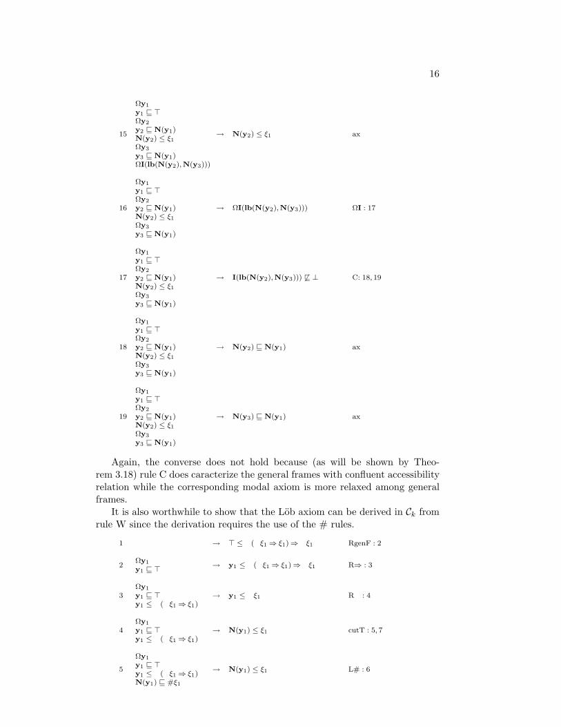
→ I(lb(N(y2),N(y3))) 6v ⊥ C: 18, 19
18
Ωy1
y1 v >Ωy2
y2 v N(y1)N(y2) ≤ ξ1Ωy3
y3 v N(y1)
→ N(y2) v N(y1) ax
19
Ωy1
y1 v >Ωy2
y2 v N(y1)N(y2) ≤ ξ1Ωy3
y3 v N(y1)
→ N(y3) v N(y1) ax
Again, the converse does not hold because (as will be shown by Theo-rem 3.18) rule C does caracterize the general frames with confluent accessibilityrelation while the corresponding modal axiom is more relaxed among generalframes.
It is also worthwhile to show that the Lob axiom can be derived in Ck fromrule W since the derivation requires the use of the # rules.
1 → > ≤ (ξ1 ⇒ ξ1)⇒ξ1 RgenF : 2
2Ωy1
y1 v > → y1 ≤ (ξ1 ⇒ ξ1)⇒ξ1 R⇒ : 3
3Ωy1
y1 v >y1 ≤ (ξ1 ⇒ ξ1)
→ y1 ≤ ξ1 R : 4
4Ωy1
y1 v >y1 ≤ (ξ1 ⇒ ξ1)
→ N(y1) ≤ ξ1 cutT : 5, 7
5
Ωy1
y1 v >y1 ≤ (ξ1 ⇒ ξ1)N(y1) v #ξ1
→ N(y1) ≤ ξ1 L# : 6

17
6
Ωy1
y1 v >y1 ≤ (ξ1 ⇒ ξ1)N(y1) ≤ ξ1
→ N(y1) ≤ ξ1 ax
7Ωy1
y1 v >y1 ≤ (ξ1 ⇒ ξ1)
→ N(y1) ≤ ξ1N(y1) v #ξ1
W: 8
8
Ωy1
y1 v >y1 ≤ (ξ1 ⇒ ξ1)Ωy2
y2 v N(y1)
→N(y1) ≤ ξ1y2 v #ξ1N(y2) 6v #ξ1
R# : 9
9
Ωy1
y1 v >y1 ≤ (ξ1 ⇒ ξ1)Ωy2
y2 v N(y1)
→N(y1) ≤ ξ1y2 ≤ ξ1N(y2) 6v #ξ1
RxiT : 10
10
Ωy1
y1 v >y1 ≤ (ξ1 ⇒ ξ1)Ωy2
y2 v N(y1)N(y2) v #ξ1
→ N(y1) ≤ ξ1y2 ≤ ξ1
L# : 11
11
Ωy1
y1 v >y1 ≤ (ξ1 ⇒ ξ1)Ωy2
y2 v N(y1)N(y2) ≤ ξ1
→ N(y1) ≤ ξ1y2 ≤ ξ1
LxeT : 12
12
Ωy1
y1 v >y1 ≤ (ξ1 ⇒ ξ1)Ωy2
y2 v N(y1)
→N(y1) ≤ ξ1y2 ≤ ξ1N(y2) 6≤ ξ1
L : 13
13
Ωy1
y1 v >N(y1) ≤ ξ1 ⇒ ξ1Ωy2
y2 v N(y1)
→N(y1) ≤ ξ1y2 ≤ ξ1N(y2) 6≤ ξ1
LgenT : 14, 15, 16
14
Ωy1
y1 v >Ωy2
y2 v N(y1)
→N(y1) ≤ ξ1y2 ≤ ξ1N(y2) 6≤ ξ1Ωy2
ax
15
Ωy1
y1 v >Ωy2
y2 v N(y1)
→N(y1) ≤ ξ1y2 ≤ ξ1N(y2) 6≤ ξ1y2 v N(y1)
ax
16
Ωy1
y1 v >y2 ≤ ξ1 ⇒ ξ1Ωy2
y2 v N(y1)
→N(y1) ≤ ξ1y2 ≤ ξ1N(y2) 6≤ ξ1
L⇒ : 17, 18

18
17
Ωy1
y1 v >y2 ≤ ξ1Ωy2
y2 v N(y1)
→N(y1) ≤ ξ1y2 ≤ ξ1N(y2) 6≤ ξ1
ax
18
Ωy1
y1 v >Ωy2
y2 v N(y1)
→N(y1) ≤ ξ1y2 ≤ ξ1N(y2) 6≤ ξ1y2 ≤ ξ1
R : 19
19
Ωy1
y1 v >Ωy2
y2 v N(y1)
→N(y1) ≤ ξ1y2 ≤ ξ1N(y2) 6≤ ξ1N(y2) ≤ ξ1
RxiF : 20
20
Ωy1
y1 v >Ωy2
y2 v N(y1)N(y2) ≤ ξ1
→N(y1) ≤ ξ1y2 ≤ ξ1N(y2) ≤ ξ1
ax
Obviously, the converse does not hold since (as will be shown by Theo-rem 3.18) rule W does caracterize the general frames with transitive and wellbounded accessibility relation while Lob’s axiom is more relaxed among generalframes.
This provides the basis for giving other rules for modal and other non-classical logics. A detailed discussion of such rules and of the semantic andproof-theoretic properties of the resulting labelled sequent calculi (e.g. a formof correspondence theory [18] or the eliminability of cut) is out of the scope ofthis paper and we leave it as future work.
2.7 Towards a hybrid version of CK
The discussion above (about, for instance, the non inter-derivability of ruleT and the modal axiom for reflexivity) motivates the following question: is itpossible to enrich CK in order to recover that inter-derivability? Semantically, aswe saw, this will mean moving from general Kripke semantics towards standardKripke semantics (as we shall further comment at the end of Subsection 3.3).
The answer turns out to be surprisingly simple and possibly useful for otherpurposes. It is enough: (i) first, to enrich the language with a coercion operator@ transforming any term t into a simple formula @t; (ii) and, second, add thefollowing order rules:
L@ τ1vτ2,Γ1→Γ2
τ1≤@τ2,Γ1→Γ2R@ Γ1→Γ2,τ1vτ2
Γ1→Γ2,τ1≤@τ2
In this way we established an enrichment of CK that we denote by C@K . In this
enriched calculus, it is possible to derive, for instance, rule T from the modalaxiom for reflexivity:
1 Ωτ1 → τ1 v N(τ1) cutF : 2, 6
2 Ωτ1 → τ1 v N(τ1)τ1 ≤ @N(τ1)⇒@N(τ1)
transF : 3, 4

19
3 Ωτ1 → τ1 v N(τ1)τ1 v > >
4 Ωτ1 → τ1 v N(τ1)> ≤ @N(τ1)⇒@N(τ1)
w : 5
5 → > ≤ @N(τ1)⇒@N(τ1) hyp
6Ωτ1τ1 ≤ @N(τ1)⇒@N(τ1)
→ τ1 v N(τ1) L⇒ : 7, 9
7Ωτ1τ1 ≤ @N(τ1)
→ τ1 v N(τ1) L@ : 8
8Ωτ1τ1 v N(τ1)
→ τ1 v N(τ1) ax
9 Ωτ1 → τ1 v N(τ1)τ1 ≤ @N(τ1)
R : 10
10 Ωτ1 → τ1 v N(τ1)N(τ1) ≤ @N(τ1)
R@ : 11
11 Ωτ1 → τ1 v N(τ1)N(τ1) v N(τ1)
ref
The same holds for the other properties of the accessibility relation but werefrain from going into details.
The sequent calculus C@K represents a first step towards a hybrid version of
CK combining the ideas in this paper and those of hybrid logics [7, 6, 2].
2.8 Local and global reasoning
In the context of a modal sequent calculus, local and global notions of proof-theoretic consequence can be defined as follows:
• ψ1, . . . , ψk `gR ϕ iff `R > ≤ ψ1, . . . ,> ≤ ψk → > ≤ ϕ;
• ψ1, . . . , ψk ``R ϕ iff `R Ωy1,y1 ≤ ψ1, . . . ,y1 ≤ ψk → y1 ≤ ϕ.
Thus, ϕ is globally derived from ψ1, . . . , ψk provided that ϕ is true (>)whenever ψi is true for all i = 1, . . . k. When working with worlds this meansthat the denotation ϕ is W whenever the denotation of ψi is W for all i = 1, . . . k.
On the other hand, ϕ is locally derived from ψ1, . . . , ψk provided that forevery atomic element y1 the value of ϕ is greater than or equal to the value ofy1 whenever the value of ψi is greater than or equal to the value of y1 for alli = 1, . . . k. When working with worlds we get the usual definition stating thatϕ is true at w whenever ψi is true at w for all i = 1, . . . k.
Lemma 2.3 Within the context of a modal sequent calculus:
1. Ωy1,y1 ≤ ψ1, . . . ,y1 ≤ ψk → y1 ≤ ϕ `R → > ≤ ((ψ1 ∧ . . . ∧ ψk)⇒ ϕ);
2. → > ≤ ((ψ1 ∧ . . . ∧ ψk)⇒ ϕ) `R Ωy1,y1 ≤ ψ1, . . . ,y1 ≤ ψk → y1 ≤ ϕ.
Proof: Without loss of generality consider k = 2.1. Consider the following derivation:

20
1 → > ≤ ((ψ1 ∧ ψ2)⇒ ϕ) RgenF : 2
2Ωy1
y1 v > → y1 ≤ ((ψ1 ∧ ψ2)⇒ ϕ) R⇒ : 3
3Ωy1
y1 v >y1 ≤ (ψ1 ∧ ψ2)
→ y1 ≤ ϕ L∧ : 4
4
Ωy1
y1 v >y1 ≤ ψ1
y1 ≤ ψ2
→ y1 ≤ ϕ Lw : 5
5Ωy1
y1 ≤ ψ1
y1 ≤ ψ2
→ y1 ≤ ϕ hyp
2. Consider the following derivation:
1Ωy1
y1 ≤ ψ1
y1 ≤ ψ2
→ y1 ≤ ϕ cutF : 2, 3
2Ωy1
y1 ≤ ψ1
y1 ≤ ψ2
→ y1 ≤ ϕy1 ≤ ((ψ1 ∧ ψ2)⇒ ϕ)
transF : 4, 9
3
Ωy1
y1 ≤ ψ1
y1 ≤ ψ2
y1 ≤ ((ψ1 ∧ ψ2)⇒ ϕ)
→ y1 ≤ ϕ L⇒ : 5, 6
4Ωy1
y1 ≤ ψ1
y1 ≤ ψ2
→ y1 ≤ ϕy1 v > >
5Ωy1
y1 ≤ ψ1
y1 ≤ ψ2
→ y1 ≤ ϕy1 ≤ (ψ1 ∧ ψ2)
R∧ : 7, 8
6
Ωy1
y1 ≤ ψ1
y1 ≤ ψ2
y1 ≤ ϕ
→ y1 ≤ ϕ ax
7Ωy1
y1 ≤ ψ1
y1 ≤ ψ2
→ y1 ≤ ϕy1 ≤ ψ1
ax
8Ωy1
y1 ≤ ψ1
y1 ≤ ψ2
→ y1 ≤ ϕy1 ≤ ψ2
ax
9Ωy1
y1 ≤ ψ1
y1 ≤ ψ2
→ y1 ≤ ϕ> ≤ ((ψ1 ∧ ψ2)⇒ ϕ)
ws : 10
10 → > ≤ ((ψ1 ∧ ψ2)⇒ ϕ) hyp
QED
With this lemma it is straightforward to establish the following result relat-ing global and local reasoning.
Proposition 2.4 Within any modal sequent calculus: ψ1, . . . , ψk ``R ϕ iff
`gR (ψ1 ∧ . . . ∧ ψk)⇒ ϕ.

21
Proof: Indeed, ψ1, . . . , ψk ``R ϕ iff `R Ωy1,y1 ≤ ψ1, . . . ,y1 ≤ ψk → y1 ≤ ϕ
iff (using Lemma 2.3 and taking into account idempotence in Proposition 2.1)`R → > ≤ ((ψ1 ∧ . . . ∧ ψk)⇒ ϕ) iff `g
R (ψ1 ∧ . . . ∧ ψk)⇒ ϕ. QED
2.9 Metatheorems
It is useful to denote by ∆ the bag δ : δ ∈ ∆. Then, it is straightforward toprove the following result taking into account that the conjugate of a conjugateof an assertion is the original assertion:
Theorem 2.5 (Metatheorem of conjugation) Let C be a structural sequentcalculus. Then, for every set S of ground sequents and every ground sequent∆′ → ∆′′:
S `C ∆′ → ∆′′ iff S `C → ∆′′, ∆′ .
The two following metatheorems will also be useful later on when establish-ing the completeness theorem.
Theorem 2.6 (Metatheorem of contradiction) Let C be a structural se-quent calculus. Then, for every set S of ground sequents and every groundsequent → ∆, if
S `C → ∆ (∗)S `C → δ for every δ ∈ ∆ (∗∗)
then S `C → υ for every ground assertion υ.
Proof: Let ∆ be δ1, δ2 without loss of generality. Then:
1 → υ cut : 2, 52 δ1 → υ Rx : 3
3 → υ, δ1 Rw : 4
4 → δ1 (**)5 → υ, δ1 cut : 6, 96 δ2 → υ, δ1 Rx : 7
7 → υ, δ1, δ2 Rws : 8
8 → δ2 (**)9 → υ, δ1, δ2 Rw : 1010 → δ1, δ2 (*)
QED
Theorem 2.7 (Metatheorem of deduction) Let C be a structural sequentcalculus with rules endowed with persistent provisos. Then, for every set S ofground sequents and closed sequent δ′1, . . . , δ
′m → ∆′′:
S `C δ′1, . . . , δ′m → ∆′′ iff S, → δ′1, . . . , → δ′m `C → ∆′′ .
Proof:(⇒) Assume S `C δ′1, . . . , δ
′m → ∆′′ with derivation sequence D. Then, the
following sequence outline establishes S, → δ′1, . . . , → δ′m `C → ∆′′:

22
1 → ∆′′ cut : 2, 32 → ∆′′, δ′1 Rws : 43 δ′1 → ∆′′ cut : 5, 64 → δ′1 hyp5 δ′1 → ∆′′, δ′2 Rws : 76 δ′2, δ′1 → ∆′′ cut : 9, 107 δ′1 → δ′2 Lw : 88 → δ′2 hyp
. . .i δ′1, . . . , δ′m → ∆′′ D
(⇐) Assume S, → δ′1, . . . , → δ′m `C → ∆′′ with the derivation sequenced1, . . . , dn. Then we can build a derivation of S `C δ′1, . . . , δ
′m → ∆′′ by changing
each di = Θi1 → Θi
2 to d′i = δ′1, . . . , δ′m,Θi
1 → Θi2 replacing the justification hyp
on each di =→ δ′j by ax. Observe that the sequence d′1, . . . , d′n does constitute
a derivation because the unchanged justifications still hold thanks to the factthat δ′1, . . . , δ
′m are closed assertions and therefore any (persistent) proviso that
otherwise might be violated is still fulfilled. QED
Therefore, the metatheorem of deduction holds in any modal sequent calcu-lus as defined at the end of Subsection 2.5 (precluding the use of non persistentprovisos).
3 Semantics
3.1 Algebraic semantics
Let Σ = 〈C, O,X, Y, Z〉 be a signature. A Σ-algebra is a triple A = 〈F, T, ·A〉where:
• F and T are sets;
• ·A is a map such that:
– cA : F k → F for each c ∈ Ck;
– oA : T k → T for each o ∈ Ok;
– #A : F → T ;
– ΩA ⊆ T ;
– vA ⊆ T × T ;
– ≤A ⊆ T × F .
Let A be a Σ-algebra. An unbound variable assignment over A is a map αthat maps each element of X to an element of T and each element of Z to anelement of F . A bound variable assignment over A is a map β from Y to T .
The denotation at Σ-algebra A for unbound variable assignment α of groundsimple formulae is inductively defined with the following rules:
• [[z]]Aα = α(z);
• [[c(ϕ1, . . . , ϕk)]]Aα = cA([[ϕ1]]Aα, . . . , [[ϕk]]Aα).

23
The denotation at A for assignments α, β over A of ground terms is induc-tively defined with the following rules:
• [[x]]Aαβ = α(x);
• [[y]]Aαβ = β(y);
• [[o(θ1, . . . , θk)]]Aαβ = oA([[θ1]]Aαβ , . . . , [[θk]]Aαβ);
• [[#ϕ]]Aαβ = #A([[ϕ]]Aα).
The satisfaction by A for α, β of ground assertions and sequents is definedas follows:
• Aαβ ° Ωθ iff [[θ]]Aαβ ∈ ΩA;
• Aαβ ° fθ iff [[θ]]Aαβ /∈ ΩA;
• Aαβ ° θ v θ′ iff 〈[[θ]]Aαβ , [[θ′]]Aαβ〉 ∈ vA;
• Aαβ ° θ 6v θ′ iff 〈[[θ]]Aαβ , [[θ′]]Aαβ〉 /∈ vA;
• Aαβ ° θ ≤ ϕ iff 〈[[θ]]Aαβ , [[ϕ]]Aα〉 ∈ ≤A;
• Aαβ ° θ 6≤ ϕ iff 〈[[θ]]Aαβ , [[ϕ]]Aα〉 /∈ ≤A;
• Aαβ ° ∆′ → ∆′′ iff Aαβ ° δ for some δ ∈ ∆′′ ∪∆′.
Furthermore, the satisfaction by A for α of ground assertions and sequentsis defined as follows:
• Aα ° δ iff Aαβ ° δ for every bound variable assignment β over A;
• Aα ° ∆′ → ∆′′ iff Aαβ ° ∆′ → ∆′′ for every bound variable assignmentβ over A.
Observe that, when dealing with closed simple formulae, terms, assertionsand sequents, we may drop the reference to the assignments in denotationsand satisfactions since they do not depend on them. For instance, if δ is aclosed assertion then we may write A ° δ since, for any assignments α, α′, β, β′,Aαβ ° δ iff Aα′β′ ° δ. A similar principle applies when we deal with terms,assertions and sequents without bound variables in which case we may dropthe reference to the bound variable assignment. In the same vein, we may dropthe reference to the unbound variable assignment when dealing with terms,assertions and sequents without unbound variables.
Given a class A of Σ-algebras, a ground sequent s is A-entailed by theground sequents s1, . . . , sp, written s1, . . . , sp ²A s, iff, for each A ∈ A andunbound variable assignment α over A, Aα ° s whenever Aα ° si for everyi = 1, . . . , p.
The notion of entailment is easily extended to (schema) sequents possiblywith provisos. A sequent s is A-entailed by the sequents s1, . . . , sp with pro-viso π, written s1, . . . , sp ²A s C π, iff s1ρ, . . . , spρ ²A sρ for every groundsubstitution ρ over Σ such that π(ρ) = 1.
The following results are the semantic counterparts of Proposition 2.1 andProposition 2.2.

24
Proposition 3.1 Given a class A of Σ-algebras:
Projective If S ²A s′ C π and π′ ⊆ π then S ²A s′ C π′.
Extensive S ²A s C up for each sequent s ∈ S.
Monotonic If S ⊆ S1 and S ²A s′ C π then S1 ²A s′ C π.
Idempotent If S1 ²A s C πs for each s in a finite set S of sequents andS ²A s′ C π then S1 ²A s′ C π ∩ (
⋂
s∈S
πs).
Proof: Straightforward. We prove only the last property. Assume S1 ²A s C πs
for each sequent s ∈ S and S ²A s′ C π. So, by the projective property,S1 ²A s C π ∩ (
⋂s∈S πs) for each sequent s ∈ S and S ²A s′ C π ∩ (
⋂s∈S πs).
Thus, by definition of entailment, for every ρ such that (π ∩ (⋂
s∈S πs))(ρ) = 1,S1ρ ²A sρ for each sequent s ∈ S and Sρ ²A s′ρ. Therefore, for every such ρ,every A ∈ A and unbound variable assignment α over A: (i) if Aα ° s1ρ forevery s1 ∈ S1 then Aα ° sρ for every s ∈ S; and (ii) if Aα ° sρ for every s ∈ Sthen Aα ° s′ρ. So, for every such ρ, every A ∈ A and α, if Aα ° s1ρ for everys1 ∈ S1 then Aα ° s′ρ. QED
Proposition 3.2 Given a class A of Σ-algebras, for every substitution σ, ifS ²A s′ C π then Sσ ²A s′σ C πσ.
Proof: We have to show Sσ ²A s′σ C πσ. That is, for an arbitrary groundsubstitution ρ such that (πσ)(ρ) = 1, we have to show (Sσ)ρ ²A (s′σ)ρ. Byhypothesis, we know S ²A s′ C π. That is, for every ground substitutionρ′ such that π(ρ′) = 1, we know Sρ′ ²A s′ρ′. Since the substitution σρ isground and, furthermore, π(σρ) = (πσ)(ρ) = 1, we know from the hypothesisS(σρ) ²A s′(σρ) which establishes the thesis taking into account the followingproperty of substitutions δ(σρ) = (δσ)ρ. QED
A classA of Σ-algebras is said to be appropriate for a Σ-rule 〈s1, . . . , sp, s, π〉if s1, . . . , sp ²A s C π. And an algebra A is said to be appropriate for a rule ifso is the class A.
Theorem 3.3 (Structural soundness) The class of all Σ-algebras is appro-priate for every structural rule over Σ.
Proof: It is straighforward to verify the thesis for each of the structural rules.For instance, consider the rule RwT. We have to verify that, for each Σ-algebraA, assignment α and ground substitution ρ, if Aα ° Γ1ρ → Γ2ρ then Aα °Γ1ρ → Γ2ρ, τ1ρ v τ2ρ. Assume that Aα ° Γ1ρ → Γ2ρ. That is, for everyassignment β, Aαβ ° Γ1ρ → Γ2ρ. Thus, for every assignment β there isδ ∈ Γ2ρ ∪ Γ1ρ such that Aαβ ° δ. So, for every assignment β there is δ ∈Γ2ρ∪τ1ρ v τ2ρ∪Γ1ρ such that Aαβ ° δ. Therefore, for every assignment β,Aαβ ° Γ1ρ → Γ2ρ, τ1ρ v τ2ρ. That is, Aα ° Γ1ρ → Γ2ρ, τ1ρ v τ2ρ. QED
25
A class A of Σ-algebras is said to be appropriate for a sequent calculus〈Σ,R〉 if it is appropriate for each proper rule in R (and also for the structuralrules thanks to the theorem above). And an algebra A is said to be appropriatefor a sequent calculus if so is the class A.
A (sequent) logic is a triple L = 〈Σ,R,A〉 where 〈Σ,R〉 is a sequent calculusand A is a class of Σ-algebras. A sequent logic is said to be:
• sound if A is appropriate for 〈Σ,R〉;• full if A is the class of all Σ-algebras that are appropriate for 〈Σ,R〉;• complete if s1, . . . , sp `R s whenever s1, . . . , sp ²A s for any closed se-
quents s, s1, . . . , sp.
Thus, every full logic is sound. Furthermore:
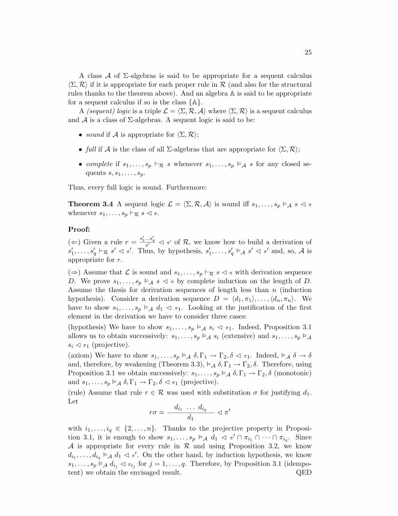
Theorem 3.4 A sequent logic L = 〈Σ,R,A〉 is sound iff s1, . . . , sp ²A s C π
whenever s1, . . . , sp `R s C π.
Proof:
(⇐) Given a rule r = s′1...s′qs′ C π′ of R, we know how to build a derivation of
s′1, . . . , s′q `R s′ C π′. Thus, by hypothesis, s′1, . . . , s
′q ²A s′ C π′ and, so, A is
appropriate for r.
(⇒) Assume that L is sound and s1, . . . , sp `R s C π with derivation sequenceD. We prove s1, . . . , sp ²A s C π by complete induction on the length of D.Assume the thesis for derivation sequences of length less than n (inductionhypothesis). Consider a derivation sequence D = 〈d1, π1〉, . . . , 〈dn, πn〉. Wehave to show s1, . . . , sp ²A d1 C π1. Looking at the justification of the firstelement in the derivation we have to consider three cases:(hypothesis) We have to show s1, . . . , sp ²A si C π1. Indeed, Proposition 3.1allows us to obtain successively: s1, . . . , sp ²A si (extensive) and s1, . . . , sp ²Asi C π1 (projective).(axiom) We have to show s1, . . . , sp ²A δ, Γ1 → Γ2, δ C π1. Indeed, ²A δ → δand, therefore, by weakening (Theorem 3.3), ²A δ,Γ1 → Γ2, δ. Therefore, usingProposition 3.1 we obtain successively: s1, . . . , sp ²A δ,Γ1 → Γ2, δ (monotonic)and s1, . . . , sp ²A δ,Γ1 → Γ2, δ C π1 (projective).(rule) Assume that rule r ∈ R was used with substitution σ for justifying d1.Let
rσ =di1 . . . diq
d1C π′
with i1, . . . , iq ∈ 2, . . . , n. Thanks to the projective property in Proposi-tion 3.1, it is enough to show s1, . . . , sp ²A d1 C π′ ∩ πi1 ∩ · · · ∩ πiq . SinceA is appropriate for every rule in R and using Proposition 3.2, we knowdi1 , . . . , diq ²A d1 C π′. On the other hand, by induction hypothesis, we knows1, . . . , sp ²A dij C πij for j = 1, . . . , q. Therefore, by Proposition 3.1 (idempo-tent) we obtain the envisaged result. QED

26
A sequent logic L = 〈Σ,R,A〉 is said to be structural/order/modal if itscalculus 〈Σ,R〉 is structural/order/modal, respectively.
Within a modal logic, besides the local and global notions of proof-theoreticconsequence presented before, we can also introduce their model-theoretic coun-terparts:
• ψ1, . . . , ψk ²gA ϕ iff ²A > ≤ ψ1, . . . ,> ≤ ψk → > ≤ ϕ;
• ψ1, . . . , ψk ²`A ϕ iff ²A Ωy1,y1 ≤ ψ1, . . . ,y1 ≤ ψk → y1 ≤ ϕ.
The following result is the semantic counterpart of Proposition 2.4.
Proposition 3.5 Within the context of a sound modal sequent logic L =〈Σ,R,A〉: ψ1, . . . , ψk ²`
A ϕ iff ²gA (ψ1 ∧ . . . ∧ ψk)⇒ ϕ.
Proof: Taking into account Theorem 3.4, from Lemma 2.3 we obtain:
1. Ωy1,y1 ≤ ψ1, . . . ,y1 ≤ ψk → y1 ≤ ϕ ²A → > ≤ ((ψ1 ∧ . . . ∧ ψk)⇒ ϕ);
2. → > ≤ ((ψ1 ∧ . . . ∧ ψk)⇒ ϕ) ²A Ωy1,y1 ≤ ψ1, . . . ,y1 ≤ ψk → y1 ≤ ϕ.
Therefore, ψ1, . . . , ψk ²`A ϕ iff ²A Ωy1,y1 ≤ ψ1, . . . ,y1 ≤ ψk → y1 ≤ ϕ iff
(from 1. and 2. taking into account idempotence in Proposition 3.1) ²A → > ≤((ψ1 ∧ . . . ∧ ψk)⇒ ϕ) iff ²g
A (ψ1 ∧ . . . ∧ ψk)⇒ ϕ. QED
3.2 Algebraic completeness
A set S of closed sequents is said to be consistent if for no closed assertion δboth → δ ∈ S and → δ ∈ S hold. And it is said to be maximal consistent if forevery closed assertion δ either → δ ∈ S or → δ ∈ S but not both.
Given a sequent calculus C = 〈Σ,R〉 and a maximal consistent set S ofclosed sequents over Σ, the syntactic algebra induced by C and S is the followingΣ-algebra:
A(C, S) = 〈cgF(Σ), cgT(Σ), ·A(C,S)〉where:
• cA(C,S) = λf1 . . . fk. c(f1, . . . , fk);
• oA(C,S) = λt1 . . . tk. o(t1, . . . , tk);
• #A(C,S) = λf. #f ;
• θ ∈ ΩA(C,S) iff S `C → Ωθ;
• 〈θ, θ′〉 ∈ vA(C,S) iff S `C → θ v θ′;
• 〈θ, ϕ〉 ∈ ≤A(C,S) iff S `C → θ ≤ ϕ.

27
Let ϕ ∈ gF(Σ). Given an unbounded variable assignment α over a syntacticalgebra A(C, S), we denote by ϕα the closed simple formula obtained from ϕby replacing each variable z ∈ Z by α(z).
Let θ ∈ gT(Σ). Given an unbounded variable assignment α and a boundedvariable assignment β both over a syntactic algebra A(C, S), we denote by θαβthe closed term obtained from θ by replacing each variable x ∈ X by α(x) andeach variable y ∈ Y by β(y).
This notation is extended to ground assertions and bags of ground assertionsby identifying ϕαβ with ϕα.
Lemma 3.6 Let C be a structural calculus, S a maximal consistent set ofclosed sequents, α an unbound variable assignment over A(C, S), β a boundvariable assignment over A(C, S), ϕ a ground simple formula, and θ a groundterm. Then:
• [[ϕ]]A(C,S)α = ϕα;
• [[θ]]A(C,S)αβ = θαβ.
Proof: Straightforward induction on the complexity of simple formula ϕ andterm θ, respectively. QED
Lemma 3.7 Let C be a structural calculus, S a maximal consistent set of closedsequents, α an unbound variable assignment over A(C, S), β a bound variableassignment over A(C, S), and δ a ground assertion. Then:
A(C, S)αβ ° δ iff S `C → δαβ .
Proof:
(i) A(C, S)αβ ° Ωθ iff [[θ]]A(C,S)αβ ∈ ΩA(C,S) iff (by Lemma 3.6) θαβ ∈ ΩA(C,S)
iff S `C → Ω(θαβ) iff S `C → (Ωθ)αβ.
(ii) Both A(C, S)αβ ° θ v θ′ iff S `C → (θ v θ′)αβ and A(C, S)αβ ° θ ≤ ϕ iffS `C → (θ ≤ ϕ)αβ are obtained in a similar way.
(iii) A(C, S)αβ ° fθ iff [[θ]]A(C,S)αβ 6∈ ΩA(C,S) iff (by Lemma 3.6) θαβ 6∈ ΩA(C,S)
iff S 6`C → Ω(θαβ) iff (since S is maximal consistent) S `C → f(θαβ) iffS `C → (fθ)αβ.
(iv) Again, both A(C, S)αβ ° θ 6v θ′ iff S `C → (θ 6v θ′)αβ and A(C, S)αβ °θ 6≤ ϕ iff S `C → (θ 6≤ ϕ)αβ are obtained in a similar way. QED
Lemma 3.8 (Lifting) Let C be a structural calculus, S a maximal consistentset of closed sequents, α an unbound variable assignment over A(C, S), β abound variable assignment over A(C, S), and ∆′ → ∆′′ a ground sequent. Then:
A(C, S)αβ ° ∆′ → ∆′′ iff S `C ∆′αβ → ∆′′αβ .

28
Proof: Indeed, A(C, S)αβ ° ∆′ → ∆′′ iff A(C, S)αβ ° δ for some δ ∈ ∆′′ ∪∆′iff (Lemma 3.7) S `C → δαβ for some δ ∈ ∆′′ ∪∆′ iff S `C → δ for some δ ∈∆′′αβ∪∆′αβ iff (see justification below) S `C → ∆′′αβ, ∆′αβ iff (Theorem 2.5),S `C ∆′αβ → ∆′′αβ. It remains to explain:(1) If S `C → δ for some δ ∈ ∆′′αβ ∪ ∆′αβ then S `C → ∆′′αβ, ∆′αβ. Thisfact is trivially obtained by applications of right weakening.(2) If S `C → ∆′′αβ, ∆′αβ then S `C → δ for some δ ∈ ∆′′αβ ∪∆′αβ. Indeed,otherwise, since S is maximal consistent, S `C → δ for every δ ∈ ∆′′αβ∪∆′αβ.Then, using Theorem 2.6, we would be able to show that every closed assertionis derivable from S, therefore contradicting that S is consistent. QED
Observe that, in the conditions of the previous lemma, if, furthermore, thesequent ∆′ → ∆′′ is closed then we have:
A(C, S) ° ∆′ → ∆′′ iff S `C ∆′ → ∆′′ .
Lemma 3.9 (Appropriateness) The class of all syntactic algebras inducedby a sequent calculus is appropriate for it.
Proof: Let r = s1...sp
s be a ground instance of a (proper) rule of a sequentcalculus C. Let α be an arbitrary unbound variable assignment over a syntacticalgebra A(C, S). Assume that A(C, S)α ° si for each i = 1, . . . , p. That is, forevery bound variable assignment β, A(C, S)αβ ° si for each i = 1, . . . , p. So, byLemma 3.8, for every such β, S `C siαβ, say with derivation sequence Dsiαβ, foreach such i. Then, it is straightforward to build, for every pair α, β, a derivationsequence for S `C sαβ using rule r and those derivation sequences. Thus, againby Lemma 3.8, for every such β, A(C, S)αβ ° s. That is, A(C, S)α ° s. QED
Lemma 3.10 (Consistent extension) Let C be a structural sequent calculuswith rules endowed with persistent provisos. If S is a consistent set of closedsequents and S 6`C→ υ1, . . . , υm for closed assertions υ1, . . . , υm then the setS ∪ →υ1, . . . ,→υm is still consistent.
Proof: Assume that S ∪ →υ1, . . . ,→υm is inconsistent. Then, there is aclosed assertion δ such that S,→υ1, . . . ,→υm `C → δ and S,→υ1, . . . ,→υm `C→ δ. So, using the metatheorem of contradiction (Theorem 2.6),
S,→υ1, . . . ,→υm `C → υ1 .
Therefore, using the metatheorem of deduction (Theorem 2.7),
S `C υ1, . . . , υm → υ1 .
Thus, applying the metatheorem of conjugation (Theorem 2.5), we get
S `C → υ1, υ1, υ2, . . . , υm
and, by right contraction,
S `C → υ1, . . . , υm
which contradicts the second hypothesis. QED

29
Theorem 3.11 (Algebraic completeness) Every full structural sequent logicwith rules endowed with persistent provisos is complete.
Proof: Consider the logic L = 〈Σ,R,A〉 and let C = 〈Σ,R〉. Assume thatS 6`R ∆′ → ∆′′ with S ∪ ∆′ → ∆′′ composed of closed sequents.Given an enumeration υn with n ∈ N of the set of closed assertions, we startby extending S to a maximal consistent set S• as follows:
• S0 = S ∪ →δ : δ ∈ ∆′′ ∪∆′;
• Sn+1 =
S ∪ →υn provided that Sn `R → υn
S ∪ →υn otherwise;
• S• =⋃
n∈NSn.
Observe that S• is still consistent thanks to Lemma 3.10. Furthermore, byconstruction, it is maximal consistent. Therefore, S• 6`R ∆′ → ∆′′ becauseotherwise S• `R → δ for some δ ∈ ∆′′ ∪∆′ (using the same reasoning as in jus-tification (2) in the proof of Lemma 3.8) and, hence, S• would be inconsistent.Thus, by Lemma 3.8 applied to a closed sequent, A(C, S•) 6° ∆′ → ∆′′.On the other hand, for every s ∈ S we know that S `R s and, thus, againthanks to Lemma 3.8, A(C, S•) ° s.Since the logic is full and taking into account Lemma 3.9, A(C, S•) is in A.Hence, S 6²A ∆′ → ∆′′. QED
Corollary 3.12 (Modal algebraic completeness) Within the context of afull modal sequent logic L = 〈ΣK ,R,A〉:
1. ψ1, . . . , ψk `gR ϕ iff ψ1, . . . , ψk ²g
A ϕ;
2. ψ1, . . . , ψk ``R ϕ iff ψ1, . . . , ψk ²`
A ϕ.
Proof:1. ψ1, . . . , ψk `g
R ϕ iff (by definition) `R > ≤ ψ1, . . . ,> ≤ ψk → > ≤ ϕ iff (⇒:since L is full and therefore sound; ⇐: thanks to the completeness theoremabove, since we are dealing with closed sequents and modal logics are assumedto use only persistent provisos) ²A > ≤ ψ1, . . . ,> ≤ ψk → > ≤ ϕ iff (bydefinition) ψ1, . . . , ψk ²g
A ϕ.
2. ψ1, . . . , ψk ``R ϕ iff (by Proposition 2.4) `g
R (ψ1 ∧ . . . ∧ ψk)⇒ ϕ iff (by 1.)²gA (ψ1 ∧ . . . ∧ ψk)⇒ ϕ iff (by Proposition 3.5) ψ1, . . . , ψk ²`
A ϕ. QED
3.3 Kripke completeness
We now turn our attention to the traditional semantics of modal logic (basedon, possibly general, Kripke structures). Namely, it is worthwhile to analyze theclass of Kripke structures characterized by a given set of rules. More precisely,we would like to prove that, for instance, rule T does characterize the reflexiveframes. It would also be nice to establish soundness and completeness results

30
over general Kripke semantics by capitalizing on the algebraic completenesstheorem proved in the previous subsection.
Given a suitable choice function needed for interpreting I, it is straight-forward to extract from any (possibly general) Kripke structure a ΣK-algebrawhile respecting the denotation of ground simple formulae. Recall that ΣK =〈C,O, X, Y, Z〉 is the modal signature introduced in Subsection 2.5.
Let K = 〈W,Ã,B, V 〉 be a general Kripke structure over C where W isthe non-empty set of worlds, Ã is the accessibility relation between worlds,B ⊆ ℘W is the set of admissible truth values, and the valuation V maps eachpropositional symbol pi to an admissible truth value. Let ι be a choice functionfor W . Then, the ΣK-algebra Alg(K) = 〈F, T, ·Alg(K)〉 induced byK is as follows:
• F = B;
• T = ℘W ;
• #Alg(K) = λb. b;
• a ∈ ΩAlg(K) iff a is a singleton;
• 〈a, a′〉 ∈ vAlg(K) iff a ⊆ a′;
• 〈a, b〉 ∈ ≤Alg(K) iff a ⊆ b;
• ⊥Alg(K) = ∅;• >Alg(K) = W ;
• IAlg(K) = λa. ι(a);
• NAlg(K) = λa. w′ ∈ W : exists w ∈ a such that w à w′;• lbAlg(K) = λaa′. a ∩ a′;
• fAlg(K) = ∅;• tAlg(K) = W ;
• piAlg(K) = V (pi);
• ¬Alg(K) = λb. W \ b;
• ¤Alg(K) = λb. w ∈ W : NAlg(K)(w) ⊆ b;• ♦Alg(K) = λb. w ∈ W : NAlg(K)(w) ∩ b 6= ∅;• ∧Alg(K) = λbb′. b ∩ b′;
• ∨Alg(K) = λbb′. b ∪ b′;
• ⇒Alg(K) = λbb′. (W \ b) ∪ b′.
It is straightforward to verify the following facts that will allow us later onto concentrate on the semantics of f ,pi,¬,¤,∨.

31
• tAlg(K) = ¬Alg(K)(fAlg(K));
• ♦Alg(K)(b) = ¬Alg(K)(¤Alg(K)(¬Alg(K)(b)));
• ⇒Alg(K)(b, b′) = ∨Alg(K)(¬Alg(K)(b), b′);
• ∧Alg(K)(b, b′) = ¬Alg(K)(∨Alg(K)(¬Alg(K)(b),¬Alg(K)(b′))).
The following results show that the semantics of closed simple formulae ispreserved when we move from a general Kripke structure to the correspondingΣK-algebra. In the sequel we use [[ϕ]]K for the denotation of ϕ over the generalKripke structure K. This denotation is inductively defined over the structureof ϕ in the usual way.
Lemma 3.13 Let K be a general Kripke structure. Then, for every closedsimple formula ϕ, [[ϕ]]K = [[ϕ]]Alg(K).
Proof:
The proof is carried out by induction on the complexity of ϕ:
(Base) We have to consider only two representative cases:(i) ϕ is f . Then:
[[f ]]K = ∅ = fAlg(K) = [[f ]]Alg(K) .
(ii) ϕ is pi. Then:
[[pi]]K = V (pi) = piAlg(K) = [[pi]]Alg(K) .
(Step) We have to consider only three representative cases:(i) ϕ is ¬ϕ′. Then:
[[¬ϕ′]]K = W \ [[ϕ′]]K = W \ [[ϕ′]]Alg(K) =¬Alg(K)([[ϕ′]]Alg(K)) = [[¬ϕ′]]Alg(K) .
(ii) ϕ is ¤ϕ′. Then:
[[¤ϕ′]]K = w ∈ W : w à w′ implies w′ ∈ [[ϕ′]]K for every w′ ∈ W =w ∈ W : w′ ∈ NAlg(K)(w) implies w′ ∈ [[ϕ′]]Alg(K) for every w′ ∈ W =w ∈ W : NAlg(K)(w) ⊆ [[ϕ′]]Alg(K) = ¤Alg(K)([[ϕ′]]Alg(K)) = [[¤ϕ′]]Alg(K) .
(iii) ϕ is ϕ′ ∨ ϕ′′. Then:
[[ϕ′ ∨ ϕ′′]]K = [[ϕ′]]K ∪ [[ϕ′′]]K = [[ϕ′]]Alg(K) ∪ [[ϕ′′]]Alg(K) =∨Alg(K)([[ϕ′]]Alg(K), [[ϕ′′]]Alg(K)) = [[ϕ′ ∨ ϕ′′]]Alg(K) . QED
Proposition 3.14 Given a general Kripke structure K and a closed simpleformula ϕ, K ° ϕ iff Alg(K) ° > ≤ ϕ.
Proof:K ° ϕ iff [[ϕ]]K = W iff W ⊆ [[ϕ]]K iff >Alg(K) ⊆ [[ϕ]]Alg(K) iff [[>]]Alg(K) ⊆[[ϕ]]Alg(K) iff 〈[[>]]Alg(K), [[ϕ]]Alg(K)〉 ∈ ≤Alg(K) iff Alg(K) ° > ≤ ϕ. QED

32
Proposition 3.15 Given a general Kripke structure K, an unbound variableassignment β over Alg(K) such that β(y1) = w and a ground simple formulaϕ, Kw ° ϕ iff Alg(K)β ° y1 ≤ ϕ.
Proof:Kw ° ϕ iff w ∈ [[ϕ]]K iff w ⊆ [[ϕ]]K iff β(y1) ⊆ [[ϕ]]Alg(K) iff [[y1]]Alg(K)β ⊆[[ϕ]]Alg(K) iff 〈[[y1]]Alg(K)β, [[ϕ]]Alg(K)〉 ∈ ≤Alg(K) iff Alg(K) ° y1 ≤ ϕ. QED
Given a classK of general Kripke structures, let Alg(K) be the class Alg(K) :K ∈ K, and ²g
K , ²`K be the global, local entailment over K, respectively.
Theorem 3.16 Given a class K of general Kripke structures:
1. ψ1, . . . , ψk ²gK ϕ iff ψ1, . . . , ψk ²g
Alg(K) ϕ;
2. ψ1, . . . , ψk ²`K ϕ iff ψ1, . . . , ψk ²`
Alg(K) ϕ.
Proof: Without loss of generality consider k = 2:
1. ψ1, ψ2 ²gK ϕ iff, for every K ∈ K, K ° ϕ whenever K ° ψ1 and K ° ψ2
iff (thanks to Proposition 3.14), for every A ∈ Alg(K), A ° > ≤ ϕ wheneverA ° > ≤ ψ1 and A ° > ≤ ψ2 iff ψ1, ψ2 ²g
Alg(K) ϕ.
2. ψ1, ψ2 ²`K ϕ iff, for every K ∈ K and w ∈ W , Kw ° ϕ whenever Kw ° ψ1
and Kw ° ψ2 iff (thanks to Proposition 3.15), for every A ∈ Alg(K) and everyassignment β such that β(y1) = w, Aβ ° y1 ≤ ϕ whenever Aβ ° y1 ≤ ψ1 andAβ ° y1 ≤ ψ2 iff for every A ∈ Alg(K) and every assignment β, Aβ ° y1 ≤ ϕwhenever Aβ ° y1 ≤ ψ1, Aβ ° y1 ≤ ψ2 and Aβ ° Ωy1 iff ψ1, ψ2 ²g
Alg(K) ϕ.QED
Theorem 3.17 For every general Kripke structure K, the ΣK-algebra Alg(K)is appropriate for each rule in RK .
Proof:
(i) The algebra Alg(K) is appropriate for each structural rule thanks to Theo-rem 3.3.
(ii) The algebra Alg(K) is appropriate for each order rule in Subsection 2.4because inclusion does fulfill the properties imposed by those rules.For instance, consider rule RgenF. Let ρ be a ground substitution such that(τ2 : y)(ρ) = 1 and (τ2 /∈ τ1, Γ1,Γ2)(ρ) = 1. So τ2ρ is a variable, say yi, that isfresh.Let α be an arbitrary unbound variable assignment over Alg(K). Assume thatthe pair Alg(K)α satisfies the premise Ωyi,yi v τ1ρ, Γ1ρ → Γ2ρ,yi ≤ ξ1ρ. Wehave to prove that the pair Alg(K)α satisfies the conclusion Γ1ρ → Γ2ρ, τ1ρ ≤ξ1ρ where yi does not occur.Since Alg(K)α satisfies the premise, we know that, for every bound variableassignment β, there is δβ in Γ2ρ∪ yi ≤ ξ1ρ ∪ fyi,yi 6v τ1ρ ∪Γ1ρ such that

33
the triple Alg(K)αβ satisfies δβ.For each β we have to consider the following two cases:(a) there is δβ in Γ2ρ ∪ Γ1ρ such that Alg(K)αβ ° δβ which immediately es-tablishes that Alg(K)αβ satisfies Γ1ρ → Γ2ρ and, hence, the conclusion of therule.(b) Otherwise, we know that there is δβ in yi ≤ ξ1ρ∪fyi,yi 6v τ1ρ such thatAlg(K)αβ ° δβ. Furthermore, we also know that, for every assignment η yi-equivalent to β, there is δη in Γ2ρ∪yi ≤ ξ1ρ∪fyi,yi 6v τ1ρ∪Γ1ρ such thatAlg(K)αη ° δη. Moreover, since yi does not occur in Γ2ρ∪Γ1ρ, Alg(K)αη 6°→Γ2ρ,Γ1ρ. So, for every such η, there is δη in yi ≤ ξ1ρ ∪ fyi,yi 6v τ1ρ suchthat Alg(K)αη ° δη. In particular, for every η yi-equivalent to β and such thatη(yi) is a singleton and is included in [[τ1ρ]]Alg(K)β, we know that Alg(K)αη sat-isfies yi ≤ ξ1ρ, that is, we know that η(yi) is included in [[ξ1ρ]]Alg(K)α. Therefore,[[τ1ρ]]Alg(K)αβ is included in [[ξ1ρ]]Alg(K)α. So, Alg(K)αβ satisfies → τ1ρ ≤ ξ1ρand, hence, the conclusion of the rule.
(iii) It remains to check that Alg(K) is appropriate for each specific rule of themodal calculus K given in Subsection 2.5.For instance, consider rule R♦. Let ρ be any ground substitution. Assume thatAlg(K)α satisfies the premises of the rule Ωτ1ρ, Ωτ2ρ, Γ1ρ → Γ2ρ, τ2ρ v N(τ1ρ),Ωτ1ρ,Ωτ2ρ,Γ1ρ → Γ2ρ, τ2ρ ≤ ξ1ρ and Ωτ1ρ,Γ1ρ → Γ2ρ, Ωτ2ρ. We have to provethat Alg(K)α satisfies the conclusion Ωτ1ρ, Γ1ρ → Γ2ρ, τ1ρ ≤ (♦ξ1ρ).Since Alg(K)α satisfies the premises, we know that, for every bound variableassignment β, there are:
• δ1 in Γ2ρ∪τ2ρ v N(τ1ρ)∪fτ1ρ,fτ2ρ∪Γ1ρ such that Alg(K)αβ ° δ1;
• δ2 in Γ2ρ ∪ τ2ρ ≤ ξ1ρ ∪ fτ1ρ,fτ2ρ ∪ Γ1ρ such that Alg(K)αβ ° δ2;
• and δ3 in Γ2ρ ∪ Ωτ2ρ ∪ fτ1ρ ∪ Γ1ρ such that Alg(K)αβ ° δ3.
For each β, we have to consider two cases:(a) Alg(K)αβ ° δi with δi in Γ2ρ ∪ fτ1ρ ∪ Γ1ρ for some i = 1, . . . , 3 whichimmediately establishes the conclusion of the rule.(b) Otherwise, we know that:
• Alg(K)αβ ° Ωτ1ρ;
• Alg(K)αβ ° δ1 for some δ1 in τ2ρ v N(τ1ρ),fτ2ρ;• Alg(K)αβ ° δ2 for some δ2 in τ2ρ ≤ ξ1ρ,fτ2ρ;• Alg(K)αβ ° δ3 for some δ3 in Ωτ2ρ, that is, Alg(K)β ° Ωτ2ρ.
That is:
• Alg(K)αβ ° Ωτ1ρ;
• Alg(K)αβ ° τ2ρ v N(τ1ρ);
• Alg(K)αβ ° τ2ρ ≤ ξ1ρ;

34
• Alg(K)αβ ° Ωτ2ρ.
Let w1, w2 be such that [[τ1ρ]]Alg(K)αβ = w1 and [[τ2ρ]]Alg(K)αβ = w2. Thus:
• w2 ⊆ NAlg(K)(w1);• w2 ⊆ [[ξ1ρ]]Alg(K)α.
Hence, NAlg(K)(w1)∩ [[ξ1ρ]]Alg(K)α 6= ∅. So, w1 ⊆ w ∈ W : NAlg(K)(w)∩[[ξ1ρ]]Alg(K)α 6= ∅. That is, [[τ1ρ]]Alg(K)α ⊆ ♦Alg(K)([[ξ1ρ]]Alg(K)α) which estab-lishes that Alg(K)αβ ° τ1ρ ≤ (♦ξ1ρ) and, so, the conclusion of the rule. QED
In order to state and prove the envisaged characterization results, we needsome notation:
• P denotes a property of the accessibility relation among those consideredin Subsection 2.6;
• rP denotes the corresponding sequent rule as indicated in Subsection 2.6;
• KP denotes the class of all general Kripke structures fulfilling P ;
• CP denotes the sequent modal calculus with the extra rule rP ;
• app(CP ) denotes the class of algebras appropriate for CP .
We also extend this notation to any finite set P of such properties in the obviousway.
Theorem 3.18 (Characterization) For each property P of the accessibilityrelation and each general Kripke structure K:
K ∈ KP iff Alg(K) ∈ app(CP ) .
Proof: The proof is straightforward for each of the properties in Subsection 2.6.We provide the details only for two cases:
(rule X) Let P state that the relation is irreflexive. Then: K ∈ KP iff w 6Ã wfor every w ∈ W iff w 6⊆ NAlg(K)(w) for every w ∈ W . We have to show thatthe latter holds iff, for every Γ1, Γ2, ρ, α, β, Alg(K)αβ ° Ωτ1ρ,Γ1ρ → Γ2ρ, τ1ρ 6vN(τ1ρ).
(⇒) Assume that, for every w ∈ W , w 6⊆ NAlg(K)(w). It is sufficient toshow that Alg(K)αβ ° Ωτ1ρ → τ1ρ 6v N(τ1ρ), that is, Alg(K)αβ °→ τ1ρ 6vN(τ1ρ),fτ1ρ. We have to consider two cases:(a) Alg(K)αβ ° fτ1ρ which immediately establishes the result.(b) Otherwise, we know Alg(K)αβ ° Ωτ1ρ and, hence, that [[τ1ρ]]Alg(K)αβ is asingleton. So, from the hypothesis, we get [[τ1ρ]]Alg(K)αβ 6⊆ NAlg(K)([[τ1ρ]]Alg(K)αβ).Hence, Alg(K)αβ ° τ1ρ 6v N(τ1ρ).
(⇐) Assume that, for every Γ1,Γ2, ρ, α, β, Alg(K)αβ ° Ωτ1ρ,Γ1ρ → Γ2ρ, τ1ρ 6vN(τ1ρ). Then, for each w ∈ W , choose Γ1 = Γ2 = ∅, ρ such that ρ(τ1) = x1,
35
and α such that α(x1) = w. Therefore, Alg(K)α ° τ1ρ 6v N(τ1ρ) and, so,w 6⊆ NAlg(K)(w).
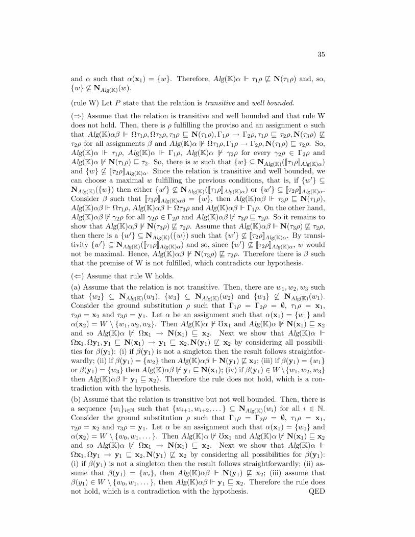
(rule W) Let P state that the relation is transitive and well bounded.
(⇒) Assume that the relation is transitive and well bounded and that rule Wdoes not hold. Then, there is ρ fulfilling the proviso and an assignment α suchthat Alg(K)αβ ° Ωτ1ρ,Ωτ3ρ, τ3ρ v N(τ1ρ), Γ1ρ → Γ2ρ, τ1ρ v τ2ρ,N(τ3ρ) 6vτ2ρ for all assignments β and Alg(K)α 6° Ωτ1ρ, Γ1ρ → Γ2ρ,N(τ1ρ) v τ2ρ. So,Alg(K)α ° τ1ρ, Alg(K)α ° Γ1ρ, Alg(K)α 6° γ2ρ for every γ2ρ ∈ Γ2ρ andAlg(K)α 6° N(τ1ρ) v τ2. So, there is w such that w ⊆ NAlg(K)([[τ1ρ]]Alg(K)α)and w 6⊆ [[τ2ρ]]Alg(K)α. Since the relation is transitive and well bounded, wecan choose a maximal w fulfilling the previous conditions, that is, if w′ ⊆NAlg(K)(w) then either w′ 6⊆ NAlg(K)([[τ1ρ]]Alg(K)α) or w′ ⊆ [[τ2ρ]]Alg(K)α.Consider β such that [[τ3ρ]]Alg(K)αβ = w, then Alg(K)αβ ° τ3ρ v N(τ1ρ),Alg(K)αβ ° Ωτ1ρ, Alg(K)αβ ° Ωτ3ρ and Alg(K)αβ ° Γ1ρ. On the other hand,Alg(K)αβ 6° γ2ρ for all γ2ρ ∈ Γ2ρ and Alg(K)αβ 6° τ3ρ v τ2ρ. So it remains toshow that Alg(K)αβ 6° N(τ3ρ) 6v τ2ρ. Assume that Alg(K)αβ ° N(τ3ρ) 6v τ2ρ,then there is a w′ ⊆ NAlg(K)(w) such that w′ 6⊆ [[τ2ρ]]Alg(K)α. By transi-tivity w′ ⊆ NAlg(K)([[τ1ρ]]Alg(K)α) and so, since w′ 6⊆ [[τ2ρ]]Alg(K)α, w wouldnot be maximal. Hence, Alg(K)αβ 6° N(τ3ρ) 6v τ2ρ. Therefore there is β suchthat the premise of W is not fulfilled, which contradicts our hypothesis.
(⇐) Assume that rule W holds.(a) Assume that the relation is not transitive. Then, there are w1, w2, w3 suchthat w2 ⊆ NAlg(K)(w1), w3 ⊆ NAlg(K)(w2) and w3 6⊆ NAlg(K)(w1).Consider the ground substitution ρ such that Γ1ρ = Γ2ρ = ∅, τ1ρ = x1,τ2ρ = x2 and τ3ρ = y1. Let α be an assignment such that α(x1) = w1 andα(x2) = W \ w1, w2, w3. Then Alg(K)α 6° fx1 and Alg(K)α 6° N(x1) v x2
and so Alg(K)α 6° Ωx1 → N(x1) v x2. Next we show that Alg(K)α °Ωx1,Ωy1,y1 v N(x1) → y1 v x2,N(y1) 6v x2 by considering all possibili-ties for β(y1): (i) if β(y1) is not a singleton then the result follows straightfor-wardly; (ii) if β(y1) = w2 then Alg(K)αβ ° N(y1) 6v x2; (iii) if β(y1) = w1or β(y1) = w3 then Alg(K)αβ 6° y1 v N(x1); (iv) if β(y1) ∈ W \w1, w2, w3then Alg(K)αβ ° y1 v x2). Therefore the rule does not hold, which is a con-tradiction with the hypothesis.(b) Assume that the relation is transitive but not well bounded. Then, there isa sequence wii∈N such that wi+1, wi+2, . . . ⊆ NAlg(K)(wi) for all i ∈ N.Consider the ground substitution ρ such that Γ1ρ = Γ2ρ = ∅, τ1ρ = x1,τ2ρ = x2 and τ3ρ = y1. Let α be an assignment such that α(x1) = w0 andα(x2) = W \ w0, w1, . . . . Then Alg(K)α 6° fx1 and Alg(K)α 6° N(x1) v x2
and so Alg(K)α 6° Ωx1 → N(x1) v x2. Next we show that Alg(K)α °Ωx1,Ωy1 → y1 v x2,N(y1) 6v x2 by considering all possibilities for β(y1):(i) if β(y1) is not a singleton then the result follows straightforwardly; (ii) as-sume that β(y1) = wi, then Alg(K)αβ ° N(y1) 6v x2; (iii) assume thatβ(y1) ∈ W \ w0, w1, . . . , then Alg(K)αβ ° y1 v x2. Therefore the rule doesnot hold, which is a contradiction with the hypothesis. QED

36
Observe that the characterization theorem above shows that the rules pro-posed in Subsection 2.6 characterize the envisaged properties of the accessibilityrelation even among general Kripke structures.
We now turn our attention to soundness and completeness of the modalsequent calculi over the general Kripke semantics. Soundness is easy to obtain,but, in order to establish completeness, we have to start by showing how toextract a general Kripke structure from a ΣK-algebra appropriate for the se-quent rules of a modal system. Recall that ΣK = 〈C,O, X, Y, Z〉 is the modalsignature introduced in Subsection 2.5.
Let A = 〈F, T, ·A〉 be a ΣK-algebra. Consider Kpk(A) = 〈W,Ã,B, V 〉where:
• W = ΩA
• t à t′ iff t′ vA NA(t);
• B = 〈f〉A : f ∈ F where 〈f〉A denotes the set t ∈ ΩA : t ≤A f;• V (pi) = 〈piA〉A.
In the sequel, we may write 〈f〉 for 〈f〉A when the underlying algebra isclear from the context.
Proposition 3.19 Given a ΣK-algebra A appropriate for CK , the tuple Kpk(A)is a general Kripke structure over C.
Proof:
(1) W is non empty. Indeed, by absurd, assume that W = ΩA = ∅. Then, sinceA is appropriate for rules cons and Ω, we would conclude that > ∈ ΩA.
(2) W ∈ B. Indeed, W = 〈[[t]]A〉 since A is appropriate for rule Rt.
(3) B is closed for complements. More precisely, we have to show that if 〈f〉 ∈ Bthen (W \ 〈f〉) ∈ B. Observe that W \ 〈f〉 = t ∈ W : t 6≤A f. We show belowthat t ∈ W : t 6≤A f = t ∈ W : t ≤A ¬A(f). Thus, the result follows sincethe latter set is 〈¬A(f)〉 which is in B.(i) t ∈ W : t 6≤A f ⊆ t ∈ W : t ≤A ¬A(f). Indeed, assume that t 6≤Af whenever t ∈ ΩA. So, by definition of satisfaction, choosing α such thatα(x1) = t and α(z1) = f , we have Aα ° Ωx1 → x1 6≤ z1. Observe thatΩx1 → x1 6≤ z1 `CK
Ωx1 → x1 ≤ ¬ z1:
1 Ωx1 → x1 ≤ ¬ z1 R¬ : 2
2 x1 ≤ z1, Ωx1 → LxeF : 3
3 Ωx1 → x1 6≤ z1 hyp
Therefore, by Theorem 3.4, Ωx1 → x1 6≤ z1 ²app(CK) Ωx1 → x1 ≤ ¬ z1. Hence,Aα ° Ωx1 → x1 ≤ ¬ z1. Again by definition of satisfaction and taking intoaccount the choice of α, we get t ≤A ¬A(f) whenever t ∈ ΩA.(ii) t ∈ W : t 6≤A f ⊇ t ∈ W : t ≤A ¬A(f). The proof is similar taking intoaccount Ωx1 → x1 ≤ ¬ z1 `CK
Ωx1 → x1 6≤ z1:

37
1 Ωx1 → x1 6≤ z1 cutF : 2, 3
2 Ωx1 → x1 6≤ z1,x1 ≤ ¬ z1 RwF : 4
3 x1 ≤ ¬ z1, Ωx1 → x1 6≤ z1 L¬ : 5
4 Ωx1 → x1 ≤ ¬ z1 hyp
5 Ωx1 → x1 6≤ z1,x1 ≤ z1 RxiF : 6
6 x1 ≤ z1, Ωx1 → x1 ≤ z1 ax
(4) B is closed for unions. More precisely, we have to show that if 〈f〉, 〈g〉 ∈ Bthen (〈f〉 ∪ 〈g〉) ∈ B. Observe that 〈f〉 ∪ 〈g〉 = t ∈ W : t ≤A f or t ≤A g. Weshow below that t ∈ W : t ≤A f or t ≤A g = t ∈ W : t ≤A ∨A(f, g). Thus,the result follows since the latter set is 〈∨A(f, g)〉 which is in B.(i) t ∈ W : t ≤A f or t ≤A g ⊆ t ∈ W : t ≤A ∨A(f, g). Indeed, assume thatt ≤A f or t ≤A g whenever t ∈ ΩA. So, by definition of satisfaction, choosingα such that α(x1) = t, α(z1) = f and α(z2) = g we have Aα ° Ωx1 → x1 ≤z1,x1 ≤ z2. Observe that Ωx1 → x1 ≤ z1,x1 ≤ z2 `CK
Ωx1 → x1 ≤ (z1 ∨ z2)by rule R∨. Therefore, by Theorem 3.4, Ωx1 → x1 ≤ z1,x1 ≤ z2 ²app(CK)
Ωx1 → x1 ≤ (z1 ∨ z2). Hence, Aα ° Ωx1 → x1 ≤ (z1 ∨ z2). Again by definitionof satisfaction and taking into account the choice of α, we get t ≤A ∨A(f, g)whenever t ∈ ΩA.(ii) t ∈ W : t ≤A f or t ≤A g ⊇ t ∈ W : t ≤A ∨A(f, g). The proof is similartaking into account Ωx1 → x1 ≤ (z1 ∨ z2) `CK
Ωx1 → x1 ≤ z1,x1 ≤ z2:
1 Ωx1 → x1 ≤ z1
x1 ≤ z2cutF : 2, 3
2 Ωx1 →x1 ≤ (z1 ∨ z2)x1 ≤ z1
x1 ≤ z2
RwF : 4
3x1 ≤ (z1 ∨ z2)Ωx1
→ x1 ≤ z1
x1 ≤ z2L∨ : 5, 6
4 Ωx1 → x1 ≤ (z1 ∨ z2) hyp
5x1 ≤ z1
Ωx1→ x1 ≤ z1
x1 ≤ z2ax
6x1 ≤ z2
Ωx1→ x1 ≤ z1
x1 ≤ z2ax
(5) B is closed for necessitations. More precisely, denoting by L(〈f〉) the sett ∈ W : t à t′ implies t′ ∈ 〈f〉 for every t′ ∈ W, we have to show that if 〈f〉 ∈B then L(〈f〉) ∈ B. Observe that L(〈f〉) = t ∈ W : t′ vA NA(t) implies t′ ∈〈f〉 for every t′ ∈ W = t ∈ W : t′ vA NA(t) implies t′ ≤A f for every t′ ∈W. We show below the latter set is equal to t ∈ W : t ≤A ¤A(f). Thus, theresult follows since the latter set is 〈¤A(f)〉 which is in B.(i) L(〈f〉) ⊆ t ∈ W : t ≤A ¤A(f). Indeed, assume that if t ∈ ΩA then forevery t′ ∈ ΩA we have t′ ≤A f whenever t′ vA NA(t). So, by definition ofsatisfaction, choosing α such that α(x1) = t and α(z1) = f , we have
Aα ° Ωx1, Ωy1,y1 v N(x1) → y1 ≤ z1 .
Observe that Ωx1, Ωy1,y1 v N(x1) → y1 ≤ z1 `CKΩx1 → x1 ≤ ¤z1 by
rules R¤ and Rgen. Therefore, by Theorem 3.4 Ωx1, Ωy1,y1 v N(x1) →

38
y1 ≤ z1 ²app(CK) Ωx1 → x1 ≤ ¤z1. Hence, Aα ° Ωx1 → x1 ≤ ¤z1. Againby definition of satisfaction and taking into account the choice of α, we gett ≤A ¤A(f) whenever t ∈ ΩA.(ii) L(〈f〉) ⊇ t ∈ W : t ≤A ¤A(f). The proof is similar taking into accountΩx1 → x1 ≤ ¤z1 `CK
Ωx1, Ωy1,y1 v N(x1) → y1 ≤ z1:
1Ωx1
Ωy1
y1 v N(x1)→ y1 ≤ z1 cutF : 2, 3
2Ωx1
Ωy1
y1 v N(x1)→ x1 ≤ z1
y1 ≤ z1w : 4
3
x1 ≤ z1
Ωx1
Ωy1
y1 v N(x1)
→ y1 ≤ z1 L : 5, 6, 7
4 Ωx1 → x1 ≤ z1 hyp
5
Ωy1
x1 ≤ z1
Ωx1
Ωy1
y1 v N(x1)
→ y1 v N(x1)y1 ≤ z1
ax
6
Ωy1
y1 ≤ z1
x1 ≤ z1
Ωx1
Ωy1
y1 v N(x1)
→ y1 ≤ z1 ax
7
x1 ≤ z1
Ωx1
Ωy1
y1 v N(x1)
→ Ωy1
y1 ≤ z1ax
QED
The following results show that the semantics of ground simple formulae ispreserved when we move from a ΣK-algebra appropriate for CK to the corre-sponding general Kripke structure.
Lemma 3.20 Let A be a ΣK-algebra appropriate for CK . Then, for everyground simple formula ϕ, 〈[[ϕ]]A〉 = [[ϕ]]Kpk(A).
Proof:
The proof is carried out by induction on the complexity of ϕ:
(Base) We have to consider only two representative cases:(i) ϕ is f . Then: 〈[[f ]]A〉 = 〈fA〉 = u ∈ ΩA : u ≤A fA which coincideswith u ∈ ΩA : u vA ⊥A since A is appropriate for rule Rf . Moreover,u ∈ ΩA : u vA ⊥A = ∅ since A is appropriate for rule Ω⊥. Therefore,〈[[f ]]A〉 = fKpk(A) = [[f ]]Kpk(A).(ii) ϕ is pi. Then: 〈[[pi]]A〉 = 〈piA〉 = V (pi) = [[pi]]Kpk(A).
(Step) We have to consider only three representative cases:(i) ϕ is ¬ϕ′. Then: 〈[[¬ϕ′]]A〉 = 〈¬A([[ϕ′]]A)〉 = u ∈ ΩA : u ≤A ¬A([[ϕ′]]A)

39
which coincides with u ∈ ΩA : u 6≤A [[ϕ′]]A as seen in part (2) of the proofof Proposition 3.19. Therefore, 〈[[¬ϕ′]]A〉 = ΩA \ u ∈ ΩA : u ≤A [[ϕ′]]A =ΩA \〈[[ϕ′]]A〉 which, by the induction hypothesis, is equal to ΩA \ [[ϕ′]]Kpk(A) and,so, identical to [[¬ϕ′]]Kpk(A).(ii) ϕ is ¤ϕ′. Then: 〈[[¤ϕ′]]A〉 = 〈¤A([[ϕ′]]A)〉 = u ∈ ΩA : u ≤A ¤A([[ϕ′]]A)which coincides with L(〈[[ϕ′]]A〉) as seen in part (4) of the proof of Proposi-tion 3.19. Therefore, by the induction hypothesis,〈[[¤ϕ′]]A〉 = L([[ϕ′]]Kpk(A))and, so, identical to [[¤ϕ′]]Kpk(A).(iii) ϕ is ϕ′∨ϕ′′. Then: 〈[[ϕ′ ∨ ϕ′′]]A〉 = 〈∨A([[ϕ′]]A, [[ϕ′′]]A)〉 which coincides withu ∈ ΩA : u ≤A [[ϕ′]]A or u ≤A [[ϕ′′]]A as seen in part (3) of the proof of Propo-sition 3.19. Therefore, 〈[[ϕ′ ∨ ϕ′′]]A〉 = u ∈ ΩA : u ≤A [[ϕ′]]A ∪ u ∈ ΩA : u ≤A[[ϕ′′]]A which, by the induction hypothesis, is equal to [[ϕ′]]Kpk(A) ∪ [[ϕ′′]]Kpk(A)
and, so, identical to [[ϕ′ ∨ ϕ′′]]Kpk(A). QED
Proposition 3.21 Given a ΣK-algebra A appropriate for CK and a groundsimple formula ϕ, A ° > ≤ ϕ iff Kpk(A) ° ϕ.
Proof:
(⇒) Assume A ° > ≤ ϕ. Then, >A ≤A [[ϕ]]A. Since A is appropriate for rules> and transF, for every t ∈ T , t ≤A [[ϕ]]A. In particular, for every u ∈ ΩA,u ≤A [[ϕ]]A. Therefore, u ∈ ΩA : u ≤A [[ϕ]]A = ΩA. Thus, 〈[[ϕ]]A〉 = ΩA and,so, [[ϕ]]Kpk(A) = W which means Kpk(A) ° ϕ.(⇐) Assume Kpk(A) ° ϕ. Then, u ∈ ΩA : u ≤A [[ϕ]]A = ΩA. Thus, since A isappropriate for rule Ω>, >A ≤A [[ϕ]]A, and, so, A ° > ≤ ϕ. QED
Proposition 3.22 Given a ΣK-algebra A appropriate for CK , an assignment βover A such that β(y1) = u ∈ ΩA and a ground simple formula ϕ, Aαβ ° y1 ≤ ϕiff Kpk(A)u ° ϕ.
Proof: Aαβ ° y1 ≤ ϕ iff β(y1) ≤A [[ϕ]]A iff u ∈ 〈[[ϕ]]A〉A iff u ∈ [[ϕ]]Kpk(A) iffKpk(A)u ° ϕ. QED
Given a class A of ΣK-algebras appropriate for the sequent rules of modalsystem K, let Kpk(A) be the class Kpk(A) : A ∈ A.Theorem 3.23 Given a class A of ΣK-algebras appropriate for CK :
• ψ1, . . . , ψk ²gA ϕ iff ψ1, . . . , ψk ²g
Kpk(A) ϕ;
• ψ1, . . . , ψk ²`A ϕ iff ψ1, . . . , ψk ²`
Kpk(A) ϕ.
Proof: Immediate using the two propositions above. QED
We are now ready to establish the counterpart of Theorem 3.18.
Theorem 3.24 (Cocharacterization) For each property P of the accessibil-ity relation and each ΣK-algebra A appropriate for CK :
Kpk(A) ∈ KP iff A ∈ app(CP ) .

40
Proof: Straightforward for each of the properties in Subsection 2.6. For in-stance, let P state that the relation is irreflexive. Then: Kpk(A) ∈ KP iff u 6Ã ufor every u ∈ W = ΩA iff u 6vA NA(u) for every u ∈ W . So, we have to showthat the latter holds iff, for every Γ1, Γ2, ρ, α, β, Aαβ ° Ωτ1ρ,Γ1ρ → Γ2ρ, τ1ρ 6vN(τ1ρ). QED
And, finally, we are now able to prove the envisaged completeness resultover general Kripke semantics.
Theorem 3.25 (Modal Kripke soundness and completeness) For each fi-nite set P of properties of the accessibility relation:
• ψ1, . . . , ψk ²gKP ϕ iff ψ1, . . . , ψk `g
CP ϕ;
• ψ1, . . . , ψk ²`KP ϕ iff ψ1, . . . , ψk ``
CP ϕ.
Proof:
(Soundness) Immediate by induction on the length of the derivation using (⇒)of Theorem 3.18, Theorem 3.17 and Theorem 3.16.
(Global completeness) Assume that ψ1, . . . , ψk 6 `gCP ϕ. Then, by Corollary 3.12,
ψ1, . . . , ψk 6 ²gapp(CP ) ϕ. That is, there is A ∈ app(CP) such that A ° > ≤ ψi for
i = 1, . . . , k and A 6° > ≤ ϕ. Let A be such an algebra and K = Kpk(A). Then,by Theorem 3.24, we know that K ∈ KP . Furthermore, by Proposition 3.21,K ° ψi for i = 1, . . . , k and K 6° ϕ. Therefore, ψ1, . . . , ψk 6 ²g
KP ϕ.
(Local completeness) Assume that ψ1, . . . , ψk 6 ``CP ϕ. Then, by Proposition 2.4,
6 `gCP (ψ1 ∧ . . . ∧ ψk) ⇒ ϕ. So, by global completeness as proved above, 6 ²g
KP(ψ1 ∧ . . . ∧ ψk)⇒ ϕ. Therefore, by Proposition 3.5, ψ1, . . . , ψk 6 ²`
KP ϕ. QED
It is straightforward to adapt the results in this subsection (about CK andits extensions) to the hybrid calculi introduced in Subsection 2.7.
We refrain to develop the details on this side issue, but it is worthwhile tocomment on the nature of Kpk(A) when A is appropriate for C@
K . Since, FAcontains elements representing all elements of ℘W , B collapses into ℘W in theresulting Kripke structure. Therefore, denoting by sKP the class of all standardKripke structures with set P of properties imposed on the accessibility relation,the theorem above becomes:
Theorem 3.26 For each finite set P of properties of the accessibility relation:
• ψ1, . . . , ψk ²gsKP ϕ iff ψ1, . . . , ψk `g
C@P
ϕ;
• ψ1, . . . , ψk ²`sKP ϕ iff ψ1, . . . , ψk ``
C@P
ϕ.
41
3.4 Duality between sober algebras and Kripke structures
In the previous subsection, we saw how to extract a ΣK-algebra appropriate forCK from a general Kripke structure and vice versa. It is natural to ask what isthe relationship, if any, between A and Alg(Kpk(A)) and also between K andKpk(Alg(K)). In order to answer these questions, first we need to set up thecategory of Σk-algebras and the category of general Kripke structures.
Recall that a p-morphism h : 〈W,Ã,B, V 〉 → 〈W ′, Ã′,B′, V ′〉 is a maph : W → W ′ such that:
a) if w1 Ã w2 then h(w1) Ã′ h(w2);
b) if h(w1) Ã′ w′2 then there is w2 such that h(w2) = w′2 and w1 Ã w2;
c) h−1(B′) ∈ B for every B′ ∈ B′;d) w ∈ V (pi) iff h(w) ∈ V ′(pi).
General Kripke structures together with p-morphisms constitute the cate-gory K. Observe that condition d) is equivalent to
d′) V (pi) = h−1(V ′(pi)).
In order to set up the envisaged category of ΣK-algebras appropriate forCK , we propose the following notion of morphism between such algebras. Tothis end, we need the following notation:
• f1 ∼A f2 iff 〈f1〉A = 〈f2〉A, that is, iff u ∈ ΩA : u ≤A f1 = u ∈ ΩA :u ≤A f2;
• dteA = u ∈ ΩA : u vA t;• t1 ≈A t2 iff t1 vA t2 and t2 vA t1, that is, iff dt1eA = dt2eA.
A morphism h : 〈F, T, ·A〉 → 〈F ′, T ′, ·A′〉 is a pair 〈−→h ,←−h 〉 where:
• −→h : F → F ′;
• ←−h : T ′ → T ;
such that
1)−→h (cA(f1, . . . , fk)) ∼A′ cA′(
−→h (f1), . . . ,
−→h (fk));
2) d←−h (t′)eA ⊆←−h (dt′eA′);
3)←−h (⊥A′) vA ⊥A;
4) NA(←−h (t′)) ≈A
←−h (NA′(t′));
5) if t′ ∈ ΩA′ then←−h (t′) ∈ ΩA;
6) if t′1 vA′ t′2 then←−h (t′1) vA
←−h (t′2);
42
7)←−h (t′) ≤A f iff t′ ≤A′
−→h (f) whenever t′ ∈ ΩA′ .
It is straightforward to verify that the ΣK-algebras appropriate for CK togetherwith these morphisms constitute a category that we denote by A.
This notion of morphism is sufficiently strong to ensure the preservationand reflection of satisfaction of labelled formula. To this end, it is convenientto make explicit the structure of an unbound variable assignment α over aΣ-algebra by identifying each such α with the pair 〈α|X , α|Z〉.
Theorem 3.27 (Satisfaction condition) Let h : A → A′ be a morphism,θ ∈ gT(ΣK) without bounded variables, ϕ ∈ gF(ΣK), α an unbounded variableassignment over A, and α′ an unbounded variable assignment over A′. Then:
A〈←−h α′|X , α|Z〉 ° θ ≤ ϕ iff A′〈α′|X ,−→h α|Z〉 ° θ ≤ ϕ .
Proof: The following two equalities can be proved by induction on the com-plexity of θ and ϕ, respectively:
1. [[θ]]A←−h α′|X =←−h ([[θ]]A′α′|X );
2.−→h ([[ϕ]]Aα|Z ) = [[ϕ]]A′−→h α|Z .
Now we have: A〈←−h α′|X , α|Z〉 ° θ ≤ ϕ iff [[θ]]A←−h α′|X ≤A [[ϕ]]Aα|Z iff (by 1.)←−h ([[θ]]A′α′|X ) ≤A [[ϕ]]Aα|Z iff (by property 7 of h) [[θ]]A′α′|X ≤A′
−→h ([[ϕ]]Aα|Z ) iff
(by 2.) [[θ]]A′α′|X ≤A′ [[ϕ]]A′−→h α|Z iff A′〈α′|X ,−→h α|Z〉 ° θ ≤ ϕ. QED
Corollary 3.28 Let h : A → A′ be a morphism, θ ∈ cgT(ΣK) and ϕ ∈cgF(ΣK). Then:
A ° θ ≤ ϕ iff A′ ° θ ≤ ϕ .
We now turn our attention towards extending the maps Alg and Kpk tofunctors.
Proposition 3.29 Given a p-morphism h : K → K′, the pair 〈h−1, h〉 is amorphism from Alg(K′) → Alg(K).
Proof:
1) h−1(cAlg(K′)(B′1, . . . , B
′k)) = cAlg(K)(h−1(B′
1), . . . , h−1(B′
k)) is established foreach representative modal constructor:(f) h−1(fAlg(K′)) = h−1(∅) = ∅ = fAlg(K).(pi) h−1(piAlg(K′)) = h−1(V ′(pi)) which by condition d′) is identical to V (pi) =piAlg(K).(¬) h−1(¬Alg(K′)(B′)) = h−1(W ′ \B′) = W \ h−1(B′) = ¬Alg(K)(h−1(B′)).(¤) h−1(¤Alg(K′)(B′)) = h−1(w′ : NAlg(K′)(w′) ⊆ B′) which is identicalto w : NAlg(K′)(h(w)) ⊆ B′ which thanks to 4) below coincides with w :h(NAlg(K)(w)) ⊆ B′ = w : NAlg(K)(w) ⊆ h−1(B′) = ¤Alg(K)(h−1(B′)).
43
(∨) h−1(∨Alg(K′)(B′1, B
′2)) = h−1(B′
1 ∪ B′2) which coincides with h−1(B′
1) ∪h−1(B′
2) = ∨Alg(K)(h−1(B′1), h
−1(B′2)).
2) dh(U)eAlg(K′) = h(dUeAlg(K)). Indeed, dh(U)eAlg(K′) = u′ : u′ ∈ h(U) =h(u) : u ∈ U = h(u : u ∈ U) = h(dUeAlg(K)).
3) h(∅) vAlg(K′) ∅. Indeed: h(∅) = ∅.4) NAlg(K′)(h(U)) = h(NAlg(K)(U)). Indeed:(⊆) Consider any w′ ∈ NAlg(K′)(h(U)). Then, by definition of Alg(K′), there isu ∈ U such that h(u) Ã′ w′. So, by property b) of the p-morphism, there isw ∈ W such that h(w) = w′ and u à w. That is, thanks to the definition ofAlg(K), w ∈ NAlg(K)(u) and, therefore, h(w) = w′ is in h(NAlg(K)(U)).(⊇) Consider any w ∈ NAlg(K)(U). Then, there is u ∈ U such that u Ãw. So, by property a) of the p-morphism, h(u) Ã′ h(w). Hence, h(w) ∈NAlg(K′)(h(U)).Since Alg(K′) is appropriate for rule ref, we obtain NAlg(K′)(h(U)) vAlg(K′)h(NAlg(K)(U)) and h(NAlg(K)(U)) vAlg(K′) NAlg(K′)(h(U)).
5) h(w) ∈ ΩAlg(K′) for every w ∈ ΩAlg(K). Immediate: h(w) = h(w).6) h(U1) vAlg(K′) h(U2) for every U1 vAlg(K) U2. Immediate: h(U1) ⊆ h(U2)whenever U1 ⊆ U2.
7) h(w) ≤Alg(K′) B′ iff w ≤Alg(K) h−1(B′) for every w ∈ ΩAlg(K). Imme-diate: h(w) ∈ B′ iff w ∈ h−1(B′). QED
It is now straightforward to verify that the map Alg can be extended to afunctor from K to Aop. Furthermore, the map Kpk can also be extended to afunctor from Aop to K thanks to the following result.
Proposition 3.30 Given a morphism h : A′ → A, the map←−h |ΩA is a p-
morphism from Kpk(A) → Kpk(A′).
Proof:
a) For every t1, t2 ∈ W , if t1 Ã t2 then←−h |ΩA(t1) Ã′ ←−h |ΩA(t2). Indeed: Assume
that t1 Ã t2. Then, by definition of Kpk(A), t2 vA NA(t1). So, by property 6)of the algebra morphism,
←−h |ΩA(t2) vA′
←−h |ΩA(NA(t1)). Hence, by property 4) of
the algebra morphism and since A′ is appropriate for rule transT,←−h |ΩA(t2) vA′
NA′(←−h |ΩA(t1)). That is, by definition of Kpk(A′),
←−h |ΩA(t1) Ã′ ←−h |ΩA(t2).
b) For every t1 ∈ W and t′2 ∈ W ′, if←−h |ΩA(t1) Ã′ t′2 then there is t2 ∈ W such
that←−h |ΩA(t2) = t′2 and t1 Ã t2. Indeed: Assume
←−h |ΩA(t1) Ã′ t′2. Then, by con-
struction of Kpk(A′), t′2 vA′ NA′(←−h |ΩA(t1)). So, by property 4) of the algebra
morphism and since A′ is appropriate for rule transT, t′2 ∈ d←−h |ΩA(NA(t1))eA′
and, therefore by property 2) of the algebra morphism, t′2 ∈←−h |ΩA(dNA(t1)eA).
Thus, there is t2 ∈ dNA(t1)eA such that←−h |ΩA(t2) = t′2. That is, there is
t2 vA NA(t1) such that←−h |ΩA(t2) = t′2. Or, equivalently, there is t2 ∈ W such
44
that t1 Ã t2 and←−h |ΩA(t2) = t′2.
c) For each f ′ ∈ F ′, (←−h |ΩA)
−1(〈f ′〉) ∈ B. Indeed, (
←−h |ΩA)
−1(〈f ′〉) is the set
u ∈ ΩA :←−h |ΩA(u) ≤A′ f ′ which coincides, thanks to property 7) of the al-
gebra morphism, with u ∈ ΩA : u ≤A−→h (f ′). The latter set is by definition
〈−→h (f ′)〉 which belongs to B.
d′) V (pi) = (←−h |ΩA)
−1(V ′(pi)). Indeed, (
←−h |ΩA)
−1(V ′(pi)) = (
←−h |ΩA)
−1(〈piA′〉)
which, following the same reasoning as in c) above, is 〈−→h (piA′)〉 and, so, byproperty 1) of the algebra morphism, is identical to 〈piA〉 which coincides withV (pi). QED
We are now ready to address the questions stated at the beginning of thissubsection. The relationship between K and Kpk(Alg(K)) is easy to establish.
Proposition 3.31 Let K be a general Kripke structure. Then, K is isomorphicin K to Kpk(Alg(K)).
Proof: Consider the map h : WK → WKpk(Alg(K)) such that h(w) = w. It isstraightforward to show that it is a p-morphism. Furthermore, h is a bijectivemap and its inverse is also a p-morphism. QED
On the other hand, the relationship between A and Alg(Kpk(A)) is not sosimple. Indeed, the best that we can do is to establish an adjunction between Kand the dual of the subcategory of A containing the ΣK-algebras appropriatefor CK where ∼ / ≈ is the diagonal relation in F/T , respectively. More precisely,a ΣK-algebra is said to be sober iff:
• f1 ∼A f2 iff f1 = f2;
• t1 ≈A t2 iff t1 = t2.
The full subcategory of A with all sober algebras is denoted by sA. It isstraightforward to establish the inclusion functor I : sA → A. In the oppositedirection, the quotient functor Q : A → sA can be obtained by the compositionQ2 Q1 where:
• Q1 : A → sA, denoting by sA the full subcategory of A with all algebrasthat are sober with respect to ∼ (but not necessarily with respect to ≈),defined as follows:
– Q1(A) = 〈F/ ∼A, T, ·Q1(A)〉 where:
∗ cQ1(A)([f1]∼A , . . . , [fk]∼A) = [cA(f1, . . . , fk)]∼A ;∗ oQ1(A) = oA;∗ ΩQ1(A) = ΩA;∗ vQ1(A)=vA;∗ ≤Q1(A)= 〈t, [f ]∼A〉 : 〈t, f〉 ∈≤A.

45
Note that Q1(A) is well defined since ∼A is a congruence relation.
– Q1(h : A→ A′) : Q1(A) → Q1(A′) is the pair 〈−−−→Q1(h),←−h 〉 where:
∗ −−−→Q1(h)([f ]∼A) = [−→h (f)]∼A′ .
Observe that Q1(h) is well defined thanks to property 7) of h.
• Q2 : sA → sA defined as follows:
– Q2(A) = 〈F, T/ ≈A, ·Q2(A)〉 where:
∗ cQ2(A) = cA;∗ oQ2(A)([t1]≈A , . . . , [tk]≈A) = [oA(t1, . . . , tk)]≈A ;∗ ΩQ2(A) = [u]≈A : u ∈ ΩA;∗ vQ2(A)= 〈[t1]≈A , [t2]≈A〉 : 〈t1, t2〉 ∈vA;∗ ≤Q2(A)= 〈[t]≈A , f〉 : 〈t, f〉 ∈≤A.
Note that Q2(A) is well defined since ≈A is a congruence relation.
– Q2(h : A→ A′) : Q2(A) → Q2(A′) is the pair 〈−→h ,←−−−Q2(h)〉 where:
∗ ←−−−Q2(h)([t′]≈A′ ) = [←−h (t′)]≈A .
Observe that Q2(h) is well defined thanks to property 6) of h.
Let I1 : sA → A and I2 : sA → sA be the inclusion functors. Then, it isstraightforward to show that Q1 is left adjoint for I1 and Q2 is right adjointfor I2. Hence, sA is a coreflective subcategory of sA and sA is a reflectivecategory of A. So, Q corresponds to a canonical construction, in this case bycomposition of two universal constructions.
In fact, for the purposes of this paper, we could work within sA instead ofworking in A since the following result holds:
Proposition 3.32
Aαβ ° δ iff Q(A)([ ] α)([ ] β) ° δ .
Proof: The result follows straightforwardly, by noting that the two equalitieshold: [[[θ]]Aαβ]∼A = [[θ]]Q(A)([ ]α)([ ]β) and [[[ϕ]]Aα]≈A = [[ϕ]]Q(A)([ ]α). QED
Furthermore, observe that Alg(K) is in sA. So, the functor Alg : K → Ainduces a functor from K to sA that we denote by sAlg. Letting sKpk bethe restriction of functor Kpk to sA, we now establish the envisaged dualitybetween sober algebras and general Kripke structures.
We start by giving the “road map” of the proof of the theorem:
• we introduce a candidate morphism ηA : sAlgsKpk(A) → A for each A(the unit of the adjunction) namely proposing the definition of the truthvalue map ←−ηA and the formula map −→ηA;
• we show that ηA is a morphism in sAop (done in step (i)). According tothe definition this requires checking properties:

46
– −→ηA(csAlg(sKpk(A))(〈f1〉A, . . . , 〈fk〉A)) ∼A cA(f1, . . . , fk)(done in substep (1) for each constructor);
– d←−ηA(t)esAlg(sKpk(A)) ⊆ ←−ηA(dteA)(done in substep (2));
– ←−ηA(⊥A) vsAlg(sKpk(A)) ⊥sAlg(sKpk(A))
(done in substep (3));
– NsAlg(sKpk(A))(←−ηA(t)) ≈sAlg(sKpk(A))
←−ηA(NA(t))(done in substep (4));
– if t ∈ ΩA then ←−ηA(t) ∈ ΩsAlg(sKpk(A))
(done in substep (5));
– if t1 vA t2 then ←−ηA(t1) vsAlg(sKpk(A))←−ηA(t2)
(done in substep (6));
– ←−ηA(t) ≤sAlg(sKpk(A)) 〈f〉A iff t ≤A −→ηA(〈f〉A) whenever t ∈ ΩA
(done in substep (7));
• we show the universal property: given any K′ in K and any morphismh : A→ sAlg(K′) in sAop, there is a unique morphism h′ : sKpk(A) → K′in K such that sAlg(h′) ηA = h (done in step (ii));
– definition of candidate morphism h′ (substep existence);
– we show that h′ is a a morphism in K:
∗ if w1 ÃsKpk(A) w2 then h′(w1) ÃK′ h′(w2)(done in substep (a));
∗ if h′(w1) ÃK′ w′2 then there is w2 such that h′(w2) = w′2 andw1 ÃsKpk(A) w2
(done in substep (b));∗ h′−1(B′) ∈ BsKpk(A) for every B′ ∈ BK′
(done in substep (c));∗ VsKpk(A)(pi) = h′−1(VK′(pi))
(done in substep (d’));
– we show the commutativity of the truth value maps;(done in substep (e));
– we show the commutativity of the formula maps;(done in substep (f));
– finally, we show the unicity of h′
(done in substep (unicity)).
Theorem 3.33 (Duality) Functor sKpk : sAop → K is left adjoint for func-tor sAlg : K → sAop.

47
Proof:
Let A = 〈F, T, ·A〉 be a sober ΣK-algebra. Denote the set 〈f〉A : f ∈ F by〈F 〉A. Consider the maps:
• −→ηA : 〈F 〉A → F defined as follows: −→ηA(〈f〉A) = f ;
• ←−ηA : T → ℘ΩA defined as follows: ←−ηA(t) = dteA.
(i) We first show that the pair ηA = 〈−→ηA,←−ηA〉 is a morphism in sAop from Ato sAlg(sKpk(A)). That is, ηA is a morphism in sA from sAlg(sKpk(A)) to A.Indeed:
(1) −→ηA(csAlg(sKpk(A))(〈f1〉A, . . . , 〈fk〉A)) ∼A cA(f1, . . . , fk) holds for each repre-sentative constructor:
(f) Observe that fsAlg(sKpk(A)) = ∅ by definition of sAlg. And so is 〈fA〉A be-cause A is appropriate for rules Rf and Ω⊥. Therefore: 〈−→ηA(fsAlg(sKpk(A)))〉A =〈−→ηA(∅)〉A = 〈−→ηA(〈fA〉A)〉A = 〈fA〉A.
(pi) Note that pisAlg(sKpk(A)) = VsKpk(A)(pi) by definition of sAlg. And thelatter is equal to 〈piA〉A by definition of sKpk. Thus: 〈−→ηA(pisAlg(sKpk(A)))〉A =〈−→ηA(VsKpk(A)(pi))〉A = 〈−→ηA(〈piA〉A)〉A = 〈piA〉A.
(¬) −→ηA(¬sAlg(sKpk(A))(〈f〉A)) = −→ηA(ΩA \ 〈f〉A) = −→ηA(u ∈ ΩA : u 6≤A f) which,as seen in part (3) of Proposition 3.19, is −→ηA(u ∈ ΩA : u ≤A ¬A(f)) =−→ηA(〈¬A(f)〉A) = ¬A(f) = ¬A(−→ηA(〈f〉A)).
(¤) −→ηA(¤sAlg(sKpk(A))(〈f〉A)) = −→ηA(u ∈ ΩA : NsAlg(sKpk(A))(u) ⊆ 〈f〉A) =−→ηA(v ∈ ΩA : u ÃsKpk(A) v implies v ∈ 〈f〉A) which, as seen in part (5) ofProposition 3.19, coincides with −→ηA(u ∈ ΩA : u ≤A ¤A(f)) and, therefore, isequal to −→ηA(〈¤A(f)〉A) = ¤A(f) = ¤A(−→ηA(〈f〉A)).
(∨) −→ηA(∨sAlg(sKpk(A))(〈f〉A, 〈g〉A)) = −→ηA(u ∈ ΩA : u ≤A f or u ≤A g) and, so,as in part (4) of Proposition 3.19, equal to −→ηA(u ∈ ΩA : u ≤A ∨A(f, g)) =−→ηA(〈∨A(f, g)〉A) = ∨A(f, g) = ∨A(−→ηA(〈f〉A),−→ηA(〈g〉A)).
(2) d←−ηA(t)esAlg(sKpk(A)) ⊆ ←−ηA(dteA). Indeed, assume u ∈ d←−ηA(t)esAlg(sKpk(A)).Therefore, u ∈ ΩA. Furthermore, u ⊆ ←−ηA(t). So, u ⊆ dteA. That is,u ∈ dteA and, so, u vA t. On the other hand, ←−ηA(dteA) = dveA : v ∈ΩA and v vA t which, since A is sober and appropriate for rule Rasym, isequal to v : v ∈ ΩA and v vA t which obviously contains u.(3) ←−ηA(⊥A) vsAlg(sKpk(A)) ⊥sAlg(sKpk(A)). Indeed, thanks to the definition ofsAlg, this assertion is equivalent to ←−ηA(⊥A) ⊆ ∅. Moreover, ←−ηA(⊥A) = u ∈ΩA : u vA ⊥A which is the empty set since A is appropriate for rule Ω⊥.
(4) NsAlg(sKpk(A))(←−ηA(t)) ≈sAlg(sKpk(A))
←−ηA(NA(t)). Indeed, the former set isequal to NsAlg(sKpk(A))(u ∈ ΩA : u vA t) which, by the definition of the twofunctors, coincides with v ∈ ΩA : there is u ∈ ΩA such that u vA t and v vANA(u). Finally, this set is equal to v ∈ ΩA : v vA NA(t) because A isappropriate for rules RNΩ and LNΩ.
(5) If t ∈ ΩA then ←−ηA(t) ∈ ΩsAlg(sKpk(A)). Indeed, assume t ∈ ΩA. Then,

48
←−ηA(t) = u ∈ ΩA : u vA t which is the singleton set t since t is atomicand A is sober and appropriate for rule Rasym. Therefore, ←−ηA(t) is atomic insAlg(sKpk(A)).
(6) If t1 vA t2 then ←−ηA(t1) vsAlg(sKpk(A))←−ηA(t2). Indeed, the latter assertion is
equivalent to u ∈ ΩA : u vb At1 ⊆ u ∈ ΩA : u vb At2. Assuming thatt1 vA t2, the assertion holds thanks to the fact that A is appropriate for ruletransT.
(7)←−ηA(t) ≤sAlg(sKpk(A)) 〈f〉A iff t ≤A −→ηA(〈f〉A) whenever t ∈ ΩA. Indeed, ←−ηA(t) =v ∈ ΩA : v vA t = t as seen in (5) above. So, ←−ηA(t) ≤sAlg(sKpk(A)) 〈f〉A ifft ⊆ 〈f〉A iff t ⊆ v ∈ ΩA : v ≤A f iff t ≤A f iff t ≤A −→ηA(〈f〉A).
(ii) We now show that the family η, where each ηA is the morphism in sAop
from A to sAlg(sKpk(A)) defined above, is the unit of the envisaged adjunc-tion. More precisely, we show that, given any K′ in K and any morphismh : A→ sAlg(K′) in sAop, there is a unique morphism h′ : sKpk(A) → K′ in Ksuch that sAlg(h′) ηA = h.
(existence) Consider h′ defined as follows: for each world w ∈ WsKpk(A) = ΩA,
h′(w) = ι(←−h (w)) =←−h (w). Observe that h′ is well defined because of prop-
erty 5) of h and the fact that the atomic elements in sAlg(K′) are the singletonsubsets of WK′ . First, we show that the map h′ is a morphism in K fromsKpk(A) to K′:
(a) If w1 ÃsKpk(A) w2 then h′(w1) ÃK′ h′(w2). Indeed, assume w1 ÃsKpk(A) w2.
Then, w2 vA NA(w1). So, by property 6) of morphism h,←−h (w2) vsAlg(K′)←−
h (NA(w1)). Hence, by property 4) of h,←−h (w2) vsAlg(K′) NsAlg(K′)(
←−h (w1)).
Hence, h′(w1) ÃK′ h′(w2).
(b) If h′(w1) ÃK′ w′2 then there is w2 such that h′(w2) = w′2 and w1 ÃsKpk(A)
w2. Indeed, from h′(w1) ÃK′ w′2 we conclude w′2 ⊆ NsAlg(K′)(h′(w1)), that
is, w′2 ⊆ NsAlg(K′)(←−h (w1)). Thus, by property 4) of h, w′2 ⊆
←−h (NA(w1))
and, so, w′2 ∈ d←−h (NA(w1))esAlg(K′). Hence, thanks to property 2) of h,
w′2 ∈ ←−h (dNA(w1)eA). Therefore, there is
←−h (w2) = w′2 such that w2 ∈
dNA(w1)eA. That is, there is←−h (w2) = w′2 such that w1 ÃsKpk(A) w2.
(c) h′−1(B′) ∈ BsKpk(A) for every B′ ∈ BK′ . Indeed, observe that h′−1(B′) =
w ∈ ΩA : h′(w) ∈ B′ = w ∈ ΩA :←−h (w) ⊆ B′. Using property 7) of h,
the latter set coincides with w ∈ ΩA : w vA−→h (B′) = 〈−→h (B′)〉A which is in
〈FA〉 = BsKpk(A).
(d′) VsKpk(A)(pi) = h′−1(VK′(pi)). Indeed, as seen in (c) above, h′−1(VK′(pi)) =
〈−→h (VK′(pi))〉A. The latter set, by definition of sAlg(K′), is 〈−→h (pisAlg(K′))〉Awhich, thanks to property 1) of h, coincides with 〈piA〉A and, so, with VsKpk(A)(pi).
We now verify that sAlg(h′) ηA = h:
(e)←−−−−−sAlg(h′)←−ηA =
←−h . Indeed, for each t ∈ TA,
←−−−−−sAlg(h′)(←−ηA(t)) =
←−−−−−sAlg(h′)(dteA).

49
Furthermore, by definition of sAlg(h′), the latter is h′(dteA). We show that, forevery w′ ∈ WK′ , w′ ∈ h′(dteA) iff w′ ∈ ←−h (t):
(⇒) Assume w′ ∈ h′(dteA). Then, there is u ∈ dteA such that h′(u) = w′. Thatis, there is u ∈ ΩA such that u vA t and
←−h (u) = w′. Thus, by property 6)
of h, there is u ∈ ΩA such that←−h (u) ⊆ ←−
h (t) and←−h (u) = w′. Therefore,
w′ ∈ ←−h (t).
(⇐) Assume w′ ∈ ←−h (t). That is, w′ ⊆ ←−h (t). Hence, w′ ∈ d←−h (t)esAlg(K′).
Thus, by property 3) of h, w′ ∈ ←−h (dteA) and, so, w′ ∈ h′(dteA).
(f) −→ηA−−−−−→sAlg(h′) =
−→h . Indeed, for each B′ ∈ FsAlg(K′) = BK′ , −→ηA(
−−−−−→sAlg(h′)(B′)) =
−→ηA(h′−1(B′)) = −→ηA(〈−→h (B′)〉A) =−→h (B′).
(unicity) Observe that there is a unique choice of h′ that ensures the diagramcomutes. Namely, h′ should be chosen in order to guarantee that
←−−−−−sAlg(h′)←−ηA =←−
h . So, in particular, for each w ∈ WsKpk(A) = ΩA, h′ should be chosen in order
to guarantee that h′(dweA) =−→h (w). That is, h′ should be chosen in order to
ensure h′(w) =−→h (w), that is, h′(w) =
−→h (w). Therefore, the choice of h′
is unique. QED
3.5 Analyticity of the modal sequent calculi
A rule r = 〈s1, . . . , sp, s, π〉 is said to be a creative rule if there are meta-variables in s1, . . . , sp that do not occur in s. Most of the structural, order andmodal rules introduced in Section 2 are non creative. The obvious exceptionsare:
• structural: cutT and cutF;
• order: Ω>, Ω, transT, transF, LgenT, RgenT, LgenF and RgenF;
• system K: LNΩ, RNΩ, L♦ and R♦;
• other modal systems: 5 and C.
We distinguish two kinds of creative rules. A creative rule is said to be ablindly creative rule if when applying the rule in a derivation, the instance ofthe additional meta-variable in the premises is chosen as a fresh variable (inour case a bounded truth value variable y). An example of a blindly creativerule is Ω>.
On the other hand, a creative rule is said to be a strongly creative rule ifwhen applying the rule in a derivation, the instance of the additional meta-variable in the premises is not necessarily a fresh variable. In the case of thesequent calculi at hand, we have the following strongly creative rules:
• structural: cutT and cutF;
• order: transT, transF, LgenT and LgenF;

50
• system K: RNΩ and R♦;
• other modal systems: 5.
A derivation 〈d1, π1〉, . . . , 〈dn, πn〉 of s′ from S is said to be analytical if theinstance of each additional meta-variable when applying strongly creative rulesat step i has to occur either in d1, . . . , di−1 or in S. A sequent calculus is said tobe analytical if all derivations are analytical. Clearly, our sequent calculus formodal logic is not analytical since it allows derivations that are not analytical.
The importance of this concept comes from the fact that derivations canbe automated. We can make our calculus analytic by keeping all non stronglycreative rule and introducing restrictive versions of strongly creative rules asfollows:
cutT• Γ1→Γ2,τ1vτ2 τ1vτ2,Γ1→Γ2Γ1→Γ2
C τ1, τ2 ∈ Γ1, Γ2
cutF• Γ1→Γ2,τ1≤ξ1 τ1≤ξ1,Γ1→Γ2Γ1→Γ2
C τ1, ξ1 ∈ Γ1,Γ2
transT• Γ1→Γ2,τ1vτ2 Γ1→Γ2,τ2vτ3Γ1→Γ2,τ1vτ3
C τ2 ∈ τ1, τ3, Γ1, Γ2
transF• Γ1→Γ2,τ1vτ2 Γ1→Γ2,τ2≤ξ1Γ1→Γ2,τ1≤ξ1
C τ2 ∈ τ1, Γ1, Γ2
LgenT• Ωτ2,τ2vτ3,Γ1→Γ2 Ωτ2,Γ1→Γ2,τ2vτ1 τ1vτ3,Γ1→Γ2,Ωτ2τ1vτ3,Γ1→Γ2
C τ2 ∈ τ1, τ3,Γ1,Γ2
LgenF• Ωτ2,τ2≤ξ1,Γ1→Γ2 Ωτ2,Γ1→Γ2,τ2vτ1 τ1≤ξ1,Γ1→Γ2,Ωτ2τ1≤ξ1,Γ1→Γ2
C τ2 ∈ τ1, Γ1, Γ2
RNΩ• Ωτ2,Γ1→Γ2,Ωτ3 Ωτ3,Ωτ2,Γ1→Γ2,τ3vτ1 Ωτ3,Ωτ2,Γ1→Γ2,τ2vN(τ3)Ωτ2,Γ1→Γ2,τ2vN(τ1)
C τ3 ∈ τ1, τ2, Γ1, Γ2
R♦• Ωτ1,Ωτ2,Γ1→Γ2,τ2vN(τ1) Ωτ1,Ωτ2,Γ1→Γ2,τ2≤ξ1 Ωτ1,Γ1→Γ2,Ωτ2Ωτ1,Γ1→Γ2,τ1≤(♦ξ1)
C τ2 ∈ τ1, Γ1, Γ2
5• Ωτ1,Ωτ2,Ωτ3,Γ1→Γ2,τ1vN(τ3) Ωτ1,Ωτ2,Ωτ3,Γ1→Γ2,τ2vN(τ3) Ωτ1,Ωτ2,Γ1→Γ2,Ωτ3Ωτ1,Ωτ2,Γ1→Γ2,τ1vN(τ2)
C τ3 ∈ τ1, τ2, Γ1, Γ2
where, for instance, the proviso (τ2 ∈ τ1,Γ1, Γ2)(ρ) = 1 iff ρ(τ2) occurs inρ(τ1) ∪ ρ(Γ1)∪ ρ(Γ2) or in the hypotheses. Clearly, the other provisos have asimilar meaning.
For each finite set P of properties of the accessibility relation considered inSubsection 2.6, let also C•P denote the restricted version of CP .
Can we guarantee that by restricting ourselves only to analytical applica-tions of these strongly creative rules nothing is lost? That is, the sequent calculiremain complete if we restrict the use of these rules?
Fortunately, the answer is positive. Indeed, careful examination of theproofs of the relevant metatheorems in Subsection 2.9 and of the complete-ness result in Subsection 3.2, shows that appropriateness for each of these ruleswas invoked only in its restricted form. As a consequence, we establish thefollowing extension of Theorem 3.11.
Theorem 3.34 (Algebraic completeness) Every full structural sequent cal-culus endowed with rules using only persistent provisos and restrictive versionsof cutT• and cutF• is complete.

51
Proof: Since this completeness result was established using strongly creativerules in their restricted form, the proof is the same as in Theorem 3.11. QED
This result can be further extended to sequent calculi for modal logic sincethe proofs in Subsection 3.3 only use strongly creative rules in their restrictiveform. As a consequence, we establish an extension of Theorem 3.25.
Theorem 3.35 (Modal Kripke soundness and completeness) For each fi-nite set P of properties of the accessibility relation:
• ψ1, . . . , ψk ²gKP ϕ iff ψ1, . . . , ψk `g
C•P ϕ;
• ψ1, . . . , ψk ²`KP ϕ iff ψ1, . . . , ψk ``
C•P ϕ.
Proof: We only show the global case since the local case is similar.
Assume that ψ1, . . . , ψk ²gKP ϕ, then by Theorem 3.25 we have ψ1, . . . , ψk `g
CPϕ. Since to establish the latter theorem we only used strongly creative rules intheir restrictive form, the same derivation can be used to establish ψ1, . . . , ψk `g
C•Pϕ. The converse is straightforward. QED
4 Concluding remarks
By using truth values as labels, we were able to provide analytical labelledsequent calculi for a wide class of normal modal systems sharing a common coreof rules (structural rules, order rules, and rules for the formula constructors).The calculus for each modal system is obtained by adding to this common corerules on the truth values imposing the envisaged properties of the accessibilityrelation. We also managed to keep an effective separation between the sub-calculus on the formulae and the sub-calculus on the truth values. Therefore,the way is open for proving desirable proof-theoretic properties of, at least,the formula sub-calculus like, for instance, the elimination of rule cutF (cf theresults in [19] where a similar separation was explored in the case of a naturaldeduction calculus labelled with worlds for obtaining normalization results).
These calculi were shown to be strongly complete (for both global and localreasoning) with respect to the novel two-sorted algebraic semantics, and, as acorollary, also with respect to the general Kripke semantics. For this purpose,we had to indicate how to move back and forth between such algebras andgeneral Kripke structures. This led to a duality between the category of soberalgebras and the category of general Kripke structures (with p-morphisms). Asimple enrichment of the language (by adding the coercion operator @) wasshown to allow reasoning complete with respect to standard Kripke structures.
It is worthwhile to comment on the nature of the two-sorted algebras. In asense they are halfway between general Kripke structures and modal algebras.We may look at them as general Kripke structures without points. The mainresults of the paper clearly show that the loss of the points was possible whilepreserving the ability to spell out the envisaged properties of the accessibility

52
relation. One might argue that we do keep points through the Ω predicate.To some extent this is a fair observation, but we should stress that the calculiimpose very little about the atomic truth values, for sure much less than whatis implied by set theory about singletons.
The proposed sequent calculi labelled with truth values are relevant to au-tomation and to the theory and applications of the combination of deductionsystems. Furthermore, the two-sorted algebraic semantics introduced hereinseems to achieve the right balance between modal algebras and Kripke struc-tures by sharing the advantages of both. Indeed, while algebraic in flavor, thisnew semantics still allows the specification of modal systems with rules reflect-ing the envisaged properties of the accessibility relation, fully characterizingthose systems even among general Kripke structures.
Capitalizing on the results of this paper, several lines of research are evi-dent at this stage. First, taking advantage of the separation between the for-mula sub-calculus and the truth value sub-calculus, there is hope of obtaininguseful proof-theoretic results about the proposed modal calculi (for instance,elimination of rule cutF and control of the application of other rules such ascontractions), towards making the calculi even more interesting from an au-tomation point of view. Second, extrapolating from the preliminary ideas inSubsection 2.7, the relationship to hybrid logic seems to be a fruitful line of re-search, for instance towards a hybrid logic over truth values (instead of worlds).Third, given the generality of the approach (well illustrated by the algebraiccompleteness theorem that requires very little from the calculus at hand), it isfeasible to set up sequent calculi labelled with truth values for other types oflogic (like intuitionistic, relevance, many-valued logics) and develop a theory offibring such calculi (where the general algebraic completeness result obtained inthis paper can be used in the style of [21, 17] for establishing the preservationof completeness by fibring).
Acknowledgments
This work was partially supported by Fundacao para a Ciencia e a Tecnolo-gia (FCT, Portugal), namely via the FEDER Project FibLog POCTI/MAT/37239/2001. The authors wish to express their gratitude to Carlos Areces, Alessan-dra Carbone, Walter Carnielli, Marcelo Finger and Joao Rasga for useful feed-back at different stages of this work. We are also grateful to the anonymousreferee for many valuable suggestions.
References
[1] P. Andrews. An introduction to mathematical logic and type theory: totruth through proof, volume 27 of Applied Logic Series. Kluwer AcademicPublishers, Dordrecht, second edition, 2002.

53
[2] Carlos Areces, Patrick Blackburn, and Maarten Marx. Hybrid logics:Characterization, interpolation and complexity. Journal of Symbolic Logic,66(3):977–1010, 2001.
[3] Matthias Baaz, Christian G. Fermuller, Gernot Salzer, and Richard Zach.Labeled calculi and finite-valued logics. Studia Logica, 61(1):7–33, 1998.
[4] David Basin, Sean Matthews, and Luca Vigano. Labelled propositionalmodal logics: theory and practice. Journal of Logic and Computation,7(6):685–717, 1997.
[5] P. Blackburn, M. de Rijke, and Y. Venema. Modal logic, volume 53 ofCambridge Tracts in Theoretical Computer Science. Cambridge UniversityPress, Cambridge, 2001.
[6] Patrick Blackburn. Internalizing labelled deduction. Journal of Logic andComputation, 10(1):137–168, 2000.
[7] Patrick Blackburn and M. Tzakova. Hybrid completeness. Logic Journalof the IGPL, 6:625–650, 1998.
[8] Krysia Broda, Marcelo Finger, and Alessandra Russo. Labelled naturaldeduction for substructural logics. Logic Journal of the IGPL, 7(3):283–318, 1999.
[9] Walter A. Carnielli. Systematization of finite many-valued logics throughthe method of tableaux. Journal of Symbolic Logic, 52(2):473–493, 1987.
[10] Marcello D’Agostino and Dov M. Gabbay. A generalization of analytic de-duction via labelled deductive systems I: Basic substructural logics. Jour-nal of Automated Reasoning, 13(2):243–281, 1994.
[11] Marcello D’Agostino, Dov M. Gabbay, Reiner Hahnle, and JoachimPosegga, editors. Handbook of Tableau Methods. Kluwer Academic Pub-lishers, 1999.
[12] Kosta Dosen. Sequent-systems for modal logic. Journal of Symbolic Logic,50(1):149–168, 1985.
[13] Dov M. Gabbay. Labelled Deductive Systems, volume 1. Clarendon Press,1996.
[14] Reiner Hahnle. Tableaux for many-valued logics. In D’Agostino et al. [11],pages 529–580.
[15] Arthur Prior. Past, Present and Future. Oxford University Press, 1967.
[16] J. Rasga, A. Sernadas, C. Sernadas, and L. Vigano. Labelled deductionover algebras of truth values. In A. Armando, editor, Frontiers of Com-bining Systems 4, volume 2309 of Lecture Notes in Artificial Intelligence,pages 222–238. Springer-Verlag, 2002.

54
[17] C. Sernadas, J. Rasga, and W. A. Carnielli. Modulated fibring and thecollapsing problem. Journal of Symbolic Logic, 67(4):1541–1569, 2002.
[18] Johan van Benthem. Modal logic and classical logic. Indices: Monographsin Philosophical Logic and Formal Linguistics, III. Bibliopolis, Naples,1985.
[19] Luca Vigano. Labelled Non-Classical Logics. Kluwer Academic Publishers,2000.
[20] Heinrich Wansing. Sequent calculi for normal modal propositional logics.Journal of Logic and Computation, 4(2):125–142, 1994.
[21] A. Zanardo, A. Sernadas, and C. Sernadas. Fibring: Completeness preser-vation. Journal of Symbolic Logic, 66(1):414–439, 2001.


