Modeling and Numerical Investigation of Photoacoustic Resonators

2

Modeling and Numerical Investigation of Photoacoustic Resonators

Bernd Baumann1, Bernd Kost1, Marcus Wolff 1,2 and Hinrich Groninga 2

1Hamburg University of Applied Sciences, 2PAS-Tech GmbH, Hamburg Germany

1. Introduction Photoacoustic spectroscopy is based on the photoacoustic effect, that was discovered in 1880 by A. G. Bell (Bell, 1880). One year later, W. C. Röntgen published a paper on the application of photoacoustic spectroscopy on gas (Röntgen, 1881). Sensors based on the photoacoustic effect are devices which allow the detection of molecules of very low concentration. It is even possible to discriminate different isotopes of one molecule. In a photoacoustic sensor (PAS) a gas sample contained in the measuring cell is subjected to a laser beam. The wavelength of the laser is tuned to a vibrational or rotational line of the searched molecules. The technique takes advantage of the fact, that absorbed electromagnetic radiation is due to non-radiant transitions partially transferred into thermal energy of the surrounding molecules. This leads to an increase of the pressure in the sample. A modulated emission generates a sound wave. The resulting acoustic wave is detected by a microphone and phase-sensitively measured. A typical set-up for photoacoustic investigation is shown in Figure 1. To detect low molecule concentrations one enhances the microphone signal by utilizing the acoustic resonances of the measuring chamber. The achievable amplification depends on the shape of the resonator and on the precise coupling of the laser profile and the acoustic modes. Experimental investigations of different PAS set-ups are very time consuming and expensive. Addressing the related questions numerically is much more efficient. The theoretical treatment of PAS has a long history. Analytical calculations have been performed for cylinder shaped resonators, which play an important role among the variety of measuring chambers. Resonator shapes of higher complexity, however, are not amenable to these methods. Numerical techniques like the finite element method (FEM) represent a suitable tool to investigate such systems. Generally, the investigation of the excited gas requires the solution of a system of coupled partial differential equations. The FEM allows the treatment of such coupled problems. However, this is rather computer time consuming and, considering the numerous design variants, should be avoided. In literature, methods are discussed, that allow to circumvent the coupled problem. We combine these methods with the FEM and are now able to calculate the photoacoustic signal for arbitrary resonator shapes. This offers the possibility

Recent Advances in Modelling and Simulation

18

to compare different photoacoustic cells by numerical means. In this paper we review the applied methods and compare the achieved results with experimental data.

Figure 1. Principle set-up of a photoacoustic sensor used for the investigation of gaseous samples

2. Photoacoustic spectroscopy 2.1 Absorption of the radiation field If a sample is irradiated with resonant light, a small fraction of the molecules is excited from the ground state E1 into an energetic higher level E2 by absorption of photons of the energy

(1)

Here, is the frequency of the radiation and h is Planck’s constant. The intensity Iabs absorbed in the sample can be derived from Lambert-Beer’s law

(2) where I0 is the input intensity and L the cell length. This applies for linear absorption, i. e. no saturation or multi-photon absorption (Haken & Wolf, 1993). The absorption coefficient of the transition E1 to E2 is defined by

(3)

N1 and N2 are the population densities of the ground state E1 and excited state E2, respectively, and is the absorption cross-section of the transition. If the upper level E2 is not thermally populated, N1 is approximately the total population density N

(4)

and the absorption coefficient becomes

(5)

The change of the population density N2 of the higher level E2 is derived from the number of molecules that are excited from E1 to E2, minus the number of those, that relax from E2 to E1. Collisional excitation is negligible, as long as h kBT , with Boltzmann’s constant kB and the gas temperature T (Zharov & Letokhov, 1986). This condition is fulfilled at room temperature in the near and mid infrared spectrum (vibrational transition). Only the excitation by absorption of h as well as the relaxation through fluorescence and collision


19

have to be considered. With the excitation rate R and the time constant of relaxation, the rate equation is as follows

(6)

The relaxation rate −1 can be expressed as the sum over the reciprocal time constant n−1 for non-radiant relaxation and the reciprocal time constant r−1for radiant relaxation

(7)

For the infrared region it applies that r n. Therefore, we can use the simplification

(8)

The excitation rate R of the molecules in the ground state equals

(9) where the irradiated photon flux is, for a harmonically modulated source, given by the real part of

(10) For the generation of a photoacoustic signal, only the time dependent term with the modulation frequency is relevant. Using Equation (9) and (10) in Equation (6) leads to the solution of the rate equation

(11) For the phase shift between the population density N2 of the higher level and the photon flux applies (Zharov & Letokhov, 1986)

(12)

2.2 Production of heat The heat production by non-radiant relaxation is given by the number of molecules in the higher level multiplied with the rate of non-radiant relaxation n−1 and the average energy per molecule h

(13) Using Equation (11) in Equation (13) together with the simplification Equation (8) results in

(14)

with the phase shift from Equation (12) and the amplitude

(15)

The amplitude I0 of the radiation intensity is described by

. (16)


20

For low modulation frequencies with 106 s−1 it follows that 1 and Equation (15) can be simplified to

(17)

with the phase shift being practically zero, according to Equation (12). With the time dependent and position dependent radiation intensity as well as Equation (5) and the simplification Equation (4), the heat production in the gas can be derived to

(18) Equation (18) applies as long as the modulation frequency is not higher than the kHz-range, i. e. -1, and saturation effects are negligible, i. e. R -1. It is assumed that the absorbed energy is completely transferred into heat via inelastic collisions.

2.3 Cell geometry and resonance A specialty of the PAS, compared to other spectroscopic techniques, is taking advantage of acoustic resonances of the sample cell. Constructive interference of the sound waves leads to the formation of a standing wave in the sample cell, that allows for a signal boost and hence for an immense enhancement of the sensitivity. The prevalent geometry of sample cells is cylindrical, however, a large variety of other cell shapes has been investigated (Miklós et al., 2001). In (Wolff et al., 2005) the so called T cell has been introduced (see Figure 2 and Table 1). The advantage of the T cell compared to the cylinder cell is that this design allows independent optimization of the key parameters affecting sound generation and signal enhancement.

Figure 2. T cell. For technical reasons there is a diminution at the connection of absorption and resonance cylinder

Diameter DA = 26 mm Absorption Cylinder Length LA = 82 mm Diameter DR = 11 mm Resonance Cylinder Length LR = 10 - 140 mm Diameter DD = 8.9 mm

Diminution Length LD = 2 mm

Table 1. Dimensions of the photoacoustic T cell. The length of the resonance cylinder is adjustable


21

3. Theoretical treatment of the sound field 3.1 Balance equations For the calculation of the pressure distribution inside a cavity and at resonance, it is required to include loss. Therefore, the lossless wave equation is not an appropriate description of the fluid dynamics. Since it is well known, that loss in the PA resonator appears mainly at its walls, the inclusion of a loss term in the wave equation is also not a proper approach for the problem at hand. Balance equations, however, represent an adequate starting point. In this case, the continuity equation (mass balance)

(19)

(D/Dt substantive derivative, density, velocity), the Navier-Stokes equation (momentum balance)

(20)

(p pressure, coefficient of viscosity, expansion coefficient of viscosity) and the equation that expresses the energy balance (1. law of thermodynamics) are required. In the present context the 1. law is most useful in the form (Temkin, 1981)

(21)

(cp specific heat at constant pressure, T absolute temperature, coefficient of thermal expansion, coefficient of heat conduction, rate of strain tensor). These partial differential equations have to be supplemented by an equation of state (equilibrium conditions are assumed to be approximately appropriate except for very high frequencies), i. e.

(22)

This results in six equations for the six field quantities , T, and p. A first step towards the solution of these equations is linearization. All field quantities except are split into a large static and a small varying (acoustic) part:

(23)

(24)

(25)

is assumed to be small. Insertion into the differential equations and dropping all terms, that are proportional to small quantities, leads to the linearized counterparts of the balance and state equations. When combined, the following two equations can be derived (Morse & Ingard, 1981):

(modified wave equation) (26)


22

and

(modified heat equation). (27)

denotes, as usual, the ratio of the specific heat at constant pressure cP to the specific heat at

constant volume cV and . c refers to the speed of sound. The characteristic lengths and are defined in Section 3.3. The quantity of greatest interest decouples from all field quantities but from .

3.2 Reduction to an uncoupled problem In order to avoid the coupled system (Equations (26) and (27)) different possibilities of simplification are possible: 1. Disregard heat conduction ( = = 0). In this case, temperature and acoustic pressure

are proportional to each other and equals , which implies

(28)

The problem decouples and the resulting wave equation includes a dissipative term.

2. Maintaining heat conduction and assuming leads to the following modified wave equation

(29)

where l is the mean value of and (Hess, 1989). The mathematical structure of the two differential equations is identical. Performing a Fourier Transformation, we obtain

(30)

where in the first case and in the second case. is the Fourier transform of the acoustic pressure and is the wave number. In the case of photoacoustic cells, the sound waves are a result of the interaction of the laser beam and the molecules. Therefore, the differential equations above have to be supplemented by a source term which accounts for the sound generation. Instead of attempting to solve the differential Equation (30) we discuss a further solution procedure that has been widely used in the theoretical treatment of photoacoustic cells of cylinder shape (Kreuzer, 1977). Combined with the finite element method it can be applied to cells of arbitrary geometry. Starting point is the loss free Helmholtz equation which describes the generation and propagation of sound waves:

(31)

is the Fourier transform of the power density . Assuming that the absorbing

transition of the molecules is not saturated and that the modulation frequency of the light


23

source is considerably smaller than the relaxation rate of the molecular transition, the relation applies, where is the Fourier transformed intensity of the electromagnetic field and is the absorption coefficient (see Section 2.1 and 2.2). It is assumed that the walls of the photoacoustic cell are sound hard which is adequately described by the boundary condition

(32)

i. e., the normal derivative of the pressure is zero at the boundary. It is well known that the solution of the inhomogeneous wave equation can be expressed as a superposition of the acoustical modes of the photoacoustic cell:

(33)

The modes and the according eigenfrequencies are obtained by solving the homogeneous Helmholtz Equation

(34) under consideration of the boundary condition (32). Equation (33) requires the modes to be normalized according to

(35)

where VC denotes the volume of the photoacoustic cell and is the conjugate complex of pi. The amplitudes of the photoacoustic signal are determined from

(36)

with the excitation amplitude

(37)

The inhomogeneous Helmholtz Equation (31) does not contain terms that account for loss. Therefore, loss effects are included via the introduction of quality factors Qj in the amplitude Formula (36):

(38)

There is a whole collection of loss mechanisms, each contributing to the quality factor. The combined effect of all loss mechanisms is calculated from

(39)


24

Figure 3. Sound waves are accompanied by temperature waves. Heat flows from regions of elevated temperature to regions of lower temperature (left). Due to the different fluid velocity of neighboring fluid layers, viscosity results in shear stress and, therefore, in loss (right)

3.3 Volume and surface loss The wave equation for sound waves is derived under the assumption that the fluid behaves adiabatically, i. e. thermal conductivity of the fluid is negligible. Then, no heat is exchanged between neighboring pressure maxima and minima. If on the other hand this heat exchange cannot be neglected, the energy density fluctuations will die out and the sound wave dissipates (Figure 3, left). A second loss mechanism is due to viscosity. Neighboring layers of the fluid move at different velocities when the sound wave travels through the resonator (Figure 3, right). This generates shear stress and therefore, viscous friction. The characteristic lengths of these loss mechanisms can be estimated by

and

(40)

These lengths are very small for many fluids of practical interest, which means that a substantial attenuation occurs only after the wave has traveled over large distances. Stokes-Kirchhoff loss due to viscosity and thermal conduction in the gas volume is described by

(41)

The dominant loss effects happen at the wall of the photoacoustic cell. They are due to heat conduction and viscosity as well. Typical cells are manufactured out of metal which has a high coefficient of thermal conductivity compared to the fluids. Therefore, temperature waves occur far away from the cell wall whereas the wall itself constitutes a region of isothermal behaviour. This results in a heat exchange as is indicated in Figure 4 (left). The transition from the adiabatic to the isothermal behaviour takes place in a boundary layer of thickness

(42)

Thermal conductivity surface loss results in

(43)


25

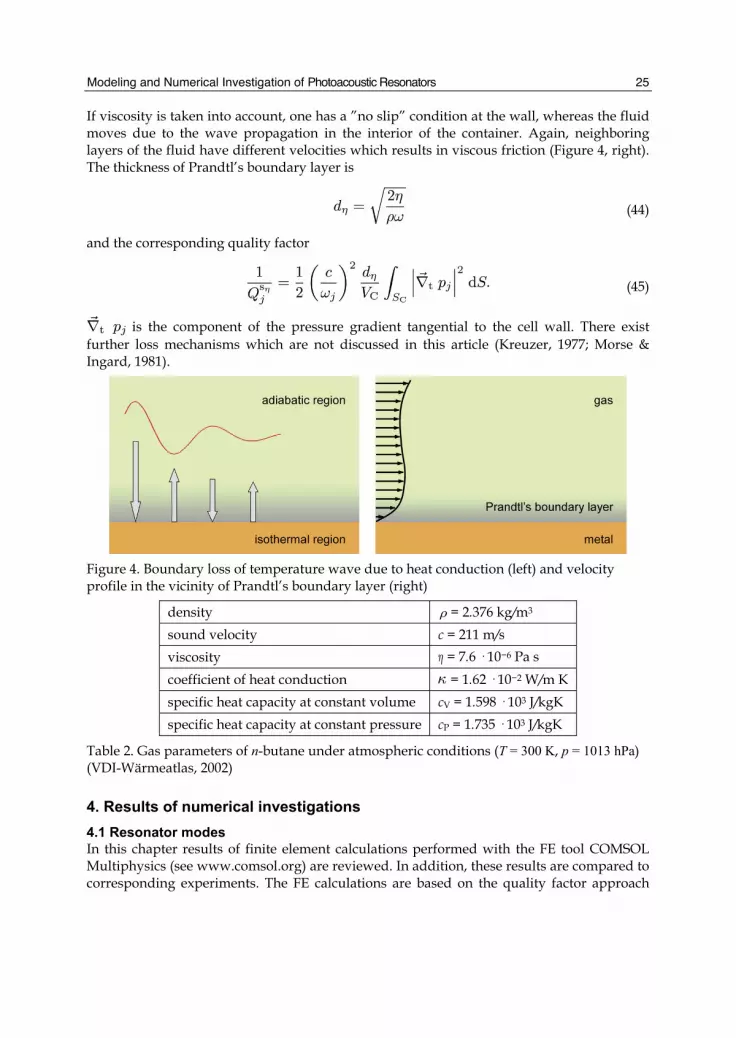
If viscosity is taken into account, one has a ”no slip” condition at the wall, whereas the fluid moves due to the wave propagation in the interior of the container. Again, neighboring layers of the fluid have different velocities which results in viscous friction (Figure 4, right). The thickness of Prandtl’s boundary layer is

(44)

and the corresponding quality factor

(45)

is the component of the pressure gradient tangential to the cell wall. There exist further loss mechanisms which are not discussed in this article (Kreuzer, 1977; Morse & Ingard, 1981).

Figure 4. Boundary loss of temperature wave due to heat conduction (left) and velocity profile in the vicinity of Prandtl’s boundary layer (right)

density = 2.376 kg/m3 sound velocity c = 211 m/s viscosity = 7.6 · 10−6 Pa s coefficient of heat conduction = 1.62 · 10−2 W/m K specific heat capacity at constant volume cV = 1.598 · 103 J/kgK specific heat capacity at constant pressure cP = 1.735 · 103 J/kgK

Table 2. Gas parameters of n-butane under atmospheric conditions (T = 300 K, p = 1013 hPa) (VDI-Wärmeatlas, 2002)

4. Results of numerical investigations 4.1 Resonator modes In this chapter results of finite element calculations performed with the FE tool COMSOL Multiphysics (see www.comsol.org) are reviewed. In addition, these results are compared to corresponding experiments. The FE calculations are based on the quality factor approach


26

described in Section 3.2. Since in this approach the acoustic pressure field inside the measuring chamber of the PA sensor is expressed as a sum over eigenmodes, a first and important step consists in the determination of the modes. Cylinder cells represent a perfect testing ground for the numerical analysis, because in this case the eigenfrequencies can be calculated analytically. Excellent agreement of analytical and numerical results has been found (Baumann et al., 2006). This confirms the reliability of the FE model used for the calculation of the modes of the T cell, where no analytical results are available. The physical parameters of n-butane used for the experiments and the simulations described in this article can be found in Table 2. In the following, we present results for T cells with different lengths LR of the resonance cylinder (see Table 3 and Figures 5 and 6). LR = 320 mm: All three lowest eigenmodes (1-3) are basically eigenmodes of the resonance

cylinder (one end open, one end closed), see Figure 5. This interpretation is confirmed by Table 3 and the observation that the acoustical pressure in the absorption cylinder is approximately zero (Figure 5, left). Only for the lowest eigenmode, a minor deviation from zero is observed. This and the deviation between finite element frequency and , the frequency of the half-open pipe, indicates, that the ground state (lowest eigenmode) is not a pure cylinder mode. The ground mode has been observed experimentally and the deviation between measured frequency and finite element result is small.

LR = 160 mm: The two lowest eigenmodes (1-2) are longitudinal modes of the resonance cylinder whereas the third mode is associated with the first longitudinal mode of the absorption cylinder (two closed ends). Because this mode shows a node at the opening of the resonance cylinder, it does not excite an oscillation in the resonance cylinder. Again, this interpretation is supported by Table 3 and the agreement between numerical result and measurement is excellent.

LR = 80 mm: The interpretation of the spectrum is essentially the same as in the case of the LR = 160 mm-T cell. Merely the order of the eigenmodes has changed: The first longitudinal mode of the absorption cylinder is now the second mode of the T cell. The agreement with the measured frequency is good.

LR = 40 mm: The ground state represents the first longitudinal mode of the resonance cylinder. The second mode is the first longitudinal mode of the absorption cylinder (see Figure 6). The length of the resonance cylinder now almost equals the length of the absorption cylinder. Therefore, the third mode shows an interesting characteristic: The second longitudinal mode of the absorption cylinder is excited. This mode shows an antinode at the opening of the resonance cylinder. Therefore, a

/2 –wave is excited in the resonance cylinder. That is, both the -wave of the absorption cylinder and the /2-wave in the half-open resonance cylinder are present. The latter would not be possible in the case of a single halfopen cylinder. The mode is depicted in Figure 7. Agreement with the measured frequency is good.

LR = 20 mm: Now, the first longitudinal mode of the absorption cylinder constitutes the ground state of the T cell. This mode cannot be detected experimentally due to the node at the opening of the resonance cylinder. The experiment detected the remnants of the resonance cylinder’s first longitudinal mode. The length of the resonance cylinder has now become similar to the diameter of resonance and absorption cylinder. Therefore, the formula of the half-open cylinder is not


27

applicable anymore. Figure 7 shows that the third mode cannot be disentangled into two cylinder modes.

LR = 10 mm: The ground state is again the first longitudinal mode of the absorption cylinder. The two higher modes cannot be brought into connection with cylinder modes. Both of these modes are detected experimentally.

For large lengths of the resonance cylinder one observes essentially modes, which are compatible with the well known formulae for the vibration of gas columns whereas for short resonance cylinders, this is no longer true. These observations are consistent with expectations and, therefore, we have a coherent picture of the T cell’s spectrum.

FEM Resonance Cyl. Absorption Cyl. Experiment

LR

[mm] Mode f [Hz]

f [Hz]

Dev. [%] Type f

[Hz] Dev. [%] Type f

[Hz] Dev. [%]

320 1 2 3

197.9 497.9 813.7

165.6 496.9 828.1

-16.3 -0.2 1.8

/4 3 /45 /4

203 2.6

160 1 2 3

354.0 953.2 1295.2

331.3 993.8

-6.4 4.3

/4 3 /4

1292.7

-0.2

/2

356 0.6

80 1 2 3

636.5 1295.21788.4

662.5 1987.5

4.1 11.1

/4 3 /4

1292.7

-0.2

/2

629 -1.2

40 1 2 3

1114.61295.22583.2

1325.0 2650.0

18.9 2.6

/4

/2

1292.72585.4

-0.2 0.1

/2

1092 -2.0

20 1 2 3

1295.21824.22684.3

1292.7 -0.2 /2 1722

-5.6

10 1 2 3

1295.22424.03124.0

1292.7 -0.2 /2 2392 3003

-1.3 -3.9

Table 3. Eigenfrequencies of the T cell for different lengths LR of resonance cylinder. The frequencies for resonance and absorption cylinder are calculated using the formula for gas columns. End corrections have not been included. The experimental frequencies are measured with an accuracy of about 1%. Due to the chosen frequency ranges not all of the numerically found eigenmodes have been measured


28

Absorption Cylinder Resonance Cylinder 32

0 m

m

160

mm

80 m

m

Figure 5. Pressure distribution of the three lowest nontrivial eigenmodes (1, 2, 3) of the T cell along the symmetry axis of the absorption cylinder and the resonance cylinder for LR = 320 mm , LR = 160 mm and LR = 80 mm. The actual length of the abscissa in the figures on the right-hand side is DA +LD +LR (see Table 1). The absolute values of the pressure is of no significance


29

Absorption Cylinder Resonance Cylinder 40

mm

20 m

m

10 m

m

Figure 6. Pressure distribution of the three lowest eigenmodes of the T cell for LR = 40 mm, LR = 20 mm and LR = 10 mm. For details consult the caption of Figure 5


30

Figure 7. Third mode of LR = 40 mm T cell (left) and of LR = 20 mm T cell (right). Depicted is |p|. For a proper interpretation consult Figure 6

4.2 Quality factors and amplitudes To calculate quality factors for PA resonators requires the evaluation of the surface integrals (43) and (45). If one even wants to calculate PA signals, in addition the volume integral (37) has to be calculated. Fortunately, for pure modes of low order of cylinder cells the surface integrals can be calculated analytically. Therefore, cylinder cells again have been used as a test case. Very good agreement of numerical results and exact formula has been observed (Baumann et al., 2007). We performed the calculations of the quality factors for T cells of various lengths of the resonance cylinder filled with n-butane and compared the results to measurement. For the numerical modeling of sound waves the characteristic FE size is required to be smaller than h = 0.2c/f, where c is the speed of sound and f the frequency of the sound wave. In our case the largest frequency of relevance is 3500 Hz. When calculating amplitudes, not only the sound waves but also the heat generating laser beam has to be resolved in the finite element mesh. Here, element sizes of h = 0.05c/f result in a satisfactory numerical accuracy. Modes of order higher than eight have no considerable contribution to the simulation. Therefore, we truncated the sum (33) after the 8th term. We have extracted resonance frequencies, quality factors and amplitudes by fitting Lorentzian profiles

(46)

to the experimental data. The quality factor is related to the half width (FWHM) of the resonance by . Two sets of data, together with the fit functions are exemplarily depicted in Figure 8. In Figure 9, values of the quality factors for resonance cylinders of length 1 cm to 14 cm are depicted. The obvious parallelism of the two curves demonstrates the suitability of the model for the description of sound propagation in photoacoustic measuring cells. For very short resonance cylinders only a deviation of the parallelism is observable. The fact, that experimental values are consistently smaller than FE values, is understandable because the


31

FE simulation does not include all effects that contribute to loss of the photoacoustic signal. For example, the microphone and its surrounding are not modeled in detail. The sharp edges and non-sound hard parts are not considered. Also, we did not model the gas inlet and gas outlet of the cell, which also add sharp edges. There might be impurities in the gas, that we do not have control of. Also, non negligible coupling of the sound wave with the gas container might occur. These and other origins of loss are not included in the FE model. Therefore, we expect higher loss, i. e. smaller quality factors, in the experiment than in the simulation. This is exactly what we observe. Furthermore, the amplitudes according to Equation (37) have been calculated. In order to evaluate the volume integral, we use the following description of the radiation intensity of the laser beam:

(47) We assume that the z-axis coincides with the symmetry axis of the absorption cylinder and

is the distance perpendicular to this axis (see Figure 10). w is the beam radius estimated to be 2 mm. The analytical calculation of the amplitudes according to Equation (37) with the Gaussian laser beam profile (47) is not even possible for the simple case of cylinder cells and numerical methods are necessary. Since we compare our FE results to the phase-sensitively amplified photoacoustic signals of T cells, absolute pressure values are not relevant. Therefore, the value of the product I0 can be used to rescale the numerical data. We performed a least square fit to adjust the parameter I0. Results are displayed in Figure 11. Numerical results and experimental results are in very good accordance. Once modes, quality factors and amplitudes are known, the PA signal can be calculated. Experimental and FE signals for a large variety of T cells are depicted in Figure 12. The good agreement is obvious. The experimental resonance amplitudes at low frequencies are smaller than the FE amplitudes. This could be attributed to the frequency characteristic of the microphone used for the measurements (Baumann et al., 2007).

4.3 Laser beam location for a T cell The sensitivity of a photoacoustic sensor depends on a variety of influences. Possible system variables of a photoacoustic cell could be e. g. geometrical dimensions, shape parameters, the location of the laser beam, the location of the resonance cylinder and the number and locations of microphones. In the following investigations as a measure of the signal strength of the photoacoustic cell the absolute value of the pressure field p at the microphone position will be used, i. e. the signal , where is the considered frequency range, can be calculated by a finite element analysis as described in Section 3. For the investigations described in this and in the following section the previously mentioned diminution has not been taken into account. Depending on how the laser beam is crossing the photoacoustic cell, different eigenmodes can be excited. The task is to find the beam position which leads to the strongest signal. The laser beam is assumed to be parallel to the z-axis (i. e. the axis of the absorption cylinder). For the investigation of the influence of the laser beam position the cross-sectional area has been covered by a regular grid (xi, yi) of evaluation points (see Figure 10 for the


32

coordinate system of a T cell). The grid points have to fulfill the inequaltity where is a given limit for the radius. This constraint has

been imposed to ensure a proper energy input into the system.

Figure 8. Experimental response function (dashed line) and corresponding fit (solid line) for the LR = 4 cm (upper) and LR = 8 cm (lower) T cell


33

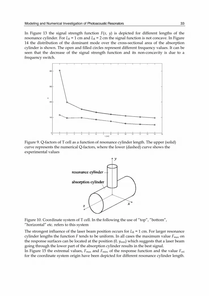
In Figure 13 the signal strength function F(x, y) is depicted for different lengths of the resonance cylinder. For LR = 1 cm and LR = 2 cm the signal function is not concave. In Figure 14 the distribution of the dominant mode over the cross-sectional area of the absorption cylinder is shown. The open and filled circles represent different frequency values. It can be seen that the decrease of the signal strength function and its non-concavity is due to a frequency switch.

Figure 9. Q-factors of T cell as a function of resonance cylinder length. The upper (solid) curve represents the numerical Q-factors, where the lower (dashed) curve shows the experimental values

Figure 10. Coordinate system of T cell. In the following the use of ”top”, ”bottom”, ”horizontal” etc. refers to this system

The strongest influence of the laser beam position occurs for LR = 1 cm. For larger resonance cylinder lengths the function F tends to be uniform. In all cases the maximum value Fmax on the response surfaces can be located at the position (0, ymin) which suggests that a laser beam going through the lower part of the absorption cylinder results in the best signal. In Figure 15 the extremal values, Fmax and Fmin, of the response function and the value Fori for the coordinate system origin have been depicted for different resonance cylinder length.


34

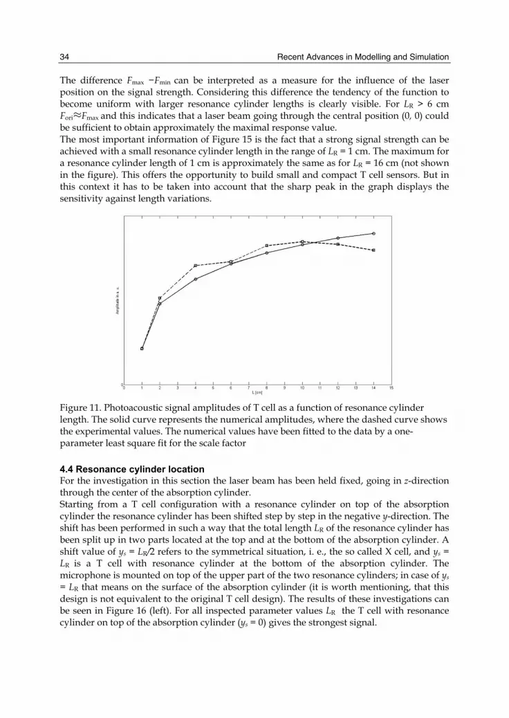
The difference Fmax −Fmin can be interpreted as a measure for the influence of the laser position on the signal strength. Considering this difference the tendency of the function to become uniform with larger resonance cylinder lengths is clearly visible. For LR > 6 cm Fori Fmax and this indicates that a laser beam going through the central position (0, 0) could be sufficient to obtain approximately the maximal response value. The most important information of Figure 15 is the fact that a strong signal strength can be achieved with a small resonance cylinder length in the range of LR = 1 cm. The maximum for a resonance cylinder length of 1 cm is approximately the same as for LR = 16 cm (not shown in the figure). This offers the opportunity to build small and compact T cell sensors. But in this context it has to be taken into account that the sharp peak in the graph displays the sensitivity against length variations.

Figure 11. Photoacoustic signal amplitudes of T cell as a function of resonance cylinder length. The solid curve represents the numerical amplitudes, where the dashed curve shows the experimental values. The numerical values have been fitted to the data by a one-parameter least square fit for the scale factor

4.4 Resonance cylinder location For the investigation in this section the laser beam has been held fixed, going in z-direction through the center of the absorption cylinder. Starting from a T cell configuration with a resonance cylinder on top of the absorption cylinder the resonance cylinder has been shifted step by step in the negative y-direction. The shift has been performed in such a way that the total length LR of the resonance cylinder has been split up in two parts located at the top and at the bottom of the absorption cylinder. A shift value of ys = LR/2 refers to the symmetrical situation, i. e., the so called X cell, and ys = LR is a T cell with resonance cylinder at the bottom of the absorption cylinder. The microphone is mounted on top of the upper part of the two resonance cylinders; in case of ys = LR that means on the surface of the absorption cylinder (it is worth mentioning, that this design is not equivalent to the original T cell design). The results of these investigations can be seen in Figure 16 (left). For all inspected parameter values LR the T cell with resonance cylinder on top of the absorption cylinder (ys = 0) gives the strongest signal.


35

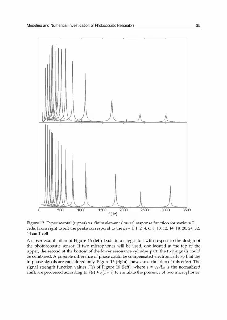
Figure 12. Experimental (upper) vs. finite element (lower) response function for various T cells. From right to left the peaks correspond to the LR = 1, 1, 2, 4, 6, 8, 10, 12, 14, 18, 20, 24, 32, 44 cm T cell

A closer examination of Figure 16 (left) leads to a suggestion with respect to the design of the photoacoustic sensor. If two microphones will be used, one located at the top of the upper, the second at the bottom of the lower resonance cylinder part, the two signals could be combined. A possible difference of phase could be compensated electronically so that the in-phase signals are considered only. Figure 16 (right) shows an estimation of this effect. The signal strength function values F(s) of Figure 16 (left), where s = ys /LR is the normalized shift, are processed according to F(s) + F(1 − s) to simulate the presence of two microphones.


36

The positions of the maxima in Figure 16 (right) show that the strongest signal can be achieved with asymmetrical cell types.

LR = 1 cm LR = 2 cm

LR = 4 cm LR = 8 cm

Figure 13. Signal strength function of T cells with different resonance cylinder length LR for the laser beam position problem

5. Conclusion We have performed the complete modeling of photoacoustic signal generation and detection using the finite element method. The model allows the calculation of photoacoustic response functions for any given cell geometry. Experimental and numerical results were found to be in good agreement. Furthermore the influence of certain design parameters on the signal has been investigated numerically. With respect to T cells the exploration shows that the laser position may have a strong effect depending on the length of the resonance cylinder. For short resonance cylinders strong signals can be achieved provided the laser beam is no longer centrally aligned. Additionally, it could be shown, that it might be useful to build asymmetrical photoacoustic cells with two microphones at the ends of the resonance cylinders.


37

LR = 1 cm LR = 2 cm

Figure 14. Distribution of dominating mode over the cross-sectional area of the absorption cylinder for the laser beam position problem for T cells with different resonance cylinder length LR. The open and filled circles represent different frequency values for each length LR

Figure 15. Comparison of extreme values of the signal strength function for a T cell with different resonance cylinder length LR


38

Figure 16. Signal strength function values for unconventionell cell shapes between T cell and X cell (left). Simulated signal of two combined microphones (right). The abszissa is s = ys/LR . s = 0 refers to a T cell with a resonance cylinder on top, s = 1 to a cell with a single resonance cylinder at the bottom of the absorption cylinder

6. References Baumann, B., Kost, B., Groninga, H. G. & Wolff, M. (2006) Eigenmode analysis of

photoacoustic sensors via finite element method, Review of Scientific Instruments, 77, 044901.

Baumann, B., Wolff, M., Kost, B. & Groninga, H. G. (2007) Finite Element Calculation of Photoacoustic Signals, Applied Optics, Vol. 46, No. 7, 1120-1125.

Bell, A. G. (1880) On the Production and Reproduction of Sound by Light, Am. J. Science 20, 305-309.

Haken, H. & Wolf, H. C. (1993) Molecular Physics and Quantum Chemistry, Springer- Verlag, Berlin.

Hess, ed. (1989) Photoacoustic, Photothermal and Photochemical Processes in Gases, Springer-Verlag, Berlin.

Kreuzer, L. B. (1977) The Physics of Signal Generation and Detection, in: Pao, Y.-H., ed., Optoacoustic Spectroscopy and Detection, Academic Press, New York, 1-25.

Miklós, A., Hess, P. & Bozóki, Z. (2001) Application of acoustic resonators in photoacoustic trace gas analysis and metrology, Rev. Sci. Instr., Vol. 2, No. 4, 1937-1955.

Morse, P. M. & Ingard, K. U. (1968) Theoretical Acoustics, McGraw-Hill, New York. Röntgen, W. C. (1881) Versuche über die Absorption von Strahlen durch Gase; nach einer

neuen Methode ausgeführt, XX. Bericht der Oberhessischen Gesellschaft für Natur- und Heilkunde, 52-58.

Temkin, S. (1981) Elements of Acoustics, JohnWiley & Sons, New York. VDI-Wärmeatlas (2002) 9. Auflage, Springer Verlag, Berlin. Wolff, M., Groninga, H. G., Baumann, B., Kost, B. & Harde, H. (2005) Resonance

Investigations using PAS and FEM, Acta Acustica, Vol. 91, Suppl. 1, 99. Zharov, V. P. & Letokhov, V. S. (1986) Laser Optoacoustic Spectroscopy, Springer Ser. Opt. Sci.

37, Springer Verlag, Berlin.

Documents

Modeling and Numerical Investigation of Photoacoustic Resonators