MODELING AND OPTIMIZATION OF WHEELED ROVERS

Pierre Lamon, Thomas Thüer, Rolf Jordi, Roland Siegwart

Autonomous Systems Laboratory

Swiss Federal Institute of Technology (EPFL), CH-1015 Lausanne {pierre.lamon, thomas.thueer, rolf.jordi, roland.siegwart }@epfl.ch

ABSTRACT

Due to the different properties of the dynamical simulation of multi-body systems, it is important to introduce a classifi-cation that allows for the right selection of a simulation type according to the user’s needs. The proposed classification divides simulations with respect to the main characteristics, such as speed, accuracy, processing power, preparation work, resulting in the need for very different models of the rover. Using the SOLERO rover as an example, problems are shown that can occur when developing a rover model, e.g. hy-per-statism. Applying simulation techniques, the rover geometry can be optimized regarding special metrics and the performance of different rovers can be compared. Experimental results of the implementation of a torque control algorithm underline the need and gain of the use of simulations in a development project.

Keywords - Wheeled rover, modeling, comparison, optimization, SOLERO, RCET

INTRODUCTION

Complexity of development projects, as well as pressure regarding time and costs have increased drastically in the past decades. In order to satisfy these demands it is crucial to use simulations in almost every stage of the project for the profound analysis of the new product and its components. There can be different kinds of simulations for the same application, which are used to assess different characteristics such as kinematics, dynamics, control or durability. Therefore the selection of the kind of simulation is very important and has to be done based on the requirements of the project. In the following sections a number of different approaches are presented, which are used to simulate dynamics of wheeled rovers with passive suspension structures. Apart from the results there are certain simulation characteristics that are of main interest, such as simulation speed, accuracy, processing power, preparation work, etc. According to these properties, rover simulations shall be classified into three main groups: 3D simulation using finite element method (FEM); full mathematical, mechanical model; constraint-based simulation. To emphasize the use and importance of rover simulation, a precise, optimized and verified, 3D-model of the 6-wheeled rover SOLERO [1] is presented which was used to develop a torque control algorithm to minimize slip and therefore increase terrainability.

SIMULATION CHARACTERIZATION

Wheeled rovers, in general, are complex mechanisms consisting of several bodies linked by different joints with vary-ing degrees of freedom (DoF). Such structures include closed kinematical loops, contain redundancy and are therefore subject to hyper-statism. Furthermore, the modeling of the wheel-soil interaction is quite complex. For all these reasons, the simulation of wheeled rovers is a very challenging task. In order to fulfill the project’s requirements it is necessary to make a trade-off when selecting the simulation type, be-cause there are different approaches to simulating articulated multi-body systems:

Type 1: 3D Simulation of CAD Models Using FEM

The 3D simulation with CAD (computer aided design) models is the industry standard. It is very precise thanks to the use of FEM calculations and even includes stress inside the components. Due to the character of FEM this simulation needs an enormous amount of processing power and thus, the simulation speed is very slow. Contrary to the widespread idea, 3D simulations need a lot of expert knowledge to be set up because inapt initial conditions can cause big errors in the results. The 3D simulation is suited only at later stages of the development when most of the design is known and CAD models are available. Therefore this simulation type serves rather for performance verification and optimization than for basic rover comparison. Example: SolidWorks model used in COSMOSMotion (ADAMS dynamics engine).

Type 2: Mechanical Model Based on Detailed, Mathematical Dynamics Equations

The high number of DoF of a rover results in a very complex mechanical rover model. Establishing the mathematical equations requires expert knowledge in mechanics of mechanisms including closed loops in order to avoid hyper-statism. All the equations for the balance of forces and moments have to be derived, which causes a lot of manual work and prevents easy adaptation of the model to new rover configurations. The complexity of the model is increasing su-perproportional when changing from a 2D to a 3D environment [2]. This approach is based on a quasi-static model, which is reasonable for rovers because of their low speed of only a few meters per hour. Since most of the work is done in advance, i.e. derivation of the complete model in a closed form, no iterations are necessary and therefore few processing power is required which increases simulation speed and makes the model suit-able for real-time applications. Example: SOLERO 3D model at EFPL implemented in SysQuake and C++.

Type 3: Generic Model Creation with Dynamics Based on Constraints

This is the only approach which allows for a generic model creation. The equations of motion don’t need to be derived, because the calculations are based on constraints (forces, joints) that the whole system must respect and the solution is found in an iterative, numerical process [4]. There are several libraries (dynamics engines) available (Open Dynamics Engine [5], Dynamechs [1], Vortex [7]) that can handle this kind of mathematical problem which is called Linear Con-straint Problem (LCP). The numerical iterations need computation power, but the simulations can still get close to real-time. The speed of the simulation can be decreased in order to increase the accuracy of the calculations. Not all information about the state of the mechanism is easily accessible.

Simulation Comparison

The following table shows a comparison of the different simulation types according to the characteristics, which were discussed above.

Table 1: Simulation type comparison Type 1 Type 2 Type 3 Simulation speed -- ++ + Processing power -- ++ + Accuracy ++ + +/- Manual work for model preparation (time)

- -- +

Prerequisites / required technical knowledge

- -- ++

(+ positive; +/- neutral; - negative)

MODEL AND OPTIMIZATION

At the Autonomous Systems Lab (ASL-EPFL) a lot of work has been conducted with simulation types 2 and 3 in the frame of different projects, like SOLERO and RCET [9]. The focus is laid on locomotion concepts because they are the basis for high terrainability of wheeled rovers. For the SOLERO rover (see Fig. 1A) a model has been developed that can be used for a simulation of type 2. This model is presented in the following sections and more details are available in [2].

Quasi-Static Model of a Wheeled Rover

Deriving the mechanical equations for the quasi-static model of a wheeled rover is a challenging task, especially when the rover contains parallel structures and closed kinematical loops because this can result in hyper-statism with more unknown variables than equations. For this reason it is important to analyze to mobility (MO) of the rover using Grubler’s Mobility Equation:

1 2 3 4 56 5 4 3 2MO n f f f f f= ⋅ − ⋅ − ⋅ − ⋅ − ⋅ − ( 1 )

where n is the number of bodies and fj the number of joints with the same number of DoF (j=1,..,5; for example f1 = number of pin joints; f3 = number of spherical joints). The mobility equation is a guideline for determining, if a system

is statically determinate. Many real systems contain redundancy in links and joints resulting in hyper-statism. Accord-ingly, using (1), the mobility for the SOLERO equals -20. In order to avoid the hyper-statism in the mechanical model the number of DoF is increased until the mobility of the system equals one, but of course the real behavior of the system must not change with the new number of DoF. A wheel-ground contact without slip can be modeled as a spherical joint with 3 DoF (rotations about the three axes). Since the lateral forces are not influenced by the wheel motor torque, an additional DoF was added to each wheel of the bogies of the SOLERO model. The remaining front and back wheels maintain their 3 DoF, not allowing lateral move-ment, and therefore the global behavior of the rover does not change. Similar changes to the model have been intro-duced at specific links on the bogies so that the mobility of the SOLERO model finally results in:

1627314145186 =⋅−⋅−⋅−⋅−⋅=MO ( 2 )

Fig. 1B shows the resulting kinematic model of the SOLERO rover. The numbers at the link connections indicate the DoF of that joint.

a) Steering servo mechanism b) Passively articulated bogie and spring suspended front fork (equipped with absolute angular sensors) c) One of the 6 motorized wheels d) Omnidirectional vision system e) Stereo-vision module f) Laptop. Not visible on the picture: an additional PC104 computer, electronics and an IMU (Inertial Measurement Unit)

Fig. 1: A) Sensors, actuators of SOLERO B) Mobility of the joints

Knowing the rover dimensions and the DoF of the rover, the balance of forces and moments (3 equations each) for every body can be worked out. Dynamical forces are considered to be negligible because the speed of such a rover is very low (~10 cm/s). Therefore, the model is referred to as quasi-static. Consisting of 18 bodies, the SOLERO model requires formulating 6*18 = 108 equations to describe the system’s static equilibrium. Taking into account the mobility of the joints, one can find 93 internal forces and torques, as well as 14 external forces resulting from the wheel ground contacts and 6 wheel torques. Since the internal forces are not of interest for the simulation, the system of equations can be simplified to 108 – 93 = 15 equations with the 20 unknowns remaining, which define 6 wheel torques and 14 wheel ground contacts forces. Finally, the model can be written as

1151202015 xxx RUM =⋅ ( 3 )

where M is the model matrix depending on the geometric parameters and the state of the robot, U a vector containing the unknown and R a constant vector. The solution space of such a system is of dimension 5: this means that there is an infinite set of solutions guaranteeing the equilibrium of the rover. However, it can be proved that the torques on the wheels are linearly dependent and that a set of equal torques is a solution of the system.

Structure Optimization

In a next step the structure of SOLERO was optimized, using the model and a parameter variation process to change the geometric dimensions of the structure and the position of the center of mass (CoM). The optimization was carried out

(A) (B)

on a step terrain taking the minimal friction coefficient (µ0 between the wheel and the soil) as well as the wheel torques that are needed to climb the step as optimization criteria [1]. The minimal friction coefficient guarantees that there is minimal slip and maximizes traction (drawbar pull), whereas minimal torques cause minimal energy consumption.

Comparison Between Different Rovers

Once the model has been optimized, it can be used for comparison with other rovers. To be able to compare wheeled rovers specific metrics have to be defined, which comply with the requirements of the project. Example for metrics: drawbar pull, ground clearance, minimal µ0, maximal wheel torque or energy consumption. Furthermore, the different rover models have to be normalized to specified outer dimensions (footprint) and weight. It is important for comparison that the rovers are similar; otherwise the simulation results have different meanings for dif-ferent rovers. More information about chassis comparison can be found in [9].

TORQUE CONTROL

An algorithm optimizing the control of the wheel motor torques in order to minimize wheel slip is presented in [2]. It uses the 3D pseudo-static model of SOLERO and accounts for physical constraints such as maximum available torques and positive reaction forces from the ground. Fig. 2 depicts the global optimization algorithm.

Fig. 2: Wheel torque optimization algorithm

However, its implementation on a real rover is not straightforward and more work has to be done. The following sec-tions propose concrete solutions and simulation results are presented.

Rover Motion

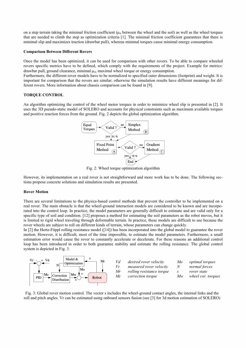
There are several limitations to the physics-based control methods that prevent the controller to be implemented on a real rover. The main obstacle is that the wheel-ground interaction models are considered to be known and are incorpo-rated into the control loop. In practice, the model parameters are generally difficult to estimate and are valid only for a specific type of soil and condition. [12] proposes a method for estimating the soil parameters as the robot moves, but it is limited to rigid wheel traveling through deformable terrain. In practice, these models are difficult to use because the rover wheels are subject to roll on different kinds of terrain, whose parameters can change quickly. In [2] the Hertz-Föppl rolling resistance model ([14]) has been incorporated into the global model to guarantee the rover motion. However, it is difficult, most of the time impossible, to estimate the model parameters. Furthermore, a small estimation error would cause the rover to constantly accelerate or decelerate. For these reasons an additional control loop has been introduced in order to both guarantee stability and estimate the rolling resistance. The global control system is depicted in Fig. 3.

Vd desired rover velocity Vr measured rover velocity Mr rolling resistance torque Mc correction torque

Mo optimal torques N normal forces s rover state Mw wheel cor. torques

Fig. 3: Global rover motion control. The vector s includes the wheel-ground contact angles, the internal links and the roll and pitch angles. Vr can be estimated using onboard sensors fusion (see [3] for 3d motion estimation of SOLERO)

The kernel of the control loop is a PID controller. It provides the additional torque to apply to the wheels in order to reach the desired velocity Vd. Mc is an estimate of the global rolling resistance torque Mr, which is considered as a perturbation by the PID controller. The rejection of the perturbation is guaranteed by the integral term of the PID. Be-cause the rolling resistance is proportional to the normal force, the individual corrections for the wheels are distributed using

ii

m

NMw McN

= ⋅

( 4 )

where Ni is the normal force on wheel i and Nm the average of all the normal forces. The derivative term of the PID allows accounting for non modeled dynamic effects and helps to stabilize the system. The parameters estimation for the controller is not critical because we are more interested in minimizing slip than in reaching the desired velocity in an optimal way. For locomotion in rough terrain, a residual error on the velocity can be accepted as long as slip is minimized. Furthermore, the system offers an intrinsic stability because the ratio between inertia and motor torques is large.

Experimental Results

A simulation phase has been initiated in order to test the algorithms and verify the theoretical concepts and assump-tions. The simulation parameters have been set as close as possible to the real operation conditions. However, the intent is not to get exact outputs but to compare different control strategies and detect/solve potential implementation prob-lems.

Simulation Tools

Simulations have been performed with the Open Dynamics Engine, which is a simulation tool of type 3. This engine is a platform independent and open source library for simulating rigid body dynamics in three dimensions. It has advanced joint types and integrated collision detection with friction. The source code being available it is possible to integrate more sophisticated simulation models such as rolling resistance, friction etc. In this application, a rolling resistance proportional to the normal force on the wheel has been implemented. This relation is generally assumed in the litera-ture. Table 2 presents a non-exhaustive list of the real rover parameters, which have been used in the simulation. All the geometric dimensions have been extracted from the mechanical drawings.

Table 2: SOLERO main characteristics

Rover body mass 7.4 kg Wheel mass 0.7 kg Steering mechanism mass 0.6 kg Spring constant 357 N/m Wheel diameter 0.15 m

The simulation tools allow to test and compare different traction control strategies. In these experiments, wheel slip has been taken as the main benchmark and the performance of torque and speed control have been compared. The imple-mented speed controller is the one presented in [10]. The slip of wheel i at time step k can be computed with:

( 1, ) ( 1, )i i ik k k k ks w Rθ− −= ∆ − ∆ ⋅

( 5 )

where ∆w is the true wheel displacement, ∆θ the angular change and R the wheel radius. The total slip of the rover occurring during an experiment is defined as

6

1

ik

i kS s

=

=∑∑

( 6 )

The body collision algorithm of ODE provides N contact points around the wheel together with the normal forces. This data is similar to what can be measured with a tactile wheel such as depicted in Fig. 4 (the tire compression is more or less proportional to the applied force).

Fig. 4 The tactile wheel (developed at EPFL by Michel Lauria) a) Sixteen infrared proximity sensors measure the tire compression all around the wheel. b) picture of an arm of the active robot Octopus equipped with tactile wheels [16].

The wheel-ground contact angles are computed with a weighted mean of the normal forces. In case the wheel does not touch the ground, the previously computed contact angle is taken.

Experiments

Two sets of experiments have been conducted. The first set comprises different terrain profiles in two dimensions (x and z) and the second, full 3D environments. In both cases, the nominal speed of the rover is 0.1 m/s and the friction coefficient has been set equal to 0.7.

Experiment Set Of Type One

Terrain profiles similar to the one depicted in Fig 5a have been generated and the simulation performed with both torque and speed control. Thanks to the terrain symmetry, the gravity center trajectories are the same whatever control type is used.

Fig. 5 a) Example of terrain of type one b) Total slip and rear wheel slip for both speed (spd) and torque (trq) control. Total slip is scaled by a factor of 500. Local wheel slip can be bigger with torque control but the total slip remains al-ways smaller.

Fig. 5b depicts typical results that have been obtained on such terrains. For a specific wheel, slip can be locally higher with torque control than with speed control. However, the total slip remains always smaller with torque control for all the experiments. Another interesting result is that the difference between the two methods increases when the friction coefficient gets lower. In other words, the advantage of using torque control becomes more and more interesting as the soil gets more slippery.

Experiment Set Of Type Two

Here, full three dimensional terrains are used for the experiments. They have been generated randomly with step, sinus, circle and particle deposition functions. This time, because the terrains are not symmetric, the trajectory of the rover depends on the control strategy. Therefore it is difficult to compare performance between torque and speed control.

b) a)

a) b)

However, we have considered an experiment as valid when the distance between the final positions of both trajectories is smaller than 0.1 m. This distance is small enough to allow performance comparison. For all the valid experiments, torque control showed better performance than speed control. In some cases the rover was even unable to climb some obstacles and to reach the final distance when driven with speed control. Otherwise, the simulations lead to the same conclusion as for the experiments of type one. Fig. 6a depicts one of the terrains used for the simulations and Fig. 6b the corresponding results.

Fig. 6 a) Snapshots of an experiment of type two. The total traveled distance along x is 3.5m. That kind of terrain is challenging for a wheeled rover because there is much side slip due to the fracture configuration. b) Total slip and front wheel slip for an experiment of type two. The difference gets bigger as the rover deals with true rough terrain. Total slip is scaled by a factor of 800.

Discussion

Strong assumptions have been used during the modeling phase i.e. no slip and the wheels touching the ground all the time. During simulation both assumptions have been violated but the system was able to recover and keep its stability, even in difficult situations such as depicted in Fig. 6a. Unless other control strategies, the proposed method does not include soil models. In a real application, the correspond-ing parameters are generally unknown because the rover is subject to deal with different types of soils, i.e. sand, rocks, gravel, grass and a combination of all of them. An error on the parameters estimation has a direct impact on the quality of the control. This can lead to bad performance and instability, which is critical during exploration missions. The simulations showed good results and promising perspectives. Furthermore, they allowed detecting potential prob-lems and addressing implementation details. This is a step closer to the real application. Moreover, the design of a me-tallic tactile wheel is currently investigated. Such a design will not only provide precious information such as wheel-ground contact angles but also allow more drawbar-pull, especially in sandy terrains. The simulations show clearly the advantage of torque control versus speed control. The algorithms can be run online and the first prototype of tactile wheel showed good results. Thus, the success probability during the implementation phase on a real rover can be considered as high.

CONCLUSION

Due to the different properties of dynamical simulations of multi-body systems a classification has been introduced that takes into account the main characteristics of simulations such as simulation speed, accuracy, processing power, prepa-ration work. Three groups result from these criteria: 3D simulation using finite element method (FEM); full mathemati-cal, mechanical model; constraint-based simulation. Furthermore, a quasi-static rover model of simulation type 2 was presented including the discussion of the system’s DoF and how to solve problems concerning hyper-statism. In a parameter variation process the geometrical structure was optimized by minimizing the needed friction coefficient (µ0) to overcome the test obstacle (step) and therefore minimize slip.

b) a)

In order to compare rovers equal conditions have to be given. This means that special metrics have to be defined and the rovers have to be normalized to have the same footprint and weight. In the second part of the paper the implementation of a torque control algorithm is described to underline the need and use of simulations. The experimental results clearly show that the torque control minimizes slip better than speed con-trol. Even though local maximum values can be bigger, the total slip is reduced significantly. With the help of simula-tions implementation problems can be uncovered and solved in an early stage of the project, speeding up the whole development.

REFERENCES

[1] Michaud S., Schneider A., Bertrand R., Lamon P., Siegwart R., et al., “SOLERO: Solar-powered exploration rover“, Proceedings of the 7th ESA Workshop on Advanced Space Technologies for Robotics and Automation, The Netherlands, ASTRA2002, 2002.

[2] Lamon P., Krebs A., Lauria M., Shooter S. and Siegwart R., "Wheel torque control for a rough terrain rover", IEEE International Conference on Robotics and Automation, New Orleans, USA, 2004.

[3] Lamon P., Siegwart R., "Inertial and 3D-odometry fusion in rough terrain – Towards real 3D navigation", IEEE/RSJ International Conference on Intelligent Robots and Systems, Sendai, Japan, 2004.

[4] Baraff D. and Witkin A., “Physically Based Modeling: Principles and Practice”, Online Siggraph '97 Course notes, Carnegie Mellon University, 1997.

[5] Open Dynamics Engine: http://www.ode.org. [6] Dynamechs: http://dynamechs.sourceforge.net. [7] Vortex by CM-Labs: http://www.cm-labs.com. [8] Siegwart R., Lamon P., Estier T., Lauria M., Piguet R., "Innovative design for wheeled locomotion in rough

terrain", Journal of Robotics and Autonomous Systems, Elsevier, vol 40/2-3 p151-162. [9] Michaud S., Patel N., Siegwart R., Richter L., Ellery A., “RCET: Rover Chassis Evaluation Tool”, Proceedings

of the 8th ESA Workshop on Advanced Space Technologies for Robotics and Automation, The Netherlands, ASTRA2004, 2004.

[10] Baumgartner E. T., Aghazarian H., Trebi-Ollennu A., Huntsberger T. L., Garrett M. S., "State Estimation and Vehicle Localization for the FIDO Rover", Sensor Fusion and Decentralized Control in Autonomous Robotic Systems III, SPIE Proc. Vol. 4196, Boston, USA, 2000.

[11] Iagnemma K. and Dubowsky S., Mobile Robot Rough-Terrain Control (RTC) for Planetary Exploration”, Pro-ceedings of the 26th ASME Biennal Mechanisms and Robotics Conference, DETC 2000, 2000.

[12] Iagnemma K., Shibley H., Dubowsky S., "On-Line Terrain Parameter Estimation for Planetary Rovers", IEEE International Conference on Robotics and Automation, Washington D.C, USA, 2002.

[13] Iagnemma K., Dubowsky S., “Vehicle Wheel-Ground Contact Angle Estimation: with application to Mobile Robot Traction Control”, 7th International Symposium on Advances in Robot Kinematics, ARK ‘00, 2000.

[14] Kalker J.J., "Three dimensional elastic bodies in rolling contact", Kluwer Academic Publishers, Dordrecht, 1990. [15] Weisbin, C., Rodriguez, G., Schenker, P., Das, H.,Hayati, S., Baumgartner, E., Maimone, M., Nesnas,I., and

Volpe, R., “Autonomous Rover Technologyfor Mars Sample Return”, 1999 InternationalSymposium on Artifi-cial Intelligence, Robotics andAutomation in Space (i-SAIRAS ‘99), 1999.

[16] Lauria M., Piguet Y. and Siegwart R., "Octopus - An Autonomous Wheeled Climbing Robot", In Proceedings of the Fifth International Conference on Climbing and Walking Robots, Published by Professional Engineering Publishing Limited, Bury St Edmunds and London, UK, 2002.