This content has been downloaded from IOPscience. Please scroll down to see the full text.

Download details:

This content was downloaded by: levineh

IP Address: 128.42.166.202

This content was downloaded on 01/12/2013 at 12:39

Please note that terms and conditions apply.

Modeling cell-death patterning during biofilm formation

View the table of contents for this issue, or go to the journal homepage for more

2013 Phys. Biol. 10 066006

(http://iopscience.iop.org/1478-3975/10/6/066006)

Home Search Collections Journals About Contact us My IOPscience

IOP PUBLISHING PHYSICAL BIOLOGY

Phys. Biol. 10 (2013) 066006 (8pp) doi:10.1088/1478-3975/10/6/066006

Modeling cell-death patterning duringbiofilm formationPushpita Ghosh1, Eshel Ben-Jacob1,2 and Herbert Levine1,3

1 Center for Theoretical Biological Physics, Rice University, Houston, TX 77005, USA2 School of Physics and Astronomy, Tel Aviv University, Tel Aviv 69978, Israel3 Department of Bioengineering, Rice University, Houston, TX 77005, USA

E-mail: herbert.levine@rice.edu

Received 13 August 2013Accepted for publication 1 November 2013Published 26 November 2013Online at stacks.iop.org/PhysBio/10/066006

AbstractSelf-organization by bacterial cells often leads to the formation of a highly complexspatially-structured biofilm. In such a bacterial biofilm, cells adhere to each other and areembedded in a self-produced extracellular matrix (ECM). Bacillus substilis bacteria utilizelocalized cell-death patterns which focuses mechanical forces to form wrinkled sheet-likestructures in three dimensions. A most intriguing feature underlying this biofilm formation isthat vertical buckling and ridge location is biased to occur in region of high cell-death. Herewe present a spatially extended model to investigate the role of the bacterial secreted ECMduring the biofilm formation and the self-organization of cell-death. Using thisreaction-diffusion model we show that the interaction between the cell’s motion and the ECMconcentration gives rise to a self-trapping instability, leading to variety of cell-death patterns.The resultant spot patterns generated by our model are shown to be in semi-quantitativeagreement with recent experimental observation.

1. Introduction

Microbial cells often self-organize in a collective manneron a solid surface or on a liquid–air interface, forming astructurally complex multicellular community known as abiofilm [1–3]. Biofilm formation is a nearly universal bacterialtrait and therefore biofilms are widespread in nature [4–7].They are responsible for many serious problems in medical[8, 9] and industrial [10] contexts but sometimes can alsobe beneficial, for example, in waste-water treatment, plantprotection, and as potential source of energy in the formof microbial fuel cells [11–13]. The characteristic featureof any biofilm is that the cells are embedded in a self-produced extracellular matrix (ECM) [14–17]. ECM mainlyconsists of molecules of polysaccharides, proteins and nucleicacids but the exact composition depends on the strain of thebacterium and the type of nutrients present in the culturemedium [15]. ECM provides microbial cells a hydratedenvironment, and gives structural and mechanical stability tothe biofilm. Biofilm development is influenced by a numberof different processes, including the genetically controlledcell growth/death and differentiation, and the macroscopic

movements of the cell-population as determined by physicalforces. In response to varying environmental conditions,the film can adopt different structural phenotypes rangingfrom homogeneous mono-layers, to heterogeneous three-dimensional structures including mushrooms and filaments[18], with elastic properties allowing them to display ripplingand streaming [19–22]. Sometimes, biofilms exhibit rich three-dimensional spatial structures in the forms of wrinkles andfolds.

Biological pattern formation is ubiquitous and thesepatterns often play vital roles in embryogenesis anddevelopment [23, 24]. Pattern formation in bacterial systemshas been a major area of research for the last several decades[25–31]. In many of these cases bacteria undergo patternformation due to their chemotactic response [32–34]. Recently,it has been theoretically proposed that density suppressingmotility could also lead to patterns via a ‘self-trapping’mechanism [35–38]. In this respect it has been shown thatE. coli in which motility has been made density dependentby artificially coupling it to quorum sensing signals, generateperiodic stripes of high and low density when spotted on agarplates [39, 40].

1478-3975/13/066006+08$33.00 1 © 2013 IOP Publishing Ltd Printed in the UK & the USA

Phys. Biol. 10 (2013) 066006 P Ghosh et al

Here we focus on the spatiotemporal dynamics ofBacillus, which has long served as a model for the studyof biofilm formation [41–46]. Recently, it has been shownthat under certain conditions Bacillus substilis cells formwrinkled biofilms [43] in three-dimensions. The most strikingfeature behind this wrinkle formation is its connection tolocalized cell-death which apparently can serve to spatiallyfocus mechanical forces and thereby causes vertical bucklingwhich leads to wrinkle formation. Cell-death patterning occursprior to the wrinkle formation and hence acts as a mechanical‘pre-pattern’. A theoretical model was proposed in [43] todescribe the observed cell-death patterns but the model is basedmainly on the assumption of heterogeneous growth rate. In thispaper, we investigate the interplay between Bacillus subtiliscells and the self-produced ECM, and show that this interactionleads naturally to the aforementioned self-trapping type ofinstability. Thus instability then leads to a heterogeneous cell-death pattern.

2. Model

2.1. A reaction-diffusion-drift model

To account for the phenomena of heterogeneous cell-deathduring the formation of wrinkled biofilms in Bacillus substilis,we focus on the coupled spatiotemporal dynamics of bacterialcells and ECM. This ECM basically consists of polysacharidesand amyloid fibers which are produced by the bacterial cells.In our model, we assume the ECM when initially extrudedstarts out having a very low diffusivity compared to bacterialcells; our model does not include ECM mechanical effectsonce it gels into a solid matrix. The presence of the ECMcomponents traps the cells and hence precludes the bacterialcells traveling from higher density region to lower densityregions.

There are different possible ways in which bacteria canmove. In suspensions, or on moist agar surfaces, cells canpropel themselves forward by rotating their flagella. Insidedense aggregates of the type more typical of the biofilmcontext, it is more likely that the cells would employ pili-based twitching motion [35]. It is even conceivable that insome instances the bacteria are no longer able to move inan active manner and cell translocation occurs as a passiveresponse to growth. As pointed out by Cates and co-workers[36, 37], the statistical mechanics of the active particles [38] isvery different than what we expect for typical Brownian motionwith respect to how particles (modeled cells or agents here)respond to gradients in their motility. In particular, equilibriumsystems respond to gradients in the motility caused for exampleby viscosity gradients by a purely diffusive-type flux:

j = −D(x)∂ρ

∂x

where ρ is the density of bacterial cells. This guarantees thatthe system has the proper equilibrium distribution. But thisis no longer the case when the motion is active. This wasworked out in detail for the type of run-and-tumble dynamicstypical of flagellum-mediated motion. On a macroscopic scale

for a uniform system the motion of individual bacteria ischaracterized by a diffusivity of D = ν2τ/(ND), where ν

is the local run speed, τ the time between tumbles and ND thedimensionality. The crucial feature is that a nonuniform swimspeed ν(x) can cause a mean-drift velocity in the diffusivelimit. Following [34], one can derive the total flux of thebacterial cells in one dimension as

j = −ν(x)2τ (x)∂ρ

∂x− ν(x)τ (x)ρ

∂ν(x)

∂x.

The term proportional to ∇ρ represents the flux contributionfrom purely random diffusive motion, while the termproportional to ρ is a novel flux contribution proportional toan effective drift velocity V = −ντ∇ν. The negative signimplies that particles tend to drift toward regions where thespeed is low. If the speed is a decreasing function of density,this term can lead to macroscopic phase separation betweenregions of high bacterial density, where particles are trapped,and co-existing regions of low density.

It is critical to point out that the velocity trappingphenomenon does not depend on the motion being driven bythe flagellum, but is expected by general principles to be afeature of any spatially-varying self-propulsion mechanism.Here we will focus on the fact that motility is suppressed byECM concentration E. This translates into a dependence ofthe speed on E(x), which via the aforementioned mechanismbecomes a term in the bacterial flux of the form of an effectivedrift

−→V (E ) = −D′(E )∇E. (1)

Hence the total flux of the bacterial cells becomes

j = −D(E )∇ρ + ρ−→V (E ). (2)

As E will ultimately be secreted by the cells and hencebe correlated with cell density, this model can exhibit self-trapping. Our notion here is similar to the artificial quorum-sensing-mediated effect in [39, 40], except that it occursnaturally in biofilms and that the detailed dependence on theECM concentration is likely to be very different.

The rest of our model is as follows. We use a standardreaction-diffusion framework to describe the birth, death andmotility of the bacteria. This is then coupled to the ECMdynamics, giving us the schematic spatiotemporal system:

∂ρ(x, t)

∂t= Birth–death + Density dependent dispersal, (3)

∂E(x, t)

∂t= ECM production–degradation + Diffusion. (4)

To this end we are considering the simple model ofpopulation dynamics in a nutrient-rich medium based onbirth and death processes which is accounted through alogistic growth term of the form αρ(1 − ρ/ρ0). Thisexpression describes a population that evolves, from aboveor below towards a target density ρo which depends on theenvironmental conditions. The parameter α represents thegrowth rate of bacterial cells. The ECM concentration isalso a dynamic variable which undergoes changes due to itsproduction and degradation and its dispersion through space.

2

Phys. Biol. 10 (2013) 066006 P Ghosh et al

We employ a bi-continuum approach and ignore the precisegeometry of the ECM as well as its mechanical properties.As ECM molecules are secreted from cells we can write theproduction term following a Hill-kinetics which is a functionof bacterial cell density,

μ

⎡⎣

(ρ

ρk

)n

1 +(

ρ

ρk

)n

⎤⎦ ,

and a linear decay term (βE) which arises due to thedegradation of ECM. Here, the parameters μ and β representthe (asymptotic) ECM production rate and degradation raterespectively. The parameter ρk differs in general from thesaturation density of bacterial population ρo and governs theproduction term. The full dynamics are given by:

∂ρ

∂t= αρ(1 − ρ/ρ0) + ∇.[(D(E )∇ρ) − ρ

−→V (E )] (5)

∂E

∂t= μ

⎡⎣

(ρ

ρk

)n

1 +(

ρ

ρk

)n

⎤⎦ − βE + dE∇2E (6)

where the diffusion coefficient of bacterial cell is presumedto be an exponential decaying function of ECM density:D(E ) = Doe−pE where Do is the free diffusion coefficient ofbacterial cell and where p is a parameter having the dimensionof inverse of concentration, and dE is the diffusivity of ECM.

To ease comparison with experimental observations, timeis measured in hours and length is measured in micrometer.Correspondingly, bacterial density is measured in units of(cell number) (μm−2), bacteria growth rate (α) is measuredin units of 1 (h)−1 and the diffusion coefficient is measured inunits of (μ2)/(h)−1. ECM is represented in units of bacterialdensity, hence the degradation rate parameter (γ ) is measuredin units of 1/(h)−1 and the ECM production rate parameter(σ )is measured in units of (cell number) (μ−2) (h−1).

To rewrite the model in a dimensionless form we rescalethe variables and parameters such that the equations now readas

∂u

∂t ′= f (u) + ∇.[D(w)(∇u − u∇w)] (7)

∂w

∂t ′= g(u, w) + d∇2w (8)

where the dimensionless quantities are expressed as: ρ/ρo =u, ρk/ρo = uk, pE = w, αt = t ′, σ = pμ/α, γ = β/α,d = dE/Do and (α/Do)

1/2r = r̃. Here the functions f , g andD have the following form:

f (u) = u(1 − u) (9)

g(u, w) = σ

⎡⎣

(uuk

)n

1 +(

uuk

)n

⎤⎦ − γw (10)

D(w) = e−w. (11)

For convenience, the variables and parameters contributing forthe spatiotemporal dynamics are listed in table 1.

The homogeneous steady states of the dynamical systemare the fixed points us and ws defined by f (us) =0, g(us, ws) = 0 which are obtained as

Table 1. The dimensionless variables and parameters

Dimensionlessvariables/parameters Form Description

u ρ/ρo Bacterial cell densityw pE ECM densityσ pμ/α Production rate of ECMγ β/α Degradation rate of ECMuk ρk/ρo Density-threshold for ECM

productiond dE/Do Ratio of diffusion coefficientsn A number Hill-coefficient

(i) us = 0, ws = 0 and

(ii) us = 1, ws = σ

γ

⎡⎣

(usuk

)n

1 +(

usuk

)n

⎤⎦ . (12)

To test how the system responds when it is perturbed aroundthe homogeneous steady state (us, ws), we have carriedout a linear stability analysis. The details of the stabilityanalysis is described in the appendix. The system exhibitsa symmetry-breaking spatial instability; the necessary andsufficient condition for spatial instability is described byequation (A.15). The bifurcation curve is obtained as follows

− d +[

nσ (1/uk)n

(1 + (1/uk)n)2− γ

]e−ws = 2

√γ d e−ws . (13)

2.2. Numerical simulations: phase-field method

We have utilized the phase-field method [47] to numericallysolve the original system equations (7) and (8). We chose thisapproach to facilitate the numerical simulations in a circulargeometry, handling the zero-flux boundary condition correctly;in the limit of the phase field having a sharp transition zone,the equations reduce exactly to the usual formulation. Thismethod has traditionally been used to solve a number offree-boundary problems such as dendritic solidification [48],viscous figuring [49], crack propagation [50, 51] and canalso be applied to diffusional problems having stationary butcomplicated geometry. The basic idea involves distinguishingbetween the spatiotemporal dynamics of the system insidethe circular area apart from the outside. This can be obtainedmultiplying a phase-field variable with the actual dynamicalequations and then extending them to all of space. As a phase-field we have chosen a function φ(r) that has the explicitform as

φ(r) = 12 + 1

2 tanh[(r0 − r)/ξ ], (14)

where the phase field has the value +1 inside the circulardomain specified by a radius r0, 0 outside and varies betweenthese two values across a diffusive boundary layer of thicknessξ . One can show that in the limit of ξ → 0 the appropriateboundary conditions are recovered [47]. In our case the modelbecomes∂(φρ)

∂t= φαρ(1 − ρ/ρ0) + ∇.φ[(D(E )∇ρ) − ρ

−→V (E )],

(15)

3

Phys. Biol. 10 (2013) 066006 P Ghosh et al

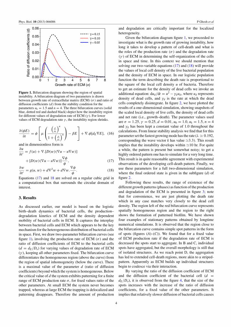
Figure 1. Bifurcation diagram showing the region of spatialinstability. A bifurcation diagram of two parameters is drawnbetween growth rate of extracellular matrix (ECM) (σ ) and ratio ofdiffusion coefficients (d) from the stability condition for theparameters uk = 1.5 and n = 4. The three bifurcation curves (solidblue, dotted red and dashed black) depict how the instability regionfor different values of degradation rate of ECM (γ ). For lowervalues of ECM degradation rate γ , the instability region shrinks.

∂(φE )

∂t= φ

⎡⎣μ

⎛⎝

(ρ

ρk

)n

1 +(

ρ

ρk

)n

⎞⎠ − βE

⎤⎦ + ∇.φ[dE∇E], (16)

and in dimensionless form is∂u

∂t ′= f (u) + ∇.[D(w)(∇u − u∇w)]

+ [D(w)(∇u − u∇w)]∇φ

φ, (17)

∂w

∂t ′= g(u, w) + d∇2w + d∇w.

∇φ

φ. (18)

Equations (17) and 18 are solved on a regular cubic grid ina computational box that surrounds the circular domain ofinterest.

3. Results

As discussed earlier, our model is based on the logisticbirth–death dynamics of bacterial cells, the production–degradation kinetics of ECM and the density dependentmobility of bacterial cells in ECM. It captures the interplaybetween bacterial cells and ECM which appears to be the keymechanism for the heterogeneous distribution of bacterial cellsin space. First, we draw two-parameter bifurcation curves (seefigure 1), involving the production rate of ECM (σ ) and theratio of diffusion coefficients of ECM to the bacterial cells(d = dE/Do) for varying values of degradation rate of ECM(γ ), keeping all other parameters fixed. The bifurcation curvedifferentiates the homogeneous region (above the curve) fromthe region of spatial inhomogeneity (below the curve). Thereis a maximal value of the parameter d (ratio of diffusioncoefficients) beyond which the system is homogeneous. Belowthe critical value of d the system exhibits patterning for a finiterange of ECM production rate σ , for fixed values ratio of theother parameters. At small ECM the system never becomestrapped, whereas at large ECM the trapping is delocalized andpatterning disappears. Therefore the amount of production

and degradation are critically important for the localizedheterogeneity.

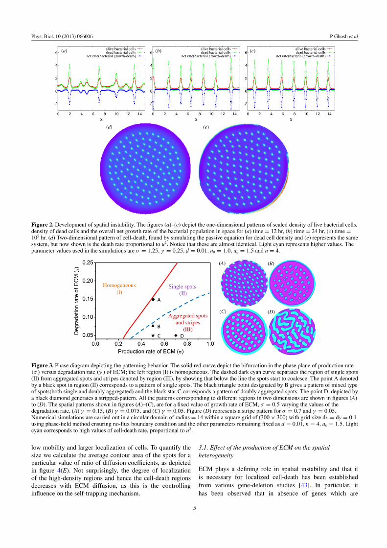
Given the bifurcation diagram figure 1, we proceeded toinvestigate what is the growth rate of growing instability, howlong it takes to develop a pattern of cell-death and what isthe roles of the production rate (σ ) and the degradation rate(γ ) of ECM in determining the self-organization of the cellsin space and time. In this context we should mention thatsolving our two-variable equations (17) and (18) will providethe values of local cell density of the live bacterial populationand the density of ECM in space. In our logistic populationfunction the term describing the death rate is proportional tothe square of the local cell density u of bacteria. Thereforeto get an estimate for the density of dead cells we invoke anadditional equation: dud/dt = u2 − γdud , where ud representsdensity of dead cells, and γd is the rate at which the deadcells completely disintegrate. In figure 2, we have plotted theresults of a one-dimensional simulation, showing snapshots ofthe scaled local density of live cells, the density of dead cellsand net rate (i.e., growth–death). The parameter values usedare σ = 1.25, γ = 0.25, d = 0.01, u0 = 1.0, uk = 1.5, n = 4and γd has been kept a constant value of 1.0 throughout thecalculations. From linear stability analysis we find that for thisparameter set the fastest growing mode has the rate (λ � 0.192,corresponding the wave vector k has value �3.3). This resultimplies that the instability develops within �10 hr. For quitea while, the pattern is present but somewhat noisy; to get ahighly ordered pattern one has to simulate for a very long time.This result is in quite reasonable agreement with experimentalobservations of the developing cell-death pattern. Finally, weuse these parameters for a full two-dimensional simulation,where the final ordered state is given in the subfigure (d) offigure 2.

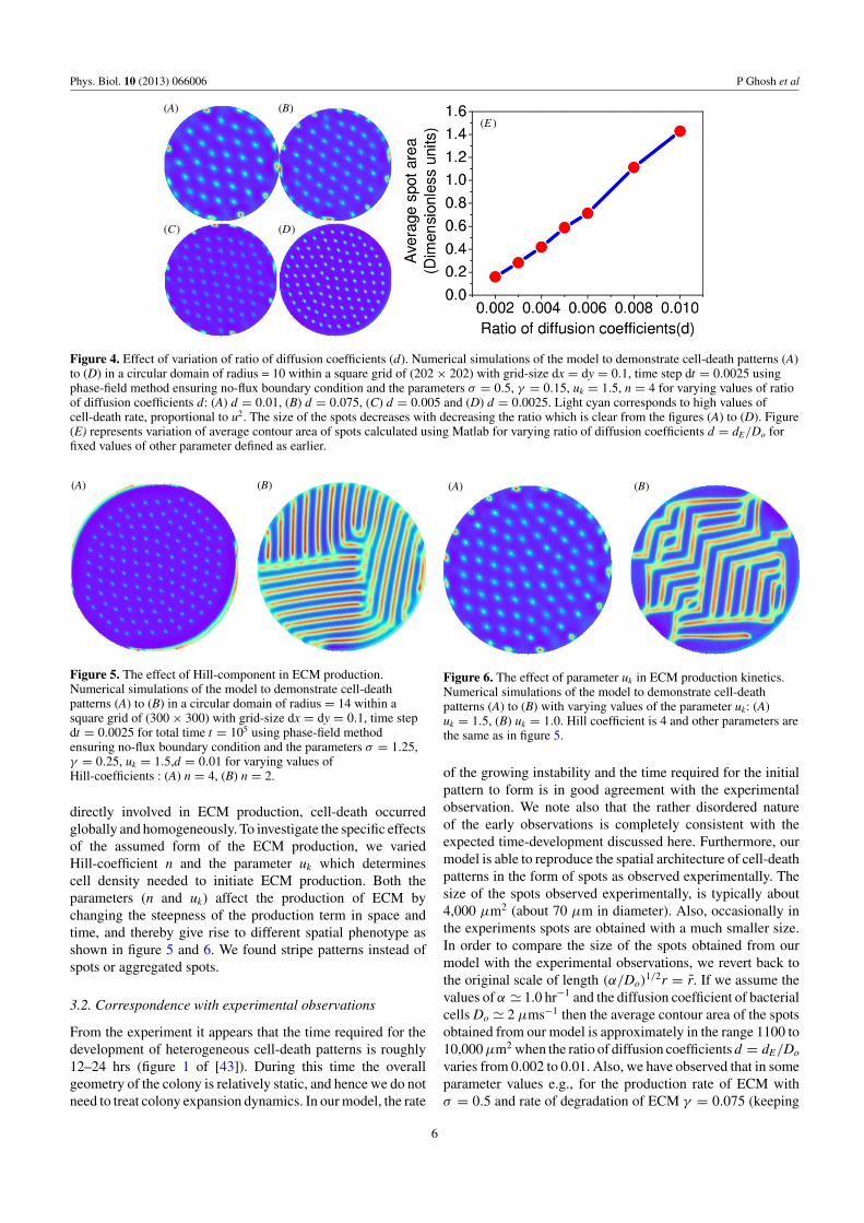
Following these results, the range of existence of thedifferent growth patterns (phases) as function of the productionand degradation of the ECM is presented in figure 3; notethat for convenience, we are just plotting the death ratewhich in any case matches very closely to the dead celldensity. The region left of the red bifurcation curve representsspatially homogeneous region and the region to the rightshows the formation of patterned biofilm. We have shownfour examples of stationary patterns obtained by longtimenumerical simulations. It is observed that the region close tothe bifurcation curve contains simple spot patterns in the formof spots (figures (A)–(C)). We found that for a fixed valueof ECM production rate if the degradation rate of ECM isdecreased the spots start to aggregate. In B and C, individualspots have aggregated, but the overall morphology is still thatof isolated structures. As we reach point D, the aggregationhas led to extended cell-death regions, more akin to a striped-pattern. Apparently as ECM builds up individual structuresbegin to coalesce via their interaction.

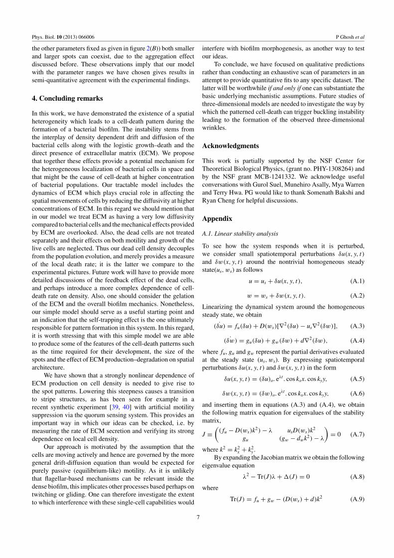
By varying the ratio of the diffusion coefficient of ECMand the diffusion coefficient of the bacterial cell (d =dE/Do), it is observed from the figure 4, that the size of thespots increases with the increase of the ratio of diffusioncoefficients, for a fixed value of the other parameters. Itimplies that relatively slower diffusion of bacterial cells causes

4

Phys. Biol. 10 (2013) 066006 P Ghosh et al

(a) (b) (c)

(d) (e)

Figure 2. Development of spatial instability. The figures (a)–(c) depict the one-dimensional patterns of scaled density of live bacterial cells,density of dead cells and the overall net growth rate of the bacterial population in space for (a) time = 12 hr, (b) time = 24 hr, (c) time =105 hr. (d) Two-dimensional pattern of cell-death, found by simulating the passive equation for dead cell density and (e) represents the samesystem, but now shown is the death rate proportional to u2. Notice that these are almost identical. Light cyan represents higher values. Theparameter values used in the simulations are σ = 1.25, γ = 0.25, d = 0.01, u0 = 1.0, uk = 1.5 and n = 4.

(A)

(C) (D)

(B)

Figure 3. Phase diagram depicting the patterning behavior. The solid red curve depict the bifurcation in the phase plane of production rate(σ ) versus degradation rate (γ ) of ECM; the left region (I) is homogeneous. The dashed dark cyan curve separates the region of single spots(II) from aggregated spots and stripes denoted by region (III), by showing that below the line the spots start to coalesce. The point A denotedby a black spot in region (II) corresponds to a pattern of single spots. The black triangle point designated by B gives a pattern of mixed typeof spots(both single and doubly aggregated) and the black star C corresponds a pattern of doubly aggregated spots. The point D, depicted bya black diamond generates a stripped-pattern. All the patterns corresponding to different regions in two dimensions are shown in figures (A)to (D). The spatial patterns shown in figures (A)–(C), are for a fixed value of growth rate of ECM, σ = 0.5 varying the values of thedegradation rate, (A) γ = 0.15, (B) γ = 0.075, and (C) γ = 0.05. Figure (D) represents a stripe pattern for σ = 0.7 and γ = 0.05.Numerical simulations are carried out in a circular domain of radius = 14 within a square grid of (300 × 300) with grid-size dx = dy = 0.1using phase-field method ensuring no-flux boundary condition and the other parameters remaining fixed as d = 0.01, n = 4, uk = 1.5. Lightcyan corresponds to high values of cell-death rate, proportional to u2.

low mobility and larger localization of cells. To quantify thesize we calculate the average contour area of the spots for aparticular value of ratio of diffusion coefficients, as depictedin figure 4(E). Not surprisingly, the degree of localizationof the high-density regions and hence the cell-death regionsdecreases with ECM diffusion, as this is the controllinginfluence on the self-trapping mechanism.

3.1. Effect of the production of ECM on the spatialheterogeneity

ECM plays a defining role in spatial instability and that itis necessary for localized cell-death has been establishedfrom various gene-deletion studies [43]. In particular, ithas been observed that in absence of genes which are

5

Phys. Biol. 10 (2013) 066006 P Ghosh et al

(A) (B)(E )

(C) (D)

Figure 4. Effect of variation of ratio of diffusion coefficients (d). Numerical simulations of the model to demonstrate cell-death patterns (A)to (D) in a circular domain of radius = 10 within a square grid of (202 × 202) with grid-size dx = dy = 0.1, time step dt = 0.0025 usingphase-field method ensuring no-flux boundary condition and the parameters σ = 0.5, γ = 0.15, uk = 1.5, n = 4 for varying values of ratioof diffusion coefficients d: (A) d = 0.01, (B) d = 0.075, (C) d = 0.005 and (D) d = 0.0025. Light cyan corresponds to high values ofcell-death rate, proportional to u2. The size of the spots decreases with decreasing the ratio which is clear from the figures (A) to (D). Figure(E) represents variation of average contour area of spots calculated using Matlab for varying ratio of diffusion coefficients d = dE/Do forfixed values of other parameter defined as earlier.

(A) (B)

Figure 5. The effect of Hill-component in ECM production.Numerical simulations of the model to demonstrate cell-deathpatterns (A) to (B) in a circular domain of radius = 14 within asquare grid of (300 × 300) with grid-size dx = dy = 0.1, time stepdt = 0.0025 for total time t = 105 using phase-field methodensuring no-flux boundary condition and the parameters σ = 1.25,γ = 0.25, uk = 1.5,d = 0.01 for varying values ofHill-coefficients : (A) n = 4, (B) n = 2.

directly involved in ECM production, cell-death occurredglobally and homogeneously. To investigate the specific effectsof the assumed form of the ECM production, we variedHill-coefficient n and the parameter uk which determinescell density needed to initiate ECM production. Both theparameters (n and uk) affect the production of ECM bychanging the steepness of the production term in space andtime, and thereby give rise to different spatial phenotype asshown in figure 5 and 6. We found stripe patterns instead ofspots or aggregated spots.

3.2. Correspondence with experimental observations

From the experiment it appears that the time required for thedevelopment of heterogeneous cell-death patterns is roughly12–24 hrs (figure 1 of [43]). During this time the overallgeometry of the colony is relatively static, and hence we do notneed to treat colony expansion dynamics. In our model, the rate

(A) (B)

Figure 6. The effect of parameter uk in ECM production kinetics.Numerical simulations of the model to demonstrate cell-deathpatterns (A) to (B) with varying values of the parameter uk: (A)uk = 1.5, (B) uk = 1.0. Hill coefficient is 4 and other parameters arethe same as in figure 5.

of the growing instability and the time required for the initialpattern to form is in good agreement with the experimentalobservation. We note also that the rather disordered natureof the early observations is completely consistent with theexpected time-development discussed here. Furthermore, ourmodel is able to reproduce the spatial architecture of cell-deathpatterns in the form of spots as observed experimentally. Thesize of the spots observed experimentally, is typically about4,000 μm2 (about 70 μm in diameter). Also, occasionally inthe experiments spots are obtained with a much smaller size.In order to compare the size of the spots obtained from ourmodel with the experimental observations, we revert back tothe original scale of length (α/Do)

1/2r = r̃. If we assume thevalues of α � 1.0 hr−1 and the diffusion coefficient of bacterialcells Do � 2 μms−1 then the average contour area of the spotsobtained from our model is approximately in the range 1100 to10,000 μm2 when the ratio of diffusion coefficients d = dE/Do

varies from 0.002 to 0.01. Also, we have observed that in someparameter values e.g., for the production rate of ECM withσ = 0.5 and rate of degradation of ECM γ = 0.075 (keeping

6

Phys. Biol. 10 (2013) 066006 P Ghosh et al

the other parameters fixed as given in figure 2(B)) both smallerand larger spots can coexist, due to the aggregation effectdiscussed before. These observations imply that our modelwith the parameter ranges we have chosen gives results insemi-quantitative agreement with the experimental findings.

4. Concluding remarks

In this work, we have demonstrated the existence of a spatialheterogeneity which leads to a cell-death pattern during theformation of a bacterial biofilm. The instability stems fromthe interplay of density dependent drift and diffusion of thebacterial cells along with the logistic growth–death and thedirect presence of extracellular matrix (ECM). We proposethat together these effects provide a potential mechanism forthe heterogeneous localization of bacterial cells in space andthat might be the cause of cell-death at higher concentrationof bacterial populations. Our tractable model includes thedynamics of ECM which plays crucial role in affecting thespatial movements of cells by reducing the diffusivity at higherconcentrations of ECM. In this regard we should mention thatin our model we treat ECM as having a very low diffusivitycompared to bacterial cells and the mechanical effects providedby ECM are overlooked. Also, the dead cells are not treatedseparately and their effects on both motility and growth of thelive cells are neglected. Thus our dead cell density decouplesfrom the population evolution, and merely provides a measureof the local death rate; it is the latter we compare to theexperimental pictures. Future work will have to provide moredetailed discussions of the feedback effect of the dead cells,and perhaps introduce a more complex dependence of cell-death rate on density. Also, one should consider the gelationof the ECM and the overall biofilm mechanics. Nonetheless,our simple model should serve as a useful starting point andan indication that the self-trapping effect is the one ultimatelyresponsible for pattern formation in this system. In this regard,it is worth stressing that with this simple model we are ableto produce some of the features of the cell-death patterns suchas the time required for their development, the size of thespots and the effect of ECM production–degradation on spatialarchitecture.

We have shown that a strongly nonlinear dependence ofECM production on cell density is needed to give rise tothe spot patterns. Lowering this steepness causes a transitionto stripe structures, as has been seen for example in arecent synthetic experiment [39, 40] with artificial motilitysuppression via the quorum sensing system. This provides animportant way in which our ideas can be checked, i.e. bymeasuring the rate of ECM secretion and verifying its strongdependence on local cell density.

Our approach is motivated by the assumption that thecells are moving actively and hence are governed by the moregeneral drift-diffusion equation than would be expected forpurely passive (equilibrium-like) motility. As it is unlikelythat flagellar-based mechanisms can be relevant inside thedense biofilm, this implicates other processes based perhaps ontwitching or gliding. One can therefore investigate the extentto which interference with these single-cell capabilities would

interfere with biofilm morphogenesis, as another way to testour ideas.

To conclude, we have focused on qualitative predictionsrather than conducting an exhaustive scan of parameters in anattempt to provide quantitative fits to any specific dataset. Thelatter will be worthwhile if and only if one can substantiate thebasic underlying mechanistic assumptions. Future studies ofthree-dimensional models are needed to investigate the way bywhich the patterned cell-death can trigger buckling instabilityleading to the formation of the observed three-dimensionalwrinkles.

Acknowledgments

This work is partially supported by the NSF Center forTheoretical Biological Physics, (grant no. PHY-1308264) andby the NSF grant MCB-1241332. We acknowledge usefulconversations with Gurol Suel, Munehiro Asally, Mya Warrenand Terry Hwa. PG would like to thank Somenath Bakshi andRyan Cheng for helpful discussions.

Appendix

A.1. Linear stability analysis

To see how the system responds when it is perturbed,we consider small spatiotemporal perturbations δu(x, y, t)and δw(x, y, t) around the nontrivial homogeneous steadystate(us, ws) as follows

u = us + δu(x, y, t), (A.1)

w = ws + δw(x, y, t). (A.2)

Linearizing the dynamical system around the homogeneoussteady state, we obtain

˙(δu) = fu(δu) + D(ws)[∇2(δu) − us∇2(δw)], (A.3)

˙(δw) = gu(δu) + gw(δw) + d∇2(δw), (A.4)

where fu, gu and gw represent the partial derivatives evaluatedat the steady state (us, ws). By expressing spatiotemporalperturbations δu(x, y, t) and δw(x, y, t) in the form

δu(x, y, t) = (δu)o. eλt . cos kxx. cos kyy, (A.5)

δw(x, y, t) = (δw)o. eλt . cos kxx. cos kyy, (A.6)

and inserting them in equations (A.3) and (A.4), we obtainthe following matrix equation for eigenvalues of the stabilitymatrix,

J ≡(

( fu − D(ws)k2) − λ usD(ws)k2

gu (gw − dwk2) − λ

)= 0 (A.7)

where k2 = k2x + k2

y .By expanding the Jacobian matrix we obtain the following

eigenvalue equation

λ2 − Tr(J)λ + �(J) = 0 (A.8)

where

Tr(J) = fu + gw − (D(ws) + d)k2 (A.9)

7

Phys. Biol. 10 (2013) 066006 P Ghosh et al

�(J) = fugw + dD(ws)k4

−( fud + gwD(ws) + usD(ws)gu)k2, (A.10)

and the eigenvalues are

λ± = 12 [Tr(J) ±

√Tr(J)2 − 4�(J)]. (A.11)

Our aim here is to find out the condition of spatial instabilityi.e., λ > 0 in presence of diffusion and drift. The sign of partialderivatives will decide whether the system can give rise to anyinstability or not. As fu < 0, gw < 0 and gu > 0, the trace ofthe Jacobian Tr(J) is always negative in presence or absenceof diffusion and drift. The condition for homogeneous steadystate to be stable is then Tr(J) < 0 and �(J) = fugw > 0.Therefore, the necessary condition for spatial instability in thesystem will occur if the determinant of the Jacobian matrix,�(J) < 0 and hence

d fu + D(ws)[gw + usgu] > 0. (A.12)

But this is not the sufficient condition for �J to becomenegative. The determinant of the Jacobian �(J) will benegative for some values of k2(positive) and that critical k2

cwill be obtained by

d�(J)

dk2= dh(k2)

dk20 ⇒ k2

c = d fu + D(ws)[gw + usgu]

2dD(ws).

(A.13)

At bifurcation: h(k2c ) = 0 which is given by the following

expression

[d fu + D(ws)(gw + usgu)]2 = 4 fugw dD(ws). (A.14)

Therefore the necessary and sufficient condition for the spatialinstability is obtained as:

d fu + D(ws)(gw + usgu) < 2√

fugw dD(ws). (A.15)

The bifurcation line is obtained as

− d +[

nσ (1/uk)n

(1 + (1/uk)n)2 − γ

]e−ws = 2

√γ d e−ws . (A.16)

References

[1] O’Toole G, Kaplan H B and Kolter R 2000 Annu. Rev.Microbiol. 54 49–79

[2] Webb J S, Givskov M and Kjelleberg S 2003 Curr. Opin.Microbiol. 6 578–85

[3] Ghannoum M and O’Toole G A 2004 Microbial Biofilms(Washington, DC: ASM Press)

[4] Costerton J W and Stewart P S 2001 Sci. Am. 285 74–81[5] Branda S S, Gonzalez-Pastor J E, Ben-Yehuda S, Losick R

and Kolter R 2001 Proc. Natl Acad. Sci. USA 98 11621–6[6] Vlamakis H, Aguilar C, Losick R and Kolter R 2008 Genes.

Dev. 22 945–53[7] Epstein A K, Pokroy B, Seminara A and Aizenberg J 2011

Proc. Natl Acad. Sci. USA 108 995–1000[8] Costerton J W, Stewart P S and Greenberg E P 1999 Science

284 1318–22[9] Bryers J D 2008 Biotechnol. Bioeng. 100 1–18

[10] Costerton J W et al 1987 Annu. Rev. Microbiol. 41 435–64[11] Rittmann B E and McCarty P L 2001 Environmental

Biotechnology: Principles and Applications (New York:McGraw-Hill)

[12] Nagorska K, Bikowski M and Obuchowski M 2007 Acta.Biochim. Pol. 54 495–508

[13] Brenner K, You L C and Arnold F H 2008 Trends Biotechnol.26 483–9

[14] Flemming H-C and Wingender J 2010 Nature Rev. Microbiol.8 623–33

[15] Branda S S, Vik S, Friedman L and Kolter R 2005 Trends.Microbiol. 13 20–6

[16] Sutherland I W 2001 Microbiology 147 3–9[17] Seminara A et al 2012 Proc. Natl Acad. Sci. USA 109 1116–21[18] Labbate M, Queck S Y, Koh K S, Rice S A, Givskov M

and Kjelleberg S 2004 J. Bacteriol. 186 692–8[19] Costerton J W, Lewandowski Z, Caldwell D E, Korber D R

and Lappin-Scott H M 1995 Annu. Rev. Microbiol.45 711–45

[20] Stewart P S, Peyton B M, Drury W J and Murga R 1993 Appl.Environ. Microbiol. 59 327–9

[21] Stoodley P, Lewandowski Z, Boyle J D and Lappin-Scott H M1999 Environ. Microbiol. 1 447–55

[22] Stoodley P, Sauer K and Costerton J W 2002 Annu. Rev.Microbiol. 56 187–209

[23] Chuong C M and Richardson M K 2009 Int. J. Dev. Biol.53 653

[24] Kondo S and Miura T 2010 Science 329 1616[25] Whitesides G M and Grzybowski B 2002 Science

295 2418–21[26] Ben-Jacob E, Cohen I and Levine H 2000 Adv. Phys.

49 395[27] Budrene E O and Berg H C 1991 Nature 349 630[28] Welch R and Kaiser D 2001 Proc. Natl Acad. Sci. USA

98 14907–12[29] Cogan N G, Donahue M R, Whidden M and Fuente L 2013

Biophys. J. 104 1867–74[30] Cogan N G and Wolgemuth C 2005 Biophys. J.

83 2525–9[31] Alpkvist E and Klapper I 2007 Bull. Math. Biol.

69 765–89[32] Keller E F and Segel L A 1970 J. Theor. Biol. 26 399[33] Murray J 1989 Mathematical Biology (Berlin: Springer)[34] Schnitzer M J 1993 Phys. Rev. E 48 2553[35] Macbride M J 2001 Ann. Rev. Microbiology 55 49–75[36] Tailleur J and Cates M E 2008 Phys. Rev. Lett. 100 218103[37] Cates M E, Marenduzzo D, Pagonabarraga I and Tailleur J

2010 Proc. Natl Acad. Sci. USA 107 11715[38] Marchetti M C, Joanny J F, Ramaswamy S, Liverpool T B,

Prost J, Rao M and Simha R A 2103 Rev. Mod. Phys.85 1143

[39] Liu C et al 2011 Science 334 238[40] Fu X et al 2012 Phys. Rev. Lett. 108 198102[41] Romero D, Aguilar C, Losick R and Kolter R 2010 Proc. Natl

Acad. Sci. USA 107 2230–4[42] Bridier A et al 2011 PLoS ONE 6 e16177[43] Asally M et al 2012 Proc. Natl Acad. Sci. USA 109 18891–6[44] Schultz D, Onuchic J N and Ben-Jacob E 2012 Proc. Natl

Acad. Sci. USA 109 18633–4[45] Wilking J N, Zaburdaev V, De Volder M, Losick R,

Brenner M P and Weitz D A 2012 Proc. Natl Acad. Sci.USA 110 848–52

[46] Macnab R 1977 Proc. Natl Acad. Sci. USA 74 221–5[47] Kockelkoren J, Levine H and Rappel W J 2003 Phys. Rev. E

68 037702[48] Karma A and Rappel W J 1998 Phys. Rev. E 57 4323[49] Folch R, Casademunt J, Hernandez-Machado A

and Ramirez-Piscina L 1999 Phys. Rev. E 60 1724[50] Kessler D A, Karma A and Levine H 2001 Phys. Rev. Lett.

87 045501[51] Aranson I S, Kalatsky V A and Vinokur V M 2000 Phys. Rev.

Lett. 85 118

8