Modeling phenomena and dynamic logic of phenomena

Modeling phenomena and dynamic logicof phenomena

Boris Kovalerchuk 1, Leonid Perlovsky 2, Gregory Wheeler 3

1. 400 East University WayCentral Washington UniversityDept. of Computer ScienceEllensburg, WA, 98926-7520, USA

[email protected]

2. 149 Thirteenth StreetHarvard UniversityAthinoula A. Martinos Center for Biomedical Imaging and AFRLCharlestown, MA 02129 , USA

[email protected]

3. New University of LisbonCENTRIA - Center for AI ResearchDept. of Computer Science2829-516 Caparica, Portugal

[email protected]

ABSTRACT. Modeling a complex phenomenon such as the mind presents tremendous computa-tional complexity challenges. Modeling field theory (MFT) addresses these challenges in anon-traditional way. The main idea behind MFT is to match levels of uncertainty of the model(also, a problem or some theory) with levels of uncertainty of the evaluation criterion used toidentify that model. When a model becomes more certain, then the evaluation criterion is ad-justed dynamically to match that change to the model. This process is called the Dynamic Logicof Phenomena (DLP) for model construction and it mimics processes of the mind and naturalevolution. This paper provides a formal description of DLP by specifying its syntax, seman-tics, and reasoning system. We also outline links between DLP and other logical approaches.Computational complexity issues that motivate this work are presented using an example ofpolynomial models.

KEYWORDS: complex phenomena, dynamic logic, model uncertainty, model generality, modelsimplicity, similarity measure.

DOI:10.3166/JANCL.22.51–82 c© 2012 Lavoisier, Paris

Journal of Applied Non-Classical Logic – No. 1/2012, pages 51–82

52 JANCL. Volume 22 – No. 1/2012. Uses of non-classical logic: foundational issues

1. Introduction

There are two current trends within the modeling of physical phenomena which aremirrored within logic. In modeling physical phenomena, the trend is to add additionallogical structure to classical mathematical techniques, whereas in logic it is to add“dynamics” to the logic (Harel et al., 2000; Baltag, Smets, 2008; van Benthem, 1996;2007; van Ditmarsch et al., 2007; Leitgeb, Segerberg, 2007) with an aim to representand reason about actions rather than static propositions.

The subjects in this area include Action Logic, Arrow Logic, Game Logic, Se-mantic Games, Dialogue Logic, Belief Revision, Dynamic Epistemic Logic, Hoarelogic, Dynamic Logic, Linear Logic, Labeled Transition Systems, Petri Nets, ProcessAlgebra, Automata Theory, Game Semantics, Coalgebras, among others.

These two complimentary trends can be very beneficial for both areas. In (Baltag,Smets, 2008), “dynamification” of logic is developed to model quantum phenomena,and this paper develops the dynamic approach for modeling other problems where thecomputational complexity of finding the solution is a critical issue.

While at the global level these complimentary trends exist, for one approach tobenefit the other both need to be close enough to each other in specific tasks andgoals. For example, consider a basic difference between dynamic epistemic logic(van Ditmarsch et al., 2007; Hendricks, Symons, 2006) and DLP. Leitgeb (2009) haspointed out that the aim of dynamic epistemic logic and the like is to put logicaloperators with a dynamic interpretation into one’s formal object language. The aimof DLP, however, is to specify a particular dynamics of learning and related conceptsin the meta-language. So, since DLP locates the dynamics in the meta-language anddynamic epistemic logic locates them in the object language, the logical resources ofdynamic epistemic logic are not yet of help to DLP (Leitgeb, 2009).

To illustrate this difference, consider an example from (King, 2004): “A man lovesAnnie. He is rich.” Two interpretations are possible:

(∃x)(man x & x loves Annie) & x is rich.

(∃x)(man x & x loves Annie & x is rich).

In the first sentence, the existential quantifier is applied only to the first sentence,but in the second sentence, it ranges over both. The two interpretations of “A manloves Annie. He is rich” show that the existential quantifier and operations can bedynamic, that is, they can have different interpretations within the object language.According to (van Benthem, 2009), DLP follows dynamic systems tradition. Thistradition can be traced to Ernst Mach who viewed organisms as dynamic systemsthat have innate tendencies to self-regulation and equilibrium. When equilibrium isdisturbed, which can happen on a variety of levels, the organism works to form a newequilibrium (Pojman, 2009). Note that the common tools to model such phenomenaare differential equations rather than logic.

Dynamic logic of phenomena 53

A related view of dynamic systems comes from studies in the Computational The-ory of Mind (CMT) (Pitt, 2008). According to (van Gelder, 1995), cognitive processesare not rule-governed sequences of discrete symbolic states, but continuously evolvingtotal states of dynamic systems determined by continuous, simultaneous and mutuallydetermining states of the system’s components (i.e., state variables or parameters). InSection 11, we outline a way to shrink the gap between these two basic approaches.

To provide a formal description of Dynamic Logic of Phenomena (DLP), we startby comparing the background definitions of DLP to logic model theory. Section 2establishes concepts of uncertainty, generality, and simplicity for models, and definesevaluation criteria. Section 3 defines a partial order of models. Section 4 providesexamples of uncertainty and generality of polynomial models. Section 5 formalizessimilarity maximization. Section 6 defines DLP parameterization using the theory ofmonotone Boolean functions. Section 7 defines the search process. Section 8 presentshow DLP processes can be visualized. Section 9 provides a formal description of DLP.Section 10 and Section 11 outline the links between DLP and other dynamic logics.Section 12 summarizes the paper and discusses future research. The annexes describecomputation complexity issues that motivate the paper.

We start by defining the concept of empirical data relevant to modeling field theory(MFT) (Perlovsky, 2000; 2006), and supply an interpretation in logical terms.

Empirical data, E in MFT is any data to identify a model.

In logical terms, we define empirical data as a pair, E = 〈A,Ω〉, where A is a setof objects, and Ω = Pi is a set of predicates Pi of arity ni, e.g., P1(x, y) means thatlength of x is no less than the length of y, l(x) ≥ l(y).

DEFINITION 1. — A pair 〈A,Ω〉 is called an empirical system (Krantz et al., 1971).

DEFINITION 2. — A pair 〈A,Ω〉 is called a model in logic (Malcev, 1973). Often itis considered as a model of some system of axioms T .

Tarski proposed the name ‘model theory’ in 1954, although a variety of othernames are also used, including relational system (Krantz et al., 1971), and a proto-col of the experiment. We call Tarskian models logic models or Lmodels (Malcev,1973) to distinguish them from models in MFT.

The concept of a model, M , in MFT concerns a model of reality, which we willcall a model of phenomena or Pmodel. In logical formalization, a Pmodel can bematched with an axiom system T .

DEFINITION 3. — A system of axioms T is a set of closed formulas (sentences) in thesignature of the underlying language, e.g.,

∀xi∃xj P1(xi, xj).

The concept of model is treated very differently in MFT than it is in mathematicallogic. Logic may be thought to go from a very formal (syntactical) axiomatic systemT to a more real or concrete model AT = 〈AT ,Ω〉 of that formal system T . MFT


goes in the other direction, from a very informal reality to more formal models. As aresult, the concepts of model are quite different in the two theories. Empirical data inMFT is a model E = 〈A,Ω〉 in mathematical logic, if we interpret empirical data as anempirical system E (Krantz et al., 1971). On the other hand, the model of phenomenais not a model in logic; instead, Pmodels are akin to a set of axioms about the class oflogic models. This type of difference was well described in (Hodes, 2005):

“To model a phenomenon is to construct a formal theory that describesand explains it. In a closely related sense, you model a system or structurethat you plan to build, by writing a description of it. These are verydifferent senses of ‘model’ from that in model theory: the ‘model’ ofthe phenomenon or the system is not a structure but a theory, often in aformal language.”

Thus, we will use terms that have been already introduced above: Pmodel for amodel of phenomenon and Lmodel for a logic model.

The next MFT concept is a similarity (or correspondence) measure, L(M,E),between empirical data E and an a priori model M that is assigned individually toeach pair (M,E):

L : (M,E) −→ R,

where R is a set or real numbers. In logic the closest to a similarity measure is astatement that 〈A,Ω〉 is a model of the system of the axioms T . In logical terms, Lmaps a theory M and Lmodel E to R.

DEFINITION 4. — Pair E = 〈A,Ω〉 is an Lmodel of the system of the axioms T ifevery formula from T is true on E.

DEFINITION 5. — Boolean similarity measure B(T,E) is defined to be equal to 1,B(T,E) = 1, if M is an Lmodel of T , else B(T,E) = 0.

2. Semantic concepts of uncertainty, generality and simplicity

2.1. Uncertainty, generality, and simplicity relations between Pmodels

Below we introduce the concepts of uncertainty, generality, and simplicity rela-tions. These concepts can be specified for both logic and MFT models.

An uncertainty relation between Pmodels is denoted by ≥Mu , and the sentenceMi ≥Mu Mj is read: “Model Mi is equal in uncertainty or more uncertain thanmodel Mj”. In other words, model Mj is equal in certainty or more certain thanmodel Mi, and model Mj is no less certain than model Mi. This relation is a partialorder. If Mi >Mu Mj then we simply say that Mj is more certain than Mi.

A generality relation between Pmodels is denoted by ≥Mg and relation Mi ≥Mg

Mj is read: “Model Mj is a specialization of the model Mi” or “Model Mi is ageneralization of the model Mj”. This relation also is a partial order.


A simplicity relation between Pmodel is denoted by≥Ms and relationMi ≥Ms Mj

is read: “Model Mi is equal in simplicity or simpler than Model Mj”. This relationalso is a partial order.

For Pmodels that are represented as a system of axioms, the generality relation canbe defined as follows.

DEFINITION 6. — Ti ≥gen Tj if and only if Ti ⊆ Tj , i.e., system of axioms Ti isequal to, or an extension of, the system of axioms Tj if and only if every axiom in Tiis an axiom in Tj .

2.2. Uncertainty, generality and simplicity relations between similarity measures

An uncertainty relation between similarity measures is denoted by≥Lu , andLi ≥Lu

Lj is read: “Measure Li is equal in uncertainty or more uncertain than measure Lj”.This is a partial order.

A generality relation between similarity measures is denoted by ≥Lg , and Li ≥Lg

Lj is read either: “Measure Lj is a specialization of measure Li”, or equivalently,“measure Li is a generalization of the measure Lj”. This relation also is a partialorder.

A simplicity relation between similarity measures is denoted by ≥Ls , and relationLi ≥Ls Lj is read: “Measure Lj is equal in simplicity or simpler than measure Li”.This relation also is a partial order.

DEFINITION 7. — Mapping F between a set of Pmodels M and a set of similaritymeasures L

F : M −→ L,is called a match mapping if F preserves uncertainty, generality, and simplicity rela-tions between models and measures in the form of homomorphism from a relationalsystem

〈M,≥Mg ,≥Mu ,≥Ms〉to a relational system

〈L,≥Lg ,≥Lu ,≥Ls〉,i.e.,

∀Ma,Mb (Ma ≥Mg Mb ⇒ F (Ma) ≥Lg F (Mb)),

∀Ma,Mb (Ma ≥Mu Mb ⇒ F (Ma) ≥Lu F (Mb)),

∀Ma,Mb (Ma ≥Ms Mb ⇒ F (Ma) ≥Ls F (Mb)).

3. Partial order of Pmodels

Two different Pmodels can be at the same level of uncertainty (M1 =u M2),one Pmodel can be more uncertain than another (M1 >u M2), or Pmodels can be


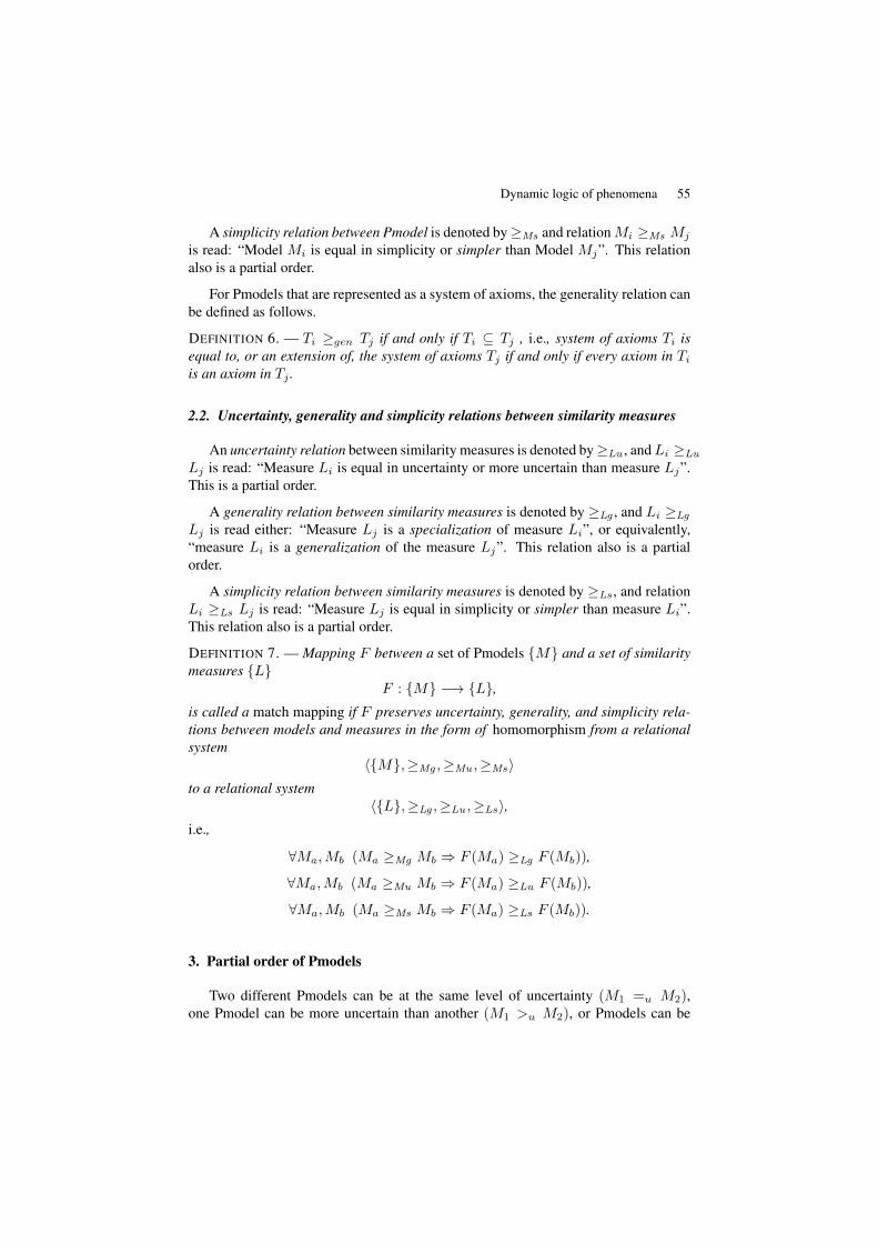
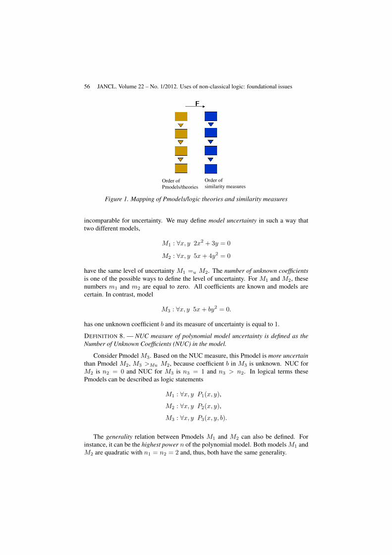
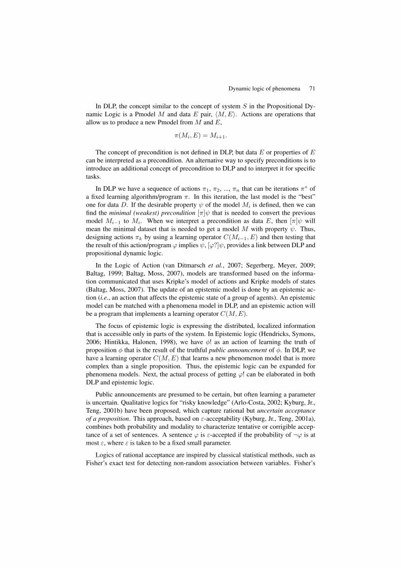
Order ofPmodels/theories

Order ofsimilarity measures

Figure 1. Mapping of Pmodels/logic theories and similarity measures

incomparable for uncertainty. We may define model uncertainty in such a way thattwo different models,

M1 : ∀x, y 2x2 + 3y = 0

M2 : ∀x, y 5x+ 4y2 = 0

have the same level of uncertainty M1 =u M2. The number of unknown coefficientsis one of the possible ways to define the level of uncertainty. For M1 and M2, thesenumbers m1 and m2 are equal to zero. All coefficients are known and models arecertain. In contrast, model

M3 : ∀x, y 5x+ by2 = 0.

has one unknown coefficient b and its measure of uncertainty is equal to 1.

DEFINITION 8. — NUC measure of polynomial model uncertainty is defined as theNumber of Unknown Coefficients (NUC) in the model.

Consider Pmodel M3. Based on the NUC measure, this Pmodel is more uncertainthan Pmodel M2, M3 >Mu M2, because coefficient b in M3 is unknown. NUC forM2 is n2 = 0 and NUC for M3 is n3 = 1 and n3 > n2. In logical terms thesePmodels can be described as logic statements

M1 : ∀x, y P1(x, y),

M2 : ∀x, y P2(x, y),

M3 : ∀x, y P3(x, y, b).

The generality relation between Pmodels M1 and M2 can also be defined. Forinstance, it can be the highest power n of the polynomial model. Both modelsM1 andM2 are quadratic with n1 = n2 = 2 and, thus, both have the same generality.


DEFINITION 9. — HP measure of polynomial model generality is defined as theHighest Power n of the polynomial model.

Alternatively, we may look deeper and notice thatM1 contains x2 andM2 containsy2. We may then define the generality of a polynomial model as its highest polynomialvariable, which are x2 for M1 and y2 for M2.

If the interpretations of x and y are fixed and cannot be swapped, then we cannotsay that one is more general than the other and we can call them incomparable ingenerality.

The described measures are computed separately for each individual model ratherthan for a pair of models to be compared. As a result, the measures may not representan intuitive generality order relation between models. For instance, we can call modelM3 more general than model M2, M3 >Mg M2, because M2 is a specialization ofM3 with b = 4. Similarly, intuitively the Pmodel

M4 : ∀x, y ax+ cx2 + by2 = 0

is more general than Pmodels M1, M2, and M3, because coefficients in M1, M2 andM3 are different numeric specializations of a, b, and c in M4.

However,

HP(M1) = HP(M2) = HP(M3) = HP(M4) = 2;

that is, all of these Pmodels have the same HP generality, whileM4 is intuitively moregeneral than the other models.

Thus, alternatively, we may define the generality of a polynomial model as itshighest polynomial variable, which is x2 for M1 and y2 for M2. If the interpretationsof x and y are fixed and we cannot swap symbols x and y, then we cannot say thatone of them is more general than the other. Thus, they would be incomparable ingenerality.

DEFINITION 10. — HPV measure of polynomial model generality is defined as theHighest Power Variable (HPV) of the polynomial model.

For models M1 and M2 we have HPV(M1) = x2 and HPV(M2) = y2. If thereare two HPV as in model M = 2x2 + 4x + 3y2 + 5y = 0, then HPV(M) is a pair(x2, y2). In the case with more than two HPVs we will have an n-dimensional vectorof HPVs.

Below we discuss the advantages and disadvantages of HP and HPV measures. Ifwe cannot fix the meaning of the variables x and y, or if we cannot even agree to useonly the symbols x and y, then HPV may not be an appropriate measure.

Swapping symbols will lead to HPV(M1) = y2 and HPV(M2) = x2. Usingother symbols such as z and v instead of x and y will make a use of HPV even morequestionable.


As we discussed above, intuitively M3 seems more general than M2, and M4

seems more general than models M1, M2, and M3. The HPV measure captures thisbetter with

HPV(M1) = x2, HP(M2) = y2, HP(M3) = y2, HP(M4) = (x2, y2).

M4 is more general than the other models in HPV, but model M3 is more generalthan M2, which is a special case of M3 with b = 4. This is not captured by HPV,

HPV(M2) = HPV(M3) = y2.

Therefore, we introduce another generality characteristic that is defined on pairs ofmodels.

DEFINITION 11. — Polynomial model Mi is a coefficient specialization (C-specialization) of a polynomial model Mj if coefficients of Mi are specializationsof coefficients of Mj . In other words, Mj is a C-generalization of model Mi.

For instance, Pmodel M3 is a C-specialization of model M4. Similarly, M2 is aC-specialization of M3, but M1 is not C-specialization of M2.

Note that model M4 is more uncertain than models M1, M2, and M3, because allcoefficients in M4 are uncertain, but none of the coefficients are uncertain in M1, M2,and only one coefficient is uncertain in M3.

DEFINITION 12. — SP measure of polynomial model simplicity is defined as the Sumof Powers of its variables. For instance, SP(M3) = 3 having powers 1 and 2 in5x1 + by2. One model is SP-simpler than the other if its SP measure is smaller. HereM3 is simpler than M4 , which has SP = 5.

Uncertainty, generality, and simplicity relations can be isomorphic (produce thesame order of Pmodels), or be quite different. In the next section, we provide a pa-rameterization mechanism that highlights the difference.

4. Parameterization

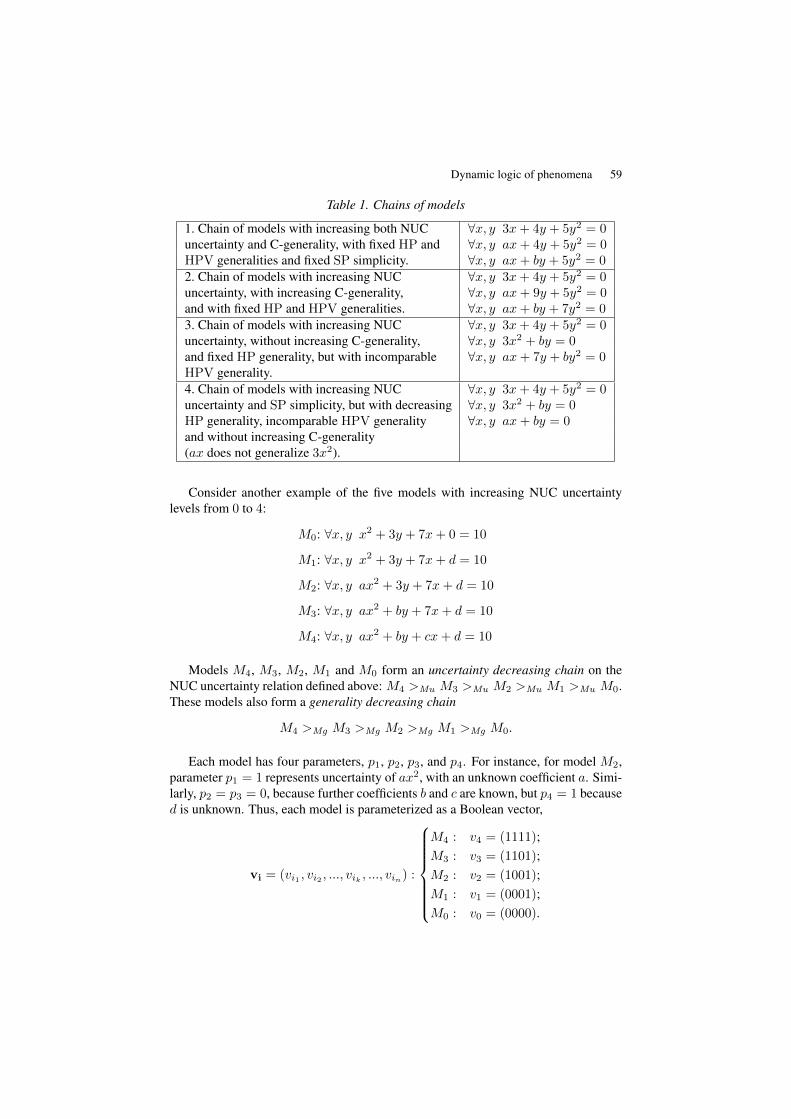
Below we parameterize uncertainty and generality of polynomial models. The firstblock in Table 1 shows a chain of models with increasing NUC uncertainty, (from 0 to2), fixed HP generality, (2), fixed HPV generality, (y2), and increasing C-generality:that is, from all known coefficients to two unknown coefficients, a and b, that substitutecoefficients 3 and 4, respectively.

All these models have HP level 2 and SP simplicity level equal to 4. Other blocksin Table 1 illustrate other relations between these characteristics of the models.


Table 1. Chains of models

1. Chain of models with increasing both NUC ∀x, y 3x+ 4y + 5y2 = 0uncertainty and C-generality, with fixed HP and ∀x, y ax+ 4y + 5y2 = 0HPV generalities and fixed SP simplicity. ∀x, y ax+ by + 5y2 = 02. Chain of models with increasing NUC ∀x, y 3x+ 4y + 5y2 = 0uncertainty, with increasing C-generality, ∀x, y ax+ 9y + 5y2 = 0and with fixed HP and HPV generalities. ∀x, y ax+ by + 7y2 = 03. Chain of models with increasing NUC ∀x, y 3x+ 4y + 5y2 = 0uncertainty, without increasing C-generality, ∀x, y 3x2 + by = 0and fixed HP generality, but with incomparable ∀x, y ax+ 7y + by2 = 0HPV generality.4. Chain of models with increasing NUC ∀x, y 3x+ 4y + 5y2 = 0uncertainty and SP simplicity, but with decreasing ∀x, y 3x2 + by = 0HP generality, incomparable HPV generality ∀x, y ax+ by = 0and without increasing C-generality(ax does not generalize 3x2).

Consider another example of the five models with increasing NUC uncertaintylevels from 0 to 4:

M0: ∀x, y x2 + 3y + 7x+ 0 = 10

M1: ∀x, y x2 + 3y + 7x+ d = 10

M2: ∀x, y ax2 + 3y + 7x+ d = 10

M3: ∀x, y ax2 + by + 7x+ d = 10

M4: ∀x, y ax2 + by + cx+ d = 10

Models M4, M3, M2, M1 and M0 form an uncertainty decreasing chain on theNUC uncertainty relation defined above: M4 >Mu M3 >Mu M2 >Mu M1 >Mu M0.These models also form a generality decreasing chain

M4 >Mg M3 >Mg M2 >Mg M1 >Mg M0.

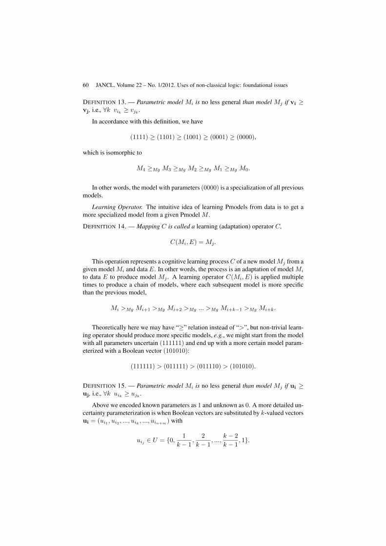
Each model has four parameters, p1, p2, p3, and p4. For instance, for model M2,parameter p1 = 1 represents uncertainty of ax2, with an unknown coefficient a. Simi-larly, p2 = p3 = 0, because further coefficients b and c are known, but p4 = 1 becaused is unknown. Thus, each model is parameterized as a Boolean vector,

vi = (vi1 , vi2 , ..., vik , ..., vin) :

M4 : v4 = (1111);M3 : v3 = (1101);M2 : v2 = (1001);M1 : v1 = (0001);M0 : v0 = (0000).


DEFINITION 13. — Parametric model Mi is no less general than model Mj if vi ≥vj, i.e., ∀k vik ≥ vjk .

In accordance with this definition, we have

(1111) ≥ (1101) ≥ (1001) ≥ (0001) ≥ (0000),

which is isomorphic to

M4 ≥Mg M3 ≥Mg M2 ≥Mg M1 ≥Mg M0.

In other words, the model with parameters (0000) is a specialization of all previousmodels.

Learning Operator. The intuitive idea of learning Pmodels from data is to get amore specialized model from a given Pmodel M .

DEFINITION 14. — Mapping C is called a learning (adaptation) operator C,

C(Mi, E) = Mj .

This operation represents a cognitive learning processC of a new modelMj from agiven model Mi and data E. In other words, the process is an adaptation of model Mi

to data E to produce model Mj . A learning operator C(Mi, E) is applied multipletimes to produce a chain of models, where each subsequent model is more specificthan the previous model,

Mi >Mg Mi+1 >Mg Mi+2 >Mg ... >Mg Mi+k−1 >Mg Mi+k.

Theoretically here we may have “≥” relation instead of “>”, but non-trivial learn-ing operator should produce more specific models, e.g., we might start from the modelwith all parameters uncertain (111111) and end up with a more certain model param-eterized with a Boolean vector (101010):

(111111) > (011111) > (011110) > (101010).

DEFINITION 15. — Parametric model Mi is no less general than model Mj if ui ≥uj, i.e., ∀k uik ≥ ujk .

Above we encoded known parameters as 1 and unknown as 0. A more detailed un-certainty parameterization is when Boolean vectors are substituted by k-valued vectorsui = (ui1 , ui2 , ..., uik , ..., uin+m

) with

uij ∈ U = 0, 1

k − 1,

2

k − 1, ...,

k − 2

k − 1, 1.


5. Similarity maximization

A similarity maximization problem is a major mechanism of DLP that is formal-ized below.

DEFINITION 16. — A similarity Lfin measure is called a final similarity measure if:

∀M,E,Li Li(M,E) ≥Lu Lfin(M,E).

The final similarity measure specifies the level of certainty of model similarity tothe data that we want to reach.

DEFINITION 17. — The static model optimization problem (SMOP) is to find a modelMa such that

Lfin(Ma, E) = maxj∈J

Lfin(Mj , E) (1)

subject to conditions (2) and (3):

∀Mj ∈ U(Ma) Lfin(Ma, E) = Lfin(Mj , E)⇒Ma ≥Mu Mj (2)

∀Mj ∈ G(Ma) Lfin(Ma, E) = Lfin(Mj , E)⇒Ma ≥Mg Mj (3)

The goal of (2) and (3) is to prevent model overfitting with data E. Sets U(Ma)and G(Ma) contain Pmodels that are comparable with Ma relative to uncertainty andgenerality, respectively. Condition (2) means that if Ma and Mj have the same sim-ilarity measure with E, then uncertainty of Ma should be no less than uncertainty ofMj . Condition (3) expresses an analogous condition for the generality relation. Toospecific models can lead to overfitting.

DEFINITION 18. — The dynamic logic model optimization (DLPO) problem is to finda Pmodel Ma such that

La(Ma, E) = maxj∈J

Lj(Mj , E) (4)

subject to conditions (5) and (6):

∀Mj ∈ U(Ma) La(Ma, E) = Lj(Mj , E)⇒Ma ≥Mu Mj (5)

∀Mj ∈ G(Ma) Lj(Ma, E) = Lj(Mj , E)⇒Ma ≥Mg Mj (6)

This is a non-standard optimization problem. In standard optimization problems,only modelsMi are changed but the optimization criterionL is held fixed, since it doesnot depend on the model Mi. In DLP, however, the criterion L changes dynamicallywith Pmodels Mj .

Since the focus of DLP is cutting computational complexity (CC) of model opti-mization, a dual optimization problem can be formulated.


DEFINITION 19. — An optimization problem of finding a shortest sequence ofmatched pairs (Mi, Li) of Pmodels Mi and optimization criteria (similarity mea-sures) Li that solves the optimization problem (4)–(6) for the given data E is calleda dual dynamic logic model optimization (DDLMO) problem, which finds a sequenceof n matching pairs

(M1, L1), (M2, L2), ..., (Mn, Ln),

such thatLn(Mn, E) = max

i∈ILi(Mi, E)

and

∀Mi Li = F (Mi), C(Mi, E) = Mi+1,

Mi ≥Mu Mi+1, Mi ≥Mg Mi+1, Mn = Ma, Ln = La.

This means finding a sequence of more specific and certain Pmodels for the given(1) data E, (2) matching operator F , and (3) learning operator C to maximize simi-larity measure Li(Mi, E).

6. Monotone Boolean functions

DEFINITION 20. — A Boolean function f : 0, 1n −→ 0, 1 is a monotoneBoolean function if: vi ≥ vj ⇒ f(vj) ≥ f(vi).

This means that (vi ≥ vj & f(vi) = 0) ⇒ f(vj) = 0 and (vi ≥ vj & f(vj) =1) ⇒ f(vi) = 1. Function f is non-decreasing. Consider fixed E and Mi thatare parameterized by vi and interpret L(Mi, E) as f(vi), i.e., L(Mi, E) = f(vi).Assume that L(Mi, E) has only two values (unacceptable 0, and acceptable 1). It canbe generalized to a k-value case if needed. If L(Mi, E) is monotone, then vi ≥ vj ⇒L(Mi, E) ≥ L(Mj , E), e.g., if L(M3−1110, E) = L(M2−1100, E) = 0, then

(vi ≥ vj &L(M3−1110, E) = 0)⇒ L(M2−1100, E) = 0 (7)

(vi ≥ vj &L(M2−1100, E) = 1)⇒ L(M3−1110, E) = 1 (8)

This means that if a model with more unknown parameters vi failed, then a modelwith less unknown parameters vj will also fail. If we conclude that a quadratic poly-nomial model (M2) is not acceptable, L(M2, E) = 0, then a more specific quadraticmodel M3 also cannot be acceptable, L(M3, E) = 0. Thus, we do not need to testmodel M3. This monotonicity property helps to decrease computational complexity.We use

(vi ≥ vj & f(vi) = 0)⇒ f(vj) = 0 (9)

or rejecting models, and

(vi ≥ vj & f(vj) = 1)⇒ f(vi) = 1 (10)


for confirming models. In the case of a model rejection test for data E, the focus isnot to quickly build a model but rather to quickly reject a model M—in the spirit ofPopper’s falsification principle.

In essence, the test L3(M3, E) = 0 means that the whole class of models M3

with 3 unknown parameters fails. Testing M3 positively for data E requires find-ing 4 correct parameters. This may mean searching in a large 4-D parameter space[−100,+100]4 for a single vector, say (p1, p2, p3, p4) = (9, 3, 7, 10), if each param-eter varies in the interval [−100, 100]. For rejection we may need only 4 trainingvectors (x, y, u) from data E and 3 other test vectors. The first four vectors allow usto build a quadratic surface in 3-D as a model. We then simply test whether three testvectors from E fail to fit this quadratic surface.

7. Search process

In the optimization process, we want to keep track of model rejections and to guidedynamically what model will be tested next in order to minimize the number of tests.Formulas (9) and (10) are key equations to minimize tests, but we need the wholestrategy for how to minimize the number of tests and to formalize it. This strategy isformalized as minimization of Shannon function ϕ, which was proposed in (Hansel,1966):

minA∈A

maxf∈F

ϕ(f,A),

where A is a set of algorithms, F is a set of monotone functions, and ϕ(f,A) is anumber of tests that algorithm A does to fully restore function f . Each test meanscomputing a value f(v) for a particular vector v. In the theory of monotone Booleanfunctions it is assumed that there is an oracle that is able to produce the value f(v),thus each test is equivalent to a request to the oracle (Hansel, 1966; Kovalerchuk,Vityaev, 2000; Kovalerchuk et al., 1996). Minimization of the Shannon functionmeans that we search for the algorithm that needs the smallest number of tests forits worst case (function f that needs maximum number of tests relative to other func-tions). This is a classic min-max criterion. It was proved in (Hansel, 1966) that

minA∈A

maxf∈F

ϕ(f,A) =

(nbn2 c

)+

(n

bn2 c+ 1

),

where bxc is the floor of x. The proof is based on the structure called Hansel chains.These chains cover the whole n-dimensional binary cube 1, 0n. The steps of the al-gorithm are presented in detail in (Kovalerchuk, Delizy, 2005; Kovalerchuk, Vityaev,2000).

The main idea of these steps is building Hansel chains, starting from testing thesmallest chains, expanding each tested value using formulas (7) and (8), testing valuesthat are left unexpanded on the same chains, then moving to larger chains until nochains are left. The goal of the search is to find a smallest lower unit v, i.e., a Booleanvector such that f(v) = 1, and for every w < v, f(w) = 0, and for every u > v,|u| > |v|. A simpler problem could be to find any lower unit of f .


The search problem in logical terms can be formulated as a satisfiability problem:Find a system of axioms Ta such that La(Ta, E) = 1 subject to the condition

∀Tj La(Ta, E) = Lj(Tj , E)⇒ Tj ≥Mu Ta,

i.e., if Ta and Tj have the same similarity with E, then Ma should have a lower uncer-tainty than Tj , e.g., Tj ≥Mu Ta. If a similarity measure L is defined as a probabilisticmeasure in [0, 1] then the probabilistic version of finding a system of axioms T formodel A that maximizes a probabilistic similarity measure is:

maxi∈I

L(Mi, E).

8. Dynamic logic visualization

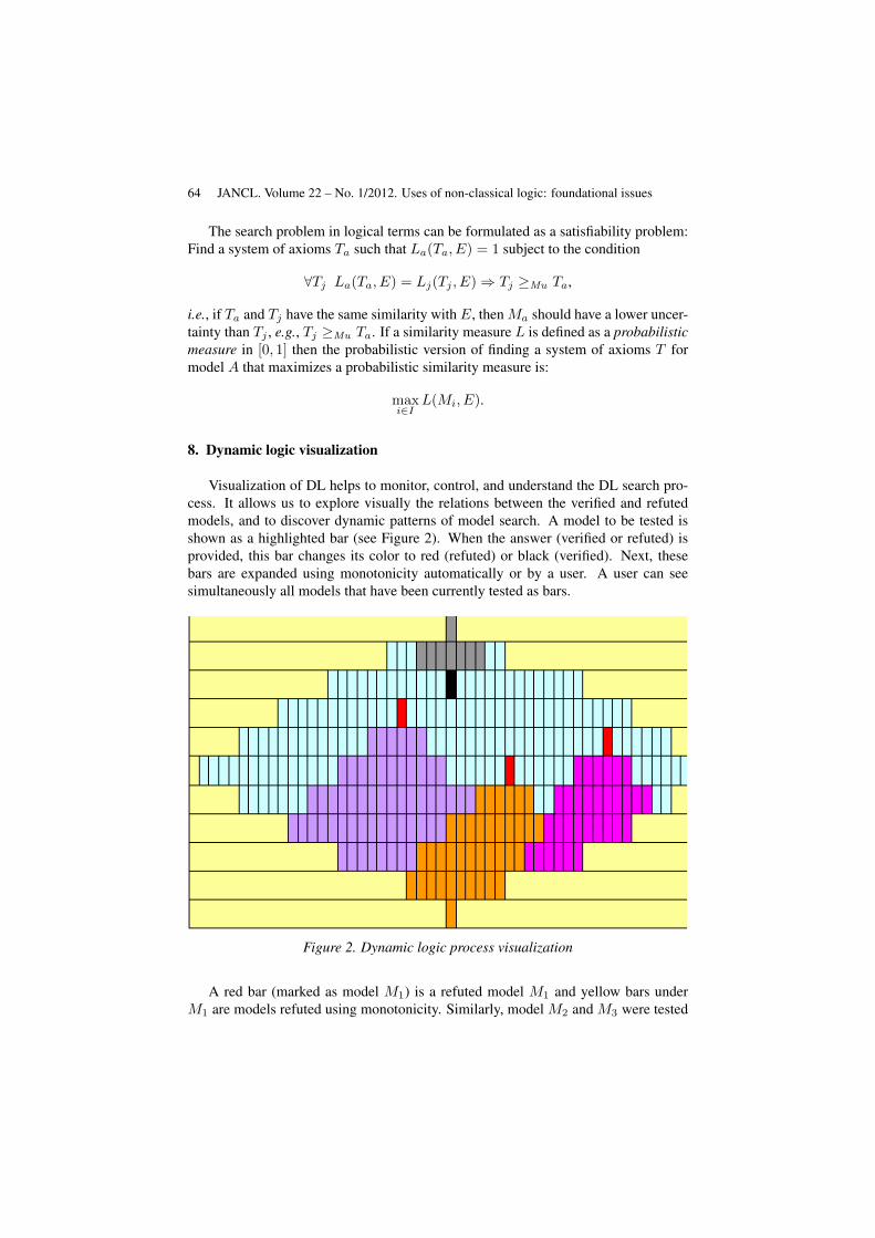
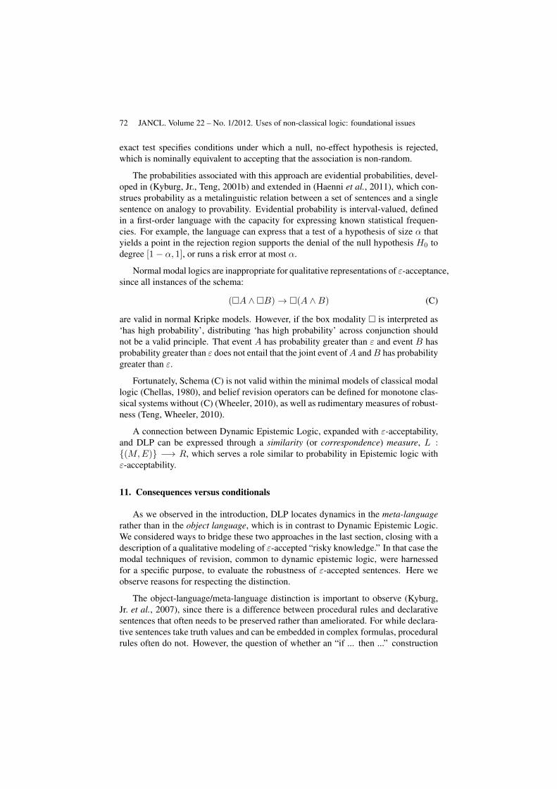
Visualization of DL helps to monitor, control, and understand the DL search pro-cess. It allows us to explore visually the relations between the verified and refutedmodels, and to discover dynamic patterns of model search. A model to be tested isshown as a highlighted bar (see Figure 2). When the answer (verified or refuted) isprovided, this bar changes its color to red (refuted) or black (verified). Next, thesebars are expanded using monotonicity automatically or by a user. A user can seesimultaneously all models that have been currently tested as bars.

Figure 2. Dynamic logic process visualization

A red bar (marked as model M1) is a refuted model M1 and yellow bars underM1 are models refuted using monotonicity. Similarly, model M2 and M3 were tested


next and refuted, which is indicated by their red bar. Colored bars below them arealso refuted using monotonicity. Then model M4 was verified and encoded by a blackbar with all models verified using monotone expansion of M4 are shown above M4 asgrey bars. Using technique from (Kovalerchuk, Delizy, 2005), bars can be rearrangedto reveal their pattern as a Pareto set/border (see Figure 2). The border is dynamicallydeveloped as more models are tested. Finally, a user will see a border between verifiedand refuted models and can impose additional requirements to monitor border modelsthat satisfy such additional requirements.

9. Formal description of P-dynamic logic

Below we describe formally our dynamic logic of models of phenomena (DLP) asa summarization of concepts introduced above. As with any logic, DLP consists ofthree parts: (1) a semantic part, (2) a syntactic part, and (3) a reasoning part.

9.1. Semantic part of DLP

At first, we define the semantic part of DLP. It consists of two related algebraicsystems. The first one is a three-sort algebraic system (Malcev, 1973), where E aresets of data, M are sets of Pmodels, R is the set of real numbers,

EM = 〈E, M, R; ΩEM 〉. (11)

ΩEM consists of sets of relations, ΩE , ΩPM , ΩR on E, M and R, respectively,and operators L and C that connect E, M and R,

ΩEM = 〈ΩE ,ΩPM ,ΩR, L, C〉. (12)

Here ΩPM = ≥Mg ,≥Mu ,≥Ms presents partial order relations between Pmod-els relative to their generality, uncertainty and simplicity as described above. Eachsimilarity (correspondence) measure Li ∈ L is a mapping:

Li : M × E −→ R. (13)

A similarity measure captures numerically the similarity between data and Pmod-els. A higher value of Li(M,E) indicates a higher consistency between data E andthe Pmodel M in the aspect that was captured by Li. Having a set of such measuresL allows us to choose appropriate measures dynamically.

Next, a Pmodel enhancement (learning) operator C is

C : M,E −→ M (14)

that changes a Pmodel. This operator brings us dynamics of model changes. Thus,we have two types of dynamics and we need a formal way to express the change of Lsimilar to (14) for models. This is done by introducing a two-sort algebraic system

ML = 〈M, L; ΩPM ,ΩL, F 〉, (15)


with

ΩPM = ≥Mg ,≥Mu ,≥Ms, ΩL = ≥Lg ,≥Lu,

and F as a mapping between sets M and L that preserves relations on M,

F : M −→ L. (16)

Algebraic systems (11) and (15) have several common components, but L hasvery different roles in each. In (11), L is part of Ω, i.e., it is an operator; butin (15) L is one of two base sets of the algebraic system, where the operator isF : M −→ L.

Thus, we cannot simply join systems (11) and (15) together to a single algebraicsystem because of the different roles played by L in (11) and (15). We would needa generalized multi-sort algebraic system in second order-logic to do this. Note thatseparately (11) and (15) are much simpler systems in first-order logic (FOL).

In addition, we can build (15) without a specific dataset E ∈ E, because (15)does not require E. To construct (11) for a specific dataset E, we would need todefine ΩE . See an extensive discussion of these issues and examples in (Krantz et al.,1971; Kovalerchuk, Vityaev, 2000). Thus, the semantic part of the DLP is

EMML = 〈EM,ML;W 〉,

where W (Mi, E,Mj) is the following relation that consists of three parts (17)–(19):

W (Mi, E,Mj) ≡

([C ∈ ΩEM &C(Mi, E) = Mj ] & (17)

[(Mi >u Mj) ∨ (Mi >g Mj) ∨ (Mj >s Mi)]∨ (18)

[Li = F (Mi) &Lj = F (Mj) &Lj(Mj , E) > Li(Mi, E)]). (19)

Relation W (Mi, E,Mj) is true if and only if C produces a Pmodel Mj using Ethat is better than the input Pmodel Mi in at least one of its characteristics (i.e., morecertain, more specific, simpler, or better fit data relative to similarity measures). Inother words, a Boolean predicate W (Mi, E,Mj) = 1 if C(Mi, E) = Mj producesan improved model Mj , otherwise W (Mi, E,Mj) = 0.

In accordance with the definitions in previous sections, in (18)Mi >Mu Mj meansthat Mj is a more certain model than Mi. Similarly, Mi >Mg Mj means that Mj isa more specific, and Mj >s Mi means that Mj is simpler than Mi. Property (19)means that model Mj better fits data E than model Mi relative to measures Lj andLi, which are dynamically assigned to Mj and Mi by applying F to them.

Not every operator that produces another model can be called a learning operator.Relation W sets up a semantic criterion for operator C to be a learning operator for


Pmodels Mi, Mj and data E. Note that (17) and (18) in W can be checked havingonly EM, but (19) requires ML too.

Now we want to discuss how to compute truth-values of predicates and outputsof operators in EM and ML. For EM and ML we gave some examples of ΩM

and ΩL, L, C and F . An extensive set of examples of similarity measures L andlearning operators C are given in (Perlovsky, 2000). For ML in addition we need tocompute F . For instance, if M(c, r) is a model that represents a circle with centerc and radius r, then L(c, r) could be the same, F (M(c, r)) = L = M(c, r). Thismeans that L tests exactly model M(c, r). An alternative F could be F (M(c, r)) =L = M(c, r + e) that accepts all models with radiuses no greater than r + e.

In general a library of such matching operators F and relations ΩM and ΩL shouldbe created that will be available to researchers. Thus, we have a semantic part of theP -dynamic logic identified.

9.2. Syntactic part of P-dynamic logic

Now we need to explore which part of this semantic machinery can be transferredto the syntactic level so that we can do reasoning without semantic knowledge to getat least some non-trivial inferences and conclusions.

To distinguish the syntactic level from the semantic level, we will use low-casenotation em and ml to define the syntactic structure of EM and ML, respectively.We do this for all components; thus,

em = 〈e, m, r;ωem〉. (20)

The ωem consists of sets of relations ωe, ωm, ωr on e, m and r, respectively,and operators l and c that connect e, m and r,

ωem = 〈ωe, ωm, ωr, l, c〉 (21)

Similarly, we define

ml = 〈m, l;ωm, ωl, f〉, (22)

that includes

ωm = ≥mg ,≥mu ,≥ms, ωl = ≥lg ,≥lu, f : m −→ l (23)

Similarly, we define emml = 〈em,ml;w〉, where

w(mi, e,mj) ≡([c ∈ ωem & c(mi, e) = mj ] (24)

[(mi >mu mj) ∨ (mi >mg mj) ∨ (mj >ms mi)]∨ (25)

[li = f(mi) & lj = f(mj) & lj(mj , e) > li(mi, e)]). (26)


9.3. Reasoning part of DLP

Now we will discuss the reasoning part of DLP. To build a reasoning deductivesystem for DL we need a set Λ of logical axioms, a set Σ of non-logical axioms, and aset Γ, ϕ of rules of inference.

It will be interesting to explore if it is complete, i.e., for all formulas ϕ,

If Σ |= ϕ then Σ ` ϕ.

If this system is actually incomplete, then we will have statement ϕ such thatneitherϕ nor¬ϕ can be proved from the given set of axioms. In contrast, in a completesystem, all true statements (made true by the set of axioms) are provable.

We also need to know the validity of the inference rules; that is, we need to estab-lish that the conclusion follows from the premises. The soundness of these rules needsto be clarified, too; that is, it needs to be shown that the conclusion follows from thepremises when the premises are in fact true.

While all these are interesting research issues, at this stage of formalization of DLPit is more important to have first a rich set of useful non-logical axioms Σ. To clarifythis issue we need to answer the following questions: What reasoning is possible inDLP? What could be the most interesting part of syntactic reasoning for a specificpractical problem?

Assume that we already have a knowledge base (KB). This KB contains m1,...,mn, and e that are called facts in this KB (m1, ..., mn are interpreted semanticallyas Pmodels and e as data). KB also contains some expressions, e.g., w(mi, e,mj)(interpreted semantically as Pmodel mj is an improved Pmodel mi).

For the first series of questions we have common first-order reasoning with logicalaxioms Λ that use ∧, ∨, ¬, and ⇒ operators. Non-logical axioms Σ include thedisjunction axiom (DA) and conjunction axiom (CA) and mixed CDA axiom:

CA: w(mi, e1,mk) ∨ w(mi, e2,mk)⇒ w(mi, e1 ∪ e2,mk),

DA: w(mi, e1,mk) ∧ w(mi, e2,mk)⇒ w(mi, e1 ∩ e2,mk),

DCA: w(mi, e1,mk) ∧ w(mi, e2,mk)⇒ w(mi, e1 ∪ e2,mk).

The last axiom is redundant if we add the inclusion axiom (IA):

IA: w(mi, e1 ∩ e2,mk)⇒ w(mi, e1 ∪ e2,mk).

Together DA and IA produce DCA. The real world interpretation of these axioms willassume some regularity in data and learning operators.

Next we want to know if w(mi, e,mk) can be inferred purely syntactically know-ing that w(mi, e,mj) and w(mj , e,mk) are in the KB but without using a semanticinterpretation of w(mi, e,mk). By having this we will have useful syntactic reason-


ing in this DL. In fact, a transitivity axiom (TA) can be established as part of a set ofnon-logical axioms Σ,

TA: w(mi, e,mj) ∧ w(mj , e,mk)⇒ w(mi, e,mk).

It follows from the semantics of relation W that it is transitive, thus we can postu-late transitivity for w. As a result of this postulate we can infer w(mi, e,mk) purelysyntactically having w(mi, e,mj) and w(mj , e,mk) in KB without going to the se-mantic level and computing W (Mi, E,Mk), which can be computationally challeng-ing for a large dataset E. This is a major advantage of using DLP syntactic reasoninginstead of computations at the semantic level.

The reasoning mechanism Tem in em is a first-order logic with terms in its sig-nature. Similarly, Tml in ml it is a first-order logic in terms of its signature. In〈em,ml;w〉 we have Temml that is also a first-order logic reasoning with w, but ifwe substitute w with its components (24)–(26), we will have second-order logic rea-soning. Thus, the complete description of the dynamic logic of phenomena modelsis

DL = 〈DLEM ,DLML,DLEMML〉,

where

DLEM = 〈em, Tem ,EM〉,DLML = 〈ml , Tml ,ML〉,DLEMML = 〈emml, Temml ,EMML〉.

9.4. Learning operator

Now we want to elaborate the concept of a learning operator, C. There is animportant question about this operator: How sophisticated should C be relative to abrute force algorithm that computes L(M,E) for every PmodelM and selectsM thatprovides minL(M,E)?

It will be advantageous to get a simple and quite universal operator, C, whichwill allow us to use it for solving a wide variety of problems. Let us consider adirect modification of a brute force algorithm to the situation with dynamic changeof correspondence (similarity) measures Li, which is assumed in the dynamic logic.The next assumption is that the space of highly uncertain models is relatively small.Thus, a brute force algorithm can work for these models in a reasonable time. Next,the best model M1 found at this step will produce a new correspondence measure L1

and this measure will be applied to a new set of models produced byM1 for evaluation(e.g., with a more dense grid around M1 or in another location if L(M1) is low). Toproduce new models we introduce a new operator,H , that we will call a specializationoperator, as follows:


Step 1. Select initial Pmodel M0.Step 2. Produce set of Pmodels H(M0).Step 3. Compute L0(M,E) for every M from H(M0) = M and find model

M1 = argminM L0(M,E).Step 4. Test if L0(M1, E) > T , i.e., is above the needed correspondence

threshold. Stop if it is true, else go to step 5.Step 5. Repeat steps 1–4 until all models tested or time limit reached.

More complex strategies for the H operator can be based on breadth-first, depth-first, and branch-and-bound strategies.

10. Relations with other dynamic logics

A link with the Dynamic Logic for Belief Revision (van Benthem, 2007) is feasibleto explore. The transition from model Mi to model Mj using partial orders betweenmodels can be viewed as a belief revision.

At a very general level, the link between Dynamic Logic of Phenomena and ei-ther Propositional or First-Order Dynamic Logic (Balbiani, 2007; Pratt, 1978) fol-lows from the fact that Dynamic Logic of Phenomena contains static components(propositional/first-order formulas), and dynamic components (actions/programs). Aformula can change when actions are applied, and actions can be repeated and appliedconsecutively. Thus, the Dynamic Logic of Phenomena can be viewed as a specialcase of Propositional or First-Order Dynamic Logics with special types of “programs”described in this paper.

Below we follow (Baltag, Smets, 2008) in summarizing the Propositional DynamicLogic that has been useful for capturing important properties of programs, such ascorrectness. The basic concept of this logic is the state S of a system. Each state S hasits properties expressed as a propositional formula ϕ. These properties are changedwhen a program (action) π is applied to S with a given precondition a. Thus, programπ can produce S with property ψ starting with S with property ϕ and precondition a,

π(S, a) = ψ.

Propositional formulas are static components of this logic and actions/programsare dynamic components. Actions can be applied consecutively and repeated, whichis expressed syntactically as π, π′ and π∗, respectively. An action also can be takenrandomly from a set of actions, π ∪ π′. One of the actions is testing, which is denotedby ‘ϕ?’. It tests if property ϕ is true or false for system S.

There is also an order relation (≥w) on the set of preconditions a. It expressesthe relative strength (weakness) of the precondition. The statement a1 ≥w a2 meansthat a1 is weaker than a2. [π]ϕ is the weakest precondition ψ that leads to postcondi-tion ϕ after performing π on S. Also [ϕ?]ψ denotes the classical implication ψ → ϕ,that is if S satisfies ψ then it satisfies ϕ, too.


In DLP, the concept similar to the concept of system S in the Propositional Dy-namic Logic is a Pmodel M and data E pair, 〈M,E〉. Actions are operations thatallow us to produce a new Pmodel from M and E,

π(Mi, E) = Mi+1.

The concept of precondition is not defined in DLP, but data E or properties of Ecan be interpreted as a precondition. An alternative way to specify preconditions is tointroduce an additional concept of precondition to DLP and to interpret it for specifictasks.

In DLP we have a sequence of actions π1, π2, ..., πn that can be iterations π∗ ofa fixed learning algorithm/program π. In this iteration, the last model is the “best”one for data D. If the desirable property ψ of the model Mi is defined, then we canfind the minimal (weakest) precondition [π]ψ that is needed to convert the previousmodel Mi−1 to Mi. When we interpret a precondition as data E, then [π]ψ willmean the minimal dataset that is needed to get a model M with property ψ. Thus,designing actions πk by using a learning operator C(Mi−1, E) and then testing thatthe result of this action/program ϕ implies ψ, [ϕ?]ψ, provides a link between DLP andpropositional dynamic logic.

In the Logic of Action (van Ditmarsch et al., 2007; Segerberg, Meyer, 2009;Baltag, 1999; Baltag, Moss, 2007), models are transformed based on the informa-tion communicated that uses Kripke’s model of actions and Kripke models of states(Baltag, Moss, 2007). The update of an epistemic model is done by an epistemic ac-tion (i.e., an action that affects the epistemic state of a group of agents). An epistemicmodel can be matched with a phenomena model in DLP, and an epistemic action willbe a program that implements a learning operator C(M,E).

The focus of epistemic logic is expressing the distributed, localized informationthat is accessible only in parts of the system. In Epistemic logic (Hendricks, Symons,2006; Hintikka, Halonen, 1998), we have φ! as an action of learning the truth ofproposition φ that is the result of the truthful public announcement of φ. In DLP, wehave a learning operator C(M,E) that learns a new phenomenon model that is morecomplex than a single proposition. Thus, the epistemic logic can be expanded forphenomena models. Next, the actual process of getting ϕ! can be elaborated in bothDLP and epistemic logic.

Public announcements are presumed to be certain, but often learning a parameteris uncertain. Qualitative logics for “risky knowledge” (Arlo-Costa, 2002; Kyburg, Jr.,Teng, 2001b) have been proposed, which capture rational but uncertain acceptanceof a proposition. This approach, based on ε-acceptability (Kyburg, Jr., Teng, 2001a),combines both probability and modality to characterize tentative or corrigible accep-tance of a set of sentences. A sentence ϕ is ε-accepted if the probability of ¬ϕ is atmost ε, where ε is taken to be a fixed small parameter.

Logics of rational acceptance are inspired by classical statistical methods, such asFisher’s exact test for detecting non-random association between variables. Fisher’s


exact test specifies conditions under which a null, no-effect hypothesis is rejected,which is nominally equivalent to accepting that the association is non-random.

The probabilities associated with this approach are evidential probabilities, devel-oped in (Kyburg, Jr., Teng, 2001b) and extended in (Haenni et al., 2011), which con-strues probability as a metalinguistic relation between a set of sentences and a singlesentence on analogy to provability. Evidential probability is interval-valued, definedin a first-order language with the capacity for expressing known statistical frequen-cies. For example, the language can express that a test of a hypothesis of size α thatyields a point in the rejection region supports the denial of the null hypothesis H0 todegree [1− α, 1], or runs a risk error at most α.

Normal modal logics are inappropriate for qualitative representations of ε-acceptance,since all instances of the schema:

(A ∧B)→ (A ∧B) (C)

are valid in normal Kripke models. However, if the box modality is interpreted as‘has high probability’, distributing ‘has high probability’ across conjunction shouldnot be a valid principle. That event A has probability greater than ε and event B hasprobability greater than ε does not entail that the joint event ofA andB has probabilitygreater than ε.

Fortunately, Schema (C) is not valid within the minimal models of classical modallogic (Chellas, 1980), and belief revision operators can be defined for monotone clas-sical systems without (C) (Wheeler, 2010), as well as rudimentary measures of robust-ness (Teng, Wheeler, 2010).

A connection between Dynamic Epistemic Logic, expanded with ε-acceptability,and DLP can be expressed through a similarity (or correspondence) measure, L :(M,E) −→ R, which serves a role similar to probability in Epistemic logic withε-acceptability.

11. Consequences versus conditionals

As we observed in the introduction, DLP locates dynamics in the meta-languagerather than in the object language, which is in contrast to Dynamic Epistemic Logic.We considered ways to bridge these two approaches in the last section, closing with adescription of a qualitative modeling of ε-accepted “risky knowledge.” In that case themodal techniques of revision, common to dynamic epistemic logic, were harnessedfor a specific purpose, to evaluate the robustness of ε-accepted sentences. Here weobserve reasons for respecting the distinction.

The object-language/meta-language distinction is important to observe (Kyburg,Jr. et al., 2007), since there is a difference between procedural rules and declarativesentences that often needs to be preserved rather than ameliorated. For while declara-tive sentences take truth values and can be embedded in complex formulas, proceduralrules often do not. However, the question of whether an “if ... then ...” construction


is better viewed as a conditional formula than as a conditional rule, or whether thereis little difference between the two and an analogue of the deduction theorem can beused, is not always clear cut, and will depend on the purpose of the formalization.

To illustrate, input/output logic (Makinson, van der Torre, 2000; 2001) was con-ceived as a response to deontic logics handling of norms and declarative statements.Norms, unlike statements, may be respected or flouted, and may be judged from thestandpoint of other norms but are not typically evaluated as ‘true’ or ‘false’. In-put/output logic conceives of a norm as an ordered pair of formulas, and a norma-tive system is a set G of norms. The task for an input/output logic, then, is to pre-pare information to be passed into G, and to unpack the resulting output. So, ab-stractly, the set G is a transformation devise for information, and we may characterizean ‘output’ operator Out by logical properties typical of consequence operators. Aformula x is a ‘simple-minded output’ of G in context a, written x ∈ Out(G, a),if there is a set of norms (a1, x1), ..., (an, xn) in G such that each ai ∈ Cn(a) andx ∈ Cn(x1 & ...&xn), where Cn(a) = ai | a |= ai is the classical semantic con-sequence set of a that is a set of all contexts ai such that every model of a is also amodel of ai (Makinson, van der Torre, 2000).

Out(G, a) satisfies three rules: writing (a, x) for x ∈ Out(G, a), they are strength-ening input (SI), conjoining output (AND), and weakening output (WO):

From (a, x) to (b, x), whenever a ∈ Cn(b). (SI)

From (a, x), (a, y) to (a, x ∧ y). (AND)

From (a, x) to (a, y), whenever y ∈ Cn(x). (WO)

Strengthening input means that if context a leads to output x then a stronger context balso leads to x. Similarly, weakening output means that if context a leads to output xthen context a also leads to a weaker output y, x |= y, that is y ∈ Cn(x).

Here the idea is that, while classical logic may be used to ‘process’ the input andto ‘unpack’ the output, the operator Out itself does not have either an associated lan-guage or a proof theory. Even so, Out may enjoy structural properties commonlyattributed to consequence operators. Simple-minded output is the most general char-acterization of Out , but stronger input/output operators have been studied (Makinson,van der Torre, 2000), including a characterization of Poole’s default system (Poole,1988), and a system similar to Reiter’s default logic (Reiter, 1980).

EXAMPLE 21 (from (Boella et al., 2009)). — Suppose there are two communitynorms governing social benefits, one which maintains that poor citizens receive ahousing subsidy, and the other that elderly citizens receive health insurance, i.e.,G = (Poor,SubsidizedHousing), (Elderly,HealthInsurance). Then, the commu-


nity should also provide a housing subsidy if no-income implies poor is included inthe theory, i.e.,

SubsidizedHousing ∈ Out(G, (NoIncome→ Poor) & NoIncome), since

Poor ∈ Cn((NoIncome→ Poor) & NoIncome) and

SubsidizedHousing ∈ Cn(SubsidizedHousing).

While one may agree that deontic logic has traditionally mishandled norms, it isnot clear that there is anything essential about norms, which would preclude themfrom being represented by a statement within a language (Wheeler, Alberti, 2011).The point instead is that we must first understand the system we wish to model beforedefining the language we need, rather than the other way around.

A good illustration of this point is the theory of causal modeling (Pearl, 2000;Spirites et al., 2000), since “if ... then ...” statements have long been thought to expressa causal relationship between events. Whereas in normative systems the main issue isthe apparent non-truth-functional character of norms, the issues with causal modelingconcern the asymmetrical nature of causal relationships and, more importantly, therole that intervention plays in our understanding of causal relationships.

Certainly, logics of conditionals have abounded; most attempt to ground condi-tionals of this kind in the semantic features of the mood, aspect, and tense of naturallanguage conditional statements. And some philosophical theories of causality haveattempted to build from these studies in formal semantics.

However, in the case of causal modeling, success came once the order of inquirywas reversed. While both equational and causal models rely upon symmetrical equa-tions to describe a system, causal models in addition impose asymmetries by assumingthat each equation corresponds to an independent mechanism, which may be manipu-lated.

The theory of causal Bayesian networks (Pearl, 2000; Spirites et al., 2000) sup-plied the mathematical framework for causal modeling, and it did so by ignoring thetask of formulating a calculus and focused instead on getting the right mathematicalframework. Only recently has there been a proposal for a calculus, and the clarityof Judea Pearl’s causal algebra of ‘doing’ (Boella et al., 2009) relies upon this back-ground theory.

12. Conclusion and future work

This paper has introduced a formalization of the dynamic logic of phenomena inthe terms of first-order logic, logic model theory, and the theory of Monotone Booleanfunctions. This formalization covers the main idea of DLP: matching levels of uncer-tainty of the problem/model to levels of uncertainty of the evaluation criterion, whichdramatically decreases computation complexity of finding a model.


The core of the formalization is a partial order on the phenomena models andsimilarity measures with respect to their uncertainty, generality, and simplicity. Thesepartial orders are represented using a set of Boolean parameters within the theory ofmonotone Boolean functions and can be visualized in line with (Kovalerchuk, Delizy,2005) to monitor and guide the search in the Boolean parameter space in the DLsetting.

Further studies are needed to establish a richer set of non-logic axioms and toexplore validity, soundness, and completeness of expanded DLP. Such studies mayreveal deeper links with classical logic problems such as decidability, completeness,and consistency.

Further theoretical studies may find deeper links with classical optimization searchprocesses, and may significantly advance them by adding an extra layer of optimiza-tion criteria constructed dynamically. This work also gives a new perspective formachine learning (De Raedt, 2006; Kovalerchuk, Vityaev, 2000) to develop learningalgorithms that can learn evaluation criteria and models simultaneously. We expectthat deep links with a known Dynamic Logic of programs (Harel et al., 2000) moti-vated by logical analysis of computer programs will also be established.

The proposed formalization creates a framework for developing specific applica-tions and modeling tools. We envision a modeling tool that will consist of sets ofmodels, matching similarity measures, processes for testing them and model learn-ing processes for specific problems in pattern recognition, data mining, optimization,cognitive process modeling, and decision making.

From our viewpoint, the most interesting and useful future DLP research is dis-covering a mechanism for changing models and similarity measures. Humans havedemonstrated capabilities to switch evaluation criteria instantaneously in dynamic en-vironments (Perlovsky, 2007), and more generally are able to exploit noncompen-satory processing strategies to draw inferences (Gigerenzer et al., 1999; Katsikopou-los, Martignon, 2006). This is the area where logic, mathematical modeling, and cog-nitive science can provide mutual benefits in discovering mechanisms for changingmodels and changing similarity measures.

References

Arlo-Costa H. (2002). First order extensions of classical systems of modal logic: the role ofthe barcan schemas. Studia Logica, Vol. 71, No. 1, pp. 87–118.

Balbiani P. (2007). Propositional dynamic logic. Stanford Encyclopedia of Philosophy.(http://plato.stanford.edu/entries/logic-dynamic/)

Baltag A. (1999). A logic of epistemic actions. In W. van der Hoek, J.-J. Meyer, C. Wit-teveen (Eds.), Foundations and applications of collective agent-based systems, proceedingsof the workshop at the 11th european summer school in logic, language, and computation.Utrecht, Available online in PDF.

Baltag A., Moss L. S. (2007). Logics for epistemic programs. Synthese, Vol. 139, pp. 165–224.


Baltag A., Smets S. (2008). A dynamic-logical perspective on quantum behavior. StudiaLogica, Vol. 89, pp. 187–211.

van Benthem J. (1996). Exploring logical dynamics. Stanford, CSLI Publications.

van Benthem J. (2007). Dynamic logic for belief revision. Journal of Applied Non-ClassicalLogics, Vol. 17, No. 2, pp. 129–155.

van Benthem J. (2009). Personal communications.

Boella G., Pigozzi G., van der Torre L. (2009). Normative framework for normative systemchange. In Proc. of 8th int. conf. on autonomous agents and multiagent systems (aamas2009). AAAI Press.

Chellas B. (1980). Modal logic. New York, Cambridge University Press.

De Raedt L. (2006). From inductive logic programming to multi-relational data mining.Springer.

van Ditmarsch H., van der Hoek W., Kooi B. (2007). Dynamic epistemic logic (Vol. 337).Springer.

van Gelder T. (1995). What might cognition be, if not computation? Journal of Philosophy,Vol. 91, pp. 345–381.

Gigerenzer G., Todd P. M., The ABC Research Group (Eds.). (1999). Simple heuristics thatmake us smart. New York, Oxford University Press.

Haenni R., Romeijn J.-W., Wheeler G., Williamson J. (2011). Probabilistic logics and proba-bilistic networks (Vol. 350). Springer.

Hansel G. (1966). Sur le nombre des fonctions Booléennes monotones de n variables. Compte-rendu de l’Académie des Sciences de Paris, Vol. 262, No. 20, pp. 1088–1090.

Harel D., Kozen D., Tiuryn J. (2000). Dynamic logic. Cambridge, MA, MIT Press.

Hendricks V., Symons J. (2006). Epistemic logic. Stanford Encyclopedia of Philosophy.(http://plato.stanford.edu/entries/logic-epistemic/)

Hintikka J., Halonen I. (1998). Epistemic logic. In Routledge encyclopedia of philosophy,Vol. 1, pp. 752–753. London, Routledge.

Hodes W. (2005). First-order model theory. Stanford Encyclopedia of Philosophy.(http://plato.stanford.edu/entries/modeltheory-fo/)

Katsikopoulos K. V., Martignon L. (2006). Naive heuristics for paired comparison : Someresults on their relative accuray. Journal of Mathematical Psychology, Vol. 50, pp. 488–494.

King J. C. (2004). Context dependent quantifiers and donkey anaphora. In M. Ezcurdia,R. Stainton, C. Viger (Eds.), New essays in the philosophy of language, supplement tocanadian journal of philosophy, Vol. 30, pp. 97–127. Calgary, Alberta, Canada, Universityof Calgary Press.

Kovalerchuk B., Delizy F. (2005). Visual data mining using monotone boolean functions. InB. Kovalerchuk, J. Schwing (Eds.), Visual and spatial analysis: Advances in data mining,reasoning, and problem solving, pp. 387–406. Springer.


Kovalerchuk B., Triantaphyllou E., Despande A., Vityaev E. (1996). Interactive learning ofmonotone boolean function. Information Sciences, Vol. 94, pp. 87–118.

Kovalerchuk B., Vityaev E. (2000). Data mining in finance: Advances in relational and hybridmethods. Dordrecht, Kluwer.

Krantz D. H., Luce R. D., Suppes P., Tversky A. (1971). Foundations of measurement. NewYork, Academic Press.

Kyburg, Jr. H. E., Teng C. M. (2001a). The logic of risky knowledge (Vol. 67). Elsevier.

Kyburg, Jr. H. E., Teng C. M. (2001b). Uncertain inference. New York, Cambridge UniversityPress.

Kyburg, Jr. H. E., Teng C. M., Wheeler G. (2007). Conditionals and consequences. ournal ofApplied Logic, Vol. 5, No. 4, pp. 638–650.

Leitgeb H. (2009). Personal communications.

Leitgeb H., Segerberg K. (2007). Dynamic doxastic logic: why, how, and where to? Synthese,Vol. 155, pp. 167–190.

Makinson D., van der Torre L. (2000). Input/output logics. Journal of Philosophical Logic,Vol. 29, pp. 383–408.

Makinson D., van der Torre L. (2001). Constraints for input/output logics. Journal of Philo-sophical Logic, Vol. 30, pp. 155–185.

Malcev A. (1973). Algebraic systems. Springer-Verlag.

Pearl J. (2000). Causality: Models, reasoning, and inference. Cambridge, Cambridge Univer-sity Press.

Perlovsky L. (2000). Neural networks and intellect: Using model-based concepts. Oxford,Oxford University Press.

Perlovsky L. (2006). Toward physics of the mind: Concepts, emotions, consciousness, andsymbols. Physics of Life Review, Vol. 3, pp. 23–55.

Perlovsky L. (2007). Evolution of language, consciousness, and cultures. IEEE ComputationalIntelligence Magazine, Vol. 8, pp. 25–39.

Pitt D. (2008). Mental representation. Stanford Encyclopedia of Philosophy.(http://plato.stanford.edu/entries/mental-representation/)

Pojman P. (2009). Ernst mach. Stanford Encyclopedia of Philosophy.(http://plato.stanford.edu/entries/ernst-mach/)

Poole D. (1988). A logical framework for default reasoning. Artificial Intelligence, Vol. 36,pp. 27–47.

Pratt V. (1978). A practical decision method for propositional dynamic logic. In Proceedingsof the 10th annual acm symposium on theory of computing, pp. 326–337. ACM.

Reiter R. (1980). A logical framework for default reasoning. Artificial Intelligence, Vol. 13,pp. 81–132.

Segerberg K., Meyer J.-J. (2009). The logic of action. Stanford Encyclopedia of Philosophy.(http://plato.stanford.edu/entries/logic-action/)


Spirites P., Glymour C., Scheines R. (2000). Causation, prediction, and search (2nd ed.).Cambridge, MA, MIT Press.

Teng C., Wheeler G. (2010). Robustness of evidential probability. In E. Clarke, A. Voronkov(Eds.), Short paper proceedings of international conference on logic for programming, ar-tificial intelligence, and reasoning (lpar-16). Springer.

Wheeler G. (2010). AGM belief revision in monotone modal logics. In E. Clarke, A. Voronkov(Eds.), Short paper proceedings of international conference on logic for programming, ar-tificial intelligence, and reasoning (lpar-16). Springer.

Wheeler G., Alberti M. (2011). NO revision and NO contraction". Minds and Machines,Vol. 21, No. 3, pp. 411–30.


Annex A. Polynomial complexity case

Below we describe two examples that give computational motivation to our re-search on building a logical formalism for representing the dynamic logic of phenom-ena.

The first example is about finding a model to fit a hidden circle in noisy data whenthe level of noise is so high that a direct human observation does not allow a visualclue about the location of the circle within the image.

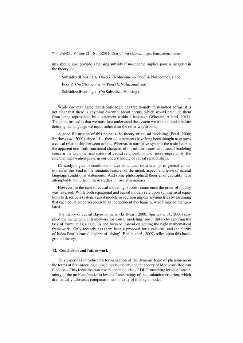
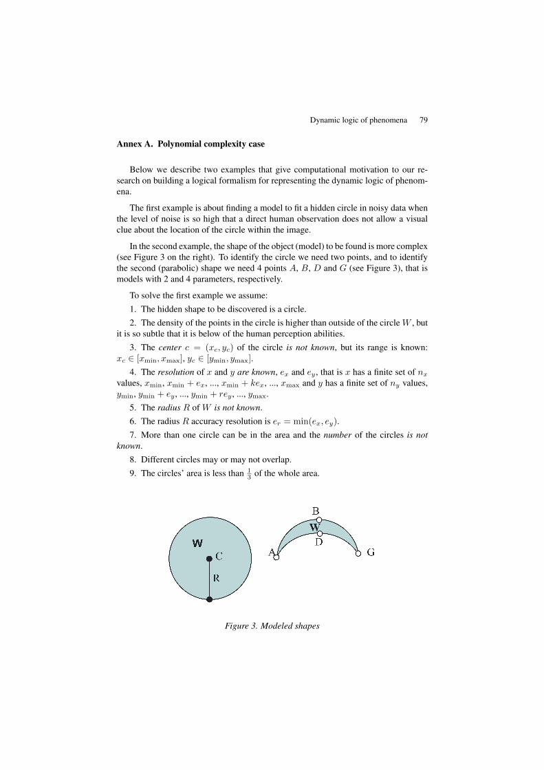
In the second example, the shape of the object (model) to be found is more complex(see Figure 3 on the right). To identify the circle we need two points, and to identifythe second (parabolic) shape we need 4 points A, B, D and G (see Figure 3), that ismodels with 2 and 4 parameters, respectively.

To solve the first example we assume:1. The hidden shape to be discovered is a circle.2. The density of the points in the circle is higher than outside of the circle W , but

it is so subtle that it is below of the human perception abilities.3. The center c = (xc, yc) of the circle is not known, but its range is known:

xc ∈ [xmin, xmax], yc ∈ [ymin, ymax].4. The resolution of x and y are known, ex and ey , that is x has a finite set of nx

values, xmin, xmin + ex, ..., xmin + kex, ..., xmax and y has a finite set of ny values,ymin, ymin + ey , ..., ymin + rey , ..., ymax.

5. The radius R of W is not known.6. The radius R accuracy resolution is er = min(ex, ey).7. More than one circle can be in the area and the number of the circles is not

known.8. Different circles may or may not overlap.9. The circles’ area is less than 1

3 of the whole area.

Figure 3. Modeled shapes


The brute force algorithm for example 1 conducts Density Difference Test forevery node C = (xc, yc) and everyR on the grid. It returns 1 if D(R)−D(¬R) > T ,else 0, that is if density D(W ) in circle W is greater than D(¬W ) with threshold T ,where D(¬W ) is density outside W . Here The Computational Complexity (CC) ofthis algorithm with the base operation as Density Difference Test (C,R) is O(n3) ona square grid n× n.

The CC of Density Difference Test function is defined by the total number m ofgiven points with the base operation as testing (xi−xc)2 + (yi−xc)2 ≤ R2, that is ifthe point is inside of the circle. The total computational complexity of the brute forcealgorithm is O(n3m). If input points covers the whole grid, then m = n and CC isequal to O(n4). If fact m is a fraction of n, thus if m = n

10 , then we still have O(n4).

Now we will change our assumption 1, i.e., that the hidden shape to be discoveredis a circle. A more complex shape to discover is produced by two quadratic curvesshown in Figure 3. Three points, A, B, and G, are sufficient to identify the first curve,and three points, A, D, and G, are sufficient to identify the second curve. Thus, intotal 4 points are sufficient to identify both curves. In the case of the circle, we needonly two points, center C, and any point H on the circle.

To solve the task for our new parabolic shape, we keep the same assumptions aswe had for the circle. We assume the unknown number of shapes of unknown sizes,locations, and orientations.

Complexity of a brute force algorithm is O(n4) which is greater than for Example1 due to a greater number of parameters involved. The density difference test has thesame complexity O(m) as above for the circle, but is more complex for points insideof the shape.

However, this test’s time grows linearly with m. For each point, it computes twoquadratic forms and tests if the point is in or out of the shape based on these values.This time is limited by a constant for each given point. Thus, the total complexityis O(n4m), and if m would reach n, then it will be O(n5). While these algorithmsare polynomial, they have limited applicability for data of practical sizes as we showbelow.

Assume that m = n10 , thus our complexity functions for examples 1 and 2 are

k1(n4

10 ) and k2(n5

1 ), respectively. We also assumed 109 base operations/sec in thesecomputations. Note that this base operation is a part of the Density Difference Testcomputed for each of m inputs.

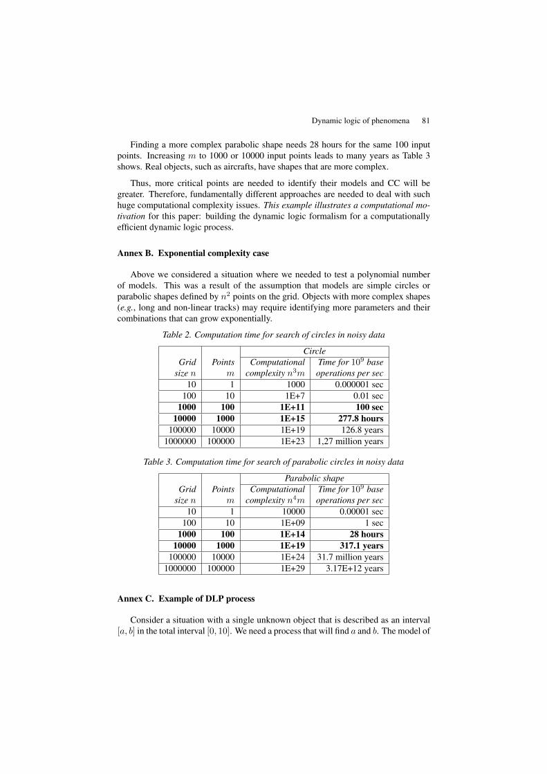
Table 2 and Table 3 show computational complexity under these assumptions forsearch of circles and parabolic shapes. A computer screen grid of pixels is about1000×1000 and images from current cameras are larger. Only for a single screen with100 input points, finding the circle has an acceptable time (100 sec) which also can betoo slow for real time applications.


Finding a more complex parabolic shape needs 28 hours for the same 100 inputpoints. Increasing m to 1000 or 10000 input points leads to many years as Table 3shows. Real objects, such as aircrafts, have shapes that are more complex.

Thus, more critical points are needed to identify their models and CC will begreater. Therefore, fundamentally different approaches are needed to deal with suchhuge computational complexity issues. This example illustrates a computational mo-tivation for this paper: building the dynamic logic formalism for a computationallyefficient dynamic logic process.

Annex B. Exponential complexity case

Above we considered a situation where we needed to test a polynomial numberof models. This was a result of the assumption that models are simple circles orparabolic shapes defined by n2 points on the grid. Objects with more complex shapes(e.g., long and non-linear tracks) may require identifying more parameters and theircombinations that can grow exponentially.

Table 2. Computation time for search of circles in noisy data

CircleGrid Points Computational Time for 109 base

size n m complexity n3m operations per sec10 1 1000 0.000001 sec

100 10 1E+7 0.01 sec1000 100 1E+11 100 sec

10000 1000 1E+15 277.8 hours100000 10000 1E+19 126.8 years

1000000 100000 1E+23 1,27 million years

Table 3. Computation time for search of parabolic circles in noisy data

Parabolic shapeGrid Points Computational Time for 109 base

size n m complexity n4m operations per sec10 1 10000 0.00001 sec

100 10 1E+09 1 sec1000 100 1E+14 28 hours

10000 1000 1E+19 317.1 years100000 10000 1E+24 31.7 million years

1000000 100000 1E+29 3.17E+12 years

Annex C. Example of DLP process

Consider a situation with a single unknown object that is described as an interval[a, b] in the total interval [0, 10]. We need a process that will find a and b. The model of


the object is [a, b], which is highly uncertain because both values a and b are unknownand only limited by the interval [0, 10]. Thus, the first class of models is M = [a, b] :a, b ∈ [0, 10].

To be specific, assume that the unknown object (model) is the interval [0, 4]. Thismodel has center c = 2 and radius r = 2, and can be written as [a, b] = m(c, r). Letalso M(c,R) = m(c, r) be a set of all models with center c and radiuses r that areno greater than R. Consider a set of all models (intervals) M(c, 5) with all radiusesr ≤ 5. Here c and r also are highly uncertain.

Now we build at first a very uncertain evaluation measure (criterion) L0 for thisclass of models M(c,R) and data E as a kernel function. For instance, consider aGaussian distribution, N(5, 10), where c = 5 is a mean and r = 10 is a standarddeviation. This standard deviation is two times greater than the largest R = 5 inthe [0, 10] interval, thus it covers M(c, 5) models (intervals) and should not fail forthis class of models. This means that the result of applying L0 based on N(5, 10) toM(c, 5) is positive, L0(M(c, 5)) = 1. This indicates that an object exists in [0, 10],but its location is uncertain. We still do not know exactly c and r, but the class ofmodels M(c, 5) is confirmed because we have L0(M(c, 5)) = 1.

Having this positive result, the next step is to change the similarity measure L, tomake it less uncertain, by substituting L0 = N(5, 10) by, say, L1 based on N(5, 7).This substitution can be done by using a learning operator. Testing L1 on M(c, 5)is not a computational challenge. It can be done quickly, which is a major benefit ofDLP. This quick process of changing L and M is repeated until it reaches the level ofmaximum certainty of models that is possible on available data. This process is muchfaster than a brute force approach described in previous examples in this appendix.Here for simplicity of exposition we assumed that L takes binary values. For morecomplex non-binary L see (Perlovsky, 2000; 2006).

For the actual use of the DLP methodology, elaborated classes of models and crite-ria need to be developed at the matched level of uncertainty. Some of them are alreadydeveloped in likelihood function terms (Perlovsky, 2000; 2006).

Documents

Modeling phenomena and dynamic logic of phenomena