Ph ton 175

The Journal of Ecology. Photon 107 (2013) 175-189 https://sites.google.com/site/photonfoundationorganization/home/the-journal-of-ecology Original Research Article. ISJN: 6853-3275

The Journal of Ecology Ph ton

Modeling the Effect of Gestation Delay of Predator on the Stability of Bifurcating Periodic Solutions in Wetland Ecosystem D. Jana

a, N. Bairagi

a, R. Agrawal

b, R.K. Upadhyay

b*

a Department of Mathematics, Jadavpur University, Kolkata - 700032, India

b Department of Applied Mathematics, Indian School of Mines, Dhanbad - 826004, Jharkhand, India

Article history: Received: 28 March, 2013 Accepted: 08 May, 2013 Available online: 20 July, 2013 Keywords: Good and bad biomass, predator, gestation delay, stability, limit cycle, Hopf bifurcation Corresponding Author: Upadhyay R.K. * Email: ranjit_ism@yahoo.com Phone & Fax No: +913262296563

Abstract We investigate the effect of gestation delay of predator on the stability of the coexisting equilibrium of a wetland model for Keoladeo National Park. It is

observed that there is a stability switches, and Hopf bifurcation occurs when the delay crosses some critical value. By applying the normal form theory and the center manifold theorem, the explicit formulae which determine the stability and direction of the bifurcating periodic solutions are determined. Computer simulations have been carried out to illustrate different analytical findings. Results indicate that the Hopf bifurcation is subcritical and the bifurcating periodic solution is unstable for the considered parameter. Citation: Jana D., Bairagi N., Agrawal R., Upadhyay R.K., 2013. Modeling the Effect of Gestation Delay of Predator on the Stability of Bifurcating Periodic Solutions in Wetland Ecosystem. The Journal of Ecology. Photon 107, 175-189.

1. Introduction

A wetland ecosystem is a complex system in which abiotic ingredients like water, nutrients and light are abundant but free oxygen is limited. Wetlands are regulators of water regimes. Recently, the significance of wetland and its biodiversity has been understood in proper ecological perspective (Vijayan, 1991; Cairns, 1992), classification and procedures of its management have been outlined (Finlayson, 1991). Some well known wetland types are (Rai et al., 2011) (i) Constructed wetlands, (ii) Fresh water wetlands and (iii) Flood plain wetlands. Vijayan (1991) has studied different aspects of ecology of the park. A mathematical model was proposed by Shukla and Dubey (1996) to study the effect of ecological changes caused by excessive growth of wild grasses such as Paspalum distichum on the existence of various species in Keoladeo National Park (KNP) at Bharatpur, Rajesthan, India. Shukla (1998) have reinvestigated the model of Shukla and Dubey (1996) with the help of the regression analysis of the observed biomass data for the Paspalum distichum and other aquatic macrophytes. They also suggested the proper management and effort required to control the wild grasses.

Middleton (1998) offered a contrasting view to Shukla and Dubey’s model (1996) which advocates the introduction of water buffalo in the KNP to remove wild grasses, specifically Paspalum distichum and shown that it was unsupported by field research. Chopra and Adhikari (2004) used a simulation modeling approach to examine the links between economic and ecological value of KNP over a thirty year time. Srinivasu and Chopra (2004) have proposed the 3D model of KNP consisting of good biomass, bad biomass and the bird population. Rai (2008) modeled the dynamics of the biotic part of the wetland system of KNP and also suggested for improvement of wetland with the help of 2D scan diagrams and time series. Rai et al. (2011) have applied this model to study the science and technology for the water quality management. In this paper, we have extended the model studied by Rai (2008) and Rai et al. (2011) by adding time delay in the predator response function, popularly known as gestation delay, and study the effects of this gestation delay of predator ( i.e., bird ) popula- tion on the stability of the coexisting equilibrium point. We have also explored the direction and stability of bifurcating periodic

Ph ton 176

solutions of the proposed delay induced model of Keoladeo National Park. The organization of the paper is as follows: Section 2 describes the dynamics of the biotic system of the wetland part of KNP. Section 3 deals with the linear stability analysis of the delay-induced system. In section 4, direction and stability of Hopf bifurcation are presented. Numerical results to illustrate the analytical findings are discussed in section 5 and finally, a conclusion is presented in section 6. 2. The Mathematical Model System With reference to migratory birds, the biomass is divided into two categories: “Good” and “Bad”. The paspalum and its family acts as a bad biomass for the birds and the floating vegetation. The following species of the floating vegetation, Nymphoidesindicum, Nymphoides- cristatum, Nymphaeanouchali, Nymphaeastellat, and other useful species are categorized as “good” biomass (Shukla and Dubey, 1996). The fishes and the water fowl are the most suffered species. The excess growth of the wild grass species, Paspalum distichum restricts the growth of bulbs, tubers and roots, on which avifauna feeds on. Paspalum distichum is known to deplete oxygen in the natural aquatic systems is the dominant species. The economic value of the park is dependent on tourist activities. The tourists are mainly attracted by Siberian Crane, the migratory bird which adds aesthetic value to KNP. Although visits of the tourists bring revenue to the state, it also creates a disturbance gradient to the system. We consider the following wetland model for the KNP:

In this model, G, B, P represents the densities of good biomass, bad biomass and bird population (both resident and migratory birds), respectively. Here r and 1r are the reproductive growth rates, K and K1 are the carrying capacities of the environment for good and bad biomass, respectively. The ratio of K1 and 1r represents the per capita water availability of bad biomass B. The parameters b and b1 measure the intensities of competition between good and bad biomass.

ω is the maximum rate at which the bird population consumes the good biomass and d

is the half- saturation constant. 1ω is the

maximal gain in bird biomass and θ is the death rate of bird population in absence of food. Mathematicians frequently use different types of delays to represent biological events more accurately. An excellent review work of predator-prey models with different discrete delays can be seen in Ruan (2009). In model system (1.1), we consider a time delay τ in the predator response function. This delay can be regarded as a gestation period or reaction time of the predator (Kuang, 1993). Our model (1.1) in presence of gestation delay reads as

We study the delay-induced system (1.2) with the following initial conditions:

Hopf bifurcation and its stability in a delay-induced predator-prey system have been studied by many researchers (Ruan, 2001; Wen et al., 2002; Liu et al., 2009; Yang et al., 2005; Qu et al., 2007; Celik, 2008). In this paper, we study the effect of gestation delay of predator on the stability of a wetland model of KNP and find the direction and stability of the bifurcating periodic solutions, if any. 3. Stability Analysis The model system described by (1.1) possesses six nonnegative real equilibrium points: (i) the trivial equilibrium point

0( 0 , 0 , 0 )E = always exists. The eigenvalue

of the Jacobian matrix around 0E are

1, a n d .r r θ− thus, the trivial equilibrium is

always unstable.

(ii) The equilibrium point 1( , 0 , 0 )E K= exists

on the boundary of the first octant. 1E is

stable if 1 1 1, / ( )r b K w K K d θ< + < .

(iii) The equilibrium point 2 1( 0 , , 0 )E K=

exists on the boundary of the first octant. E2 is

asymptotically stable if 1r b K< .

Ph ton 177

(iv) Equilibrium point 3( , , 0 )E G B= % %

is the

planer equilibrium point on the GB -plane, where

1 1 1 1 1

1 1 1 1 1 1

( ) ( ),

( ) ( )

K r r b K r K r b KG B

r r b b K K r r b b K K

− −= =

− −% %

. If 1 1 1r r b b K K> , 1 1r b K> then the equilibrium

point 3( , , 0 )E G B% %

is stable or unstable in the positive direction orthogonal to GB-plane, i.e. P direction, depending on whether

1

3

w G

G dλ θ= − +

+

%

% is negative or positive

respectively, provided that 1 1 1r r b b K K> .

(v) The equilibrium point 4( , 0 , )E G P=% %% %

is

the planer equilibrium point on the GP -plane, where

1

1

, 1 ( ) .( )

d r GG P G d

w w K

θ

θ

= = − + −

%%% %%% %%

The

equilibrium point ( , 0 , )G P% %% %

is stable or unstable in positive direction orthogonal to GP-plane, i.e. B direction, depending on

whether 1 1r b G−

%%is negative or positive

respectively provided that 2

( )w P K r G d< +%% %% .

(vi) The interior equilibrium point is given by

E*(G*,B*,P*), where 1

dG

θ

ω θ∗ =

− ,

( )1

1 1

1

KB r b G

r

∗ ∗= −

and

( )1 .

r K GGP b B

K

ω

θ ω

∗∗∗ ∗

− = −

This equilibrium point will be biologically feasible if

1

1b d

rθ

+

< 1ω

<

( )1 1

1 1

1d b b K K r

b r K Kθ

− +

and

r < ( )1 1 1/ .b K K r b d d+

2.1 Theorem Suppose that the positive equilibrium point E* = (G*, B*, P*) of the model system (1.1) exists. The equilibrium point E* =(G*, B*, P*) is locally asymptotically stable if and only if the following conditions hold:

* * 2

( ) ;KwP r G d< +

* 2 * * 2

1 1 1 1( ) ( ) .bb KK G d Kwr P rr G d+ + < +

Now, we are going to discuss the stability of the model system (1.2) around the

coexistence equilibrium E*. Let ( )x t = ( )G t G

∗− , ( ) ( )y t B t B∗= − ,

( ) ( )z t P t P ∗= − are the perturbed variables. Then the system (1.2) can be expressed in the matrix form after linearization as follows:

where

( )

* * * *

*

2 **

*

1

1 1

1

0

0 0 0

G P rG GbG

K d Gd G

r BA b B

K

ω ω

∗

− − −

++ = − −

and 2A

= ( )

*

1

2*

0 0 0

0 0 0

0 0dP

d G

ω

+ .

The characteristic equation of the system (2.1) is given by

i.e., Equation (2.3) can be written as

Here

For 0τ = , Eq. (2.4) becomes

where Following Routh-Hurwitz criterion, the roots of (2.5) will have negative real parts if P, Q, R

and P Q R− are positive. One can easily verify that these conditions are satisfied if Theorem 2.1 holds. We now reproduce some definitions given by (Kuang, 1993; Brauer, 1987). 2.1 Definition The equilibrium E* is called asymptotically stable if there exists a δ > 0 such that

Ph ton 178

implies that

where ( ) ( ) ( )( ), ,G t B t P t

is the solution of the system (1.2) which satisfies the condition (1.3). 2.2 Definition The equilibrium E* is called absolutely stable if

it is asymptotically stable for all delays 0τ ≥

and conditionally stable if it is stable for τ in some finite interval. Note that the system (1.2) will be stable around the equilibrium E* if all the roots of the corresponding characteristic Eq. (2.4) have negative real parts. But Eq. (2.4) is a transcendental equation and has infinite number of roots. It is difficult to determine the sign of these infinite numbers of roots. Therefore, we study the distribution of roots of the cubic exponential polynomial Eq. (2.4).

We know that iω (ω > 0) is a root of (2.4) if

and only if ω satisfies

Separating real and imaginary parts, we get

, These two equations give the positive values

of τ and ω for which Eq. (2.4) can have purely imaginary roots. Squaring and adding these equations, we have

6 4 20p q sω ω ω+ + + =

, (2.8) where

2

2Qp P= −,

2 2

Qq R= −,

(2.8)'

2

s S= − .

If we assume2

h ω= , (2.8) reduces to 3 2

0h ph qh s+ + + =. (2.9)

Denote

( ) 3 2g h h ph qh s= + + +. (2.10)

Note that ( )0g s=

and( )lim

hg h

→+∞= +∞

.

Since s < 0, the Eq. (2.10) has at least one positive root.

2.1 Lemma Since s < 0, the Eq. (2.9) has at least one positive root. Without loss of generality, we assume that it has three positive roots, defined by h1, h2 and h3, respectively. Then, Eq. (2.8) has three

positive roots 1 1hω =

, 2 2hω =

and

3 3hω =

. From (2.7), we have

( ).3,2,1,

Qsin

22

2

3

=+

+−= k

SR

SSRP

k

kkk

ω

ωωτω

Thus, if we denote

( )

+

+

+−= π

ω

ωω

ωτ j

SR

SSRP

k

kk

k

j

k 2Q

arcsin1

22

2

3

, (2.13)

where 1,2,3k =

; 0,1, 2,j = K

., then kiω±

is a pair of purely imaginary roots of the Eq. (2.4). Define

( )

{ }

( ){ }0 0

1,2 ,3

0 0

0 0min ,k

k k kτ τ τ ω ω∈

= = =(2.14)

We reproduce the following result due to Ruan and Wei (2001) to analyse (2.4). 2.2 Lemma Consider the exponential polynomial

( ) ( ) ( ) ( )10 0 01

1 1, , , m n n

n nM e e p p p

λτλτλ λ λ λ−− −

−= + + + +K K

( ) ( ) ( ) 11 1 11

1 1

n

n np p p e

λτλ λ −−

− + + + + K

+K( ) ( ) ( )1

1 1,mm m mn

n np p p e

λτλ −−

− + + + + K

where ( )0 1, 2, ,

ii mτ ≥ = K

and ( )

,i

jp

(0,1, 2,i =

, ; 1, 2, ,m j n=K K) are constants. As

( )1 2, , ,

mτ τ τK

vary, the sum of the order of

zeros of ( )1, , , mM e e

λτλτλ −−K

on the open right half hand can change only if a zero appears on or crosses the imaginary axis. Using Lemma 2.2, we obtain the following results on the distribution of roots of the transcendental Eq. (2.4).

Ph ton 179

2.3 Lemma

As s < 0, all roots with positive real parts of the Eq. (2.4) has the same sum as those of

the polynomial Eq. (2.5) for all 0[0, )τ τ∈

. Let

( ) ( ) ( )iλ τ η τ ω τ= +, (2.15)

where η

and ω are real, be the roots of the

Eq. (2.4) near ( )j

kτ τ=

satisfying

( )( ) 0j

kη τ =

. &

( )( )j

k kω τ ω=

. Then the following transversality condition holds. 2.4 Lemma

Suppose that 2

k kh ω= and ( )' 0k

g h ≠ , where

( )g h is defined by (2.10). Then,

( )( ){ }Re 0j

k

d

dλ τ

τ ≠ , and the sign

of

( )( ){ }Rej

k

d

dλ τ

τ is consistent with that

of ( )'

kg h

. Proof. Differentiating Eq. (2.4 ) with respect to

,τ we obtain

( )23 2 Q

dP Re e R S

d

λτ λτ λλ λ τ λ

τ− − + + + − +

( )R S e λτλ λ −= +. This gives

( )( ) ( )

21 3 2 QP ed R

d R S R S

λτλ λλ τ

τ λλ λ λ λ

− + + = + −

+ +

(2.16) It follows from (2.7) that

( ) ( )

2

j

k

k kR S R i Sτ τ

λ λ ω ω=

+ =− +

,

( )( ) ( )

23 2 Q

j

k

P eλτ

τ τλ λ

=+ + =

(( )2

3 cosj

k k kω ω τ−

( ) ( )2 sin Q cos

j j

k k k k kPω ω τ ω τ− +

)

i+ (( )2

3 sin Qj

k k kω ω τ− +

( ) ( )

sin 2 cosj j

k k k k kPω τ ω ω τ+

) (2.17) Using (2.17) in (2.16), we get

( ){ } ( )

( )( ) ( )

21 3 2 Q

Re Rej

k

j

k

P ed

d R S

λτ

τ τ

τ τ

λ λλ τ

τ λ λ

−

=

=

+ + = +

( ) ( )

( )

Re Rej

kj

k

R

R S τ ττ τ

τ

λλ λ ==

+ − +

( ) ( )2 2 26 4 21

3 2 2Q Qk k kP Rω ω ω = + − + − Λ

6 4 213 2

k k kp qω ω ω = + + Λ

( )1

'k kh g h=Λ ,

where

2 24 2

k kR Sω ωΛ = +

( > 0 ). Thus, we have

( )( )

( )( )

1

R e R ej j

k k

d dsig n sig n

d dτ τ τ τ

λ τ λ ττ τ

−

= =

=

( )'0k

k

hs i g n g h

= ≠

Λ . Since Λ , kh are

positive, we conclude that the sign of

( )( )

R ej

k

d

d τ τ

λ ττ =

is determined by that of

( )'k

g h. This proves the lemma.

From ( 2 .4 ) ' and (2.8) '

, we have 2

2Qp P= −,

2 2

Qq R= −.

(2.18) Thus, from Lemmas 2.4 and 2.5, we have the following theorem. 2.2 Theorem

Let , , , ,P Q R S

p, q, s and jτ are defined by

(2.4) ', (2.18), (2.13), respectively. If

conditions of the Theorem (2.1) hold then the following results are true.

(i) As s < 0, ( )g h has at least one positive

root kh

and all roots of the Eq. (2.4) have

negative real parts for all ( )0

[0, )k

τ τ∈. Then

Ph ton 180

the equilibrium *E of the system (1.2) is

conditionally stable for ( )0

[0, ).k

τ τ∈

(ii) If the conditions in (i) and ( )' 0

kg h ≠

hold then the system (1.2) undergoes a Hopf

bifurcation at *E when

,j

kτ τ=

( )0,1, 2, .j = K.

4. Direction and Stability of the Hopf-bifurcation In the previous section, we obtained some conditions under which the system (1.2)

undergoes Hopf bifurcation at ( )jτ τ= (j=0, 1,

2,…). In this section, we assume that the

system (1.2) undergoes Hopf bifurcation at *E

when ( )jτ τ= i.e., a family of periodic

solutions bifurcate from the positive

equilibrium point *E at the critical value

( )jτ τ= (j=0, 1, 2,…). We will use the normal form theory and center manifold theory presented by Hassard et al. (1981) to determine the direction of Hopf bifurcation, i.e., to ensure whether the bifurcating branch

of periodic solution exists locally for τ > ( )jτ

or τ < ( )jτ , and determine the properties of

bifurcating periodic solutions, for example, stability on the center manifold and period. Throughout this section, we always assume that system (1.2) undergoes Hopf bifurcation

at the positive equilibrium ( )* * * *

, ,E G B P for

( )jτ τ= and then kiω±

is the corresponding purely imaginary roots of the characteristic equation.

Let,* *

1 2, ,x G G x B B= − = − *

3,x P P= −

( ) ( )i ix t x tτ=

,( )jτ τ ν= + , where

( )jτ is

defined by (2.13) and Rν ∈ . Dropping the bars for simplification of notations, system (1.2) can be written as functional differential

equation (FDE) in [ ]( )3

1,0 ,C C R= − as

( ) ( ) ( ),

t tx t L x f xν ν= +&

, (3.1)

where 3

1 2 3( ) ( , , )

Tx t x x x R= ∈

, and

:L C Rν →,

:f R C R× → are given,

respectively, by

( ) ( )( ).j

Lν φ τ ν= +

( )( )

( )

( )

* * * **

2 **

1*

* 1

1 2

1

3

0

0 0

00 0 0

G P rG GbG

K d Gd G

r Bb B

K

ω ω

φ

φ

φ

− − −

++ − −

( )( )

( )

( )

( )

( )

1

2

*

1 32

*

10 0 0

0 0 0 1

10 0

j

dP

d G

φ

τ ν φ

ω φ

−

+ + − −

+ (3.2) and

( ) ( )( )

( ) ( ) ( )( ) ( )

( )

( ) ( ) ( )

( ) ( )( )

1 32

1 1 2

1

21

2 1 1 2

1

1 1 3

1

0 00 0 0

0

, 0 0 0

1 0

1

j

rb

K d

rf b

K

d

ωφ φφ φ φ

φ

ν φ τ ν φ φ φ

ωφ φ

φ

− − −

+ = + − −

− + −

(3.3) By the Riesz representation theorem, there

exists a ( )3 3×

matrix, ( ),η ρ ν

( )1 0ρ− ≤ ≤ whose elements are bounded

variation functions such that

( ) ( )0

1

,L dνφ φ ρ η ρ ν−

= ∫ for

Cφ ∈

(3.4) In fact, we can choose

( ) ( )( ), .jη ρ ν τ ν= +

( )

( )

* * * *

*

2 **

*

* 1

1

1

0

0 0 0

G P r G Gb G

K d Gd G

r Bb B

K

ω ω

δ ρ

− − −

++ − −

Ph ton 181

( )( )

( )

( )*

1

2*

0 0 0

0 0 0 1

0 0

j

dP

d G

τ ν δ ρ

ω

− + + + (3.5)

where δ is the Dirac delta function defined by

( )0, 0,

1, 0.

ρδ ρ

ρ

≠=

=

For [ ]( )1 3

1,0 ,C Rφ ∈ −, define the operator

( )A νas

( ) ( )

( )

( ) ( )0

1

, [ 1,0),

, , 0,

d

dA

s d s

φ ρρ

ρν φ ρ

φ η ν ρ−

∈ −

= =∫

and

( ) ( )( )

0, [ 1,0),

, , 0.R

f

ρν φ ρ

ν φ ρ

∈ −=

= Then system (3.1) is equivalent to

( ) ( ) ( )t tx t A x R xν ν= +&

(3.6)

where ( ) ( )t

x x tρ ρ= + for

[ 1,0]ρ ∈ −.

For[ ] ( )( )*

1 30,1 ,C Rψ ∈

, define

( )

( )

( ) ( )0

1

, (0,1]

, 0 , 0T

d ss

dsA s

t d t s

ψ

ψ

ψ η

∗

−

− ∈

= − =∫

and a bilinear inner product

( ) ( ) ( ) ( ), 0 0sψ φ ρ ψ φ= −

( ) ( ) ( )0

1 0

d d

ρ

λ

ψ λ ρ η ρ φ λ λ− =

−∫ ∫ (3.7)

where ( ) ( ), 0η ρ η ρ=. Then

( )0Aand A∗

are adjoint operators. By Theorem 2.2, we

know that ( )

0

jiτ ω±

are eigenvalues of( )0A

.

Thus, they are also are eigenvalues of A∗. We

first need to compute the eigenvalues of

( )0A and A∗ corresponding to

( )0

jiτ ω+ and

( )0

jiτ ω− , respectively.

Suppose that ( )q ρ ( )

( )01, ,

jT ie

ρ ω τβ γ= is the

eigenvector of ( )0A

corresponding to ( )

0

jiτ ω

. Then ( ) ( ) ( ) ( )00

jA q i qρ ω τ ρ= . It

follows from the definition of ( )0A

and (3.2), (3.4) & (3.5) that

( )

( )

( )

( )

( )

0

* * * *

0 2 **

*

* 1

1 0

1

*

1

02*

0

0 0 0

0

0

j

j

i

G P rG Gi bG

K d Gd G

rBb B i q

K

dP ei

d G

ω τ

ω ωω

τ ω

ωω

∗

−

− +

+ +

+ =

− +

Thus, we can easily obtain

( ) ( )0 1, ,

Tq β γ=

, where

*

1

*

10

1

b B

r Bi

K

β

ω

= −

+.

( )

( )

0*

1

2*

0

ji

dP e

i d G

ω τωγ

ω

−

=+

.

Similarly, let ( ) ( )

( )0*

1, ,jT

isq s D e

ω τβ γ∗ ∗= be

the eigenvector of A∗ corresponding to

( )0

jiω τ−

. By the definition of A∗ and (3.2),

(3.4) & (3.5), we can compute

( ) ( )( )

0*1 , ,

jTi

q s D eω τβ γ∗ ∗=

( )( )

0

* *1 0

0

1

1, ,j

isbG GD e

r B i d Gi

K

ω τω

ωω

∗ ∗

= − − +

+ .

In order to assure( ) ( ), 1q s q ρ∗ =

, we need to determine the value of D. From (3.7), we have

Ph ton 182

( ) ( ),q s q ρ∗

( )( )*1, , 1, ,

TD β γ β γ∗=

( )( ) ( ) ( ) ( )

( )0 0

0

*

1 0

1, , 1, ,j jTi i

D e d e d

ρωτ λ ρ ω λτ

λ

β γ η ρ β γ λ− −∗

− =

−∫ ∫

( ) ( )

( ) ( )0

0

*

1

1 1, , 1, ,j Ti

D e dω ρτββ γγ β γ ρ η ρ β γ∗ ∗ ∗

−

= + + −

∫

( )

( )

++++=

−∗∗∗∗

2*

10

1Gd

dePD

ji τωγωγγββ

.

Thus, we can choose D as

( )

( )2*

10

1

1

Gd

dePD

ji

++++

=−∗∗

∗∗τωγω

γγββ

.

( )

( )2*

10

1

1

Gd

dePD

ji

++++

=∴∗∗

∗∗τωγω

γγββ

In the remainder of this section, we use the theory of Hassard et al. (1981) to compute the conditions describing center manifold C0 at

0ν = . Let tx

be the solution of (3.6)

when 0ν = . Define

*( ) , tz t q x=

( ) { }( , ) 2 Re ( ) ( )tW t x z t qρ ρ ρ= −.

(3.8) On the center manifold C0, we have

( ) ( )( )( , ) , ,W t W z t z tρ ρ=,

where

( )2

20 11

2 3

02 30

, , ( ) ( )2

( ) ( )2 6

zW z z W W zz

z zW W

ρ ρ ρ

ρ ρ

= +

+ + +K,

(3.9)

z and z are local coordinates for center

manifold 0C

in the direction of *

qand

*q

.

Note that W is real if tx

is real. We only

consider real solutions. For solution 0tx C∈

of (3.6), since 0ν = . We have

( ) ( ) ( ) ( ) ( ){ }( )*

00 0, , ,0 2Re

jz t i z q f W z z zqωτ ρ= + +&

def

( ) ( ) ( )*

0 00 ,

ji z q f z zω τ +

. We rewrite this equation as

( ) ( ) ( ) ( )0

,j

z t i z t g z zω τ= +&,

where

( ) ( ) ( )*

0, 0 ,g z z q f z z=

2

2 2

20 11 02 21...

2 2 6

z z z zg g zz g g= + + + +

(3.10)

We have ( ) ( ) ( ) ( )( )1 2 3

, ,t t t tx x x xρ ρ ρ ρ=

and ( ) ( )

( )01, ,

jT iq e

ρω τρ β γ=, so from (3.8)

and (3.9) it follows that

( ) ( ) ( ) ( ){ }, 2 Retx W t z t q tρ ρ= +

( ) ( ) ( ) ( )( )

0

22

20 11 021, ,

2 2

jT iz zW W zz W e z

ωτ ρρ ρ ρ β γ= + + +

( )

( )01, , ,

jTi

e zω τ ρβ γ −+ +K

(3.11) and then we have

( ) ( ) ( ) ( ) ( ) ( ) ( )1

2 21 1 1

20 11 020 0 0 0 ,

2 2t

z zx z z W W zz W= + + + + +K

( ) ( ) ( ) ( ) ( ) ( ) ( )2 2

2 2 2

2 20 11 020 0 0 0

2 2t

z zx z z W W zz Wβ β= + + + + +K

,

( ) ( ) ( ) ( ) ( ) ( ) ( )2 2

3 3 3

3 20 11 020 0 0 0 ,

2 2t

z zx z z W W zz Wγ γ= + + + + +K

( )( ) ( )

0 0

11

j ji i

tx ze zeω τ ω τ−− = +

( ) ( ) ( ) ( ) ( ) ( )2 2

1 1 1

20 11 021 1 1

2 2

z zW W zz W+ − + − + − +K

,

( )( ) ( )

0 0

21

j ji i

tx ze zeω τ ω τβ β−− = +

( ) ( ) ( ) ( ) ( ) ( )2 2

2 2 2

20 11 021 1 1

2 2

z zW W zz W+ − + − + − +K

,

( )( ) ( )

0 0

31

j ji i

tx ze zeω τ ω τγ γ−− = +

( ) ( ) ( ) ( ) ( ) ( )2 2

3 3 3

20 11 021 1 1 .

2 2

z zW W zz W+ − + − + − +K

It follows together with (3.3) that

Ph ton 183

( ) ( ) ( ) ( ) ( )* *

0, 0 , 0 0,

tg z z q f z z q f x= =

( ) ( )

( ) ( ) ( )( ) ( )

( )

( ) ( ) ( )

( ) ( )( )

1 32

1 1 2

1

* * 21

2 1 1 2

1

1 1 3

1

0 00 0 0

0

1, , 0 0 0

1 0

1

j

rb

k d

rD b

K

d

ωφ φφ φ φ

φ

τ β γ φ φ φ

ωφ φ

φ

− − −

+ = − −

− + −

( )

( )0

2

2

* *1 1

1

1

22

j

j

i

z rD b

K d

r eb

K d

ω τ

ωγτ β

β ω γβ β γ

−

= − + +

− + +

( ) { } { }

{ }

( ) ( )( )

++

+−

++−+

− jj ii

j

eed

bK

r

db

K

rDzz

τωτω γγω

γ

ββββ

ωγβτ

00

2

Re

ReRe2

1*

1

1

1*

( )

( )0

2

2

* 1 11

1

22

j

j

i

z rD b

K d

r eb

K d

ω τ

ωγτ β

β ω γβ β γ ∗

+ − + +

− + +

( ) ( )( ) ( )( ){ }

+−+ 02042

1

20

1

11

2

WWK

rD

zz jτ

( )( ) ( )( ){ }βββ

0042

20

2

11

1

*

1 WWK

r+−

( ) ( )( ) ( )( )( ){( )( ) ( )( )( )}00

002

2

20

1

20

2

11

1

11

*

1

WW

WWbb

++

++−

β

ββ

( )( ) ( )( )( ) ( )( ) ( )( )( ){ }000023

20

1

20

3

11

1

11 WWWWd

+++− γγω

( )( )( ) ( )( )( ){ γ

γω τω102

1

11

3

11

*

1 0 −++ −WeW

d

ji

( )( )( ) ( )( )( )} ( )}Re{2

210

2

1

20

3

200 γγ

ωγτω ++−++

dWeW

ji

( )( )

++− − γγγω τω

)1(2

0

2

*

1ji

ed

. (3.12) Comparing the coefficients with (3.10), we have

( )

( )0

20

2* *1 1

1

1

2

j

j

i

rg D b

K d

r eb

K d

ω τ

ωγτ β

β ω γβ β γ

−

= − + +

− + +

,

( ) { } { }

{ }( ) ( )( )

++

+−

−

++−=

− jj ii

j

eed

bK

r

db

K

rDg

τωτω γγω

γββββ

ωγβτ

00

2Re

ReRe2

1*

1

1

1*

11

( )

( )0

02

2

* *1 1

1

1

2

j

j

i

rg D b

K d

r eb

K d

ω τ

ωγτ β

β ω γβ β γ

= − + +

− + +

( ) ( )( ) ( )( ){ }

+−= 02041

20

1

1121WW

K

rDg jτ

( )( ) ( )( ){ }βββ

0042

20

2

11

1

*

1 WWK

r+−

( ) ( )( ) ( )( )( ){( )( ) ( )( )( )}00

002

2

20

1

20

2

11

1

11

*

1

WW

WWbb

++

++−

β

ββ

( )( ) ( )( )( ) ( )( ) ( )( )( ){ }000023

20

1

20

3

11

1

11 WWWWd

+++− γγω

( )( )( ) ( )( )( ){ γ

γω τω102

1

11

3

11

*

1 0 −++ −WeW

d

ji

( )( )( ) ( )( )( )} ++−++ γ

ωγτω

(2

102

1

20

3

200

dWeW

ji

( )( )

++− − γγγω

γ τω)1(

2})Re{2 0

2

*

1j

ie

d.

(3.13)

Since there are ( )20

W ρ and

( )11W ρ

in 21g

, we still need to compute them. From (3.6) and (3.8), we have

Ph ton 184

( ) ( ){ }( ) ( ){ }

*

0

*

0 0

2Re 0 , [ 1,0),

2Re 0 , 0,

tW x zq z q

AW q f q

AW q f q f

ρ ρ

ρ ρ

= − −

− ∈ −=

− + =

& && &

def

( ), , ,AW H z z ρ+

(3.14) where

( ) ( ) ( )

( )

2

20 11

2

02

, ,2

2

zH z z H H zz

zH

ρ ρ ρ

ρ

= +

+ +KK

(3.15) Substituting the corresponding series into (3.14) and comparing the coefficients, we obtain

( )( ) ( ) ( )0 20 202

jA i W Hω τ ρ ρ− = −

,

( ) ( )11 11

AW Hρ ρ= −

(3.16) From (3.14), we know that for

[ 1,0),ρ ∈ −

( ) ( ) ( ) ( ) ( )

( ) ( ) ( ) ( )

* *

0 0, , 0 0

, ,

H z z q f q q f q

g z z q g z z q

ρ ρ ρ

ρ ρ

=− −

=− −(3.17)

Comparing the coefficients with (3.15), we get

( ) ( ) ( )20 20 02H g q g qρ ρ ρ= − −

(3.18) and

( ) ( ) ( )11 11 11H g q g qρ ρ ρ= − −

(3.19) From (3.16) and (3.18) and the definition of A, it follows that

( ) ( ) ( ) ( ) ( )20 0 20 20 022 .

jW i W g q g qρ ω τ ρ ρ ρ= + +&

Notice that( ) ( )

( )01, ,

jT iq e

ω τ ρρ β γ=, we have

( ) ( ) ( )( )

( ) ( )( ) ( )

0

0 0

20

20

0

202

1

0

0

0 ,3

j

j j

i

j

i i

j

igW q e

igq e E e

ω τ ρ

ω τ ρ ω τ ρ

ρω τ

ω τ

−

=

+ +

(3.20)

where ( ) ( ) ( )( )1 2 3 3

1 1 1 1, ,E E E E R= ∈

is a constant vector.

Similarly, from (3.16) and (3.19), we obtain

( ) ( ) ( )( )

( ) ( )( )

0

0

11

11

0

11

2

0

0

0 ,

j

j

i

j

i

j

igW q e

igq e E

ω τ ρ

ω τ ρ

ρω τ

ω τ

−

= −

+ +

(3.21)

where

( ) ( ) ( )( )1 2 3 3

2 2 2 2, ,E E E E R= ∈

is also a constant vector.

In what follows, we shall seek appropriate 1E

and 2E

. From the definition of A and (3.16), we obtain

( ) ( ) ( ) ( ) ( )0

20 0 20 20

1

2 0 0j

W d i W Hρ η ρ ω τ−

= −∫

(3.22) and

( ) ( ) ( )0

11 11

1

0W d Hρ η ρ−

= −∫, (3.23)

where ( ) ( )0,η ρ η ρ=

. By (3.14), we have

( ) ( ) ( )

( )

( )0

20 20 02

2

11

1

1

0 0 0

2

j

j

i

H g q g q

rb

K d

rb

K

e

d

ω τ

ω γβ

βτ β

ω γ

= − −

− + +

+ − +

(3.24) and

( ) ( ) ( )

( )

{ } { }

{ }

( ) ( )( )

+

+−

++−

+

−−=

− jj ii

j

eed

bK

r

db

K

r

qgqgH

τωτω γγω

βββ

ωγβ

τ

00

2

Re

ReRe

2

000

1

1

1

1

111111

. (3.25) Substituting (3.20) and (3.24) into (3.22) and noticing that

( ) ( )

( ) ( )0

0

0

1

0 0,j

j ii I e d q

ω τ ρω τ η ρ−

− =

∫

and

Ph ton 185

( ) ( )

( ) ( )0

0

0

1

0 0,j

j ii I e d q

ω τ ρω τ η ρ−

−

− − =

∫

we obtain

( ) ( )

( )

( )

( )

0

0

0

2

0 1

1

2

11

1

2

1

2

2

j

j

j i

j

i

i I e d E

rb

K d

rb

K

e

d

ω τ ρ

ω τ

ω τ η ρ

ωγβ

βτ β

ω γ

−

−

−

− + +

= − +

∫

This leads to

( )

( )

( )

( )

0

0

* * * *

*

0 2 **

*

* 1

1 0 1

1

2

1

02*

2

1

1

1

2

1

2

2 0

0 2

2 .

j

j

i

i

G P rG Gi bG

K d Gd G

rBbB i E

K

dP ei

d G

rb

K d

rb

K

e

d

ω τ

ω τ

ω ωω

ω

ωω

ωγβ

ββ

ωγ

−∗

−

− +

+ +

+ − +

− + +

= − +

Solving this system for 1E

, we obtain

( )

( )0

21 1 1

1 1 0

1 1

2

1

0

22 0 ,

0 2

ji

r Gb bG

K d d G

r rBE b i

K KA

ei

d

ω τ

ωγ ωβ

ββ ω

ωγω

∗∗

∗

∗

−

− + +

+

= − + +

%

( )

( )

( )

( )

( )0 0

0 2

22 1

1 1 1

1

2 2

1 1

02

2

20 ,

2

j ji i

GP rG r Gi b

K K d d Gd G

rE bB b

KA

dPe ei

dd G

ωτ ωτ

ω ωγ ωω β

ββ

ω ωγω

∗ ∗ ∗ ∗

∗∗

∗

− −∗

∗

− + − + +

+ +

= − +

−+

%

and

( )

( )

( )

( )

( )0 0

0 2

23 1 1

1 1 0 1

1 1

2 2

1 1

2

2

22 ,

0

j ji i

GP rG ri bG b

K K dd G

rB rE bB i b

K KA

dPe e

dd G

ωτ ωτ

ω ωγω β

βω β

ω ωγ

∗ ∗ ∗∗

∗

∗∗

− −∗

∗

− + − + +

+

= + − +

−+

%

where

( )

( )

( )

0

0 2

1

1 0

1

2

1

02

2

2 0 .

0 2

ji

G P rG Gi bG

K d Gd G

r BA b B i

K

dP ei

d G

ω τ

ω ωω

ω

ωω

∗ ∗ ∗ ∗∗

∗∗

∗∗

−∗

∗

− +++

= +

−+

%

Similarly, substituting (3.21) and (3.25) into (3.23), we get

( )

( )

{ } { }

{ }

( ) ( )( )

,

2

Re

ReRe

2

0

0

001

1

1

1

2

02*

*

1

1

*

1*

1

*

**

2*

**

+

+−

++−

=

+−

++

+−

−

∗

jj iiee

d

bK

r

db

K

r

E

iGd

dP

K

BrBb

Gd

GbG

K

rG

Gd

PG

τωτω γγω

βββ

ωγβ

ωω

ωω

and hence

( )

{ } { }

{ }

( ) ( )( )

,

002

0Re

ReRe

~2

001

1

1

1

1

11

2

jj iiee

d

K

Brb

K

r

Gd

GbG

db

K

r

BE

τωτω γγω

βββ

ωωγβ

−

∗

∗

∗∗

+

+−

+

++−

=

Ph ton 186

( )

( ){ } { }

{ }

( )( ) ( )( )

,

02

0Re

ReRe

~2

001

2

1

1

1

1

1

2

2

2

jjii

eedGd

dP

bK

rBb

Gd

G

db

K

r

K

rG

Gd

PG

BE

τωτω γγωω

βββ

ωωγβ

ω

−

∗

∗

∗

∗

∗∗

∗

∗∗

++

−

+−

+

++−+

+−

=

and

( )

( ){ } { }

{ }

( )( ) ( )( )

,

20

Re

ReRe

~2

001

2

1

1

1

1

1

1

1

2

3

2

jj iiee

dGd

dP

bK

r

K

BrBb

db

K

rbG

K

rG

Gd

PG

BE

τωτω γγωω

βββ

ωγβ

ω

−

∗

∗

∗∗

∗∗

∗

∗∗

++

−

+−

++−+

+−

=

where

( )

( )

2

1

1

1

1

2

0

0 0

G P r G Gb G

K d Gd G

r BB b B

K

d P

d G

ω ω

ω

∗ ∗ ∗ ∗∗

∗∗

∗∗

∗

∗

− +++

=

−+

%

.

Thus, we can determine ( )2 0W ρ and

( )11W ρ

from (3.20) and (3.21). Furthermore,

21g

in (3.13) can be expressed by the parameters and delay. Thus, we can compute the following values:

( ) ( )

2

2 02 21

1 20 11 11

0

0 2 ,3 22

j

g gic g g g

ωτ

= − − +

( ){ }( )( ){ }

1

2

0

'j

Re c

Reν

λ τ=−

,

( ){ }2 1

2 0Re cβ =,

( ){ } ( )( ){ }( )

1 2

2

0

0 'j

j

Im c ImT

ν λ τ

ωτ

+=−

, (3.26)

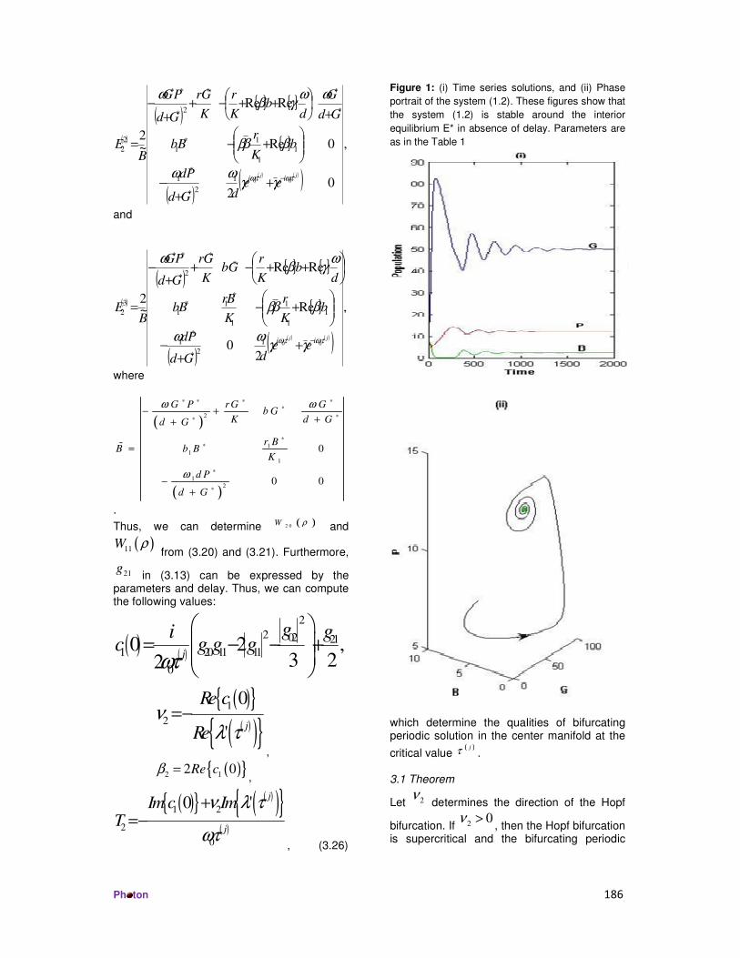
Figure 1: (i) Time series solutions, and (ii) Phase

portrait of the system (1.2). These figures show that

the system (1.2) is stable around the interior

equilibrium E* in absence of delay. Parameters are

as in the Table 1

which determine the qualities of bifurcating periodic solution in the center manifold at the

critical value ( )jτ .

3.1 Theorem

Let 2ν

determines the direction of the Hopf

bifurcation. If 20ν >

, then the Hopf bifurcation is supercritical and the bifurcating periodic

Ph ton 187

solutions exit for ( )jτ τ> . If 2

0ν <, then the

Hopf bifurcation is subcritical and the

bifurcating periodic solutions exit for ( )jτ τ< .

Also 2β determines the stability of the bifurca-

ting periodic solutions: the bifurcating periodic

solutions are stable if 2 0β < and unstable if

20β >

. 2T

determines the period of the bifurcating periodic solutions: the period

increase if 20T >

and decrease if 20T <

. 5. Results and Discussions In this section, we present some numerical simulations to illustrate the analytical results observed in the previous sections. We consider the parameter values as in the Table 1. For this parameter set, the system (1.2) has a unique coexistence equilibrium point

( ) ( )*, , 5 0 , 2 .5 ,1 3 .6 5E G B P∗ ∗ ∗= =

. Fig. 1

shows that the coexistence equilibrium *E is

locally asymptotically stable when 0τ = . In presence of delay, the parameter set also satisfies conditions of the Theorem (i). One

can calculate that 00.0279ω =

, 07.1708τ =

and

( )' 0 . 0 2 7k

g h = > 0. In this case, the

coexistence equilibrium point *E remains

stable for 0[0, )τ τ∈

and unstable for 0τ τ>

. The system (1.2) undergoes a Hopf bifurcation

at *E when 0

7.1708τ τ= =, following the

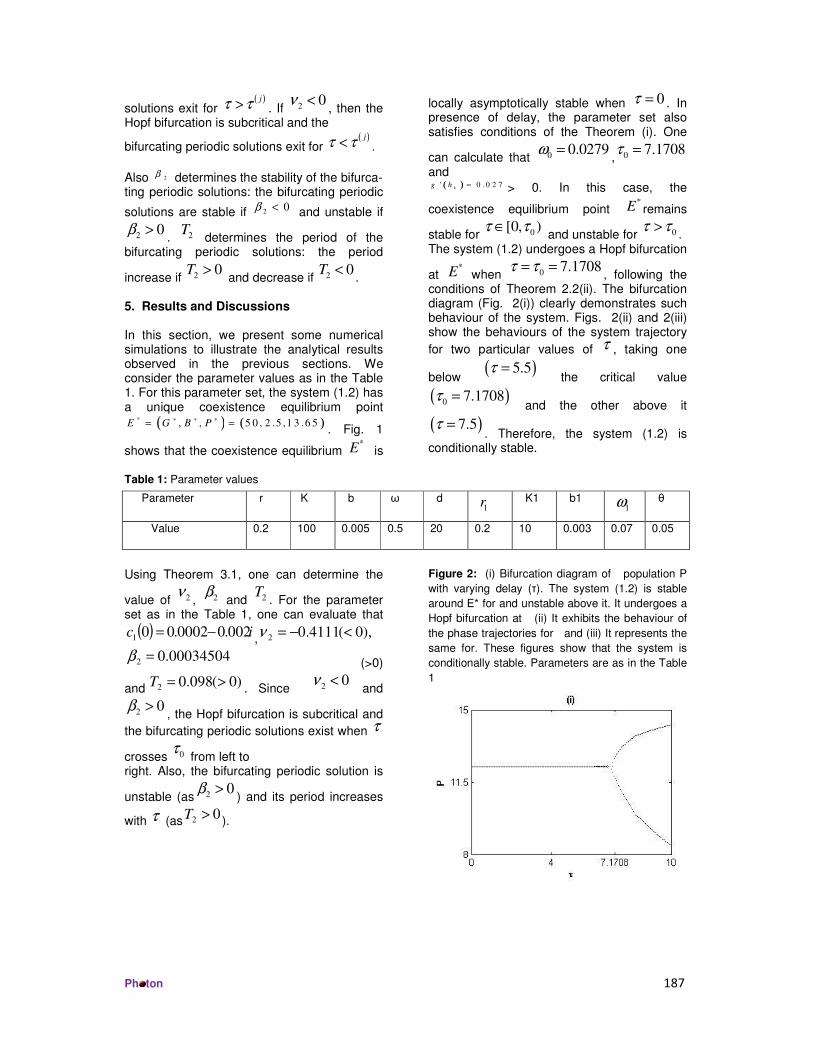
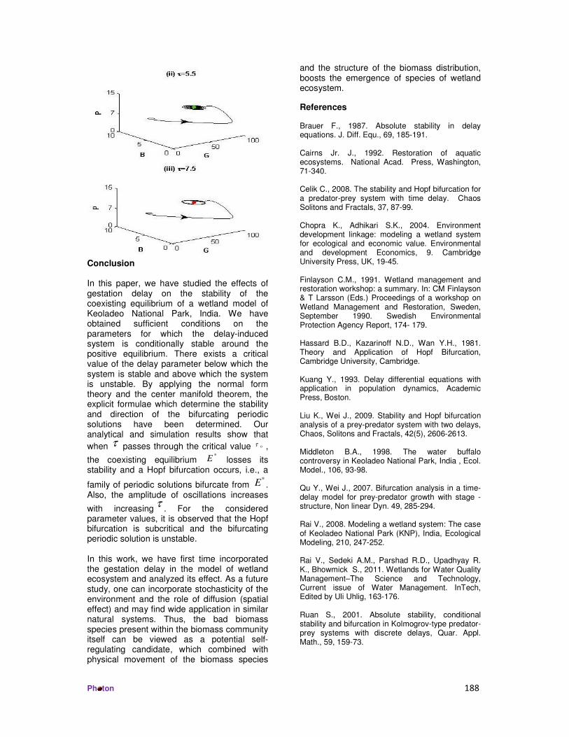
conditions of Theorem 2.2(ii). The bifurcation diagram (Fig. 2(i)) clearly demonstrates such behaviour of the system. Figs. 2(ii) and 2(iii) show the behaviours of the system trajectory

for two particular values of τ , taking one

below ( )5.5τ =

the critical value

( )07.1708τ =

and the other above it

( )7.5τ =. Therefore, the system (1.2) is

conditionally stable.

Table 1: Parameter values

Using Theorem 3.1, one can determine the

value of 2ν

, 2β

and 2T

. For the parameter set as in the Table 1, one can evaluate that

( ) ic 002.00002.001 −=,

),0(4111.02 <−=ν

00034504.02 =β (>0)

and)0(098.02 >=T

. Since 20ν <

and

20β >

, the Hopf bifurcation is subcritical and

the bifurcating periodic solutions exist when τ

crosses 0τ

from left to right. Also, the bifurcating periodic solution is

unstable (as 20β >

) and its period increases

with τ (as02 >T

).

Figure 2: (i) Bifurcation diagram of population P

with varying delay (τ). The system (1.2) is stable

around E* for and unstable above it. It undergoes a

Hopf bifurcation at (ii) It exhibits the behaviour of

the phase trajectories for and (iii) It represents the

same for. These figures show that the system is

conditionally stable. Parameters are as in the Table

1

Parameter

r K b ω d 1r

K1 b1

1ω

θ

Value 0.2 100 0.005 0.5 20 0.2 10 0.003 0.07 0.05

Ph ton 188

Conclusion In this paper, we have studied the effects of gestation delay on the stability of the coexisting equilibrium of a wetland model of Keoladeo National Park, India. We have obtained sufficient conditions on the parameters for which the delay-induced system is conditionally stable around the positive equilibrium. There exists a critical value of the delay parameter below which the system is stable and above which the system is unstable. By applying the normal form theory and the center manifold theorem, the explicit formulae which determine the stability and direction of the bifurcating periodic solutions have been determined. Our analytical and simulation results show that

when τ passes through the critical value 0τ ,

the coexisting equilibrium *E losses its

stability and a Hopf bifurcation occurs, i.e., a

family of periodic solutions bifurcate from *E .

Also, the amplitude of oscillations increases

with increasingτ

. For the considered parameter values, it is observed that the Hopf bifurcation is subcritical and the bifurcating periodic solution is unstable. In this work, we have first time incorporated the gestation delay in the model of wetland ecosystem and analyzed its effect. As a future study, one can incorporate stochasticity of the environment and the role of diffusion (spatial effect) and may find wide application in similar natural systems. Thus, the bad biomass species present within the biomass community itself can be viewed as a potential self-regulating candidate, which combined with physical movement of the biomass species

and the structure of the biomass distribution, boosts the emergence of species of wetland ecosystem.

References Brauer F., 1987. Absolute stability in delay equations. J. Diff. Equ., 69, 185-191. Cairns Jr. J., 1992. Restoration of aquatic ecosystems. National Acad. Press, Washington, 71-340. Celik C., 2008. The stability and Hopf bifurcation for a predator-prey system with time delay. Chaos Solitons and Fractals, 37, 87-99. Chopra K., Adhikari S.K., 2004. Environment development linkage: modeling a wetland system for ecological and economic value. Environmental and development Economics, 9. Cambridge University Press, UK, 19-45. Finlayson C.M., 1991. Wetland management and restoration workshop: a summary. In: CM Finlayson & T Larsson (Eds.) Proceedings of a workshop on Wetland Management and Restoration, Sweden, September 1990. Swedish Environmental Protection Agency Report, 174- 179. Hassard B.D., Kazarinoff N.D., Wan Y.H., 1981. Theory and Application of Hopf Bifurcation, Cambridge University, Cambridge. Kuang Y., 1993. Delay differential equations with application in population dynamics, Academic Press, Boston. Liu K., Wei J., 2009. Stability and Hopf bifurcation analysis of a prey-predator system with two delays, Chaos, Solitons and Fractals, 42(5), 2606-2613. Middleton B.A., 1998. The water buffalo controversy in Keoladeo National Park, India , Ecol. Model., 106, 93-98. Qu Y., Wei J., 2007. Bifurcation analysis in a time-delay model for prey-predator growth with stage -structure, Non linear Dyn. 49, 285-294. Rai V., 2008. Modeling a wetland system: The case of Keoladeo National Park (KNP), India, Ecological Modeling, 210, 247-252. Rai V., Sedeki A.M., Parshad R.D., Upadhyay R. K., Bhowmick S., 2011. Wetlands for Water Quality Management–The Science and Technology, Current issue of Water Management. InTech, Edited by Uli Uhlig, 163-176. Ruan S., 2001. Absolute stability, conditional stability and bifurcation in Kolmogrov-type predator-prey systems with discrete delays, Quar. Appl. Math., 59, 159-73.

Ph ton 189

Ruan S., Wei J., 2001. On the zeros of a third degree exponential polynomial with applications to a delayed model for the control of testosterone secretion, IMA J. Applied Mathematics in Medicine and Biology, 18, 41-52. Ruan S., 2009. On Non-linear Dynamics of Predator - Prey Models with Discrete Delay, Math. Model. Nat. Phenom., 4(2), 140-188. Shukla J.B., Dubey B., 1996. Effects of changing habitats on species: application to KNP, India, Ecological Modeling, 86, 91-99. Shukla V.P., 1998. Modeling the dynamics of wetland macro-phytes, KNP, India, Ecol. Model., 109, 99-112. Srinivasu, P.D.N., Chopra K., 2004. The role of systems modelling in policy: A study of Keoladeo National Park (KNP) India, Work- shop - follow - up of the First School on Ecological Economics, March 22-26th, ICTP, Trieste, Italy. Vijayan V.S., 1991. Keoladeo National Park Ecology Study 1980-1990, Final Report Bombay Natural History Society, India (BNHS), Bombay. Wen X., Wang Z., 2002. The existence of periodic solutions for some models with delays, Nonlinear Anal RWA, 3, 567-81. Yang H., Tian Y., 2005. Hopf bifurcation in REM algorithm with communication delay, Chaos, Solitons and Fractals, 25, 1093-1105.