HAL Id: tel-00991706https://tel.archives-ouvertes.fr/tel-00991706

Submitted on 16 May 2014

HAL is a multi-disciplinary open accessarchive for the deposit and dissemination of sci-entific research documents, whether they are pub-lished or not. The documents may come fromteaching and research institutions in France orabroad, or from public or private research centers.

L’archive ouverte pluridisciplinaire HAL, estdestinée au dépôt et à la diffusion de documentsscientifiques de niveau recherche, publiés ou non,émanant des établissements d’enseignement et derecherche français ou étrangers, des laboratoirespublics ou privés.

Modelling ultrafast exciton transfer in fluorene-basedorganic semiconductors

Jean-Christophe Denis

To cite this version:Jean-Christophe Denis. Modelling ultrafast exciton transfer in fluorene-based organic semiconduc-tors. Materials Science [cond-mat.mtrl-sci]. Heriot Watt University, Edinburgh, 2013. English. tel-00991706

MODELLING ULTRAFAST EXCITON TRANSFER IN

FLUORENE-BASED ORGANIC SEMICONDUCTORS

Jean-Christophe H Denis

Submitted for the Degree of Doctor of Philosophy

Heriot-Watt University

School of Engineering and Physical Sciences

Edinburgh, May 2014.

Thesis defended the 3rd of December 2013. Examiners: Jenny Nelson (Imperial

College, London) and David Townsend (Heriot-Watt University, Edinburgh).

The copyright in this thesis is owned by the author. Any quotation from the

thesis or use of any of the information contained in it must acknowledge this thesis

as the source of the quotation or information.

Abstract

We present a theoretical study of exciton dynamics in solutions and films of

fluorene-based molecules, complemented by experimental work carried out by our

colleagues at the University of St Andrews. We start by introducing the importance

and relevance of such a study, and the methods we use to model ultra-fast (pico-

and sub-picosecond) exciton photo-physics in these systems. We then demonstrate

that exciton transfer in solution of some branched star-shaped oligofluorene-based

molecules arises from molecular geometry relaxation, and, at a slower time-scale,

from Forster hopping between the arms. Straight oligofluorenes do not exhibit

ultra-fast exciton transfer in solution. Finally, we introduce improvements to the

standard line-dipole theory which we use to build a microscopic model for ultra-fast

exciton dynamics in polyfluorene films. Our results show very good agreement with

experiments and enable us to gain fundamental insight into the exciton transfer

processes in these materials.

ii

Acknowledgements

I must say I would never have been able to achieve the work presented here

without the help, support and company of quite a few people around me.

First of all, I would like to express my gratitude and sincerest thanks to my

supervisor, Prof. Ian Galbraith. His continuous support, ideas, comments, patience

and help during these four years have resulted in an efficient and successful super-

vision, which led to the work I present here.

Dr. Stefan Schumacher has played a major role as well in the work presented in

this thesis, thanks to his patience, support and numerous inspirational discussions

and ideas. The three visits I made to Paderborn, in addition to being very useful and

productive, were also very enjoyable thanks to him, his colleagues and his family.

Thank you all very much!

I also address my gratitude to the experimental team in St Andrews for all the

time we spent together trying to understand the work we were respectively doing,

and how to successfully combine theory and experiments to make stronger science.

Thanks to you, Dr. Neil Montgomery, Dr. Gordon Hedley, Dr. Arvydas Ruseckas,

Alex Ward, Dr. Graham Turnbull and Prof. Ifor Samuel, our collaboration was very

fruitful and resulted into more relevant and deeper research.

I must thank Dr Martin Paterson too for his helpful discussions regarding quan-

tum chemistry and theoretical chemistry.

Additional warm thanks go to my colleagues Peter, Natalia, Matthew and Se-

bastian, for the enjoyable lunches and breaks we had together, which made daily

PhD-life much more pleasant. Thanks for the good times, guys!

I must also thank my Best Friend, Bryony, for having proofread my thesis and for

her help with my sometimes incorrect English. Thank you for your great friendship

and your prompt useful work, at sometimes short notice - I will be there for you

when needed.

Finally, a number of friends and relatives have helped me making this long and

difficult journey easier. In particular, I would like to address special thanks to my

parents, grand parents, brother and my local Edinburgh “family” who all made my

daily life better and gave me the strength and motivation I needed: Abdelhamid,

Bryony and Jenny. I am very lucky to have you; without you, I could not have done

this.

iii

List of publications

Part of the work presented in this thesis has been published in the

form of journal articles.

• N. A. Montgomery, J.C. Denis, S. Schumacher, A. Ruseckas, P. J. Skabara,

A. Kanibolotsky, M. J. Paterson, I. Galbraith, G. A. Turnbull, and I. D. W.

Samuel. Optical Excitations in Star-Shaped Fluorene Molecules. The Journal

of Physical Chemistry A 115 (14), 29132919 (2011)

This article corresponds to the work presented in Chapter 3.

• N. A. Montgomery, G. Hedley, A. Ruseckas, J.C. Denis, S. Schumacher, A.

L. Kanibolotsky, P. J. Skabara, I. Galbraith, G. A. Turnbull, and I. D. W.

Samuel. Dynamics of fluorescence depolarization in branched oligofluorene-

truxene molecules. Physical Chemistry Chemical Physics 14, 9176 (2012)

Some of the results described in Chapter 4 have been presented in

this article.

• J.C. Denis, S. Schumacher, and I. Galbraith. Quantitative description of

inter-actions between linear organic chromophores. The Journal of Chemi-

cal Physics 137(22), 224102 (2012)

The results presented in this article constitute Chapter 5.

iv

Contents

Abstract ii

Acknowledgements iii

List of publications iv

1 Introduction 1

1.1 Organic semiconductors: Background . . . . . . . . . . . . . . . . . . 1

1.1.1 A short history . . . . . . . . . . . . . . . . . . . . . . . . . . 1

1.1.2 Basic photo-physics of organic semiconductors . . . . . . . . . 2

1.2 Ultrafast photo-physics in organic semiconductors . . . . . . . . . . . 4

1.2.1 Photo-excitation of a single molecule: simple picture . . . . . 4

1.2.2 Molecular vibrations: Impact on photophysics . . . . . . . . . 7

1.2.3 Multiple chromophores: Exciton transfer . . . . . . . . . . . . 7

1.2.4 Forster theory: Incoherent exciton transfer . . . . . . . . . . 10

1.2.5 Dexter theory: Incoherent exciton transfer . . . . . . . . . . . 12

1.2.6 Beyond Forster-Dexter theory: Incoherent exciton transfer . . 14

1.2.7 Coherent exciton transfer . . . . . . . . . . . . . . . . . . . . 15

1.2.8 Partially-coherent exciton transfer . . . . . . . . . . . . . . . . 16

1.3 Principles of the operation of organic semiconducting devices . . . . . 16

1.3.1 Lasers . . . . . . . . . . . . . . . . . . . . . . . . . . . . . . . 16

1.3.2 Photovoltaic cells . . . . . . . . . . . . . . . . . . . . . . . . . 19

1.3.3 Organic light emitting diodes (OLEDs) . . . . . . . . . . . . . 22

1.4 Current challenges . . . . . . . . . . . . . . . . . . . . . . . . . . . . 24

1.5 Aim of the thesis . . . . . . . . . . . . . . . . . . . . . . . . . . . . . 26

2 Methods 27

2.1 Introduction . . . . . . . . . . . . . . . . . . . . . . . . . . . . . . . . 27

2.2 Quantum chemistry . . . . . . . . . . . . . . . . . . . . . . . . . . . . 28

2.2.1 Large-scale atomistic systems methods . . . . . . . . . . . . . 28

2.2.2 Small-scale atomistic systems methods . . . . . . . . . . . . . 28

2.3 QC: Electronic structure methods . . . . . . . . . . . . . . . . . . . . 29

2.3.1 Background . . . . . . . . . . . . . . . . . . . . . . . . . . . . 29

2.3.2 DFT: Choice of functional and basis-sets . . . . . . . . . . . . 34

2.3.3 Calculation scheme . . . . . . . . . . . . . . . . . . . . . . . . 36

2.4 Bloch equations . . . . . . . . . . . . . . . . . . . . . . . . . . . . . . 41

v

2.4.1 Background . . . . . . . . . . . . . . . . . . . . . . . . . . . . 41

2.4.2 Application for the photo-physics of organic semiconductors . 42

2.4.3 Preliminary results . . . . . . . . . . . . . . . . . . . . . . . . 42

2.4.4 Limitations of this approach . . . . . . . . . . . . . . . . . . . 55

2.5 Conclusion . . . . . . . . . . . . . . . . . . . . . . . . . . . . . . . . . 56

3 Optical properties of fluorene-based C3-symmetric molecules 57

3.1 Background: why are star-shaped molecules important? . . . . . . . . 57

3.2 Methods for the optical and electronic studies of star-shaped molecules 59

3.2.1 Quantum chemistry calculations: methods . . . . . . . . . . . 59

3.2.2 Experimental methods . . . . . . . . . . . . . . . . . . . . . . 61

3.3 Comparison between theoretical and experimental results . . . . . . . 62

3.4 Exciton localisation and symmetry breaking . . . . . . . . . . . . . . 67

3.5 Conclusion . . . . . . . . . . . . . . . . . . . . . . . . . . . . . . . . . 70

4 Intra-molecular exciton transfer in C3-symmetric molecules 72

4.1 Background . . . . . . . . . . . . . . . . . . . . . . . . . . . . . . . . 72

4.2 Fluorescence anisotropy theory . . . . . . . . . . . . . . . . . . . . . 73

4.2.1 Background to fluorescence anisotropy . . . . . . . . . . . . . 73

4.2.2 Fluorescence anisotropy theory for “rod-like” molecules . . . . 74

4.2.3 Fluorescence anisotropy theory for star-shaped molecules . . . 75

4.3 Comparison with experimental results . . . . . . . . . . . . . . . . . . 78

4.3.1 Experimental methods . . . . . . . . . . . . . . . . . . . . . . 79

4.3.2 Experimental results . . . . . . . . . . . . . . . . . . . . . . . 80

4.4 Proposed theory I: two-step exciton transfer in “disk-like” molecules . 84

4.4.1 Method . . . . . . . . . . . . . . . . . . . . . . . . . . . . . . 84

4.4.2 Results . . . . . . . . . . . . . . . . . . . . . . . . . . . . . . . 86

4.5 Proposed theory II: influence of symmetry-breaking defects . . . . . . 87

4.5.1 Method . . . . . . . . . . . . . . . . . . . . . . . . . . . . . . 87

4.5.2 Fast depolarisation component . . . . . . . . . . . . . . . . . . 88

4.5.3 Slower depolarisation component . . . . . . . . . . . . . . . . 92

4.6 Assignment of depolarisation processes . . . . . . . . . . . . . . . . . 93

4.7 Conclusion . . . . . . . . . . . . . . . . . . . . . . . . . . . . . . . . . 94

5 Dipole approximations to calculate intermolecular interactions 96

5.1 Introduction . . . . . . . . . . . . . . . . . . . . . . . . . . . . . . . . 96

5.2 Background: dipole models . . . . . . . . . . . . . . . . . . . . . . . . 97

5.3 Method: calculation of interaction energies by quantum chemistry . . 99

5.4 Results and discussion . . . . . . . . . . . . . . . . . . . . . . . . . . 101

5.4.1 Short molecules – the O2 dimer . . . . . . . . . . . . . . . . . 102

vi

5.4.2 Long molecules – the O8 octamer . . . . . . . . . . . . . . . . 103

5.5 An improved line-dipole approximation . . . . . . . . . . . . . . . . . 107

5.6 Conclusion . . . . . . . . . . . . . . . . . . . . . . . . . . . . . . . . . 111

6 A microscopic model of exciton dynamics in polyfluorene films 113

6.1 Introduction . . . . . . . . . . . . . . . . . . . . . . . . . . . . . . . . 113

6.2 Experiments: fluorescence anisotropy in PFO films . . . . . . . . . . 114

6.2.1 Experimental methodology . . . . . . . . . . . . . . . . . . . . 114

6.2.2 Experimental results . . . . . . . . . . . . . . . . . . . . . . . 115

6.2.3 Macroscopic description . . . . . . . . . . . . . . . . . . . . . 117

6.3 Microscopic theory of exciton diffusion in PFO films . . . . . . . . . . 119

6.3.1 The microscopic model . . . . . . . . . . . . . . . . . . . . . . 119

6.3.2 Exciton dynamics . . . . . . . . . . . . . . . . . . . . . . . . . 121

6.3.3 Fluorescence anisotropy . . . . . . . . . . . . . . . . . . . . . 124

6.4 Parameter selection - low pump intensity . . . . . . . . . . . . . . . . 124

6.4.1 Geometrical parameters . . . . . . . . . . . . . . . . . . . . . 125

6.4.2 Spectral Parameters . . . . . . . . . . . . . . . . . . . . . . . 126

6.5 Results and discussion: low pump intensity . . . . . . . . . . . . . . 128

6.5.1 Fluorescence anisotropy . . . . . . . . . . . . . . . . . . . . . 128

6.5.2 Insights into spectral and spatial energy migration . . . . . . . 128

6.5.3 Exciton diffusion length . . . . . . . . . . . . . . . . . . . . . 135

6.6 High pump intensity: exciton-exciton annihilation . . . . . . . . . . . 137

6.6.1 Excited-state absorption parameter selection . . . . . . . . . . 138

6.6.2 Results and discussion . . . . . . . . . . . . . . . . . . . . . . 140

6.7 Conclusions . . . . . . . . . . . . . . . . . . . . . . . . . . . . . . . . 143

7 Conclusions and future work 144

7.1 Conclusions . . . . . . . . . . . . . . . . . . . . . . . . . . . . . . . . 144

7.2 Future work . . . . . . . . . . . . . . . . . . . . . . . . . . . . . . . . 147

Appendix A 149

A.1 Spectral overlaps between two chromophores . . . . . . . . . . . . . . 149

A.2 Derivation of the source term . . . . . . . . . . . . . . . . . . . . . . 149

References 151

vii

Chapter 1

Introduction

This thesis is focused on ultra-fast (pico- and sub-picosecond) exciton transfer

in polyfluorene-based organic semiconductors. In this introduction we will define

what organic semiconductors are and highlight some of their key properties, before

focusing on the ultra-fast photo-physics of these materials. We will then motivate

the importance of understanding the fundamental physics of these materials through

a study of their applications in devices, and highlight the current research challenges

that these material are facing.

1.1 Organic semiconductors: Background

“Organic semiconductors”, or “molecular semiconductors”, are materials which,

like any semiconductor, do not conduct charges as much as a metals do, but do

conduct better than isolators. They are molecular materials made of organic com-

pounds, whereas “inorganic semiconductors” are crystals made of elements from the

columns II to VI in the periodic table of elements [1]. A more rigorous definition,

as well as detailed basic physics principles, will be provided in Section 1.1.2.

1.1.1 A short history

Organic semiconductors emerged much later than their inorganic counterparts.

Indeed, the first report of highly conductive polymers was made in 1963 [2], whereas

the first inorganic semiconductor diode laser (made of gallium-arsenide) had al-

ready been created three years earlier [3]. Organic semiconductor devices therefore

appeared long after their inorganic equivalents: whereas an inorganic light emitting

diode (LED) was realised for the first time in 1962 [4], the first demonstration of an

organic LED (OLED) dates from 1987 [5]. Similarly, organic transistors were first

developed in 1986 [6], much later than the realisation of the first inorganic transistor

created in 1947 [7]. This is true for photovoltaic cells as well: the first silicon solar

cell was produced in 1954, with an efficiency of 6% [8]; in contrast, the first organic

cell, with an efficiency of around 1%, was created in 1986 [9]. However organic

lasers appeared quite early, in 1967, in the form of dye lasers, usually consisting of

crystals of dye-doped polymer [10, 11], and even made a significant contribution to

the development of both organic and inorganic lasers [12]. Non-dye based, organic

semiconductor lasers appeared in 1992 [13].

1

The much more recent discovery and investigation of organic semiconductors,

compared to the longer history of inorganic semiconductors, is one of the main

reasons why organic semiconducting devices are not widely commercially available.

However, they are the subject of important research efforts due to their advantages

over inorganic semiconductors, and therefore their potential to replace them in the

near future, as we shall see in the rest of this introduction.

1.1.2 Basic photo-physics of organic semiconductors

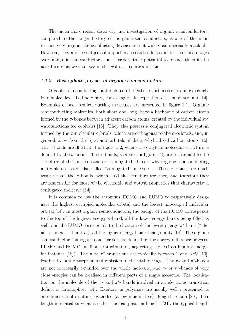
Organic semiconducting materials can be either short molecules or extremely

long molecules called polymers, consisting of the repetition of a monomer unit [14].

Examples of such semiconducting molecules are presented in figure 1.1. Organic

semiconducting molecules, both short and long, have a backbone of carbon atoms

formed by the σ-bonds between adjacent carbon atoms, created by the individual sp2

wavefunctions (or orbitals) [15]. They also possess a conjugated electronic system

formed by the π-molecular orbitals, which are orthogonal to the σ-orbitals, and, in

general, arise from the pz atomic orbitals of the sp2-hybridized carbon atoms [16].

These bonds are illustrated in figure 1.2, where the ethylene molecular structure is

defined by the σ-bonds. The π-bonds, sketched in figure 1.2, are orthogonal to the

structure of the molecule and are conjugated. This is why organic semiconducting

materials are often also called “conjugated molecules”. These π-bonds are much

weaker than the σ-bonds, which hold the structure together, and therefore they

are responsible for most of the electronic and optical properties that characterise a

conjugated molecule [14].

It is common to use the acronyms HOMO and LUMO to respectively desig-

nate the highest occupied molecular orbital and the lowest unoccupied molecular

orbital [14]. In most organic semiconductors, the energy of the HOMO corresponds

to the top of the highest energy π-band, all the lower energy bands being filled as

well, and the LUMO corresponds to the bottom of the lowest energy π∗-band (∗ de-

notes an excited orbital), all the higher energy bands being empty [14]. The organic

semiconductor “bandgap” can therefore be defined by the energy difference between

LUMO and HOMO (at first approximation, neglecting the exciton binding energy,

for instance [18]). The π to π∗ transitions are typically between 1 and 3 eV [19],

leading to light absorption and emission in the visible range. The π- and π∗-bands

are not necessarily extended over the whole molecule, and π- or π∗-bands of very

close energies can be localised in different parts of a single molecule. The localisa-

tion on the molecule of the π- and π∗- bands involved in an electronic transition

defines a chromophore [14]. Excitons in polymers are usually well represented as

one dimensional excitons, extended (a few nanometres) along the chain [20]; their

length is related to what is called the “conjugation length” [21], the typical length

2

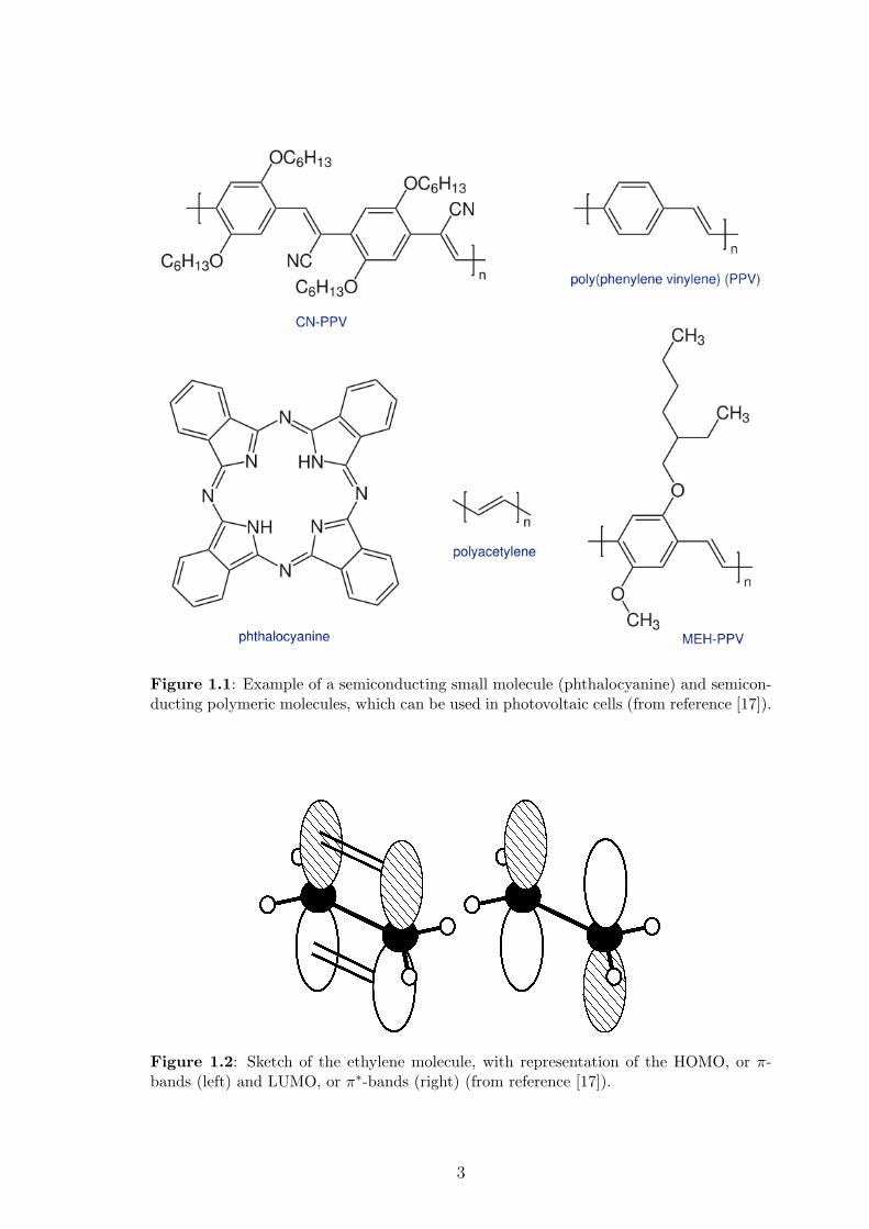
Figure 1.1: Example of a semiconducting small molecule (phthalocyanine) and semicon-ducting polymeric molecules, which can be used in photovoltaic cells (from reference [17]).

Figure 1.2: Sketch of the ethylene molecule, with representation of the HOMO, or π-bands (left) and LUMO, or π∗-bands (right) (from reference [17]).

3

of the polymer chain which is not significantly distorted so that the electronic prop-

erties are the ones of the straight chain. Usually, the definition of a chromophore

is restrained to the transitions in the visible spectra, but we extend it to any tran-

sition in this thesis - by chromophore length we mean the spatial extent of the

polymer where the transition of interest, whatever its energy, takes place. There-

fore, whereas in inorganic semiconductors the bandgap arises from the extended,

ordered lattice [22], in organic semiconductors the bandgap is created and present

in any individual molecule.

Under photo-excitation we can observe photo-conductivity: an electron is pro-

moted from the valence band (π-band) to the conduction band (π∗-band) by photon

absorption [23]. As a result, mobile electrons and holes are created and can move

as a response to an electric field. This property makes organic semiconductors suit-

able for the fabrication of many electronic devices such as light emitters, displays,

transistors, photovoltaic cells and lasers. A detailed study of the photo-physics of

organic semiconductors will be conducted in the next Section, 1.2. We will review

the physics of such devices in Section 1.3.

Semiconducting polymers are stable in a variety of phases, such as gases, so-

lutions or solids (in crystalline, semi-crystalline or amorphous forms), depending

on the molecule and the processing techniques. The main difference between small

molecules and polymers lies in the way they are processed to produce thin-films.

Conjugated polymers need to be spin-coated or deposited by a printing-like tech-

nique, whereas small molecules are deposited onto the film from sublimation or

evaporation, or can also be grown as a single-crystal much more easily than poly-

mers [14].

We will highlight the advantages and drawbacks of organic semiconductors more

specifically in the context of their use in devices in Section 1.3, but one major lim-

itation of most organic semiconducting samples is their poor photo-chemical sta-

bility, particularly when exposed to water, oxygen and modest temperatures [23].

Techniques exist to overcome this limit, such as encapsulation, but could still be im-

proved [24]. One of the main advantages of organic semiconductors is the ease with

which they can be processed, with the possibility of utilising simple “printing tech-

niques” [12]. In contrast, inorganic semiconductors require more complex processing

techniques, such as chemical vapour deposition or molecular beam epitaxy [1].

1.2 Ultrafast photo-physics in organic semiconductors

1.2.1 Photo-excitation of a single molecule: simple picture

Following the absorption of a photon by the semiconducting molecule, an elec-

tron is promoted from the π-band to the π∗-band. A hole is created by the lack of

4

one electron in the HOMO, and this hole is bound to the electron due the attractive

Coulombic force between them. This electron and hole bound state is described by

a quasi-particle, called an “exciton” [25]. Two models exist for the exciton: the

Wannier exciton and the Frenkel exciton [18]. Wannier excitons do not possess

a strongly bound electron and hole (the binding energy is typically less than 0.01

eV [26]), and are therefore delocalised over many atoms, whereas electrons and holes

in the Frenkel model have much stronger binding energies (with values typically re-

ported from 0.4 to 1eV [27–29]). Wannier excitons usually describe excitons in

inorganic semiconductors [23], where the dielectric constant is much higher than in

organic semiconductors. Frenkel excitons usually occur in molecular semiconducting

systems [23]. Therefore, in the rest of this thesis, we will refer to Frenkel excitons

as simply “excitons”.

A chromophore can be, to a certain extent, compared to a harmonic quantum

oscillator; the outcome of this comparison is that the potential energy surface of

the molecule is typically parabolic, as a function of the nuclear coordinates [30] - a

parametrisation of the position of the nuclei of the chromophore. When unexcited,

the chromophore geometry is the ground-state geometry, the ground-state being

denoted in the rest of this thesis as the S0-state. This geometry corresponds to the

minimum of the ground-state potential energy parabola. In the frame of the Born-

Oppenheimer approximation, the nuclei motions are slow compared to the electrons

(see Section 2.3 for more details), and as a consequence the absorption transition

is vertical: the geometry of the chromophore does not undergo any change during

the photon-absorption or emission process. In the rest of this thesis, all transitions

will be vertical: they take place without immediate molecular geometry change, as

sketched in figure 1.3. Just after photo-absorption the chromophore is in the first

excited-state (or any higher excited state, depending on the photon energy), that

we will call in the rest of this thesis the S1-state, and the potential energy surface

of the molecule has changed due to the presence of the excitation, leading to a

different combination of the oscillator modes (see figure 1.3). Due to the coupling

between the chromophore and its environment (solution, phonons), the chromophore

will consequently relax from the S0 geometry to the S1 geometry, corresponding to

the minimum of the S1 potential energy surface. This relaxation is fast, typically

100 fs [31,32]. Radiative decay mechanisms will then be responsible for the emission

of a photon at the emission energy, vertically from the S1 to the S0 potential energy

surface. This will be followed by the relaxation of the molecule from the S1 geometry

back to the ground-state S0 geometry.

This is illustrated in figure 1.3. From this figure it is clear why the absorption

energy is always higher than the emission energy (the difference between the absorp-

tion and emission energies is usually called “Stokes-shift” [14]). For an ensemble of

5

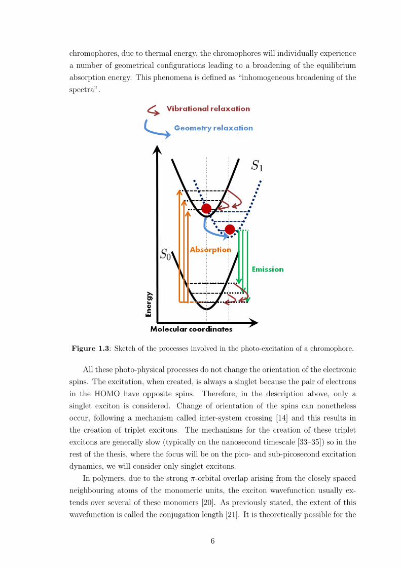
chromophores, due to thermal energy, the chromophores will individually experience

a number of geometrical configurations leading to a broadening of the equilibrium

absorption energy. This phenomena is defined as “inhomogeneous broadening of the

spectra”.

Figure 1.3: Sketch of the processes involved in the photo-excitation of a chromophore.

All these photo-physical processes do not change the orientation of the electronic

spins. The excitation, when created, is always a singlet because the pair of electrons

in the HOMO have opposite spins. Therefore, in the description above, only a

singlet exciton is considered. Change of orientation of the spins can nonetheless

occur, following a mechanism called inter-system crossing [14] and this results in

the creation of triplet excitons. The mechanisms for the creation of these triplet

excitons are generally slow (typically on the nanosecond timescale [33–35]) so in the

rest of the thesis, where the focus will be on the pico- and sub-picosecond excitation

dynamics, we will consider only singlet excitons.

In polymers, due to the strong π-orbital overlap arising from the closely spaced

neighbouring atoms of the monomeric units, the exciton wavefunction usually ex-

tends over several of these monomers [20]. As previously stated, the extent of this

wavefunction is called the conjugation length [21]. It is theoretically possible for the

6

exciton to be extended over chains belonging to neighbouring polymers because of in-

trachain interactions, and the resulting multichain exciton is called an exciplex [36].

However, the significant disorder in polymer films makes this delocalisation very

unlikely; as a result the formation of exciplexes will be ignored in the rest of this

thesis.

Non-radiative decay mechanisms also exist. A measure of the fraction of these

non-radiative decays is given by the photoluminescence quantum yield (PLQY). The

PLQY is defined as the ratio of the number of photons emitted over the number of

photons absorbed [14]. Values range from close to 0% to almost 100% quantum effi-

ciency, meaning that in the latter case almost all excitons follow the recombination

path described above.

1.2.2 Molecular vibrations: Impact on photophysics

A more realistic model includes vibrations; indeed molecules made of hundreds

of atoms possess numerous degrees of freedom, leading to vibrations arising because

of thermal energy and photo-excitation [30]. Due to thermal energy, the energy of

the chromophore will actually not necessarily be the minimum of the ground-state

potential energy surface, but could have a range of values, depending on where the

vibrational modes are energetically situated. The transitions to the excited-state

which will be dominant are the ones reaching a vibrational state of the excited-state

energy potential [30]. Detailed mathematical treatment of the absorption probability

between electronic and vibrational states is given by the Franck-Condon principle,

which is developed in Section 2.4. These vibrations are very evident in the absorption

and emission spectra of a single chromophore, provided the homogeneous linewidth

(the spectral broadening appearing from the dephasing time of the excitation, see

Section 2.4) is not too wide.

1.2.3 Multiple chromophores: Exciton transfer

Once the exciton is created, its transfer to another chromophore is possible. This

transfer can be realised by simple photoluminescence from one chromophore, and re-

absorption of the emitted photon by another chromophore. However, the radiative

lifetimes of the fluorene-bases molecules we investigated in this thesis are longer

than 100 ps [37], whereas we are interested in the picosecond and sub-picosecond

dynamics of such molecules. In the rest of this work, our interest will therefore be

restricted to non-trivial exciton transfer mechanisms, involving no photon-emission

and re-absorption.

We can distinguish two kinds of exciton transfer: either the exciton has reached

a chromophore of the same molecule or it has transferred into the chromophore of an-

7

other molecule. The first case corresponds to “intrachain” exciton transfer whereas

the second case is called “interchain” exciton transfer [38]. Interchain transfer re-

quires close neighbouring molecules and therefore does not take place in well diluted

solutions with small concentrations of organic semiconductors, nor in gas-phases.

Exciton transfer mechanisms lead to the transfer of excitation to low energy

chromophores. This phenomena plays a major role in the ultra-fast photo-physics

processes in organic semiconductors, by governing which subset of chromophores of

the whole ensemble is most likely to become excited after photo-excitation. This

is of crucial importance in devices such as organic light emitting diodes (OLEDs)

and organic photovoltaic cells (OPV), where the the device characteristics are based

on both the photo-physics and charge transport properties (see detailed device de-

scriptions in Section 1.3). It can also lead to the transfer of either the electron or

the hole only, creating a separated electron and hole pair - a quasi-particle which is

known as a “polaron” [36]. However such separation requires one to overcome the

strong exciton binding energy, typically 0.5 eV in polyfluorenes [12], and therefore

requires a specific structure and blend or semiconducting molecular species, as used

in organic photovoltaic cells (see Section 1.3). As we will only study pure-phase

samples of molecules without charge transfer character in this thesis, we will assume

that polaron formation is non-existent at the time-scale we are interested in. This is

also supported by the lack of observed polaron signatures seen during the realisation

of the experiments presented in Chapters 3, 4 and 6.

The need for a theory enabling the excitation transfer in organic materials ap-

peared in the middle of the twentieth century, when it was observed that the PQLY

of dye species were significantly different whether they were in solution or in solid

phase [39, 40]. One of the explanations at this time was that the excitation was

transferred to lower energy molecules in films (in diluted solutions, non-aggregated

molecules behave like isolated molecules), and if these molecules to which the exci-

tation transferred were not fluorescent (dark), this resulted in the observed PLQY

loss [41].

Energy transfer processes are intimately linked to the interactions between chro-

mophores. In the following work, we will present three interaction regimes: the

weak, intermediate and strong coupling regimes. These regimes are determined by

the comparison of two distinct timescales [30]: the vibrational relaxation time τrelax

and the exciton transfer time τtransfer. τrelax is the time it takes for an excited chro-

mophore to return to the thermal equilibrium of the excited-state from the “hot”

out-of equilibrium vibrations induced by the vertical photo-induced electronic tran-

sition. It is intrinsically linked to the decoherence time, because such vibrational

relaxation induces dephasing. Therefore a system with fast relaxation times will

loose its quantum coherence quickly. τtransfer is simply the typical time associated

8

with the movement of one exciton from an excited chromophore to a non-excited

chromophore in the ground-state; it is directly linked with the interaction strength

between these two chromophores, and with their spectral matching. All exciton

transfers arise from the following Hamiltonian [42]:

H = H0 +Hel +Hel−vib , (1.1)

with H0 being:

H0 =∑

n

εn |n〉 〈n|+∑

n,k

~ωn,kb†n,kbn,k , (1.2)

where |n〉 is an excitation created in the n-th chromophore site, εn its associated

energy, ~ωn,k is the energy of the k-th vibrational state of the n-th chromophore,

with b†n,k and bn,k being respectively its bosonic creation and annihilation operator.

Hel describes the intermolecular electronic coupling:

Hel =∑

m>n

∑

n

Jm,n (|n〉 〈m|+ |m〉 〈n|) , (1.3)

with Jm,n being the electronic coupling between chromophores m and n. Hel−bath

represents the electronic interaction with the bath.

Hel−bath =∑

n

∑

k

gn,k

(b†n,k + bn,k

)|n〉 〈n| , (1.4)

where gn,k is the coupling of the k-th vibrational mode of the n-th chromophore

with the phonon bath.

The ratio between the energy difference and the electronic coupling of two chro-

mophores (|εm − εn|/Jm,n) defines the localisation of the excited state [42].

The comparison of the electronic coupling between two chromophores and their

coupling with the phonon bath determines if the transfer is coherent or not. Indeed,

the electronic coupling is linked to the exciton transfer rate τtransfer, whereas the

chromophore-phonon bath coupling relates to τrelax [30].

We can therefore distinguish three cases, depending on the comparison between

these characteristic times [30, 42,43]:

• τrelax ≪ τtransfer, in such a case the exciton transfer take place when the

chromophore is totally relaxed to the excited-state equilibrium geometry, and

therefore the coherences do not exist any more. This case is thus called inco-

herent transfer, or the weak coupling limit.

• τrelax ≫ τtransfer. In this situation, coherence is long lived compared to the

transfer, so the exciton is a quantum mechanical wave packet. It can in conse-

9

quence move almost freely from chromophore to chromophore. Such transfer

is therefore called coherent transfer, or transfer in the strong coupling limit.

• τrelax ≈ τtransfer. This case is not trivial, as the exciton motion is at the

border between coherent and incoherent. Additionally, the definition of such a

system is not straightforward: if the molecular sample is made of aggregates,

it is possible that the exciton motion in an aggregate is coherent, whereas the

motion between aggregates is not. This regime is called partially coherent, or

the intermediate coupling limit.

In particular, the assumption that incoherent transfer is the dominating transfer

mechanism is consistent with the assumption that excitons are localised on one

chromophore - the weak coupling limit. We assume that in fluorene-based molecules,

|εm− εn| ≫ Jm,n, so that the exciton is localised on only one chromophore and that

weak coupling applies. This confirmed by results from Chapters 4 and 6.

The electronic coupling V between the acceptor and donor molecules can be par-

titioned into two coupling mechanisms [43]: one coupling arising from the Coulombic

interaction between the charged particles, VC , and one associated with the degree

of overlap between the molecular orbitals of the donor and acceptor, the exchange-

interaction VX .

V = VC + VX . (1.5)

Two theories have developed to describe incoherent energy transfer, depend-

ing on which coupling energy is dominant. If the coupling energy is dominated by

Coulomb coupling, the associated coupling is called Forster transfer and is based

on resonant, dipole-induced energy transfer. Conversely, if the main coupling mech-

anism is the overlap between molecular orbitals, the transfer is Dexter-type and

relies on electron exchange. Therefore, Forster transfer deals with long-range en-

ergy transfer whereas Dexter transfer deals with short-range energy transfer.

1.2.4 Forster theory: Incoherent exciton transfer

It was first proposed that excitation transfer in organic semiconductors was

similar to energy transfer in coupled oscillators [42]: if one excites a spring which

is weakly coupled to another one, it is possible to see the oscillation spreading and

being transferred to the other coupled spring. In the case of chromophores, the

coupling is between the transition densities of each chromophore. Indeed, if these

charges are spatially distributed so that light interaction with the chromophore is

possible, an oscillating dipole is created on the chromophore, conceptually analogous

to an oscillating spring. In this frame, the coupling energy between chromophores

is therefore approximated as V ≈ VC . Knowing the wavefunction of state i of

10

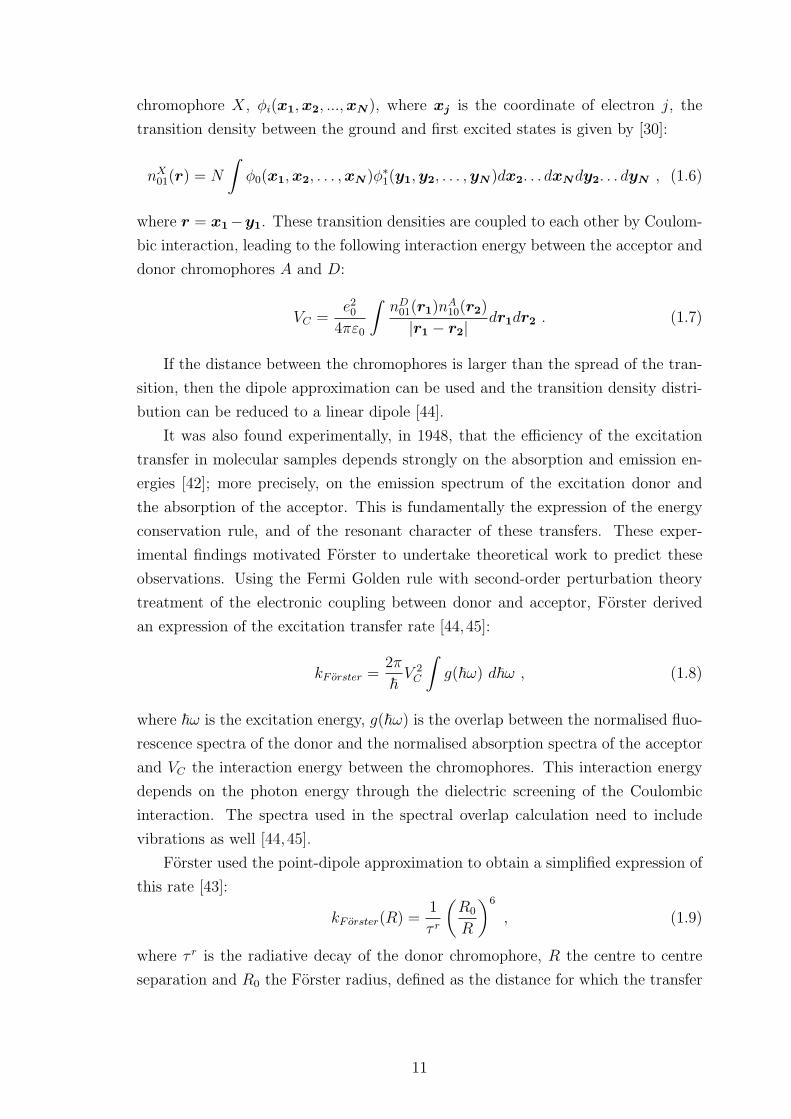
chromophore X, φi(x1,x2, ...,xN ), where xj is the coordinate of electron j, the

transition density between the ground and first excited states is given by [30]:

nX01(r) = N

∫φ0(x1,x2, . . . ,xN )φ∗

1(y1,y2, . . . ,yN )dx2. . . dxNdy2. . . dyN , (1.6)

where r = x1−y1. These transition densities are coupled to each other by Coulom-

bic interaction, leading to the following interaction energy between the acceptor and

donor chromophores A and D:

VC =e20

4πε0

∫nD01(r1)n

A10(r2)

|r1 − r2|dr1dr2 . (1.7)

If the distance between the chromophores is larger than the spread of the tran-

sition, then the dipole approximation can be used and the transition density distri-

bution can be reduced to a linear dipole [44].

It was also found experimentally, in 1948, that the efficiency of the excitation

transfer in molecular samples depends strongly on the absorption and emission en-

ergies [42]; more precisely, on the emission spectrum of the excitation donor and

the absorption of the acceptor. This is fundamentally the expression of the energy

conservation rule, and of the resonant character of these transfers. These exper-

imental findings motivated Forster to undertake theoretical work to predict these

observations. Using the Fermi Golden rule with second-order perturbation theory

treatment of the electronic coupling between donor and acceptor, Forster derived

an expression of the excitation transfer rate [44, 45]:

kF orster =2π

~V 2C

∫g(~ω) d~ω , (1.8)

where ~ω is the excitation energy, g(~ω) is the overlap between the normalised fluo-

rescence spectra of the donor and the normalised absorption spectra of the acceptor

and VC the interaction energy between the chromophores. This interaction energy

depends on the photon energy through the dielectric screening of the Coulombic

interaction. The spectra used in the spectral overlap calculation need to include

vibrations as well [44, 45].

Forster used the point-dipole approximation to obtain a simplified expression of

this rate [43]:

kF orster(R) =1

τ r

(R0

R

)6

, (1.9)

where τ r is the radiative decay of the donor chromophore, R the centre to centre

separation and R0 the Forster radius, defined as the distance for which the transfer

11

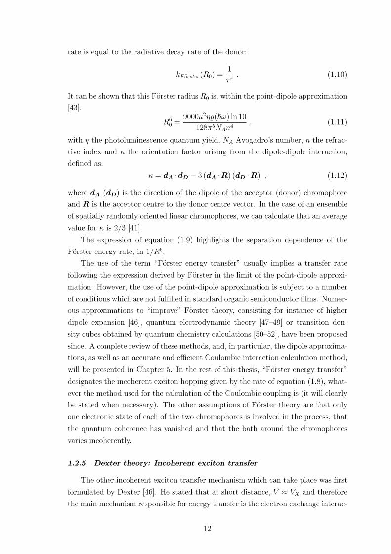
rate is equal to the radiative decay rate of the donor:

kF orster(R0) =1

τ r. (1.10)

It can be shown that this Forster radius R0 is, within the point-dipole approximation

[43]:

R60 =

9000κ2ηg(~ω) ln 10

128π5NAn4, (1.11)

with η the photoluminescence quantum yield, NA Avogadro’s number, n the refrac-

tive index and κ the orientation factor arising from the dipole-dipole interaction,

defined as:

κ = dA ·dD − 3 (dA ·R) (dD ·R) , (1.12)

where dA (dD) is the direction of the dipole of the acceptor (donor) chromophore

and R is the acceptor centre to the donor centre vector. In the case of an ensemble

of spatially randomly oriented linear chromophores, we can calculate that an average

value for κ is 2/3 [41].

The expression of equation (1.9) highlights the separation dependence of the

Forster energy rate, in 1/R6.

The use of the term “Forster energy transfer” usually implies a transfer rate

following the expression derived by Forster in the limit of the point-dipole approxi-

mation. However, the use of the point-dipole approximation is subject to a number

of conditions which are not fulfilled in standard organic semiconductor films. Numer-

ous approximations to “improve” Forster theory, consisting for instance of higher

dipole expansion [46], quantum electrodynamic theory [47–49] or transition den-

sity cubes obtained by quantum chemistry calculations [50–52], have been proposed

since. A complete review of these methods, and, in particular, the dipole approxima-

tions, as well as an accurate and efficient Coulombic interaction calculation method,

will be presented in Chapter 5. In the rest of this thesis, “Forster energy transfer”

designates the incoherent exciton hopping given by the rate of equation (1.8), what-

ever the method used for the calculation of the Coulombic coupling is (it will clearly

be stated when necessary). The other assumptions of Forster theory are that only

one electronic state of each of the two chromophores is involved in the process, that

the quantum coherence has vanished and that the bath around the chromophores

varies incoherently.

1.2.5 Dexter theory: Incoherent exciton transfer

The other incoherent exciton transfer mechanism which can take place was first

formulated by Dexter [46]. He stated that at short distance, V ≈ VX and therefore

the main mechanism responsible for energy transfer is the electron exchange interac-

12

tion. This interaction arises from the symmetrisation of the electronic wavefunctions.

In consequence, if two molecular species are very closely separated, their molecular

orbitals can overlap, leading to electron transfer from the donor to the acceptor.

Dexter stated that, as the molecular orbital tails decay exponentially (typically,

the tail T is proportional to exp(−αR), α being in the range of 1.2-2.0A−1) [42],

therefore the electronic coupling VX varies as VX ∝ exp(−2αR), R being the centre-

to-centre separation of the molecular orbitals [53]. The Dexter electron transfer rate

is the same as for the Forster exciton transfer rate (it depends on the overlap of the

absorption spectra of the acceptor with the fluorescence spectra of the donor, and

on the square of this interaction energy), but the interaction energy is now derived

from the molecular orbital overlap [46]:

kDexter =2π

~V 2X

∫g(~ω)d~ω . (1.13)

This interaction is quite weak compared to the dipole-dipole interaction, except

at short distances, typically for separations less than 5A, where Dexter transfer

dominates [42].

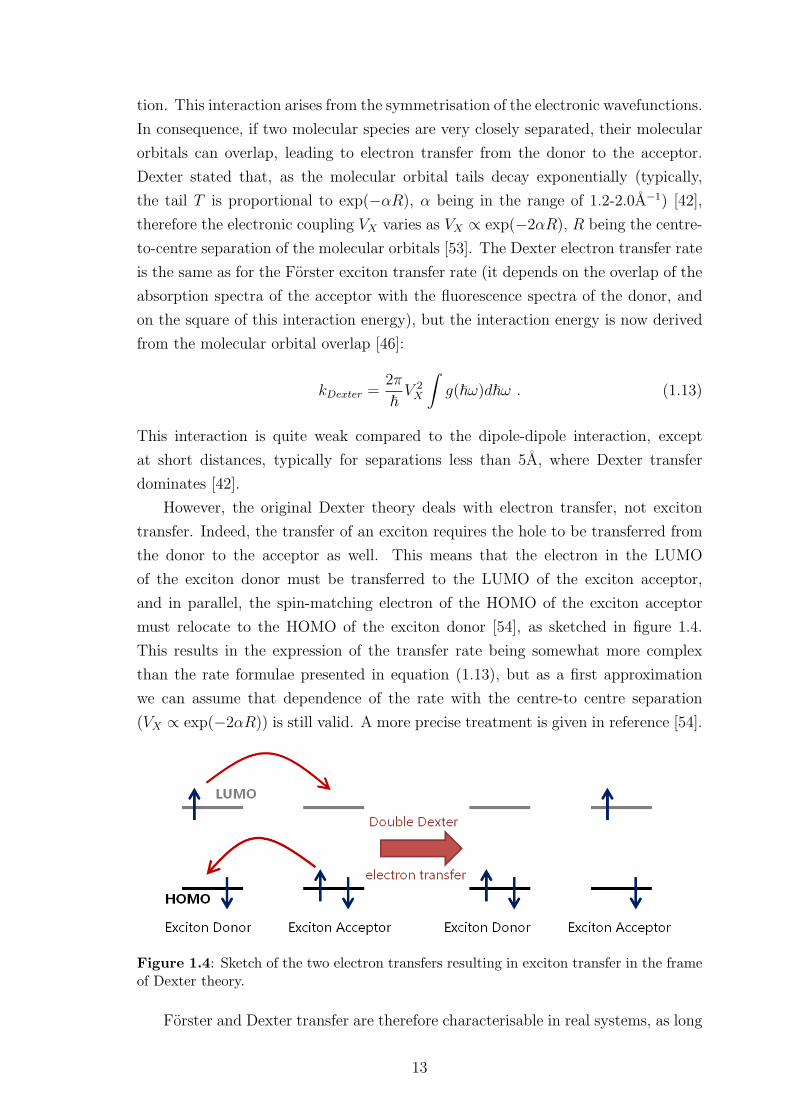
However, the original Dexter theory deals with electron transfer, not exciton

transfer. Indeed, the transfer of an exciton requires the hole to be transferred from

the donor to the acceptor as well. This means that the electron in the LUMO

of the exciton donor must be transferred to the LUMO of the exciton acceptor,

and in parallel, the spin-matching electron of the HOMO of the exciton acceptor

must relocate to the HOMO of the exciton donor [54], as sketched in figure 1.4.

This results in the expression of the transfer rate being somewhat more complex

than the rate formulae presented in equation (1.13), but as a first approximation

we can assume that dependence of the rate with the centre-to centre separation

(VX ∝ exp(−2αR)) is still valid. A more precise treatment is given in reference [54].

Figure 1.4: Sketch of the two electron transfers resulting in exciton transfer in the frameof Dexter theory.

Forster and Dexter transfer are therefore characterisable in real systems, as long

13

as we can measure the distance dependence of the exciton transfers. Indeed, we have

shown that Forster transfer varies approximately in 1/R6, whereas Dexter transfer

varies as exp(−2αR). In theory molecular systems can exhibit both behaviours [42],

depending on how close the chromophores are, and how they are arranged. In the

rest of this thesis, we however exclude Dexter transfer, as we believe fluorene based-

chromophores are not so closely packed that they are within the range of application

of Dexter transfer. Indeed, we show evidence in this thesis that Dexter theory is

not necessary to model exciton transfer in solutions of fluorene-based star-shaped

molecules (Chapter 4) and in polyfluorene films (Chapter 6).

1.2.6 Beyond Forster-Dexter theory: Incoherent exciton transfer

Recent corrections have been proposed to the original incoherent Forster-Dexter

energy transfer theories. Forster based his theory on the Coulombic effect, neglecting

the magnetic effects arising from the magnetic field associated with any electric field.

In most cases, this magnetic field is negligible; however when inter-chromophore

distances are comparable with the excitation wavelength 2πc/ω, where c is the

speed of light and ω the angular frequency of the excitation exchanged between

the chromophores, the full electromagnetic coupling should be taken into account,

and not only the Coulombic coupling [47, 55]. However, due the conditions on the

virtual photon exchanged and the distance between the two involved chromophores

(the wavelength of the photon has to be typically a few nanometers), this applies

only for high energy photons, such as photons in the ultraviolet range [54], and is

mostly relevant for biological systems exposed to such radiations, such as nucleic

acids in DNA [56]. As the fluorene-based molecules we present in the rest of this

thesis emit in the visible spectra, we will be not using this correction to the Forster

theory in our work. More details about this correction to the Forster theory, called

“photon-mediated energy transfer”, are available in the literature, for instance in

reference [54].

Another long-range correction is “bridge-mediated energy transfer” [57,58]. This

correction is based on the idea that the transfer of energy from the donor chro-

mophore to the acceptor chromophore can be mediated by one or more “interme-

diate” chromophores. For instance, if the donor and acceptor are different species

which are very different energetically, direct Forster transfer between these two chro-

mophores will be unlikely. However, if a neighbouring chromophore with an energy

between the energies of the donor and acceptor species exists, the excitation could

transfer more efficiently from the donor to to this intermediate chromophore, and

then from there to the final acceptor chromophore. Because we use pure-phase

fluorene-based molecular samples in the rest of this thesis, we neglect any bridge-

mediated energy transfer theory to calculate “improved” Forster rates. For refer-

14

ence, detailed theoretical results concerning this correction are given in reference [54].

Additionally, this corrective transfer is intrinsically included in the model of Forster

based exciton transfer that we present in Chapter 6, and an “improved” Forster

rate is not necessary in this case. We will also demonstrate, in Chapter 6, that in

pure fluorene-based materials, none of these corrections are necessary to predict the

experimentally observed exciton transfer.

1.2.7 Coherent exciton transfer

In the strong coupling limit, energy transfer is coherent and excitons are delo-

calised over several chromophores, so that the incoherent Forster-Dexter theories

are not applicable any more. Coherent effects are pure quantum mechanical effects,

the excitation being described by wavefunctions whose phases are conserved [42].

This means that quantum interferences can occur, exactly like in the Young slits

experiment, because multiple pathways exist for the transfer of excitation from one

delocalised site to another one. These interferences imply oscillatory dynamics of

the electronic eigenstates, which are coupled to each other by the coherences. In

the basis of the chromophores (where the excitation is described as the excitation

density on each chromophoric site), coherent effects are characterised by the spread

of an exciton over many of these chromophores, with local oscillations of the exciton

density on a particular chromophoric site, coupled with other sites. The only way

to deal accurately with the modelling of such quantum coherent excitations is the

utilisation of the density matrix approach, combined with a master equation [42].

However, the modelling of the interaction between a molecular exciton and the sur-

rounding bath is still a theoretical challenge, even though some relatively satisfying

treatments exist (based on a small-polaron transformation for instance [59–61]) be-

yond the scope of this thesis. A detailed presentation of density matrix theory,

used in conjunction with a particular master equation approach (the optical Bloch

equations), can be found in Chapter 2.

Coherent energy transfer has long been neglected because of the belief that co-

herence was very-short lived compared to any other typical time-scales in molecular

semiconducting systems (typically less than a hundred femtoseconds) [62–64]. How-

ever, recent experiments seem to indicate that quantum coherent superposition of

states occur over much longer times than originally thought [65–68], and that there-

fore quantum coherent energy transport phenomena could play an important role in

the overall energy transfer process. Many of the systems where such long-lived co-

herences have been observed are biological light-harvesting systems [42]; in fluorene

based molecules, to the best of our knowledge, no indication of long-lived coherent

effects has been demonstrated, and we therefore neglect coherent exciton transfer

mechanisms in the rest of this thesis.

15

1.2.8 Partially-coherent exciton transfer

When the molecular coupling is of the same order as the coupling of the exci-

tons to the bath, the energy transfer regime is intermediate between coherent and

incoherent. This case is particularly challenging, as it covers a lot of different sce-

narios [30, 42]. For instance, the relative strengths of these two couplings can be

similar over the whole chromophoric ensemble, or different depending on the region,

due to the local order of chromophores for instance. In this latter example, the ex-

citon will be delocalised and its transfer will be coherent within the locally ordered

chromophores, but become incoherent when the exciton reaches another region of

space. For this reason, it is still a challenge to establish a reliable theory describing

this regime, as no theory is currently satisfying, and the recent attempts [69–71]

need further investigation.

1.3 Principles of the operation of organic semiconducting devices

Conjugated organic materials are the subject of intensive research for a range

of optoelectronic applications. These include light sources such as light-emitting

diodes [5], light-emitting field-effect transistors [72] or lasers [12], as well as photo-

detectors [73] and photovoltaics [74]. In this Section we will review the principles of

three common devices most relevant to our research, that can currently be fabricated

from organic semiconductors: lasers, light emitting diodes and photovoltaic cells.

We will highlight how organic semiconductors are used in these devices, and what

particular challenges and advantages are associated with the use of these materials

for these devices.

1.3.1 Lasers

The first laser using organic semiconductors was built in 1967 [10]. However, as

with inorganic lasers, it required growing high quality crystals, which is a difficult,

expensive and demanding process. The great stride forward in the field of organic

lasers came with the realisation of a laser made of a polymer in solution, in 1992

[13], which opened up the possibility of fabricating lasers much more easily than

conventional inorganic lasers [12].

Lasers are made of two distinct components: a cavity and a amplifier (or optical

gain material) [75]. The cavity is made of two reflecting surfaces, usually mirrors,

so that light can travel back and forth between the two mirrors. It acts as a light

resonator and therefore selects a certain number of possible optical modes. The

amplifier is inside this cavity. Its role is to emit the light and compensate for the

losses light suffers during its reflection inside the cavity. This leads to a coherent

emitted light, which can have an extremely well defined frequency and a very narrow

16

beam. The active part of the amplifier is the organic semiconducting material, as it

emits additional photons through stimulated emission by incident photons. Energy

is provided to the amplifier material by an external power source. In the rest of this

Section, we will focus on gain materials, as this is the laser component which can

be realised from organic materials.

The first generation of organic amplifiers were made of crystals of small molecules,

such as anthracene [76] (see figure 1.5). The discovery that film amplifiers could be

fabricated by simpler processes such as evaporation of small molecules (for example

aluminium tris(quinolate) [12]) or spin-coating and ink-jet printing techniques for

conjugated polymers (such as poly(phenylene-venylenes) (PPV) [77, 78] or polyflu-

orenes (PFO) [79] - see figure 1.5), resulted in numerous advances in the field of or-

ganic lasers [12]. Hybrid molecular structures also exist, such as the dendrimers [80].

In contrast to the conjugated polymers which are linear, the dendrimers are branched

structures. They consist of a core and branched conjugated arms, the dendrons, with

attached surface groups. The core and the conjugated arms are responsible for the

main electronic properties, whereas the surface groups ensure very good solubility of

the molecule. For this last reason, they are nowadays also commonly used as laser

amplifiers [81, 82].

Figure 1.5: Sketch of the anthracene, aluminium tris(quinolate) (Alq3), polyfluo-rene (PFO) and poly(phenylene-venylenes) (PPV) molecules, from left to right. Thesemolecules are commonly used as laser materials.

The principle of an optical amplifier is to emit photons through stimulated

emission [75]: once a site (chromophore) has absorbed a photon, an incoming photon

will trigger the emission of an additional photon, of the same phase, energy and

direction as the latest incident photon, giving rise to an amplified coherent light

beam. Inversion of population is required for stimulated emission to take place. In

a ensemble of two-level systems, this requires most of the chromophores to be in

the excited state, and therefore strong intensities, which are difficult to generate

and which can damage the materials, in addition to intrinsic excitonic effects, such

as exciton-exciton annihilation (see Chapter 6), which will prevent high excitation

densities from being long-lived.

However, real chromophores behave more like a model four-level system. Indeed,

17

we have seen in Section 1.2, and illustrated in figure 1.3, that the excitation of a

chromophore involves a vertical transition to a vibrational level, before relaxation

of the molecule to the equilibrium geometry of the excited state. A photon is then

emitted by the transition from the equilibrium geometry of the excited state to a

vibrational state of the ground-state, before relaxation from this vibrational state to

the equilibrium geometry takes place. Therefore, it is possible to obtain significant

population inversion between the equilibrium excited-state geometry and the vibra-

tional mode of the ground-state geometry, even if a small fraction of the ensemble of

chromophores is excited [12]. In addition, this process results in stimulated emission

occurring at the emission energy, distinct from the absorption energy; this guaran-

tees minimum re-absorption of the coherent beam to be amplified - if the system is

well tuned [12].

The difference between the absorption and emission energies is further increased

by the energy transfer processes which lead to localisation of the excitons to low

energy sites. If two species of different energies are mixed together, it is possible

to further enlarge this energy difference and even control it, by judicious choice

of the low energy species. This clear distinction between absorption and emission

energies results in even lower threshold lasing operation. By performing transient

absorption measurements, it has been demonstrated that some organic materials

could reach high optical gains [83,84], making them particularly suitable for lasers.

One additional reason for this high gain is that organic materials absorb strongly (a

100 nm thick film can absorb 90% of the incoming light [85]): if absorption is strong,

stimulated emission will be strong as well, and only a small quantity of material is

necessary.

Compared to inorganic lasers, organic lasers possess a much lower charge carrier

mobility [86] and much higher exciton binding energy [27–29], creating issues for

electrical pumping (see below). However, their advantages are their relative insen-

sitivity to temperature change (due to the localised character of the excitons [87]),

compared to inorganic lasers, the wide range of materials with emission energy in

the visible spectra [88,89] and the ease of the processing techniques [24]. These ad-

vantages make organic lasers particularly suited for displays, spectroscopy, sensing

and data communication [12]. Compared to dye lasers, organic semiconductors do

not need to be at low concentrations in solid state to offer high photoluminescence

quantum yield, resulting in increased optical gain. Dye lasers cannot transport

charges, so the possibility of electrical pumping does not even exist [12].

The inability to electrically pump organic lasers is the main drawback limiting

the commercial development of these promising devices, and this limitation is the

subject of intense research efforts. The low mobility of charges in organic materials

is one of the main reasons explaining the impossibility of pumping lasers electrically:

18

this would require very high current densities, which would overheat and destroy

the device [12]. High densities of excitation would create additional losses by high-

order processes such as exciton-exciton annihilation. Triplet formation and contacts

would be responsible for further losses.

1.3.2 Photovoltaic cells

Solar photovoltaic cells are a major field of application of organic semiconduc-

tors. They potentially play a role in meeting the challenge of increasing the world

production of electric energy from renewable sources, at a low cost per final unit of

energy produced.

The first inorganic, silicon solar cell appeared in 1954 and had an efficiency of

6% [8], whereas the first organic cell (with an efficiency of around 1%) was produced

in 1986 [9]. Currently, the best inorganic cells have over 40% efficiency (Multi-

junction cells [90]), with common commercial photovoltaic cells having an efficiency

of around 20% [91]. Recently, organic cells with efficiencies greater than 10% have

been demonstrated [92], increasing the hope for future research developments of

very efficient cells. However, the real commercial efficiency measure is the cost per

unit of energy produced [91], and the prospect of organic cells potentially having a

better commercial efficiency than inorganic cells is the main reason for the current

research interest in them, as we shall see in this Section.

The fundamental aim of any solar cell is to absorb photons from the Sun and

convert them into electricity. For this purpose, a material which can create charges

following photon absorption is necessary - these materials are typically semiconduc-

tors. Once the excitation is created, it is necessary to overcome the exciton binding

energy in order to separate the electron and hole and thus create free charge carriers,

which need to be collected by two specific electrodes and therefore create an elec-

tric field and current. In inorganic semiconducting materials, charges are separated

by the utilisation of two oppositely doped materials, forming a “p-n junction” [8].

In organic semiconductors, where band theory is not applicable, there is no such

junction, but instead a blend of two materials. One molecular species is the “elec-

tron acceptor”, and the other one the “electron donor” [24]. MEH-PPV, P3HT or

PCDTBT (see figure 1.6) are some of the common hole conductors [93], or equiva-

lently electron donors. Fullerene (C60 or C70), with its high mobility and ultrafast

photo-induced charge transfer is considered the best acceptor [94] and is very often

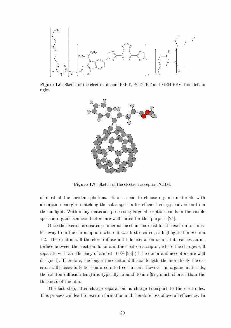
the acceptor material under the PCBM molecular structure (see figure 1.7).

Current generation from solar energy is achieved in four steps [95]. First, the

incident light must be absorbed by the solar cell to create an exciton. As we have

seen above, organic semiconductors possess very good absorption properties, and

therefore thin-film layers of typically 100 nm [96] are thick enough for absorption

19

n

⎡

⎣

⎢⎢⎢⎢⎢⎢⎢⎢⎢⎢

⎤

⎦

⎥⎥⎥⎥⎥⎥⎥⎥⎥⎥

H17C8

C8H17

N N

NS S

Figure 1.6: Sketch of the electron donors P3HT, PCDTBT and MEH-PPV, from left toright.

Figure 1.7: Sketch of the electron acceptor PCBM.

of most of the incident photons. It is crucial to choose organic materials with

absorption energies matching the solar spectra for efficient energy conversion from

the sunlight. With many materials possessing large absorption bands in the visible

spectra, organic semiconductors are well suited for this purpose [24].

Once the exciton is created, numerous mechanisms exist for the exciton to trans-

fer away from the chromophore where it was first created, as highlighted in Section

1.2. The exciton will therefore diffuse until de-excitation or until it reaches an in-

terface between the electron donor and the electron acceptor, where the charges will

separate with an efficiency of almost 100% [93] (if the donor and acceptors are well

designed). Therefore, the longer the exciton diffusion length, the more likely the ex-

citon will successfully be separated into free carriers. However, in organic materials,

the exciton diffusion length is typically around 10 nm [97], much shorter than the

thickness of the film.

The last step, after charge separation, is charge transport to the electrodes.

This process can lead to exciton formation and therefore loss of overall efficiency. In

20

organic materials, due to the low charge mobilities (from 10−5 to 10−2 cm2 ·V−1 · s−1

[86]), the charge collection length is also less than 100 nm, making it difficult for

this process to occur in a typical solar cell.

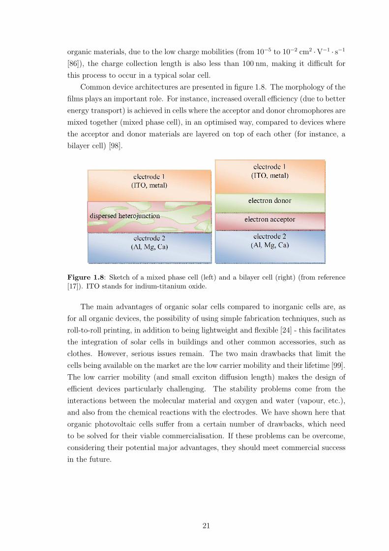
Common device architectures are presented in figure 1.8. The morphology of the

films plays an important role. For instance, increased overall efficiency (due to better

energy transport) is achieved in cells where the acceptor and donor chromophores are

mixed together (mixed phase cell), in an optimised way, compared to devices where

the acceptor and donor materials are layered on top of each other (for instance, a

bilayer cell) [98].

Figure 1.8: Sketch of a mixed phase cell (left) and a bilayer cell (right) (from reference[17]). ITO stands for indium-titanium oxide.

The main advantages of organic solar cells compared to inorganic cells are, as

for all organic devices, the possibility of using simple fabrication techniques, such as

roll-to-roll printing, in addition to being lightweight and flexible [24] - this facilitates

the integration of solar cells in buildings and other common accessories, such as

clothes. However, serious issues remain. The two main drawbacks that limit the

cells being available on the market are the low carrier mobility and their lifetime [99].

The low carrier mobility (and small exciton diffusion length) makes the design of

efficient devices particularly challenging. The stability problems come from the

interactions between the molecular material and oxygen and water (vapour, etc.),

and also from the chemical reactions with the electrodes. We have shown here that

organic photovoltaic cells suffer from a certain number of drawbacks, which need

to be solved for their viable commercialisation. If these problems can be overcome,

considering their potential major advantages, they should meet commercial success

in the future.

21

1.3.3 Organic light emitting diodes (OLEDs)

The most commercially successful device to date is without question the or-

ganic light emitting diode (OLED) [24]. Electrolumiscence was achieved in organic

crystals in 1965 [100], but the first thin-film OLED created by vacuum deposited

molecular materials dates from 1987 [5], and the first OLED from solution processed

polymers was realised in 1990 [101]. After the demonstration of these functioning

devices, research has been focused on using OLEDs for displays, and such displays

can already be found on the market. In addition, since the beginning of the twenty-

first century, numerous researchers have investigated the utilisation of OLEDs for

lighting purposes [102–105].

The fundamental principles of OLEDs are in many respects the same as for a

photovoltaic cell, except that an OLED operates in “reverse-mode”. Indeed the

injection of electric energy into an OLED creates an emission of photons. The steps

leading to light emission are [106]: application of an external voltage for the injection

of free charges through the electrodes of the OLED, transport of these free charges in

the device, leading to exciton formation, and finally radiative decay of this exciton.

The injection of the free carriers is realised by two electrodes situated at opposite

sides of the device. As for solar cells, at least one of these electrodes needs to be

transparent. ITO (indium-titanium oxide) is very commonly used as the anode [107],

as it is a high work-function transparent metal. After injection of the holes at the

anode, the holes will fill the HOMOs of the chromophores of a conduction layer,

the hole-transport layer. This layer needs a high mobility to guarantee efficient

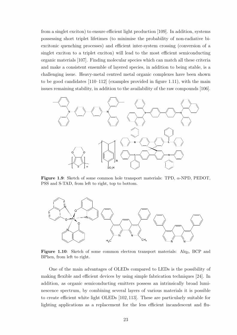
transport of the holes away from the anode. TPD, α-NPD, PEDOT:PSS and S-

TAD are common materials used for hole transports [106] (see figure 1.9). Similarly,

electrons are injected from the cathode (usually made of aluminium, magnesium

or silver [107]), before being transported further away by the electron transport

layer, where the electrons will fill the LUMOs of the semiconductors of this region.

Materials used for electron transport are for instance Alq3, BCP or BPhen [106] (see

figure 1.10). Having these extra electron or hole transport layers could be seen as

problematic for the overall efficiency of the device; however, this in fact enables an

efficiency improvement if all the layer materials and thickness are well chosen and

tuned [106]. After transport of the free charges through the transport layer, the

free charges reach the recombination region where they need to “meet” (enter their

Coulombic attraction region) in order to form excitons. Due to the multiplicity of

three of the triplet states, three quarters of the excitons formed in this way will be

triplets states, with only one quarter being singlet excitons [108]. Therefore, the

molecular species in the recombination region need to be efficient phosphorescent

materials (radiative decay from a triplet state) rather than fluorescent (light emission

22

from a singlet exciton) to ensure efficient light production [109]. In addition, systems

possessing short triplet lifetimes (to minimise the probability of non-radiative bi-

excitonic quenching processes) and efficient inter-system crossing (conversion of a

singlet exciton to a triplet exciton) will lead to the most efficient semiconducting

organic materials [107]. Finding molecular species which can match all these criteria

and make a consistent ensemble of layered species, in addition to being stable, is a

challenging issue. Heavy-metal centred metal organic complexes have been shown

to be good candidates [110–112] (examples provided in figure 1.11), with the main

issues remaining stability, in addition to the availability of the raw compounds [106].

Figure 1.9: Sketch of some common hole transport materials: TPD, α-NPD, PEDOT,PSS and S-TAD, from left to right, top to bottom.

Figure 1.10: Sketch of some common electron transport materials: Alq3, BCP andBPhen, from left to right.

One of the main advantages of OLEDs compared to LEDs is the possibility of

making flexible and efficient devices by using simple fabrication techniques [24]. In

addition, as organic semiconducting emitters possess an intrinsically broad lumi-

nescence spectrum, by combining several layers of various materials it is possible

to create efficient white light OLEDs [102, 113]. These are particularly suitable for

lighting applications as a replacement for the less efficient incandescent and flu-

23

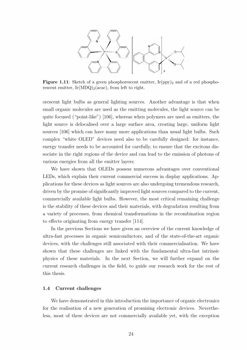
Figure 1.11: Sketch of a green phosphorescent emitter, Ir(ppy)3 and of a red phospho-rescent emitter, Ir(MDQ)2(acac), from left to right.

orescent light bulbs as general lighting sources. Another advantage is that when

small organic molecules are used as the emitting molecules, the light source can be

quite focused (“point-like”) [106], whereas when polymers are used as emitters, the

light source is delocalised over a large surface area, creating large, uniform light

sources [106] which can have many more applications than usual light bulbs. Such

complex “white OLED” devices need also to be carefully designed: for instance,

energy transfer needs to be accounted for carefully, to ensure that the excitons dis-

sociate in the right regions of the device and can lead to the emission of photons of

various energies from all the emitter layers.

We have shown that OLEDs possess numerous advantages over conventional

LEDs, which explain their current commercial success in display applications. Ap-

plications for these devices as light sources are also undergoing tremendous research,

driven by the promise of significantly improved light sources compared to the current,

commercially available light bulbs. However, the most critical remaining challenge

is the stability of these devices and their materials, with degradation resulting from

a variety of processes, from chemical transformations in the recombination region

to effects originating from energy transfer [114].

In the previous Sections we have given an overview of the current knowledge of

ultra-fast processes in organic semiconductors, and of the state-of-the-art organic

devices, with the challenges still associated with their commercialisation. We have

shown that these challenges are linked with the fundamental ultra-fast intrinsic

physics of these materials. In the next Section, we will further expand on the

current research challenges in the field, to guide our research work for the rest of

this thesis.

1.4 Current challenges

We have demonstrated in this introduction the importance of organic electronics

for the realisation of a new generation of promising electronic devices. Neverthe-

less, most of these devices are not commercially available yet, with the exception

24

of OLEDs which are available in only one area of their two possible uses. From

the introduction, it is clear that the current research challenges are numerous and

particularly arduous for the route to mass-produced, commercially available de-

vices. These challenges cover a wide area of science, with physics, chemistry and

engineering being the fundamental disciplines that enable the understanding and

improvement of these materials. For instance, it is crucial to develop new materials

with improved intrinsic properties, such as an increased charge mobility or charge-

transfer character [115], in addition to being easy to synthesise and to process, with

widely available, cheap compounds [115]. These materials and device structures

also need to be stable under repeated electrical- or photo-excitations, and to not

chemically react with other species (such as oxygen or water) in a time-span which

should ensure a good device life-time [115]. Control of the fabrication processes also

needs to be improved [115] to avoid batch to batch variations, and to realise more

efficient device morphologies. Indeed, fundamental questions about morphologies

still remain (what is a typical polymer morphology in films, and how does this affect

its semiconducting properties?). The way electron donor and acceptor polymers

are blended in solar cells is still not clear [116], for instance. Similarly, the role of

interfaces in the efficiency of a device is very complex and far from being elucidated.

More generally, very fundamental physics issues remain. One major issue is

the role of energy transfer in organic systems, and the difficulties in modelling such

processes - as highlighted in Section 1.2.3, these mechanisms are complex and in-

volve many parameters and approximations - for instance identifying the appropriate

transfer regime. Analytical models are still emerging and are far from being able

to simulate the physics of a real system [117], especially as in-depth observation of

energy transfer is not often directly accessible experimentally. However, the avail-

ability of such analytical models, and, for instance, the understanding of the role

of coherent versus incoherent regimes in energy transfer, would definitely help to

improve devices. In addition, coherent effects are still not well understood, and

extensive research remains to be undertaken to understand the early stage of exci-

ton creation, such as to what extent the coherent exciton is delocalised and where

and how the exciton localises when decoherence appears [31]. More generally, many

ultra-fast physical processes (exciton creation, charge separation, molecular relax-

ation and energy transfer, among others) take place in typically sub-picosecond

time-scales [118–122], making experimental probes of such processes particularly

challenging, and consequently, theoretical formulations are not easily verifiable by

experiments.

Excited-state processes are also very difficult to model and therefore theoretical

knowledge of such processes is very limited [123]. However, they play an important

role in the physics of the device, through phenomena like, among others, excited-

25

state absorption, damages by ionisation or exciton-exciton annihilation.

1.5 Aim of the thesis

We have shown the importance of organic semiconducting materials for the reali-

sation of a new generation of devices which are extremely promising as a replacement

for conventional, inorganic semiconductor devices. We have seen that the challenges

facing the fabrication of commercially-ready organic devices are still numerous, and

require the collaboration of many disciplines, such as process engineering for improv-

ing the actual fabrication steps of the devices, to fundamental physics to understand

the mechanisms responsible for the intrinsic properties of the materials.

In this thesis, to address some of these challenges, we will focus on the fundamen-

tal physical aspects, and study the theory of exciton transfer in a single, star-shaped

molecule (Chapters 3 and 4) and in an ensemble of chromophores mimicking a poly-

mer thin-film (Chapters 5 and 6). These star-shaped molecules are a novel class

of fluorene-based materials that increase the ease of experimental processing. The

polymer is polyfluorene, currently very often used because of its good physical prop-

erties, and because it constitutes a good model system (see Chapter 2). We will

confront these theoretical studies with experimental results from our collaborators

at the university of St Andrews. We aim to model exciton transfer in a realistic

way to obtain useful knowledge about the important mechanisms that govern such

transfers.

In the next Chapter, we present the theoretical methods that we will use to

achieve these goals.

26

Chapter 2

Methods

In this Chapter, we introduce the methods that are used in the rest of the

research presented in this thesis. Indeed, in order to successfully model and un-

derstand the theory of ultra-fast photo-physics in organic semiconductors, reliable

methods and a study of preliminary basic concepts are necessary to underpin any

deep theory work.

2.1 Introduction

In the field of organic semiconductor theory, there are some well-established

theoretical methods which describe the quantum effects regulating the properties of

small molecular systems, or the structure-related properties of larger systems. They

are usually referred to as “Quantum Chemistry” (QC) [124], and will be presented in

Sections 2.2 and 2.3. In this thesis, if not indicated otherwise, “system” designates

an isolated ensemble of atoms, for instance one molecule (typically, a “small system”)

or an ensemble of thousands of interacting molecules (a “large system”).

However, the description of the photophysics of a large system is a much more

complex problem, and an important current research topic [125]. Two main ap-

proaches prevail in modelling the photo-physics of organic semiconductors: a method

based on the Monte-Carlo simulation of charges or quasi-particles (such as excitons)

moving around in the system [126–134]; and a method based on a master-equation

type approach, which enables the calculation of the evolution of exciton densities

at the microscopic level [125,135–138]. The approach used in this work being much

closer to this latter method, the Monte-Carlo method will not be developed in this

Section. A simple master-equation type approach, the “Optical Bloch Equations”

(OBE), is presented in Section 2.4 to introduce some generic approximations and

results that will be used in the rest of this thesis.

We are interested in the photo-physics of molecular systems. Therefore we aim

to calculate molecular transition properties, such as energy, dipole and density, and

time-dependent excitonic properties, such as polarisation or the exciton densities

of large ensembles of molecules. The former quantities will be obtained by the

electronic structure methods presented in Section 2.3 and the later time-dependent

properties will be calculated by the OBE, as presented in Section 2.4.

27

2.2 Quantum chemistry

2.2.1 Large-scale atomistic systems methods

These methods, for the investigation of a large atomistic system (thousands of

atoms), usually enable either access to information on the structural properties or

predict the time-dependent photo-physics of an ensemble of chromophores. The

methods used to obtain the structural details are generally referenced under the

name “Molecular Dynamics” (MD) or sometimes “Molecular Mechanics” (MM).

They are mostly based on classical physics: they use a force-field to obtain the

electronic energy as a function of the position of the nuclear coordinates, and use

Newton’s Law to describe the nuclear motions [124, 139]. These methods therefore

enable time-dependent simulations of the interactions between a large number of

atomistic and molecular components at low computational cost. They enable, for

instance, the calculation of geometries, relative energies (such as torsional or bending

energies) and energy barriers for interconversion between different conformations.

They have been applied successfully in biology and biophysics to study large-scale

processes, such as protein folding or interactions [140, 141], but their application

to organic semiconductors is more recent [142] and their reliability is therefore not

as well-established. Indeed, the correct force field for such components is usually

not known. For this reason, these methods have not been used at any stage of the

research work presented here and so will not be described in more detail in this

thesis.

2.2.2 Small-scale atomistic systems methods

The methods dealing with a small-scale atomistic system are usually described

under the generic term “electronic structure methods” [124, 143]. This term covers

common methods such as the Hartree-Fock approximation or Density-Functional

Theory (DFT), and are typically used for calculating the electronic and vibrational

properties of a single molecule. We have been using these methods extensively in

our research to predict the electronic properties of a number of polyfluorene-based

molecules. For this reason, in Section 2.3, we will review, in detail, the basics of

electronic structure methods calculations, and how they have been used to produce

some of the results presented later in this thesis.

28

2.3 QC: Electronic structure methods

2.3.1 Background

Electronic structure methods encompass a very wide range of methods, approx-

imations and techniques, with the aim of predicting, as accurately and efficiently

as possible, the quantum-related properties of any molecule (including geometric or

electronic properties [124]). The goal is simply to calculate the solution of the M -

particle Schrodinger equation Hφi(r1, r2, . . . , rM ) = εiφi(r1, r2, . . . , rM , t), where

H is the Hamiltonian of the system, φi the M -body wavefunction of the i-th excited-

state and εi its energy, from which it is possible to derive all other system properties.

The Hamiltonian is the sum of the kinetic and potential energy terms: H = T + V ,

the potential energy V being the Coulomb interaction between each pair of charged

entities, and the kinetic energy T being the sum of the individual kinetic energies

of each particle in the molecule.

Unfortunately, for molecules it is impossible to solve this Schrodinger equation

exactly. The electronic structure methods aim at making this solution tractable with

modern computers, at the price of some approximations. These electronic structure

methods are divided into three categories [143]: semi-empirical methods, ab-initio

methods and Density Functional Theory (DFT).

Two approximations are common to any electronic structure method [144]: the

adiabatic approximation and the Born-Oppenheimer approximation. In the adia-

batic approximation [145], the coupling between different electronic states is ne-

glected; systems involving these electronic states coupling are photochemical reac-

tions and beyond the scope of this work. The Born-Oppenheimer approximation

goes further than the adiabatic approximation, by stating that, as the nuclei are

much heavier than the electrons (by at least a factor of a few thousand), the move-

ments of the nuclei can be neglected compared to the movement of the electrons [146].

The kinetic energy of the nuclei is thus assumed to be zero and the electronic motion

is described as occurring in a field of fixed nuclei. This means that the total Hamil-

tonian for the M -particle system can be rewritten as H = Helec, Helec depending

only on the N electrons in the system. It is also important to note that the particles

are considered as non-relativistic.

The further principles and differences between the three methods are presented

in the following Subsections, with a particular emphasis on DFT, as this is the

method we have been using to obtain our theoretical knowledge of the fluorene-

based molecules presented in the rest of this thesis.

29

Semi-empirical methods

Semi-empirical methods are based on a series of experimental parameters, to

simplify the solution of the Schrodinger equation [144], but nonetheless keeping

it realistic. Examples of common methods include the Austin Model 1 (AM1) or

Modified Neglect of Diatomic Overlap (MNDO). However, these methods are by

essence very sensitive to the system they are employed for [144]. Indeed, they are

parametrised from experimental data for a system of molecules, and the results they

produce can only be trusted if the system studied theoretically is very “close” to

the experimental system which parametrised the method - “close” being difficult to

quantify. Despite being computationally inexpensive, we decided not to use these

methods because of this aforementioned limitation: for instance, the star-shaped

truxene-cored molecules we investigated, presented in the next Chapter, have not

been extensively studied and they have been relatively recently synthesized [37];

therefore parametrising a semi-empirical method would have been challenging and

without any guarantee of success.

Ab-initio methods

Ab-initio methods, on the other hand, do not involve any experimental results

in their algorithms, but are based solely on the laws of quantum mechanics and

theoretical properties obtained using these laws [144]. The most popular methods

in this category are the Configuration Interaction method (CI), the Møller-Plesser

perturbation theory (MP) and the Coupled Cluster Methods such as CCSD and

CCSD(T). These methods are better than the semi-empirical methods in the sense

that, as they do not rely on experimental data, they can be used on any kind

of system [124]. However, the computational cost of such methods is much higher

than for semi-empirical methods [144], making then less practical for large molecules

(more than 10 atoms for CCSD(T), more than a hundred for CI). For this reason, we

have not been using any of these ab-initio methods, but instead used the more recent

DFT, which offers a good compromise between computational cost and accuracy,

and is for this reason already very popular.

Density Functional Theory

Rather than directly calculating the wavefunction from the Schrodinger equa-

tion, like the semi-empirical methods and ab-initio methods do, DFT calculates the

charge density of the system, from which it is possible to obtain the wavefunctions.

Indeed, DFT is based on the theorem demonstrated by Hohenberg and Kohn [147].

This theorem states that the potential of an interacting system is fully determined

by its electronic density, and that there is a functional expressing the total energy

30

as a function of the electronic density, valid for any potential. For a particular po-

tential, the energy minimising the functional is the energy of the ground state, and

its associated density is the ground state density.

The main advantage of this theorem is that the many-body problem (N electrons

and therefore 3N variables) can be simplified into a single-body problem with only

three variables, as only the one-particle probability density is necessary to obtain

all the information about the ground-state. This single-particle probability density

n(r) is defined as:

n(r) = N

∫...

∫|φi(r, r2, . . . , rN )|2 d3r2. . . d3rN . (2.1)

The difficulty is now to obtain the one-particle density of the system. This can

be done relatively easily by the Kohn-Sham algorithm [148]. The work realised by

Kohn and Sham consists of separating the total electronic energy Helec[n] into the

kinetic energy Telec and the electronic potential energy V [n], itself divided into the

series of following terms ([n] designates a functional of n):

Helec[n] = Telec + V [n] = Telec + Vnn + Ven + Vee + VXC [n] , (2.2)

where Telec is the kinetic energy of the electrons, given by:

Telec = −∑

i

~2

2m∇2

i , (2.3)

Vnn is the Coulomb interaction between the nuclei. In the frame of the Born-

Oppenheimer interaction, this term is constant.

Ven is the nuclear-electron Coulomb interaction, and of course depends on the elec-

tron density n(r):

Ven =e2

4πε0

∑

i

∫Zin(r)

|Ri − r|dr , (2.4)

where Zi is the charge of nuclei i and Ri its centre. Vee is the electron-electron

Coulomb interaction, depending on n(r):

Vee =e2

4πε0

∑

i

1

2

∫ ∫n(r)n(r′)

|r − r′| drdr′ . (2.5)

VXC [n] is the exchange-correlation term, which can be further decomposed into

the exchange term VX [n] and the correlation term VC [n] [143]: VXC [n] = VX [n] +

VC [n]. VX [n] is the exchange energy arising from the antisymmetry of the electronic

wavefunctions and VC [n] is the dynamic correlation in the motions of the individual

31

electrons. This term VXC is the functional that gave its name to DFT. It is a

functional in the sense that it is a function of a function. Indeed, this potential

VXC [n] is not known exactly and therefore many alternatives exist to calculate it.

They will be detailed in Section 2.3.2.

In practice, the steps of the Kohn-Sham algorithm, which enables the calcu-

lation of the electronic density and therefore the electronic wavefunctions, are the

following [143]:

1) Guess of an initial electron density n(r).

2) Calculation of the effective potential V [n] = Vnn + Ven + Vee + VXC [n].

3) Solving the Schrodinger equation:

Helec[n] (r1, · , rN , )φi (r1, . . . , rN , ) = ǫiφi (r1, . . . , rN , ) , (2.6)

which provides the electronic wavefunctions φi (r1, · , rN , ) and energies ǫi.

4) Calculation of the new electronic density using:

n∗ (r) =N∑

i

|φi (r)|2 . (2.7)

5) If the new electronic density n∗ (r) is very close to n (r), then the problem is

solved; otherwise we iterate starting from step 2) until convergence is achieved.

This method would therefore be exact (with the exception of approximations

such as the Born-Oppenheimer approximation mentioned previously) if we knew how

to express the exchange-correlation potential. This is not the case, and this is the

main limitation of DFT: knowing how to express this exchange-correlation potential

and thus which functional to use. The inclusion of such a corrective term is still a

strong point of DFT, compared for instance to methods such as Hartee-Fock, where

the correlation is calculated on average, using a mean-field electron density, and the

way it is included in the theory means it is much more computationally efficient

than ab-initio methods. This explains the popularity of DFT: almost obtaining

the accuracy of ab-initio methods, at only the computational cost of semi-empirical

methods.

It is worth noting that this method deals with the ground-state only. How-

ever, most phenomena relevant for the photo-physics study of molecules are excited-

state processes. Fortunately, a method based on DFT was recently developed to

32

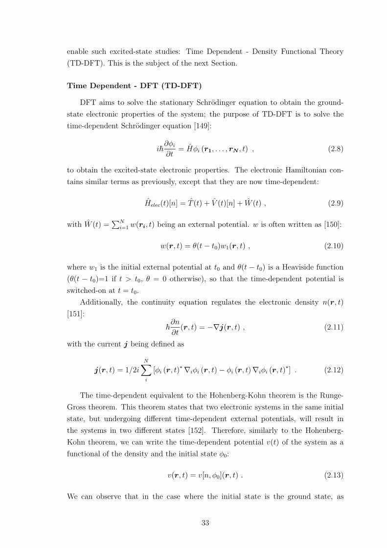
enable such excited-state studies: Time Dependent - Density Functional Theory

(TD-DFT). This is the subject of the next Section.

Time Dependent - DFT (TD-DFT)

DFT aims to solve the stationary Schrodinger equation to obtain the ground-

state electronic properties of the system; the purpose of TD-DFT is to solve the

time-dependent Schrodinger equation [149]:

i~∂φi

∂t= Hφi (r1, . . . , rN , t) , (2.8)

to obtain the excited-state electronic properties. The electronic Hamiltonian con-

tains similar terms as previously, except that they are now time-dependent:

Helec(t)[n] = T (t) + V (t)[n] + W (t) , (2.9)

with W (t) =∑N

i=1 w(ri, t) being an external potential. w is often written as [150]:

w(r, t) = θ(t− t0)w1(r, t) , (2.10)

where w1 is the initial external potential at t0 and θ(t− t0) is a Heaviside function

(θ(t − t0)=1 if t > t0, θ = 0 otherwise), so that the time-dependent potential is

switched-on at t = t0.

Additionally, the continuity equation regulates the electronic density n(r, t)

[151]:

~∂n

∂t(r, t) = −∇j(r, t) , (2.11)

with the current j being defined as

j(r, t) = 1/2iN∑

i

[φi (r, t)∗∇iφi (r, t)− φi (r, t)∇iφi (r, t)

∗] . (2.12)

The time-dependent equivalent to the Hohenberg-Kohn theorem is the Runge-

Gross theorem. This theorem states that two electronic systems in the same initial

state, but undergoing different time-dependent external potentials, will result in

the systems in two different states [152]. Therefore, similarly to the Hohenberg-

Kohn theorem, we can write the time-dependent potential v(t) of the system as a

functional of the density and the initial state φ0:

v(r, t) = v[n, φ0](r, t) . (2.13)

We can observe that in the case where the initial state is the ground state, as

33

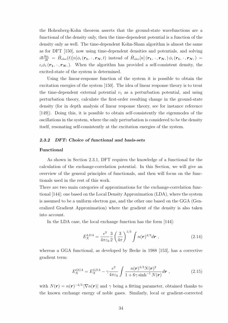
the Hohenberg-Kohn theorem asserts that the ground-state wavefunctions are a

functional of the density only, then the time-dependent potential is a function of the

density only as well. The time-dependent Kohn-Sham algorithm is almost the same

as for DFT [150], now using time-dependent densities and potentials, and solving

i~∂φi

∂t= Helec(t)[n]φi (r1, · , rN , t) instead of Helec[n] (r1, · , rN , )φi (r1, · , rN , ) =

ǫiφi (r1, · , rN , ). When the algorithm has provided a self-consistent density, the

excited-state of the system is determined.

Using the linear-response function of the system it is possible to obtain the

excitation energies of the system [150]. The idea of linear response theory is to treat

the time-dependent external potential v1 as a perturbation potential, and using

perturbation theory, calculate the first-order resulting change in the ground-state

density (for in depth analysis of linear response theory, see for instance reference

[149]). Doing this, it is possible to obtain self-consistently the eigenmodes of the

oscillations in the system, where the only perturbation is considered to be the density

itself, resonating self-consistently at the excitation energies of the system.

2.3.2 DFT: Choice of functional and basis-sets

Functional

As shown in Section 2.3.1, DFT requires the knowledge of a functional for the

calculation of the exchange-correlation potential. In this Section, we will give an

overview of the general principles of functionals, and then will focus on the func-

tionals used in the rest of this work.

There are two main categories of approximations for the exchange-correlation func-

tional [144]; one based on the Local Density Approximation (LDA), where the system

is assumed to be a uniform electron gas, and the other one based on the GGA (Gen-

eralized Gradient Approximation) where the gradient of the density is also taken

into account.

In the LDA case, the local exchange function has the form [144]:

ELDAX =

e2

4πε0

3

2

(3

4π

)1/3 ∫n(r)4/3dr , (2.14)

whereas a GGA functional, as developed by Becke in 1988 [153], has a corrective

gradient term:

EGGAX = ELDA

X − γe2

4πε0

∫n(r)4/3N(r)2

1 + 6γ sinh−1 N(r)dr , (2.15)

with N(r) = n(r)−4/3 |∇n(r)| and γ being a fitting parameter, obtained thanks to

the known exchange energy of noble gases. Similarly, local or gradient-corrected

34

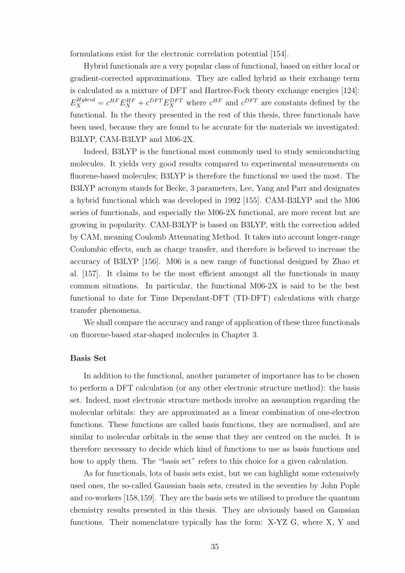
formulations exist for the electronic correlation potential [154].

Hybrid functionals are a very popular class of functional, based on either local or

gradient-corrected approximations. They are called hybrid as their exchange term

is calculated as a mixture of DFT and Hartree-Fock theory exchange energies [124]:

EHybridX = cHFEHF

X + cDFTEDFTX where cHF and cDFT are constants defined by the

functional. In the theory presented in the rest of this thesis, three functionals have

been used, because they are found to be accurate for the materials we investigated:

B3LYP, CAM-B3LYP and M06-2X.

Indeed, B3LYP is the functional most commonly used to study semiconducting

molecules. It yields very good results compared to experimental measurements on

fluorene-based molecules; B3LYP is therefore the functional we used the most. The

B3LYP acronym stands for Becke, 3 parameters, Lee, Yang and Parr and designates

a hybrid functional which was developed in 1992 [155]. CAM-B3LYP and the M06

series of functionals, and especially the M06-2X functional, are more recent but are

growing in popularity. CAM-B3LYP is based on B3LYP, with the correction added

by CAM, meaning Coulomb Attenuating Method. It takes into account longer-range

Coulombic effects, such as charge transfer, and therefore is believed to increase the

accuracy of B3LYP [156]. M06 is a new range of functional designed by Zhao et

al. [157]. It claims to be the most efficient amongst all the functionals in many

common situations. In particular, the functional M06-2X is said to be the best

functional to date for Time Dependant-DFT (TD-DFT) calculations with charge

transfer phenomena.

We shall compare the accuracy and range of application of these three functionals

on fluorene-based star-shaped molecules in Chapter 3.

Basis Set

In addition to the functional, another parameter of importance has to be chosen

to perform a DFT calculation (or any other electronic structure method): the basis

set. Indeed, most electronic structure methods involve an assumption regarding the

molecular orbitals: they are approximated as a linear combination of one-electron

functions. These functions are called basis functions, they are normalised, and are

similar to molecular orbitals in the sense that they are centred on the nuclei. It is

therefore necessary to decide which kind of functions to use as basis functions and

how to apply them. The “basis set” refers to this choice for a given calculation.

As for functionals, lots of basis sets exist, but we can highlight some extensively

used ones, the so-called Gaussian basis sets, created in the seventies by John Pople

and co-workers [158,159]. They are the basis sets we utilised to produce the quantum

chemistry results presented in this thesis. They are obviously based on Gaussian

functions. Their nomenclature typically has the form: X-YZ G, where X, Y and

35

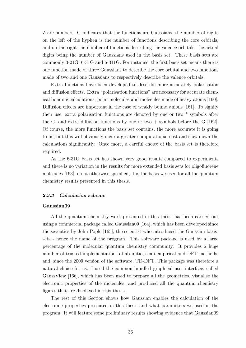
Z are numbers. G indicates that the functions are Gaussians, the number of digits

on the left of the hyphen is the number of functions describing the core orbitals,

and on the right the number of functions describing the valence orbitals, the actual

digits being the number of Gaussians used in the basis set. These basis sets are

commonly 3-21G, 6-31G and 6-311G. For instance, the first basis set means there is

one function made of three Gaussians to describe the core orbital and two functions

made of two and one Gaussians to respectively describe the valence orbitals.

Extra functions have been developed to describe more accurately polarisation

and diffusion effects. Extra “polarisation functions” are necessary for accurate chem-

ical bonding calculations, polar molecules and molecules made of heavy atoms [160].

Diffusion effects are important in the case of weakly bound anions [161]. To signify

their use, extra polarisation functions are denoted by one or two * symbols after

the G, and extra diffusion functions by one or two + symbols before the G [162].

Of course, the more functions the basis set contains, the more accurate it is going

to be, but this will obviously incur a greater computational cost and slow down the

calculations significantly. Once more, a careful choice of the basis set is therefore

required.

As the 6-31G basis set has shown very good results compared to experiments

and there is no variation in the results for more extended basis sets for oligofluorene

molecules [163], if not otherwise specified, it is the basis we used for all the quantum

chemistry results presented in this thesis.

2.3.3 Calculation scheme

Gaussian09

All the quantum chemistry work presented in this thesis has been carried out

using a commercial package called Gaussian09 [164], which has been developed since

the seventies by John Pople [165], the scientist who introduced the Gaussian basis-

sets - hence the name of the program. This software package is used by a large

percentage of the molecular quantum chemistry community. It provides a huge

number of trusted implementations of ab-initio, semi-empirical and DFT methods,

and, since the 2009 version of the software, TD-DFT. This package was therefore a

natural choice for us. I used the common bundled graphical user interface, called

GaussView [166], which has been used to prepare all the geometries, visualise the

electronic properties of the molecules, and produced all the quantum chemistry

figures that are displayed in this thesis.

The rest of this Section shows how Gaussian enables the calculation of the

electronic properties presented in this thesis and what parameters we used in the

program. It will feature some preliminary results showing evidence that Gaussian09

36

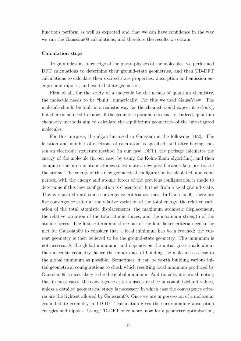
functions perform as well as expected and that we can have confidence in the way

we run the Gaussian09 calculations, and therefore the results we obtain.

Calculation steps

To gain relevant knowledge of the photo-physics of the molecules, we performed

DFT calculations to determine their ground-state geometries, and then TD-DFT

calculations to calculate their excited-state properties: absorption and emission en-

ergies and dipoles, and excited-state geometries.

First of all, for the study of a molecule by the means of quantum chemistry,

the molecule needs to be “built” numerically. For this we used GaussView. The

molecule should be built in a realistic way (as the chemist would expect it to look),

but there is no need to know all the geometric parameters exactly. Indeed, quantum

chemistry methods aim to calculate the equilibrium geometries of the investigated

molecules.

For this purpose, the algorithm used in Gaussian is the following [162]. The

location and number of electrons of each atom is specified, and after having cho-

sen an electronic structure method (in our case, DFT), the package calculates the

energy of the molecule (in our case, by using the Kohn-Sham algorithm), and then

computes the internal atomic forces to estimate a new possible and likely position of

the atoms. The energy of this new geometrical configuration is calculated, and com-

parison with the energy and atomic forces of the previous configuration is made to

determine if this new configuration is closer to or further from a local ground-state.

This is repeated until some convergence criteria are met. In Gaussian09, there are

five convergence criteria: the relative variation of the total energy, the relative vari-

ation of the total atomistic displacements, the maximum atomistic displacement,

the relative variation of the total atomic forces, and the maximum strength of the

atomic forces. The first criteria and three out of the four latter criteria need to be

met for Gaussian09 to consider that a local minimum has been reached; the cur-

rent geometry is then believed to be the ground-state geometry. This minimum is

not necessarily the global minimum, and depends on the initial guess made about

the molecular geometry, hence the importance of building the molecule as close to

the global minimum as possible. Sometimes, it can be worth building various ini-

tial geometrical configurations to check which resulting local minimum produced by

Gaussian09 is most likely to be the global minimum. Additionally, it is worth noting

that in most cases, the convergence criteria used are the Gaussian09 default values,

unless a detailed geometrical study is necessary, in which case the convergence crite-

ria are the tightest allowed by Gaussian09. Once we are in possession of a molecular

ground-state geometry, a TD-DFT calculation gives the corresponding absorption

energies and dipoles. Using TD-DFT once more, now for a geometry optimisation,

37

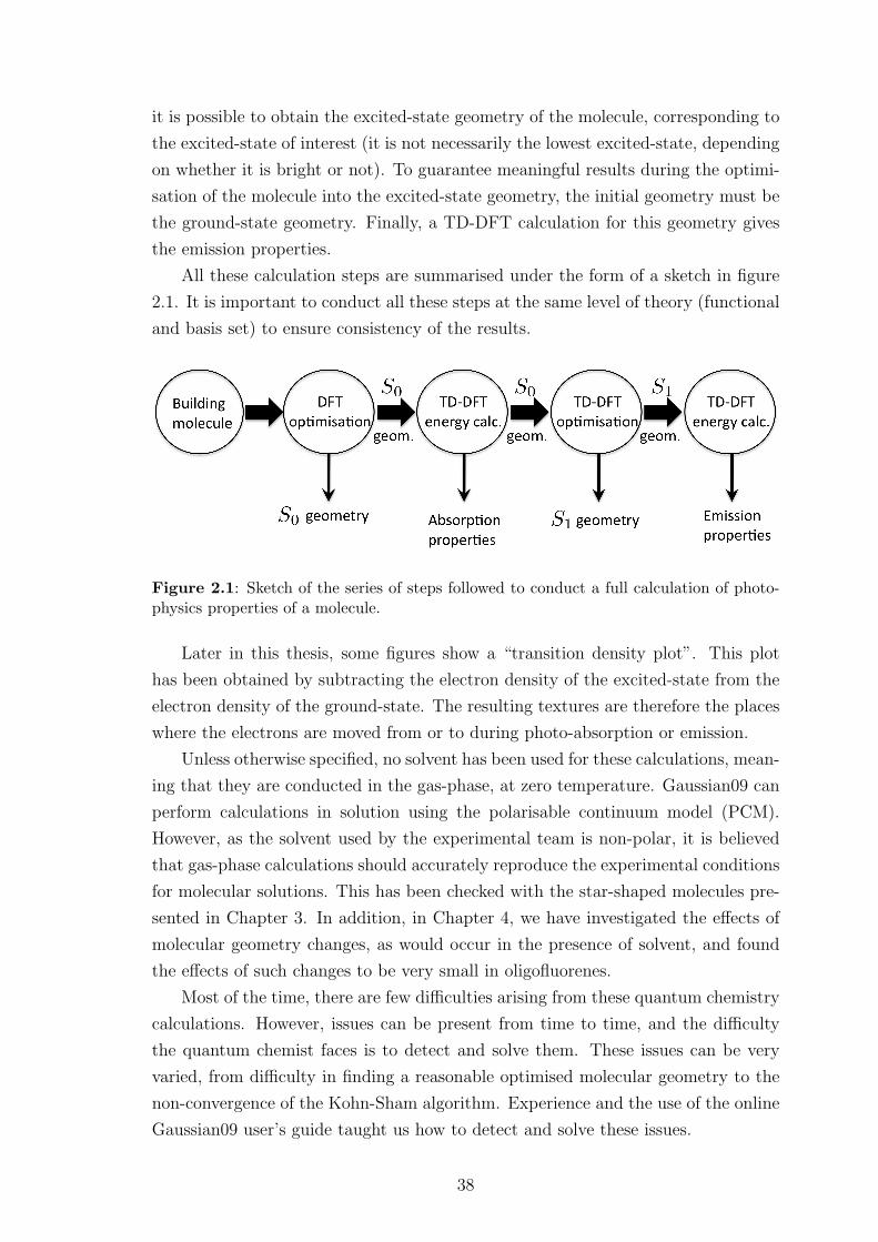
it is possible to obtain the excited-state geometry of the molecule, corresponding to

the excited-state of interest (it is not necessarily the lowest excited-state, depending

on whether it is bright or not). To guarantee meaningful results during the optimi-

sation of the molecule into the excited-state geometry, the initial geometry must be

the ground-state geometry. Finally, a TD-DFT calculation for this geometry gives

the emission properties.

All these calculation steps are summarised under the form of a sketch in figure

2.1. It is important to conduct all these steps at the same level of theory (functional

and basis set) to ensure consistency of the results.

Figure 2.1: Sketch of the series of steps followed to conduct a full calculation of photo-physics properties of a molecule.

Later in this thesis, some figures show a “transition density plot”. This plot

has been obtained by subtracting the electron density of the excited-state from the

electron density of the ground-state. The resulting textures are therefore the places

where the electrons are moved from or to during photo-absorption or emission.

Unless otherwise specified, no solvent has been used for these calculations, mean-

ing that they are conducted in the gas-phase, at zero temperature. Gaussian09 can

perform calculations in solution using the polarisable continuum model (PCM).

However, as the solvent used by the experimental team is non-polar, it is believed

that gas-phase calculations should accurately reproduce the experimental conditions

for molecular solutions. This has been checked with the star-shaped molecules pre-

sented in Chapter 3. In addition, in Chapter 4, we have investigated the effects of

molecular geometry changes, as would occur in the presence of solvent, and found

the effects of such changes to be very small in oligofluorenes.

Most of the time, there are few difficulties arising from these quantum chemistry

calculations. However, issues can be present from time to time, and the difficulty

the quantum chemist faces is to detect and solve them. These issues can be very

varied, from difficulty in finding a reasonable optimised molecular geometry to the

non-convergence of the Kohn-Sham algorithm. Experience and the use of the online

Gaussian09 user’s guide taught us how to detect and solve these issues.

38

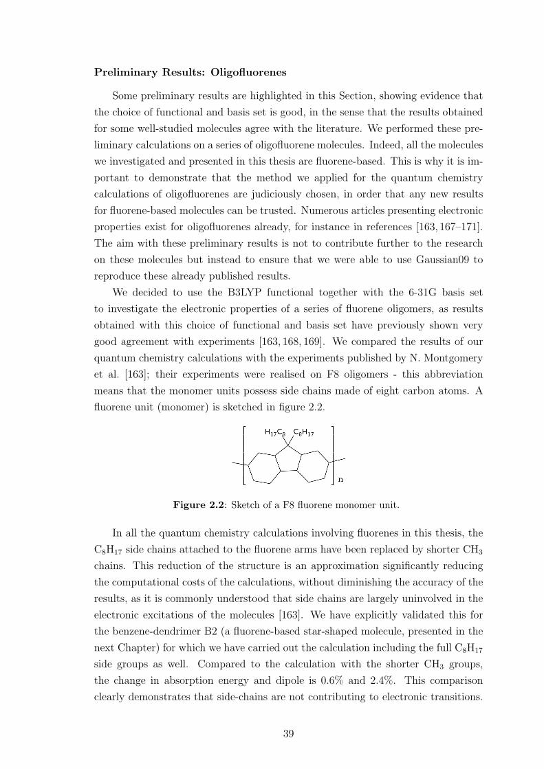
Preliminary Results: Oligofluorenes

Some preliminary results are highlighted in this Section, showing evidence that

the choice of functional and basis set is good, in the sense that the results obtained

for some well-studied molecules agree with the literature. We performed these pre-

liminary calculations on a series of oligofluorene molecules. Indeed, all the molecules

we investigated and presented in this thesis are fluorene-based. This is why it is im-

portant to demonstrate that the method we applied for the quantum chemistry

calculations of oligofluorenes are judiciously chosen, in order that any new results

for fluorene-based molecules can be trusted. Numerous articles presenting electronic

properties exist for oligofluorenes already, for instance in references [163, 167–171].

The aim with these preliminary results is not to contribute further to the research

on these molecules but instead to ensure that we were able to use Gaussian09 to

reproduce these already published results.

We decided to use the B3LYP functional together with the 6-31G basis set

to investigate the electronic properties of a series of fluorene oligomers, as results

obtained with this choice of functional and basis set have previously shown very

good agreement with experiments [163, 168, 169]. We compared the results of our

quantum chemistry calculations with the experiments published by N. Montgomery

et al. [163]; their experiments were realised on F8 oligomers - this abbreviation

means that the monomer units possess side chains made of eight carbon atoms. A

fluorene unit (monomer) is sketched in figure 2.2.

Figure 2.2: Sketch of a F8 fluorene monomer unit.

In all the quantum chemistry calculations involving fluorenes in this thesis, the

C8H17 side chains attached to the fluorene arms have been replaced by shorter CH3

chains. This reduction of the structure is an approximation significantly reducing

the computational costs of the calculations, without diminishing the accuracy of the

results, as it is commonly understood that side chains are largely uninvolved in the

electronic excitations of the molecules [163]. We have explicitly validated this for

the benzene-dendrimer B2 (a fluorene-based star-shaped molecule, presented in the

next Chapter) for which we have carried out the calculation including the full C8H17

side groups as well. Compared to the calculation with the shorter CH3 groups,

the change in absorption energy and dipole is 0.6% and 2.4%. This comparison

clearly demonstrates that side-chains are not contributing to electronic transitions.

39

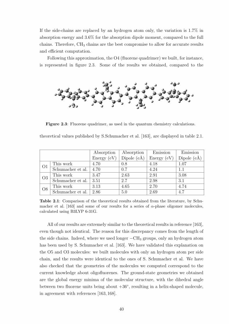
If the side-chains are replaced by an hydrogen atom only, the variation is 1.7% in

absorption energy and 3.6% for the absorption dipole moment, compared to the full

chains. Therefore, CH3 chains are the best compromise to allow for accurate results

and efficient computation.

Following this approximation, the O4 (fluorene quadrimer) we built, for instance,

is represented in figure 2.3. Some of the results we obtained, compared to the

Figure 2.3: Fluorene quadrimer, as used in the quantum chemistry calculations.

theoretical values published by S.Schumacher et al. [163], are displayed in table 2.1.

AbsorptionEnergy (eV)

AbsorptionDipole (eA)

EmissionEnergy (eV)

EmissionDipole (eA)

O1This work 4.70 0.8 4.18 1.07Schumacher et al. 4.70 0.7 4.24 1.1

O3This work 3.47 2.63 2.91 3.08Schumacher et al. 3.51 2.7 2.98 3.1

O8This work 3.13 4.65 2.70 4.74Schumacher et al. 2.86 5.0 2.69 4.7

Table 2.1: Comparison of the theoretical results obtained from the literature, by Schu-macher et al. [163] and some of our results for a series of α-phase oligomer molecules,calculated using B3LYP 6-31G.

All of our results are extremely similar to the theoretical results in reference [163],

even though not identical. The reason for this discrepancy comes from the length of

the side chains. Indeed, where we used longer −CH3 groups, only an hydrogen atom

has been used by S. Schumacher et al. [163]. We have validated this explanation on

the O5 and O3 molecules: we built molecules with only an hydrogen atom per side

chain, and the results were identical to the ones of S. Schumacher et al. We have

also checked that the geometries of the molecules we computed correspond to the

current knowledge about oligofluorenes. The ground-state geometries we obtained

are the global energy minima of the molecular structure, with the dihedral angle

between two fluorene units being about +36, resulting in a helix-shaped molecule,

in agreement with references [163,168].

40

Additionally, comparative checks with an extended basis set (6-31G*) were

made, and the final values always varied by less than 2%. Similar conclusions were

also reached in references [163,169].

These preliminary results enabled us to gain confidence and expertise in the use

of quantum chemistry methods for oligofluorenes. The excellent agreement between

theoretical and experimental transition dipoles and energies, as shown in reference

[163], is obviously preserved by our results. This demonstrates that DFT and TD-

DFT calculations performed at the B3LYP 6-31G level of theory can accurately

describe the physics of oligofluorenes, and therefore fluorene-based molecules.

In summary, we have highlighted the principles of DFT, shown some examples

of the application of this theory with the B3LYP functional, and shown that some

common basis sets obtain good results compared with experiments. This enables

the calculation of the transition dipoles and vertical energies, and the visualisation

of the molecular orbitals, the transition densities and the geometries.

DFT is useful to obtain the properties of single molecules. These properties can

then be utilised for realistic dynamics studies of a few molecules, using the Optical

Bloch Equations (OBE).

2.4 Bloch equations

2.4.1 Background

The optical Bloch equations (OBE) are a version of the original Bloch equations,

which were first developed by Bloch to describe the magnetic resonant effect of

nuclear spin rotation [172]. These were then successfully applied to other physical

systems, for instance predicting the dynamics of a two-level system interacting with

an optical field [173], for inorganic semiconductors [174] and for molecules [175].

The OBE can be written in many ways. We will start by expressing the OBE

as an explicit system of coupled differential equations, to better explore what these

equations govern and imply. Following this we will use the more compact and

practical, but less physically direct, density matrix approach to express the same

equations. The OBE govern the excitation population nXi of the fermionic level i of a

multi-level system X. Typically, the systems we are interested in are chromophores.

The fermionic levels i and j of the same chromophore X are coupled through the

polarization term pXij . Two chromophores X and Y can also be coupled through the

OBE.

In the next Section, we will present how the OBE can be used in practice to

model the photo-physics of organic semiconductors. We will start by presenting the

equation for a simple single two-level system, before introducing a more realistic

six-level system to model an oligofluorene molecule in the next Subsection. Finally,

41

we will present results for systems of these coupled chromophores.

2.4.2 Application for the photo-physics of organic semiconductors

The OBE have been successfully applied to organic systems, for instance for the

modelling of non-interacting oligofluorenes [125] or for the modelling of interacting

light harvesting complexes, such as LHC II [176]. The main advantages of the OBE

is that they include coherences (defined as the off-diagonal term of the density ma-

trix, such as polarisation), and can therefore model coherent effects. They enable

one to gain exact knowledge of the exciton population in a system including vir-

tually any kind of interaction effects (such as exciton diffusion and exciton-exciton

annihilation), and vibrational levels and their relaxation - providing we know all the

necessary parameters (coupling energies, relaxation times, etc.).

The work by Richter et al. [176] consists of modelling the LHC II chromophores

by two-level systems, and then simulating the interactions between fourteen of these

two-level systems. It can predict the ultra-fast photo-physics of such a system, even

at high intensities where Pauli blocking and exciton-exciton annihilation play a

major role in the photo-dynamics. However, real systems of organic semiconductors

cannot be described by such a small number of chromophores. Indeed, organic films

are large-scale systems of interacting chromophores and require, at the very least,

thousands of model chromophores in order to be modelled accurately.

In addition, Schumacher et al. [125] have shown that a two-level model does

not accurately describe an oligofluorene chromophore, as a two-level model does not

account for vibrations. Instead, they used six-level systems, but did not couple them

together, as this would be too computationally expensive.

In the next Section, we will show how to apply the OBE to model organic

electronic systems, introduce results showing the fundamental processes that are

important in such systems, and demonstrate how to implement them accurately in

the OBE. We will also show that an exact formulation of the OBE cannot be utilised

to model large-scale system. However, the OBE still enable one to understand the

theoretical concepts that are needed to establish a simplified yet accurate model.

This simplified model, derived from the OBE, will be the subject of Chapter 6.

2.4.3 Preliminary results

A single two-level system

The Hamiltonian H of a two-level system with energies ε0 and ε1, ε1 > ε0, with

optical pumping, is, using the usual second quantisation operators:

H = ε0c†0c0 + ε1c

†1c1 +

(c†1c0d01E(t) + c†0c0d

∗10E

∗(t))

. (2.16)

42

cx is the fermionic annihilation operator of state x, whereas c†x is the fermionic

creation operator of state x. E (t) is the excitation field. dxy is the transition dipole

for the transition from level x to level y.

This system can be described by two state-variables: the polarisation p =⟨c†1c0

⟩, and the probability of occupation of the level 1, n1 =

⟨c†1c1

⟩. Indeed,

the knowledge of the occupation density n0 of level 0 is directly linked to n1, as

n0 + n1 = 1

The equations of motion are derived using the Heisenberg’s equation (dA/dt =

i/~ [H,A], where A is an non-explicitly time-dependent observable [173])

dp

dt=

d

dt

⟨c†1c0

⟩= − i

~

⟨[c†1, H

]c0 + c†1 [c0, H]

⟩, (2.17)

dni

dt=

d

dt

⟨c†ici

⟩= − i

~

⟨[c†i , H

]ci + c†i [ci, H]

⟩. (2.18)

Expressing the commutators and using c2i = 0 and c†i2= 0 for fermions, we derived

the resulting equations:

i~dp

dt= −∆εp− (1− 2n1)d01E (t) , (2.19)

~dn1

dt= 2Im [d01pE

∗ (t)] , (2.20)

where ∆ε = ε1 − ε0.

However, in reality, any system will have a polarisation dephasing constant,

also called “pure dephasing” [177], γ = ~/T2, T2 being the dephasing time, and a

radiative decay time [14] T1. Adding these extra terms empirically, the system can

be rewritten as:

i~dp

dt= (−∆ε− iγ) p− (1− 2n1) d01E (t) , (2.21)

~dn1

dt= 2Im [d01pE

∗ (t)]− ~

T1

n1 . (2.22)

The linear susceptibility χ can be easily derived (assuming linear regime, and

therefore (1− 2n1) = 1):

χ (ω) =P (ω)

E (ω)=

d01~ω −∆ε− iγ

, (2.23)

capital letters denoting Fourier coefficients and ω being a photon angular frequency.

The susceptibility shows that the polarisation is resonant with the field when the

field energy ~ω is equal to ~ω0 = ∆ε. For field energies far-off ~ω0, the response

of the two-level system is therefore strongly attenuated. Knowing this, and by

43

rewriting a real sinusoidal field of energy ~ω, E (t) = E0 cos (ωt) as:

E (t) =E0

2

(eiωt + e−iωt

)= E (t) eiω0t , (2.24)

with

E (t) =E0

2

(ei(ω−ω0)t + e−i(ω+ω0)t

), (2.25)

we remark that this E (t) has two characteristic angular frequencies, one at ω − ω0

and one at ω + ω0. As we are interested in angular frequencies ω near the resonant

angular frequency ω0 of the system only, the response of the system being almost

null if ω is far-off ω0, we can neglect the fast oscillatory term e−i(ω+ω0)t of E (t),

compared to the much slower ei(ω−ω0)t term. This approximation is commonly called

the Rotating-Wave-Approximation (RWA) [177]. Under the RWA, the real electric

field can thus be simply approximated as:

E (t) =E0

2ei(ω−ω0)t . (2.26)

The advantage of this approximation is that for angular frequencies ω near ω0,

this field E (t) is slowly varying. And if we observe that, as E (t) = E (t) eiω0t and

pE∗ = pE∗, we can rewrite the system of the OBE as:

i~dp

dt= (~ω0 −∆ε− iγ) p− (1− 2n1) d01E (t) , (2.27)

~dn1

dt= 2Im

[d01pE

∗ (t)]− ~

T1

n1 . (2.28)

We have therefore obtained an expression for the OBE that depends only on these

slowly varying envelope terms, enabling a significant reduction of the computational

cost of numerically solving this system of coupled differential equations.

Taking γ = 0 and ~/T1 = 0 and a monochromatic source of angular frequency

ω, it is easy to analytically calculate the population of the highest energy level:

n1 =Ω2

R

Ω2sin2 Ωt

2, (2.29)

where Ω =√Ω2

R + (ω − ω0)2, ΩR being the Rabi frequency [173] defined as Ω =

d01E/~. This expression shows that if the monochromatic pump pulse is resonant

with the energy difference between the two levels, both levels will oscillate between

being totally depleted and totally occupied, at any pump intensity. The pump

magnitude regulates the period of these oscillations only. For instance, when ω = ω0,

we can use the formula E = ~π/d01t to choose the pump intensity so that we obtain

oscillations of 1 ps. The resulting calculated excited state occupations are shown

44

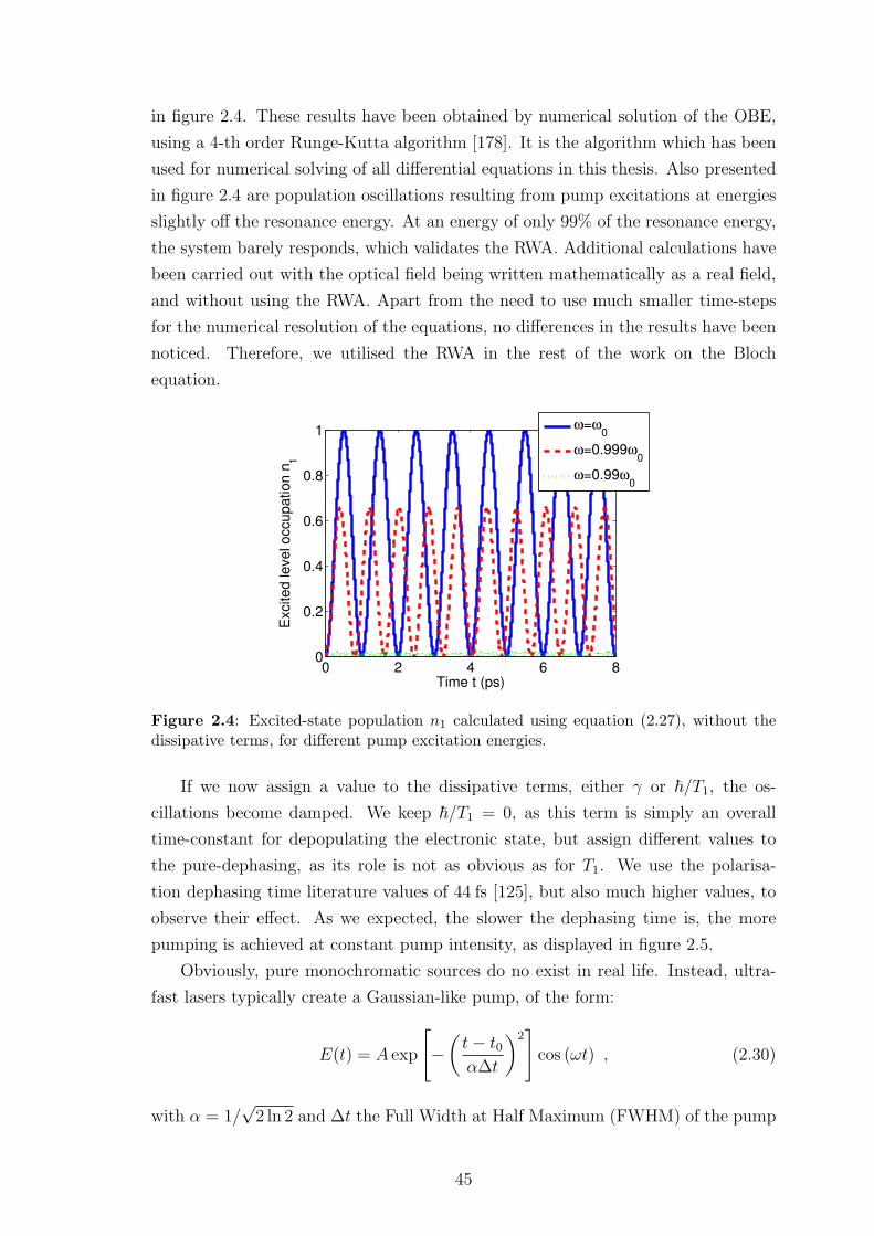
in figure 2.4. These results have been obtained by numerical solution of the OBE,

using a 4-th order Runge-Kutta algorithm [178]. It is the algorithm which has been

used for numerical solving of all differential equations in this thesis. Also presented

in figure 2.4 are population oscillations resulting from pump excitations at energies

slightly off the resonance energy. At an energy of only 99% of the resonance energy,

the system barely responds, which validates the RWA. Additional calculations have

been carried out with the optical field being written mathematically as a real field,

and without using the RWA. Apart from the need to use much smaller time-steps

for the numerical resolution of the equations, no differences in the results have been

noticed. Therefore, we utilised the RWA in the rest of the work on the Bloch

equation.

0 2 4 6 80

0.2

0.4

0.6

0.8

1

Time t (ps)

Excited level occupation n

1

ω=ω0

ω=0.999ω0

ω=0.99ω0

Figure 2.4: Excited-state population n1 calculated using equation (2.27), without thedissipative terms, for different pump excitation energies.

If we now assign a value to the dissipative terms, either γ or ~/T1, the os-

cillations become damped. We keep ~/T1 = 0, as this term is simply an overall

time-constant for depopulating the electronic state, but assign different values to

the pure-dephasing, as its role is not as obvious as for T1. We use the polarisa-

tion dephasing time literature values of 44 fs [125], but also much higher values, to

observe their effect. As we expected, the slower the dephasing time is, the more

pumping is achieved at constant pump intensity, as displayed in figure 2.5.

Obviously, pure monochromatic sources do no exist in real life. Instead, ultra-

fast lasers typically create a Gaussian-like pump, of the form:

E(t) = A exp

[−(t− t0α∆t

)2]cos (ωt) , (2.30)

with α = 1/√2 ln 2 and ∆t the Full Width at Half Maximum (FWHM) of the pump

45

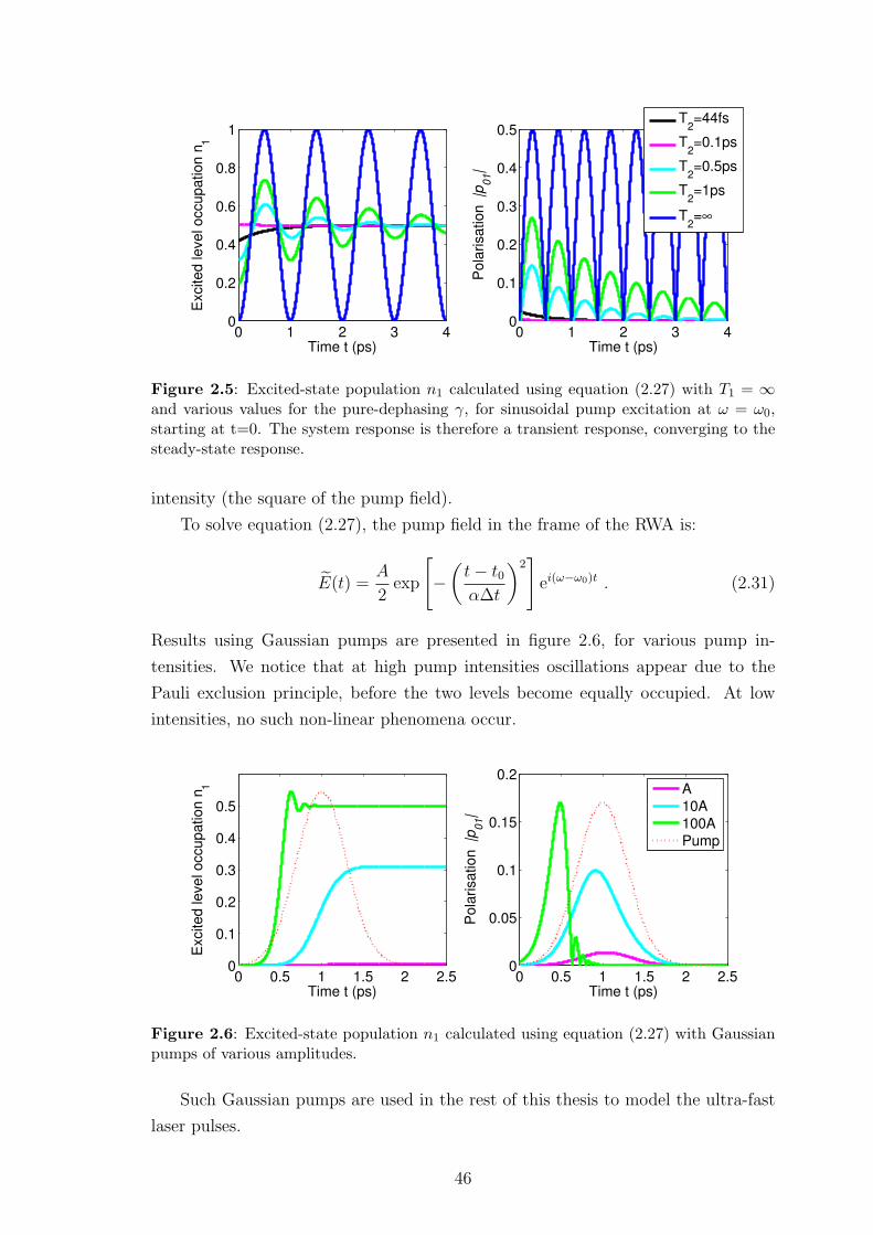
0 1 2 3 40

0.2

0.4

0.6

0.8

1

Time t (ps)

Excited level occupation n

1

0 1 2 3 40

0.1

0.2

0.3

0.4

0.5

Time t (ps)

Pola

risation |p

01|

T

2=44fs

T2=0.1ps

T2=0.5ps

T2=1ps

T2=∞

Figure 2.5: Excited-state population n1 calculated using equation (2.27) with T1 = ∞and various values for the pure-dephasing γ, for sinusoidal pump excitation at ω = ω0,starting at t=0. The system response is therefore a transient response, converging to thesteady-state response.

intensity (the square of the pump field).

To solve equation (2.27), the pump field in the frame of the RWA is:

E(t) =A

2exp

[−(t− t0α∆t

)2]ei(ω−ω0)t . (2.31)

Results using Gaussian pumps are presented in figure 2.6, for various pump in-

tensities. We notice that at high pump intensities oscillations appear due to the

Pauli exclusion principle, before the two levels become equally occupied. At low

intensities, no such non-linear phenomena occur.

0 0.5 1 1.5 2 2.50

0.1

0.2

0.3

0.4

0.5

Time t (ps)

Excited level occupation n

1

0 0.5 1 1.5 2 2.50

0.05

0.1

0.15

0.2

Time t (ps)

Pola

risation |p

01|

A

10A

100A

Pump

Figure 2.6: Excited-state population n1 calculated using equation (2.27) with Gaussianpumps of various amplitudes.

Such Gaussian pumps are used in the rest of this thesis to model the ultra-fast

laser pulses.

46

A single six-level system

A two-level system is certainly not a very realistic model of a chromophore.

Indeed, a chromophore usually possesses numerous excitable (“bright”) electronic

levels, in addition to a multitude of associated vibrational levels [14]. Bright elec-

tronic excited states are usually separated from the ground electronic states by

bandgaps of a few electronvolts (typically 3 eV for polyfluorene) and are similarly

far apart from each other, so that we can neglect any other electronic state that is

not tuned with the pump excitation. However, vibrational levels are usually energet-

ically close to electronic levels (typically 0.1 eV in polyfluorenes) and therefore can

play an important role in the photo-physics of molecules. Schumacher et al. [125]

have shown that, from the point of view of the photo-physics, a 6-level model is a

very good approximation of an oligofluorene molecule. In this part we will show

how the OBE are modified to include six levels instead of only two, and highlight

some particular results of interest.

According to Schumacher et al. [125], the four additional levels to include in the

model correspond to two vibrational levels for each electronic level. The levels of the

same electronic state are dipole forbidden and therefore are not optically coupled, so

that the ground state levels are only optically coupled with the excited states. The

energy of these six levels is taken from the values published by S. Schumacher [125].

It is assumed that the transition dipoles are the same between any vibrational level of

the same electronic state, the corrections to this being given by the Franck-Condon

factors (see below).

A sketch of the system is presented in figure 2.7. The same method as for the

two-level model is used to derive the OBE for this six-level system. The Rotating

Wave Approximation is used as well. As in the previous Subsection, extra empirical

terms have been included in the equations. They are the pure dephasing γdephas,

the vibrational relaxation γrelax and the Franck-Condon factors Fv,v′(n). γrelax is a

term which takes into account the fast-relaxation of excited vibrational states into

the lower electronic state; it therefore depletes the vibrational states to the benefit

of electronic states, and induces dephasing to the polarisation. The Franck-Condon

factors Fv,v′(n) give, for each vibrational mode, the overlap between the vibrational

state v of S0 with the vibrational state v′ of S1 [179]:

Fv,v′(n) = e−β2n2

√v!

v′!βv′−vn Lv′−v

v

(β2n

), (2.32)

with Lv′−vv (β2

n) the Laguerre polynomial:

Lv′−vv

(β2n

)=

v∑

i=max(0,v−v′)

(−1)iv′! (β2n)

i

i!(v − i)!(v′ − v + i)!, (2.33)

47

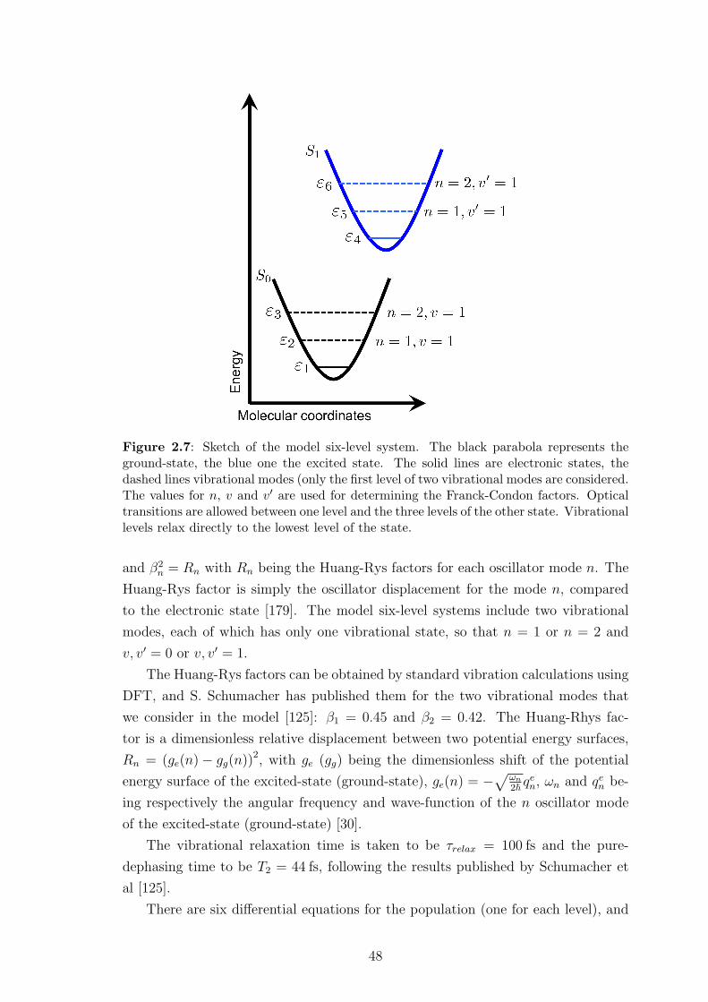
Figure 2.7: Sketch of the model six-level system. The black parabola represents theground-state, the blue one the excited state. The solid lines are electronic states, thedashed lines vibrational modes (only the first level of two vibrational modes are considered.The values for n, v and v′ are used for determining the Franck-Condon factors. Opticaltransitions are allowed between one level and the three levels of the other state. Vibrationallevels relax directly to the lowest level of the state.

and β2n = Rn with Rn being the Huang-Rys factors for each oscillator mode n. The

Huang-Rys factor is simply the oscillator displacement for the mode n, compared

to the electronic state [179]. The model six-level systems include two vibrational

modes, each of which has only one vibrational state, so that n = 1 or n = 2 and

v, v′ = 0 or v, v′ = 1.

The Huang-Rys factors can be obtained by standard vibration calculations using

DFT, and S. Schumacher has published them for the two vibrational modes that

we consider in the model [125]: β1 = 0.45 and β2 = 0.42. The Huang-Rhys fac-

tor is a dimensionless relative displacement between two potential energy surfaces,

Rn = (ge(n)− gg(n))2, with ge (gg) being the dimensionless shift of the potential

energy surface of the excited-state (ground-state), ge(n) = −√

ωn

2~qen, ωn and qen be-

ing respectively the angular frequency and wave-function of the n oscillator mode

of the excited-state (ground-state) [30].

The vibrational relaxation time is taken to be τrelax = 100 fs and the pure-

dephasing time to be T2 = 44 fs, following the results published by Schumacher et

al [125].

There are six differential equations for the population (one for each level), and

48

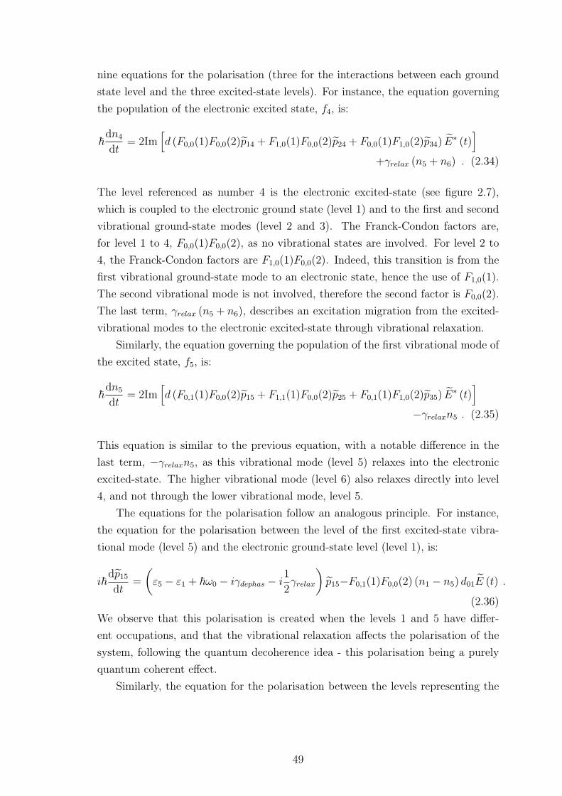
nine equations for the polarisation (three for the interactions between each ground

state level and the three excited-state levels). For instance, the equation governing

the population of the electronic excited state, f4, is:

~dn4

dt= 2Im

[d (F0,0(1)F0,0(2)p14 + F1,0(1)F0,0(2)p24 + F0,0(1)F1,0(2)p34) E

∗ (t)]

+γrelax (n5 + n6) . (2.34)

The level referenced as number 4 is the electronic excited-state (see figure 2.7),

which is coupled to the electronic ground state (level 1) and to the first and second

vibrational ground-state modes (level 2 and 3). The Franck-Condon factors are,

for level 1 to 4, F0,0(1)F0,0(2), as no vibrational states are involved. For level 2 to

4, the Franck-Condon factors are F1,0(1)F0,0(2). Indeed, this transition is from the

first vibrational ground-state mode to an electronic state, hence the use of F1,0(1).

The second vibrational mode is not involved, therefore the second factor is F0,0(2).

The last term, γrelax (n5 + n6), describes an excitation migration from the excited-

vibrational modes to the electronic excited-state through vibrational relaxation.

Similarly, the equation governing the population of the first vibrational mode of

the excited state, f5, is:

~dn5

dt= 2Im

[d (F0,1(1)F0,0(2)p15 + F1,1(1)F0,0(2)p25 + F0,1(1)F1,0(2)p35) E

∗ (t)]

−γrelaxn5 . (2.35)

This equation is similar to the previous equation, with a notable difference in the

last term, −γrelaxn5, as this vibrational mode (level 5) relaxes into the electronic

excited-state. The higher vibrational mode (level 6) also relaxes directly into level

4, and not through the lower vibrational mode, level 5.

The equations for the polarisation follow an analogous principle. For instance,

the equation for the polarisation between the level of the first excited-state vibra-

tional mode (level 5) and the electronic ground-state level (level 1), is:

i~dp15dt

=

(ε5 − ε1 + ~ω0 − iγdephas − i

1

2γrelax

)p15−F0,1(1)F0,0(2) (n1 − n5) d01E (t) .

(2.36)

We observe that this polarisation is created when the levels 1 and 5 have differ-

ent occupations, and that the vibrational relaxation affects the polarisation of the

system, following the quantum decoherence idea - this polarisation being a purely

quantum coherent effect.

Similarly, the equation for the polarisation between the levels representing the

49

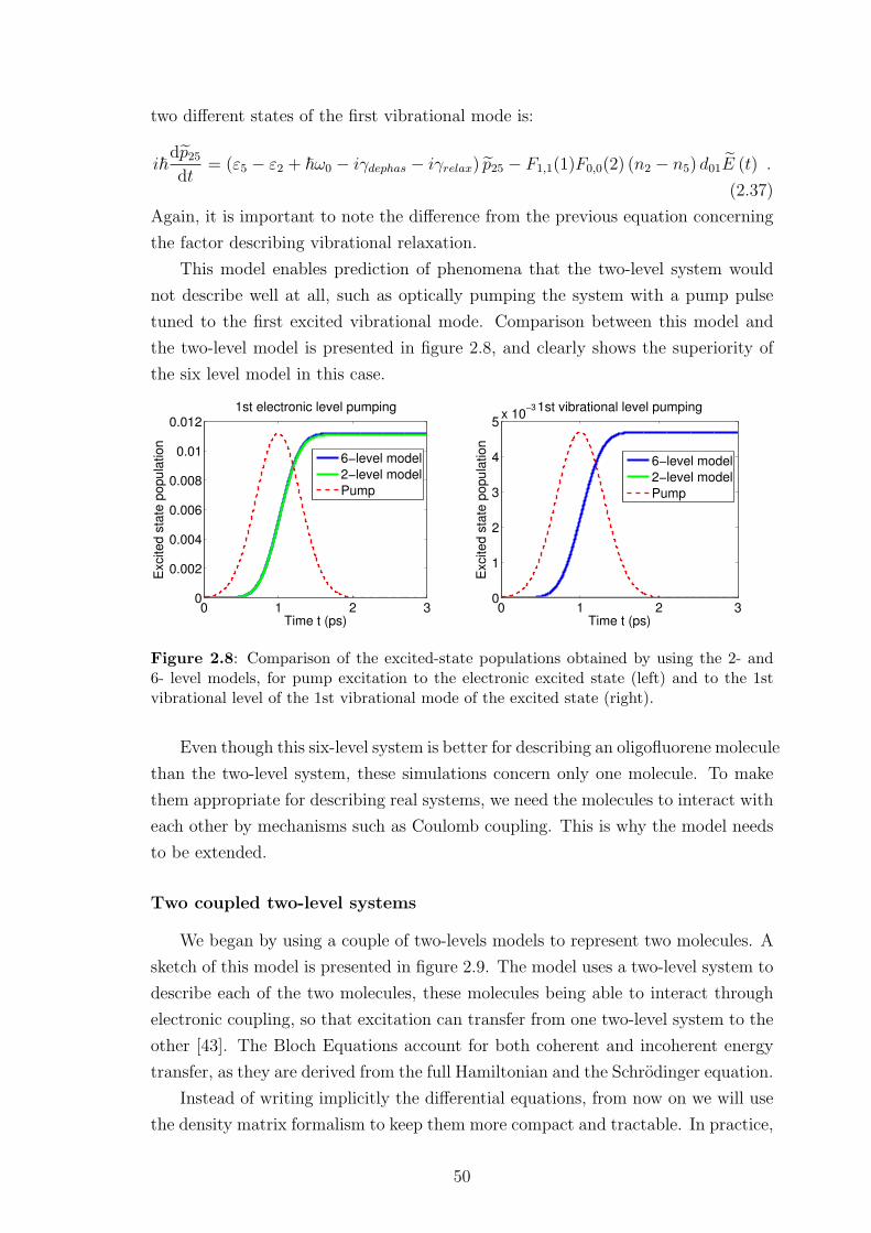
two different states of the first vibrational mode is:

i~dp25dt

= (ε5 − ε2 + ~ω0 − iγdephas − iγrelax) p25 − F1,1(1)F0,0(2) (n2 − n5) d01E (t) .

(2.37)

Again, it is important to note the difference from the previous equation concerning

the factor describing vibrational relaxation.

This model enables prediction of phenomena that the two-level system would

not describe well at all, such as optically pumping the system with a pump pulse

tuned to the first excited vibrational mode. Comparison between this model and

the two-level model is presented in figure 2.8, and clearly shows the superiority of

the six level model in this case.

0 1 2 30

0.002

0.004

0.006

0.008

0.01

0.012

Time t (ps)

Excited s

tate

popula

tion

1st electronic level pumping

6−level model

2−level model

Pump

0 1 2 30

1

2

3

4

5x 10

−3

Time t (ps)

Excited s

tate

popula

tion

1st vibrational level pumping

6−level model

2−level model

Pump

Figure 2.8: Comparison of the excited-state populations obtained by using the 2- and6- level models, for pump excitation to the electronic excited state (left) and to the 1stvibrational level of the 1st vibrational mode of the excited state (right).

Even though this six-level system is better for describing an oligofluorene molecule

than the two-level system, these simulations concern only one molecule. To make

them appropriate for describing real systems, we need the molecules to interact with

each other by mechanisms such as Coulomb coupling. This is why the model needs

to be extended.

Two coupled two-level systems

We began by using a couple of two-levels models to represent two molecules. A

sketch of this model is presented in figure 2.9. The model uses a two-level system to

describe each of the two molecules, these molecules being able to interact through

electronic coupling, so that excitation can transfer from one two-level system to the

other [43]. The Bloch Equations account for both coherent and incoherent energy

transfer, as they are derived from the full Hamiltonian and the Schrodinger equation.

Instead of writing implicitly the differential equations, from now on we will use

the density matrix formalism to keep them more compact and tractable. In practice,

50

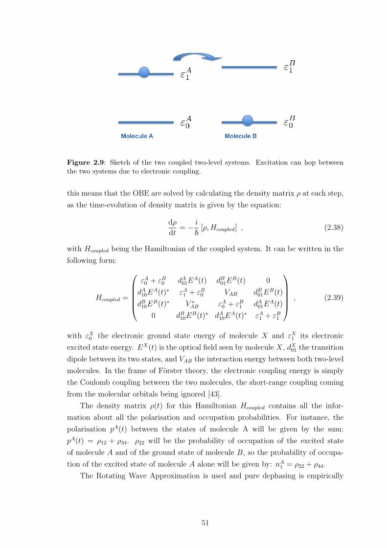
Figure 2.9: Sketch of the two coupled two-level systems. Excitation can hop betweenthe two systems due to electronic coupling.

this means that the OBE are solved by calculating the density matrix ρ at each step,

as the time-evolution of density matrix is given by the equation:

dρ

dt= − i

~[ρ,Hcoupled] , (2.38)

with Hcoupled being the Hamiltonian of the coupled system. It can be written in the

following form:

Hcoupled =

εA0 + εB0 dA01EA(t) dB01E

B(t) 0

dA10EA(t)∗ εA1 + εB0 VAB dB01E

B(t)

dB10EB(t)∗ V ∗

AB εA0 + εB1 dA01EA(t)

0 dB10EB(t)∗ dA10E

A(t)∗ εA1 + εB1

, (2.39)

with εX0 the electronic ground state energy of molecule X and εX1 its electronic

excited state energy. EX(t) is the optical field seen by molecule X, dX01 the transition

dipole between its two states, and VAB the interaction energy between both two-level

molecules. In the frame of Forster theory, the electronic coupling energy is simply

the Coulomb coupling between the two molecules, the short-range coupling coming

from the molecular orbitals being ignored [43].

The density matrix ρ(t) for this Hamiltonian Hcoupled contains all the infor-

mation about all the polarisation and occupation probabilities. For instance, the

polarisation pA(t) between the states of molecule A will be given by the sum:

pA(t) = ρ12 + ρ34. ρ22 will be the probability of occupation of the excited state

of molecule A and of the ground state of molecule B, so the probability of occupa-

tion of the excited state of molecule A alone will be given by: nA1 = ρ22 + ρ44.

The Rotating Wave Approximation is used and pure dephasing is empirically

51

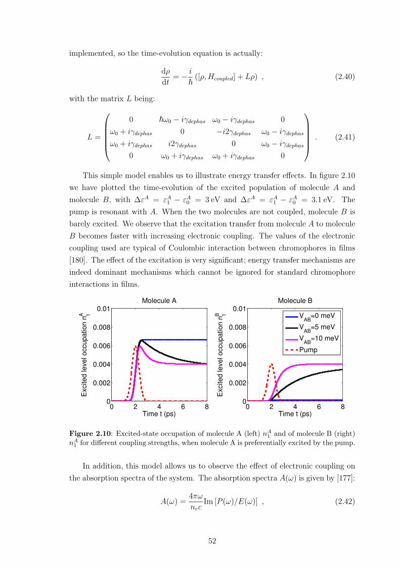
implemented, so the time-evolution equation is actually:

dρ

dt= − i

~([ρ,Hcoupled] + Lρ) , (2.40)

with the matrix L being:

L =

0 ~ω0 − iγdephas ω0 − iγdephas 0

ω0 + iγdephas 0 −i2γdephas ω0 − iγdephas

ω0 + iγdephas i2γdephas 0 ω0 − iγdephas

0 ω0 + iγdephas ω0 + iγdephas 0

. (2.41)

This simple model enables us to illustrate energy transfer effects. In figure 2.10

we have plotted the time-evolution of the excited population of molecule A and

molecule B, with ∆εA = εA1 − εA0 = 3 eV and ∆εA = εA1 − εA0 = 3.1 eV. The

pump is resonant with A. When the two molecules are not coupled, molecule B is

barely excited. We observe that the excitation transfer from molecule A to molecule

B becomes faster with increasing electronic coupling. The values of the electronic

coupling used are typical of Coulombic interaction between chromophores in films

[180]. The effect of the excitation is very significant; energy transfer mechanisms are

indeed dominant mechanisms which cannot be ignored for standard chromophore

interactions in films.

0 2 4 6 80

0.002

0.004

0.006

0.008

0.01

Time t (ps)

Excited level occupation n

1A

Molecule A

0 2 4 6 80

0.002

0.004

0.006

0.008

0.01

Time t (ps)

Excited level occupation n

1B

Molecule B

VAB

=0 meV

VAB

=5 meV

VAB

=10 meV

Pump

Figure 2.10: Excited-state occupation of molecule A (left) nA1 and of molecule B (right)

nA1 for different coupling strengths, when molecule A is preferentially excited by the pump.

In addition, this model allows us to observe the effect of electronic coupling on

the absorption spectra of the system. The absorption spectra A(ω) is given by [177]:

A(ω) =4πω

nrcIm [P (ω)/E(ω)] , (2.42)

52

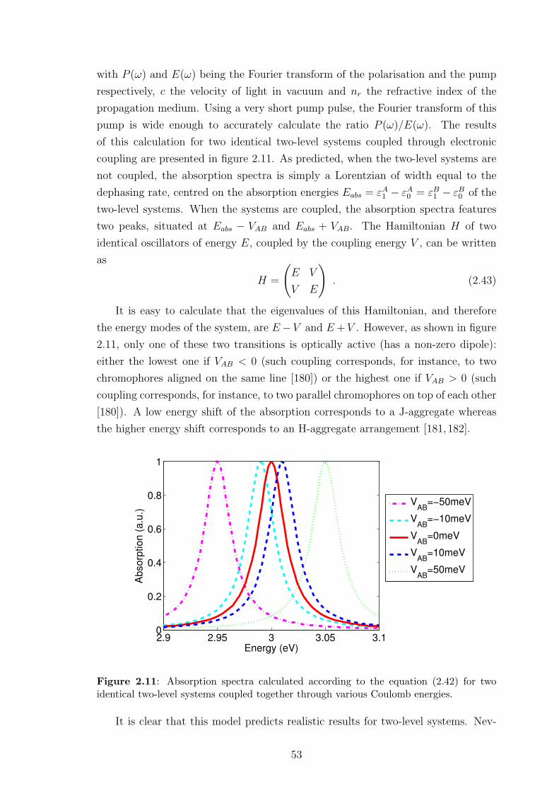
with P (ω) and E(ω) being the Fourier transform of the polarisation and the pump

respectively, c the velocity of light in vacuum and nr the refractive index of the

propagation medium. Using a very short pump pulse, the Fourier transform of this

pump is wide enough to accurately calculate the ratio P (ω)/E(ω). The results

of this calculation for two identical two-level systems coupled through electronic

coupling are presented in figure 2.11. As predicted, when the two-level systems are

not coupled, the absorption spectra is simply a Lorentzian of width equal to the

dephasing rate, centred on the absorption energies Eabs = εA1 − εA0 = εB1 − εB0 of the

two-level systems. When the systems are coupled, the absorption spectra features

two peaks, situated at Eabs − VAB and Eabs + VAB. The Hamiltonian H of two

identical oscillators of energy E, coupled by the coupling energy V , can be written

as

H =

(E V

V E

). (2.43)

It is easy to calculate that the eigenvalues of this Hamiltonian, and therefore

the energy modes of the system, are E−V and E+V . However, as shown in figure

2.11, only one of these two transitions is optically active (has a non-zero dipole):

either the lowest one if VAB < 0 (such coupling corresponds, for instance, to two

chromophores aligned on the same line [180]) or the highest one if VAB > 0 (such

coupling corresponds, for instance, to two parallel chromophores on top of each other

[180]). A low energy shift of the absorption corresponds to a J-aggregate whereas

the higher energy shift corresponds to an H-aggregate arrangement [181,182].

2.9 2.95 3 3.05 3.10

0.2

0.4

0.6

0.8

1

Energy (eV)

Ab

so

rptio

n (

a.u

.)

VAB

=−50meV

VAB

=−10meV

VAB

=0meV

VAB

=10meV

VAB

=50meV

Figure 2.11: Absorption spectra calculated according to the equation (2.42) for twoidentical two-level systems coupled together through various Coulomb energies.

It is clear that this model predicts realistic results for two-level systems. Nev-

53

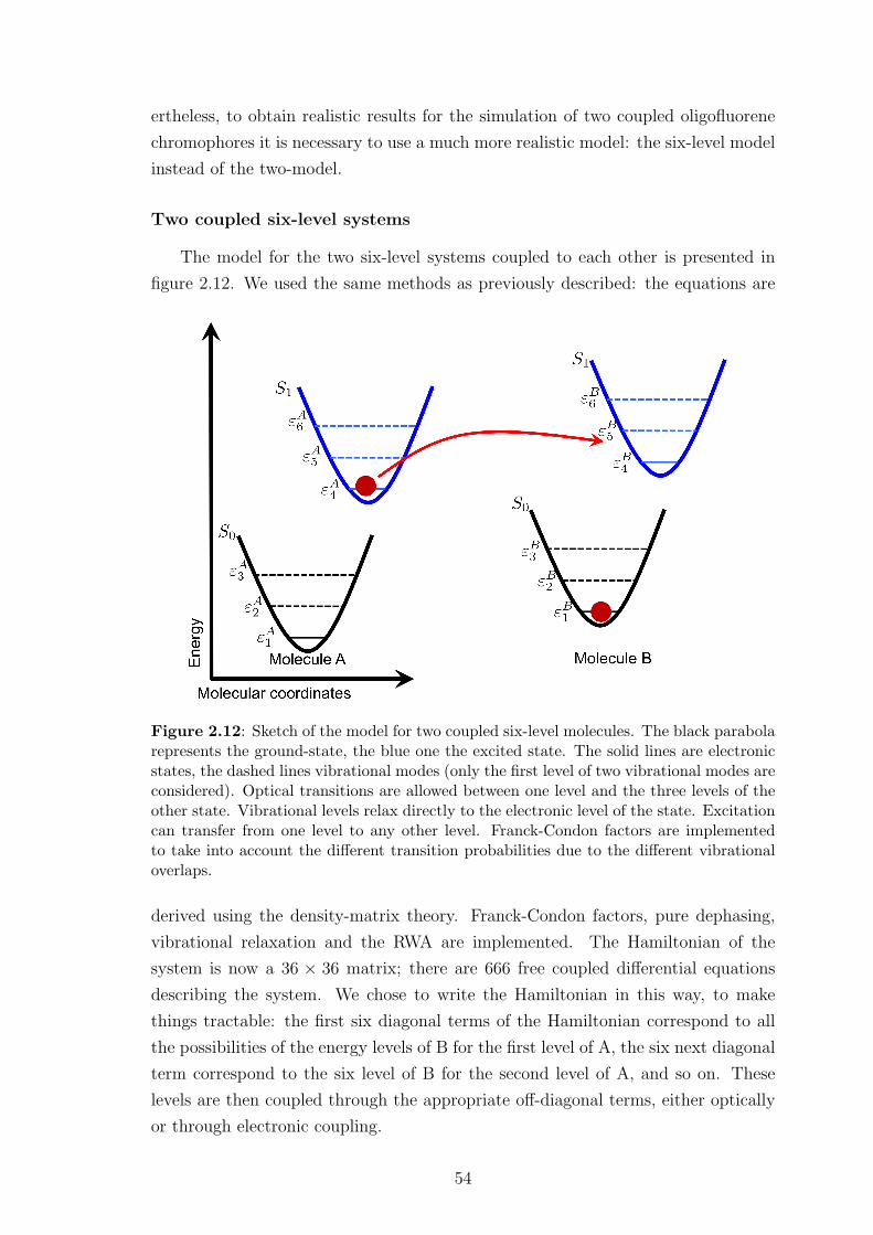
ertheless, to obtain realistic results for the simulation of two coupled oligofluorene

chromophores it is necessary to use a much more realistic model: the six-level model

instead of the two-model.

Two coupled six-level systems

The model for the two six-level systems coupled to each other is presented in

figure 2.12. We used the same methods as previously described: the equations are

Figure 2.12: Sketch of the model for two coupled six-level molecules. The black parabolarepresents the ground-state, the blue one the excited state. The solid lines are electronicstates, the dashed lines vibrational modes (only the first level of two vibrational modes areconsidered). Optical transitions are allowed between one level and the three levels of theother state. Vibrational levels relax directly to the electronic level of the state. Excitationcan transfer from one level to any other level. Franck-Condon factors are implementedto take into account the different transition probabilities due to the different vibrationaloverlaps.

derived using the density-matrix theory. Franck-Condon factors, pure dephasing,

vibrational relaxation and the RWA are implemented. The Hamiltonian of the

system is now a 36 × 36 matrix; there are 666 free coupled differential equations

describing the system. We chose to write the Hamiltonian in this way, to make

things tractable: the first six diagonal terms of the Hamiltonian correspond to all

the possibilities of the energy levels of B for the first level of A, the six next diagonal

term correspond to the six level of B for the second level of A, and so on. These

levels are then coupled through the appropriate off-diagonal terms, either optically

or through electronic coupling.

54

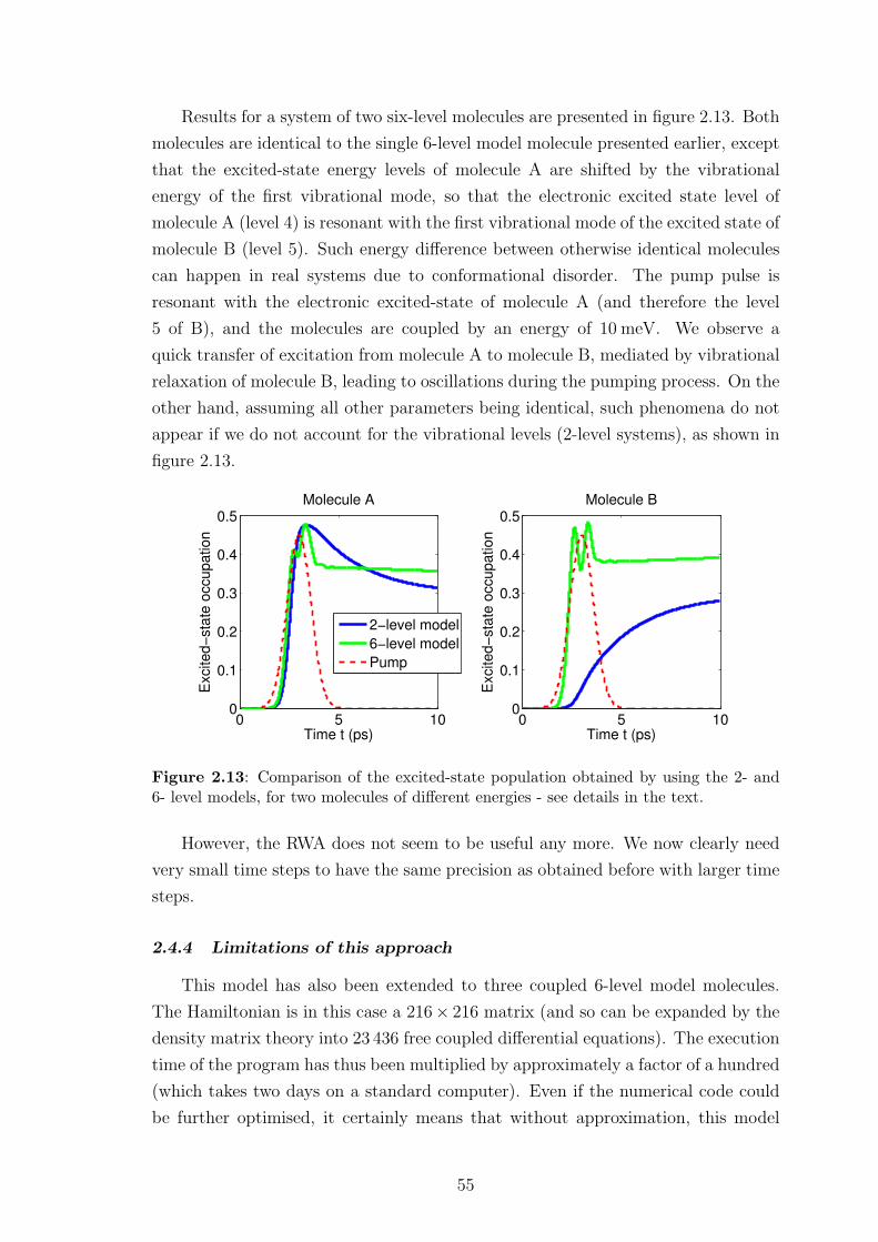
Results for a system of two six-level molecules are presented in figure 2.13. Both

molecules are identical to the single 6-level model molecule presented earlier, except

that the excited-state energy levels of molecule A are shifted by the vibrational

energy of the first vibrational mode, so that the electronic excited state level of

molecule A (level 4) is resonant with the first vibrational mode of the excited state of

molecule B (level 5). Such energy difference between otherwise identical molecules

can happen in real systems due to conformational disorder. The pump pulse is

resonant with the electronic excited-state of molecule A (and therefore the level

5 of B), and the molecules are coupled by an energy of 10 meV. We observe a

quick transfer of excitation from molecule A to molecule B, mediated by vibrational

relaxation of molecule B, leading to oscillations during the pumping process. On the

other hand, assuming all other parameters being identical, such phenomena do not

appear if we do not account for the vibrational levels (2-level systems), as shown in

figure 2.13.

0 5 100

0.1

0.2

0.3

0.4

0.5

Time t (ps)

Excited−

sta

te o

ccupation

Molecule A

0 5 100

0.1

0.2

0.3

0.4

0.5

Time t (ps)

Excited−

sta

te o

ccupation

Molecule B

2−level model

6−level model

Pump

Figure 2.13: Comparison of the excited-state population obtained by using the 2- and6- level models, for two molecules of different energies - see details in the text.

However, the RWA does not seem to be useful any more. We now clearly need

very small time steps to have the same precision as obtained before with larger time

steps.

2.4.4 Limitations of this approach

This model has also been extended to three coupled 6-level model molecules.

The Hamiltonian is in this case a 216× 216 matrix (and so can be expanded by the

density matrix theory into 23 436 free coupled differential equations). The execution

time of the program has thus been multiplied by approximately a factor of a hundred

(which takes two days on a standard computer). Even if the numerical code could

be further optimised, it certainly means that without approximation, this model

55

could not be extended to four molecules. In term of memory, limits would also be

reached quickly.

Real systems are typically made of 1023 (Avogadro’s number) chromophores,

and each chromophore interacts with tens of other chromophores. It is therefore

impossible to extend the formalism of the Optical Bloch Equations to a real-life

system. However, these results constitute the basics of a development of a simplified,

but yet accurate model to predict the excitation dynamics of real-life system. It will

be presented in the last Chapter of this thesis.

2.5 Conclusion

In this Chapter, we have detailed the methods that we are going to use in

the rest of this thesis, in order to gain knowledge about ultra-fast photo-physics

of fluorene-based straight and star-shaped molecules. We have chosen to perform

quantum chemistry calculation by the means of DFT, at the B3LYP 6-31G level

of theory (unless specified otherwise), in order to learn about the single ground-

and excited-state properties of the fluorene-based molecules we investigated. Such

excited-state properties are useful to describe molecular relaxation, and therefore

exciton transfer, in star-shaped molecules. This will be demonstrated in Chapters

3 and 4. Single molecule properties, such as transition energy and dipoles, are also

necessary to calculate the inter-molecular interactions playing a major role in the

photo-physics of a large molecular ensemble. This will be discussed in Chapter 5

where some molecular interaction models will be investigated and improved, leading

to the complex large-scale energy transfer dynamics model presented in Chapter 6.

This model will be based on the OBE we have presented here, and will describe the

exciton dynamics arising from interactions between numerous multi-level systems.

Indeed in this Chapter we have shown the importance of interactions between multi-

level systems in accurately describing the ultra-fast photo-physics processes, such as

exciton transfer, between oligofluorene molecules.

56

Chapter 3

Optical properties of fluorene-based C3-symmetric

molecules

In this Chapter, we present a detailed combined experimental and theoretical

study of the low energy optical transitions in two families of star-shaped molecules.

Both families have three-fold rotational symmetry (“C3-symmetry”) with oligoflu-

orene arms attached to a central core. This study of the fundamental optical and

electronic properties of these star-shaped molecules is essential if one wants to under-

stand the mechanisms of exciton transfer in these branched molecules. The results

presented in this Chapter are necessary to gain detailed knowledge of intra-molecular

exciton transfer in this family of molecules, which will be presented in Chapter 4.

3.1 Background: why are star-shaped molecules important?

As highlighted in Chapter 1, the most widely studied solution-processable, or-

ganic semiconducting materials are conjugated polymers. However, we have also

seen that several other small molecular geometries can be utilised, including den-

drimers [183], spiro-compounds [184] and star-shaped molecules [185]. The influence

of the shape of the molecules on their light absorption and emission properties is

therefore an important issue if one wants to design new and efficient devices with

these less known materials. Star-shaped molecules also make for an excellent model

system to study intra-molecular exciton transfer because, contrary to polymers, their

geometry is known accurately in solution, and is therefore of particular interest in

our studies.

Star-shaped molecules have several advantages over the established polymer

materials such as no polydispersity, increased solubility and improved morphology

in films. This results in overall easier experimental processing. They have been

shown to exhibit many desirable properties such as high solid state photolumines-

cence quantum yield (PLQY) or high non-linear absorption coefficients [82,186–190].

Nevertheless, despite increasing interest in star-shaped molecules for technological

purposes, little has been done to understand how their shape influences their pho-

tophysical properties, and previous experimental studies of truxene-cored molecules

have been limited to basic spectral properties [191]. Compared to straight polymer

chains with no particular symmetry, star-shaped molecules possess a C3 point-group

symmetry, making their photo-physics more complex. The one previous theoreti-

57

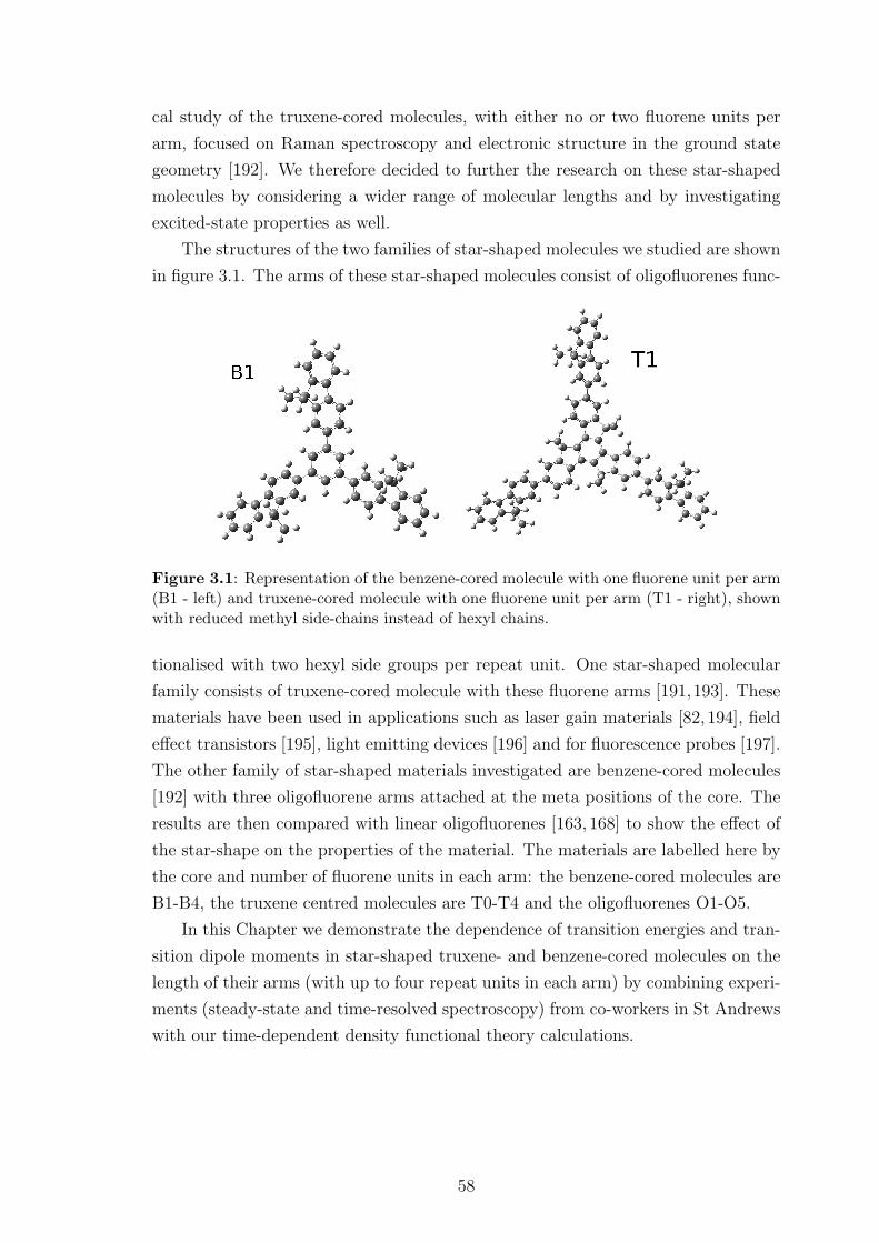
cal study of the truxene-cored molecules, with either no or two fluorene units per

arm, focused on Raman spectroscopy and electronic structure in the ground state

geometry [192]. We therefore decided to further the research on these star-shaped

molecules by considering a wider range of molecular lengths and by investigating

excited-state properties as well.

The structures of the two families of star-shaped molecules we studied are shown

in figure 3.1. The arms of these star-shaped molecules consist of oligofluorenes func-

Figure 3.1: Representation of the benzene-cored molecule with one fluorene unit per arm(B1 - left) and truxene-cored molecule with one fluorene unit per arm (T1 - right), shownwith reduced methyl side-chains instead of hexyl chains.

tionalised with two hexyl side groups per repeat unit. One star-shaped molecular

family consists of truxene-cored molecule with these fluorene arms [191,193]. These

materials have been used in applications such as laser gain materials [82, 194], field

effect transistors [195], light emitting devices [196] and for fluorescence probes [197].

The other family of star-shaped materials investigated are benzene-cored molecules

[192] with three oligofluorene arms attached at the meta positions of the core. The

results are then compared with linear oligofluorenes [163, 168] to show the effect of

the star-shape on the properties of the material. The materials are labelled here by

the core and number of fluorene units in each arm: the benzene-cored molecules are

B1-B4, the truxene centred molecules are T0-T4 and the oligofluorenes O1-O5.

In this Chapter we demonstrate the dependence of transition energies and tran-

sition dipole moments in star-shaped truxene- and benzene-cored molecules on the

length of their arms (with up to four repeat units in each arm) by combining experi-

ments (steady-state and time-resolved spectroscopy) from co-workers in St Andrews

with our time-dependent density functional theory calculations.

58

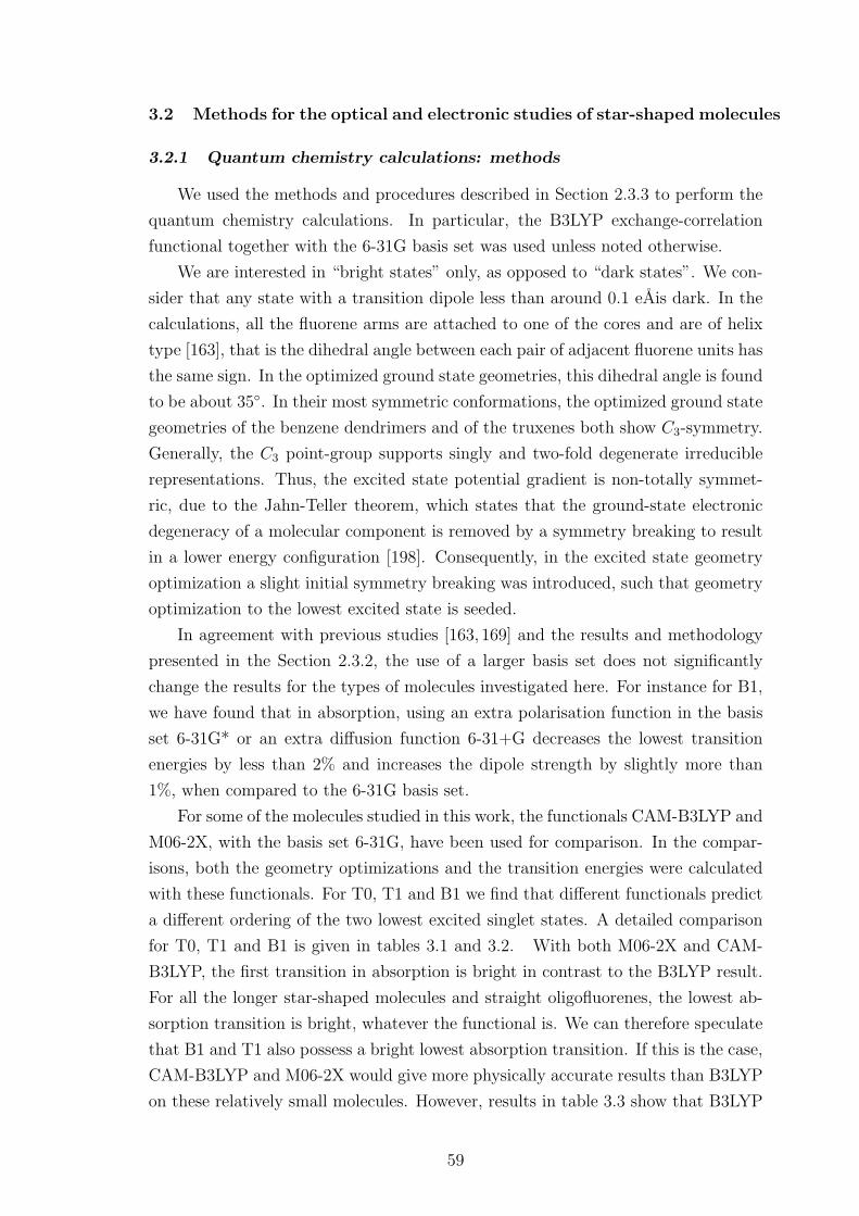
3.2 Methods for the optical and electronic studies of star-shaped molecules

3.2.1 Quantum chemistry calculations: methods

We used the methods and procedures described in Section 2.3.3 to perform the

quantum chemistry calculations. In particular, the B3LYP exchange-correlation

functional together with the 6-31G basis set was used unless noted otherwise.

We are interested in “bright states” only, as opposed to “dark states”. We con-

sider that any state with a transition dipole less than around 0.1 eAis dark. In the

calculations, all the fluorene arms are attached to one of the cores and are of helix

type [163], that is the dihedral angle between each pair of adjacent fluorene units has

the same sign. In the optimized ground state geometries, this dihedral angle is found

to be about 35. In their most symmetric conformations, the optimized ground state

geometries of the benzene dendrimers and of the truxenes both show C3-symmetry.

Generally, the C3 point-group supports singly and two-fold degenerate irreducible

representations. Thus, the excited state potential gradient is non-totally symmet-

ric, due to the Jahn-Teller theorem, which states that the ground-state electronic

degeneracy of a molecular component is removed by a symmetry breaking to result

in a lower energy configuration [198]. Consequently, in the excited state geometry

optimization a slight initial symmetry breaking was introduced, such that geometry

optimization to the lowest excited state is seeded.

In agreement with previous studies [163, 169] and the results and methodology

presented in the Section 2.3.2, the use of a larger basis set does not significantly

change the results for the types of molecules investigated here. For instance for B1,

we have found that in absorption, using an extra polarisation function in the basis

set 6-31G* or an extra diffusion function 6-31+G decreases the lowest transition

energies by less than 2% and increases the dipole strength by slightly more than

1%, when compared to the 6-31G basis set.

For some of the molecules studied in this work, the functionals CAM-B3LYP and

M06-2X, with the basis set 6-31G, have been used for comparison. In the compar-

isons, both the geometry optimizations and the transition energies were calculated

with these functionals. For T0, T1 and B1 we find that different functionals predict

a different ordering of the two lowest excited singlet states. A detailed comparison

for T0, T1 and B1 is given in tables 3.1 and 3.2. With both M06-2X and CAM-

B3LYP, the first transition in absorption is bright in contrast to the B3LYP result.

For all the longer star-shaped molecules and straight oligofluorenes, the lowest ab-

sorption transition is bright, whatever the functional is. We can therefore speculate

that B1 and T1 also possess a bright lowest absorption transition. If this is the case,

CAM-B3LYP and M06-2X would give more physically accurate results than B3LYP

on these relatively small molecules. However, results in table 3.3 show that B3LYP

59

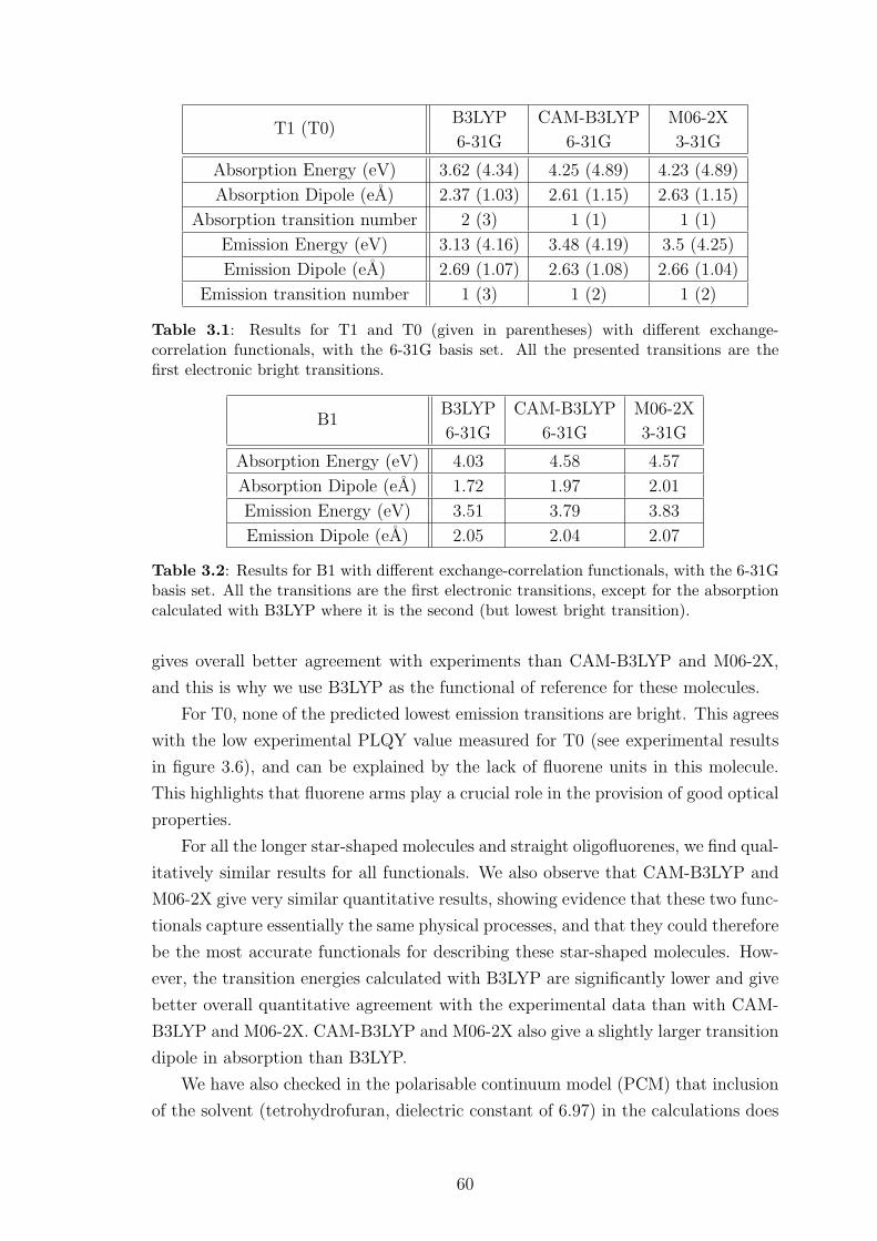
T1 (T0)B3LYP

6-31G

CAM-B3LYP

6-31G

M06-2X

3-31G

Absorption Energy (eV) 3.62 (4.34) 4.25 (4.89) 4.23 (4.89)

Absorption Dipole (eA) 2.37 (1.03) 2.61 (1.15) 2.63 (1.15)

Absorption transition number 2 (3) 1 (1) 1 (1)

Emission Energy (eV) 3.13 (4.16) 3.48 (4.19) 3.5 (4.25)

Emission Dipole (eA) 2.69 (1.07) 2.63 (1.08) 2.66 (1.04)

Emission transition number 1 (3) 1 (2) 1 (2)

Table 3.1: Results for T1 and T0 (given in parentheses) with different exchange-correlation functionals, with the 6-31G basis set. All the presented transitions are thefirst electronic bright transitions.

B1B3LYP

6-31G

CAM-B3LYP

6-31G

M06-2X

3-31G

Absorption Energy (eV) 4.03 4.58 4.57

Absorption Dipole (eA) 1.72 1.97 2.01

Emission Energy (eV) 3.51 3.79 3.83

Emission Dipole (eA) 2.05 2.04 2.07

Table 3.2: Results for B1 with different exchange-correlation functionals, with the 6-31Gbasis set. All the transitions are the first electronic transitions, except for the absorptioncalculated with B3LYP where it is the second (but lowest bright transition).

gives overall better agreement with experiments than CAM-B3LYP and M06-2X,

and this is why we use B3LYP as the functional of reference for these molecules.

For T0, none of the predicted lowest emission transitions are bright. This agrees

with the low experimental PLQY value measured for T0 (see experimental results

in figure 3.6), and can be explained by the lack of fluorene units in this molecule.

This highlights that fluorene arms play a crucial role in the provision of good optical

properties.

For all the longer star-shaped molecules and straight oligofluorenes, we find qual-

itatively similar results for all functionals. We also observe that CAM-B3LYP and

M06-2X give very similar quantitative results, showing evidence that these two func-

tionals capture essentially the same physical processes, and that they could therefore

be the most accurate functionals for describing these star-shaped molecules. How-

ever, the transition energies calculated with B3LYP are significantly lower and give

better overall quantitative agreement with the experimental data than with CAM-

B3LYP and M06-2X. CAM-B3LYP and M06-2X also give a slightly larger transition

dipole in absorption than B3LYP.

We have also checked in the polarisable continuum model (PCM) that inclusion

of the solvent (tetrohydrofuran, dielectric constant of 6.97) in the calculations does

60

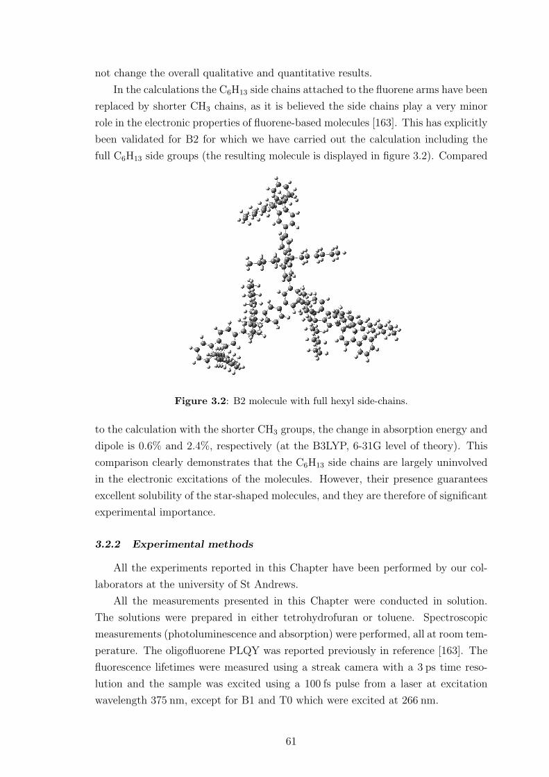
not change the overall qualitative and quantitative results.

In the calculations the C6H13 side chains attached to the fluorene arms have been

replaced by shorter CH3 chains, as it is believed the side chains play a very minor

role in the electronic properties of fluorene-based molecules [163]. This has explicitly

been validated for B2 for which we have carried out the calculation including the

full C6H13 side groups (the resulting molecule is displayed in figure 3.2). Compared

Figure 3.2: B2 molecule with full hexyl side-chains.

to the calculation with the shorter CH3 groups, the change in absorption energy and

dipole is 0.6% and 2.4%, respectively (at the B3LYP, 6-31G level of theory). This

comparison clearly demonstrates that the C6H13 side chains are largely uninvolved

in the electronic excitations of the molecules. However, their presence guarantees

excellent solubility of the star-shaped molecules, and they are therefore of significant

experimental importance.

3.2.2 Experimental methods

All the experiments reported in this Chapter have been performed by our col-

laborators at the university of St Andrews.

All the measurements presented in this Chapter were conducted in solution.

The solutions were prepared in either tetrohydrofuran or toluene. Spectroscopic

measurements (photoluminescence and absorption) were performed, all at room tem-

perature. The oligofluorene PLQY was reported previously in reference [163]. The

fluorescence lifetimes were measured using a streak camera with a 3 ps time reso-

lution and the sample was excited using a 100 fs pulse from a laser at excitation

wavelength 375 nm, except for B1 and T0 which were excited at 266 nm.

61

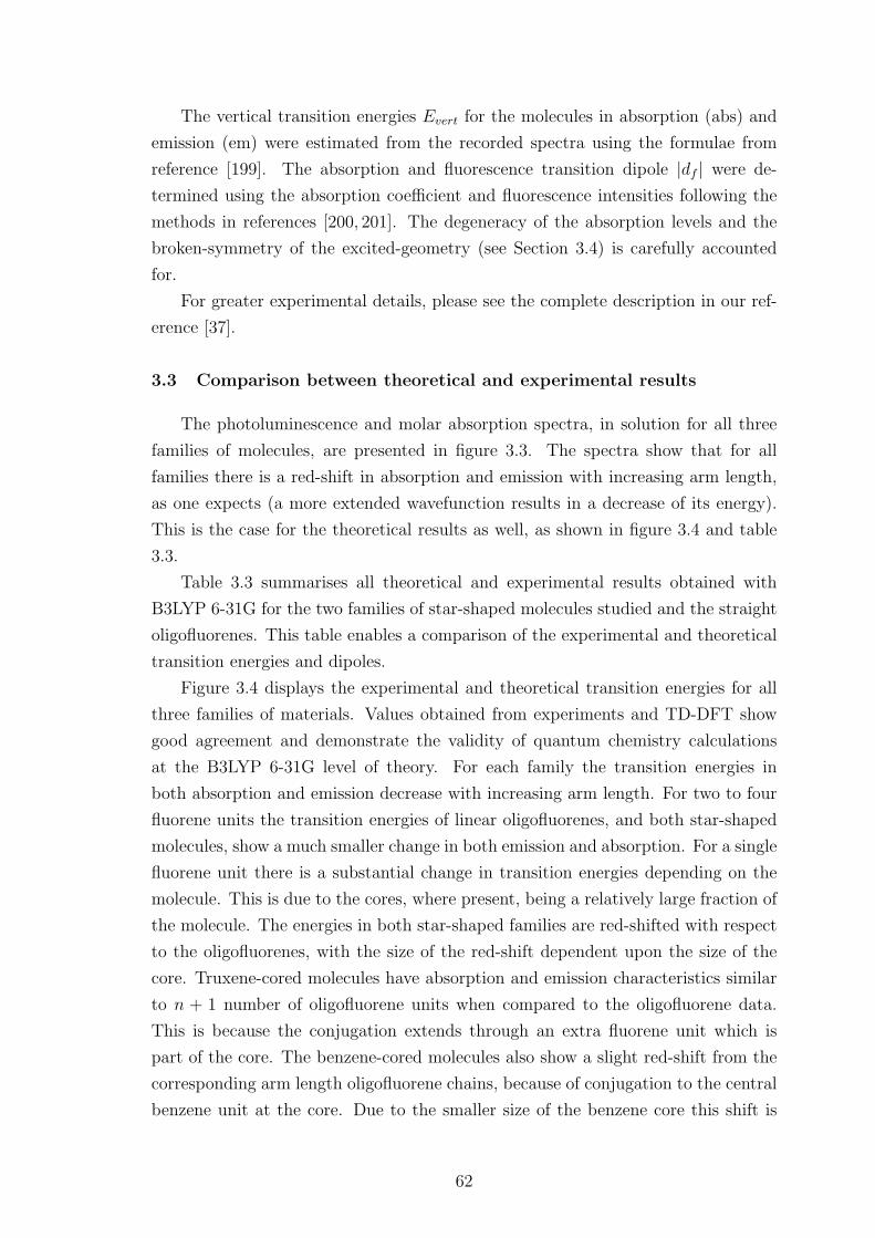
The vertical transition energies Evert for the molecules in absorption (abs) and

emission (em) were estimated from the recorded spectra using the formulae from

reference [199]. The absorption and fluorescence transition dipole |df | were de-

termined using the absorption coefficient and fluorescence intensities following the

methods in references [200, 201]. The degeneracy of the absorption levels and the

broken-symmetry of the excited-geometry (see Section 3.4) is carefully accounted

for.

For greater experimental details, please see the complete description in our ref-

erence [37].

3.3 Comparison between theoretical and experimental results

The photoluminescence and molar absorption spectra, in solution for all three

families of molecules, are presented in figure 3.3. The spectra show that for all

families there is a red-shift in absorption and emission with increasing arm length,

as one expects (a more extended wavefunction results in a decrease of its energy).

This is the case for the theoretical results as well, as shown in figure 3.4 and table

3.3.

Table 3.3 summarises all theoretical and experimental results obtained with

B3LYP 6-31G for the two families of star-shaped molecules studied and the straight

oligofluorenes. This table enables a comparison of the experimental and theoretical

transition energies and dipoles.

Figure 3.4 displays the experimental and theoretical transition energies for all

three families of materials. Values obtained from experiments and TD-DFT show

good agreement and demonstrate the validity of quantum chemistry calculations

at the B3LYP 6-31G level of theory. For each family the transition energies in

both absorption and emission decrease with increasing arm length. For two to four

fluorene units the transition energies of linear oligofluorenes, and both star-shaped

molecules, show a much smaller change in both emission and absorption. For a single

fluorene unit there is a substantial change in transition energies depending on the

molecule. This is due to the cores, where present, being a relatively large fraction of

the molecule. The energies in both star-shaped families are red-shifted with respect

to the oligofluorenes, with the size of the red-shift dependent upon the size of the

core. Truxene-cored molecules have absorption and emission characteristics similar

to n + 1 number of oligofluorene units when compared to the oligofluorene data.

This is because the conjugation extends through an extra fluorene unit which is

part of the core. The benzene-cored molecules also show a slight red-shift from the

corresponding arm length oligofluorene chains, because of conjugation to the central

benzene unit at the core. Due to the smaller size of the benzene core this shift is

62

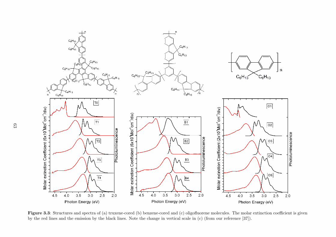
Figure 3.3: Structures and spectra of (a) truxene-cored (b) benzene-cored and (c) oligofluorene molecules. The molar extinction coefficient is givenby the red lines and the emission by the black lines. Note the change in vertical scale in (c) (from our reference [37]).

63

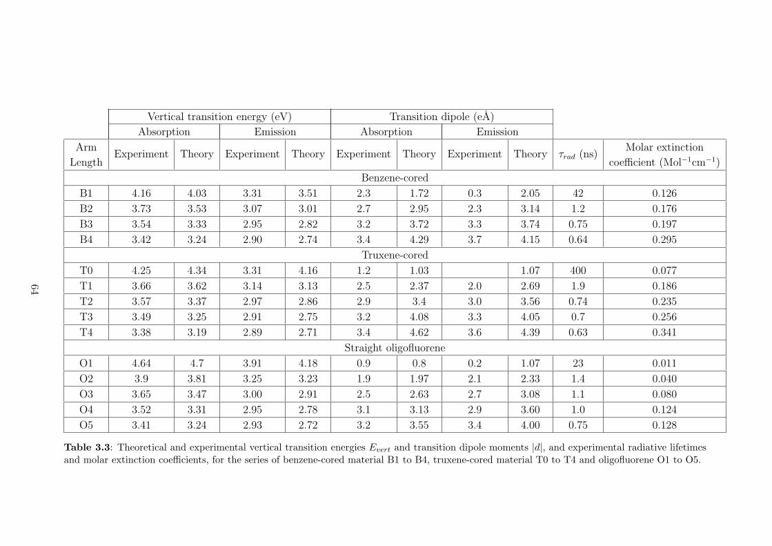
Vertical transition energy (eV) Transition dipole (eA)

Absorption Emission Absorption Emission

Arm

LengthExperiment Theory Experiment Theory Experiment Theory Experiment Theory τrad (ns)

Molar extinction

coefficient (Mol−1cm−1)

Benzene-cored

B1 4.16 4.03 3.31 3.51 2.3 1.72 0.3 2.05 42 0.126

B2 3.73 3.53 3.07 3.01 2.7 2.95 2.3 3.14 1.2 0.176

B3 3.54 3.33 2.95 2.82 3.2 3.72 3.3 3.74 0.75 0.197

B4 3.42 3.24 2.90 2.74 3.4 4.29 3.7 4.15 0.64 0.295

Truxene-cored

T0 4.25 4.34 3.31 4.16 1.2 1.03 1.07 400 0.077

T1 3.66 3.62 3.14 3.13 2.5 2.37 2.0 2.69 1.9 0.186

T2 3.57 3.37 2.97 2.86 2.9 3.4 3.0 3.56 0.74 0.235

T3 3.49 3.25 2.91 2.75 3.2 4.08 3.3 4.05 0.7 0.256

T4 3.38 3.19 2.89 2.71 3.4 4.62 3.6 4.39 0.63 0.341

Straight oligofluorene

O1 4.64 4.7 3.91 4.18 0.9 0.8 0.2 1.07 23 0.011

O2 3.9 3.81 3.25 3.23 1.9 1.97 2.1 2.33 1.4 0.040

O3 3.65 3.47 3.00 2.91 2.5 2.63 2.7 3.08 1.1 0.080

O4 3.52 3.31 2.95 2.78 3.1 3.13 2.9 3.60 1.0 0.124

O5 3.41 3.24 2.93 2.72 3.2 3.55 3.4 4.00 0.75 0.128

Table 3.3: Theoretical and experimental vertical transition energies Evert and transition dipole moments |d|, and experimental radiative lifetimesand molar extinction coefficients, for the series of benzene-cored material B1 to B4, truxene-cored material T0 to T4 and oligofluorene O1 to O5.

64

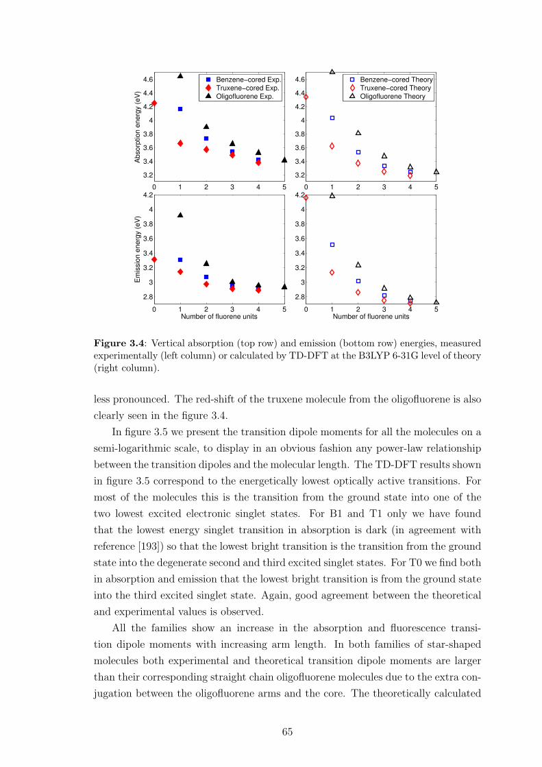
0 1 2 3 4 5

3.2

3.4

3.6

3.8

4

4.2

4.4

4.6

Ab

so

rptio

n e

ne

rgy (

eV

)

Benzene−cored Exp.Truxene−cored Exp.Oligofluorene Exp.

0 1 2 3 4 5

3.2

3.4

3.6

3.8

4

4.2

4.4

4.6

Benzene−cored TheoryTruxene−cored TheoryOligofluorene Theory

0 1 2 3 4 5

2.8

3

3.2

3.4

3.6

3.8

4

4.2

Em

issio

n e

ne

rgy (

eV

)

Number of fluorene units0 1 2 3 4 5

2.8

3

3.2

3.4

3.6

3.8

4

4.2

Number of fluorene units

Figure 3.4: Vertical absorption (top row) and emission (bottom row) energies, measuredexperimentally (left column) or calculated by TD-DFT at the B3LYP 6-31G level of theory(right column).

less pronounced. The red-shift of the truxene molecule from the oligofluorene is also

clearly seen in the figure 3.4.

In figure 3.5 we present the transition dipole moments for all the molecules on a

semi-logarithmic scale, to display in an obvious fashion any power-law relationship

between the transition dipoles and the molecular length. The TD-DFT results shown

in figure 3.5 correspond to the energetically lowest optically active transitions. For

most of the molecules this is the transition from the ground state into one of the

two lowest excited electronic singlet states. For B1 and T1 only we have found

that the lowest energy singlet transition in absorption is dark (in agreement with

reference [193]) so that the lowest bright transition is the transition from the ground

state into the degenerate second and third excited singlet states. For T0 we find both

in absorption and emission that the lowest bright transition is from the ground state

into the third excited singlet state. Again, good agreement between the theoretical

and experimental values is observed.

All the families show an increase in the absorption and fluorescence transi-

tion dipole moments with increasing arm length. In both families of star-shaped

molecules both experimental and theoretical transition dipole moments are larger

than their corresponding straight chain oligofluorene molecules due to the extra con-

jugation between the oligofluorene arms and the core. The theoretically calculated

65

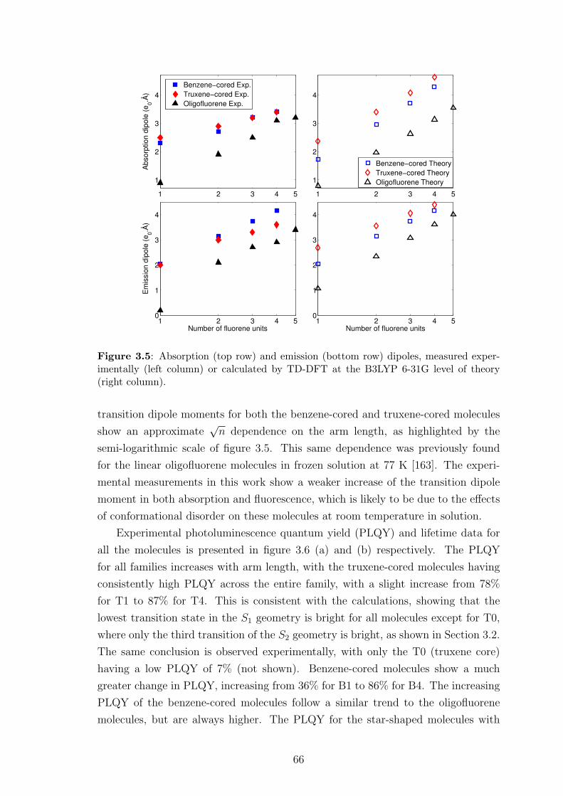
1 2 3 4 5

1

2

3

4

Abs

orpt

ion

dipo

le (

e 0.Å)

1 2 3 4 5

1

2

3

4

1 2 3 4 50

1

2

3

4

Number of fluorene units

Em

issi

on d

ipol

e (e

0.Å)

Benzene−cored Exp.Truxene−cored Exp.Oligofluorene Exp.

1 2 3 4 50

1

2

3

4

Number of fluorene units

Benzene−cored TheoryTruxene−cored TheoryOligofluorene Theory

Figure 3.5: Absorption (top row) and emission (bottom row) dipoles, measured exper-imentally (left column) or calculated by TD-DFT at the B3LYP 6-31G level of theory(right column).

transition dipole moments for both the benzene-cored and truxene-cored molecules

show an approximate√n dependence on the arm length, as highlighted by the

semi-logarithmic scale of figure 3.5. This same dependence was previously found

for the linear oligofluorene molecules in frozen solution at 77 K [163]. The experi-

mental measurements in this work show a weaker increase of the transition dipole

moment in both absorption and fluorescence, which is likely to be due to the effects

of conformational disorder on these molecules at room temperature in solution.

Experimental photoluminescence quantum yield (PLQY) and lifetime data for

all the molecules is presented in figure 3.6 (a) and (b) respectively. The PLQY

for all families increases with arm length, with the truxene-cored molecules having

consistently high PLQY across the entire family, with a slight increase from 78%

for T1 to 87% for T4. This is consistent with the calculations, showing that the

lowest transition state in the S1 geometry is bright for all molecules except for T0,

where only the third transition of the S2 geometry is bright, as shown in Section 3.2.

The same conclusion is observed experimentally, with only the T0 (truxene core)

having a low PLQY of 7% (not shown). Benzene-cored molecules show a much

greater change in PLQY, increasing from 36% for B1 to 86% for B4. The increasing

PLQY of the benzene-cored molecules follow a similar trend to the oligofluorene

molecules, but are always higher. The PLQY for the star-shaped molecules with

66

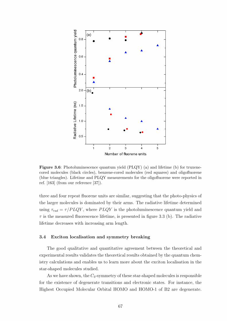
Figure 3.6: Photoluminescence quantum yield (PLQY) (a) and lifetime (b) for truxene-cored molecules (black circles), benzene-cored molecules (red squares) and oligofluorene(blue triangles). Lifetime and PLQY measurements for the oligofluorene were reported inref. [163] (from our reference [37]).

three and four repeat fluorene units are similar, suggesting that the photo-physics of

the larger molecules is dominated by their arms. The radiative lifetime determined

using τrad = τ/PLQY , where PLQY is the photoluminescence quantum yield and

τ is the measured fluorescence lifetime, is presented in figure 3.3 (b). The radiative

lifetime decreases with increasing arm length.

3.4 Exciton localisation and symmetry breaking

The good qualitative and quantitative agreement between the theoretical and

experimental results validates the theoretical results obtained by the quantum chem-

istry calculations and enables us to learn more about the exciton localisation in the

star-shaped molecules studied.

As we have shown, the C3-symmetry of these star-shaped molecules is responsible

for the existence of degenerate transitions and electronic states. For instance, the

Highest Occupied Molecular Orbital HOMO and HOMO-1 of B2 are degenerate.

67

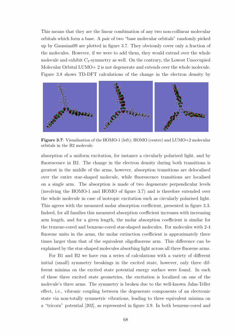
This means that they are the linear combination of any two non-collinear molecular

orbitals which form a base. A pair of two “base molecular orbitals” randomly picked

up by Gaussian09 are plotted in figure 3.7. They obviously cover only a fraction of

the molecules. However, if we were to add them, they would extend over the whole

molecule and exhibit C3-symmetry as well. On the contrary, the Lowest Unoccupied

Molecular Orbital LUMO+ 2 is not degenerate and extends over the whole molecule.

Figure 3.8 shows TD-DFT calculations of the change in the electron density by

Figure 3.7: Visualisation of the HOMO-1 (left); HOMO (centre) and LUMO+2 molecularorbitals in the B2 molecule.

absorption of a uniform excitation, for instance a circularly polarized light, and by

fluorescence in B2. The change in the electron density during both transitions is

greatest in the middle of the arms, however, absorption transitions are delocalised

over the entire star-shaped molecule, while fluorescence transitions are localised

on a single arm. The absorption is made of two degenerate perpendicular levels

(involving the HOMO-1 and HOMO of figure 3.7) and is therefore extended over

the whole molecule in case of isotropic excitation such as circularly polarised light.

This agrees with the measured molar absorption coefficient, presented in figure 3.3.

Indeed, for all families this measured absorption coefficient increases with increasing

arm length, and for a given length, the molar absorption coefficient is similar for

the truxene-cored and benzene-cored star-shaped molecules. For molecules with 2-4

fluorene units in the arms, the molar extinction coefficient is approximately three

times larger than that of the equivalent oligofluorene arm. This difference can be

explained by the star-shaped molecules absorbing light across all three fluorene arms.

For B1 and B2 we have run a series of calculations with a variety of different

initial (small) symmetry breakings in the excited state, however, only three dif-

ferent minima on the excited state potential energy surface were found. In each

of these three excited state geometries, the excitation is localized on one of the

molecule’s three arms. The symmetry is broken due to the well-known Jahn-Teller

effect, i.e., vibronic coupling between the degenerate components of an electronic

state via non-totally symmetric vibrations, leading to three equivalent minima on

a “tricorn” potential [202], as represented in figure 3.9. In both benzene-cored and

68

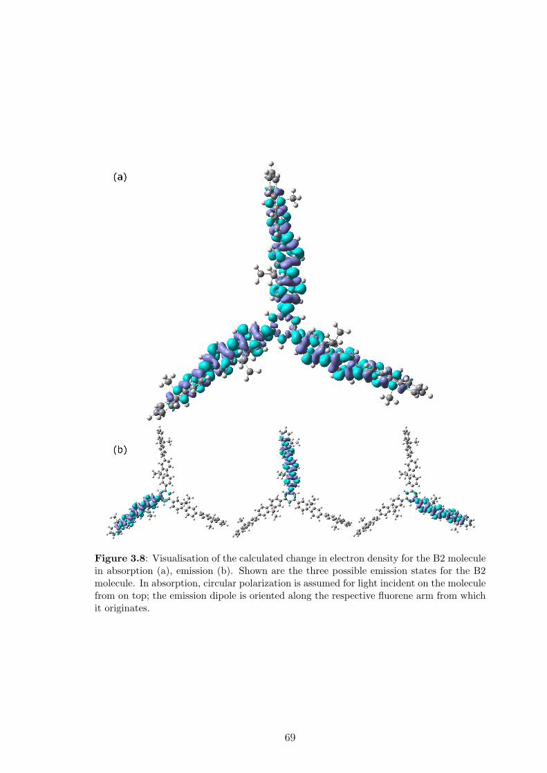
Figure 3.8: Visualisation of the calculated change in electron density for the B2 moleculein absorption (a), emission (b). Shown are the three possible emission states for the B2molecule. In absorption, circular polarization is assumed for light incident on the moleculefrom on top; the emission dipole is oriented along the respective fluorene arm from whichit originates.

69

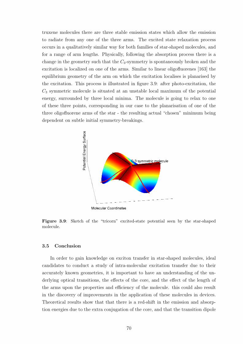
truxene molecules there are three stable emission states which allow the emission

to radiate from any one of the three arms. The excited state relaxation process

occurs in a qualitatively similar way for both families of star-shaped molecules, and

for a range of arm lengths. Physically, following the absorption process there is a

change in the geometry such that the C3-symmetry is spontaneously broken and the

excitation is localized on one of the arms. Similar to linear oligofluorenes [163] the

equilibrium geometry of the arm on which the excitation localises is planarised by

the excitation. This process is illustrated in figure 3.9: after photo-excitation, the

C3 symmetric molecule is situated at an unstable local maximum of the potential

energy, surrounded by three local minima. The molecule is going to relax to one

of these three points, corresponding in our case to the planarisation of one of the

three oligofluorene arms of the star - the resulting actual “chosen” minimum being

dependent on subtle initial symmetry-breakings.

Figure 3.9: Sketch of the “tricorn” excited-state potential seen by the star-shapedmolecule.

3.5 Conclusion

In order to gain knowledge on exciton transfer in star-shaped molecules, ideal

candidates to conduct a study of intra-molecular excitation transfer due to their

accurately known geometries, it is important to have an understanding of the un-

derlying optical transitions, the effects of the core, and the effect of the length of

the arms upon the properties and efficiency of the molecule. this could also result

in the discovery of improvements in the application of these molecules in devices.

Theoretical results show that that there is a red-shift in the emission and absorp-

tion energies due to the extra conjugation of the core, and that the transition dipole

70

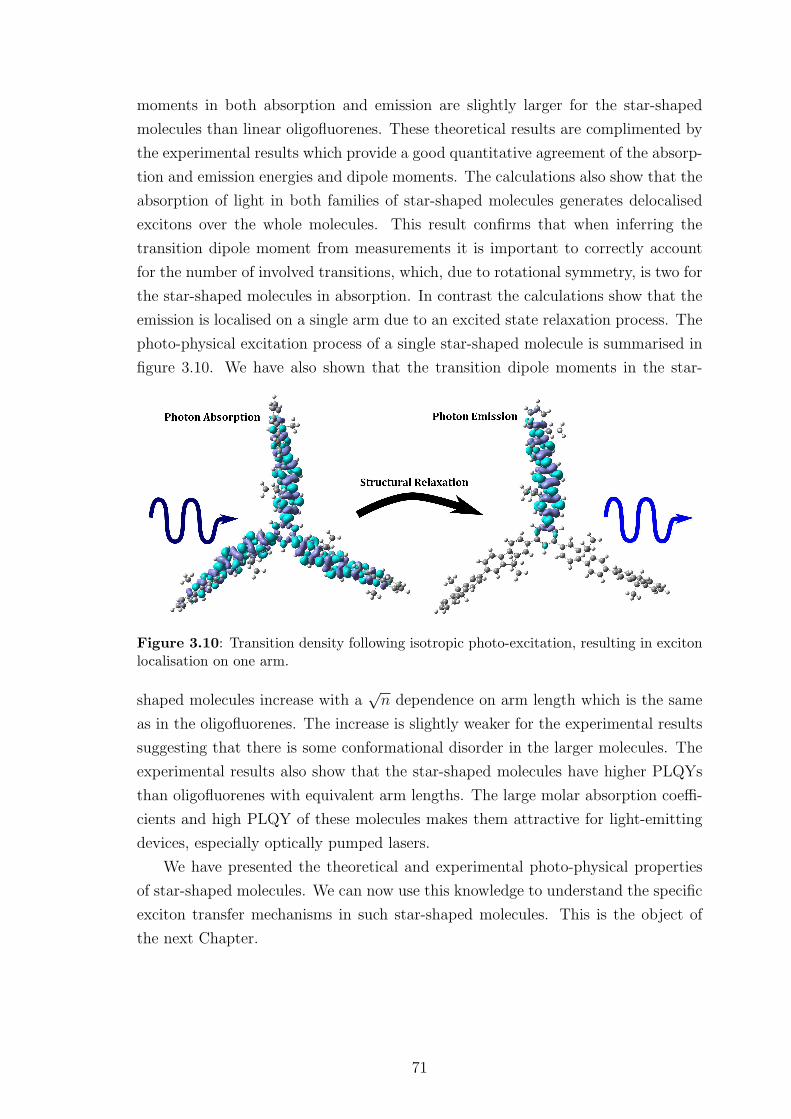
moments in both absorption and emission are slightly larger for the star-shaped

molecules than linear oligofluorenes. These theoretical results are complimented by

the experimental results which provide a good quantitative agreement of the absorp-

tion and emission energies and dipole moments. The calculations also show that the

absorption of light in both families of star-shaped molecules generates delocalised

excitons over the whole molecules. This result confirms that when inferring the

transition dipole moment from measurements it is important to correctly account

for the number of involved transitions, which, due to rotational symmetry, is two for

the star-shaped molecules in absorption. In contrast the calculations show that the

emission is localised on a single arm due to an excited state relaxation process. The

photo-physical excitation process of a single star-shaped molecule is summarised in

figure 3.10. We have also shown that the transition dipole moments in the star-

Figure 3.10: Transition density following isotropic photo-excitation, resulting in excitonlocalisation on one arm.

shaped molecules increase with a√n dependence on arm length which is the same

as in the oligofluorenes. The increase is slightly weaker for the experimental results

suggesting that there is some conformational disorder in the larger molecules. The

experimental results also show that the star-shaped molecules have higher PLQYs

than oligofluorenes with equivalent arm lengths. The large molar absorption coeffi-

cients and high PLQY of these molecules makes them attractive for light-emitting

devices, especially optically pumped lasers.

We have presented the theoretical and experimental photo-physical properties

of star-shaped molecules. We can now use this knowledge to understand the specific

exciton transfer mechanisms in such star-shaped molecules. This is the object of

the next Chapter.

71

Chapter 4

Intra-molecular exciton transfer in C3-symmetric

molecules

Star-shaped molecules are of growing interest as organic optoelectronic materi-

als. In addition, the known geometry of these molecules makes them particularly

useful in understanding intra-molecular exciton transfer. We have gained valuable

knowledge about the optical and electronic properties of some star-shaped molecules,

as seen in the previous Chapter. Based on these results, we report in this Chapter

a detailed theoretical study of the time-resolved photo-physics of the truxene-cored

molecules presented in Chapter 3, combined with experiments through the use of

fluorescence depolarisation. This combined experimental and theoretical study en-

ables us to gain valuable knowledge about the mechanisms responsible for exciton

migration in solutions of these star-shaped molecules.

4.1 Background

We have shown in Chapter 3 that star-shaped molecules are of research inter-

est due to their ease of experimental processing. In addition, branched conjugated

molecules in general show attractive properties such as directional energy trans-

fer [203], enhanced two photon absorption [204–206], and high photoluminescence

quantum yield in the solid state [81, 207]. These properties make them useful in

light harvesting systems for solar energy conversion [203,208,209], fluorescence sen-

sors [210,211], organic light emitting diodes [183,212] and organic lasers [81,82]. In

order to design efficient light-harvesting antennae which would absorb light and fun-

nel energy to a desired location, it is important to understand exciton localisation

and energy transfer.

A number of experimental and theoretical studies investigating exciton locali-

sation have been carried out on branched molecules with different chemical struc-

tures, observing their fluorescence [213, 214] or transient absorption [215]. The de-

polarisation of fluorescence also provides complementary information about energy

transfer, as it shows the change in orientation of the emission dipole from the ab-

sorption dipole. Molecules with a nitrogen core [65,213–216] show a very fast energy

transfer between branches on a 30 fs time scale and subsequent localisation on one

branch [215]. In contrast the molecules with benzene [217–219], carbon and adaman-

tine cores show much slower depolarisation which implies that excitation localises

72

quickly on one branch [218] and subsequently transfers to other branches via Forster

hopping [219].

For the truxene- and benzene-cored star-shaped molecules presented in Chapter

3, there has been a small amount of work carried out on their fluorescence dynamics,

in a study of the picosecond planarisation process of the branches [220]. However,

there has yet to be a study of energy transfer and exciton localisation in truxene-

and benzene-cored molecules. This work is the subject of this Chapter. We believe

that, regarding the photo-physics results presented in Chapter 3, the benzene- and

truxene-cored star-shaped molecules behave in a qualitatively similar fashion, and

we thus restrict our study to truxene-cored molecules.

4.2 Fluorescence anisotropy theory

4.2.1 Background to fluorescence anisotropy

The fluorescence anisotropy technique provides an experimentally accessible

measure of the relative orientation of the fluorescence dipole compared to the absorp-

tion dipole. The principle lies in the excitation of a sample by a linearly polarised

pulse, and by then recording separately the intensities emitted by the excited sam-

ple in the directions parallel and perpendicular to the linearly polarised excitation

pulse. It is thus possible to monitor the average transition dipole angle and rotation

(due to, for instance, molecular relaxation, Forster transfer or molecular movement),

with respect to the excitation pulse [221].

The quantitative measure of the fluorescence anisotropy, usually denoted as r,

is given by the following formula [221]:

r =I‖ − I⊥I‖ + 2I⊥

, (4.1)

where I‖ and I⊥ are the fluorescence intensities respectively parallel and perpendicu-

lar to the linearly polarised pump. Polarisation-independent fluorescence dynamics,

the intensity recorded at the “magic angle” m, is, in our work, reconstructed from

the parallel and perpendicular intensities using:

m =I‖ + 2I⊥

3. (4.2)

In the rest of this thesis, “magic angle” will be used to refer to this quantity, which

is the polarisation-independent fluorescence intensity.

73

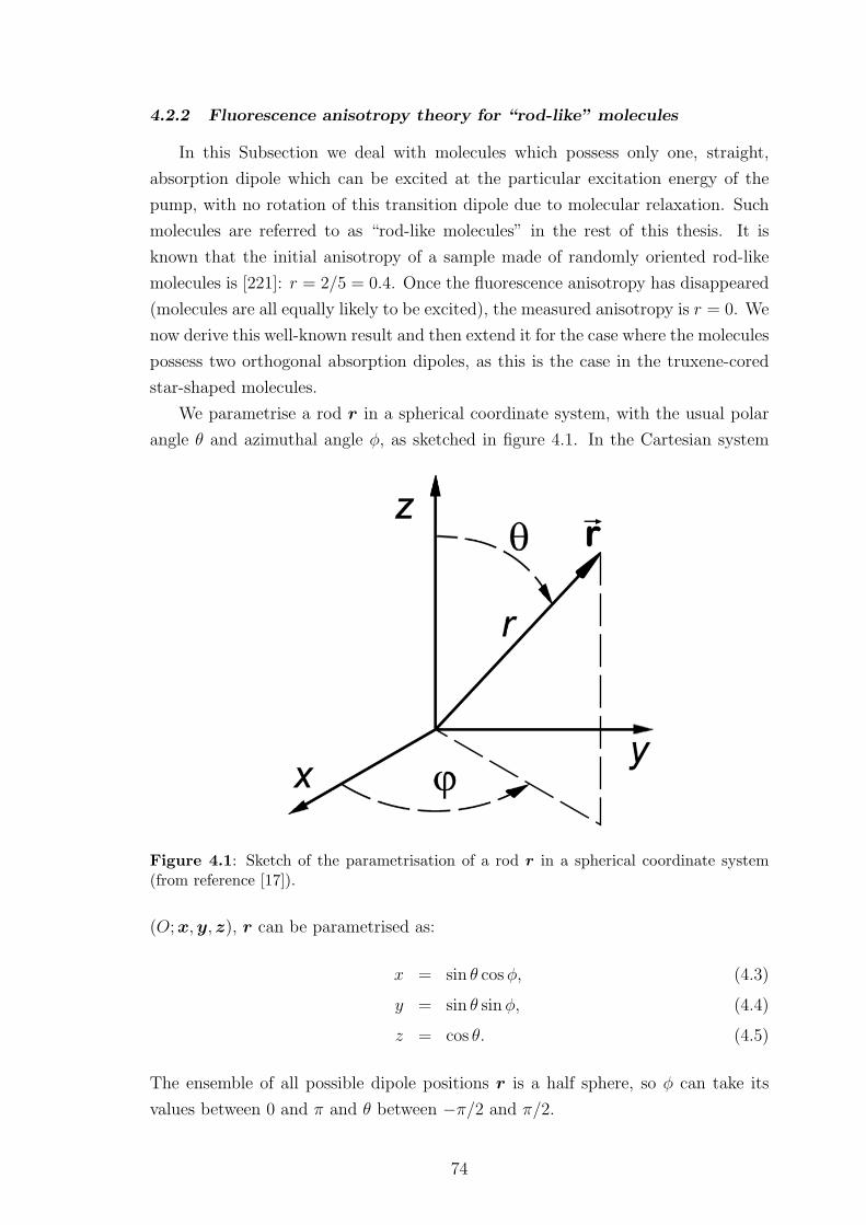
4.2.2 Fluorescence anisotropy theory for “rod-like” molecules

In this Subsection we deal with molecules which possess only one, straight,

absorption dipole which can be excited at the particular excitation energy of the

pump, with no rotation of this transition dipole due to molecular relaxation. Such

molecules are referred to as “rod-like molecules” in the rest of this thesis. It is

known that the initial anisotropy of a sample made of randomly oriented rod-like

molecules is [221]: r = 2/5 = 0.4. Once the fluorescence anisotropy has disappeared

(molecules are all equally likely to be excited), the measured anisotropy is r = 0. We

now derive this well-known result and then extend it for the case where the molecules

possess two orthogonal absorption dipoles, as this is the case in the truxene-cored

star-shaped molecules.

We parametrise a rod r in a spherical coordinate system, with the usual polar

angle θ and azimuthal angle φ, as sketched in figure 4.1. In the Cartesian system

Figure 4.1: Sketch of the parametrisation of a rod r in a spherical coordinate system(from reference [17]).

(O;x,y, z), r can be parametrised as:

x = sin θ cosφ, (4.3)

y = sin θ sinφ, (4.4)

z = cos θ. (4.5)

The ensemble of all possible dipole positions r is a half sphere, so φ can take its

values between 0 and π and θ between −π/2 and π/2.

74

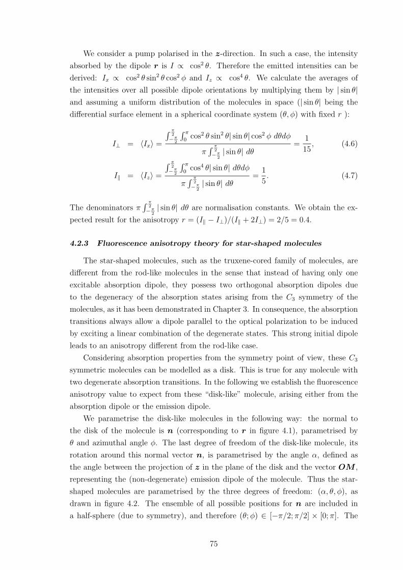
We consider a pump polarised in the z-direction. In such a case, the intensity

absorbed by the dipole r is I ∝ cos2 θ. Therefore the emitted intensities can be

derived: Ix ∝ cos2 θ sin2 θ cos2 φ and Iz ∝ cos4 θ. We calculate the averages of

the intensities over all possible dipole orientations by multiplying them by | sin θ|and assuming a uniform distribution of the molecules in space (| sin θ| being the

differential surface element in a spherical coordinate system (θ, φ) with fixed r ):

I⊥ = 〈Ix〉 =∫ π

2

−π2

∫ π

0cos2 θ sin2 θ| sin θ| cos2 φ dθdφ

π∫ π

2

−π2

| sin θ| dθ=

1

15, (4.6)

I‖ = 〈Iz〉 =∫ π

2

−π2

∫ π

0cos4 θ| sin θ| dθdφ

π∫ π

2

−π2

| sin θ| dθ=

1

5. (4.7)

The denominators π∫ π

2

−π2

| sin θ| dθ are normalisation constants. We obtain the ex-

pected result for the anisotropy r = (I‖ − I⊥)/(I‖ + 2I⊥) = 2/5 = 0.4.

4.2.3 Fluorescence anisotropy theory for star-shaped molecules

The star-shaped molecules, such as the truxene-cored family of molecules, are

different from the rod-like molecules in the sense that instead of having only one

excitable absorption dipole, they possess two orthogonal absorption dipoles due

to the degeneracy of the absorption states arising from the C3 symmetry of the

molecules, as it has been demonstrated in Chapter 3. In consequence, the absorption

transitions always allow a dipole parallel to the optical polarization to be induced

by exciting a linear combination of the degenerate states. This strong initial dipole

leads to an anisotropy different from the rod-like case.

Considering absorption properties from the symmetry point of view, these C3

symmetric molecules can be modelled as a disk. This is true for any molecule with

two degenerate absorption transitions. In the following we establish the fluorescence

anisotropy value to expect from these “disk-like” molecule, arising either from the

absorption dipole or the emission dipole.

We parametrise the disk-like molecules in the following way: the normal to

the disk of the molecule is n (corresponding to r in figure 4.1), parametrised by

θ and azimuthal angle φ. The last degree of freedom of the disk-like molecule, its

rotation around this normal vector n, is parametrised by the angle α, defined as

the angle between the projection of z in the plane of the disk and the vector OM ,

representing the (non-degenerate) emission dipole of the molecule. Thus the star-

shaped molecules are parametrised by the three degrees of freedom: (α, θ, φ), as

drawn in figure 4.2. The ensemble of all possible positions for n are included in

a half-sphere (due to symmetry), and therefore (θ;φ) ∈ [−π/2; π/2] × [0; π]. The

75

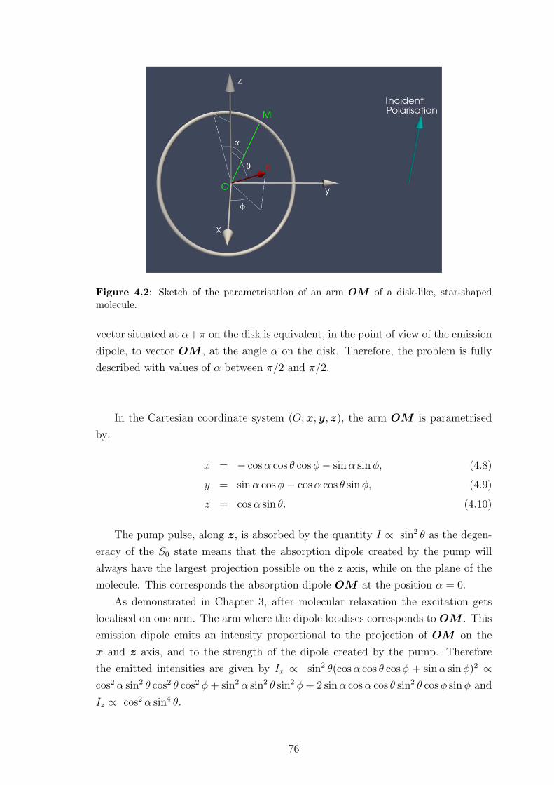
Figure 4.2: Sketch of the parametrisation of an arm OM of a disk-like, star-shapedmolecule.

vector situated at α+π on the disk is equivalent, in the point of view of the emission

dipole, to vector OM , at the angle α on the disk. Therefore, the problem is fully

described with values of α between π/2 and π/2.

In the Cartesian coordinate system (O;x,y, z), the arm OM is parametrised

by:

x = − cosα cos θ cosφ− sinα sinφ, (4.8)

y = sinα cosφ− cosα cos θ sinφ, (4.9)

z = cosα sin θ. (4.10)

The pump pulse, along z, is absorbed by the quantity I ∝ sin2 θ as the degen-

eracy of the S0 state means that the absorption dipole created by the pump will

always have the largest projection possible on the z axis, while on the plane of the

molecule. This corresponds the absorption dipole OM at the position α = 0.

As demonstrated in Chapter 3, after molecular relaxation the excitation gets

localised on one arm. The arm where the dipole localises corresponds to OM . This

emission dipole emits an intensity proportional to the projection of OM on the

x and z axis, and to the strength of the dipole created by the pump. Therefore

the emitted intensities are given by Ix ∝ sin2 θ(cosα cos θ cosφ + sinα sinφ)2 ∝cos2 α sin2 θ cos2 θ cos2 φ + sin2 α sin2 θ sin2 φ + 2 sinα cosα cos θ sin2 θ cosφ sinφ and

Iz ∝ cos2 α sin4 θ.

76

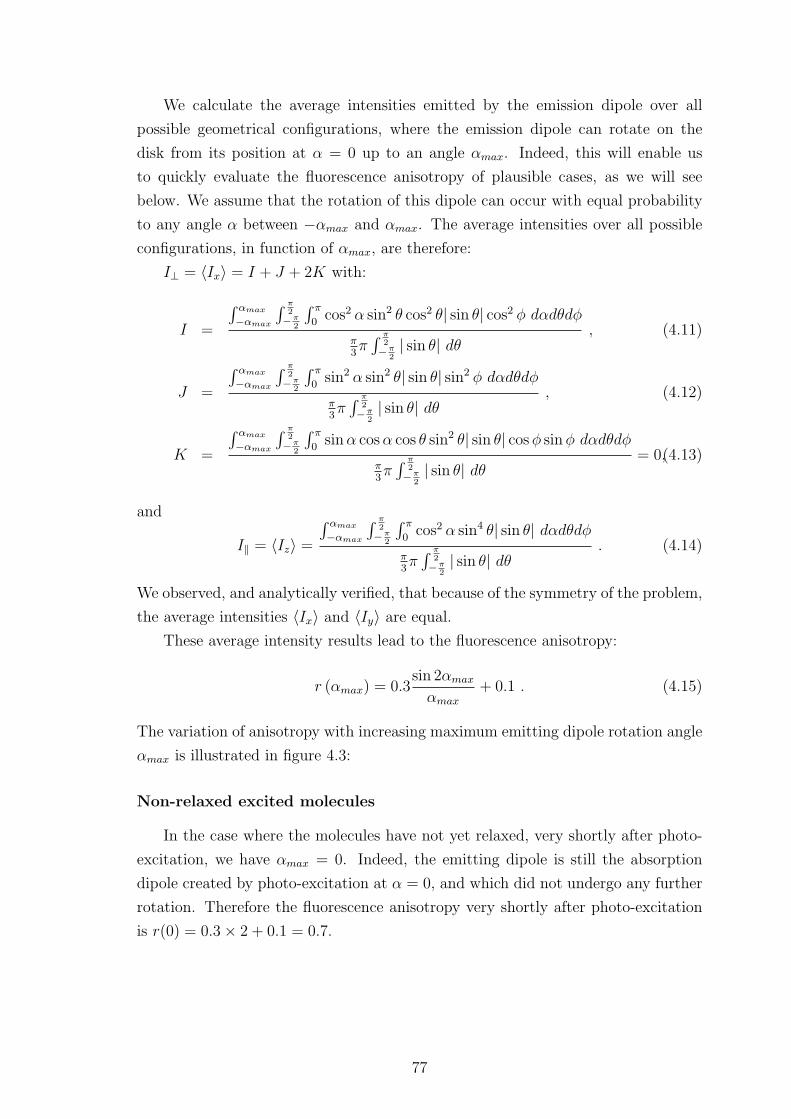
We calculate the average intensities emitted by the emission dipole over all

possible geometrical configurations, where the emission dipole can rotate on the

disk from its position at α = 0 up to an angle αmax. Indeed, this will enable us

to quickly evaluate the fluorescence anisotropy of plausible cases, as we will see

below. We assume that the rotation of this dipole can occur with equal probability

to any angle α between −αmax and αmax. The average intensities over all possible

configurations, in function of αmax, are therefore:

I⊥ = 〈Ix〉 = I + J + 2K with:

I =

∫ αmax

−αmax

∫ π2

−π2

∫ π

0cos2 α sin2 θ cos2 θ| sin θ| cos2 φ dαdθdφ

π3π∫ π

2

−π2

| sin θ| dθ, (4.11)

J =

∫ αmax

−αmax

∫ π2

−π2

∫ π

0sin2 α sin2 θ| sin θ| sin2 φ dαdθdφ

π3π∫ π

2

−π2

| sin θ| dθ, (4.12)

K =

∫ αmax

−αmax

∫ π2

−π2

∫ π

0sinα cosα cos θ sin2 θ| sin θ| cosφ sinφ dαdθdφ

π3π∫ π

2

−π2

| sin θ| dθ= 0,(4.13)

and

I‖ = 〈Iz〉 =∫ αmax

−αmax

∫ π2

−π2

∫ π

0cos2 α sin4 θ| sin θ| dαdθdφ

π3π∫ π

2

−π2

| sin θ| dθ. (4.14)

We observed, and analytically verified, that because of the symmetry of the problem,

the average intensities 〈Ix〉 and 〈Iy〉 are equal.

These average intensity results lead to the fluorescence anisotropy:

r (αmax) = 0.3sin 2αmax

αmax

+ 0.1 . (4.15)

The variation of anisotropy with increasing maximum emitting dipole rotation angle

αmax is illustrated in figure 4.3:

Non-relaxed excited molecules

In the case where the molecules have not yet relaxed, very shortly after photo-

excitation, we have αmax = 0. Indeed, the emitting dipole is still the absorption

dipole created by photo-excitation at α = 0, and which did not undergo any further

rotation. Therefore the fluorescence anisotropy very shortly after photo-excitation

is r(0) = 0.3× 2 + 0.1 = 0.7.

77

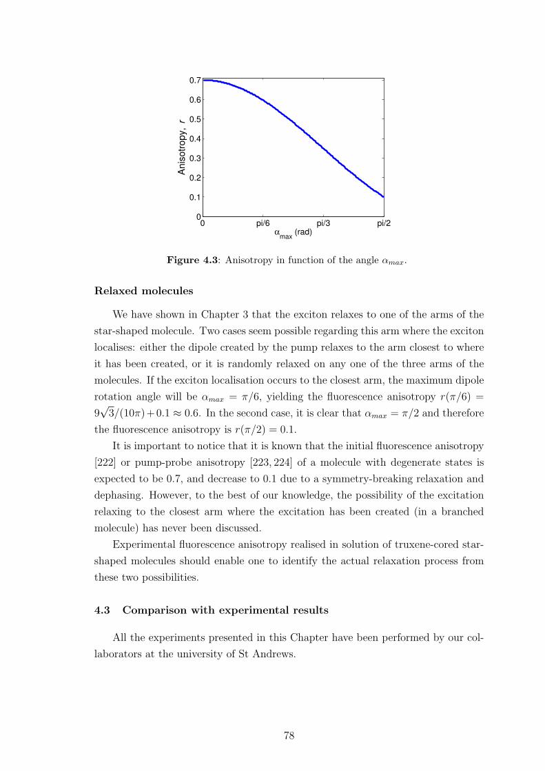
0 pi/6 pi/3 pi/20

0.1

0.2

0.3

0.4

0.5

0.6

0.7

Anis

otr

opy,

r

αmax

(rad)

Figure 4.3: Anisotropy in function of the angle αmax.

Relaxed molecules

We have shown in Chapter 3 that the exciton relaxes to one of the arms of the

star-shaped molecule. Two cases seem possible regarding this arm where the exciton

localises: either the dipole created by the pump relaxes to the arm closest to where

it has been created, or it is randomly relaxed on any one of the three arms of the

molecules. If the exciton localisation occurs to the closest arm, the maximum dipole

rotation angle will be αmax = π/6, yielding the fluorescence anisotropy r(π/6) =

9√3/(10π)+0.1 ≈ 0.6. In the second case, it is clear that αmax = π/2 and therefore

the fluorescence anisotropy is r(π/2) = 0.1.

It is important to notice that it is known that the initial fluorescence anisotropy

[222] or pump-probe anisotropy [223, 224] of a molecule with degenerate states is

expected to be 0.7, and decrease to 0.1 due to a symmetry-breaking relaxation and

dephasing. However, to the best of our knowledge, the possibility of the excitation

relaxing to the closest arm where the excitation has been created (in a branched

molecule) has never been discussed.

Experimental fluorescence anisotropy realised in solution of truxene-cored star-

shaped molecules should enable one to identify the actual relaxation process from

these two possibilities.

4.3 Comparison with experimental results

All the experiments presented in this Chapter have been performed by our col-

laborators at the university of St Andrews.

78

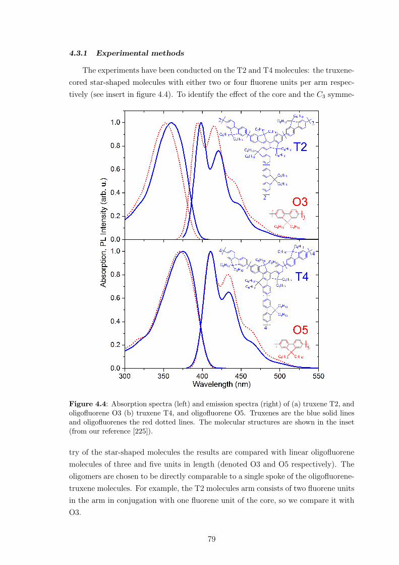
4.3.1 Experimental methods

The experiments have been conducted on the T2 and T4 molecules: the truxene-

cored star-shaped molecules with either two or four fluorene units per arm respec-

tively (see insert in figure 4.4). To identify the effect of the core and the C3 symme-

Figure 4.4: Absorption spectra (left) and emission spectra (right) of (a) truxene T2, andoligofluorene O3 (b) truxene T4, and oligofluorene O5. Truxenes are the blue solid linesand oligofluorenes the red dotted lines. The molecular structures are shown in the inset(from our reference [225]).

try of the star-shaped molecules the results are compared with linear oligofluorene

molecules of three and five units in length (denoted O3 and O5 respectively). The

oligomers are chosen to be directly comparable to a single spoke of the oligofluorene-

truxene molecules. For example, the T2 molecules arm consists of two fluorene units

in the arm in conjugation with one fluorene unit of the core, so we compare it with

O3.

79

Ultra-fast photoluminescence dynamics were measured using fluorescence spec-

troscopy. The emitted intensities are filtered by a narrow bandwidth filter (less

than 5 nm wide), centred around a given detection wavelength. The pump source

has pulses of full-width half-maximum (FWHM) 100 fs. The photolumiscence (PL)

is recorded in the direction perpendicular and parallel to the excitation to derive

the fluorescence anisotropy. The temporal shifts in recorded PL between parallel

and perpendicular excitation were obtained by recording the water Raman signal

for both polarisations and finding the shift between the two. The shifts were 39 fs

at 380 nm, 32 fs at 400 nm and 38 fs at 420 nm excitation: all anisotropy data were

corrected for this temporal shift before fitting.

Fitting was carried out using the impulse reconvolution method [226]. This

involves firstly fitting a convolved function to the reconstructed magic angle data

I‖ + 2I⊥, denoted as the sum fit. The fitting parameters are then multiplied by the

trial function for the anisotropy decay and convolved with the instrument response

function (IRF). This function is compared with the numerator of the anisotropy

equation I‖ − I⊥, the so-called difference fit. A full description of fitting is given in

reference [225].

It was checked that the kinetics and anisotropy decays were concentration in-

dependent, in the low-concentration range used, when detecting the fluorescence at

the 0-1 vibronic peak and longer wavelengths.

The excitation wavelength λex was chosen such that it is as close to the peak

of the absorption as the experimental setup would allow, whilst the detection wave-

length λdet was chosen to be on the red side of the 0-1 peak to remove any effects of

self-absorption on the recorded dynamics. It was found that the observed anisotropy

decay was independent of detection wavelength, a result that has previously been

noted in reference [227].

4.3.2 Experimental results

Figure 4.4 shows experimental absorption and time integrated fluorescence spec-

tra of the branched molecules T2 and T4 and of the linear molecules O3 and O5.

The upper panels of figure 4.5 show the reconstructed fluorescence kinetics at the

magic angle for all of the studied molecules, with λex = 380 nm and λdet = 420 nm

(O3 and T2) and λex = 380 nm and λdet = 440 nm (O5 and T4). The lower panels

show the corresponding anisotropy decays calculated using equation (4.2).

Magic angle kinetics for both branched and linear molecules show a finite rise of

∼ 90 fs which is more clearly visible when compared against an instantaneous rise

with a magnified scale shown in the insets. Both branched and linear molecules show

an initial anisotropy of 0.4 but only the branched molecules show fast depolarisation

on a sub-picosecond time scale. The T2 anisotropy shows a fast initial decay from 0.4

80

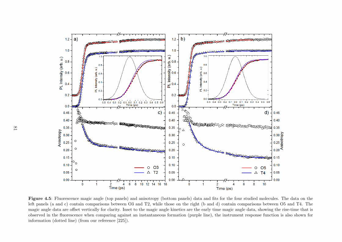
Figure 4.5: Fluorescence magic angle (top panels) and anisotropy (bottom panels) data and fits for the four studied molecules. The data on theleft panels (a and c) contain comparisons between O3 and T2, while those on the right (b and d) contain comparisons between O5 and T4. Themagic angle data are offset vertically for clarity. Inset to the magic angle kinetics are the early time magic angle data, showing the rise-time that isobserved in the fluorescence when comparing against an instantaneous formation (purple line), the instrument response function is also shown forinformation (dotted line) (from our reference [225]).

81

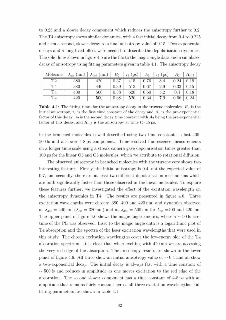
to 0.25 and a slower decay component which reduces the anisotropy further to 0.2.

The T4 anisotropy shows similar dynamics, with a fast initial decay from 0.4 to 0.225

and then a second, slower decay to a final anisotropy value of 0.15. Two exponential

decays and a long-lived offset were needed to describe the depolarisation dynamics.

The solid lines shown in figure 4.5 are the fits to the magic angle data and a simulated

decay of anisotropy using fitting parameters given in table 4.1. The anisotropy decay

Molecule λex (nm) λdet (nm) R0 τ1 (ps) A1 τ2 (ps) A2 Rinf

T2 380 420 0.37 415 0.76 8.4 0.24 0.19T4 380 440 0.39 513 0.67 2.9 0.33 0.15T4 400 500 0.38 520 0.60 5.2 0.4 0.18T4 420 500 0.38 520 0.34 7.9 0.66 0.24

Table 4.1: The fitting times for the anisotropy decay in the truxene molecules. R0 is theinitial anisotropy, τ1 is the first time constant of the decay and A1 is the pre-exponentialfactor of this decay. τ2 is the second decay time constant with A2 being the pre-exponentialfactor of this decay, and Rinf is the anisotropy at time t> 15 ps.

in the branched molecules is well described using two time constants, a fast 400-

500 fs and a slower 4-8 ps component. Time-resolved fluorescence measurements

on a longer time scale using a streak camera gave depolarisation times greater than

100 ps for the linear O3 and O5 molecules, which we attribute to rotational diffusion.

The observed anisotropy in branched molecules with the truxene core shows two

interesting features. Firstly, the initial anisotropy is 0.4, not the expected value of

0.7, and secondly, there are at least two different depolarisation mechanisms which

are both significantly faster than those observed in the linear molecules. To explore

these features further, we investigated the effect of the excitation wavelength on

the anisotropy dynamics in T4. The results are presented in figure 4.6. Three

excitation wavelengths were chosen: 380, 400 and 420 nm, and dynamics observed

at λdet = 440 nm (λex = 380 nm) and at λdet = 500 nm for λex =400 and 420 nm.

The upper panel of figure 4.6 shows the magic angle kinetics, where a ∼ 90 fs rise-

time of the PL was observed. Inset to the magic angle data is a logarithmic plot of

T4 absorption and the spectra of the laser excitation wavelengths that were used in

this study. The chosen excitation wavelengths cover the low-energy side of the T4

absorption spectrum. It is clear that when exciting with 420 nm we are accessing

the very red edge of the absorption. The anisotropy results are shown in the lower

panel of figure 4.6. All three show an initial anisotropy value of ∼ 0.4 and all show

a two-exponential decay. The initial decay is always fast with a time constant of

∼ 500 fs and reduces in amplitude as one moves excitation to the red edge of the

absorption. The second slower component has a time constant of 4-8 ps with an

amplitude that remains fairly constant across all three excitation wavelengths. Full

fitting parameters are shown in table 4.1.

82

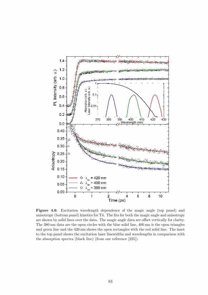
Figure 4.6: Excitation wavelength dependence of the magic angle (top panel) andanisotropy (bottom panel) kinetics for T4. The fits for both the magic angle and anisotropyare shown by solid lines over the data. The magic angle data are offset vertically for clarity.The 380 nm data are the open circles with the blue solid line, 400 nm is the open trianglesand green line and the 420 nm shows the open rectangles with the red solid line. The insetto the top panel shows the excitation laser linewidths and wavelengths in comparison withthe absorption spectra (black line) (from our reference [225]).

83

The observed anisotropy values differ greatly from the values we predicted in

Section 4.2.3. Indeed, assuming perfect symmetry of the star-shaped molecules and

therefore degenerate absorption energies, we had calculated that the initial value

of the anisotropy should be 0.7, and that it should then decay to either 0.6 or

0.1 due to the molecular relaxations. These final anisotropy values depend on two

possible scenarios: either the excitation is transferred to the arm closest to where

the excitation was created (r = 0.6), or to a random arm (r = 0.1). However, none

of these predicted values are observed experimentally. We will examine possible

explanations to explain this discrepancy, until one of these explanations fully resist

the comparison with experiments. This is the purpose of the rest of this Chapter.

4.4 Proposed theory I: two-step exciton transfer in “disk-like” molecules

The presented anisotropy measurements are detected in the emission wavelength

range of the molecules, therefore they correspond to a molecule in its relaxed excited

state. A value of the anisotropy between 0.1 and 0.6 is thus expected. We observe

experimental values between these two values, and a fast decay. In this Section we

present theoretical results in order to verify if the discrepancy between the fluo-

rescence anisotropy results we observed and the results we expected for “disk-like”

molecules is coming from rotation of the transition dipole from the arm closest to

where it was created to any of the other arms, and from experimental artefacts. In-

deed, the IRF, pulse length, and the anisotropy decay have comparable time-scales,

so we must carefully account for the inter-mixing convolution of these effects, which

could lead to measured results different from expected.

4.4.1 Method

We assume that the star-shape molecules behave like the “disk-like” molecules of

Section 4.2.3. As the anisotropy is detected around the emission energy, we assume

that all the star-shaped molecules have relaxed to their excited-state geometries

when the anisotropy is detected. It follows that the excitation is relaxed to an

actual arm of the molecule, as we have seen in Chapter 3. We make the assumption

that this arm is the closest to where the excitation has been created (otherwise

the fluorescence anisotropy would stay constant at r = 0.1). We believe that the

excitation can transfer to one of the other two arms from there (otherwise no decay

of anisotropy would be observed). These assumptions being established, we can

build a model to formalise them and take into account the effects of the pump pulse

width and the experimental IRF. We have therefore constructed a set of equations

to model the early time-dynamics of excitations:

84

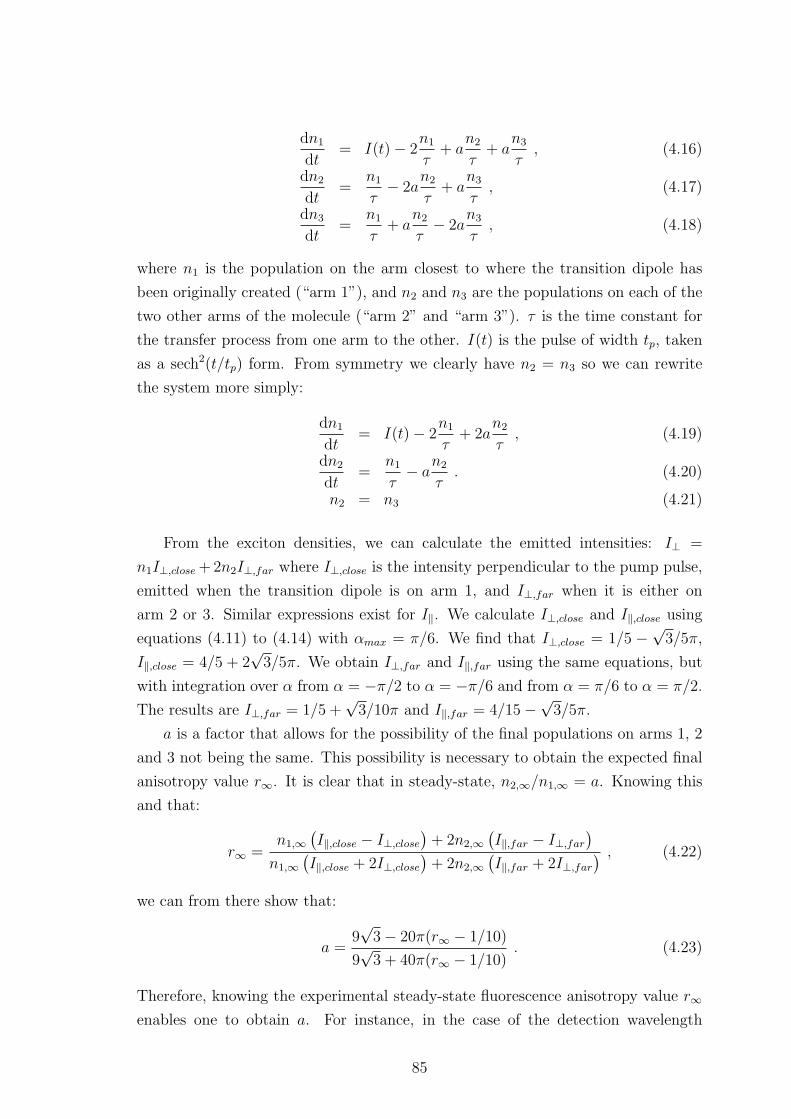
dn1

dt= I(t)− 2

n1

τ+ a

n2

τ+ a

n3

τ, (4.16)

dn2

dt=

n1

τ− 2a

n2

τ+ a

n3

τ, (4.17)

dn3

dt=

n1

τ+ a

n2

τ− 2a

n3

τ, (4.18)

where n1 is the population on the arm closest to where the transition dipole has

been originally created (“arm 1”), and n2 and n3 are the populations on each of the

two other arms of the molecule (“arm 2” and “arm 3”). τ is the time constant for

the transfer process from one arm to the other. I(t) is the pulse of width tp, taken

as a sech2(t/tp) form. From symmetry we clearly have n2 = n3 so we can rewrite

the system more simply:

dn1

dt= I(t)− 2

n1

τ+ 2a

n2

τ, (4.19)

dn2

dt=

n1

τ− a

n2

τ. (4.20)

n2 = n3 (4.21)

From the exciton densities, we can calculate the emitted intensities: I⊥ =

n1I⊥,close+2n2I⊥,far where I⊥,close is the intensity perpendicular to the pump pulse,

emitted when the transition dipole is on arm 1, and I⊥,far when it is either on

arm 2 or 3. Similar expressions exist for I‖. We calculate I⊥,close and I‖,close using

equations (4.11) to (4.14) with αmax = π/6. We find that I⊥,close = 1/5 −√3/5π,

I‖,close = 4/5 + 2√3/5π. We obtain I⊥,far and I‖,far using the same equations, but

with integration over α from α = −π/2 to α = −π/6 and from α = π/6 to α = π/2.

The results are I⊥,far = 1/5 +√3/10π and I‖,far = 4/15−

√3/5π.

a is a factor that allows for the possibility of the final populations on arms 1, 2

and 3 not being the same. This possibility is necessary to obtain the expected final

anisotropy value r∞. It is clear that in steady-state, n2,∞/n1,∞ = a. Knowing this

and that:

r∞ =n1,∞

(I‖,close − I⊥,close

)+ 2n2,∞

(I‖,far − I⊥,far

)

n1,∞

(I‖,close + 2I⊥,close

)+ 2n2,∞

(I‖,far + 2I⊥,far

) , (4.22)

we can from there show that:

a =9√3− 20π(r∞ − 1/10)

9√3 + 40π(r∞ − 1/10)

. (4.23)

Therefore, knowing the experimental steady-state fluorescence anisotropy value r∞

enables one to obtain a. For instance, in the case of the detection wavelength

85

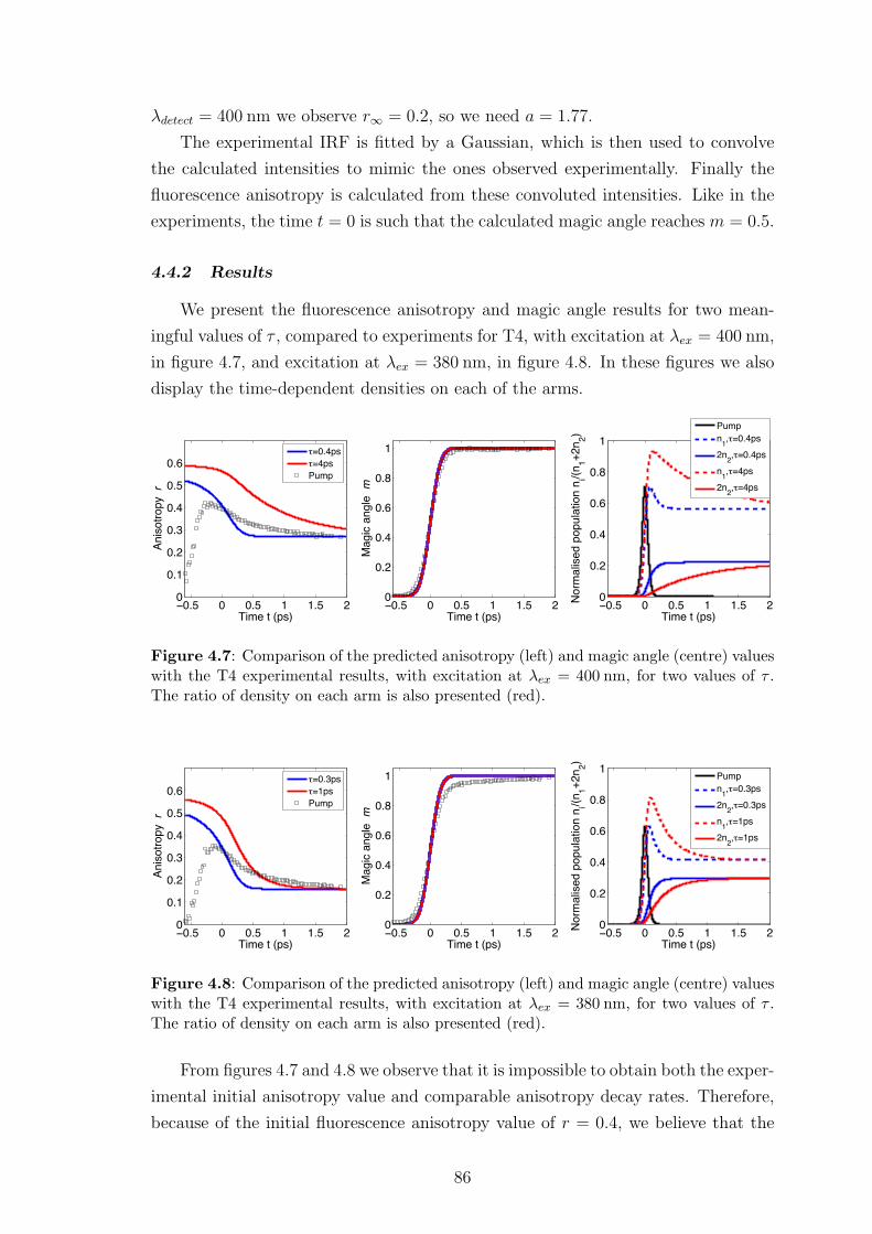
λdetect = 400 nm we observe r∞ = 0.2, so we need a = 1.77.

The experimental IRF is fitted by a Gaussian, which is then used to convolve

the calculated intensities to mimic the ones observed experimentally. Finally the

fluorescence anisotropy is calculated from these convoluted intensities. Like in the

experiments, the time t = 0 is such that the calculated magic angle reaches m = 0.5.

4.4.2 Results

We present the fluorescence anisotropy and magic angle results for two mean-

ingful values of τ , compared to experiments for T4, with excitation at λex = 400 nm,

in figure 4.7, and excitation at λex = 380 nm, in figure 4.8. In these figures we also

display the time-dependent densities on each of the arms.

0.5 0 0.5 1 1.5 20

0.1

0.2

0.3

0.4

0.5

0.6

Time t (ps)

Anis

otr

opy r

=0.4ps

=4ps

Pump

0.5 0 0.5 1 1.5 20

0.2

0.4

0.6

0.8

1

Time t (ps)

Magic

angle

m

0.5 0 0.5 1 1.5 20

0.2

0.4

0.6

0.8

1

Time t (ps)

Norm

alis

ed p

opula

tion n

i/(n

1+

2n

2)

Pump

n1, =0.4ps

2n2, =0.4ps

n1, =4ps

2n2, =4ps

Figure 4.7: Comparison of the predicted anisotropy (left) and magic angle (centre) valueswith the T4 experimental results, with excitation at λex = 400 nm, for two values of τ .The ratio of density on each arm is also presented (red).

0.5 0 0.5 1 1.5 20

0.1

0.2

0.3

0.4

0.5

0.6

Time t (ps)

Anis

otr

opy r

=0.3ps

=1ps

Pump

0.5 0 0.5 1 1.5 20

0.2

0.4

0.6

0.8

1

Time t (ps)

Magic

angle

m

0.5 0 0.5 1 1.5 20

0.2

0.4

0.6

0.8

1

Time t (ps)

Norm

alis

ed p

opula

tion n

i/(n

1+

2n

2)

Pump

n1, =0.3ps

2n2, =0.3ps

n1, =1ps

2n2, =1ps

Figure 4.8: Comparison of the predicted anisotropy (left) and magic angle (centre) valueswith the T4 experimental results, with excitation at λex = 380 nm, for two values of τ .The ratio of density on each arm is also presented (red).

From figures 4.7 and 4.8 we observe that it is impossible to obtain both the exper-

imental initial anisotropy value and comparable anisotropy decay rates. Therefore,

because of the initial fluorescence anisotropy value of r = 0.4, we believe that the

86

star-shaped molecule could behave like a rod-like molecule. That would mean that,

as a consequence of a slight geometrical symmetry-breaking defect, the molecules

are “not C3-symmetric enough” for the degeneracy of the absorption level to exist.

An existing explanation for such low fluorescence anisotropy values is that in fluores-

cence the molecule has already undergone a fast relaxation into a localised emitting

state [215]. Others have also discussed issues of polarity of solvents breaking the

symmetry of the molecules so that the degeneracy is lifted [227] (it is important

to note that the solvent used experimentally here is non-polar). This possibility of

the existence of symmetry-broken star-shaped molecules as a way to explain a lower

value of the measured fluorescence anisotropy is discussed in the next Section.

4.5 Proposed theory II: influence of symmetry-breaking defects

4.5.1 Method

To explore the degree by which the symmetry of the molecule might be broken

by thermally excited conformers, thereby inducing a splitting of the degenerate

lowest transition, we have conducted a series of quantum chemistry calculations on

the truxene molecule for a variety of conformational distortions. If we can find

distortions which produce a sufficiently large splitting at an energy cost of less than

kBT then in our room temperature experiments different ensembles of conformers

will be excited at different wavelengths. Hence their subsequent relaxation pathways

may be different. These calculations were performed on T2 and T4 molecules for

non-symmetric conformations. We started with the C3-symmetric S0 geometries

described in Chapter 3. Some other stable configurations corresponding to local

minima also exist, for example, where some fluorene units of one arm are flipped

over by 180. The energy of these configurations is not much higher than the C3-

symmetric case (typically, 5 meV higher) but the energy barrier is estimated to be

more than 45 meV. The resulting energy splitting is quite small, less than 1 nm,

because the π-conjugation between the fluorene units does not change much by a

180 twist. Here we are interested in out-of-equilibrium configurations, showing

that thermal energy can easily create, from these local minima, some symmetry-

breaking defects having a non-negligible effect on the degeneracy of the absorption

states. In the rest of the quantum chemistry calculations presented in this chapter,

we use the global minima as the equilibrium position, but the reasoning is valid

from the other local minima as well. This optimised equilibrium geometry was

then slightly distorted by us in a variety of ways as described below to create a

“defect” breaking the perfect three-fold rotational symmetry. After this defect is

introduced no further geometry optimisation is performed, as this “defect” is treated

as an out-of-equilibrium configuration. Therefore, to estimate the formation cost of

87

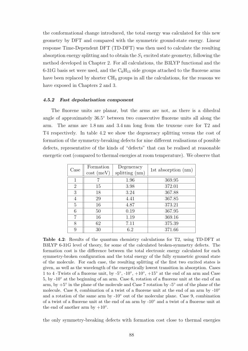
the conformational change introduced, the total energy was calculated for this new

geometry by DFT and compared with the symmetric ground-state energy. Linear

response Time-Dependent DFT (TD-DFT) was then used to calculate the resulting

absorption energy splitting and to obtain the S1 excited state geometry, following the

method developed in Chapter 2. For all calculations, the B3LYP functional and the

6-31G basis set were used, and the C6H13 side groups attached to the fluorene arms

have been replaced by shorter CH3 groups in all the calculations, for the reasons we

have exposed in Chapters 2 and 3.

4.5.2 Fast depolarisation component

The fluorene units are planar, but the arms are not, as there is a dihedral

angle of approximately 36.5 between two consecutive fluorene units all along the

arm. The arms are 1.8 nm and 3.4 nm long from the truxene core for T2 and

T4 respectively. In table 4.2 we show the degeneracy splitting versus the cost of

formation of the symmetry-breaking defects for nine different realisations of possible

defects, representative of the kinds of “defects” that can be realised at reasonable

energetic cost (compared to thermal energies at room temperature). We observe that

CaseFormationcost (meV)

Degeneracysplitting (nm)

1st absorption (nm)

1 7 1.96 369.952 15 3.98 372.013 18 3.24 367.884 29 4.41 367.855 16 4.87 373.216 50 0.19 367.957 16 1.19 369.168 62 7.11 375.399 30 6.2 371.66

Table 4.2: Results of the quantum chemistry calculations for T2, using TD-DFT atB3LYP 6-31G level of theory, for some of the calculated broken-symmetry defects. Theformation cost is the difference between the total electronic energy calculated for eachsymmetry-broken configuration and the total energy of the fully symmetric ground stateof the molecule. For each case, the resulting splitting of the first two excited states isgiven, as well as the wavelength of the energetically lowest transition in absorption. Cases1 to 4 -Twists of a fluorene unit, by -5, -10, +10, +15 at the end of an arm and Case5, by -10 at the beginning of an arm. Case 6, rotation of a fluorene unit at the end of anarm, by +5 in the plane of the molecule and Case 7 rotation by -5 out of the plane of themolecule. Case 8, combination of a twist of a fluorene unit at the end of an arm by -10

and a rotation of the same arm by -10 out of the molecular plane. Case 9, combinationof a twist of a fluorene unit at the end of an arm by -10 and a twist of a fluorene unit atthe end of another arm by +10.

the only symmetry-breaking defects with formation cost close to thermal energies

88

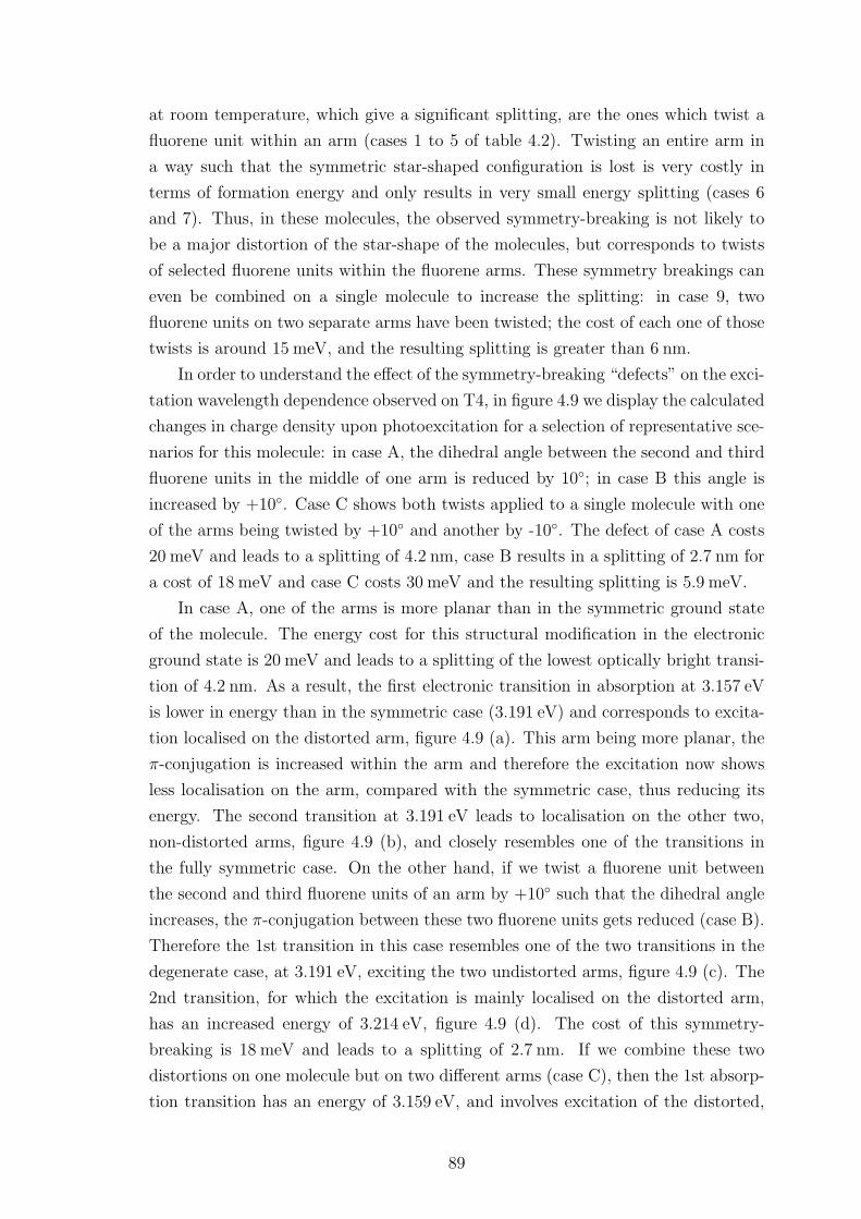
at room temperature, which give a significant splitting, are the ones which twist a

fluorene unit within an arm (cases 1 to 5 of table 4.2). Twisting an entire arm in

a way such that the symmetric star-shaped configuration is lost is very costly in

terms of formation energy and only results in very small energy splitting (cases 6

and 7). Thus, in these molecules, the observed symmetry-breaking is not likely to

be a major distortion of the star-shape of the molecules, but corresponds to twists

of selected fluorene units within the fluorene arms. These symmetry breakings can

even be combined on a single molecule to increase the splitting: in case 9, two

fluorene units on two separate arms have been twisted; the cost of each one of those

twists is around 15 meV, and the resulting splitting is greater than 6 nm.

In order to understand the effect of the symmetry-breaking “defects” on the exci-

tation wavelength dependence observed on T4, in figure 4.9 we display the calculated

changes in charge density upon photoexcitation for a selection of representative sce-

narios for this molecule: in case A, the dihedral angle between the second and third

fluorene units in the middle of one arm is reduced by 10; in case B this angle is

increased by +10. Case C shows both twists applied to a single molecule with one

of the arms being twisted by +10 and another by -10. The defect of case A costs

20 meV and leads to a splitting of 4.2 nm, case B results in a splitting of 2.7 nm for

a cost of 18 meV and case C costs 30 meV and the resulting splitting is 5.9 meV.

In case A, one of the arms is more planar than in the symmetric ground state

of the molecule. The energy cost for this structural modification in the electronic

ground state is 20 meV and leads to a splitting of the lowest optically bright transi-

tion of 4.2 nm. As a result, the first electronic transition in absorption at 3.157 eV

is lower in energy than in the symmetric case (3.191 eV) and corresponds to excita-

tion localised on the distorted arm, figure 4.9 (a). This arm being more planar, the

π-conjugation is increased within the arm and therefore the excitation now shows

less localisation on the arm, compared with the symmetric case, thus reducing its

energy. The second transition at 3.191 eV leads to localisation on the other two,

non-distorted arms, figure 4.9 (b), and closely resembles one of the transitions in

the fully symmetric case. On the other hand, if we twist a fluorene unit between

the second and third fluorene units of an arm by +10 such that the dihedral angle

increases, the π-conjugation between these two fluorene units gets reduced (case B).

Therefore the 1st transition in this case resembles one of the two transitions in the

degenerate case, at 3.191 eV, exciting the two undistorted arms, figure 4.9 (c). The

2nd transition, for which the excitation is mainly localised on the distorted arm,

has an increased energy of 3.214 eV, figure 4.9 (d). The cost of this symmetry-

breaking is 18 meV and leads to a splitting of 2.7 nm. If we combine these two

distortions on one molecule but on two different arms (case C), then the 1st absorp-

tion transition has an energy of 3.159 eV, and involves excitation of the distorted,

89

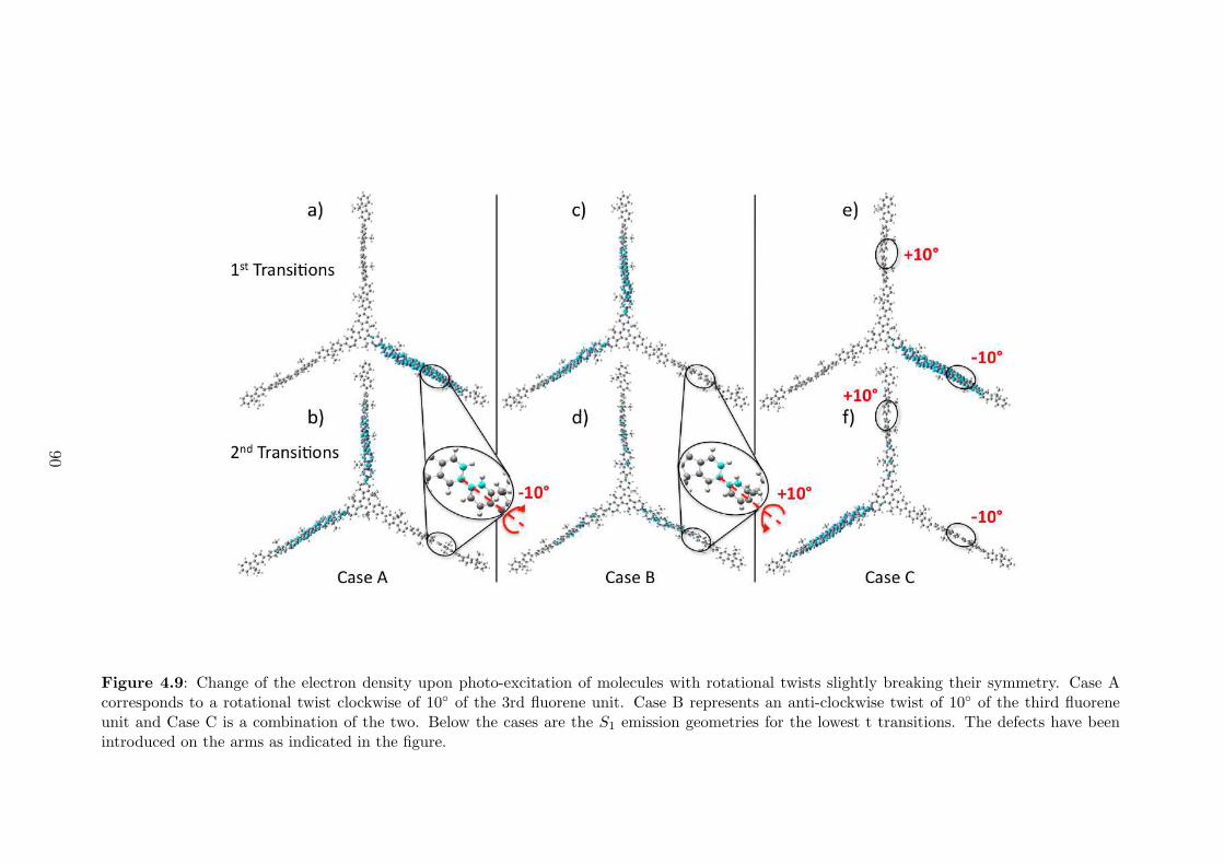
Figure 4.9: Change of the electron density upon photo-excitation of molecules with rotational twists slightly breaking their symmetry. Case Acorresponds to a rotational twist clockwise of 10 of the 3rd fluorene unit. Case B represents an anti-clockwise twist of 10 of the third fluoreneunit and Case C is a combination of the two. Below the cases are the S1 emission geometries for the lowest t transitions. The defects have beenintroduced on the arms as indicated in the figure.

90

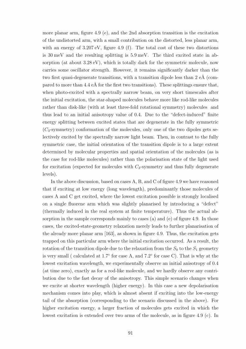
more planar arm, figure 4.9 (e), and the 2nd absorption transition is the excitation

of the undistorted arm, with a small contribution on the distorted, less planar arm,

with an energy of 3.207 eV, figure 4.9 (f). The total cost of these two distortions

is 30 meV and the resulting splitting is 5.9 meV. The third excited state in ab-

sorption (at about 3.28 eV), which is totally dark for the symmetric molecule, now

carries some oscillator strength. However, it remains significantly darker than the

two first quasi-degenerate transitions, with a transition dipole less than 2 eA (com-

pared to more than 4.4 eA for the first two transitions). These splittings ensure that,

when photo-excited with a spectrally narrow beam, on very short timescales after

the initial excitation, the star-shaped molecules behave more like rod-like molecules

rather than disk-like (with at least three-fold rotational symmetry) molecules and

thus lead to an initial anisotropy value of 0.4. Due to the “defect-induced” finite

energy splitting between excited states that are degenerate in the fully symmetric

(C3-symmetry) conformation of the molecules, only one of the two dipoles gets se-

lectively excited by the spectrally narrow light beam. Then, in contrast to the fully

symmetric case, the initial orientation of the transition dipole is to a large extent

determined by molecular properties and spatial orientation of the molecules (as is

the case for rod-like molecules) rather than the polarisation state of the light used

for excitation (expected for molecules with C3-symmetry and thus fully degenerate

levels).

In the above discussion, based on cases A, B, and C of figure 4.9 we have reasoned

that if exciting at low energy (long wavelength), predominantly those molecules of

cases A and C get excited, where the lowest excitation possible is strongly localised

on a single fluorene arm which was slightly planarised by introducing a “defect”

(thermally induced in the real system at finite temperature). Thus the actual ab-

sorption in the sample corresponds mainly to cases (a) and (e) of figure 4.9. In those

cases, the excited-state-geometry relaxation merely leads to further planarisation of

the already more planar arm [163], as shown in figure 4.9. Thus, the excitation gets

trapped on this particular arm where the initial excitation occurred. As a result, the

rotation of the transition dipole due to the relaxation from the S0 to the S1 geometry

is very small ( calculated at 1.7 for case A, and 7.2 for case C). That is why at the

lowest excitation wavelength, we experimentally observe an initial anisotropy of 0.4

(at time zero), exactly as for a rod-like molecule, and we hardly observe any contri-

bution due to the fast decay of the anisotropy. This simple scenario changes when

we excite at shorter wavelength (higher energy). In this case a new depolarisation

mechanism comes into play, which is almost absent if exciting into the low-energy

tail of the absorption (corresponding to the scenario discussed in the above). For

higher excitation energy, a larger fraction of molecules gets excited in which the

lowest excitation is extended over two arms of the molecule, as in figure 4.9 (c). In

91

addition, in those molecules, where the lowest excitation is predominantly localised

on one arm only, the next higher-lying transition also gets excited, as in figure 4.9

(b) and (f). In both cases, when the molecule relaxes into its excited state equilib-

rium geometry, the excitation gets localised (trapped) on only one of the arms, as

illustrated in figure 4.9. This process gives rise to significant and fast rotation of the

transition dipole (our calculations giving 30.1). The experimental data indicates

that we observe this relaxation process, which manifests itself as rapid reduction of

the total anisotropy in the sample at early times after the excitation process.

4.5.3 Slower depolarisation component

Now we turn our attention to the slow decay on the 5-8 ps timescale which

we assign to resonant energy transfer between arms. We have calculated the time

constant of Forster energy transfer between the branches in a weak coupling limit,

using the equation presented in Chapter 1:

1

τF orster

=2π

~g |sV |2 , (4.24)

where V is the electronic coupling energy between donor and acceptor chromophores

and s is the dielectric screening of the interaction by the surrounding medium. g is

a spectral overlap between the homogeneous spectral profiles of donor fluorescence

fhom(E) and acceptor absorption ahom(E), which have each been normalised to

unit area on an energy scale, g =∫ Emax

0fhom(E)ahom(E)dE and Emax is the upper

energy of the vibronic progression in S1 ← S0 absorption [43]. We use s = 1/n2 ,

where n = 1.5 is the refractive index of the solvent, which follows from the dipole

approximation, and the measured steady state fluorescence and absorption spectral

profiles assuming that homogeneous broadening dominates at room temperature.

The electronic coupling V can be determined using the DFT calculations. In-

deed, in the ground-state geometry, each of the three arms is interacting with the

other two. Each individual arm has an energy E0 and interacts with a strength V .

Therefore, the Hamiltonian of the system, H, is:

H =

E0 V V

V E0 V

V V E0

. (4.25)

We call ε1, ε2, ε3 the three transition energies of the molecule. They are the

eigenvalues of the Hamiltonian of the molecule, and the quantities calculated by

quantum chemistry. We can easily calculate that ε1 = ε2 = E0−V and ε3 = E0+2V .

Therefore V is determined as V = (ε3−ε1)/3 , where ε1 and ε3 are the transition

energies from ground state to the lowest energy excited state S1 and to the dark

92

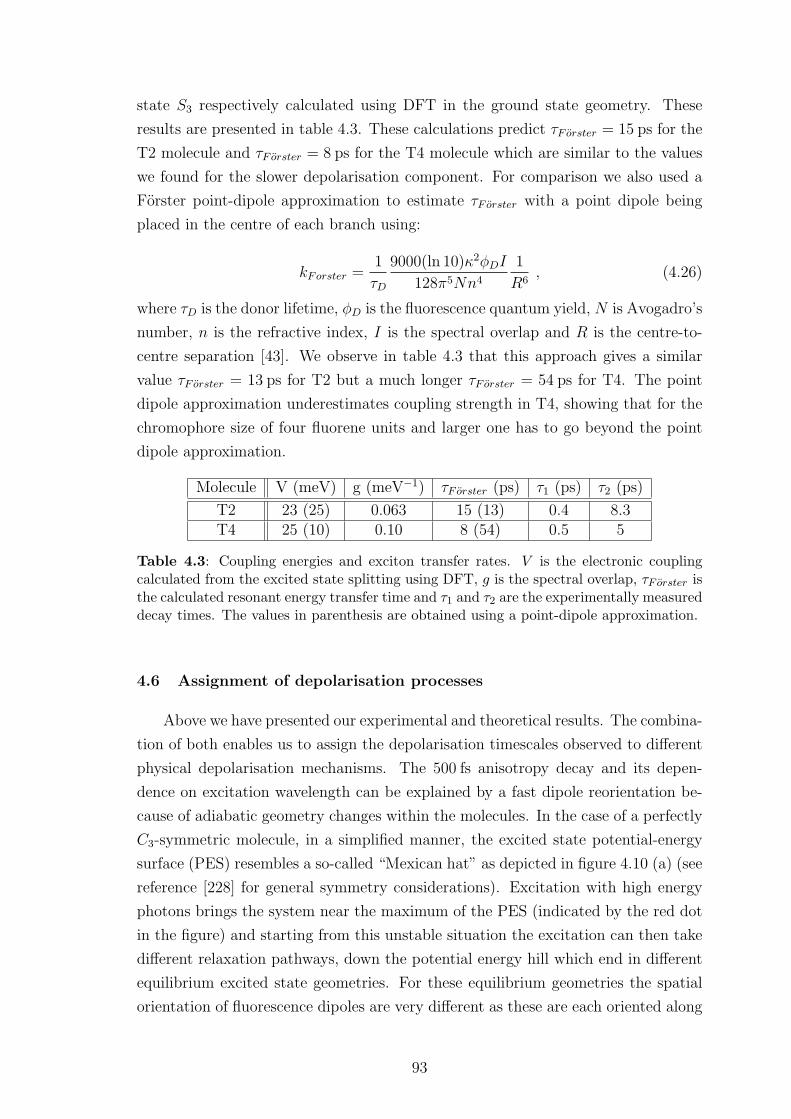
state S3 respectively calculated using DFT in the ground state geometry. These

results are presented in table 4.3. These calculations predict τF orster = 15 ps for the

T2 molecule and τF orster = 8 ps for the T4 molecule which are similar to the values

we found for the slower depolarisation component. For comparison we also used a

Forster point-dipole approximation to estimate τF orster with a point dipole being

placed in the centre of each branch using:

kForster =1

τD

9000(ln 10)κ2φDI

128π5Nn4

1

R6, (4.26)

where τD is the donor lifetime, φD is the fluorescence quantum yield, N is Avogadro’s

number, n is the refractive index, I is the spectral overlap and R is the centre-to-

centre separation [43]. We observe in table 4.3 that this approach gives a similar

value τF orster = 13 ps for T2 but a much longer τF orster = 54 ps for T4. The point

dipole approximation underestimates coupling strength in T4, showing that for the

chromophore size of four fluorene units and larger one has to go beyond the point

dipole approximation.

Molecule V (meV) g (meV−1) τF orster (ps) τ1 (ps) τ2 (ps)

T2 23 (25) 0.063 15 (13) 0.4 8.3T4 25 (10) 0.10 8 (54) 0.5 5

Table 4.3: Coupling energies and exciton transfer rates. V is the electronic couplingcalculated from the excited state splitting using DFT, g is the spectral overlap, τF orster isthe calculated resonant energy transfer time and τ1 and τ2 are the experimentally measureddecay times. The values in parenthesis are obtained using a point-dipole approximation.

4.6 Assignment of depolarisation processes

Above we have presented our experimental and theoretical results. The combina-

tion of both enables us to assign the depolarisation timescales observed to different

physical depolarisation mechanisms. The 500 fs anisotropy decay and its depen-

dence on excitation wavelength can be explained by a fast dipole reorientation be-

cause of adiabatic geometry changes within the molecules. In the case of a perfectly

C3-symmetric molecule, in a simplified manner, the excited state potential-energy

surface (PES) resembles a so-called “Mexican hat” as depicted in figure 4.10 (a) (see

reference [228] for general symmetry considerations). Excitation with high energy

photons brings the system near the maximum of the PES (indicated by the red dot

in the figure) and starting from this unstable situation the excitation can then take

different relaxation pathways, down the potential energy hill which end in different

equilibrium excited state geometries. For these equilibrium geometries the spatial

orientation of fluorescence dipoles are very different as these are each oriented along

93

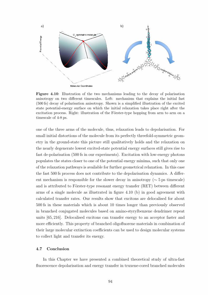
Figure 4.10: Illustration of the two mechanisms leading to the decay of polarisationanisotropy on two different timescales. Left: mechanism that explains the initial fast(500 fs) decay of polarisation anisotropy. Shown is a simplified illustration of the excitedstate potential-energy surface on which the initial relaxation takes place right after theexcitation process. Right: illustration of the Forster-type hopping from arm to arm on atimescale of 4-8 ps.

one of the three arms of the molecule, thus, relaxation leads to depolarisation. For

small initial distortions of the molecule from its perfectly threefold-symmetric geom-

etry in the ground-state this picture still qualitatively holds and the relaxation on

the nearly degenerate lowest excited-state potential energy surfaces still gives rise to

fast de-polarisation (500 fs in our experiments). Excitation with low-energy photons

populates the states closer to one of the potential energy minima, such that only one

of the relaxation pathways is available for further geometrical relaxation. In this case

the fast 500 fs process does not contribute to the depolarisation dynamics. A differ-

ent mechanism is responsible for the slower decay in anisotropy (∼ 5 ps timescale)

and is attributed to Forster-type resonant energy transfer (RET) between different

arms of a single molecule as illustrated in figure 4.10 (b) in good agreement with

calculated transfer rates. Our results show that excitons are delocalised for about

500 fs in these materials which is about 10 times longer than previously observed

in branched conjugated molecules based on amino-styrylbenzene dendrimer repeat

units [65, 216]. Delocalised excitons can transfer energy to an acceptor faster and

more efficiently. This property of branched oligofluorene materials in combination of

their large molecular extinction coefficients can be used to design molecular systems

to collect light and transfer its energy.

4.7 Conclusion

In this Chapter we have presented a combined theoretical study of ultra-fast

fluorescence depolarisation and energy transfer in truxene-cored branched molecules

94

with oligofluorene arms, supported by experiments performed by our collaborators,

and compared the observed dynamics with corresponding linear oligofluorenes. The

anisotropy decay process is found to be bi-exponential with an initial fast 500 fs

localisation followed by a slower 2-8 ps resonant energy transfer between branches.

The fact that it takes 500 fs for exciton localisation to occur can be exploited in the

design of new antennae for efficient light harvesting.

The initially observed polarisation anisotropy value of 0.4 suggests a thermally

induced small symmetry breaking in these nominally symmetric molecules. Calcu-

lations based on density-functional theory confirm that in solution there is enough

thermal energy at room temperature to create a splitting of greater than 5 nm

between the two nominally degenerate lowest optical transitions which allows for

their selective excitation with spectrally narrow light pulses. Our experimental and

theoretical data indicate that after photo-excitation the molecules undergo a two-

stage relaxation energy transfer process. A fast decay of polarisation anisotropy is

found on a 400-500 fs timescale and is attributed to a fast initial relaxation within

the nearly degenerate potential energy surfaces of the lowest excited states. The

relative strength of this process is larger for shorter wavelength excitation, and

is explained by calculations of the excitations generated. The second process is

an excitation-energy independent 5-10 ps decay which we attribute to resonant en-

ergy transfer between different arms of a single molecule. Our results show that

oligofluorene-based materials can support long-lived delocalised excitons which may

mediate efficient energy transfer.

We have so far considered exciton migration in solutions of fluorene based

molecules. However, understanding exciton dynamics processes in films of such

molecules is also of theoretical and practical importance. First, a reliable model for

chromophore interaction is necessary before any further exciton dynamics can be

modelled in a closely packed ensemble of molecules, such as in films. This is the

subject of the next Chapter.

95

Chapter 5

Dipole approximations to calculate intermolecular

interactions

In this Chapter we examine the use and limits of transition dipole theory, both

point- and line-dipole models (used to quantify Forster hopping rates). We then

compare their results with related sets of quantum chemistry calculations for in-

teracting molecules. We demonstrate that the line-dipole model breaks down for

long molecules at separations typical of organic thin-films, whatever the number of

sub-dipoles used. Finally, we present an improved way of distributing the sub-dipole

moments of the line-dipole that overcomes the limits of the usual line-dipole approx-

imation, providing excellent agreement with the quantum chemistry benchmarks.

5.1 Introduction

We have so far investigated excitonic transfer in fluorene-based molecules in

diluted solutions only. However, organic semiconducting thin-films are widely used

in electronic devices such as displays, solar cells, lasers and LEDs. Quantifying the

interactions between excitations in organic chromophores in such thin-films is key

to optimizing the performance of these devices [12, 79, 102, 229]. It has long been

appreciated that the dominant inter-molecular interaction of excitations arises from

a dipole (Forster) coupling [44,230–232].

Due to the complex morphology of the thin films used in such applications [233,

234] it is also crucial to be able to model this dipole coupling on the basis of a simple

dipole-dipole interaction model rather than using an ab initio quantum chemical

method for the whole sample [51,235]. With this in mind, it is interesting to ask what

the range of validity is of such dipole-dipole models and how the dipole moments

and intermolecular distances can be related to quantum chemistry calculations whilst

retaining an accurate description of the interaction. The influence of the geometric

configurations of two molecules has been explored through quantum chemistry [236–

239], but to the best of our knowledge, the limits of the line-dipole model have never

been explored in depth.

This knowledge is a necessary basis for the development of the exciton dynamics

model that we present in Chapter 6, and will also enable future studies which explore

the effect of morphology and phase aggregation on organic thin films. It will also

underpin dynamics studies in relatively large systems, for example, using a quantum

96

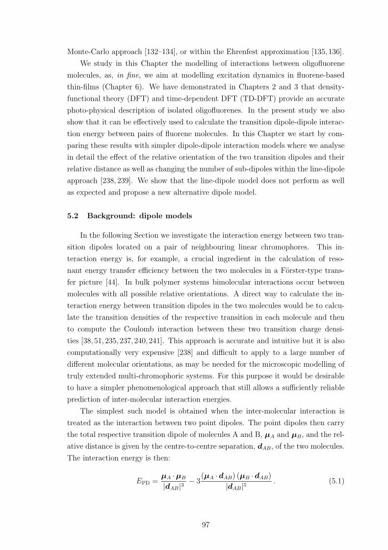
Monte-Carlo approach [132–134], or within the Ehrenfest approximation [135,136].

We study in this Chapter the modelling of interactions between oligofluorene

molecules, as, in fine, we aim at modelling excitation dynamics in fluorene-based

thin-films (Chapter 6). We have demonstrated in Chapters 2 and 3 that density-

functional theory (DFT) and time-dependent DFT (TD-DFT) provide an accurate

photo-physical description of isolated oligofluorenes. In the present study we also

show that it can be effectively used to calculate the transition dipole-dipole interac-

tion energy between pairs of fluorene molecules. In this Chapter we start by com-

paring these results with simpler dipole-dipole interaction models where we analyse

in detail the effect of the relative orientation of the two transition dipoles and their

relative distance as well as changing the number of sub-dipoles within the line-dipole

approach [238, 239]. We show that the line-dipole model does not perform as well

as expected and propose a new alternative dipole model.

5.2 Background: dipole models

In the following Section we investigate the interaction energy between two tran-

sition dipoles located on a pair of neighbouring linear chromophores. This in-

teraction energy is, for example, a crucial ingredient in the calculation of reso-

nant energy transfer efficiency between the two molecules in a Forster-type trans-

fer picture [44]. In bulk polymer systems bimolecular interactions occur between

molecules with all possible relative orientations. A direct way to calculate the in-

teraction energy between transition dipoles in the two molecules would be to calcu-

late the transition densities of the respective transition in each molecule and then

to compute the Coulomb interaction between these two transition charge densi-

ties [38, 51, 235, 237, 240, 241]. This approach is accurate and intuitive but it is also

computationally very expensive [238] and difficult to apply to a large number of

different molecular orientations, as may be needed for the microscopic modelling of

truly extended multi-chromophoric systems. For this purpose it would be desirable

to have a simpler phenomenological approach that still allows a sufficiently reliable

prediction of inter-molecular interaction energies.

The simplest such model is obtained when the inter-molecular interaction is

treated as the interaction between two point dipoles. The point dipoles then carry

the total respective transition dipole of molecules A and B, µA and µB, and the rel-

ative distance is given by the centre-to-centre separation, dAB, of the two molecules.

The interaction energy is then:

EPD =µA ·µB

|dAB|3− 3

(µA ·dAB) (µB ·dAB)

|dAB|5. (5.1)

97

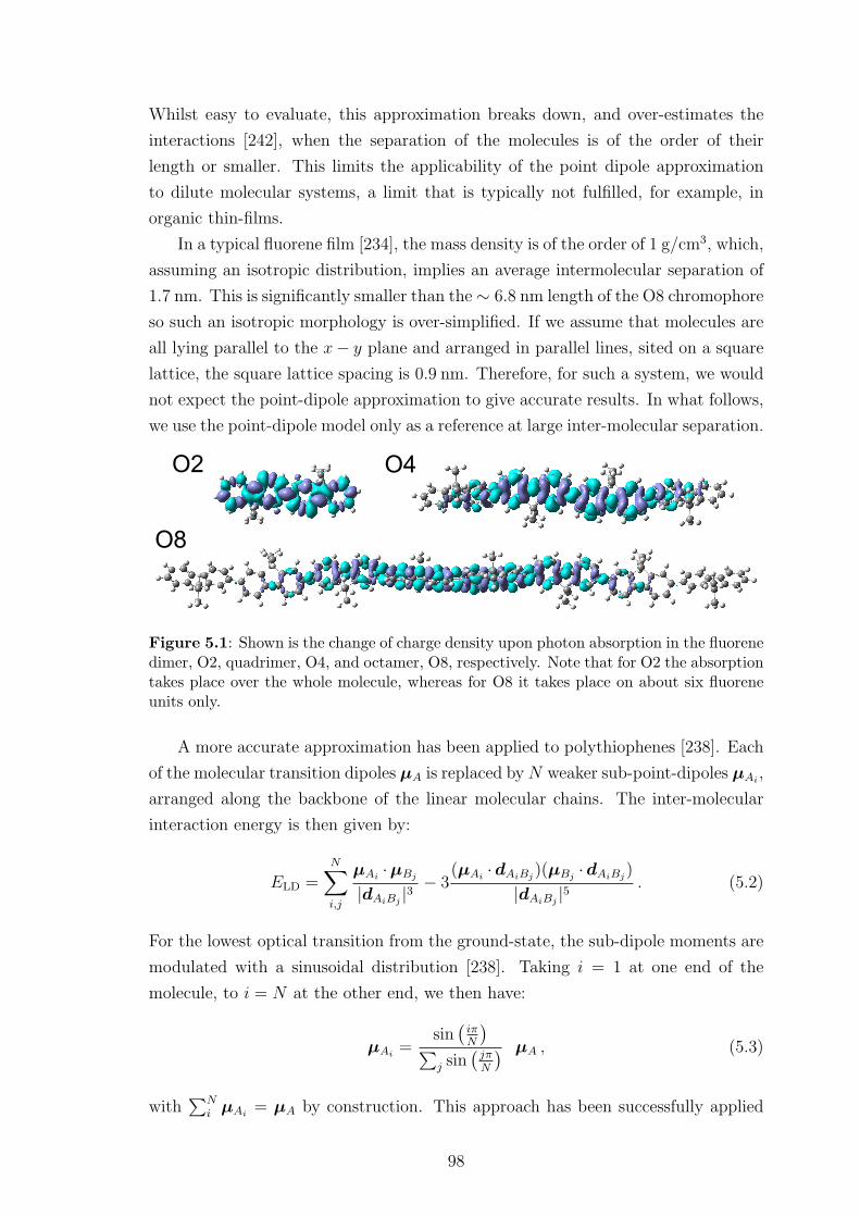
Whilst easy to evaluate, this approximation breaks down, and over-estimates the

interactions [242], when the separation of the molecules is of the order of their

length or smaller. This limits the applicability of the point dipole approximation

to dilute molecular systems, a limit that is typically not fulfilled, for example, in

organic thin-films.

In a typical fluorene film [234], the mass density is of the order of 1 g/cm3, which,

assuming an isotropic distribution, implies an average intermolecular separation of

1.7 nm. This is significantly smaller than the∼ 6.8 nm length of the O8 chromophore

so such an isotropic morphology is over-simplified. If we assume that molecules are

all lying parallel to the x− y plane and arranged in parallel lines, sited on a square

lattice, the square lattice spacing is 0.9 nm. Therefore, for such a system, we would

not expect the point-dipole approximation to give accurate results. In what follows,

we use the point-dipole model only as a reference at large inter-molecular separation.

Figure 5.1: Shown is the change of charge density upon photon absorption in the fluorenedimer, O2, quadrimer, O4, and octamer, O8, respectively. Note that for O2 the absorptiontakes place over the whole molecule, whereas for O8 it takes place on about six fluoreneunits only.

A more accurate approximation has been applied to polythiophenes [238]. Each

of the molecular transition dipoles µA is replaced byN weaker sub-point-dipoles µAi,

arranged along the backbone of the linear molecular chains. The inter-molecular

interaction energy is then given by:

ELD =N∑

i,j

µAi·µBj

|dAiBj|3 − 3

(µAi·dAiBj

)(µBj·dAiBj

)

|dAiBj|5 . (5.2)

For the lowest optical transition from the ground-state, the sub-dipole moments are

modulated with a sinusoidal distribution [238]. Taking i = 1 at one end of the

molecule, to i = N at the other end, we then have:

µAi=

sin(iπN

)∑

j sin(jπN

) µA , (5.3)

with∑N

i µAi= µA by construction. This approach has been successfully applied

98

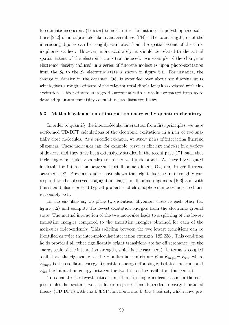
to estimate incoherent (Forster) transfer rates, for instance in polythiophene solu-

tions [242] or in supramolecular nanoassemblies [134]. The total length, L, of the

interacting dipoles can be roughly estimated from the spatial extent of the chro-

mophores studied. However, more accurately, it should be related to the actual

spatial extent of the electronic transition induced. An example of the change in

electronic density induced in a series of fluorene molecules upon photo-excitation

from the S0 to the S1 electronic state is shown in figure 5.1. For instance, the

change in density in the octamer, O8, is extended over about six fluorene units

which gives a rough estimate of the relevant total dipole length associated with this

excitation. This estimate is in good agreement with the value extracted from more

detailed quantum chemistry calculations as discussed below.

5.3 Method: calculation of interaction energies by quantum chemistry

In order to quantify the intermolecular interaction from first principles, we have

performed TD-DFT calculations of the electronic excitations in a pair of two spa-

tially close molecules. As a specific example, we study pairs of interacting fluorene

oligomers. These molecules can, for example, serve as efficient emitters in a variety

of devices, and they have been extensively studied in the recent past [171] such that

their single-molecule properties are rather well understood. We have investigated

in detail the interaction between short fluorene dimers, O2, and longer fluorene

octamers, O8. Previous studies have shown that eight fluorene units roughly cor-

respond to the observed conjugation length in fluorene oligomers [163] and with

this should also represent typical properties of chromophores in polyfluorene chains

reasonably well.

In the calculations, we place two identical oligomers close to each other (cf.

figure 5.2) and compute the lowest excitation energies from the electronic ground

state. The mutual interaction of the two molecules leads to a splitting of the lowest

transition energies compared to the transition energies obtained for each of the

molecules independently. This splitting between the two lowest transitions can be

identified as twice the inter-molecular interaction strength [182,238]. This condition

holds provided all other significantly bright transitions are far off resonance (on the

energy scale of the interaction strength, which is the case here). In terms of coupled

oscillators, the eigenvalues of the Hamiltonian matrix are E = Esingle ± Eint, where

Esingle is the oscillator energy (transition energy) of a single, isolated molecule and

Eint the interaction energy between the two interacting oscillators (molecules).

To calculate the lowest optical transitions in single molecules and in the cou-

pled molecular system, we use linear response time-dependent density-functional

theory (TD-DFT) with the B3LYP functional and 6-31G basis set, which have pre-

99

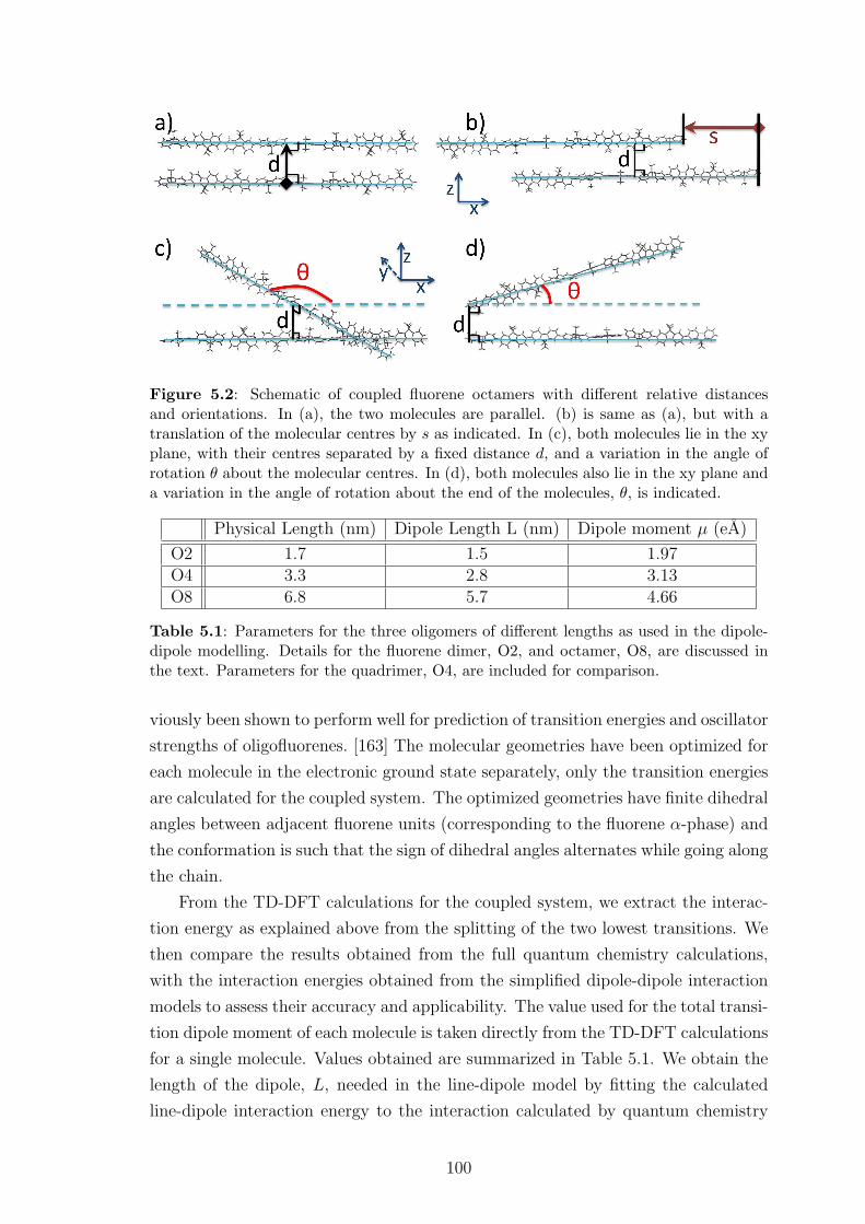
Figure 5.2: Schematic of coupled fluorene octamers with different relative distancesand orientations. In (a), the two molecules are parallel. (b) is same as (a), but with atranslation of the molecular centres by s as indicated. In (c), both molecules lie in the xyplane, with their centres separated by a fixed distance d, and a variation in the angle ofrotation θ about the molecular centres. In (d), both molecules also lie in the xy plane anda variation in the angle of rotation about the end of the molecules, θ, is indicated.

Physical Length (nm) Dipole Length L (nm) Dipole moment µ (eA)

O2 1.7 1.5 1.97O4 3.3 2.8 3.13O8 6.8 5.7 4.66

Table 5.1: Parameters for the three oligomers of different lengths as used in the dipole-dipole modelling. Details for the fluorene dimer, O2, and octamer, O8, are discussed inthe text. Parameters for the quadrimer, O4, are included for comparison.

viously been shown to perform well for prediction of transition energies and oscillator

strengths of oligofluorenes. [163] The molecular geometries have been optimized for

each molecule in the electronic ground state separately, only the transition energies

are calculated for the coupled system. The optimized geometries have finite dihedral

angles between adjacent fluorene units (corresponding to the fluorene α-phase) and

the conformation is such that the sign of dihedral angles alternates while going along

the chain.

From the TD-DFT calculations for the coupled system, we extract the interac-

tion energy as explained above from the splitting of the two lowest transitions. We

then compare the results obtained from the full quantum chemistry calculations,

with the interaction energies obtained from the simplified dipole-dipole interaction

models to assess their accuracy and applicability. The value used for the total transi-

tion dipole moment of each molecule is taken directly from the TD-DFT calculations

for a single molecule. Values obtained are summarized in Table 5.1. We obtain the

length of the dipole, L, needed in the line-dipole model by fitting the calculated

line-dipole interaction energy to the interaction calculated by quantum chemistry

100

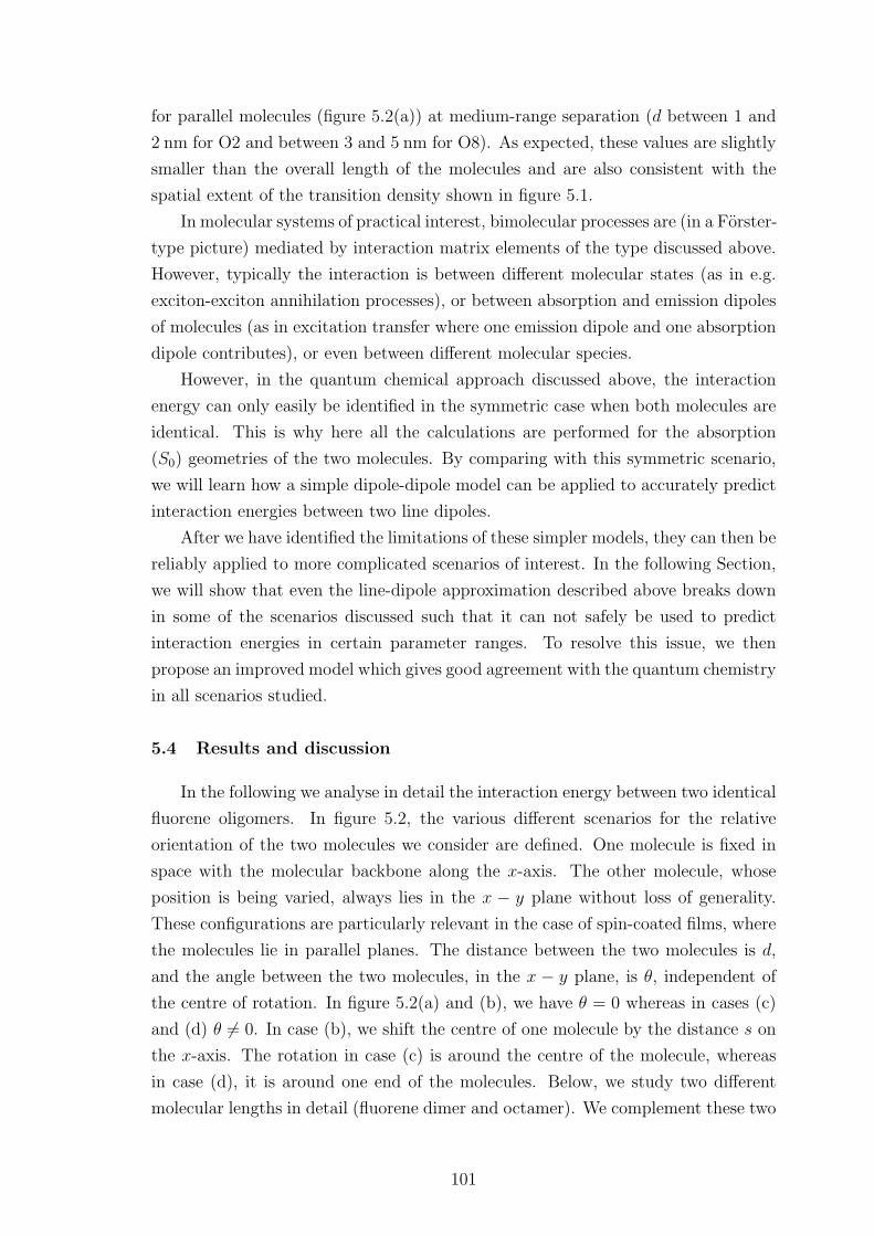
for parallel molecules (figure 5.2(a)) at medium-range separation (d between 1 and

2 nm for O2 and between 3 and 5 nm for O8). As expected, these values are slightly

smaller than the overall length of the molecules and are also consistent with the

spatial extent of the transition density shown in figure 5.1.

In molecular systems of practical interest, bimolecular processes are (in a Forster-

type picture) mediated by interaction matrix elements of the type discussed above.

However, typically the interaction is between different molecular states (as in e.g.

exciton-exciton annihilation processes), or between absorption and emission dipoles

of molecules (as in excitation transfer where one emission dipole and one absorption

dipole contributes), or even between different molecular species.

However, in the quantum chemical approach discussed above, the interaction

energy can only easily be identified in the symmetric case when both molecules are

identical. This is why here all the calculations are performed for the absorption

(S0) geometries of the two molecules. By comparing with this symmetric scenario,

we will learn how a simple dipole-dipole model can be applied to accurately predict

interaction energies between two line dipoles.

After we have identified the limitations of these simpler models, they can then be

reliably applied to more complicated scenarios of interest. In the following Section,

we will show that even the line-dipole approximation described above breaks down

in some of the scenarios discussed such that it can not safely be used to predict

interaction energies in certain parameter ranges. To resolve this issue, we then

propose an improved model which gives good agreement with the quantum chemistry

in all scenarios studied.

5.4 Results and discussion

In the following we analyse in detail the interaction energy between two identical

fluorene oligomers. In figure 5.2, the various different scenarios for the relative

orientation of the two molecules we consider are defined. One molecule is fixed in

space with the molecular backbone along the x-axis. The other molecule, whose

position is being varied, always lies in the x − y plane without loss of generality.

These configurations are particularly relevant in the case of spin-coated films, where

the molecules lie in parallel planes. The distance between the two molecules is d,

and the angle between the two molecules, in the x − y plane, is θ, independent of

the centre of rotation. In figure 5.2(a) and (b), we have θ = 0 whereas in cases (c)

and (d) θ 6= 0. In case (b), we shift the centre of one molecule by the distance s on

the x-axis. The rotation in case (c) is around the centre of the molecule, whereas

in case (d), it is around one end of the molecules. Below, we study two different

molecular lengths in detail (fluorene dimer and octamer). We complement these two

101

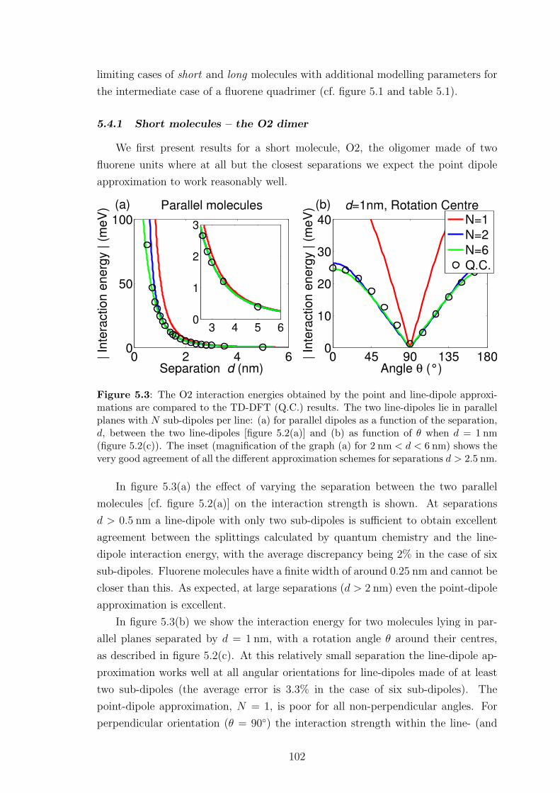
limiting cases of short and long molecules with additional modelling parameters for

the intermediate case of a fluorene quadrimer (cf. figure 5.1 and table 5.1).

5.4.1 Short molecules – the O2 dimer

We first present results for a short molecule, O2, the oligomer made of two

fluorene units where at all but the closest separations we expect the point dipole

approximation to work reasonably well.

Figure 5.3: The O2 interaction energies obtained by the point and line-dipole approxi-mations are compared to the TD-DFT (Q.C.) results. The two line-dipoles lie in parallelplanes with N sub-dipoles per line: (a) for parallel dipoles as a function of the separation,d, between the two line-dipoles [figure 5.2(a)] and (b) as function of θ when d = 1 nm(figure 5.2(c)). The inset (magnification of the graph (a) for 2 nm < d < 6 nm) shows thevery good agreement of all the different approximation schemes for separations d > 2.5 nm.

In figure 5.3(a) the effect of varying the separation between the two parallel

molecules [cf. figure 5.2(a)] on the interaction strength is shown. At separations

d > 0.5 nm a line-dipole with only two sub-dipoles is sufficient to obtain excellent

agreement between the splittings calculated by quantum chemistry and the line-

dipole interaction energy, with the average discrepancy being 2% in the case of six

sub-dipoles. Fluorene molecules have a finite width of around 0.25 nm and cannot be

closer than this. As expected, at large separations (d > 2 nm) even the point-dipole

approximation is excellent.

In figure 5.3(b) we show the interaction energy for two molecules lying in par-

allel planes separated by d = 1 nm, with a rotation angle θ around their centres,

as described in figure 5.2(c). At this relatively small separation the line-dipole ap-

proximation works well at all angular orientations for line-dipoles made of at least

two sub-dipoles (the average error is 3.3% in the case of six sub-dipoles). The

point-dipole approximation, N = 1, is poor for all non-perpendicular angles. For

perpendicular orientation (θ = 90) the interaction strength within the line- (and

102

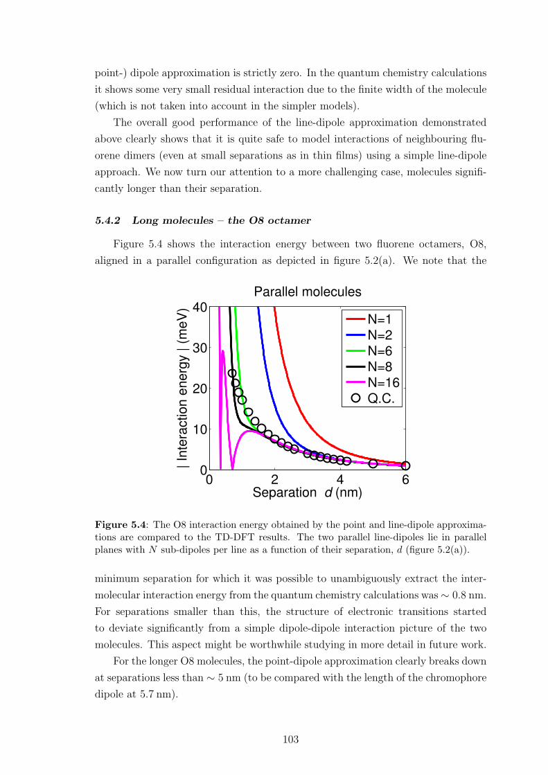
point-) dipole approximation is strictly zero. In the quantum chemistry calculations

it shows some very small residual interaction due to the finite width of the molecule

(which is not taken into account in the simpler models).

The overall good performance of the line-dipole approximation demonstrated

above clearly shows that it is quite safe to model interactions of neighbouring flu-

orene dimers (even at small separations as in thin films) using a simple line-dipole

approach. We now turn our attention to a more challenging case, molecules signifi-

cantly longer than their separation.

5.4.2 Long molecules – the O8 octamer

Figure 5.4 shows the interaction energy between two fluorene octamers, O8,

aligned in a parallel configuration as depicted in figure 5.2(a). We note that the

0 2 4 60

10

20

30

40

Separation d (nm)

| In

tera

ction e

nerg

y | (

meV

)

Parallel molecules

N=1N=2N=6N=8N=16Q.C.

Figure 5.4: The O8 interaction energy obtained by the point and line-dipole approxima-tions are compared to the TD-DFT results. The two parallel line-dipoles lie in parallelplanes with N sub-dipoles per line as a function of their separation, d (figure 5.2(a)).

minimum separation for which it was possible to unambiguously extract the inter-

molecular interaction energy from the quantum chemistry calculations was∼ 0.8 nm.

For separations smaller than this, the structure of electronic transitions started

to deviate significantly from a simple dipole-dipole interaction picture of the two

molecules. This aspect might be worthwhile studying in more detail in future work.

For the longer O8 molecules, the point-dipole approximation clearly breaks down

at separations less than ∼ 5 nm (to be compared with the length of the chromophore

dipole at 5.7 nm).

103

At separations larger than 1 nm, good agreement, having an average discrepancy

of 5%, with the quantum chemistry is found when the line-dipole is made of six sub-

dipoles. However, at smaller separations and when the number of sub-dipoles per line

is at least sixteen, we observe a change of sign of the O8 interaction energy and corre-

spondingly a very poor prediction of values for the interaction strength. (Note that

in the figure we compare the absolute values of the interaction energy). The origin

of this sign change lies in the change in dominant character of the dipole interaction

from repulsive to attractive and can be understood as follows. From equation (5.2)

it is clear that two parallel dipoles [configured as in figure 5.2(a)] will experience a

repulsive interaction (ELD = µA ·µB/|dAB|3), whereas two parallel dipoles arrangedend on will experience an attractive interaction (ELD = −2µA ·µB/|dAB|3).

Physically this attraction arises from the dominant contribution of the two near-

est ends of the dipoles which are oppositely charged. Considering now the line dipole

approximation as used in figure 5.4, at small separations with many sub-dipoles,

the unphysical switch to an attractive interaction arises from the large number of

sub-dipole pairs which are aligned almost end on. Clearly, real molecules do not

possess such a series of very small sub-dipoles such that modelling with very small

sub-dipoles does not reflect the interactions between the molecules in a physically

meaningful fashion. We find that this sign-change behaviour limits the applicability

of the usual line-dipole approximation as for small inter-molecular distance with in-

creasing number of sub-dipoles convergence is not reached at the correct interaction

strength.

In figure 5.5, the separation, d, between the molecules is fixed at 1 or 2 nm,

respectively, with a rotation of angle θ either about the centre or the end of the

molecules.

Seen from above, this results in a +-shaped or an L-shaped configuration, re-

spectively (cf. figure 5.2(c) and (d)).

We observe that when the separation between the molecules is large (2 nm), then

the quantum chemistry and dipole-modelling agree well, as long as we use more than

six sub-dipoles. This is also true for rotation around the end of the molecule. At

smaller separation (1 nm), for line-dipoles made of about six sub-dipoles, the results

agree qualitatively for both rotations, but not quantitatively for the rotation about

the centre. The latter represents the configuration for which the molecules are closest

to each other, such that clearly the limit of the dipole-modelling is reached. In this

case all the dipole results are relatively far from the quantum chemistry results.

At d = 1 nm, it is clear that the line-dipole model starts losing its validity with

worsening quantitative agreement for increasing number of sub-dipoles.

Finally, in figure 5.6, the molecules are parallel (θ = 0), but the centre of one

molecule is shifted with respect to the centre of the other molecule by a distance,

104

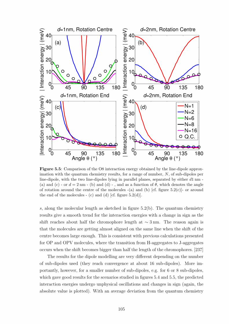
Figure 5.5: Comparison of the O8 interaction energy obtained by the line-dipole approx-imation with the quantum chemistry results, for a range of number, N , of sub-dipoles perline-dipole, with the two line-dipoles lying in parallel planes, separated by either d1 nm -(a) and (c) - or d = 2 nm - (b) and (d) - , and as a function of θ, which denotes the angleof rotation around the centre of the molecules -(a) and (b) [cf. figure 5.2(c)]- or aroundthe end of the molecules - (c) and (d) [cf. figure 5.2(d)].

s, along the molecular length as sketched in figure 5.2(b). The quantum chemistry

results give a smooth trend for the interaction energies with a change in sign as the

shift reaches about half the chromophore length at ∼ 3 nm. The reason again is

that the molecules are getting almost aligned on the same line when the shift of the

centre becomes large enough. This is consistent with previous calculations presented

for OP and OPV molecules, where the transition from H-aggregates to J-aggregates

occurs when the shift becomes bigger than half the length of the chromophores. [237]

The results for the dipole modelling are very different depending on the number

of sub-dipoles used (they reach convergence at about 16 sub-dipoles). More im-

portantly, however, for a smaller number of sub-dipoles, e.g. for 6 or 8 sub-dipoles,

which gave good results for the scenarios studied in figures 5.4 and 5.5, the predicted

interaction energies undergo unphysical oscillations and changes in sign (again, the

absolute value is plotted). With an average deviation from the quantum chemistry

105

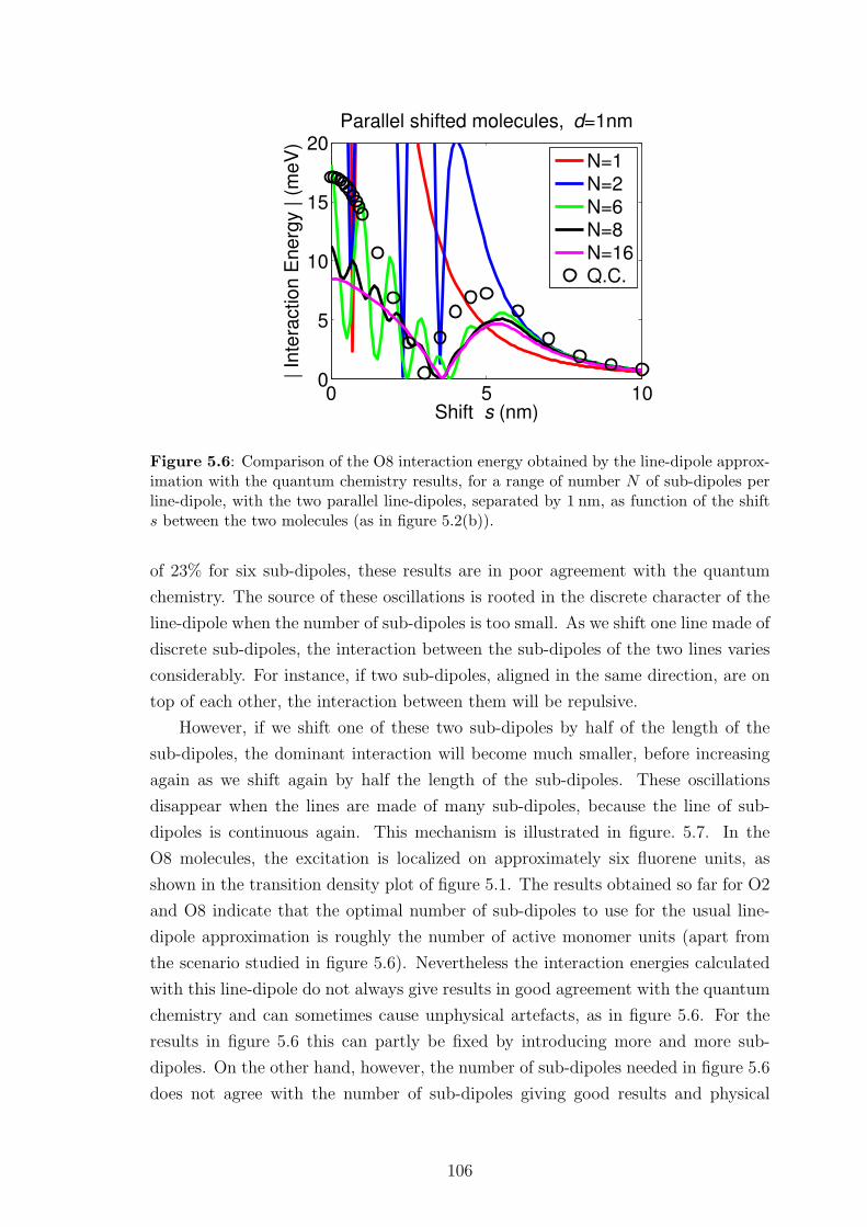
0 5 100

5

10

15

20

Shift s (nm)

| In

tera

ctio

n E

ne

rgy | (

me

V)

Parallel shifted molecules, d=1nm

N=1N=2N=6N=8N=16Q.C.

Figure 5.6: Comparison of the O8 interaction energy obtained by the line-dipole approx-imation with the quantum chemistry results, for a range of number N of sub-dipoles perline-dipole, with the two parallel line-dipoles, separated by 1 nm, as function of the shifts between the two molecules (as in figure 5.2(b)).

of 23% for six sub-dipoles, these results are in poor agreement with the quantum

chemistry. The source of these oscillations is rooted in the discrete character of the

line-dipole when the number of sub-dipoles is too small. As we shift one line made of

discrete sub-dipoles, the interaction between the sub-dipoles of the two lines varies

considerably. For instance, if two sub-dipoles, aligned in the same direction, are on

top of each other, the interaction between them will be repulsive.

However, if we shift one of these two sub-dipoles by half of the length of the

sub-dipoles, the dominant interaction will become much smaller, before increasing

again as we shift again by half the length of the sub-dipoles. These oscillations

disappear when the lines are made of many sub-dipoles, because the line of sub-

dipoles is continuous again. This mechanism is illustrated in figure. 5.7. In the

O8 molecules, the excitation is localized on approximately six fluorene units, as

shown in the transition density plot of figure 5.1. The results obtained so far for O2

and O8 indicate that the optimal number of sub-dipoles to use for the usual line-

dipole approximation is roughly the number of active monomer units (apart from

the scenario studied in figure 5.6). Nevertheless the interaction energies calculated

with this line-dipole do not always give results in good agreement with the quantum

chemistry and can sometimes cause unphysical artefacts, as in figure 5.6. For the

results in figure 5.6 this can partly be fixed by introducing more and more sub-

dipoles. On the other hand, however, the number of sub-dipoles needed in figure 5.6

does not agree with the number of sub-dipoles giving good results and physical

106

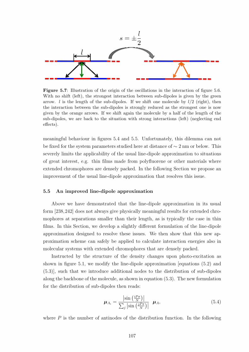
Figure 5.7: Illustration of the origin of the oscillations in the interaction of figure 5.6.With no shift (left), the strongest interaction between sub-dipoles is given by the greenarrow. l is the length of the sub-dipoles. If we shift one molecule by l/2 (right), thenthe interaction between the sub-dipoles is strongly reduced as the strongest one is nowgiven by the orange arrows. If we shift again the molecule by a half of the length of thesub-dipoles, we are back to the situation with strong interactions (left) (neglecting endeffects).

meaningful behaviour in figures 5.4 and 5.5. Unfortunately, this dilemma can not

be fixed for the system parameters studied here at distance of ∼ 2 nm or below. This

severely limits the applicability of the usual line-dipole approximation to situations

of great interest, e.g. thin films made from polyfluorene or other materials where

extended chromophores are densely packed. In the following Section we propose an

improvement of the usual line-dipole approximation that resolves this issue.

5.5 An improved line-dipole approximation

Above we have demonstrated that the line-dipole approximation in its usual

form [238,242] does not always give physically meaningful results for extended chro-

mophores at separations smaller than their length, as is typically the case in thin

films. In this Section, we develop a slightly different formulation of the line-dipole

approximation designed to resolve these issues. We then show that this new ap-

proximation scheme can safely be applied to calculate interaction energies also in

molecular systems with extended chromophores that are densely packed.

Instructed by the structure of the density changes upon photo-excitation as

shown in figure 5.1, we modify the line-dipole approximation [equations (5.2) and

(5.3)], such that we introduce additional nodes to the distribution of sub-dipoles

along the backbone of the molecule, as shown in equation (5.3). The new formulation

for the distribution of sub-dipoles then reads:

µAi=

∣∣sin(iPπN

)∣∣∑

j

∣∣sin(jPπN

)∣∣ µA, (5.4)

where P is the number of antinodes of the distribution function. In the following

107

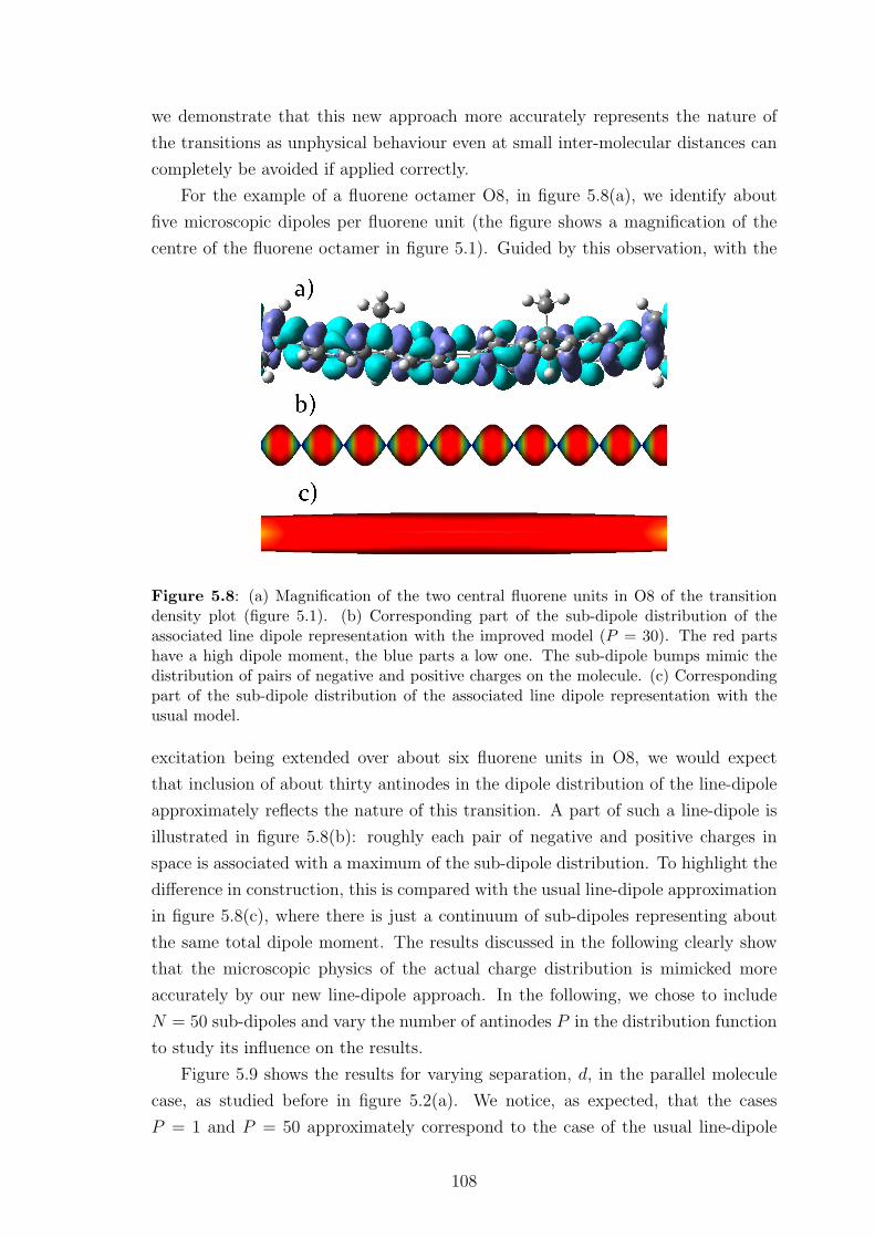
we demonstrate that this new approach more accurately represents the nature of

the transitions as unphysical behaviour even at small inter-molecular distances can

completely be avoided if applied correctly.

For the example of a fluorene octamer O8, in figure 5.8(a), we identify about

five microscopic dipoles per fluorene unit (the figure shows a magnification of the

centre of the fluorene octamer in figure 5.1). Guided by this observation, with the

Figure 5.8: (a) Magnification of the two central fluorene units in O8 of the transitiondensity plot (figure 5.1). (b) Corresponding part of the sub-dipole distribution of theassociated line dipole representation with the improved model (P = 30). The red partshave a high dipole moment, the blue parts a low one. The sub-dipole bumps mimic thedistribution of pairs of negative and positive charges on the molecule. (c) Correspondingpart of the sub-dipole distribution of the associated line dipole representation with theusual model.

excitation being extended over about six fluorene units in O8, we would expect

that inclusion of about thirty antinodes in the dipole distribution of the line-dipole

approximately reflects the nature of this transition. A part of such a line-dipole is

illustrated in figure 5.8(b): roughly each pair of negative and positive charges in

space is associated with a maximum of the sub-dipole distribution. To highlight the

difference in construction, this is compared with the usual line-dipole approximation

in figure 5.8(c), where there is just a continuum of sub-dipoles representing about

the same total dipole moment. The results discussed in the following clearly show

that the microscopic physics of the actual charge distribution is mimicked more

accurately by our new line-dipole approach. In the following, we chose to include

N = 50 sub-dipoles and vary the number of antinodes P in the distribution function

to study its influence on the results.

Figure 5.9 shows the results for varying separation, d, in the parallel molecule

case, as studied before in figure 5.2(a). We notice, as expected, that the cases

P = 1 and P = 50 approximately correspond to the case of the usual line-dipole

108

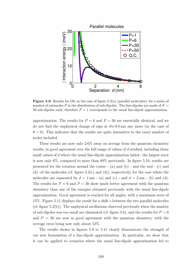
0 2 4 60

10

20

30

Separation d (nm)

| In

tera

ctio

n e

ne

rgy | (

me

V)

Parallel molecules

P=1P=6P=30P=50Q.C.

Figure 5.9: Results for O8, in the case of figure 5.2(a) (parallel molecules), for a series ofnumber of antinodes P in the distribution of sub-dipoles. The line-dipoles are made ofN =50 sub-dipoles each, therefore P = 1 corresponds to the usual line-dipole approximation.

approximation. The results for P = 6 and P = 30 are essentially identical, and we

do not find the unphysical change of sign at d≈ 0.8 nm any more (in the case of

θ = 0). This indicates that the results are quite insensitive to the exact number of

nodes included.

These results are now only 2.6% away on average from the quantum chemistry

results, in good agreement over the full range of values of d studied, including those

small values of d where the usual line-dipole approximation failed - the largest error

is now only 6%, compared to more than 80% previously. In figure 5.10, results are

presented for the rotation around the centre - (a) and (b) - and the end - (c) and

(d) -of the molecules (cf. figure 5.2(c) and (d)), respectively, for the case where the

molecules are separated by d = 1 nm - (a) and (c) - and d = 2 nm - (b) and (d).

The results for P = 6 and P = 30 show much better agreement with the quantum

chemistry than any of the energies obtained previously with the usual line-dipole

approximation. Good agreement is reached for all angles, with a maximum error of

15%. Figure 5.11 displays the result for a shift s between the two parallel molecules

(cf. figure 5.2(b)). The unphysical oscillations observed previously when the number

of sub-dipoles was too small are eliminated (cf. figure 5.6), and the results for P = 6

and P = 30 are now in good agreement with the quantum chemistry, with the

average error being now only about 12%.

The results shown in figures 5.9 to 5.11 clearly demonstrate the strength of

our new formulation of a line-dipole approximation. In particular, we show that

it can be applied to scenarios where the usual line-dipole approximation led to

109

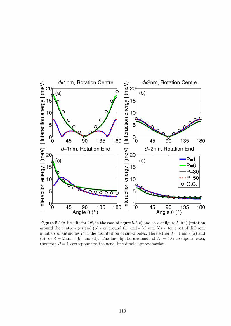
Figure 5.10: Results for O8, in the case of figure 5.2(c) and case of figure 5.2(d) (rotationaround the centre - (a) and (b) - or around the end - (c) and (d) -, for a set of differentnumbers of antinodes P in the distribution of sub-dipoles. Here either d = 1 nm - (a) and(c)- or d = 2 nm - (b) and (d). The line-dipoles are made of N = 50 sub-dipoles each,therefore P = 1 corresponds to the usual line-dipole approximation.

110

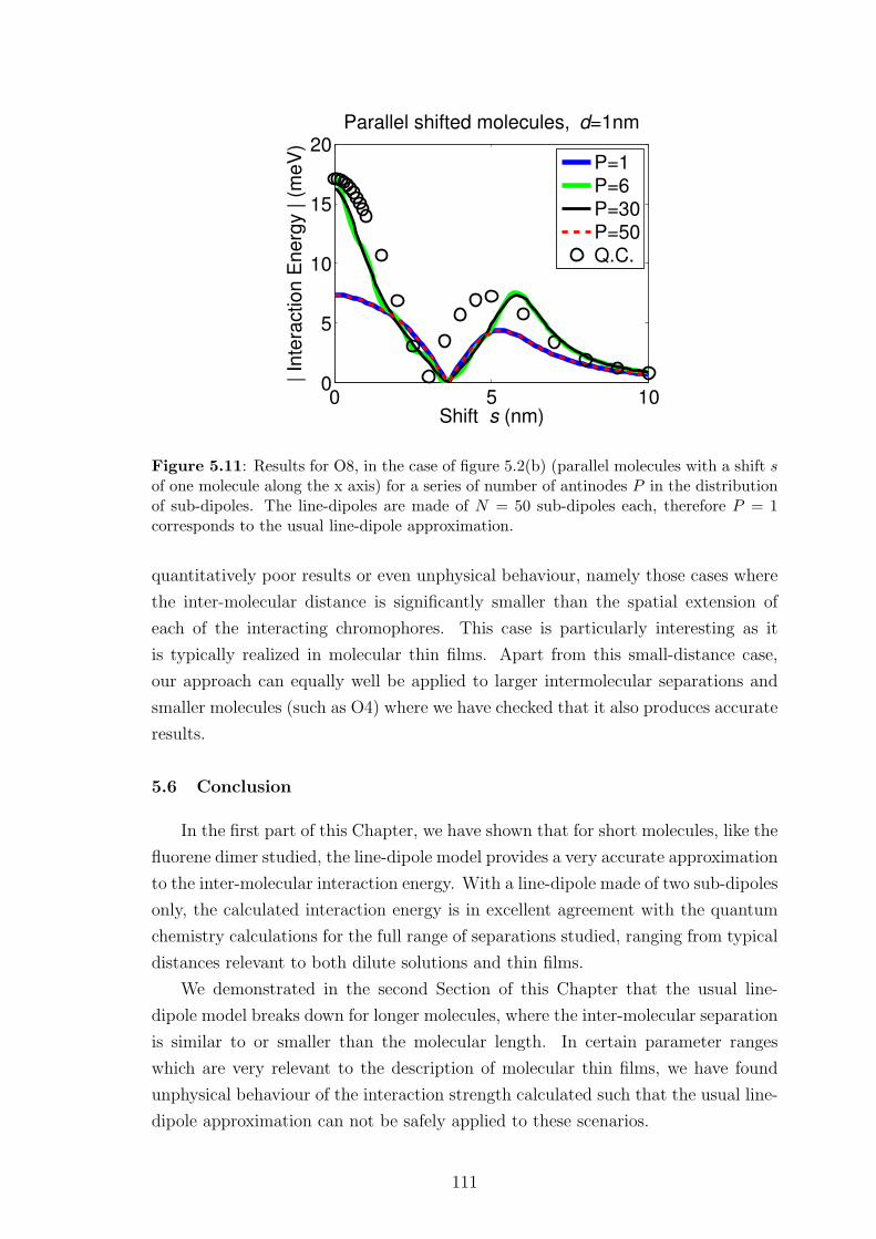
0 5 100

5

10

15

20

Shift s (nm)

| In

tera

ctio

n E

ne

rgy | (

me

V)

Parallel shifted molecules, d=1nm

P=1P=6P=30P=50Q.C.

Figure 5.11: Results for O8, in the case of figure 5.2(b) (parallel molecules with a shift sof one molecule along the x axis) for a series of number of antinodes P in the distributionof sub-dipoles. The line-dipoles are made of N = 50 sub-dipoles each, therefore P = 1corresponds to the usual line-dipole approximation.

quantitatively poor results or even unphysical behaviour, namely those cases where

the inter-molecular distance is significantly smaller than the spatial extension of

each of the interacting chromophores. This case is particularly interesting as it

is typically realized in molecular thin films. Apart from this small-distance case,

our approach can equally well be applied to larger intermolecular separations and

smaller molecules (such as O4) where we have checked that it also produces accurate

results.

5.6 Conclusion

In the first part of this Chapter, we have shown that for short molecules, like the

fluorene dimer studied, the line-dipole model provides a very accurate approximation

to the inter-molecular interaction energy. With a line-dipole made of two sub-dipoles

only, the calculated interaction energy is in excellent agreement with the quantum

chemistry calculations for the full range of separations studied, ranging from typical

distances relevant to both dilute solutions and thin films.

We demonstrated in the second Section of this Chapter that the usual line-

dipole model breaks down for longer molecules, where the inter-molecular separation

is similar to or smaller than the molecular length. In certain parameter ranges

which are very relevant to the description of molecular thin films, we have found

unphysical behaviour of the interaction strength calculated such that the usual line-

dipole approximation can not be safely applied to these scenarios.

111

In the last part of this Chapter we presented a new formulation of the line-

dipole approximation which enables us to overcome these limitations. This new

formulation of the interaction of transition dipoles includes nodes in the distribution

of sub-dipole moments in addition to the simple line-dipole approximation. Results

obtained are then in excellent quantitative agreement with the TD-DFT calculations

for all spatial separations and relative orientations considered.

This new line-dipole model enables us to calculate efficiently and accurately

the interactions between pairs of oligofluorenes. In the next Chapter we present a

microscopic model taking advantage of this improved line-dipole approximation to

simulate accurately the exciton dynamics in polyfluorene films.

112

Chapter 6

A microscopic model of exciton dynamics in

polyfluorene films

In this Chapter we present a combined experimental and theoretical study of

exciton dynamics in polyfluorene films. The observed sub-picosecond fluorescence

anisotropy decay leads us to use the efficient and reliable chromophore interaction

energy calculation method presented in Chapter 5 for the construction of a micro-

scopic dynamics model. This model demonstrates that if film morphology, both

physical and spectral, is properly accounted for, dipole mediated hopping is suffi-

cient to fully explain the observed sub-picosecond dynamics.

6.1 Introduction

Understanding the photo-physics of ensembles of organic semiconductor molecules

is essential if progress towards more efficient and functional devices is to be made

[243–246]. We have shown in Chapter 1 that one fundamental process that un-

derpins the operation of devices is energy transfer through the material, and that

numerous research efforts are still ongoing to fully understand the fundamental

energy transfer processes. Forster first proposed his incoherent energy transfer

theory more than six decades ago [44]. Since then many extensions to this the-

ory have been developed [46, 47, 54–58], and new theories to describe coherent or

partially-coherent energy transfer have also emerged [42, 65–68] - we give a more

detailed overview of these theories in Chapter 1. In devices, the combined addi-

tional influence of, amongst others, sample morphology [233, 234], molecular con-

formations [37, 247, 248], packing and traps [71, 249], exciton hopping and exciton

annihilation makes the problem of device optimization even more challenging, as

it involves a wide range of energies, timespans and difficult to access parameters.

Unpicking one from another is challenging and requires a combination of both exper-

imental and theoretical approaches. Simulations of large-scale systems are usually

conducted in the framework of a Monte-Carlo approach [128,132–134] or a Master-

Equation-type approach [125, 136, 250–252], whereas experiments often investigate

spectral- and time-resolved photo-luminescence decay [14, 234, 253] or pump-probe

spectroscopy [14, 254] to monitor ultra-fast photo-physics. Rather than investigat-

ing the dynamics of excitons in organic systems, many of the theoretical simulations

model charge-separated excitations [126, 127, 129–131, 255], as this is particularly

113

relevant to devices such as photovoltaics and LEDs. However, even in these sys-

tems, knowledge of exciton dynamics is fundamental to understand and predict the

early-time dynamics of the solar generated excitations.

We have studied ultra-fast exciton dynamics in solutions of fluorene-based star-

shaped molecules and of oligofluorenes in Chapter 4. In this Chapter, we focus on

films of polyfluorene (PF8). Using fluorescence ultra-fast anisotropy experiments,

as in Chapter 4, we measure how long the initial photo-induced dipole orientation

survives, and infer from that a hopping time for excitonic excitations. As we shall

show, an analysis based on simple mean field hopping rates fails to account for

the measured sub-picosecond anisotropy decay. We therefore develop a detailed

microscopic model of the dynamical processes involved which is able to correctly

describe the experimental findings. Finally, we use this model to further explore the

detailed physics underlying these results and answer a number of open questions

about the importance of inhomogeneous versus homogeneous broadening, exciton

localization, and the typical number of hops an exciton undergoes before becoming

localized.

6.2 Experiments: fluorescence anisotropy in PFO films

All the experiments presented in this Chapter have been performed by our col-

laborators at the university of St Andrews.

6.2.1 Experimental methodology

Films of PF8 were prepared using a spin-coating technique. It was ensured that

only glassy phase polyfluorene was formed. The films were pumped by a 100 fs

(full-width half-maximum) laser pump pulse at an excitation wavelength of 400 nm.

Ultrafast luminescence was measured at a detection wavelength of 475 nm. Fluo-

rescence dynamics parallel (I‖) and perpendicular (I⊥) to the excitation were mea-

sured. The instrument response function (IRF) was also recorded, and was found to

be 380 fs FWHM. Having measured fluorescence dynamics parallel and perpendic-

ular to the excitation polarisation the anisotropy can be reconstructed, where the

anisotropy, r, is defined as in Chapter 4:

r =I‖ − I⊥I‖ + 2I⊥

. (6.1)

The “magic angle” (polarisation-independent fluorescence dynamics) is also defined

in the same way as in Chapter 4: m = (I‖ + 2I⊥)/3.

As in Chapter 4, fitting of the depolarisation kinetics was performed using the

impulse reconvolution method [226] which enables deconvolution of the instrument

114

response function from the decay. The fitting methodology involves convolving a

sum of exponentials with the IRF and then fitting the results with the magic angle

m. The best-fit for the magic angle kinetics can then be convolved with a trial

function representing the depolarisation and also convolved with the IRF. Iteration

of the trial function to give a good fit to the numerator of equation (6.1) (the so-

called difference fit) enables the depolarisation to be fitted with full account taken

of the instrument response function.

6.2.2 Experimental results

The ultra-fast fluorescence kinetics in the polyfluorene file (PF8) are shown in

figure 6.1(a). In the “magic angle” kinetics of the photoluminescence (PL) at the

475 nm (on the 0-2 vibronic) peak we are able to fit fast and slow exponential rise-

times of 200 fs and 2 ps, with 0.76 amplitude assigned to the fast component and

0.19 assigned to the slow, with the remaining 0.05 contribution essentially instan-

taneous following the pump. As expected, on the red-side of the PL spectrum we

observe an increase in PL intensity over the first few picoseconds, a rise attributed

to electronic and geometry relaxation (e.g. bond lengths, torsional angles). These

processes, however, cannot easily be disentangled from the energy transfer between

chromophores (on or between polymer chains) that is occurring when just looking

at the ensemble magic angle dynamics alone. Consequently, we have monitored the

depolarisation of the fluorescence by recording fluorescence kinetics parallel and per-

pendicular to the laser field to obtain information on the change in the angle of the

dipole moment of the exciton on an ultra-fast timescale. The fluorescence anisotropy

of PF8 at a detection wavelength of 475 nm is shown in figure 6.1(b). We have cho-

sen a detection wavelength on the red-side of the PL spectrum to ensure that there

is absolutely no contamination of the recorded signal with the excitation laser field

or any prompt higher energy emission from PF8. The instrument response does not

enable us to resolve the initial anisotropy of 0.4 that we might expect (as demon-

strated in Chapter 4); instead, around t 6 0, we observe noisy anisotropy values

as the intensity recorded is very low. Using the anisotropy fitting procedure as de-

scribed in the experimental methodology we find that the depolarisation fits to time

constants of 680 fs and 5 ps with depolarisation amplitudes (i.e. loss of anisotropy)

of 0.24 and 0.09 respectively. These values are considerably different from the fitted

time constants of the magic angle kinetics and show that as well as electronic and

geometric relaxation, dipole reorientation is occurring on fast and slower timescales.

To the best of our knowledge this is the first time that the ultra-fast fluorescence

depolarisation has been investigated in films of polyfluorene. The observation of

such fast depolarisation is not necessarily unexpected in films of conjugated poly-

mers (for instance sub-picosecond fluorescence anisotropy decay has been measured

115

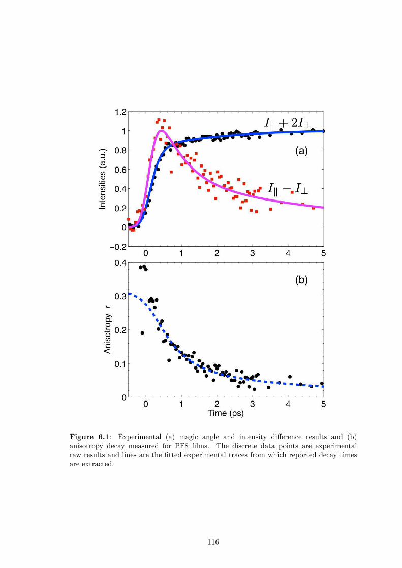
Figure 6.1: Experimental (a) magic angle and intensity difference results and (b)anisotropy decay measured for PF8 films. The discrete data points are experimentalraw results and lines are the fitted experimental traces from which reported decay timesare extracted.

116

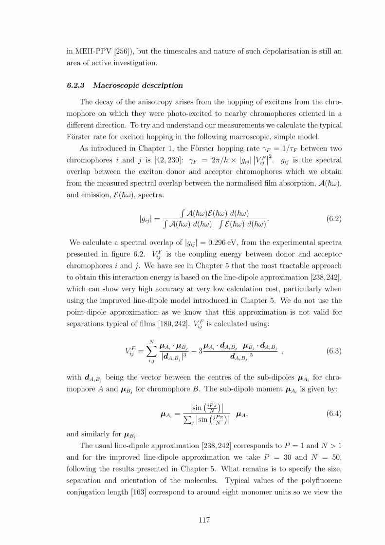
in MEH-PPV [256]), but the timescales and nature of such depolarisation is still an

area of active investigation.

6.2.3 Macroscopic description

The decay of the anisotropy arises from the hopping of excitons from the chro-

mophore on which they were photo-excited to nearby chromophores oriented in a

different direction. To try and understand our measurements we calculate the typical

Forster rate for exciton hopping in the following macroscopic, simple model.

As introduced in Chapter 1, the Forster hopping rate γF = 1/τF between two

chromophores i and j is [42, 230]: γF = 2π/~ × |gij|∣∣V F

ij

∣∣2. gij is the spectral

overlap between the exciton donor and acceptor chromophores which we obtain

from the measured spectral overlap between the normalised film absorption, A(~ω),and emission, E(~ω), spectra.

|gij| =∫A(~ω)E(~ω) d(~ω)∫

A(~ω) d(~ω)∫E(~ω) d(~ω) . (6.2)

We calculate a spectral overlap of |gij| = 0.296 eV, from the experimental spectra

presented in figure 6.2. V Fij is the coupling energy between donor and acceptor

chromophores i and j. We have see in Chapter 5 that the most tractable approach

to obtain this interaction energy is based on the line-dipole approximation [238,242],

which can show very high accuracy at very low calculation cost, particularly when

using the improved line-dipole model introduced in Chapter 5. We do not use the

point-dipole approximation as we know that this approximation is not valid for

separations typical of films [180,242]. V Fij is calculated using:

V Fij =

N∑

i,j

µAi·µBj

|dAiBj|3 − 3

µAi·dAiBj

µBj·dAiBj

|dAiBj|5 , (6.3)

with dAiBjbeing the vector between the centres of the sub-dipoles µAi

for chro-

mophore A and µBjfor chromophore B. The sub-dipole moment µAi

is given by:

µAi=

∣∣sin(iPπN

)∣∣∑

j

∣∣sin(jPπN

)∣∣ µA, (6.4)

and similarly for µBi.

The usual line-dipole approximation [238,242] corresponds to P = 1 and N > 1

and for the improved line-dipole approximation we take P = 30 and N = 50,

following the results presented in Chapter 5. What remains is to specify the size,

separation and orientation of the molecules. Typical values of the polyfluorene

conjugation length [163] correspond to around eight monomer units so we view the

117

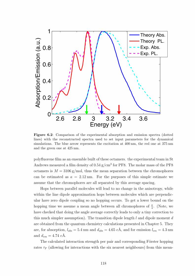
2.6 2.8 3 3.2 3.4 3.60

0.2

0.4

0.6

0.8

1

Energy (eV)

Absorp

tion/E

mis

sio

n (

a.u

.)

Theory Abs.

Theory PL.

Exp. Abs.

Exp. PL.

Figure 6.2: Comparison of the experimental absorption and emission spectra (dottedlines) with the reconstructed spectra used to set input parameters for the dynamicalsimulations. The blue arrow represents the excitation at 400 nm, the red one at 375 nmand the green one at 425 nm.

polyfluorene film as an ensemble built of these octamers. the experimental team in St

Andrews measured a film density of 0.54 g/cm3 for PF8. The molar mass of the PF8

octamers is M = 3106 g/mol, thus the mean separation between the chromophores

can be estimated as a = 2.12 nm. For the purposes of this simple estimate we

assume that the chromophores are all separated by this average spacing.

Hops between parallel molecules will lead to no change in the anisotropy, while

within the line dipole approximation hops between molecules which are perpendic-

ular have zero dipole coupling so no hopping occurs. To get a lower bound on the

hopping time we assume a mean angle between all chromophores of π4. (Note, we

have checked that doing the angle average correctly leads to only a tiny correction to

this much simpler assumption). The transition dipole length l and dipole moment d

are obtained from the quantum chemistry calculations presented in Chapter 5. They

are, for absorption, labs = 5.4 nm and dabs = 4.65 eA, and for emission lem = 4.3 nm

and dem = 4.74 eA.

The calculated interaction strength per pair and corresponding Forster hopping

rates τF (allowing for interactions with the six nearest neighbours) from this mean-

118

Dipole model Interaction per pair (meV) τF (ps)

Line-dipole 5.54 12.1Improved line-dipole 3.97 23.5

Table 6.1: Interaction energies estimates for the simple model, for a pair of chromophoresand for a chromophore interacting with its six closest neighbours, and hopping timesestimates for this last case.

field type model are given in table 6.1. It can be seen that, even using the largest

interaction strength, this mean-behaviour model predicts a hopping time much larger

(twenty times slower) than the experimentally observed 0.68 ps anisotropy decay.

The reason for the failure of this simple intuitive model is that the interactions

which dominate the decay are not well captured in a model based on the average

properties of the film, as we shall see in the next Section.

6.3 Microscopic theory of exciton diffusion in PFO films

6.3.1 The microscopic model

The simple estimate presented above is not able to correctly explain the observed

time-scales for the anisotropy decay in polyfluorene films. Indeed, it underestimates

the decay rate by a factor of over thirty. Therefore we introduce a more detailed

model where the microscopic hopping dynamics and sample geometry are more

accurately captured. This model will allow us to simulate the exciton dynamics in a

large ensemble of chromophores. In what follows we will adopt a number of simple

but sufficient assumptions to avoid the need for “fitting” parameters in such a model.

To this end we use the combined insight from our experimental measurements and

quantum chemistry calculations to obtain all the necessary parameters. In this sense

the model is predictive and not merely a complex fitting procedure.

In this Subsection we introduce this model and its assumptions. Its formalism is

developed in the next Subsection. The choice of parameters, illustrated by, but not

restricted to, the simulation of polyfluorene films, will be the subject of Subsection

6.4.

We simulate the excitation occupation probability on each chromophore of an

ensemble of chromophores, and thereby gain knowledge of exciton dynamics on both

a microscopic and macroscopic scale. Each chromophore has its own spatial (loca-

tion, orientation) and energetic (absorption and emission energy) characteristics.

Exciton dynamics arises from inter-molecular Forster transfer.

The description of the excitation, hopping and relaxation processes included in

the model are summarised in figure 6.3. The excitation is represented by two exciton

occupation probabilities on each chromophore: n0i , the molecular exciton occupation

probability when the chromophore is in its ground state geometry S0, and n1i when

119

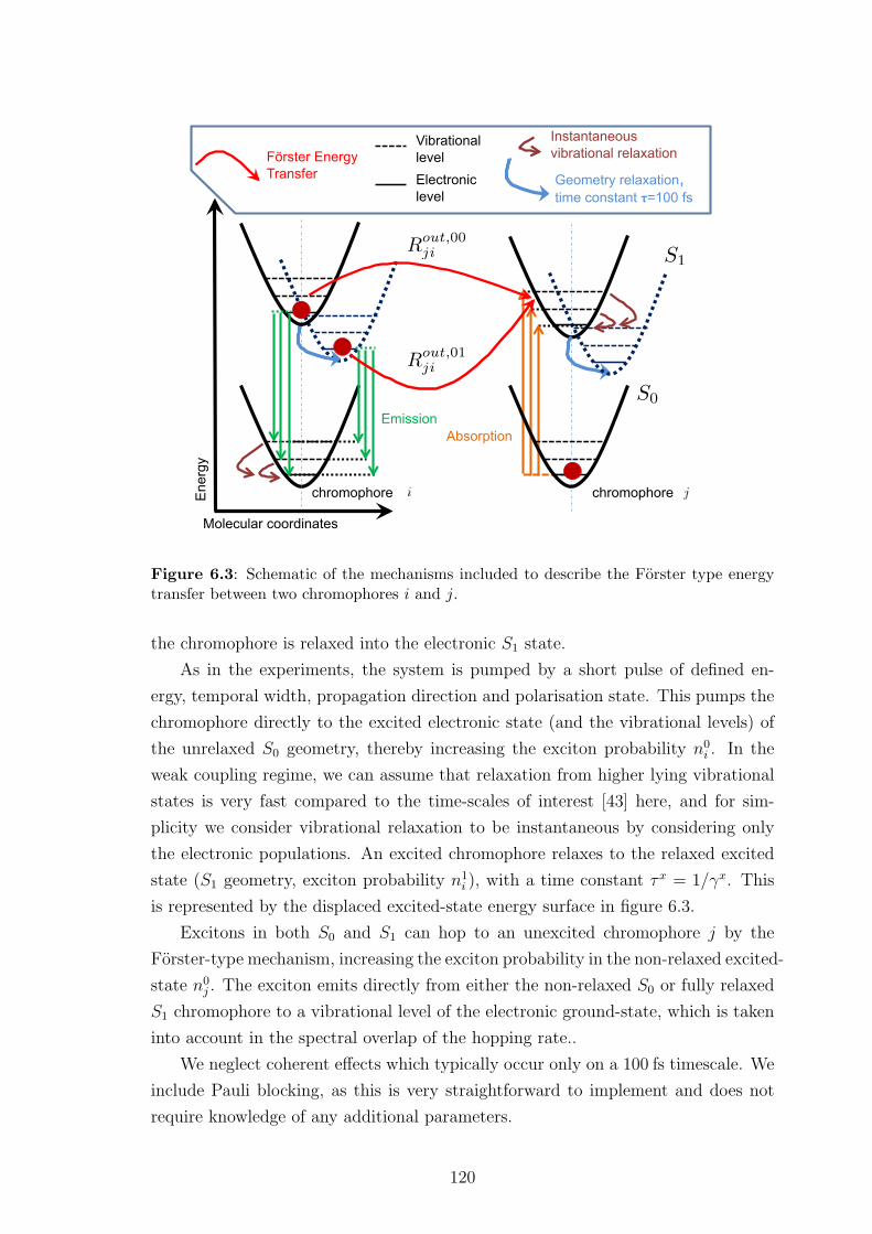
Molecular coordinates

En

erg

y

Emission

Absorption

Instantaneous

vibrational relaxation

Geometry relaxation, time constant τ=100 fs

Förster Energy

Transfer

Vibrational

level

Electronic

level

chromophore chromophore

S0

S1

Rout,01

ji

Rout,00

ji

Figure 6.3: Schematic of the mechanisms included to describe the Forster type energytransfer between two chromophores i and j.

the chromophore is relaxed into the electronic S1 state.

As in the experiments, the system is pumped by a short pulse of defined en-

ergy, temporal width, propagation direction and polarisation state. This pumps the

chromophore directly to the excited electronic state (and the vibrational levels) of

the unrelaxed S0 geometry, thereby increasing the exciton probability n0i . In the

weak coupling regime, we can assume that relaxation from higher lying vibrational

states is very fast compared to the time-scales of interest [43] here, and for sim-

plicity we consider vibrational relaxation to be instantaneous by considering only

the electronic populations. An excited chromophore relaxes to the relaxed excited

state (S1 geometry, exciton probability n1i ), with a time constant τx = 1/γx. This

is represented by the displaced excited-state energy surface in figure 6.3.

Excitons in both S0 and S1 can hop to an unexcited chromophore j by the

Forster-type mechanism, increasing the exciton probability in the non-relaxed excited-

state n0j . The exciton emits directly from either the non-relaxed S0 or fully relaxed

S1 chromophore to a vibrational level of the electronic ground-state, which is taken

into account in the spectral overlap of the hopping rate..

We neglect coherent effects which typically occur only on a 100 fs timescale. We

include Pauli blocking, as this is very straightforward to implement and does not

require knowledge of any additional parameters.

120

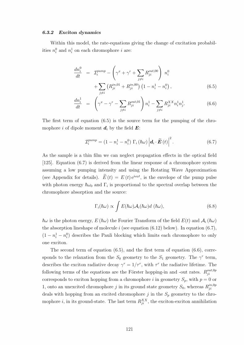
6.3.2 Exciton dynamics

Within this model, the rate-equations giving the change of excitation probabil-

ities n0i and n1

i on each chromophore i are:

dn0i

dt= Ipump

i −(γx + γr +

∑

j 6=i

Rout,00ji

)n0i

+∑

j 6=i

(Rin,01

ji +Rin,00ji

) (1− n1

i − n0i

), (6.5)

dn1i

dt=

(γx − γr −

∑

j 6=i

Rout,01ji

)n1i −

∑

j 6=i

RXXji n1

in1j . (6.6)

The first term of equation (6.5) is the source term for the pumping of the chro-

mophore i of dipole moment di by the field E:

Ipumpi = (1− n1

i − n0i ) Γi (~ω)

∣∣∣di · E (t)∣∣∣2

. (6.7)

As the sample is a thin film we can neglect propagation effects in the optical field

[125]. Equation (6.7) is derived from the linear response of a chromophore system

assuming a low pumping intensity and using the Rotating Wave Approximation

(see Appendix for details). E (t) = E (t) eiω0t, is the envelope of the pump pulse

with photon energy ~ω0 and Γi is proportional to the spectral overlap between the

chromophore absorption and the source:

Γi(~ω) ∝∫

E(~ω)Ai(~ω)d (~ω), (6.8)

~ω is the photon energy, E (~ω) the Fourier Transform of the field E(t) and Ai (~ω)

the absorption lineshape of molecule i (see equation (6.12) below). In equation (6.7),

(1− n1i − n0

i ) describes the Pauli blocking which limits each chromophore to only

one exciton.

The second term of equation (6.5), and the first term of equation (6.6), corre-

sponds to the relaxation from the S0 geometry to the S1 geometry. The γr term,

describes the exciton radiative decay γr = 1/τ r, with τ r the radiative lifetime. The

following terms of the equations are the Forster hopping-in and -out rates. Rout,0pji

corresponds to exciton hopping from a chromophore i in geometry Sp, with p = 0 or

1, onto an unexcited chromophore j in its ground state geometry S0, whereas Rin,0pji

deals with hopping from an excited chromophore j in the Sp geometry to the chro-

mophore i, in its ground-state. The last term RXXji , the exciton-exciton annihilation

121

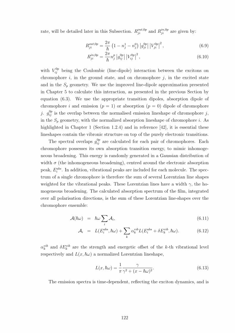
rate, will be detailed later in this Subsection. Rout,0pji and Rin,0p

ji are given by:

Rout,0pji =

2π

~

(1− n1

j − n0j

) ∣∣g0pji∣∣ ∣∣V 0p

ji

∣∣2 , (6.9)

Rin,0pji =

2π

~npj

∣∣g0pij∣∣ ∣∣V 0p

ij

∣∣2 , (6.10)

with V 0pij being the Coulombic (line-dipole) interaction between the excitons on

chromophore i, in the ground state, and on chromophore j, in the excited state

and in the Sp geometry. We use the improved line-dipole approximation presented

in Chapter 5 to calculate this interaction, as presented in the previous Section by

equation (6.3). We use the appropriate transition dipoles, absorption dipole of

chromophore i and emission (p = 1) or absorption (p = 0) dipole of chromophore

j. g0pij is the overlap between the normalised emission lineshape of chromophore j,

in the Sp geometry, with the normalized absorption lineshape of chromophore i. As

highlighted in Chapter 1 (Section 1.2.4) and in reference [42], it is essential these

lineshapes contain the vibronic structure on top of the purely electronic transitions.

The spectral overlaps g0pij are calculated for each pair of chromophores. Each

chromophore possesses its own absorption transition energy, to mimic inhomoge-

neous broadening. This energy is randomly generated in a Gaussian distribution of

width σ (the inhomogeneous broadening), centred around the electronic absorption

peak, Eabsi . In addition, vibrational peaks are included for each molecule. The spec-

trum of a single chromophore is therefore the sum of several Lorentzian line shapes

weighted for the vibrational peaks. These Lorentzian lines have a width γ, the ho-

mogeneous broadening. The calculated absorption spectrum of the film, integrated

over all polarisation directions, is the sum of these Lorentzian line-shapes over the

chromophore ensemble:

A(~ω) = ~ω∑

i

Ai, (6.11)

Ai = L(Eabsi , ~ω) +

∑

k

αvibk L(Eabs

i + δEvibk , ~ω). (6.12)

αvibk and δEvib

k are the strength and energetic offset of the k-th vibrational level

respectively and L(x, ~ω) a normalized Lorentzian lineshape,

L(x, ~ω) =1

π

γ

γ2 + (x− ~ω)2. (6.13)

The emission spectra is time-dependent, reflecting the exciton dynamics, and is

122

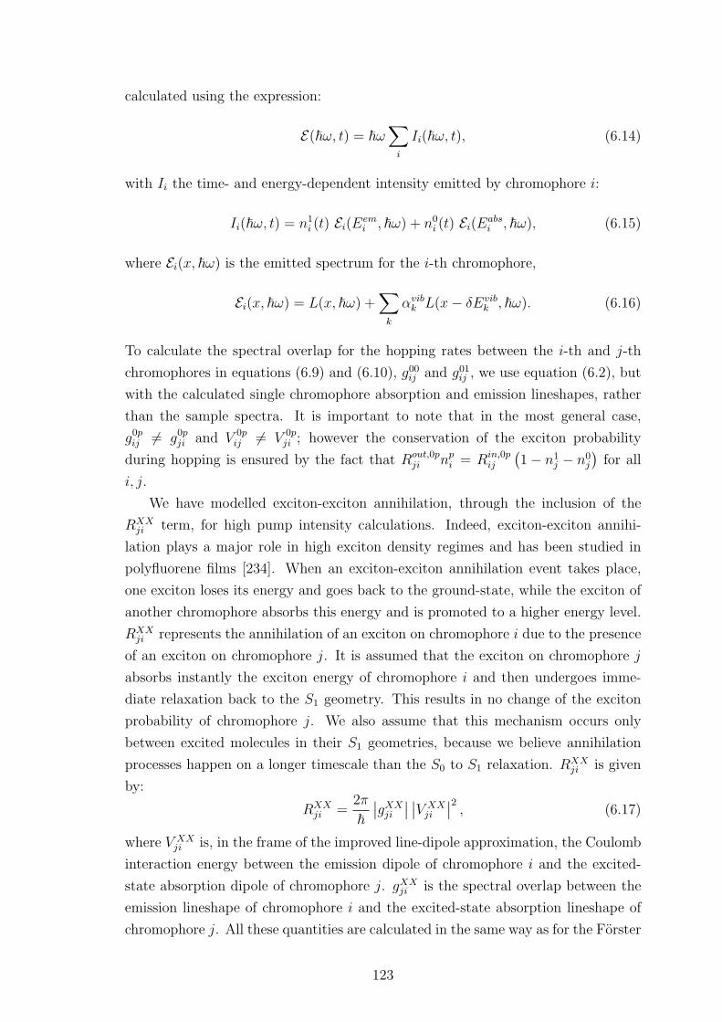
calculated using the expression:

E(~ω, t) = ~ω∑

i

Ii(~ω, t), (6.14)

with Ii the time- and energy-dependent intensity emitted by chromophore i:

Ii(~ω, t) = n1i (t) Ei(Eem

i , ~ω) + n0i (t) Ei(Eabs

i , ~ω), (6.15)

where Ei(x, ~ω) is the emitted spectrum for the i-th chromophore,

Ei(x, ~ω) = L(x, ~ω) +∑

k

αvibk L(x− δEvib

k , ~ω). (6.16)

To calculate the spectral overlap for the hopping rates between the i-th and j-th

chromophores in equations (6.9) and (6.10), g00ij and g01ij , we use equation (6.2), but

with the calculated single chromophore absorption and emission lineshapes, rather

than the sample spectra. It is important to note that in the most general case,

g0pij 6= g0pji and V 0pij 6= V 0p

ji ; however the conservation of the exciton probability

during hopping is ensured by the fact that Rout,0pji np

i = Rin,0pij

(1− n1

j − n0j

)for all

i, j.

We have modelled exciton-exciton annihilation, through the inclusion of the

RXXji term, for high pump intensity calculations. Indeed, exciton-exciton annihi-

lation plays a major role in high exciton density regimes and has been studied in

polyfluorene films [234]. When an exciton-exciton annihilation event takes place,

one exciton loses its energy and goes back to the ground-state, while the exciton of

another chromophore absorbs this energy and is promoted to a higher energy level.

RXXji represents the annihilation of an exciton on chromophore i due to the presence

of an exciton on chromophore j. It is assumed that the exciton on chromophore j

absorbs instantly the exciton energy of chromophore i and then undergoes imme-

diate relaxation back to the S1 geometry. This results in no change of the exciton

probability of chromophore j. We also assume that this mechanism occurs only

between excited molecules in their S1 geometries, because we believe annihilation

processes happen on a longer timescale than the S0 to S1 relaxation. RXXji is given

by:

RXXji =

2π

~

∣∣gXXji

∣∣ ∣∣V XXji

∣∣2 , (6.17)

where V XXji is, in the frame of the improved line-dipole approximation, the Coulomb

interaction energy between the emission dipole of chromophore i and the excited-

state absorption dipole of chromophore j. gXXji is the spectral overlap between the

emission lineshape of chromophore i and the excited-state absorption lineshape of

chromophore j. All these quantities are calculated in the same way as for the Forster

123

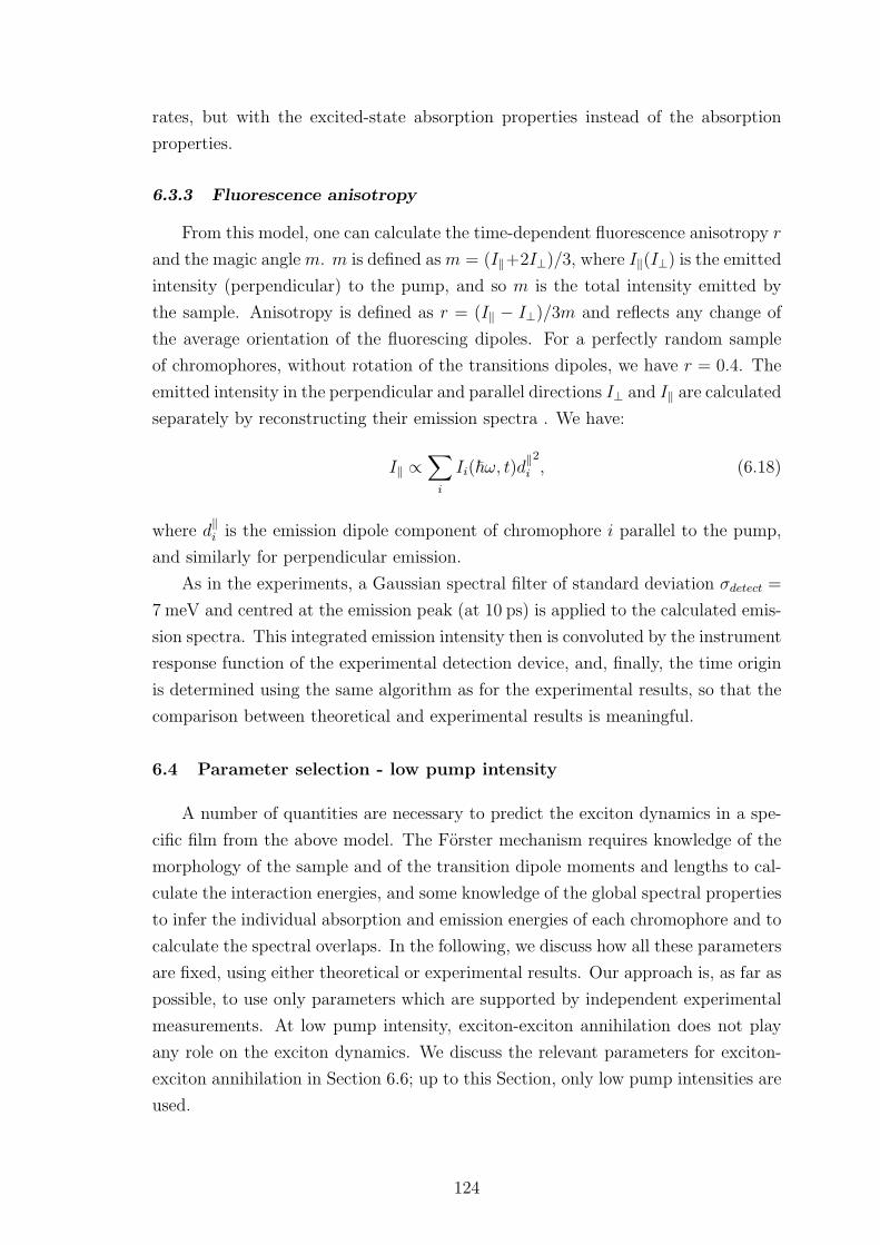
rates, but with the excited-state absorption properties instead of the absorption

properties.

6.3.3 Fluorescence anisotropy

From this model, one can calculate the time-dependent fluorescence anisotropy r

and the magic anglem. m is defined asm = (I‖+2I⊥)/3, where I‖(I⊥) is the emitted

intensity (perpendicular) to the pump, and so m is the total intensity emitted by

the sample. Anisotropy is defined as r = (I‖ − I⊥)/3m and reflects any change of

the average orientation of the fluorescing dipoles. For a perfectly random sample

of chromophores, without rotation of the transitions dipoles, we have r = 0.4. The

emitted intensity in the perpendicular and parallel directions I⊥ and I‖ are calculated

separately by reconstructing their emission spectra . We have:

I‖ ∝∑

i

Ii(~ω, t)d‖i

2, (6.18)

where d‖i is the emission dipole component of chromophore i parallel to the pump,

and similarly for perpendicular emission.

As in the experiments, a Gaussian spectral filter of standard deviation σdetect =

7 meV and centred at the emission peak (at 10 ps) is applied to the calculated emis-

sion spectra. This integrated emission intensity then is convoluted by the instrument

response function of the experimental detection device, and, finally, the time origin

is determined using the same algorithm as for the experimental results, so that the

comparison between theoretical and experimental results is meaningful.

6.4 Parameter selection - low pump intensity

A number of quantities are necessary to predict the exciton dynamics in a spe-

cific film from the above model. The Forster mechanism requires knowledge of the

morphology of the sample and of the transition dipole moments and lengths to cal-

culate the interaction energies, and some knowledge of the global spectral properties

to infer the individual absorption and emission energies of each chromophore and to

calculate the spectral overlaps. In the following, we discuss how all these parameters

are fixed, using either theoretical or experimental results. Our approach is, as far as

possible, to use only parameters which are supported by independent experimental

measurements. At low pump intensity, exciton-exciton annihilation does not play

any role on the exciton dynamics. We discuss the relevant parameters for exciton-

exciton annihilation in Section 6.6; up to this Section, only low pump intensities are

used.

124

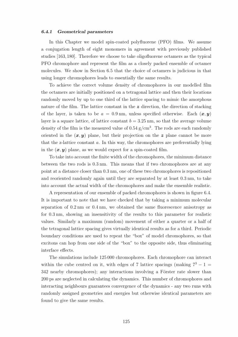
6.4.1 Geometrical parameters

In this Chapter we model spin-coated polyfluorene (PFO) films. We assume

a conjugation length of eight monomers in agreement with previously published

studies [163,180]. Therefore we choose to take oligofluorene octamers as the typical

PFO chromophore and represent the film as a closely packed ensemble of octamer

molecules. We show in Section 6.5 that the choice of octamers is judicious in that

using longer chromophores leads to essentially the same results.

To achieve the correct volume density of chromophores in our modelled film

the octamers are initially positioned on a tetragonal lattice and then their locations

randomly moved by up to one third of the lattice spacing to mimic the amorphous

nature of the film. The lattice constant in the z direction, the direction of stacking

of the layer, is taken to be a = 0.9 nm, unless specified otherwise. Each (x,y)

layer is a square lattice, of lattice constant b = 3.25 nm, so that the average volume

density of the film is the measured value of 0.54 g/cm3. The rods are each randomly

oriented in the (x,y) plane, but their projection on the z plane cannot be more

that the z-lattice constant a. In this way, the chromophores are preferentially lying

in the (x,y) plane, as we would expect for a spin-coated film.

To take into account the finite width of the chromophores, the minimum distance

between the two rods is 0.3 nm. This means that if two chromophores are at any

point at a distance closer than 0.3 nm, one of these two chromophores is repositioned

and reoriented randomly again until they are separated by at least 0.3 nm, to take

into account the actual width of the chromophores and make the ensemble realistic.

A representation of our ensemble of packed chromophores is shown in figure 6.4.

It is important to note that we have checked that by taking a minimum molecular

separation of 0.2 nm or 0.4 nm, we obtained the same fluorescence anisotropy as

for 0.3 nm, showing an insensitivity of the results to this parameter for realistic

values. Similarly a maximum (random) movement of either a quarter or a half of

the tetragonal lattice spacing gives virtually identical results as for a third. Periodic

boundary conditions are used to repeat the “box” of model chromophores, so that

excitons can hop from one side of the “box” to the opposite side, thus eliminating

interface effects.

The simulations include 125 000 chromophores. Each chromophore can interact

within the cube centred on it, with edges of 7 lattice spacings (making 73 − 1 =

342 nearby chromophores); any interactions involving a Forster rate slower than

200 ps are neglected in calculating the dynamics. This number of chromophores and

interacting neighbours guarantees convergence of the dynamics - any two runs with

randomly assigned geometries and energies but otherwise identical parameters are

found to give the same results.

125

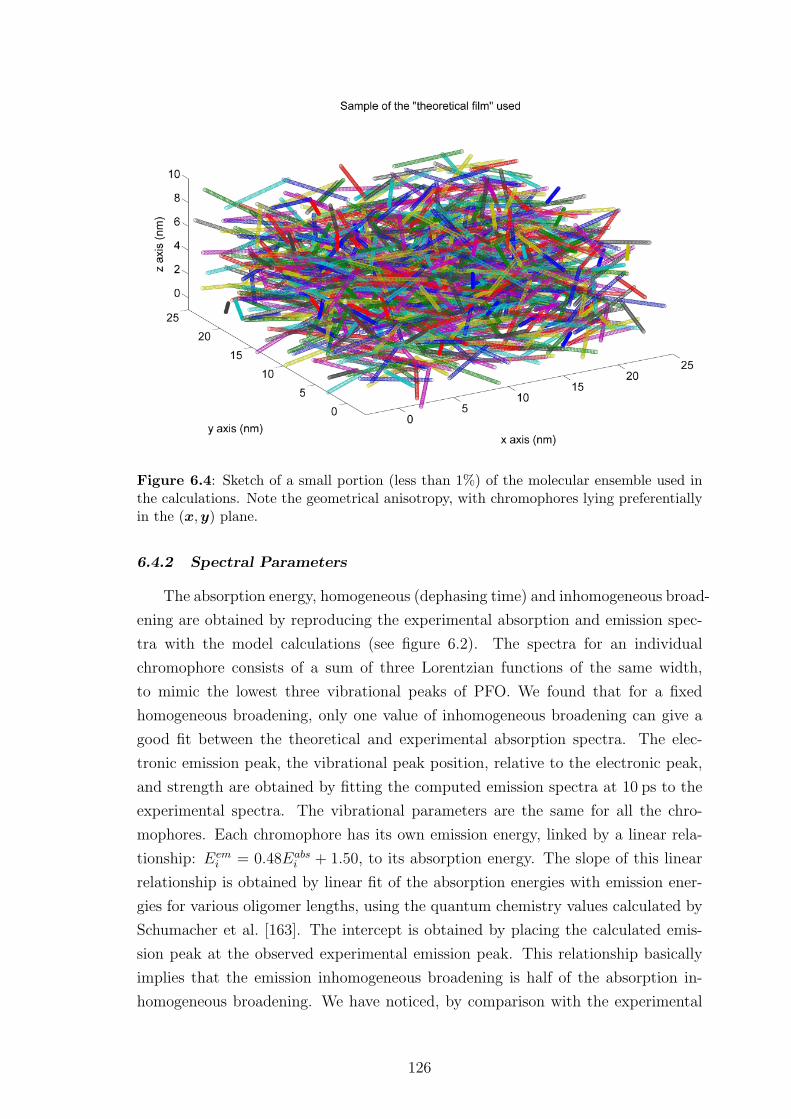
Figure 6.4: Sketch of a small portion (less than 1%) of the molecular ensemble used inthe calculations. Note the geometrical anisotropy, with chromophores lying preferentiallyin the (x,y) plane.

6.4.2 Spectral Parameters

The absorption energy, homogeneous (dephasing time) and inhomogeneous broad-

ening are obtained by reproducing the experimental absorption and emission spec-

tra with the model calculations (see figure 6.2). The spectra for an individual

chromophore consists of a sum of three Lorentzian functions of the same width,

to mimic the lowest three vibrational peaks of PFO. We found that for a fixed

homogeneous broadening, only one value of inhomogeneous broadening can give a

good fit between the theoretical and experimental absorption spectra. The elec-

tronic emission peak, the vibrational peak position, relative to the electronic peak,

and strength are obtained by fitting the computed emission spectra at 10 ps to the

experimental spectra. The vibrational parameters are the same for all the chro-

mophores. Each chromophore has its own emission energy, linked by a linear rela-

tionship: Eemi = 0.48Eabs

i + 1.50, to its absorption energy. The slope of this linear

relationship is obtained by linear fit of the absorption energies with emission ener-

gies for various oligomer lengths, using the quantum chemistry values calculated by

Schumacher et al. [163]. The intercept is obtained by placing the calculated emis-

sion peak at the observed experimental emission peak. This relationship basically

implies that the emission inhomogeneous broadening is half of the absorption in-

homogeneous broadening. We have noticed, by comparison with the experimental

126

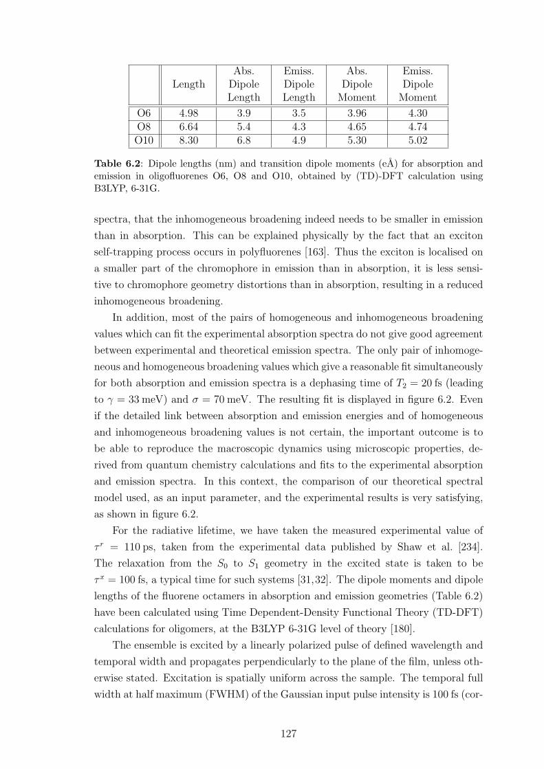
LengthAbs.DipoleLength

Emiss.DipoleLength

Abs.DipoleMoment

Emiss.DipoleMoment

O6 4.98 3.9 3.5 3.96 4.30O8 6.64 5.4 4.3 4.65 4.74O10 8.30 6.8 4.9 5.30 5.02

Table 6.2: Dipole lengths (nm) and transition dipole moments (eA) for absorption andemission in oligofluorenes O6, O8 and O10, obtained by (TD)-DFT calculation usingB3LYP, 6-31G.

spectra, that the inhomogeneous broadening indeed needs to be smaller in emission

than in absorption. This can be explained physically by the fact that an exciton

self-trapping process occurs in polyfluorenes [163]. Thus the exciton is localised on

a smaller part of the chromophore in emission than in absorption, it is less sensi-

tive to chromophore geometry distortions than in absorption, resulting in a reduced

inhomogeneous broadening.

In addition, most of the pairs of homogeneous and inhomogeneous broadening

values which can fit the experimental absorption spectra do not give good agreement

between experimental and theoretical emission spectra. The only pair of inhomoge-

neous and homogeneous broadening values which give a reasonable fit simultaneously

for both absorption and emission spectra is a dephasing time of T2 = 20 fs (leading

to γ = 33 meV) and σ = 70 meV. The resulting fit is displayed in figure 6.2. Even

if the detailed link between absorption and emission energies and of homogeneous

and inhomogeneous broadening values is not certain, the important outcome is to

be able to reproduce the macroscopic dynamics using microscopic properties, de-

rived from quantum chemistry calculations and fits to the experimental absorption

and emission spectra. In this context, the comparison of our theoretical spectral

model used, as an input parameter, and the experimental results is very satisfying,

as shown in figure 6.2.

For the radiative lifetime, we have taken the measured experimental value of

τ r = 110 ps, taken from the experimental data published by Shaw et al. [234].

The relaxation from the S0 to S1 geometry in the excited state is taken to be

τx = 100 fs, a typical time for such systems [31,32]. The dipole moments and dipole

lengths of the fluorene octamers in absorption and emission geometries (Table 6.2)

have been calculated using Time Dependent-Density Functional Theory (TD-DFT)

calculations for oligomers, at the B3LYP 6-31G level of theory [180].

The ensemble is excited by a linearly polarized pulse of defined wavelength and

temporal width and propagates perpendicularly to the plane of the film, unless oth-

erwise stated. Excitation is spatially uniform across the sample. The temporal full

width at half maximum (FWHM) of the Gaussian input pulse intensity is 100 fs (cor-

127

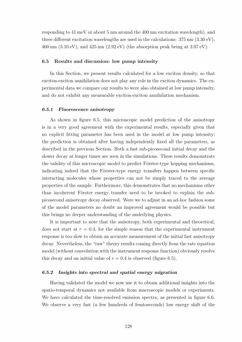
responding to 41 meV or about 5 nm around the 400 nm excitation wavelength), and

three different excitation wavelengths are used in the calculations: 375 nm (3.30 eV),

400 nm (3.10 eV), and 425 nm (2.92 eV) (the absorption peak being at 3.07 eV).

6.5 Results and discussion: low pump intensity

In this Section, we present results calculated for a low exciton density, so that

exciton-exciton annihilation does not play any role in the exciton dynamics. The ex-

perimental data we compare our results to were also obtained at low pump intensity,

and do not exhibit any measurable exciton-exciton annihilation mechanism.

6.5.1 Fluorescence anisotropy

As shown in figure 6.5, this microscopic model prediction of the anisotropy

is in a very good agreement with the experimental results, especially given that

no explicit fitting parameter has been used in the model at low pump intensity;

the prediction is obtained after having independently fixed all the parameters, as

described in the previous Section. Both a fast sub-picosecond initial decay and the

slower decay at longer times are seen in the simulations. These results demonstrate

the validity of this microscopic model to predict Forster-type hopping mechanisms,

indicating indeed that the Forster-type energy transfers happen between specific

interacting molecules whose properties can not be simply traced to the average

properties of the sample. Furthermore, this demonstrates that no mechanisms other

than incoherent Forster energy transfer need to be invoked to explain the sub-

picosecond anisotropy decay observed. Were we to adjust in an ad-hoc fashion some

of the model parameters no doubt an improved agreement would be possible but

this brings no deeper understanding of the underlying physics.

It is important to note that the anisotropy, both experimental and theoretical,

does not start at r = 0.4, for the simple reason that the experimental instrument

response is too slow to obtain an accurate measurement of the initial fast anisotropy

decay. Nevertheless, the “raw” theory results coming directly from the rate equation

model (without convolution with the instrument response function) obviously resolve

this decay and an initial value of r = 0.4 is observed (figure 6.5).

6.5.2 Insights into spectral and spatial energy migration

Having validated the model we now use it to obtain additional insights into the

spatio-temporal dynamics not available from macroscopic models or experiments.

We have calculated the time-resolved emission spectra, as presented in figure 6.6.

We observe a very fast (a few hundreds of femtoseconds) low energy shift of the

128

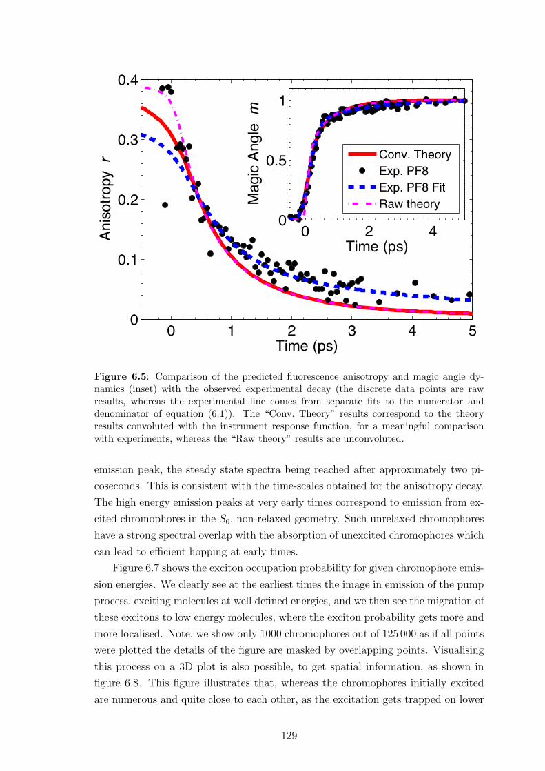
0 1 2 3 4 50

0.1

0.2

0.3

0.4

Time (ps)

An

iso

tro

py r

0 2 40

0.5

1

Time (ps)M

ag

ic A

ng

le m

Conv. Theory

Exp. PF8

Exp. PF8 Fit

Raw theory

Figure 6.5: Comparison of the predicted fluorescence anisotropy and magic angle dy-namics (inset) with the observed experimental decay (the discrete data points are rawresults, whereas the experimental line comes from separate fits to the numerator anddenominator of equation (6.1)). The “Conv. Theory” results correspond to the theoryresults convoluted with the instrument response function, for a meaningful comparisonwith experiments, whereas the “Raw theory” results are unconvoluted.

emission peak, the steady state spectra being reached after approximately two pi-

coseconds. This is consistent with the time-scales obtained for the anisotropy decay.

The high energy emission peaks at very early times correspond to emission from ex-

cited chromophores in the S0, non-relaxed geometry. Such unrelaxed chromophores

have a strong spectral overlap with the absorption of unexcited chromophores which

can lead to efficient hopping at early times.

Figure 6.7 shows the exciton occupation probability for given chromophore emis-

sion energies. We clearly see at the earliest times the image in emission of the pump

process, exciting molecules at well defined energies, and we then see the migration of

these excitons to low energy molecules, where the exciton probability gets more and

more localised. Note, we show only 1000 chromophores out of 125 000 as if all points

were plotted the details of the figure are masked by overlapping points. Visualising

this process on a 3D plot is also possible, to get spatial information, as shown in

figure 6.8. This figure illustrates that, whereas the chromophores initially excited

are numerous and quite close to each other, as the excitation gets trapped on lower

129

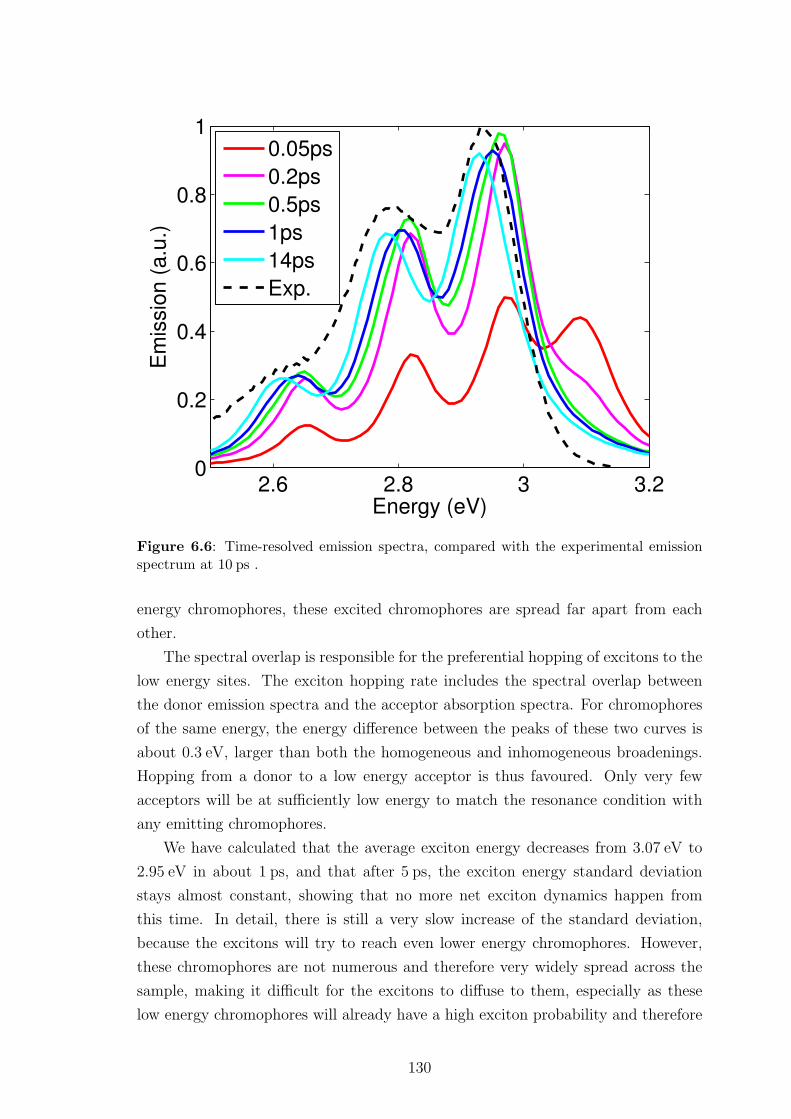
2.6 2.8 3 3.20

0.2

0.4

0.6

0.8

1

Energy (eV)

Em

issio

n (

a.u

.)

0.05ps

0.2ps

0.5ps

1ps

14ps

Exp.

Figure 6.6: Time-resolved emission spectra, compared with the experimental emissionspectrum at 10 ps .

energy chromophores, these excited chromophores are spread far apart from each

other.

The spectral overlap is responsible for the preferential hopping of excitons to the

low energy sites. The exciton hopping rate includes the spectral overlap between

the donor emission spectra and the acceptor absorption spectra. For chromophores

of the same energy, the energy difference between the peaks of these two curves is

about 0.3 eV, larger than both the homogeneous and inhomogeneous broadenings.

Hopping from a donor to a low energy acceptor is thus favoured. Only very few

acceptors will be at sufficiently low energy to match the resonance condition with

any emitting chromophores.

We have calculated that the average exciton energy decreases from 3.07 eV to

2.95 eV in about 1 ps, and that after 5 ps, the exciton energy standard deviation

stays almost constant, showing that no more net exciton dynamics happen from

this time. In detail, there is still a very slow increase of the standard deviation,

because the excitons will try to reach even lower energy chromophores. However,

these chromophores are not numerous and therefore very widely spread across the

sample, making it difficult for the excitons to diffuse to them, especially as these

low energy chromophores will already have a high exciton probability and therefore

130

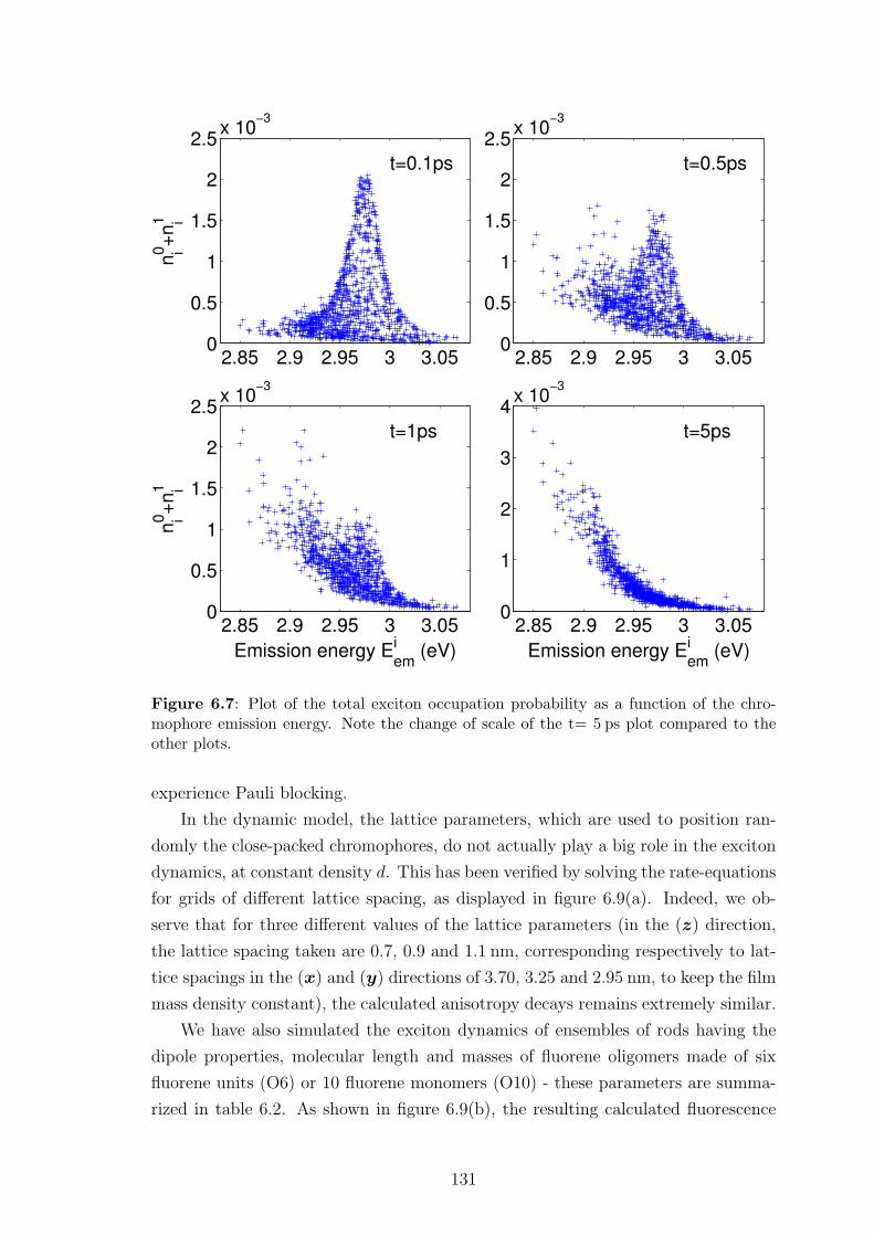
2.85 2.9 2.95 3 3.050

0.5

1

1.5

2

2.5x 10

−3

ni0+

ni1

t=0.1ps

2.85 2.9 2.95 3 3.050

0.5

1

1.5

2

2.5x 10

−3

t=0.5ps

2.85 2.9 2.95 3 3.050

0.5

1

1.5

2

2.5x 10

−3

Emission energy Eem

i (eV)

ni0+

ni1

t=1ps

2.85 2.9 2.95 3 3.050

1

2

3

4x 10

−3

Emission energy Eem

i (eV)

t=5ps

Figure 6.7: Plot of the total exciton occupation probability as a function of the chro-mophore emission energy. Note the change of scale of the t= 5 ps plot compared to theother plots.

experience Pauli blocking.

In the dynamic model, the lattice parameters, which are used to position ran-

domly the close-packed chromophores, do not actually play a big role in the exciton

dynamics, at constant density d. This has been verified by solving the rate-equations

for grids of different lattice spacing, as displayed in figure 6.9(a). Indeed, we ob-

serve that for three different values of the lattice parameters (in the (z) direction,

the lattice spacing taken are 0.7, 0.9 and 1.1 nm, corresponding respectively to lat-

tice spacings in the (x) and (y) directions of 3.70, 3.25 and 2.95 nm, to keep the film

mass density constant), the calculated anisotropy decays remains extremely similar.

We have also simulated the exciton dynamics of ensembles of rods having the

dipole properties, molecular length and masses of fluorene oligomers made of six

fluorene units (O6) or 10 fluorene monomers (O10) - these parameters are summa-

rized in table 6.2. As shown in figure 6.9(b), the resulting calculated fluorescence

131

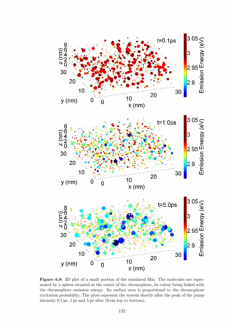
Figure 6.8: 3D plot of a small portion of the simulated film. The molecules are repre-sented by a sphere situated at the centre of the chromophore, its colour being linked withthe chromophore emission energy. Its surface area is proportional to the chromophoreexcitation probability. The plots represent the system shortly after the peak of the pumpintensity 0.1 ps, 1 ps and 5 ps after (from top to bottom).

132

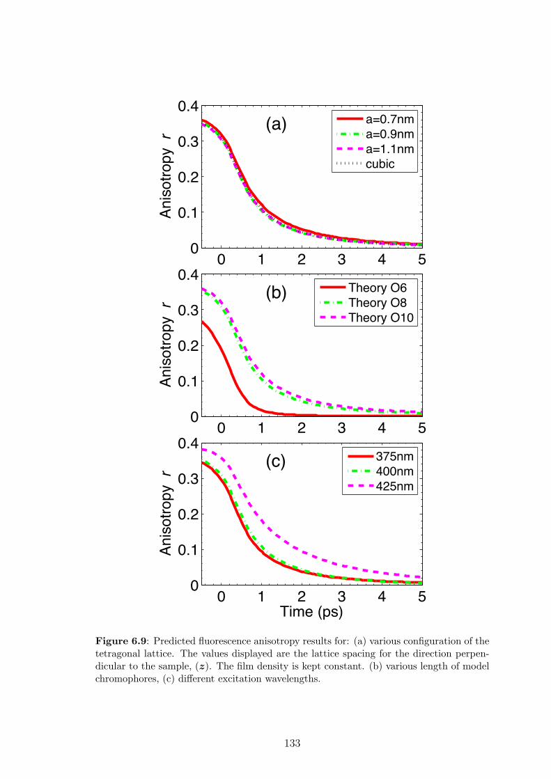
0 1 2 3 4 50

0.1

0.2

0.3

0.4

An

iso

tro

py r

(a) a=0.7nm

a=0.9nm

a=1.1nm

cubic

0 1 2 3 4 50

0.1

0.2

0.3

0.4

An

iso

tro

py r

(b) Theory O6

Theory O8

Theory O10

0 1 2 3 4 50

0.1

0.2

0.3

0.4

Time (ps)

An

iso

tro

py r

(c) 375nm

400nm

425nm

Figure 6.9: Predicted fluorescence anisotropy results for: (a) various configuration of thetetragonal lattice. The values displayed are the lattice spacing for the direction perpen-dicular to the sample, (z). The film density is kept constant. (b) various length of modelchromophores, (c) different excitation wavelengths.

133

anisotropy for O6 chromophores is faster than for O8, because the molecular interac-

tions are stronger for smaller length oligomers (at fixed transition dipole moment),

which are also more closely packed. However, the results are identical for O8 and

O10, giving further support that these lengths are typical conjugation lengths for

polyfluorene molecules.

Having a successful microscopic model for exciton diffusion enables us to gain

deeper knowledge of these diffusion mechanisms. It is possible to analyse the Forster-

type interaction rates involved in the model to deduce the number and the strength

of these interactions, and which chromophores are primarily involved. For instance,

the middle plot of figure 6.10 shows, for the same parameters as above, a histogram

of the time-constants associated with the out-scattering (Rout,0pji ) rates, where the

term (1− n1i − n0

i ) is assumed to be unity at these low probabilities. We observe that

about 6% of chromophores possess an interaction term Rout,01ji with another chro-

mophore faster than 1 ps, and 16% between 1 and 2 ps, so that more than a fifth

of the molecules have at least one neighbour for which the interaction is faster than

2 ps, explaining the fast anisotropy decay observed. In addition, the average absorp-

tion energies and the centre-to-centre separations of the chromophores as a function

of their Forster interaction time is also displayed in figure 6.10. The fastest interac-

tions correspond to chromophores with the largest energy difference, consistent with

the spectral overlap argument given above. This shows that we should indeed ex-

pect the fast exciton diffusion processes to be over after a few picoseconds, and that

most excitons directly go to the low energy sites, without going through molecules

of intermediate energies. Additionally, with our excitation energy at 3.10 eV, we ini-

tially excite the interacting pairs with the fastest Forster hopping rates, explaining

the fast depolarisation we observe. As expected, the centre-to-centre separation of

the chromophore pairs increases with their Forster transfer times. It is important to

note that the centre-to-centre chromophore separations of the fastest Forster rates

are relatively large, above 3 nm, significantly larger than the average chromophore

separation in the plane (0.9 nm). Therefore, the fastest Forster exciton transfers do

not necessarily happen between an excited chromophore and its nearest neighbour,

but between an excited chromophore and a spectrally matched lower energy chro-

mophore. This explains the insensitivity of the exciton dynamics of the geometric

parameters used for the generation of the ensemble of model chromophores. Indeed,

rather than the distance of the closest neighbours, the spatial parameter of impor-

tance is the film density, as the chromophores interact with a range of chromophores

situated further than the closest neighbour, and therefore a lot more chromophores

(as the number of chromophores situated at a certain radius increases with the ra-

dius squared). This is further illustrated by the top and bottom plots of figure 6.10,

where the homogeneous broadening has been changed to either σ = 30 meV (top)

134

or σ = 110 meV (bottom). In the case of σ = 30 meV, the chromophore energies

are almost all the same for interactions slower than 5 ps. What makes the interac-

tions slower is then the increase of the centre-to-centre separation. In the case of

σ = 110 meV, there are many more pairs of very different energies, resulting in a

much greater number of interacting pairs faster than 5 ps. We can also remark that

the Rout,00ji hops are slower than the Rout,01

ji hops. This is perhaps counter-intuitive,

as the spectral overlap will be larger for the case where the donor emits at the

absorption energy, but can be explained by the weaker absorption dipole moment,

compared to the emission dipole.

Additionally, the microscopic rate-equation model enables the choice of different

excitation wavelengths and effectively simulates the effect on the system. We would

expect the exciton dynamics to be modified if the pump has an energy above or

below the main absorption peak. Indeed, if the pump has a lower energy than

the absorption peak, then the chromophores excited by the pump will already be

the low energy ones, and thus no spectral diffusion will take place, whereas the

opposite is expected if the pump excites the sample at much higher energy than the

absorption peak. This is successfully predicted by our microscopic “rate-equation”

model, as displayed in figure 6.9(c). The wavelengths we have chosen are 375 nm

(3.30 eV), 400 nm (3.10 eV), and 425 nm (2.92 eV), compared to the absorption peak

at 3.07 eV.

6.5.3 Exciton diffusion length

At low exciton density, when exciton-exciton annihilation effects are negligible,

we are able to obtain diffusion properties from our model. Indeed, excitation of the

ensemble of chromophores by a spatially Gaussian-shaped (rather than uniform)

pump and recording its standard deviation over time will provide knowledge of

the diffusion coefficient and of the diffusion length. When specified, we use such

a technique to obtain the diffusion properties of the sample. An example of the

excitation of the system by a Gaussian-shaped pump is provided in figure 6.11. The

Gaussian is one dimensional, along the x-axis (arbitrarily situated in the plane of

the thin-film), and the plot of figure 6.11 shows the total exciton probability for

all the chromophores situated in the vicinity of one of the 50 grid points along the

x-axis.

The standard one dimensional diffusion equation is [257]:

∂n

∂t= D

∂2n

∂x. (6.19)

By recording the standard deviation of the one dimensional exciton probability,

σD, we obtain the diffusion coefficient D from the solution of this standard one-

135

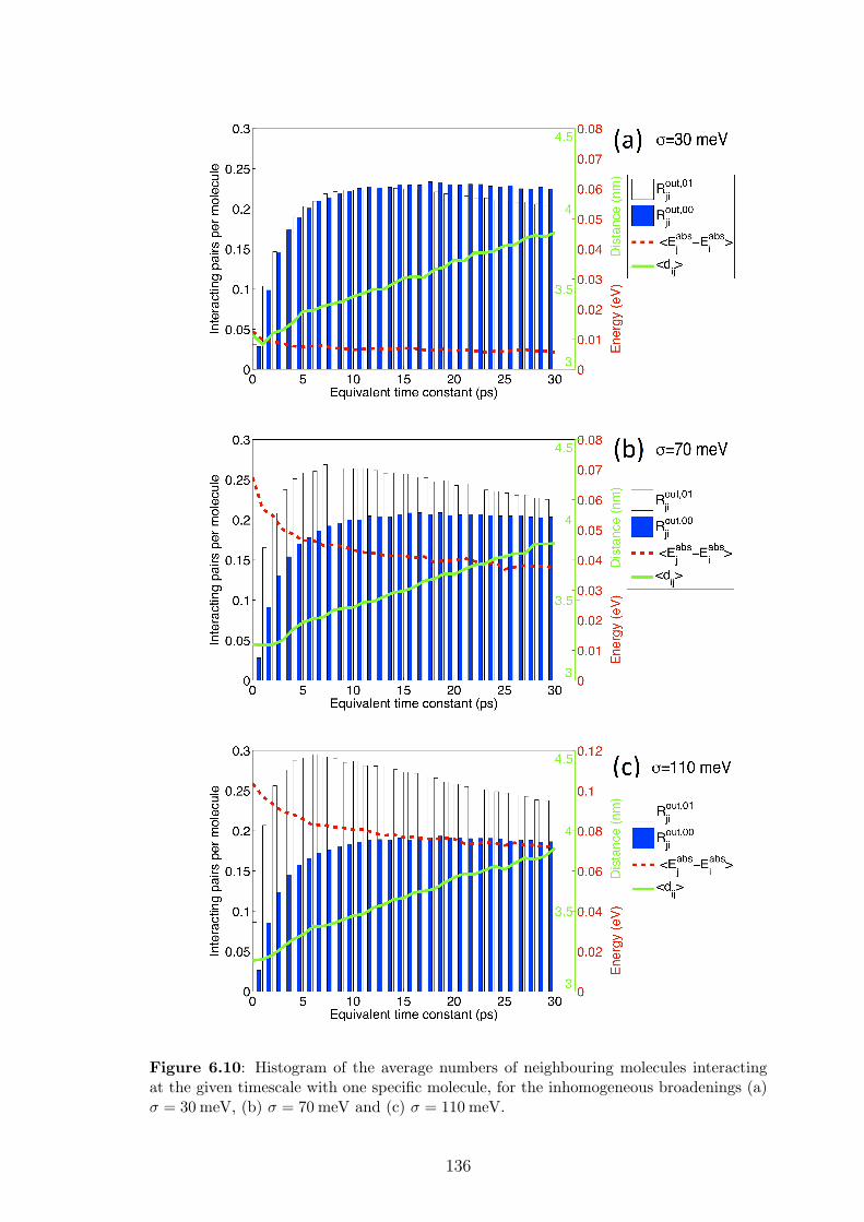
Figure 6.10: Histogram of the average numbers of neighbouring molecules interactingat the given timescale with one specific molecule, for the inhomogeneous broadenings (a)σ = 30 meV, (b) σ = 70 meV and (c) σ = 110 meV.

136

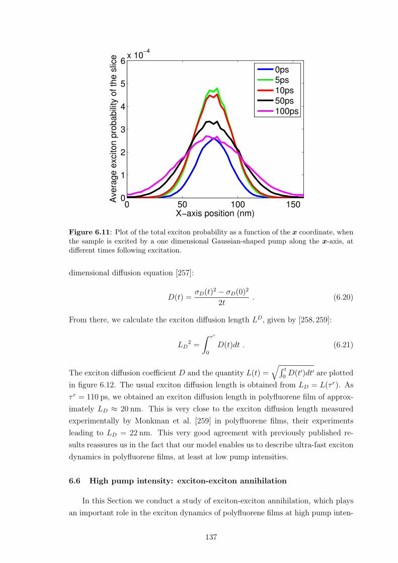
0 50 100 1500

1

2

3

4

5

6x 10

−4

X−axis position (nm)

Ave

rag

e e

xcito

n p

rob

ab

ility

of

the

slic

e

0ps

5ps

10ps

50ps

100ps

Figure 6.11: Plot of the total exciton probability as a function of the x coordinate, whenthe sample is excited by a one dimensional Gaussian-shaped pump along the x-axis, atdifferent times following excitation.

dimensional diffusion equation [257]:

D(t) =σD(t)

2 − σD(0)2

2t. (6.20)

From there, we calculate the exciton diffusion length LD, given by [258,259]:

LD2 =

∫ τr

0

D(t)dt . (6.21)

The exciton diffusion coefficient D and the quantity L(t) =√∫ t

0D(t′)dt′ are plotted

in figure 6.12. The usual exciton diffusion length is obtained from LD = L(τ r). As

τ r = 110 ps, we obtained an exciton diffusion length in polyfluorene film of approx-

imately LD ≈ 20 nm. This is very close to the exciton diffusion length measured

experimentally by Monkman et al. [259] in polyfluorene films, their experiments

leading to LD = 22 nm. This very good agreement with previously published re-

sults reassures us in the fact that our model enables us to describe ultra-fast exciton

dynamics in polyfluorene films, at least at low pump intensities.

6.6 High pump intensity: exciton-exciton annihilation

In this Section we conduct a study of exciton-exciton annihilation, which plays

an important role in the exciton dynamics of polyfluorene films at high pump inten-

137

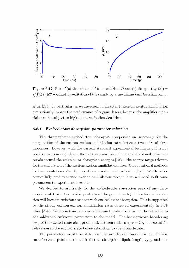
0 10 20 30 40 501

2

3

4

5

Time (ps)

Diffu

sio

n c

oe

ffic

ien

t D

(n

m2/p

s)

(a)

0 20 40 60 80 1000

5

10

15

20

Time (ps)

L(t

) (n

m)

(b)

Figure 6.12: Plot of (a) the exciton diffusion coefficient D and (b) the quantity L(t) =√∫ t0 D(t′)dt′ obtained by excitation of the sample by a one dimensional Gaussian pump.

sities [234]. In particular, as we have seen in Chapter 1, exciton-exciton annihilation

can seriously impact the performance of organic lasers, because the amplifier mate-

rials can be subject to high photo-excitation densities.

6.6.1 Excited-state absorption parameter selection

The chromophores excited-state absorption properties are necessary for the

computation of the exciton-exciton annihilation rates between two pairs of chro-

mophores. However, with the current standard experimental techniques, it is not

possible to accurately obtain the excited-absorption characteristics of molecular ma-

terials around the emission or absorption energies [123] - the energy range relevant

for the calculation of the exciton-exciton annihilation rates. Computational methods

for the calculations of such properties are not reliable yet either [123]. We therefore

cannot fully predict exciton-exciton annihilation rates, but we will need to fit some

parameters to experimental results.

We decided to arbitrarily fix the excited-state absorption peak of any chro-

mophore at twice its emission peak (from the ground state). Therefore an excita-

tion will have its emission resonant with excited-state absorption. This is supported

by the strong exciton-exciton annihilation rates observed experimentally in PF8

films [234]. We do not include any vibrational peaks, because we do not want to

add additional unknown parameters to the model. The homogeneous broadening

γXX of the excited-state absorption peak is taken such as γXX = 2γ, to account for

relaxation to the excited state before relaxation to the ground-state.

The parameters we still need to compute are the exciton-exciton annihilation

rates between pairs are the excited-state absorption dipole length, lXX , and mo-

138

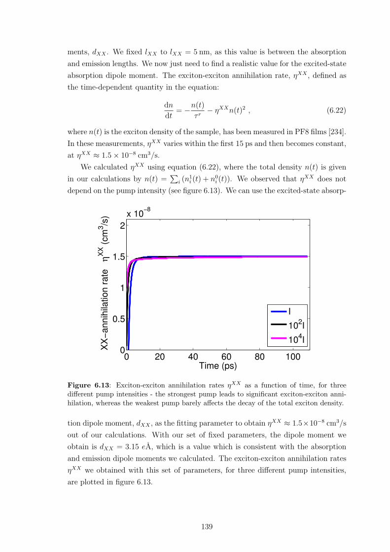
ments, dXX . We fixed lXX to lXX = 5 nm, as this value is between the absorption

and emission lengths. We now just need to find a realistic value for the excited-state

absorption dipole moment. The exciton-exciton annihilation rate, ηXX , defined as

the time-dependent quantity in the equation:

dn

dt= −n(t)

τ r− ηXXn(t)2 , (6.22)

where n(t) is the exciton density of the sample, has been measured in PF8 films [234].

In these measurements, ηXX varies within the first 15 ps and then becomes constant,

at ηXX ≈ 1.5× 10−8 cm3/s.

We calculated ηXX using equation (6.22), where the total density n(t) is given

in our calculations by n(t) =∑

i (n1i (t) + n0

i (t)). We observed that ηXX does not

depend on the pump intensity (see figure 6.13). We can use the excited-state absorp-

0 20 40 60 80 1000

0.5

1

1.5

2

x 10−8

Time (ps)

XX

−a

nn

ihila

tio

n r

ate

η

XX (

cm

3/s

)

I

102I

104I

Figure 6.13: Exciton-exciton annihilation rates ηXX as a function of time, for threedifferent pump intensities - the strongest pump leads to significant exciton-exciton anni-hilation, whereas the weakest pump barely affects the decay of the total exciton density.

tion dipole moment, dXX , as the fitting parameter to obtain ηXX ≈ 1.5×10−8 cm3/s

out of our calculations. With our set of fixed parameters, the dipole moment we

obtain is dXX = 3.15 eA, which is a value which is consistent with the absorption

and emission dipole moments we calculated. The exciton-exciton annihilation rates

ηXX we obtained with this set of parameters, for three different pump intensities,

are plotted in figure 6.13.

139

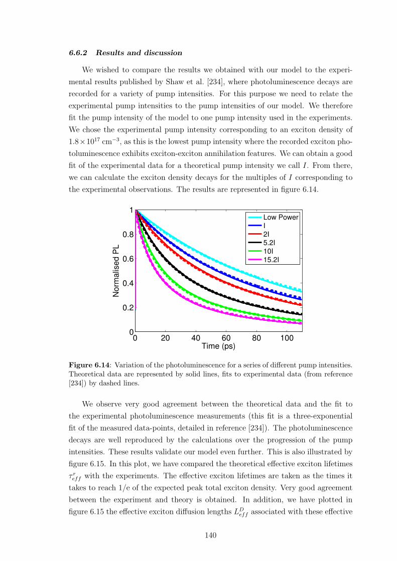
6.6.2 Results and discussion

We wished to compare the results we obtained with our model to the experi-

mental results published by Shaw et al. [234], where photoluminescence decays are

recorded for a variety of pump intensities. For this purpose we need to relate the

experimental pump intensities to the pump intensities of our model. We therefore

fit the pump intensity of the model to one pump intensity used in the experiments.

We chose the experimental pump intensity corresponding to an exciton density of

1.8×1017 cm−3, as this is the lowest pump intensity where the recorded exciton pho-

toluminescence exhibits exciton-exciton annihilation features. We can obtain a good

fit of the experimental data for a theoretical pump intensity we call I. From there,

we can calculate the exciton density decays for the multiples of I corresponding to

the experimental observations. The results are represented in figure 6.14.

0 20 40 60 80 1000

0.2

0.4

0.6

0.8

1

Time (ps)

No

rma

lise

d P

L

Low Power

I

2I

5.2I

10I

15.2I

Figure 6.14: Variation of the photoluminescence for a series of different pump intensities.Theoretical data are represented by solid lines, fits to experimental data (from reference[234]) by dashed lines.

We observe very good agreement between the theoretical data and the fit to

the experimental photoluminescence measurements (this fit is a three-exponential

fit of the measured data-points, detailed in reference [234]). The photoluminescence

decays are well reproduced by the calculations over the progression of the pump

intensities. These results validate our model even further. This is also illustrated by

figure 6.15. In this plot, we have compared the theoretical effective exciton lifetimes

τ reff with the experiments. The effective exciton lifetimes are taken as the times it

takes to reach 1/e of the expected peak total exciton density. Very good agreement

between the experiment and theory is obtained. In addition, we have plotted in

figure 6.15 the effective exciton diffusion lengths LDeff associated with these effective

140

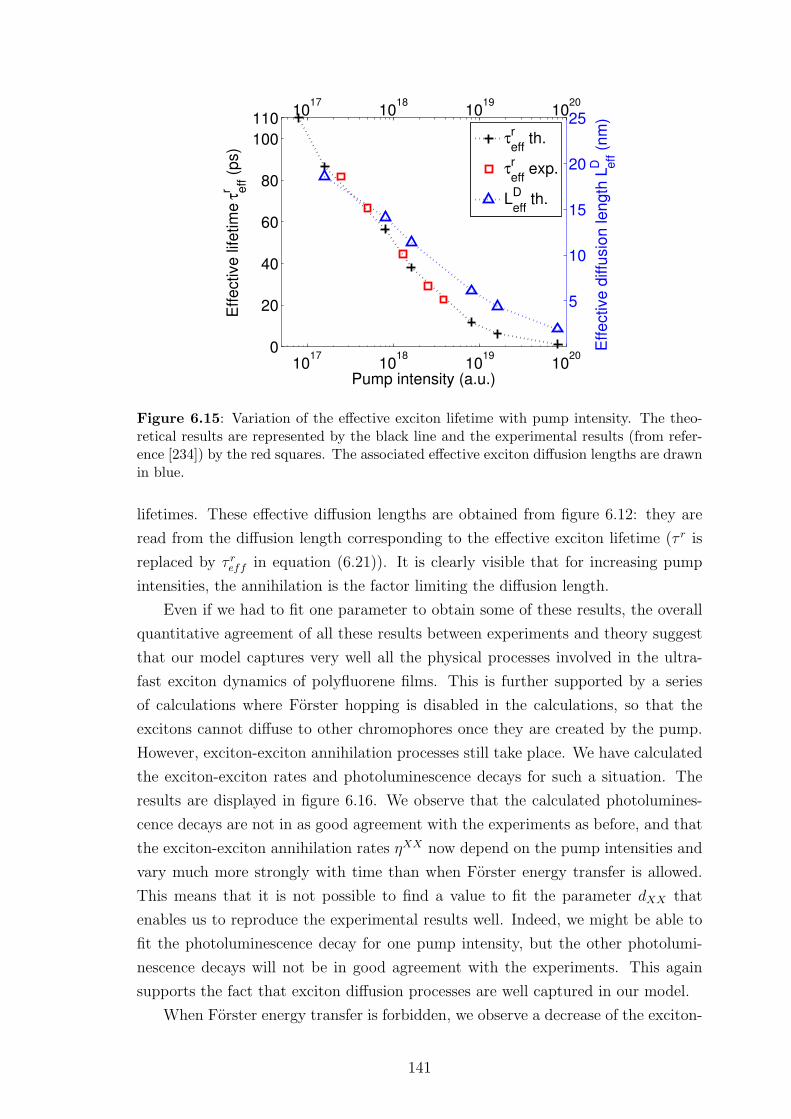
1017

1018

1019

1020

0

20

40

60

80

100

110

Pump intensity (a.u.)

Eff

ective

life

tim

e τ

eff

r (

ps)

τeff

r th.

τeff

r exp.

Leff

D th.

1017

1018

1019

1020

5

10

15

20

25

Eff

ective

diffu

sio

n le

ng

th L

eff

D (

nm

)

Figure 6.15: Variation of the effective exciton lifetime with pump intensity. The theo-retical results are represented by the black line and the experimental results (from refer-ence [234]) by the red squares. The associated effective exciton diffusion lengths are drawnin blue.

lifetimes. These effective diffusion lengths are obtained from figure 6.12: they are

read from the diffusion length corresponding to the effective exciton lifetime (τ r is

replaced by τ reff in equation (6.21)). It is clearly visible that for increasing pump

intensities, the annihilation is the factor limiting the diffusion length.

Even if we had to fit one parameter to obtain some of these results, the overall

quantitative agreement of all these results between experiments and theory suggest

that our model captures very well all the physical processes involved in the ultra-

fast exciton dynamics of polyfluorene films. This is further supported by a series

of calculations where Forster hopping is disabled in the calculations, so that the

excitons cannot diffuse to other chromophores once they are created by the pump.

However, exciton-exciton annihilation processes still take place. We have calculated

the exciton-exciton rates and photoluminescence decays for such a situation. The

results are displayed in figure 6.16. We observe that the calculated photolumines-

cence decays are not in as good agreement with the experiments as before, and that

the exciton-exciton annihilation rates ηXX now depend on the pump intensities and

vary much more strongly with time than when Forster energy transfer is allowed.

This means that it is not possible to find a value to fit the parameter dXX that

enables us to reproduce the experimental results well. Indeed, we might be able to

fit the photoluminescence decay for one pump intensity, but the other photolumi-

nescence decays will not be in good agreement with the experiments. This again

supports the fact that exciton diffusion processes are well captured in our model.

When Forster energy transfer is forbidden, we observe a decrease of the exciton-

141

0 20 40 60 80 1000

0.5

1

1.5

2

x 10−8

Time (ps)

XX

−a

nn

ihila

tio

n r

ate

η

XX (

cm

3/s

)

(b)

0 20 40 60 80 1000

0.2

0.4

0.6

0.8

1

Time (ps)

No

rma

lise

d P

L

(a)Low Power

I

2I

5.2I

10I

15.2I

Figure 6.16: Calculated (a) photoluminescence decays and (b) exciton-exciton annihila-tion rates ηXX for different pump intensities, when Forster energy transfer is forbidden inthe calculations. Theoretical data are represented by solid lines, experimental data (fromreference [234]) by dashed lines.

exciton annihilation rates ηXX . This decrease comes from the fact that once highly

populated neighbouring sites have been depleted by exciton-exciton annihilation,

no more annihilations occur in the system. In contrast, when Forster energy trans-

fer is allowed, the low energy, highly populated sites will receive excitons from

other sites as exciton-exciton annihilation occurs on these low energy sites, so that

exciton-exciton annihilation takes place at the same rate at any time. In agreement

with [234], this indicates that exciton-exciton annihilation is diffusion-controlled in

polyfluorene films. In such a case, the exciton-exciton annihilation rate ηXX can be

expressed as [234]:

ηXX = 4πRaD

(1 +

Ra√πDt

), (6.23)

where Ra is a constant (the “annihilation radius”). We notice that when Dt≫ Ra,

then ηXX is constant, but when Dt≪ Ra, ηXX decreases with time. The first case

corresponds to Forster hopping being enabled in our calculations, the second case

to Forster hopping being disabled.

Despite the lack of available methods to obtain the parameters involved in

exciton-exciton annihilation processes without fitting experimental results, we ob-

tained meaningful results and predictions of exciton-exciton annihilation processes

in polyfluorene films. In addition, these results further support the exciton dif-

fusion results we presented in Section 6.5, where exciton-exciton annihilation was

negligible, showing further evidence that exciton diffusion is well captured by our

model.

142

6.7 Conclusions

We have developed a flexible model to understand and simulate exciton dynam-

ics in films of linear chromophores. We have shown, by comparing the predictions

with anisotropy experiments, that sufficient parameters can be obtained from sim-

ple spectra and quantum chemistry to allow good agreement without requiring any

tuning parameters. Our model enables us to gain additional knowledge of exciton

transfer processes that are not accessible experimentally; for instance, that exci-

tons migrate directly to low energy chromophores and that, in consequence, energy-

matching plays a more important role than chromophore proximity in determining

the chromophore pairs where exciton transfer takes place. We have also extracted

the exciton diffusion length of such a film, the value being in very good agree-

ment with previously published experimental data. In addition, our model includes

exciton-exciton annihilation. Despite the lack of available methods to obtain the

parameters involved in exciton-exciton annihilation processes without fitting exper-

imental results, we obtained meaningful results and predictions of exciton-exciton

annihilation processes in polyfluorene films. These results show further evidence

that exciton diffusion is well captured by our model, and provides us with insight

on how Forster transfer plays a role in exciton-exciton annihilation processes.

143

Chapter 7

Conclusions and future work

We will conclude this thesis by summarising the most prominent results pre-

sented throughout these Chapters. We will then suggest some directions for future

research and some important questions that remain to be addressed to further in-

crease the understanding of the ultra-fast photo-dynamics of organic semiconductors,

on the basis of the knowledge we have gained through the work presented here.

7.1 Conclusions

We have given an introduction to organic semiconductors, and in particular to

their basic photo-physics, in Chapter 1. The importance of organic semiconductors

for the fabrication of a new generation of electronic devices has been presented,

in addition to the basic principles of the operation of these devices, with an em-

phasis on how the fundamental photo-physics properties of organic semiconductor

materials govern characteristics and performances of the device. This enabled us

to highlight the current challenges associated with molecular semiconducting mate-

rials. A theoretical description of exciton dynamics in real systems, that we could

compare to experimental data measured by our collaborators at the University of

St-Andrews, appeared to be a relevant way to address the fundamental challenges

of exciton dynamics in these materials. This description thus constitutes the focus

of the work presented in this thesis.

To develop successful models of exciton transfer in organic semiconductors, we

have utilised the methods we have presented in Chapter 2. We believe that the com-

bination of quantum chemistry methods, used at a level of theory which provides

good predictions of measurable quantities, with a model using a density-matrix ap-

proach for large systems (such as the optical Bloch equations (OBE)), can provide

good theoretical predictions of the exciton dynamics in molecular systems. Indeed,

we have demonstrated that quantum chemistry calculations can describe very ac-

curately single molecules properties, such as transition energies and dipoles, in flu-

orenes. Once these single-molecule properties are known, they can be used for the

time-dependent simulations of the exciton density of realistic ensembles of fluorenes,

the equations governing the system being derived from the OBE. However, we have

shown that calculations of a system of slightly more than a couple of molecules in

the framework of the OBE are not computationally tractable, and approximations

144

to the OBE will be needed to conduct large-scale simulations.

We have chosen to start our work with the study of a class of molecules with

known conformation in solution, where intra-molecular exciton transfer is likely

to happen: star-shaped molecules. More precisely, we investigated benzene- and

truxene-cored molecules, with three branched arms made of fluorene chains - the

length of these chains varying from zero to four fluorene units. Our theoretical results

were supported by experimental measurements of the transition dipoles and energies.

We found very good qualitative and quantitative agreement between our calculations

and the experiments, indicating that the theoretical results could be relied upon.

We gained valuable knowledge about the optical and electronic properties of these

molecules: we demonstrated that the C3-symmetry of the star-shaped molecules was

responsible for degenerate absorption states, resulting in uniform photo-excitation

all over the molecules (if excited by an isotropic light source). However, the excited-

state geometry cannot be symmetric, due to the shape of the excited state energy

potential, and as a consequence the excitation will necessarily relax to one of the

three arms of the molecule - the actual arm where excitation relaxes depending

on slight initial molecular conformal perturbations. This work was presented in

Chapter 3

It was nevertheless not clear from this study which arm the excitation will choose

to relax onto in the real star-shaped molecules. The time-scale of this relaxation pro-

cess was also not known, as it is impossible to calculate such a quantity by density

functional theory (DFT). In addition, incoherent exciton transfer between arms was

a possibility which could not be investigated by DFT either. This is why we con-

ducted a combined experimental and theoretical study of fluorescence anisotropy in

solutions of these star-shaped molecules, described in Chapter 4. We demonstrated

that the experimentally recorded fluorescence anisotropy could not correspond to

fluorescence anisotropy detected in C3-symmetric molecules, with degenerate ab-

sorption levels. We then proposed a theory to explain the measured fluorescence

anisotropy on the basis of quantum chemistry calculations. Indeed, the recorded

fluorescence anisotropy was what we would expect for non-degenerate “rod-like”

molecules; we demonstrated that symmetry-breaking defects exist at room tem-

perature, creating a splitting of the originally degenerate levels. This splitting is

large enough that the experimental pump pulse would excite only one of the two

absorption levels. By conducting a series of quantum chemistry calculations for a

variety of defects, we reached the conclusion that molecules with one absorption

energy lower than the original absorption levels would exhibit less depolarisation

due to molecular relaxation than molecules with higher absorption energies. This

was confirmed experimentally. In addition to the fast (hundreds of fs) anisotropy

decay due to molecular relaxation, we have assigned the slower (few ps) anisotropy

145

decay to excitation transfer between arms. This was supported by calculations of

the associated Forster rates.

Our work so far enabled us to gain more detailed knowledge of intra-molecular

excitation transfer in these fluorene-based molecules. However, inter-molecular pro-

cesses are also significant in organic films. In Chapter 5, we discussed the validity of

the point- and line- dipole models by comparing the interaction energies calculated

from these models for a series of configurations of pairs of oligofluorene molecules to

the interaction energy extracted from quantum chemistry calculations. We demon-

strated that even the line-dipole model could not accurately describe interactions at

separations and conformations typical of films. We proposed an improved version of

the line-dipole model which performs much better than the conventional line-dipole

model, and enables very accurate calculation of interactions for any configuration,

at the same low computational cost as the line-dipole model. Rather than using

a sinusoidal sub-dipole moment distribution of the length of half a period, our im-

proved model uses a sinusoidal distribution with a number of nodes and anti-nodes

to mimic more accurately the charge distribution of the excited molecules.

In Chapter 6, we used this improved line-dipole model to calculate the inter-

action energies in a randomly generated large ensemble of 125 000 chromophores.

These chromophores represent an ensemble of polyfluorene molecules, and are ap-

proximated as octamer oligofluorene molecules. The chromophores are randomly

positioned and oriented and their density is the same as the experimental mass den-

sity of a PF8 fluorene film. These chromophores also each possess their own absorp-

tion and emission energies, to mimic inhomogeneous broadening. This enables the

calculation of spectral overlaps between two chromophores, and therefore accurate

estimation of incoherent Forster hopping rates between any pairs of chromophores.

The parameters of this model are all fixed by quantum calculations or by experi-

mental measurements of the emission and absorption spectra. We can calculate the

fluorescence anisotropy of such a theoretical system. Comparison with experimental

measurements of fluorescence anisotropy recorded out of a PF8 polyfluorene film

shows very good agreement. In both cases, the observed anisotropy decay is very

fast, on the order of 680 fs, indicating ultra-fast excitation migration in the ensemble

of chromophores. We demonstrate that for this material, no mechanisms other than

incoherent Forster hopping need to be invoked to explain the observed anisotropy

decay, and that it is therefore the main mechanism governing measurable exciton

transfer at this time-scale. We also demonstrate that the excitation transfers di-

rectly to the low-energy molecules, and that consequently the sample morphology

plays a minor role in the exciton dynamics, with energy-matching (spectral over-

lap) having a much more significant role. In addition, we obtained exciton diffusion

length in very good agreement with previously published experimental data, and

146

we also account for exciton-exciton annihilation at high pump intensity - we can

reproduce the exciton lifetime variation with pump intensity very well. For all these

reasons, we believe the model we have developed is a new powerful tool to simulate

and understand further exciton dynamics mechanisms. The agreement of the ex-

perimental results with our theoretical predictions, showing sub-picosecond exciton

transfer in polyfluorene films, which had, to the best of our knowledge, never been

obtained prior to this research, strongly supports this.

7.2 Future work

With the validity of this exciton dynamics model having been demonstrated in

polyfluorene films, it would be extremely interesting to use this model to investigate

additional questions, such as how films of mixed different species behave, or what the

influence of more complex morphologies is on the exciton dynamics, and to extend

the model further. The research possibilities are numerous and would require an

extensive amount of work, and will hopefully be the subject of further investigation

in our group. As we have seen in the introductory Chapter, solar cells are made of

blends of materials, and the energy transfer dynamics in such systems is therefore

very complex. However it is crucial to know the diffusion properties of these devices

to ensure the most efficient collection of charges at the electrodes. It could therefore

be very helpful to be able to model diffusion in films of common blend of materials.

A way to achieve this would be, for instance, to start by simulating systems of mixed-

phase polyfluorenes (α- and β-phases). Indeed, this would be a simple extension to

the model (and is actually already almost implemented). The resulting predictions

would be easy to compare with already existing data for such a system, such as

measurements of exciton-exciton annihilation rates - because the β-phase molecules

are at much lower energy than the α-phase chromophores, they play the role of traps

and quench the excitation.

Once mixed film systems are successfully simulated, the study of the influence

of various possible morphologies on exciton dynamics will be of particular interest.

This could indeed help us understand, for instance, how molecular species are mixed

in such films, or how to improve the mixing to make the devices more efficient.

The model could also be extended to use more realistic sample morphologies.

In the work we have presented, we have used an ensemble of randomly oriented and

positioned chromophores to mimic an ensemble of polyfluorene molecules. A better

ensemble of chromophores could be generated using molecular dynamics simulations.

This would be more accurate as the chromophore sizes would be more realistic and

better positioned to mimic polyfluorene chains or the mixing of two different species,

for example. Comparison of exciton dynamics results from our model with other

147

experiments would also enable us to either confirm or refute the molecular dynamics

results.

Using quantum chemistry with quadratic response theory would also provide us

with theoretical excited-state absorption properties, and therefore exciton-exciton

annihilation would be simulated without fitting any parameters. This would greatly

enhance the model for high pump intensity cases. Similarly, having methods to cal-

culate homogeneous broadening would be useful and allow one to avoid the need for

experimental spectral data. Inhomogeneous broadening could possibly be obtained

by molecular dynamics. In this case, a model relying totally on theory would be

achieved, and no experiments would be necessary at all!

Additional physics mechanisms could also be included, for instance, coherent

energy transfer. However, in polyfluorenes, it seems that coherent effects would not

add much to the exciton dynamics at the 100 fs time-scale, and including coherences

in the equations would not be an easy task. We believe the reasons for including such

a mechanism are limited; however it would be useful to include other effects such

as the creation of polarons to model processes taking place in solar cells better and

free charges transport phenomena. Dexter transfer could be accounted for for the

studies of relevant materials, by the calculation of molecular orbitals by quantum

chemistry, and by the calculation of the subsequent molecular orbital overlaps -

there is currently no computationally tractable way of doing this to the best of our

knowledge.

It is clear that there are still lots of possibilities for further work to better

understand energy transfer in organic semiconductors, building from the basis of

the work we have presented in this thesis. In this context, the good results we

obtained from our model, compared to the experiments, is a very encouraging sign

that this research was focused in the right direction.

148

Appendix A

A.1 Spectral overlaps between two chromophores

Here we give the results needed for the evaluation of spectral overlaps between

Lorentzian lineshapes. If L(x, a) is a normalised Lorentzian:

L(x, a) =1

π

γ

γ2 + (x− a)2, (A.1)

centered at x = a, and of linewidth γ, then

∫ ∞

−∞

L(x, a) L(x, b) dx =2

π

γ

4γ2 + (a− b)2. (A.2)

If now the second lorentzian has the linewidth 2γ, the integral of the products is

3

π

γ

9γ2 + (a− b)2. (A.3)

These formulae are used to calculate the appropriate spectral overlaps.

A.2 Derivation of the source term

The Optical Bloch Equations (OBE) for a two-level system are [173]:

i~dp

dt= (−ε− iγ) p− (1− n)d ·E(t), (A.4)

~dn

dt= 2 Im [p d ·E∗(t)] , (A.5)

where p is the polarisation between the two levels, n is the excitation probabil-

ity (population of the higher level), γ the pure-dephasing, ε the energy difference

between the two levels, d the transition dipole and E the pumping optical field.

Defining E(t) = E(t)eiω0t and p(t) = p(t)eiω0t, with ~ω0 = ε and using the Rotat-

ing Wave Approximation (RWA) for a monochromatic source of angular frequency

ω0 (on resonance with the two-level system), then

E(t) =E0

2, (A.6)

149

and similarly for p. The OBE can therefore be rewritten as:

i~dp

dt= −iγp− (1− 2n)d · E(t), (A.7)

~dn

dt= 2Im

[pd · E∗(t)

]. (A.8)

With a monochromatic source of angular frequency ω0,dpdt

= 0 and therefore

p = i(1− 2n)d · E(t)/γ. The source term ρ = Im[pd · E∗(t)

]from the pump in the

equation for n is then such that

ρ ∝ (1− 2n)∣∣∣d · E(t)

∣∣∣2

. (A.9)

This is for a monochromatic source at angular frequency ω0. From the OBE we can

deduce the linear susceptibility χ(~ω):

χ(~ω) =P (~ω)

E(~ω)=

(1− 2n) d

~ω − ǫ− iγ. (A.10)

Therefore, a monochromatic source at the angular frequency ω, close to ω0, will

produce the following polarisation in the frequency domain:

P (~ω) =(1− 2n) d E(~ω)

~ω − ǫ− iγ. (A.11)

In such case:

ρ ∝(1− 2n)

∣∣∣d · E(t)∣∣∣2

γE(~ω)

(~ω − ǫ)2 + γ2, (A.12)

ρ ∝ (1− 2n)∣∣∣d · E(t)

∣∣∣2

A(~ω)E(~ω), (A.13)

For a non-monochromatic pump pulse of frequencies ω around ω0, the source term

can therefore be expressed as:

ρ ∝ (1− 2n)∣∣∣d · E(t)

∣∣∣2∫A(~ω)E(~ω)d(~ω). (A.14)

This, at low probability, is the expression we used in equation (6.7) of our model.

150

References

[1] B. Yacobi. Semiconductor Materials: An Introduction to Basic Principles, pp.

1–3. Springer, 2003.

[2] B. Bolto, R. McNeill, and D. Weiss. Electronic Conduction in Polymers. III.

Electronic Properties of Polypyrrole. Australian Journal of Chemistry 16(6),

1090–1103 (1963).

[3] T. H. Maiman. Stimulated Optical Radiation in Ruby. Nature 187(4736),

493–494 (1960).

[4] N. J. Holonyak and S. F. Bevacqua. Coherent (visible) light emission from

Ga(As1−xPx) junctions. Applied Physics Letters 1(4), 82–83 (1962).

[5] C. W. Tang and S. A. VanSlyke. Organic electroluminescent diodes. Applied

Physics Letters 51(12), 913–915 (1987).

[6] A. Tsumura, H. Koezuka, and T. Ando. Macromolecular electronic device:

Field-effect transistor with a polythiophene thin film. Applied Physics Letters

49(18), 1210–1212 (1986).

[7] M. Riordan, L. Hoddeson, and C. Herring. The invention of the transistor.

Reviews of Modern Physics 71, S336–S345 (1999).

[8] D. M. Chapin, C. S. Fuller, and G. L. Pearson. A New Silicon p-n Junction

Photocell for Converting Solar Radiation into Electrical Power. Journal of

Applied Physics 25(5), 676–677 (1954).

[9] C. W. Tang. Two-layer organic photovoltaic cell. Applied Physics Letters

48(2), 183–185 (1986).

[10] B. H. Soffer and B. B. McFarland. Continuously tunable, narrow-band organic

dye lasers. Applied Physics Letters 10(10), 266–267 (1967).

[11] N. Karl. Laser emission from an organic molecular crystal. Physica Status

Solidi A 13(2), 651–655 (1972).

[12] I. D. W. Samuel and G. A. Turnbull. Organic Semiconductor Lasers. Chemical

Reviews 107, 1272 (2007).

[13] D. Moses. High quantum efficiency luminescence from a conducting polymer

in solution: A novel polymer laser dye. Applied Physics Letters 60(26), 3215–

3216 (1992).

151

References 152

[14] W. Brutting. Physics of Organic Semiconductors. Wiley-VCH Verlag, 1st

edition, 2006.

[15] A. J. Heeger, S. Kivelson, J. R. Schrieffer, and W. P. Su. Solitons in conducting

polymers. Reviews of Modern Physics 60, 781–850 (1988).

[16] A. J. Heeger. Nobel Lecture: Semiconducting and metallic polymers: The

fourth generation of polymeric materials. Reviews of Modern Physics 73(14),

681–700 (2001).

[17] Wikimedia Commons. Data base of images in the public domain,

http://commons.wikimedia.org.

[18] S. Brazovskii and N. Kirova. Physical theory of excitons in conducting poly-

mers. Chemical Society Reviews 39, 2453–2465 (2010).

[19] A. Moliton and R. C. Hiorns. Review of electronic and optical properties of

semiconducting -conjugated polymers: applications in optoelectronics. Poly-

mer International 53(10), 1397–1412 (2004).

[20] N. Kirova, S. Brazovskii, and A. Bishop. A systematic theory for optical prop-

erties of phenylene-based polymers. Synthetic Metals 100(1), 29–53 (1999).

[21] M. Wohlgenannt, X. M. Jiang, Z. V. Vardeny, and R. A. J. Janssen.

Conjugation-Length Dependence of Spin-Dependent Exciton Formation Rates

in Π-Conjugated Oligomers and Polymers. Physical Review Letters 88, 197401

(2002).

[22] C. Kittel. Introduction to Solid State Physics. Willey, 1996.

[23] A. J. Heeger. Semiconducting polymers: the Third Generation. Chemical

Society Reviews 39, 2354–2371 (2010).

[24] J. D. Myers and J. Xue. Organic Semiconductors and their Applications in

Photovoltaic Devices. Polymer Reviews 52(1), 1–37 (2012).

[25] R. Knox. Theory of excitons. Academic Press, US, 1963.

[26] R. Smith. Semiconductors. University Press, Cambridge, 1978.

[27] S. F. Alvarado, P. F. Seidler, D. G. Lidzey, and D. D. C. Bradley. Direct

Determination of the Exciton Binding Energy of Conjugated Polymers Using

a Scanning Tunneling Microscope. Physical Review Letters 81, 1082–1085

(1998).

References 153

[28] M. Chandross, S. Mazumdar, M. Liess, P. A. Lane, Z. V. Vardeny, M. Ham-

aguchi, and K. Yoshino. Optical absorption in the substituted phenylene-based

conjugated polymers: Theory and experiment. Physical Review B 55, 1486–

1496 (1997).

[29] I. H. Campbell, T. W. Hagler, D. L. Smith, and J. P. Ferraris. Direct

Measurement of Conjugated Polymer Electronic Excitation Energies Using

Metal/Polymer/Metal Structures. Physical Review Letters 76, 1900–1903

(1996).

[30] V. May and O. Kuhn. Charge and Energy Transfer Dynamics in Molecular

Systems. Wiley-VCH, 2d, revised and enlarged edition, 2008.

[31] T. Nelson, S. Fernandez-Alberti, A. E. Roitberg, and S. Tretiak. Nonadiabatic

excited-state molecular dynamics: Treatment of electronic decoherence. The

Journal of Chemical Physics 138(22), 224111 (2013).

[32] I. Hwang and G. D. Scholes. Electronic Energy Transfer and Quantum-

Coherence in -Conjugated Polymers. Chemistry of Materials 23(3), 610–620

(2011).

[33] B. Kraabel, D. Moses, and A. J. Heeger. Direct observation of the intersystem

crossing in poly(3-octylthiophene). The Journal of Chemical Physics 103(12),

5102–5108 (1995).

[34] N. I. Nijegorodov and W. S. Downey. The Influence of Planarity and Rigidity

on the Absorption and Fluorescence Parameters and Intersystem Crossing

Rate Constant in Aromatic Molecules. The Journal of Physical Chemistry

98(22), 5639–5643 (1994).

[35] D. Beljonne, Z. Shuai, G. Pourtois, and J. L. Bredas. SpinOrbit Coupling and

Intersystem Crossing in Conjugated Polymers: A Configuration Interaction

Description. The Journal of Physical Chemistry A 105(15), 3899–3907 (2001).

[36] M. Yan, L. J. Rothberg, E. W. Kwock, and T. M. Miller. Interchain Excitations

in Conjugated Polymers. Physical Review Letters 75, 1992–1995 (1995).

[37] N. A. Montgomery, J.-C. Denis, S. Schumacher, A. Ruseckas, P. J. Skabara,

A. Kanibolotsky, M. J. Paterson, I. Galbraith, G. A. Turnbull, and I. D. W.

Samuel. Optical Excitations in Star-Shaped Fluorene Molecules. The Journal

of Physical Chemistry A 115(14), 2913–2919 (2011).

[38] D. Beljonne, G. Pourtois, C. Silva, E. Hennebicq, L. M. Herz, R. H. Friend,

G. D. Scholes, S. Setayesh, K. Mu, and J. L. Bre. Interchain vs . intrachain

References 154

energy transfer in acceptor-. Proceedings of the National Academy of Sciences

99(17), 10982 (2002).

[39] J. Franck and R. Livingston. Remarks on Intra- and Inter-Molecular Migration

of Excitation Energy. Reviews of Modern Physics 21, 505–509 (1949).

[40] T. Forster. 10th Spiers Memorial Lecture. Transfer mechanisms of electronic

excitation. Discussions of the Faraday Society 27, 7–17 (1959).

[41] R. M. Clegg. Forster resonance energy transfer—FRET what is it, why do it,

and how it’s done. In T. Gadella, editor, Fret and Flim Techniques, volume 33

of Laboratory Techniques in Biochemistry and Molecular Biology, pp. 1–57.

Elsevier, 2009.

[42] A. Olaya-Castro and G. D. Scholes. Energy transfer from Forster–Dexter the-

ory to quantum coherent light-harvesting. International Reviews in Physical

Chemistry 30(1), 49–77 (2011).

[43] G. D. Scholes. Long-range resonance energy transfer in molecular systems.

Annual Review of Physical Chemistry 54(1), 57–87 (2003).

[44] T. Forster. Zwischenmolekulare Energiewanderung und Fluoreszenz. Annalen

der Physik 437(1-2), 55–75 (1948).

[45] G. D. Scholes, X. J. Jordanides, and G. R. Fleming. Adapting the Forster

Theory of Energy Transfer for Modeling Dynamics in Aggregated Molecular

Assemblies. The Journal of Physical Chemistry B 105(8), 1640–1651 (2001).

[46] D. L. Dexter. A Theory of Sensitized Luminescence in Solids. The Journal of

Chemical Physics 21(5), 836–850 (1953).

[47] R. D. Jenkins, G. J. Daniels, and D. L. Andrews. Quantum pathways for

resonance energy transfer. The Journal of Chemical Physics 120(24), 11442–

11448 (2004).

[48] G. D. Scholes and D. L. Andrews. Damping and higher multipole effects in

the quantum electrodynamical model for electronic energy transfer in the con-

densed phase. The Journal of Chemical Physics 107(14), 5374–5384 (1997).

[49] D. Andrews. A unified theory of radiative and radiationless molecular energy

transfer. Chemical Physics 135(2), 195–201 (1989).

[50] A. Czader and E. R. Bittner. Calculations of the exciton coupling elements

between the DNA bases using the transition density cube method. The Journal

of Chemical Physics 128(3), 035101 (2008).

References 155

[51] B. P. Krueger, G. D. Scholes, and G. R. Fleming. Calculation of Couplings and

Energy-Transfer Pathways between the Pigments of LH2 by the ab Initio Tran-

sition Density Cube Method. The Journal Physical Chemistry B 5647(98),

5378–5386 (1998).

[52] G. D. Scholes and G. R. Fleming. Energy Transfer and Photosynthetic Light

Harvesting, pp. 57–129. John Wiley & Sons, Inc., 2005.

[53] G. D. Scholes and K. P. Ghiggino. Electronic Interactions and Interchro-

mophore Excitation Transfer. The Journal of Physical Chemistry 98(17),

4580–4590 (1994).

[54] V. May. Beyond the Forster theory of excitation energy transfer: importance

of higher-order processes in supramolecular antenna systems. Dalton Trans-

actions , 10086–10105 (2009).

[55] G. J. Daniels, R. D. Jenkins, D. S. Bradshaw, and D. L. Andrews. Resonance

energy transfer: The unified theory revisited. The Journal of Chemical Physics

119(4), 2264–2274 (2003).

[56] D. Onidas, T. Gustavsson, E. Lazzarotto, and D. Markovitsi. Fluorescence of

the DNA Double Helix (dA)20(dT)20 Studied by Femtosecond Spectroscopy-

Effect of the Duplex Size on the Properties of the Excited States. The Journal

of Physical Chemistry B 111(32), 9644–9650 (2007).

[57] B. Fuckel, A. Kohn, M. E. Harding, G. Diezemann, G. Hinze, T. Basche, and

J. Gauss. Theoretical investigation of electronic excitation energy transfer in

bichromophoric assemblies. The Journal of Chemical Physics 128(7), 074505

(2008).

[58] C.-P. Hsu, G. R. Fleming, M. Head-Gordon, and T. Head-Gordon. Excitation

energy transfer in condensed media. The Journal of Chemical Physics 114(7),

3065–3072 (2001).

[59] A. Nazir. Correlation-Dependent Coherent to Incoherent Transitions in Reso-

nant Energy Transfer Dynamics. Physical Review Letters 103, 146404 (2009).

[60] M. Grover and R. Silbey. Exciton Migration in Molecular Crystals. The

Journal of Chemical Physics 54(11), 4843–4851 (1971).

[61] B. Jackson and R. Silbey. On the calculation of transfer rates between impurity

states in solids. The Journal of Chemical Physics 78(6), 4193–4196 (1983).

References 156

[62] I. Franco, M. Shapiro, and P. Brumer. Femtosecond dynamics and laser control

of charge transport in trans-polyacetylene. The Journal of Chemical Physics

128(24), 244905 (2008).

[63] O. V. Prezhdo and P. J. Rossky. Relationship between Quantum Decoher-

ence Times and Solvation Dynamics in Condensed Phase Chemical Systems.

Physical Review Letters 81, 5294–5297 (1998).

[64] H. Hwang and P. J. Rossky. Electronic Decoherence Induced by Intramolecular

Vibrational Motions in a Betaine Dye Molecule. The Journal of Physical

Chemistry B 108(21), 6723–6732 (2004).

[65] O. Varnavski, I. D. W. Samuel, L.-O. Palsson, R. Beavington, P. L. Burn, and

T. G. III. Investigations of excitation energy transfer and intramolecular in-

teractions in a nitrogen corded distrylbenzene dendrimer system. The Journal

of Chemical Physics 116(20), 8893–8903 (2002).

[66] D. C. Arnett, C. C. Moser, P. L. Dutton, and N. F. Scherer. The First Events

in Photosynthesis: Electronic Coupling and Energy Transfer Dynamics in the

Photosynthetic Reaction Center from Rhodobacter sphaeroides. The Journal

of Physical Chemistry B 103(11), 2014–2032 (1999).

[67] S. Savikhin, D. R. Buck, and W. S. Struve. Oscillating anisotropies in a

bacteriochlorophyll protein: Evidence for quantum beating between exciton

levels. Chemical Physics 223(2–3), 303–312 (1997).

[68] T. Goodson. Time-resolved spectroscopy of organic dendrimers and branched

chromophores. Annual Review of Physical Chemistry 56(1), 581–603 (2005).

[69] T. Kakitani, A. Kimura, and H. Sumi. Theory of Excitation Transfer in the

Intermediate Coupling Case. The Journal of Physical Chemistry B 103(18),

3720–3726 (1999).

[70] K. M. Gaab and C. J. Bardeen. The effects of connectivity, coherence, and

trapping on energy transfer in simple light-harvesting systems studied using

the Haken-Strobl model with diagonal disorder. The Journal of Chemical

Physics 121(16), 7813–7820 (2004).

[71] J. Cao and R. J. Silbey. Optimization of Exciton Trapping in Energy Transfer

Processes. The Journal of Physical Chemistry A 113(50), 13825–13838 (2009).

[72] J. S. Swensen, C. Soci, and A. J. Heeger. Light emission from an ambipolar

semiconducting polymer field-effect transistor. Applied Physics Letters 87(25),

253511–253513 (2005).

References 157

[73] X. Gong, M. Tong, Y. Xia, W. Cai, J. S. Moon, Y. Cao, G. Yu, C.-L. Shieh,

B. Nilsson, and A. J. Heeger. High-Detectivity Polymer Photodetectors with

Spectral Response from 300 nm to 1450 nm. Science 325(5948), 1665–1667

(2009).

[74] N. S. Sariciftci, L. Smilowitz, A. J. Heeger, and F. Wudl. Photoinduced Elec-

tron Transfer from a Conducting Polymer to Buckminsterfullerene. Science

258(5087), 1474–1476 (1992).

[75] A. E. Siegman. Lasers. University Science Books, 1986.

[76] O. S. Avanesjan, V. A. Benderskii, V. K. Brikenstein, V. L. Broude, L. I.

Korshunov, A. G. Lavrushko, and I. I. Tartakovskii. Anthracene Crystals

Under Intensive Optical Pumping. Molecular Crystals and Liquid Crystals

29(1), 165–174 (1974).

[77] M. A. Dıaz-Garcıa, F. Hide, B. J. Schwartz, M. D. McGehee, M. R. Anders-

son, and A. J. Heeger. “Plastic” lasers: Comparison of gain narrowing with

a soluble semiconducting polymer in waveguides and microcavities. Applied

Physics Letters 70(24), 3191–3193 (1997).

[78] R. H. Friend, G. J. Denton, N. Tessler, and M. A. Stevens. Spectral narrowing

in optically pumped poly (p-phenylenevinylene) Films. Advanced Materials

9(7), 547–551 (1997).

[79] G. Heliotis, R. Xia, D. D. C. Bradley, G. A. Turnbull, I. D. W. Samuel,

P. Andrew, and W. L. Barnes. Blue, surface-emitting, distributed feedback

polyfluorene lasers. Applied Physics Letters 83, 2118 (2003).

[80] J. R. Lawrence, G. A. Turnbull, I. D. W. Samuel, G. J. Richards, and P. L.

Burn. Optical amplification in a first-generation dendriticorganic semiconduc-

tor. Optics Letters 29(8), 869–871 (2004).

[81] G. Tsiminis, J.-C. Ribierre, A. Ruseckas, H. S. Barcena, G. J. Richards, G. A.

Turnbull, P. L. Burn, and I. D. W. Samuel. Two-Photon Absorption and Las-

ing in First-Generation Bisfluorene Dendrimers. Advanced Materials 20(10),

1940–1944 (2008).

[82] G. Tsiminis, Y. Wang, P. E. Shaw, A. L. Kanibolotsky, I. F. Perepichka, M. D.

Dawson, P. J. Skabara, G. A. Turnbull, and I. D. W. Samuel. Low-threshold

organic laser based on an oligofluorene truxene with low optical losses. Applied

Physics Letters 94(24), 243304 (2009).

References 158

[83] S. V. Frolov, W. Gellermann, M. Ozaki, K. Yoshino, and Z. V. Vardeny.

Cooperative Emission in π-Conjugated Polymer Thin Films. Physical Review

Letters 78, 729–732 (1997).

[84] G. Cerullo, S. Stagira, M. Nisoli, S. De Silvestri, G. Lanzani, G. Kranzel-

binder, W. Graupner, and G. Leising. Excited-state dynamics of poly(para-

phenylene)-type ladder polymers at high photoexcitation density. Physical

Review B 57, 12806–12811 (1998).

[85] N. Tessler, G. J. Denton, and R. H. Friend. Lasing from conjugated-polymer

microcavities. Nature 382(6593), 695–697 (1996).

[86] V. D. Mihailetchi, J. Wildeman, and P. W. M. Blom. Space-Charge Limited

Photocurrent. Physical Review Letters 94, 126602 (2005).

[87] V. G. Kozlov, V. Bulovic, and S. R. Forrest. Temperature independent per-

formance of organic semiconductor lasers. Applied Physics Letters 71(18),

2575–2577 (1997).

[88] G. Wegmann, H. Giessen, A. Greiner, and R. F. Mahrt. Laser emission from a

solid conjugated polymer: Gain, tunability, and coherence. Physical Review

B 57, R4218–R4221 (1998).

[89] G. Turnbull, T. Krauss, W. Barnes, and I. Samuel. Tuneable distributed

feedback lasing in MEH-PPV films. Synthetic Metals 121(1–3), 1757–1758

(2001).

[90] R. R. King, D. C. Law, K. M. Edmondson, C. M. Fetzer, G. S. Kinsey, H. Yoon,

R. A. Sherif, and N. H. Karam. 40% efficient metamorphic GaInP/GaInAs/Ge

multijunction solar cells. Applied Physics Letters 90(18), 183516 (2007).

[91] M. Scharber and N. Sariciftci. Efficiency of bulk-heterojunction organic solar

cells. Progress in Polymer Science 38(12), 1929–1940 (2013).

[92] M. A. Green, K. Emery, Y. Hishikawa, W. Warta, and E. D. Dunlop. Solar

cell efficiency tables (version 39). Progress in Photovoltaics: Research and

Applications 20(1), 12–20 (2012).

[93] W. Cai, X. Gong, and Y. Cao. Polymer solar cells: Recent development and

possible routes for improvement in the performance. Solar Energy Materials

and Solar Cells 94(2), 114–127 (2010).

[94] T. Singh, N. Marjanovic, G. Matt, S. Gunes, N. Sariciftci, A. M. Ramil,

A. Andreev, H. Sitter, R. Schwodiauer, and S. Bauer. High-mobility n-channel

References 159

organic field-effect transistors based on epitaxially grown C60 films. Organic

Electronics 6(3), 105–110 (2005).

[95] P. W. M. Blom, V. D. Mihailetchi, L. J. A. Koster, and D. E. Markov. De-

vice Physics of Polymer:Fullerene Bulk Heterojunction Solar Cells. Advanced

Materials 19(12), 1551–1566 (2007).

[96] H. Hoppe and N. S. Sariciftci. Organic solar cells: An overview. Journal of

Materials Research 19, 1924–1945 (2004).

[97] W. A. Luhman and R. J. Holmes. Investigation of Energy Transfer in Organic

Photovoltaic Cells and Impact on Exciton Diffusion Length Measurements.

Advanced Functional Materials 21(4), 764–771 (2011).

[98] P. Peumans, S. Uchida, and S. R. Forrest. Efficient bulk heterojunction

photovoltaic cells using small-molecular-weight organic thin films. Nature

425(6954), 158–162 (2003).

[99] O. A. Abdulrazzaq, V. Saini, S. Bourdo, E. Dervishi, and A. S. Biris. Or-

ganic Solar Cells: A Review of Materials, Limitations, and Possibilities for

Improvement. Particulate Science and Technology 31(5), 427–442 (2013).

[100] W. Helfrich and W. G. Schneider. Recombination Radiation in Anthracene

Crystals. Physical Review Letters 14, 229–231 (1965).

[101] J. H. Burroughes, D. D. C. Bradley, A. R. Brown, R. N. Marks, K. Mackay,

R. H. Friend, P. L. Burns, and A. B. Holmes. Light-emitting diodes based on

conjugated polymers. Nature 347(6293), 539–541 (1990).

[102] B. W. D’Andrade and S. R. Forrest. White Organic Light-Emitting Devices

for Solid-State Lighting. Advanced Materials 16(18), 1585–1595 (2004).

[103] Y.-S. Tyan. Organic light-emitting-diode lighting overview. Journal of Pho-

tonics for Energy 1(1), 011009–011009–15 (2011).

[104] G. Schwartz, S. Reineke, T. C. Rosenow, K. Walzer, and K. Leo. Triplet Har-

vesting in Hybrid White Organic Light-Emitting Diodes. Advanced Functional

Materials 19(9), 1319–1333 (2009).

[105] M. C. Gather, A. Kohnen, and K. Meerholz. White Organic Light-Emitting

Diodes. Advanced Materials 23(2), 233–248 (2011).

[106] W. Brutting, J. Frischeisen, T. D. Schmidt, B. J. Scholz, and C. Mayr. De-

vice efficiency of organic light-emitting diodes: Progress by improved light

outcoupling. Physica Status Solidi A 210(1), 44–65 (2013).

References 160

[107] S. Reineke, M. Thomschke, B. Lussem, and K. Leo. White organic light-

emitting diodes: Status and perspective. Reviews of Modern Physics 85, 1245–

1293 (2013).

[108] M. A. Baldo, D. F. O’Brien, M. E. Thompson, and S. R. Forrest. Excitonic

singlet-triplet ratio in a semiconducting organic thin film. Physical Review B

60, 14422–14428 (1999).

[109] M. A. Baldo, O. D. F., Y. You, A. Shoustikov, S. Sibley, M. E. Thompson,

and S. R. Forrest. Highly efficient phosphorescent emission from organic elec-

troluminescent devices. Nature 395(6698), 151–154 (1998).

[110] B. Wang, G. Helander, J. Qiu, P. Puzzo, T. Greiner, M. Hudson, S. Wang,

W. Liu, and H. Lu. Unlocking the full potential of organic light-emitting

diodes on flexible plastic. Nature Photonics 5(12), 753–757 (2011).

[111] S. Reineke, F. Lindner, G. Schwartz, N. Seidler, K. Walzer, B. Lussem, and

K. Leo. White organic light-emitting diodes with fluorescent tube efficiency.

Nature 459(7244), 234–238 (2009).

[112] L. Xiao, Z. Chen, B. Qu, J. Luo, S. Kong, Q. Gong, and J. Kido. Recent Pro-

gresses on Materials for Electrophosphorescent Organic Light-Emitting De-

vices. Advanced Materials 23(8), 926–952 (2011).

[113] J. Kido, H. Hayase, K. Hongawa, K. Nagai, and K. Okuyama. Bright red

light-emitting organic electroluminescent devices having a europium complex

as an emitter. Applied Physics Letters 65(17), 2124–2126 (1994).

[114] F. So and D. Kondakov. Degradation Mechanisms in Small-Molecule and

Polymer Organic Light-Emitting Diodes. Advanced Materials 22(34), 3762–

3777 (2010).

[115] Royal Society of Chemistry. Organic Electronics for a Better Tomorrow: Inno-

vation, Accessibility, Sustainability. Technical report, Royal Society of Chem-

istry, 2012.

[116] N. C. Miller, E. Cho, R. Gysel, C. Risko, V. Coropceanu, C. E. Miller, S. Sweet-

nam, A. Sellinger, M. Heeney, I. McCulloch, J.-L. Bredas, M. F. Toney, and

M. D. McGehee. Factors Governing Intercalation of Fullerenes and Other

Small Molecules Between the Side Chains of Semiconducting Polymers Used

in Solar Cells. Advanced Energy Materials 2(10), 1208–1217 (2012).

References 161

[117] V. N. Gorshkov, S. Tretiak, and D. Mozyrsky. Semiclassical Monte-Carlo

approach for modelling non-adiabatic dynamics in extended molecules. Nature

Communications 4 (2013).

[118] J. Cabanillas-Gonzalez, G. Grancini, and G. Lanzani. Pump-Probe Spec-

troscopy in Organic Semiconductors: Monitoring Fundamental Processes of

Relevance in Optoelectronics. Advanced Materials 23(46), 5468–5485 (2011).

[119] J. Clark, T. Nelson, S. Tretiak, G. Cirmi, and G. Lanzani. Femtosecond

torsional relaxation. Nature Physics 8(3), 225–231 (2012).

[120] D. A. Vithanage, A. Devizis, V. Abramavicius, Y. Infahsaeng, D. Abra-

mavicius, R. C. I. MacKenzie, P. E. Keivanidis, A. Yartsev, D. Hertel, J. Nel-

son, V. Sundstrom, and V. Gulbinas. Visualizing charge separation in bulk

heterojunction organic solar cells. Nature Communications 4 (2013).

[121] K. Ishii, S. Nakanishi, and N. Tsurumachi. Ultrafast transition between polari-

ton doublet and alternating current Stark triplet in organic one-dimensional

photonic crystal microcavity. Applied Physics Letters 103(1), 13301–13303

(2013).

[122] N. Banerji. Sub-picosecond delocalization in the excited state of conjugated

homopolymers and donor-acceptor copolymers. J. Mater. Chem. C 1, 3052–

3066 (2013).

[123] S. Ling, S. Schumacher, I. Galbraith, and M. J. Paterson. Excited-State Ab-

sorption of Conjugated Polymers in the Near-Infrared and Visible: A Com-

putational Study of Oligofluorenes. The Journal of Physical Chemistry C

117(13), 6889–6895 (2013).

[124] F. Jensen. Introduction to Computational Chemistry. Wiley-VCH Verlag,

1999.

[125] S. Schumacher, I. Galbraith, A. Ruseckas, G. A. Turnbull, and I. D. W.

Samuel. Dynamics of photoexcitation and stimulated optical emission in

conjugated polymers: A multiscale quantum-chemistry and Maxwell-Bloch-

equations approach. Physical Review B 81, 245407 (2010).

[126] H. Bassler. Charge Transport in Disordered Organic Photoconductors a Monte

Carlo Simulation Study. physica status solidi (b) 175(1), 15–56 (1993).

[127] S. C. J. Meskers, J. Hubner, M. Oestreich, and H. Bassler. Dispersive Relax-

ation Dynamics of Photoexcitations in a Polyfluorene Film Involving Energy

References 162

Transfer: Experiment and Monte Carlo Simulations. The Journal of Physical

Chemistry B 105(38), 9139–9149 (2001).

[128] P. K. Watkins, A. B. Walker, and G. L. B. Verschoor. Dynamical Monte

Carlo Modelling of Organic Solar Cells: The Dependence of Internal Quantum

Efficiency on Morphology. Nano Letters 5(9), 1814–1818 (2005).

[129] C. Groves and N. Greenham. Monte Carlo Simulations of Organic Photo-

voltaics. In Topics in Current Chemistry 2013, Topics in Current Chemistry,

pp. 1–22. Springer Berlin Heidelberg, 2013.

[130] D. Mendels and N. Tessler. Drift and Diffusion in Disordered Organic Semi-

conductors: The Role of Charge Density and Charge Energy Transport. The

Journal of Physical Chemistry C 117(7), 3287–3293 (2013).

[131] M. Mesta, M. Carvelli, J. de Vries Rein, H. van Eersel, M. van der Holst,

J. Jeroen, M. Schober, M. Furno, B. Lussem, K. Leo, P. Loebl, R. Coehoorn,

and P. A. Bobbert. Molecular-scale simulation of electroluminescence in a mul-

tilayer white organic light-emitting diode. Nat Mater 12(7), 652–658 (2013).

[132] L. Meng, Y. Shang, Q. Li, Y. Li, X. Zhan, Z. Shuai, R. G. E. Kimber, and

A. B. Walker. Dynamic Monte Carlo simulation for highly efficient polymer

blend photovoltaics. The Journal Physical Chemistry B 114(1), 36–41 (2010).

[133] S. Athanasopoulos, E. V. Emelianova, A. B. Walker, and D. Beljonne. Exci-

ton diffusion in energetically disordered organic materials. Physical Review B

80(19), 1–7 (2009).

[134] C. Daniel, S. Westenhoff, F. Makereel, R. H. Friend, D. Beljonne, L. M. Herz,

and C. Silva. Monte Carlo Simulation of Exciton Bimolecular Annihilation Dy-

namics in Supramolecular Semiconductor Architectures. The Journal Physical

Chemistry C 111(51), 19111–19119 (2007).

[135] M. Grage, Y. Zaushitsyn, A. Yartsev, M. Chachisvilis, V. Sundstrom, and

T. o. Pullerits. Ultrafast excitation transfer and trapping in a thin polymer

film. Physical Review B 67(20), 1–5 (2003).

[136] O. R. Tozer and W. Barford. Exciton Dynamics in Disordered Poly(p-

phenylenevinylene). 1. Ultrafast Interconversion and Dynamical Localization.

The Journal of Physical Chemistry A 116(42), 10310–10318 (2012).

[137] V. M. Kenkre. The master equation approach: Coherence, energy transfer,

annihilation, and relaxation. Springer Berlin Heidelberg, 1982.

References 163

[138] M. Yang and G. R. Fleming. Influence of phonons on exciton transfer dy-

namics: comparison of the Redfield, Forster, and modified Redfield equations.

Chemical Physics 282(1), 163–180 (2002).

[139] D. Marx and J. Hutter. Ab Initio Molecular Dynamics: Basic Theory and

Advanced Methods. Cambridge University Press, 2009.

[140] M. Levitt. Protein folding by restrained energy minimization and molecular

dynamics. Journal of Molecular Biology 170(3), 723–764 (1983).

[141] M. Karplus and J. A. McCammon. Molecular dynamics simulations of

biomolecules. Nature Structural & Molecular Biology 9(9), 646–652 (2002).

[142] A. Jabbarzadeh and R. I. Tanner. Molecular dynamics simulation and its

application to nano-rheology. Rheology Reviews , 165–216 (2006).

[143] J. Kohanoff. Electronic Structure Calculations for Solids and Molecules. The-

ory and Computational Methods. Cambridge University Press, 2006.

[144] J. B. Foresman and E. Frisch. Exploring Chemistry with Electronic Structure

Methods. Gaussian Inc., 2nd edition, 1996.

[145] N. C. Handy and A. M. Lee. The adiabatic approximation. Chemical Physics

Letters 252(5–6), 425–430 (1996).

[146] M. Born and R. Oppenheimer. Zur Quantentheorie der Molekeln. Annalen

der Physik 389(20), 457–484 (1927).

[147] P. Hohenberg. Inhomogeneous Electron Gas. Physical Review 136(3B), B864–

B871 (1964).

[148] W. Kohn. Self-Consistent Equations Including Exchange and Correlation Ef-

fects. Physical Review 140(4A), A1133–A1138 (1965).

[149] M. A. Marques, C. A. Ullrich, F. Nogueira, A. Rubio, K. Burke, and E. K. U.

Gross. Time-Dependent Density Functional Theory. Springer Berlin Heidel-

berg, 2006.

[150] C. A. Ullrich and Z.-H. Yang. A Brief Compendium of Time-Dependent Den-

sity Functional Theory. Brazilian Journal of Physics , 1–35 (2013).

[151] R. Van Leeuwen. Key concepts in time-dependent density-functional theory.

International Journal of Modern Physics B 15(14), 1969–2023 (2001).

[152] E. Runge and E. K. U. Gross. Density-Functional Theory for Time-Dependent

Systems. Physical Review Letters 52, 997–1000 (1984).

References 164

[153] A. D. Becke. Density-functional exchange-energy approximation with correct

asymptotic behavior. Physical Review A 38, 3098–3100 (1988).

[154] C. Lee, W. Yang, and R. G. Parr. Development of the Colle-Salvetti

correlation-energy formula into a functional of the electron density. Physi-

cal Review B 37, 785–789 (1988).

[155] A. D. Becke. Densityfunctional thermochemistry. III. The role of exact ex-

change. Journal of Chemical Physics 98(7), 5648–5652 (1992).

[156] T. Yanai, D. P. Tew, and N. C. Handy. A new hybrid exchange–correlation

functional using the Coulomb-attenuating method (CAM-B3LYP). Chemical

Physics Letters 393(1–3), 51–57 (2004).

[157] Y. Zhao and D. Truhlar. The M06 suite of density functionals for main group

thermochemistry, thermochemical kinetics, noncovalent interactions, excited

states, and transition elements: two new functionals and systematic testing

of four M06-class functionals and 12 other functionals. Theoretical Chemistry

Accounts 120(1-3), 215–241 (2008).

[158] W. J. Hehre, R. F. Stewart, and J. A. Pople. Self-Consistent Molecular-Orbital

Methods. I. Use of Gaussian Expansions of Slater-Type Atomic Orbitals. The

Journal of Chemical Physics 51(6), 2657–2664 (1969).

[159] P. Hariharan and J. Pople. The influence of polarization functions on molecular

orbital hydrogenation energies. Theoretica chimica acta 28(3), 213–222 (1973).

[160] M. J. Frisch, J. A. Pople, and J. S. Binkley. Self-consistent molecular orbital

methods 25. Supplementary functions for Gaussian basis sets. The Journal of

Chemical Physics 80(7), 3265–3269 (1984).

[161] T. Clark, J. Chandrasekhar, G. W. Spitznagel, and P. V. R. Schleyer. Efficient

diffuse function-augmented basis sets for anion calculations. III. The 3-21+G

basis set for first-row elements, Li–F. Journal of Computational Chemistry

4(3), 294–301 (1983).

[162] Gaussian09 User’s Reference.

[163] S. Schumacher, A. Ruseckas, N. A. Montgomery, P. J. Skabara, A. L. Kani-

bolotsky, M. J. Paterson, I. Galbraith, G. A. Turnbull, and I. D. W. Samuel.

Effect of exciton self-trapping and molecular conformation on photophysical

properties of oligofluorenes. The Journal of Chemical Physics 131, 154906

(2009).

References 165

[164] M. J. Frisch, G. W. Trucks, H. B. Schlegel, G. E. Scuseria, M. A. Robb, J. R.

Cheeseman, G. Scalmani, V. Barone, B. Mennucci, G. A. Petersson, H. Nakat-

suji, M. Caricato, X. Li, H. P. Hratchian, A. F. Izmaylov, J. Bloino, G. Zheng,

J. L. Sonnenberg, M. Hada, M. Ehara, K. Toyota, R. Fukuda, J. Hasegawa,

M. Ishida, T. Nakajima, Y. Honda, O. Kitao, H. Nakai, T. Vreven, J. J. A.

Montgomery, J. E. Peralta, F. Ogliaro, M. Bearpark, J. J. Heyd, E. Brothers,

K. N. Kudin, V. N. Staroverov, R. Kobayashi, J. Normand, K. Raghavachari,

A. Rendell, J. C. Burant, S. S. Iyengar, J. Tomasi, M. Cossi, N. Rega,

J. M. Millam, M. Klene, J. E. Knox, J. B. Cross, V. Bakken, C. Adamo,

J. Jaramillo, R. Gomperts, R. E. Stratmann, O. Yazyev, A. J. Austin,

R. Cammi, C. Pomelli, J. W. Ochterski, R. L. Martin, K. Morokuma, V. G.

Zakrzewski, G. A. Voth, P. Salvador, J. J. Dannenberg, S. Dapprich, A. D.

Daniels, O. Farkas, J. B. Foresman, J. V. Ortiz, J. Cioslowski, and D. J. Fox.

Gaussian 09 Revision A.1, 2009. Gaussian Inc. Wallingford CT 2009.

[165] W. J. Hehre, W. A. Lathan, R. Ditchfield, M. D. Newton, and J. A. Pople.

Gaussian 70, 1970. Quantum Chemistry Program Exchange, Program No.

237.

[166] R. Dennington, T. Keith, and J. Millam. GaussView Version 5, 2009.

Semichem Inc. Shawnee Mission KS 2009.

[167] K. Sriwichitkamol, S. Suramitr, P. Poolmee, and S. Hannongbua. Structures,

absorption spectra, and electronic properties of polyfluorene and its deriva-

tives: a theoretical study. Journal of Theoretical and Computational Chem-

istry 05(03), 595–608 (2006).

[168] E. Jansson, P. C. Jha, and H. Agren. Chain length dependence of singlet and

triplet excited states of oligofluorenes: A density functional study. Chemical

Physics 336(2–3), 91–98 (2007).

[169] K. I. Igumenshchev, S. Tretiak, and V. Y. Chernyak. Excitonic effects in a

time-dependent density functional theory. The Journal of Chemical Physics

127(11), 114902 (2007).

[170] V. Marcon, N. van der Vegt, G. Wegner, and G. Raos. Modeling of Molec-

ular Packing and Conformation in Oligofluorenes. The Journal of Physical

Chemistry B 110(11), 5253–5261 (2006).

[171] U. Scherf and D. Neher, editors. Polyfluorenes, volume 212 of Advances in

polymer science. Springer, Berlin, 2008.

References 166

[172] C. Cohen-Tannoudji, J. Dupont-Roc, and G. Grynberg. Optical Bloch Equa-

tions, pp. 353–405. Wiley-VCH Verlag GmbH, 2008.

[173] L. Allen and J. H. Eberly. Optical Resonance and Two-Level Atoms. Dover

Publications, soft cover edition, 1987.

[174] M. Lindberg and S. W. Koch. Effective Bloch equations for semiconductors.

Physical Review B 38, 3342–3350 (1988).

[175] S. Mukamel. Principles of Nonlinear Optical Spectroscopy (Oxford Series on

Optical and Imaging Sciences). Oxford University Press, USA, new edition,

1999.

[176] M. Richter, T. Renger, and A. Knorr. A Bloch equation approach to in-

tensity dependent optical spectra of light harvesting complex II : Excitation

dependence of light harvesting complex II pump-probe spectra. Photosynthesis

Research 95, 119–127 (2007).

[177] H. Haug and S. W. Koch. Quantum theory of the optical and electronic prop-

erties of semiconductors. World Scientific Publishers, New Jersey, 4th edition,

2004.

[178] K. E. Atkinson. An introduction to numerical analysis. Wiley-VCH Verlag

GmbH, 2nd edition, 1989.

[179] S. Banerjee and G. Gangopadhyay. Spectra of displaced distorted oscillator

molecular system. Chemical Physics Letters 359(3–4), 295–302 (2002).

[180] J.-C. Denis, S. Schumacher, and I. Galbraith. Quantitative description of

interactions between linear organic chromophores. The Journal of Chemical

Physics 137(22), 224102 (2012).

[181] F. C. Spano. The Spectral Signatures of Frenkel Polarons in H- and J-

Aggregates. Accounts of Chemical Research 43(3), 429–439 (2010).

[182] M. Kasha, H. R. Rawls, and M. Ashraf El-Bayoumi. The exciton model in

molecular spectroscopy. Pure and Applied Chemistry 11, 371 (1965).

[183] P. L. Burn, S.-C. Lo, and I. D. W. Samuel. The Development of Light-Emitting

Dendrimers for Displays. Advanced Materials 19(13), 1675–1688 (2007).

[184] T. P. I. Saragi, T. Spehr, A. Siebert, T. Fuhrmann-Lieker, and J. Salbeck.

Spiro Compounds for Organic Optoelectronics. Chemical Reviews 107(4),

1011–1065 (2007).

References 167

[185] A. L. Kanibolotsky, I. F. Perepichka, and P. J. Skabara. Star-shaped [small

pi]-conjugated oligomers and their applications in organic electronics and pho-

tonics. Chemical Society Reviews 39, 2695–2728 (2010).

[186] M. Joffre, D. Yaron, R. J. Silbey, and J. Zyss. Second order optical nonlinearity

in octupolar aromatic systems. The Journal of Chemical Physics 97(8), 5607–

5615 (1992).

[187] S. Brasselet, F. Cherioux, P. Audebert, and J. Zyss. New Octupolar Star-

Shaped Strucures for Quadratic Nonlinear Optics. Chemistry of Materials

11(7), 1915–1920 (1999).

[188] M. H. Hoang, M. J. Cho, D. C. Kim, K. H. Kim, J. W. Shin, M. Y. Cho, J.-s.

Joo, and D. H. Choi. Photoreactive -conjugated star-shaped molecules for the

organic field-effect transistor. Organic Electronics 10(4), 607–617 (2009).

[189] K. Kreger, M. Bate, C. Neuber, H.-W. Schmidt, and P. Strohriegl. Combinato-

rial Development of Blue OLEDs Based on Star Shaped Molecules. Advanced

Functional Materials 17(17), 3456–3461 (2007).

[190] M. Y. Cho, S. J. Kim, Y. D. Han, D. H. Park, K. H. Kim, D. H. Choi, and

J. Joo. Highly Sensitive, Photocontrolled, Organic Thin-Film Transistors Us-

ing Soluble Star-shaped Conjugated Molecules. Advanced Functional Materials

18(19), 2905–2912 (2008).

[191] A. L. Kanibolotsky, R. Berridge, P. J. Skabara, I. F. Perepichka, D. D. C.

Bradley, and M. Koeberg. Synthesis and Properties of Monodisperse

Oligofluorene-Functionalized Truxenes: Highly Fluorescent Star-Shaped Ar-

chitectures. Journal of the American Chemical Society 126(42), 13695–13702

(2004).

[192] X.-H. Zhou, J.-C. Yan, and J. Pei. Synthesis and Relationships between the

Structures and Properties of Monodisperse Star-Shaped Oligofluorenes. Or-

ganic Letters 5(19), 3543–3546 (2003).

[193] M. Moreno Oliva, J. Casado, J. T. Lopez Navarrete, R. Berridge, P. J. Sk-

abara, A. L. Kanibolotsky, and I. F. Perepichka. Electronic and Molecular

Structures of Trigonal Truxene-Core Systems Conjugated to Peripheral Fluo-

rene Branches. Spectroscopic and Theoretical Study. The Journal of Physical

Chemistry B 111(16), 4026–4035 (2007).

[194] W.-Y. Lai, R. Xia, Q.-Y. He, P. A. Levermore, W. Huang, and D. D. C.

Bradley. Enhanced Solid-State Luminescence and Low-Threshold Lasing from

References 168

Starburst Macromolecular Materials. Advanced Materials 21(3), 355–360

(2009).

[195] Y. M. Sun, K. Xiao, Y. Q. Liu, J. L. Wang, J. Pei, G. Yu, and D. B.

Zhu. Oligothiophene-Functionalized Truxene: Star-Shaped Compounds for

Organic Field-Effect Transistors. Advanced Functional Materials 15(5), 818–

822 (2005).

[196] M. Wu, Z. Gong, A. J. Kuehne, A. L. Kanibolotsky, Y. J. Chen, I. F.

Perepichka, A. R. Mackintosh, E. Gu, P. J. Skabara, R. A. Pethrick, and

M. D. Dawson. Hybrid GaN/organic microstructured light-emitting devices

via ink-jet printing. Opt. Express 17(19), 16436–16443 (2009).

[197] M.-S. Yuan, Z.-Q. Liu, and Q. Fang. Donor-and-Acceptor Substituted Trux-

enes as Multifunctional Fluorescent Probes. The Journal of Organic Chemistry

72(21), 7915–7922 (2007).

[198] H. A. Jahn and E. Teller. Stability of Polyatomic Molecules in Degenerate

Electronic States. I. Orbital Degeneracy. Proceedings of the Royal Society of

London. Series A - Mathematical and Physical Sciences 161(905), 220–235

(1937).

[199] J. Gierschner, J. Cornil, and H.-J. Egelhaaf. Optical Bandgaps of -Conjugated

Organic Materials at the Polymer Limit: Experiment and Theory. Advanced

Materials 19(2), 173–191 (2007).

[200] R. S. Knox and H. van Amerongen. Refractive Index Dependence of the Forster

Resonance Excitation Transfer Rate. The Journal of Physical Chemistry B

106(20), 5289–5293 (2002).

[201] S. J. Strickler and R. A. Berg. Relationship between Absorption Intensity and

Fluorescence Lifetime of Molecules. The Journal of Chemical Physics 37(4),

814–822 (1962).

[202] M. J. Paterson, M. J. Bearpark, M. A. Robb, L. Blancafort, and G. A. Worth.

Conical intersections: A perspective on the computation of spectroscopic Jahn-

Teller parameters and the degenerate ’intersection space’. Physical Chemistry

Chemical Physics 7, 2100–2115 (2005).

[203] A. Bar-Haim, J. Klafter, and R. Kopelman. Dendrimers as Controlled Arti-

ficial Energy Antennae. Journal of the American Chemical Society 119(26),

6197–6198 (1997).

References 169

[204] M. Drobizhev, A. Karotki, A. Rebane, and C. W. Spangler. Dendrimer

molecules with record large two-photon absorption cross section. Optics Let-

ters 26(14), 1081–1083 (2001).

[205] S.-J. Chung, K.-S. Kim, T.-C. Lin, G. S. He, J. Swiatkiewicz, and P. N.

Prasad. Cooperative Enhancement of Two-Photon Absorption in Multi-

branched Structures. The Journal of Physical Chemistry B 103(49), 10741–

10745 (1999).

[206] F. Terenziani, C. Katan, E. Badaeva, S. Tretiak, and M. Blanchard-Desce.

Enhanced Two-Photon Absorption of Organic Chromophores: Theoretical and

Experimental Assessments. Advanced Materials 20(24), 4641–4678 (2008).

[207] Y. Wang, G. Tsiminis, Y. Yang, A. Ruseckas, A. L. Kanibolotsky, I. F.

Perepichka, P. J. Skabara, G. A. Turnbull, and I. D. Samuel. Broadly tunable

deep blue laser based on a star-shaped oligofluorene truxene. Synthetic Metals

160(13–14), 1397–1400 (2010).

[208] R. Kopelman, M. Shortreed, Z.-Y. Shi, W. Tan, Z. Xu, J. S. Moore, A. Bar-

Haim, and J. Klafter. Spectroscopic Evidence for Excitonic Localization

in Fractal Antenna Supermolecules. Physical Review Letters 78, 1239–1242

(1997).

[209] M. R. Wasielewski. Self-Assembly Strategies for Integrating Light Harvest-

ing and Charge Separation in Artificial Photosynthetic Systems. Accounts of

Chemical Research 42(12), 1910–1921 (2009).

[210] M. Guo, O. Varnavski, A. Narayanan, O. Mongin, J.-P. Majoral,

M. Blanchard-Desce, and T. Goodson. Investigations of Energy Migration

in an Organic Dendrimer Macromolecule for Sensory Signal Amplification.

The Journal of Physical Chemistry A 113(16), 4763–4771 (2009).

[211] A. Narayanan, O. Varnavski, O. Mongin, J.-P. Majoral, M. Blanchard-Desce,

and T. G. III. Detection of TNT using a sensitive two-photon organic den-

drimer for remote sensing. Nanotechnology 19(11), 115502 (2008).

[212] S.-C. Lo and P. L. Burn. Development of Dendrimers: Macromolecules for Use

in Organic Light-Emitting Diodes and Solar Cells. Chemical Reviews 107(4),

1097–1116 (2007).

[213] O. Varnavski, G. Menkir, T. G. III, P. L. Burn, I. D. W. Samuel, J. M. Lupton,

and R. Beavington. Erratum: “Ultrafast polarized fluorescence dynamics in

an organic dendrimer” [Appl. Phys. Lett. 77, 1120 (2000)]. Applied Physics

Letters 78(23), 3749–3749 (2001).

References 170

[214] O. P. Varnavski, J. C. Ostrowski, L. Sukhomlinova, R. J. Twieg, G. C. Bazan,

and T. Goodson. Coherent Effects in Energy Transport in Model Dendritic

Structures Investigated by Ultrafast Fluorescence Anisotropy Spectroscopy.

Journal of the American Chemical Society 124(8), 1736–1743 (2002).

[215] O. Varnavski, T. Goodson, L. Sukhomlinova, and R. Twieg. Ultrafast Ex-

citon Dynamics in a Branched Molecule Investigated by Time-Resolved Flu-

orescence, Transient Absorption, and Three-Pulse Photon Echo Peak Shift

Measurements. The Journal of Physical Chemistry B 108(29), 10484–10492

(2004).

[216] T. G. Goodson. Optical Excitations in Organic Dendrimers Investigated by

Time-Resolved and Nonlinear Optical Spectroscopy. Accounts of Chemical

Research 38(2), 99–107 (2005).

[217] E. Y. Poliakov, V. Chernyak, S. Tretiak, and S. Mukamel. Exciton-scaling and

optical excitations of self-similar phenylacetylene dendrimers. The Journal of

Chemical Physics 110(16), 8161–8175 (1999).

[218] W. Verbouwe, M. Van der Auweraer, F. C. De Schryver, J. J. Piet, and

J. M. Warman. Excited State Localization or Delocalization in C3-symmetric

Amino-substituted Triphenylbenzene Derivatives. Journal of the American

Chemical Society 120(6), 1319–1324 (1998).

[219] L. Latterini, G. D. Belder, G. Schweitzer, M. V. der Auweraer, and F. D.

Schryver. Femtosecond polarized transient absorption spectroscopy of a C3-

symmetric amino-substituted phenylbenzene derivative. Chemical Physics Let-

ters 295(1–2), 11–16 (1998).

[220] M. Fujitsuka, D. W. Cho, H.-H. Huang, J.-S. Yang, and T. Majima. Structural

Relaxation in the Singlet Excited State of Star-Shaped Oligofluorenes Having

a Truxene or Isotruxene as a Core. The Journal of Physical Chemistry B

115(46), 13502–13507 (2011).

[221] J. Lackowicz. Principles of Fluorescence Spectroscopy. Kluwer Aca-

demic/Plenum Publishers, 3rd edition, 2006.

[222] R. S. Knox and D. Gulen. Theory of polarized fluorescence from molecu-

lar pairs: Forster transfer at large electronic coupling. Photochemistry and

Photobiology 57(1), 40–43 (1993).

[223] K. Wynne and R. Hochstrasser. Coherence effects in the anisotropy of optical

experiments. Chemical Physics 171(1–2), 179–188 (1993).

References 171

[224] G. G. Gurzadyan, T.-H. Tran-Thi, and T. Gustavsson. Time-resolved fluores-

cence spectroscopy of high-lying electronic states of Zn-tetraphenylporphyrin.

The Journal of Chemical Physics 108(2), 385–388 (1998).

[225] N. A. Montgomery, G. Hedley, A. Ruseckas, J.-C. Denis, S. Schumacher, A. L.

Kanibolotsky, P. J. Skabara, I. Galbraith, G. A. Turnbull, and I. D. W.

Samuel. Dynamics of fluorescence depolarization in branched oligofluorene-

truxene molecules. Physical Chemistry Chemical Physics 14, 9176 (2012).

[226] I. Soutar, L. Swanson, R. E. Imhof, and G. Rumbles. Synchrotron-generated

time-resolved fluorescence anisotropy studies of the segmental relaxation of

poly(acrylic acid) and poly(methacrylic acid) in dilute methanolic solutions.

Macromolecules 25(17), 4399–4405 (1992).

[227] C. Sissa, A. Painelli, M. Blanchard-Desce, and F. Terenziani. Fluores-

cence Anisotropy Spectra Disclose the Role of Disorder in Optical Spectra of

Branched Intramolecular-Charge-Transfer Molecules. The Journal of Physical

Chemistry B 115(21), 7009–7020 (2011).

[228] F. Terenziani, C. Sissa, and A. Painelli. Symmetry Breaking in Octupo-

lar Chromophores: Solvatochromism and Electroabsorption. The Journal of

Physical Chemistry B 112(16), 5079–5087 (2008).

[229] S. Gunes, H. Neugebauer, and N. S. Sariciftci. Conjugated Polymer-Based

Organic Solar Cells. Chemical Reviews 107, 1324 (2007).

[230] D. L. Andrews, C. Curuchet, and G. D. Scholes. Resonance energy tranfer:

beyond the limits. Laser Photonics Review 5, 114 (2011).

[231] R. Q. Albuquerque, C. C. Hofmann, J. Kohler, and A. Kohler. Diffusion-

limited energy tranfer in blends of oligofluorenes with an anthracene derivative.

The Journal Physical Chemistry B 115, 8063 (2011).

[232] L. Cerdan, E. Enciso, V. Martin, J. Banuelos, I. Lopez-Arbeloa, A. Costela,

and I. Garcia-Moreno. FRET-assisted laser emission in colloidal suspensions

of dye-doped latex nanoparticles. Nature Photonics 6, 623 (2012).

[233] A. L. Stevens, A. Kaeser, A. P. H. J. Schenning, and L. M. Herz.

Morphology-Dependent Energy Transfer Dynamics in Fluorene-Based Am-

phiphile Nanoparticles. ACS Nano 6, 4777 (2012).

[234] P. E. Shaw, A. Ruseckas, J. Peet, G. C. Bazan, and I. D. W. Samuel. Exciton–

Exciton Annihilation in Mixed-Phase Polyfluorene Films. Advanced Functional

Materials 20(1), 155–161 (2010).

References 172

[235] M. E. Madjet, A. Abdurahman, and T. Renger. Intermolecular Coulomb

couplings from ab initio electrostatic potentials: application to optical tran-

sitions of strongly coupled pigments in photosynthetic antennae and reaction

centers. The Journal Physical Chemistry B 110, 17268 (2006).

[236] V. Czikklely, H. Forsterling, and H. Kuhn. Extended dipole model for aggre-

gates of dye molecules. Chemical Physics Letters 6(3), 207–210 (1970).

[237] S. Siddiqui and F. Spano. H- and J-aggregates of conjugated polymers and

oligomers: A theoretical investigation. Chemical Physics Letters 308(1–2),

99–105 (1999).

[238] W. J. D. Beenken and T. O. Pullerits. Excitonic coupling in polythiophenes:

Comparison of different calculation methods. The Journal of Chemical Physics

120(5), 2490–2495 (2004).

[239] J. Cornil, D. Beljonne, D. A. Dos Santos, J. P. Calbert, and J. L. Bredas.

Intermoleculr interactions in electroluminescent conjugated polymers. Thin

Solid Films 363, 72 (2000).

[240] S. Marguet, D. Markovitsi, and P. Millie. Influence of Disorder on Electronic

Excited States : An Experimental and Numerical Study. The Journal Physical

Chemistry B 5647(98), 4697–4710 (1998).

[241] D. Beljonne, J. Cornil, R. Silbey, P. Millie, and J. L. Bredas. Interchain inter-

actions in conjugated materials: The exciton model versus the supermolecular

approach. The Journal of Chemical Physics 112(10), 4749–4758 (2000).

[242] S. Westenhoff, C. Daniel, R. H. Friend, C. Silva, V. Sundstrom, and A. Yartsev.

Exciton migration in a polythiophene: probing the spatial and energy domain

by line-dipole Forster-type energy transfer. The Journal of Chemical Physics

122(9), 094903 (2005).

[243] C. Groves, O. G. Reid, and D. S. Ginger. Heterogeneity in Polymer Solar

Cells: Local Morphology and Performance in Organic Photovoltaics Studied

with Scanning Probe Microscopy. Accounts of Chemical Research 43(5), 612–

620 (2010).

[244] A. A. Virkar, S. Mannsfeld, Z. Bao, and N. Stingelin. Organic Semiconductor

Growth and Morphology Considerations for Organic Thin-Film Transistors.

Advanced Materials 22(34), 3857–3875 (2010).

References 173

[245] J. Rivnay, S. C. B. Mannsfeld, C. E. Miller, A. Salleo, and M. F. Toney.

Quantitative Determination of Organic Semiconductor Microstructure from

the Molecular to Device Scale. Chemical Reviews 112(10), 5488–5519 (2012).

[246] F. P. V. Koch, J. Rivnay, S. Foster, C. Muller, J. M. Downing, E. Buchaca-

Domingo, P. Westacott, L. Yu, M. Yuan, M. Baklar, Z. Fei, C. Luscombe,

M. A. McLachlan, M. Heeney, G. Rumbles, C. Silva, A. Salleo, J. Nelson,

P. Smith, and N. Stingelin. The impact of molecular weight on microstruc-

ture and charge transport in semicrystalline polymer semiconductors–poly(3-

hexylthiophene), a model study. Progress in Polymer Science 38(12), 1978–

1989 (2013).

[247] S. Tretiak, A. Saxena, R. L. Martin, and A. R. Bishop. Conformational Dy-

namics of Photoexcited Conjugated Molecules. Physical Review Letters 89,

097402 (2002).

[248] B. Bouvier, J.-P. Dognon, R. Lavery, D. Markovitsi, P. Millie, D. Onidas,

and K. Zakrzewska. Influence of Conformational Dynamics on the Exciton

States of DNA Oligomers. The Journal of Physical Chemistry B 107(48),

13512–13522 (2003).

[249] H. Lin, S. R. Tabaei, D. Thomsson, O. Mirzov, P.-O. Larsson, and I. G.

Scheblykin. Fluorescence Blinking, Exciton Dynamics, and Energy Transfer

Domains in Single Conjugated Polymer Chains. Journal of the American

Chemical Society 130(22), 7042–7051 (2008).

[250] M. Bednarz, V. A. Malyshev, and J. Knoester. Intraband relaxation and

temperature dependence of the fluorescence decay time of one-dimensional

Frenkel excitons: The Pauli master equation approach. The Journal of Chem-

ical Physics 117(13), 6200–6213 (2002).

[251] M. Takahata, M. Nakano, H. Fujita, and K. Yamaguchi. Mechanism of exci-

ton migration of dendritic molecular aggregate: a master equation approach

including weak exciton–phonon coupling. Chemical Physics Letters 363(5–6),

422–428 (2002).

[252] M. Nakano, M. Takahata, S. Yamada, K. Yamaguchi, R. Kishi, and T. Nitta.

Exciton migration dynamics in a dendritic molecule: Quantum master equa-

tion approach using ab initio molecular orbital configuration interaction

method. The Journal of Chemical Physics 120(5), 2359–2367 (2004).

[253] R. Hidayat, A. Fujii, M. Ozaki, M. Teraguchi, T. Masuda, and K. Yoshino.

References 174

Exciton dynamics in disubstituted polyacetylenes. Synthetic Metals 119(1),

597–598 (2001).

[254] W. M. Zhang, T. Meier, V. Chernyak, and S. Mukamel. Exciton-migration

and three-pulse femtosecond optical spectroscopies of photosynthetic antenna

complexes. The Journal of Chemical Physics 108(18), 7763–7774 (1998).

[255] R. G. E. Kimber, E. N. Wright, S. E. J. O’Kane, A. B. Walker, and J. C.

Blakesley. Mesoscopic kinetic Monte Carlo modeling of organic photovoltaic

device characteristics. Physical Review B 86, 235206 (2012).

[256] A. Ruseckas, P. Wood, I. D. W. Samuel, G. R. Webster, W. J. Mitchell, P. L.

Burn, and V. Sundstrom. Ultrafast depolarization of the fluorescence in a

conjugated polymer. Physical Review B 72, 115214 (2005).

[257] J. Crank. The mathematics of diffusion. Oxford: Clarendon Press, 2nd edition,

1975.

[258] A. Bruno, L. X. Reynolds, C. Dyer-Smith, J. Nelson, and S. A. Haque. De-

termining the Exciton Diffusion Length in a Polyfluorene from Ultrafast Flu-

orescence Measurements of Polymer/Fullerene Blend Films. The Journal of

Physical Chemistry C 117(39), 19832–19838 (2013).

[259] A. Monkman, C. Rothe, S. King, and F. Dias. Polyfluorene Photophysics.

In U. Scherf and D. Neher, editors, Polyfluorenes, volume 212 of Advances in

Polymer Science, pp. 187–225. Springer Berlin Heidelberg, 2008.