arX

iv:c

ond-

mat

/041

2297

v1 [

cond

-mat

.oth

er]

11

Dec

200

4

Molecule formation as a diagnostic tool for second order correlations of ultra-cold

gases

D. Meiser and P. MeystreOptical Sciences Center, The University of Arizona, Tucson, Arizona 85721

C. P. SearchDepartment of Physics and Engineering Physics,

Stevens Institute of Technology, Hoboken, New Jersey 07030

We calculate the momentum distribution and the second-order correlation function in momentumspace, g(2)(p,p′, t) for molecular dimers that are coherently formed from an ultracold atomic gasby photoassociation or a Feshbach resonance. We investigate using perturbation theory how thequantum statistics of the molecules depend on the initial state of the atoms by considering threedifferent initial states: a Bose-Einstein condensate (BEC), a normal Fermi gas of ultra-cold atoms,and a BCS-type superfluid Fermi gas. The cases of strong and weak coupling to the molecular fieldare discussed. It is found that BEC and BCS states give rise to an essentially coherent molecularfield with a momentum distribution determined by the zero-point motion in the confining potential.On the other hand, a normal Fermi gas and the unpaired atoms in the BCS state give rise to amolecular field with a broad momentum distribution and thermal number statistics. It is shownthat the first-order correlations of the molecules can be used to measure second-order correlationsof the initial atomic state.

PACS numbers: 39.20.+q,03.75.-b,74.90.+n

I. INTRODUCTION

The basis of some of the most exciting developmentsin ultra-cold atomic physics in recent years has beenthe use of Feshbach resonances [1, 2] and photoasso-ciation [3, 4] to tune the strength of the interactionsbetween atoms as wells as to create ultracold diatomicmolecules starting from an ultracold atomic gas of bosonsor fermions [1, 5, 6, 7, 8, 9, 10]. The availability of tun-able interactions has made possible the study of manymodel systems of condensed matter theory in a verycontrolled fashion [11, 12, 13, 14, 15, 16]. In particu-lar, the BEC-BCS crossover, which predicts a continuoustransition from a BCS superfluid of atomic fermions toa molecular BEC as the interaction strength is variedfrom attractive to repulsive, has attracted a considerableamount of attention, both experimentally and theoreti-cally [16, 17, 18, 19, 20, 21].

A difficulty in the studies of the BEC-BCS crossoverhas been that they necessitate the measurement of higherorder correlations of the atomic system. While the mo-mentum distribution of a gas of bosons provides a clearsignature of the presence of a Bose-Einstein condensate,the Cooper pairing between fermionic atoms in a BCSstate hardly changes the momentum distribution or spa-tial profile as compared to a normal Fermi gas. Thisposes a significant experimental challenge, since the pri-mary techniques for probing the state of an ultracold gasare either optical absorption or phase contrast imaging,which directly measure the spatial density or momentumdistribution following ballistic expansion of the gas. Inthe strongly interacting regime very close to the Fesh-bach resonance, evidence for fermionic superfluidity wasobtained by projecting the atom pairs onto a molecular

state by a rapid sweep through the resonance [17, 19].More direct evidence of the gap in the excitation spectradue to pairing was obtained by rf spectroscopy [22] andby measurements of the collective excitation frequencies[23, 24].

Still, the detection of fermionic superfluidity in theweakly interacting BCS regime remains a challenge. Thedirect detection of Cooper pairing requires the measure-ment of second-order or higher atomic correlation func-tions. Several researchers have proposed and imple-mented schemes that allow one to measure higher ordercorrelations [17, 25, 26, 27, 28, 29] but those methods arestill very difficult to realize experimentally.

While the measurement of higher order correlations ischallenging already for bosons, the theory of these corre-lations has been established a long time ago by Glauberfor photons [30, 31, 32]. For fermions however, despitesome efforts [33] a satisfactory coherence theory is stillmissing.

To circumvent these difficulties we suggested in an ear-lier publication [34], guided by the analogy with three-wave mixing in classical optics, to make use of the non-linear coupling of atoms to a molecular field by means ofa two-photon Raman transition or a Feshbach resonance.The nonlinearity of the coupling links first-order correla-tions of the molecules to second-order correlations of theatoms. Furthermore the molecules are always bosonic sothat the well-known coherence theory for bosonic fieldscan be used to characterize them. Considering a simpli-fied model with only one molecular mode, it was foundthat the molecules created that way can indeed be usedas a diagnostic tool for second-order correlations of theoriginal atomic field. Naturally, due to the restriction toa single mode, the information one can gain about the

2

atomic state is very limited.In this paper we extend the previous model to take

into account all modes of the molecular field, the hopebeing that in doing so, more detailed information aboutthe atomic state can be obtained. Specifically, we cal-culate the momentum distribution of the molecules andthe normalized second-order correlation function, g(2) fordifferent momentum states of the molecules using pertur-bation theory. We consider the limiting cases of strong orweak atom-molecule coupling as compared to the relevantatomic energies. The molecule formation from a Bose-Einstein condensate (BEC) serves as a reference system.There we can rather easily study the contributions to themolecular signal from the condensed fraction as well asfrom thermal and quantum fluctuations above the con-densate. The cases of a normal Fermi gas and a BCSsuperfluid Fermi system are then compared with it. Weshow that the molecule formation from a normal Fermigas and from the unpaired fraction of atoms in a BCSstate has very similar properties to those of the moleculesformed from the non-condensed atoms in the BEC case.The state of the molecular field formed from the pairingfield in the BCS state on the other hand is similar to thatresulting from the condensed fraction in the BEC case.The qualitative information gained by the analogies withthe BEC case help us gain a physical understanding ofthe molecule formation in the BCS case where direct cal-culations are difficult and not nearly as transparent.

This paper is organized as follows: In section II weintroduce the model Hamiltonian used to describe thecoupled atom-molecule system. In sections III to V wepresent the calculations of momentum distribution andsecond factorial moment of the molecular field for a BEC,a normal Fermi gas and a BCS-type state, respectively,considering the cases of strong and weak coupling in each

case. Details of the calculations are given in the appen-dices A and B.

II. MODEL

The general procedure that we have in mind is the fol-lowing: The atomic sample is prepared in some initialstate, whose higher order correlations we seek to ana-lyze. At time t = 0 the coupling to a molecular field isswitched on. While the initial atomic state correspondsto a trapped gas, we assume that the molecules can betreated as free particles. This is justified if the atomictrapping potential does not affect the molecules, or ifthe interaction time between the atoms and molecules ismuch less than the oscillation period in the trap. Finally,the state of the molecular field is analyzed by standardtechniques, e.g. time of flight measurements.

We consider the three cases where the atoms arebosonic and initially form a BEC, or consist of two speciesof ultra-cold fermions (labeled by σ =↑, ↓), with or with-out superfluid component. In the following we describeexplicitly the situation for fermions, the bosonic case be-ing obtained from it by omitting the spin indices andby replacing the Fermi field operators by bosonic fieldoperators.

Since we are primarily interested in how much can belearned about the second-order correlations of the initialatomic cloud from the final molecular state, we keep thephysics of the atoms themselves as well as the couplingto the molecular field as simple as possible. The coupledfermion-molecule system can be described by the Hamil-tonian [2, 35, 36]

H =∑

k,σ

ǫkc†kσ ckσ +

∑

k

Eka†kak + V −1/2

∑

k1,k2,σ

Utr(k2 − k1)c†k2σ ck1σ

+U0

2V

∑

q,k1,k2

c†k1+q↑c†k2−q↓ck2↓ck1↑ + g

∑

q,k

a†qcq/2+k↓cq/2−k↑ + H.c.

(1)

Here ǫk = k2/2M is the kinetic energy of an atom ofmass M and momentum k and Ek = ǫk/2 + ν is theenergy of a molecule with momentum k and detuning

parameter ν. ckσ and c†kσ are fermionic annihilation andcreation operators for plain waves in quantization vol-ume V with spin σ. Utr(k) = V −1/2

∫

Vd3xe−ikxUtr(x)

is the Fourier transform of the trapping potential Utr(r)and U0 = 4πa/M is the background scattering strength,g is the effective coupling constant of the atoms to themolecules and we use units with ~ ≡ 1 throughout. Weassume that the trapping potential and background scat-

tering are relevant only for the preparation of the initialstate before the coupling to the molecules is switched onat t = 0 and can be neglected in the calculation of thedynamics. This is justified if g

√N ≫ U0n, ωi where n is

the atomic density, N the number of atoms, and ωi arethe frequencies of Utr(r) that is assumed to be harmonic.In experiments, the interaction between the atoms caneffectively be switched off by ramping the magnetic fieldto a position where the scattering length is zero.

Regarding the strength of the coupling constant g, twocases are possible: g

√N can be much larger or much

3

smaller than the characteristic kinetic energies involved.For fermions the terms broad and narrow resonance havebeen coined for the two cases, respectively, and we willuse these for bosons as well. Both situations can be real-ized experimentally, and they give rise to different effects.We examine both limiting cases and use the suggestivenotation Ekin ≪ g

√N and Ekin ≫ g

√N for the two

cases, where Ekin denotes the characteristic kinetic en-ergy of the atoms. It corresponds to zero point motionfor condensate atoms, to the thermal energy, kBT fornon-condensed thermal bosons, and to the Fermi energyfor a degenerate Fermi gas.

Our analysis is based on the assumption that first ordertime-dependent perturbation theory is applicable. Thisrequires that the state of the atoms does not change sig-nificantly and consequently, only a small fraction of theatoms are converted into molecules. It is reasonable toassume that this is true for short interaction times orweak enough coupling. Apart from making the systemtractable by analytic methods there is also a deeper rea-son why the coupling should be weak: Since we ulti-mately wish to get information about the atomic state,it should not be modified too much by the measurementitself, i.e. the coupling to the molecular field. Our treat-ment therefore follows the same spirit as Glauber’s origi-nal theory of photon detection, where it is assumed thatthe light-matter coupling is weak enough that the detec-tor photocurrent can be calculated using Fermi’s Goldenrule.

III. BEC

We consider first the case where the initial atomic stateis a BEC in a spherically symmetric harmonic trap. Wenote that all of our results can readily be extended toanisotropic traps by an appropriate rescaling of the coor-dinates in the direction of the trap axes. We assume thatthe temperature is well below the BEC transition tem-perature and that the interactions between the atoms arenot too strong. Then the atomic system is described bythe field operator

ψ(x) = χ0(x)c + δψ(x), (2)

where

χ0(x) =

√

15

8πR3TF

√

1 − x2

R2TF

(3)

is the condensate wave function in the Thomas-Fermiapproximation and c is the annihilation operator for anatom in the condensate, RTF = (15Na/aosc)

1/5aosc is theThomas-Fermi radius, N the number of atoms, a is theirscattering length and aosc is the oscillator length of theatoms in the trap. In accordance with the assumption oflow temperatures and weak interactions we do not distin-guish between the total number of atoms and the numberof atoms in the condensate. The fluctuations δψ(x) aresmall and those with wavelengths much less than RTF

will be treated in the local density approximation whilethose with wavelengths comparable to RTF can be ne-glected. [37, 38, 39].

A. Broad resonance, Ekin ≪ g√

N

We are interested in the momentum distribution of themolecules

n(p, t) = 〈a†p(t)ap(t)〉 (4)

which for short times, t, can be calculated using per-turbation theory: We expand n(p, t) in a Taylor seriesaround t = 0 and make use use of the Heisenberg equa-tions of motion

i∂ap(t)

∂t= g

∑

k

cp/2+kcp/2−k, (5)

and similarly for a†p. Here we have neglected the kineticenergy term, a step that is legitimate for a broad reso-nance since the interaction energy g

√N is much larger

than the difference in the kinetic energies between theatoms and molecules. Consequently for short enoughtimes, t . (g

√N)−1, energy conservation can be vio-

lated in the formation of molecules in a fashion similarto the Raman-Nath regime of atomic diffraction.

To lowest non-vanishing order in gt we find

nBEC,b(p, t) = (gt)2∑

k1,k2

⟨

c†p/2−k1

c†p/2+k1

cp/2+k2cp/2−k2

⟩

+ O((gt)4), (6)

where the atomic operators are the initial (t = 0) oper- ators. This expression can be evaluated by making use

4

of the decomposition of the atomic field operator (2) andthe local density approximation for the part describingthe fluctuations. The details of this calculation are given

in appendix A. To first non-vanishing order in the fluc-tuations we find

nBEC,b(p, t) = (gt)2N(N − 1)V∣

∣χ20(p)

∣

∣

2+ (gt)24N

∫

d3x

V

⟨

δc†p(x)δcp(x)⟩

. (7)

From this expression we see that our approach is justifiedif (

√Ngt)2 ≪ 1 because for such times the initial atomic

state can be assumed to remain undepleted.In the local density approximation the expectation

value⟨

δc†p(x)δcp(x)⟩

for the number of fluctuations withmomentum p at x can be evaluated by assuming that ateach x we have a homogenous BEC with density n(x) andusing the Bogoliubov transformation to quasi-particle op-erators, αk(x). One finds

⟨

δc†p(x)δcp(x)⟩

= v2p(x)+(u2

p(x)+v2p(x))

⟨

α†p(x)αp(x)

⟩

,(8)

with Bogoliubov amplitudes

u2p(x) =

1

2

[

p2

2M + n(x)U0

ǫp(x)+ 1

]

, (9)

v2p(x) =

1

2

[

p2

2M + n(x)U0

ǫp(x)− 1

]

, (10)

and quasi-particle energies

ǫp(x) =√

ǫ2p + 2ǫpn(x)U0. (11)

The quasi-particle distribution is given by a thermal Bosedistribution

⟨

α†p(x)αp(x)

⟩

=1

eǫp(x)/kBT − 1. (12)

The momentum distribution (7) is illustrated in Fig.1. The contribution from the condensate is a collectiveeffect, as indicated by its quadratic scaling with the atomnumber. It clearly dominates over the incoherent contri-bution from the fluctuations, which is proportional to thenumber of atoms. The momentum width of the contri-bution from the condensate is roughly 2π/RTF which ismuch narrower than the contribution from the fluctua-tions, whose momentum distribution has a typical widthof 1/ξ, where ξ = (8πan)−1/2 is the healing length. Us-ing the Thomas-Fermi wave function for the condensate,Eq. (3), we can calculate the condensate contribution inclosed form as

nBEC,b(p, t) =225N(N − 1)(gt)2

4(pRTF )6

(

6 sin pRTF

(pRTF )2− 6 cos pRTF

pRTF− 2 sin pRTF

)2

+ O(N). (13)

The terms of order N are corrections due to the non-condensed part.

Using the same approximation scheme we can calculatethe second-order correlation

g(2)(p1, t1;p2, t2) =〈a†p1

(t1)a†p2

(t2)ap2(t2)ap1

(t1)

n(p1, t1)n(p2, t2).

(14)If we neglect fluctuations we find

g(2)BEC,b(p1, t1;p2, t2) =

(N − 2)!2

(N − 4)!N !

= 1 − 6

N+ O(N−2). (15)

For N → ∞ this is very close to 1, which is characteristicof a coherent state. This result implies that the numberfluctuations of the molecules are very nearly Poissonian.The fluctuations lead to a larger value of g(2), makingthe molecular field partially coherent, but their effect isonly of order O(N−1).

The physical reason why the resulting molecular fieldis almost coherent is of course clear: The condensed frac-tion of the atomic field operator is dominant. In expecta-tion values the operators c and c† take on values

√N − n,

with a number n ≪ N depending on the position of theoperator in the expectation value. When dividing by thenormalizing expectation values n(p, t),

√N − n can be

5

0 0.05 0.10

0.2

0.4

0.6

0.8

1

p [3π2 n0]1/3

n(p)

/(gt

)2 [1010

]

0 0.5 1 1.5 20

2

4

6

8

10x 104

FIG. 1: (color online) Momentum distribution of moleculesformed from a BEC (red dashed line) with a = 0.1aosc

and T = 0.1Tc and a BCS type state with kF a = 0.5 andaosc = 5k−1

F (0) (blue solid line), both for N = 105 atoms.The BCS curve has been scaled up by a factor of 20 for easiercomparison. The inset shows the noise contribution for BEC(red dashed) and BCS (blue) case. The latter is simply themomentum distribution of molecules formed from a normalFermi gas. The local density approximation treatment of thenoise contribution in the BEC case is not valid for momentasmaller than 2π/ξ (indicated by the red dotted line in theinset). Note that the coherent contribution is larger than thenoise contribution by five orders of magnitude in the BECcase and three orders of magnitude in the BCS case.

replaced by√N with accuracy O(N−1) and hence c and

c† can be replaced by√N independent of their position

in the expectation value. The field operator can thus be

replaced by a c-number field ψ(x) →√Nχ0(x), the mean

field, which explains the almost perfect factorization ofthe correlation functions.

Another way to understand this is to consider thesingle-mode BEC state, |Ψ(0)〉 = (c†c†)(N/2)|0〉/

√N !.

The coupling to the molecular field will transform thisstate into |Ψ(t)〉 ≈ (αa† + βc†c†)(N/2)|0〉/

√N !, where

α ≪ 1. This leads to a binomial distribution for thenumber of molecules. In the limit that N → ∞ the Bi-nomial distribution goes over to the Poisson distribution.

B. Narrow resonance, Ekin ≫ g√

N

For a narrow resonance, the typical kinetic energies as-sociated with the atoms and molecules, Ekin, are muchlarger than the atom-molecule interaction energy. Thisimplies that even for very short interaction times, t .

(g√N)−1, the phase of the atoms and molecules can

evolve significantly, Ekint ≫ 1. Consequently, only tran-sitions between atom pairs and molecules that conserveenergy can occur. In this case, it is convenient to go overto the interaction representation

cp(t) → e−iǫptcp(t), ap(t) → e−iEptap(t), (16)where for notational convenience, we will denote the in-teraction picture operators by the same symbols as theHeisenberg operators used in the previous subsection.

The equations of motion in the interaction picture,

i∂ap(t)

∂t= g

∑

k

ei(Ep−ǫp/2+k−ǫp/2−k)tcp/2+kcp/2−k,

(17)can be approximately integrated by treating the atomicoperators as constants, leading to

ap(t) =∑

k

∆(Ep − ǫp/2+k − ǫp/2−k, t)cp/2+kcp/2−k,

(18)where we have introduced

∆(ω, t) = g limη↓0

eiωt − 1

iω + η. (19)

[43]

The condition under which this step is justified is ana-lyzed below. As in the broad resonance case we can insertthis expression in n(p, t). The calculation of the result-ing integrals over expectation values of the atomic stateis however considerably subtler than in for the broad res-onance case and is presented in details in appendix B. Inthe limit νt≫ 1 we find

nBEC,n(p, t) = N(N − 1)V 2M3g2

16π4

∣

∣

∣

∣

∫ ∞

0

dω√ω

(

πδ(ν − ω) + iP1

ν − ω

)

×∫ 1

−1

dzχ0

(√

p2/4 +Mω − p√Mωz

)

χ0

(√

p2/4 +Mω + p√Mωz

)∣

∣

∣

∣

2

+ Nδp/2,√

Mν

3g2t√νM3R3

TF

8π2

∫

d3x

V〈δc†p(x)δcp(x)〉. (20)

In the second term in (20) we have defined

δp,p′ =

√

4πV

3R3TF

∫ 1

−1

dz∣

∣χ0

(√

p2 + p′2 − 2pp′z)∣

∣

2

=

{

O(1), |p− p′| < 2π/RTF

0, |p− p′| > 2π/RTF.(21)

As before, the contribution from the condensate is clearly

6

k

�

�

k

E

k

2

p

M�

FIG. 2: In the narrow resonance case for momenta p muchlarger than the momentum width of the condensate one atomis taken out of the condensate and the other atom is takenfrom the non-condensed part and has momentum close to pin order for momentum conservation to be satisfied. Sincethe total energy of the atoms has to match the total energyof the molecule, only molecules with momenta 2

√Mν can be

formed for each detuning ν.

dominant. The integral in the first term in Eq. (20) isproportional to the amplitude for finding an atom pairwith center of mass momentum p and total kinetic energyν. Because χ0 drops to zero on a scale of 2π/RTF this

amplitude is essentially zero if p > 2π/RTF or ν > π2

MR2TF

.

The second term in Eq. (20) originates from moleculesthat are formed from an atom in the condensate anda non-condensed atom. Since the atom momentum. 2π/RTF in the condensate is very small comparedto the momentum |p| ∼ 1/ξ of a non-condensed atom,the molecular momentum is essentially due to the non-condensed atom. On the other hand, energy conservationimplies that ν+p2/4M ≈ p2/2M if p≫ 2π/RTF . Conse-quently for a given detuning ν, molecules with momentain a shell of radius 2

√Mν and width 2π/RTF are formed

from one atom in the condensate and another atom takenfrom the non-condensed part with a momentum that alsolies in a spherical shell in momentum space around p withthickness 2π/RTF . Momentum and energy conservationare illustrated in Fig. 2. Figure 3 shows a typical exam-ple for the momentum distribution.

Equation (20) allows us to extract the criterion for theapplicability of our approximation scheme, i.e of treat-ing the atomic state as being undepleted. The coherentcontribution will only be nonzero if |p| ≤ 2π/RTF andfor these momenta they can be neglected, as we haveseen. Requiring that the number of molecules remainsmuch smaller then the initial number of atoms leads tothe condition

√Ng ≪ ν

1

R3TF (Mν)3/2

. (22)

In the opposite case |p| > 2π/RTF the coherent contri-bution is essentially zero and we need only consider theincoherent contribution. Requiring that the number ofmolecules with momentum p be much smaller than the

0.01

0.02

0.030

0.010.02

0

0.5

1

ν/µk [(3π n0)1/3]

n BE

C,n

(p)

[a.u

.]

FIG. 3: Momentum distribution of molecules formed from aBEC of N = 105 atoms with scattering length a = 0.01aosc

at T = 0.1Tc for a narrow resonance.

number of non-condensed atoms with that same momen-tum leads to

gt≪ N−1 ν

g

1

R3TF (Mν)3/2

. (23)

IV. NORMAL FERMI GAS

For a normal Fermi gas we restrict ourselves to thecase of zero temperature, T = 0. For temperatures Twell below the Fermi temperature TF , the corrections toour results are of order (T/TF )2 or higher, and do notlead to any qualitatively new effects.

Again, we treat the gas in the local density approxi-mation where the atoms locally fill a momentum sea

|NFG〉 =∏

|k|<kF (x)

c†k|0〉 (24)

with local Fermi momentum kF (x) and |0〉 being theatomic vacuum. The Fermi momentum is related to thelocal chemical potential

µloc(x) = µ0 − Utr(x) (25)

by means of

µloc(x) =k2

F (x)

2M=

(3π2n(x))2/3

2M. (26)

Here, µ0 = (3π2n0)2/3/(2M) is the chemical potential of

the trapped gas, and n0 is the density at the center ofthe trap for each of the spin states. The Hartree-Fockmean field has been neglected because it gives rise onlyto minor corrections and doesn’t lead to a qualitatively

7

new behavior. The density distribution of the trappedgas is given by the Thomas-Fermi result [40],

n(x) =N

R3F

8

π2

[

1 − r2

R2F

]3/2

(27)

where RF = (48N)1/6aosc is the Thomas-Fermi radiusfor fermions.

Using the same perturbation methods as described inthe previous section for bosons, we can calculate the mo-mentum distribution of the molecules and their correla-tion function g(2) for a broad and for a narrow resonanceby first calculating the density of the desired quantityat a position x and then integrating the result over thevolume of the gas.

A. Broad resonance Ekin ≪ g√

N

To deal with the case of fermions, we modify Eq. (6)by reintroducing the spin of the atoms. The integral overthe relative momentum of the atom pairs can be carriedout exactly to give

nNFG,b(p,x, t) =

{

(gt)2Fb(p,x), |p| ≤ 2kF (x)

0, |p| > 2kF (x),(28)

where we have introduced the local density of atom pairswith center of mass momentum p,

Fb(p,x) =πk3

F (x)

12

(

16 − 12|p|

kF (x)+

( |p|kF (x)

)3)

.

(29)Fb(p,x) can be visualized as the integration over the in-tersection of two Fermi seas shifted by p relative to eachother, as depicted in Fig. 4(a).

The characteristic width of the momentum distribu-tion of the molecules is kF ∝ n

1/30 which is typically

much wider than the distribution found in the BEC case.From Eq. (28) the number of molecules produced scaleslinearly with the number of atoms. This is because incontrast to the BEC case, the molecule production is anon-collective effect. Each atom pair is converted into amolecule independently of all the others and there is nocollective enhancement. The integration of these resultsover the volume of the cloud can easily be done numeri-cally and is shown in the inset in Fig. 1.

Similarly, we can calculate the local value of g(2) atposition x, from Eq. (14),

g(2)loc(p1, t1;p2, t2) =

{

Fb(p1,x)Fb(p2,x) −∫

dkn(p2/2 + k)n(p2/2 − k)n(p1 − p2/2 − k)

−∫

dkn(p2 + k − p1/2)n(p1/2 + k)n(p1/2 − k) (30)

+

∫

dkn(p2 − p1/2 + k)n(p1/2 − k1)n(p2/2 − k2)

}/

Fb(p1,x)Fb(p2,x).

This result simplifies considerably for p1 = p2 = p,

g(2)loc(p,x, t) ≡ g

(2)loc(p, t;p, t,x)

= 2

(

1 − 1

Fb(p,x)

)

. (31)

As in the case of the BEC, the time dependence ing(2)(p,x, t) cancels at this level of approximation. How-ever, in contrast to the case of a BEC there is some de-pendence on the momentum left.

The origin of the factor of two in g(2)(p,x, t) is thefollowing: The two molecules that are being detected inthe measurement of g(2) can be formed from four atomsin two different ways and the two possibilities both givethe same contribution. Eq. (31) indicates that the statis-tics of the molecules are super-Poissonian, similarly to athermal field.

By the following argument we can convince ourselvesthat not only the second-order correlations look thermal,

but that the entire counting statistics of each momentummode is thermal. Each molecular mode characterizedby the momentum p is coupled to a particular subsetof atom pairs selected by momentum conservation. Inthe short time limit, each atom pair with center of massmomentum p is converted into a molecule in the corre-sponding molecular mode independently of all the otheratom pairs and with uncorrelated phases. Thus we ex-pect the number statistics of each molecular mode to besimilar to that of a light field in thermal equilibrium witha reservoir with which there is an incoherent exchange ofenergy.

B. Narrow resonance, Ekin ≫ g√

N

In this case, the molecules formed have to satisfy en-ergy and momentum conservation, as illustrated in Fig.4(b). We are then lead to a calculation very similar to

8

k

F

0

q

(a)

2

p

M�

k

F

0

q

(b)

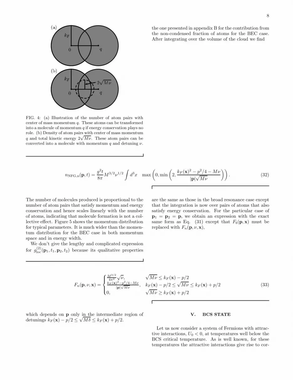
FIG. 4: (a) Illustration of the number of atom pairs withcenter of mass momentum q. These atoms can be transformedinto a molecule of momentum q if energy conservation plays norole. (b) Density of atom pairs with center of mass momentum

q and total kinetic energy 2√

Mν. These atom pairs can beconverted into a molecule with momentum q and detuning ν.

the one presented in appendix B for the contribution fromthe non-condensed fraction of atoms for the BEC case.After integrating over the volume of the cloud we find

nNFG,n(p, t) =g2t

8πM3/2ν1/2

∫

d3x max

(

0,min

(

2,kF (x)2 − p2/4 −Mν

|p|√Mν

))

. (32)

The number of molecules produced is proportional to thenumber of atom pairs that satisfy momentum and energyconservation and hence scales linearly with the numberof atoms, indicating that molecule formation is not a col-lective effect. Figure 5 shows the momentum distributionfor typical parameters. It is much wider than the momen-tum distribution for the BEC case in both momentumspace and in energy width.

We don’t give the lengthy and complicated expression

for g(2)loc(p1, t1,p2, t2) because its qualitative properties

are the same as those in the broad resonance case exceptthat the integration is now over pairs of atoms that alsosatisfy energy conservation. For the particular case ofp1 = p2 = p, we obtain an expression with the exactsame form as Eq. (31) except that Fb(p,x) must bereplaced with Fn(p, ν,x),

Fn(p, ν,x) =

M3/2

4π2

√ν,

√Mν ≤ kF (x) − p/2

kF (x)2−p2/4−Mν

|p|√

Mν, kF (x) − p/2 ≤

√Mν ≤ kF (x) + p/2

0,√Mν ≥ kF (x) + p/2

(33)

which depends on p only in the intermediate region ofdetunings kF (x) − p/2 ≤

√Mδ ≤ kF (x) + p/2.

V. BCS STATE

Let us now consider a system of Fermions with attrac-tive interactions, U0 < 0, at temperatures well below theBCS critical temperature. As is well known, for thesetemperatures the attractive interactions give rise to cor-

9

0

0.5

1

1.5

20

0.51

1.52

0

0.5

1

ν/µ0p/k

F(0)

n NF

G,n

(p,t)

[a.u

.]

FIG. 5: Momentum distribution of molecules produced from anormal Fermi gas in the narrow resonance limit for g = 10−3µ.

relations between pairs of atoms in time reversed statesknown as Cooper pairs. We assume that the sphericallysymmetric trapping potential is sufficiently slowly vary-ing that the gas can be treated in the local density ap-proximation. More quantitatively, the local density ap-proximation is valid if the size of the Cooper pairs, givenby the correlation length

λ(r) = vF (r)/π∆(r),

is much smaller than the oscillator length for the trap.Here, vF (r) is the velocity of atoms at the Fermi surfaceand ∆(r) is the pairing field at distance r from the origin,which we take at the center of the trap.

Before turning to the coupled atom-molecule systemwe outline our treatment of the atomic system. Weclosely follow the approach of Houbiers et. al. [41]. Weassume that locally at each r, the wave function can beapproximated by the BCS wave function for a homoge-nous gas,

|BCS(r)〉 =∏

k

(uk(r) + vk(r)c†−k,↑c†k,↓)|0〉, (34)

with Bogoliubov amplitudes

u2k(r) =

1

2

(

1 +ξk(r)

√

∆2(r) + ξ2k(r)

)

, (35)

v2k(r) =

1

2

(

1 − ξk(r)√

∆2(r) + ξ2k(r)

)

. (36)

Here ξk(r) = ǫk−µloc(r) is the kinetic energy of an atommeasured from the local chemical potential defined as

µloc(r) = µ0 − U(r) − U0n(r). (37)

In contrast to the normal Fermi gas, we have includeda Hartree-Fock mean-field energy to the local chemicalpotential since we can no longer ignore the effect of thetwo-body interactions in the gas. To an excellent approx-imation we can use the relation Eq. (26) between densityand local chemical potential. Then, for a given numberof atoms N , Eq. (37) is an implicit equation for µ0. Wesolve it numerically and hence determine the density pro-file n(r) and the local chemical potential µloc(r).

The gap parameter ∆(r) = U0/2V∑

k uk(r)vk(r) isdetermined by the gap equation

−π2kF (0)a

= µ0k−3F (0)

∫ ∞

0

dkk2

(

1√

ξ2k(r) + ∆2(r)− 1

ξk(r)

)

,

(38)where the ultra-violet divergence has been removed byrenormalizing the bare background scattering strengthto the two-body T-matrix using the Lippmann-Schwingerequation (see ref. [41]). We solve the gap equation nu-merically using the previously determined local chemicalµloc.

A. Broad resonance, Ekin ≪ g√

N

We find the momentum distribution of the moleculesfrom the BCS type state by repeating the calculationdone in the case of a normal Fermi gas. For the BCS wavefunction, the relevant atomic expectation values factorizeas

⟨

c†p/2−k1,↑c

†p/2+k1,↓cp/2+k2,↑cp/2−k2,↓

⟩

=⟨

c†p/2−k1,↑c

†p/2+k1,↓

⟩⟨

cp/2+k2,↓cp/2−k2,↑⟩

+⟨

c†p/2−k1,↑cp/2+k2,↓

⟩⟨

c†p/2+k1,↓cp/2−k2,↑

⟩

(39)

10

and the momentum distribution of the molecules be-comes

nBCS,b(p, t) = (gt)2

∣

∣

∣

∣

∣

∑

k

⟨

cp/2+k,↓cp/2−k,↑⟩

∣

∣

∣

∣

∣

2

+∑

k

⟨

c†p/2−k,↑cp/2+k,↓

⟩⟨

c†p/2+k,↓cp/2−k,↑

⟩

≈ (gt)2

∣

∣

∣

∣

∣

∑

k

⟨

cp/2+k,↓cp/2−k,↑⟩

∣

∣

∣

∣

∣

2

+ nNFG,b(p, t). (40)

In going from the first to the second line we have as-sumed that the interactions are weak enough so that themomentum distribution of the atoms is essentially thatof a two component Fermi gas. This is justified becausethe Cooper pairing only affects the momentum distribu-tion in a small shell of thickness 1/λ(r) ≪ kF (r) aroundthe Fermi surface.

The first term involves the square of the pairing field.It is proportional to the square of the number of pairedatoms which, below the critical temperature, is a finitefraction of the total number of atoms. This quadraticdependence indicates that it is the result of a collectiveeffect. This term can be related to the two-point corre-lation function in position space as

⟨

cp/2+k,↓cp/2−k,↑⟩

=

∫

d3xd3r

Ve−ip·x−ik·r〈ψ↓(x − r/2)ψ↑(x + r/2)〉 (41)

where ψ↑,↓ are the atomic field operators in positionspace. In the local density approximation, the correla-tion function varies with x on a length scale RTF. Onthe other hand, the expectation value in the integral fallsoff to zero for r > λ(r) and we can therefore treat thecorrelation function as being independent of x when per-forming the integration over r,

⟨

cp/2+k,↓cp/2−k,↑⟩

=

∫

d3x

Ve−ip·x〈ck,↓c−k↑〉

∣

∣

∣

x(42)

The expectation value on the right hand side is evalu-ated using the local density approximation at position x.Inserting the result into Eq. (40) and making use of thegap equation we find

nBCS,b(p, t) = (gt)2

[

∣

∣

∣

∣

∫

d3xe−ix·p(

1 − 2aΛ

π

)

2∆(x)

U0

∣

∣

∣

∣

2

+ nNFG,b(p, t)

]

. (43)

Following ref. [41] we have replaced the bare backgroundcoupling strength by

U0 = U01

1 − 2aΛπ

, (44)

where Λ is a momentum cut-off and is of the order of theinverse of the range of the inter-atomic potential.

Using the numerically determined ∆(x) we can read-ily perform the remaining Fourier transform in Eq. (43).The result of such a calculation is shown in Fig. 1. Sincethe gap parameter changes over distances of order RTF

the contribution from the pairing field has a typical widthof order 1/RTF . This is very similar to the BEC case.The background from the unpaired atoms on the otherhand has a typical width kF (0) = (3π2n0)

1/3 which is

11

similar to the width of the noise contribution in the BECcase, see inset in Fig. 1. This similarity can be under-stood by recalling that for a weakly interacting conden-

sate, n1/30 a = β ≪ 1, which when substituted into the

definition of the healing length gives 1/ξ = (8πβ)1/2n1/30 .

For typical β ∼ 0.1, this is comparable to kF (0) for equaldensities.

Because of the collective nature of the coherent con-tribution it will dominate over the background, nNFG,b,for strong enough interactions and large enough particlenumbers. The narrow width and the collective enhance-ment of the molecule production are the reasons why themomentum distribution of the molecules is such an excel-lent indicator of the presence of a superfluid componentand the off-diagonal long range order accompanying it.

For weak interactions such that the coherent contribu-tion is small compared to the incoherent contribution, thesecond order correlations are close to those of a normalFermi gas given by Eq. (31), g(2)(p,x, t) ≈ 2. However,in the strongly interacting regime, kF |a| ∼ 1, and largeN , the coherent contribution from the paired atoms dom-

inates over the incoherent contribution from unpairedatoms. In this limit one finds that the second-order cor-relation is close to that of the BEC, g(2)(p,x, t) ≈ 1. Thephysical reason for this is that at the level of evenordercorrelations the pairing field behaves just like the meanfield of the condensate. This is clear from the factor-ization property of the atomic correlation functions, Eq.(39), in terms of the normal component of the densityand the anomalous density contribution due to the meanfield. In this case, the leading order terms in N are givenby the anomalous averages. In the strongly interactinglimit, the contribution from the ‘unpaired’ atoms is verysimilar in nature to the contribution from the fluctua-tions in the BEC case.

B. Narrow resonance, Ekin ≫ g√

N

A calculation similar to the one presented in AppendixB for the BEC case leads to

nBCS,n(p, t) =

∣

∣

∣

∣

∣

∑

k

∆(ν − k2/M)〈cp/2+k,↓cp/2−k,↑〉∣

∣

∣

∣

∣

2

+ nNFG,n(p, t), (45)

where we have assumed again that the gas is weakly in-teracting. Inserting Eq. (19) for ∆ in the limit νt → ∞

and performing similar manipulations as in the broadresonance case leads to

nBCS,n(p, t) =g2M3

π2p2

∣

∣

∣

∣

∣

∫ ∞

0

dω√ω

(

πδ(ν − ω) + iP1

ν − ω

)

∫ RTF

0

drr sin(pr)〈c√Mω,↓c−√

Mω,↑〉∣

∣

∣

r

∣

∣

∣

∣

∣

2

+ nNFG,n (46)

where again the pairing field 〈ck,↓c−k,↑〉|r = uk(r)vk(r)can be evaluated using the local density approximation.Figure 6 shows an example of the pairing field across thetrap. Two qualitatively different cases have to be distin-guished depending on the strength of the interactions.

If the interactions are fairly strong so that the pair-ing field, uk(r)vk(r), is nonzero in a rather wide regionaround kF (r), the pairing field will be a slowly varyingfunction across the atomic cloud. Then the remainingintegral in eq. (46) can be easily evaluated numericallyand we find a momentum distribution of the moleculeswhich is similar to the BEC case. This limit is illustrated

in fig. 7. The width of the momentum distribution ofthe molecules is again of order 1/RTF . It is known thatin the strongly interacting limit, the size of the Cooperpairs becomes comparable to the interparticle spacing,λ(r) ∼ 1/kF (r). The Cooper pairs are no longer delo-calized across the extent of the cloud but now approachthe limit of localized bosonic ”quasi-molecules”. Thusit is not surprising that the momentum distribution ofmolecules formed from a BCS type state approaches theone we found in the BEC case.

On the other hand, if the interactions between theatoms are weak the pairing field is a very narrow func-

12

10 30 500

0.5

1

1.5

r [1/kF(0)]

kF(r)→

k [k

F(0

)]

FIG. 6: Pairing field 〈ck,↓c−k,↑〉 = ukvk across the trap forkF a = 0.5 and aosc = 5k−1

F (0). The black solid line indicatesthe local Fermi momentum kF (r).

tion of momentum and hence, for fixed momentum, alsoof position as can be seen from Fig. 6. Then the integralin Eq. (46) has contributions from a rather narrow re-gion in space only and the momentum distribution willaccordingly become wider and smaller.

Probing the BCS system in the narrow resonanceregime also yields spatial information about the atomicstate. By tuning ν = 2µloc(r) the molecular signal ismost sensitive to the pairing field near r and less sensi-tive to other regions in the trap.

A qualitative difference between the BCS and BECcases becomes apparent if one looks at the number ofmolecules as a function of the detuning. While we findthat there is only a very narrow distribution of detunings

with width ∼ (2π/RTF )2

2M that leads to molecule formationin the BEC case, molecules are being formed for detun-ings well below ν ∼ 2µ0. The non-homogeneity of thetrapped atom system manifests itself in a completely dif-ferent way in the two cases. In the BEC case, the totalenergy of a particle in the condensate is just the chemi-cal potential while the kinetic energy of a particle is verysmall compared to the mean field energy in the ThomasFermi limit. Upon release, the atoms in the condensateall have a spread in kinetic energies that is of the or-

der (2π/RT F )2

2M due entirely to zero point motion. On theother hand, in the BCS case the superfluid forms at eachposition near the local Fermi momentum. Hence, atomsin the BCS state have a large energy spread that is oforder ∼ µ0 with the kinetic energies of the paired atomsbeing centered around µloc(r) with a width ∆(r).

For the second order moment, g(2)(p,x, t), the samegeneral arguments that were put forward in the discus-sion of the broad resonance also apply to the narrow res-onance. In the strongly interacting limit, the molecularfield is again approximately coherent with a noise contri-bution from the unpaired fermions.

FIG. 7: Momentum distribution of molecules formed from astrong coupling (kF a = 0.5) BCS system in the narrow reso-nance regime as a function of detuning ν for aosc = 5k−1

F (0).Well below ν = 2µ the figure is a bit noisy because the Fouriertransform in eq. (46) gets its main contribution from a verynarrow region in space where the solution of the gap equationis numerically challenging.

VI. SUMMARY

We examined the momentum distribution and momen-tum correlations of molecules formed by a Feshbach reso-nance or by photoassociation from a quantum degenerateatomic gas. Our study elucidated the effect of the atomictrapping potential as well as the strength of the atom-molecule coupling relative to the characteristic energiesof the atoms on the molecular momentum distribution.

Molecules produced from an atomic BEC show a rathernarrow momentum distribution that is comparable to thezero-point momentum width of the atomic BEC fromwhich they are formed. In the case of a narrow reso-nance, energy conservation limits the molecules to onlya narrow energy range. The molecule production is acollective effect with contributions from all atom pairsadding up constructively, as indicated by the quadraticscaling of the number of molecules with the number ofatoms. Each mode of the resulting molecular field is toa very good approximation coherent (up to terms of or-der O(1/N)). The effects of noise, both due to finitetemperatures and to vacuum fluctuations, are of relativeorder O(1/N). They slightly increase the g(2) and causethe molecular field in each momentum state to be onlypartially coherent.

In contrast, the momentum distribution of moleculesformed from a normal Fermi gas is much broader witha typical width given by the Fermi momentum of theinitial atomic cloud. The molecule production is not col-lective as the number of molecules only scales like thenumber of atoms rather than the square. In this case,the second-order correlations of the molecules exhibitsuper-Poissonian fluctuations, and it was argued that themolecules are well characterized by a thermal field.

13

The case where molecules are produced from pairedatoms in a BCS-like state shares many properties withthe BEC case: The molecule formation rate is collective,their momentum distribution is very narrow in compar-ison to the normal Fermi gas, and the molecular fieldis essentially coherent. The non-collective contributionfrom unpaired atoms has a momentum distribution verysimilar to that of the quasiparticle fluctuations in theBEC case.

In a future publication we will use the Bogoliubov-de-Gennes equations to describe the BCS type state whichis again probed with a molecular field. Thus we will beable to go beyond the local density approximation andwe can study the BEC-BCS cross-over regime. Also, thiswill allow us to study the validity of the local densityapproximation more carefully.

This work is supported in part by the US Office ofNaval Research, by the National Science Foundation, bythe US Army Research Office, and by the National Aero-nautics and Space Administration.

APPENDIX A: CALCULATION OF n(p) FOR

g ≫ Ekin FOR A BEC

In this appendix we show how the decomposition of theatomic field operator into condensed and non-condensedfraction together with the local density approximationfor the non-condensed part can be used to calculate themomentum distribution of the molecules for the case ofan initial BEC of atoms. More details on the propertiesof fluctuations at non-zero temperatures and the use ofthe local density approximation for their description can

be found in references [37, 38, 39].

The starting point of our calculation is eq. (6) for themomentum distribution of the molecules. It reduces theproblem to evaluating an integral over expectation valuesin the undisturbed atomic field at t = 0. The relevantexpectation values are most transparently calculated bypartitioning the quantization volume V into smaller vol-umes Vj that are larger than the coherence length ξ. Par-titioning the atomic field operator accordingly, we get

ψ(x) =∑

j

Aj(x)χ0(x)c+∑

j

δψ(j)loc(x), (A1)

where we have introduced functions Aj(x) that are

one in volume Vj and zero otherwise, and δψ(j)loc(x) =

Aj(x)δψ(x). The partitioning of the field operator is il-lustrated in fig. 8. We go over to the Fourier transform

cp =

∫

d3x√Ve−ipxψ(x) = χ0(p)c+

∑

Vj

√

Vj

Vδc(j)p (A2)

where δc(j)(p) is the annihilation operator for a fluctua-tion of momentum p in volume Vj . In the local densityapproximation, fluctuations in different cells Vj are un-correlated and we have

〈δc(i)k1

†δc

(j)k2

〉 ≡ δi,jδk1,k2〈δc(i)k1

†δc

(i)k1〉. (A3)

Inserting in eq. (6), keeping only terms of first order inthe fluctuations and making use of relation (A3) we find

nBEC,b(p, t) = (gt)2N(N − 1)∑

k1,k2

χ∗0(p/2 − k1)χ

∗0(p/2 + k1)χ0(p/2 − k2)χ0(p/2 + k2)

+ 4(gt)2N∑

k,j

Vj

V|χ0(p − k)|2〈c(j)†k c

(j)k 〉. (A4)

The coherent term is readily brought to the form givenin eq. (7). In the incoherent term we notice that |χ0(p)|2is a much narrower function than 〈c(j)†k c

(j)k 〉, the former

having a typical width of ∼ 1/RTF while the latter has atypical width of ∼ 1/ξ. Hence, to a good approximation,

〈c(j)†k c(j)k 〉 can be treated as a constant for the momentum

range for which |χ0(p)|2 is nonzero and we obtain

4(gt)2N∑

k,j

Vj

V|χ0(p− k)|2〈c(j)†k c

(j)k 〉

≈ 4(gt)2N∑

j

Vj

V〈c(j)†k c

(j)k 〉

∑

k

|χ0(p − k)|2

= 4(gt)2N∑

j

Vj

V〈c(j)†k c

(j)k 〉, (A5)

where we have made use of the normalization of χ0(x)in the last step. Since ξ ≪ RTF the volumes Vj canbe made small and the sum can be approximated by an

14

1

x

�

0

(x)

^

(x)

V

j

(x)V

j�1

(x) V

j+1

(x)

A

j

(x)

FIG. 8: Illustration of the partitioning of quantization vol-ume and atomic field operator. Also indicated is the functionAj(x).

integral, leading to eq. (7).

APPENDIX B: CALCULATION OF n(p) FOR

g ≪ Ekin FOR A BEC

The calculation goes along similar lines as in the broadresonance case but the evaluation of the integrals is morecomplicated. Repeating the calculation of the broad res-onance case that lead to eq. (A4) with ap now replacedaccording to eq. (18) we find, again to first order in thefluctuations

nBEC,n(p, t) = N(N − 1)∣

∣

∣

∑

k

∆(Ep − ǫp/2+k − ǫp/2−k, t)χ0(p/2 + k)χ0(p/2 − k)∣

∣

∣

2

+ 4N∑

k,j

Vj

V

∣

∣∆(Ep − ǫp/2+k − ǫp/2−k, t)∣

∣

2 |χ0(p − k)|2〈c(j)†k c(j)k 〉

≡ ncoh(p, t) + nincoh(p, t). (B1)

Let us first consider the coherent part ncoh(p, t). Goingover from the summation to an integral in the usual way,

making the substitution ω = k2/M and introducing polarcoordinates we find

ncoh(p, t) =VM3/2

π223

∫ ∞

0

dω∆(ν − ω, t)

∫ π

0

dϑ sinϑ

×√ωχ0

(√

p2/4 +Mω + |p|√Mω cosϑ

)

χ0

(√

p2/4 +Mω − |p|√Mω cosϑ

)

(B2)

In the limit t→ ∞, ∆(ν − ω) becomes [42],

limt→∞

∆(ν − ω, t) = g

(

πδ(ν − ω) − iP1

ν − ω

)

(B3)

where, as usual, P means that the integral has to be takenin the sense of the Cauchy-principal value. The real part

can be evaluated by making use of the δ-function and forthe imaginary part we have to rely on numerical methodsto calculate the principal value integral.

Making similar manipulations of the sums over mo-menta for the incoherent part leads to

nincoh(p, t) = 4NM3/2

8π2

∑

j

Vj

∫ π

0

dϑ sinϑ

×∫ ∞

0

dω√ω|∆(ν − ω, t)|2

∣

∣

∣χ0

(√

p2/4 +Mω − |p|√Mω cosϑ

)

∣

∣

∣

2

〈c(j)†√Mω

c(j)√

Mω〉. (B4)

15

Using the delta function

limt→∞

|∆(ν − ω)|2 = πg2tδ(ν − ω). (B5)

to perform the integral in the limit as t goes to inifinitywe arrive at eq. (20).

[1] S. Inouye et al., Nature (London) 392, 151 (1998).[2] E. Timmermans, P. Tommasini, M. Hussein, and A. Ker-

man, Phys. Rep. 315, 199 (1999).[3] P. O. Fedichev, Yu Kagan, G. V. Shlyapnikov, and J. T.

M. Walraven, Phys. Rev. Lett. 77, 2913 (1996).[4] M. Theis, G. Thalhammer, K. Winkler, M. Hellwig,

G. Ruff, R. Grimm, and J. H. Denschlag, Phys. Rev.Lett. 93, 123001 (2004).

[5] R. Wynar et al., Science 287, 1016 (2000).[6] E. A. Donley, N. R. Claussen, S. T. Thompson, and C. E.

Wieman, Nature (London) 417, 529 (2002).[7] S. Durr, T. Volz, A. Marte, and G. Rempe, Phys. Rev.

Lett. 92, 020406 (2004).[8] M. Greiner, C. A. Regal, and D. S. Jin, Nature (London)

426, 537 (2003).[9] M. W. Zwierlein et al., Phys. Rev. Lett. 91, 250401

(2003).[10] S. Jochim et al., Science 301, 2101 (2003).[11] M. Greiner, O. Mandel, T. Esslinger, T. W. Hansch, and

I. Bloch, Nature 415, 39 (2002).[12] M. Greiner, O. Mandel, T. W. Hansch, and I. Bloch,

Nature 419, 51 (2002).[13] D. Jaksch, C. Bruder, J. I. Cirac, C. W. Gardiner, and

P. Zoller, Phys. Rev. Lett. 81, 3108 (1998).[14] H. T. C. Stoof (International school of physics ‘Enrico

Fermi’, Varenna, 1998).[15] E. Timmermans, Physica Scripta T110, 302 (2004).[16] E. Timmermans, K. Furuya, P. W. Milonni, and A. K.

Kerman, Phys. Lett. A 285, 288 (2001).[17] C. A. Regal, M. Greiner, and D. S. Jin, Phys. Rev. Lett.

92, 040403 (2004).[18] M. Bartenstein et al., Phys. Rev. Lett. 92, 120401 (2004).[19] M. Zwierlein et al., Phys. Rev. Lett. 92, 120403 (2004).[20] H. T. C. Stoof, M. Houbiers, C. A. Sackett, and R. G.

Hulet, Phys. Rev. Lett. 76, 10 (1996).[21] G. Bruun, Y. Castin, R. Dum, and K. Burnett, Eur.

Phys. J. D 7, 433 (1999).[22] C. Chin, M. Bartenstein, A. Altmeyer, S. Riedl,

S. Jochim, J. Hecker Denschlag, and R. Grimm, Science305, 1128 (2004).

[23] J. Kinast, S. L. Hemmer, M. E. Gehm, A. Turlapov, andJ. E. Thomas, Phys. Rev. Lett. 92, 150402 (2004).

[24] M. Bartenstein, A. Altmeyer, S. Riedl, S. Jochim,C. Chin, J. H. Denschlag, and R. Grimm, Phys. Rev.

Lett. 92, 203201 (2004).[25] E. A. Burt, R. W. Ghrist, C. J. Myatt, M. J. Holland,

E. A. Cornell, and C. E. Wieman, Phys. Rev. Lett. 79,337 (1997).

[26] D. Hellweg, L. Cacciapuoti, M. Kottke, T. Schulte,K. Sengstock, W. Ertmer, and J. J. Arlt, Phys. Rev.Lett. 91, 010406 (2003).

[27] L. Cacciapuoti, D. Hellweg, M. Kottke, T. Schulte,W. Ertmer, J. J. Arlt, K. Sengstock, and L. Santos, Phys.Rev. A 68, 053612 (2003).

[28] E. Altman, E. Demler, and M. D. Lukin, Phys. Rev. A70, 013603 (2004).

[29] R. Bach and K. Rzazewski, Phys. Rev. Lett. 92, 200401(2004).

[30] R. J. Glauber, Phys. Rev. 130, 2529 (1963).[31] R. J. Glauber, Phys. Rev. 131, 2766 (1963).[32] M. Naraschewski and R. J. Glauber, Phys. Rev. A 59,

4595 (1999).[33] K. E. Cahill and R. J. Glauber, Phys. Rev. A 59, 1538

(1999).[34] D. Meiser and P. Meystre (2004), cond-mat/0410349.[35] M. Holland, S. J. J. M. F. Kokkelmans, M. L. Chiofalo,

and R. Walser, Phys. Rev. Lett. 87, 120406 (2001).[36] M. L. Chiofalo, S. J. J. M. F. Kokkelmans, J. N. Milstein,

and M. J. Holland, Phys. Rev. Lett. 88, 090402 (2002).[37] D. A. W. Hutchinson, E. Zaremba, and A. Griffin, Phys.

Rev. Lett. 78, 1842 (1997).[38] J. Reidl, A. Csordas, R. Graham, and P. Szepfalusy,

Phys. Rev. A 59, 3816 (1999).[39] T. Bergeman, D. L. Feder, N. L. Balazs, and B. I. Schnei-

der, Phys. Rev. A 61, 063605 (2000).[40] D. A. Butts and D. S. Rokhsar, Phys. Rev. A 55, 4346

(1997).[41] M. Houbiers et al., Phys. Rev. A 56, 4864 (1997).[42] E. Merzbacher, Quantum Mechanics (John Wiley &

Sons, New York, 1998), 3rd ed.[43] We denote the function in Eq. (19) by ∆ because it has

properties similar to the usual δ-function. Confusion withthe local gap parameter introduced below, which we alsodenote by ∆, cannot arise because the first always hasenergies as its argument while the latter has positions asits argument.