Monetary transmission in Germany: Lessons for the euro area

Kirstin Hubrich, Peter Vlaar12

November, 2000

ABSTRACT

This study analyses the transmission of monetary policy in Germany for the EMS period in the frame-

work of a structural vector error correction model (S-VECM). Three stable cointegration relationships

are found: a money demand relation, an interest rate spread and a stationary real interest rate. Based

on both contemporaneous and long-run restrictions, five structural shocks to the economy are identified.

In contrast to analyses for the euro area, we find that output and inflation are not independent in the

long run for Germany. In accordance with results previously found for Europe, we do not find strong

support for monetary targeting for Germany. Our analysis indicates that uncertainties remain concerning

the controllability of money and its usefulness as a leading indicator with respect to inflation. Stability

of the money demand relationship does not seem to be problematic.

Keywords: Monetary transmission, Germany, generalised common trends model

JEL Classification System-Numbers: C32, C52, E41, E43, E52

1 e-mail: k.s.e.m.hubrich@dnb.nl, p.j.g.vlaar@dnb.nl; address: De Nederlandsche Bank, Econometric Researchand Special Studies Department, P.O.Box 98, 1000 AB Amsterdam, The Netherlands, http://www.dnb.nl

2 This paper has been circulated under the title ‘Germany and the euro area: Differences in the transmissionprocess of monetary policy’. We would like to thank Jörg Breitung, Bertrand Candelon, Peter van Els, CarstenFolkertsma, Helmut Lütkepohl, Dieter Nautz, Hans-Eggert Reimers, Nikolaus Siegfried and Jürgen Wolters aswell as participants of the 8th World Congress of the Econometric Society in Seattle and the Annual Meeting ofthe Verein für Socialpolitik in Berlin for helpful comments on earlier versions of the paper. The views expressed inthis paper do not necessarily reflect those of De Nederlandsche Bank.

– 4 –

– 5 –

1 INTRODUCTION

Recently a number of studies have analysed the transmission process of monetary policy in Europe

based on aggregated euro area data. However, conclusions for the monetary policy of the European

Central Bank (ECB) drawn from past experience on the basis of the aggregated European level have to

be considered with some caution. The fact that most euro members started from a situation of relatively

high inflation and did not follow an independent monetary policy during the period of investigation

might have a significant impact on the effectiveness of monetary policy. As this environment of high but

converging inflation is not likely to be representative for the Economic and Monetary Union in Europe

(EMU) it is useful to investigate the German experience as well. This provides a second benchmark –

the first being based on aggregated euro area data – against which monetary transmission mechanisms in

EMU can be evaluated.

Regarding the monetary policy of the ECB the German experience is indeed most relevant for at least

three reasons. First, the Deutsche Bundesbank (henceforth: Bundesbank) was the leading monetary au-

thority in the European Monetary System following a successful independent monetary policy, focussing

solely on price stability with a prominent role for money as an intermediate target. Second, as a conse-

quence German inflation was never very high – a situation likely to be representative for EMU. Third, in

order to inherit the reputation of the Bundesbank and to cope with the uncertainties of the starting period

of EMU, the ECB has chosen a policy very similar to the one of the Bundesbank. Notwithstanding these

similarities, differences in monetary transmission between Germany and the euro area could of course

also be due to typical German circumstances that might not be representative for EMU. Since Germany

is the largest economy in the EMU area however, the analysis would still provide highly relevant insights

for the ECB’s monetary policy.

The aim of this study is to analyse whether the transmission of monetary policy in the euro area re-

sembles features of the monetary transmission process in Germany. The outcome of this analysis also

contributes to the discussion whether the ECB should follow a monetary policy strategy where money

plays a prominent role.

It is important for the analysis of the transmission process of monetary policy to take long-run relations

between fundamental macroeconomic variables in an economy as well as short-run dynamics into ac-

count. Therefore, the analysis presented here extends the multivariate approach applied to a German

macroeconomic system in Hubrich (1999, 2001) employing the long-run relationships analysed there,

that is a money demand relation, a Fisher relation as well as an interest rate spread, as a basis for mod-

elling a dynamic cointegrated system for Germany. For this purpose the structural vector error correction

– 6 –

model (S-VECM) approach suggested by Vlaar (1998), that incorporates restrictions on the cointegra-

tion vectors, will be applied to analyse the transmission of shocks in the economy. The results from the

analysis of the transmission of monetary policy in Germany will be compared with analyses on the basis

of aggregated European data prior to EMU, especially with Vlaar and Schuberth (1999) and Coenen and

Vega (1999).

The paper is structured as follows: In the next section, the insights and problems of studies based on

aggregated euro area data in contrast to cross-national comparisons are discussed. In the third section,

recent literature on the German transmission of monetary policy is reviewed. The fourth section presents

a discussion of some methodological issues. The initial system as well as the cointegration analysis are

presented in the fifth section. Section six displays the analysis of the transmission of monetary policy

within a structural vector autoregressive (SVAR) framework and section seven focuses on the comparison

between Germany and aggregated euro area results. Section eight presents the main conclusions.

– 7 –

2 AGGREGATED EURO AREA VERSUS NATIONAL EVIDENCE

The discussion concerning the introduction of a common European currency has initiated empirical stud-

ies based on aggregated European data, e.g. studies on money demand on the European level as Monti-

celli and Papi (1996), Wesche (1997), Fagan and Henry (1998) and Fase and Winder (1998). Recently,

Vlaar and Schuberth (1999), Monticelli and Tristani (1999) and Coenen and Vega (1999) have presented

SVAR studies analysing the transmission of monetary policy for different sets of variables based on

aggregated data.

Several problems arise with respect to policy conclusions for EMU drawn from such an analysis. The

structural break due to EMU might affect the monetary transmission mechanism in several EMU coun-

tries. For Germany this structural break is likely to be less important as the policy of the ECB is similar

to that of the Bundesbank and the low inflation environment is also likely to be representative for EMU.

Moreover, as Germany is the largest country in the euro area, the German experience can provide a

valuable benchmark against which monetary transmission mechanisms in EMU can be evaluated.

Apart from the possibility of a structural break, information on the transmission channels of monetary

policy in individual countries of the euro area is relevant in itself for the monetary policy decisions of

the ECB. Although the ECB has to consider the euro area as a whole, knowledge on the differences in

monetary transmission facilitates the evaluation of costs and benefits of policy actions at times when

different countries require different policies.

A more technical concern is that the analysis of aggregated data implies possibly invalid restrictions on

the coefficients implicit in the aggregation of data across different countries.1 Although the specification

bias of national estimations due to the omission of relevant euro area foreign variables is avoided by

aggregated analysis (see e.g. Monticelli and Papi, 1996; Pesaran, Pierse and Kumar, 1989), a bias due

to differences in parameters or even functional form between national specifications is likely. This is a

further argument that national and aggregated analyses should be considered complementary.

One approach to analyse the national differences in the transmission of monetary policy has been pre-

sented by Fase and Winder (1993) who compare national money demand relations across European

countries. They find lower sensitivity of money demand to interest rate and inflation changes in the

southern than in the northern EC countries. Furthermore, they find differences in the stability of the

demand for money, specifically that German money demand is more stable than the demand for money

in other countries. Wesche (1997), analysing an aggregated money demand relation for different sets of

1 For a presentation of these problems within the framework of a two-country model, see Monticelli and Tristani(1999).

– 8 –

European countries, finds a stable aggregated money demand function for a group of countries including

Germany, but instability is indicated if Germany is excluded from the aggregated data. She concludes

that the aggregated European relation reflects the stability of German money demand.

These analyses indicate the importance of national differences in the context of the monetary policy of

the ECB. The present paper extends such a comparison to other aspects of the transmission of monetary

policy by comparing the monetary transmission between Germany and the aggregated euro area. In such

an analysis other important aspects of monetary transmissions, such as controllability of money and a

causal link between money growth and future inflation can also be considered.

Monticelli and Tristani (1999) consider monetary transmission in a small system of three variables and

compare some of their empirical results based on aggregated data with the cross-country study by Gerlach

and Smets (1995) based on the same set of variables and the same identification scheme. Comparing the

effect of some of the shocks between single countries and the euro area provides mixed results, i.e. some

shocks differ whereas some do not.

There are two studies that consider the transmission of monetary policy on an aggregated euro area level

using the S-VECM approach. The first study is Vlaar and Schuberth (1999), henceforth VS, who analyse

a six variable system including wealth besides real money, real output, the inflation rate and long- as well

as short-term interest rates. The authors find two cointegration relations, a money demand relation and a

stationary real long-term interest rate, but a stationary interest rate spread is rejected in their system. They

identify six different shocks affecting the euro area economy. Regarding the monetary policy strategy

the effect of a positive shock in the interest rate is of relevance. Since this monetary policy shock leads

to an increase in nominal money, VS conclude that money is difficult to control on a European level.

In contrast, Coenen and Vega (1999), henceforth CV, consider a five variable system not including wealth,

also employing the same S-VECM methodology. They find three stable long-run relationships. In addi-

tion to the money demand relation and the stationary real interest rate they also find a stationary spread

between short- and long-term interest rates. CV identify five shocks affecting the euro area economy.

They impose that real money balances are in the long run not affected by a monetary policy shock. Con-

sequently, controllability of money is not a problem in the long run because the temporary fall in the

inflation rate due to the interest rate rise decreases the price level permanently. However, their results

indicate that short-term controllability is problematic.

Regarding the causal link between money growth and inflation, neither VS nor CV find convincing

evidence for a leading indicator role of money growth on inflation. Most increases in inflation are not

preceded by an increase in money growth. The reverse causality is very prominent though.

– 9 –

3 THE TRANSMISSION PROCESS IN GERMANY: RECENT LITERATURE

Since the Bundesbank followed a monetary targeting strategy since 1975, lots of emphasis in the em-

pirical studies has been on analysing whether the preconditions of monetary targeting were fulfilled in

Germany. In this context, the stability of the demand for money, the controllability of the monetary

aggregate by the central bank’s monetary policy actions and the question whether a causal link between

money and inflation, i.e. between the intermediate and final target, exists, are of interest.

Especially after German reunification the question has been raised whether the Bundesbank’s strategy of

monetary targeting was still appropriate since the stability of the demand for money might be impaired.

A number of single-equation studies, for example Issing and Tödter (1995) and Wolters, Teräsvirta and

Lütkepohl (1998), among others, indicated that German money demand is still stable if German reunifi-

cation is modelled including dummy variables.

The analyses of a German monetary system presented by Juselius (1996, 1998), Hubrich (1999, 2001),

Lütkepohl and Wolters (1998) and Beyer (1998) have also shown that the structural break embodied

by German reunification can be modelled by dummy variables. Covering different sample periods and

seasonally unadjusted as well as seasonally adjusted data, these studies, except for Juselius (1996, 1998),

find a stable German money demand relation.

Juselius (1996, 1998) finds a structural break in 1983 and she concludes that this break marks the liber-

alisation of capital markets in Europe. However, the fact that capital markets in Germany have largely

been liberalised at the beginning of the 1970s (see also Issing, 1997), raises doubts about the plausibility

of this finding.

Besides studying the stability of money demand, some of the systems analyses cited above have also

tested and found stationarity of the spread between short-and long-term interest rates as well as the real

interest rate, both relevant for the transmission of monetary policy into the economy and its predictability.

The stability of these long-run relationships will also be analysed in this study and will be taken into

account with respect to the transmission of monetary policy in Germany.

In addition to the stability of the demand for M3 further conditions have to be fulfilled, for a monetary

targeting strategy to work. Therefore, the controllability of the monetary aggregate by the central bank

has been analysed by Cabos, Funke and Siegfried (1999). Employing Markov-Switching Models they

analyse the link between monetary policy actions and inflation and find that control problems with respect

to money are slightly higher in a monetary targeting strategy than in an inflation targeting regime.

– 10 –

The causal link between money and prices is one main focus of the analysis by Lütkepohl and Wolters

(1998). On the basis of a system taking a long-run money demand equation derived in a single-equation

procedure into account, an impulse response analysis to investigate dynamic interdependencies between

the variables as well as the transmission mechanism is carried out. They find no strong influence of

money growth on inflation, but considerable effects of shocks in the inflation rate on money growth.

This result of the study allows some doubt about the strength of the causal link between money growth

and inflation that is a precondition for a strategy of monetary targeting.2

Clarida and Gertler (1996) and Bernanke and Mihov (1997) have presented SVAR studies of the trans-

mission process in Germany. However, both studies focus on the monetary policy reaction function of

the Bundesbank. Bernanke and Mihov (1997) raise the question whether the policy of the Bundesbank

can actually be characterized as monetary targeting and conclude that the Bundesbank can rather be clas-

sified as an inflation targeter. Also the fact that in the majority of cases the realised money growth was

not in accordance with its target attributes to this finding. If it is true that the Bundesbank has not reacted

strongly to changes in money growth, this raises additional doubts regarding the feasibility of monetary

targeting for the Bundesbank.3

2 Benkwitz, Lütkepohl and Wolters (2000) come to a similar conclusion presenting also the confidence bands forthe impulse responses of the analysed system.

3 In a single-equation analysis of the Bundesbank monetary policy reaction function Schächter and Stokman (1995)also find that the Bundesbank responds rather to deviations of the inflation rate from its target than to deviations ofmoney from its target. In contrast, Brüggemann (1999) finds that expected money growth relative to target is moreimportant for the setting of the policy instrument by the Bundesbank than expected inflation.

– 11 –

4 METHODOLOGICAL ISSUES

A large body of literature has evolved following the criticism of classical simultaneous equation models

(SEMs) by Sims (1980), focusing on (S)VAR analysis. (S)VAR analysis, in contrast to SEM approaches,

does not make a distinction between endogenous and exogenous variables. Constraints are imposed on

the variance-covariance matrix of the residuals of the reduced form model. Different ways to impose

identifying restrictions that result in uncorrelated shocks have been introduced in the literature. One way

to identify the system is to carry out a Choleski decomposition. This procedure has been criticised for

producing empirical results depending on the order of the variables in the system. A further strategy

developed by Blanchard (1989) is to impose contemporaneous restrictions, i.e. restrictions on the con-

temporaneous relationships between variables. Economic theory might suggest that some variables are

affected by a shock with a lag due to wage and/or price rigidities or because of informational and de-

cisional lags. Furthermore, long-run restrictions might be imposed since economic theory suggests that

some shocks do not have long-run effects on certain variables. This approach to identifying the system

has been pioneered by Blanchard and Quah (1989) and King, Plosser, Stock and Watson (1991). In such

a system the origin of the structural shocks is not necessarily directly linked to one of the included vari-

ables. Furthermore, the impact of a shock to a certain variable on other variables depends on the origin

of this shock (for example a supply or a demand shock). Gali (1992) suggested to employ a combination

of short- and long-run restrictions to identify the VAR system.

Since the whole branch of cointegration literature has been focussing on long-run relationships between

variables these have been incorporated in the identification strategies of SVARs recently, extending the

ideas by Stock and Watson (1988) and Mellander, Vredin and Warne (1992) who suggest to decompose

multivariate series into permanent and transitory components.4 For instance, Vlaar (1998) suggests a

very general procedure (see Appendix C) commencing in two steps starting with a cointegration analysis

in the first step. In the second step contemporaneous as well as long-run restrictions can be imposed

to identify the shocks that affect the economy. Moreover, Vlaar (1998) derives the correct asymptotic

distribution of the confidence bands in case of long-run restrictions for identifying the VAR using an idea

proposed by Mittnik and Zadrozny (1993). This approach is chosen in the present paper.

It has been criticised that SVAR studies do not sufficiently check for misspecification of the model. Mis-

specification is specifically a serious problem in the SVAR framework since the residuals are interpreted

as shocks from a certain source, but they might capture effects of some omitted variable in case of mis-

specification (see e.g. Ericsson, Hendry and Mizon (1998) and Rudebusch (1998)). Therefore, this paper

puts relative strong emphasis on misspecification testing and testing for a structural break.

4 For further approaches taking cointegration relations into account, see e.g. Lütkepohl and Reimers (1992),Gonzalo and Ng (1996) and Fung and Kasumovich (1998).

– 12 –

5 DATA AND COINTEGRATION ANALYSIS

The empirical analysis in this paper is based on German data. The results are compared with other studies

based on aggregated euro area data. The initial system for Germany includes five variable: real money,

real output, short- as well as long-term interest rates and the inflation rate.

1980 1985 1990 1995 2000

7

7.25

7.5real money

1980 1985 1990 1995 2000

6.2

6.4

6.6real GDP

1980 1985 1990 1995 2000

.05

.075

.1

.125short-term interest rate

long-term interest rate

1980 1985 1990 1995 2000

-.025

0

.025

inflation rate

Figure 1 Data

Real money is represented by the broad monetary aggregate M3 (mr), output is approximated by GDP

(yr), the short-term interest rate is the three-months money market rate (rs) and the long-term interest

rate is the interest on 10 year government bonds (rl). The inflation rate is represented by the change in

the GDP deflator (∆p).5 The data employed in the paper are depicted in Figure 1. The data on M3 and

output display a clear structural break around 1990 which is due to the German unification.

The system includes the impulse dummy variables D902 and D911, that are one in 1990(2) and 1991(1),

respectively, and zero otherwise, to model the structural break of German reunification in the money

and GDP series, respectively.6 Additionally, the impulse dummy D9334, which is one in the third and

5 mr and yr are measured in logarithm, inflation is the change in the logarithm of the GDP deflator whereas interestrates are presented in decimals. For more detailed information on the data used the reader is referred to AppendixD.

6 Hubrich (2001) has found for a similar data set and the sample period 1979(1) to 1997(4) that a step dummy for

– 13 –

fourth quarter of 1993 and zero otherwise, enters the system to account for the turbulence in the EMS

that led to a widening of the currency band to +/- 15% in autumn 1993. The impulse dummy D944 (1 in

1994(4) and zero otherwise) accounts for an extraordinary decrease in money in the end of 1994 due to

the authorisation of money market funds in that year.

A VAR order of two has been chosen for the model according to the Hannan Quinn order selection

criterion. The Schwarz criterion selected a VAR order of one but this resulted in significant residual

autocorrelation. Moreover, the F-form of a likelihood ratio test rejected the reduction of the VAR(2) to a

VAR(1) with a p-value of 0.003. The model has been tested for stability employing a one step Chow test

as well as a breakpoint Chow test (see Appendix A). The tests indicate reasonable stability of the model

on a 5% significance level.7

The cointegration rank was fixed at three based on both economic and statistical arguments (see Appendix

B). As in Hubrich (1999, 2001) the three cointegrating relations are identified as a money demand rela-

tion, an interest rate spread and a stationary real interest rate. As the term spread and real interest rates

are stationary themselves, their influence on long-run money demand can not be determined. In order to

identify the system, we arbitrarily restricted the influence of interest rates to be zero, but any other linear

combination of the three cointegration relationships could represent the money demand relationship as

well. The model implies four overidentifying restrictions on β. These restrictions have been simultane-

ously tested and have not been rejected (see Table 1). The income coefficient (larger than one) and the

inflation coefficient in the money demand relation are significant with standard errors of 0.026 and 0.978,

respectively. The economic implication is a downward trend in the velocity of money for Germany.

Table 1 LR Test of Simultaneous Restrictions on β

mr yr rs rl ∆p p-value

H∗1 β′

1= ( 1 -1.25 0 0 17.74 )

β′2= ( 0 0 1 -1 0 ) 0.47

β′3= ( 0 0 0 1 -4 )

Note: the p-value corresponds to the LR test of the simultaneous restrictions;

the values with modulus unequal to 1, 0 or 4 are freely estimated

German reunification is not significant. Since this indicates that there has been no change in the velocity trend inGermany due to reunification, we did not include a step dummy in our system.

7 There is no sign of instability on a 1% significance level.

– 14 –

6 THE TRANSMISSION OF MONETARY POLICY IN GERMANY

6.1 Identifying Restrictions

A structural vector error correction model (SVECM) is estimated using the methodology suggested by

Vlaar (1998). Based on the system with five endogenous variables the transmission of five shocks to

the economic variables are considered, i.e. a technology shock, an institutional shock, an aggregate

demand shock, an interest rate shock, as well as an exchange rate shock. In line with the common trends

literature and given the cointegration rank of three, only two shocks are assumed to drive the system in

the long run. These are the technology shock, that affects only real variables in the long run, and an

institutional shock, that affects all variables. Moreover, it is imposed that the technological shock does

not affect prices contemporaneously. This overidentifying restriction is not rejected by the data on the

basis of an LR test (p-value: p = 0.42). The aggregate demand, interest rate and exchange rate shocks are

assumed only to have transitory effects. Identification is achieved by assuming that aggregate demand

shocks are accommodated by the monetary authorities in such a way that the real short-term interest rate

is not affected contemporaneously. The interest rate shock is not restricted contemporaneously. These

assumptions are in line with VS. Furthermore, the exchange rate shock is restricted not to affect output

and short-term interest rates contemporaneously. The restrictions are summarised in Table 2.

Table 2 Identifying restrictions of the structural model

technological institutional aggregate demand interest rate exchange rate

Contemporaneous restrictions

mr

yr 0

rs x 0

rl

∆p 0 4x

Long-run restrictions

mr 0 0 0

yr 0 0 0

rs 0 0 0

rl 0 0 0

∆p 0 0 0 0

Note: The contemporaneous short-term interest rate effect is assumed to exactly compensate

for the rise in inflation in case of an aggregate demand shock.

– 15 –

The effects of these five shocks are depicted in three different forms. First, Figure 2 depicts the impulse

response functions. These dynamic multipliers show the impact of a one time one standard deviation

shock on the model variables during the first 20 quarters. Second, Figure 3 provides the forecast error

variance decompositions. These graphs show the relative weight of the five shocks in explaining forecast

errors at various horizons. Finally, Figure 4 gives the cumulative effect of all the historical shocks, from

1979 onwards, on the five model variables. These historical graphs enable us to compare the structural

shocks with other information regarding the German economy.

6.2 Interpretation of the structural shocks

One important shock affecting the economy is the technological shock, causing an increase in productiv-

ity and thereby lower cost of production. A positive technology shock (Figure 2a) has a highly significant

positive impact on real output, leading to a highly significant positive effect on real money. About 40%

of the variance in real money and, depending on the horizon, 10 to 25% in the variance of output can

be contributed to this shock (Fig.3a). The increase in output also invokes a decrease in the inflation

rate. Whereas real output and real money increase permanently, inflation returns to its initial level (as

imposed). The fall in inflation is accompanied by a decrease of short-term interest rates reflecting an

easing of monetary policy.

Contrary to the studies on European data mentioned before (Vlaar and Schuberth, 1999; Coenen and

Vega, 1999), we were not able to split the common trends in either having only nominal or only real

effects in the long run. The shock that permanently decreases inflation also decreases the output level

permanently.8 If this shock were to be interpreted as an inflation objective shock, as in the European

studies, a disinflationary policy would have permanent real effects in Germany. However, changes in

the inflation target are probably not as important for Germany as for other European countries since

it has a long tradition of low inflation. The inflation target of the Bundesbank has only shifted from

four to two percent over our sample. We contribute the permanent changes in the inflation rate to institu-

tional shocks. As the positive correlation between output and inflation indicates important Phillips curve

effects, this shock is probably related to all kinds of changes in the economy that affect the supply or de-

mand of labour. Given the permanent impact, especially shocks that affect the structural unemployment

rate, for instance due to labour market rigidities, e.g. to the duration and coverage of unemployment

benefit programs (e.g. Burda, 1991, p.413) or to the increased demand for employment in the service

sector, seem to matter here. On the labour supply side, one can for instance think of an increase in un-

8 Restricting the effect of this shock on output to zero was rejected.

– 16 –

Figure 2a Impulse Response Functions

2 4 6 8 10 12 14 16 18 200.0

0.2

0.4

0.6

0.8

1.0

1.2

2 4 6 8 10 12 14 16 18 20-0.25

0.00

0.25

0.50

0.75

1.00

2 4 6 8 10 12 14 16 18 20-1.00

-0.75

-0.50

-0.25

0.00

0.25

2 4 6 8 10 12 14 16 18 20-0.3

-0.2

-0.1

-0.0

0.1

0.2

2 4 6 8 10 12 14 16 18 20-0.150

-0.125

-0.100

-0.075

-0.050

-0.025

-0.000

0.025

0.050

0.075

2 4 6 8 10 12 14 16 18 20-1.4

-1.2

-1.0

-0.8

-0.6

-0.4

-0.2

-0.0

0.2

2 4 6 8 10 12 14 16 18 200.2

0.4

0.6

0.8

1.0

1.2

1.4

2 4 6 8 10 12 14 16 18 20-0.2

0.0

0.2

0.4

0.6

0.8

1.0

2 4 6 8 10 12 14 16 18 200.1

0.2

0.3

0.4

0.5

0.6

0.7

2 4 6 8 10 12 14 16 18 20-0.15

-0.10

-0.05

0.00

0.05

0.10

0.15

0.20

0.25

Response of mr to an institutional shock

Response of yr to an institutional shock

Response of rs to an institutional shock

Response of rl to an institutional shock

Response of ∆p to an institutional shock

Response of mr to a technological shock

Response of yr to a technological shock

Response of rs to a technological shock

Response of rl to a technological shock

Response of ∆p to a technological shockSize=5%

Size=5%

Size=5%

Size=5%

Size=5%

Size=5%

Size=5%

Size=5%

Size=5%

Size=5%

– 17 –

Figure 2b Impulse Response Functions

2 4 6 8 10 12 14 16 18 20-0.32

-0.16

0.00

0.16

0.32

0.48

0.64

2 4 6 8 10 12 14 16 18 20-0.2

0.0

0.2

0.4

0.6

0.8

1.0

1.2

2 4 6 8 10 12 14 16 18 20-0.32

-0.16

0.00

0.16

0.32

0.48

0.64

0.80

0.96

2 4 6 8 10 12 14 16 18 20-0.4

-0.3

-0.2

-0.1

-0.0

0.1

0.2

0.3

2 4 6 8 10 12 14 16 18 20-0.060

-0.030

0.000

0.030

0.060

0.090

0.120

0.150

0.180

2 4 6 8 10 12 14 16 18 20-0.50

-0.25

0.00

0.25

0.50

0.75

2 4 6 8 10 12 14 16 18 20-1.2

-1.0

-0.8

-0.6

-0.4

-0.2

-0.0

0.2

0.4

0.6

2 4 6 8 10 12 14 16 18 20-0.25

0.00

0.25

0.50

0.75

1.00

1.25

2 4 6 8 10 12 14 16 18 20-0.06

0.00

0.06

0.12

0.18

0.24

0.30

0.36

0.42

2 4 6 8 10 12 14 16 18 20-0.3

-0.2

-0.1

-0.0

0.1

0.2

Response of mr to an aggregate demand shock

Response of yr to an aggregate demand shock

Response of rs to an aggregate demand shock

Response of rl to an aggregate demand shock

Response of ∆p to an aggregate demand shock

Response of mr to a monetary policy shock

Response of yr to a monetary policy shock

Response of rs to a monetary policy shock

Response of rl to a monetary policy shock

Response of ∆p to a monetary policy shockSize=5%

Size=5%

Size=5%

Size=5%

Size=5%

Size=5%

Size=5%

Size=5%

Size=5%

Size=5%

– 18 –

Figure 2c Impulse Response Functions

2 4 6 8 10 12 14 16 18 20-0.32

-0.24

-0.16

-0.08

0.00

0.08

0.16

0.24

2 4 6 8 10 12 14 16 18 20-0.2

-0.1

0.0

0.1

0.2

0.3

0.4

0.5

2 4 6 8 10 12 14 16 18 20-0.25

-0.20

-0.15

-0.10

-0.05

-0.00

0.05

0.10

0.15

2 4 6 8 10 12 14 16 18 20-0.15

-0.10

-0.05

0.00

0.05

0.10

2 4 6 8 10 12 14 16 18 20-0.2

-0.1

0.0

0.1

0.2

0.3

0.4

0.5

Response of mr to an exchange rate shock

Response of yr to an exchange rate shock

Response of rs to an exchange rate shock

Response of rl to an exchange rate shock

Response of ∆p to an exchange rate shockSize=5%

Size=5%

Size=5%

Size=5%

Size=5%

– 19 –

Figure 3a Forecast Error Variance Decompositions

2 4 6 8 10 12 14 16 18 200.00

0.25

0.50

0.75

1.00

2 4 6 8 10 12 14 16 18 200.00

0.25

0.50

0.75

1.00

2 4 6 8 10 12 14 16 18 200.00

0.25

0.50

0.75

1.00

2 4 6 8 10 12 14 16 18 200.00

0.25

0.50

0.75

1.00

2 4 6 8 10 12 14 16 18 200.00

0.25

0.50

0.75

1.00

2 4 6 8 10 12 14 16 18 200.00

0.25

0.50

0.75

1.00

2 4 6 8 10 12 14 16 18 200.00

0.25

0.50

0.75

1.00

2 4 6 8 10 12 14 16 18 200.00

0.25

0.50

0.75

1.00

2 4 6 8 10 12 14 16 18 200.00

0.25

0.50

0.75

1.00

2 4 6 8 10 12 14 16 18 200.00

0.25

0.50

0.75

1.00

Variance weight institutional shocks on mr

Variance weight institutional shocks on yr

Variance weight institutional shocks on rs

Variance weight institutional shocks on rl

Variance weight institutional shocks on ∆p

Variance weight technological shocks on mr

Variance weight technological shocks on yr

Variance weight technological shocks on rs

Variance weight technological shocks on rl

Variance weight technological shocks on ∆pSize=5%

Size=5%

Size=5%

Size=5%

Size=5%

Size=5%

Size=5%

Size=5%

Size=5%

Size=5%

– 20 –

Figure 3b Forecast Error Variance Decompositions

2 4 6 8 10 12 14 16 18 200.00

0.25

0.50

0.75

1.00

2 4 6 8 10 12 14 16 18 200.00

0.25

0.50

0.75

1.00

2 4 6 8 10 12 14 16 18 200.00

0.25

0.50

0.75

1.00

2 4 6 8 10 12 14 16 18 200.00

0.25

0.50

0.75

1.00

2 4 6 8 10 12 14 16 18 200.00

0.25

0.50

0.75

1.00

2 4 6 8 10 12 14 16 18 200.00

0.25

0.50

0.75

1.00

2 4 6 8 10 12 14 16 18 200.00

0.25

0.50

0.75

1.00

2 4 6 8 10 12 14 16 18 200.00

0.25

0.50

0.75

1.00

2 4 6 8 10 12 14 16 18 200.00

0.25

0.50

0.75

1.00

2 4 6 8 10 12 14 16 18 200.00

0.25

0.50

0.75

1.00

Variance weight aggregate demand shocks on mr

Variance weight aggregate demand shocks on yr

Variance weight aggregate demand shocks on rs

Variance weight aggregate demand shocks on rl

Variance weight aggregate demand shocks on ∆p

Variance weight monetary policy shocks on mr

Variance weight monetary policy shocks on yr

Variance weight monetary policy shocks on rs

Variance weight monetary policy shocks on rl

Variance weight monetary policy shocks on ∆pSize=5%

Size=5%

Size=5%

Size=5%

Size=5%

Size=5%

Size=5%

Size=5%

Size=5%

Size=5%

– 21 –

Figure 3c Forecast Error Variance Decompositions

2 4 6 8 10 12 14 16 18 200.00

0.25

0.50

0.75

1.00

2 4 6 8 10 12 14 16 18 200.00

0.25

0.50

0.75

1.00

2 4 6 8 10 12 14 16 18 200.00

0.25

0.50

0.75

1.00

2 4 6 8 10 12 14 16 18 200.00

0.25

0.50

0.75

1.00

2 4 6 8 10 12 14 16 18 200.00

0.25

0.50

0.75

1.00

Variance weight exchange rate shocks on mr

Variance weight exchange rate shocks on yr

Variance weight exchange rate shocks on rs

Variance weight exchange rate shocks on rl

Variance weight exchange rate shocks on ∆pSize=5%

Size=5%

Size=5%

Size=5%

Size=5%

– 22 –

Figure 4a Cumulative Effects Historical Structural Shocks

1979 1981 1983 1985 1987 1989 1991 1993 1995 1997-6

-5

-4

-3

-2

-1

0

1979 1981 1983 1985 1987 1989 1991 1993 1995 1997-4.5

-4.0

-3.5

-3.0

-2.5

-2.0

-1.5

-1.0

-0.5

0.0

1979 1981 1983 1985 1987 1989 1991 1993 1995 1997-2.7

-1.8

-0.9

-0.0

0.9

1.8

2.7

1979 1981 1983 1985 1987 1989 1991 1993 1995 1997-0.6

-0.4

-0.2

-0.0

0.2

0.4

0.6

1979 1981 1983 1985 1987 1989 1991 1993 1995 1997-0.32

-0.24

-0.16

-0.08

0.00

0.08

0.16

0.24

0.32

1979 1981 1983 1985 1987 1989 1991 1993 1995 1997-5

-4

-3

-2

-1

0

1

1979 1981 1983 1985 1987 1989 1991 1993 1995 1997-1.6

-0.8

0.0

0.8

1.6

2.4

3.2

4.0

4.8

5.6

1979 1981 1983 1985 1987 1989 1991 1993 1995 1997-0.5

0.0

0.5

1.0

1.5

2.0

2.5

3.0

1979 1981 1983 1985 1987 1989 1991 1993 1995 1997-0.80

-0.40

0.00

0.40

0.80

1.20

1.60

2.00

2.40

2.80

1979 1981 1983 1985 1987 1989 1991 1993 1995 1997-0.25

0.00

0.25

0.50

0.75

Institutional shocks on mr

Institutional shocks on yr

Institutional shocks on rs

Institutional shocks on rl

Institutional shocks on ∆p

Technological shocks on mr

Technological shocks on yr

Technological shocks on rs

Technological shocks on rl

Technological shocks on ∆p

– 23 –

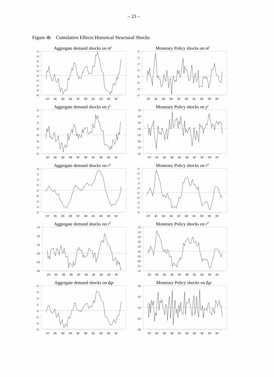
Figure 4b Cumulative Effects Historical Structural Shocks

1979 1981 1983 1985 1987 1989 1991 1993 1995 1997-0.8

-0.6

-0.4

-0.2

-0.0

0.2

0.4

0.6

0.8

1.0

1979 1981 1983 1985 1987 1989 1991 1993 1995 1997-2.4

-1.6

-0.8

-0.0

0.8

1.6

2.4

3.2

1979 1981 1983 1985 1987 1989 1991 1993 1995 1997-2.0

-1.5

-1.0

-0.5

0.0

0.5

1.0

1.5

2.0

1979 1981 1983 1985 1987 1989 1991 1993 1995 1997-0.50

-0.25

0.00

0.25

0.50

0.75

1979 1981 1983 1985 1987 1989 1991 1993 1995 1997-0.3

-0.2

-0.1

-0.0

0.1

0.2

0.3

0.4

1979 1981 1983 1985 1987 1989 1991 1993 1995 1997-1.5

-1.0

-0.5

0.0

0.5

1.0

1.5

2.0

1979 1981 1983 1985 1987 1989 1991 1993 1995 1997-1.60

-1.20

-0.80

-0.40

-0.00

0.40

0.80

1.20

1979 1981 1983 1985 1987 1989 1991 1993 1995 1997-2.0

-1.5

-1.0

-0.5

0.0

0.5

1.0

1.5

2.0

2.5

1979 1981 1983 1985 1987 1989 1991 1993 1995 1997-1.00

-0.75

-0.50

-0.25

0.00

0.25

0.50

0.75

1.00

1.25

1979 1981 1983 1985 1987 1989 1991 1993 1995 1997-0.50

-0.25

0.00

0.25

0.50

Aggregate demand shocks on mr

Aggregate demand shocks on yr

Aggregate demand shocks on rs

Aggregate demand shocks on rl

Aggregate demand shocks on ∆p

Monetary Policy shocks on mr

Monetary Policy shocks on yr

Monetary Policy shocks on rs

Monetary Policy shocks on rl

Monetary Policy shocks on ∆p

– 24 –

Figure 4c Cumulative Effects Historical Structural Shocks

1979 1981 1983 1985 1987 1989 1991 1993 1995 1997-0.3

-0.2

-0.1

-0.0

0.1

0.2

0.3

1979 1981 1983 1985 1987 1989 1991 1993 1995 1997-0.75

-0.50

-0.25

0.00

0.25

0.50

0.75

1979 1981 1983 1985 1987 1989 1991 1993 1995 1997-0.20

-0.15

-0.10

-0.05

-0.00

0.05

0.10

0.15

0.20

1979 1981 1983 1985 1987 1989 1991 1993 1995 1997-0.20

-0.15

-0.10

-0.05

-0.00

0.05

0.10

0.15

0.20

1979 1981 1983 1985 1987 1989 1991 1993 1995 1997-1.00

-0.75

-0.50

-0.25

0.00

0.25

0.50

0.75

1.00

1.25

Exchange rate shocks on mr

Exchange rate shocks on yr

Exchange rate shocks on rs

Exchange rate shocks on rl

Exchange rate shocks on ∆p

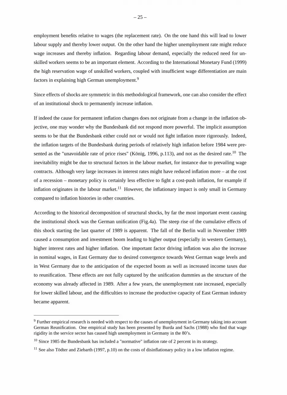
– 25 –

employment benefits relative to wages (the replacement rate). On the one hand this will lead to lower

labour supply and thereby lower output. On the other hand the higher unemployment rate might reduce

wage increases and thereby inflation. Regarding labour demand, especially the reduced need for un-

skilled workers seems to be an important element. According to the International Monetary Fund (1999)

the high reservation wage of unskilled workers, coupled with insufficient wage differentiation are main

factors in explaining high German unemployment.9

Since effects of shocks are symmetric in this methodological framework, one can also consider the effect

of an institutional shock to permanently increase inflation.

If indeed the cause for permanent inflation changes does not originate from a change in the inflation ob-

jective, one may wonder why the Bundesbank did not respond more powerful. The implicit assumption

seems to be that the Bundesbank either could not or would not fight inflation more rigorously. Indeed,

the inflation targets of the Bundesbank during periods of relatively high inflation before 1984 were pre-

sented as the "unavoidable rate of price rises" (König, 1996, p.113), and not as the desired rate.10 The

inevitability might be due to structural factors in the labour market, for instance due to prevailing wage

contracts. Although very large increases in interest rates might have reduced inflation more – at the cost

of a recession – monetary policy is certainly less effective to fight a cost-push inflation, for example if

inflation originates in the labour market.11 However, the inflationary impact is only small in Germany

compared to inflation histories in other countries.

According to the historical decomposition of structural shocks, by far the most important event causing

the institutional shock was the German unification (Fig.4a). The steep rise of the cumulative effects of

this shock starting the last quarter of 1989 is apparent. The fall of the Berlin wall in November 1989

caused a consumption and investment boom leading to higher output (especially in western Germany),

higher interest rates and higher inflation. One important factor driving inflation was also the increase

in nominal wages, in East Germany due to desired convergence towards West German wage levels and

in West Germany due to the anticipation of the expected boom as well as increased income taxes due

to reunification. These effects are not fully captured by the unification dummies as the structure of the

economy was already affected in 1989. After a few years, the unemployment rate increased, especially

for lower skilled labour, and the difficulties to increase the productive capacity of East German industry

became apparent.

9 Further empirical research is needed with respect to the causes of unemployment in Germany taking into accountGerman Reunification. One empirical study has been presented by Burda and Sachs (1988) who find that wagerigidity in the service sector has caused high unemployment in Germany in the 80’s.

10 Since 1985 the Bundesbank has included a "normative" inflation rate of 2 percent in its strategy.

11 See also Tödter and Ziebarth (1997, p.10) on the costs of disinflationary policy in a low inflation regime.

– 26 –

A positive institutional shock positively affects output, interest rates and inflation, and decreases real

money holdings (Fig.2a). Especially long-term interest rates are dominated by this shock. The decrease

in real money holdings despite the increase in output is explained by the higher opportunity costs of

holding money. According to the forecast error variance decompositions, institutional shocks dominate in

the long run, especially with respect to long-term interest rates, output and real money balances (Fig.3a).

The positive aggregate demand shock (Fig.2b) has a significant positive effect on output and a positive,

although not significant, effect on inflation. Higher inflation is reflected in an increase in nominal interest

rates. By assumption, all effects are transitory for this shock. In the short run about 25% of the variance of

output can be explained by the demand shock. As this shock is transitory, in the long run the contribution

is negligible.

A shock in the interest rate can be interpreted as the transitory and unexpected element of monetary

policy. A positive interest rate shock leads to an increase in nominal short- and long-term interest rates

and therefore invokes an immediate drop in the inflation rate and a small but insignificant decrease in

output (Fig.2b). The immediate price reaction might be explained by an instantaneous appreciation of

the DM.12 The negative inflation effect only lasts for one quarter however, which casts some doubts on

the interpretation of this shock as a monetary policy shock. Real money balances increase initially even

though output decreases and long-term interest rates increase. Apparently, the short term interest rate,

which represents the own interest rate of the interest bearing items in M3, is more important for money

demand in the short run. As the increase in real money balances is much bigger contemporaneously than

the decrease in prices, controllability is problematic in the short run. In the long run both real money

balances and the price level are hardly affected. For real balances that has been imposed, but the price

level was not restricted. Therefore, we find no convincing evidence that money was controllable by the

Bundesbank. In this type of analysis the model endogenizes the monetary policy rule, i.e. anticipated

policy actions of the monetary authorities are implicit in the system analysed. However, some of the

structural shocks result in deviation of money from its target and we find that this deviation can not be

corrected by unanticipated monetary policy actions.

The fifth shock identified is interpreted as an exchange rate shock (Fig.2c). This might for instance

be due to foreign interest rate changes. The influence of domestic interest rates on the exchange rate is

modelled already in the previous shock. Inflation shows a sharp increase in the first period. This might

be due to a price rise of primary commodities for which the law of one price might be a reasonable

approximation. Already after one quarter inflation turns negative again. Output is positively affected by

the depreciation after one quarter. However, according to the variance decompositions, the size of this

12 Although monetary policy is usually assumed to affect inflation only with some lag, CV find a similar contem-poraneous monetary policy effect on inflation for the euro area that is reverted almost immediately.

– 27 –

effect is negligible. Only prices are significantly affected by this shock. In the short run, it even explains

almost 90% of inflation variability. According to the historical decompositions (Fig.4c), the exchange

rate shock is quite volatile. Maybe this shock also embodies other transitory volatile price movements

due to for instance changes in seasonal patterns or harvest conditions.

Regarding the causal link between money and inflation, our results do not provide evidence of a leading

role for money. In a monetary targeting strategy, the growth of the money stock as such is considered

to be indicative of future inflation, irrespective of the underlying reason for this growth. Consequently,

in principle all shocks should be considered in order to judge the leading indicator role of money. The

two shocks that affect money most are the technology and the institutional shock. For both shocks

there is a clear negative relation between money growth and subsequent inflation.13 For the aggregate

demand shock, there is a positive relation between real money and inflation, but money growth does not

lead inflation for this shock either. For the other two shocks either the impact on money or the one on

inflation is negligible. Consequently, we find no evidence of a leading role for money with respect to

inflation.

6.3 Robustness of the results

In evaluating the results of structural VAR analysis the literature has focussed on the sensitivity of the

findings (see e.g. Christiano, Eichenbaum and Evans, 1998). Therefore, this section discusses the robust-

ness of the impulse responses presented for Germany.

First, it has been analysed whether the results are sensitive regarding the inclusion of a different short-

term interest rate. The day-to-day interest rate that should be more closely related to the policy rate of

the Bundesbank (the repo rate) has been included instead of the 3-months money market rate. It turns

out that the impulse responses are robust towards the inclusion of the day-to-day interest rate.

An analysis of the sensitivity of the results towards changing the identification scheme shows that the

finding that it is impossible to split the common trends in either having only nominal or real effects

is robust with respect to different contemporaneous identification restrictions given the economically

motivated restriction that inflation is not affected by the technological shock in the long-run. The results

for the transitory shocks depend on the contemporaneous restrictions imposed. Especially the exchange

rate shock could be given a different interpretation if other restrictions were imposed. However, the

interpretation as an exchange rate shock appeared to be most plausible from an economic point of view.

Furthermore, the over-identifying restriction imposed on the system is not rejected.

13 This result is robust with respect to different identification schemes (see also Section 6.3).

– 28 –

Finally, sensitivity towards the lag order of the model has been investigated. The impulse responses of a

VAR(4) where a cointegration rank of three and three cointegration relations have been imposed display

much more volatility than for the VAR(2). The general results do not change, however.

– 29 –

7 TENTATIVE LESSONS FOR EMU

In order to learn to know more about the monetary transmission process in EMU, one would of course

like to use EMU data. However, as these data are only now becoming available an empirical analysis

can not be performed solely on these data for years. In the meantime aggregated euro area data over a

pre-EMU period can be used to get an impression of the likely EMU outcome. However, since many

countries have experienced relatively high inflation during part of this sample and moreover did not

follow an independent monetary policy, these results are likely to be biased. The German experience

can provide a second benchmark as the policy of the ECB is very similar to the one of the Bundesbank

and the low inflation environment is likely to be representative for EMU. Of course, these results are not

likely to be fully representative of EMU as other countries might respond differently to certain shocks

than Germany. However, as the biases in the two benchmarks are probably independent, results found

for both aggregated euro area data and German data can be considered relatively robust. If the two

approaches lead to different conclusions, further research seems warranted.

Comparing the findings of the present analysis with aggregate euro area studies, the process of identifi-

cation shows that to a large extent a similar pattern of shocks influences the German economy as in the

euro area as a whole. Regarding the common trends, the responses to the technological shock are similar

to supply shock responses in the aggregated euro area, except for the development of prices which adjust

later in Germany than in the euro area.

Probably the most important difference between the German and the aggregated European system is

that only for the latter the common trends can be split to have either nominal or real effects in the

long run. For Germany, a permanent decrease in inflation is accompanied by a permanent lower output

level. This result of our analysis for Germany is robust with respect to different identification schemes.

As explained, the absence of an output neutral monetary policy objective shock for Germany could be

due to the fact that the monetary policy objective hardly changed over our sample. Consequently, this

shock is not important for Germany. Nevertheless, given the ultimate dominance of the institutional

shock in Germany as shown by the variance decompositions, it is surprising that for the euro area no

shock occurs that implies both nominal and real effects in the long run. The importance of the long run

positive correlation between inflation and output in Germany might partly be explained by the German

reunification. In addition, the fact that Germany was the anchor country for inflation during the EMS

period is probably important. Being the leading country higher (or lower) inflation in Germany was

sustainable without affecting output due to the fact that many other countries implicitly adjusted their

inflation target to the German outcome. Consequently, real exchange rates were hardly affected. For most

other EMS countries the external target of a fixed D-mark rate probably helped in reducing wage pressure

– 30 –

during a tense labour market. Finally, institutional shocks might be less prominent in the aggregated data

because they partly cancel between countries if they operate in an asynchronous fashion.

The euro area will probably feature elements of both the German and of the aggregated European data.

As the inflation target for the ECB is not likely to change, the inflation objective shock as identified for

the aggregated European data is probably not relevant for EMU. The relevance of shocks that affect both

output and inflation permanently probably depends on the extent to which these structural shocks will

be synchronous. As far as the shocks that permanently affect output are asynchronous, the inflationary

impact will probably be limited. Synchronous shocks on the other hand might affect inflation somewhat,

provided that there is some flexibility in the price stability target of the ECB.

The response pattern of the variables to a positive aggregate demand shock looks similar in Germany

and the euro area (see Coenen and Vega, 1999). However, the contemporaneous increase in output due

to a positive aggregate demand shock is about twice as large for Germany than for the euro area. Real

money holdings are hardly affected in Germany whereas for the euro area CV find a positive and VS find

a negative response of money holdings which they explain by lower precautionary saving in an economic

upswing.

The variables also display a similar response pattern due to an interest rate shock in Germany and for

the euro area (see Coenen and Vega, 1999). CV found a similar implausibly large contemporaneous

inflation effect that was reverted after one quarter. However, in their system the long run overall price

effect is slightly negative, although insignificantly so, whereas we find a negligible positive price effect.

Consequently, according to these results controllability of the nominal money stock might even have

been more problematic for the Bundesbank than it will be for ECB.

Also with respect to the causal link between money growth and inflation the results for Germany alone

are just as disappointing as for the European aggregates. Based on SVAR analysis, there appears to be

no evidence for the leading indicator role of money for either Germany or the euro area.

– 31 –

8 CONCLUSIONS

This paper has analysed the transmission of monetary policy in Germany for a sample covering the EMS

period from 1979(1) to 1998(4) and compared the results to studies analysing constructed aggregated

euro area data for the pre-EMU period using the same methodological framework. The findings indicate

that investigating the German experience can provide useful insigths for the common monetary policy in

EMU as another benchmark besides the analysis of aggregated euro area data.

The results for Germany appear to a large extent similar to the response patterns found for aggregated

euro area data, even though the identification restrictions differ to some extent. However, important

differences also arise. The main difference between the European and the German system is that for

Germany one common trend involves both nominal and real effects in the long run, whereas for Europe

a distinction could be made between nominal and real shocks. This combined shock results in a positive

correlation in the long run between the output level and inflation. We contribute this shock to institutional

changes, primarily related to the structural unemployment. Consequently, we assume that the permanent

changes in the inflation rate in Germany originated in the real economy and were not due to a change in

monetary policy objectives, given the low inflation culture of the Bundesbank. An underlying assumption

is that monetary policy is less effective during labour market pressure.

It can be argued that, at least in spirit, the environment under which the ECB has to operate is more

similar to that of the Bundesbank (low inflation, no exchange rate target) than that of the European

average. On the other hand competition in terms of unit labour cost between euro-members that was

probably an important factor in a successful disinflationary policy before is likely to become even more

important now the individual currencies are irrevocably linked. Consequently, further research is needed

in order to shed light on the cost of disinflation in Europe.

Regarding a monetary targeting strategy, the results are very similar to previously found results for euro

area aggregates. We do find evidence of a stable money demand relationship, but our analysis also indi-

cates problems with respect to the controllability and the leading indicator role of money. Controllability

of nominal money seems seriously impaired in the short run, whereas in the long run money is hardly

affected by interest rate shocks. The implausible inflation pattern resulting from these shocks prevents

strong conclusions about controllability however. The leading role for money in predicting inflation for

Germany could not be confirmed by our analysis. These results suggest that the role of money targets in

the successful strategy of the Bundesbank of controlling inflation should not be overemphasised.

– 32 –

APPENDIX A STABILITY TESTS

1990 1995 2000

.5

1 5% 1up m_r

1990 1995 2000

.5

1

5% 1up y_r

1990 1995 2000

.5

1 5% 1up R_s0

1990 1995 2000

.5

1 5% 1up R_l0

1990 1995 2000

.5

1 5% 1up Dp

1990 1995 2000

.5

1 5% 1up CHOWs

(a) 1 step Chow test (1.0: 5% significance level)

1990 1995 2000

.5

.75

1 5% Ndn m_r

1990 1995 2000

.25

.5

.75

1 5% Ndn y_r

1990 1995 2000

.5

1 5% Ndn R_s0

1990 1995 2000

.25

.5

.75

1 5% Ndn R_l0

1990 1995 2000

.25

.5

.75

1 5% Ndn Dp

1990 1995 2000

.5

.75

1 5% Ndn CHOWs

(b) Break-point Chow Test (1.0: 5% significance level)

– 33 –

APPENDIX B COINTEGRATION ANALYSIS

Unit root tests have been carried out for the data (see Table 3). For money and output the Perron (1989)

(model A, level shift) test has been used to take account of the level shift in these variables due to the

German unification. For the other variables the augmented Dickey Fuller test is used. All variables

appear to be I(1).

Table 3 Perron Test / Augmented Dickey Fuller Test

variable auxiliary regression k t-statistic critical value(in log) (5%)

mr c, t,D902,SD 1 −2.17 −3.76(1)

yr c, t,D911,SD 5 −1.93 −3.76(1)

rs c 5 −2.78 −2.90

rl c 4 −1.81 −2.90

∆p c,SD 4 −2.31 −2.90

∆mr c,D902i,SD 5 −4.60∗∗ −2.90

∆yr c,D911i,SD 4 −3.93∗∗ −2.90

∆rs c 1 −4.91∗∗ −2.90

∆rl c 3 −3.71∗∗ −2.90

∆∆p c,SD 4 −9.31∗∗ −2.90Notes: k : is the number of lagged differences included in the DF/ADF test (ac-

cording to the highest significant number of lags with a maximum of 5 lags);

** and *: significance at a 1% and 5% level; critical values from MacK-

innon (1991), sample period 1979(1)-1998(4), except for (1): critical value

of Model(A) in Perron (1989), λ = 0.60, c: constant, t: linear trend, D902,

D911: step dummies (1 after 1990(2) and 1991(1) respectively, 0 otherwise,

D902i,D911i: impulse dummies (1 in 1990(2) and 1991(1) respectively), SD:

seasonal dummies

Johansen’s likelihood ratio (LR) trace test has been applied to test for the cointegration rank of the five

variable system.14

The test indicates a cointegration rank of r = 4 on a 5% significance level.15 In our five variable system

without trend, a rank of four would imply stationary interest rates, inflation rate and a relation between

14 For a review of different cointegration rank tests, see for example Hubrich, Lütkepohl and Saikkonen (2001)and also Hubrich (1999) focussing on the small sample performance of different systems cointegration tests.

15 The largest cointegration rank tested is r0 = n− 2 = 3 because a linear trend in the data is allowed by thespecification of the model. This excludes the possibility of n = r, i.e. n stationary variables. Therefore, r0 = n−1is not a reasonable null hypothesis (see also Saikkonen and Lütkepohl, 2000).

– 34 –

Table 4 Johansen’s LR Test, 5-dimensional VAR(2), Det. Terms: Constant, SD, D902, D911, D9334

and D944, Estimation Period: 1979(1)-1998(4)

H0: rank=r0 LR 95%

trace critical values

statistic

r0 = 0 122.2 68.5

r0 = 1 47.9 47.2

r0 = 2 30.5 29.7

r0 = 3 16.1 15.4Note: critical values are the 95% quantiles of the

asymptotic distribution: Johansen (1995).

money and output.16 Since interest rates and inflation are clearly indicated to be I(1) variables according

to the Dickey Fuller test statistics, a rank of four seems unlikely. Figure 8 shows the stability of the

cointegration rank for our system. Only for the system including the last quarter, a rank of four is

supported. For a sample until 1997 however - might be reasonable to consider because relations are

probably distorted for 1998 shortly before the start of EMU - the cointegration rank is r = 3. For shorter

samples a rank between one and three is indicated. Given the intuitive economic interpretation, and in

line with Hubrich (1999, 2001) for a similar set variables in a shorter sample period, a rank of three was

imposed.

STABILITY OF THE COINTEGRATION RANK: THE Z-MODELSIGNIFICANCE LEVEL= 95%

1989 1990 1991 1992 1993 1994 1995 1996 1997 19980.0

0.2

0.4

0.6

0.8

1.0

1.2

1.4

1.6

1.8

Figure 5 Recursive cointegration rank

16 If a restricted trend is included, the cointegrating rank would be only one. However, both under a rank of oneand under a rank of four, the null hypothesis that the restricted trend can be excluded is not rejected employing anLR-test (see Johansen (1995, p.162)).

– 35 –

APPENDIX C S-VECM METHODOLOGY

This section provides a brief summary of Vlaar (1998). Let xt be a n−dimensional vector of variables

which is generated by an unrestricted vector autoregressive (VAR) process of order k

xt = µ+A1xt−1 + . . .+Akxt−k + εt (1)

where µ is a vector of constants, Ais are (n×n)−dimensional coefficient matrices and where the vector

of innovations εt has covariance matrix E(εtε′t) = Σ. If xt is cointegrated of order (1,1) with cointegrating

rank r, then, according to the Engle/Granger representation (see Engle and Granger (1987) or Johansen

(1995)), the data generating process has two equivalent representations:

a) the vector error correction representation

∆xt = µ+αβ′xt−1 +Γ1∆xt−1 + . . .+Γk−1∆xt−k+1 + εt (2)

where α,β are (n× r)−dimensional full column rank matrices and Γis represent (n× n)−dimensional

coefficient matrices, and

b) the vector moving average representation

∆xt = C(L)(µ+ εt) (3)

where C(L) ≡ In −∑∞i=1CiLi is a matrix polynomial of infinite order in the lag operator L, and C(1) =

β⊥(

α′⊥(In −∑k−1

i=1 Γi)β⊥)−1

α′⊥. The C(1) matrix, which has rank n− r, gives the ultimate effect of a

shock to the reduced form innovations on the level of the endogenous variables.

The structural vector error correction model (S-VECM) method is a two stage procedure. In the first stage

the reduced form vector error correction model (Equation 2) is estimated. The second step comprises in

the identification of the structural model. Thereto it is assumed that the reduced form disturbances εt are

linearly related to an n−dimensional vector of orthonormal structural innovations et :

εt = B0et with E(ete′t) = In (4)

where B0 is a non-singular (n×n) matrix. In order to identify the structural model, restrictions have to be

imposed on the B0 matrix. From the relationship between the variances of the reduced form residuals and

the structural innovations it follows that B0B′0 = Σ. This relationship imposes n(n + 1)/2 independent

restrictions on B0, leaving n(n−1)/2 elements free. Consequently n(n−1)/2 additional independent re-

strictions have to be imposed in order to exactly identify the structural model.17 Once at least n(n−1)/2

17 One might also impose more restrictions, in which case the model will be over-identified.

– 36 –

independent restrictions have been imposed, the B0 matrix can be estimated by maximum likelihood.

Assuming the restrictions are all linear zero restrictions, this boils down to maximizing:

logl = −T2

log(|B0|2

)− T2

tr(B′−1

0 B−10 Σ̂

)subject to Rvec(B0) = 0 (5)

where Σ̂ denotes the estimated covariance matrix of the residuals of the first step, R denotes a (g× n2)

matrix, imposing the g independent restrictions on B0 and vec() denotes the column stacking operator.

In the case of only contemporaneous restrictions, the R matrix is a selection matrix with only nonzero

elements for the restricted elements of B0. Long run restrictions are related to the C(1) matrix. If the jth

structural innovation is supposed to have no impact on variable i in the long run, this can be achieved by

restricting the i, j element of B∞ ≡C(1)B0 to be zero.18

Given the rank of n− r for C(1), at most (n− r)(r + (n− r − 1)/2) independent long run restrictions

can be imposed. Consequently, at least r(r − 1)/2 contemporaneous restrictions are needed. In the

common trends representation (see Stock and Watson (1988)), only n− r structural shocks (the common

trends) are supposed to drive the system in the long run, whereas the impact of the other r structural

shocks (the transitory shocks) dies out in the long run. In our model this structure can be imposed by

restricting r columns of B∞ to zero. As the rank of C(1) is n− r, this implies r(n− r) independent

restrictions. The mutual identification of the common trends can subsequently be achieved by imposing

either contemporaneous or long-run restrictions. For the identification of the transitory shocks, only

contemporaneous restrictions can be used.

The asymptotic distribution of the impulse response functions in case of only contemporaneous restric-

tions is given in Lütkepohl and Reimers (1992). The introduction of long run restrictions considerably

complicates the distribution however, as these restrictions on B0 are functions of the VECM parameters.

As a consequence, the convenient block-diagonality of the covariance matrix of model parameters with

the parameters of the mean on the one hand and those of B0 on the other hand is destroyed. In Vlaar

(1998) it is shown that the asymptotic distribution of the impulse responses can still be computed from

the covariance matrix that neglects the stochastic nature of these restrictions however, provided that a

correction is computed related to the partial derivative of B0 with respect to the VECM parameters.

18 The long-run restrictions are on structural parameters (B0) in contrast to Paruolo (1997) who proposes to imposerestrictions on the long-run impact matrix (C(1)).

– 37 –

APPENDIX D DATA

The data analysed in this paper are quarterly, not seasonally adjusted time series for the period 1979(1)

to 1998(4). Sources are as follows:

– The nominal M3 time series are obtained from the data bank DATASTREAM and are originally

obtained from the Deutsche Bundesbank. The time series is given in billion DM. The value of the last

month of each quarter represents the quarterly value. The structural break of German reunification is in

1990(2).

– The GDP data are in constant prices with 1991 as the basis year. East-Germany is included from

1991(1) onwards. The data are from DATASTREAM, originating from the Quarterly National Accounts

of the OECD.

– Prices are represented by the deflator of GDP (1991=100) derived from Bundesbank data offered in

DATASTREAM, i.e. GDP in current prices (in billion DM) divided by GDP in constant prices.

– The long-term interest rate is the long-term interest rate on 10 year government bonds from DATA-

STREAM originally provided by the BIS. These data are quarterly averages.

– The three-months short-term interest rate is the euro market rate from DATASTREAM, originally

provided by the BIS. These data are quarterly averages.

– The day-to-day interest rate is taken from DATASTREAM, originally provided by the Deutsche

Bundesbank. These data are quarterly averages.

– 38 –

REFERENCES

Benkwitz, A., Lütkepohl, H. and Wolters, J., 2000, ‘Comparison of bootstrap confidence intervals for

impulse responses of German monetary systems’, Macroeconomic Dynamics, forthcoming.

Bernanke, B. S. and Mihov, I., 1997, ‘What does the Bundesbank target?’, European Economic Review

41, 1025–1053.

Beyer, A., 1998, ‘Modelling money demand in Germany’, Journal of Applied Econometrics 13, 57–76.

Blanchard, O. J. and Quah, D., 1989, ‘The dynamic effects of aggregate demand and supply distur-

bances’, American Economic Review 79, 655–673.

Blanchard, O. J., 1989, ‘A traditional interpretation of economic fluctuations’, American Eocnomic

Review 79, 1146–1164.

Brüggemann, I., 1999, ‘Inflation versus monetary targeting in Germany’, Discussion paper, Freie

Universität.

Burda, M. C. and Sachs, J. D., 1988, ‘Assessing high unemployment in West Germany’, The World

Economy 11(4), 543–563.

Burda, M. C., 1991, ‘Structural change, unemployment benefits and high unemployment: A US-

European comparison’, The Art of Full Employment, Elsevier Science Publishers B.V., North-

Holland, pp. 399–422.

Cabos, K., Funke, M. and Siegfried, N. A., 1999, ‘Some thoughts on monetary targeting vs. inflation

targeting’, Quantitative Macroeconomics Working Paper 8/99, Universität Hamburg.

Christiano, L. J., Eichenbaum, M. and Evans, C. L., 1998, ‘Monetary policy shocks: What have we

learned and to what end?’, Working Paper 6400, National Bureau of Economic Research.

Clarida, R. and Gertler, M., 1996, ‘How the Bundesbank conducts monetary policy’, Working Paper

5581, National Bureau of Economic Research.

Coenen, G. and Vega, J.-L., 1999, ‘The demand for M3 in the euro area’, Working Paper Series 6,

European Central Bank, http://www.ecb.int.

Engle, R. F. and Granger, C. W. J., 1987, ‘Cointegration and error correction: Representation, estima-

tion and testing’, Econometrica 55, 251–276.

Ericsson, N. R., Hendry, D. F. and Mizon, G. E., 1998, ‘Exogeneity, cointegration, and economic

policy analysis’, Journal of Business and Economic Statistics 16(4), 370–387.

– 39 –

Fagan, G. and Henry, J., 1998, ‘Long run money demand in the EU: Evidence for area-wide aggre-

gates’, Empirical Economics 23(3), 483–506.

Fase, M. M. G. and Winder, C. C. A., 1993, ‘The demand for money in the Netherlands and the other

EC countries’, De Economist 141(4), 471–496.

Fase, M. M. G. and Winder, C. C. A., 1998, ‘Wealth and the demand for money in the European

Union’, Empirical Economics 23(3), 507–524.

Fung, B. S.-C. and Kasumovich, M., 1998, ‘Monetary shocks in the G-6 countries: Is there a puzzle?’,

Journal of Monetary Economics 42, 575–592.

Gali, J., 1992, ‘How well does the IS-LM model fit postwar U.S. data?’, Quarterly Journal of Economics

107(2), 819–840.

Gerlach, S. and Smets, F., 1995, ‘The monetary transmission mechanism: Evidence form the G-7

countries’, Discussion Paper 1219, CEPR.

Gonzalo, J. and Ng, S., 1996, ‘A systematic framework for analysing the dynamic effects of permanent

and transitory shocks’, mimeo. Universidad Carlos III de Madrid.

Hubrich, K., Lütkepohl, H. and Saikkonen, P., 2001, ‘A review of systems cointegration tests’,

Econometric Reviews, forthcoming.

Hubrich, K., 1999, ‘Estimation of a German money demand system - A long-run analysis’, Empirical

Economics 24(1), 77–99.

Hubrich, K., 2001, Cointegration Analysis in a German Monetary System, Physica-Verlag, Heidel-

berg/New York.

International Monetary Fund, 1999, ‘Germany: Selected issues and statistical appendix’, IMF Staff

Country Report 99/130.

Issing, O. and Tödter, K.-H., 1995, ‘Geldmenge und Preise im vereinten Deutschland’, in D. Duwendag

(ed.), Neuere Entwicklungen in der Geldtheorie und Währungspolitik, Duncker & Humblot, Berlin,

pp. 97–123.

Issing, O., 1997, ‘Monetary targeting in Germany: The stability of monetary policy and of the monetary

system’, Journal of Monetary Economics 39, 67–79.

Johansen, S., 1995, Likelihood-based inference in cointegrated vector autoregressive models, Oxford

University Press, Oxford.

– 40 –

Juselius, K., 1996, ‘The changing role of the German Bundesbank. An empirical analysis of German

monetary policy before and after 1983’, Oxford Bulletin of Economics and Statistics 58, 791–819.

King, R. G., Plosser, C. I., Stock, J. H. and Watson, M. W. , 1991, ‘Stochastic trends and economic

fluctuations’, The American Economic Review 81, 819–840.

König, R., 1996, ‘The Bundesbank’s experience of monetary targeting’, in Deutsche Bundesbank (ed.),

Monetary Strategies in Europe, Verlag Vahlen, München, pp. 107–140.

Lütkepohl, H. and Reimers, H.-E., 1992, ‘Impulse response analysis of cointegrated systems’, Journal

of Economic Dynamic and Control 16, 53–78.

Lütkepohl, H. and Wolters, J., 1998, ‘A money demand system for German M3’, Empirical Economics

23(3), 371–386.

MacKinnon, J. G., 1991, ‘Critical values for co-integration tests’, in R. Engle and C. Granger (eds),

Long-Run Economic Relationships, Oxford University Press, pp. 267–76.

Mellander, E., Vredin, A. and Warne, A., 1992, ‘Stochastic trends and economic fluctuations in a

small open economy’, Journal of Applied Econometrics 7, 368–394.

Mittnik, S. and Zadrozny, P., 1993, ‘Asymptotic distributions of impulse responses, step responses,

and variance decompositions of estimated linear dynamic models’, Econometrica 61, 857–870.

Monticelli, C. and Papi, L., 1996, European Integration, Monetary Coordination and the Demand for

Money, Oxford University Press, Oxford.

Monticelli, C. and Tristani, O., 1999, ‘What does the single monetary policy do? A SVAR

benchmark for the European Central Bank’, Working Paper Series 2, European Central Bank,

http://www.ecb.int.

Paruolo, P., 1997, ‘Asymptotic inference on the moving average impact matrix in cointegrated I(1)

systems’, Econometric Theory 13, 79–118.

Perron, P., 1989, ‘The great crash, the oil price shock, and the unit root hypothesis’, Econometrica

57(6), 1361–1401.

Pesaran, M. H., Pierse, R. G. and Kumar, M. S., 1989, ‘Econometric analysis of aggregation in the

context of linear prediction models’, Econometrica 57, 861–888.

Rudebusch, G. D., 1998, ‘Do measures of monetary policy in a VAR make sense?’, International

Economic Review 39(4), 907–931.

– 41 –

Saikkonen, P. and Lütkepohl, H., 2000, ‘Testing for the cointegrating rank of a VAR process with

structural shifts’, Journal of Business and Economics Statistics, forthcoming.

Schächter, A. and Stokman, A. C. J., 1995, ‘Interest rate policy of the Deutsche Bundesbank: An

econometric analysis for 1975 to 1992’, De Economist 143, 475–494.

Sims, C. A., 1980, ‘Macroeconomics and reality’, Econometrica 48, 1–48.

Stock, J. H. and Watson, M. W., 1988, ‘Testing for common trends’, Journal of the American Statistical

Association 83, 1097–1107.

Tödter, K.-H. and Ziebarth, G., 1997, ‘Price stability vs. low inflation in Germany: An analysis of

costs and benefits’, Working Paper 6170, National Bureau of Economic Research.

Vlaar, P. J. G. and Schuberth, H., 1999, ‘Monetary transmission and controllability of money in

Europe: A structural vector error correction approach’, Staff Reports 36, De Nederlandsche Bank,

http://www.dnb.nl.

Vlaar, P. J. G., 1998, ‘On the asymptotic distribution of impulse response functions with long run

restrictions’, Staff Reports 22, De Nederlandsche Bank, http://www.dnb.nl.

Wesche, K., 1997, ‘The stability of European money demand: An investigation of M3H’, Open

Economies Review 8(4), 371–391.

Wolters, J., Teräsvirta, T. and Lütkepohl, H., 1998, ‘Modelling the demand for M3 in the unified

Germany’, The Review of Economics and Statitistics 80(3), 399–409.