Money markets and bank lending: evidence from the adoption

Working Paper Series

Money markets and bank lending:

evidence from the adoption of tiering

Carlo Altavilla, Miguel Boucinha,

Lorenzo Burlon, Mariassunta Giannetti,

Julian Schumacher

Disclaimer: This paper should not be reported as representing the views of the European Central Bank

(ECB). The views expressed are those of the authors and do not necessarily reflect those of the ECB.

No 2649 / February 2022

Abstract Exploiting the introduction of the ECB’s tiering system for remunerating excess reserve holdings, we document the importance of access to the money market for bank lending. We show that the two-tier system produced positive wealth effects for banks with excess reserves and encouraged a reallocation of liquidity toward banks with unused exemptions. This ultimately decreased the fragmentation in the money market and enhanced the monetary policy transmission mechanism. The increased access to money markets by banks with unused allowances incentivizes them to extend more credit than other banks, including banks with excess liquidity whose valuations increase the most. JEL Codes: G2; E5

Keywords: Money market; bank lending; negative interest rate policy

ECB Working Paper Series No 2649 / February 2022 1

Non-technical summary

A number of theories emphasize the importance of the smooth functioning of money markets and

the reallocation of liquidity for bank lending. However, shocks affecting the functioning of the

money market may also affect the demand for credit, making it hard to identify the actual

importance of money markets in empirical studies, especially during non-crisis periods.

This paper exploits a quasi-natural experiment created by a policy of the European Central Bank

(ECB) to shed light on the importance of the smooth functioning of the money market for bank

lending. The euro area is an ideal setting to explore the consequences of frictions in the money

market because, following the global financial crisis, money market segmentations and rate

dispersion had raised concerns regarding the transmission of monetary policy.

The revival of the unsecured market was driven by a policy enacted by the ECB in 2019.

Specifically, the ECB, as other central banks operating negative interest rate policies (NIRPs)

before, introduced a tiering system for the remuneration of central bank reserves held by

commercial banks. The ultimate goal of the tiering system was to mitigate the potential side effects

associated with negative interest rates and to support the bank-based transmission of monetary

policy by exempting a share of excess liquidity holdings from the application of the negative

deposit facility rate (DFR).

We show that improved money market conditions driven by the implementation of the tiering

enhanced the transmission of monetary policy to credit conditions in the economy. More

specifically, by revitalizing the money market activity through the reallocation of unused

exemption allowances across intermediaries, the tiering system increased the availability of short-

term wholesale funds. This in turn decreased banks’ incentives to pile up precautionary liquidity

buffers and stimulated interbank lending. The associated reduction in segmentation ultimately

supported loan supply to the non-financial private sector, which strengthened the transmission of

monetary policy.


1. Introduction

A number of theories emphasize the importance of the smooth functioning of money

markets and the reallocation of liquidity for bank lending (Caballero and Krishnamurthy, 2008;

Allen, Carletti, and Gale, 2009; Diamond and Rajan, 2011; Bolton, Santos and Scheinkman, 2011).

However, shocks affecting the functioning of the money market may also affect the demand for

credit, making it hard to identify the actual importance of money markets in empirical studies,

especially outside crisis periods.

This paper exploits a quasi-natural experiment created by a policy of the European Central

Bank (ECB) to shed light on the importance of the smooth functioning of the money market for

bank lending. The euro area is an ideal setting to explore the consequences of frictions in the

money market because, following the global financial crisis, money market segmentations and rate

dispersion had raised concerns regarding the transmission of monetary policy (Corradin et al.,

2020). The unsecured money market had lost importance, due to high perceived counterparty risk,

increased regulatory costs of unsecured transactions, and the significant rise in excess liquidity

following the ECB’s unconventional monetary policy measures. Thus, while the times were

tranquil and the market was far from frozen, it was largely dormant. In this context, we explore to

what extent a decrease in the frictions hampering banks’ access to outside liquidity affects lending

policies.

Money market activity was revitalized by a policy enacted by the ECB in 2019.

Specifically, the ECB, as other central banks operating negative interest rate policy (NIRP),

introduced a tiering system for the remuneration of central bank reserves held by commercial

banks. The ultimate goal of the tiering system was to support the bank-based transmission of

monetary policy while mitigating the potential side effects associated with negative interest rates


by exempting a share of excess liquidity holdings from the application of the negative deposit

facility rate (DFR). Concretely, tiering systems exempt from negative rates a fraction – the

“exempt tier” – of the liquidity deposited with the central bank in excess of the minimum reserve

requirements, which are mandated by regulation. This intervention has a direct positive effect on

the profitability of banks, as they avoid being “taxed” on part of their liquidity holdings.

Importantly, to avoid an unintended tightening in bank funding conditions, tiering systems are

calibrated such that the “non-exempted tier” – the amount of excess liquidity that remains subject

to negative interest rates – is sufficiently large to avoid upward pressure on money market rates.

In this manner, central banks introducing a tiering system intend not to impair the transmission of

monetary policy to money market interest rates and, if anything, to enhance it, because reducing

the costs of banks’ reserve holdings mitigates the negative effects of NIRP on intermediation

margins.

We show that the valuations of banks with more excess liquidity, which expect larger

savings from the tiering system, increase to a larger extent in expectation of the tiering system

adoption. More interestingly, the ECB intervention appears to enhance the transmission

mechanism by reducing money market segmentations and spurring a reallocation of excess

liquidity to banks with unused tiering allowances and ex ante low liquidity holdings. Enhanced

access to the money market in turn supports bank lending to the real sector.

The specific sequence of policy communication on the introduction of the tiering system

in the euro area facilitates the identification of the policy’s effectiveness. While the possible

introduction of a tiering mechanism was already anticipated in March 2019, the decision to

introduce a tiering system was formally announced in September 2019 and became effective at the

end of October of the same year. Markets considered an informal discussion in a March 2019


speech by the ECB’s president to be a credible signal about the possible adoption of a tiering

system, as bank valuations substantially increased in the immediacy of the announcement, but the

actual exemptions and the reallocation of liquidity occurred only at the end of October.1

We show that following the first discussion on the tiering, banks with relatively high

liquidity holdings ex ante – whose savings would be higher ex post – experienced higher abnormal

returns. However, to maximize the value from the eventual implementation of the tiering system,

banks would need to hold just as much liquidity as would eventually be exempt from paying

negative rates. The expected value of liquidity thus increased for banks with “unused allowances”,

i.e., for those institutions holding less liquidity than they could exempt from negative rates.

Consistent with this conjecture, we observe that banks with unused allowances started to

gradually increase their excess liquidity holdings. After the official announcement and

implementation of the tiering system, the fragmentation in the money market decreased with the

number of bank counterparties in the money market increasing. Banks with unused exemptions

were able to obtain larger amounts of excess liquidity by increasing their net borrowing in the

money market. This holds even for banks borrowing from the same counterparty, suggesting that

the introduction of tiering allowed for the reintegration of these banks in the money marked. Banks

with unused allowances also reduced their bond holdings. Since bonds are used as collateral in

money market transactions, bond sales suggest a decrease in precautionary behavior leading banks

to hoard less collateral.

Reduced fragmentation in the money market appears to enhance the monetary policy

transmission mechanism. Banks with ex ante high unused allowances that had more difficult

1 The March 2019 informal announcement also contained a signalling component because the possible implementation of the two-tier system was interpreted by market participants as opening the possibility for protracting the negative interest rate policy for a more extended period.


access to the money market, as suggested by higher borrowing rates prior to the implementation

of the system in October 2019, extend more credit after the implementation of the tiering. They

also grant loans at lower rates and with longer maturity.

Our paper contributes to evaluate the importance of the money market and banks’ liquidity

hoarding in a non-crisis period. In this respect, it complements the findings of Afonso, Kovner and

Schoar (2011) and Acharya and Merrouche (2013), who show that counterparty risk hampered the

functioning of the US money market in the aftermath of Lehman’s default. We show that in normal

times, an increase in the benefits of reallocating liquidity reduces segmentations in the money

market and spurs lending to the real sector. Thus, banks’ ability to obtain liquidity through the

money market affects credit provision even when the money market is not frozen, not only during

financial crises, as shown by Iyer, Peydro, da-Rocha-Lopes, and Schoar (2014).

Besides evaluating the role of the money market, our paper contributes to understand the

transmission mechanism of monetary policy below the zero lower bound. Monetary policy

accommodation in low-interest-rate environments requires breaking the zero lower bound on

nominal interest rates (Rogoff, 2016; 2017). This might generate positive real economic effects by

incentivizing firms to invest more to avoid paying negative rates on their bank deposits (Altavilla,

Burlon, Giannetti, and Holton, 2021). However, NIRP might raise concerns about the stability of

the banking system if banks are not able to pass through negative rates to deposits because they

fear a flight to paper currency (Eggertsson, Juelsrud, Summers, and Wold, 2019) and because

regulation limits their ability to charge negative rates, especially on retail deposits. In the extreme

case, due to their negative effects on banks’ net interest income, negative rates may become

recessive as banks may cut lending if their net wealth decreases (Brunnermeier and Koby, 2016;


Ulate, 2021).2 By reducing the cost of holding excess liquidity, the tiering system directly supports

bank profits and can ultimately lead banks to expand their balance sheets and lend more.

Implications, however, are ambiguous. One mechanism through which negative policy

rates are believed to be transmitted to the real economy involves banks’ attempt to avoid paying

negative rates on their excess reserves. While aggregate excess reserve holdings in the banking

system as a whole are fixed, individual banks have been shown to increase lending in the attempt

to decrease their excess liquidity (Bottero, Minoiu, Peydró, Polo, Presbitero, and Sette, 2021).

In this context, the introduction of a tiering system affects banks’ incentives. On the one

hand, banks that have unfulfilled exemption allowances may have weaker incentives to lend,

undermining the transmission of monetary policy. On the other hand, after the introduction of the

tiering system, banks with unused exemptions may find it easier to borrow and to obtain excess

liquidity through the money market. The consequent reduction in banks’ precautionary behavior

may support lending. Which of these mechanisms prevails remains an empirical question. We

show that the introduction of a tiering system helps reduce segmentation in the money market and

spurs lending by banks with unused exemptions.

Notwithstanding many central banks have introduced tiering systems for reserve

remuneration, there are very few studies on their effectiveness. Fuster, Schelling and Towbin

(2021) shows that in Switzerland after the introduction of the tiering, banks that benefitted most

from the increase in the exemption threshold tend to charge higher loan spreads and take less risk

and that banks obtained liquidity by increasing the interest rate on deposits, effectively lowering

the pass-through. Their study captures the wealth effects of tiering systems. Our paper, instead,

2 The overall effects of the negative interest rates policy on bank profitability should also consider the positive general equilibrium effects from the increased monetary accommodation, both through higher intermediation volumes and improved borrower creditworthiness (see Altavilla, Boucinha, Peydró, 2018).


focuses on the implications of tiering for monetary policy transmission. We show that tiering

systems, by increasing the benefits of trading, improve the functioning of money markets and

stimulate bank lending.

2. Data Sources

We rely on a wide array of data sources. Our main source to explore bank lending in the

euro area is Anacredit, a new credit register maintained by the European System of Central Banks,

which includes harmonized transaction-level data for euro area banks. All banks report any loan

provided to firms if the exposure to the borrower exceeds EUR 25,000.

From Anacredit, we obtain information on banks and their borrowers, which allows us to

identify the supply of credit. The sample consists of a panel of 121 banks and 2,616,296 firms, for

a total of 3,429,355 bank-firm relations, from September 2018 to February 2020 (18 months).

Firms are distributed across 18 countries (Austria, Belgium, Cyprus, Germany, Estonia, Spain,

Finland, France, Greece, Ireland, Italy, Lithuania, Latvia, Luxembourg, the Netherlands, Portugal,

Slovenia and Slovakia), 89 2-digit NACE industries, and 1,054 NUTS2 locations, providing

3,500,568 industry-location-size-month clusters. The large number of clusters available will help

us in the identification of the credit supply.

We complement Anacredit with bank level information from the Individual Balance Sheet

Indicators (IBSI), another proprietary database maintained by the ECB, which reports the main

asset and liability items of over 300 banks resident in the euro area at monthly frequency. This

dataset provides information on the amount of outstanding loans, household and corporate

deposits, and other relevant bank balance sheet information. Information on each bank’s borrowing


in targeted longer-term refinancing operations (TLTROs) is collected from the ECB’s proprietary

liquidity data. We also obtain bank stock prices and CDS spreads from Thomson Reuters.

In addition, we explore bank behavior in the money market using the Money Market

Statistical Reporting (MMSR) data. These data are collected to provide information on the

transmission of monetary policy to the money market. Most prominently, the MMSR dataset is the

basis for computing the euro short-term rate (€STR), the successor to EONIA and the key

benchmark interest rate reflecting the wholesale euro unsecured overnight borrowing costs of

banks located in the euro area. More than 50 large banks from across the euro area are required to

submit a detailed list of all money market transactions on a daily basis.3

The dataset has been collected since July 2016 and covers all secured and unsecured

transactions by the reporting banks with other banks and non-banks that have an initial maturity

of up to twelve months. The resulting dataset provides the most granular account of euro area-

money markets (Chiu et al. 2019), comprising around 30 million transactions in the secured (repo)

market and around 12 million transactions in the unsecured market during our sample period. In

our empirical analysis, we aggregate the individual outstanding transactions to the bank level or at

3 The initial set of banks that were required to report under the MMSR Regulation (EU) No 1333/2014 are: ABN AMRO Bank N.V., Allied Irish Banks plc, Banca IMI S.p.A., Banca Monte dei Paschi di Siena S.p.A., Banco Bilbao Vizcaya Argentaria, S.A., Banco de Sabadell, S.A., Banco BPM Societa’ per Azioni, Banco Santander, S.A., Bankia, S.A., Banque fédérative du crédit mutual, Bayerische Landesbank, Belfius Banque SA, BNG Bank N.V., BNP Paribas, BNP Paribas Fortis SA, BPCE, Caisse des dépôts et consignations - section générale, Caisse Fédérale de Crédit Mutuel, CaixaBank, S.A, Cassa Depositi e Prestiti Societa' per Azioni, Commerzbank Aktiengesellschaft, Coöperatieve Rabobank U.A., Crédit Agricole Corporate and Investment Bank, Crédit Agricole S.A., Crédit Lyonnais, DekaBank Deutsche Girozentrale, Deutsche Bank Aktiengesellschaft, Dexia crédit local, DZ Bank AG Deutsche Zentral-Genossenschaftsbank, Hamburg Commercial Bank AG, HSBC France, ING Bank N.V., ING Belgique SA, ING-DiBa AG, Intesa Sanpaolo S.p.A., KBC Bank NV, Kreditanstalt für Wiederaufbau, La Banque Postale, Landesbank Baden-Württemberg, Landesbank Hessen-Thüringen Girozentrale, Natixis, Norddeutsche Landesbank -Girozentrale-Nordea Bank Abp, NRW.BANK, Piraeus Bank, S.A., Société Générale, UniCredit Bank AG, UniCredit Bank Austria AG, UniCredit, Societa' per Azioni.


https://www.ecb.europa.eu/ecb/legal/pdf/oj_jol_2014_359_r_0006_en_txt.pdf

the bank-counterparty level and create a daily bank-panel of the stock of outstanding money market

transactions.4 Table 1 provides variable definitions and summary statistics.

3. Implementation of the Tiering in the Euro Area

A tiering system for reserve remuneration exempts some proportion of banks’ excess

liquidity from negative rates and can introduce substantial savings for the banking system when

policy rates move into negative territory. For this reason, the adoption of NIRPs has been

accompanied in many jurisdictions by tiering systems limiting the direct costs of NIRPs for the

banking system. For instance, Denmark adopted negative rates in July 2012, and its banks

benefited from the possibility to keep part of their liquidity in current accounts with zero interest

rates. Similarly, the Swedish Riksbank, which introduced negative interest rates in early 2015,

absorbed a certain amount of excess liquidity by issuing certificates of deposit with a higher

(though for a period still negative) rate.5 Finally, the Swiss National Bank introduced negative

interest rates in January 2015, together with a two-tier system exempting an amount of banks’

central bank deposits proportional to their customer deposits; exemptions were further increased

in November 2019.

The possible adoption of a tiering system in the euro area was first hinted at on March 27,

2019 in a speech by then-ECB president Mario Draghi. After more than five years of negative

interest rates, analysts had increasingly begun to voice concerns about the possible adverse side

4 Some banks report so-called “evergreening” transactions – outstanding transactions that could in principle be adjusted before their maturity on every day of the life of the transactions. Treating each of those transactions separately when aggregating the stock of outstanding transactions would incorrectly inflate the total exposure. We therefore exclude the interim reporting of evergreening transactions, keeping only the initially reported transaction. 5 The Bank of Japan’s system is somewhat more complex and includes three tiers. The “policy balance” is the fraction of banks’ total reserve holdings to which negative policy rates are applied. The other two tiers include the “basic balance”, defined as the average balance of banks’ current accounts in 2015, which is remunerated at a positive interest rate. Finally, the “macro add-on balance”, defined monthly by the Bank of Japan to maintain a low charge for banks as well as an adequate transmission to market rates, is remunerated at zero.


effects on bank profitability and, by extension, an impairment of the bank-based monetary policy

transmission channel. The speech by Draghi represented the first mention of specific measures to

contain potential side effects by an ECB policymaker in the run-up to its eventual implementation:

“if necessary, we need to reflect on possible measures that can preserve the favourable

implications of negative rates for the economy, while mitigating the side effects, if any.”6

A news report, published a few hours after the speech, further buoyed market expectations

by claiming that the ECB was preparing the introduction of a tiering system.7 This information

triggered a sharp market reaction: As shown in Figure 1 using high frequency data, European bank

stocks jumped by almost 3% upon the news release, considerably outperforming a broader market

index.

The discussion of an exemption scheme from the negative deposit facility rate (DFR) was

also perceived by market participants to signal a more accommodative monetary policy stance.

The daily change in yields at different maturities derived from instantaneous forward Eonia

contracts in Figure 2 shows a peak effect of about 10bps for maturities of three years, indicating

that discussions, and then the introduction, of the tiering system were perceived to signal an

intention to maintain current (or lower) interest rate levels for a longer period of time.

The ECB’s Governing Council formally decided about the introduction of a tiering system

and the specific actual size of the exemptions on September 12, 2019. In its current configuration,

the tiering system exempts excess liquidity holdings of up to six times banks’ minimum reserve

requirements (MRR) from the application of the negative DFR. The aggregate exempt amount of

excess liquidity was set such that the DFR would continue to anchor money market rates, thus

6 The introduction of a tiering system had previously been discussed by the ECB’s Governing Councill in 2016, but it was ultimately discarded to avoid sending unintended policy signals. See the transcript of the ECB’s press conference on March 10, 2016. 7 Reuters, “ECB studying tiered deposit rate to alleviate banks' plight”, March 27, 2019, released at 13h25.


ensuring that the monetary policy stance was not tightened. The system started to be operational

on October 30, 2019, in accordance with the September announcement.

4. Direct Effects on Bank Net Wealth

By exempting a portion of banks’ excess liquidity from negative rates, tiering systems

should have a positive direct effect on banks’ profitability. In principle, this effect should be

particularly strong for banks with high excess liquidity holdings, which are expected to fully use

their tiering exemptions.

We thus explore whether the adoption of the tiering indeed increased bank net wealth. In

particular, we test whether the valuations of banks with higher excess liquidity benefitted more

when the adoption of a tiering system became more likely.

We perform a cross-sectional event study to explore how the tiering affected banks with

different characteristics. Following Sefcik and Thompson (1986), we start by estimating banks’

abnormal returns associated with the discussion, announcement and implementation of the tiering

using a Fama-French three-factor model. In particular, for each bank in our sample, we estimate

the following model:

𝑅𝑅𝑖𝑖,𝑡𝑡 = 𝛼𝛼𝑖𝑖 + 𝛽𝛽𝑚𝑚,𝑖𝑖𝑅𝑅𝑚𝑚,𝑡𝑡 + 𝛽𝛽𝐻𝐻𝐻𝐻𝐻𝐻,𝑖𝑖𝑅𝑅𝐻𝐻𝐻𝐻𝐻𝐻,𝑡𝑡+𝛽𝛽𝑆𝑆𝐻𝐻𝑆𝑆,𝑖𝑖𝑅𝑅𝑆𝑆𝐻𝐻𝑆𝑆,𝑡𝑡 + 𝜆𝜆𝑖𝑖𝐷𝐷𝑒𝑒,𝑡𝑡 + 𝜀𝜀𝑖𝑖.𝑡𝑡 (1)

where Ri,t is the daily stock return of bank i on day t , while 𝑅𝑅𝑚𝑚,𝑡𝑡 , 𝑅𝑅𝐻𝐻𝐻𝐻𝐻𝐻,𝑡𝑡 , and 𝑅𝑅𝑆𝑆𝐻𝐻𝑆𝑆,𝑡𝑡 are

the excess return on the market portfolio, the value vs. growth factor (i.e., the return on a portfolio

long high market-to-book firms and short low market-to-book firms), and the size factor (i.e., the

return on a portfolio long small firms and short large firms), respectively. The abnormal daily

returns are then computed by using the estimated coefficient of the dummy variables, De,t, which

are equal to 1 in the 2-day window around each of the event dates, e, and equal to 0 otherwise.


We consider three event dates: March 27, 2019 (ECB watchers conference, when the

tiering system was first unofficially discussed), September 12, 2019 (official announcement of the

tiering), and October 30, 2019 (when the two-tier system was introduced). While the actual

implementation date on October 30, 2019 was known to market participants in advance, we include

it in the event study because, around the implementation, market participants learnt about the

actual functioning of the measures and reacted accordingly. In particular, the introduction of the

tiering system is expected to affect the money market. Since contracts in this market have very

short maturity (predominantly overnight), prices became observable only around the

implementation date.

To explore cross-sectional variation in individual banks’ stock market reactions to the

announcement of the two-tier system, we estimate the following (cross-sectional) regression:

1Tiering benefiti i i iX uλ α β= + + Γ + (2)

where the dependent variable is the average daily abnormal return of bank i over the event

window, estimated from equation (1).

Our main explanatory variable, “Tiering benefit”, is related to the magnitude of the savings

each bank expects to realize due to the exemption scheme. In September 2019, the ECB chose to

exempt holdings of excess liquidity equal to six times the MRR. We thus compute tiering benefits

as [min{0,𝐷𝐷𝐷𝐷𝑅𝑅 × (𝐸𝐸𝐸𝐸 −𝑀𝑀𝑅𝑅𝑅𝑅 × 6)} − 𝐷𝐷𝐷𝐷𝑅𝑅 × 𝐸𝐸𝐸𝐸]/𝐸𝐸𝐸𝐸𝐸𝐸𝐸𝐸𝐸𝐸𝐸𝐸; that is, dividing a bank’s tiering

savings by its equity, we measure the contribution of the tiering savings to the ROE.

The benefit corresponds to the difference between the cost paid without the tiering scheme

(𝐷𝐷𝐷𝐷𝑅𝑅 × 𝐸𝐸𝐸𝐸) and that paid with the scheme. The latter corresponds to the DFR applied to the

difference between excess reserves (𝐸𝐸𝐸𝐸) and the tiering allowance (𝑀𝑀𝑅𝑅𝑅𝑅 × 6), because tiering

benefits are capped at 𝑀𝑀𝑅𝑅𝑅𝑅 × 6. We use excess reserves throughout the analysis because the


legally mandated minimum reserve holdings were always exempt from the negative DFR.

One point of note is that the precise definition and calibration of the exemption allowances

was not known before the announcement of the scheme. However, based on the design of schemes

introduced in other jurisdictions, it could be expected that exemptions would be based on the

volume of MRR, which in turn depends on banks’ customer deposits, a measure of bank size which

is not easy to manipulate.8 Uncertainty on the specific calibration of the tiering multiplier in March

2019 may make the coefficient on the dummy capturing the first event hard to interpret. To account

for this, we also consider how the tiering benefits affected banks’ stock market reactions to the

two subsequent events.

Table 2 reports the results of an event study examining average daily abnormal returns in

the 2-day event window around tiering announcements. The results suggest that banks’ valuations

increased on average in March 2019, when the introduction of a tiering system was first hinted –

as also shown in Figure 1. Importantly, the increase in valuation was more pronounced for banks

with relatively large excess liquidity holdings, and thus expected higher savings. This is the case

in column (1) where we consider cross-sectional differences in banks’ abnormal returns across the

three different announcement dates, as well as in the rest of the table in which we consider a panel

including the abnormal returns of each bank for each of the three announcements.

We find statistically significant cross-sectional differences in returns between banks also

around the actual implementation on October 30, 2019, when banks with higher tiering savings

exhibited substantially higher stock returns. The effects are also economically significant. An

increase in tiering savings by one standard deviation, corresponding to a 30bps contribution to

ROE, was associated with close to 70bps higher abnormal stock returns during the tiering events

8 The tiering schemes applied by both the Swiss National Bank and the Denmark’s central bank are based on the volume of deposits. The scheme applied by the Bank of Japan also depends on bank size.


on average (column (1) of Table 2). In column (2), we decompose the reaction to each event. The

impact of the October event is higher than the previous two announcements for a bank with given

tiering benefits. Banks’ characteristics related to profitability, balance sheet strength and funding

structure appear to be unrelated to the tiering announcement returns.

5. Effects on the Money Market

5.1 Institutional Features of the Euro Area Money Market

The euro money market had undergone deep structural changes since the global financial

crisis. In 2020, the outstanding amount of repo trades, on average, reached EUR 3.3tn, whereas

the outstanding amount of unsecured transactions came up to only around EUR 0.3tn (ECB 2021).9

This stands in stark contrast to the market structure prevailing before the financial crisis, when

unsecured transaction volumes accounted for around one third of overall money market

transactions.

The shift from the unsecured to the secured money market segment reflects the greater

regulatory costs of unsecured transactions as well as a stronger sensitivity to counterparty risk

following the financial crisis. In addition, the significant injection of liquidity through the ECB’s

regular refinancing operations – which have been conducted as fixed-rate full-allotment tenders

since the financial crisis – and, later on, through non-standard measures, such as the 3-year long-

term refinancing operations (LTROs), the targeted longer-term refinancing operations (TLTROs)

and the asset purchase programmes, reduced banks’ need to trade in the unsecured money market.

As a result, trading activity in the unsecured money market shifted away from interbank trading

9 Including FX and interest rate swaps, the outstanding amount reached around EUR 6tn on average during 2020.


towards transactions between banks and non-banks without access to the ECB’s standing facilities,

such as money market funds or insurance companies.

Rising levels of excess liquidity also tended to mute activity in the secured money market

(ECB 2020). The announcement of a new series of TLTROs as well as expectations for a restart

of net asset purchases over the course of 2019 led to a further decline in trading activity over the

summer of 2019. In sum, the money market activities of many banks had become relatively

dormant in the decade following the financial crisis, especially in the unsecured segment. Yet,

banks could fear stigma associated to the reliance on LTRO and TLTRO funding. For this reason,

access to the money markets may still be expected to affect bank policies.

5.2 Descriptive Evidence

The introduction of the tiering system strengthened banks’ incentives to reallocate excess

liquidity and participate in the money market. To maximize the value of the exemptions introduced

with the tiering system, all banks would need to hold at least as much liquidity as would eventually

be exempt from paying negative rates. The expected value of liquidity thus increases for banks

with unused exemptions. In contrast, banks with excess liquidity that were previously unwilling to

lend may find new counterparts willing to borrow at higher interest rates. These changes may have

helped to spur activity in the money market and to reduce money market segmentations.

Figure 3 shows how net borrowing in the money market changed following the tiering-

related announcements distinguishing between the secured (Panel A) and unsecured (Panel B)

segments. Activity in both the secured and unsecured money market segments increased markedly

in the period leading up to and following the actual implementation of the tiering system at the end

of October 2019, especially for banks that needed to acquire additional reserves to fill their tiering


allowances. While net borrowing by banks with unused allowances in the unsecured market

increased gradually following the announcement of the tiering system in September, there was a

much sharper increase in the secured market around October 30, when the exemptions become

effective.

The documented increase in net borrowing by banks with unused tiering allowances is

quantitatively meaningful. Banks with unused allowances, on average, more than quadrupled their

net borrowing in the secured segment from EUR 1bn to EUR 4.5bn between October and

November 2019. In aggregate terms, this amounted to additional net borrowing of EUR 44.8bn by

this group of banks. In contrast, banks without unused exemptions increased their net lending in

the secured money market from EUR 2.4bn to EUR 4.2bn on average, or by EUR 56.9bn in

aggregate terms. In the unsecured market, banks with unused allowances increased their net

exposure from EUR 9.2bn to EUR 9.6bn on average from October to November, or by around

EUR 5.6bn on aggregate; banks without unused exemptions reduced their net borrowing

marginally from EUR 9.5bn to EUR 9.2bn, or around EUR 11bn on aggregate. This relatively

smaller change in the unsecured segment compared to the secured market during the narrow

window around the start of the tiering system partly reflects that banks had already started to

gradually adjust their unsecured borrowing over the summer of 2019.

Market activity by banks with unused exemptions strengthened not only along the intensive

margin in terms of volumes, but also along the extensive margin in terms of active trading

relationships. Figure 4 shows the number of active trading relationships by banks with and without

unused tiering allowances before and after the introduction of the tiering system. Banks with

unused exemptions added on average nine counterparties to their trading network from which they

borrowed in the unsecured market during the implementation phase of the tiering system. In


contrast, the number of counterparties from which banks without unused exemptions borrowed did

not change.

The opposite picture emerges for lending relationships. The number of counterparties to

which banks with unused tiering allowances lent funds did not increase; in contrast, banks with

liquidity holdings exceeding their tiering allowance on average started to lend to seven additional

counterparties following the start of the tiering system. The size of trading networks in the secured

segment of the money market did not change meaningfully. However, this is unsurprising given

that the vast majority of secured money market transactions in the euro area are intermediated

through central counterparties (CCPs).

Overall, these findings suggest that an increase in the gains from trade helped reducing

segmentations in the unsecured money market. Importantly, the reintegration of banks into the

money market did not go along with a notable increase in interest rates. At the aggregate level, this

reflected the ECB’s intention to keep a sufficient amount of excess liquidity subject to the DFR to

ensure that key money market rates would continue to be firmly anchored. But also at the

individual bank level, interest rates on the flow of money market transactions hardly budged in

response to the expansion in trading volumes, neither for banks with nor for banks without unused

tiering allowances (Figure 5). It appears that banks with high excess liquidity holdings were able

to lend at mildly higher rates to banks with unused exemptions, thanks to the higher returns on the

excess liquid holdings guaranteed by the exemptions.

5.3 Multivariate Analysis

To provide more systematic evidence on how banks adjusted their liquidity position in the

money market, we analyse a daily panel, based on the transaction-level MMSR dataset. Banks’


compliance with the legally mandated minimum reserve holdings in their central bank accounts is

evaluated based on the average reserve holdings between the monetary policy meetings of the

ECB’s Governing Council, the so-called maintenance periods.10 Because banks need to comply

only on average, they can make up for a temporary shortfall in reserve holdings with temporary

overcompliance later on (and vice versa). The relevant excess liquidity holdings that are subject to

the NIRP and, by extension, the amount of excess reserves that are exempt from negative rates

under the tiering system, must therefore also be computed as averages during a maintenance

period.

The average excess liquidity holdings during the maintenance periods preceding President

Draghi’s speech in March 2019 (from 30 January to 12 March) as well as the one before the actual

implementation of the tiering system as of the end of October 2019 (from 18 September to 29

October) thus determine the treatment variables in our empirical models. We classify banks

holding on average less excess liquidity than their tiering allowance as more exposed to the tiering

system.

In order to capture potential changes in bank behaviour during the interim period between

Draghi’s March speech and the actual implementation of the system, as well as thereafter, we

estimate the following difference-in-differences equation with two separate treatment periods and

exposure indicators:

10 More specifically, a new maintenance period starts on the settlement date of the first main refinancing operation following a monetary policy meeting of the Governing Council at which any interest rate decision takes effect.


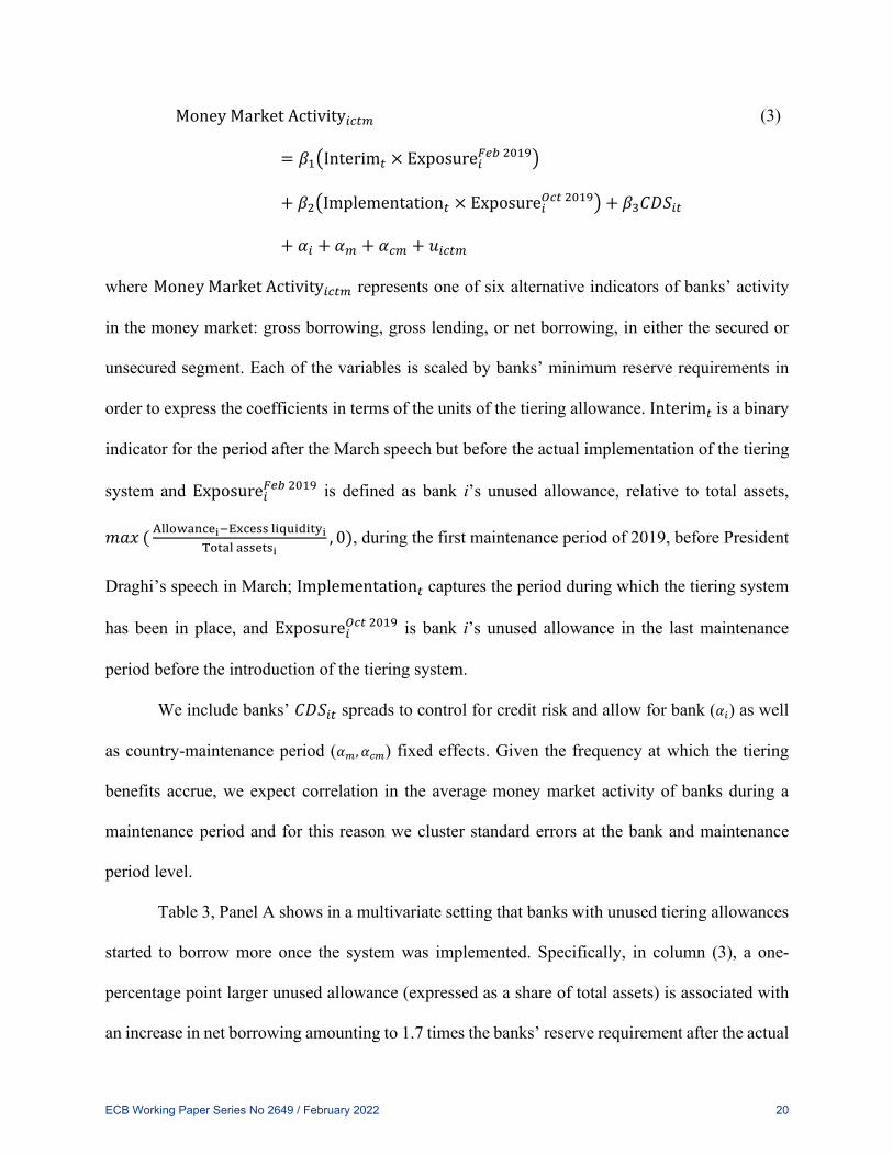
Money Market Activity𝑖𝑖𝑖𝑖𝑡𝑡𝑚𝑚

= 𝛽𝛽1�Interim𝑡𝑡 × Exposure𝑖𝑖𝐹𝐹𝑒𝑒𝐹𝐹 2019�

+ 𝛽𝛽2�Implementation𝑡𝑡 × Exposure𝑖𝑖𝑂𝑂𝑖𝑖𝑡𝑡 2019� + 𝛽𝛽3𝐶𝐶𝐷𝐷𝑆𝑆𝑖𝑖𝑡𝑡

+ 𝛼𝛼𝑖𝑖 + 𝛼𝛼𝑚𝑚 + 𝛼𝛼𝑖𝑖𝑚𝑚 + 𝐸𝐸𝑖𝑖𝑖𝑖𝑡𝑡𝑚𝑚

(3)

where Money Market Activity𝑖𝑖𝑖𝑖𝑡𝑡𝑚𝑚 represents one of six alternative indicators of banks’ activity

in the money market: gross borrowing, gross lending, or net borrowing, in either the secured or

unsecured segment. Each of the variables is scaled by banks’ minimum reserve requirements in

order to express the coefficients in terms of the units of the tiering allowance. Interim𝑡𝑡 is a binary

indicator for the period after the March speech but before the actual implementation of the tiering

system and Exposure𝑖𝑖𝐹𝐹𝑒𝑒𝐹𝐹 2019 is defined as bank i’s unused allowance, relative to total assets,

𝑚𝑚𝑚𝑚𝑚𝑚 ( Allowancei−Excess liquidityiTotal assetsi

, 0), during the first maintenance period of 2019, before President

Draghi’s speech in March; Implementation𝑡𝑡 captures the period during which the tiering system

has been in place, and Exposure𝑖𝑖𝑂𝑂𝑖𝑖𝑡𝑡 2019 is bank i’s unused allowance in the last maintenance

period before the introduction of the tiering system.

We include banks’ 𝐶𝐶𝐷𝐷𝑆𝑆𝑖𝑖𝑡𝑡 spreads to control for credit risk and allow for bank (𝛼𝛼𝑖𝑖) as well

as country-maintenance period (𝛼𝛼𝑚𝑚,𝛼𝛼𝑖𝑖𝑚𝑚) fixed effects. Given the frequency at which the tiering

benefits accrue, we expect correlation in the average money market activity of banks during a

maintenance period and for this reason we cluster standard errors at the bank and maintenance

period level.

Table 3, Panel A shows in a multivariate setting that banks with unused tiering allowances

started to borrow more once the system was implemented. Specifically, in column (3), a one-

percentage point larger unused allowance (expressed as a share of total assets) is associated with

an increase in net borrowing amounting to 1.7 times the banks’ reserve requirement after the actual


implementation of the system. We do not observe significant changes in gross borrowing, and the

adjustment in gross lending is significant only at the 10 percent level, indicating that different

banks achieved the desired increased in excess liquidity adjusting on different margins. We

observe no significant changes in net borrowing in the secured market for banks with more unused

allowances during the interim period.

Columns (4)-(6) show that similar developments took place in the unsecured segment of

the euro money market, albeit at somewhat smaller magnitude, in line with the descriptive

evidence in Figure 3.

These effects are economically meaningful. As outlined in section 2.1, each eligible bank

received a tiering allowance exempting excess liquidity holdings up to six times their MRR from

the application of the negative deposit facility rate. The average treatment effect of between 0.7-

1.7 times banks’ MRR thus implies that banks with a one percentage point higher unused

exemption increased their net borrowing in the money market by around one sixth of their total

allowance more than banks without unused allowances. The average treatment effect is also

substantial relative to the stock of outstanding money market transactions during the sample

period, which amount to around 2.2 times MRR in the secured segment and around 7.4 times MRR

in the unsecured segment (see Table 1, panel 3).

These results suggest that following the tiering implementation, banks’ willingness to lend

to counterparties with high excess exemptions increased, thanks to the borrowers’ ability to store

liquidity at a non-negative rate. To be able to interpret these results as driven by an improvement

in banks’ access to the money market we use high-dimensional fixed effects to control for shocks

that may have affected the banks (Khwaja and Mian, 2008).

Panel B controls for the supply of short-term funding by including interactions of lender


(counterparty) and maintenance period fixed effects. The results show that unsecured borrowing

by a bank with more unused exemptions rises significantly more than for a bank without unused

exemptions borrowing from the same counterparty. This suggests that banks exposed to the tiering

system became able to obtain more liquidity than other banks, suggesting that they were

reintegrated in the money market. This finding is robust if we control for characteristics of the

relationships by including interaction between counterparty and lending bank fixed effects or

shocks to the country of the borrowers that may drive the demand for liquidity independently from

the excess exemptions. Specifically, the shocks to the country of the borrower allow us to control

for the fact that demand for corporate credit may have increased in the country of the borrowing

bank contextually to the tiering adoption.

5.4. Excess Liquidity and Bond Holdings

The changes in money market activity are mirrored by changes in the composition of bank

assets. Table 4 explores how banks with different ex ante holdings of excess liquidity change their

holdings of excess liquidity. Expected returns on the holdings of excess liquidity increase when

the possibility of the adoption of a tiering system was announced in March 2019. Thus, banks with

lower liquid holdings and consequently higher expected unused exemptions increase their holdings

of excess liquidity during the period between March and October 2019. A one-standard-deviation

(1.5pp) increase in unused exemptions is associated with an increase in excess liquidity holdings

by close to 12bps of total assets. The increase in holdings of excess liquidity is three times larger

after the tiering system is finally implemented in November 2019.

While, as shown in Table 3, money markets contributed to the reallocation of excess

liquidity in November 2019, also the composition of banks’ assets may have changed.


Table 5 considers banks’ holdings of government securities. Government securities are

often used as collateral to borrow in the money market. We expect them to be particularly high in

periods of high uncertainty. It appears that banks decrease their holdings of government securities

after the implementation of the tiering system, when uncertainty about the ability to obtain liquidity

through the money market abates. Following the implementation of the two-tier system, a one-

standard-deviation increase in a bank’s ex-ante unused allowances is associated with a decrease in

the holdings of government securities by close to 4 basis points of total assets (corresponding to

just under 10% of the standard deviation of this variable).

Finally, Table 6 shows that liquidity is reallocated without any changes in the size of the

balance sheet of banks with different benefits from the exemptions.

6. The Effects of the Tiering System on the Transmission Mechanism

This section concentrates on whether the tiering system can affect the bank-based

transmission of monetary policy. There are several mechanisms through which a tiering system

may matter. First, as we have shown, the introduction of the tiering system affects bank net wealth

and the value of excess liquidity. Specifically, banks with excess liquidity, whose net wealth

improves, may become more inclined to lend. Second, the higher value of excess liquidity may

lead lenders with unused exemptions to extend less credit. Third, the introduction of the tiering

system appears to have improved the functioning of money markets. In this respect, banks whose

access to money markets improves, facing less uncertainty, may become more inclined to lend.

Different mechanisms associated with the introduction of the tiering have different

implications on the effects of excess liquidity on bank lending, when exemptions increase. The net

wealth channel, as well as the channel that goes through the marginal value of excess liquidity,


would imply that the credit supply of banks with high unused exemptions is less affected.

Mechanisms that rely on excess liquidity becoming a “hot potato” in periods with negative rates

would even imply that banks with unused exemptions may become less prone to lend. In contrast,

if an improvement in the functioning of the money market spurs lending, we expect that banks that

were ex ante negatively affected by market segmentations lend more. These relatively financially

constrained banks may presumably have substantial unused tiering allowances.

To evaluate which channels are more relevant, we investigate how the lending policies of

firms with different levels of excess liquidity, and higher unused exemptions in particular, differ

from those of other banks. The granularity of Anacredit, the euro area countries’ harmonised credit

register, allows us to identify the supply of credit by exploring how different banks extend credit

to the same borrower.

Specifically, we estimate the following equation:

𝐸𝐸𝐿𝐿𝑚𝑚𝐿𝐿𝑓𝑓,𝐹𝐹,𝑡𝑡 = 𝛽𝛽1�Interim𝑡𝑡 × Exposure𝑖𝑖𝐹𝐹𝑒𝑒𝐹𝐹 2019�

+ 𝛽𝛽2�Implementation𝑡𝑡 × Exposure𝑖𝑖𝑂𝑂𝑖𝑖𝑡𝑡 2019� + 𝛽𝛽3𝑋𝑋𝐹𝐹,𝑡𝑡 + 𝛾𝛾𝑓𝑓,𝑡𝑡 + 𝛿𝛿𝐹𝐹,𝑓𝑓

+ 𝜀𝜀𝑓𝑓,𝐹𝐹,𝑡𝑡

(4)

where the dependent variable is either the amount of the loan or another loan characteristic that

bank b extends to firm f during month t. The dummy variables 𝐼𝐼𝐿𝐿𝐸𝐸𝐼𝐼𝐼𝐼𝐸𝐸𝑚𝑚𝑡𝑡 and 𝐼𝐼𝑚𝑚𝐼𝐼𝐼𝐼𝐼𝐼𝑚𝑚𝐼𝐼𝐿𝐿𝐸𝐸𝑚𝑚𝐸𝐸𝐸𝐸𝐿𝐿𝐿𝐿𝑡𝑡

capture the different phases of the process that led to the introduction of the tiering. The exposure

variables are defined as the unused exemptions in the months just before the first mentioning of

the tiering in President Draghi’s speech and before the tiering implementation, respectively.

Finally, 𝑋𝑋𝐹𝐹,𝑡𝑡 consists of bank level controls including the bank’s CDS spread, excess liquidity,

holdings of government bonds, deposit ratio, and use of TLTRO funds. Importantly, in the most

stringent specifications, we control for loan demand using interactions of firm and time fixed


effects as well as interactions of bank and firm fixed effects, capturing time-invariant aspects of

the relationships.

Table 7 starts by exploring the different mechanisms through which the introduction of the

tiering may affect banks’ lending policies. Specifically, we run a “horse race” between the

exposure variables capturing the magnitude of a bank’s unused exemptions, with banks’ tiering

savings and excess liquidity. Tiering savings do not appear to affect bank lending policies,

suggesting that the tiering system does not facilitate the transmission of monetary policy through

banks’ wealth effects. Similarly, we find no differences in lending between banks with different

levels of excess liquidity holdings. It rather appears that banks with unused exemptions extend

more credit than other banks to the same borrower after the implementation of the tiering system.

The positive effect of unused exemptions on bank lending suggests that the improvements in the

access to the money market spurs banks’ lending.

Table 8 explores the robustness of this result. The results do not appear to be driven by the

fact that Table 7 identifies differences in lending policies from borrowers with multiple lenders.

Results are qualitatively similar when we absorb shocks to the demand for credit using interactions

of country and time effects in column (1), interactions of industry, location, size and time fixed

effects in column (2), and increase in magnitude when we include interactions of firm and time

fixed effects in column (3). A one-percentage-point increase in exemption allowances (which is

close to a one standard deviation of this variable) corresponds to an increase in loans to firms by

4-7% depending on the fixed-effects included, with the impact decreasing to 1% when accounting

also for the extensive margin of bank lending (in column (5)).

These results confirm that the effect of the tiering system on bank lending is not driven by

the net wealth channel: The effects on profitability that we capture over our sample period may


have a too small effects on banks’ capital buffers to affect lending policies. The findings also do

not support concerns that a higher return of excess liquidity may discourage bank lending and

suggest that banks with unused exemptions benefit from an improved functioning of the money

market. Such an interpretation is also consistent with the finding that the supply of credit by banks

with high unused allowances increased only in November 2019, when the money markets started

to reallocate liquidity.

Table 9 provides more direct evidence on our conjecture that access to the money market

is the driving force of the effects of the tiering. If the positive effect of high unused tiering

allowances on the supply of credit reflected banks’ improved access to the money market in the

post implementation period, the increase in credit supply should be driven by banks that faced

higher borrowing interest rates in the secured money market before the tiering implementation.

This is precisely what we find in columns (1) and (2), in which we split the sample considering

banks with borrowing rates above and below the median. Column (3) confirms that the differences

in lending behaviour of banks with high unused exemptions in the post-implementation period are

statistically significant and depend on the interest rate that banks faced in the money market before

the implementation period.

Column (4) considers a bank’s actual borrowing rates in the month right before the interim

and the implementation periods. A higher ex ante borrowing rate is associated with increased credit

extension only in the post-implementation period, confirming that the reallocation of liquidity

through the money market and banks’ expectations to be able to borrow matter. All banks with

higher borrowing rates lend more on average (columns (4) and (5)), but banks that have higher

borrowing rates and higher unused exemptions lend even more, possibly because they faced more

uncertainty about access to the credit market before the tiering implementation.


Overall, this evidence indicates that the tiering system, by reducing segmentations in the

money market, increases the supply of credit to non-financial corporations.

Table 10 investigates additional aspects of the loan supply. The introduction of the two-

tier system did not appear to have a significant impact on lending rates, suggesting that banks

largely internalised the change in the average remuneration of their liquidity holdings rather than

passing them on to clients. We find, however, that the implementation of the system translated into

an increase in the maturity of bank loans. This is consistent with an improvement of the

transmission mechanism associated with expectations of a prolonged low interest rate

environment, which in turn enabled banks to lengthen the maturity of their loan portfolio, despite

the low margins. The impact is expressed in days, so that every percentage point increase in unused

exemptions translates into 25 days longer loan maturity.

Also with respect to loan maturities and lending rates there are important differences

between banks, depending on their ex ante access to the money market. Tables 11 and 12 show an

increase in loan maturity and a drop in lending rates for banks that faced higher borrowing rates in

the money market in October 2019, before the tiering implementation. These ex ante financially

constrained banks with high unused exemptions not only increased the supply of credit, but also

extended their average loan maturity and decreased loan rates. Banks that faced borrowing rates

below the median in October 2019 and presumably had better access to the money market, if

anything, decreased their loan maturity. Overall, this evidence indicates that the benefits of the

tiering system on the transmission mechanism arise from improved access to the money market.

Finally, columns (1) to (5) of Table 13 show that the increase in the supply of credit by

banks with high unused exemptions were similarly distributed across borrowers with different risk,

size, profitability, and productivity even though firms with high leverage may have benefitted more


(column (4)). Columns (6) to (8) confirm that the positive effects of the tiering system on bank

lending are driven by financially constrained banks, which we capture as banks with low

capitalization, high CDS spreads, or high money market borrowing rates. This is consistent with

our conjecture that an improvement in the functioning of the money market due to the tiering

system decreases financially constrained banks’ precautionary behaviour and expands the supply

of credit.

7. Conclusions

We show that access to the money market matters for bank lending. Tiered reserve

remuneration systems can enhance the gains from trading excess liquidity which, in turn, helps

decrease segmentation in the money market. Overall, by increasing the gains from reallocating

excess liquidity, these systems can help unfreeze money markets and may thus enhance the

monetary policy transmission mechanism.

We highlight these mechanisms in the context of the euro area. The sharp increase in excess

liquidity in the euro area due to the ample monetary policy accommodation following the financial

crisis has led to an increase in the aggregate cost of holding excess liquidity. Coupled with a

negative interest rate policy, this had the potential to put pressure on bank intermediation capacity

with negative consequences for the bank-based transmission of monetary policy. The introduction

of the two-tier system for reserve remuneration in the euro area countered this risk by improving

banks’ net wealth. In addition, it enhanced the transmission mechanism not only by empowering

the removal of non-negativity restrictions on future expected short rates and contributing to

lengthen loan maturity, but mostly because it revived banks’ activity in the money markets. This

in turn decreased banks’ incentives to piling up precautionary liquidity buffers, thus benefitting

the supply of credit to the real economy.


References Acharya, V. V., & Merrouche, O. (2013). Precautionary hoarding of liquidity and interbank

markets: Evidence from the subprime crisis, Review of Finance 17, 107-160. Afonso, G., Kovner, A., & Schoar, A. (2011). Stressed, not frozen: The federal funds market in

the financial crisis, Journal of Finance, 66(4), 1109–1139. Allen, F., Carletti, E., & Gale, D. (2009). Interbank market liquidity and central bank

intervention, Journal of Monetary Economics, 56, 639–652. Altavilla, C., Boucinha, M. and Peydró, J.L. (2018). Monetary policy and bank profitability in

a low interest rate environment, Economic Policy, 33, 533-583. Altavilla, C., Burlon, L., Giannetti, M., and Holton, S. (2021). Is There a Zero Lower Bound?

The Effects of Negative Policy Rates on Banks and Firms, Journal of Financial Economics, Forthcoming.

Bolton, P., Santos, T. and Scheinkman, J. A. (2011). Outside and inside liquidity, Quarterly Journal of Economics 126, 259–321.

Bottero, M., Minoiu, C., Peydró, J.-L., Polo, A., Presbitero, A., and Sette, E. (2019). Negative Monetary Policy Rates and Portfolio Rebalancing: Evidence from Credit Register Data, International Monetary Fund WP/19/44.

Brunnermeier, M. K. and Koby, Y. (2016). The reversal interest rate: An effective lower bound on monetary policy. Working Paper, Princeton University.

Caballero, R. J., & Krishnamurthy, A. (2008). Collective risk management in a flight to quality episode, Journal of Finance 63, 2195–2230.

Chiu, J., Eisenschmidt, J. & Monnet, C. (2020). Relationships in the Interbank Market, Review of Economic Dynamics 35, 170-191.

Corradin, S., Eisenschmidt, J., Hoerova, M., Linzert, T., Schepens, G., and Sigaux, J-D. (2020). Money markets, central bank balance sheet and regulation, ECB Working Paper No. 2483.

Diamond, D. W. and Rajan, R. G. (2011). Fear of fire sales, illiquidity seeking, and credit freezes. Quarterly Journal of Economics, 126 (2), 557-591.

ECB (2021). Euro money market study 2020: Money market trends as observed through MMSR data.

Eggertsson, G. B., Juelsrud, R. E., Summers, L. H. and Wold, E. G. (2019). Negative Nominal Interest Rates and the Bank Lending Channel, NBER Working Paper No. 25416.

Fuster, A., Schelling, T. and P. Towbin. (2021). Tiers of joy? Reserve tiering and bank behavior in a negative-rate environment, Working Papers 2021-10, Swiss National Bank.

Iyer, R., Peydró, J.-L., da-Rocha-Lopes, S. and Schoar, A. (2014). Interbank Liquidity Crunch and the Firm Credit Crunch: Evidence from the 2007–2009 Crisis. Review of Financial Studies, 27(1), 347–372.

Khwaja, A. and Mian, A. (2008). Tracing the Impact of Bank Liquidity Shocks: Evidence from an Emerging Market. American Economic Review, 98(4), 1413-42.

Rogoff, K. (2016). The Curse of Cash. Princeton University Press. Rogoff, K. (2017). Dealing with Monetary Paralysis at the Zero Bound. Journal of Economic

Perspectives 31, 47–66. Sefcik, S. and Thompson, R. (1986). An approach to statistical inference in cross-sectional

models with security abnormal returns as dependent variable. Journal of Accounting Research 24:316–34.

Ulate, M. (2021) Going Negative at the Zero Lower Bound: The Effects of Negative Nominal Interest Rates. American Economic Review, 111 (1): 1-40.


Figures

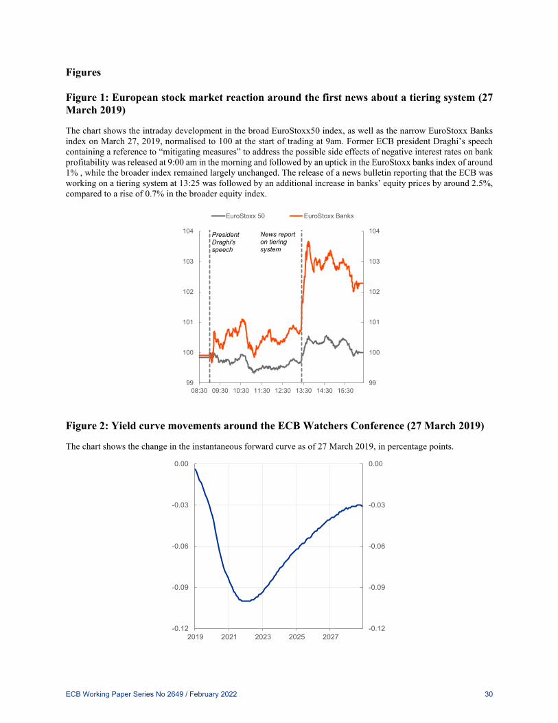
Figure 1: European stock market reaction around the first news about a tiering system (27 March 2019)

The chart shows the intraday development in the broad EuroStoxx50 index, as well as the narrow EuroStoxx Banks index on March 27, 2019, normalised to 100 at the start of trading at 9am. Former ECB president Draghi’s speech containing a reference to “mitigating measures” to address the possible side effects of negative interest rates on bank profitability was released at 9:00 am in the morning and followed by an uptick in the EuroStoxx banks index of around 1% , while the broader index remained largely unchanged. The release of a news bulletin reporting that the ECB was working on a tiering system at 13:25 was followed by an additional increase in banks’ equity prices by around 2.5%, compared to a rise of 0.7% in the broader equity index.

Figure 2: Yield curve movements around the ECB Watchers Conference (27 March 2019)

The chart shows the change in the instantaneous forward curve as of 27 March 2019, in percentage points.

99

100

101

102

103

104

99

100

101

102

103

104

08:30 09:30 10:30 11:30 12:30 13:30 14:30 15:30

EuroStoxx 50 EuroStoxx Banks

PresidentDraghi's speech

News report on tiering system

-0.12

-0.09

-0.06

-0.03

0.00

-0.12

-0.09

-0.06

-0.03

0.00

2019 2021 2023 2025 2027


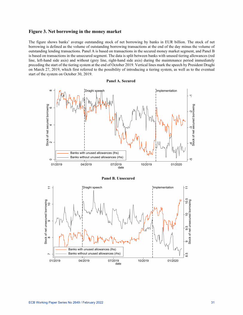
Figure 3. Net borrowing in the money market

The figure shows banks’ average outstanding stock of net borrowing by banks in EUR billion. The stock of net borrowing is defined as the volume of outstanding borrowing transactions at the end of the day minus the volume of outstanding lending transactions. Panel A is based on transactions in the secured money market segment, and Panel B is based on transactions in the unsecured segment. The data is split between banks with unused tiering allowances (red line, left-hand side axis) and without (grey line, right-hand side axis) during the maintenance period immediately preceding the start of the tiering system at the end of October 2019. Vertical lines mark the speech by President Draghi on March 27, 2019, which first referred to the possibility of introducing a tiering system, as well as to the eventual start of the system on October 30, 2019.

Panel A. Secured

Panel B. Unsecured

Draghi speech Implementation

-5-4

-3-2

-1St

ock

of n

et s

ecur

ed b

orro

win

g

02

46

8St

ock

of n

et s

ecur

ed b

orro

win

g

01/2019 04/2019 07/2019 10/2019 01/2020date

Banks with unused allowances (lhs)Banks without unused allowances (rhs)

Draghi speech Implementation8.

59

9.5

1010

.511

Stoc

k of

net

uns

ecur

ed b

orro

win

g

78

910

11St

ock

of n

et u

nsec

ured

bor

row

ing

01/2019 04/2019 07/2019 10/2019 01/2020date

Banks with unused allowances (lhs)Banks without unused allowances (rhs)


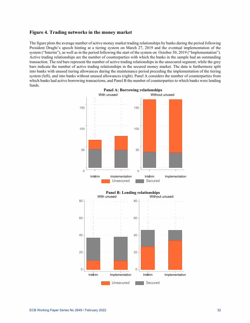
Figure 4. Trading networks in the money market

The figure plots the average number of active money market trading relationships by banks during the period following President Draghi’s speech hinting at a tiering system on March 27, 2019 and the eventual implementation of the system (“Interim”), as well as in the period following the start of the system on October 30, 2019 (“Implementation”). Active trading relationships are the number of counterparties with which the banks in the sample had an outstanding transaction. The red bars represent the number of active trading relationships in the unsecured segment, while the grey bars indicate the number of active trading relationships in the secured money market. The data is furthermore split into banks with unused tiering allowances during the maintenance period preceding the implementation of the tiering system (left), and into banks without unused allowances (right). Panel A considers the number of counterparties from which banks had active borrowing transactions, and Panel B the number of counterparties to which banks were lending funds.

Panel A: Borrowing relationships

Panel B: Lending relationships

0

50

100

150

0

50

100

150

1Interim Implementation 1Interim Implementation

With unused Without unused

Unsecured Secured

0

20

40

60

80

0

20

40

60

80

1Interim Implementation 1Interim Implementation

With unused Without unused

Unsecured Secured


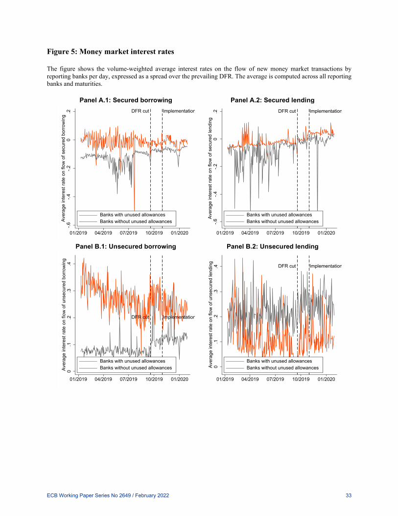
Figure 5: Money market interest rates The figure shows the volume-weighted average interest rates on the flow of new money market transactions by reporting banks per day, expressed as a spread over the prevailing DFR. The average is computed across all reporting banks and maturities.

Panel A.1: Secured borrowing Panel A.2: Secured lending

Panel B.1: Unsecured borrowing Panel B.2: Unsecured lending

DFR cut Implementation

-.6-.4

-.20

.2Av

erag

e in

tere

st ra

te o

n flo

w o

f sec

ured

bor

row

ing

01/2019 04/2019 07/2019 10/2019 01/2020

Banks with unused allowancesBanks without unused allowances


-.6-.4

-.20

.2Av

erag

e in

tere

st ra

te o

n flo

w o

f sec

ured

lend

ing

01/2019 04/2019 07/2019 10/2019 01/2020



0.1

.2.3

.4Av

erag

e in

tere

st ra

te o

n flo

w o

f uns

ecur

ed b

orro

win

g

01/2019 04/2019 07/2019 10/2019 01/2020



0.1

.2.3

.4Av

erag

e in

tere

st ra

te o

n flo

w o

f uns

ecur

ed le

ndin

g

01/2019 04/2019 07/2019 10/2019 01/2020



Tables

Table 1: Summary statistics

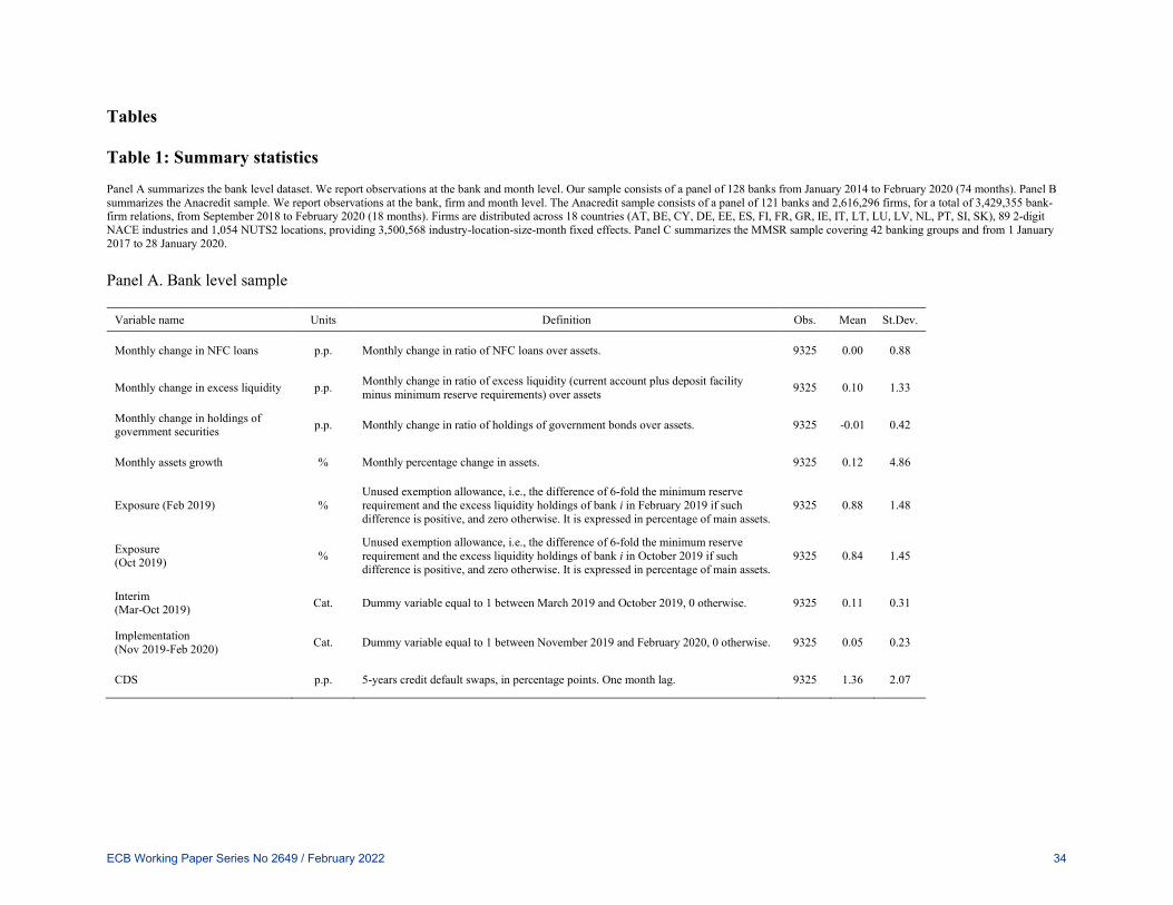
Panel A summarizes the bank level dataset. We report observations at the bank and month level. Our sample consists of a panel of 128 banks from January 2014 to February 2020 (74 months). Panel B summarizes the Anacredit sample. We report observations at the bank, firm and month level. The Anacredit sample consists of a panel of 121 banks and 2,616,296 firms, for a total of 3,429,355 bank-firm relations, from September 2018 to February 2020 (18 months). Firms are distributed across 18 countries (AT, BE, CY, DE, EE, ES, FI, FR, GR, IE, IT, LT, LU, LV, NL, PT, SI, SK), 89 2-digit NACE industries and 1,054 NUTS2 locations, providing 3,500,568 industry-location-size-month fixed effects. Panel C summarizes the MMSR sample covering 42 banking groups and from 1 January 2017 to 28 January 2020. Panel A. Bank level sample

Variable name Units Definition Obs. Mean St.Dev.

Monthly change in NFC loans p.p. Monthly change in ratio of NFC loans over assets. 9325 0.00 0.88

Monthly change in excess liquidity p.p. Monthly change in ratio of excess liquidity (current account plus deposit facility minus minimum reserve requirements) over assets 9325 0.10 1.33

Monthly change in holdings of government securities p.p. Monthly change in ratio of holdings of government bonds over assets. 9325 -0.01 0.42

Monthly assets growth % Monthly percentage change in assets. 9325 0.12 4.86

Exposure (Feb 2019) % Unused exemption allowance, i.e., the difference of 6-fold the minimum reserve requirement and the excess liquidity holdings of bank i in February 2019 if such difference is positive, and zero otherwise. It is expressed in percentage of main assets.

9325 0.88 1.48

Exposure (Oct 2019) %

Unused exemption allowance, i.e., the difference of 6-fold the minimum reserve requirement and the excess liquidity holdings of bank i in October 2019 if such difference is positive, and zero otherwise. It is expressed in percentage of main assets.

9325 0.84 1.45

Interim (Mar-Oct 2019) Cat. Dummy variable equal to 1 between March 2019 and October 2019, 0 otherwise. 9325 0.11 0.31

Implementation (Nov 2019-Feb 2020) Cat. Dummy variable equal to 1 between November 2019 and February 2020, 0 otherwise. 9325 0.05 0.23

CDS p.p. 5-years credit default swaps, in percentage points. One month lag. 9325 1.36 2.07


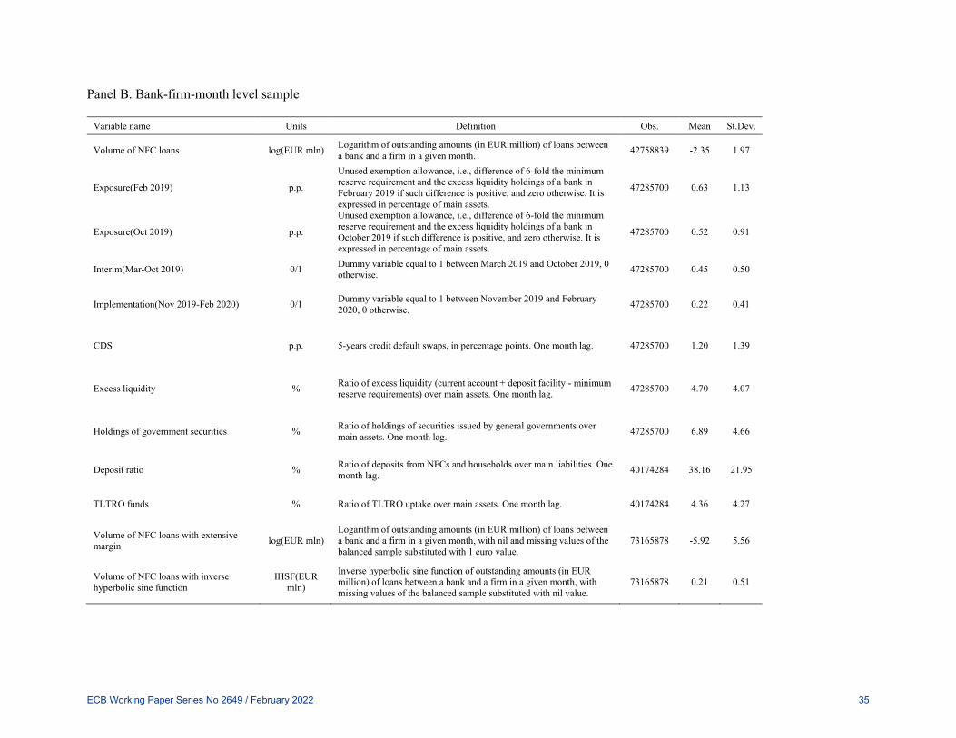
Panel B. Bank-firm-month level sample

Variable name Units Definition Obs. Mean St.Dev.

Volume of NFC loans log(EUR mln) Logarithm of outstanding amounts (in EUR million) of loans between a bank and a firm in a given month. 42758839 -2.35 1.97

Exposure(Feb 2019) p.p.

Unused exemption allowance, i.e., difference of 6-fold the minimum reserve requirement and the excess liquidity holdings of a bank in February 2019 if such difference is positive, and zero otherwise. It is expressed in percentage of main assets.

47285700 0.63 1.13

Exposure(Oct 2019) p.p.

Unused exemption allowance, i.e., difference of 6-fold the minimum reserve requirement and the excess liquidity holdings of a bank in October 2019 if such difference is positive, and zero otherwise. It is expressed in percentage of main assets.

47285700 0.52 0.91

Interim(Mar-Oct 2019) 0/1 Dummy variable equal to 1 between March 2019 and October 2019, 0 otherwise. 47285700 0.45 0.50

Implementation(Nov 2019-Feb 2020) 0/1 Dummy variable equal to 1 between November 2019 and February 2020, 0 otherwise. 47285700 0.22 0.41

CDS p.p. 5-years credit default swaps, in percentage points. One month lag. 47285700 1.20 1.39

Excess liquidity % Ratio of excess liquidity (current account + deposit facility - minimum reserve requirements) over main assets. One month lag. 47285700 4.70 4.07

Holdings of government securities % Ratio of holdings of securities issued by general governments over main assets. One month lag. 47285700 6.89 4.66

Deposit ratio % Ratio of deposits from NFCs and households over main liabilities. One month lag. 40174284 38.16 21.95

TLTRO funds % Ratio of TLTRO uptake over main assets. One month lag. 40174284 4.36 4.27

Volume of NFC loans with extensive margin log(EUR mln)

Logarithm of outstanding amounts (in EUR million) of loans between a bank and a firm in a given month, with nil and missing values of the balanced sample substituted with 1 euro value.

73165878 -5.92 5.56

Volume of NFC loans with inverse hyperbolic sine function

IHSF(EUR mln)

Inverse hyperbolic sine function of outstanding amounts (in EUR million) of loans between a bank and a firm in a given month, with missing values of the balanced sample substituted with nil value.

73165878 0.21 0.51


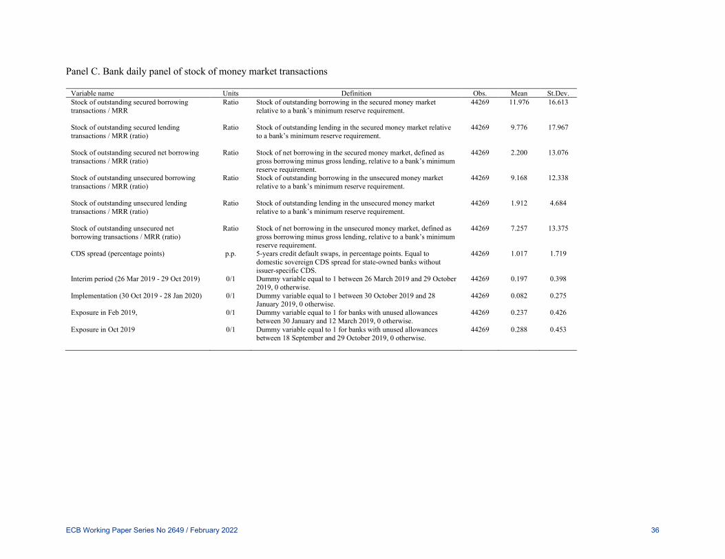
Panel C. Bank daily panel of stock of money market transactions

Variable name Units Definition Obs. Mean St.Dev. Stock of outstanding secured borrowing transactions / MRR

Ratio Stock of outstanding borrowing in the secured money market relative to a bank’s minimum reserve requirement.

44269 11.976 16.613

Stock of outstanding secured lending transactions / MRR (ratio)

Ratio Stock of outstanding lending in the secured money market relative to a bank’s minimum reserve requirement.

44269 9.776 17.967

Stock of outstanding secured net borrowing transactions / MRR (ratio)

Ratio Stock of net borrowing in the secured money market, defined as gross borrowing minus gross lending, relative to a bank’s minimum reserve requirement.

44269 2.200 13.076

Stock of outstanding unsecured borrowing transactions / MRR (ratio)

Ratio Stock of outstanding borrowing in the unsecured money market relative to a bank’s minimum reserve requirement.

44269 9.168 12.338

Stock of outstanding unsecured lending transactions / MRR (ratio)

Ratio Stock of outstanding lending in the unsecured money market relative to a bank’s minimum reserve requirement.

44269 1.912 4.684

Stock of outstanding unsecured net borrowing transactions / MRR (ratio)

Ratio Stock of net borrowing in the unsecured money market, defined as gross borrowing minus gross lending, relative to a bank’s minimum reserve requirement.

44269 7.257 13.375

CDS spread (percentage points)

p.p. 5-years credit default swaps, in percentage points. Equal to domestic sovereign CDS spread for state-owned banks without issuer-specific CDS.

44269 1.017 1.719

Interim period (26 Mar 2019 - 29 Oct 2019)

0/1 Dummy variable equal to 1 between 26 March 2019 and 29 October 2019, 0 otherwise.

44269 0.197 0.398

Implementation (30 Oct 2019 - 28 Jan 2020)

0/1 Dummy variable equal to 1 between 30 October 2019 and 28 January 2019, 0 otherwise.

44269 0.082 0.275

Exposure in Feb 2019, 0/1 Dummy variable equal to 1 for banks with unused allowances between 30 January and 12 March 2019, 0 otherwise.

44269 0.237 0.426

Exposure in Oct 2019

0/1 Dummy variable equal to 1 for banks with unused allowances between 18 September and 29 October 2019, 0 otherwise.

44269 0.288 0.453


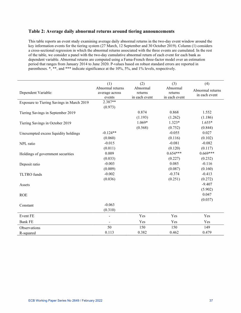
Table 2: Average daily abnormal returns around tiering announcements This table reports an event study examining average daily abnormal returns in the two-day event window around the key information events for the tiering system (27 March, 12 September and 30 October 2019). Column (1) considers a cross-sectional regression in which the abnormal returns associated with the three events are cumulated. In the rest of the table, we consider a panel with the two-day cumulative abnormal return of each event for each bank as dependent variable. Abnormal returns are computed using a Fama-French three-factor model over an estimation period that ranges from January 2014 to June 2020. P-values based on robust standard errors are reported in parentheses. *, **, and *** indicate significance at the 10%, 5%, and 1% levels, respectively.

(1) (2) (3) (4)

Dependent Variable: Abnormal returns

average across events

Abnormal returns

in each event

Abnormal returns

in each event

Abnormal returns in each event

Exposure to Tiering Savings in March 2019 2.387**

(0.973)

Tiering Savings in September 2019

0.874 0.868 1.552

(1.193) (1.262) (1.186)

Tiering Savings in October 2019

1.069* 1.323* 1.655*

(0.568) (0.752) (0.844)

Unexempted excess liquidity holdings -0.124**

-0.055 0.027 (0.060)

(0.116) (0.102)

NPL ratio -0.015

-0.081 -0.082 (0.011)

(0.120) (0.117)

Holdings of government securities 0.009

0.654*** 0.669*** (0.033)

(0.227) (0.232)

Deposit ratio -0.003

0.085 -0.116 (0.009)

(0.087) (0.160)

TLTRO funds -0.002

-0.374 -0.413 (0.036)

(0.251) (0.272)

Assets

-9.407

(5.902)

ROE

0.047

(0.037)

Constant -0.063

(0.310)

Event FE - Yes Yes Yes Bank FE - Yes Yes Yes Observations 50 150 150 149 R-squared 0.113 0.382 0.462 0.479


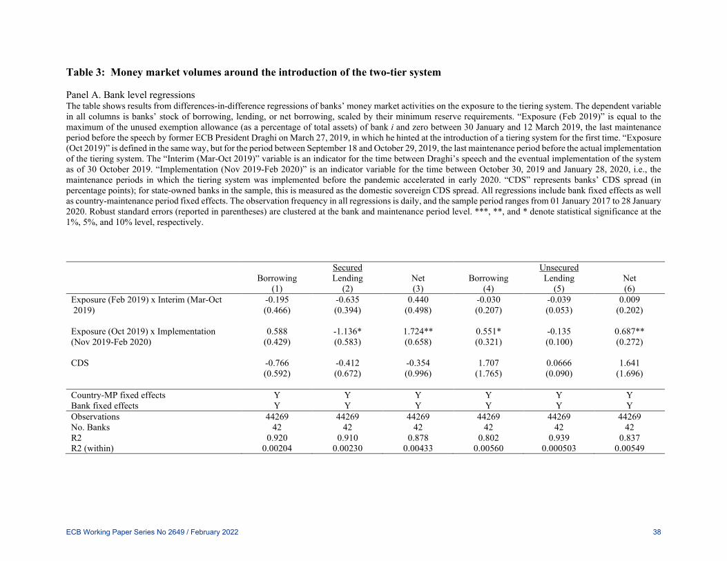
Table 3: Money market volumes around the introduction of the two-tier system Panel A. Bank level regressions The table shows results from differences-in-difference regressions of banks’ money market activities on the exposure to the tiering system. The dependent variable in all columns is banks’ stock of borrowing, lending, or net borrowing, scaled by their minimum reserve requirements. “Exposure (Feb 2019)” is equal to the maximum of the unused exemption allowance (as a percentage of total assets) of bank i and zero between 30 January and 12 March 2019, the last maintenance period before the speech by former ECB President Draghi on March 27, 2019, in which he hinted at the introduction of a tiering system for the first time. “Exposure (Oct 2019)” is defined in the same way, but for the period between September 18 and October 29, 2019, the last maintenance period before the actual implementation of the tiering system. The “Interim (Mar-Oct 2019)” variable is an indicator for the time between Draghi’s speech and the eventual implementation of the system as of 30 October 2019. “Implementation (Nov 2019-Feb 2020)” is an indicator variable for the time between October 30, 2019 and January 28, 2020, i.e., the maintenance periods in which the tiering system was implemented before the pandemic accelerated in early 2020. “CDS” represents banks’ CDS spread (in percentage points); for state-owned banks in the sample, this is measured as the domestic sovereign CDS spread. All regressions include bank fixed effects as well as country-maintenance period fixed effects. The observation frequency in all regressions is daily, and the sample period ranges from 01 January 2017 to 28 January 2020. Robust standard errors (reported in parentheses) are clustered at the bank and maintenance period level. ***, **, and * denote statistical significance at the 1%, 5%, and 10% level, respectively.

Secured Unsecured Borrowing Lending Net Borrowing Lending Net (1) (2) (3) (4) (5) (6) Exposure (Feb 2019) x Interim (Mar-Oct -0.195 -0.635 0.440 -0.030 -0.039 0.009 2019)

(0.466) (0.394) (0.498) (0.207) (0.053) (0.202)

Exposure (Oct 2019) x Implementation 0.588 -1.136* 1.724** 0.551* -0.135 0.687** (Nov 2019-Feb 2020)

(0.429) (0.583) (0.658) (0.321) (0.100) (0.272)

CDS -0.766 -0.412 -0.354 1.707 0.0666 1.641

(0.592) (0.672) (0.996) (1.765) (0.090) (1.696)

Country-MP fixed effects Y Y Y Y Y Y Bank fixed effects Y Y Y Y Y Y Observations 44269 44269 44269 44269 44269 44269 No. Banks 42 42 42 42 42 42 R2 0.920 0.910 0.878 0.802 0.939 0.837 R2 (within) 0.00204 0.00230 0.00433 0.00560 0.000503 0.00549


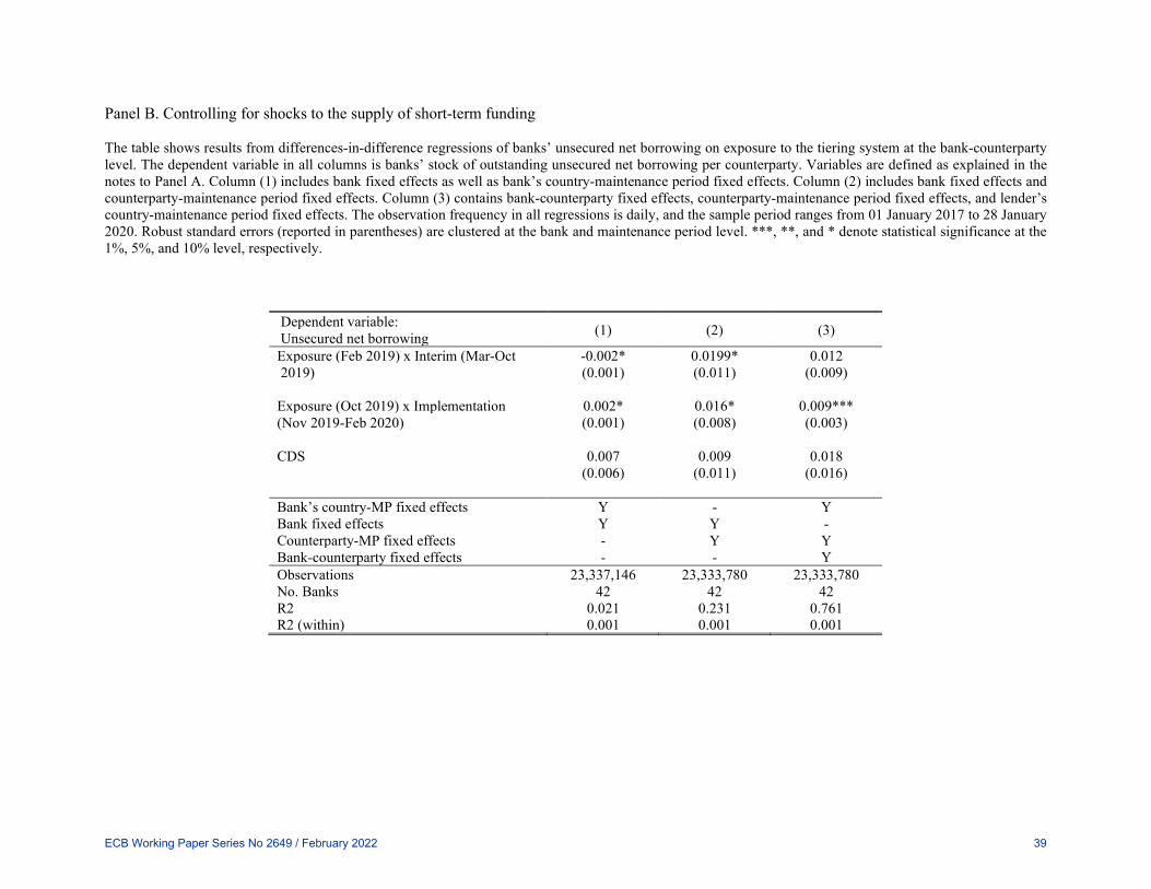
Panel B. Controlling for shocks to the supply of short-term funding The table shows results from differences-in-difference regressions of banks’ unsecured net borrowing on exposure to the tiering system at the bank-counterparty level. The dependent variable in all columns is banks’ stock of outstanding unsecured net borrowing per counterparty. Variables are defined as explained in the notes to Panel A. Column (1) includes bank fixed effects as well as bank’s country-maintenance period fixed effects. Column (2) includes bank fixed effects and counterparty-maintenance period fixed effects. Column (3) contains bank-counterparty fixed effects, counterparty-maintenance period fixed effects, and lender’s country-maintenance period fixed effects. The observation frequency in all regressions is daily, and the sample period ranges from 01 January 2017 to 28 January 2020. Robust standard errors (reported in parentheses) are clustered at the bank and maintenance period level. ***, **, and * denote statistical significance at the 1%, 5%, and 10% level, respectively.

Dependent variable: (1) (2) (3) Unsecured net borrowing Exposure (Feb 2019) x Interim (Mar-Oct -0.002* 0.0199* 0.012 2019)

(0.001) (0.011) (0.009)

Exposure (Oct 2019) x Implementation 0.002* 0.016* 0.009*** (Nov 2019-Feb 2020)

(0.001) (0.008) (0.003)

CDS 0.007 0.009 0.018

(0.006) (0.011) (0.016)

Bank’s country-MP fixed effects Y - Y Bank fixed effects Y Y - Counterparty-MP fixed effects - Y Y Bank-counterparty fixed effects - - Y Observations 23,337,146 23,333,780 23,333,780 No. Banks 42 42 42 R2 0.021 0.231 0.761 R2 (within) 0.001 0.001 0.001


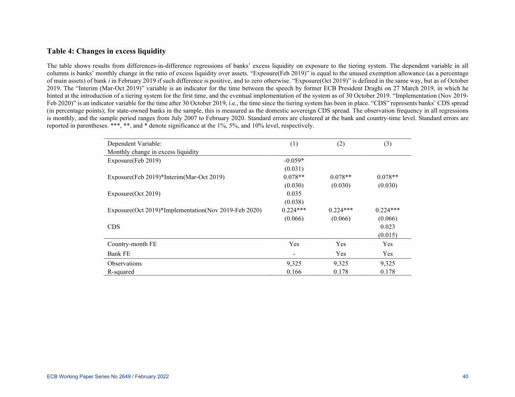
Table 4: Changes in excess liquidity

The table shows results from differences-in-difference regressions of banks’ excess liquidity on exposure to the tiering system. The dependent variable in all columns is banks’ monthly change in the ratio of excess liquidity over assets. “Exposure(Feb 2019)” is equal to the unused exemption allowance (as a percentage of main assets) of bank i in February 2019 if such difference is positive, and to zero otherwise. “Exposure(Oct 2019)” is defined in the same way, but as of October 2019. The “Interim (Mar-Oct 2019)” variable is an indicator for the time between the speech by former ECB President Draghi on 27 March 2019, in which he hinted at the introduction of a tiering system for the first time, and the eventual implementation of the system as of 30 October 2019. “Implementation (Nov 2019-Feb 2020)” is an indicator variable for the time after 30 October 2019, i.e., the time since the tiering system has been in place. “CDS” represents banks’ CDS spread (in percentage points); for state-owned banks in the sample, this is measured as the domestic sovereign CDS spread. The observation frequency in all regressions is monthly, and the sample period ranges from July 2007 to February 2020. Standard errors are clustered at the bank and country-time level. Standard errors are reported in parentheses. ***, **, and * denote significance at the 1%, 5%, and 10% level, respectively.

Dependent Variable: (1) (2) (3) Monthly change in excess liquidity Exposure(Feb 2019) -0.059* (0.031) Exposure(Feb 2019)*Interim(Mar-Oct 2019) 0.078** 0.078** 0.078** (0.030) (0.030) (0.030) Exposure(Oct 2019) 0.035 (0.038) Exposure(Oct 2019)*Implementation(Nov 2019-Feb 2020) 0.224*** 0.224*** 0.224*** (0.066) (0.066) (0.066) CDS 0.023 (0.015) Country-month FE Yes Yes Yes Bank FE - Yes Yes Observations 9,325 9,325 9,325 R-squared 0.166 0.178 0.178


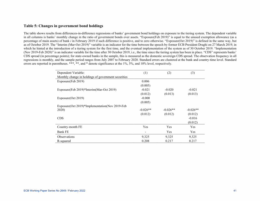
Table 5: Changes in government bond holdings

The table shows results from differences-in-difference regressions of banks’ government bond holdings on exposure to the tiering system. The dependent variable in all columns is banks’ monthly change in the ratio of government bonds over assets. “Exposure(Feb 2019)” is equal to the unused exemption allowance (as a percentage of main assets) of bank i in February 2019 if such difference is positive, and to zero otherwise. “Exposure(Oct 2019)” is defined in the same way, but as of October 2019. The “Interim (Mar-Oct 2019)” variable is an indicator for the time between the speech by former ECB President Draghi on 27 March 2019, in which he hinted at the introduction of a tiering system for the first time, and the eventual implementation of the system as of 30 October 2019. “Implementation (Nov 2019-Feb 2020)” is an indicator variable for the time after 30 October 2019, i.e., the time since the tiering system has been in place. “CDS” represents banks’ CDS spread (in percentage points); for state-owned banks in the sample, this is measured as the domestic sovereign CDS spread. The observation frequency in all regressions is monthly, and the sample period ranges from July 2007 to February 2020. Standard errors are clustered at the bank and country-time level. Standard errors are reported in parentheses. ***, **, and * denote significance at the 1%, 5%, and 10% level, respectively.

Dependent Variable: (1) (2) (3) Monthly change in holdings of government securities Exposure(Feb 2019) 0.006 (0.005) Exposure(Feb 2019)*Interim(Mar-Oct 2019) -0.021 -0.020 -0.021 (0.012) (0.013) (0.013) Exposure(Oct 2019) -0.000 (0.005) Exposure(Oct 2019)*Implementation(Nov 2019-Feb 2020) -0.026** -0.026** -0.026** (0.012) (0.012) (0.012) CDS -0.016 (0.012) Country-month FE Yes Yes Yes Bank FE - Yes Yes Observations 9,325 9,325 9,325 R-squared 0.208 0.217 0.217


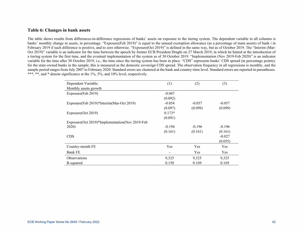
Table 6: Changes in bank assets

The table shows results from differences-in-difference regressions of banks’ assets on exposure to the tiering system. The dependent variable in all columns is banks’ monthly change in assets, in percentage. “Exposure(Feb 2019)” is equal to the unused exemption allowance (as a percentage of main assets) of bank i in February 2019 if such difference is positive, and to zero otherwise. “Exposure(Oct 2019)” is defined in the same way, but as of October 2019. The “Interim (Mar-Oct 2019)” variable is an indicator for the time between the speech by former ECB President Draghi on 27 March 2019, in which he hinted at the introduction of a tiering system for the first time, and the eventual implementation of the system as of 30 October 2019. “Implementation (Nov 2019-Feb 2020)” is an indicator variable for the time after 30 October 2019, i.e., the time since the tiering system has been in place. “CDS” represents banks’ CDS spread (in percentage points); for the state-owned banks in the sample, this is measured as the domestic sovereign CDS spread. The observation frequency in all regressions is monthly, and the sample period ranges from July 2007 to February 2020. Standard errors are clustered at the bank and country-time level. Standard errors are reported in parentheses. ***, **, and * denote significance at the 1%, 5%, and 10% level, respectively.

Dependent Variable: (1) (2) (3) Monthly assets growth Exposure(Feb 2019) -0.047 (0.092) Exposure(Feb 2019)*Interim(Mar-Oct 2019) -0.054 -0.057 -0.057 (0.097) (0.099) (0.099) Exposure(Oct 2019) 0.173* (0.091) Exposure(Oct 2019)*Implementation(Nov 2019-Feb 2020) -0.194 -0.196 -0.196 (0.161) (0.161) (0.161) CDS -0.027 (0.055) Country-month FE Yes Yes Yes Bank FE - Yes Yes Observations 9,325 9,325 9,325 R-squared 0.150 0.169 0.169


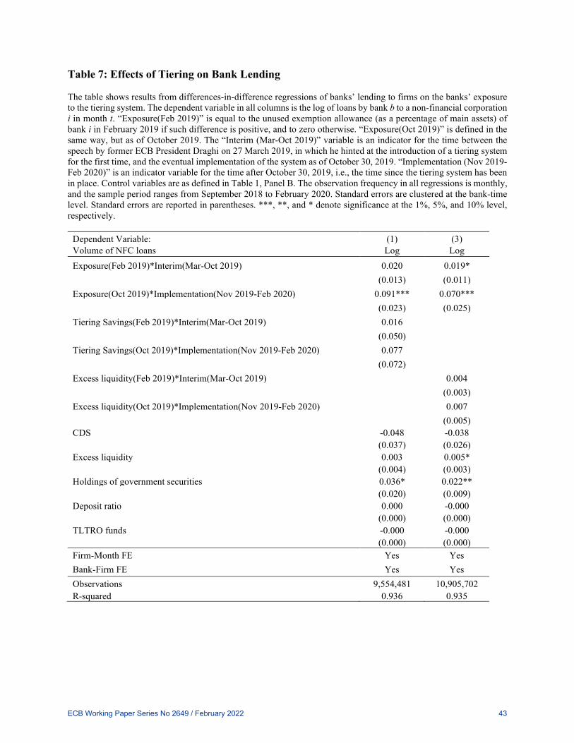
Table 7: Effects of Tiering on Bank Lending The table shows results from differences-in-difference regressions of banks’ lending to firms on the banks’ exposure to the tiering system. The dependent variable in all columns is the log of loans by bank b to a non-financial corporation i in month t. “Exposure(Feb 2019)” is equal to the unused exemption allowance (as a percentage of main assets) of bank i in February 2019 if such difference is positive, and to zero otherwise. “Exposure(Oct 2019)” is defined in the same way, but as of October 2019. The “Interim (Mar-Oct 2019)” variable is an indicator for the time between the speech by former ECB President Draghi on 27 March 2019, in which he hinted at the introduction of a tiering system for the first time, and the eventual implementation of the system as of October 30, 2019. “Implementation (Nov 2019-Feb 2020)” is an indicator variable for the time after October 30, 2019, i.e., the time since the tiering system has been in place. Control variables are as defined in Table 1, Panel B. The observation frequency in all regressions is monthly, and the sample period ranges from September 2018 to February 2020. Standard errors are clustered at the bank-time level. Standard errors are reported in parentheses. ***, **, and * denote significance at the 1%, 5%, and 10% level, respectively.

Dependent Variable: (1) (3) Volume of NFC loans Log Log Exposure(Feb 2019)*Interim(Mar-Oct 2019) 0.020 0.019* (0.013) (0.011) Exposure(Oct 2019)*Implementation(Nov 2019-Feb 2020) 0.091*** 0.070*** (0.023) (0.025) Tiering Savings(Feb 2019)*Interim(Mar-Oct 2019) 0.016 (0.050) Tiering Savings(Oct 2019)*Implementation(Nov 2019-Feb 2020) 0.077 (0.072) Excess liquidity(Feb 2019)*Interim(Mar-Oct 2019) 0.004 (0.003) Excess liquidity(Oct 2019)*Implementation(Nov 2019-Feb 2020) 0.007 (0.005) CDS -0.048 -0.038 (0.037) (0.026) Excess liquidity 0.003 0.005* (0.004) (0.003) Holdings of government securities 0.036* 0.022** (0.020) (0.009) Deposit ratio 0.000 -0.000 (0.000) (0.000) TLTRO funds -0.000 -0.000 (0.000) (0.000) Firm-Month FE Yes Yes Bank-Firm FE Yes Yes Observations 9,554,481 10,905,702 R-squared 0.936 0.935


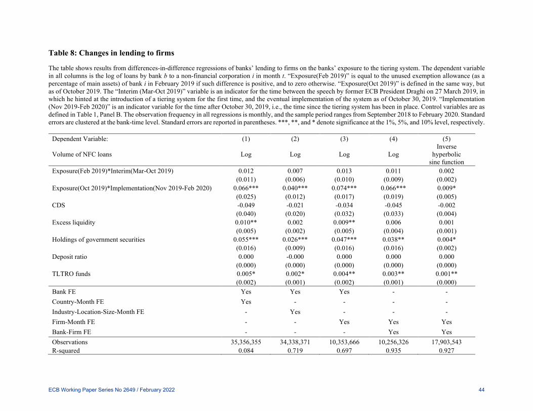
Table 8: Changes in lending to firms

The table shows results from differences-in-difference regressions of banks’ lending to firms on the banks’ exposure to the tiering system. The dependent variable in all columns is the log of loans by bank b to a non-financial corporation i in month t. “Exposure(Feb 2019)” is equal to the unused exemption allowance (as a percentage of main assets) of bank i in February 2019 if such difference is positive, and to zero otherwise. “Exposure(Oct 2019)” is defined in the same way, but as of October 2019. The “Interim (Mar-Oct 2019)” variable is an indicator for the time between the speech by former ECB President Draghi on 27 March 2019, in which he hinted at the introduction of a tiering system for the first time, and the eventual implementation of the system as of October 30, 2019. “Implementation (Nov 2019-Feb 2020)” is an indicator variable for the time after October 30, 2019, i.e., the time since the tiering system has been in place. Control variables are as defined in Table 1, Panel B. The observation frequency in all regressions is monthly, and the sample period ranges from September 2018 to February 2020. Standard errors are clustered at the bank-time level. Standard errors are reported in parentheses. ***, **, and * denote significance at the 1%, 5%, and 10% level, respectively.

Dependent Variable: (1) (2) (3) (4) (5)

Volume of NFC loans Log Log Log Log Inverse

hyperbolic sine function

Exposure(Feb 2019)*Interim(Mar-Oct 2019) 0.012 0.007 0.013 0.011 0.002 (0.011) (0.006) (0.010) (0.009) (0.002) Exposure(Oct 2019)*Implementation(Nov 2019-Feb 2020) 0.066*** 0.040*** 0.074*** 0.066*** 0.009* (0.025) (0.012) (0.017) (0.019) (0.005) CDS -0.049 -0.021 -0.034 -0.045 -0.002 (0.040) (0.020) (0.032) (0.033) (0.004) Excess liquidity 0.010** 0.002 0.009** 0.006 0.001 (0.005) (0.002) (0.005) (0.004) (0.001) Holdings of government securities 0.055*** 0.026*** 0.047*** 0.038** 0.004* (0.016) (0.009) (0.016) (0.016) (0.002) Deposit ratio 0.000 -0.000 0.000 0.000 0.000 (0.000) (0.000) (0.000) (0.000) (0.000) TLTRO funds 0.005* 0.002* 0.004** 0.003** 0.001** (0.002) (0.001) (0.002) (0.001) (0.000) Bank FE Yes Yes Yes - - Country-Month FE Yes - - - - Industry-Location-Size-Month FE - Yes - - - Firm-Month FE - - Yes Yes Yes Bank-Firm FE - - - Yes Yes Observations 35,356,355 34,338,371 10,353,666 10,256,326 17,903,543 R-squared 0.084 0.719 0.697 0.935 0.927


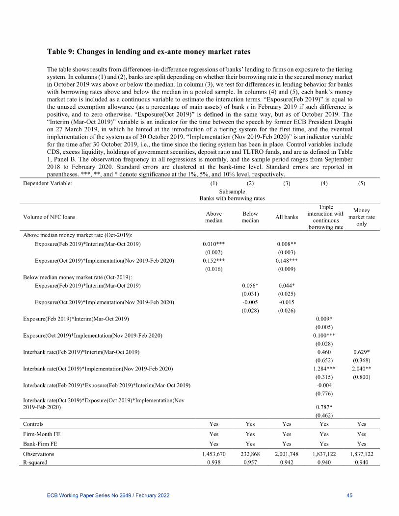
Table 9: Changes in lending and ex-ante money market rates The table shows results from differences-in-difference regressions of banks’ lending to firms on exposure to the tiering system. In columns (1) and (2), banks are split depending on whether their borrowing rate in the secured money market in October 2019 was above or below the median. In column (3), we test for differences in lending behavior for banks with borrowing rates above and below the median in a pooled sample. In columns (4) and (5), each bank’s money market rate is included as a continuous variable to estimate the interaction terms. “Exposure(Feb 2019)” is equal to the unused exemption allowance (as a percentage of main assets) of bank i in February 2019 if such difference is positive, and to zero otherwise. “Exposure(Oct 2019)” is defined in the same way, but as of October 2019. The “Interim (Mar-Oct 2019)” variable is an indicator for the time between the speech by former ECB President Draghi on 27 March 2019, in which he hinted at the introduction of a tiering system for the first time, and the eventual implementation of the system as of 30 October 2019. “Implementation (Nov 2019-Feb 2020)” is an indicator variable for the time after 30 October 2019, i.e., the time since the tiering system has been in place. Control variables include CDS, excess liquidity, holdings of government securities, deposit ratio and TLTRO funds, and are as defined in Table 1, Panel B. The observation frequency in all regressions is monthly, and the sample period ranges from September 2018 to February 2020. Standard errors are clustered at the bank-time level. Standard errors are reported in parentheses. ***, **, and * denote significance at the 1%, 5%, and 10% level, respectively.

Dependent Variable: (1) (2) (3) (4) (5)

Subsample Banks with borrowing rates

Volume of NFC loans Above median

Below median All banks

Triple interaction with

continuous borrowing rate

Money market rate

only

Above median money market rate (Oct-2019): Exposure(Feb 2019)*Interim(Mar-Oct 2019) 0.010*** 0.008** (0.002) (0.003) Exposure(Oct 2019)*Implementation(Nov 2019-Feb 2020) 0.152*** 0.148*** (0.016) (0.009) Below median money market rate (Oct-2019): Exposure(Feb 2019)*Interim(Mar-Oct 2019) 0.056* 0.044* (0.031) (0.025) Exposure(Oct 2019)*Implementation(Nov 2019-Feb 2020) -0.005 -0.015 (0.028) (0.026) Exposure(Feb 2019)*Interim(Mar-Oct 2019) 0.009* (0.005) Exposure(Oct 2019)*Implementation(Nov 2019-Feb 2020) 0.100*** (0.028) Interbank rate(Feb 2019)*Interim(Mar-Oct 2019) 0.460 0.629* (0.652) (0.368) Interbank rate(Oct 2019)*Implementation(Nov 2019-Feb 2020) 1.284*** 2.040** (0.315) (0.800) Interbank rate(Feb 2019)*Exposure(Feb 2019)*Interim(Mar-Oct 2019) -0.004 (0.776) Interbank rate(Oct 2019)*Exposure(Oct 2019)*Implementation(Nov 2019-Feb 2020) 0.787* (0.462) Controls Yes Yes Yes Yes Yes

Firm-Month FE Yes Yes Yes Yes Yes

Bank-Firm FE Yes Yes Yes Yes Yes

Observations 1,453,670 232,868 2,001,748 1,837,122 1,837,122 R-squared 0.938 0.957 0.942 0.940 0.940


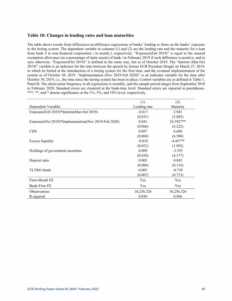
Table 10: Changes in lending rates and loan maturities The table shows results from differences-in-difference regressions of banks’ lending to firms on the banks’ exposure to the tiering system. The dependent variable in columns (1) and (2) are the lending rate and the maturity for a loan from bank b to non-financial corporation i in month f, respectively. “Exposure(Feb 2019)” is equal to the unused exemption allowance (as a percentage of main assets) of bank i in February 2019 if such difference is positive, and to zero otherwise. “Exposure(Oct 2019)” is defined in the same way, but as of October 2019. The “Interim (Mar-Oct 2019)” variable is an indicator for the time between the speech by former ECB President Draghi on March 27, 2019, in which he hinted at the introduction of a tiering system for the first time, and the eventual implementation of the system as of October 30, 2019. “Implementation (Nov 2019-Feb 2020)” is an indicator variable for the time after October 30, 2019, i.e., the time since the tiering system has been in place. Control variables are as defined in Table 1, Panel B. The observation frequency in all regressions is monthly, and the sample period ranges from September 2018 to February 2020. Standard errors are clustered at the bank-time level. Standard errors are reported in parentheses. ***, **, and * denote significance at the 1%, 5%, and 10% level, respectively.

(1) (2) Dependent Variable: Lending rate Maturity Exposure(Feb 2019)*Interim(Mar-Oct 2019) -0.017 2.942 (0.031) (3.882) Exposure(Oct 2019)*Implementation(Nov 2019-Feb 2020) 0.041 24.592*** (0.066) (6.222) CDS 0.097 6.688 (0.068) (6.500) Excess liquidity -0.010 -4.457** (0.021) (1.892) Holdings of government securities 0.009 -3.555 (0.030) (4.177) Deposit ratio 0.005 0.042 (0.006) (0.116) TLTRO funds 0.005 -0.759 (0.007) (0.713) Firm-Month FE Yes Yes Bank-Firm FE Yes Yes Observations 10,256,326 10,256,326 R-squared 0.849 0.966


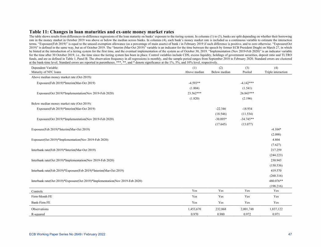
Table 11: Changes in loan maturities and ex-ante money market rates The table shows results from differences-in-difference regressions of the loan maturity on banks’ exposure to the tiering system. In columns (1) to (3), banks are split depending on whether their borrowing rate in the money market in October 2019 was above or below the median across banks. In columns (4), each bank’s money market rate is included as a continuous variable to estimate the interaction terms. “Exposure(Feb 2019)” is equal to the unused exemption allowance (as a percentage of main assets) of bank i in February 2019 if such difference is positive, and to zero otherwise. “Exposure(Oct 2019)” is defined in the same way, but as of October 2019. The “Interim (Mar-Oct 2019)” variable is an indicator for the time between the speech by former ECB President Draghi on March 27, in which he hinted at the introduction of a tiering system for the first time, and the eventual implementation of the system as of October 30, 2019. “Implementation (Nov 2019-Feb 2020)” is an indicator variable for the time after 30 October 2019, i.e., the time since the tiering system has been in place. Control variables include CDS, excess liquidity, holdings of government securities, deposit ratio and TLTRO funds, and are as defined in Table 1, Panel B. The observation frequency in all regressions is monthly, and the sample period ranges from September 2018 to February 2020. Standard errors are clustered at the bank-time level. Standard errors are reported in parentheses. ***, **, and * denote significance at the 1%, 5%, and 10% level, respectively.

Dependent Variable: (1) (2) (3) (4) Maturity of NFC loans Above median Below median Pooled Triple interaction Above median money market rate (Oct-2019):

Exposure(Feb 2019)*Interim(Mar-Oct 2019) -4.593** -4.142*** (1.804) (1.541) Exposure(Oct 2019)*Implementation(Nov 2019-Feb 2020) 23.562*** 26.843*** (1.820) (2.196) Below median money market rate (Oct-2019): Exposure(Feb 2019)*Interim(Mar-Oct 2019) -22.346 -18.934 (18.546) (11.534) Exposure(Oct 2019)*Implementation(Nov 2019-Feb 2020) -30.895* -34.745** (17.645) (13.077) Exposure(Feb 2019)*Interim(Mar-Oct 2019) -4.104* (2.098) Exposure(Oct 2019)*Implementation(Nov 2019-Feb 2020) 4.804 (7.627) Interbank rate(Feb 2019)*Interim(Mar-Oct 2019) 217.259 (244.223) Interbank rate(Oct 2019)*Implementation(Nov 2019-Feb 2020) 230.943 (150.536) Interbank rate(Feb 2019)*Exposure(Feb 2019)*Interim(Mar-Oct 2019) 419.570 (260.316) Interbank rate(Oct 2019)*Exposure(Oct 2019)*Implementation(Nov 2019-Feb 2020) 480.076** (198.216) Controls Yes Yes Yes Yes

Firm-Month FE Yes Yes Yes Yes

Bank-Firm FE Yes Yes Yes Yes

Observations 1,453,670 232,868 2,001,748 1,837,122 R-squared 0.970 0.980 0.972 0.971


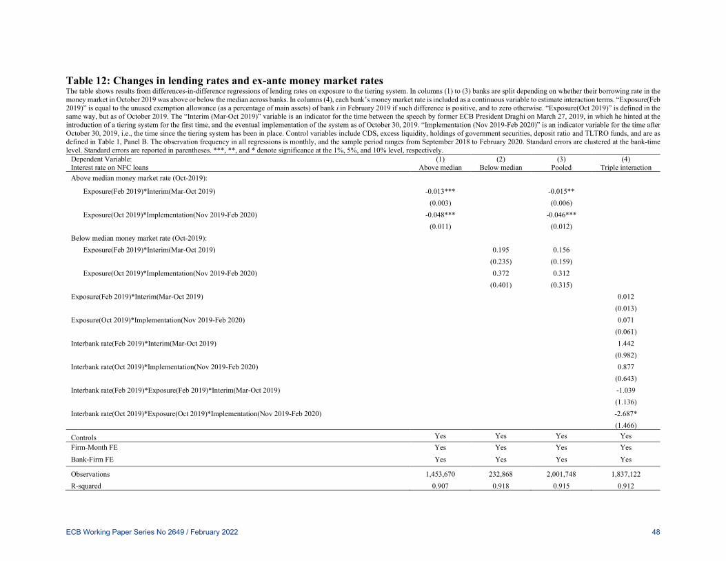
Table 12: Changes in lending rates and ex-ante money market rates The table shows results from differences-in-difference regressions of lending rates on exposure to the tiering system. In columns (1) to (3) banks are split depending on whether their borrowing rate in the money market in October 2019 was above or below the median across banks. In columns (4), each bank’s money market rate is included as a continuous variable to estimate interaction terms. “Exposure(Feb 2019)” is equal to the unused exemption allowance (as a percentage of main assets) of bank i in February 2019 if such difference is positive, and to zero otherwise. “Exposure(Oct 2019)” is defined in the same way, but as of October 2019. The “Interim (Mar-Oct 2019)” variable is an indicator for the time between the speech by former ECB President Draghi on March 27, 2019, in which he hinted at the introduction of a tiering system for the first time, and the eventual implementation of the system as of October 30, 2019. “Implementation (Nov 2019-Feb 2020)” is an indicator variable for the time after October 30, 2019, i.e., the time since the tiering system has been in place. Control variables include CDS, excess liquidity, holdings of government securities, deposit ratio and TLTRO funds, and are as defined in Table 1, Panel B. The observation frequency in all regressions is monthly, and the sample period ranges from September 2018 to February 2020. Standard errors are clustered at the bank-time level. Standard errors are reported in parentheses. ***, **, and * denote significance at the 1%, 5%, and 10% level, respectively.

Dependent Variable: (1) (2) (3) (4) Interest rate on NFC loans Above median Below median Pooled Triple interaction Above median money market rate (Oct-2019):

Exposure(Feb 2019)*Interim(Mar-Oct 2019) -0.013*** -0.015** (0.003) (0.006) Exposure(Oct 2019)*Implementation(Nov 2019-Feb 2020) -0.048*** -0.046*** (0.011) (0.012) Below median money market rate (Oct-2019): Exposure(Feb 2019)*Interim(Mar-Oct 2019) 0.195 0.156 (0.235) (0.159) Exposure(Oct 2019)*Implementation(Nov 2019-Feb 2020) 0.372 0.312 (0.401) (0.315) Exposure(Feb 2019)*Interim(Mar-Oct 2019) 0.012 (0.013) Exposure(Oct 2019)*Implementation(Nov 2019-Feb 2020) 0.071 (0.061) Interbank rate(Feb 2019)*Interim(Mar-Oct 2019) 1.442 (0.982) Interbank rate(Oct 2019)*Implementation(Nov 2019-Feb 2020) 0.877 (0.643) Interbank rate(Feb 2019)*Exposure(Feb 2019)*Interim(Mar-Oct 2019) -1.039 (1.136) Interbank rate(Oct 2019)*Exposure(Oct 2019)*Implementation(Nov 2019-Feb 2020) -2.687* (1.466)

Controls Yes Yes Yes Yes Firm-Month FE Yes Yes Yes Yes Bank-Firm FE Yes Yes Yes Yes

Observations 1,453,670 232,868 2,001,748 1,837,122 R-squared 0.907 0.918 0.915 0.912


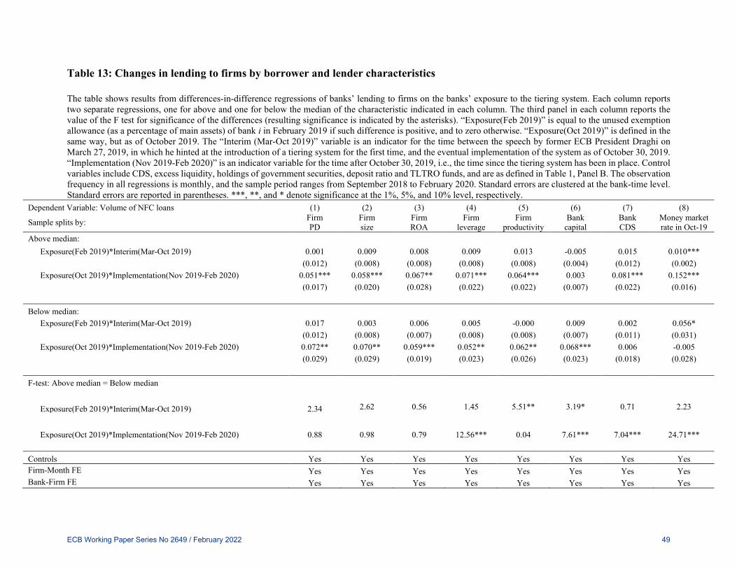
Table 13: Changes in lending to firms by borrower and lender characteristics The table shows results from differences-in-difference regressions of banks’ lending to firms on the banks’ exposure to the tiering system. Each column reports two separate regressions, one for above and one for below the median of the characteristic indicated in each column. The third panel in each column reports the value of the F test for significance of the differences (resulting significance is indicated by the asterisks). “Exposure(Feb 2019)” is equal to the unused exemption allowance (as a percentage of main assets) of bank i in February 2019 if such difference is positive, and to zero otherwise. “Exposure(Oct 2019)” is defined in the same way, but as of October 2019. The “Interim (Mar-Oct 2019)” variable is an indicator for the time between the speech by former ECB President Draghi on March 27, 2019, in which he hinted at the introduction of a tiering system for the first time, and the eventual implementation of the system as of October 30, 2019. “Implementation (Nov 2019-Feb 2020)” is an indicator variable for the time after October 30, 2019, i.e., the time since the tiering system has been in place. Control variables include CDS, excess liquidity, holdings of government securities, deposit ratio and TLTRO funds, and are as defined in Table 1, Panel B. The observation frequency in all regressions is monthly, and the sample period ranges from September 2018 to February 2020. Standard errors are clustered at the bank-time level. Standard errors are reported in parentheses. ***, **, and * denote significance at the 1%, 5%, and 10% level, respectively.

Dependent Variable: Volume of NFC loans (1) (2) (3) (4) (5) (6) (7) (8)

Sample splits by: Firm PD

Firm size

Firm ROA

Firm leverage

Firm productivity

Bank capital

Bank CDS

Money market rate in Oct-19

Above median: Exposure(Feb 2019)*Interim(Mar-Oct 2019) 0.001 0.009 0.008 0.009 0.013 -0.005 0.015 0.010*** (0.012) (0.008) (0.008) (0.008) (0.008) (0.004) (0.012) (0.002) Exposure(Oct 2019)*Implementation(Nov 2019-Feb 2020) 0.051*** 0.058*** 0.067** 0.071*** 0.064*** 0.003 0.081*** 0.152*** (0.017) (0.020) (0.028) (0.022) (0.022) (0.007) (0.022) (0.016) Below median: Exposure(Feb 2019)*Interim(Mar-Oct 2019) 0.017 0.003 0.006 0.005 -0.000 0.009 0.002 0.056* (0.012) (0.008) (0.007) (0.008) (0.008) (0.007) (0.011) (0.031) Exposure(Oct 2019)*Implementation(Nov 2019-Feb 2020) 0.072** 0.070** 0.059*** 0.052** 0.062** 0.068*** 0.006 -0.005 (0.029) (0.029) (0.019) (0.023) (0.026) (0.023) (0.018) (0.028) F-test: Above median = Below median Exposure(Feb 2019)*Interim(Mar-Oct 2019) 2.34 2.62 0.56 1.45 5.51** 3.19* 0.71 2.23

Exposure(Oct 2019)*Implementation(Nov 2019-Feb 2020) 0.88 0.98 0.79 12.56*** 0.04 7.61*** 7.04*** 24.71*** Controls Yes Yes Yes Yes Yes Yes Yes Yes Firm-Month FE Yes Yes Yes Yes Yes Yes Yes Yes Bank-Firm FE Yes Yes Yes Yes Yes Yes Yes Yes


Acknowledgements

We thank seminar participants at the American Economic Association Annual Meeting, the National Bank of Belgium, and the University

of Southampton for comments. Giannetti gratefully acknowledges financial support from the Jan Wallander and Tom Hedelius

Foundation and the Riksbankens Jubileumsfond. Lorenzo Ferrante and Marc Agustí I Torres provided helpful research assistance.

The opinions in this paper are those of the authors and do not necessarily reflect the views of the European Central Bank or the

Eurosystem.

Carlo Altavilla

European Central Bank, Frankfurt am Main, Germany; email: [email protected]

Miguel Boucinha


Lorenzo Burlon


Mariassunta Giannetti

Stockholm School of Economics, Stockholm, Sweden; Centre for Economic Policy Research, London, United Kingdom;

European Corporate Governance Institute, Brussels, Belgium; email: [email protected]

Julian Schumacher


© European Central Bank, 2022

Postal address 60640 Frankfurt am Main, Germany

Telephone +49 69 1344 0

Website www.ecb.europa.eu

All rights reserved. Any reproduction, publication and reprint in the form of a different publication, whether printed or produced

electronically, in whole or in part, is permitted only with the explicit written authorisation of the ECB or the authors.

This paper can be downloaded without charge from www.ecb.europa.eu, from the Social Science Research Network electronic library or

from RePEc: Research Papers in Economics. Information on all of the papers published in the ECB Working Paper Series can be found

on the ECB’s website.

PDF ISBN 978-92-899-4982-8 ISSN 1725-2806 doi: 10.2866/217582 QB-AR-22-014-EN-N

mailto:[email protected]





http://www.ecb.europa.eu/

http://www.ecb.europa.eu/

http://ssrn.com/

https://ideas.repec.org/s/ecb/ecbwps.html

http://www.ecb.europa.eu/pub/research/working-papers/html/index.en.html

Documents

Money markets and bank lending: evidence from the adoption