Monitoring Shear Behavior of Prestressed Concrete Bridge

Delft University of Technology

Monitoring Shear Behavior of Prestressed Concrete Bridge Girders Using AcousticEmission and Digital Image Correlation

Zhang, Fengqiao; Zarate Garnica, Gabriela I.; Yang, Yuguang; Lantsoght, Eva; Sliedrecht, Henk

DOI10.3390/s20195622Publication date2020Document VersionFinal published versionPublished inSensors

Citation (APA)Zhang, F., Zarate Garnica, G. I., Yang, Y., Lantsoght, E., & Sliedrecht, H. (2020). Monitoring ShearBehavior of Prestressed Concrete Bridge Girders Using Acoustic Emission and Digital Image Correlation.Sensors, 20(19), 1-21. [5622]. https://doi.org/10.3390/s20195622

Important noteTo cite this publication, please use the final published version (if applicable).Please check the document version above.

CopyrightOther than for strictly personal use, it is not permitted to download, forward or distribute the text or part of it, without the consentof the author(s) and/or copyright holder(s), unless the work is under an open content license such as Creative Commons.

Takedown policyPlease contact us and provide details if you believe this document breaches copyrights.We will remove access to the work immediately and investigate your claim.

This work is downloaded from Delft University of Technology.For technical reasons the number of authors shown on this cover page is limited to a maximum of 10.

https://doi.org/10.3390/s20195622

https://doi.org/10.3390/s20195622

sensors

Article

Monitoring Shear Behavior of Prestressed ConcreteBridge Girders Using Acoustic Emission and DigitalImage Correlation

Fengqiao Zhang 1,* , Gabriela I. Zarate Garnica 1 , Yuguang Yang 1, Eva Lantsoght 1,2

and Henk Sliedrecht 3

1 Department of Engineering Structures, Delft University of Technology, 2628 CN Delft, The Netherlands;[email protected] (G.I.Z.G.); [email protected] (Y.Y.); [email protected] (E.L.)

2 Politécnico, Universidad San Francisco de Quito, Quito EC 17015, Ecuador3 Rijkswaterstaat, Ministry of Infrastructure and Water Management, 3526 LA Utrecht, The Netherlands;

[email protected]* Correspondence: [email protected]

Received: 25 August 2020; Accepted: 28 September 2020; Published: 1 October 2020��

Abstract: In the Netherlands, many prestressed concrete bridge girders are found to have insufficientshear–tension capacity. We tested four girders taken from a demolished bridge and instrumentedthese with traditional displacement sensors and acoustic emission (AE) sensors, and used cameras fordigital image correlation (DIC). The results show that AE can detect cracking before the traditionaldisplacement sensors, and DIC can identify the cracks with detailed crack kinematics. Both AEand DIC methods provide additional information for the structural analysis, as compared to theconventional measurements: more accurate cracking load, the contribution of aggregate interlock,and the angle of the compression field. These results suggest that both AE and DIC are suitableoptions that warrant further research on their use in lab tests and field testing of prestressed bridges.

Keywords: acoustic emission measurements; crack identification; cracking; digital image correlation;prestressed concrete bridge girders; shear

1. Introduction

Many bridges in the Netherlands were built in the 1960s and 1970s. These bridges were designedfor lower live loads using past code provisions, which may lead to insufficient capacities when assessedwith the current code provisions. Upon assessment, many prestressed concrete bridge girders arereported to have insufficient shear–tension capacity [1,2] according to NEN-EN 1992-1-1:2005 [3].To investigate the actual shear behavior of the existing prestressed concrete girders, four girders weretaken from a typical demolished concrete girder bridge (the Helperzoom bridge) in the Netherlands.Shear tests were performed on these specimens in the Stevin II Laboratory at Delft University ofTechnology. The experimental program was reported in [4], which proved additional capacity comparedto the code provisions [5]. In addition to the conventional measurement techniques, we carried outAcoustic Emission (AE) measurements and photographs were captured during the shear tests forDigital Image Correlation (DIC). These measurements provided additional insights into the structuralbehavior during the cracking and shear failure process.

AE represents the elastic waves excited by sudden changes in the concrete, such as cracking.By continuously recording and processing the AE signals, one can detect the damage process duringloading and unloading. An AE event includes a group of signals that come from one source.With sufficient accuracy [6], one can find the crack profile by locating the source of AE events based onthe arrival times of signals, which is called AE source localization [7]. Besides, features of AE signals

Sensors 2020, 20, 5622; doi:10.3390/s20195622 www.mdpi.com/journal/sensors

http://www.mdpi.com/journal/sensors

http://www.mdpi.com

https://orcid.org/0000-0001-9025-3252

https://orcid.org/0000-0003-3920-0838

https://orcid.org/0000-0003-4548-7644

http://www.mdpi.com/1424-8220/20/19/5622?type=check_update&version=1

http://dx.doi.org/10.3390/s20195622

http://www.mdpi.com/journal/sensors

Sensors 2020, 20, 5622 2 of 21

can help classify different sources of AE events, which is called AE source classification [8–10]. Both AEsource localization and classification are implemented in this paper.

DIC is an optical technique for the evaluation of displacements and strains. It is based oncomparison between images taken during the loading of a specimen. The advantages are that DIC isa non-contact measuring technique and provides full-field displacement measurements of an entirespecimen surface. Thus, DIC has been used to investigate the shear-carrying mechanisms in concretemembers without shear reinforcement [11–13], and prestressed concrete structures [14,15], in thelaboratory. However, the application to full-scale concrete elements is still rare [16–18].

This paper interprets the insights from AE and DIC measurements with regard to three elementsthat are considered important for understanding the cracking and shear failure process of prestressedconcrete girders, namely: cracking load, aggregate interlock, and angle of compression field.

The cracking load is important as it can help estimate the working prestressing level ofthe girder [19] which influences the strain distribution in the cross-section and the deflections.With displacement-based measurements, the cracking load could only be detected by checking thechange in stiffness in the load-deflection curve [20]. As cracking is a local phenomenon, which haslimited effect on the global stiffness, the traditional approach is not sensitive. AE, on the other hand,is known to be sensitive to detecting local (micro)cracking, thus giving a more accurate estimation ofthe cracking load and thus the prestressing level.

The study of the contribution of aggregate interlock and the angle of the compression field can helpunderstand the shear-transfer mechanisms of prestressed concrete girders. Aggregate interlock andstirrups are considered as the main contributors to the shear strength of a cracked concrete girder basedon the Modified Compression Field Theory (MCFT) [21], which is the theoretical basis of the AASHTO(American Association of State Highway and Transportation Officials) shear provisions [22], and thefib Model Code 2010 [23]. According to the aggregate interlock theory of Walraven [24], the shear forcetransfer across cracks through aggregate interlock can be determined once the relative displacementacross the crack trajectory is determined. With the DIC full-field displacement measurement, we candetermine the displacement at any point along the crack to estimate the aggregate interlock and thetensile forces in the stirrups locally.

In plasticity-based models, such as the Variable Angle Truss Model (VATM) [25], a compressionfield is typically used to model the transfer of shear forces in the cracked concrete web of the girder.Such model is employed in NEN-EN 1992-1-1:2005 [3], and is widely accepted in the design ofshear-reinforced concrete elements. This approach idealizes the shear transfer in a cracked memberto a truss model, which has diagonal concrete struts in compression with a variable angle (21.8◦ ≤ θ≤ 45◦). In existing prestressed concrete girders, limited shear reinforcement was applied accordingto the design provisions of that time. As a result, the minimum truss angle defined by the currentcode is often reached for these elements. However, the actual angle of the compression field appearsto be lower than the minimum allowable angle specified by the code provision [5]. DIC providesthe possibility to measure the angle of the compression filed without dense installation of traditionaldisplacement measurements, such as LVDTs (linear variable differential transformers).

The significance of the presented research lies in the additional insights that AE and DIC canprovide in the monitoring of full-scale specimens. This work gives a better understanding of the crackingand shear-carrying behavior of girders in slab-between-girder bridges, and provides recommendationsfor AE and DIC measurements on bridges in the field.

2. Materials and Methods

2.1. Description of Experiments

This section presents the relevant information from the experiments. Additional information onthis series of experiments can be found in a companion paper [4].

Sensors 2020, 20, 5622 3 of 21

2.1.1. Materials and Geometry

The average concrete compressive strength was 76.3 MPa as determined on cores taken from theHelperzoom viaduct, and the splitting tensile strength was 5.4 MPa. The Young’s modulus of theconcrete was 39,548 MPa.

The mild steel (stirrups and longitudinal bars) had a yield strength of 454 MPa and an ultimatestrength of 655 MPa, as determined on material samples in the laboratory. The stirrup ratio was 0.196%.

Samples of the prestressing steel were also tested in the lab. The prestressing steel reached astrain of 0.01 at 1433 MPa and failed at 1824 MPa with a strain of 0.0535. Ten draped tendons with12 strands of 7 mm diameter were used, of which three tendons were anchored in the top flange andthe remaining tendons in the anchorage block.

The total length of the girders was 23.4 m. The girders were cut to about half of their length,varying between 10.51 m and 12.88 m. The resulting four girder segments were numbered consecutivelyas HPZ01 through HPZ04.

2.1.2. Test Setup

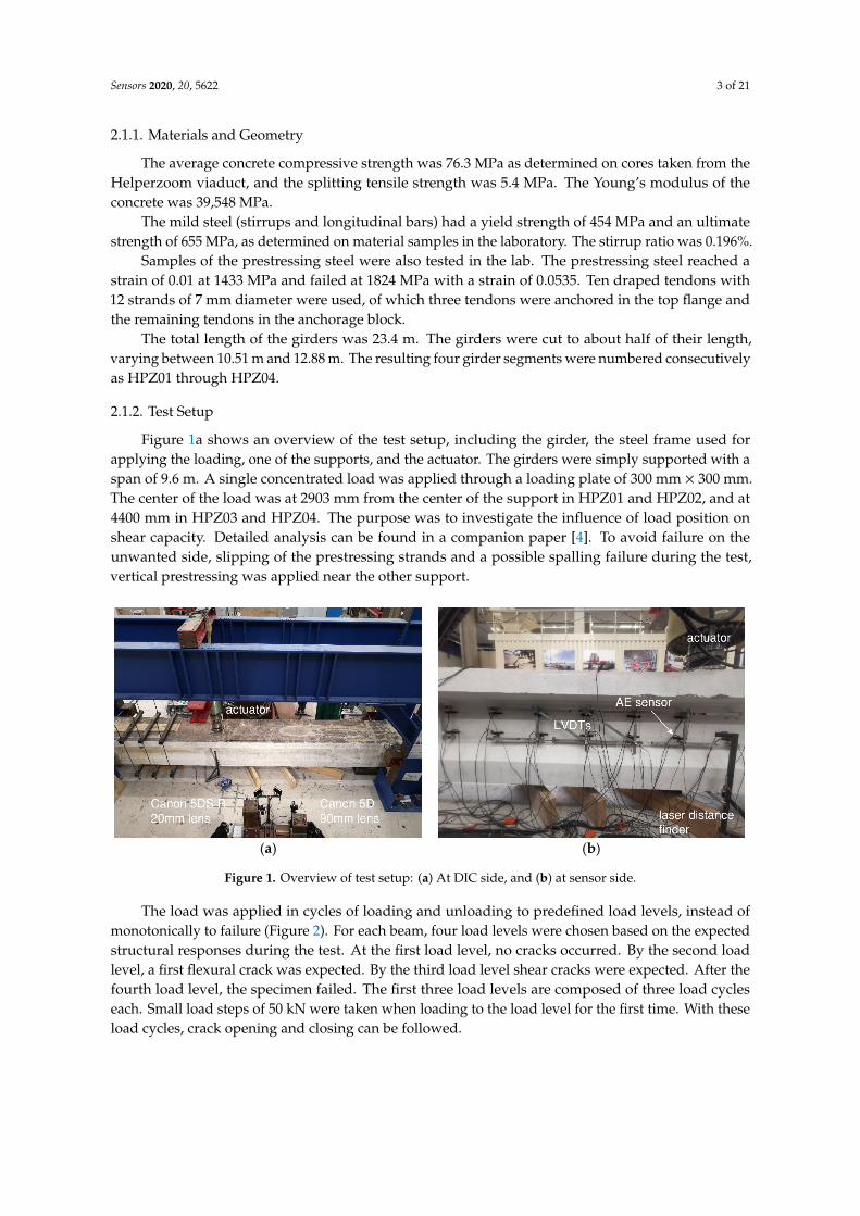
Figure 1a shows an overview of the test setup, including the girder, the steel frame used forapplying the loading, one of the supports, and the actuator. The girders were simply supported with aspan of 9.6 m. A single concentrated load was applied through a loading plate of 300 mm × 300 mm.The center of the load was at 2903 mm from the center of the support in HPZ01 and HPZ02, and at4400 mm in HPZ03 and HPZ04. The purpose was to investigate the influence of load position onshear capacity. Detailed analysis can be found in a companion paper [4]. To avoid failure on theunwanted side, slipping of the prestressing strands and a possible spalling failure during the test,vertical prestressing was applied near the other support.

Sensors 2020, 20, x FOR PEER REVIEW 3 of 21

2.1.1. Materials and Geometry

The average concrete compressive strength was 76.3 MPa as determined on cores taken from the Helperzoom viaduct, and the splitting tensile strength was 5.4 MPa. The Young’s modulus of the concrete was 39,548 MPa.

The mild steel (stirrups and longitudinal bars) had a yield strength of 454 MPa and an ultimate strength of 655 MPa, as determined on material samples in the laboratory. The stirrup ratio was 0.196%.

Samples of the prestressing steel were also tested in the lab. The prestressing steel reached a strain of 0.01 at 1433 MPa and failed at 1824 MPa with a strain of 0.0535. Ten draped tendons with 12 strands of 7 mm diameter were used, of which three tendons were anchored in the top flange and the remaining tendons in the anchorage block.

The total length of the girders was 23.4 m. The girders were cut to about half of their length, varying between 10.51 m and 12.88 m. The resulting four girder segments were numbered consecutively as HPZ01 through HPZ04.

2.1.2. Test Setup

Figure 1a shows an overview of the test setup, including the girder, the steel frame used for applying the loading, one of the supports, and the actuator. The girders were simply supported with a span of 9.6 m. A single concentrated load was applied through a loading plate of 300 mm × 300 mm. The center of the load was at 2903 mm from the center of the support in HPZ01 and HPZ02, and at 4400 mm in HPZ03 and HPZ04. The purpose was to investigate the influence of load position on shear capacity. Detailed analysis can be found in a companion paper [4]. To avoid failure on the unwanted side, slipping of the prestressing strands and a possible spalling failure during the test, vertical prestressing was applied near the other support.

(a) (b)

Figure 1. Overview of test setup: (a) At DIC side, and (b) at sensor side.

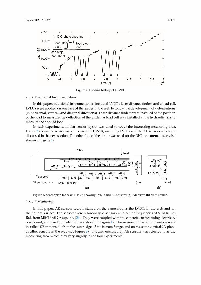
The load was applied in cycles of loading and unloading to predefined load levels, instead of monotonically to failure (Figure 2). For each beam, four load levels were chosen based on the expected structural responses during the test. At the first load level, no cracks occurred. By the second load level, a first flexural crack was expected. By the third load level shear cracks were expected. After the fourth load level, the specimen failed. The first three load levels are composed of three load cycles each. Small load steps of 50 kN were taken when loading to the load level for the first time. With these load cycles, crack opening and closing can be followed.

Figure 1. Overview of test setup: (a) At DIC side, and (b) at sensor side.

The load was applied in cycles of loading and unloading to predefined load levels, instead ofmonotonically to failure (Figure 2). For each beam, four load levels were chosen based on the expectedstructural responses during the test. At the first load level, no cracks occurred. By the second loadlevel, a first flexural crack was expected. By the third load level shear cracks were expected. After thefourth load level, the specimen failed. The first three load levels are composed of three load cycleseach. Small load steps of 50 kN were taken when loading to the load level for the first time. With theseload cycles, crack opening and closing can be followed.

Sensors 2020, 20, 5622 4 of 21Sensors 2020, 20, x FOR PEER REVIEW 4 of 21

Figure 2. Loading history of HPZ04.

2.1.3. Traditional Instrumentation

In this paper, traditional instrumentation included LVDTs, laser distance finders and a load cell. LVDTs were applied on one face of the girder in the web to follow the development of deformations (in horizontal, vertical, and diagonal directions). Laser distance finders were installed at the position of the load to measure the deflection of the girder. A load cell was installed at the hydraulic jack to measure the applied load.

In each experiment, similar sensor layout was used to cover the interesting measuring area. Figure 3 shows the sensor layout as used for HPZ04, including LVDTs and the AE sensors which are discussed in the next section. The other face of the girder was used for the DIC measurements, as also shown in Figure 1a.

(a) (b)

Figure 3. Sensor plan for beam HPZ04 showing LVDTs and AE sensors: (a) Side view; (b) cross-section.

2.2. AE Monitoring

In this paper, AE sensors were installed on the same side as the LVDTs in the web and on the bottom surface. The sensors were resonant type sensors with center frequencies of 60 kHz, i.e., R6I, from MISTRAS Group, Inc. [26]. They were coupled with the concrete surface using electricity compound, and fixed by metal holders, shown in Figure 4a. The sensors on the bottom surface were installed 175 mm inside from the outer edge of the bottom flange, and on the same vertical 2D plane as other sensors in the web (see Figure 3). The area enclosed by AE sensors was referred to as the measuring area, which may vary slightly in the four experiments.



In this paper, traditional instrumentation included LVDTs, laser distance finders and a load cell.LVDTs were applied on one face of the girder in the web to follow the development of deformations(in horizontal, vertical, and diagonal directions). Laser distance finders were installed at the positionof the load to measure the deflection of the girder. A load cell was installed at the hydraulic jack tomeasure the applied load.

In each experiment, similar sensor layout was used to cover the interesting measuring area.Figure 3 shows the sensor layout as used for HPZ04, including LVDTs and the AE sensors which arediscussed in the next section. The other face of the girder was used for the DIC measurements, as alsoshown in Figure 1a.




In this paper, traditional instrumentation included LVDTs, laser distance finders and a load cell. LVDTs were applied on one face of the girder in the web to follow the development of deformations (in horizontal, vertical, and diagonal directions). Laser distance finders were installed at the position of the load to measure the deflection of the girder. A load cell was installed at the hydraulic jack to measure the applied load.

In each experiment, similar sensor layout was used to cover the interesting measuring area. Figure 3 shows the sensor layout as used for HPZ04, including LVDTs and the AE sensors which are discussed in the next section. The other face of the girder was used for the DIC measurements, as also shown in Figure 1a.

(a) (b)


2.2. AE Monitoring

In this paper, AE sensors were installed on the same side as the LVDTs in the web and on the bottom surface. The sensors were resonant type sensors with center frequencies of 60 kHz, i.e., R6I, from MISTRAS Group, Inc. [26]. They were coupled with the concrete surface using electricity compound, and fixed by metal holders, shown in Figure 4a. The sensors on the bottom surface were installed 175 mm inside from the outer edge of the bottom flange, and on the same vertical 2D plane as other sensors in the web (see Figure 3). The area enclosed by AE sensors was referred to as the measuring area, which may vary slightly in the four experiments.


2.2. AE Monitoring

In this paper, AE sensors were installed on the same side as the LVDTs in the web and onthe bottom surface. The sensors were resonant type sensors with center frequencies of 60 kHz, i.e.,R6I, from MISTRAS Group, Inc. [26]. They were coupled with the concrete surface using electricitycompound, and fixed by metal holders, shown in Figure 4a. The sensors on the bottom surface wereinstalled 175 mm inside from the outer edge of the bottom flange, and on the same vertical 2D planeas other sensors in the web (see Figure 3). The area enclosed by AE sensors was referred to as themeasuring area, which may vary slightly in the four experiments.

Sensors 2020, 20, 5622 5 of 21Sensors 2020, 20, x FOR PEER REVIEW 5 of 21

(a) (b) (c)

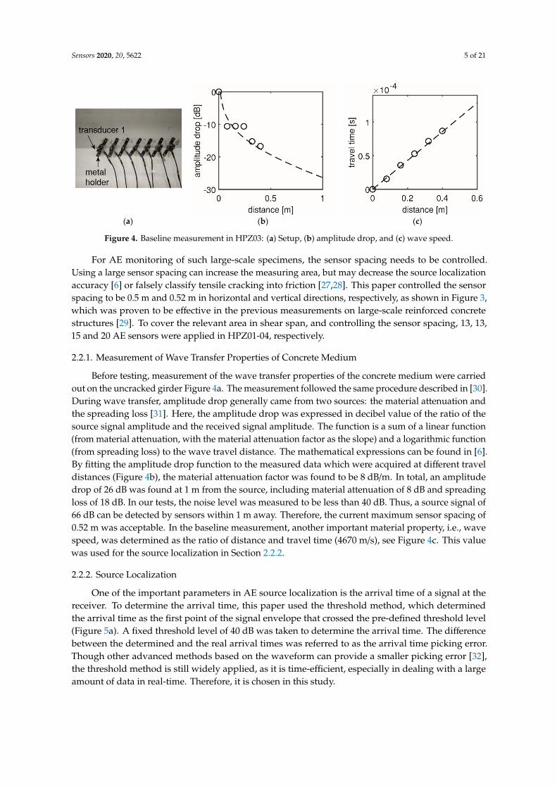
Figure 4. Baseline measurement in HPZ03: (a) Setup, (b) amplitude drop, and (c) wave speed.

For AE monitoring of such large-scale specimens, the sensor spacing needs to be controlled. Using a large sensor spacing can increase the measuring area, but may decrease the source localization accuracy [6] or falsely classify tensile cracking into friction [27,28]. This paper controlled the sensor spacing to be 0.5 m and 0.52 m in horizontal and vertical directions, respectively, as shown in Figure 3, which was proven to be effective in the previous measurements on large-scale reinforced concrete structures [29]. To cover the relevant area in shear span, and controlling the sensor spacing, 13, 13, 15 and 20 AE sensors were applied in HPZ01-04, respectively.

2.2.1. Measurement of Wave Transfer Properties of Concrete Medium

Before testing, measurement of the wave transfer properties of the concrete medium were carried out on the uncracked girder Figure 4a. The measurement followed the same procedure described in [30]. During wave transfer, amplitude drop generally came from two sources: the material attenuation and the spreading loss [31]. Here, the amplitude drop was expressed in decibel value of the ratio of the source signal amplitude and the received signal amplitude. The function is a sum of a linear function (from material attenuation, with the material attenuation factor as the slope) and a logarithmic function (from spreading loss) to the wave travel distance. The mathematical expressions can be found in [6]. By fitting the amplitude drop function to the measured data which were acquired at different travel distances (Figure 4b), the material attenuation factor was found to be 8 dB/m. In total, an amplitude drop of 26 dB was found at 1 m from the source, including material attenuation of 8 dB and spreading loss of 18 dB. In our tests, the noise level was measured to be less than 40 dB. Thus, a source signal of 66 dB can be detected by sensors within 1 m away. Therefore, the current maximum sensor spacing of 0.52 m was acceptable. In the baseline measurement, another important material property, i.e., wave speed, was determined as the ratio of distance and travel time (4670 m/s), see Figure 4c. This value was used for the source localization in Section 2.2.2.

2.2.2. Source Localization

One of the important parameters in AE source localization is the arrival time of a signal at the receiver. To determine the arrival time, this paper used the threshold method, which determined the arrival time as the first point of the signal envelope that crossed the pre-defined threshold level (Figure 5a). A fixed threshold level of 40 dB was taken to determine the arrival time. The difference between the determined and the real arrival times was referred to as the arrival time picking error. Though other advanced methods based on the waveform can provide a smaller picking error [32], the threshold method is still widely applied, as it is time-efficient, especially in dealing with a large amount of data in real-time. Therefore, it is chosen in this study.

Figure 4. Baseline measurement in HPZ03: (a) Setup, (b) amplitude drop, and (c) wave speed.

For AE monitoring of such large-scale specimens, the sensor spacing needs to be controlled.Using a large sensor spacing can increase the measuring area, but may decrease the source localizationaccuracy [6] or falsely classify tensile cracking into friction [27,28]. This paper controlled the sensorspacing to be 0.5 m and 0.52 m in horizontal and vertical directions, respectively, as shown in Figure 3,which was proven to be effective in the previous measurements on large-scale reinforced concretestructures [29]. To cover the relevant area in shear span, and controlling the sensor spacing, 13, 13,15 and 20 AE sensors were applied in HPZ01-04, respectively.

2.2.1. Measurement of Wave Transfer Properties of Concrete Medium

Before testing, measurement of the wave transfer properties of the concrete medium were carriedout on the uncracked girder Figure 4a. The measurement followed the same procedure described in [30].During wave transfer, amplitude drop generally came from two sources: the material attenuation andthe spreading loss [31]. Here, the amplitude drop was expressed in decibel value of the ratio of thesource signal amplitude and the received signal amplitude. The function is a sum of a linear function(from material attenuation, with the material attenuation factor as the slope) and a logarithmic function(from spreading loss) to the wave travel distance. The mathematical expressions can be found in [6].By fitting the amplitude drop function to the measured data which were acquired at different traveldistances (Figure 4b), the material attenuation factor was found to be 8 dB/m. In total, an amplitudedrop of 26 dB was found at 1 m from the source, including material attenuation of 8 dB and spreadingloss of 18 dB. In our tests, the noise level was measured to be less than 40 dB. Thus, a source signal of66 dB can be detected by sensors within 1 m away. Therefore, the current maximum sensor spacing of0.52 m was acceptable. In the baseline measurement, another important material property, i.e., wavespeed, was determined as the ratio of distance and travel time (4670 m/s), see Figure 4c. This valuewas used for the source localization in Section 2.2.2.

2.2.2. Source Localization

One of the important parameters in AE source localization is the arrival time of a signal at thereceiver. To determine the arrival time, this paper used the threshold method, which determinedthe arrival time as the first point of the signal envelope that crossed the pre-defined threshold level(Figure 5a). A fixed threshold level of 40 dB was taken to determine the arrival time. The differencebetween the determined and the real arrival times was referred to as the arrival time picking error.Though other advanced methods based on the waveform can provide a smaller picking error [32],the threshold method is still widely applied, as it is time-efficient, especially in dealing with a largeamount of data in real-time. Therefore, it is chosen in this study.

Sensors 2020, 20, 5622 6 of 21


(a) (b)

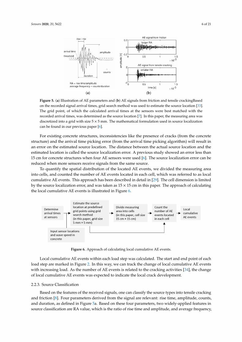
Figure 5. (a) Illustration of AE parameters and (b) AE signals from friction and tensile crackingBased on the recorded signal arrival times, grid search method was used to estimate the source location [33]. The grid point, of which the calculated arrival times at the sensors were best matched with the recorded arrival times, was determined as the source location [7]. In this paper, the measuring area was discretized into a grid with size 5 × 5 mm. The mathematical formulation used in source localization can be found in our previous paper [6].

For existing concrete structures, inconsistencies like the presence of cracks (from the concrete structure) and the arrival time picking error (from the arrival time picking algorithm) will result in an error on the estimated source location. The distance between the actual source location and the estimated location is called the source localization error. A previous study showed an error less than 15 cm for concrete structures when four AE sensors were used [6]. The source localization error can be reduced when more sensors receive signals from the same source.

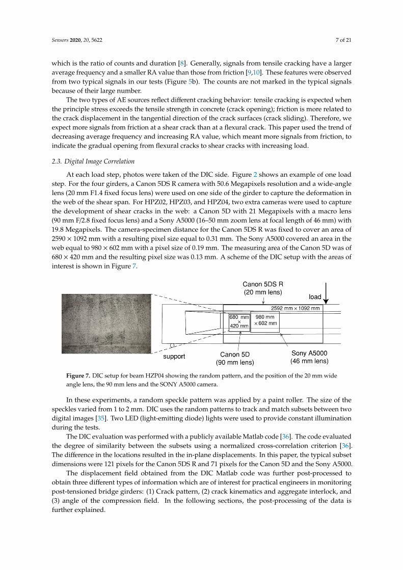
To quantify the spatial distribution of the located AE events, we divided the measuring area into cells, and counted the number of AE events located in each cell, which was referred to as local cumulative AE events. This approach has been described in detail in [29]. The cell dimension is limited by the source localization error, and was taken as 15 × 15 cm in this paper. The approach of calculating the local cumulative AE events is illustrated in Figure 6.

Figure 6. Approach of calculating local cumulative AE events.

Local cumulative AE events within each load step was calculated. The start and end point of each load step are marked in Figure 2. In this way, we can track the change of local cumulative AE events with increasing load. As the number of AE events is related to the cracking activities [34], the change of local cumulative AE events was expected to indicate the local crack development.

2.2.3. Source Classification

Based on the features of the received signals, one can classify the source types into tensile cracking and friction [8]. Four parameters derived from the signal are relevant: rise time, amplitude, counts, and duration, as defined in Figure 5a. Based on these four parameters, two widely-applied features in source classification are RA value, which is the ratio of rise time and amplitude, and average frequency, which is the ratio of counts and duration [8]. Generally, signals from tensile cracking have a larger average frequency and a smaller RA value than those from friction [9,10].

Figure 5. (a) Illustration of AE parameters and (b) AE signals from friction and tensile crackingBasedon the recorded signal arrival times, grid search method was used to estimate the source location [33].The grid point, of which the calculated arrival times at the sensors were best matched with therecorded arrival times, was determined as the source location [7]. In this paper, the measuring area wasdiscretized into a grid with size 5 × 5 mm. The mathematical formulation used in source localizationcan be found in our previous paper [6].

For existing concrete structures, inconsistencies like the presence of cracks (from the concretestructure) and the arrival time picking error (from the arrival time picking algorithm) will result inan error on the estimated source location. The distance between the actual source location and theestimated location is called the source localization error. A previous study showed an error less than15 cm for concrete structures when four AE sensors were used [6]. The source localization error can bereduced when more sensors receive signals from the same source.

To quantify the spatial distribution of the located AE events, we divided the measuring areainto cells, and counted the number of AE events located in each cell, which was referred to as localcumulative AE events. This approach has been described in detail in [29]. The cell dimension is limitedby the source localization error, and was taken as 15 × 15 cm in this paper. The approach of calculatingthe local cumulative AE events is illustrated in Figure 6.


(a) (b)

Figure 5. (a) Illustration of AE parameters and (b) AE signals from friction and tensile crackingBased on the recorded signal arrival times, grid search method was used to estimate the source location [33]. The grid point, of which the calculated arrival times at the sensors were best matched with the recorded arrival times, was determined as the source location [7]. In this paper, the measuring area was discretized into a grid with size 5 × 5 mm. The mathematical formulation used in source localization can be found in our previous paper [6].

For existing concrete structures, inconsistencies like the presence of cracks (from the concrete structure) and the arrival time picking error (from the arrival time picking algorithm) will result in an error on the estimated source location. The distance between the actual source location and the estimated location is called the source localization error. A previous study showed an error less than 15 cm for concrete structures when four AE sensors were used [6]. The source localization error can be reduced when more sensors receive signals from the same source.

To quantify the spatial distribution of the located AE events, we divided the measuring area into cells, and counted the number of AE events located in each cell, which was referred to as local cumulative AE events. This approach has been described in detail in [29]. The cell dimension is limited by the source localization error, and was taken as 15 × 15 cm in this paper. The approach of calculating the local cumulative AE events is illustrated in Figure 6.


Local cumulative AE events within each load step was calculated. The start and end point of each load step are marked in Figure 2. In this way, we can track the change of local cumulative AE events with increasing load. As the number of AE events is related to the cracking activities [34], the change of local cumulative AE events was expected to indicate the local crack development.


Based on the features of the received signals, one can classify the source types into tensile cracking and friction [8]. Four parameters derived from the signal are relevant: rise time, amplitude, counts, and duration, as defined in Figure 5a. Based on these four parameters, two widely-applied features in source classification are RA value, which is the ratio of rise time and amplitude, and average frequency, which is the ratio of counts and duration [8]. Generally, signals from tensile cracking have a larger average frequency and a smaller RA value than those from friction [9,10].


Local cumulative AE events within each load step was calculated. The start and end point of eachload step are marked in Figure 2. In this way, we can track the change of local cumulative AE eventswith increasing load. As the number of AE events is related to the cracking activities [34], the changeof local cumulative AE events was expected to indicate the local crack development.


Based on the features of the received signals, one can classify the source types into tensile crackingand friction [8]. Four parameters derived from the signal are relevant: rise time, amplitude, counts,and duration, as defined in Figure 5a. Based on these four parameters, two widely-applied features insource classification are RA value, which is the ratio of rise time and amplitude, and average frequency,

Sensors 2020, 20, 5622 7 of 21

which is the ratio of counts and duration [8]. Generally, signals from tensile cracking have a largeraverage frequency and a smaller RA value than those from friction [9,10]. These features were observedfrom two typical signals in our tests (Figure 5b). The counts are not marked in the typical signalsbecause of their large number.

The two types of AE sources reflect different cracking behavior: tensile cracking is expected whenthe principle stress exceeds the tensile strength in concrete (crack opening); friction is more related tothe crack displacement in the tangential direction of the crack surfaces (crack sliding). Therefore, weexpect more signals from friction at a shear crack than at a flexural crack. This paper used the trend ofdecreasing average frequency and increasing RA value, which meant more signals from friction, toindicate the gradual opening from flexural cracks to shear cracks with increasing load.

2.3. Digital Image Correlation

At each load step, photos were taken of the DIC side. Figure 2 shows an example of one loadstep. For the four girders, a Canon 5DS R camera with 50.6 Megapixels resolution and a wide-anglelens (20 mm F1.4 fixed focus lens) were used on one side of the girder to capture the deformation inthe web of the shear span. For HPZ02, HPZ03, and HPZ04, two extra cameras were used to capturethe development of shear cracks in the web: a Canon 5D with 21 Megapixels with a macro lens(90 mm F/2.8 fixed focus lens) and a Sony A5000 (16–50 mm zoom lens at focal length of 46 mm) with19.8 Megapixels. The camera-specimen distance for the Canon 5DS R was fixed to cover an area of2590 × 1092 mm with a resulting pixel size equal to 0.31 mm. The Sony A5000 covered an area in theweb equal to 980 × 602 mm with a pixel size of 0.19 mm. The measuring area of the Canon 5D was of680 × 420 mm and the resulting pixel size was 0.13 mm. A scheme of the DIC setup with the areas ofinterest is shown in Figure 7.


These features were observed from two typical signals in our tests (Figure 5b). The counts are not marked in the typical signals because of their large number.

The two types of AE sources reflect different cracking behavior: tensile cracking is expected when the principle stress exceeds the tensile strength in concrete (crack opening); friction is more related to the crack displacement in the tangential direction of the crack surfaces (crack sliding). Therefore, we expect more signals from friction at a shear crack than at a flexural crack. This paper used the trend of decreasing average frequency and increasing RA value, which meant more signals from friction, to indicate the gradual opening from flexural cracks to shear cracks with increasing load.

2.3. Digital Image Correlation

At each load step, photos were taken of the DIC side. Figure 2 shows an example of one load step. For the four girders, a Canon 5DS R camera with 50.6 Megapixels resolution and a wide-angle lens (20 mm F1.4 fixed focus lens) were used on one side of the girder to capture the deformation in the web of the shear span. For HPZ02, HPZ03, and HPZ04, two extra cameras were used to capture the development of shear cracks in the web: a Canon 5D with 21 Megapixels with a macro lens (90 mm F/2.8 fixed focus lens) and a Sony A5000 (16–50 mm zoom lens at focal length of 46 mm) with 19.8 Megapixels. The camera-specimen distance for the Canon 5DS R was fixed to cover an area of 2590 × 1092 mm with a resulting pixel size equal to 0.31 mm. The Sony A5000 covered an area in the web equal to 980 × 602 mm with a pixel size of 0.19 mm. The measuring area of the Canon 5D was of 680 × 420 mm and the resulting pixel size was 0.13 mm. A scheme of the DIC setup with the areas of interest is shown in Figure 7.

Figure 7. DIC setup for beam HZP04 showing the random pattern, and the position of the 20 mm wide angle lens, the 90 mm lens and the SONY A5000 camera.

In these experiments, a random speckle pattern was applied by a paint roller. The size of the speckles varied from 1 to 2 mm. DIC uses the random patterns to track and match subsets between two digital images [35]. Two LED (light-emitting diode) lights were used to provide constant illumination during the tests.

The DIC evaluation was performed with a publicly available Matlab code [36]. The code evaluated the degree of similarity between the subsets using a normalized cross-correlation criterion [36]. The difference in the locations resulted in the in-plane displacements. In this paper, the typical subset dimensions were 121 pixels for the Canon 5DS R and 71 pixels for the Canon 5D and the Sony A5000.

The displacement field obtained from the DIC Matlab code was further post-processed to obtain three different types of information which are of interest for practical engineers in monitoring post-tensioned bridge girders: (1) Crack pattern, (2) crack kinematics and aggregate interlock, and (3) angle of the compression field. In the following sections, the post-processing of the data is further explained.

Figure 7. DIC setup for beam HZP04 showing the random pattern, and the position of the 20 mm wideangle lens, the 90 mm lens and the SONY A5000 camera.

In these experiments, a random speckle pattern was applied by a paint roller. The size of thespeckles varied from 1 to 2 mm. DIC uses the random patterns to track and match subsets between twodigital images [35]. Two LED (light-emitting diode) lights were used to provide constant illuminationduring the tests.

The DIC evaluation was performed with a publicly available Matlab code [36]. The code evaluatedthe degree of similarity between the subsets using a normalized cross-correlation criterion [36].The difference in the locations resulted in the in-plane displacements. In this paper, the typical subsetdimensions were 121 pixels for the Canon 5DS R and 71 pixels for the Canon 5D and the Sony A5000.

The displacement field obtained from the DIC Matlab code was further post-processed toobtain three different types of information which are of interest for practical engineers in monitoringpost-tensioned bridge girders: (1) Crack pattern, (2) crack kinematics and aggregate interlock, and(3) angle of the compression field. In the following sections, the post-processing of the data isfurther explained.

Sensors 2020, 20, 5622 8 of 21

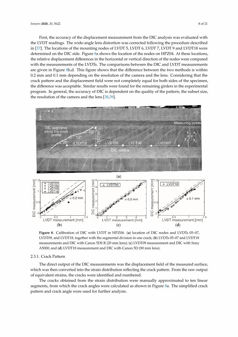
First, the accuracy of the displacement measurement from the DIC analysis was evaluated withthe LVDT readings. The wide-angle lens distortion was corrected following the procedure describedin [37]. The locations of the mounting nodes of LVDT 5, LVDT 6, LVDT 7, LVDT 9 and LVDT18 weredetermined on the DIC side. Figure 8a shows the location of the nodes on HPZ04. At these locations,the relative displacement differences in the horizontal or vertical direction of the nodes were comparedwith the measurements of the LVDTs. The comparisons between the DIC and LVDT measurementsare given in Figure 8b,d. This figure shows that the difference between the two methods is within0.2 mm and 0.1 mm depending on the resolution of the camera and the lens. Considering that thecrack pattern and the displacement field were not completely equal for both sides of the specimen,the difference was acceptable. Similar results were found for the remaining girders in the experimentalprogram. In general, the accuracy of DIC is dependent on the quality of the pattern, the subset size,the resolution of the camera and the lens [38,39].


First, the accuracy of the displacement measurement from the DIC analysis was evaluated with the LVDT readings. The wide-angle lens distortion was corrected following the procedure described in [37]. The locations of the mounting nodes of LVDT 5, LVDT 6, LVDT 7, LVDT 9 and LVDT18 were determined on the DIC side. Figure 8a shows the location of the nodes on HPZ04. At these locations, the relative displacement differences in the horizontal or vertical direction of the nodes were compared with the measurements of the LVDTs. The comparisons between the DIC and LVDT measurements are given in Figure 8b,d. This figure shows that the difference between the two methods is within 0.2 mm and 0.1 mm depending on the resolution of the camera and the lens. Considering that the crack pattern and the displacement field were not completely equal for both sides of the specimen, the difference was acceptable. Similar results were found for the remaining girders in the experimental program. In general, the accuracy of DIC is dependent on the quality of the pattern, the subset size, the resolution of the camera and the lens [38,39].

(a)

(b) (c) (d)

Figure 8. Calibration of DIC with LVDT in HPZ04: (a) location of DIC nodes and LVDTs 05–07, LVDT09, and LVDT18, together with the segmental division in one crack; (b) LVDTs 05–07 and LVDT18 measurements and DIC with Canon 5DS R (20 mm lens); (c) LVDT09 measurement and DIC with Sony A5000; and (d) LVDT18 measurement and DIC with Canon 5D (90 mm lens).

2.3.1. Crack Pattern

The direct output of the DIC measurements was the displacement field of the measured surface, which was then converted into the strain distribution reflecting the crack pattern. From the raw output of equivalent strains, the cracks were identified and numbered.

The cracks obtained from the strain distribution were manually approximated to ten linear segments, from which the crack angles were calculated as shown in Figure 8a. The simplified crack pattern and crack angle were used for further analysis.

2.3.2. Crack Kinematics and Aggregate Interlock

Figure 8. Calibration of DIC with LVDT in HPZ04: (a) location of DIC nodes and LVDTs 05–07,LVDT09, and LVDT18, together with the segmental division in one crack; (b) LVDTs 05–07 and LVDT18measurements and DIC with Canon 5DS R (20 mm lens); (c) LVDT09 measurement and DIC with SonyA5000; and (d) LVDT18 measurement and DIC with Canon 5D (90 mm lens).

2.3.1. Crack Pattern

The direct output of the DIC measurements was the displacement field of the measured surface,which was then converted into the strain distribution reflecting the crack pattern. From the raw outputof equivalent strains, the cracks were identified and numbered.

The cracks obtained from the strain distribution were manually approximated to ten linearsegments, from which the crack angles were calculated as shown in Figure 8a. The simplified crackpattern and crack angle were used for further analysis.

Sensors 2020, 20, 5622 9 of 21

2.3.2. Crack Kinematics and Aggregate Interlock

The DIC measurements allowed the determination of the crack kinematics in a detailed manner.The results of crack kinematics were divided into the displacement difference along the x and ydirection, and the displacements along the crack profile.

For each crack, two measuring points on both sides of the crack profile were determined.The displacement difference in the x-direction was defined as W (crack opening in the longitudinaldirection), and the displacement difference in the y-direction was defined as ∆ (crack opening in thetransverse direction). An example of the measuring points is given in Figure 8a as xi and yi.

The crack kinematics in the global coordinate system were further converted to a local coordinatesystem along the simplified crack profile using the angle of the ten segments. As such, the local normaland tangential displacements were obtained. Detailed information about the algorithm can be foundin [37].

The aggregate interlock stresses were computed using the normal and tangential displacementsobtained directly from the DIC measurements as an input to Walraven’s formulation for aggregateinterlock [40]. In Walraven’s model, the aggregates are simplified to rigid spheres and the cementmatrix is an ideal plastic material. Slipping of the interface and crushing of the cement paste at thecontact area generate the shear and normal stresses. The resulting forces are obtained by integratingthe stresses along the crack profile. The normal and shear stresses are given as:(

στ

)= σpu

(Ay + µAx

Ax − µAy

)(1)

where σpu is the compressive strength of the cement matrix, µ is the coefficient of friction, Ax, Ay are theprojected contact areas between the surfaces of the aggregates and the cement matrix. The projectedcontact areas (Ax and Ay) depend on the magnitude of the normal (n) and tangential (t) displacementsof the crack faces. Other influencing factors are the relative volume of aggregates and the distributionof the aggregate diameter.

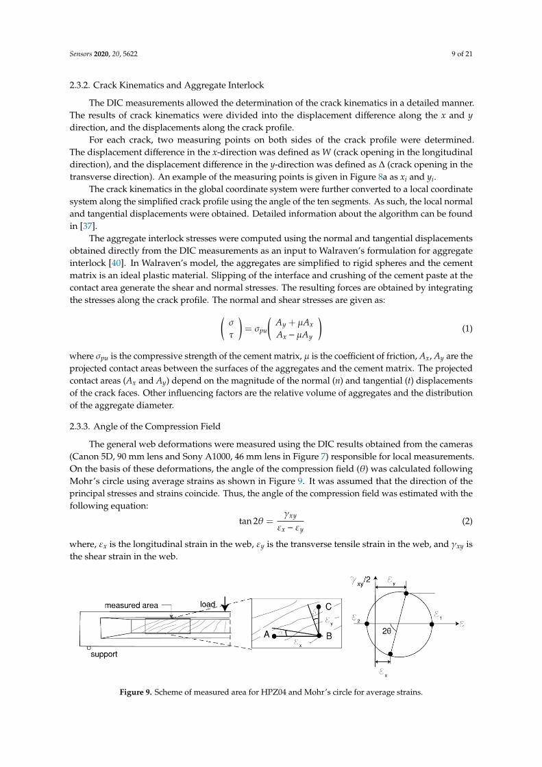
2.3.3. Angle of the Compression Field

The general web deformations were measured using the DIC results obtained from the cameras(Canon 5D, 90 mm lens and Sony A1000, 46 mm lens in Figure 7) responsible for local measurements.On the basis of these deformations, the angle of the compression field (θ) was calculated followingMohr’s circle using average strains as shown in Figure 9. It was assumed that the direction of theprincipal stresses and strains coincide. Thus, the angle of the compression field was estimated with thefollowing equation:

tan 2θ =γxy

εx − εy(2)

where, εx is the longitudinal strain in the web, εy is the transverse tensile strain in the web, and γxy isthe shear strain in the web.


The DIC measurements allowed the determination of the crack kinematics in a detailed manner. The results of crack kinematics were divided into the displacement difference along the x and y direction, and the displacements along the crack profile.

For each crack, two measuring points on both sides of the crack profile were determined. The displacement difference in the x-direction was defined as W (crack opening in the longitudinal direction), and the displacement difference in the y-direction was defined as ∆ (crack opening in the transverse direction). An example of the measuring points is given in Figure 8a as xi and yi.

The crack kinematics in the global coordinate system were further converted to a local coordinate system along the simplified crack profile using the angle of the ten segments. As such, the local normal and tangential displacements were obtained. Detailed information about the algorithm can be found in [37].

The aggregate interlock stresses were computed using the normal and tangential displacements obtained directly from the DIC measurements as an input to Walraven’s formulation for aggregate interlock [40]. In Walraven’s model, the aggregates are simplified to rigid spheres and the cement matrix is an ideal plastic material. Slipping of the interface and crushing of the cement paste at the contact area generate the shear and normal stresses. The resulting forces are obtained by integrating the stresses along the crack profile. The normal and shear stresses are given as: 𝜎𝜏 = 𝜎 𝐴 + 𝜇𝐴𝐴 − 𝜇𝐴 (1)

where σpu is the compressive strength of the cement matrix, μ is the coefficient of friction, Ax, Ay are the projected contact areas between the surfaces of the aggregates and the cement matrix. The projected contact areas (Ax and Ay) depend on the magnitude of the normal (n) and tangential (t) displacements of the crack faces. Other influencing factors are the relative volume of aggregates and the distribution of the aggregate diameter.


The general web deformations were measured using the DIC results obtained from the cameras (Canon 5D, 90 mm lens and Sony A1000, 46 mm lens in Figure 7) responsible for local measurements. On the basis of these deformations, the angle of the compression field (θ) was calculated following Mohr’s circle using average strains as shown in Figure 9. It was assumed that the direction of the principal stresses and strains coincide. Thus, the angle of the compression field was estimated with the following equation: tan 2𝜃 = 𝛾𝜀 − 𝜀 (2)

where, εx is the longitudinal strain in the web, εy is the transverse tensile strain in the web, and γxy is the shear strain in the web.

Figure 9. Scheme of measured area for HPZ04 and Mohr’s circle for average strains.

An algorithm was developed to select the area of interest and to calculate the average strains (εx, εy, and γxy) from the displacement measurements of the DIC results. The normal strain in the y-direction (εy) was calculated from the average displacements along the vertical line 𝐵𝐶removing

Figure 9. Scheme of measured area for HPZ04 and Mohr’s circle for average strains.

Sensors 2020, 20, 5622 10 of 21

An algorithm was developed to select the area of interest and to calculate the average strains(εx, εy, and γxy) from the displacement measurements of the DIC results. The normal strain in they-direction (εy) was calculated from the average displacements along the vertical line BC removing theoutliers. For the normal strain in the x-direction (εx), a linear strain distribution was assumed along theheight direction with the strain at the top side of the web being zero. When AB is located at the bottomof the web, the assumed distribution result in εx = εxAB/2 with εxAB as the average strains along thehorizontal line AB located at the bottom of the web. The shear strain (γxy) was computed as the changeof the angle between the lines AB and BC, thus γxy = α+ β, with α and β as shown in Figure 9.

With the measured angle of the compression field, we can estimate the number of stirrups activatedusing the NEN-EN 1992-1-1:2-005 [3], expression for the contribution of the stirrups (VRd,s) as follows:

nstirrup =

Asws z fyw cotθ

Asw fyw=

zs

cotθ (3)

where z is the height of lever arm, s is the stirrup spacing, θ is the angle of the compression field, Asw isthe area of the transverse reinforcement, and fyw is the yield strength of the transverse reinforcement.

3. Results

3.1. Tradional Measurement Results

Determination of the failure mode, based on the observations during tests, is presented in thecompanion paper [4]. A brief summary is: HPZ01 and HPZ02 failed by crushing of the compressionstrut between the load and the support (shear-compression failure); HPZ03 failed by local crushing ofconcrete in the top flange; and HPZ04 failed by crushing of the concrete compression field in the webof the girder.

In all experiments, the cracks gradually developed from sections with a higher sectional momentto sections with a lower sectional moment. Three types of cracks were observed: flexural cracks, whichstarted from the bottom of the girder and developed upwards vertically, flexure-shear cracks, whichwere the inclined cracks developed from the previously defined flexural cracks, and shear–tensioncracks, which were the inclined cracks that started in the web.

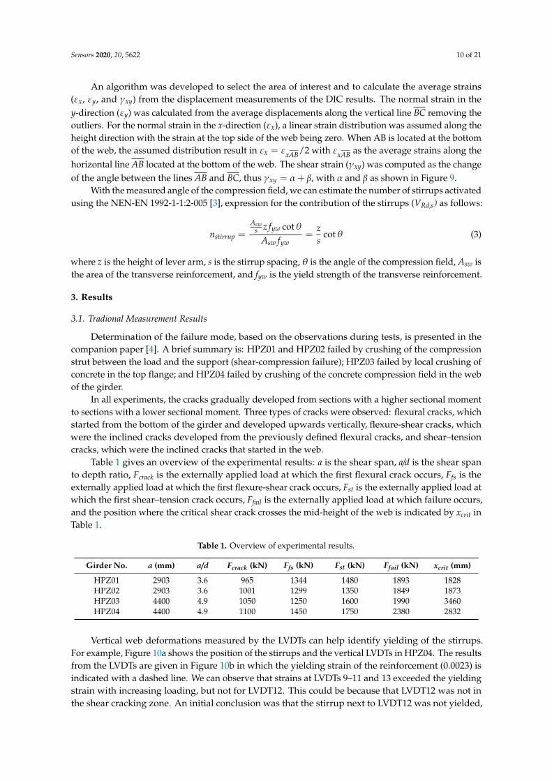
Table 1 gives an overview of the experimental results: a is the shear span, a/d is the shear spanto depth ratio, Fcrack is the externally applied load at which the first flexural crack occurs, Ffs is theexternally applied load at which the first flexure-shear crack occurs, Fst is the externally applied load atwhich the first shear–tension crack occurs, Ffail is the externally applied load at which failure occurs,and the position where the critical shear crack crosses the mid-height of the web is indicated by xcrit inTable 1.

Table 1. Overview of experimental results.

Girder No. a (mm) a/d Fcrack (kN) Ffs (kN) Fst (kN) Ffail (kN) xcrit (mm)

HPZ01 2903 3.6 965 1344 1480 1893 1828HPZ02 2903 3.6 1001 1299 1350 1849 1873HPZ03 4400 4.9 1050 1250 1600 1990 3460HPZ04 4400 4.9 1100 1450 1750 2380 2832

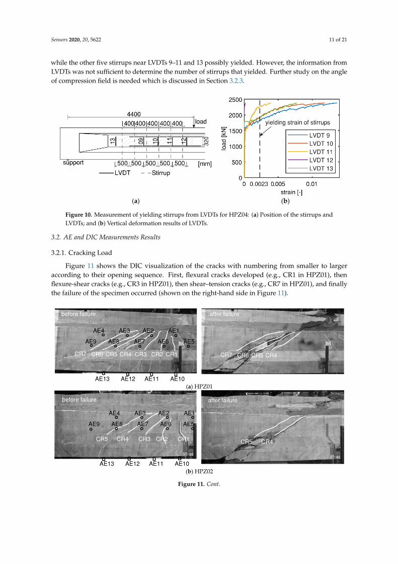
Vertical web deformations measured by the LVDTs can help identify yielding of the stirrups.For example, Figure 10a shows the position of the stirrups and the vertical LVDTs in HPZ04. The resultsfrom the LVDTs are given in Figure 10b in which the yielding strain of the reinforcement (0.0023) isindicated with a dashed line. We can observe that strains at LVDTs 9–11 and 13 exceeded the yieldingstrain with increasing loading, but not for LVDT12. This could be because that LVDT12 was not inthe shear cracking zone. An initial conclusion was that the stirrup next to LVDT12 was not yielded,

Sensors 2020, 20, 5622 11 of 21

while the other five stirrups near LVDTs 9–11 and 13 possibly yielded. However, the information fromLVDTs was not sufficient to determine the number of stirrups that yielded. Further study on the angleof compression field is needed which is discussed in Section 3.2.3.


information from LVDTs was not sufficient to determine the number of stirrups that yielded. Further study on the angle of compression field is needed which is discussed in Section 3.2.3.

(a) (b)

Figure 10. Measurement of yielding stirrups from LVDTs for HPZ04: (a) Position of the stirrups and LVDTs; and (b) Vertical deformation results of LVDTs.

3.2. AE and DIC Measurements Results

3.2.1. Cracking Load

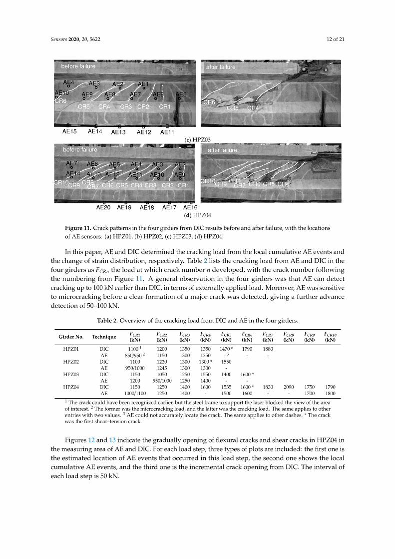
Figure 11 shows the DIC visualization of the cracks with numbering from smaller to larger according to their opening sequence. First, flexural cracks developed (e.g., CR1 in HPZ01), then flexure-shear cracks (e.g., CR3 in HPZ01), then shear–tension cracks (e.g., CR7 in HPZ01), and finally the failure of the specimen occurred (shown on the right-hand side in Figure 11).

(a) HPZ01

(b) HPZ02

Figure 10. Measurement of yielding stirrups from LVDTs for HPZ04: (a) Position of the stirrups andLVDTs; and (b) Vertical deformation results of LVDTs.



Figure 11 shows the DIC visualization of the cracks with numbering from smaller to largeraccording to their opening sequence. First, flexural cracks developed (e.g., CR1 in HPZ01), thenflexure-shear cracks (e.g., CR3 in HPZ01), then shear–tension cracks (e.g., CR7 in HPZ01), and finallythe failure of the specimen occurred (shown on the right-hand side in Figure 11).


information from LVDTs was not sufficient to determine the number of stirrups that yielded. Further study on the angle of compression field is needed which is discussed in Section 3.2.3.

(a) (b)

Figure 10. Measurement of yielding stirrups from LVDTs for HPZ04: (a) Position of the stirrups and LVDTs; and (b) Vertical deformation results of LVDTs.



Figure 11 shows the DIC visualization of the cracks with numbering from smaller to larger according to their opening sequence. First, flexural cracks developed (e.g., CR1 in HPZ01), then flexure-shear cracks (e.g., CR3 in HPZ01), then shear–tension cracks (e.g., CR7 in HPZ01), and finally the failure of the specimen occurred (shown on the right-hand side in Figure 11).

(a) HPZ01

(b) HPZ02

Figure 11. Cont.

Sensors 2020, 20, 5622 12 of 21


(c) HPZ03

(d) HPZ04

Figure 11. Crack patterns in the four girders from DIC results before and after failure, with the locations of AE sensors: (a) HPZ01, (b) HPZ02, (c) HPZ03, (d) HPZ04.

In this paper, AE and DIC determined the cracking load from the local cumulative AE events and the change of strain distribution, respectively. Table 2 lists the cracking load from AE and DIC in the four girders as FCRn the load at which crack number n developed, with the crack number following the numbering from Figure 11. A general observation in the four girders was that AE can detect cracking up to 100 kN earlier than DIC, in terms of externally applied load. Moreover, AE was sensitive to microcracking before a clear formation of a major crack was detected, giving a further advance detection of 50–100 kN.

Table 2. Overview of the cracking load from DIC and AE in the four girders.

Girder No.

Technique FCR1 (kN) FCR2 (kN) FCR3 (kN)

FCR4 (kN)

FCR5 (kN)

FCR6 (kN)

FCR7 (kN)

FCR8 (kN)

FCR9 (kN)

FCR10 (kN)

HPZ01 DIC 1100 1 1200 1350 1350 1470

* 1790 1880

AE 850/950 2 1150 1300 1350 - 3 - -

HPZ02 DIC 1100 1220 1300 1300 *

1550

AE 950/1000 1245 1300 1300 -

HPZ03 DIC 1150 1050 1250 1550 1400 1600

*

AE 1200 950/1000 1250 1400 - -

HPZ04 DIC 1150 1250 1400 1600 1535 1600

* 1830 2090 1750 1790

AE 1000/1100 1250 1400 - 1500 1600 - - 1700 1800 1 The crack could have been recognized earlier, but the steel frame to support the laser blocked the view of the area of interest. 2 The former was the microcracking load, and the latter was the cracking load. The same applies to other entries with two values. 3 AE could not accurately locate the crack. The same applies to other dashes. * The crack was the first shear–tension crack.

Figures 12 and 13 indicate the gradually opening of flexural cracks and shear cracks in HPZ04 in the measuring area of AE and DIC. For each load step, three types of plots are included: the first one is the estimated location of AE events that occurred in this load step, the second one shows the local cumulative AE events, and the third one is the incremental crack opening from DIC. The interval of each load step is 50 kN.

Figure 11. Crack patterns in the four girders from DIC results before and after failure, with the locationsof AE sensors: (a) HPZ01, (b) HPZ02, (c) HPZ03, (d) HPZ04.

In this paper, AE and DIC determined the cracking load from the local cumulative AE events andthe change of strain distribution, respectively. Table 2 lists the cracking load from AE and DIC in thefour girders as FCRn the load at which crack number n developed, with the crack number followingthe numbering from Figure 11. A general observation in the four girders was that AE can detectcracking up to 100 kN earlier than DIC, in terms of externally applied load. Moreover, AE was sensitiveto microcracking before a clear formation of a major crack was detected, giving a further advancedetection of 50–100 kN.

Table 2. Overview of the cracking load from DIC and AE in the four girders.

Girder No. Technique FCR1(kN)

FCR2(kN)

FCR3(kN)

FCR4(kN)

FCR5(kN)

FCR6(kN)

FCR7(kN)

FCR8(kN)

FCR9(kN)

FCR10(kN)

HPZ01 DIC 1100 1 1200 1350 1350 1470 * 1790 1880AE 850/950 2 1150 1300 1350 - 3 - -

HPZ02 DIC 1100 1220 1300 1300 * 1550AE 950/1000 1245 1300 1300 -

HPZ03 DIC 1150 1050 1250 1550 1400 1600 *AE 1200 950/1000 1250 1400 - -

HPZ04 DIC 1150 1250 1400 1600 1535 1600 * 1830 2090 1750 1790AE 1000/1100 1250 1400 - 1500 1600 - - 1700 1800

1 The crack could have been recognized earlier, but the steel frame to support the laser blocked the view of the areaof interest. 2 The former was the microcracking load, and the latter was the cracking load. The same applies to otherentries with two values. 3 AE could not accurately locate the crack. The same applies to other dashes. * The crackwas the first shear–tension crack.

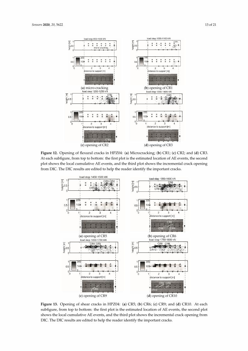
Figures 12 and 13 indicate the gradually opening of flexural cracks and shear cracks in HPZ04 inthe measuring area of AE and DIC. For each load step, three types of plots are included: the first one isthe estimated location of AE events that occurred in this load step, the second one shows the localcumulative AE events, and the third one is the incremental crack opening from DIC. The interval ofeach load step is 50 kN.

Sensors 2020, 20, 5622 13 of 21


(a) micro-cracking (b) opening of CR1

(c) opening of CR2 (d) opening of CR3

Figure 12. Opening of flexural cracks in HPZ04: (a) Microcracking; (b) CR1; (c) CR2; and (d) CR3. At each subfigure, from top to bottom: the first plot is the estimated location of AE events, the second plot shows the local cumulative AE events, and the third plot shows the incremental crack opening from DIC. The DIC results are edited to help the reader identify the important cracks.

(a) opening of CR5 (b) opening of CR6


Figure 12. Opening of flexural cracks in HPZ04: (a) Microcracking; (b) CR1; (c) CR2; and (d) CR3.At each subfigure, from top to bottom: the first plot is the estimated location of AE events, the secondplot shows the local cumulative AE events, and the third plot shows the incremental crack openingfrom DIC. The DIC results are edited to help the reader identify the important cracks.


(a) micro-cracking (b) opening of CR1


Figure 12. Opening of flexural cracks in HPZ04: (a) Microcracking; (b) CR1; (c) CR2; and (d) CR3. At each subfigure, from top to bottom: the first plot is the estimated location of AE events, the second plot shows the local cumulative AE events, and the third plot shows the incremental crack opening from DIC. The DIC results are edited to help the reader identify the important cracks.

(a) opening of CR5 (b) opening of CR6


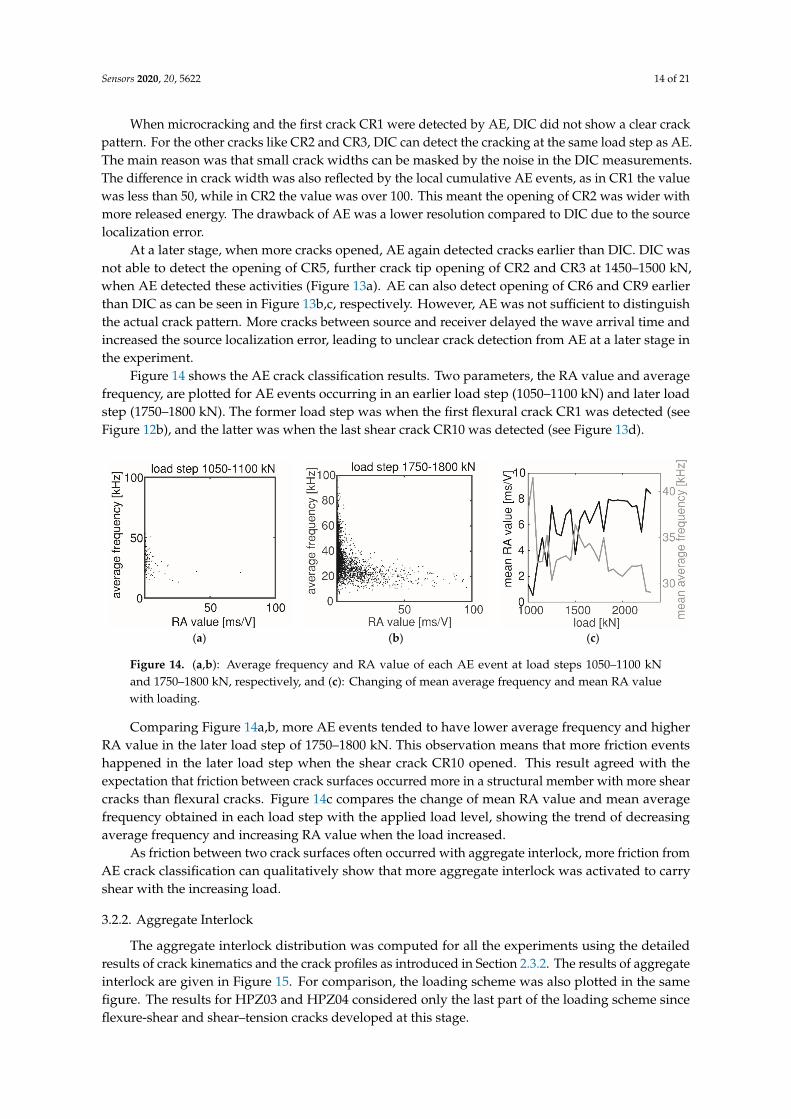
Figure 13. Opening of shear cracks in HPZ04: (a) CR5; (b) CR6; (c) CR9; and (d) CR10. At eachsubfigure, from top to bottom: the first plot is the estimated location of AE events, the second plotshows the local cumulative AE events, and the third plot shows the incremental crack opening fromDIC. The DIC results are edited to help the reader identify the important cracks.

Sensors 2020, 20, 5622 14 of 21

When microcracking and the first crack CR1 were detected by AE, DIC did not show a clear crackpattern. For the other cracks like CR2 and CR3, DIC can detect the cracking at the same load step as AE.The main reason was that small crack widths can be masked by the noise in the DIC measurements.The difference in crack width was also reflected by the local cumulative AE events, as in CR1 the valuewas less than 50, while in CR2 the value was over 100. This meant the opening of CR2 was wider withmore released energy. The drawback of AE was a lower resolution compared to DIC due to the sourcelocalization error.

At a later stage, when more cracks opened, AE again detected cracks earlier than DIC. DIC wasnot able to detect the opening of CR5, further crack tip opening of CR2 and CR3 at 1450–1500 kN,when AE detected these activities (Figure 13a). AE can also detect opening of CR6 and CR9 earlierthan DIC as can be seen in Figure 13b,c, respectively. However, AE was not sufficient to distinguishthe actual crack pattern. More cracks between source and receiver delayed the wave arrival time andincreased the source localization error, leading to unclear crack detection from AE at a later stage inthe experiment.

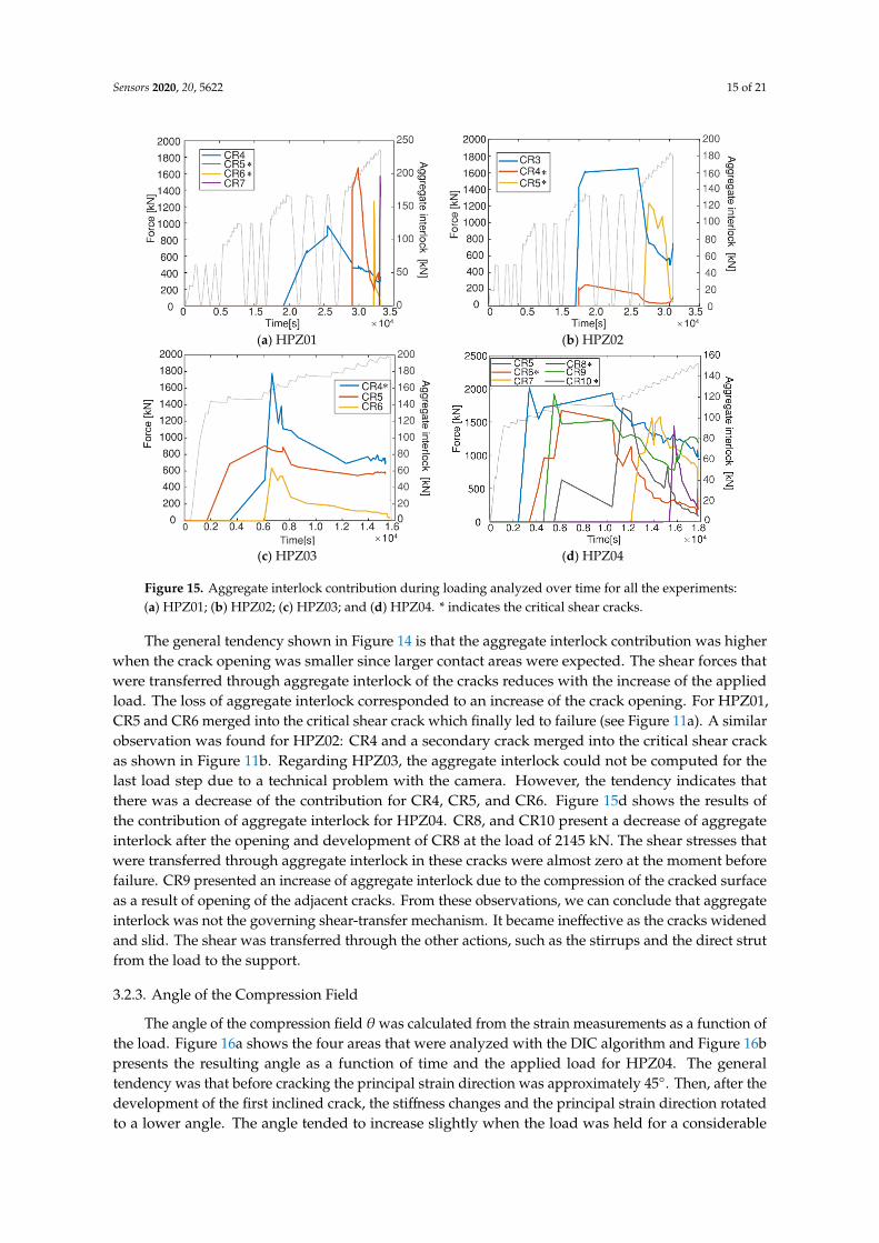
Figure 14 shows the AE crack classification results. Two parameters, the RA value and averagefrequency, are plotted for AE events occurring in an earlier load step (1050–1100 kN) and later loadstep (1750–1800 kN). The former load step was when the first flexural crack CR1 was detected (seeFigure 12b), and the latter was when the last shear crack CR10 was detected (see Figure 13d).


Figure 13. Opening of shear cracks in HPZ04: (a) CR5; (b) CR6; (c) CR9; and (d) CR10. At each subfigure, from top to bottom: the first plot is the estimated location of AE events, the second plot shows the local cumulative AE events, and the third plot shows the incremental crack opening from DIC. The DIC results are edited to help the reader identify the important cracks.

When microcracking and the first crack CR1 were detected by AE, DIC did not show a clear crack pattern. For the other cracks like CR2 and CR3, DIC can detect the cracking at the same load step as AE. The main reason was that small crack widths can be masked by the noise in the DIC measurements. The difference in crack width was also reflected by the local cumulative AE events, as in CR1 the value was less than 50, while in CR2 the value was over 100. This meant the opening of CR2 was wider with more released energy. The drawback of AE was a lower resolution compared to DIC due to the source localization error.

At a later stage, when more cracks opened, AE again detected cracks earlier than DIC. DIC was not able to detect the opening of CR5, further crack tip opening of CR2 and CR3 at 1450–1500 kN, when AE detected these activities (Figure 13a). AE can also detect opening of CR6 and CR9 earlier than DIC as can be seen in Figure 13b,c, respectively. However, AE was not sufficient to distinguish the actual crack pattern. More cracks between source and receiver delayed the wave arrival time and increased the source localization error, leading to unclear crack detection from AE at a later stage in the experiment.

Figure 14 shows the AE crack classification results. Two parameters, the RA value and average frequency, are plotted for AE events occurring in an earlier load step (1050–1100 kN) and later load step (1750–1800 kN). The former load step was when the first flexural crack CR1 was detected (see Figure 12b), and the latter was when the last shear crack CR10 was detected (see Figure 13d).

(a) (b) (c)

Figure 14. (a,b): Average frequency and RA value of each AE event at load steps 1050–1100 kN and 1750–1800 kN, respectively, and (c): Changing of mean average frequency and mean RA value with loading.

Comparing Figure 14a,b, more AE events tended to have lower average frequency and higher RA value in the later load step of 1750–1800 kN. This observation means that more friction events happened in the later load step when the shear crack CR10 opened. This result agreed with the expectation that friction between crack surfaces occurred more in a structural member with more shear cracks than flexural cracks. Figure 14c compares the change of mean RA value and mean average frequency obtained in each load step with the applied load level, showing the trend of decreasing average frequency and increasing RA value when the load increased.

As friction between two crack surfaces often occurred with aggregate interlock, more friction from AE crack classification can qualitatively show that more aggregate interlock was activated to carry shear with the increasing load.

3.2.2. Aggregate Interlock

The aggregate interlock distribution was computed for all the experiments using the detailed results of crack kinematics and the crack profiles as introduced in Section 2.3.2. The results of

Figure 14. (a,b): Average frequency and RA value of each AE event at load steps 1050–1100 kNand 1750–1800 kN, respectively, and (c): Changing of mean average frequency and mean RA valuewith loading.

Comparing Figure 14a,b, more AE events tended to have lower average frequency and higherRA value in the later load step of 1750–1800 kN. This observation means that more friction eventshappened in the later load step when the shear crack CR10 opened. This result agreed with theexpectation that friction between crack surfaces occurred more in a structural member with more shearcracks than flexural cracks. Figure 14c compares the change of mean RA value and mean averagefrequency obtained in each load step with the applied load level, showing the trend of decreasingaverage frequency and increasing RA value when the load increased.

As friction between two crack surfaces often occurred with aggregate interlock, more friction fromAE crack classification can qualitatively show that more aggregate interlock was activated to carryshear with the increasing load.

3.2.2. Aggregate Interlock

The aggregate interlock distribution was computed for all the experiments using the detailedresults of crack kinematics and the crack profiles as introduced in Section 2.3.2. The results of aggregateinterlock are given in Figure 15. For comparison, the loading scheme was also plotted in the samefigure. The results for HPZ03 and HPZ04 considered only the last part of the loading scheme sinceflexure-shear and shear–tension cracks developed at this stage.

Sensors 2020, 20, 5622 15 of 21


aggregate interlock are given in Figure 15. For comparison, the loading scheme was also plotted in the same figure. The results for HPZ03 and HPZ04 considered only the last part of the loading scheme since flexure-shear and shear–tension cracks developed at this stage.

(a) HPZ01 (b) HPZ02

(c) HPZ03 (d) HPZ04

Figure 15. Aggregate interlock contribution during loading analyzed over time for all the experiments: (a) HPZ01; (b) HPZ02; (c) HPZ03; and (d) HPZ04. * indicates the critical shear cracks.

The general tendency shown in Figure 14 is that the aggregate interlock contribution was higher when the crack opening was smaller since larger contact areas were expected. The shear forces that were transferred through aggregate interlock of the cracks reduces with the increase of the applied load. The loss of aggregate interlock corresponded to an increase of the crack opening. For HPZ01, CR5 and CR6 merged into the critical shear crack which finally led to failure (see Figure 11a). A similar observation was found for HPZ02: CR4 and a secondary crack merged into the critical shear crack as shown in Figure 11b. Regarding HPZ03, the aggregate interlock could not be computed for the last load step due to a technical problem with the camera. However, the tendency indicates that there was a decrease of the contribution for CR4, CR5, and CR6. Figure 15d shows the results of the contribution of aggregate interlock for HPZ04. CR8, and CR10 present a decrease of aggregate interlock after the opening and development of CR8 at the load of 2145 kN. The shear stresses that were transferred through aggregate interlock in these cracks were almost zero at the moment before failure. CR9 presented an increase of aggregate interlock due to the compression of the cracked surface as a result of opening of the adjacent cracks. From these observations, we can conclude that aggregate interlock was not the governing shear-transfer mechanism. It became ineffective as the cracks widened and slid. The shear was transferred through the other actions, such as the stirrups and the direct strut from the load to the support.


The angle of the compression field θ was calculated from the strain measurements as a function of the load. Figure 16a shows the four areas that were analyzed with the DIC algorithm and Figure 16b presents the resulting angle as a function of time and the applied load for HPZ04. The general tendency was that before cracking the principal strain direction was approximately 45°. Then, after

Figure 15. Aggregate interlock contribution during loading analyzed over time for all the experiments:(a) HPZ01; (b) HPZ02; (c) HPZ03; and (d) HPZ04. * indicates the critical shear cracks.

The general tendency shown in Figure 14 is that the aggregate interlock contribution was higherwhen the crack opening was smaller since larger contact areas were expected. The shear forces thatwere transferred through aggregate interlock of the cracks reduces with the increase of the appliedload. The loss of aggregate interlock corresponded to an increase of the crack opening. For HPZ01,CR5 and CR6 merged into the critical shear crack which finally led to failure (see Figure 11a). A similarobservation was found for HPZ02: CR4 and a secondary crack merged into the critical shear crackas shown in Figure 11b. Regarding HPZ03, the aggregate interlock could not be computed for thelast load step due to a technical problem with the camera. However, the tendency indicates thatthere was a decrease of the contribution for CR4, CR5, and CR6. Figure 15d shows the results ofthe contribution of aggregate interlock for HPZ04. CR8, and CR10 present a decrease of aggregateinterlock after the opening and development of CR8 at the load of 2145 kN. The shear stresses thatwere transferred through aggregate interlock in these cracks were almost zero at the moment beforefailure. CR9 presented an increase of aggregate interlock due to the compression of the cracked surfaceas a result of opening of the adjacent cracks. From these observations, we can conclude that aggregateinterlock was not the governing shear-transfer mechanism. It became ineffective as the cracks widenedand slid. The shear was transferred through the other actions, such as the stirrups and the direct strutfrom the load to the support.


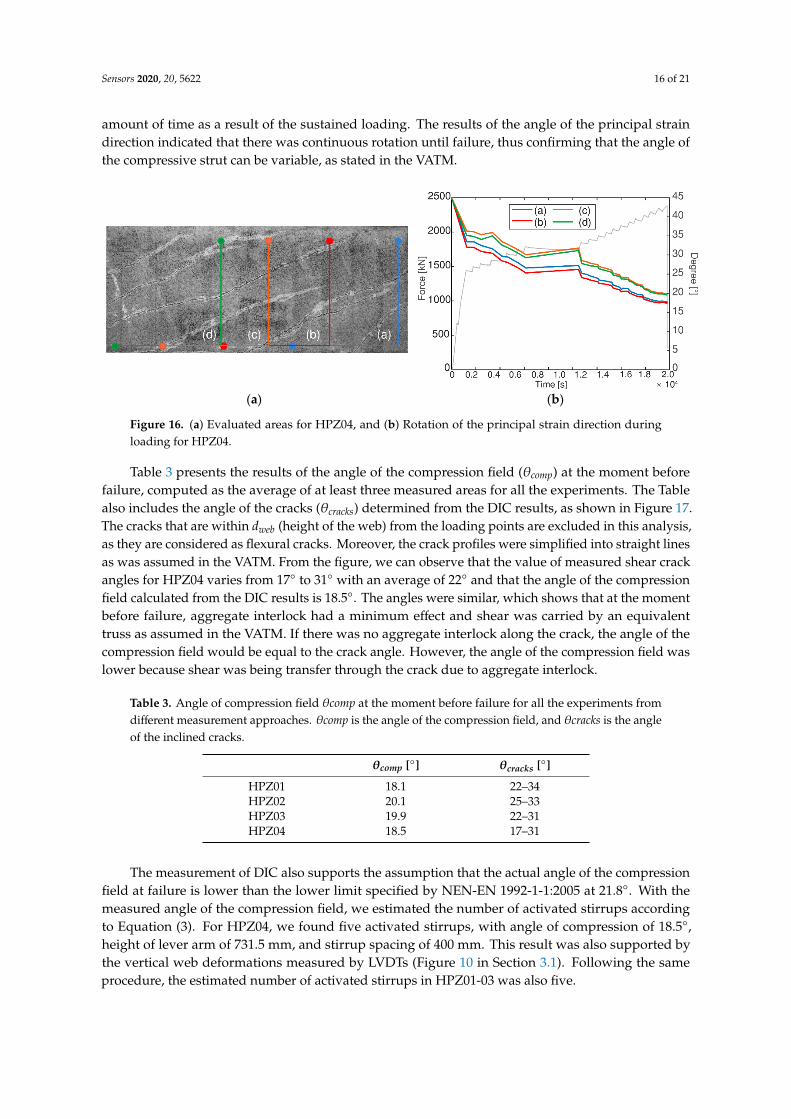
The angle of the compression field θwas calculated from the strain measurements as a function ofthe load. Figure 16a shows the four areas that were analyzed with the DIC algorithm and Figure 16bpresents the resulting angle as a function of time and the applied load for HPZ04. The generaltendency was that before cracking the principal strain direction was approximately 45◦. Then, after thedevelopment of the first inclined crack, the stiffness changes and the principal strain direction rotatedto a lower angle. The angle tended to increase slightly when the load was held for a considerable

Sensors 2020, 20, 5622 16 of 21

amount of time as a result of the sustained loading. The results of the angle of the principal straindirection indicated that there was continuous rotation until failure, thus confirming that the angle ofthe compressive strut can be variable, as stated in the VATM.


the development of the first inclined crack, the stiffness changes and the principal strain direction rotated to a lower angle. The angle tended to increase slightly when the load was held for a considerable amount of time as a result of the sustained loading. The results of the angle of the principal strain direction indicated that there was continuous rotation until failure, thus confirming that the angle of the compressive strut can be variable, as stated in the VATM.

(a) (b)

Figure 16. (a) Evaluated areas for HPZ04, and (b) Rotation of the principal strain direction during loading for HPZ04.

Table 3 presents the results of the angle of the compression field (θcomp) at the moment before failure, computed as the average of at least three measured areas for all the experiments. The Table also includes the angle of the cracks (θcracks) determined from the DIC results, as shown in Figure 17. The cracks that are within dweb (height of the web) from the loading points are excluded in this analysis, as they are considered as flexural cracks. Moreover, the crack profiles were simplified into straight lines as was assumed in the VATM. From the figure, we can observe that the value of measured shear crack angles for HPZ04 varies from 17° to 31° with an average of 22° and that the angle of the compression field calculated from the DIC results is 18.5°. The angles were similar, which shows that at the moment before failure, aggregate interlock had a minimum effect and shear was carried by an equivalent truss as assumed in the VATM. If there was no aggregate interlock along the crack, the angle of the compression field would be equal to the crack angle. However, the angle of the compression field was lower because shear was being transfer through the crack due to aggregate interlock.

Figure 17. Crack pattern and crack angle from DIC results of HPZ04.

Table 3. Angle of compression field θcomp at the moment before failure for all the experiments from different measurement approaches. θcomp is the angle of the compression field, and θcracks is the angle of the inclined cracks.

θcomp [°] θcracks [°] HPZ01 18.1 22–34 HPZ02 20.1 25–33

Figure 16. (a) Evaluated areas for HPZ04, and (b) Rotation of the principal strain direction duringloading for HPZ04.

Table 3 presents the results of the angle of the compression field (θcomp) at the moment beforefailure, computed as the average of at least three measured areas for all the experiments. The Tablealso includes the angle of the cracks (θcracks) determined from the DIC results, as shown in Figure 17.The cracks that are within dweb (height of the web) from the loading points are excluded in this analysis,as they are considered as flexural cracks. Moreover, the crack profiles were simplified into straight linesas was assumed in the VATM. From the figure, we can observe that the value of measured shear crackangles for HPZ04 varies from 17◦ to 31◦ with an average of 22◦ and that the angle of the compressionfield calculated from the DIC results is 18.5◦. The angles were similar, which shows that at the momentbefore failure, aggregate interlock had a minimum effect and shear was carried by an equivalenttruss as assumed in the VATM. If there was no aggregate interlock along the crack, the angle of thecompression field would be equal to the crack angle. However, the angle of the compression field waslower because shear was being transfer through the crack due to aggregate interlock.

Table 3. Angle of compression field θcomp at the moment before failure for all the experiments fromdifferent measurement approaches. θcomp is the angle of the compression field, and θcracks is the angleof the inclined cracks.

θcomp [◦] θcracks [◦]

HPZ01 18.1 22–34HPZ02 20.1 25–33HPZ03 19.9 22–31HPZ04 18.5 17–31

The measurement of DIC also supports the assumption that the actual angle of the compressionfield at failure is lower than the lower limit specified by NEN-EN 1992-1-1:2005 at 21.8◦. With themeasured angle of the compression field, we estimated the number of activated stirrups accordingto Equation (3). For HPZ04, we found five activated stirrups, with angle of compression of 18.5◦,height of lever arm of 731.5 mm, and stirrup spacing of 400 mm. This result was also supported bythe vertical web deformations measured by LVDTs (Figure 10 in Section 3.1). Following the sameprocedure, the estimated number of activated stirrups in HPZ01-03 was also five.

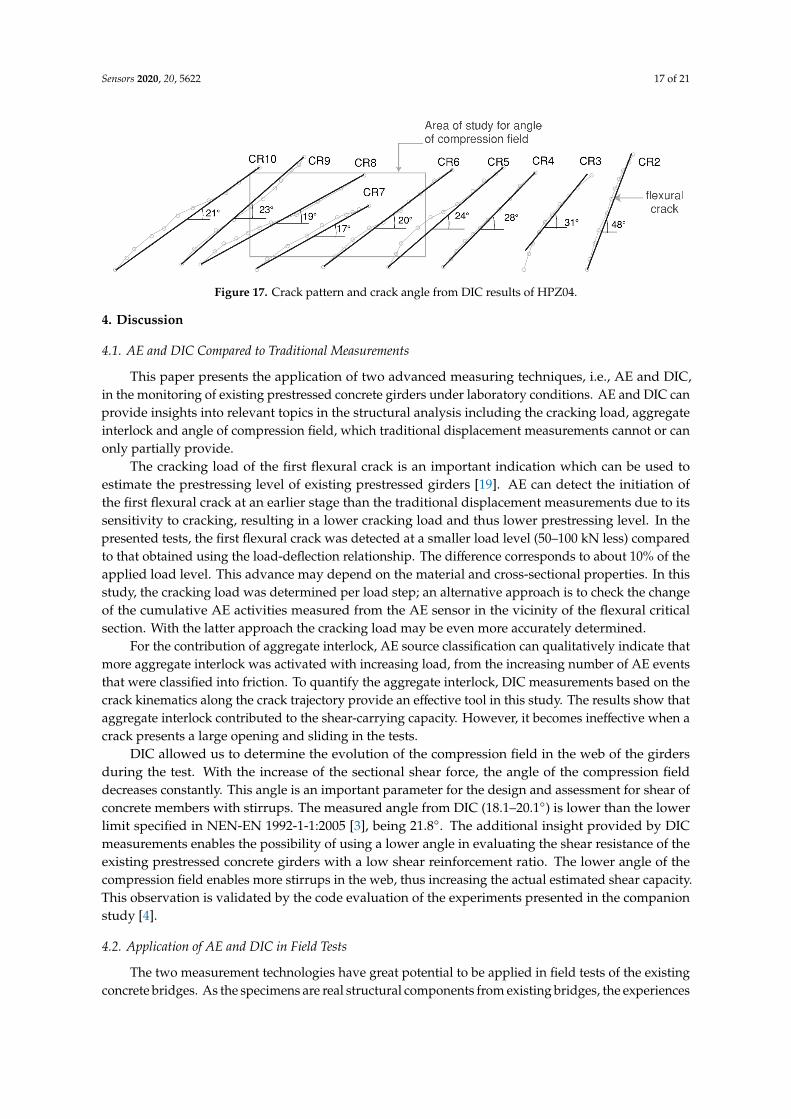
Sensors 2020, 20, 5622 17 of 21


the development of the first inclined crack, the stiffness changes and the principal strain direction rotated to a lower angle. The angle tended to increase slightly when the load was held for a considerable amount of time as a result of the sustained loading. The results of the angle of the principal strain direction indicated that there was continuous rotation until failure, thus confirming that the angle of the compressive strut can be variable, as stated in the VATM.

(a) (b)

Figure 16. (a) Evaluated areas for HPZ04, and (b) Rotation of the principal strain direction during loading for HPZ04.

Table 3 presents the results of the angle of the compression field (θcomp) at the moment before failure, computed as the average of at least three measured areas for all the experiments. The Table also includes the angle of the cracks (θcracks) determined from the DIC results, as shown in Figure 17. The cracks that are within dweb (height of the web) from the loading points are excluded in this analysis, as they are considered as flexural cracks. Moreover, the crack profiles were simplified into straight lines as was assumed in the VATM. From the figure, we can observe that the value of measured shear crack angles for HPZ04 varies from 17° to 31° with an average of 22° and that the angle of the compression field calculated from the DIC results is 18.5°. The angles were similar, which shows that at the moment before failure, aggregate interlock had a minimum effect and shear was carried by an equivalent truss as assumed in the VATM. If there was no aggregate interlock along the crack, the angle of the compression field would be equal to the crack angle. However, the angle of the compression field was lower because shear was being transfer through the crack due to aggregate interlock.


Table 3. Angle of compression field θcomp at the moment before failure for all the experiments from different measurement approaches. θcomp is the angle of the compression field, and θcracks is the angle of the inclined cracks.

θcomp [°] θcracks [°] HPZ01 18.1 22–34 HPZ02 20.1 25–33


4. Discussion

4.1. AE and DIC Compared to Traditional Measurements

This paper presents the application of two advanced measuring techniques, i.e., AE and DIC,in the monitoring of existing prestressed concrete girders under laboratory conditions. AE and DIC canprovide insights into relevant topics in the structural analysis including the cracking load, aggregateinterlock and angle of compression field, which traditional displacement measurements cannot or canonly partially provide.

The cracking load of the first flexural crack is an important indication which can be used toestimate the prestressing level of existing prestressed girders [19]. AE can detect the initiation ofthe first flexural crack at an earlier stage than the traditional displacement measurements due to itssensitivity to cracking, resulting in a lower cracking load and thus lower prestressing level. In thepresented tests, the first flexural crack was detected at a smaller load level (50–100 kN less) comparedto that obtained using the load-deflection relationship. The difference corresponds to about 10% of theapplied load level. This advance may depend on the material and cross-sectional properties. In thisstudy, the cracking load was determined per load step; an alternative approach is to check the changeof the cumulative AE activities measured from the AE sensor in the vicinity of the flexural criticalsection. With the latter approach the cracking load may be even more accurately determined.

For the contribution of aggregate interlock, AE source classification can qualitatively indicate thatmore aggregate interlock was activated with increasing load, from the increasing number of AE eventsthat were classified into friction. To quantify the aggregate interlock, DIC measurements based on thecrack kinematics along the crack trajectory provide an effective tool in this study. The results show thataggregate interlock contributed to the shear-carrying capacity. However, it becomes ineffective when acrack presents a large opening and sliding in the tests.

DIC allowed us to determine the evolution of the compression field in the web of the girdersduring the test. With the increase of the sectional shear force, the angle of the compression fielddecreases constantly. This angle is an important parameter for the design and assessment for shear ofconcrete members with stirrups. The measured angle from DIC (18.1–20.1◦) is lower than the lowerlimit specified in NEN-EN 1992-1-1:2005 [3], being 21.8◦. The additional insight provided by DICmeasurements enables the possibility of using a lower angle in evaluating the shear resistance of theexisting prestressed concrete girders with a low shear reinforcement ratio. The lower angle of thecompression field enables more stirrups in the web, thus increasing the actual estimated shear capacity.This observation is validated by the code evaluation of the experiments presented in the companionstudy [4].

4.2. Application of AE and DIC in Field Tests

The two measurement technologies have great potential to be applied in field tests of the existingconcrete bridges. As the specimens are real structural components from existing bridges, the experiences

Sensors 2020, 20, 5622 18 of 21

that have been learned from the test program can be extended to actual field tests. These applicationsare further discussed in this section.

The design of the AE measurement, especially the sensor layout, needs to consider various aspectsincluding the structural type, the material properties, the number of available sensors, and the size ofthe measuring area. For example, on-site measurements usually deal with large-size structures. With alimited number of AE sensors, it is suggested to first determine the interesting area, which could be thearea with the largest moment or the area critical to shear cracking. In this way, we reduce the size of themeasuring area and can install more AE sensors with less sensor spacing, which limits the influence ofwave travel distance on the AE signals. In the next step, within the interesting measuring area, it issuggested to do a measurement on the wave transfer properties of the concrete medium includingthe wave speed and attenuation. This step is essential as these properties may vary with differentstructures and change over the course of the service life [41]. With the measured wave attenuationproperty, we can determine the maximum distance that allows signals to be detected by the sensors.In a previous study on reinforced concrete elements, a sensor spacing of 0.5 m showed to be sufficientfor crack detection in reinforced concrete beams [29]. This sensor spacing was also found sufficient formonitoring the prestressed concrete girders in this paper. Only at the later stage near failure, the crackspacing got smaller in the web, it was then difficult for AE to distinguish those cracks. A solutioncould be to install AE sensors with less sensor spacing.

The design of the DIC setup in these experiments included three cameras with different focal lens.This is beneficial for the measurements of large-scale structures. The wide-angle lens camera allows usto capture a large measuring area, while the macro lens cameras provide detailed information in thecritical area. Further improvements on the accuracy of the measurements could be achieved by usinghigher resolution cameras for all the measuring areas or improve the speckle pattern and size.

Although the tested specimens in this paper were of real size, they were still tested in the laboratorywithin a couple of hours (maximum two days). For long-term monitoring of a real bridge, a few morechallenges need to be considered. First, environmental factors, such as rain and wind, may weakenthe coupling between the AE sensor and the bridge surface. Under this circumstance, long-term AEmonitoring requires effective protection of the sensors. For example, a protection box coving thesensors may be needed. DIC is affected by environmental factors, such as the change of lighting,which may affect the accuracy of the measurements. Other additional challenges are the preparationof the surface, the calibration of the cameras, and available camera locations. Then, as DIC needsa high-resolution camera, which is expensive, the DIC camera also requires protection. Moreover,the interesting area may not be accessible for DIC painting or AE sensor installation. In this case,for DIC, some researchers used the natural texture of the concrete (without painting patterns) [42].While this paper shows promising results for the use of these techniques, validation through researchstudies in the field will be necessary before commercial deployment is possible.

5. Conclusions

This article deals with the results obtained in the shear tests on four post-tensioned prestressedconcrete girders. These girders were heavily instrumented in the laboratory with traditionaldisplacement sensors, acoustic emission (AE) sensors, and cameras for analysis of the photographsusing digital image correlation (DIC).

AE could capture cracking before the traditional measurements and DIC, as AE is sensitive tocracking. In addition, the AE results have been used to identify the flexural cracking load of the girders,to derive the position of the cracks, and to identify the source of cracking (tensile cracking or friction).

The DIC algorithm gives further insight in the structural behavior of post-tensioned girdersfailing in shear. The visualization of the crack pattern helps in identifying the sequence of crackdevelopment. Studying the crack kinematics gives insight in the contribution of aggregate interlockas a shear-carrying mechanism. Moreover, analyzing the strains with Mohr’s circle shows that thecompression field rotates from 45◦ before cracking down to 18.1–20.1◦ at failure.

Sensors 2020, 20, 5622 19 of 21

For the assessment of shear-critical post-tensioned girders, insights from AE and DIC help tobetter understand the shear-transfer mechanisms, including aggregate interlock and the contributionof the stirrups. The results confirm that aggregate interlock contributes to the shear capacity, but withlarger crack openings, other mechanisms take over, which could be the shear-carrying capacity of thestirrups or the direct compression strut from the load to the support. The contribution of stirrups can beestimated from the DIC measurement of the angle of compression field. The angle of the compressionfield measured by DIC is smaller than that prescribed in the design code based on the VATM.

Ultimately, the combination of AE and DIC gives valuable insights in the cracking andshear-carrying behavior of prestressed concrete girders. This method could also be used for long-termmonitoring in the field, but further studies would be necessary to check the environmental influenceson the functioning of the sensors.

Author Contributions: Conceptualization, Y.Y. and E.L.; methodology, F.Z. and G.I.Z.G.; software, F.Z. andG.I.Z.G.; validation, Y.Y., E.L. and H.S.; formal analysis, F.Z. and G.I.Z.G.; investigation, F.Z. and G.I.Z.G.;resources, H.S.; data curation, F.Z. and G.I.Z.G.; writing—original draft preparation, E.O.L.L., F.Z. and G.I.Z.G.;writing—review and editing, Y.Y. and H.S.; visualization, F.Z. and G.I.Z.G.; supervision, Y.Y. and E.L.; projectadministration, Y.Y.; funding acquisition, Y.Y. All authors have read and agreed to the published version ofthe manuscript.

Funding: This research was funded by Rijkswaterstaat, the Dutch Ministry of Infrastructure and WaterManagement. The APC was funded by Delft University of Technology.

Acknowledgments: The authors wish to express their gratitude and sincere appreciation to the Dutch Ministry ofInfrastructure and Water Management (Rijkswaterstaat) for financing this research work. We are deeply indebtedto our colleague Albert Bosman for his work in the laboratory, development of the method to handle the girders,and design of the test setup. Thanks to Jakub Pawlowicz for his work in the laboratory, and for managing thematerial testing. Many thanks to our colleague Marco Roosen for the preparatory calculations, to René Braamand Cor van der Veen for starting this research project and for their invaluable advice during the preparationand testing stages of this series of experiments, to MSc thesis student Jayant Srivastava for helping with AcousticEmission measurement, and to former MSc thesis students Nikhil Jayananda, Shozab Mustafa, and Jos Migalskifor their prediction calculations.

Conflicts of Interest: The authors declare no conflict of interest.

References

1. Lantsoght, E.O.L.; Koekkoek, R.; van der Veen, C.; Sliedrecht, H. Fatigue Assessment of Prestressed ConcreteSlab-Between-Girder Bridges. Appl. Sci. 2019, 9, 2312. [CrossRef]

2. Roosen, M.; van der Veen, C.; Hordijk, D. Suitability of Shear Tension Code Requirements for the Assessmentof Existing Structures Build-Up with Prestressed I-and T-Shape Girders. High Tech Concrete: WhereTechnology and Engineering Meet. In Proceedings of the 2017 fib Symposium, Maastricht, The Netherlands,12–14 June 2017; pp. 786–793.

3. CEN European Committee for Standardization. EN 1992-1-1:2004. Eurocode 2: Design of ConcreteStructures—Part 1-1 General Rules and Rules for Buildings; CEN European Committee for Standardization:Brussels, Belgium, 2005; pp. 83–117.

4. Lantsoght, E.O.L.; Zarate Garnica, G.; Zhang, F.; Yang, Y.; Park, M.; Sliedrecht, H. Shear experiments ofprestressed concrete bridge girders. ACI Struct. J.. under review.

5. Park, M.; Lantsoght, E.O.L.; Zarate Garnica, G.; Yang, Y.; Sliedrecht, H. Analysis of Shear Capacity ofPrestressed Concrete Bridge Girders. ACI Struct. J.. under review.

6. Zhang, F.; Pahlavan, L.; Yang, Y. Evaluation of acoustic emission source localization accuracy in concretestructures. Struct. Health Monit. 2020, 1475921720915625. [CrossRef]

7. Kundu, T. Acoustic source localization. Ultrasonics 2013, 54, 25–38. [CrossRef]8. Ohtsu, M. Recommendation of RILEM TC 212-ACD: Acoustic emission and related NDE techniques for

crack detection and damage evaluation in concrete: Test method for classification of active cracks in concretestructures by acoustic emission. Mater. Struct. Mater. Constr. 2010, 43, 1187–1189. [CrossRef]

9. Soulioti, D.; Barkoula, N.M.; Paipetis, A.; Matikas, T.E.; Shiotani, T.; Aggelis, D.G. Acoustic emission behaviorof steel fibre reinforced concrete under bending. Constr. Build. Mater. 2009, 23, 3532–3536. [CrossRef]

http://dx.doi.org/10.3390/app9112312

http://dx.doi.org/10.1177/1475921720915625

http://dx.doi.org/10.1016/j.ultras.2013.06.009

http://dx.doi.org/10.1617/s11527-010-9640-6

http://dx.doi.org/10.1016/j.conbuildmat.2009.06.042

Sensors 2020, 20, 5622 20 of 21

10. Van Steen, C.; Pahlavan, L.; Wevers, M.; Verstrynge, E. Localisation and characterisation of corrosion damagein reinforced concrete by means of acoustic emission and X-ray computed tomography. Constr. Build. Mater.2019, 197, 21–29. [CrossRef]

11. Campana, S.; Fernández Ruiz, M.; Anastasi, A.; Muttoni, A. Analysis of shear-transfer actions on one-wayRC members based on measured cracking pattern and failure kinematics. Mag. Concr. Res. 2013, 65, 386–404.[CrossRef]

12. Huber, P.; Huber, T.; Kollegger, J. Investigation of the shear behavior of RC beams on the basis of measuredcrack kinematics. Eng. Struct. 2016, 113, 41–58. [CrossRef]

13. Cavagnis, F.; Fernández Ruiz, M.; Muttoni, A. An analysis of the shear-transfer actions in reinforced concretemembers without transverse reinforcement based on refined experimental measurements. Struct. Concr.2018, 19, 49–64. [CrossRef]

14. De Wilder, K.; Lava, P.; Debruyne, D.; Wang, Y.; De Roeck, G.; Vandewalle, L. Experimental investigation onthe shear capacity of prestressed concrete beams using digital image correlation. Eng. Struct. 2015, 82, 82–92.[CrossRef]

15. Gencturk, B.; Hossain, K.; Kapadia, A.; Labib, E.; Mo, Y.-L. Use of digital image correlation technique infull-scale testing of prestressed concrete structures. Measurement 2014, 47, 505–515. [CrossRef]

16. Schmidt, J.W.; Hansen, S.G.; Barbosa, R.A.; Henriksen, A. Novel shear capacity testing of ASR damaged fullscale concrete bridge. Eng. Struct. 2014, 79, 365–374. [CrossRef]

17. McCormick, N.J.; Lord, J.D. Practical In Situ Applications of DIC for Large Structures. Appl. Mech. Mater.2010, 24, 161–166. [CrossRef]

18. Schacht, G.; Bolle, G.; Marx, S. Experimental in-situ investigation of the shear bearing capacity of pre-stressedhollow core slabs. In Concrete Repair, Rehabilitation and Retrofitting IV; CRC Press: London, UK, 2015;pp. 851–859. [CrossRef]

19. ACI Committee 318. Building Code Requirements for Structural Concrete (ACI 318-14) and Commentary; AmericanConcrete Institute: Farmington Hills, MI, USA, 2014; p. 503.

20. Higgs, A.; Barr, P.J.; Halling, M.W. Comparison of Measured and AASHTO LRFD-Predicted ResidualPrestress Forces, Shear and Flexural Capacities of High-Strength Prestressed-Concrete Bridge Girders.J. Bridge Eng. 2015, 20, 05014009. [CrossRef]

21. Vecchio, F.; Collins, M.P. The modified compression-field theory for reinforced elements subjected to shear.ACI J. 1986, 83, 219–231.

22. AASHTO. LRFD Bridge Design Specifications and Commentary; Fourth edition with 2008 interim revisions;American Association of State Highway and Transportation Officials: Washington, DC, USA, 2008.

23. fib. Model Code 2010: Final Draft; International Federation for Structural Concrete: Lausanne, Switzerland,2012.

24. Walraven, J.C. Aggregate Interlock; Delft University Press: Delft, The Netherland, 1980.25. Nielsen, M.P.; Hoang, L.C. Limit Analysis and Concrete Plasticity; CRC Press: Boca Raton, USA, 2016.26. Physical Acoustics. R6I-AST Sensor. 2008. Available online: https://www.physicalacoustics.com/by-product/

sensors/R6I-AST-60-kHz-Integral-Preamp-AE-Sensor (accessed on 30 September 2020).27. Aggelis, D.G.; Shiotani, T.; Papacharalampopoulos, A.; Polyzos, D. The influence of propagation path

on elastic waves as measured by acoustic emission parameters. Struct. Health Monit. 2011, 11, 359–366.[CrossRef]

28. Polyzos, D.; Papacharalampopoulos, A.; Shiotani, T.; Aggelis, D.G. Dependence of AE parameters on thepropagation distance. J. Acoust. Emiss. 2011, 29, 57–67.

29. Zhang, F.; Yang, Y. Acoustic Emission based Crack Tracking for Existing Concrete Structural Members.In Proceedings of the 9th International Conference on Acoustic Emission, Chicago, IL, USA, 17–20 June 2019.

30. Pahlavan, L.; Zhang, F.; Blacquière, G.; Yang, Y.; Hordijk, D. Interaction of Ultrasonic Waves withPartially-closed Cracks in Concrete Structures. Constr. Build. Mater. 2018, 167, 899–906. [CrossRef]

31. Zhang, F. Evaluation of Acoustic Emission Monitoring of Existing Concrete Structures. Master’s Thesis,Delft University of Technology, Delft, The Netherlands, 2017.

32. Kurz, J.H.; Grosse, C.U.; Reinhardt, H.-W. Strategies for reliable automatic onset time picking of acousticemissions and of ultrasound signals in concrete. Ultrasonics 2005, 43, 538–546. [CrossRef] [PubMed]

33. Grosse, C.; Ohtsu, M. Acoustic Emission Testing: Basics for Research-Applications in Civil Engineering; Springer:Berlin, Germany, 2008; pp. 1–404. [CrossRef]


http://dx.doi.org/10.1680/macr.12.00142

http://dx.doi.org/10.1016/j.engstruct.2016.01.025

http://dx.doi.org/10.1002/suco.201700145


http://dx.doi.org/10.1016/j.measurement.2013.09.018


http://dx.doi.org/10.4028/www.scientific.net/AMM.24-25.161

http://dx.doi.org/10.1201/b18972-121

http://dx.doi.org/10.1061/(ASCE)BE.1943-5592.0000646

https://www.physicalacoustics.com/by-product/sensors/R6I-AST-60-kHz-Integral-Preamp-AE-Sensor

https://www.physicalacoustics.com/by-product/sensors/R6I-AST-60-kHz-Integral-Preamp-AE-Sensor

http://dx.doi.org/10.1177/1475921711419992


http://dx.doi.org/10.1016/j.ultras.2004.12.005

http://www.ncbi.nlm.nih.gov/pubmed/15950028

http://dx.doi.org/10.1007/978-3-540-69972-9

Sensors 2020, 20, 5622 21 of 21

34. Ohtsu, M.; Uchida, M.; Okamoto, T.; Yuyama, S. Damage assessment of reinforced concrete beams qualifiedby acoustic emission. ACI Struct. J. 2002, 99, 411–417.

35. Pan, B.; Xie, H.; Guo, Z.; Hua, T. Full-field strain measurement using a two-dimensional Savitzky-Golaydigital differentiator in digital image correlation. Opt. Eng. 2007, 46. [CrossRef]

36. Jones, E. Documentation for Matlab-Based DIC Code; Urbana-Champaign, University of Illinois:Urbana-Champaign, IL, USA, 2015.

37. Zarate, G. Analysis of shear transfer mechanisms in concrete members without shear reinforcement basedon kinematic measurements. Master’s Thesis, TU Delft, Delft, The Netherlands, 2018.

38. Amiot, F.; Bornert, M.; Doumalin, P.; Dupré, J.C.; Fazzini, M.; Orteu, J.J.; Poilâne, C.; Robert, L.; Rotinat, R.;Toussaint, E.; et al. Assessment of Digital Image Correlation Measurement Accuracy in the Ultimate ErrorRegime: Main Results of a Collaborative Benchmark. Strain 2013, 49, 483–496. [CrossRef]

39. Barranger, Y.; Doumalin, P.; Dupré, J.C.; Germaneau, A. Digital Image Correlation accuracy: Influence ofkind of speckle and recording setup. EPJ Web Conf. 2010, 6. [CrossRef]

40. Walraven, J.C. Fundamental Analysis of Aggregate Interlock. ASCE J. Struct. Div. 1981, 107, 2245–2270.41. Van Steen, C.; Zhang, F.; Nasser, H.; Yang, Y.; Verstrynge, E. On-site inspection of a reinforced concrete

structure deteriorated due to corrosion by means of acoustic emission and other techniques. In Proceedingsof the Conference: Structural Faults and Repair 2018, Edinburgh, UK, 15–17 May 2018.

42. Schmidt, J.W.; Halding, P.S.; Jensenm, T.W.; Engelund, S. High Magnitude Loading of Concrete Bridges.ACI Symp. Publ. 2018, 323, 9.1–9.20.

© 2020 by the authors. Licensee MDPI, Basel, Switzerland. This article is an open accessarticle distributed under the terms and conditions of the Creative Commons Attribution(CC BY) license (http://creativecommons.org/licenses/by/4.0/).

http://dx.doi.org/10.1117/1.2714926

http://dx.doi.org/10.1111/str.12054

http://dx.doi.org/10.1051/epjconf/20100631002

http://creativecommons.org/

http://creativecommons.org/licenses/by/4.0/.

Documents

Monitoring Shear Behavior of Prestressed Concrete Bridge