MORSE’S INDEX FORMULA IN VMO

FOR COMPACT MANIFOLDS WITH BOUNDARY

GIACOMO CANEVARI, ANTONIO SEGATTI, AND MARCO VENERONI

Abstract. In this paper, we study Vanishing Mean Oscillation vector fields on a compactmanifold with boundary. Inspired by the work of Brezis and Niremberg, we construct a

topological invariant — the index — for such fields, and establish the analogue of Morse’s

formula. As a consequence, we characterize the set of boundary data which can be extended tonowhere vanishing VMO vector fields. Finally, we show briefly how these ideas can be applied

to (unoriented) line fields with VMO regularity, thus providing a reasonable framework for

modelling a surface coated with a thin film of nematic liquid crystals.

1. Introduction

The starting point of the investigations developed in this paper is the analysis of a variationalmodel for nematic shells. Nematic shells are the datum of a two-dimensional surface (for simplic-ity, at a first step, without boundary) N ⊂ R3 coated with a thin film of nematic liquid crystal([16, 18, 21, 22, 23, 27, 28, 30]). This line of research has attracted a lot of attention from thephysics community due to its vast technological applications (see [23]). From the mathematicalpoint of view, nematic shells offer an interesting and nontrivial interplay between calculus ofvariations, partial differential equations, geometry and topology. The basic mathematical de-scription of nematic shells consists in an energy defined on tangent vector fields with unit length,named directors. This energy, in the simplest situation, takes the form

(1.1) E(n) :=

ˆN

|∇n|2dS,

where ∇ stands for the covariant derivative of the surface N . If one is interested in the min-imization of this energy, the first step is to understand whether there are competitors for theminimization process. For this type of energy, the natural functional space where to look forminimizers is the space of tangent vector fields with H1 regularity. This means, recalling thatwe are looking for vector fields with unit norm, the space defined in this way

(1.2) H1tan(N, S2) :=

n ∈ H1(N, R3) : n(x) ∈ Tx(N) and |n| = 1 a.e.

.

Now, the problem turns into the understanding of the topological conditions on N , if any, thatmake H1

tan(N, S2) empty or not. Note that this problem, in the case N = S2, is indeed a Sobolevversion of the celebrated hairy ball problem concerning the existence of a tangent vector fieldwith unit norm on the two-dimensional sphere. The answer, when dealing with continuous fields,is negative. This is a consequence of a more general result, the Poincare-Hopf Theorem, thatrelates the existence of a smooth tangent vector field with unit norm to the topology of N . Moreprecisely, a smooth vector field with unit norm exists if and only if χ(N) = 0, where χ is theEuler characteristic of N . In case N is a compact surface in R3, the Euler characteristic can bewritten as a function of the topological genus k:

χ(N) = 2(1− k).

Date: July 7, 2014.2010 Mathematics Subject Classification. 55M25, 57R25, 53Z05, 76A15.Key words and phrases. Index of a vector field, VMO degree theory, Poincare-Hopf-Morse’s formula, Q-tensors.

1

arX

iv:1

407.

1707

v1 [

mat

h.FA

] 7

Jul

201

4

2 GIACOMO CANEVARI, ANTONIO SEGATTI, AND MARCO VENERONI

In [27] it has been proved, using calculus of variations tools, that the very same result holds forvector fields with H1 regularity. Therefore, up to diffeomorphisms, the only compact surface inR3 which admits a unit norm vector field in H1 is the torus, corresponding to k = 1. On theother hand, it is easy to comb the sphere with a field v ∈ W 1,p

tan(S2, S2) for all 1 ≤ p < 2. It isinteresting to note that this result could be seen as a ”non flat” version of a well know result ofBethuel that gives conditions for the non emptiness of the space

H1g (Ω;S1) :=

v ∈ H1(Ω;R2) : |v(x)| = 1 a.e. in Ω and v ≡ g on ∂Ω

,

where Ω is a simply connected bounded domain in R2 and g is a prescribed smooth boundarydatum with |g| = 1. The non-emptiness of H1

g (Ω; S1) is related to a topological condition on theDirichlet datum g (see [2] and [3]) while in the result in [27] the topological constraint is on thegenus of the surface.

Instead of using the standard Sobolev theory, we reformulate this problem in the space ofVanishing Mean Oscillation (VMO) functions, introduced by Sarason in [26], which constitute aspecial subclass of Bounded Mean Oscillations functions, defined by John and Niremberg in [15].We recall the definitions and some properties of these objects in Section 2, but we immediatelynote that VMO contains the critical spaces with respect to Sobolev embeddings, that is,

(1.3) W s,p(Rn) ⊂ VMO(Rn) when sp = n, 1 < s < n.

In a sense, VMO functions are a good surrogate for the continuous functions, because someclassical topological constructions can be extended, in a natural way, to the VMO setting. Inparticular, we recall here the VMO degree theory, which has been developed after Brezis andNiremberg’s seminal papers [4] and [5].

Besides relaxing the regularity on the vector field, we will consider n-dimensional compactand connected submanifolds of Rn+1 and, instead of fixing the length of the vector field to be 1,we will look for vector fields which are bounded and uniformly positive.

Thus, the problem of combing a two-dimensional surface with H1 vector fields can be gener-alized in the following way.

Question 1. Let N be a compact, connected submanifold of Rn+1, without boundary, of dimen-sion n. Does a vector field v ∈ VMO(N, Rn+1), satisfying

(1.4) v(x) ∈ TxN and c1 ≤ |v(x)| ≤ c2for a.e. x ∈ N and some constants c1, c2 > 0, exists?

The first outcome of this paper is to provide a complete answer to Question 1. By means ofthe Brezis and Niremberg’s degree theory, we can show that the existence of nonvanishing vectorfields in VMO is subject to the same topological obstruction as in the continuous case, that is,we prove the following

Proposition 1.1. Let N be a compact, connected submanifold of Rn+1, without boundary. Thereexists a function v ∈ VMO(N, Rn+1) satisfying (1.4) if and only if χ(N) = 0.

After addressing manifolds without boundary, we consider the case where N is a manifoldwith boundary, and we prescribe Dirichlet boundary conditions to the vector field v on N . Themain issue of this paper is to understand which are the topological conditions on the manifoldN and on the Dirichlet boundary datum that guarantee the existence of a nonvanishing andbounded tangent vector field on N extending the boundary condition. Applications of theseresults can be found in variational problems for vector fields that satisfy a prescribed boundarycondition of Dirichlet type, e.g., in the framework of liquid crystal shells.

More precisely, we address the following problem:

Question 2. Let N ⊂ Rd be a compact, connected and orientable n-submanifold with boundary.Let g : ∂N → Rd be a boundary datum in VMO, satisfying

(1.5) g(x) ∈ TxN and c1 ≤ |g(x)| ≤ c2

MORSE’S INDEX FORMULA IN VMO FOR MANIFOLDS WITH BOUNDARY 3

for Hn−1-a.e. x ∈ ∂N and some constants c1, c2 > 0. Does a field v ∈ VMO(N, Rd), whichfulfills (1.4) and has trace g (in some sense, to be specified), exist?

When working in the continuous setting, a similar issue can be investigated with the help ofa topological tool: the index of a vector field. In particular, even in this weak framework, weexpect conditions that relate the index of the boundary conditions with the index of the tangentvector field and the Euler characteristic of N . In order to understand the difficulties and to easethe presentation, we recall here some definitions related to the degree theory and an importantproperty.

First, we recall Brouwer’s definition of degree. Let N be as in Question 2 and let M be aconnected, orientable manifold without boundary, of the same dimension as N . Let ϕ : N →Mbe a smooth map, and let p ∈M \ϕ(∂N) be a regular value for ϕ (that is, the Jacobian matrixDϕ(x) is non-singular for all x ∈ ϕ−1(p)). We define the degree of ϕ with respect to p as

deg(ϕ, N, p) :=∑

x∈ϕ−1(p)

sign(detDϕ(x)).

This sum is finite, because ϕ−1(p) is a discrete set (as ϕ is locally invertible around each pointof ϕ−1(p)) and N is compact.

It can be proved that, if p1 and p2 are two regular values in the same component of M \ ϕ(∂N),then deg(ϕ, N, p1) = deg(ϕ, N, p2). Since the regular values of ϕ are dense in M (by Sardlemma), the definition of deg(ϕ, N, p) can be extended to every p ∈M \ ϕ(∂N). Moreover, byapproximation it is possible to the define the degree when ϕ is just continuous. In case N is amanifold without boundary, deg(ϕ, N, p) does not depend on the choice of p ∈ M , so we willdenote it by deg(ϕ, N, M). Let us mention also that, if N and M are compact and withoutboundary, the following formula holds:

(1.6) deg(ϕ, N, M) =1

τ(M)

ˆN

ϕ∗(dτ) =1

τ(M)

ˆN

detDϕ(x) dσ(x),

where σ, τ are the Riemannian metrics on N and M , respectively.Ideally, given a continuous vector field v, one would like to define its index by

ind(v, N) = deg(v, N, 0).

However, this is not possible, because in order to define the degree it is essential that the domainand the target manifold have the same dimension. This is not the case here, since the domainmanifold N ⊂ Rd has dimension strictly less that the target manifold Rd. To overcome this issue,there are at least two different strategies. The one we consider in this paper, which is also themost widely studied in the literature (see, e.g., [20, 10, 17, 19, 29]), is to use coordinate charts torepresent v, locally around its zeros, as a map Rn → Rn. This requires an additional assumption,namely that the zero set of v is discrete. Thus, within this approach, an approximation techniqueis needed in order to extend the definition of index to any continuous field. This construction,based on the Transversality Theorem, is explained in detail in Section 3. Another possibilityis to consider an open neighbourhood U ⊂ Rd of N , and extend v to a map w : U → Rd, in asuitable way. Then, it would make sense to write

ind(v, N) := deg(w, U, 0),

and this would give an equivalent definition of the index. This approach is inspired by a classicalproof of the Poincare-Hopf theorem, which can be found in [19, Theorem 1, p. 38]). Some detailsof this construction are given in Remark 3.4.

Once the index has been properly defined, it can been used to establish a precise relationbetween the behaviour of a vector field v and the topological properties of N . Denote by ∂−Nthe subset of the boundary where v points inward (that is, letting ν(x) be the outward unitnormal to ∂N in TxN , we have x ∈ ∂−N if and only if v(x) · ν(x) < 0). Call P∂Nv the vectorfield on ∂N defined by

P∂Nv(x) := projTx∂N v(x) for all x ∈ ∂N.

4 GIACOMO CANEVARI, ANTONIO SEGATTI, AND MARCO VENERONI

Morse proved the following equality (see [20]), which was later rediscovered and generalized byPugh (see [24]) and Gottlieb (see [8, 9]).

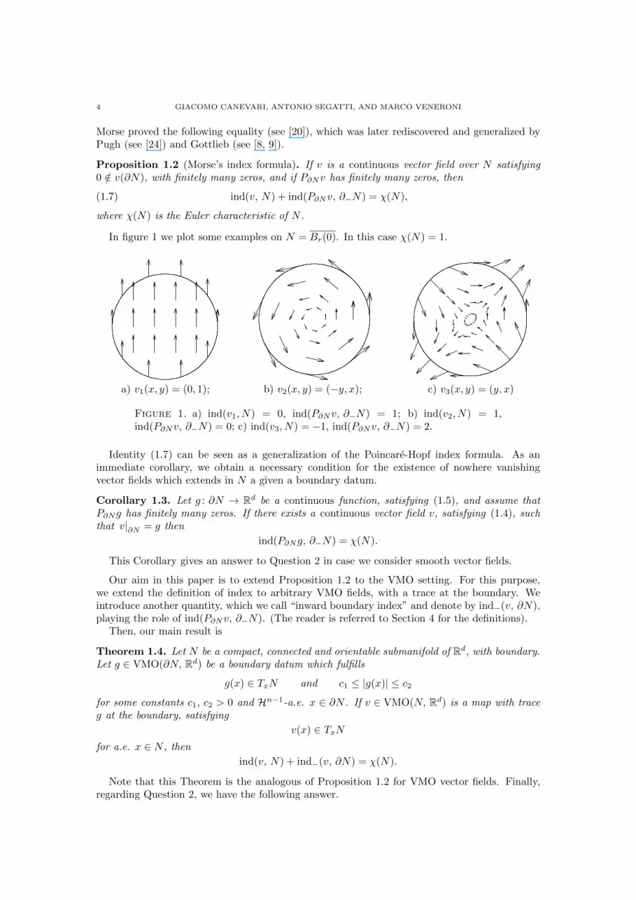
Proposition 1.2 (Morse’s index formula). If v is a continuous vector field over N satisfying0 /∈ v(∂N), with finitely many zeros, and if P∂Nv has finitely many zeros, then

(1.7) ind(v, N) + ind(P∂Nv, ∂−N) = χ(N),

where χ(N) is the Euler characteristic of N .

In figure 1 we plot some examples on N = Br(0). In this case χ(N) = 1.

a) v1(x, y) = (0, 1); b) v2(x, y) = (−y, x); c) v3(x, y) = (y, x)

Figure 1. a) ind(v1, N) = 0, ind(P∂Nv, ∂−N) = 1; b) ind(v2, N) = 1,ind(P∂Nv, ∂−N) = 0; c) ind(v3, N) = −1, ind(P∂Nv, ∂−N) = 2.

Identity (1.7) can be seen as a generalization of the Poincare-Hopf index formula. As animmediate corollary, we obtain a necessary condition for the existence of nowhere vanishingvector fields which extends in N a given a boundary datum.

Corollary 1.3. Let g : ∂N → Rd be a continuous function, satisfying (1.5), and assume thatP∂Ng has finitely many zeros. If there exists a continuous vector field v, satisfying (1.4), suchthat v|∂N = g then

ind(P∂Ng, ∂−N) = χ(N).

This Corollary gives an answer to Question 2 in case we consider smooth vector fields.

Our aim in this paper is to extend Proposition 1.2 to the VMO setting. For this purpose,we extend the definition of index to arbitrary VMO fields, with a trace at the boundary. Weintroduce another quantity, which we call “inward boundary index” and denote by ind−(v, ∂N),playing the role of ind(P∂Nv, ∂−N). (The reader is referred to Section 4 for the definitions).

Then, our main result is

Theorem 1.4. Let N be a compact, connected and orientable submanifold of Rd, with boundary.Let g ∈ VMO(∂N, Rd) be a boundary datum which fulfills

g(x) ∈ TxN and c1 ≤ |g(x)| ≤ c2for some constants c1, c2 > 0 and Hn−1-a.e. x ∈ ∂N . If v ∈ VMO(N, Rd) is a map with traceg at the boundary, satisfying

v(x) ∈ TxNfor a.e. x ∈ N , then

ind(v, N) + ind−(v, ∂N) = χ(N).

Note that this Theorem is the analogous of Proposition 1.2 for VMO vector fields. Finally,regarding Question 2, we have the following answer.

MORSE’S INDEX FORMULA IN VMO FOR MANIFOLDS WITH BOUNDARY 5

Proposition 1.5. Let g ∈ VMO(∂N, Rd) satisfy the assumption (1.5). A field v ∈ VMO(N, Rd)that satisfies (1.4) and has trace g exists if and only if

(1.8) ind−(g, ∂N) = χ(N).

We conclude this introduction with an outline of the paper. In Section 2 we provide somepreliminary material on the VMO space. Then, in Section 3 we introduce the notion of index fora continuous vector field, starting with the basic case of a field with a finite number of zeros andthen moving to an arbitrary number of zeros by Thom’s Transversality Theorem. In Section 4,by means of an approximation argument, this extension allows us to give a notion of index fora VMO vector field and to prove Theorem 1.4. Finally, in Section 5, we apply these results tothe existence of line fields with VMO regularity. Interestingly, such an existence result sharesthe same topological obstruction as the existence result for vector fields. As a side result of theexistence of VMO Q-tensor fields, we obtain topological conditions for the existence of line fieldswith VMO regularity, thus extending to this weaker setting a classical result due to Poincareand Kneser.

Notation. In the following sections either N = Rn, or N is a compact, connected and orientedmanifold with boundary, of dimension n, embedded as a submanifold of Rd for some d ∈ N.

- The injectivity radius of N (see, e.g., do Carmo [7]) is called r0.- We denote geodesic balls in N by BNr (x) or simply Br(x), when it is clear from the

context that we work in N . In case N = Rn, we write Bnr (x) or Bn(x, r).- For ε > 0, we set

Nε := x ∈ N : dist(x, ∂N) ≥ ε .- For each x ∈ ∂N , we denote by ν(x) the outward unit normal to ∂N in TxN .- Given a non-empty, convex and closed set K ⊂ Rd, we denote the nearest-point projec-

tion on K by projK .- Given a manifold X ⊂ Rd and a continuous map v : X → Rd, we denote the tangential

component of v by

PXv(x) := projTxXv(x) for x ∈ X.

2. Preliminary material: VMO functions

For the reader’s convenience, we recall here the basic definitions about VMO functions, fol-lowing the presentation of [5] (to which the reader is referred, for more details). All the functionswe consider here take values in Rd, so functional spaces such as, e.g., L1(N, Rd) or VMO(N, Rd)will be simply written as L1(N) or VMO(N).

Recall that N is endowed with a Riemannian measure σ. For u ∈ L1(N) (with respect to σ),define

(2.1) ‖u‖BMO := supε≤r0, x∈N2ε

Bε(x)

|u(y)− uε(x)| dσ(y),

where

(2.2) uε(x) :=

Bε(x)

u(y) dσ(y), for x ∈ N2ε.

The set of functions with ‖u‖BMO < +∞ will be denoted BMO(N), and (2.1) defines a norm onBMO(N) modulo constants. Using cubes instead of balls leads to an equivalent norm. Moreover,if ϕ : X1 → X2 is a C 1 diffeomorphism between two unbounded manifolds, then u ∈ BMO(X2)implies u ϕ ∈ BMO(X1) and

‖u ϕ‖BMO(X1)≤ C ‖u‖BMO(X2)

.

Bounded functions (in particular, continuous functions) belong to BMO. Following Sarason, wedefine VMO(N) as the closure of C (N) with respect to the BMO norm. Functions in VMO(N)can be characterized by means of this lemma (see [4, Lemma 3]):

6 GIACOMO CANEVARI, ANTONIO SEGATTI, AND MARCO VENERONI

Lemma 2.1. A function u ∈ BMO(N) is in VMO(N) if and only if

limε→0

supx∈N2ε

Bε(x)

|u(y)− uε(x)| dσ(y)→ 0.

Sobolev spaces provide an interesting class of functions in VMO, since, for critical exponents,the embeddings which fail to be in L∞ hold true in VMO:

W s,p(N) ⊂ VMO(N) whenever 0 < s < n, sp = n.

In general, VMO functions do not have a trace on the boundary. However, it is possible tointroduce a subclass of VMO for which traces are well defined. We sketch here the construction.

First, we need to embed N as a domain of a bigger manifold X, smooth and without boundary.Here, we take X as the double of N , that is, the manifold we obtain by gluing two copies of Nalong their boundaries. Modifying, if necessary, the value of d we can assume that X ⊂ Rd. Also,let U be a tubular neighbourhood of ∂N in X, and assume that the nearest-point projectionπ : U → ∂N is well defined. Now, we fix g ∈ VMO(∂N) and we extend it to a function G, bythe formula

(2.3) G(x) =

g(π(x))χ(x) if x ∈ X ∩ U0 if x ∈ X \ U

where χ is a cut-off function, which is equal to 1 near ∂N and vanishes outside U . It can bechecked that G ∈ VMO(X).

We say that a function u ∈ VMO(N) has trace g on ∂N , and we write u ∈ VMOg(N), if andonly if the function defined by

u in N

G in X \N

is in VMO(X). This definition is independent on the choice of χ and of X (see [5, Prop-erty 6]). The notion of VMOg is stable under diffeomorphism: suppose ϕ : X1 → X2 is aC 1 diffeomorphism between bounded manifolds, mapping diffeomorphically ∂X1 onto ∂X2 . Ifg ∈ VMO(∂X2) and u ∈ VMOg(X2), then

u ϕ ∈ VMOgϕ(X1).

As an example of VMO functions with trace, let us mention that every map in W 1,n(X) has atrace in the sense of VMO, which coincides with the Sobolev trace.

2.1. Combing an unbounded manifold in VMO. In this section, we prove Proposition 1.1.Of course, it could be obtained as a corollary of our main result, Theorem 1.4. Anyway, it canbe proved independently, and we present here an elementary argument inspired by [11, Theorem2.28]. We assume that N is a compact, connected n-manifold without boundary, embedded asan hypersurface of Rn+1.

Proof of Proposition 1.1. It is well-known that, if χ(N) = 0, then a nowhere vanishing, smooth(hence VMO) vector field on N exists. The idea of the proof is the following: One picks anarbitrary continuous field, approximates it with a field v having a finite number of zeros, thenuses the Poincare-Hopf formula and the hypothesis χ(N) = 0 to show that ind(v, N) = 0, so vcan be modified into a nowhere vanishing field. This argument is given in detail in the proof ofCorollary 1.5, in case N is a manifold with boundary, and it is even simpler when ∂N = ∅.

Let us prove the other side of the proposition: we suppose that a tangent vector fieldv ∈ VMO(N) such that ess infN |v| > 0 exists, and we claim that χ(N) = 0. Every compacthypersurface of Rn+1 is orientable, so there is a smooth unit vector field γ : N → Rn+1 such thatγ(x) ⊥ TxN for all x ∈ N . The choice of such a map induces an orientation on N , and γ is calledthe Gauss map of the oriented manifold N . We can also assume that n is even, since χ(N) = 0whenever N is a compact, unbounded manifold of odd dimension (see, e.g., [11, Corollary 3.37]).

MORSE’S INDEX FORMULA IN VMO FOR MANIFOLDS WITH BOUNDARY 7

Consider the function H : N × [0, π]→ Rn+1 given by

H(x, t) := (cos t)γ(x) + (sin t)v(x).

It is readily checked that |H(x, t)|2 = 1 for all (x, t) ∈ N × [0, π]. We claim that

(2.4) H ∈ C ([0, π], VMO(N, Sn)) .

Indeed, H(·, t) is the linear combination of functions in VMO(N) and hence belongs to VMO(N),for all t. On the other hand, for all t1, t2 ∈ [0, π]

‖H(·, t1)−H(·, t2)‖BMO ≤ |cos t1 − cos t2| ‖γ‖BMO + |sin t1 − sin t2| ‖v‖BMO ,

whence the claimed continuity (2.4) follows.Since the degree is a continuous function VMO(N, Sn) → Z (see [4, Theorem 1]), we infer

that

deg(H(·, 0), N, Sn) = deg(H(·, π), N, Sn).

On the other hand, H(·, 0) = γ and H(·, π) = −γ. By standard properties of the degree (inparticular, [11, Properties (d, f) p. 134]), and since we have assumed that n is even, we have

deg(−γ, N, Sn) = (−1)n+1 deg(γ, N, Sn) = −deg(γ, N, Sn),

hence

deg(γ, N, Sn) = − deg(γ, N, Sn).

By the degree formula (1.6) and Gauss-Bonnet Theorem (see, e.g., [10, page 196]), for an even-dimensional hypersurface N

deg(γ, N, Sn) = deg(γ, N, Sn)

Sn

dσn =1

ωn

ˆN

γ∗(dσn) =1

ωn

ˆN

κdσ =1

2χ(N),

where dσn is the volume form of Sn, ωn :=´Sn dσn is the volume of Sn, and κ is the Gaussian

curvature of N . Since deg(γ, N, Sn) = 0 by the above construction, this shows that χ(N) = 0and thus completes the proof.

Remark 2.2. When χ(N) 6= 0, Proposition 1.1 shows that there is no unit vector field in thecritical Sobolev space W s,p(N), for 0 < s < n and sp = n. In contrast, when sp < n it is notdifficult to construct unit vector fields in W s,p(N). For instance, on N = S2k one may considera field with two “hedgehog” singularities, of the form x 7→ x/ |x|, located at the opposite polesof the sphere.

3. The index of a continuous field

We aim to extend Morse formula to the VMO setting. As a preliminary step, we need to definethe index for any continuous vector field, dropping out the assumption of finitely many zeros.This goal can be achieved quite straightforwardly, by applying a fundamental tool of differentialgeometry: the transversality theorem. Such a construction is usually given for granted but,for the reader’s convenience, in this section we present it in detail. As a consequence of thetransversality theorem, we are able to extend some properties of the classical index of a vectorfield, namely excision, invariance under homotopy, and stability, to continuous vector fields withany number of zeros. In Propositions 3.5 and 3.6 and in Corollary 3.7 we give the correspondingstatements.

Let us start by recalling the definition of transversality. Throughout this section, we denoteby X ⊂ Rd a compact, connected and oriented manifold without boundary (in what followswe will take as X either the double of N or ∂N). Also, let E be a smooth manifold (withoutboundary), ϕ : X → E a map of class C 1, and Y ⊂ E a submanifold.

Definition 3.1. The map ϕ is said to be transverse to Y if and only if, for all x ∈ ϕ−1(Y ), wehave

dϕx(TxX)⊕ Tϕ(x)Y = Tϕ(x)E.

8 GIACOMO CANEVARI, ANTONIO SEGATTI, AND MARCO VENERONI

b

X

ϕ

E

Y

ϕ(X)

Figure 2. An example of transversality: The curve ϕ on the sphere E istransverse to the equator Y . Their tangent lines generate the tangent plane toE in the points of intersection.

In other words, we ask the image of ϕ to “cross transversally” the submanifold Y , at eachpoint of intersection. In our case of interest, E = TX is the tangent bundle of X, equipped withthe natural projection π : E → X given by (x, w) 7→ x. We take ϕ to be a section of π — thatis, a map ϕ : X → E such that π ϕ = IdX . Notice that given a vector field v : X → Rd, thereexists a unique section of π induced by v, that is

ϕ : x ∈ X 7→ (x, v(x)) ∈ E.

Vice-versa, each section of π induces a unique vector field X → Rd, because each tangent planeTxX ∈ E can be regarded as a hyperplane of Rd. Finally, we take Y as the image of the zerosection, that is,

Y := (x, 0) : x ∈ X ⊂ E.Clearly, Y is a submanifold of E, diffeomorphic to X, and ϕ(x) ∈ Y if and only if v(x) = 0.

Transverse sections can be characterized in terms of the corresponding vector fields. To do so,fix a point x ∈ X and a chart f : V → Rn in a neighbourhood of x. Then, define the (smooth)map f∗v : f(V ) ⊂ Rn → Rn by

f∗v(y) := dff−1(y)(v(f−1(y))) for all y ∈ f(V ) ⊂ Rn.

Since Tϕ(x)Y = TxM ⊕ 0, then ϕ is transverse to Y in x if and only if dϕx is invertible, i.e.,if and only if dvx is invertible. As

d(f∗v)f(x) = dfx dvx (dfx)−1,

we obtain the following

Proposition 3.1. The map ϕ is transverse to Y if and only if for all x ∈ v−1(0) the differentiald(f∗v)f(x) is invertible.

If f , g are two local charts around x, then d(f∗v)f(x) is invertible if and only if d(g∗v)g(x) is, sothis characterization is independent of the choice of the chart. Vector fields in these conditionswill simply be called transverse fields. Remark that, for a transverse field v, the set v−1(0)is discrete (by the local inversion theorem), hence is finite because X is compact. Moreover,given two coordinate charts f and g which agree with the fixed orientation of X, the Jacobians

MORSE’S INDEX FORMULA IN VMO FOR MANIFOLDS WITH BOUNDARY 9

det d(f∗v)f(x) and det d(g∗v)g(x) have the same sign. Thus, if U ⊂ X is an open set and v avector field on X satisfying

0 /∈ v(∂U),

the index of v on U is well-defined by the formula

(3.1) ind(v, U) :=∑

x∈v−1(0)∩U

sign det d(f∗v)f(x).

This formula can be expressed in an equivalent way. Pick a geodesic ball Br(x) ⊂⊂ U around

each zero x, so small that no other zero is contained in Br(x). Then, f∗v|f∗v| is well-defined as a

map ∂Br(x) ' Sn−1 → Sn−1, and

(3.2) ind(v, U) =∑

x∈v−1(0)∩U

deg

(f∗v

|f∗v|, ∂Br(x), Sn−1

).

The equivalence of (3.1) and (3.2) follows, e.g., from [5, Equation (4.1), p. 25].Since we want to extend the definition of index to any continuous field, it is natural to ask

whether a continuous field can be approximated by transverse fields. The transversality theoremgives a positive answer. This result, due to Thom (see [31, 32]), states that transverse mappingsare a dense subset of continuous mappings. The statement that we present here is [6, Theorem14.6]. This formulation is convenient for our purposes, because it guarantees that if ϕ is a sectionof π, then the approximating transverse maps can be chosen to be sections as well.

Theorem 3.2 (Transversality theorem). Let π : E → X be a smooth vector bundle, Y a sub-manifold of E, and ϕ : X → E a smooth section of π. Then, given any continuous functionε : X → (0, +∞), there exists a section ψ of π which is transverse to Y and satisfies

‖ϕ(x)− ψ(x)‖TxE ≤ ε(x) for all x ∈ X.

Moreover, if A ⊂ X is a closed set such that ϕ|A is of class C 1 and transverse to Y , then onecan choose ψ so that ψ|A = ϕ|A.

The smoothness assumption on ϕ is not really a restriction, because every continuous sectioncan be approximated with smooth sections (e.g., working in coordinate charts which trivializeπ). Hence, from this theorem we immediately obtain the result we need about vector fields.

Corollary 3.3. Let U be an open subset of X, and let v be a continuous vector field defined onU . If v satisfies 0 /∈ v(∂U), then there exists a transverse field u on U , such that

u has finitely many zeros,(3.3)

supx∈U|v(x)− u(x)| < inf

x∈∂U|v(x)| .(3.4)

Now we can define the index of an arbitrary field.

Definition 3.2. Let v be a continuous vector field on U , such that 0 /∈ v(∂U). If v is transverse,we define ind(v, U) by formula (3.1). Otherwise, we define

ind(v, U) := ind(u, U),

where u is any transverse field satisfying (3.4).

The well-posedness of this definition follows directly from the stability of the index with re-spect to uniform convergence of continuous vector fields. We comment on this after Corollary 3.7.

The definition of index closely resembles Brouwer’s construction of the degree. This similarityis not coincidental. Indeed, as we mentioned in the Introduction, an equivalent way of makingsense of the index for an arbitrary continuous field is to define it as the degree of an appropriatemap.

10 GIACOMO CANEVARI, ANTONIO SEGATTI, AND MARCO VENERONI

Remark 3.4. More precisely, consider a tubular neighbourhood M ⊂ Rd of the manifold X, i.e.,an open neighbourhood of X in Rd such that any point y ∈ M can be uniquely decomposedas y = x + ν, where x ∈ X and ν is orthogonal to TxX. Let τ : M → X be the map given byy 7→ x, which is smooth if M is small enough. Consider the normal extension of v, that is, thecontinuous function w : M → Rd given by

w(y) := v(τ(y)) + y − τ(y) for all y ∈M.

Then, we can set

(3.5) ind(v, U) := deg(w, τ−1(U), 0).

It is not hard to see that this quantity coincides with the index in the sense of Definition 3.2.Actually, by means of Brezis and Niremberg degree theory, the right-hand side in this formulamakes sense when v is just VMO (and satisfies a suitable nonvanishing condition near theboundary). Thus, one could consider taking (3.5) as a general definition of index. However,for a VMO field v this approach does not allow to define the quantity ind−(P∂Nv, ∂−N [v]),which occurs in Morse’s formula, because ∂−N [v] may not be open. Henceforth, one would stillhave to consider continuous fields at first, then take care of the VMO case by an approximationprocedure.

Due to this strong link between the index and the degree, it is not surprising that someimportant properties of the degree have a counterpart for the index. The first property weconsider here is excision.

Proposition 3.5 (Excision). Let U1 ⊂ U , U2 ⊂ U be two disjoint open sets in X, and let v bea continuous vector field on X. If 0 /∈ v(U \ (U1 ∪ U2)), then

ind(v, U) = ind(v, U1) + ind(v, U2).

Proof. Using Theorem 3.2, we construct a transverse field u which satisfies

supx∈N|v(x)− u(x)| < inf

x∈U\(U1∪U2)|v(x)| .

In particular, u vanishes nowhere on U \ (U1 ∪ U2). By Formula (3.1), which defines the indexfor a transverse field, we deduce

ind(u, U) = ind(u, U1) + ind(u, U2),

hence the lemma is proved.

The second property is the invariance of the index under a continuous homotopy. We state afirst version of this principle, in which we allow both the vector field and the underlying domainto vary continuously.

Proposition 3.6 (General homotopy principle). Let Mt0≤t≤1 be a family of compact, orientedn-manifolds in Rd, without boundary, such that the set

M :=∐

0≤t≤1

Mt × t

is a (n + 1)-submanifold of Rd × [0, 1]. Let V be an open, connected subset of M , and setVt := V ∩ (Rd × t). Let v : V → Rd be a continuous map such that, for each 0 ≤ t ≤ 1,

(i) v(·, t) is a tangent field to Mt, and(ii) 0 /∈ v(∂Vt).

Then, for any 0 ≤ t1, t2 ≤ 1 such that Vt1 6= ∅, Vt2 6= ∅, we have

ind(v(·, t1), Vt1) = ind(v(·, t2), Vt2).

MORSE’S INDEX FORMULA IN VMO FOR MANIFOLDS WITH BOUNDARY 11

Proof. Without loss of generality, we assume t1 = 0, t2 = 1. Then, the assumption V0 6= ∅,V1 6= ∅ and the connectedness of V ensure that Vt 6= ∅ for all 0 < t < 1. Using (ii) and thetransversality theorem, we can take two smooth, transverse fields u0, u1, satisfying

supx∈Vi|ui(x)− v(x, i)| < inf

x∈∂Vi|v(x, i)|

for i ∈ 0, 1. Moreover, we introduce the sets

E :=∐

0≤t≤1

TMt × t,

Y := (x, 0, t) : 0 ≤ t ≤ 1, x ∈Mt ⊂ Eand the map π : E →M , by setting

π(x, w, t) := (x, t) for all 0 ≤ t ≤ 1, x ∈Mt, w ∈ TxMt.

Then, E is a vector bundle over M , with fiber Rn (remark: E 6= TM !), and Y is a submanifoldof E. Moreover, thanks to our assumption (i), the function ϕ : V → E given by

ϕ(x, t) := (x, v(x, t), t)

is a continuous section of π, and ϕ(x, t) ∈ Y if and only if v(x, t) = 0. By smoothing v, thenapplying the transversality theorem as we did in the proof of Corollary 3.3, we approximate v bya section ψ : V → E which is transverse to Y . Denoting by u(·, t) the vector field on Vt inducedby ψ(·, t), we can assume that

supx∈V t

|u(x, t)− v(x, t)| < infx∈∂Vt

|v(x, t)| for all 0 ≤ t ≤ 1

(which is possible, thanks to (ii)) and that u(·, i) = ui for i ∈ 0, 1 (because u0, u1 aretransverse fields already). In particular, ind(u(·, t), Vt) = ind(v(·, t), Vt) for all t. Then one canargue, e.g. as in [25], to check that ind(u0, V0) = ind(u1, V1). Here is a sketch of the argument.A standard result about transversal maps entails that the set ψ−1(Y ) is a smooth submanifoldof M , of dimension

dimM − dimE + dimY = (n+ 1)− (2n+ 1) + (n+ 1) = 1,

hence a disjoint, finite union of smooth curves.A closed curve in ψ−1(Y ) cannot touch V0 nor V1. Indeed, assume by contradiction that there

is a curve in ψ−1(Y ) touching, say, V0. Consider a parametrization γ : S1 → V by a multiple ofarc length. Let θ ∈ S1 be such that p := γ(θ) ∈ V0 and denote by σ : M → [0, 1] the projection(x, t) 7→ t. One has γ′(θ) ∈ TpM ' Tσ(p)M0 ⊕ R. In fact, γ′(θ) ∈ Tσ(p)M0 because

dpσ (γ′(θ)) =d

dt

∣∣∣∣t=θ

σ(γ(t)) = 0,

as σ γ attains its minimum at θ. On the other hand, since u(γ(t)) ≡ 0, we have

dpu (γ′(θ)) =d

dt

∣∣∣∣t=θ

u(γ(t)) = 0,

which contradicts the transversality of u0 because γ′(θ) 6= 0, γ′(θ) ∈ Tσ(p)M0.

Thus, φ−1(Y ) is the union of smooth curves in V \ (V0 ∪ V1) and arcs whose endpoints arein V0 ∪ V1. These endpoints are exactly the zeros of u0, u1. By considering moving tangentframes along the arcs, one sees that if an arc has both endpoints on V0, then their contributionsto the index of u0 are opposite and cancel each other. An analogous property holds if the archas both the endpoints on V1. On the other hand, the two endpoints of an arc connectingV0 to V1 have the same local index. Thus, summing up over all the arcs, we conclude thatind(u0, U0) = ind(u1, U1).

In case the domain is fixed, from this general principle we can derive the stability of the indexwith respect to small perturbations of the fields.

12 GIACOMO CANEVARI, ANTONIO SEGATTI, AND MARCO VENERONI

Corollary 3.7 (Stability). Let v0, v1 be two continuous vector fields on U , satisfying 0 /∈ v0(∂U),0 /∈ v1(∂U). If

(3.6) |v0(x)− v1(x)| < |v0(x)| for all x ∈ ∂U,

then ind(v0, U) = ind(v1, U).

Proof. Set M := X × [0, 1], V := U × [0, 1] and let v : V → Rd be given by

v(x, t) := (1− t)v0(x) + tv1(x) for all (x, t) ∈ V.

Then v is a continuous function, which satisfies the hypothesis (i) of Proposition 3.6 becausev(·, t) is just a linear combination of v0 and v1. In addition, using (3.6) we see that

|(1− t)v0(x) + tv1(x)| ≥ |v0(x)| − t |v1(x)− v0(x)| > 0

for all x ∈ ∂U and all 0 ≤ t ≤ 1. Hence the condition (ii) is met, so that we can invokeProposition 3.6 and conclude the proof.

Corollary 3.7 implies that all the continuous vector fields have the same index on X. Thisagrees with the Poincare-Hopf formula, which yields ind(v, X) = χ(X).

Now, come back to our manifold N with boundary, and take a continuous vector field v : N →Rd such that 0 /∈ v(∂N). The well-posedness of ind(v, N) in Definition 3.2 simply follows bytaking X as the topological double of N and U := N \ ∂N .

We introduce the set

(3.7) ∂−N [v] := x ∈ ∂N : v(x) · ν(x) < 0 ,

called the inward boundary, which is open in ∂N . (We simply write ∂−N , when v is clear fromthe context). The tangential component P∂Nv defines a vector field over ∂−N and, despite0 /∈ v(∂N), it is possible that P∂Nv vanishes at some point. However, P∂Nv does not vanish on∂(∂−N). Indeed,

∂(∂−N) = x ∈ ∂N : v(x) · ν(x) = 0 ,

hence if x ∈ ∂(∂−N) we have P∂Nv(x) = v(x) 6= 0. Thus, the following definition is well-posed.

Definition 3.3. Let v be a continuous vector field on N , such that 0 /∈ v(∂N). We define theinward boundary index of v by

ind−(v, ∂N) := ind(P∂Nv, ∂−N).

Notice that the inward boundary index depends only on v|∂N . Hence, it make sense tocompute it for a continuous map g defined only on ∂N , provided that g is tangent to N andvanishes nowhere.

Also the inward boundary index is stable, with respect to small perturbations of the field.

Lemma 3.8. Let v : ∂N → Rd be a continuous function, nowhere vanishing, such that

(3.8) v(x) ∈ TxN for all x ∈ ∂N.

There exists ε1 = ε1(v) > 0 such that for all ε ∈ (0, ε1), if w : ∂N → Rd is another continuousfunction satisfying (3.8) and

(3.9) ‖v − w‖C (∂N) ≤ ε,

then ind−(v, ∂N) = ind−(w, ∂N). For example, an admissible choice of ε1 is

ε1 :=

√5− 1

4min∂N|v|.

MORSE’S INDEX FORMULA IN VMO FOR MANIFOLDS WITH BOUNDARY 13

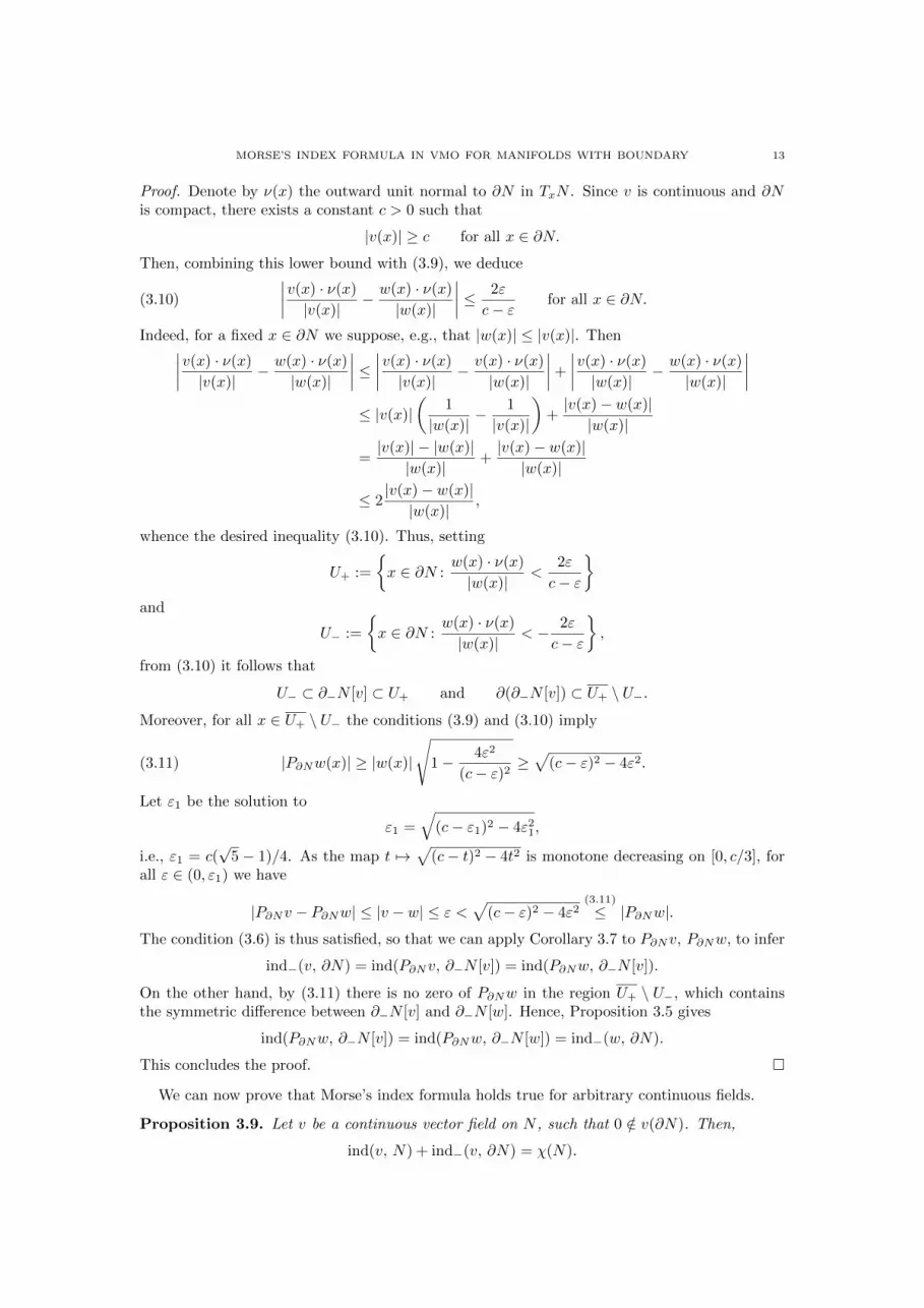
Proof. Denote by ν(x) the outward unit normal to ∂N in TxN . Since v is continuous and ∂Nis compact, there exists a constant c > 0 such that

|v(x)| ≥ c for all x ∈ ∂N.

Then, combining this lower bound with (3.9), we deduce

(3.10)

∣∣∣∣v(x) · ν(x)

|v(x)|− w(x) · ν(x)

|w(x)|

∣∣∣∣ ≤ 2ε

c− εfor all x ∈ ∂N.

Indeed, for a fixed x ∈ ∂N we suppose, e.g., that |w(x)| ≤ |v(x)|. Then∣∣∣∣v(x) · ν(x)

|v(x)|− w(x) · ν(x)

|w(x)|

∣∣∣∣ ≤ ∣∣∣∣v(x) · ν(x)

|v(x)|− v(x) · ν(x)

|w(x)|

∣∣∣∣+

∣∣∣∣v(x) · ν(x)

|w(x)|− w(x) · ν(x)

|w(x)|

∣∣∣∣≤ |v(x)|

(1

|w(x)|− 1

|v(x)|

)+|v(x)− w(x)||w(x)|

=|v(x)| − |w(x)||w(x)|

+|v(x)− w(x)||w(x)|

≤ 2|v(x)− w(x)||w(x)|

,

whence the desired inequality (3.10). Thus, setting

U+ :=

x ∈ ∂N :

w(x) · ν(x)

|w(x)|<

2ε

c− ε

and

U− :=

x ∈ ∂N :

w(x) · ν(x)

|w(x)|< − 2ε

c− ε

,

from (3.10) it follows that

U− ⊂ ∂−N [v] ⊂ U+ and ∂(∂−N [v]) ⊂ U+ \ U−.

Moreover, for all x ∈ U+ \ U− the conditions (3.9) and (3.10) imply

(3.11) |P∂Nw(x)| ≥ |w(x)|

√1− 4ε2

(c− ε)2≥√

(c− ε)2 − 4ε2.

Let ε1 be the solution to

ε1 =√

(c− ε1)2 − 4ε21,

i.e., ε1 = c(√

5 − 1)/4. As the map t 7→√

(c− t)2 − 4t2 is monotone decreasing on [0, c/3], forall ε ∈ (0, ε1) we have

|P∂Nv − P∂Nw| ≤ |v − w| ≤ ε <√

(c− ε)2 − 4ε2(3.11)

≤ |P∂Nw|.

The condition (3.6) is thus satisfied, so that we can apply Corollary 3.7 to P∂Nv, P∂Nw, to infer

ind−(v, ∂N) = ind(P∂Nv, ∂−N [v]) = ind(P∂Nw, ∂−N [v]).

On the other hand, by (3.11) there is no zero of P∂Nw in the region U+ \ U−, which containsthe symmetric difference between ∂−N [v] and ∂−N [w]. Hence, Proposition 3.5 gives

ind(P∂Nw, ∂−N [v]) = ind(P∂Nw, ∂−N [w]) = ind−(w, ∂N).

This concludes the proof.

We can now prove that Morse’s index formula holds true for arbitrary continuous fields.

Proposition 3.9. Let v be a continuous vector field on N , such that 0 /∈ v(∂N). Then,

ind(v, N) + ind−(v, ∂N) = χ(N).

14 GIACOMO CANEVARI, ANTONIO SEGATTI, AND MARCO VENERONI

Proof. We show that it is possible to approximate both v and P∂Nv using the same transversefield u. Then, the proposition will follow by applying the classical Morse’s formula to u.

Owning to the continuity of v, we find a number c > 0 and a neighbourhood U of ∂N in Nsuch that

(3.12) |v(x)| ≥ c for all x ∈ U.

Let ε > 0 be a small parameter, to be chosen later. We fix a smooth vector field v on N suchthat

(3.13) ‖v − v‖C (N) ≤ ε.

Then, by Theorem 3.2, we approximate P∂N v with a transverse vector field ξ on ∂N , such thatξ has finitely many zeros on ∂N and

(3.14) ‖P∂N v − ξ‖C (∂N) ≤ ε.

We claim that there exists a continuous vector field w on N , which is smooth on U , satisfies

w =

ξ + v − P∂N v on ∂N

v on N \ U

and

(3.15) ‖v − w‖C (N) ≤ Cε,

for some constant C depending only on N . (Remark that the prescribed boundary value for wis compatible with the condition (3.15), as it follows from (3.13) and (3.14)). We are giving thedetails of this construction in a moment, but first, we show how to conclude the proof.

By construction, w|∂N is a smooth function satisfying (3.8). For ε small enough, (3.15) andLemma 3.8 entail that

(3.16) ind−(v, ∂N) = ind−(w, ∂N).

Take ε < c/C. Then, (3.12) and (3.15) together imply that w does not vanish on U . Inparticular, w is vacuously transverse on U . Using Theorem 3.2, we modify w out of U to get atransverse vector field u, such that u|U = w|U . As u can be taken arbitrarily close to w in theC -norm, we can assume that (3.4) is satisfied. Hence,

(3.17) ind(v, N) = ind(u, N).

Since u is a transverse field, with finitely many zeros, Morse’s identity applies to u. Then, using(3.16) and (3.17), the proposition follows.

Now, let us explain how to construct the map w. Taking a smaller U if necessary, we canassume that U is a collar of ∂N . This means, U is of the form

U = x ∈ N : dist(x, ∂N) ≤ δ

for some δ > 0, each point x ∈ U has a unique nearest projection σ(x) ∈ ∂N , and the mappingϕ given by

ϕ(x) := (σ(x), |x− σ(x)|) for x ∈ Uis a diffeormorphism U → ∂N × [0, δ]. For each x ∈ U , the differential dϕx is an isomorphism

TxN ' Tσ(x)∂N ⊕ R,

so TxN can be decomposed into a tangential and a normal subspace, with respect to ∂N . Tokeep the notation simple, we assume here that U = ∂N × [0, δ], and ϕ = IdU .

To define w, we interpolate linearly between ξ and the tangential component of v, but weleave the normal component of v unchanged. More precisely, given x = (y, t) ∈ ∂N × [0, δ] we

MORSE’S INDEX FORMULA IN VMO FOR MANIFOLDS WITH BOUNDARY 15

define

w(x) :=

(1− t

δ

)ξ(y) +

t

δP∂N v(x) + v(x)− P∂N v(x)

=

(1− t

δ

)(ξ(y)− P∂N v(x)

)+ v(x)

whereas we setw(x) := v(x) for x ∈ N \ U.

Then w is of class C 1 on U , continuous on N , satisfies w = ξ + v − P∂N v on ∂N . Moreover, forx = (y, t) ∈ U we have

|v(x)− w(x)| ≤(

1− t

δ

) ∣∣ξ(y)− P∂N v(x)∣∣

≤(

1− t

δ

)(∣∣ξ(y)− P∂N v(y, 0)∣∣+∣∣P∂N v(y, 0)− P∂N v(y, t)

∣∣)(3.14)

≤(

1− t

δ

)ε+ t

(1− t

δ

)LipU (P∂N v)

(3.14)

≤ ε+ δC.

By choosing δ small, and combining this inequality with (3.13), we deduce (3.15).

4. The index in the VMO setting

We have now all the necessary tools to define and study the index of a VMO field, which isthe aim of this section. From now on, X will be taken to be the topological double of N , as inSection 2. Moreover, throughout this section we consider a function g ∈ VMO(∂N) such that

(4.1) g(x) ∈ TxN and c1 ≤ |g(x)| ≤ c2 for Hn−1-a.e. x ∈ ∂Nfor some constants c1, c2 > 0. Let v be a VMO vector field with trace g, that is,

(4.2) v ∈ VMOg(N), v(x) ∈ TxN for a.e. x ∈ N.By definition of VMOg(N), the function u given by

u :=

v on N

G on X \N,

where G is the extension of g defined in (2.3), is in VMO(X). Denote the local averages of uand g by

uε(x) :=

BXε (x)

u(y) dσ(y), for x ∈ X.

and

gε(x) :=

B∂Nε (x)

g(y) dHn−1(y), for x ∈ ∂N.

Consider the functions

(4.3) uε := PXuε and gε := PXgε,

defined on X and ∂N , respectively, which are continuous and tangent to X. As we willprove in the following Lemma 4.1, Lemma 4.2, and Lemma 4.5, the quantities ind(uε, N) andind−(gε, ∂N) are well-defined and constant with respect to ε, for ε small enough.

Definition 4.1. Given g ∈ VMO(∂N) and v which satisfy (4.1)–(4.2), we define the index andthe inward boundary index of v by

ind(v, N) := ind(uε, N) and ind−(v, ∂N) := ind−(gε, ∂N),

where ε is fixed arbitrarily in (0, ε0) and ε0 is given by Lemma 4.5.

16 GIACOMO CANEVARI, ANTONIO SEGATTI, AND MARCO VENERONI

Once we have checked that the index, in the sense of Definition 4.1, is well-defined, Theo-rem 1.4 will follow straightforwardly from Proposition 3.9. However, before directing our atten-tion to the main theorem, there are some facts which need to be checked.

The next two lemmas compare the behaviour of gε and uε|∂N .

Lemma 4.1. For every δ > 0, there exists ε0 ∈ (0, r0) so that, for all ε ∈ (0, ε0) and allx ∈ ∂N , we have

c1 − δ ≤ |gε(x)| ≤ c2 + δ.

Lemma 4.2. It holds that

limε→0

supx∈∂N

|uε(x)− gε(x)| = 0.

Combining Lemmas 4.1 and 4.2, we deduce that there exist constants ε0,c > 0 such that

|uε(x)| ≥ c, |gε(x)| ≥ c for all ε ∈ (0, ε0) and all x ∈ ∂N.

In particular,

0 /∈ uε(∂N) and 0 /∈ gε(∂N)

so ind(uε, N) and ind−(gε, ∂N) are well-defined, according to Definition 3.2 and Definition 3.3,for all ε ∈ (0, ε0).

Before proving Lemmas 4.1 and 4.2, we need a useful property.

Lemma 4.3. It holds that

limε→0

supx∈X|uε(x)− uε(x)| = lim

ε→0supx∈∂N

|gε(x)− gε(x)| = 0.

Proof. We present the proof for uε only, as the same argument applies to gε as well. Considera finite atlas A = Uαα∈A for X and, for each α ∈ A, let να1 , . . . , ν

αd−n be a smooth moving

frame for the normal bundle of X, defined on Uα (i.e., (ναi (y))1≤i≤d−n is an orthonormal base

for TyX⊥, for all y ∈ Uα). Set

(4.4) CN := maxα∈A

1≤i≤d−n

‖Dναi ‖L∞(Uα)< +∞.

For all α ∈ A and x ∈ Uα, we write

(4.5) uε(x)− uε(x) =

d−n∑i=1

(uε(x) · ναi (x)) ναi (x)

and, since u(y) · ναi (y) = 0 for a.e. y ∈ Uα, we have

uε(x) · ναi (x) =

Bε(x)

u(y) · (ναi (x)− ναi (y)) dσ(y).

Taking into account (4.4), we infer

|uε(x) · ναi (x)| ≤ CN Bε(x)

|u(y)| |x− y|dσ(y).

To bound the right-side of this inequality, we exploit the injection BMO(X) → Lp(X), whichholds true for all 1 ≤ p < +∞, and the Holder inequality. For a fixed p, we obtain

(4.6) |uε(x) · ναi (x)| ≤ CNσ(Bε(x))−1 ‖x− y‖Lp(Bε(x)) ‖u‖Lp′(X) ≤ CN,n,pε1+n/p−n ‖u‖Lp′(X) ,

for some constant CN,n,p depending only on CN , n and p. Whenever p′ < +∞, the Lp′ norm ofu can be bounded using only the BMO norm of u and

fflXu (with the help of [4, Lemmas A.1

and B.3]). Thus, choosing p = p(n) > 1 so small that 1 + n/p− n > 0, from (4.5) and (4.6) weconclude the proof.

MORSE’S INDEX FORMULA IN VMO FOR MANIFOLDS WITH BOUNDARY 17

Proof of Lemma 4.1. Setting

Sx := v ∈ TxN : c1 ≤ |v| ≤ c2we have, for all x ∈ ∂N ,

(4.7) dist(gε(x), Sx) ≤ Bε(x)

|gε(x)− g(y)| dσ(y) +

Bε(x)

dist(g(y), Sx) dσ(y).

The first term in the right-hand side tends to zero as ε→ 0, uniformly in x, due to Lemma 2.1.On the other hand, it holds

(4.8) supx, y∈∂N

dist(x, y)≤ε

supv∈Sy

dist(v, Sx) −→ 0 as ε→ 0,

since N is compact and smooth up to the boundary. Formula (4.8) can be easily proved, e.g.,by contradiction: Assume that (4.8) does not hold. Then, we find a number η > 0, a sequence(εk)k∈N of positive numbers s.t. εk 0, two sequences (xk)k∈N, (yk)k∈N in N and one (vk)k∈Nin Rd, which satisfy

vk ∈ Syk , dist(xk, yk) ≤ εk, dist(vk, Sxk) ≥ η.By compactness of N , up to subsequences we can assume that

xk → x ∈ N, yk → y ∈ N, vk → v ∈ Rd,where c1 ≤ |v| ≤ c2. Let νi, ν2, . . . , νd−n be a moving frame for the normal bundle of N , definedon a neighbourhood of y. Passing to the limit in the condition

vk · νi(yk) = 0 for all i

we find that v ∈ TyN , hence v ∈ Sy. But y = x, because dist(xk, yk) ≤ εk → 0. Thus, wehave found v ∈ Sx so that dist(v, Sxk) ≥ η/2 > 0. On the other hand, if ϕ : U ⊂ N → Rn is acoordinate chart near x then

wk := dϕ−1ϕ(xk) (dϕxv) , wk := minmax|wk| , c1, c2wk|wk|

are well-defined for k 1 and wk ∈ Sxk , wk → v. This leads to a contradiction.Thus, we can take advantage of (4.1) and (4.8) to estimate the second term in the right-hand

side of (4.7). We deduce that

supx∈∂N

dist(gε(x), Sx) −→ 0 as ε→ 0

and, invoking Lemma 4.3, we conclude the proof.

Proof of Lemma 4.2. In view of Lemma 4.3, proving that

limε→0

supx∈∂N

|uε(x)− gε(x)| = 0

is enough to conclude. In addition, it holds

(4.9) |uε(x)− gε(x)| ≤∣∣uε(x)−Gε(x)

∣∣+∣∣Gε(x)− gε(x)

∣∣ ,so we can study each term in the right-hand side and prove that they converge to zero as ε→ 0.

Let us focus on the first term. We remark that uε −Gε = (u−G)ε and that

u−G =

v −G on N

0 on X \N.

Thus, for all x ∈ ∂N we have (recall that (u−G)(y) = 0 for almost any y ∈ X \N .)

σ(BXε (x) \N

)σ (BXε (x))

∣∣∣(u−G)ε(x)∣∣∣ ≤ 1

σ (BXε (x))

ˆBXε (x)\N

∣∣∣(u−G)(y)− (u−G)ε(x)∣∣∣ dσ(y)

≤ BXε (x)

∣∣∣(u−G)(y)− (u−G)ε(x)∣∣∣ dσ(y),

18 GIACOMO CANEVARI, ANTONIO SEGATTI, AND MARCO VENERONI

where σ is the Riemannian measure on X. Now, assume for a while that there exist two numbersα, ε0 > 0 such that

(4.10)σ(BXε (x) \N

)σ (BXε (x))

≥ α

for all x ∈ ∂N and all ε ∈ (0, ε0). Therefore, when ε < ε0 we deduce

supx∈∂N

∣∣∣(u−G)ε(x)∣∣∣ ≤ α−1 sup

x∈∂N

BXε (x)

∣∣∣(u−G)(y)− (u−G)ε(x)∣∣∣ dσ(y)

and, since u−G ∈ VMO(X), the right-hand side tends to 0 as ε→ 0, by Lemma 2.1. To conclude,we have to prove the validity of (4.10). To this end we assume without loss of generality that N isa smooth, bounded domain inX = Rn. For a fixed x0 ∈ ∂N , we can locally write ∂N as the graphof a smooth function ϕ : Br0(0) ⊆ Rn−1 → R. Then, letting Lx0

(x) := ϕ(x0) + dϕ(x0)(x − x0)be the linear approximation of ϕ, considering the region between the graphs of ϕ and Lx0

wededuce ∣∣∣∣|N ∩Bnε (x0)| − 1

2|Bnε (x0)|

∣∣∣∣ ≤ ˆBn−1ε (x0)

|ϕ(x)− Lx0(x)| dx.

By the Taylor-Lagrange formula, we have |ϕ(x)− Lx0(x)| ≤ M |x− x0|2, for a suitable costantM controlling the hessian of ϕ. Thus∣∣∣∣|N ∩Bnε (x0)| − 1

2|Bnε (x0)|

∣∣∣∣ ≤Mωnεn+2 ,

where ωn := Hn−1(Sn−1) = n |Bn1 (0)|, and

(4.11)

∣∣∣∣ |N ∩Bnε (x0)||Bnε (x0)|

− 1

2

∣∣∣∣ ≤ nMε2 .

The constant M depends on ϕ, which is defined just locally, in a neighbourhood of x0. Never-theless, owning to the compactness of ∂N , one needs to consider a finite number of functionsϕ only, and hence it is possible to choose a constant M which satisfies (4.11) for all x0 ∈ N .Therefore, (4.10) follows.

Now, we have to deal with the second term in (4.9). We can assume, without loss of generality,that X = Rn and

N = Rn+ := (x1, x2, . . . , xn) ∈ Rn : x1 ≥ 0 .We can always reduce to this case by composing with local coordinates, with the help of apartition of the unity argument. For the sake of simplicity, denote the variable in Rn by x =(t, y), where t ∈ R and y ∈ Rn−1.

Call αn the volume of the unit ball of Rn. Using Fubini’s theorem and the definition (2.3) ofG, for x0 = (0, y0) and ε small enough (so that χ(t, y) ≡ 1, for |t| ≤ ε) we compute

Gε(x0) =1

αnεn

ˆ ε

−ε

(ˆBn−1(y0,

√ε2−t2)

G(t, y) dy

)dt

=αn−1αnεn

ˆ ε

−ε

(ε2 − t2

)n−12

( Bn−1(y0,

√ε2−t2)

g(y) dy

)dt

=αn−1αnεn

ˆ ε

−ε

(ε2 − t2

)n−12 g√ε2−t2(y0) dt

=αn−1αnεn

ˆ 1

−1

(ε2 − (εs)2

)n−12 g√

ε2−(εs)2(y0)ε ds

=αn−1αn

ˆ 1

−1

(1− s2

)n−12 gε

√1−s2(y0) ds.

MORSE’S INDEX FORMULA IN VMO FOR MANIFOLDS WITH BOUNDARY 19

On the other hand, Fubini’s theorem also implies that

αn = αn−1

ˆ 1

−1

(1− t2

)n−12 dt,

thus

(4.12)∣∣Gε(x0)− gε(x0)

∣∣ ≤ αn−1αn

ˆ 1

−1

(1− t2

)n−12∣∣gε√1−t2(y0)− gε(y0)

∣∣ dt.

For all −1 < t < 1, since Bn−1(y0, ε√

1− t2) ⊂ Bn−1(y0,√

1− t2) we infer that∣∣gε√1−t2(y0)− gε(y0)∣∣ ≤

Bn−1(y0, ε√1−t2)

|g(y)− gε(y0)| dy

≤(1− t2

) 1−n2

Bn−1(y0, ε)

|g(y)− gε(y0)| dy

and, injecting this information into (4.12), we deduce∣∣Gε(x0)− gε(x0)∣∣ ≤ 2αn−1

αn

Bn−1(y0, ε)

|g(y)− gε(y0)| dy.

Hence, applying once again Lemma 2.1, we conclude that the second term in the right-hand sideof (4.9) converges to zero as ε→ 0, uniformly in x ∈ ∂N .

Remark 4.4. Setting

ind−(g, ∂N) := ind−(uε, ∂N)

gives another possibility to define the inward boundary index of g, just as natural as our Def-inition 4.1. However, thanks to Lemma 4.2 and to the stability of the inward boundary index(Lemma 3.8), we deduce that the two definitions agree.

Lemma 4.5. There exists ε0 ∈ (0, r0) so that the functions

ε 7→ ind(uε, N), ε 7→ ind−(gε, ∂N)

are constant on (0, ε0).

Proof. We have already remarked that ind(uε, N) and ind−(gε, ∂N) are well-defined for ε small,as a consequence of Lemmas 4.1 and 4.2. Consider the functions H : N × (0, ε0) → Rd andG : ∂N × (0, ε0)→ Rd given by

H(x, ε) := uε(x) = projTxN uε(x)

and

G(x, ε) := gε(x) = projTxN gε(x).

These maps are well-defined and continuous. Indeed, it follows from the dominated convergencetheorem that (x, ε) 7→ uε(x) and (x, ε) 7→ gε(x) are continuous, whereas the family of projec-tions projTxN depends continuously on x. Applying Corollary 3.7 and Lemma 3.8 to H and Grespectively, we conclude that ind(uε, N) and ind−(gε, ∂N) are constant with respect to ε.

After these preliminary lemmas, the proof of our main result, Theorem 1.4, is straightforward.

Proof of Theorem 1.4. Let v be given and let uε and gε be the continuous approximants of vand of its trace, as defined in (4.3). Let ε0 > 0 be the constant given by Lemma 4.5. Up tochoosing a smaller value of ε0, owing to Lemma 4.1 and Lemma 4.2, for all ε ∈ (0, ε0) and allx ∈ ∂N we have

|uε(x)| ≥ c12, |gε(x)| ≥ c1

2,

|uε(x)− gε(x)| <√

5− 1

8c1.

20 GIACOMO CANEVARI, ANTONIO SEGATTI, AND MARCO VENERONI

Therefore, by Lemma 3.8, for all ε ∈ (0, ε0)

(4.13) ind−(uε, ∂N) = ind−(gε, ∂N).

To conclude, by Definition 4.1 and Proposition 3.9 we obtain

ind(v, N) + ind−(v, ∂N) = ind(uε, N) + ind−(gε, ∂N)

(4.13)= ind(uε, N) + ind−(uε, ∂N) = χ(N),

which proves Theorem 1.4.

We can finally give the proof of Proposition 1.5.

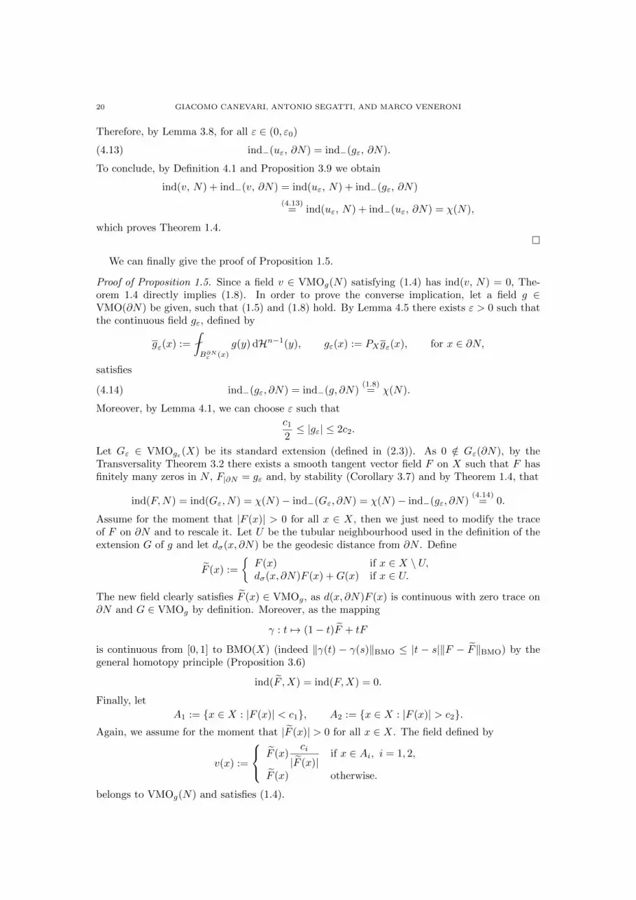
Proof of Proposition 1.5. Since a field v ∈ VMOg(N) satisfying (1.4) has ind(v, N) = 0, The-orem 1.4 directly implies (1.8). In order to prove the converse implication, let a field g ∈VMO(∂N) be given, such that (1.5) and (1.8) hold. By Lemma 4.5 there exists ε > 0 such thatthe continuous field gε, defined by

gε(x) :=

B∂Nε (x)

g(y) dHn−1(y), gε(x) := PXgε(x), for x ∈ ∂N,

satisfies

(4.14) ind−(gε, ∂N) = ind−(g, ∂N)(1.8)= χ(N).

Moreover, by Lemma 4.1, we can choose ε such that

c12≤ |gε| ≤ 2c2.

Let Gε ∈ VMOgε(X) be its standard extension (defined in (2.3)). As 0 /∈ Gε(∂N), by theTransversality Theorem 3.2 there exists a smooth tangent vector field F on X such that F hasfinitely many zeros in N , F|∂N = gε and, by stability (Corollary 3.7) and by Theorem 1.4, that

ind(F,N) = ind(Gε, N) = χ(N)− ind−(Gε, ∂N) = χ(N)− ind−(gε, ∂N)(4.14)

= 0.

Assume for the moment that |F (x)| > 0 for all x ∈ X, then we just need to modify the traceof F on ∂N and to rescale it. Let U be the tubular neighbourhood used in the definition of theextension G of g and let dσ(x, ∂N) be the geodesic distance from ∂N . Define

F (x) :=

F (x) if x ∈ X \ U,dσ(x, ∂N)F (x) +G(x) if x ∈ U.

The new field clearly satisfies F (x) ∈ VMOg, as d(x, ∂N)F (x) is continuous with zero trace on∂N and G ∈ VMOg by definition. Moreover, as the mapping

γ : t 7→ (1− t)F + tF

is continuous from [0, 1] to BMO(X) (indeed ‖γ(t) − γ(s)‖BMO ≤ |t − s|‖F − F‖BMO) by thegeneral homotopy principle (Proposition 3.6)

ind(F ,X) = ind(F,X) = 0.

Finally, let

A1 := x ∈ X : |F (x)| < c1, A2 := x ∈ X : |F (x)| > c2.Again, we assume for the moment that |F (x)| > 0 for all x ∈ X. The field defined by

v(x) :=

F (x)ci

|F (x)|if x ∈ Ai, i = 1, 2,

F (x) otherwise.

belongs to VMOg(N) and satisfies (1.4).

MORSE’S INDEX FORMULA IN VMO FOR MANIFOLDS WITH BOUNDARY 21

To conclude, we note that there is a standard technique to modify a continuous field u suchthat

ind(u,N) = 0, and #x ∈ N : u(x) = 0 < +∞into a continuous field u such that |u| > 0 and u = u on ∂N . We sketch here the idea. First, upto a continuous transformation, we can assume that all the zeros are contained in one coordinateneighbourhood U , with chart φ : U ⊂ N → D ⊂ Rn, so we can reduce to study the vector field incoordinates: let D = B1(0), D1/2 = B1/2(0), assume that u : D → Rn and |u| > 0 in D \D1/2.Then,

0 = ind(u,D) = deg

(u

|u|, ∂D, Sn−1

).

By a classical result (see, e.g., [13]), there exists a harmonic field ψ : D → Sn−1 such thatψ|∂D = u

|u| . Define

ψ(x) :=

ψ(x) if x ∈ D1/2

ψ(x)(2d(x, ∂D) + (1− 2d(x, ∂D)|u(x)|)) if x ∈ D \D1/2,

so that ψ(x) is continuous on D, nowhere zero, and it agrees with u on ∂D. To conclude, thefield

u(x) :=

u if x ∈ N \ Uφ∗ψ if x ∈ U

is continuous and nowhere zero on N . Here φ∗ψ(x) := dφ−1φ(x)ψ(φ(x)) denotes the usual pullback

of ψ via φ.

5. An application: Q-tensor fields and line fields.

In the mathematical modelling of Liquid Crystals two different theories are eminent. In theFrank-Oseen theory the molecules are represented by the unit vector field n which appears inthe energy (1.1). The main drawback of this approach is to neglect the natural head-to-tailsymmetry of the crystals. The theory of Landau-de Gennes takes this symmetry into accountby introducing a tensor-valued field, called Q-tensor, to which is associated a scalar parameters that represents the local average ordered/disordered state of the molecules. In the particular,but physically relevant, case when the order parameter is a positive constant, there is a bijectionbetweenQ-tensors and line fields. The differences between the vector-based and the line field-based theory have been studied in [1], in two- and three-dimensional Euclidean domains. In thisSection we have to aims: firstly we apply the results obtained in Section 4 to line fields on acompact surface, obtaining the VMO-analogue of Poincare-Kneiser Theorem (see Theorem 5.2below); secondly we show how the question of orienting a line field, studied in [1], has generallya negative answer on a compact surface. As it happens for liquid crystals in Euclidean domains,the elastic part of the Landau-de Gennes energy for nematic shells is, at least in some simplifiedsituations, proportional to a Dirichlet type energy. See on this regard [16] and [22]. Therefore,owing to the embedding of Sobolev spaces in VMO spaces, (1.3), Proposition 5.3 establishes arelation between the existence of finite energy Q-tensors with strictly positive order parameterand the topology of the underlying surface, thus extending our application scope from the Frank-Oseen theory to the (constrained) Landau-de Gennes one, for uniaxial nematic shells.

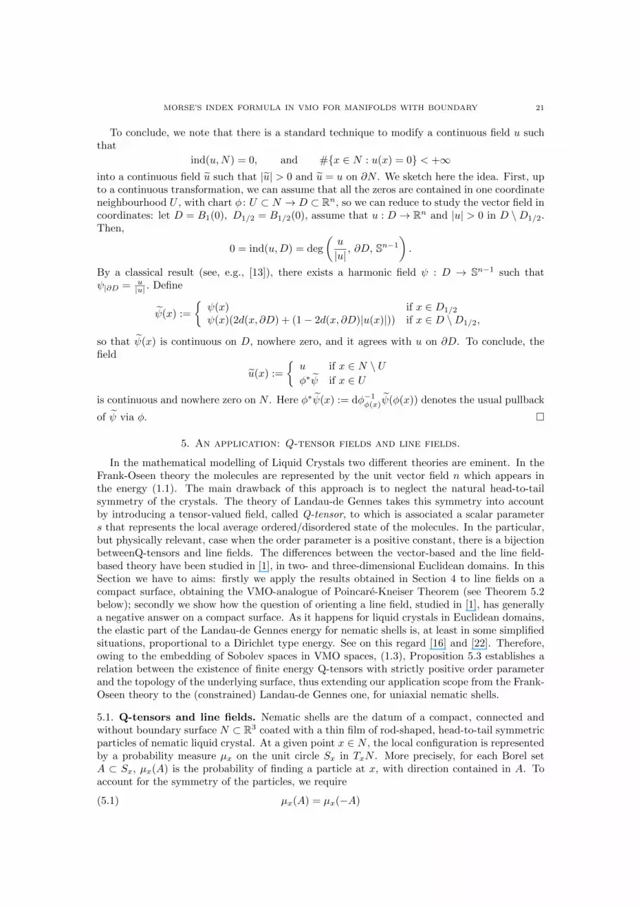
5.1. Q-tensors and line fields. Nematic shells are the datum of a compact, connected andwithout boundary surface N ⊂ R3 coated with a thin film of rod-shaped, head-to-tail symmetricparticles of nematic liquid crystal. At a given point x ∈ N , the local configuration is representedby a probability measure µx on the unit circle Sx in TxN . More precisely, for each Borel setA ⊂ Sx, µx(A) is the probability of finding a particle at x, with direction contained in A. Toaccount for the symmetry of the particles, we require

(5.1) µx(A) = µx(−A)

22 GIACOMO CANEVARI, ANTONIO SEGATTI, AND MARCO VENERONI

for each Borel set A ⊂ Sx. Due to this constraint, the first-order momentum of µx vanishes.Hence, we are naturally led to consider the second-order momentum

(5.2) Q =√

2

ˆSx

(p⊗2 − 1

2Px)

dµx(p),

where (p⊗2)ij := pipj and Px denotes the orthogonal projection on TxN . Note that Q has beensuitably renormalized, so that Q = 0 when µx is the uniform measure, and |Q| = 1 when µx isa Dirac measure concentrated on one direction (see (5.6) and (5.7)). This formula defines a real3× 3 symmetric and traceless matrix called Q-tensor. As we are interested in fields on surfaces,we replaced the usual three-dimensional renormalization term − 1

3Id by − 12Px (see, e.g., [16]).

Once we have fixed an orientation on N , we let γ denote the Gauss map. By definition (5.2),Qγ(x) = 0, which translates the intuitive fact that the probability of finding a particle in thenormal direction of the surface is zero. We call this type of anchoring a degenerate (tangent)anchoring (see [22]).

For any x ∈ N we define the class of “admissible tensors” at x as

(5.3) Qx := Q ∈ S0 : Qγ(x) = 0 ,where S0 is the space of 3× 3 real, symmetric, and traceless matrices, endowed with the scalarproduct Q · P =

∑ij QijPij . It is clear from the definition that Qx is a linear subspace of S0

of dimension 2 (this can be easily checked, e.g., by proving that the map S0 → R3 given byQ 7→ Qγ(x) is surjective). Moreover, Qx varies smoothly with x.

Lemma 5.1. The setQ :=

∐x∈N

Qx,

equipped with the natural projection (x, Q) 7→ x, is a smooth vector bundle on N .

Proof. Consider a smooth orthonormal frame (n, m, γ) defined on a coordinate neighbourhoodof N , where (n, m) is a basis for the tangent bundle of N . With straightforward computations,one can see that the matrices

Xij := ninj −mimj , Yij := nimj +minj ,

Eij := γiγj −1

3δij , Fij := niγj + γinj , Gij := miγj + γimj

define an orthogonal frame for S0. Moreover, (X(x), Y (x)) is a basis for Qx, at each point x (see[14] for a use of this basis with a particular choice for (n,m, γ)). The lemma follows easily.

We can now analyze the special structure of the matrices in Qx. Fix Q ∈ Qx, from (5.3)it follows that γ(x) is an eigenvector of Q, corresponding to the zero eigenvalue. Since Q issymmetric and traceless, there exists an orthonormal basis (n, m) of TxN , whose elements areeigenvectors of Q, and the corresponding eigenvalues are opposite. Thus, denoting by n theeigenvector corresponding to the positive eigenvalue, Q can be written in the form

(5.4) Q =s

2

(n⊗2 −m⊗2

)for some s ≥ 0 (If s = 0, then Q = 0 and any choice of n is allowed). Using the identityn⊗2 + m⊗2 = Px, we conclude that for each Q ∈ Qx there exist a number s ≥ 0 and a unitvector n ∈ TxN such that

(5.5) Q = s

(n⊗2 − 1

2Px).

The number s, called the order parameter, is uniquely determined, and from (5.4) we obtain

(5.6) |Q|2 = Q ·Q =s2

4

(n⊗2 −m⊗2

)·(n⊗2 −m⊗2

)=s2

4

(n⊗2 · n⊗2 +m⊗2 ·m⊗2

)=s2

2.

When Q 6= 0, n is also uniquely determined, up to a sign. Thus, each Q ∈ Qx \ 0 identifies apositive number and a (un oriented) direction in TxN , that is, a line field.

MORSE’S INDEX FORMULA IN VMO FOR MANIFOLDS WITH BOUNDARY 23

A line field on N (also called 1-distribution) is an assignment of a (non zero) tangent direction— but not an orientation — to each point of the submanifold N . More precisely, following [29,Chapter 6] a line field L is a function that assigns to each point x of a manifold N a one-dimensional subspace L(x) ⊂ TxN . Then L is spanned by a vector field locally ; that is, we canchoose a vector field v such that 0 6= v(x) ∈ L(x) for all x in some neighbourhood of x. We saythat L is a smooth (continuous) 1-distribution if the vector field v can be chosen to be smooth(continuous) in a neighbourhood of each point.

Conversely, to a given line ` ⊂ TxN generated by a unit vector ξ ∈ TxN it is possible toassociate the measure µx := 1

2δξ + 12δ−ξ and thus by (5.2) the direction ξ corresponds to

(5.7) Q =√

2

(ξ⊗2 − 1

2P),

which is a unit Q-tensor. The reason for associating to the direction ξ the measure µx =12δξ + 1

2δ−ξ, instead of simply δξ, is to be found in the head-to-tail symmetry of the moleculesexpressed by (5.1). Thus, line fields on N can be identified with sections of the bundle Q, havingmodulus one.

In the following, we relax the condition |Q| = 1, by requiring |Q| to be bounded and uniformlypositive.

5.2. Existence of VMO line fields. In what follows, we assume that N ⊂ R3 is a smooth,compact, connected surface, without boundary. Based on Proposition 1.1 and on the resultsof Section 4, in Proposition 5.3 we prove that the existence of a VMO line field is subject tothe same topological obstruction that holds for continuous vector fields. If we restrict to thecontinuous setting, the following result is classical (see, e.g., [12, Theorem 2.4.6, p. 24])

Theorem 5.2 (Poincare-Kneiser). Let N be a compact, connected submanifold of Rn+1. Thena continuous line field exists if and only if χ(N) = 0.

Definition 5.1. A VMO line field on N is a map Q ∈ VMO(N, S0), such that

(5.8) Q(x) ∈ Qx and c1 ≤ |Q(x)| ≤ c2for some constants c1, c2 > 0 and H2-a.e. x ∈ N .

The condition Q ∈ VMO(N, S0) makes perfectly sense, because S0 ' R5 is a finite-dimensional linear space.

Proposition 5.3. If a VMO line field on N exists, then χ(N) = 0, that is, N has genus 1.

Proof. The proof is based on the arguments of Section 4, with straightforward adaptations. Weapproximate Q with a family of continuos functions, by setting

Qε(x) :=

Bnε (x)

Q(y) dσ(y)

for each x ∈ N and ε ∈ (0, r0). Then, we define

Qε(x) := projQxQε(x) for x ∈ N.

The functions Qε are continuous, since the Qx’s vary smoothly (see Lemma 5.1). Owing to (5.8),and arguing as in Lemma 4.1, it can be proved that

c12≤ |Qε(x)| ≤ 2c2

for all x ∈ N and ε small enough. In view of formula (5.5), each Qε induces a continuous linefield on N . In fact, the continuity of Qε gives the continuity of |Qε|. Consequently, we have thats is a continuous function, thanks to (5.6). On the other hand, the representation formula (5.5)gives that

n⊗2(x) =Q(x)

s(x)+

1

2Px,

24 GIACOMO CANEVARI, ANTONIO SEGATTI, AND MARCO VENERONI

which implies the continuity of n⊗2 thanks to the assumed strict positivity of s and thanks tothe continuity of the projection operator. The tensor n⊗2 is the line field we were looking for.Thus, by Theorem 5.2, it must be χ(N) = 0.

5.3. Orientability of line fields. A typical problem in the study of line fields is to understandin which circumstances a Q-tensor can be described in terms of a vector, that is when, givena tensor field Q with a specified regularity, one can find a unit vector field n with the sameregularity, such that (in three dimensions)

(5.9) Q = s

(n⊗2 − 1

3I)

for some positive constant s. In other words, we are trying to prescribe an orientation for theQ-tensor without creating artificial discontinuities in the vector n. If for a given tensor Q we canfind a vector n for which the representation (5.9) holds, we say that Q is orientable, otherwisenon-orientable. The problem of the orientability of a Q-tensor has been addressed and solvedby Ball and Zarnescu in [1], in the case of two- and three-dimensional Euclidean domains. Theyshowed that the conditions for orienting a given tensor field are of topological as well as ofanalytical nature. Precisely, they require a Sobolev-type regularity, i.e. Q ∈ W 1,p(Ω) withp ≥ 2, together with the condition that the domain Ω be simply connected.

Regarding Q-tensor fields on manifolds (which we assume here to be compact, connected,without boundary), we observe that there exists no two-dimensional surface N and exponentp ≥ 2 such that

Q ∈W 1,p(N) ⇒ Q is orientable.

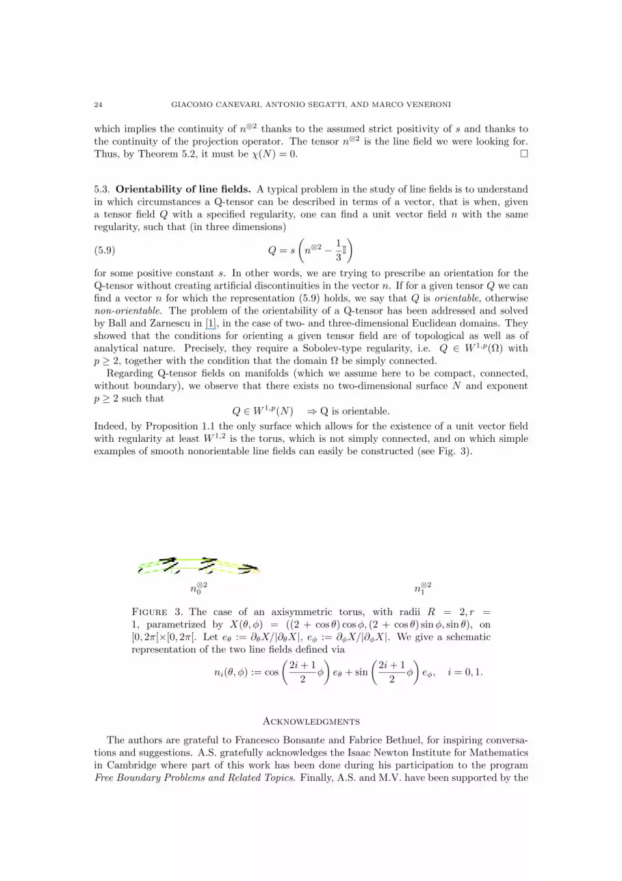
Indeed, by Proposition 1.1 the only surface which allows for the existence of a unit vector fieldwith regularity at least W 1,2 is the torus, which is not simply connected, and on which simpleexamples of smooth nonorientable line fields can easily be constructed (see Fig. 3).

n⊗20 n⊗21

Figure 3. The case of an axisymmetric torus, with radii R = 2, r =1, parametrized by X(θ, φ) = ((2 + cos θ) cosφ, (2 + cos θ) sinφ, sin θ), on[0, 2π[×[0, 2π[. Let eθ := ∂θX/|∂θX|, eφ := ∂φX/|∂φX|. We give a schematicrepresentation of the two line fields defined via

ni(θ, φ) := cos

(2i+ 1

2φ

)eθ + sin

(2i+ 1

2φ

)eφ, i = 0, 1.

Acknowledgments

The authors are grateful to Francesco Bonsante and Fabrice Bethuel, for inspiring conversa-tions and suggestions. A.S. gratefully acknowledges the Isaac Newton Institute for Mathematicsin Cambridge where part of this work has been done during his participation to the programFree Boundary Problems and Related Topics. Finally, A.S. and M.V. have been supported by the

MORSE’S INDEX FORMULA IN VMO FOR MANIFOLDS WITH BOUNDARY 25

Gruppo Nazionale per l’Analisi Matematica, la Probabilita e le loro Applicazioni (GNAMPA)of the Istituto Nazionale di Alta Matematica (INdAM).

References

[1] Ball, J. M., and Zarnescu, A. Orientability and energy minimization in liquid crystal models. Arch.

Ration. Mech. Anal. 202, 2 (2011), 493–535.[2] Bethuel, F. Variational methods for Ginzburg-Landau equations. In Calculus of variations and geometric

evolution problems (Cetraro, 1996), vol. 1713 of Lecture Notes in Math. Springer, Berlin, 1999, pp. 1–43.[3] Bethuel, F., Brezis, H., and Helein, F. Ginzburg-Landau vortices. Progress in Nonlinear Differential

Equations and their Applications, 13. Birkhauser Boston, Inc., Boston, MA, 1994.

[4] Brezis, H., and Nirenberg, L. Degree theory and BMO. I. Compact manifolds without boundaries. SelectaMath. (N.S.) 1, 2 (1995), 197–263.

[5] Brezis, H., and Nirenberg, L. Degree theory and BMO. II. Compact manifolds with boundaries. Selecta

Math. (N.S.) 2, 3 (1996), 309–368. With an appendix by the authors and Petru Mironescu.[6] Brocker, T., and Janich, K. Introduction to differential topology. Cambridge University Press, Cambridge,

1982. Translated from the German by C. B. Thomas and M. J. Thomas.

[7] do Carmo, M. P. Riemannian geometry. Mathematics: Theory & Applications. Birkhauser Boston Inc.,Boston, MA, 1992. Translated from the second Portuguese edition by Francis Flaherty.

[8] Gottlieb, D. H. Vector fields and classical theorems of topology. Rend. Sem. Mat. Fis. Milano 60 (1990),

193–203 (1993).[9] Gottlieb, D. H., and Samaranayake, G. The index of discontinuous vector fields. New York J. Math. 1

(1994/95), 130–148, electronic.[10] Guillemin, V., and Pollack, A. Differential topology. Prentice-Hall Inc., Englewood Cliffs, N.J., 1974.

[11] Hatcher, A. Algebraic topology. Cambridge University Press, Cambridge, 2002.

[12] Hector, G., and Hirsch, U. Introduction to the geometry of foliations. Part A, second ed., vol. 1 of Aspectsof Mathematics. Friedr. Vieweg & Sohn, Braunschweig, 1986. Foliations on compact surfaces, fundamentals

for arbitrary codimension, and holonomy.

[13] Helein, F., and Wood, J. C. Harmonic maps. In Handbook of global analysis. Elsevier Sci. B. V., Amster-dam, 2008, pp. 417–491, 1213.

[14] Ignat, R., Nguyen, L., Slastikov, V., and Zarnescu, A. Stability of the melting hedgehog in the landau-

de gennes theory of nematic liquid crystals. arXiv:1404.1729 (2014).[15] John, F., and Nirenberg, L. On functions of bounded mean oscillation. Comm. Pure Appl. Math. 14

(1961), 415–426.

[16] Kralj, S., Rosso, R., and Virga, E. G. Curvature control of valence on nematic shells. Soft Matter 7(2011), 670–683.

[17] Lloyd, N. G. Degree Theory. Cambridge University Press, Cambridge, 1978. Cambridge Tracts in Mathe-matics, No. 73.

[18] Lubensky, T. C., and Prost, J. Orientational order and vesicle shape. J. Phys. II France 2, 3 (1992),

371–382.[19] Milnor, J. W. Topology from the differentiable viewpoint. Based on notes by David W. Weaver. The Uni-

versity Press of Virginia, Charlottesville, Va., 1965.

[20] Morse, M. Singular points of vector fields under general boundary conditions. Amer. J. Math. 51, 2 (1929),165–178.

[21] Napoli, G., and Vergori, L. Extrinsic curvature effects on nematic shells. Phys. Rev. Lett. 108, 20 (2012),

207803.[22] Napoli, G., and Vergori, L. Surface free energies for nematic shells. Phys. Rev. E 85, 6 (2012), 061701.

[23] Nelson, D. R. Toward a tetravalent chemistry of colloids. Nano Lett. 2, 10 (2002), 1125–1129.[24] Pugh, C. C. A generalized Poincare index formula. Topology 7 (1968), 217–226.[25] Samelson, H. Note on vector fields in manifolds. Proc. Amer. Math. Soc. 36 (1972), 272–274.

[26] Sarason, D. Functions of vanishing mean oscillation. Trans. Amer. Math. Soc. 207 (1975), 391–405.[27] Segatti, A., Snarski, M., and Veneroni, M. Analysis of a variational model for nematic shells. Preprint

Isaac Newton Institute for Mathematical Sciences, Cambridge, NI14037–FRB (2014).

[28] Segatti, A., Snarski, M., and Veneroni, M. Equilibrium configurations of nematic liquid crystals on atorus. Phys. Rev. E 90, 1 (2014), 012501.

[29] Spivak, M. A comprehensive introduction to differential geometry. Vol. I, second ed. Publish or Perish, Inc.,

Wilmington, Del., 1979.[30] Straley, J. Liquid crystals in two dimensions. Phys. Rev. A 4, 2 (1971), 675–681.

[31] Thom, R. Quelques proprietes globales des varietes differentiables. Comment. Math. Helv. 28 (1954), 17–86.

[32] Thom, R. Un lemme sur les applications differentiables. Bol. Soc. Mat. Mexicana (2) 1 (1956), 59–71.

26 GIACOMO CANEVARI, ANTONIO SEGATTI, AND MARCO VENERONI

Sorbonne Universites, UPMC — Universite Paris 06, UMR 7598, Laboratoire Jacques-Louis Lions,

F-75005, Paris, France

E-mail address, G. Canevari: canevari@ann.jussieu.fr

Dipartimento di Matematica “F. Casorati”, Universita di Pavia, Pavia, ItalyE-mail address, A. Segatti: antonio.segatti@unipv.it

E-mail address, M. Veneroni: marco.veneroni@unipv.it