Embed Size (px)
Citation preview

MORTGAGE-BACK SECURITIES
WITH THE
HEATH-JARROW-MORTON MODEL
JIMMY DOYLEMONTE CARLO FOR FINANCIAL MATHEMATICS
1
2 JIMMY DOYLE MONTE CARLO FOR FINANCIAL MATHEMATICS
Executive Summary
To value any fixed income security one needs to evaluate the discounted expected cashflows according to an arbitrage free interest rate model. In the case of mortgage-backedsecurities the future cash flows are uncertain due to mortgage holder exercising of theirprepayment options. This paper considers prepayments which result from interest ratedependent complete refinancing of mortgages in a pool. The rate of refinancing is modeledusing the Heath-Jarrow-Morton Model. The model is implemented in C++ and tested toensure it is behaving correcting. Using this model interest rates used to discount the cashflows are generated. The interest rates are then used to generate refinance rates. Usingthe rates to discount the cash flows and pricing of the MBS. Monte Carlo simulations areapplied to generate 1000 interest rate paths for 1000 different prices and then take averageof them for the actual price. These simulation was used to price Mortgage pass strips: IOand PO strips for a class of 1 year monthly mortgages that had initial principal of 100mortgage rate of .05. The IO came to a price of 2.29537 and the PO was priced at 94.8292.
Background
Mortgage-Backed Securities (MBS) are created by the securitization of mortgages, whichcan be traded in the secondary market. They are created when a financial institutiondecides to sell part of its residual mortgage portfolio to investors. The mortgages soldare put into a pool and investors acquire a stake in the pool by buying units, MBSs.In the secondary market, an investor owns a percentage of the pool is entitled to thesame percentage of principal and interest cash flows received from the mortgages in thepool. They are generally protected from defaults by a government-related agency makesthem appear to be like regular fixed income securities by the government. However, thedifference is that the mortgages have prepayment privileges. Prepayment privileges can bequite valuable to the mortgage holders, giving the holders have an American-style optionto put the mortgage back to the lender at its face value.
Prepayments occur for many reasons: refinancing for lower rates, selling the asset, etc..Prepayments change the methods of valuing of MBSs. A prepayment model describesthe expected prepayments on the underlying pool of mortgages at time t in terms of theyield curve at time t and other relevant variables. For a single mortgages’s prepayments,these models are not useful. The law of large numbers comes into affect due the similarmortgages loans are combined in the same pool and allows for more accurate analysis.There is a tendency for prepayments to be more likely when interest rates are low thanwhen they are high, therefore investors require a higher rate of interest on an MBS thanother fixed-income securities to compensate for the written prepayment options. (Hull)
Methods for Modeling Term Structures. MBSs can be valued using a variety ofMethods, most of them have some sort of use for Monte Carlo simulations. Heath-Jarrow-Morton Method (HJM) and LIBOR Market Method (LMM) of popular methods, and themethods discussed in this paper, used to to simulate the behaviors of the interest ratesmonth by month throughout the life of an MBS. Each month, the expected prepayments
MORTGAGE-BACK SECURITIES WITH THE HEATH-JARROW-MORTON MODEL 3
are calculated from the current yield curve and the history of yield curve movements.These prepayments determine the expected cash flows to the holder of the MBS and thecash flows are discounted to time zero to obtain a sample value for the MBS. An estimateof the value of the MBS is the average of the sample values over many simulation trails.
HJM and LMM are short rate models that more not as easy to implement, but can ensurethat most nonstandard interest rate derivatives are priced consistently with actively tradedinstruments. These models allow the the drift and standard deviation parameters for shortrate models functions of time. They fit term structure and volatility observed in the markettoday.
HJM models the evolution of the term structure through the dynamics of the forwardrate curve. Forward rates are believed to most primitive description of the term structuredue to bond prices and yields reflect averages of forward rates across maturities. Theinstantaneous, continuously compounded forward rates can be considered mathematicalidealizations since they are not directly observable in the marketplace.
Market models are used to describe an approach to interest rate modeling based onobservable market rate, which departs from instantaneous rates. The LMM uses the Lon-don InterBank Offer Rates to express its rates. LIBOR is the most important benchmarkinterest rates, calculated daily for different maturities, and are based on simple interestmake them a great candidate for a market model. (Hull)
Types of MBS. The three majors types of MBS: pass-through securities (PSS), collater-alized mortgages obligations (CMO), and Mortgage Backed Bond (MBB).
PSS ”pass through” promised payments of principal and interest on on mortgages thatare created by financial institutions to secondary market participants holding interests inthe pools. Passthrough securities are created when mortgages are pooled together and par-ticipation certificates in the pool are sold. Typically the mortgages backing a Passthroughsecurity have the same loan type and are similar enough with respect to maturity andloan interest rate to permit cash flow to be projected as if the pool was a single mortgageloan. A pool may consist of many or only a few mortgages. The cash flows are made up ofmonthly mortgage payments. The payments are ade up of interest, scheduled principals,and any prepayment. The pass through cash flows are lower than the actually mortgagepayments due to certain fees, and is taken into account in the passthrough coupon rate.The price of a pass-through MBS is the present value of the projected cash flows discountedat the current yield required by the market, given the specific interest rate and prepaymentrisk of the security in question.
CMOs are mortgage backed bonds issued in multiple classes or branches. They wereintroduced to to broaden the MBS investor base in the 1980s. They allowed more investorsto become active in the MBS market. Financial Institutions could participate in the mar-ket more efficiently by buying short-term mortgage securities to march their short-termliabilities. An investor in a mortgage pass-through security is exposed to prepayment risk.Redirecting how the cash flows of pass-through securities are paid to different bond classesCMOs provide a different exposure to prepayment risk. The basic principle is that redi-recting cash flows (interest and principal) to different bond classes helps different forms of
4 JIMMY DOYLE MONTE CARLO FOR FINANCIAL MATHEMATICS
prepayment risk. It is never possible to eliminate prepayment risk. In order to developrealistic expectation about the performance of CMO bond, an investor must first evaluatethe underlying collateral, since its performance will determine the timing and size of thecash flows reallocated by the CMO structure. Striped CMOs are created by altering thedistribution of principal and interest from a distribution of pass-through security to anunequal distribution The most common type of striped mortgage-backed security is one inwhich all the interest is allocated to IO class and the entire principal is allowed to the POclass .
MBBs are bonds collateralized by a pool of assets. These differ from PSSs and CMOsin major ways. MBBs remain on the balance sheet, therefore not removing the mortgagesfrom a firms balance sheet. The other is that is the cash flows are on the mortgages backingthe bonds do not have have to be directly connected to interest and principal payments onthe MBB. They are mainly used to reduced risk. (Cornet)
Valuing Mortgage-Backed Securities. Projecting a MBS’s cash flows is a necessarytask to value it. . The difficult is that the cash flows are unknown because of prepayment.Assumptions about the prepayments made over the life of the underlying mortgage pool.Two conventions have been used as a benchmark for prepayment rates-conditional pre-payment rate and the public securities association benchmark. Conditional PrepaymentRate (CPR) assumes that some fraction of the remaining principal in a pool of mortgagesis prepaid each month for the remaining term of the mortgage. CPR is based on thecharacteristic of the underlying mortgage pool. The Public Securities Association (PSA)prepayment benchmark is expressed as a monthly series of CPRs. The PSA benchmarkassumes that prepayment rates are low for newly originated mortgages and then will speedup as the mortgages become seasoned.
A prepayment model is a statistical model that is used to forecast prepayments. Itbegins by modeling the statistical relationship among the factors that are expected to affectprepayment. The factors that affect prepayment behavior are: (1) prevailing mortgagerate, (2) characteristics of the underlying mortgage pool, (3) seasonal factors and (4)General economic factors. The single most important factor affecting prepayment becauseof refinancing is the current level of mortgage rates relative to the borrowers contract rate.The more the contract rate exceeds the prevailing mortgage rate the greater the incentiveto refinance the mortgage loan. For refinance to make economic sense the interest savingmust be greater than the cost associated with refinancing the mortgage. These cost includelegal expenses, origination fees, title insurance and the value of the time associated withobtaining the mortgage loan. Historical patterns of prepayment and economic theoriessuggest that, it is not only the level of mortgage rates that affects prepayment behavior,but also the path that mortgage rates take to get to the current level. If the mortgagerate follows a particular path, those who can benefit from refinancing will more than likelytake advantage of this opportunity when the mortgage rate. Anytime interest rates droppeople who can refinance will likely do it. When interest rates keep on dropping, thenthose who can benefit by taken advantage of the refinancing opportunity will have done soalready when rates declined in previous periods. This prepayment behavior is referred to as
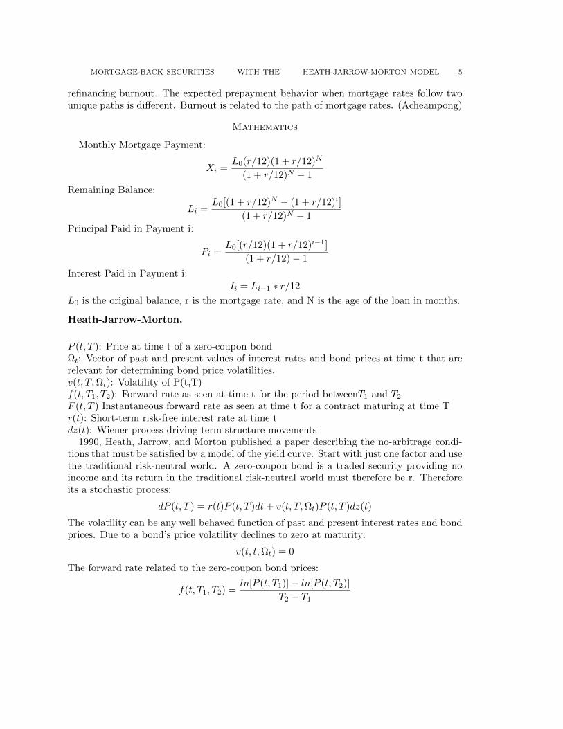
MORTGAGE-BACK SECURITIES WITH THE HEATH-JARROW-MORTON MODEL 5
refinancing burnout. The expected prepayment behavior when mortgage rates follow twounique paths is different. Burnout is related to the path of mortgage rates. (Acheampong)
Mathematics
Monthly Mortgage Payment:
Xi =L0(r/12)(1 + r/12)N
(1 + r/12)N − 1
Remaining Balance:
Li =L0[(1 + r/12)N − (1 + r/12)i]
(1 + r/12)N − 1
Principal Paid in Payment i:
Pi =L0[(r/12)(1 + r/12)i−1]
(1 + r/12)− 1
Interest Paid in Payment i:Ii = Li−1 ∗ r/12
L0 is the original balance, r is the mortgage rate, and N is the age of the loan in months.
Heath-Jarrow-Morton.
P (t, T ): Price at time t of a zero-coupon bondΩt: Vector of past and present values of interest rates and bond prices at time t that arerelevant for determining bond price volatilities.v(t, T,Ωt): Volatility of P(t,T)f(t, T1, T2): Forward rate as seen at time t for the period betweenT1 and T2
F (t, T ) Instantaneous forward rate as seen at time t for a contract maturing at time Tr(t): Short-term risk-free interest rate at time tdz(t): Wiener process driving term structure movements
1990, Heath, Jarrow, and Morton published a paper describing the no-arbitrage condi-tions that must be satisfied by a model of the yield curve. Start with just one factor and usethe traditional risk-neutral world. A zero-coupon bond is a traded security providing noincome and its return in the traditional risk-neutral world must therefore be r. Thereforeits a stochastic process:
dP (t, T ) = r(t)P (t, T )dt+ v(t, T,Ωt)P (t, T )dz(t)
The volatility can be any well behaved function of past and present interest rates and bondprices. Due to a bond’s price volatility declines to zero at maturity:
v(t, t,Ωt) = 0
The forward rate related to the zero-coupon bond prices:
f(t, T1, T2) =ln[P (t, T1)]− ln[P (t, T2)]
T2 − T1
6 JIMMY DOYLE MONTE CARLO FOR FINANCIAL MATHEMATICS
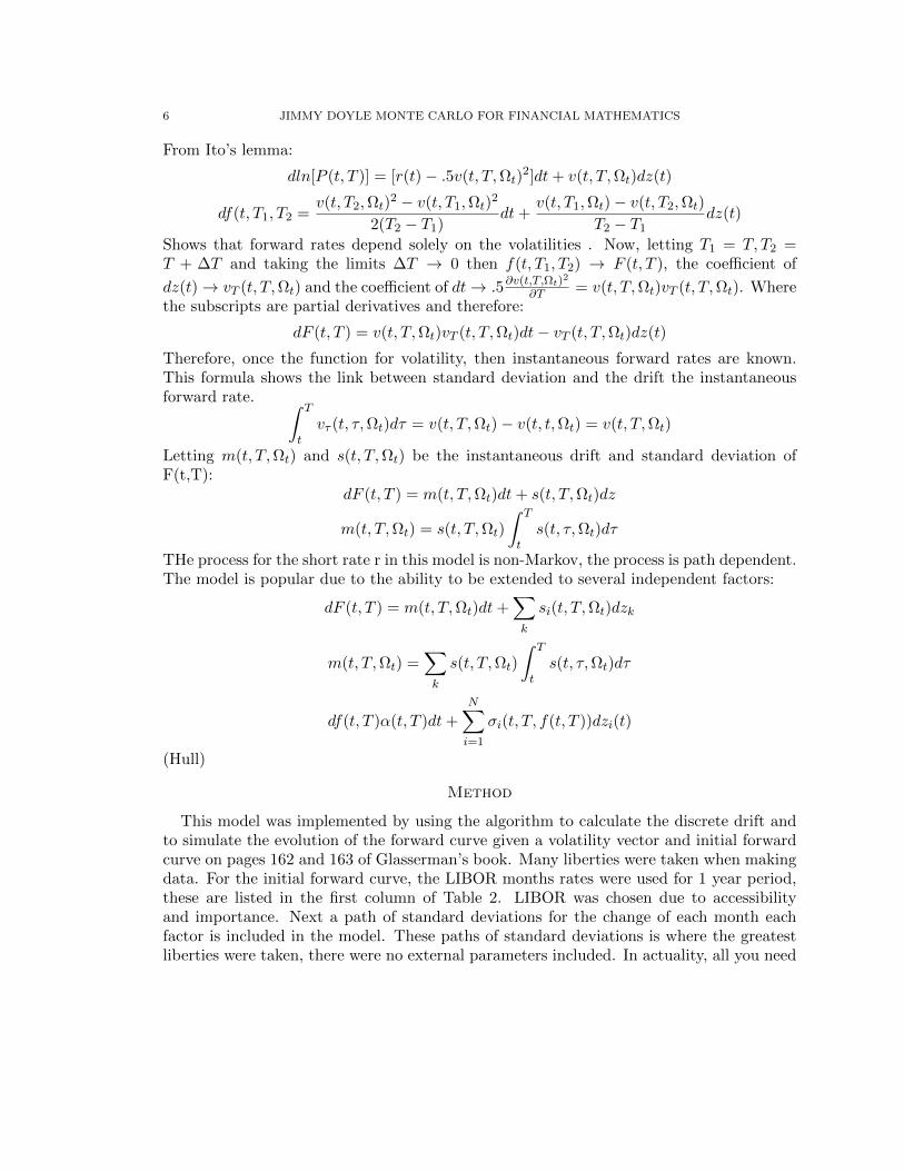
From Ito’s lemma:
dln[P (t, T )] = [r(t)− .5v(t, T,Ωt)2]dt+ v(t, T,Ωt)dz(t)
df(t, T1, T2 =v(t, T2,Ωt)
2 − v(t, T1,Ωt)2
2(T2 − T1)dt+
v(t, T1,Ωt)− v(t, T2,Ωt)
T2 − T1dz(t)
Shows that forward rates depend solely on the volatilities . Now, letting T1 = T, T2 =T + ∆T and taking the limits ∆T → 0 then f(t, T1, T2) → F (t, T ), the coefficient of
dz(t)→ vT (t, T,Ωt) and the coefficient of dt→ .5∂v(t,T,Ωt)2
∂T = v(t, T,Ωt)vT (t, T,Ωt). Wherethe subscripts are partial derivatives and therefore:
dF (t, T ) = v(t, T,Ωt)vT (t, T,Ωt)dt− vT (t, T,Ωt)dz(t)
Therefore, once the function for volatility, then instantaneous forward rates are known.This formula shows the link between standard deviation and the drift the instantaneousforward rate. ∫ T
tvτ (t, τ,Ωt)dτ = v(t, T,Ωt)− v(t, t,Ωt) = v(t, T,Ωt)
Letting m(t, T,Ωt) and s(t, T,Ωt) be the instantaneous drift and standard deviation ofF(t,T):
dF (t, T ) = m(t, T,Ωt)dt+ s(t, T,Ωt)dz
m(t, T,Ωt) = s(t, T,Ωt)
∫ T
ts(t, τ,Ωt)dτ
THe process for the short rate r in this model is non-Markov, the process is path dependent.The model is popular due to the ability to be extended to several independent factors:
dF (t, T ) = m(t, T,Ωt)dt+∑k
si(t, T,Ωt)dzk
m(t, T,Ωt) =∑k
s(t, T,Ωt)
∫ T
ts(t, τ,Ωt)dτ
df(t, T )α(t, T )dt+N∑i=1
σi(t, T, f(t, T ))dzi(t)
(Hull)
Method
This model was implemented by using the algorithm to calculate the discrete drift andto simulate the evolution of the forward curve given a volatility vector and initial forwardcurve on pages 162 and 163 of Glasserman’s book. Many liberties were taken when makingdata. For the initial forward curve, the LIBOR months rates were used for 1 year period,these are listed in the first column of Table 2. LIBOR was chosen due to accessibilityand importance. Next a path of standard deviations for the change of each month eachfactor is included in the model. These paths of standard deviations is where the greatestliberties were taken, there were no external parameters included. In actuality, all you need
MORTGAGE-BACK SECURITIES WITH THE HEATH-JARROW-MORTON MODEL 7
from the parameters are their discrete standard deviations paths. 12 different paths weregenerated using simple methods to keep them realistic but different. The discrete driftwas then computed using the algorithm and the discrete volatilities. These allowed thesimulating the transition from t to ti. Beasley Springer Method was used to generate therandom normal variables needed for Wiener Processes. (Glasserman)
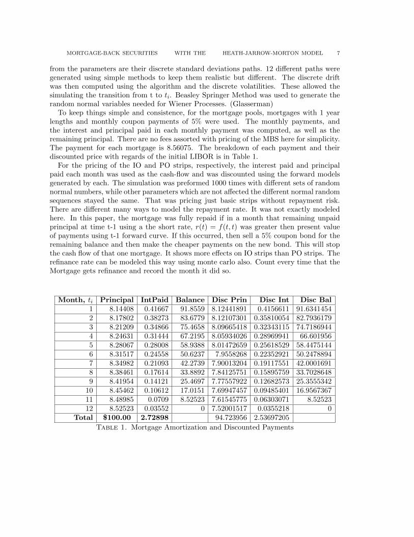
To keep things simple and consistence, for the mortgage pools, mortgages with 1 yearlengths and monthly coupon payments of 5% were used. The monthly payments, andthe interest and principal paid in each monthly payment was computed, as well as theremaining principal. There are no fees assorted with pricing of the MBS here for simplicity.The payment for each mortgage is 8.56075. The breakdown of each payment and theirdiscounted price with regards of the initial LIBOR is in Table 1.
For the pricing of the IO and PO strips, respectively, the interest paid and principalpaid each month was used as the cash-flow and was discounted using the forward modelsgenerated by each. The simulation was preformed 1000 times with different sets of randomnormal numbers, while other parameters which are not affected the different normal randomsequences stayed the same. That was pricing just basic strips without repayment risk.There are different many ways to model the repayment rate. It was not exactly modeledhere. In this paper, the mortgage was fully repaid if in a month that remaining unpaidprincipal at time t-1 using a the short rate, r(t) = f(t, t) was greater then present valueof payments using t-1 forward curve. If this occurred, then sell a 5% coupon bond for theremaining balance and then make the cheaper payments on the new bond. This will stopthe cash flow of that one mortgage. It shows more effects on IO strips than PO strips. Therefinance rate can be modeled this way using monte carlo also. Count every time that theMortgage gets refinance and record the month it did so.
Month, ti Principal IntPaid Balance Disc Prin Disc Int Disc Bal1 8.14408 0.41667 91.8559 8.12441891 0.4156611 91.63414542 8.17802 0.38273 83.6779 8.12107301 0.35810054 82.79361793 8.21209 0.34866 75.4658 8.09665418 0.32343115 74.71869444 8.24631 0.31444 67.2195 8.05934026 0.28969941 66.6019565 8.28067 0.28008 58.9388 8.01472659 0.25618529 58.44751446 8.31517 0.24558 50.6237 7.9558268 0.22352921 50.24788947 8.34982 0.21093 42.2739 7.90013204 0.19117551 42.00016918 8.38461 0.17614 33.8892 7.84125751 0.15895759 33.70286489 8.41954 0.14121 25.4697 7.77557922 0.12682573 25.3555342
10 8.45462 0.10612 17.0151 7.69947457 0.09485401 16.956736711 8.48985 0.0709 8.52523 7.61545775 0.06303071 8.5252312 8.52523 0.03552 0 7.52001517 0.0355218 0
Total $100.00 2.72898 94.723956 2.53697205
Table 1. Mortgage Amortization and Discounted Payments
8 JIMMY DOYLE MONTE CARLO FOR FINANCIAL MATHEMATICS
Results and Conclusions
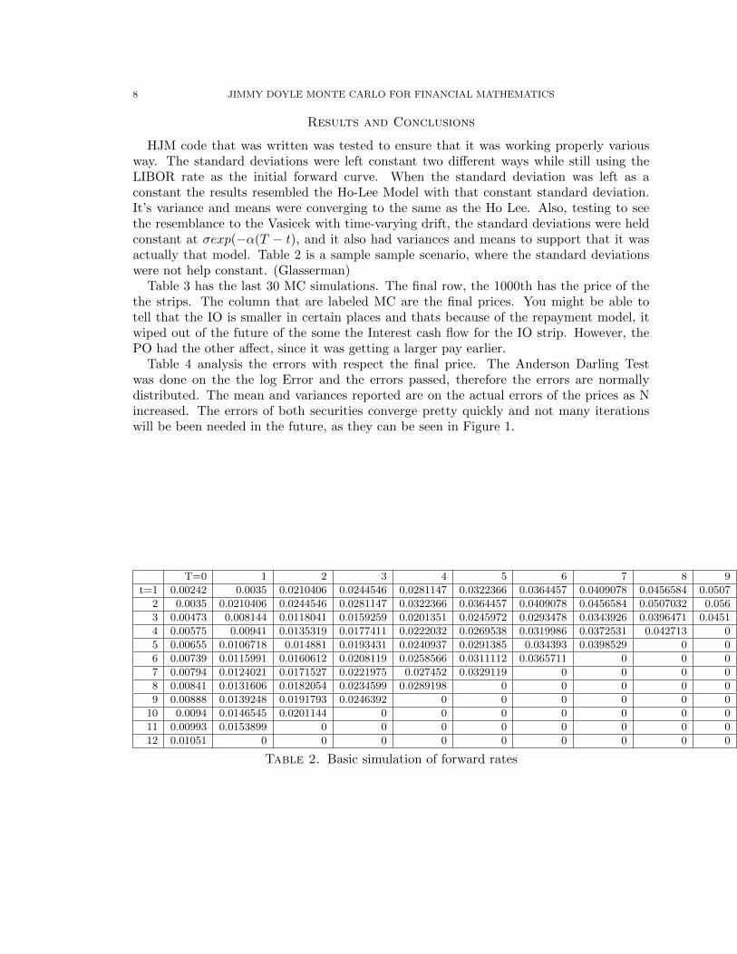
HJM code that was written was tested to ensure that it was working properly variousway. The standard deviations were left constant two different ways while still using theLIBOR rate as the initial forward curve. When the standard deviation was left as aconstant the results resembled the Ho-Lee Model with that constant standard deviation.It’s variance and means were converging to the same as the Ho Lee. Also, testing to seethe resemblance to the Vasicek with time-varying drift, the standard deviations were heldconstant at σexp(−α(T − t), and it also had variances and means to support that it wasactually that model. Table 2 is a sample sample scenario, where the standard deviationswere not help constant. (Glasserman)
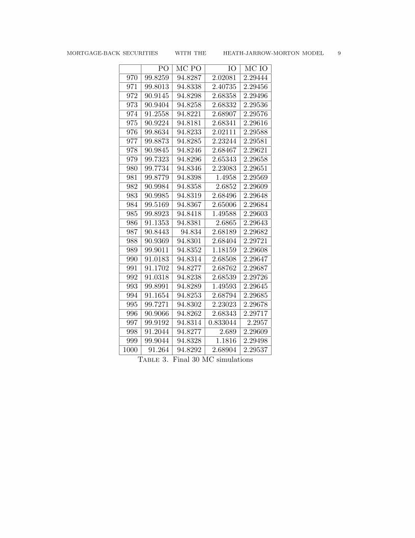
Table 3 has the last 30 MC simulations. The final row, the 1000th has the price of thethe strips. The column that are labeled MC are the final prices. You might be able totell that the IO is smaller in certain places and thats because of the repayment model, itwiped out of the future of the some the Interest cash flow for the IO strip. However, thePO had the other affect, since it was getting a larger pay earlier.
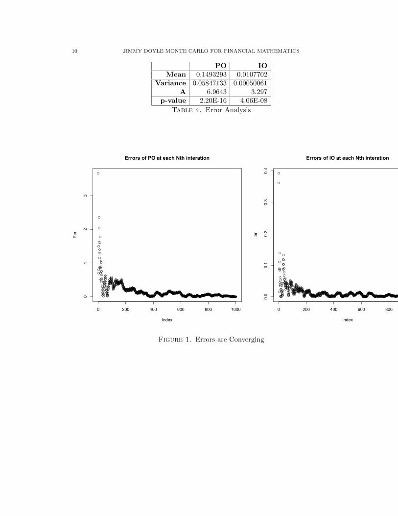
Table 4 analysis the errors with respect the final price. The Anderson Darling Testwas done on the the log Error and the errors passed, therefore the errors are normallydistributed. The mean and variances reported are on the actual errors of the prices as Nincreased. The errors of both securities converge pretty quickly and not many iterationswill be been needed in the future, as they can be seen in Figure 1.
T=0 1 2 3 4 5 6 7 8 9
t=1 0.00242 0.0035 0.0210406 0.0244546 0.0281147 0.0322366 0.0364457 0.0409078 0.0456584 0.0507
2 0.0035 0.0210406 0.0244546 0.0281147 0.0322366 0.0364457 0.0409078 0.0456584 0.0507032 0.056
3 0.00473 0.008144 0.0118041 0.0159259 0.0201351 0.0245972 0.0293478 0.0343926 0.0396471 0.0451
4 0.00575 0.00941 0.0135319 0.0177411 0.0222032 0.0269538 0.0319986 0.0372531 0.042713 0
5 0.00655 0.0106718 0.014881 0.0193431 0.0240937 0.0291385 0.034393 0.0398529 0 0
6 0.00739 0.0115991 0.0160612 0.0208119 0.0258566 0.0311112 0.0365711 0 0 0
7 0.00794 0.0124021 0.0171527 0.0221975 0.027452 0.0329119 0 0 0 0
8 0.00841 0.0131606 0.0182054 0.0234599 0.0289198 0 0 0 0 0
9 0.00888 0.0139248 0.0191793 0.0246392 0 0 0 0 0 0
10 0.0094 0.0146545 0.0201144 0 0 0 0 0 0 0
11 0.00993 0.0153899 0 0 0 0 0 0 0 0
12 0.01051 0 0 0 0 0 0 0 0 0
Table 2. Basic simulation of forward rates
MORTGAGE-BACK SECURITIES WITH THE HEATH-JARROW-MORTON MODEL 9
PO MC PO IO MC IO970 99.8259 94.8287 2.02081 2.29444971 99.8013 94.8338 2.40735 2.29456972 90.9145 94.8298 2.68358 2.29496973 90.9404 94.8258 2.68332 2.29536974 91.2558 94.8221 2.68907 2.29576975 90.9224 94.8181 2.68341 2.29616976 99.8634 94.8233 2.02111 2.29588977 99.8873 94.8285 2.23244 2.29581978 90.9845 94.8246 2.68467 2.29621979 99.7323 94.8296 2.65343 2.29658980 99.7734 94.8346 2.23083 2.29651981 99.8779 94.8398 1.4958 2.29569982 90.9984 94.8358 2.6852 2.29609983 90.9985 94.8319 2.68496 2.29648984 99.5169 94.8367 2.65006 2.29684985 99.8923 94.8418 1.49588 2.29603986 91.1353 94.8381 2.6865 2.29643987 90.8443 94.834 2.68189 2.29682988 90.9369 94.8301 2.68404 2.29721989 99.9011 94.8352 1.18159 2.29608990 91.0183 94.8314 2.68508 2.29647991 91.1702 94.8277 2.68762 2.29687992 91.0318 94.8238 2.68539 2.29726993 99.8991 94.8289 1.49593 2.29645994 91.1654 94.8253 2.68794 2.29685995 99.7271 94.8302 2.23023 2.29678996 90.9066 94.8262 2.68343 2.29717997 99.9192 94.8314 0.833044 2.2957998 91.2044 94.8277 2.689 2.29609999 99.9044 94.8328 1.1816 2.29498
1000 91.264 94.8292 2.68904 2.29537
Table 3. Final 30 MC simulations
10 JIMMY DOYLE MONTE CARLO FOR FINANCIAL MATHEMATICS
PO IOMean 0.1493293 0.0107702
Variance 0.05847133 0.00050061A 6.9643 3.297
p-value 2.20E-16 4.06E-08
Table 4. Error Analysis
0 200 400 600 800 1000
01
23
Errors of PO at each Nth interation
Index
Per
0 200 400 600 800 1000
0.0
0.1
0.2
0.3
0.4
Errors of IO at each Nth interation
Index
Ier
Figure 1. Errors are Converging
MORTGAGE-BACK SECURITIES WITH THE HEATH-JARROW-MORTON MODEL 11
References
Acheampong, Osman, Pricing Mortgage-Backed Securities using Prepayment Functionsand Pathwise Monte Carlo Simulation, 2003.
Baxter, M. and A. Rennie, 1996, Financial Calculus: An introduction to derivative pricing,128-177.
Cornett, Marcia and Saunders, Anthony, Chapter 24: Managing Risk with Loan Salesand Securitization in Financial Markets and Institutions, 2007.
Glasserman, Paul, 2004, Monte Carlo Methods in Financial Engineering, 150-165.
Hull, John, 2006, Options, Futures and other Derivatives, 611-695.
London, Justin, 2004 Modeling Derivatives in C++.
Jordan, B. and Miller, T., Chapter 20: Mortgage-Backed Securities in Fundamentals ofInvestments Valuation and Management, 2008.