Motion-Encoded Particle Swarm Optimizationfor Moving Target Search Using UAVs

Manh Duong Phunga,b,∗, Quang Phuc Haa

aSchool of Electrical and Data Engineering, University of Technology Sydney (UTS)15 Broadway, Ultimo NSW 2007, Australia

bVNU University of Engineering and Technology (VNU-UET), Vietnam National University, Hanoi (VNU)144 Xuan Thuy, Cau Giay, Hanoi, Vietnam

Abstract

This paper presents a novel algorithm named the motion-encoded particle swarm optimization (MPSO) for finding amoving target with unmanned aerial vehicles (UAVs). From the Bayesian theory, the search problem can be convertedto the optimization of a cost function that represents the probability of detecting the target. Here, the proposed MPSOis developed to solve that problem by encoding the search trajectory as a series of UAV motion paths evolving over thegeneration of particles in a PSO algorithm. This motion-encoded approach allows for preserving important propertiesof the swarm including the cognitive and social coherence, and thus resulting in better solutions. Results from extensivesimulations with existing methods show that the proposed MPSO improves the detection performance by 24% andtime performance by 4.71 times compared to the original PSO, and moreover, also outperforms other state-of-the-artmetaheuristic optimization algorithms including the artificial bee colony (ABC), ant colony optimization (ACO), geneticalgorithm (GA), differential evolution (DE), and tree-seed algorithm (TSA) in most search scenarios. Experiments havebeen conducted with real UAVs in searching for a dynamic target in different scenarios to demonstrate MPSO meritsin a practical application.

Keywords: Optimal search, Particle swarm optimization, UAVSource code: The implementation of MPSO can be found at https://github.com/duongpm/MPSO

1. Introduction

Unmanned aerial vehicles (UAVs) have been receivingmuch research interest with numerous practical applica-tions, especially in surveillance and rescue due to theircapability of operating in harsh environments with sensor-rich work capacity suitable for different tasks. In searchingfor a lost target using UAVs, there often exists a criti-cal period called “golden time” in which the probabilitythe target being found should be highest [1]. As timeprogresses, that probability rapidly decreases due to theattenuation of initial information and the influence of ex-ternal factors such as weather conditions, terrain featuresand target dynamics. The main objective in searching fora lost target using UAVs therefore includes finding a paththat can maximize the probability of detecting the targetwithin a specific flight time given initial information ontarget position and search conditions [2, 3].

In the literature, the search problem is often formulatedas probabilistic functions so that uncertainties in initialassumptions, search conditions and sensor models can be

∗Corresponding authorEmail addresses: manhduong.phung@uts.edu.au (Manh Duong

Phung), quang.ha@uts.edu.au (Quang Phuc Ha)

adequately incorporated. In [2, 4], a Bayesian approachhas been introduced to derive the objective functions forevaluating the detection probability of UAV flight paths.The initial search map has been modeled as a multivari-ate normal distribution with the mean and variance beingcomputed based on initial information about the targetposition [5, 6]. In [3, 6], the target dynamic is representedby a stochastic Markov process which can then be deter-ministic or not depending on the searching scenarios. Thesensor, on the other hand, is often modeled as either a bi-nary variable with two states, “detected” or “not detected”[5], or as a continuous Gaussian variable [2].

Due to various probabilistic variables involved, the com-plexity of the searching problem varies from the levelof nondeterministic polynomial-time hardness (NP-hard[7]) to nondeterministic exponential-time completeness(NEXP-complete [8]), in which the number of solutionsavailable to search grows exponentially with respect to thesearch dimension and flight time. Consequently, solvingthis problem using classical methods such as differentialcalculus to find the exact solution becomes impractical,and hence, approximated methods are often used. A num-ber of methods have been developed, such as greedy searchwith one-step look ahead [2] and k-step look ahead [3], ant

1

colony optimization (ACO) [5], Bayesian optimization ap-proach (BOA) [4], genetic algorithm (GA) [9, 10], crossentropy optimization (CEO) [11], branch and bound ap-proach [12], limited depth search [13], and gradient de-scend methods [14, 15]. Table 1 compares main propertiesof some algorithms where the “multi-agent” column im-plies the possibility of using multiple UAVs for searchingand “ad hoc heuristic” for the case being specifically desig-nated for the search problem. It is noted that most meth-ods cope with moving targets and use the binary model fordetection sensors. Some approaches ([4, 5, 11, 13]) employmultiple UAVs to speed up the search process, whereasothers use ad hoc heuristic to improve detection probabil-ity.

From the literature, it is recognizable that approaches tooptimal search diverge in assumptions, constraints, targetdynamics and searching mechanisms. Due to its complexnature, optimal search, especially in scenarios with fast-moving targets, remains a challenging problem. Besides,recent advancements in sensor, communication and UAVtechnologies enable the development of new search plat-forms. They pose the need for new methods that shouldnot only robust in search capacity but also possess prop-erties such as computational efficiency, adaptability andoptimality.

For optimization, particle swarm optimization (PSO) isa potential technique with a number of key advantagesthat have been successfully applied in various applications[16, 17, 18, 19, 20]. It is less sensitive to initial conditionsas well as the variation of objective functions and is ableto adapt to many search scenarios via a small number ofparameters including an initial weight factor and two ac-celeration coefficients [21]. It generally can find the globalsolution with a stable convergence rate and shorter com-putation time compared to other stochastic methods [22].More importantly, PSO is simple in implementation withthe capability of being parallelized to run with not onlycomputer clusters or multiple processors but also graphi-cal processing units (GPU) of a single graphical card. Thisallows to significantly reduce the execution time withoutrequiring any change to the system hardware [23].

Motivated from the aforementioned analysis, we will em-ploy the PSO methodology in this study to deal with thesearch problem in complex scenarios for fast moving tar-gets, aiming to improve the search performance in bothdetection probability and execution time. To this end,we propose a new motion-encoded PSO algorithm, tak-ing into account both cognitive and social coherence ofthe swarm. Our contributions include: (i) the formula-tion of an objective function for optimization, incorporat-ing all assumptions and constraints, from the search prob-lem and the probabilistic framework; (ii) the developmentof a new motion-encoded PSO (MPSO) from the idea ofchanging the search space for the swarm to avoid gettingstuck at local maxima; (iii) the demonstration of MPSOimplemented for UAVs in experimental search scenariosto validate its outperformance over other PSO algorithms

obtained from extensive comparison analysis. The resultsshow that MPSO, on one hand, presents superior perfor-mance on various search scenarios while on the other handremains simple for practical implementation.

The rest of this paper is structured as follows. Section 2outlines the steps to formulate the objective function. Sec-tion 3 presents the proposed MPSO and its implementa-tion for solving a complex search problem. Section 4 pro-vides simulation and experimental results. A conclusion isdrawn in Section 5 to close our paper.

2. Problem Formulation

The search problem is formulated by modeling the tar-get, sensor and belief map with details as follows.

2.1. Target Model

In the searching problem, the target is described by anunknown variable x ∈ X representing its location. Be-fore the search starts, a probability distribution function(PDF) is used to model the target location based on theavailable information, e.g., the last known location of thetarget before losing its signal. This PDF could be a normaldistribution centered about the last known location, butalso could be a uniform PDF if nothing is known aboutthe target location. In the searching space, this PDF isrepresented by a grid map called the belief map, b(x0),in which the value in each cell corresponds to the prob-ability of the target being in that cell. The map can becreated by discretizing the searching space S into a gridof Sr × Sc cells and associating a probability to each cell.Assume the target presents in the searching space, we have∑

x0∈S b(x0) = 1.During the searching process, the target may be not

static but navigate in a certain pattern. This pattern canbe modeled by a stochastic process which can be assumedas a Markov process. In the special case of a conditionallydeterministic target, which is considered in this study, thatpattern merely depends on the initial position x0 of thetarget. In that case, the transition function, p(xt|xt−1),representing the probability which the target goes fromcell xt−1 to xt, is known for all cells xt ∈ S. Consequently,the path of the target will be entirely known if its initialposition is known. This assumption is made quite oftenfor the survivor search at sea [24] and also for the searchproblems in general [5].

2.2. Sensor Model

In order to look for and find a target, a sensor is in-stalled on the UAV to carry out an observation zt at eachtime step t. The observations are independent such thatthe occurrence of one observation provides no informationabout the occurrence of the other observation. A detec-tion algorithm is implemented to return a result for eachobservation which is assumed to have only two possible

2

Table 1: Comparison between search methods

Method Work TargetBinarysensor

Multi-agent

Ad hocheuristic

one-step look ahead [2] Static & Dynamic 7 7 3k-step look ahead [3] Dynamic 3 7 3

BOA [4] Dynamic 3 3 7ACO [5] Dynamic 3 3 3GA [10] Static 3 7 7

CEO [11] Dynamic 3 3 7Depth search [13] Static 3 3 3

Gradient descent [14] Static 7 7 7

outputs, the detection of the target, zt = Dt, or no detec-tion, zt = Dt, where Dt represents a “detection” event attime t. Due to imperfectness of the sensor and detectionalgorithm, an observation of the target detected, zt = Dt,still does not ensure the presence of the target at xt. Thisis reflected through the observation likelihood, p(zt|xt),given knowledge of the sensor model. The likelihood of nodetection, given a target location xt, is then computed by:

p(Dt|xt) = 1− p(Dt|xt). (1)

2.3. Belief Map Update

Once the initial distribution, b(x0), is initialized, thebelief map of the target at time t, b(xt), can be estab-lished based on the Bayesian approach and the sequenceof observations, z1:t = {z1, ..., zt}, made by the sensor.This approach is conducted recursively via two phases,prediction and update. In the prediction, the belief mapis propagated over time in accordance with the target mo-tion model. Suppose at time t, the previous belief map,b(xt−1), is available. Then, the predicted belief map iscalculated as:

b(xt) =∑

xt−1∈Sp(xt|xt−1)b(xt−1). (2)

Notice from (2) that the belief map b(xt−1) is in fact theconditional probability of the target being at xt−1 givenobservations up to t − 1, b(xt−1) = p(xt−1|z1:t−1). Whenthe observation zt is available, the update is conductedsimply by multiplying the predicted belief map by the newconditional observation likelihood as follows:

b(xt) = ηtp(zt|xt)b(xt), (3)

where ηt is the normalization factor,

ηt = 1/∑xt∈S

p(zt|xt)b(xt). (4)

ηt scales the probability that the target presents inside thesearching area to one, i.e.,

∑xt∈S b(xt) = 1.

2.4. Searching Objective Function

According to the Bayesian theory, the probability thatthe target does not get detected at time t during an ob-servation, rt = p(Dt|z1:t−1), relies on two factors: (i) thelatest belief map from the prediction phase (2), and (ii)the no detection likelihood (1). Across the whole search-ing area, that probability is given by:

rt =∑xt∈S

p(Dt|xt)b(xt). (5)

Notice that rt is exactly the inverse of the normalizationfactor ηt in (4), rt = 1/ηt, for a “no detection” event,zt = Dt, and thus is smaller than 1. By multiplying the notdetected probability rt over time, the joint probability offailing to detect the target from time 1 to t, Rt = p(D1:t),is then obtained:

Rt =

t∏k=1

rk = Rt−1rt. (6)

Hence, the probability that the target gets detected for thefirst time at time t is computed as:

pt =

t−1∏k=1

rk(1− rt) = Rt−1(1− rt). (7)

Summing pt over t steps gives the probability of detectingthe target in t steps:

Pt =

t∑k=1

pk = Pt−1 + pt. (8)

Pt is thus often referred to as the “cumulative” probabilityto distinguish it with pt. Notice that

Pt = 1−Rt, (9)

and as t grows, the probability of first detection pt be-comes smaller because the chance of detecting the targetin previous steps increases. The cumulative probabilityPt is thus bounded and increases toward one as t goes toinfinity.

3

The objective function for the searching problem cannow be formulated based on (8) given a finite searchtime. Let the search time period be {1, ..., N}, the goalof the searching strategy is to determine a search pathO = (o1, ..., oN ) that could maximize the cumulative prob-ability Pt. As such, the objective function is eventuallyformulated as follows:

J =

N∑t=1

pt. (10)

3. Motion-encoded Particle Swarm Optimization

As the search problem defined in (10) is NP-hard [7, 8],the time required to calculate all possible paths to findthe optimal solution would greatly increase and becomeintractable. Therefore, a heuristic approach like PSO canbe a good option for solving the optimal search problemas in this study.

3.1. Particle Swarm Optimization

PSO is a population-based stochastic technique, in-spired by social behavior of bird flocking, designed forsolving optimization problems [16, 25]. In PSO, a swarmof particles is initially generated with random positionsand velocities. Each particle then moves and evolves in acognitive fashion with other particles to seek the global op-timum. Those movements are driven by its best position,Lk, and the best position of the swarm, Gk. Let xk andvk be the position and velocity of a particle at generationk, respectively. The movement of that particle in the nextgeneration is given by:

vk+1 ← wvk + ϕ1r1(Lk − xk) + ϕ2r2(Gk − xk) (11)

xk+1 ← xk + vk+1, (12)

where w is the inertial weight, ϕ1 is the cognitive coef-ficient, ϕ2 is the social coefficient, and r1, r2 are randomsequences sampled from a uniform probability distributionin the range [0,1]. From (11) and (12), the movement ofa particle is directed by three factors, namely, followingits own way, moving toward its best position, or movingtoward the swarm’s best position. The ratio among thosefactors is determined by the values of w, ϕ1, and ϕ2.

3.2. MPSO for Optimal Search

There have been several modifications and improve-ments from the PSO algorithm, depending on the appli-cation. However, the implementation of PSO for onlinesearching for dynamic targets in a complex environmentremains a challenging task, particularly in a limited timewindow. For the search problem, it is desired to encodethe position of particles in a way that the particles cangradually move toward the global optimum. A common

3 21

876

5

4

7π( 2, )

4

(1,0)

3π(1, )

2

Figure 1: Motion-encoded illustration for a path with threesegments, Uk = ((1, 0), (1, 3π/2), (

√2, 7π/4))

approach is to define a position as a multi-dimensionalvector representing a possible search path:

xk ∼ Ok = (ok,1, ..., ok,N ), (13)

where ok,i corresponds to a node of the search map [26, 27].The drawback of this approach is that it does not cover theadjacent dynamic behavior in path nodes and thus may re-sult in invalid paths during the searching process. DiscretePSO can be used to overcome this problem, but the mo-mentum of particles is not preserved, causing local maxima[28]. Indirect approaches such as the angle-encoded PSO[29] and priority-based encoding PSO [30] can be a goodoption to deal with it and generate better results. Theirmapping functions, however, require the phase angles tobe within the range of [−π/2, π/2] which limits the searchcapacity, especially in a large dimension.

Here, we propose the idea of using UAV motion to en-code the position of particles. Instead of using nodes, weview each search path as a set of UAV motional segments,each corresponds to the movement of UAV from its cur-rent cell to another on the plane of flight. By respectivelydefining the magnitude and direction of the motion at timet as ρt and αt, that motion can be completely describedby a vector ut = (ρt, αt). A search path is then describedby a vector of N motion segments, Uk = (uk,1, ..., uk,N ).Using Uk as the position of each particle, equations forMPSO can be written as:

∆Uk+1 ← wUk + ϕ1r1(Lk − Uk) + ϕ2r2(Gk − Uk) (14)

Uk+1 ← Uk + ∆Uk+1. (15)

Figure 1 illustrates a path with three segments, Uk =((1, 0), (1, 3π/2), (

√2, 7π/4)), where the belief map is

colour-coded with probability values indicated on theright.

During the search, it is also required to map Uk to adirect path Ok so that the cost associated with Uk can be

4

evaluated. As shown in Fig. 1, the mapping process canbe carried out by first constraining the UAV motion to oneof its eight neighbors in each time step. Then, the motionmagnitude ρt can be normalized and the motion angle αt

can be quantized as:

ρ∗t = 1 (16)

α∗t = 45◦bαt/45◦e, (17)

where be represents the operator for rounding to the near-est integer. Node ok,t+1 corresponding to the location ofUAV in the Cartesian space is then given by:

ok,t+1 = ok,t + u∗k,t, (18)

whereu∗k,t = (bcosα∗t e, bsinα∗t e). (19)

From the decoded path Ok, the cost value can be evalu-ated by the objective function (10) and then the local andglobal best can be computed as follows:

Lk =

{Uk if J(Ok) > J(L∗k−1)Lk−1 otherwise

, (20)

Gk = argmaxLk

J(Ok), (21)

where L∗k is the decoded path of Lk. It can be seen fromthe mapping process that (17) discretizes the motion toone of eight possible directions, (19) converts the movingdirection to an increment in Cartesian coordinates, and(18) incorporates the increment to form the next node ofthe path.

Similarly to the interchange between the time domainand frequency domain in signal analysis, the mapping pro-cess of MPSO allows particles to search in the motion spaceinstead of the Cartesian space. This leads to the followingadvantages:

• The motion space maintains the location of nodes con-secutively so that the resultant paths after each gen-eration evolvement are always valid, which is not thecase of the Cartesian space;

• In motion space, the momentum of particles andswarm behaviors including exploration and exploita-tion are preserved so that the search performance ismaintained and the swarm is able to cope with differ-ent target dynamics;

• As the normalization of ρt and quantization of αt in(16) and (17) are only carried out for the purpose ofcost evaluation, their continuous values are still be-ing used for velocity and position updates as in (14)- (15). This property is important to avoid the dis-cretizing effect of PSO so that the search resolution isnot affected.

Finally, it is also noted that MPSO preserves the searchmechanism of PSO via its update equations (14) - (15)so that the advantages of PSO such as stable convergence,independence of initial conditions and implementation fea-sibility can be maintained.

Start

Initialize the belief map and particles with motion-

encoded paths

Compute the cumulative probability via objective function

Decode the paths encoded in particles’ position

Update the velocity and position of particles

Get target dynamics and initial data

Update the local best and global best

Check maximum generation

End

No

Yes

Figure 2: Flowchart of MPSO algorithm

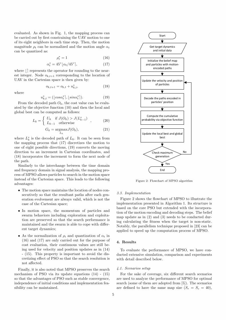
3.3. Implementation

Figure 2 shows the flowchart of MPSO to illustrate theimplementation presented in Algorithm 1. Its structure isbased on the core PSO but extended with the incorpora-tion of the motion encoding and decoding steps. The beliefmap update as in (2) and (3) needs to be conducted dur-ing calculating the fitness when the target is non-static.Notably, the parallelism technique proposed in [23] can beapplied to speed up the computation process of MPSO.

4. Results

To evaluate the performance of MPSO, we have con-ducted extensive simulation, comparison and experimentswith detail described below.

4.1. Scenarios setup

For the sake of coverage, six different search scenariosare used to analyze the performance of MPSO for optimalsearch (some of them are adopted from [5]). The scenariosare defined to have the same map size (Sr = Sc = 40),

5

/* Initialization: */

Get target dynamics and initial data;Create belief map;Set swarm parameters w, ϕ1, ϕ2, swarm size;foreach particle in swarm do

Create random motion-encoded paths Uk;Assign Uk to particle position;Compute fitness value of each particle;Set local best value of each particle to itself;Set velocity of each particle to zero;

endSet global best to the best fit particle;/* Evolutions: */

for k ← 1 to max generation doforeach particle in swarm do

Compute motion velocity ∆Uk+1; /* Eq.14

*/

Compute new position Uk+1; /* Eq.15 */

Decode Uk+1 to Ok+1; /* Eq.19 - 18 */

Update fitness of Ok+1; /* Eq.10 */

Update local best Lk+1; /* Eq.20 */

endUpdate global best Gk+1; /* Eq.21 */

end

Algorithm 1: Pseudo code of MPSO.

but differ in the initial locations of UAV, target motionmodel P (xt|xt−1) and initial belief map b(x0). As shownin Fig.3, the probability map is color-coded with the tar-get dynamics presented by a white arrow and the initiallocation of UAV described by a white circle. The scenariosrepresent different searching situations as follows:

Scenario 1 has two high probability regions locatednext to each other. They are slightly different in locationand value, which may cause difficulty in finding a betterregion to search for the target.

Scenario 2 includes two separated high probability re-gions located opposite to each other over the UAV location.The algorithm has to quickly identify the higher proba-bility region to search and track as the target is movingsouth-west.

Scenario 3 has one small dense region moving rapidlytoward the south-east. It thus tests the algorithm in itsexploration and adaptation capability.

Scenario 4 is similar to Scenario 3 except that the tar-get is moving toward the UAV’s start location. It furtherevaluates the adaptability of the searching algorithm.

Scenario 5 consists of two probability regions locatedoppositely via the start location in which the right regionis slightly higher in probability. As the target is movingnorth, the algorithm needs to identify the correct targetregion.

Scenario 6 is similar to Scenario 5, but the start loca-tion is below the potential regions and the target is movingNorth-East. It thus evaluates the capability of searching

in a diagonal direction.In our evaluations, MPSO is implemented with the pa-

rameters w = 1 at the damping rate of 0.98, ϕ1 = 2.5 andϕ2 = 2.5. The swarm size is chosen to be 1000 particles.The number of iterations is 100 and the size of the searchpath is 20 nodes. Due to the stochastic nature of PSO,the algorithm is executed 10 times to find the average andstandard deviation values for each scenario.

4.2. Search path

Figure 4 shows the search paths of MPSO for each sce-nario together with the cumulative probability values. Inall scenarios, MPSO is able to find the highest probabilityregions and generates relevant paths for the UAV to fly.For scenarios with only one high probability region suchas Scenario 3 and 4, the cumulative probabilities are highbecause the chance of finding the target is not spread toother regions. It is also noted from Fig. 4 that the prob-ability map only reflects the target belief at the last stepwhereas the search path represents the tracking of highprobability regions over time. By comparing them withthose in Fig. 3, we can see that the search paths adapt tothe target dynamics to maximize the detection probability.

4.3. Comparison with other PSO algorithms

We have judged the merit of MPSO over other PSO algo-rithms including a classical PSO, denoted here as PSO forthe comparison purpose, quantum-behaved PSO (QPSO)and angle-encoded PSO (APSO).

PSO is introduced in [16] in which the particles encodea search path as a set of nodes. They then evolve accordingto (11) and (12) to find the optimal solution.

APSO operates in a similar way as PSO. It, however,encodes the position of particles as a set of phase angles sothat each angle represents the direction in which the pathwould emerge [29].

QPSO, on the other hand, assumes particles to havequantum behavior in a bound state. The particles areattracted by a quantum potential well centered on its localattractor and thus have a new stochastic update equationfor their positions [31]. In QPSO, the position of particlesalso encodes a search path that includes a set of nodes.

Table 2 shows the average and standard deviation val-ues of the fitness representing the accumulated detectionprobability obtained by all algorithms after 10 runs. It canbe seen that MPSO introduces the best performance in 5scenarios. APSO is slightly better than MPSO in Scenario3, but its convergence is not stable reflected via a largerstandard deviation value. These results can be furtherverified via the convergence curves shown in Fig. 5. Theyshow that PSO and QPSO present poor performance asthe use of nodes to encode search paths does not maintainparticle momentum resulting in local maxima.

APSO, on the other hand, introduces a comparable per-formance with MPSO. Unlike PSO and QPSO, the use ofangles in APSO allows particles to search in orientation

6

10 20 30 40

x (cell)

10

20

30

40

y (c

ell)

5

10

15

10 -3

10 20 30 40

x (cell)

10

20

30

40

y (c

ell)

5

10

15

10 -3

(a) Scenario 1

10 20 30 40

x (cell)

5

10

15

20

25

30

35

40

y (c

ell)

5

10

15

10 -3

10 20 30 40

x (cell)

5

10

15

20

25

30

35

40

y (c

ell)

5

10

15

10 -3

(b) Scenario 2

10 20 30 40

x (cell)

5

10

15

20

25

30

35

40

y (c

ell)

10

20

30

40

50

60

70

10-3

10 20 30 40

x (cell)

5

10

15

20

25

30

35

40

y (c

ell)

10

20

30

40

50

60

70

10-3

(c) Scenario 3

10 20 30 40

x (cell)

5

10

15

20

25

30

35

40y

(ce

ll)

10

20

30

40

50

60

70

10 -3

10 20 30 40

x (cell)

5

10

15

20

25

30

35

40y

(ce

ll)

10

20

30

40

50

60

70

10 -3

(d) Scenario 4

10 20 30 40

x (cell)

5

10

15

20

25

30

35

40

y (c

ell)

5

10

15

20

10 -3

10 20 30 40

x (cell)

5

10

15

20

25

30

35

40

y (c

ell)

5

10

15

20

10 -3

(e) Scenario 5

10 20 30 40

x (cell)

5

10

15

20

25

30

35

40

y (c

ell)

5

10

15

20

10 -3

10 20 30 40

x (cell)

5

10

15

20

25

30

35

40

y (c

ell)

5

10

15

20

10 -3

(f) Scenario 6

Figure 3: Scenarios used for evaluating the searching algorithms

7

10 20 30 40x (cell)

5

10

15

20

25

30

35

40

y (c

ell)

0

5

10

15

10-3

(a) Scenario 1: Pt = 0.1886

10 20 30 40x (cell)

5

10

15

20

25

30

35

40

y (c

ell)

0

5

10

15

10-3

(b) Scenario 2: Pt = 0.2496

10 20 30 40x (cell)

5

10

15

20

25

30

35

40

y (c

ell)

0

10

20

30

40

50

60

70

10-3

(c) Scenario 3: Pt = 0.64907

10 20 30 40

x (cell)

5

10

15

20

25

30

35

40y

(cel

l)

0

10

20

30

40

50

60

70

10-3

(d) Scenario 4: Pt = 0.5111

10 20 30 40

x (cell)

5

10

15

20

25

30

35

40

y (c

ell)

0

5

10

15

2010-3

(e) Scenario 5: Pt = 0.2226

10 20 30 40x (cell)

5

10

15

20

25

30

35

40

y (c

ell)

0

5

10

15

2010-3

(f) Scenario 6: Pt = 0.1907

Figure 4: Search paths for each scenario generated by MPSO

8

Table 2: Comparison between PSO algorithms on fitness representing the accumulated detection probability

Scenario MPSO PSO QPSO APSO1 0.1876±0.0011 0.1476 ±0.0043 0.1198±0.0037 0.1869±0.00252 0.247±0.0055 0.2019±0.0163 0.2014±0.0046 0.2393±0.01133 0.6554±0.014 0.5403±0.0218 0.5468±0.014 0.6649±0.02874 0.5018±0.0095 0.4082±0.0092 0.4259±0.0164 0.4969±0.01095 0.2213±0.0025 0.1785±0.0067 0.1819±0.0008 0.2199±0.0046 0.1881±0.0112 0.097±0.0239 0.0943±0.0168 0.1735±0.0187

space and thus maintains the swarm properties. Interest-ingly, APSO can be considered as a special case of MPSOwhen the motion magnitude is constrained to 1. Whilethis constraint limits the flexibility of the swarm, it mayimprove the exploration capacity in certain scenarios toyield a good result such as in Scenario 3.

4.4. Comparison with metaheuristic optimization algo-rithms

To further evaluate the performance of MPSO, wehave compared it with state-of-the-art metaheuristic op-timization algorithms including the artificial bee colony(ABC), ant colony optimization (ACO), genetic algorithm(GA), differential evolution (DE), and tree-seed algorithm(TSA).

ABC searches for optimal solutions based on the co-operative behavior of three types of bees: employed bees,onlooker bees and scout bees [32]. Our implementationrepresents each solution as a search path that consists ofa set of motion segments similar to MPSO.

ACO solves optimization problems based on heuristicinformation and a pheromone model of artificial ants, eachmaintains a feasible solution [33]. Our implementation ofACO is based on [5] in which the “ACO-Node+H” ap-proach is used together with the max-min ACO.

GA is a popular metaheuristic optimization that modi-fies a population of individual solutions similar to the pro-cess of natural selection [9]. Our implementation of GA isbased on the “EA-dir” approach in [10] where a path is en-coded as a string of directions subjected to two mutationtechniques including “flip” and “pull”.

DE is an optimization method that finds the optimal so-lution by improving its candidates via simple mathemati-cal formulas from a population of individual solutions [34].In implementing DE for optimal search, we represent eachsolution as a set of motions similar to the representationused in MPSO.

TSA solves the optimization problem by simultaneouslyexploring and exploiting the search space based on thespread of seeds from a tree population. The level andbalance between the exploration and exploitation are con-trolled by predefined parameters including the search ten-dency (ST ) and the number of seeds (NS). Those pa-rameters are chosen as in the original study [35] in ourimplementation, i.e., ST = 0.1 and NS ∈ [0.1, 0.25].

Table 3 presents the fitness values corresponding to theoptimal solutions of MPSO and metaheuristic algorithmsover six scenarios after 10 runs. The values include the av-erage and standard deviation representing the cumulativedetection probability. It can be seen that MPSO outper-forms other metaheuristic algorithms in scenarios 1 to 5with the highest fitness values and small standard devia-tion. TSA is the second best with satisfactory results inmost scenarios, whereas the remaining algorithms are onlygood in one or two scenarios.

Figure 6 further compares the convergence among thealgorithms. While MPSO shows good exploitation capa-bility represented via the high fitness value in most sce-narios, its exploration reflected via the convergence speedis rather slow in some scenarios such as Scenario 3 wherethe high probability region is small and the target is mov-ing away from the UAV. TSA, on the other hand, is goodat exploration but rather limited in exploitation so thatits final fitness values are slightly less than MPSO. ACOperforms well in detecting static and slow-moving targets,but its adaptation to fast-moving targets is limited due tothe nature of ACO incrementally exploring via nodes. DEand ABC have stable performance in most scenarios. GA,on the other hand, is often trapped at local minimums asthe crossover and mutation operators cause many invalidpaths during operation. Besides, the enhanced “flip” and“pull” operators which prioritize horizontal and verticalsearch do not perform well in scenarios requiring diagonalsearch such as Scenario 6.

4.5. Execution time

Apart from the accuracy, we also evaluate the executiontime of all algorithms to roughly estimate their complex-ity. We executed all algorithms under the same conditionsof software and computer hardware. Table 4 shows theaverage execution time together with the standard devi-ation after 10 runs on an Intel Core i7-7600U 2.80 GHzprocessor. It can be seen that MPSO is the fastest in fourscenarios, followed by ABC with two scenarios. DE alsointroduces relatively short execution time due to its sim-plicity in the search mechanism. TSA, on the other hand,is rather slow due to the extra computation required toevaluate the seeds of each tree. ACO is the slowest becauseof a large time spent on calculating heuristic information[5]. Notably, the execution time of APSO is close to MPSOwhich further explains it as a special case of MPSO. PSO

9

0 20 40 60 80 100Number of Iterations

0

0.05

0.1

0.15

0.2

Fitn

ess

Val

ue

MPSOPSOQPSOAPSO

0 20 40 60 80 100Number of Iterations

0

0.05

0.1

0.15

0.2

Fitn

ess

Val

ue

(a) Scenario 1

0 20 40 60 80 100Number of Iterations

0

0.05

0.1

0.15

0.2

0.25

Fitn

ess

Val

ue

MPSOPSOQPSOAPSO

0 20 40 60 80 100Number of Iterations

0

0.05

0.1

0.15

0.2

0.25

Fitn

ess

Val

ue(b) Scenario 2

0 20 40 60 80 100

Number of Iterations

0

0.2

0.4

0.6

0.8

Fitn

ess

Val

ue

MPSOPSOQPSOAPSO

0 20 40 60 80 100

Number of Iterations

0

0.2

0.4

0.6

0.8

Fitn

ess

Val

ue

(c) Scenario 3

0 20 40 60 80 100Number of Iterations

0

0.1

0.2

0.3

0.4

0.5

0.6

Fitn

ess

Val

ue

MPSOPSOQPSOAPSO

0 20 40 60 80 100Number of Iterations

0

0.1

0.2

0.3

0.4

0.5

0.6

Fitn

ess

Val

ue

(d) Scenario 4

0 20 40 60 80 100Number of Iterations

0

0.05

0.1

0.15

0.2

0.25

Fitn

ess

Val

ue

MPSOPSOQPSOAPSO

0 20 40 60 80 100Number of Iterations

0

0.05

0.1

0.15

0.2

0.25

Fitn

ess

Val

ue

(e) Scenario 5

0 20 40 60 80 100Number of Iterations

0

0.05

0.1

0.15

0.2

Fitn

ess

Val

ue

MPSOPSOQPSOAPSO

0 20 40 60 80 100Number of Iterations

0

0.05

0.1

0.15

0.2

Fitn

ess

Val

ue

(f) Scenario 6

Figure 5: Convergence curves of the four PSO algorithms on the six benchmark scenarios

10

0 20 40 60 80 100

Number of Iterations

0

0.05

0.1

0.15

0.2

Fitn

ess

Val

ue

MPSOABCACO

GADETSA

0 20 40 60 80 100

Number of Iterations

0

0.05

0.1

0.15

0.2

Fitn

ess

Val

ue

(a) Scenario 1

0 20 40 60 80 100

Number of Iterations

0

0.05

0.1

0.15

0.2

0.25

Fitn

ess

Val

ue

MPSOABCACO

GADETSA

0 20 40 60 80 100

Number of Iterations

0

0.05

0.1

0.15

0.2

0.25

Fitn

ess

Val

ue(b) Scenario 2

0 20 40 60 80 100

Number of Iterations

0

0.2

0.4

0.6

0.8

Fitn

ess

Val

ue

MPSOABCACO

GADETSA

0 20 40 60 80 100

Number of Iterations

0

0.2

0.4

0.6

0.8

Fitn

ess

Val

ue

(c) Scenario 3

0 20 40 60 80 100

Number of Iterations

0

0.1

0.2

0.3

0.4

0.5

0.6

Fitn

ess

Val

ue

MPSOABCACO

GADETSA

0 20 40 60 80 100

Number of Iterations

0

0.1

0.2

0.3

0.4

0.5

0.6

Fitn

ess

Val

ue

(d) Scenario 4

0 20 40 60 80 100

Number of Iterations

0

0.05

0.1

0.15

0.2

0.25

Fitn

ess

Val

ue

MPSOABCACO

GADETSA

0 20 40 60 80 100

Number of Iterations

0

0.05

0.1

0.15

0.2

0.25

Fitn

ess

Val

ue

(e) Scenario 5

0 20 40 60 80 100

Number of Iterations

0

0.05

0.1

0.15

0.2

Fitn

ess

Val

ue

MPSOABCACO

GADETSA

0 20 40 60 80 100

Number of Iterations

0

0.05

0.1

0.15

0.2

Fitn

ess

Val

ue

(f) Scenario 6

Figure 6: Convergence curves of MPSO and other metaheuristic algorithms on the six benchmark scenarios

11

Table 3: Comparison between MPSO and other metaheuristic algorithms on fitness

Scenario MPSO ABC GA ACO DE TSA1 0.1876±0.0011 0.1691±0.0076 0.1283±0.0001 0.1836±0.0013 0.1818±0.0015 0.1873±0.00062 0.247±0.0055 0.2099±0.0041 0.2151±0.0018 0.2145±0.0049 0.22±0.0045 0.2362±0.00853 0.6554±0.014 0.5872±0.0152 0.5995±0.003 0.6053±0.02 0.5985±0.0166 0.6236±0.01354 0.5018±0.0095 0.4225±0.0017 0.3497±0.0311 0.4866±0.0139 0.4243±0.0252 0.4626±0.02395 0.2213±0.0025 0.2093±0.0071 0.1733±0.0001 0.2208±0.0024 0.2128±0.006 0.2209±0.00056 0.1881±0.0112 0.181±0.0019 0.1255±0.0001 0.15±0.0119 0.1829±0.0139 0.1889±0.0018

and QPSO both require extra execution time due to theinvalid paths generated during operation.

4.6. Validation on UAV platform

To demonstrate the practical use of MPSO, we haveapplied it to real searching scenarios with details as follows.

4.6.1. Experimental setup

The experiment is carried out in the search area of 60m × 60 m located in a park in Sydney. The UAV usedis a 3DR Solo drone with a control architecture developedfor infrastructure inspection [36] that can be controlledvia a ground control station (GCS) software named Mis-sion Planner. The detection sensor is a Hero 4 cameraattached to the drone via a three-axis gimble responsiblefor adjusting and stabilizing the camera. An unmannedground vehicle (UGV) is used as the target. The UGVis equipped with control and communication modules toallow it to track certain trajectories for the sake of exper-imental verification.

In experiments, initial locations of UAV and UGV areobtained via the GPS modules equipped on those vehiclesand used as the input to generate a belief map. The map isfed to MPSO to generate a search path that includes a listof waypoints. Those waypoints are loaded into MissionPlanner to fly the UAV. During the flight, for recordingthe testing results, positions of the vehicles are tracked viaGPS and the video received from the camera is streamedto GCS.

4.6.2. Experimental results

Figure 7a shows the belief map and path generated byMPSO for the scenario in which the UGV started from thecenter of the map at the latitude of -33.875992 and the lon-gitude of 151.19145 and moved in East direction. Figure7b shows the planned and actual flight paths recorded viaMission Planner together with the actual path of UGV. Itcan be seen that the flight path tracks the planned pathwith some inevitably small tracking errors caused by GPSpositioning. Those errors can be compensated for by ex-tending the field of view of the detection camera via theflight attitude. The UAV thus can trace and approach thetarget at the location of (-33.87598,151.19153), as shownin Figure 7b. This can be verified in Fig. 8 that displaysthe target within the vision of the camera.

In another experiment where the UGV moves towardthe starting location of the UAV, the planned pathadapts to it by turning backward as shown in Fig. 7c.Figure 7d presents the actual trajectories of the UAVand UGV. It can be seen that the UAV tracks theplanned path to approach the target at the location of(-33.875938,151.191515) and then can trace it eventually.Those results, together with various successful trials, con-firm the validity and applicability of our proposed algo-rithm.

4.7. Discussion

Through extensive simulation, thorough comparisonand experiments as described above, it can be seen thatMPSO presents better performance than other state-of-the-art heuristic algorithms in most search scenarios andis suitable for practical UAV search operations. The ratio-nale for the success of MPSO lies in the motion-encodedmechanism that prevents the algorithm from generatinginvalid paths during the searching process so that it canavoid the need for re-initialization, and as such, to acceler-ate the convergence. The motion-encoded mechanism alsoallows MPSO to search in the motion space instead of theCartesian space to improve search performance and bet-ter adapt to target dynamics. This advantage is clearlyreflected in the good search result of MPSO for the chal-lenging Scenario 4 where the target moves in the oppo-site direction to the search path that requires the UAVto turn around. Nevertheless, like PSO, MPSO may needto increase the swarm size and number of iterations if thesearch dimension increases [37]. In those scenarios, par-allel implementation is required to effectively reduce thecomputation time, and hence, improve the scalability ofthe proposed algorithm for large-scale systems.

In practical search, the target dynamics may vary de-pending on the applications so that the deterministic as-sumption used in this study may go beyond its validity.In those scenarios, a prediction mechanism using optimalestimators such as the Kalman filter [38] can be employedto provide a prediction of the target trajectory. It is thenused to calculate the cumulative probability used in theobjective function of MPSO.

12

Table 4: Comparison between MPSO and other algorithms on execution time in seconds

Scenario MPSO PSO QPSO APSO ABC GA ACO DE TSA1 43±2 129±6 140±15 50±8 34±1 85±2 144±3 37±3 84±22 26±4 150±7 180±22 34±4 34±5 95±3 157±2 32±6 57±63 30±8 142±4 149±3 39±4 31±4 97±1 150±5 34±2 50±24 20±2 149±7 149±1 32±5 30±3 92±3 133±3 26±3 47±15 29±7 126±4 129±5 46±5 34±4 92±3 150±4 31±3 60±56 48±7 140±3 139±2 61±1 39±3 99±2 146±13 39±3 85±2

5 10 15 20x (cell)

5

10

15

20

y (c

ell)

0

20

40

60

80

100

10-3

(a) Belief map and search path in experimental scenario 1

Target trajectory

Planned path

UAV trajectory

Start

End

(b) Planned and actual flight paths in experimental scenario 1

5 10 15 20x (cell)

5

10

15

20

y (c

ell)

0

20

40

60

80

100

10-3

(c) Belief map and search path in experimental scenario 2

Target trajectory

Planned path

UAV trajectory

Start

End

(d) Planned and actual flight paths in experimental scenario 2

Figure 7: Experimental detection results

13

Drone

Target

Target viewed from drone

Figure 8: The target within the vision of the camera attached onthe drone

5. Conclusion

We have presented a new algorithm, the motion-encodedparticle swarm optimization (MPSO), to solve the prob-lem of optimal search for a moving target using UAVs. Thealgorithm encodes the search path as a series of motionsthat are directly applicable to the search problem whichconstrains the movement of a UAV to its neighbor cells.By changing the search domain from the Cartesian spaceto motion space, the algorithm is able to adapt to differenttarget dynamics. It also preserves key properties of PSOto enhance the search performance and allows to conductcontinuous search in discrete maps. Simulation and ex-perimental results show that the algorithm is effective andpractical enough to deploy for search operations. To beeffective also for large-scale systems, the proposed algo-rithm would need parallel computation to further reduceits execution time. Our future work will focus on evalu-ating MPSO on benchmarking functions and exploring itscapability to solve other complex optimization problems.

References

[1] S. F. Ochoa, R. Santos, Human-centric wireless sensor net-works to improve information availability during urban searchand rescue activities, Information Fusion 22 (2015) 71 – 84.doi:10.1016/j.inffus.2013.05.009.

[2] F. Bourgault, T. Furukawa, H. F. Durrant-Whyte, OptimalSearch for a Lost Target in a Bayesian World, Springer BerlinHeidelberg, Berlin, Heidelberg, 2006, pp. 209–222. doi:10.

1007/10991459_21.[3] M. Raap, S. Meyer-Nieberg, S. Pickl, M. Zsifkovits, Aerial ve-

hicle search-path optimization: A novel method for emergencyoperations, Journal of Optimization Theory and Applications172 (3) (2017) 965–983. doi:10.1007/s10957-016-1014-y.

[4] P. Lanillos, J. Yanez Zuluaga, J. J. Ruz, E. Besada-Portas, Abayesian approach for constrained multi-agent minimum timesearch in uncertain dynamic domains, in: Proceedings of the

15th Annual Conference on Genetic and Evolutionary Compu-tation, GECCO ’13, ACM, New York, NY, USA, 2013, pp. 391–398. doi:10.1145/2463372.2463417.

[5] S. Perez-Carabaza, E. Besada-Portas, J. A. Lopez-Orozco, J. M.de la Cruz, Ant colony optimization for multi-uav minimumtime search in uncertain domains, Applied Soft Computing 62(2018) 789 – 806. doi:10.1016/j.asoc.2017.09.009.

[6] T. Furukawa, F. Bourgault, B. Lavis, H. F. Durrant-Whyte,Recursive bayesian search-and-tracking using coordinated uavsfor lost targets, in: Proceedings 2006 IEEE International Con-ference on Robotics and Automation, 2006. ICRA 2006., 2006,pp. 2521–2526. doi:10.1109/ROBOT.2006.1642081.

[7] K. E. Trummel, J. R. Weisinger, Technical note - the complex-ity of the optimal searcher path problem, Operations Research34 (2) (1986) 324–327. doi:10.1287/opre.34.2.324.

[8] D. S. Bernstein, R. Givan, N. Immerman, S. Zilberstein, Thecomplexity of decentralized control of markov decision pro-cesses, Mathematics of Operations Research 27 (4) (2002) 819–840. doi:10.1287/moor.27.4.819.297.

[9] D. E. Goldberg, Genetic Algorithms in Search, Optimizationand Machine Learning, 1st Edition, Addison-Wesley LongmanPublishing Co., Inc., Boston, MA, USA, 1989.

[10] L. Lin, M. A. Goodrich, UAV intelligent path planning forwilderness search and rescue, in: 2009 IEEE/RSJ InternationalConference on Intelligent Robots and Systems, 2009, pp. 709–714. doi:10.1109/IROS.2009.5354455.

[11] P. Lanillos, E. Besada-Portas, G. Pajares, J. J. Ruz, Mini-mum time search for lost targets using cross entropy optimiza-tion, in: 2012 IEEE/RSJ International Conference on Intelli-gent Robots and Systems, 2012, pp. 602–609. doi:10.1109/

IROS.2012.6385510.[12] J. N. Eagle, J. R. Yee, An optimal branch-and-bound procedure

for the constrained path, moving target search problem, Oper-ations Research 38 (1) (1990) 110–114. doi:10.1287/opre.38.

1.110.[13] A. Sarmiento, R. Murrieta-Cid, S. Hutchinson, An effi-

cient motion strategy to compute expected-time locally op-timal continuous search paths in known environments, Ad-vanced Robotics 23 (12-13) (2009) 1533–1560. doi:10.1163/

016918609X12496339799170.[14] S. K. Gan, S. Sukkarieh, Multi-UAV target search using ex-

plicit decentralized gradient-based negotiation, in: 2011 IEEEInternational Conference on Robotics and Automation, 2011,pp. 751–756. doi:10.1109/ICRA.2011.5979704.

[15] G. Mathews, H. Durrant-Whyte, M. Prokopenko, Asynchronousgradient-based optimisation for team decision making, in: 200746th IEEE Conference on Decision and Control, 2007, pp. 3145–3150. doi:10.1109/CDC.2007.4434301.

[16] J. Kennedy, R. Eberhart, Y. Shi (Eds.), Swarm Intelligence,Morgan Kaufmann, 2001. doi:10.1016/B978-1-55860-595-4.

X5000-1.[17] K. Y. Lee, J. Park, Application of particle swarm optimization

to economic dispatch problem: Advantages and disadvantages,in: 2006 IEEE PES Power Systems Conference and Exposition,2006, pp. 188–192.

[18] V. Mohammadi, S. Ghaemi, H. Kharrati, PSO tuned FLC forfull autopilot control of quadrotor to tackle wind disturbanceusing bond graph approach, Applied Soft Computing 65 (2018)184 – 195. doi:10.1016/j.asoc.2018.01.015.

[19] T. Niknam, M. R. Narimani, M. Jabbari, Dynamic optimalpower flow using hybrid particle swarm optimization and simu-lated annealing, International Transactions on Electrical EnergySystems 23 (7) (2013) 975–1001. doi:10.1002/etep.1633.

[20] T. Niknam, M. R. Narimani, J. Aghaei, R. Azizipanah-Abarghooee, Improved particle swarm optimisation for multi-objective optimal power flow considering the cost, loss, emis-sion and voltage stability index, IET Generation, TransmissionDistribution 6 (6) (2012) 515–527.

[21] R. C. Eberhart, Y. Shi, Comparison between genetic algorithmsand particle swarm optimization, in: V. W. Porto, N. Sara-vanan, D. Waagen, A. E. Eiben (Eds.), Evolutionary Program-

14

ming VII, Springer Berlin Heidelberg, Berlin, Heidelberg, 1998,pp. 611–616.

[22] Zwe-Lee Gaing, Particle swarm optimization to solving the eco-nomic dispatch considering the generator constraints, IEEETransactions on Power Systems 18 (3) (2003) 1187–1195.

[23] M. D. Phung, C. H. Quach, T. H. Dinh, Q. Ha, Enhanced dis-crete particle swarm optimization path planning for UAV vision-based surface inspection, Automation in Construction 81 (2017)25 – 33. doi:10.1016/j.autcon.2017.04.013.

[24] K. Iida, R. Hohzaki, K. Inada, Optimal survivor search for a tar-get with conditionally deterministic motion under reward crite-rion, Journal of the Operations Research Society of Japan 41 (2)(1998) 246–260. doi:10.15807/jorsj.41.246.

[25] M. Kohler, M. M. Vellasco, R. Tanscheit, PSO+: A new par-ticle swarm optimization algorithm for constrained problems,Applied Soft Computing 85 (2019) 105865. doi:10.1016/j.

asoc.2019.105865.[26] V. Roberge, M. Tarbouchi, G. Labonte, Comparison of parallel

genetic algorithm and particle swarm optimization for real-timeuav path planning, IEEE Transactions on Industrial Informatics9 (1) (2013) 132–141. doi:10.1109/TII.2012.2198665.

[27] Y. Zhang, D. wei Gong, J. hua Zhang, Robot path planningin uncertain environment using multi-objective particle swarmoptimization, Neurocomputing 103 (2013) 172 – 185. doi:10.

1016/j.neucom.2012.09.019.[28] M. Clerc, Discrete Particle Swarm Optimization, illustrated

by the Traveling Salesman Problem, Springer Berlin Heidel-berg, Berlin, Heidelberg, 2004, pp. 219–239. doi:10.1007/

978-3-540-39930-8_8.[29] Y. Fu, M. Ding, C. Zhou, Phase angle-encoded and

quantum-behaved particle swarm optimization applied to three-dimensional route planning for UAV, IEEE Transactions on Sys-tems, Man, and Cybernetics - Part A: Systems and Humans42 (2) (2012) 511–526. doi:10.1109/TSMCA.2011.2159586.

[30] A. W. Mohemmed, N. C. Sahoo, T. K. Geok, Solving short-est path problem using particle swarm optimization, AppliedSoft Computing 8 (4) (2008) 1643 – 1653, soft Computing forDynamic Data Mining. doi:10.1016/j.asoc.2008.01.002.

[31] J. Sun, W. Fang, X. Wu, V. Palade, W. Xu, Quantum-behavedparticle swarm optimization: Analysis of individual particlebehavior and parameter selection, Evolutionary Computation20 (3) (2012) 349–393, pMID: 21905841. doi:10.1162/EVCO_a_

00049.[32] D. Karaboga, B. Basturk, On the performance of artificial bee

colony (ABC) algorithm, Applied Soft Computing 8 (1) (2008)687 – 697. doi:10.1016/j.asoc.2007.05.007.

[33] M. Dorigo, T. Stutzle, The Ant Colony Optimization Meta-heuristic: Algorithms, Applications, and Advances, SpringerUS, Boston, MA, 2003, pp. 250–285. doi:10.1007/

0-306-48056-5_9.[34] R. Storn, K. Price, Differential evolution–a simple and efficient

heuristic for global optimization over continuous spaces, Journalof global optimization 11 (4) (1997) 341–359. doi:10.1023/A:

1008202821328.[35] M. S. Kiran, Tsa: Tree-seed algorithm for continuous optimiza-

tion, Expert Systems with Applications 42 (19) (2015) 6686 –6698. doi:10.1016/j.eswa.2015.04.055.

[36] V. T. Hoang, M. D. Phung, T. H. Dinh, Q. P. Ha, System ar-chitecture for real-time surface inspection using multiple UAVs,IEEE Systems Journal (2019) 1–12doi:10.1109/JSYST.2019.2922290.

[37] S. Piccand, M. O’Neill, J. Walker, On the scalability of particleswarm optimisation, in: 2008 IEEE Congress on EvolutionaryComputation (IEEE World Congress on Computational Intelli-gence), 2008, pp. 2505–2512.

[38] H. Musoff, P. Zarchan, Fundamentals of Kalman filtering: apractical approach, American Institute of Aeronautics and As-tronautics, 2009.

15