Moving Gravitational Lenses: imprints on the CMB

arX

iv:a

stro

-ph/

9803

040v

1 4

Mar

199

8A&A manuscript no.(will be inserted by hand later)

Your thesaurus codes are:12(12.03.1,12.03.3, 12.07.1)

ASTRONOMYAND

ASTROPHYSICS

Moving gravitational lenses: imprints on the CMB

N. Aghanim1, S. Prunet1, O. Forni1, and F. R. Bouchet2

1 IAS-CNRS, Universite Paris XI, Batiment 121, F-91405 Orsay Cedex2 IAP-CNRS, 98 bis, Boulevard Arago, F-75014 Paris

Received date / accepted date

Abstract. With the new generation of instruments forCosmic Microwave Background (CMB) observations aim-ing at an accuracy level of a few percent in the measure-ment of the angular power spectrum of the anisotropies,the study of the contributions due to secondary effectshas gained impetus. Furthermore, a reinvestigation of themain secondary effects is crucial in order to predict andquantify their effects on the CMB and the errors that theyinduce in the measurements.

In this paper, we investigate the contribution, to theCMB, of secondary anisotropies induced by the transversemotions of clusters of galaxies. This effect is similar to theKaiser–Stebbins effect. In order to address this problem,we model the gravitational potential well of an individ-ual structure using the Navarro, Frenk & White profile.We generalise the effect of one structure to a populationof objects predicted using the Press-Schechter formalism.We simulate maps of these secondary fluctuations, com-pute the angular power spectrum and derive the averagecontributions for three cosmological models. We then in-vestigate a simple method to separate this new contribu-tion from the primary anisotropies and from the main sec-ondary effect, the Sunyaev-Zel’dovich kinetic effect fromthe lensing clusters.

Key words: Cosmology: cosmic microwave background –gravitational lensing – secondary fluctuations – clusters ofgalaxies

1. Introduction

During the next decade, several experiments are plannedto observe the Cosmic Microwave Background (CMB) andmeasure its temperature fluctuations (Planck surveyor,Map, Boomerang, ...). Their challenge is to measure thesmall scales anisotropies of the CMB (a few arcminutesup to ten degrees scale) with sensitivities better by afactor 10 than the COBE satellite (Smoot et al. 1992).These high sensitivity and resolution measurements will

Send offprint requests to: N. Aghanim

tightly constrain the value of the main cosmological pa-rameters (Kamionkowski et al. 1994). However, the con-straints can only be set if we are able to effectively measurethe primary temperature fluctuations. These fluctuations,present at recombination, give an insight into the earlyuniverse since they are directly related to the initial den-sity perturbations which are the progenitors to the cosmicstructures (galaxies and galaxies clusters) in the presentuniverse; but which are first and foremost the relics of thevery early initial conditions of the universe.Between recombination and the present time, the CMBphotons could have undergone various interactions withthe matter and structures present along their lines of sight.Some of these interactions can induce additional tem-perature fluctuations called, secondary anisotropies be-cause they are generated after the recombination. Alonga line of sight, one measures temperature fluctuationswhich are the superposition of the primary and secondary

anisotropies. As a result, and in the context of the futureCMB experiments, accurate analysis of the data will beneeded in order to account for the foreground contribu-tions due to the secondary fluctuations. Photon–matterinteractions between recombination and the present timeare due to the presence of ionised matter or to variationsof the gravitational potential wells along the lines of sight.

The CMB photons interact with the ionised mattermainly through Compton interactions. In fact, after re-combination the universe could have been re-ionised glob-ally or locally. Global early re-ionisation has been widelystudied (see Dodelson & Jubas 1995 for a recent re-view and references therein). Its main effect is to eithersmooth or wipe out some of the primary anisotropies;but the interactions of the photons with the matter ina fully ionised universe can also give rise to secondaryanisotropies through the Vishniac effect (Vishniac 1987).This second order effect has maximum amplitudes fora very early re-ionisation. The case of a late inhomoge-neous re-ionisation and its imprints on the CMB fluctu-ations has been investigated (Aghanim et al. 1996) andfound to be rather important. In this case, the secondaryanisotropies are due to the bulk motion of ionised cloudswith respect to the CMB frame. When the re-ionisation

http://arXiv.org/abs/astro-ph/9803040v1

2 N. Aghanim et al.: Moving gravitational lenses: imprints on the CMB

is localised in hot ionised intra-cluster media the pho-tons interact with the free electrons. The inverse Comptonscattering between photons and electrons leads to the so-called Sunyaev-Zel’dovich (hereafter SZ) effect (Sunyaev& Zel’dovich1972, 1980). The Compton distortion due tothe motion of the electrons in the gas is called the ther-mal SZ effect. The kinetic SZ effect is a Doppler distor-tion due to the peculiar bulk motion of the cluster withrespect to the Hubble flow. The SZ thermal effect has theunique property of depressing the CMB brightness in theRayleigh-Jeans region and increasing its brightness abovea frequency of about 219 GHz. This frequency dependencemakes it rather easy to observe and separate from the ki-netic SZ effect. In fact, the latter has a black body spec-trum which makes the spectral confusion between kineticSZ and primary fluctuations a serious problem. The SZeffect has been widely studied for individual clusters andfor populations of clusters. For full reviews on the subjectwe refer the reader to two major articles: Rephaeli 1995and Birkinshaw 1997. These investigations have clearlyshown that the SZ effect in clusters of galaxies provides apowerful tool for cosmology through measurements of theHubble constant, the radial peculiar velocity of clustersand consequently the large scale velocity fields.

Besides the interactions with the ionised matter, somesecondary effects arise when the CMB photons traverse avarying gravitational potential well. In fact, if the grav-itational potential well crossed by the photons evolvesbetween the time they enter the well and the time theyleave it, the delay between entrance and exit is equiva-lent to a shift in frequency, which induces a temperatureanisotropy on the CMB. This effect was first studied byRees & Sciama (1968) for a potential well growing underits own gravity. Numerous authors have investigated thepotential variations due to collapsing objects and their ef-fect on the CMB (Kaiser 1982, Nottale 1984, Martinez-Gonzalez, Sanz & Silk 1990, Seljak 1996). Similarly, agravitational potential well moving across the line of sightis equivalent to a varying potential and will thus imprintsecondary fluctuations on the CMB. This effect was firststudied for one cluster of galaxies by Birkinshaw & Gull(1983) (Sect. 2). Kaiser & Stebbins (1984) and Bouchet,Bennett & Stebbins (1988) investigated a similar effectfor moving cosmic strings. Recent work (Tuluie & Laguna1995, Tuluie, Laguna & Anninos 1996) based on N-bodysimulations has pointed out this effect in a study of theeffect of varying potential on rather large angular scales(≃ 1). A discussion of some of these results and a com-parison with ours will follow in the next sections.

In this paper, following the formalism of Birkinshaw& Gull (1983) and Birkinshaw (1989), we investigate thecontribution of secondary anisotropies due to a popula-tion of collapsed objects moving across the line of sight,these objects range from small groups to rich clusters inscale (1013 to 1015 M⊙). In section 2., we first study indetail the case of a unique collapsed structure. We use a

structure model to compute in particular the deflectionangle and derive the spatial signature of the moving lenseffect. We then account (Section 3.) for the contribution,to the primordial cosmological signal, of the whole popu-lation of collapsed objects using predicted counts and wesimulate maps of these secondary anisotropies. In section4., we analyse the simulated maps and present our results.We give our conclusions in section 5.

2. Formalism for an individual moving structure

One of the first studies of the photon–gravitational po-tential well interactions is related to the Sachs–Wolfe ef-fect (Sachs & Wolfe 1967). At the recombination time(z ≃ 1100) the photons and matter decouple while theyare in potential wells; the photons are redshifted whenthey leave the potential wells. This generates the largeangular scale temperature fluctuations.Other authors have investigated the effect of time varyingpotentials on the CMB photons after the recombination,namely the Rees-Sciama effect (Rees & Sciama 1968). Ifthe potential well crossed by the photons evolves betweenthe time they enter and their exit, the extra-time delaythey suffer changes the temperature of the CMB and in-duces an additional anisotropy. The variation of the po-tential well can have an “intrinsic” or a “kinetic” origin.The first case describes the evolution with respect to thebackground density distribution. The second case is re-lated to the bulk motion of a gravitational potential wellacross the line of sight which mimics a time variation ofthe potential. Photons crossing the leading edge of a struc-ture will be redshifted because of the increasing depth ofthe potential well during their crossing time; while pho-tons crossing the trailing edge of the same structure areblueshifted. This results in a characteristic spatial signa-ture for the induced anisotropy: a hot-cold temperaturespot.The specific effect of a moving cluster across the sky wasfirst studied by Birkinshaw & Gull (1983) (correction tothis paper was made in Birkinshaw 1989) and it was in-voked as a method to measure the transverse velocity ofmassive clusters of galaxies. These authors found that thetransverse motion of a cluster across the line of sight in-duces a frequency shift given by:

∆ν

ν= βγ sin α cosφ δ(b). (1)

Here, β is the peculiar velocity in units of the speed of light(β = v/c), γ is the Lorenz factor (γ = (1−β2)−1/2), α andφ are respectively the angle between the peculiar velocityv and the line of sight of the observer and the azimuthalangle in the plane of the sky, and δ(b) is the deflectionangle due to the gravitational lensing by the cluster at adistance equal to the impact parameter b. This frequencyshift induces a brightness variation which in turn can beexpressed as a secondary temperature fluctuation δT/T .

N. Aghanim et al.: Moving gravitational lenses: imprints on the CMB 3

Fig. 1. Characteristic spatial signature of a temperature fluc-

tuation due to a moving lens with mass M = 1015 M⊙ and

velocity v = 600 km/s.

In their paper, Birkinshaw & Gull derived an expressionfor δT/T in the Rayleigh-Jeans regime, with some spe-cific assumptions on the gravitational potential well asso-ciated with the cluster. They assumed that the matter inthe galaxy cluster was homogeneously distributed in anisothermal sphere of radius R, where R is the characteris-tic scale of the cluster.

In our paper, we basically follow the same formalism asBirkinshaw & Gull’s using the corrected expression fromBirkinshaw 1989. We compute the gravitational deflectionangle at the impact parameter δ(b), the corresponding fre-quency shift and then derive the associated temperaturefluctuation. The main difference between our approach inthis section and the previous work concerns the physicalhypothesis that we adopt to describe the distribution ofmatter in the structures. In fact, in order to derive the de-flection angle, we find the homogeneous isothermal distri-bution a too simple and rather unrealistic hypothesis andchoose another more realistic description. For the struc-tures such as those we are interested in (clusters downto small groups), almost all the mass is “made” of darkmatter. In order to study the gravitational lensing of astructure properly, one has to model the gravitational po-tential well using the best possible knowledge for the darkmatter distribution. The corrections, due to the more ac-curate profile distribution that we introduce, will not alterthe maximum amplitude of an individual moving lens ef-fect since it is associated with the central part of the lens.However, when dealing with some average signal comingfrom these secondary anisotropies, the contribution fromthe outskirts of the structures appears important and thusa detailed model of the matter profile is needed.In view of the numerous recent studies on the formationof dark matter halos, which are the formation sites forthe individual structures such as clusters of galaxies, wenow have a rather precise idea of their formation and den-

sity profiles. Specifically, the results of Navarro, Frenk &White (1996, 1997) are particularly important. In fact,these authors have used N-body simulations to investigatethe structure of dark matter halos in hierarchical cosmogo-nies; their results put stringent constraints on the darkmatter profiles. Over about four orders of magnitudes inmass (ranging from the masses of dwarf galaxy halos tothose of rich clusters of galaxies), they found that the den-sity profiles can be fitted over two decades in radius by a“universal” law (hereafter NFW profile) which seems tobe the best description of the structure of dark matterhalos (Huss, Jain & Steinmetz 1997). The NFW profile isgiven by:

ρ(r) =ρcrit δc

(r/rs)(1 + r/rs)2, (2)

where rs = r200/c is the scale radius of the halo, δc itscharacteristic overdensity, ρcrit is the critical density ofthe universe and c is a dimensionless parameter calledthe concentration. The radius r200 is the radius of thesphere where the mean density is 200 × ρcrit. This iswhat we refer to as a virialised object of mass M200 =200ρcrit (4π/3)r3

200.In addition to the fact that the shape is independent ofthe halo mass over a wide range, the NFW profile is alsoindependent of the cosmological model. The cosmologicalmodel intervenes essentially in the formation epoch of thedark matter halo and therefore in the parameters of theprofile, namely c, rs and δc.

Using the density profile, one can compute the deflec-tion angle at the impact parameter which gives the shapeof the pattern and the amplitude of the induced secondaryanisotropy. In our work, we compute the deflection anglefollowing the formalism of Blandford & Kochanek (1987),which is given by the expression:

δ = 2Dls

Dos∇r

∫

Φ(r, l) dl, (3)

here, the integral is performed over the length element dlalong the line of sight. Dls and Dos are respectively thedistances between lens and source and the observer andsource. In the redshift range of the considered structures(z < 1.5), the distance ratios Dls/Dos range between 1and 0.68 for the standard CDM model, between 1 and0.53 for the open CDM and between 1 and 0.74 for thelambda CDM model. These cosmological models will bedefined in the next section. In Eq. 3 r is the position ofthe structure and Φ(r, l) is the associated gravitationalpotential. In order to get an analytic expression of thedeflection angle and hence of the anisotropy, we used adensity profile which gives a good approximation to theNFW density profile (Eq. 2), in the central part of thestructure. This density profile is given by:

ρ(r) = ρcrit δc

(

r

rs

)

−1

exp

(

−r

rs

)

. (4)


The fitted profile leads to a diverging mass at large radiiand we therefore introduce a cut-off radius Rmax to theintegral. This cut-off should correspond to some physicalsize of the structure. With regard to the different values ofthe concentration c, we set Rmax = 8rs which is in mostcases equivalent to Rmax ≃ r200,i.e., close to the virial ra-dius. The integral giving the deflection angle is performedon the interval [−Rmax, Rmax]. For Rmax = 8rs, our fitgives a mass which is about 20% lower than the mass de-rived from NFW profile. This difference is larger for largerRmax, and for Rmax = 10rs we find that the mass is about33% lower. However, the larger radii the temperature fluc-tuations are at the 10−8 level. On the other hand, theHernquist (1990) profile is also in agreement with the re-sults of N-body simulations. Indeed, both NFW and Hern-quist profiles have a similar dependence in the central partof the structure but differ at large radii where the NFWprofile is proportional to r−3 and the Hernquist profilevaries as r−4. However, the amplitude of the anisotropyat large radii is very small and the results that we obtaindoes are not sensitive to the cut-off.

Given the peculiar velocity of the structure and itsdensity profile, we can calculate the deflection angle (Eq.3). Then one can determine the relative variation in fre-quency, δν/ν, using equation 1 and thus evaluate the sec-ondary distortion induced by a specific structure movingacross the sky. We find that individual massive structures(rich galaxy clusters) produce anisotropies ranging be-tween a few 10−6 to 10−5; but within a wider range ofmasses the amplitudes are smaller and these values areonly upper limits for the moving lens effect.

3. Generalisation to a sample of structures

Future CMB (space and balloon born) experiments willmeasure the temperature fluctuations with very high ac-curacy (10−6) at small angular scales. In our attempts toforesee what the CMB maps would look like and whatwould be the spurious contributions due to the various as-trophysical foregrounds, we investigate the generalisationof the computations made above to a sample of structures.This is done in order to address the questions of the cu-mulative effect and contamination to the CMB.

Some work has already been done by Tuluie & Laguna1995 and Tuluie, Laguna & Anninos 1996 who pointedout the moving lens effect in their study of the vary-ing potential effects on the CMB. In their study, theyused N-body simulations to evolve the matter inhomo-geneities, from the decoupling time until the present, inwhich they propagated CMB photons. They have esti-mated the anisotropies generated by three sources of time–variations of the potential: intrinsic changes in the gravi-tational potential, decaying potential effect from the evo-lution of gravitational potential in Ω0 6= 1 models, and pe-culiar bulk motions of the structures across the sky. Theyevaluated the contribution of the latter effect for rather

large angular scales (≃ 1) due to the lack of numericalresolution (about 2h−1 Mpc) and gave estimates of thepower spectrum of these effects.

With another approach, we make a similar analysisin the case of the moving lens effect extended to angularscales down to a few tens of arcseconds. We also simulateattempts at the detection and subtraction of the movinglens effect. Our approach is quite different from that of Tu-luie, Laguna & Anninos, in that it is semi-empirical andapply the formalism developed for an individual structure(Sect. 2.) to each object from a sample of structures. Thepredicted number of objects in the sample being derivedfrom the Press–Schechter formalism for the structure for-mation (Press & Schechter 1974).

3.1. Predicted population of collapsed objects

An estimate of the cumulative effect of the moving lensesrequires a knowledge of the number of objects of a givenmass that will contribute to the total effect at a givenepoch. We assume that this number is accurately pre-dicted by the abundance of collapsed dark matter halosas a function of their masses and redshifts, as derivedusing the Press–Schechter formalism. This approach wasused in a previous paper (Aghanim et al. 1997) which pre-dicted the SZ contribution to the CMB signal in a stan-dard CDM model. In addition to the “traditional” stan-dard Cold Dark Matter (CDM) model (Ω0 = 1), in thispaper we also address the question of a generalised mov-ing lens effect in other cosmological models. We extendthe Press–Schechter formalism to an open CDM model(OCDM) with no cosmological constant (Ω0 = 0.3), andalso a flat universe with a non zero cosmological constant(ΛCDM model) (Ω0 = 0.3 and Λ = 0.7). Here Ω0 is thedensity parameter, Λ is the cosmological constant givenin units of 3H2

0 and H0 is the Hubble constant. We takeH0 = 100h km/s/Mpc, and assume h = 0.5 throughoutthe paper.In any case, the general analytic expression for the num-ber density of spherical collapsed halos in the mass range[M, M + dM ] can be written as (Lacey & Cole 1993):

dn(M, z)

dM= −

√

2

π

ρ(z)

M2

d ln σ(M)

d ln M

δc0(z)

σ(M)×

exp

[

− δ2c0(z)

2σ2(M)

]

, (5)

where ρ(z) is the mean background density at redshift zand δc0(z) is the overdensity of a linearly evolving struc-ture. The mass variance σ2(M) of the fluctuation spec-trum, filtered on mass scale M , is related to the linearpower spectrum of the initial density fluctuations P (k)through:

σ2(M) =1

2π2

∫

∞

0

k2P (k)W 2(kR) dk,


where W is the Fourier transform of the window functionover which the variance is smoothed (Peebles 1980) and Ris the scale associated with mass M . In the assumption ofa scale–free initial power spectrum with spectral index n,the variance on mass scale M can be expressed in terms ofσ8, the rms density fluctuation in sphere of 8h−1 Mpc size.The relationship between these two quantities is given by(Mathiesen & Evrard 1997):

σ(M) = (1.19Ω0)ασ8M

−α,

with α = (n+3)/6. It has been shown that σ8 varies withthe cosmological model and in particular with the densityparameter Ω0. A general empirical fitting function (σ8 =AΩ−B

0 ) was derived from a power spectrum normalisationto the cluster abundance with a rather good agreement inthe values of the parameters A and B (White, Efstathiou& Frenk 1993, Eke, Cole & Frenk 1996, Viana & Liddle1996). In our work, we use the “best fitting values” fromViana & Liddle (1996) which are A = 0.6 and B = 0.36+0.31Ω0 − 0.28Ω2

0 for an open CDM universe (Ω0 < 1 andΛ = 0) or B = 0.59 − 0.16Ω0 + 0.06Ω2

0 for a flat universewith a non zero cosmological constant (Ω0 + Λ = 1). Weuse n = −1 for the spectral index in the cluster massregime which is the theoretically predicted value. Somelocal constraints on the temperature abundance of clustersfavour n = −2 (Henry & Arnaud 1991, Oukbir, Bartlett& Blanchard 1997) but we did not investigate this case.

3.2. Peculiar velocities

On the scale of clusters of galaxies, typically 8h−1 Mpc,one can assume that the density fluctuations are in thelinear regime. Therefore the fluctuations are closely re-lated to the initial conditions from which the structuresarise. In fact, in the assumption of an isotropic Gaussiandistribution of the initial density perturbations, the initialpower spectrum P (k) gives a complete description of thevelocity field through the three–dimensional rms velocity(vrms) predicted by the linear gravitational instability foran irrotational field at a given scale R (Peebles 1993). Thisvelocity is given by:

vrms = a(t)H f(Ω, Λ)

[

1

2π2

∫

∞

0

P (k)W 2(kR) dk

]1/2

(6)

where a(t) is the expansion parameter, the Hubble con-stant H and the density parameter Ω vary with time(Caroll, Press & Turner 1992). The function f(Ω, Λ) is ac-curately approximated by f(Ω, Λ) = Ω0.6 (Peebles 1980)even if there is a non zero cosmological constant (Lahavet al. 1991). Furthermore, under the assumptions of lin-ear regime and Gaussian distribution of the density fluc-tuations, the structures move with respect to the globalHubble flow with peculiar velocities following a Gaussian

distribution f(v) = 1

vrms

√(2π)

exp( −v2

2v2rms

) which is fully

described by vrms. This prediction is in agreement with

numerical simulations (Bahcall et al. 1994, Moscardini etal. 1996).

The present observational status of peculiar clustervelocities puts few constraints on the cosmological mod-els. Results from the Hudson (1994) sample using Dn-σand IRTF distance estimators give respectively vrms =688 ± 82 and 646 ± 120 km/s, a composite sample givesvrms = 725±60 km/s (Moscardini et al 1996). Giovanelli’s(1996) sample gives a smaller value, vrms = 356±37 km/s.In our paper we compute the three–dimensional rms pecu-liar velocity on scale 8h−1 Mpc (typical virial radius of agalaxy cluster) using Eq. 6 for the three cosmological mod-els. This is because large scale velocities are mostly sensi-tive to long wavelength density fluctuations. This smooth-ing allows us to get rid of the nonlinear effects on smallscales but it also tends to underestimate the peculiar ve-locities of the smallest objects that we are interested in.Nevertheless, with regard to the rather important disper-sion in the observational values (320 < vrms < 780 km/s),we use the predicted theoretical values, which range be-tween 400 and 500 km/s, and are hence in general agree-ment with the observational data.

3.3. Simulations

For each cosmological model, we generate a simulated mapof the moving lens effect in order to analyse the contribu-tion to the signal in terms of temperature fluctuations.The simulations are essentially based on the studies ofAghanim et al. (1997). In the following, we describe brieflythe main hypothesis that we make in simulating the mapsof the temperature fluctuations induced by the movinglens effect associated with small groups and clusters ofgalaxies (1013 and 1015 M⊙). The predicted number ofmassive objects is derived from a distribution of sourcesusing the Press–Schechter formalism normalised (Viana& Liddle 1996) using the X-ray temperature distributionfunction derived from Henry & Arnaud (1991) data. Thisnormalisation has also been used by Mathiesen & Evrard(1997) for the ROSAT Brightest Clusters Sample com-piled by Ebeling et al. (1997). The position and direc-tion of motion of each object are random. Their peculiarvelocities are also random within an assumed Gaussiandistribution. Here again, the correlations were neglectedbecause the effect is maximum very close to the centralpart of the structure (about 100 kpc) whereas the correla-tion length is between 5 and 20 Mpc (Bahcall 1988). Thefinal maps account for the cumulative effect of the mov-ing lenses with redshifts lower than z = 1.5. We refer thereader to Aghanim et al. (1997) for a detailed descriptionof the simulation.

In this paper, some changes and improvements havebeen made to our previous study (Aghanim et al. 1997).In this paper, the predicted source counts (Eq. 5, Sect.3.1) are in agreement with more recent data. They arealso adapted to the various cosmological models that we


have assumed. The standard deviation of the peculiar ve-locity distribution is computed using equation 6 and isin reasonable agreement with the data. The advantage ofusing this equation is that the variations with time andcosmology are directly handled in the expression. As wepointed out in section 2, the secondary effects we studyhere are associated with the whole mass of the structure,not only the gas mass. Therefore, the gas part of struc-tures are modelled using the β–profile (as in the previouscase) to simulate the SZ effect. Whereas the density pro-file (Eq. 4) is used to simulate the potential well of themoving lens effect. We note that the results of the N-bodysimulations of Navarrro, Frenk & White (1996) are con-sistent with the assumption of an intra–cluster isothermalgas in hydrostatic equilibrium with a NFW halo.

4. Results of the data analysis

We analyse the simulated maps of secondary fluctuationsdue to the moving lens effect, for the three cosmologicalmodels described in Sect. 3, and we quantify their con-tributions. We also make attempts at detecting and ex-tracting the secondary fluctuations from the entire signal(primary CMB, SZ kinetic effect and moving lenses).

4.1. Statistical analysis

We show the histogram of the secondary fluctuationsfor the moving lens effect (randomly generated) in thethree cosmogonies (Fig. 2). In all cases, the amplitude ofanisotropies ranges roughly between δT/T ≃ −1.5 10−5

and δT/T ≃ 1.5 10−5. The rms value of the anisotropiesvaries a little with the cosmological model ( δT

T )CDMrms ≃

5.2 10−7, ( δTT )ΛCDM

rms ≃ 3.4 10−7 and finally ( δTT )OCDM

rms ≃3.5 10−7. Our results are in general agreement with thoseof Tuluie, Laguna & Anninos (1996). In all the cosmolog-ical models, the rms value of the anisotropies is about afactor 10 lower than the rms amplitude of the fluctuationsdue to the SZ kinetic effect associated with the same struc-tures, which is about 5. 10−6; and is about 30 times lowerthan the

(

δTT

)

rmsof the primary fluctuations in a stan-

dard CDM model. The distribution of the temperaturefluctuations induced by moving lenses exhibits a highlynon Gaussian signature (Fig. 2). The fourth moment ofthe distribution, called the kurtosis, measures the peaked-ness or flatness of the distribution relative to the normalone. We find that the kurtosis for the standard CDM,OCDM and ΛCDM models are positive and respectivelyequal to about 51, 97 and 41. The distributions are thuspeaked (leptokurtics).

In the context of our statistical analysis of the sec-ondary anisotropies, we also compute the fitted angu-lar power spectra (Fig. 3) of the three main sources ofanisotropies: primary CMB fluctuations (in the standardCDM model) and both the predicted power spectra of thefluctuations due to the moving lenses (thin lines) and the

Fig. 2. Histograms showing the distributions of the secondary

fluctuations in the simulated maps. The solid, dashed and dot-

ted lines are for respectively the standard, Open and Lambda

CDM model.

Fig. 3. Power spectra of the primary fluctuations obtained us-

ing the CMBFAST code compared to the fitted power spectra of

the secondary fluctuations due to the Sunyaev–Zel’dovich ki-

netic effect (thick lines) and to the moving lens effect (thin

lines). The power spectra for the standard CDM model (solid

line), open CDM model (dashed line) and lambda CDM model

(dotted line) are shown.

SZ kinetic effect (thick lines). In figure 3, the solid lines arefor the standard CDM model, dashed and dotted lines arerespectively for the open and non zero cosmological con-stant models. We fit the power spectra of the secondaryanisotropies due to moving lenses with the general expres-sion:

l(l + 1)Cl = als − bls exp(−clsl), (7)

in which the fitting parameters for every cosmologicalmodel are given in table 1. The SZ kinetic anisotropies


Table 1. Fitting parameters for the power spectrum of the

fluctuations induced by moving lenses as a function of the cos-

mological model.

als bls cls

SCDM 4.9 10−13 5.5 10−13 3.3 10−3

OCDM 1.8 10−13 7.6 10−13 4.9 10−2

ΛCDM 2.1 10−13 2.2 10−13 3.4 10−3

Table 2. Fitting parameters for the power spectrum of the

fluctuations induced by the Sunyaev–Zel’dovich kinetic effect

as a function of the cosmological model.

aSZ bSZ

SCDM 3.4 10−15 4.3 10−18

OCDM 2.3 10−15 6.3 10−18

ΛCDM 2.6 10−15 2.5 10−18

are fitted with the following expression:

l(l + 1)Cl = aSZ l + bSZ l2, (8)

with the fitting parameters for the cosmological modelsgathered in table. 2.

The power spectra of the SZ kinetic effect exhibitthe characteristic l2 dependence on small angular scalesfor the point–like source dominated signal. All the powerspectra have rather similar amplitudes, at large scales,in particular up to l ≃ 200 where we notice an excess ofpower at small angular scales in the OCDM model. This isbecause low Ω0 models produce higher counts than Ω0 = 1models (Barbosa et al. 1996).

The moving lens power spectra, for both CDM andΛCDM models, exhibit a plateau at l > 500 with a de-crease at larger angular scales. For the OCDM model, thedependence is roughly constant at all scales. We also notethat the highest and lowest power are obtained, at smallangular scales, for respectively the standard CDM andOCDM models. At large scales, the opposite is true.In order to interpret this behaviour, we distinguish be-tween what we refer to as the resolved and unresolvedstructures. The spatial extent of the resolved structuresis much greater than the pixel size (or analogously thebeam size). Whereas, the unresolved objects have extentsclose to, or smaller than, the pixel size. At the pixel sizean unresolved structure generates a SZ kinetic anisotropywhich is averaged to a non-zero value. Whereas the dipo-lar anisotropy induced by the moving lens effect is aver-aged to zero (except what remains from the side effects).A pixel size anisotropy thus does not contribute to thesignal in the moving lens effect; while it contributes withits δT/T amplitude in the SZ kinetic effect. As a result,the distribution of the moving lens anisotropies does notreflect the whole population of objects, but only the dis-tribution of the resolved ones. In the OCDM model the

structures are more numerous and form earlier than in astandard CDM model. Consequently, the distribution ofunresolved objects in OCDM thus shows a large excesscompared with the standard CDM and there are less re-solved structures in the OCDM model than in the CDM.The excess of power in the the moving lens fluctuationsspectrum (Fig. 3, solid line) reflects the dependence of thesize distribution upon the cosmological model.At a given large scale and for the SZ kinetic effect, thereis more power on large scales in a standard CDM modelcompared with the OCDM. This is because the contribu-tion to the power comes from low redshift resolved struc-tures, which are less numerous in an OCDM model. Con-sequently, in the case of the fluctuations induced by themoving lens effect at large scale, the power in the OCDMmodel is greater than in the standard CDM. In addition,at a given large scale the power of the moving lens effectaccounts for the cumulative contribution from the massiveobjects, with high amplitude, and from the less massiveones, with lower amplitudes.

A comparison between the CMB and the moving lenspower spectra obviously shows that primary CMB fluctu-ations dominate at all scales larger than the cut-off scale,whatever the cosmological model (Fig. 3). Furthermorein the OCDM and ΛCDM models the cut-off is shiftedtowards smaller angular scales making the CMB the dom-inant contribution over a larger range of scales. The mostfavourable configuration to study and analyse the fluctua-tions is therefore the CDM model since it gives the largestcut-off scale compared to the other cosmological modelsand since it gives the highest prediction for the power ofthe moving lens effect. The level of spurious additionalsignal associated with the moving lens effect is negligiblecompared to both the primary and SZ kinetic fluctuations.Below the scale of the cut-off in the CMB power spectrum,the l2 dependence of the SZ fluctuations is dominant overthe moving lens effect. Moreover, contrary to the thermaleffect, the SZ kinetic, moving lens and primary fluctua-tions have black body spectra. This makes the spectralconfusion between them a crucial problem. At small an-gular scales, the SZ kinetic effect represents the principalsource of confusion.

Nevertheless, the contribution of the SZ kinetic effectis very dependent on the predicted number of structuresthat show a gas component. In other words, some objectslike small groups of galaxies may not have a gas compo-nent, and therefore no SZ thermal or kinetic anisotropy isgenerated, but they still exhibit the anisotropy associatedwith their motion across the sky. We attempt to study arather wide range of models. We therefore use two pre-scriptions to discriminate between “gaseous” objects and“non gaseous” ones. These prescriptions correspond to ar-bitrary limits on the masses of the structures. Namely: inthe first model, we assume that all the dark matter ha-los with masses greater than 1013 M⊙ have a gas fractionof 20% and exhibit SZ thermal and kinetic anisotropies;


Fig. 4. Randomly generated power spectra of the primary fluc-

tuations in the standard CDM model (solid line) compared

to the secondary fluctuations due to the moving lens effect

(dashed-dotted line) and the Sunyaev–Zel’dovich kinetic effect

with a cut-off at 1013 M⊙ (dashed line) and at 1014 M⊙ (dotted

line).

while in the second model, it is only the structures withmasses M ≥ 1014 M⊙ which produce SZ anisotropies. Weran the simulations with both assumptions in the stan-dard CDM model and computed the corresponding powerspectra (Fig. 4). The power spectrum associated with theSZ kinetic effect shows, as expected, that the cut-off inmasses induces a decrease in the power of the SZ kineticeffect on all scales, and in particular on very small scaleswith a cut-off at l ≃ 4000. The power spectrum of theSZ kinetic anisotropies can be fitted with the followingexpression:

l(l + 1)Cl = −3.3 10−13 + 1.6 10−14l exp(6.2 10−4l). (9)

Despite this cut-off in mass and the decrease in power, theSZ kinetic effect remains much larger than the moving lenseffect. Therefore at small angular scales, the SZ kineticpoint like sources are still the major source of confusion.In order to get rid of this pollution in an effective way, onewould need a very sharp but unrealistic cut-off in mass.

4.2. Detection and extraction

We analyse the simulated maps in order to estimate theamplitudes of the anisotropies associated with each indi-vidual moving structure. In such an analysis both primaryCMB and SZ kinetic fluctuations represent spurious sig-nals with regards to the moving lens. Figure 3 shows thatthese signals contribute at different scales and at differ-ent levels. The primary CMB contribution vanishes onscales lower than the cut-off whereas the SZ kinetic con-tribution shows up at all scales and its power increasesas l2 on small scales. This indicates clearly that the mostimportant problem with the analysis of the maps (extrac-

Fig. 5. Plot showing the contours superimposed over a sim-

ulated map of the fluctuations induced by moving lenses

in the standard CDM model (pixel size= 1.5’). The

contour levels and grey scales shown in the plot are:

1.5 10−5,±1. 10−5,±5. 10−6,±1. 10−6

tion and detection of the moving lens anisotropy) is theconfusion due to the point–like sources. This problem ismade worse by spectral confusion. A compromise must befound between investigating scales smaller than the CMBcut-off, which maximises the pollution due to SZ kineticeffect, and exploring larger scales where the SZ contri-bution is low (but still 10 times larger than the movinglenses). The main problem here is that on these scales theprimary fluctuations are 100 times larger than the movinglenses which makes their detection hopeless.

Nevertheless, the signal has two characteristics thatmake the attempts at detection worthy at small scales.The first advantage is that the anisotropy induced by amoving lens exhibits a particular spatial signature whichis seen as the dipole–like patterns shown in figure 5. Thesecond, and main advantage is that we know the positionof the center of the structures thanks to the SZ thermaleffect.In fact, the objects giving rise to a dipole–like anisotropyare either small groups or clusters of galaxies with hotionised gas which also exhibit SZ thermal distortions. Thelatter, characterised by the so-called Comptonisation pa-rameter y, have a very specific spectral signature. It istherefore rather easy to determine the position of the cen-ter of a structure assuming that it corresponds to themaximum value of the y parameter. In the context of thePlanck multi–wavelength experiment for CMB observa-tions, it was shown (Aghanim et al. 1997) that the loca-tion of massive clusters will be well known because of thepresence of the SZ thermal effect.


We based our detection strategy for the moving lens effecton these two properties (spatial signature and known lo-cation). We also assumed that the SZ thermal effect wasperfectly separated from the other contributions thanksto the spectral signature. The problem is therefore easedsince it lies in the separation of moving lens, SZ kineticand primary CMB anisotropies at known positions. Never-theless the clusters and their gravitational potential wellsare likely to be non-spherical, making the separation diffi-cult. In the following, we will show that even in the simplespherical model we adopt the separation remains very dif-ficult because of the spectral confusion of the moving lens,SZ kinetic and primary CMB fluctuations. Separation iseven more difficult because of the numerous point-like SZkinetic sources corresponding to weak clusters and smallgroups of galaxies for which we do not observe the SZthermal effect.

4.2.1. Method

In order to clean the maps from the noise (SZ kinetic andCMB fluctuations), we filter them using a wavelet trans-form. Wavelet transforms have received significant atten-tion recently due to their suitability for a number of im-portant signal and image processing tasks. The principlebehind the wavelet transform, as described by Grossmann& Morlet (1984), Daubechies (1988) and Mallat (1989)is to hierarchically decompose an input image into a se-ries of successively lower resolution reference images andassociated detail images. At each level, the reference im-age and detail image contain the information needed toreconstruct the reference image at the next higher resolu-tion level. So, what makes the wavelet transform interest-ing in image processing is that, unlike Fourier transform,wavelets are quite localised in space. Simultaneously, likethe Fourier transform, wavelets are also quite localisedin frequency, or more precisely, on characteristic scales.Therefore, the multi-scale approach provides an elegantand powerful framework for our image analysis becausethe features of interest in an image (dipole pattern) aregenerally present at different characteristic scales. Fur-thermore, the wavelet transform performs contemporane-ously a hierarchical analysis in both the space and fre-quency domains.

The maps are decomposed in terms of a wavelet basisthat has the best impulse response and lowest shift vari-ance among a set of wavelets that were tested for imagecompression (Villasenor et al. 1995). These two character-istics are important if we want to identify the locationsand the amplitudes of the moving lenses. Since the mov-ing lenses induce very small scale anisotropies comparedto the CMB, we filter the largest scales in order to sepa-rate these two contributions. We note that this also allowsus to separate the contributions due to the large scale SZkinetic sources. In the following we describe our analysis

method, first applied to an unrealistic study case and thento a realistic case.

Study case

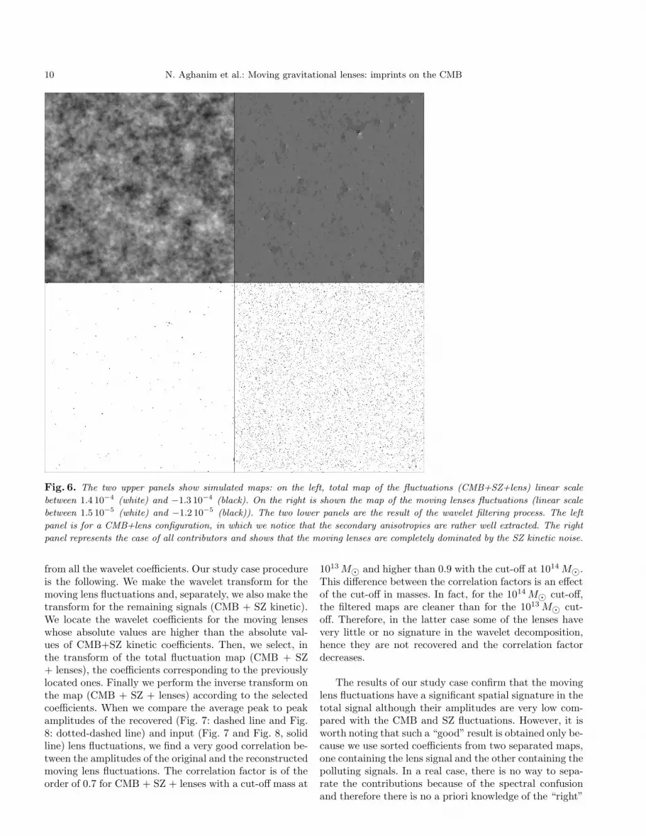
We filter the large scales of a map of CMB+movinglens fluctuations (no SZ kinetic contribution) in order totest the robustness and efficiency of the wavelet trans-form filtering. In this case, the noise due to the CMB isefficiently cleaned. In fact, Figure 6 lower left panel showsa residual signal (symbolised by the dots) associated withthe moving lens fluctuations, which are simulated in theupper right panel of the same figure. We have confirmedthat the positions of the residual signal agree with thepositions of the input structures. Moreover, we were ableto successfully extract the secondary fluctuations due tothe moving lenses, as well as estimate their average peakto peak δT/T values. Figure 8 shows the average peak topeak amplitudes of the input simulated fluctuations (solidline) and the extracted values (dashed line). The mainfeatures are well-recovered, although the amplitudes suf-fer from the smoothing of the filtering procedure. In thisstudy case, with no SZ kinetic contribution, we find a cor-relation coefficient between input and recovered values ofabout 0.95.

Realistic case

When this method is applied to filter a map contain-ing all contributions (CMB + SZ kinetic + moving lenses),we are no longer able to identify or locate the moving lensfluctuations, as shown in fig.6 lower right panel. Here, theCMB which dominates at large scales is cleaned, whereasthe SZ kinetic effect, which is mainly a point-like domi-nated signal, at least one order of magnitude larger thanthe power of the moving lenses, is not cleaned and remainsin the filtered signal. We have filtered at several angularscales without any positive result. On large scales the ex-tended dipole patterns are polluted by the CMB, as men-tioned above, and on small scales the SZ kinetic fluctua-tions are of the same scale as the moving lens anisotropies.We also tried the convolution of the total map (CMB + SZkinetic + moving lenses) with the dipole pattern functionbut we were still unable to recover the moving lens fluctu-ations. In fact, the combination of two SZ kinetic sources,one coming forward and the other going backward, mimicsa dipole-like pattern. In order to distinguish between anintrinsic dipole due to a lens and a coincidence, one needsto know a priori the direction of the motion which is ofcourse not possible. During our analysis, we investigatedtwo cases for the cut off in mass as describe in Sect 4.1.For the simulations with cut-off mass 1014 M⊙ the result-ing background due to point-like SZ fluctuations is lowerthan the cut-off at 1013 M⊙ case; but we were still unableto recover the moving lens fluctuations.

In our attempt at taking advantage of the spatial sig-nature of the moving lens fluctuations, we have located thecoefficients in the wavelet decomposition that are princi-pally associated with the moving lenses and selected them


Fig. 6. The two upper panels show simulated maps: on the left, total map of the fluctuations (CMB+SZ+lens) linear scale

between 1.4 10−4 (white) and −1.3 10−4 (black). On the right is shown the map of the moving lenses fluctuations (linear scale

between 1.5 10−5 (white) and −1.2 10−5 (black)). The two lower panels are the result of the wavelet filtering process. The left

panel is for a CMB+lens configuration, in which we notice that the secondary anisotropies are rather well extracted. The right

panel represents the case of all contributors and shows that the moving lenses are completely dominated by the SZ kinetic noise.

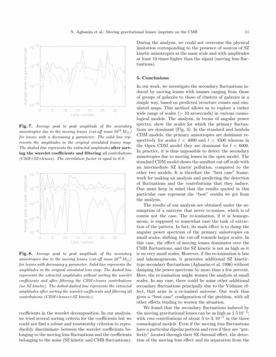
from all the wavelet coefficients. Our study case procedureis the following. We make the wavelet transform for themoving lens fluctuations and, separately, we also make thetransform for the remaining signals (CMB + SZ kinetic).We locate the wavelet coefficients for the moving lenseswhose absolute values are higher than the absolute val-ues of CMB+SZ kinetic coefficients. Then, we select, inthe transform of the total fluctuation map (CMB + SZ+ lenses), the coefficients corresponding to the previouslylocated ones. Finally we perform the inverse transform onthe map (CMB + SZ + lenses) according to the selectedcoefficients. When we compare the average peak to peakamplitudes of the recovered (Fig. 7: dashed line and Fig.8: dotted-dashed line) and input (Fig. 7 and Fig. 8, solidline) lens fluctuations, we find a very good correlation be-tween the amplitudes of the original and the reconstructedmoving lens fluctuations. The correlation factor is of theorder of 0.7 for CMB + SZ + lenses with a cut-off mass at

1013 M⊙ and higher than 0.9 with the cut-off at 1014 M⊙.This difference between the correlation factors is an effectof the cut-off in masses. In fact, for the 1014 M⊙ cut-off,the filtered maps are cleaner than for the 1013 M⊙ cut-off. Therefore, in the latter case some of the lenses havevery little or no signature in the wavelet decomposition,hence they are not recovered and the correlation factordecreases.

The results of our study case confirm that the movinglens fluctuations have a significant spatial signature in thetotal signal although their amplitudes are very low com-pared with the CMB and SZ fluctuations. However, it isworth noting that such a “good” result is obtained only be-cause we use sorted coefficients from two separated maps,one containing the lens signal and the other containing thepolluting signals. In a real case, there is no way to sepa-rate the contributions because of the spectral confusionand therefore there is no a priori knowledge of the “right”


Fig. 7. Average peak to peak amplitude of the secondary

anisotropies due to the moving lenses (cut-off mass 1014 M⊙)

for lenses with a decreasing y parameter. The solid line rep-

resents the amplitudes in the original simulated lenses map.

The dashed line represents the extracted amplitudes after sort-

ing the wavelet coefficients and filtering all contributions

(CMB+SZ+lenses). The correlation factor is equal to 0.9.

Fig. 8. Average peak to peak amplitude of the secondary

anisotropies due to the moving lenses (cut-off mass 1013 M⊙)

for lenses with decreasing y parameter. Solid line represents the

amplitudes in the original simulated lens map. The dashed line

represents the extracted amplitudes without sorting the wavelet

coefficients and after filtering the CBM+lenses contributions

(no SZ kinetic). The dotted-dashed line represents the extracted

amplitudes after sorting the wavelet coefficients and filtering all

contributions (CBM+lenses+SZ kinetic).

coefficients in the wavelet decomposition. In our analysis,we tried several sorting criteria for the coefficients but wecould not find a robust and trustworthy criterion to repro-ducibly discriminate between the wavelet coefficients be-longing to the moving lens fluctuations and the coefficientsbelonging to the noise (SZ kinetic and CMB fluctuations).

During the analysis, we could not overcome the physicallimitation corresponding to the presence of sources of SZkinetic anisotropies at the same scale and with amplitudesat least 10 times higher than the signal (moving lens fluc-tuations).

5. Conclusions

In our work, we investigate the secondary fluctuations in-duced by moving lenses with masses ranging from thoseof groups of galaxies to those of clusters of galaxies in asimple way, based on predicted structure counts and sim-ulated maps. This method allows us to explore a ratherwide range of scales (> 10 arcseconds) in various cosmo-logical models. The analysis, in terms of angular powerspectra, show the scales for which the primary fluctua-tions are dominant (Fig. 3). In the standard and lambdaCDM models, the primary anisotropies are dominant re-spectively for scales l < 4000 and l < 4500 whereas inthe Open CDM model they are dominant for l < 6000.In practice, it is thus impossible to detect the secondaryanisotropies due to moving lenses in the open model. Thestandard CDM model shows the smallest cut-off scale withan intermediate SZ kinetic pollution, compared to theother two models. It is therefore the “best case” frame-work for making an analysis and predicting the detectionof fluctuations and the contributions that they induce.One must keep in mind that the results quoted in thisparticular case represent the “best” results we get fromthe analysis.

The results of our analysis are obtained under the as-sumption of a universe that never re-ionises, which is ofcourse not the case. The re-ionisation, if it is homoge-neous, is supposed to somewhat ease the task of extrac-tion of the pattern. In fact, its main effect is to damp theangular power spectrum of the primary anisotropies onsmall scales, shifting the cut-off towards larger scales. Inthis case, the effect of moving lenses dominates over theCMB fluctuations, and the SZ kinetic is not as high as itis on very small scales. However, if the re-ionisation is lateand inhomogeneous, it generates additional SZ kinetic-type secondary fluctuations (Aghanim et al. 1996) withoutdamping the power spectrum by more than a few percent.Here, the re-ionisation might worsen the analysis at smallscales. In any case, there could be some other additionalsecondary fluctuations principally due to the Vishniac ef-fect, that arise in a re-ionised universe. Our work thusgives a “best case” configuration of the problem, with allother effects tending to worsen the situation.

We found that the secondary fluctuations induced bythe moving gravitational lenses can be as high as 1.5 10−5;with rms contributions of about 5 to 3. 10−7 in the threecosmological models. Even if the moving lens fluctuationshave a particular dipolar pattern and even if they are “per-fectly” located through their SZ thermal effect, the detec-tion of the moving lens effect and its separation from the


SZ kinetic and primary fluctuations are very difficult be-cause of the very high level of confusion, on the scales ofinterest, with the point–like SZ kinetic anisotropies andbecause of spectral confusion.

We nevertheless analysed the simulated maps using anadapted wavelet technique in order to extract the movinglens fluctuations. We conclude that the contribution of the

secondary anisotropies due to the moving lenses is thus

negligible whatever the cosmological model. Therefore it

will not affect the future CMB measurements except as

a background contribution. We have highlighted the fact

that the moving lens fluctuations have a very significant

spatial signature but we did not succeed in separating this

contribution from the other signals.

Acknowledgements. The authors wish to thank J.-L. Puget formany suggestions and fruitful discussions. They wish to thankthe referee, M. Birkinshaw, for his helpful comments that muchimproved the paper. The authors thank J.F. Navarro, C. Frenkand S.D. White for kindly providing us a FORTRAN routine,computing the concentrations and the critical densities of thedark matter profiles, and J.R. Bond for providing the CMBmap used in the analysis. The power spectra of the primaryfluctuations were performed using the CMBFAST code (M.Zaldarriaga & U. Seljak). In addition, we thank F. Bernardeau,F.-X. Desert, Y. Mellier and J. Silk for helpful discussions andA. Jones for his careful reading of the paper.

References

Aghanim, N., Desert, F.-X., Puget, J.-L., Gispert, R. 1996,A&A, 311, 1

Aghanim, N., De Luca, A., Bouchet, F.R., Gispert, R., Puget,J.-L. 1997, A&A, 325, 9

Bahcall, N.A. 1988, ARA&A, 26, 631Bahcall, N.A., Cen, R., Gramann, M. 1994, ApJ, 430, 13Barbosa, D., Bartlett, J.G., Blanchard, A., Oukbir, J. 1996,

A&A, 314, 13Birkinshaw, M. 1989, in Moving Gravitational lenses, p. 59,

eds. J. Moran, J. Hewitt & K.Y. Lo; Springer-Verlag, BerlinBirkinshaw, M. 1997, preprintBirkinshaw, M., Gull, S.F. 1983, Nature, 302, 315Blandford, R.D., Kochanek, C.S. 1987, ApJ, 321, 658Bouchet, F.R., Bennett, D.P., Stebbins, A. 1988, Nature, 335,

410Carroll, S.M., Press, W.H., Turner, E.L. 1992, ARA&A, 30,

499Daubechies, I. 1988, Commun. Pure Appl. Math., vol. XLI,

909Dodelson, S., & Jubas, J.M. 1995, ApJ, 439, 503Ebeling, H., Edge, A.C., Fabian, A.C., Allen, S.W., Crawford,

C.S., Bohringer, H. 1997, ApJ Lett., 479, 101Eke, V.R., Cole, S., Frenk, C.S. 1996, M.N.R.A.S., 282, 263Giovanelli, R., Haynes, M.P., Wegner, G., Da Costa, L.N.,

Freudling, W., Salzer, J.J. 1996, ApJ, 464, 99Grossmann, A., Morlet, J. 1984, SIAM J. Math. Anal., 15, 723Henry, J.P., Arnaud, K.A. 1991, ApJ, 372, 410Hernquist, L., 1990, ApJ, 356, 359Hudson, M.J. 1994, M.N.R.A.S., 266, 468Huss, A., Jain, B., Steinmetz, M. 1997, astro-ph/9703014

Kaiser, N. 1982, M.N.R.A.S., 198, 1033Kaiser, N., Stebbins, A. 1984, Nature, 310, 391Kamionkowski, M., Spergel, D.N., Sugiyama, N. 1994, ApJ

Lett., 426, 57Lacey, C., Cole, S. 1993, M.N.R.A.S., 262, 627Lahav, O., Rees, M.J., Lilje, P.B., Primack, J.R. 1991,

M.N.R.A.S., 251, 128Mallat, S. 1989, IEEE Trans. Patt. Anal. Machine Intell., 7,

674Martinez-Gonzalez, E., Sanz, J.-L., & Silk, J. 1990, ApJ, 355,

L5Mathiesen, B., Evrard, A.E. 1997, astro-ph/9703176Moscardini, L., Branchini, E., Brunozzi, P.T., Borgani, S., Plio-

nis, M., Coles P. 1996, M.N.R.A.S., 282, 384Navarro, J.F., Frenk, C.S., White, S.D.M. 1996, ApJ, 462, 563Navarro, J.F., Frenk, C.S., White, S.D.M. 1997, ApJ, 490, 493Oukbir, J., Bartlett, J.G., Blanchard, A. 1997, A&A, 320, 365Peebles, P.J.E. 1980, in The Large Scale Structure of the Uni-

verse, Princeton University PressPeebles, P.J.E. 1993, in Principles of Physical Cosmology,

Princeton University PressPress, W., Schechter, P. 1974, ApJ, 187, 425Rees, M.J., Sciama, D.W. 1968, Nature, 511, 611Rephaeli, Y. 1995, ARA&A, 33, 541Sachs, R.K., Wolfe, A.M. 1967, ApJ, 147, 73Seljak, U. 1996, ApJ, 463, 1Smoot, G., et al., 1992, ApJ, 396, 1Sunyaev, R.A., Zeldovich, Ya.B. 1972, A&A, 20, 189Sunyaev R.A., Zeldovich, Ya.B. 1980, M.N.R.A.S. , 190, 413Tuluie, R., Laguna, P. 1995, ApJ Lett., 445, L73Tuluie, R., Laguna, P., Anninos, P. 1996, ApJ, 463, 15Viana, P.T.P., Liddle, A.R. 1996, M.N.R.A.S., 281, 323Villasenor, J.D., Belzer, B., Liao, J. 1995, IEEE Trans. Im.

Proc., 8, 1057Vishniac, E. T. 1987, ApJ, 322, 597White, S.D.M., Efstathiou, G., Frenk, C.S. 1993, M.N.R. A.S.,

262, 1023

http://arXiv.org/abs/astro-ph/9703014

http://arXiv.org/abs/astro-ph/9703176

Documents

Moving Gravitational Lenses: imprints on the CMB