1

Moving with the times: baseline data to gauge future shifts in vegetation

and invertebrate altitudinal assemblages due to environmental change.

Organisms, Diversity and Evolution:

International Biodiversity Observation Year (IBOY) special volume.

Niall E. Doran 1, Jayne Balmer1, Michael Driessen1, Richard Bashford2, Simon Grove2,

Alastair M.M. Richardson3, Judi Griggs2, & David Ziegeler1,2

1 Nature Conservation Branch, Department of Primary Industries, Water and Environment, GPO Box

44, Hobart, Tasmania 7001, AUSTRALIA.

2 Forestry Tasmania, GPO Box 207, Hobart, Tasmania 7001, AUSTRALIA.

3 School of Zoology, University of Tasmania, GPO Box 252-05, Hobart, Tasmania 7001,

AUSTRALIA.

Corresponding author

Dr N.E. Doran, Nature Conservation Branch, Department of Primary Industries, Water and

Environment, GPO Box 44, Hobart, Tasmania 7001, AUSTRALIA. fax Australia 3 6233 3477, phone

Australia 3 6233 3627, email Niall.Doran@dpiwe.tas.gov.au

ABSTRACT

A long term monitoring program has been established in Tasmania, Australia, as a Satellite

Project for the International Biodiversity Observation Year (IBOY). This program aims to

monitor distributional change in vegetation and fauna assemblages along an altitudinal

2

gradient (70-1300m) in response to climate change and other environmental events. Baseline

data collected over a two year period will be available for comparison with data collected in

future decades.

The vegetation varies with altitude and fire history. The rate of change in vegetation is

not continuous along the altitudinal gradient, but is most rapid above 700 m and below the

treeline at 1000-1100 m. Most vascular plant species reach the limit of their distribution

within this zone.

Despite its preliminary nature, the invertebrate data also display altitudinal and

seasonal patterns. The tree line and the 700-1000 m zone again appear to be notable in terms

of invertebrate distribution. While the composition of ground-based taxa may be closely

related to the floristic composition of the vegetation (or its environmental drivers), the

airborne invertebrate fauna appears to be more closely related to structural characteristics

such as height and density. Of all taxa, the Coleoptera appear to be the best potential

indicators across most altitudes and times.

Although the current data provide a wealth of inventory and distributional information

over altitude, their greatest potential value lies in long term comparative information. Future

sampling should focus not only on changes at and above the treeline, but also on the zone

below this where many species are at their altitudinal limits and may be particularly sensitive

to climate change.

Key words: Climate change, long-term monitoring, altitudinal gradient, biodiversity, plant

species assemblage and invertebrate assemblage.

3

Introduction

Climate change poses a significant potential problem for the long-term management of

reserves and protected areas. The effects of climate change are predicted to include dramatic

change in rainfall level and geographic coverage, change in temperature and fire risk,

increases in the frequency and severity of extreme climatic events such as storms, droughts

and floods, and a rise in sea level (CSIRO 1996, IPCC 1996, IPCC 2001a&b).

Less dramatic, but no less serious, effects of climate change may include changes in

prevailing environmental conditions that directly or indirectly affect the ability of species to

survive and flourish within their natural range. The future adequacy of existing reserves and

management is therefore a critical issue, as climate change may reduce or alter the

distribution of flora and fauna within and beyond the geographic or altitudinal boundaries in

which they are currently protected (Hughes & Westoby 1994, Parmesan 1996, Gascon et al.

2000).

The immediate effects of climate change in forested regions are likely to produce

changes in ecosystem function and processes governing community composition and

structure, followed by shifts in tree line margins and boundaries between forest types and

ecotones (Luckman & Kavanagh 2000, Hilbert et al. 2001, Klasner & Fagre 2002, Kullman

2002). Change in geographic, altitudinal, and seasonal patterns within biota is likely to

accelerate, and some researchers have indicated that future changes in biodiversity may occur

at the landscape level in as little time as decades (Hannah et al. 2002). Predictive models

have indicated that large changes in forest distribution and extent may occur with even minor

climate change (Hilbert et al. 2001). For instance, over three quarters of Canadian National

Parks may experience shifts in dominant vegetation as atmospheric carbon dioxide levels

increase (Hannah et al. 2002).

4

The large (35-240km) northern geographic shift observed in the distribution of 63% of

non-migratory European butterflies alone over the last century (as compared to 3% shifting

south) provides a marked example of the scale of potential climate-change effects not only

over single species but a broad taxonomic group (Parmesan et al. 1999). Such distributional

changes will not only affect animal taxa of conservation significance, but also beneficial and

pest species as well (Harrington et al. 2001).

Because of these concerns, a joint project has been established between the

Tasmanian Department of Primary Industries, Water and Environment (DPIWE), Forestry

Tasmania and the University of Tasmania to record baseline inventory and distributional

biodiversity data against which future changes in the altitudinal distribution of flora and fauna

can be measured (Brown et al. 2001). Long term monitoring plots were established in 1999-

2000 across an altitudinal gradient within the Warra Long Term Ecological Research Site

(LTER; Figure 1), in order to study changes over time in relation to climate change,

succession due to fire or its absence, and other chance events. Warra is a core site within the

International Biodiversity Observation Year (IBOY) global long term monitoring network,

and the altitudinal transect surveys have been supported as an associated Satellite Project.

The vegetation within the research site varies from lowland wet forests through

scrubby subalpine woodlands to alpine heaths. The wet forests vary from climax cool

temperate rainforest dominated by Nothofagus cunninghamii (Hook.) Oersted to various

sclerophyllous fire sere communities dominated by the genus Eucalyptus (Corbett and

Balmer 2001).

Previous workers studying Tasmanian vegetation have noted that the rate of floristic

change is not constant over the altitudinal gradient (Ogden & Powell 1979, Noble 1981,

Kirkpatrick & Brown 1987, Pyrke 1989, Bridle & Kirkpatrick 1994, Kirkpatrick et al. 1996).

Such discontinuities in species richness have been recognised globally in both flora and fauna

5

(Rahbek 1995, Sanders 2002), and both the tree line and the level of the cloud/mist layer may

play an important role in some of these patterns (Kirkpatrick et al. 1996, Pounds et al. 1997,

Hilbert et al. 2001).

The primary focus of this study is an analysis of relationships between the altitudinal

gradient and the associated transition in biodiversity. This paper examines the variation in

vascular plant and invertebrate richness identified in the preliminary stages of the long-term

project. Because the work is ongoing, invertebrate information is currently only available at

an ordinal level, but taxonomic resolution will be refined to a finer level as the data become

available.

Methods

Survey design

Overviews of the Warra study site, in south-west Tasmania, and the initial set-up of the

altitudinal study are provided in Brown et al. (2001) and Bashford et al. (2001). The study

reported here consists of four transects covering a combined altitudinal range from 70m to

1300m above sea level (Figure 1). Half of the site is within the Tasmanian Wilderness World

Heritage Area, representing a natural area that has never been logged. The remainder of the

site is within State forest, some of which has undergone a single logging event.

Plots were established along each transect at approximately 100 m elevational

intervals, but the altitudinal range sampled by each transect varied. Transect A and C sampled

elevations from 100 to 600 m inclusive, transect B sampled elevations between 100 and 300

m inclusive, and transect D sampled from 500 to 1300 m inclusive. Sampling at high altitudes

was constrained by access. As far as possible, plots were selected to minimise environmental

heterogeneity in terms of geology, aspect and slope (Table I in electr. suppl.). Plots differed

in their disturbance histories, due to wildfire and logging. All four transects were used to

6

collect the vegetation data. Due to funding constraints only two transects were used to sample

invertebrates. The transects with the least disturbance history but greatest altitudinal range

were chosen, in order to reduce the number of factors studied while maximising potential

differences in those that remained.

For each plot, a permanent 50 x 20 m grid was established, as outlined in Bashford et

al. (2001). The plot was divided into ten 10x10 m subplots following the standard procedure

adopted for Permanent Forest Inventory plots established throughout Tasmania.

Floristic surveys

Within each subplot, the species and diameters of all trees greater than 10 cm in diameter at

breast height were recorded and their location was mapped. The general structure of the

vegetation was described for each subplot and each vascular species was recorded together

with an estimate of its cover, using a modified Braun-Blanquet index (Table II in electr.

suppl.). Stand structure variables were derived from this data to provide number of trees

(NoTrees), number of eucalypts (NoEucs), and maximum eucalypt diameter (MaxDBH).

Frequency (number of subplots in which a species was present) and average cover

(Braun-Blanquet class mid-values) were used to determine species importance values (IV) for

each plot. The IV was calculated by adding the relative frequency and relative cover of the

species for the plot (Mueller-Dombois & Ellenberg 1974). The percentage IV of rainforest

trees (IVRFt) was calculated by adding the scores for all rainforest trees (sensu Jarman and

Brown 1983) and dividing by the total score for all trees. Similarly, a percentage IV for

rainforest woody plants (using shrubs and trees) was also calculated for each plot (IVRF).

Relative abundance of each species was used to calculate percentage cover scores for trees,

shrubs, herbs, climbers, graminoids and ferns. Mean species richness (mSppRich) was

calculated by averaging the total species count for each subplot across each plot, and the total

7

species number was also tallied. The direction that the slope was facing (Aspect) was

measured using a compass recorded in degrees from North, the steepness (Slope) was

measured using an inclinometer and also recorded in degrees and the area of exposed rock

(Rock cover) was estimated as a percentage of the total plot area.

No accurate disturbance history has been compiled for the plots, although recent fires

and logging are documented. Crude estimates have therefore been made on the approximate

timing of past fire events using stand structure information (tree diameters and densities),

information from Forestry Tasmania PI mapping (1984 and 1948), fire history mapping

(Hickey et al. 1999), and comparisons with stand age structure reported for other sites within

the Warra (Alcorn et al. 2001). Variables relating to disturbance were ‘logged’ (1 = logged

once, 0 = not logged); estimated years since last fire (‘YSLF’); estimated age of the oldest

trees in the plot (‘OldAge’); and estimated number of fires in the past 500 years (‘FireFreq’).

Fire frequency is likely to have been underestimated, as some recent fires may have

destroyed all trees originating from previous events in the past 500 years.

Invertebrate surveys

Pitfall traps

Six pitfall traps were established in each grid for transects A and D, with the exception of the

500m site on Weld transect D (omitted due to time constraints for remote area work). These

were arranged in a regular pattern in each grid (Bashford et al. 2001), with exact pitfall

location depending on the ease of measurement on the terrain and the availability of

sufficiently deep soil/substrate in which to set the trap.

As described in Bashford et al. (2001), standard pitfall traps consisted of a 15cm

length sleeve of 9cm diameter PVC stormwater pipe sunk vertically into augered holes in the

soil. (At the 100m site, soil was insufficiently deep and soil and rock needed to be built up

8

around the PVC sleeve). A 425ml plastic cup of matching diameter was fitted within each

sleeve. To prevent rain and debris entering the cups directly, plastic food container lids were

supported 3 cm above the cups on bamboo skewers. Each cup was filled with 100ml of either

33% (353 g/l) ethylene glycol for sheltered sites (below the tree line: 100m – 1000m) or

undiluted (1075g/l) ethylene glycol for exposed sites (above the tree line: 1100m – 1300m).

In the last two months of the study, 5% glycerine/glycerol was added to the pitfall mix to

improve the condition of specimens recovered for identification.

Malaise traps

Malaise traps were established at every second grid below the tree line, with an additional

trap at the lowest altitude (100m, 200m, and 400m on transect A; 600m, 800m and 1000m on

transect D). Malaise traps were placed within each grid at a location where suitable trees were

available to hang them in the path of flying insects.

Malaise traps consisted of a 28-gauge Terylene mesh tent with dark central panels and

a light-coloured sloping roof, leading to a collection bottle containing 70% ethanol. The

fragile nature of malaise traps made them unsuitable for use in the exposed conditions above

the tree line (1100m-1300m).

Sampling schedule

Transect A was readily accessible from a forestry road. Transect D, however, was very

remote. In order to restrict sampling to a manageable time-frame, helicopter transport was

used to access the 1200m site, with sampling teams proceeding to 1300m and then walking

back down the ridge and collecting samples on their way. Sampling periods were chosen

from October to April, to take advantage of greater net invertebrate abundance and diversity,

generally better weather conditions, and longer days to complete sampling requirements.

9

Pitfalls within transect A were established and allowed to settle in late December

2000. Access issues and costs prevented this from occurring on transect D, and so pitfalls and

malaise traps were established and opened over a three-day period in late January 2001.

Transect A pitfalls were opened and malaise traps were established the day after those for

transect D sites were completed.

Subsequent collection and re-setting of traps was nominally based on a four-week

cycle. In practice, exact sampling dates were determined by flying conditions for the

helicopter. For this reason, sampling was driven by access to the higher altitude sites, with the

first day spent clearing and re-setting transect D, and the second spent clearing and resetting

transect A.

Pitfall traps were cleared by filtering the ethylene glycol through a 0.9x0.3mm mesh,

and resuspending the mesh in 70% alcohol. Pitfalls were then recharged with fresh ethylene

glycol. Malaise traps were cleared and reset by simply replacing the collection bottle with a

new one. All waste ethylene glycol and alcohol was removed from the sites.

Samples were collected at the end of February, March and April 2001, before traps

were closed over winter and re-set at the end of October 2001. Second season samples were

taken at the end of November and December 2001, and January 2002. Additional samples

were also taken in February, March and April 2002, for comparison to the first sample period,

but these are yet to be sorted.

All animal material from both pitfalls and malaise traps was sorted under a stereo

dissecting microscope in the laboratory. Initial sorting identified and quantified all material to

the ordinal level. This material will be identified in greater detail, with specific groups

targeted for further work.

10

Taxonomy

Vascular plant species nomenclature follows Buchanan (1999). Finer level taxonomic

resolution for the invertebrates is currently underway and is not reported in this paper.

Data analysis

The vascular species present for each 100 m elevation class were compiled and analysed to

determine the floristic dissimilarity between each adjacent class. The results were graphed

using Jaccards similarity index (Mueller-Dombois and Ellenberg 1974). An association

matrix was generated from the presence/absence data for these altitudinal classes in PATN

(Belbin 1995) using the Czenowski/Bray-Curtis distance measure, and the dissimilarity

between each altitude class was also graphed. In addition to graphing the sampled species

richness for each altitude class, the interpolated species richness was generated by extending

species distributions into the altitude classes between the lowest and highest classes where

they were recorded to occur.

The vegetation data were divided into two subsets for multivariate analysis. All plots

across the complete altitudinal range sampled from transects A and D were analysed as one

set, despite a recognition that the large beta diversity within this altitudinal range potentially

violated the conditions for ordination. To compensate, the lowland forest plots from all

transects (below 800 m altitude) were re-analysed as a second set meeting all the conditions

of the ordination.

Plant species represented by only one sub-plot were excluded from the multivariate

analysis. Some species could not be identified to species level and were included as species

groups.

For invertebrates, the ordinal level data compiled to date were analysed to provide an

overview of the broad-level taxonomic patterns occurring along transects A and D. These

11

patterns will be resolved in more detail as the taxonomic resolution of the analysis is

improved in future work.

Pitfall and malaise trap data were treated separately, as were data from the two

different invertebrate sampling periods: February to April 2001 (series 1, 2 and 3) and

November 2001 to January 2002 (series 4, 5 and 6). Data for each month were kept separate

within each analysis to detect any time-based change over the respective three-month period.

Pitfall data were averaged from the six pitfall traps per site per date. Malaise trap data consist

of the single malaise trap catch for each relevant altitude. Data analysis was as inclusive as

possible, but vertebrate by-catch, invertebrate larval forms, and particularly rare or unusual

groups (e.g. emergent parasitic worms) were excluded.

Data were primarily analysed using the PC-Ord for Windows Multivariate Analysis of

Ecological Data package (McCune & Mefford 1999). Ordination used non-metric multi-

dimensional scaling (MDS/NMS), with the Sorenson (Bray-Curtis) distance measure for the

association matrix.

Because the significance of the associations between individual variables and the

ordination scores is not testable within PC-Ord, the vegetation data was also analysed in the

software package ‘PATN’ (Belbin 1995) using the ordination technique semi-strong-hybrid

multi-dimensional scaling (SSH: Belbin 1992). The environmental variables were correlated

with the results of the ordination using Principle Axis correlation Analysis (PCC: Belbin

1995). The significance of the associations was then tested using a Monte Carlo

Randomisation technique (Manly 1991), and the statistical package ‘Statgraphics’

(Manugistics 1997) was also used for multivariate regression analysis.

Given the broad ordinal level basis of the invertebrate data, environmental

associations were treated as indicative at this stage, and not subjected to as rigorous an

analysis. Invertebrate site-species matrices were subjected to logarithmic transformation to

12

reduce the influence of numerically dominant groups, and plotted in ordination space using

MDS. Three basic environmental variables – altitude (100-1300m), transect line (A or D) and

date (February-April or November-January) – were overlaid as vectors on these ordinations.

Cluster analysis (Ward’s Method, using the Euclidean Distance Measure) was

undertaken to clarify and confirm site groups emerging from the invertebrate ordination

patterns. Multi-Response Permutation Procedures (MRPP) was undertaken to determine

significant differences between these ‘observed’ cluster groups, and Indicator Species

Analysis (ISA) was then used to identify the invertebrate taxa contributing most to the

distinction between them. ISA was also used to identify corresponding patterns in vegetation

characteristics associated with the determined groups, and vice versa.

Preliminary analysis of pitfall data indicated a major distinction between the high

altitude sites (1100-1300m, above the tree-line) and all others. Analyses were undertaken

using all site data to demonstrate this marked altitudinal separation, and were then repeated

without the three high altitude sites in order to assess patterns below the tree-line in more

detail.

In some cases, pitfall numbers were reduced due to animal disturbance or flooding.

Lyrebirds (an introduced species in Tasmania) in particular caused disruption at 600m and (to

a lesser degree) 700m on transect D, and at 300-400m on transect A. As noted in the

following section, outliers from 600-700m on transect D were excluded from analysis in

some cases, often because they represented averages from a low number of remaining pitfalls.

Results

Floristic surveys

Plant Diversity

13

A total of 155 vascular plant species (Table III in electr. suppl.) were recorded within 24 plots

(all 0.1 ha). This represents 60% of the vascular species recorded from the Warra LTER site

to date (Corbett and Balmer 2001). The diversity of cryptophytes exceeds that of the vascular

plant flora but is not examined here. Jarman and Kantvilas’s (2001) study of bryophytes and

lichens within the Warra LTER recorded 144 species of bryophytes and 134 species of lichen

from only 9 wet Eucalyptus obliqua L'Hérit plots that were half the size of those in the

current study.

Figure 2 shows the relationship of species richness (recorded in 50 x 20 m plots) and

mean species richness (10 x10 m subplots) with the altitude gradient on Mt Weld. The

percentage importance value (IV) of rainforest species (dominance) is also plotted as an

indication of disturbance history for each plot. The total species richness of vascular plants

was highest (51) for a lowland plot burnt in the 1934 fires (A03). This plot is now occupied

by both sclerophyllous and rainforest species and therefore has an intermediate value for

rainforest importance. High and low scores for the importance value of rainforest were

associated with low values of species richness. Figure 1 in the electronic supplement shows a

second order polynomial model, in which the importance value of rainforest species explains

52% of the total species richness (P<0.001).

There is no significant linear relationship in total species richness with altitude. A

second order polynomial model was significant in explaining 36% of the variation in total

species richness (P<0.01; Figure 2 in electr. suppl.), but the relationship is weak.

When looking at species richness in the smaller sub-plots, mean vascular plant species

richness (Figure 2) was greatest in the alpine plot D12, with an average of 28 species within

0.01 ha subplots. There is a significant positive linear relationship between altitude and mean

species richness (P<0.02) with 23% of the variation in mean species richness explained by

altitude. The polynomial relationship was stronger, explaining 38 % of the variation in mean

14

species richness (P<0.007; Figure 3 in electr. suppl.). No other individually tested

environmental variable was significantly correlated with mean species richness (P>0.05), but

60% of the variability was explained using a multiple regression model combining altitude,

fire frequency, oldest age and estimated years since last fire (P<0.01 for all variables).

Analysis of vascular plant species richness in terms of plant life forms provides both

positive and negative correlations with altitude (Figure 4 in electr. suppl.). Trees have a

strong negative correlation with altitude (P<0.001), which explains 69% of the variation in

tree species richness. Ferns also have a strong negative correlation with altitude (P<0.001),

explaining 55% of the variation in species richness. In contrast, there is a positive correlation

between altitude, non-tree woody plants and both monocot and dicot herb groups (P<0.001,

P<0.005 and P<0.001), explaining 58%, 30% and 41% of the variation, respectively.

Figure 3 presents the species data merged into 100 m altitudinal classes. This chart

shows a different relationship between species richness and altitude. In this case there is a

negative correlation between the interpolated species richness (P < 0.003), but not with

sampled species richness. Altitude explained 58% of the variation in interpolated species

richness. The total numbers of species reaching their limits in each altitudinal class is plotted

in Figure 3, and shows that the greatest percentage of species change-overs takes place at 600

m and 1000 m elevation. Lower but moderate rates of change take place between these two

altitudes. Figure 3 also shows the dissimilarity scores between adjacent altitude classes. The

highest dissimilarity is between 700 and 800 m. A more detailed graph of dissimilarities is

presented in Figure 5 in the electronic supplement. This figure shows that the degree of

dissimilarity is strongly associated with three altitude zones. Plots at 700 m and below have a

high degree of similarity with each other and are least similar to the plots at and above the

tree line (1100 m). The plots at or above the tree line (1100 to 1300 m) are quite similar to

15

each other. A transition zone between the high and low altitude plots occurs between 800 and

1000 m.

Only eight species were represented across the complete altitudinal range from

lowlands to above the treeline. Sixty vascular species (39% of the sampled flora) are

restricted to the top 600 m of the altitude gradient on Mt Weld (800m to 1300 m), compared

with fifty-five species (35%) that were restricted to the lowest 600 m zone (100-600 m). The

total richness is actually slightly higher in the lower zone (94 compared to 87 species), but

the area sampled was nearly double that of the upper zone. When the difference in sampled

area is taken into account using the formula d= S/log of Area (Whittaker 1971), the diversity

of the upper altitude zone is marginally higher (d=23.0 compared with d=22.2). Both

structurally and floristically, the vegetation above the treeline is distinctive due to the absence

of trees and the greater importance of shrubs, herbs and graminoids.

Floristic patterns

Figure 4 shows ordinations for the two data subsets. In both there is a significant relation

between floristics and altitude (P<0.001) and percentage rock cover (P<0.04), but not

between floristics and slope, drainage or aspect (P>0.05). The disturbance variables tested

were significantly associated with the floristics (P<0.05) for both data sets with the exception

of years since last fire, which was not significant for the subset that included all altitudinal

plots from transects A & D. The structural attributes of the vegetation (such as percentage

cover of trees, shrubs, herbs, graminoids and ferns, tree diameter and density, mean species

richness, and importance value of rainforest taxa and rainforest trees) were all significantly

related with the floristics of the data for transects A& D. However, some of these variables

were not significant for the lowland data set (Max DBH., %cover trees, %cover of herbs and

% cover of ferns were all P >0.05). Basal area was not significant in either data set.

16

The ordination graph in Figure 4a shows the complete altitudinal range of vegetation

from 100-1300 m along transects A and D. Altitude is strongly associated with the first axis

of the ordination and explains 89% of the variation. Fire frequency is also strongly associated

with the first axis of the ordination explaining 68% of the variation. In combination, these

two variables explain 95% of the variation of the first axis. Altitude combined with the age of

the oldest vegetation and percentage rock cover explains 69% of the variation in the second

axis.

Figure 4b shows the result of the ordination of all lowland plots across all four

transects. Multiple regression indicated that fire frequency and logging together explained

65% of the variation in the first axis, with the addition of altitude explaining a further 11%.

Rock cover alone explained 43% of the variation of the second axis.

In Figure 4a, the alpine plots (D11, D12 and D13) located between 1100 and 1300 m

are well separated from the subalpine plots (D10, D09 and D08). The subalpine plots are also

relatively well separated from the lowland forests dominated by Eucalyptus obliqua and E.

delegatensis (Figure 4a). The lower altitude plots are quite dispersed across the ordination

and the relationship with altitude is unclear.

The alpine plots were floristically similar and all contained the heath Richea scoparia

and the lily Astelia alpina as important components. The three subalpine E. coccifera Hook.f.

woodland plots were directly aligned with the vector for altitude, and had an understorey

dominated by rainforest species including Nothofagus cunninghamii and Eucryphia milliganii

Hook.f.

There is a relatively large separation within the ordination between the E. coccifera

woodland plots and the lowland forest plots. Most of these lowland forest plots had an

overstorey dominated by Eucalyptus obliqua, but five plots were dominated or co-dominated

by E. delegatensis Boland. Distinguishing between E. delegatensis and E. obliqua is difficult

17

in some instances, and the two were observed to hybridize where they occur together. Only

one lowland plot (B02) was co-dominated by E. regnans, a species characteristic of fertile

and sheltered lowland sites, but this one was recovering from logging.

The E. delegatensis plots are located midway on the ordination between the E.

obliqua forests and the subalpine E. coccifera forests. This species is known for its greater

cold tolerance than E. obliqua and E. regnans. These plots have a variable understorey

dependent in part on the disturbance history. Some plots had quite a distinctive flora

including species such as Telopea truncata (Labill.) R.Br. Those that have a relatively recent

fire history include Nematolepis squamea (Labill.) Paul G.Wilson, Acacia riceana Henslow

and Leptospermum lanigerum (Aiton) Smith. Those that have not had recent fire had

rainforest understoreys including a distinctive shrub component and the trees Eucryphia

lucida (Labill.) Baill. and Anodopetalum biglandulosum A.Cunn. ex Hook.f.

The dispersion of the lowland E. obliqua forest plots is orthogonal to the trend of

altitude in the ordination space, the variation correlating with disturbance history. Plot A01

and D06 represent the two extremes in the distribution of lowland plots in the ordination. Plot

A01 is a 1934 regrowth plot that has more than two ages of eucalypts suggesting repeated

fires. D06 is an almost pure climax callidendrous rainforest co-dominated by Nothofagus

cunninghamii and Atherosperma moschatum Labill. with an open understorey of the tree fern

Dicksonia antarctica Labill.

Some regrowth forests with relatively high floristic diversity due to the presence of a

dry forest floristic elements occur at the lower altitudes of transect A and B (Plots B01, A01

and A02). This forest was distinguished by the presence of bracken fern, Pteridium

esculentum (Forst.f.) Cockayne, the tall tussock sedges Gahnia grandis (Labill.) S.T.Blake

and/or Lepidosperma ensiforme (Rodway) D.I.Morris, the undershrubs Gonocarpus

teucrioides DC. and Epacris impressa Labill., the climber Hibbertia empetrifolia (DC.)

18

Hoogl., the shrub Lomatia tinctoria (Labill.) R.Br. and the trees Acacia verticillata, Banksia

marginata Cav., Bedfordia salicina (Labill.) DC., Leptospermum scoparium Forst. & Forst.f.

and Notelaea ligustrina Vent.

The more typical lowland wet sclerophyll plots had an understorey of lower diversity

dominated by broad-leaved sclerophyllous species such as Pomaderris apetala Vent. and/ or

Nematolepis squamea, Olearia argophylla (Labill.) Benth., the small shrub Coprosma

quadrifida (Labill.) Robinson and the sedge Gahnia grandis.

In areas where fire has been excluded for sufficient time the resulting mixed forest

understorey was dominated by Nothofagus cunninghamii in association with Atherosperma

moschatum. In forests on more protected sites it tends to be tall and open, with tree ferns in

the understorey along with a high diversity of epiphytic ferns but a low diversity of other

vascular species. Elsewhere the rainforest is more diverse, with Eucryphia lucida and

Anodopetalum biglandulosum being important components of the thamnic or implicate

rainforests (Jarman et al. 1984).

Invertebrate surveys

Invertebrate diversity

Some 204,000 invertebrate specimens have been sorted and identified to the ordinal level,

covering the monthly samples collected from February to April 2001 and from November

2001 to January 2002. Over 150,000 invertebrates were collected in malaise traps during the

two sampling periods representing 21 major taxa (ordinal level and above, Table I). Diptera

comprised 85% of all invertebrates collected. Other groups taken in relatively large numbers

were Hymenoptera (6%), Hemiptera (2%), Lepidoptera (2%), Collembola (2%) and

Coleoptera (1%).

19

Nearly 53,000 invertebrates were collected in pitfall traps representing 22 major taxa.

As was the case for the malaise traps, Diptera accounted for most (42%) specimens collected.

Other taxa taken in relatively large numbers were Mecoptera (19%), Collembola (12%),

Coleoptera (7%), Araneae (5%), Hymenoptera (3%), Amphipoda (3%), Acarina (3%) and

Orthoptera (1%).

Approximately 11,000 more specimens were collected in malaise traps during

November-January than during February-March, largely due to the collection of more Diptera

in the former months. Coleoptera, Collembola, Hemiptera and Lepidoptera were also more

common in November-January. Acarina and Araneae were notably more common in

February-April. As with the malaise traps, the number of specimens collected in pitfall traps

was greater in November, but only by 1,100 specimens. Similarly, the numbers of Diptera,

Coleoptera, Collembola and Hemiptera were also greater in November-January. Araneae,

Blattodea, Formicidae, Isopods, Mecoptera and Orthoptera were more common in pitfalls in

February-April.

The large number of Mecoptera (nearly 10,000) collected in pitfalls in February-April

was of particular interest. This order was predominantly represented by an undescribed large,

wingless alpine species of Apteropanorpa. This genus of scorpion fly has only rarely been

captured, and was believed to only be a winter taxon. The high altitude sites also yielded a

large (1.5-2.5cm) new species of the gastropod genus Victaphanta¸ previously only known

from two specimens collected at high altitude elsewhere in the state, as well as rare elements

amongst the carabid and lucanid beetle fauna that need to be investigated in detail.

Invertebrate patterns – pitfall traps

MDS ordinations for all pitfall data provided three dimensional solutions (stress 0.099 and

0.110 for February-April and November-January, respectively; and 0.117 and 0.104 for the

20

same periods with the high altitude sites removed. Stress values were calculated by Kruskal’s

formula). As outlined before, the three high altitude sites (1100–1300m, D11-D13) tended to

separate distinctly from the others, but the remaining sites also demonstrated clear altitudinal,

transect and date related trends (see overlaid vectors, Figure 5). Because similar patterns were

exhibited in both series of pitfall data and in each dimension of the ordinations, only a

representative example is presented in Figure 5 for the sake of brevity.

Cluster analysis identified clear groupings in keeping with the altitude, transect and

(to a lesser degree) date driven patterns identified by the ordinations. The nature of these

groupings, their significance (as determined via MRPP) and the invertebrate species most

contributing to them (as determined via ISA) are outlined as follows.

Pitfall traps: February to April

The high altitude (1100-1300m) sites from March and April completely separated

from the others (P<< 0.001 via MRPP). The only high altitude sites not within this group

were those from February. Two major groups emerged from the remainder, with the first

composed of low altitude sites (100-500m) from all three months, and the second composed

predominantly of mid to higher altitude sites (600-1000m) from all three months. These two

groups were again significantly different (p<<0.001). [Note that D06 (April) was excluded as

an extreme outlier].

With the removal of the high altitude sites from the ordination and cluster analysis,

three major groups emerged within the below tree-line data (Figure 6a), again showing

predominantly altitudinal and transect driven patterns. The low altitude sites from all three

months remained grouped as before, but this time as significantly different outliers to the

others (P<<0.001). The remaining sites divided into two significantly different groups

(P<0.001), the first consisting of mid- to high-altitude sites for February and predominantly

21

mid-altitude sites for March-April, while the other group consisted predominantly of higher

altitude sites from March-April.

The invertebrate taxa contributing significantly (P<0.05) to the separation of the

highest altitude sites from those below the tree-line were the Araneae, Blattodea, Coleoptera,

Collembola, Dermaptera, Diptera, Formicidae, Isopoda, Lepidoptera, Mecoptera, and

Opiliones (Table II). With the removal of the highest altitude sites from the analysis, the low

altitude sites were distinguished from all others by a predominantly different assemblage

consisting of the Amphipoda, Annelida, Chilopoda, Coleoptera, Diptera, Formicidae, other

Hymenoptera and Thysanoptera. In turn, the predominantly mid and higher altitude groups

were distinguished from each other by only two main taxonomic groups, the Coleoptera and

Collembola.

Although the pitfall data reflected a similar faunal discontinuity around the tree-line

as seen in the floristic data, no distinct discontinuity was directly observed between 700-

800m based on the invertebrate ordinal data alone. Despite this, allocation of 100-700m and

800-1000m sites to different groups did produce a significant difference (P<0.001), driven by

the Araneae, Blattodea, Formicidae and Mecoptera (all P<0.05). Similarly, the floristic data

supported the second major distinction observed in the invertebrate data: the above grouping

of low altitude sites remained significant (P = 0.02) when applied to the floristics, with 40 of

110 plant species significantly contributing to the difference. Interestingly, floristic data were

not significant in separating the mid to higher altitude groups identified through the

invertebrate data (P = 0.1, only 9 of 110 species contributing), most probably because they

bridged the floral discontinuity identified within this range.

22

Pitfall traps: November to January

Ordination and cluster analysis identified four clear groups within the data for pitfall

traps over the second sampling period. High altitude (1100-1300m) and late (January) sites

from transect D significantly separated from all other sites (P<<0.001), followed by a

separation of mid-altitude sites from both transects, again significantly different to the

remaining cluster (p<<0.001). Of the two groups most closely linked, one consisted

predominantly of lower altitude sites from transect A, while the second consisted

predominantly of mid to high altitude (but early season) sites from transect D. These two

groups also separated significantly from each other (P<<0.001).

Removal of the high altitude sites provided a clearer grouping of the remainder

(Figure 6b), although four outliers that had been affected by trap disturbance were also

excluded (site D06 from all months and D07 from November). Four clear groups were again

identified by cluster analysis, in the same general pattern as above. The first three groups

consisted exclusively of transect A sites: all lower altitude (100-200m) for the first,

predominantly higher (300-600m) and later (January) for the second, and predominantly

higher (300m-600m) and earlier (November-December) for the third. The fourth group was

exclusively composed of the remaining transect D sites (700-1000 m). All groups were again

significantly different from the remainder (P = 0.002 for the second, and P<<0.001 for the

third and fourth groups, respectively). Further altitude-based divisions can be seen within

these groupings (Figure 6b).

In common with February-April, the Araneae, Blattodea, Coleoptera, Collembola,

Dermaptera, Diptera, and Opiliones were significant (P<0.05) in distinguishing higher

altitude/later month sites from the others (Table II). In contrast to February-April, however,

the Acarina, Chilopoda, Hemiptera, Orthoptera, and Thysanoptera were also significant,

while the Formicidae, Isopoda, Lepidoptera, and Mecoptera were not.

23

Below the tree-line, the remaining transect D sites (700-1000 m) were distinguished

from transect A by a mix of the Amphipoda, Araneae, Collembola, Formicidae, Mecoptera,

Opiliones and Orthoptera. Mid-altitude and earlier month samples from transect A were also

separated from the others by the Amphipoda, Araneae, Collembola and Formicidae, but with

the other groups replaced by the Acarina, Coleoptera, Hemiptera, and other Hymenoptera.

The remaining low altitude and mid-altitude/later month transect A sites were separated from

each other by the Acarina, Coleoptera, Diplopoda, Diptera, Isopoda, and Lepidoptera; again,

a largely different assemblage to that separating the lower altitude sites for the February to

April period.

The 700-800m floristic discontinuity was reflected in the invertebrate data for pitfall

traps from November-January, with the 700-1000m sites separating distinctly from those

below. The discontinuity is obscured, however, by the absence of data from the D06 (600m)

sites for this period. Separation of the invertebrate data into 100-700m and 800-1000m sites

again provided a significant difference between groups (P<<0.001), however, this time driven

by the Amphipoda, Araneae, Blattodea, Collembola, Formicidae, Mecoptera, Opiliones and

Orthoptera (all P<0.05). Most of these groups, with the exception of the Blattodea, were

responsible for the invertebrate pattern already described above.

Not surprisingly, the floristic data strongly supported the invertebrate-based

distinction between transects A and D (P<<0.001). This support was most likely to have been

driven by the observed floral discontinuity, with 73 of 108 plant species contributing to it

(P<0.05). Floristic data did not support the separation of mid-altitude/earlier month sites from

transect A (P = 0.08; 18 of 108 species contributing), but did support the separation of low

altitude from mid-altitude/later month sites (P = 0.01, 27 of 108 species contributing).

24

Invertebrate patterns - malaise traps

Due to the impracticalities of establishing malaise traps at the high altitude sites, these data

are not complicated by a sharp discontinuity based around the tree line. MDS ordinations

provided a three dimensional solution (stress 0.050) for February-April, and a two

dimensional solution (stress 0.075) for November-January. As with the pitfall data, only a

representative example of the ordination patterns for the malaise trap data is presented in

Figure 7 for the sake of brevity. Altitude and transect again provided clear vectors within the

plots, while date provided a stronger vector within the November-January period.

Malaise traps: February to April

Cluster analysis identified two remarkably distinct groups within the data (Figure 8a).

One consisted of all malaise trap collections from 100 and 200m (transect A), as well as all

trap collections from 1000m (transect D). The other group consisted of all of the trap

collections from the intervening altitudes (400m on transect A, plus 600 and 800m on transect

D). The two major groups were significantly different (P<<0.001), and the taxa contributing

significantly (P< 0.05) to this difference were the Acarina, Araneae, Blattodea, Coleoptera,

Diptera, Hemiptera, non-ant Hymenoptera, Lepidoptera, Psocoptera and Thysanoptera (Table

II).

Within each group, collections from each altitude clustered together almost

exclusively. While most of these smaller clusters were significantly different overall (as

determined by MRPP), most were not distinguished by any particular taxa at the ordinal level

(as per ISA). Within the first major group, clusters for 600 and 800m were significantly

different from each other (P = 0.03), and, in combination, from 400m (P = 0.006). For the

second major group, the 100m sites grouped with 1000m (February only), and were

significantly different to the 200m sites (P = 0.01). All of these in combination were

25

significantly different to 1000m for March-April (P = 0.008), which were the only sites

within either major group distinguished by particular taxa: the Blattodea, Formicidae, other

Hymenoptera and Thysanoptera (P< 0.05).

Grouping of the February-April malaise trap data according to the 100-700m and 800-

1000m groups identified by the floristics did not support the existence of a discontinuity

between these altitudinal ranges (P = 0.08), although the Acarina, Formicidae, and

Hymenoptera did contribute to differences between them (P<0.05). In contrast, the floristic

analysis did support the breakdown of groups identified by the invertebrate data (P<0.001, 33

out of 105 species contributing), despite the clustering of 1000m with 100-200m, and the

circular rather than linear pattern that this imposed on the MDS ordination (Figure 7). Of

potential importance to flying invertebrates, percentage cover characteristics for trees,

graminoids, herbs and ferns were also significantly (P<0.05) associated with this pattern.

Malaise traps: November to January

Cluster analysis again identified two very distinct groups within the data (Figure 8b).

As with the malaise traps for February-April, one group consisted predominantly of the 100,

200 and 1000m sites, with the other group predominantly consisting of the intervening

collections from 400, 600 and 800m. In contrast, however, one sample broke the pattern

(400m for January, which clustered with the opposing group). The two main groups were

again significantly different (P<<0.001). As with February-April, the Collembola, Diptera,

Hemiptera, non-ant Hymenoptera, Lepidoptera, Psocoptera and Thysanoptera all played a

significant role (p < 0.05) in the distinction between these groups (Table II). In contrast, the

Formicidae were also significant, while the Acarina, Araneae and Blattodea were not.

Within the two major groups, collections from each altitude again tended to cluster

together, although not as tightly as before. The 400m (November-December) and 800m (all

26

months) sites grouped together before grouping with 600m (all months). The difference

between these groups (P = 0.004) was primarily driven by the Collembola. For the second

major group, the 100 and 200m sites from January were separate to all others (P = 0.005),

with the difference driven by the Blattodea, Coleoptera, Diptera, Isopoda, and Isoptera. The

100 and 1000m sites for November-December were in turn separated from the remaining

sites (P = 0.01) by the Acari, Collembola, and non-ant Hymenoptera.

As before, division of the November-January malaise trap data into 100-700m and

800-1000m groups did not support the observed floristic discontinuity (P = 0.1), although the

Formicidae and Orthoptera contributed to the differences between these groups (P<0.05).

Floristic data again supported the groups identified by the invertebrate data (P = 0.002, 28 of

105 species contributing, mostly the same as before), and percentage cover of trees,

graminoids, and ferns remained significant (P<0.05).

Invertebrate indicators

As shown in Table II, the Coleoptera appear to be one of the best all-round indicators at the

ordinal level, as they provided a significant distinction between groups of sites at both times

of year, across nearly all altitude classes (bar 700-1000m for November-January), and in both

pitfalls and malaise traps. The Diptera significantly distinguished the highest and lowest

altitude sites at both times of year, again for both pitfalls and malaise traps, while the non-ant

Hymenoptera distinguished the low to mid altitude sites for both sampling periods in both

types of trap.

Other taxa varied in their utility as indicators in both pitfall and malaise traps

according to sampling period. The Acarina distinguished all altitudes for pitfall traps bar the

700-1000m zone in November-January but were not a significant component for the pitfall

data in February-April. In contrast, the group was a significant indicator within the malaise

27

traps for February-April, but not November-January. The Araneae and Blattodea were

significant in distinguishing the highest altitude pitfalls in both sampling periods, while the

former group also distinguished the mid to higher altitude ones (including 700-1000m) over

November-January. Both groups were also a driver of malaise trap patterns in February-

April. The Lepidoptera distinguished the highest altitude sites in February-April and the low

to mid-altitude sites in November-January, while the Thysanoptera did the reverse (both

groups were significant indicators in malaise traps for both periods). The Formicidae

distinguished the highest and lower sites over February-April, the intermediate (mid to

higher) sites over November-January, and malaise traps over the latter period only. The

Hemiptera distinguished the mid to high altitude sites only over November-January, but also

malaise traps over both periods.

Several predominantly ground-dwelling taxa were significant indicators in pitfalls

only: the Collembola (mid to high altitudes, both sampling periods), Dermaptera (highest

altitudes, both periods), Opiliones and Mecoptera (higher to highest altitudes, both periods),

Orthoptera (higher to highest altitudes, November-January only), Amphipoda (low to mid

altitudes for February-April, mid to higher for November-January), and the Chilopoda (low to

mid altitudes for February-April, and highest altitudes for November-January). In contrast,

only one taxa (the Psocoptera) was a significant indicator in the malaise traps only.

The Annelida (low altitude pitfalls, February-April), Diplopoda (low to mid altitude

pitfalls, November-January) and Isopoda (high altitude and low to mid altitude pitfalls for

February-April and November-January, respectively) were of limited significance in

distinguishing between groups and time periods. Finally, the Diplura, Gastropoda, Isoptera

and Plecoptera did not present as significant in determining differences between grouped sites

at the ordinal level.

28

Discussion

Floristic species patterns

Tasmania is known for high botanical species richness and endemicity, particularly within the

alpine flora (Kirkpatrick & Brown 1984ab, Crisp et al. 2001). The degree of endemism and

its relation to altitude was not investigated here, although the Warra site is located at the edge

of a major centre of endemism (Kirkpatrick and Brown 1984ab, Hill and Orchard 1999).

Despite this, the species richness for the Warra LTER to date is lower than that reported for

other mountain regions in Tasmania (Corbett and Balmer 2001). The Warra alpine and

subalpine regions remain poorly sampled and further work in these areas is likely to reveal

greater species richness. Increased sampling is likely to reinforce our findings that the species

richness of herbs and shrubs is positively correlated with altitude and that overall species

richness is not correlated with altitude. This is a reverse of the generally accepted theoretical

pattern of species diversity distributions demonstrated in many other studies (Whittaker 1971,

MacArthur 1972, Odland and Birks 1999).

This contrary trend has been observed elsewhere in Tasmania for woody species on

Mt Field (Ogden & Powell 1979), for total species richness at Ben Lomond (Noble 1981),

and for sedgeland-alpine transitions (Kirkpatrick and Brown 1987, Kirkpatrick et al. 1996).

Similar examples from outside Australia include the vegetation transition along the altitudinal

gradient in the Western Carpathians, Slovakia (Doležal & Šrůtek 2002), and woody

vegetation in South Africa (O’Brien et al. 1998). Wilson et al. (1990) also found that total

vascular species richness in some New Zealand forests was positively related to altitude,

although Ohlemüller and Wilson’s (2000) more comprehensive study reported the reverse of

this finding. However, the latter did note that the richness of the ground layer herbs and ferns

in New Zealand rainforest was not associated with altitude.

29

The factors governing species richness patterns are complex, and include total area,

habitat heterogeneity, disturbance, competition, and, perhaps most significantly, productivity.

O’Brien et al. (1998) have shown productivity models based on water and energy predict

much of the variation in species richness for woody plants. Anomalies in the trend with

altitude may relate to variation of climatic factors due to local variation in topography and

microclimate (O’Brien 2000). The energy available to plants on Mt Weld declines with

altitude but the water available increases along this gradient. Since these factors are contrary

in their influence, some confusion in the response of species richness may be expected. The

relative influences of each of these factors on each plant group may also differ.

Climate/productivity modelling for the region may be more appropriate than interpreting

species richness and species range limits using altitude as a surrogate.

Other studies have suggested overstorey dominance is critical in explaining variation

in species richness (Specht & Specht 1989, Huston 1994, Waring et al. 2002). In fact, higher

species richness is often found for medium productivity sites due to the greater dominance of

single species in highly productive sites (Waring et al. 2002). Ohlemüller & Wilson (2000)

investigated whether dominance of the overstorey by Nothofagus led to reduction in

understorey richness, but found very little relationship between these factors for New Zealand

rainforests. However, their study did not include data of overall canopy closure. Doležal &

Šrůtek (2002) found that species richness in the Western Carpathians declined with canopy

closure. Similarly, Specht & Specht (1989) found that species richness declined across the

range of Australian vegetation in response to canopy density. Kirkpatrick (1977) and Noble

(1981) both suggest that tall dense Nothofagus dominated rainforest species are associated

with very low vascular plant diversity. Certainly in this study the increase of herbs and shrubs

with altitude is likely to be a response to the reduced competition from overstorey trees. The

30

ferns and their allies do not follow this trend, however, since many are tree epiphytes and

most prefer the moister shadier conditions provided by trees.

The relationship observed within the forests on Mt Weld between species richness and

fire disturbance history is more easily explained. The importance of rainforest species is

reduced for recently-burnt vegetation and short fire intervals (less than 50 years), while the

sclerophyllous component of the forest diminishes with long fire free intervals (in excess of

110 years: Jackson 1968). At intermediate fire intervals, both floristic elements are

maintained in the community. This observed trend fits well with the Intermediate Hypothesis

theory (Grime 1973, Connell 1978, Beckage & Stout 2000). The patchiness and size of fires,

as well as the floristic diversity present in the forest prior to fire, will all impact on the

resulting species assemblage and hence floristic richness (Noble & Slatyer 1981, Vlok and

Yeaton 1999, Milan et al. 2001). Austrheim and Eriksson (2001) also note that disturbance

will impact on species richness variously depending on the productivity of the vegetation.

They note that disturbance can enhance species richness for productive communities, while

the reverse may be found for less productive environments. Hence species richness may also

respond variously to disturbance along the productivity gradient at Mt Weld, and a more

complex model such as the Dynamic Equilibrium Model (Huston 1994) may be more

appropriate.

The high richness of the lowest altitude plots is due to the additional presence of a dry

forest element. Rainfall data suggest that rainforest development may be marginal at 130 m

altitude due to low summer and annual rainfall (Ringrose et al. 2001, Jackson 1968). The

combination of fire in association with lower rainfall probably reduces the competitiveness of

wet sclerophyll and rainforest species, opening the canopy and enabling the presence of the

drier floristic elements with a resultant boost in species richness. Lower soil nutrients may

31

also provide an alternative explanation, but no data have been collected from the vegetation

plots on the variation in soil characteristics.

Environmental heterogeneity and competition theory may also provide an explanation

for increased species richness where many species are at the limits of their distribution at

high altitude, and minor microclimate or edaphic variation may be the difference between

species thriving or being displaced. Alpine environments are characterised by an increase in

environmental heterogeneity (Austrheim & Eriksson 2001) and hence have some potential for

increased species richness. The relatively small land area located at these altitudes may

counteract this, however.

Island biogeography theory would suggest that species richness would be lower in

these areas, but in fact it is higher. Ogden and Powell (1979) suggested that a positive

correlation between species richness and altitude may relate to a high rate of lowland forest

species extinctions during Pleistocene glaciations when there was a downward migration of

species. Similarly, in New Zealand McGlone et al. (2001) showed that palaeogeography

provided good explanations for variation in the densities of plant endemism, particularly in

alpine areas. Despite this, Ohlemüller and Wilson (2000) were unable to show the same

relationship for the patterns observed in New Zealand’s rainforest species richness. We have

no evidence either way, but we note that the total species pool for alpine species in Tasmania

is less than half of that of the wet forest and rainforest species. An analysis of the pattern of

tree species richness compared to other regions may provide more support for their theory.

Species changeover rates are uneven along the altitudinal gradient investigated here,

peaking between 600 and 1100 m. Aggregations of the limits of species altitudinal limits are

not strongly associated with the major floristic discontinuity observed (between 700 and 800

m), nor were they associated with the most rapid change in vegetation floristics with altitude

(between 800 and 1000 m). Kirkpatrick and Brown (1987) and Kirkpatrick et al. (1996) both

32

describe a similar pattern of rapid floristic change in the transition from sedgeland vegetation

to alpine vegetation along montane altitudinal gradients in western Tasmania. Kirkpatrick et

al. (1996) attribute the rapid rate of change to the frequent presence of the cloud base in this

zone and describe the impact of cloud on climatic conditions. Pyrke (1989) observed that the

cloud base on nearby Mount Wellington was more often at or above 700 m than below it, and

Pounds et al. (1997) and Hilbert et al. (2001) describe the importance played by the cloud

base and mist layers in other parts of the globe. It seems likely that the rapid change in

floristics on Mt Weld is associated with rapid changes in temperature associated with the

location of the cloud base on Mt Weld.

Many species are known to show marked phenotypic and genetic variability

associated with the altitude gradient within this zone. For example, Nothofagus cunninghamii

has been shown to vary its leaf size and stomatal density in order to maintain its

photosynthetic performance across the altitudinal range (Jordan & Hill 1994, Hovenden &

Brodribb 2000). This adaptability has contributed to its dominance of these forests from

relatively low altitudes to the treeline.

The alpine zone is floristically diverse but no species on Mt Weld are alpine obligates.

Nevertheless many species have their greatest importance within the alpine region and are

otherwise restricted to the treeless vegetation within the subalpine zone. The area above the

treeline represents a relatively small island on Mt Weld that may be further reduced by

increases in mean summer temperatures associated with climate change. The treeline is

therefore an obvious place to focus monitoring activities on the impacts of climate change.

Elsewhere around the world treeline advances and advance of altitudinal ranges of species

within alpine areas have already been reported, suggesting there may be a quite short lag time

between temperature rises and vegetation response above the treeline (Luckman & Kavanagh

2000, Kullman 2002, Klanderud and Birks 2003).

33

In the longer term it might be expected that high elevation forest types will also be

impacted dramatically by climate change, particularly if the cloud base increases in altitude

(Hilbert et al. 2001). The results of this work suggest the 700-1000 m altitudinal zone may

therefore be worth monitoring. However in the absence of disturbance there may be a longer

lag time in the response of vegetation since overstorey trees already established may persist

for much of their life time even in marginal climatic conditions (Kullman 1989).

Within the lowlands, altitude and related factors appear to be less important in

controlling the distribution of flora species, while soil conditions, rainfall and disturbance

events are probably of greater importance. Cooler, moister conditions and the success of

rainforest species at mid elevation sites may have led to a reduced frequency of fire (Jackson

1968, Jordan et al. 1992). Alterations to rainfall patterns in this region may lead to the

reduced performance of rainforest species at the limits of their distribution, as well as

increased fire susceptibility in the vegetation. Frequent fire and increased dryness may also

result in the invasion of dry element species at the lowest elevations, and this may complicate

any measurement of the effects of climate change within this zone.

Invertebrate ordinal patterns

In contrast to the precise species level identifications available for the floristic data, any

interpretation of invertebrate trends needs to acknowledge the potential limitations of ordinal

level analysis. Important family and species level patterns will be hidden, potentially

obscured by both scale and complementary patterns of abundance and distribution for

different representatives of each order. For this reason, the following discussion is not as

detailed as the preceding section.

As the invertebrate material from the altitudinal transects is sorted and identified to a

finer taxonomic scale, it is anticipated that we will be able to identify trends with greater

34

confidence and detail than are allowed here. With these limitations in mind, however, the

ordinal level analysis does provide a preliminary indication of distributional patterns, their

potential causes and correlations with those seen in the floristic data, and the important taxa

and potential indicators within them.

Most prominently, a distinct altitude-driven pattern appears to be evident in both the

pitfall and malaise trap data. This pattern is particularly pronounced by the transition across

the tree-line in the pitfall data, but is also strong over the rest of the altitudinal range.

Although an apparent separation appears to occur between the pitfall data for transects A and

D, there is a strong possibility that this is due to the altitude-driven floristic discontinuity that

occurs at around the boundary level between the two, providing an ecological break of similar

scale to that encountered at the tree line. A less distinct seasonal/time-based element also

appears to play a role in the invertebrate distributional pattern, and not surprisingly this is

capable of influencing the pattern to some degree.

Floristic data alone demonstrate a clear association with altitude, and so it is not

surprising that associations can be found between the invertebrate ordinal data and the

available flora information on the basis of the patterns described above. These associations,

for patterns identified by both the flora and by the fauna, need to be further investigated once

the invertebrate data are refined in greater taxonomic detail to determine the factors

supporting, driving or associated with the pattern. However, it is notable that birds, which

have been identified to species level across the altitudinal transects, begin to to become less

diverse at 700m and continue to steadily diminish in diversity with altitude (MacDonald

2001).

Interestingly, the altitudinal pattern is less linear for the malaise trap data, particularly

in view of the grouping of the highest altitude malaise trap (1000m) with the lowest ones

(100-200m). The lack of correlation between the malaise trap data and the floristic

35

discontinuity may reflect a greater reliance of flying insects on vegetation characteristics such

as openness and percentage cover rather than vegetation composition per se.

Future invertebrate sampling and analysis should focus on potential zones where

change may be exhibited over time. The discontinuity in both floristic and invertebrate

composition at the tree line provides potential for further attention. The 700m mark may

provide a similar opportunity if increased invertebrate taxonomic resolution identifies a

matching discontinuity as seen in the floristic data. As outlined above, in relation to other

studies, this zone is likely to be very sensitive to change. The presence of an intact canopy in

such a zone may also facilitate faster colonisation by invertebrate taxa in times of change, by

providing shelter from additional environmental pressures to which they would otherwise be

exposed (e.g. such as at the tree line).

Although the majority of the invertebrate assemblage at each altitude is currently

being used for analysis, it may be preferable in future to utilise a subset of indicator taxa for

faster and more cost-effective assessments. As outlined earlier, significant taxa, such as the

Coleoptera, have emerged at the ordinal levelacross nearly all altitude groups, time periods

and trap types. It should be noted that the Coleoptera, Acarina and Hemiptera do not act as

significant indicators over the important 700-1000m zone for the November-January period,

despite being significant drivers above and below this altitudinal range (Table II). For the

same period, the Araneae and Collembola span this range in terms of significance without a

break, while other taxa act as significant indicators on either side of the tree-line.

It will be interesting to see whether the significance of such indicator taxa is increased

or decreased as species level information becomes available. Taxa such as the Gastropoda,

which do not currently significantly distinguish any grouped sites, may well prove to do so at

finer taxonomic resolution (particularly with the presence of unusual species such as

Victaphanta sp.). Taxa that act as significant indicators for groups of sites at different

36

altitudes, time periods or trap sites (eg Araneae, Acarina) are likely to be composed of a

variety of different species acting within different habitats and seasonal conditions.

Where to from here?

Additional replicate plots within the Warra LTER are required for the long term monitoring

of vegetation change in response to climate change. We suggest that the subalpine zone,

treeline and alpine zones are the most likely locations to detect change in association with

climatic change.

As outlined, the invertebrate material needs to be identified to a more detailed

taxonomic level in order to allow rigorous analysis, as has been conducted for the floristic

data, and the detection of useful indicators. The additional samples collected over February-

April 2002 also need to be processed to provide a duplicate period for comparison with the

results for February-April 2001. Other potential limitations – including atypical

seasonal/yearly variation and sampling assumptions (e.g. pitfall collections across habitats

with a wide range of structural complexity) – need to be identified and assessed. What if the

unusual surge in Mecopteran numbers was a one-in-30 year event?

Crucially, this sampling needs to be repeated (initially planned in 10-20 year

intervals). Although the current data provide a wealth of inventory and distributional

information over altitude, their greatest potential value lies in long term comparative

information for the future. Will future monitoring and sampling show any changes in the

floristic or invertebrate patterns? Will changes be detected directly through the presence,

absence or abundance of species, or more subtly in the polymorphic forms in which those

species occur? Will change be more detectable at the tree line and 700m transition zones, or

in the seasonal occurrences of species? Alternatively, will the status quo be maintained until

37

a catastrophic event (e.g. fire) provides the trigger for recolonization by different groups,

assemblages or species? Only time will tell.

Acknowledgments

This project was made possible through Tasmanian Wilderness World Heritage Area funding

from the Department of Primary Industries, Water and Environment, together with a

Tasmanian Forest Research Council grant to the University of Tasmania. Funds for the

establishment of vegetation plots on State Forest and significant additional expertise and

support were provided through Forestry Tasmania. Roger Ling (DPIWE) produced the

location map used in this paper (Figure 1).

We are indebted to all those involved in long and often inhospitable hours in the field

and the tireless sorting of specimens. Thanks in particular to: Suzette Wood, Jonah

Gouldthorpe, Mark Weeding, Colin Shepherd, Kevin Doran, Michael Lichon, Bill Brown,

Helen Daly, Andrew Muirhead, Ray Brereton, Sally Bryant, Belinda Yaxley, Ursula Taylor,

Alistair Scott, Shaun Thurstans, Paul Fulton, Billie Lazenby, Nicki Meeson, Chris Palmer,

Robbie Gaffney, Steve Mallick, Sue Baker, Peter Dalton, Richard Holmes, and Rob Walsh.

We thank Alex Buchanan and the Herbarium of Tasmania for assistance with some

plant identifications. Brian Smith and Kevin Bonham provided identification and information

on Victaphanta. Forestry Tasmania is the custodian of the data and we acknowledge the

assistance of their staff with data management and information, particularly Joanne Dingle,

John Hickey, Bill Teuson and Leigh Edwards.

Thanks are also due to Mick Brown, Jennie Whinam, David Storey, Donna Meaghan

Toni Venettacci and Vicki Colville for additional advice and support.

38

References

Alcorn, P.J., Dingle, J.K., & Hickey, J.E. (2001): Age and stand structure in a multiaged wet

eucalypt forest at the Warra silvicultural systems trial. Tasforests 13: 245-259.

Austrheim, G. & Eriksson, O. (2001): Plant species diversity and grazing in the Scandinavian

mountains – patterns and processes at different scales.

Bashford, R., Taylor, R., Driessen, M., Doran, N.E. & Richardson, A.M.M. (2001): Research

on invertebrate assemblages at the Warra LTER Site. TasForests 13: 109-118.

Beckage, B. and Stout, I.J. (2000): Effects of repeated burning on species richness in a

Florida pine savannah; a test of the intermediate disturbance hypothesis. Journal of

Vegetation Science, 11: 113-122.

Belbin, L. (1992): Semi-strong hybrid Scaling, a new ordination algorithm. J. Vegetation

Science, 2L491-496.

Belbin, L. (1995): PATN technical reference. CSIRO Division of Wildlife and Ecology,

Lyneham, New South Wales.

Bridle, K.L. & Kirkpatrick, J.B. (1994): Local environmental correlates of variability in the

organic soils of moorland and alpine vegetation, Mt Sprent, Tasmania. Australian Journal

of Ecology 22: 196-205.

Brown, M.J., Elliott, H.J. & Hickey, J.E. (2001): An overview of the Warra Long-Term

Ecological Research Site. Tasforests 13: 1-8.

Buchanan, A.M. (ed.) (1999): A census of the vascular plants of Tasmania. Tasmanian

Herbarium Occasional Publication 6. Tasmanian Herbarium, Hobart.

Connell, J.H. (1978): Diversity in tropical rainforests and coral reefs. Science, 199:1302-10.

39

Corbett, S. & Balmer, J. (2001): Map and description of the Warra vegetation. Tasforests 13:

45-77.

Crisp, M.D., Laffan,H.P., Linder, H.P. & Monro, A. (2001): Endemism in the Australian

flora. Journal of Biogeography, 28:183-198.

CSIRO (1996): Climate Change Scenarios for Australia. CSIRO Division of Atmospheric

Research, Melbourne, Victoria.

Doležal, J. & Šrůtek, M. (2002): Altitudinal changes in composition and structure of

maountain-temperate vegetation: a case study from the Western Carpathians. Plant

Ecology 158:201-221.

Gascon, C., Williamson, G.B., & Da Fonseca, G.A.B. (2000): Receding forest edges and

vanishing reserves. Science 288: 1356-1358.

Grime, J.P. (1973): Competitive exclusion in herbaceous vegetation. Nature, 242: 344-347.

Hannah, L., Midgley, G.F., Lovejoy, T., Bond, W.J., Bush, M., Lovett, J.C., Scott, D. &

Woodward, F.I. (2002): Conservation of biodiversity in a changing climate.

Conservation Biology 16: 264-268.

Harrington, R., Fleming, R.A., & Woiwod, I.P. (2001): Climate change impacts on insect

management and conservation in temperate regions: can they be predicted? Agricultural

and Forest Entomology 3: 233-240.

Hickey, J.E., Su, W., Rowe, P., Brown, M.J. & Edwards, L. (1999): Fire history of the tall

wet eucalypt forests of the Warra ecological research site, Tasmania. Australian Forestry

62: 66-71.

Hilbert, D.W., Ostendorf, B., & Hopkins, M.S. (2001): Sensitivity of tropical forests to

climate change in the humid tropics of north Queensland. Austral Ecology 26: 590-603.

40

Hill, R.S. & Orchard, A.E. (1999): Composition and endemism of vascular plants. In: Reid,

J.B., Hill, R.S., Brown, M.J. & Hovendon, M.J. (eds) Vegetation of Tasmania. Australian

Biological resources Study, Tasmania.

Hovenden, M.J. & Brodribb, T. (2000): Altitude of origin influences stomatal conductance

and therefore maximum assimilation rate in Southern Beech, Nothofagus cunninghamii.

Australian Journal of Plant Physiology 27: 451-456.

Hughes, L. & Westoby, M. (1994): Climate Change and Conservation Policies in Australia:

coping with change that is far away and not yet certain. Pacific Conservation Biology

1:308-318.

Huston, M.A. (1994): Biological diversity: the coexistence of species on changing

landscapes. Cambridge University Press, Cambridge, U.K.

IPCC: Intergovernmental Panel on Climate Change (1996): Climate Change 1995: The

Science of Climate Change. Contribution of Working Group I to the Second Assessment

Report of the Intergovernmental Panel on Climate Change. Cambridge University Press,

Cambridge.

IPCC: Intergovernmental Panel on Climate Change (2001a): Climate Change 2001: The

Scientific Basis. Contribution of Working Group I to the Third Assessment Report of

the Intergovernmental Panel on Climate Change. Cambridge University Press, New

York.

IPCC: Intergovernmental Panel on Climate Change (2001b): Climate Change 2001: Impacts,

adaptation and vulnerability. Contribution of Working Group II to the Third Assessment

Report of the Intergovernmental Panel on Climate Change. Cambridge University Press,

New York.

41

Jackson, W.D. (1968): Fire air, earth and water – and elemental ecology of Tasmania.

Proceedings of the Ecological Society of Australia 3: 9-16.

Jarman, S.J. & Brown, M.J. (1983): A definition of cool temperate rainforest in Tasmania

Search 14:81-87.

Jarman, S.J. & Kantvilas, G. (2001): Bryophytes and lichens at the Warra LTER site. 1: An

inventory of species in Eucalyptus obliqua wet sclerophyll forests. Tasforests 13: 217-

244.

Jarman, S.J., Kantvilas & Brown, M.J. (1984): Rainforest in Tasmania. National Parks and

Wildlife service, Tasmania, Hobart.

Jordon, G., Patmore, C., Duncan, F. & Luttrell, S. (1992): The effects of fire intensity on the

regeneration of mixed forest tree species in the Clear Hill/Mount Wedge area.-

Tasforests, 4:25-38.

Jordon, G.J. & Hill, R.S. (1994): Past and present variability in leaf length of evergreen

members of Nothofagus subgenus Lophozonia related to ecology and population

dynamics. New Phytologist 127: 370-390.

Kirkpatrick, J.B. (1977): Native vegetation of the west coast region of Tasmania. In Banks,

M.R. & Kirkpatrick, J.B. (eds) Landscape and man. Royal Society of Tasmania, Hobart.

Kirkpatrick, J.B. & Brown, M.J. (1984a): A numerical analysis of Tasmanian Higher plant

endemism. Botanical Journal of the Linnean Society, 88:165-183.

Kirkpatrick, J.B. & Brown, M.J. (1984b): The palaeogeographic significance of local

endemism in Tasmanian higher plants. Search, 15(3-4):112-113.

Kirkpatrick, J.B. & Brown, M.J. (1987): The nature of the transition from sedgeland to alpine

vegetation in south west Tasmania. 1: Altitudinal vegetation change on four mountains.

Journal of Biogeography 14: 539-550.

42

Kirkpatrick, J.B., Nunez, M., Bridle, K. & Chladil, M.A. (1996): Explaining a sharp

transition from sedgeland to alpine vegetation on Mount Sprent, southwest Tasmania.

Journal of Vegetation Science 7: 763-768.

Klanderud, K. & Birks, H.J.B. (2003): Recent increases in species richness and shifts in

altitudinal distributions of Norwegian mountain plants. The Holocene 13(1):1-6.

Klasner, F.L. and Fagre D.B. (2002): A half century of change in alpine treeline patterns at

Glacier National Park, Montana, USA. Arctic, Antarctic and Alpine Research 34(1):49-

56.

Kullman, L. (1989): Recent retrogression of the forest-alpine tundra ecotone (Betula

pubescens Ehrh. Spp. totuosa (Ledeb.) Nyman) in the Scandes Mountains, Sweden.

Journal of biogeography 16:83-90.

Kullman, L. (2002): Rapid recent range-margin rise of tree and shrub species in the Swedish

Scandes. Journal of Ecology 90: 68-77.

Luckman, B. Kavanagh, T. (2000): Impact of climate fluctuations on mountain environments

in the Canadian Rockies. Ambio 29(7): 371-380.

MacArthur, R.H. (1972): Geographical ecology: patterns in the distribution of species.

Harper and Row, New York.

MacDonald, M. (2001): Altitudinal distribution of birds at the Warra LTER Site, southern

Tasmania: a preliminary study. TasForests 13: 87-100.

Manly, B.F.J. (1991): Randomisations and Monte Carlo Methods in biology. Chapman &

Hall, London, 281 p.

Manugistics Inc. (1997): Statgraphics Plus for Windows version 3. User Manual. Statistical

Graphics Corporation, USA.

43

McCune, B. & Mefford, M.J. (1999): PC-ORD Multivariate analysis of ecological data.

Version 4. MjM Software Design, Gleneden Beach, Oregon, USA.

McGlone, M.S. Duncan, R.P. & Heenan, P.B. (2001): Endemism, species selection and the

origin and distribution of the vascular plant flora of New Zealand. Journal of

Biogeography, 28: 199-216.

Milan, C. Sedláková, A. & Tichý, L. (2001): Species richness and species turnover in a

successional heathland. Applied Vegetation Science 4: 89-96.

Mueller-Dombois, D. & Ellenberg, H. (1974): Aims and methods of vegetation ecology.

Wiley and sons, New York.

Noble, I.R. & Slatyer, R.O. (1981): Concepts and models of succession in vascular plant

communities subject to recurrent fire. In Gill, A.M., Groves, R.H., & Noble, I.R. (eds.)

Fire and the Australian Biota, Australian Academy of Science, Canberra pp 311-335.

Noble, M. (1981): Vegetation organization along altidtucinal gradients in Tasmania.

Unpublished PhD thesis, Australian National University, Canberra.

O’Brien, E.M. (2000): Climatic gradients in woody plant (tree and shrub) diversity: water-

energy dynamics, residual variation, and topography. Oikos, 89 (3): 588-600.

O’Brien, E.M., Whittaker, R.H. and Field, R. (1998): Climate and woody plant diversity in

southern Africa: relationships at species, genus and family levels. Ecography, 12:495-

509.

Odland, A. & Birks, H.J.B. (1999): The altitudinal gradient of vascular plant richness in

Aurland, western Norway. Ecography, 22: 548-566.

Ogden, J. & Powell, J.A. (1979): A quantitative description of the forest vegetation on an

altitudinal gradient in the Mount Field National Park, Tasmania, and a discussion of its

history and dynamics. Australian Journal of Ecology 4: 293-325.

44

Ohlemüller, R., Wilson, J.B. (2000): Vascular species richness along latitudinal and

altitudinal gradients, a contribution from New Zealand temperate rainforests. Ecology

letters 3: 262-266.

Parmesan, C. (1996): Climate and species’ range. Nature 382: 765-766.

Parmesan, C., Ryrholm, N., Stefanescus, C., Hill, J.K., Thomas, C.D., Descimon, H.,

Huntley, B., Kaila, L., Kullberg, J., Tammaru, T., Tennent, W.J., Thomas, J.A. &

Warren, M. (1999): Poleward shifts in geographical ranges of butterfly species

associated with regional warming. Nature 399: 579-583.

Pounds, J.A., Fogden, M.P.L., Savage, J.M., & Gorman, G.C. (1997): Tests of null models

for amphibian declines on a tropical mountain. Conservation Biology 11: 1307-1322.

Pyrke, A. (1989): The growth rate responses of some Eucalyptus species on Mt Wellington,

Tasmania. Unpublished honours thesis, Department of Geography, University of

Tasmania, Hobart.

Rahbek, C. (1995): The elevational gradient of species richness: a uniform pattern?

Ecography 18: 200-205.

Ringrose, C., Meyer, S., Bren, L.J., Neilsen, W.A. (2001): Hydrology of small catchments in

the Warra LTER site: objectives and preliminary analysis. Tasforests 13: 31-44.

Sanders, N.J. (2002): Elevational gradients in ant species richness: area, geometry, and

Rapoport’s rule. Ecography 25: 25-32.

Specht, R.L. & Specht, A. (1989): Species richness of sclerophyll (heathy) plant

communities in Australia- the influence of overstorey cover. Australian Journal of

Botany, 37:337-350.

Vlok, J.H.J. & Yeaton, R.I. (1999): The effect of overstorey proteas on plant species richness

in South African mountain fynbos. Diversity & Distributions 5: 213-222.

45

Waring, R.H. Coops, N.C. Ohmann, J.L. & Sark, D.A. (2002): Interpreting woody plant

richness from seasonal ratios of photosynthesis. Ecology, 83(11):2964-2970.

Whittaker R.H. (1971): Community and ecosystems. 2nd edition. Collier Macmillan, New

York pp 385.

Wilson, J.B., Lee, W.G. & Mark, A.F. (1990): Species diversity in relation to ultramafic

substrate and to altitude in south-western New Zealand. Vegetatio, 86:15-20.

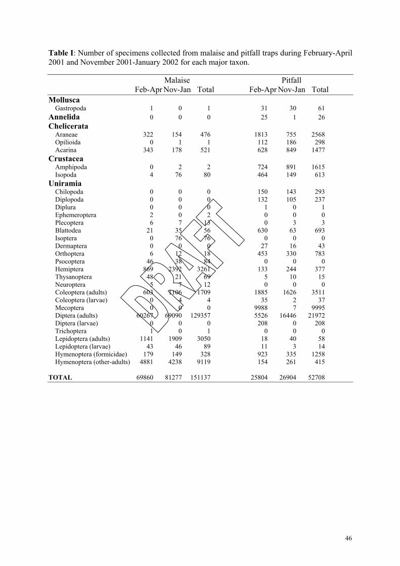
46

Table I: Number of specimens collected from malaise and pitfall traps during February-April2001 and November 2001-January 2002 for each major taxon.

Malaise PitfallFeb-Apr Nov-Jan Total Feb-Apr Nov-Jan Total

Mollusca Gastropoda 1 0 1 31 30 61Annelida 0 0 0 25 1 26Chelicerata Araneae 322 154 476 1813 755 2568 Opilioida 0 1 1 112 186 298 Acarina 343 178 521 628 849 1477Crustacea Amphipoda 0 2 2 724 891 1615 Isopoda 4 76 80 464 149 613Uniramia Chilopoda 0 0 0 150 143 293 Diplopoda 0 0 0 132 105 237 Diplura 0 0 0 1 0 1 Ephemeroptera 2 0 2 0 0 0 Plecoptera 6 7 13 0 3 3 Blattodea 21 35 56 630 63 693 Isoptera 0 76 76 0 0 0 Dermaptera 0 0 0 27 16 43 Orthoptera 6 12 18 453 330 783 Psocoptera 46 38 84 0 0 0 Hemiptera 869 2392 3261 133 244 377 Thysanoptera 48 21 69 5 10 15 Neuroptera 5 7 12 0 0 0 Coleoptera (adults) 603 1106 1709 1885 1626 3511 Coleoptera (larvae) 0 4 4 35 2 37 Mecoptera 0 0 0 9988 7 9995 Diptera (adults) 60267 69090 129357 5526 16446 21972 Diptera (larvae) 0 0 0 208 0 208 Trichoptera 1 0 1 0 0 0 Lepidoptera (adults) 1141 1909 3050 18 40 58 Lepidoptera (larvae) 43 46 89 11 3 14 Hymenoptera (formicidae) 179 149 328 923 335 1258 Hymenoptera (other-adults) 4881 4238 9119 154 261 415

TOTAL 69860 81277 151137 25804 26904 52708

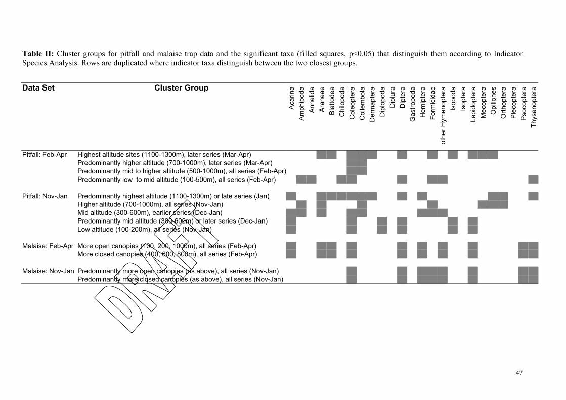
47

Table II: Cluster groups for pitfall and malaise trap data and the significant taxa (filled squares, p<0.05) that distinguish them according to IndicatorSpecies Analysis. Rows are duplicated where indicator taxa distinguish between the two closest groups.

Data Set Cluster Group

Acar

ina

Amph

ipod

aAn

nelid

aAr

anea

eBl

atto

dea

Chi

lopo

daC

oleo

pter

aC

olle

mbo

laD

erm

apte

raD

iplo

poda

Dip

lura

Dip

tera

Gas

tropo

daH

emip

tera

Form

icid

aeot

her H

ymen

opte

raIs

opod

aIs

opte

raLe

pido

pter

aM

ecop

tera

Opi

lione

sO

rthop

tera

Plec

opte

raPs

ocop

tera

Thys

anop

tera

Pitfall: Feb-Apr Highest altitude sites (1100-1300m), later series (Mar-Apr)Predominantly higher altitude (700-1000m), later series (Mar-Apr)Predominantly mid to higher altitude (500-1000m), all series (Feb-Apr)Predominantly low to mid altitude (100-500m), all series (Feb-Apr)

Pitfall: Nov-Jan Predominantly highest altitude (1100-1300m) or late series (Jan)Higher altitude (700-1000m), all series (Nov-Jan)Mid altitude (300-600m), earlier series (Dec-Jan)Predominantly mid altitude (300-600m) or later series (Dec-Jan)Low altitude (100-200m), all series (Nov-Jan)

Malaise: Feb-Apr More open canopies (100, 200, 1000m), all series (Feb-Apr)More closed canopies (400, 600, 800m), all series (Feb-Apr)

Malaise: Nov-Jan Predominantly more open canopies (as above), all series (Nov-Jan)Predominantly more closed canopies (as above), all series (Nov-Jan)

Doran et al. Change in vegetation and invertebrate altitudinal assemblages.

48

FIGURE CAPTIONS

Figure 1: Altitudinal transects at Mt Weld and the Warra LTER site.NOTE FOR EDITOR: although this .pdf file has colour elements it has been produced forreproduction in black and white or grayscale. There is no need to reproduce it in colour.

Figure 2: Total and mean vascular plant species richness for all plots on all transects, plottedagainst altitude. The percentage importance value (IV) of rainforest species is shown as anindication of disturbance history (high percentage scores of rainforest are likely to have had alower fire frequency.

Figure 3: Graph of the altitude gradient in classes of 100 m units showing for each altitudeclass a) Jaccard’s percentage dissimilarity score for adjacent altitude classes; b) Thepercentage of the species reaching a limit (upper or lower) c) The percentage of speciesreaching their lower altitude limit; d) The percentage of species reaching their upper altitudelimit; e) The interpolated species richness class; and f) the actual species richness.

Figure 4: Joint plot of the MDS ordination of plant species importance values (IV) dataoverlain with the significant (P<0.05) environmental and vegetation attribute variables. Figure4a (above) shows the ordination of plots from transect A and D. Figure 4b (below) shows theordination of all lowland forest plots (transects A, B C and D) below 800 m in altitude.

Figure 5: Ordination pattern emerging for the pitfall trap data over February-April, includinghigh altitude data. Stress = 0.099. Figure 5a (above) with environmental vectors overlaid.Figure 5b (below) with significant taxon vectors overlaid. Note: D06 (series 3) was excludedas an extreme outlier.

Figure 6: Cluster groups emerging for pitfall trap data (high altitude sites excluded, with sitelabels as per text). • Figure 6a (above) is for February-April. Group 1 consists of low altitude sites for all

months, Group 2 consists of mid altitude sites for all months and higher altitude sites forFebruary, while Group 3 consists predominantly of the higher altitude sites for March andApril.

• Figure 6b (below) is for November-January. Group 1 consists of low altitude sites, Group2 consists of lower to mid altitude sites for January, Group 3 consists of lower to midaltitude sites for November and December, while group 4 consists of higher altitude sitesfor all months.

Figure 7: Ordination pattern emerging for the malaise trap data over February-April. Stress =0.050. Figure 7a (above) with environmental vectors overlaid. Figure 7b (below) withsignificant taxon vectors overlaid. Site labels as per text (‘m’ denotes malaise).

Figure 8: Cluster groups emerging for malaise trap data (site labels as per text, ‘m’ denotesmalaise). • Figure 8a (above) is for February-April. Group 1 consists of all 400, 600 and 800m

samples, while group 2 consists of all 100, 200 and 1000m samples.• Figure 8b (below) is for November-January. Group 1 again consists of nearly all 400, 600

and 800m samples, while group 2 consists of predominantly all 100, 200 and 1000msamples.

Doran et al. Change in vegetation and invertebrate altitudinal assemblages.

49

Figure 1 in electronic supplement: Total vascular plant species richness in 0.1 ha plotsgraphed against the percentage importance value of rainforest species (IVRF). (Total speciesrichness = 29.9 +1.2 x IVRF – 0.025 x IVRF squared).

Figure 2 in electronic supplement: Total vascular plant species richness in 0.1 ha plotsgraphed against altitude with a polynomial regression model fitted against the data. (Totalspecies richness = 18.3 – 0.01 x altitude + 0.00001 x altitude squared).

Figure 3 in electronic supplement: Mean vascular plant species richness in 10 by 0.01 hasubplots graphed against the altitude gradient with a polynomial regression model fittedagainst the data. ( Mean species richness = 18.1525 – 0.01028 x altitude + 0.0000125 xaltitude squared ).

Figure 4 in electronic supplement: Species richness (0.1 ha plots) of four plant life forms:Trees, Ferns, Herbs, and Woody non-trees (climbers and shrubs) graphed against thealtitudinal gradient.

Figure 5 in electronic supplement: Plot of dissimilarity scores for each pair of altitudinalclasses. Figure 5a (above) shows dissimilarity scores for each altitude class between 100 and700 m and all other altitudes. Figure 5b (below) shows dissimilarity scores for each altitudebetween 800 and 1300 m and all other altitudes.

Doran et al. Change in vegetation and invertebrate altitudinal assemblages.

50

Figure 1: See attached .PDF file/map “Figure 1_Doran.pdf”. NOTE FOR EDITOR: although this .pdf file has colour elements it has been produced forreproduction in black and white or grayscale. There is no need to reproduce it in colour.

Figure 2: Total and mean vascular plant species richness for all plots on all transects, plottedagainst altitude. The percentage importance value (IV) of rainforest species is shown as anindication of disturbance history (high percentage scores of rainforest are likely to have had alower fire frequency.

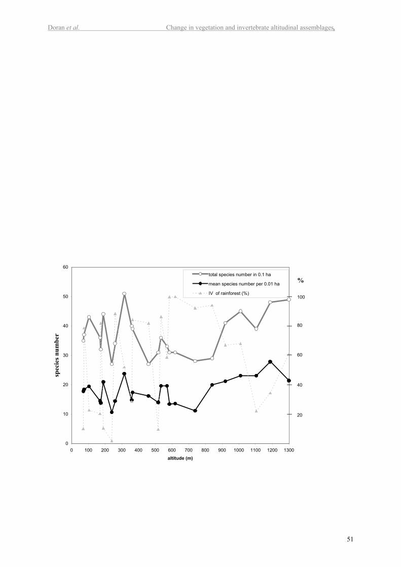
Doran et al. Change in vegetation and invertebrate altitudinal assemblages.

51

0

10

20

30

40

50

60

0 100 200 300 400 500 600 700 800 900 1000 1100 1200 1300

altitude (m)

spec

ies n

umbe

r

total species number in 0.1 ha

mean species number per 0.01 ha

IV of rainforest (%)100

80

60

40

20

%

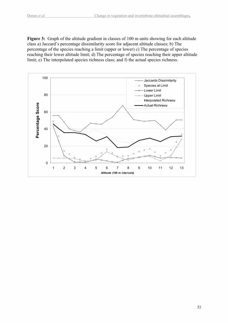
Doran et al. Change in vegetation and invertebrate altitudinal assemblages.

52

Figure 3: Graph of the altitude gradient in classes of 100 m units showing for each altitudeclass a) Jaccard’s percentage dissimilarity score for adjacent altitude classes; b) Thepercentage of the species reaching a limit (upper or lower) c) The percentage of speciesreaching their lower altitude limit; d) The percentage of species reaching their upper altitudelimit; e) The interpolated species richness class; and f) the actual species richness.

0

20

40

60

80

100

1 2 3 4 5 6 7 8 9 10 11 12 13Altitude (100 m intervals)

Perc

enta

ge S

core

Jaccards DissimilaritySpecies at LimitLower LimitUpper LimitInterpolated RichnessActual Richness

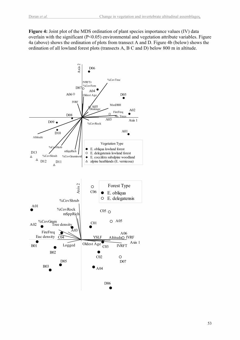
Doran et al. Change in vegetation and invertebrate altitudinal assemblages.

53

Figure 4: Joint plot of the MDS ordination of plant species importance values (IV) dataoverlain with the significant (P<0.05) environmental and vegetation attribute variables. Figure4a (above) shows the ordination of plots from transect A and D. Figure 4b (below) shows theordination of all lowland forest plots (transects A, B C and D) below 800 m in altitude.

A01

A02

A03

A04

A05

A06 D05

D06

D07

D08

D09

D10

D11D12

D13

IVRFTr

Altitude

%CovRock

Drainage

No. Trees

mSppRich

%CovTree

%CovShrub %CovGraminoid

%CovHerb

%CovFern

FireFreq

MaxDBH

Oldest Age

IVRF

Axis 1

Axi

s 2

Vegetation TypeE. obliqua lowland forestE. delegatensis lowland forestE. coccifera subalpine woodlandalpine heathlands (E. vernicosa)

B01

B02

B03

C01

C02

C03

C04

C05

C06

A01

A02A03

A04

A05

A06

D05

D06

D07

IVRFT

Altitude

%CovRock

Logged

Tree density

mSppRich

%CovShrub

%CovGram

FireFreqEuc density

Oldest Age

YSLF IVRFAxis 1

Axi

s 2 Forest TypeE. obliquaE. delegatensis

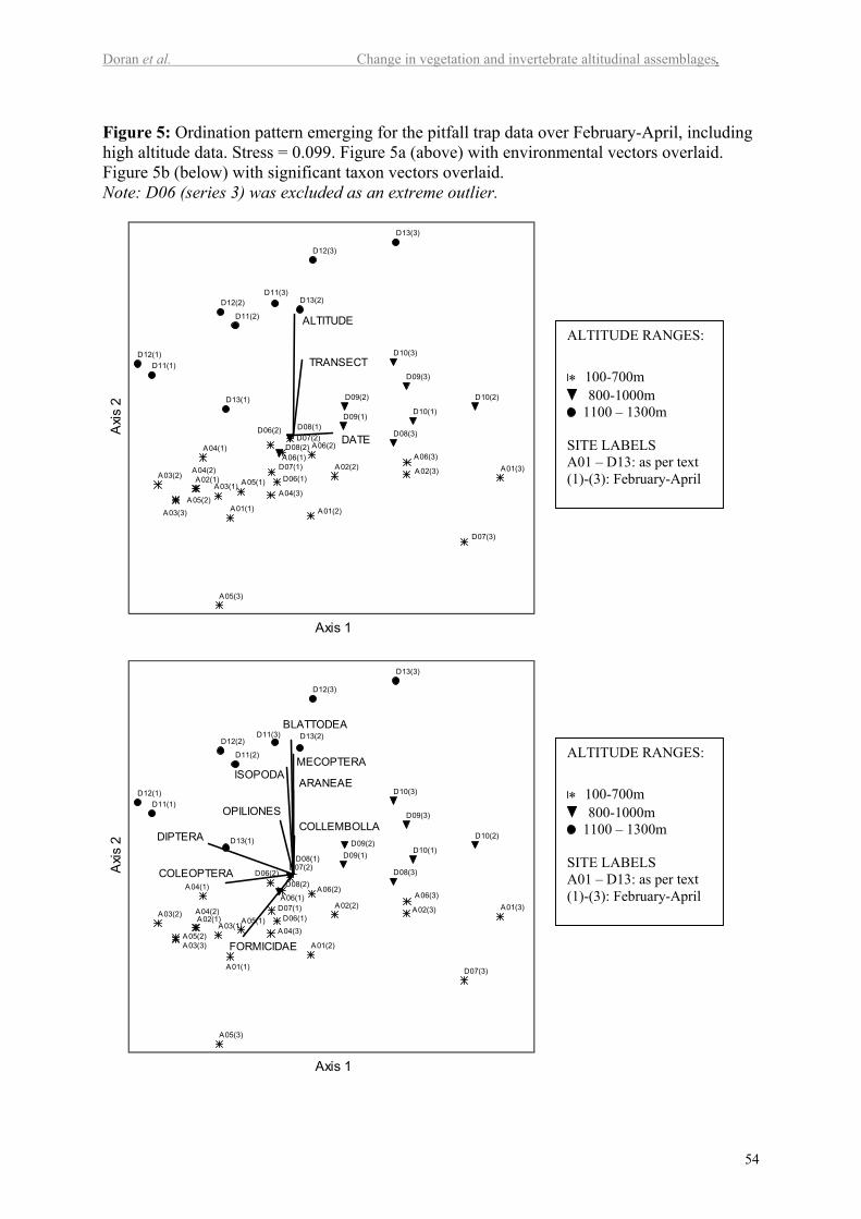
Doran et al. Change in vegetation and invertebrate altitudinal assemblages.

Figure 5: Ordination pattern emerging for the pitfall trap data over February-April, includinghigh altitude data. Stress = 0.099. Figure 5a (above) with environmental vectors overlaid.Figure 5b (below) with significant taxon vectors overlaid.Note: D06 (series 3) was excluded as an extreme outlier.

A01(1)

A02(1)A03(1)

A04(1)

A05(1)

A06(1)

D06(1)D07(1)

D08(1)D09(1) D10(1)

D11(1)D12(1)

D13(1)

A01(2)

A02(2)A03(2) A04(2)

A05(2)

A06(2)

D06(2)D07(2)

D08(2)

D09(2) D10(2)

D11(2)

D12(2) D13(2)

A02(3)

A03(3)

A04(3)

A05(3)

A06(3)

D07(

D08(3)

D09(3)

D10(3)

D11(3)

D12(3)

D13(3)

ALTITUDE

TRANSECT

DATE

Axis 1

Axis

2

A01(1)

A02(1)A03(1)

A04(1)

A05(1)

A06(1)

D06(1)D07(1)

D08(1) D09(1) D10(1)

D11(1)D12(1)

D13(1)

A01(2)

A02(2)A03(2) A04(2)

A05(2)

A06(2)

D06(2)D07(2)

D08(2)

D09(2)

D11(2)

D12(2) D13(2)

A02(3)

A03(3)

A04(3)

A05(3)

A06(3)

D07(3)

D08(3)

D09(3)

D10(3)

D11(3)

D12(3)

D13(3)

ARANEAE

BLATTODEA

COLEOPTERA

COLLEMBOLLADIPTERA

FORMICIDAE

ISOPODAMECOPTERA

OPILIONES

Axis 1

Axis

2

ALTITUDE RANGES:

* 100-700m 800-1000m 1100 – 1300m

SITE LABELSA01 – D13: as per text(1)-(3): February-April

A01(3)

3)

ALTITUDE RANGES:

* 100-700m 800-1000m 1100 – 1300m

D10(2)

54

A01(3)

SITE LABELSA01 – D13: as per text(1)-(3): February-April

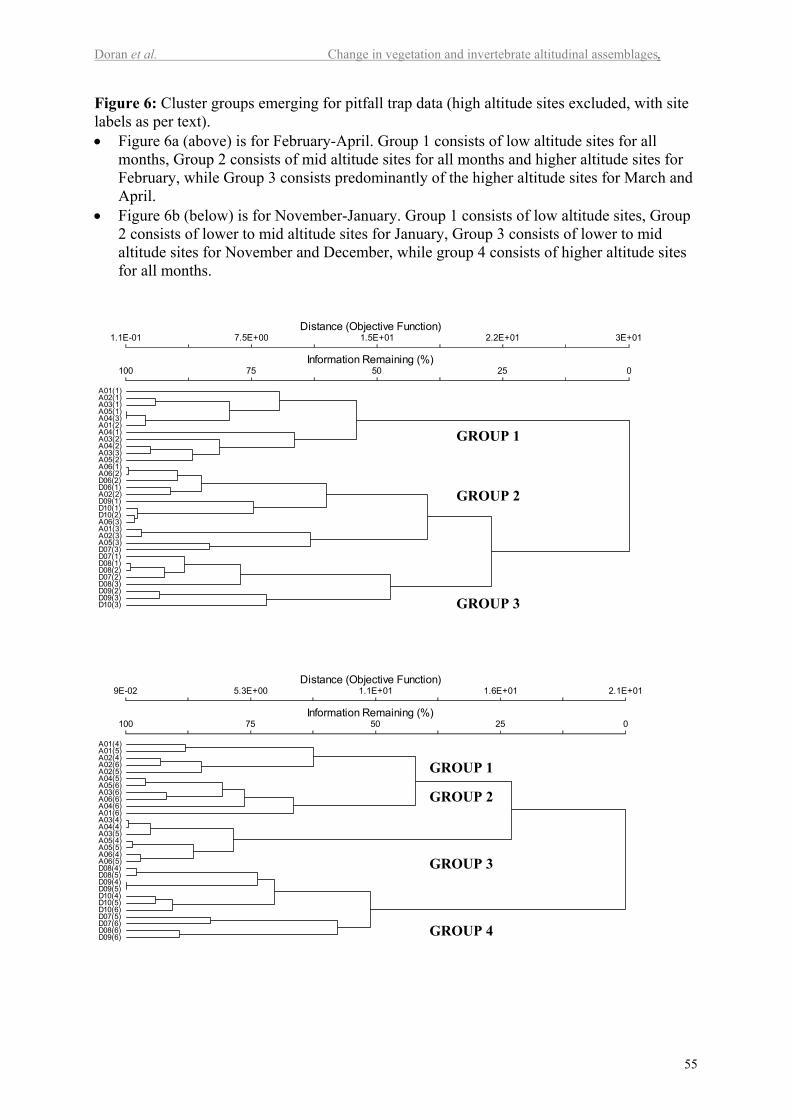
Doran et al. Change in vegetation and invertebrate altitudinal assemblages.

55

Figure 6: Cluster groups emerging for pitfall trap data (high altitude sites excluded, with sitelabels as per text). • Figure 6a (above) is for February-April. Group 1 consists of low altitude sites for all

months, Group 2 consists of mid altitude sites for all months and higher altitude sites forFebruary, while Group 3 consists predominantly of the higher altitude sites for March andApril.

• Figure 6b (below) is for November-January. Group 1 consists of low altitude sites, Group2 consists of lower to mid altitude sites for January, Group 3 consists of lower to midaltitude sites for November and December, while group 4 consists of higher altitude sitesfor all months.

Distance (Objective Function)

Information Remaining (%)

1.1E-01

100

7.5E+00

75

1.5E+01

50

2.2E+01

25

3E+01

0

A01(1)A02(1)A03(1)A05(1)A04(3)A01(2)A04(1)A03(2)A04(2)A03(3)A05(2)A06(1)A06(2)D06(2)D06(1)A02(2)D09(1)D10(1)D10(2)A06(3)A01(3)A02(3)A05(3)D07(3)D07(1)D08(1)D08(2)D07(2)D08(3)D09(2)D09(3)D10(3)

Distance (Objective Function)

Information Remaining (%)

9E-02

100

5.3E+00

75

1.1E+01

50

1.6E+01

25

2.1E+01

0

A01(4)A01(5)A02(4)A02(6)A02(5)A04(5)A05(6)A03(6)A06(6)A04(6)A01(6)A03(4)A04(4)A03(5)A05(4)A05(5)A06(4)A06(5)D08(4)D08(5)D09(4)D09(5)D10(4)D10(5)D10(6)D07(5)D07(6)D08(6)D09(6)

GROUP 1

GROUP 2

GROUP 3

GROUP 1

GROUP 2

GROUP 3

GROUP 4

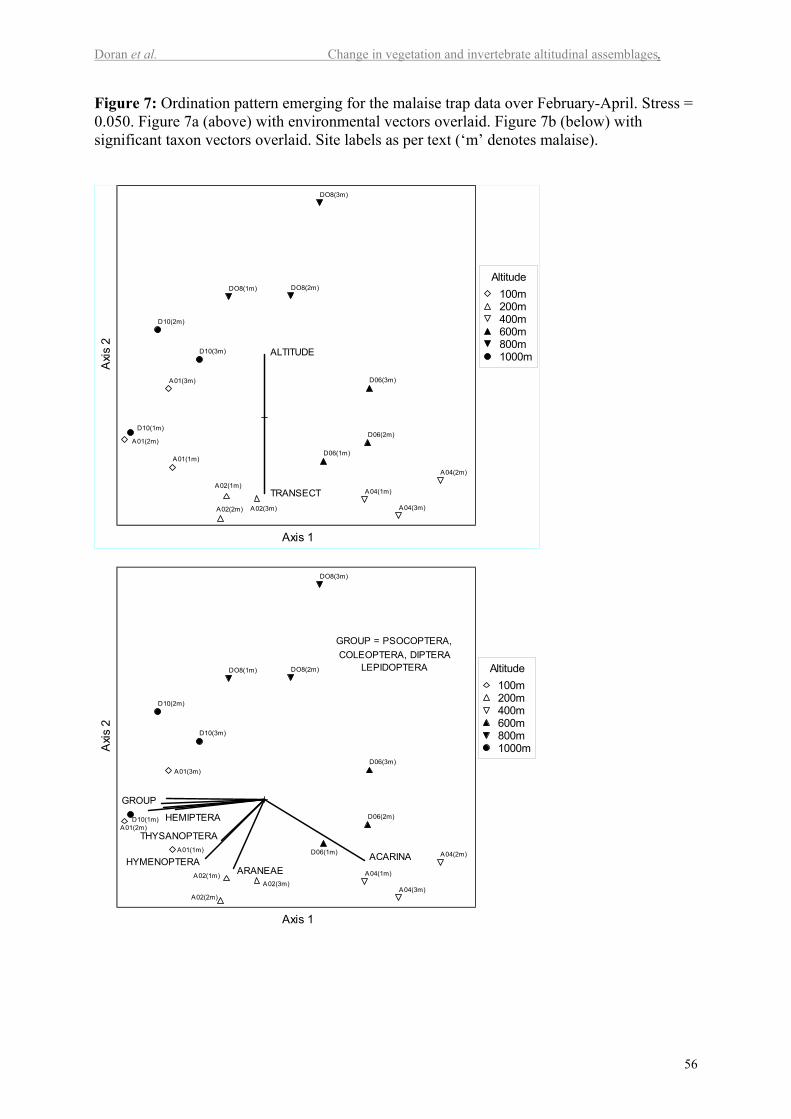
Doran et al. Change in vegetation and invertebrate altitudinal assemblages.

56

Figure 7: Ordination pattern emerging for the malaise trap data over February-April. Stress =0.050. Figure 7a (above) with environmental vectors overlaid. Figure 7b (below) withsignificant taxon vectors overlaid. Site labels as per text (‘m’ denotes malaise).

D06(1m)

DO8(1m)

D10(1m)

A01(1m)

A02(1m)A04(1m)

D06(2m)

DO8(2m)

D10(2m)

A01(2m)

A02(2m)

A04(2m)

D06(3m)

DO8(3m)

D10(3m)

A01(3m)

A02(3m) A04(3m)

ALTITUDE

TRANSECT

Axis 1

Axi

s 2

Altitude100m200m400m600m800m1000m

D06(1m)

DO8(1m)

D10(1m)

A01(1m)

A02(1m) A04(1m)

D06(2m)

DO8(2m)

D10(2m)

A01(2m)

A02(2m)

A04(2m)

D06(3m)

DO8(3m)

D10(3m)

A01(3m)

A02(3m)A04(3m)

ACARINAARANEAE

COLEOPTERA, DIPTERA

GROUP

HEMIPTERA

HYMENOPTERA

LEPIDOPTERA

GROUP = PSOCOPTERA,

THYSANOPTERA

Axis 1

Axi

s 2

Altitude100m200m400m600m800m1000m

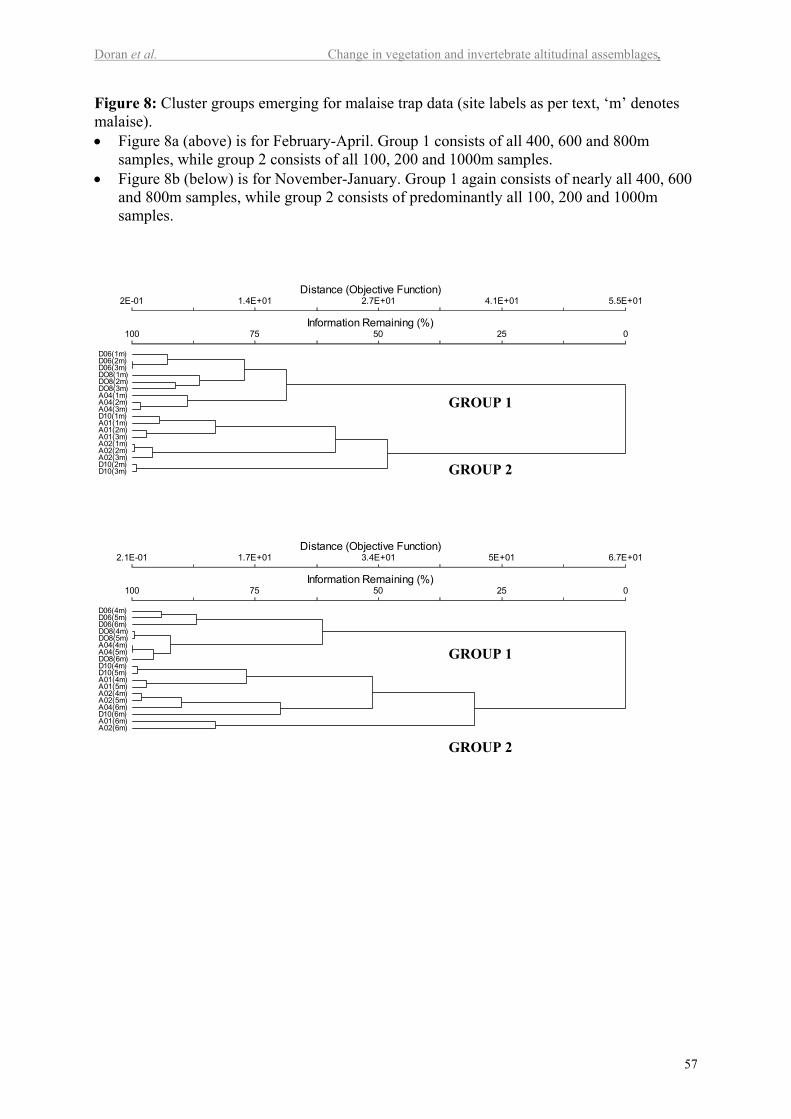
Doran et al. Change in vegetation and invertebrate altitudinal assemblages.

57

Figure 8: Cluster groups emerging for malaise trap data (site labels as per text, ‘m’ denotesmalaise). • Figure 8a (above) is for February-April. Group 1 consists of all 400, 600 and 800m

samples, while group 2 consists of all 100, 200 and 1000m samples.• Figure 8b (below) is for November-January. Group 1 again consists of nearly all 400, 600

and 800m samples, while group 2 consists of predominantly all 100, 200 and 1000msamples.

Distance (Objective Function)

Information Remaining (%)

2E-01

100

1.4E+01

75

2.7E+01

50

4.1E+01

25

5.5E+01

0

D06(1m)D06(2m)D06(3m)DO8(1m)DO8(2m)DO8(3m)A04(1m)A04(2m)A04(3m)D10(1m)A01(1m)A01(2m)A01(3m)A02(1m)A02(2m)A02(3m)D10(2m)D10(3m)

Distance (Objective Function)

Information Remaining (%)

2.1E-01

100

1.7E+01

75

3.4E+01

50

5E+01

25

6.7E+01

0

D06(4m)D06(5m)D06(6m)DO8(4m)DO8(5m)A04(4m)A04(5m)DO8(6m)D10(4m)D10(5m)A01(4m)A01(5m)A02(4m)A02(5m)A04(6m)D10(6m)A01(6m)A02(6m)

GROUP 1

GROUP 2

GROUP 1

GROUP 2

Doran et al. Change in vegetation and invertebrate altitudinal assemblages.

58

THE FOLLOWING PAGES CONTAINTABLES AND FIGURES

FOR THE ELECTRONIC SUPPLEMENT

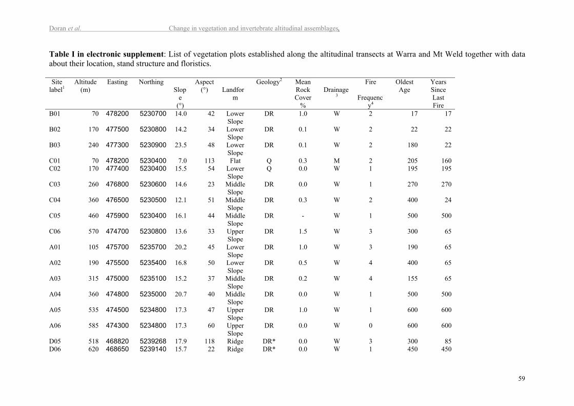
Doran et al. Change in vegetation and invertebrate altitudinal assemblages.

59

Table I in electronic supplement: List of vegetation plots established along the altitudinal transects at Warra and Mt Weld together with dataabout their location, stand structure and floristics.

Sitelabel1

Altitude(m)

Easting NorthingSlop

e(°)

Aspect(°) Landfor

m

Geology2 MeanRockCover

%

Drainage3

Fire

Frequency4

OldestAge

YearsSinceLastFire

B01 70 478200 5230700 14.0 42 LowerSlope

DR 1.0 W 2 17 17

B02 170 477500 5230800 14.2 34 LowerSlope

DR 0.1 W 2 22 22

B03 240 477300 5230900 23.5 48 LowerSlope

DR 0.1 W 2 180 22

C01 70 478200 5230400 7.0 113 Flat Q 0.3 M 2 205 160C02 170 477400 5230400 15.5 54 Lower

SlopeQ 0.0 W 1 195 195

C03 260 476800 5230600 14.6 23 MiddleSlope

DR 0.0 W 1 270 270

C04 360 476500 5230500 12.1 51 MiddleSlope

DR 0.3 W 2 400 24

C05 460 475900 5230400 16.1 44 MiddleSlope

DR - W 1 500 500

C06 570 474700 5230800 13.6 33 UpperSlope

DR 1.5 W 3 300 65

A01 105 475700 5235700 20.2 45 LowerSlope

DR 1.0 W 3 190 65

A02 190 475500 5235400 16.8 50 LowerSlope

DR 0.5 W 4 400 65

A03 315 475000 5235100 15.2 37 MiddleSlope

DR 0.2 W 4 155 65

A04 360 474800 5235000 20.7 40 MiddleSlope

DR 0.0 W 1 500 500

A05 535 474500 5234800 17.3 47 UpperSlope

DR 1.0 W 1 600 600

A06 585 474300 5234800 17.3 60 UpperSlope

DR 0.0 W 0 600 600

D05 518 468820 5239268 17.9 118 Ridge DR* 0.0 W 3 300 85D06 620 468650 5239140 15.7 22 Ridge DR* 0.0 W 1 450 450

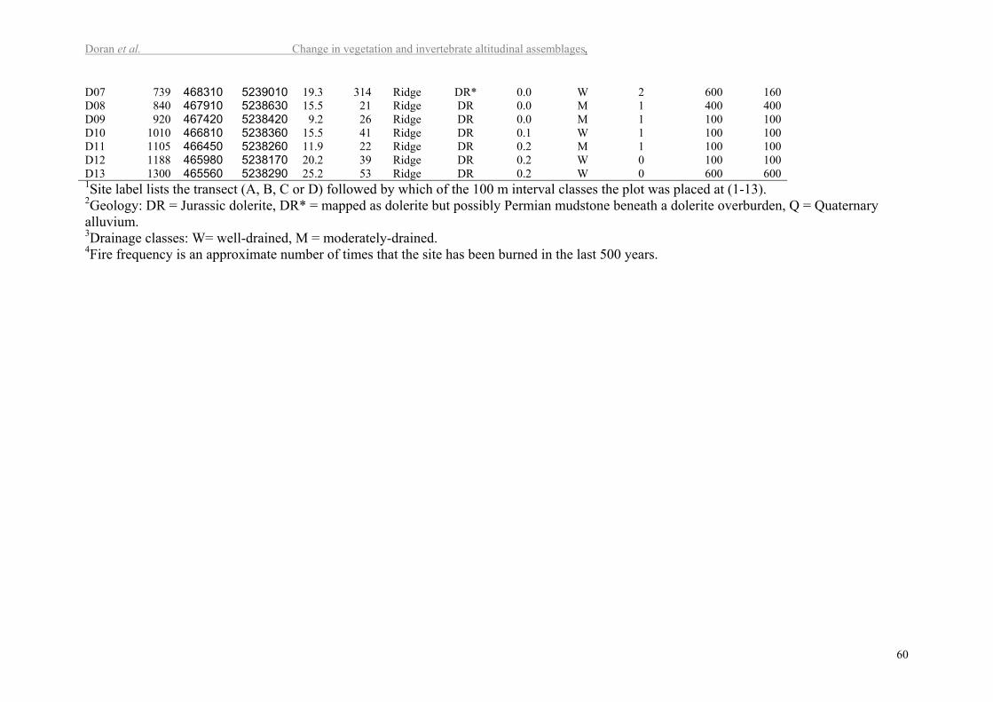
Doran et al. Change in vegetation and invertebrate altitudinal assemblages.

60

D07 739 468310 5239010 19.3 314 Ridge DR* 0.0 W 2 600 160D08 840 467910 5238630 15.5 21 Ridge DR 0.0 M 1 400 400D09 920 467420 5238420 9.2 26 Ridge DR 0.0 M 1 100 100D10 1010 466810 5238360 15.5 41 Ridge DR 0.1 W 1 100 100D11 1105 466450 5238260 11.9 22 Ridge DR 0.2 M 1 100 100D12 1188 465980 5238170 20.2 39 Ridge DR 0.2 W 0 100 100D13 1300 465560 5238290 25.2 53 Ridge DR 0.2 W 0 600 6001Site label lists the transect (A, B, C or D) followed by which of the 100 m interval classes the plot was placed at (1-13).2Geology: DR = Jurassic dolerite, DR* = mapped as dolerite but possibly Permian mudstone beneath a dolerite overburden, Q = Quaternaryalluvium.3Drainage classes: W= well-drained, M = moderately-drained.4Fire frequency is an approximate number of times that the site has been burned in the last 500 years.

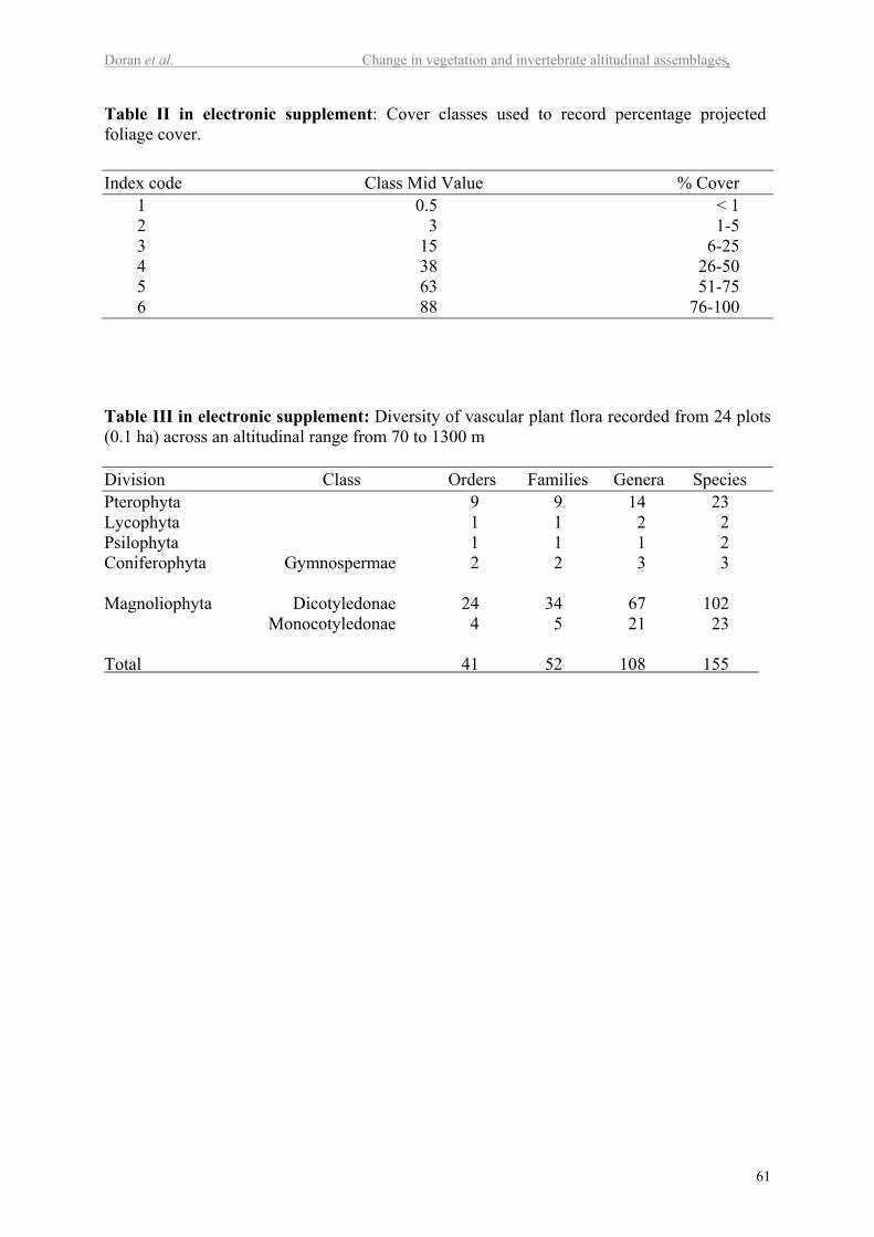
Doran et al. Change in vegetation and invertebrate altitudinal assemblages.

61

Table II in electronic supplement: Cover classes used to record percentage projectedfoliage cover.

Index code Class Mid Value % Cover1 0.5 < 12 3 1-53 15 6-254 38 26-505 63 51-756 88 76-100

Table III in electronic supplement: Diversity of vascular plant flora recorded from 24 plots(0.1 ha) across an altitudinal range from 70 to 1300 m

Division Class Orders Families Genera SpeciesPterophyta 9 9 14 23Lycophyta 1 1 2 2Psilophyta 1 1 1 2Coniferophyta Gymnospermae 2 2 3 3

Magnoliophyta Dicotyledonae 24 34 67 102Monocotyledonae 4 5 21 23

Total 41 52 108 155

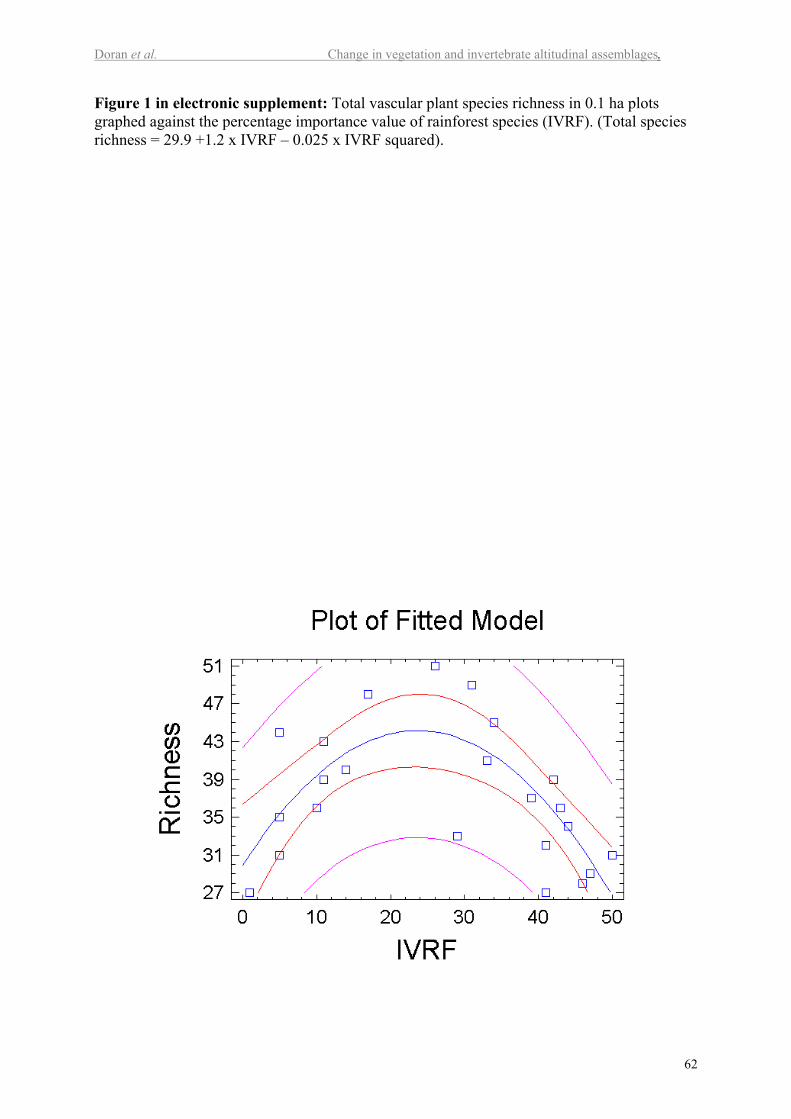
Doran et al. Change in vegetation and invertebrate altitudinal assemblages.

62

Figure 1 in electronic supplement: Total vascular plant species richness in 0.1 ha plotsgraphed against the percentage importance value of rainforest species (IVRF). (Total speciesrichness = 29.9 +1.2 x IVRF – 0.025 x IVRF squared).

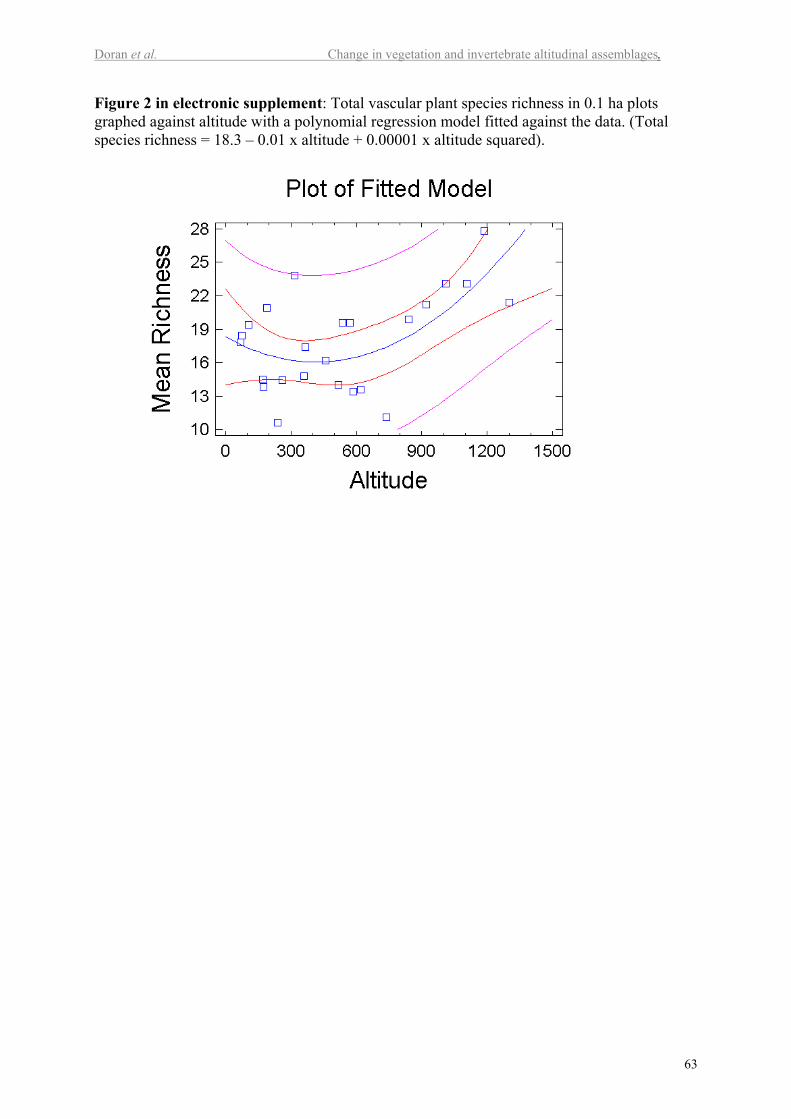
Doran et al. Change in vegetation and invertebrate altitudinal assemblages.

63

Figure 2 in electronic supplement: Total vascular plant species richness in 0.1 ha plotsgraphed against altitude with a polynomial regression model fitted against the data. (Totalspecies richness = 18.3 – 0.01 x altitude + 0.00001 x altitude squared).

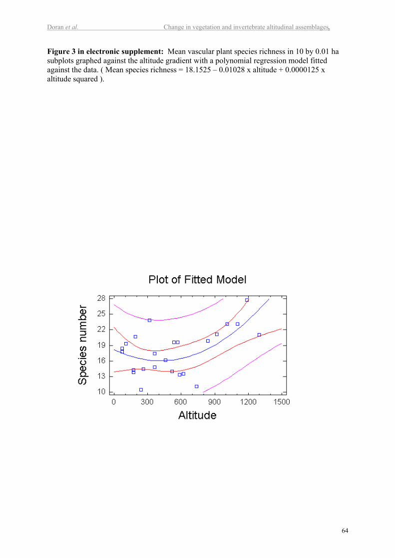
Doran et al. Change in vegetation and invertebrate altitudinal assemblages.

64

Figure 3 in electronic supplement: Mean vascular plant species richness in 10 by 0.01 hasubplots graphed against the altitude gradient with a polynomial regression model fittedagainst the data. ( Mean species richness = 18.1525 – 0.01028 x altitude + 0.0000125 xaltitude squared ).

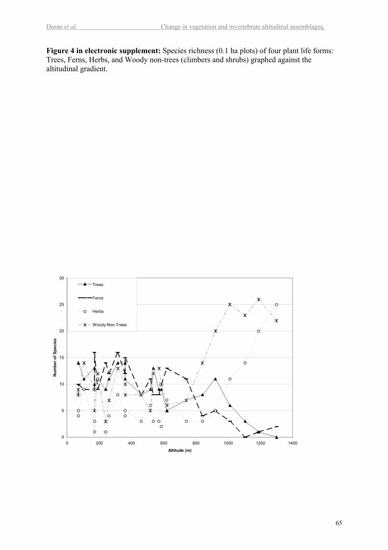
Doran et al. Change in vegetation and invertebrate altitudinal assemblages.

65

Figure 4 in electronic supplement: Species richness (0.1 ha plots) of four plant life forms:Trees, Ferns, Herbs, and Woody non-trees (climbers and shrubs) graphed against thealtitudinal gradient.

0

5

10

15

20

25

30

0 200 400 600 800 1000 1200 1400

Altitude (m)

Num

ber o

f Spe

cies

Trees

Ferns

Herbs

Woody Non-Trees

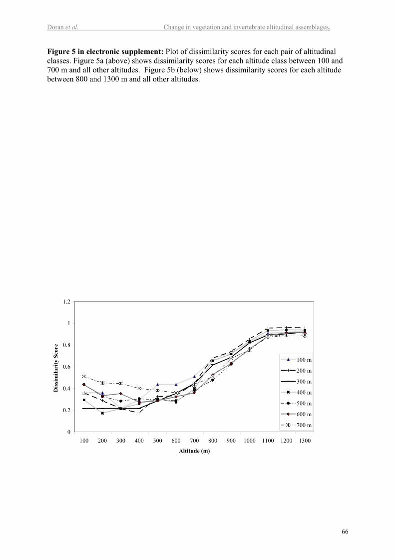
Doran et al. Change in vegetation and invertebrate altitudinal assemblages.

66

Figure 5 in electronic supplement: Plot of dissimilarity scores for each pair of altitudinalclasses. Figure 5a (above) shows dissimilarity scores for each altitude class between 100 and700 m and all other altitudes. Figure 5b (below) shows dissimilarity scores for each altitudebetween 800 and 1300 m and all other altitudes.

0

0.2

0.4

0.6

0.8

1

1.2

100 200 300 400 500 600 700 800 900 1000 1100 1200 1300

Altitude (m)

Dis

sim

ilari

ty S

core

100 m

200 m

300 m

400 m

500 m

600 m

700 m

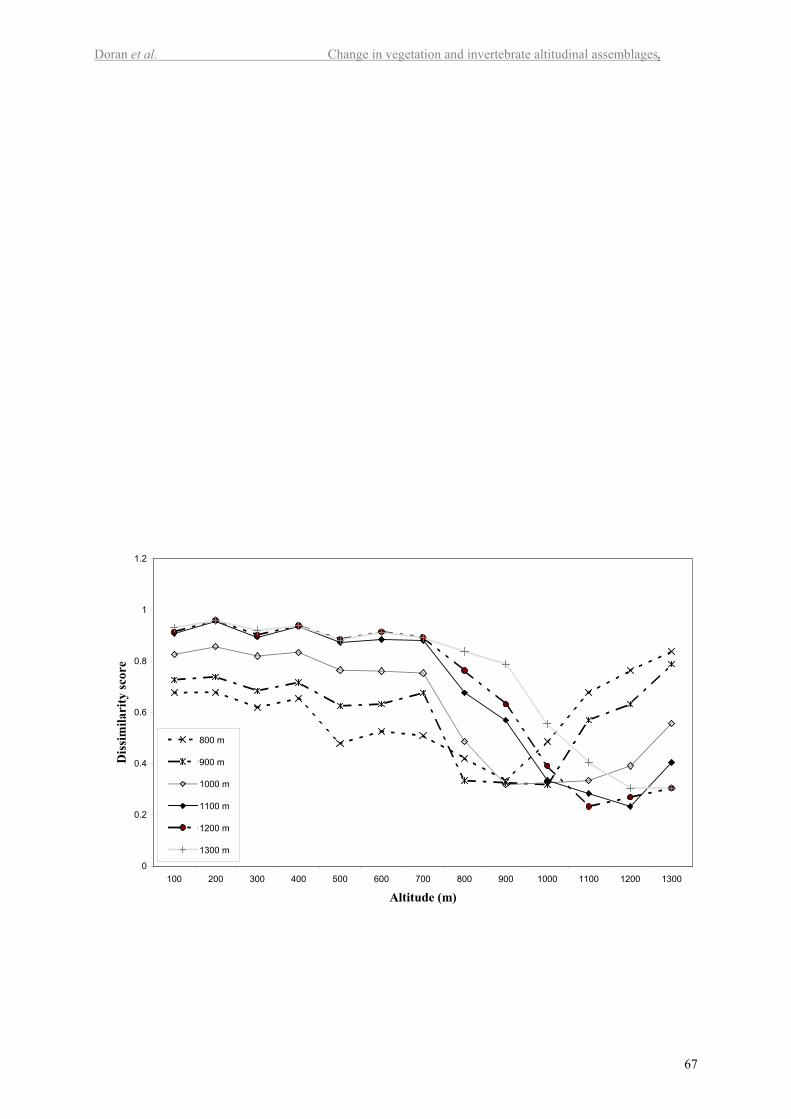
Doran et al. Change in vegetation and invertebrate altitudinal assemblages.

67

0

0.2

0.4

0.6

0.8

1

1.2

100 200 300 400 500 600 700 800 900 1000 1100 1200 1300

Altitude (m)

Dis

sim

ilari

ty sc

ore

800 m

900 m

1000 m

1100 m

1200 m

1300 m