Multicloud Convective Parametrizations with Crude Vertical Structure

Theor. Comput. Fluid Dyn. (2006) 20: 351–375DOI 10.1007/s00162-006-0013-2

ORIGINAL ARTICLE

Boualem Khouider · Andrew J. Majda

Multicloud convective parametrizations with crude verticalstructure

Received: 1 August 2005 / Accepted: 31 January 2006 / Published online: 5 May 2006© Springer-Verlag 2006

Abstract Recent observational analysis reveals the central role of three multi-cloud types, congestus, strati-form, and deep convective cumulus clouds, in the dynamics of large scale convectively coupled Kelvin waves,westward propagating two-day waves, and the Madden–Julian oscillation. The authors have recently developeda systematic model convective parametrization highlighting the dynamic role of the three cloud types throughtwo baroclinic modes of vertical structure: a deep convective heating mode and a second mode with low levelheating and cooling corresponding respectively to congestus and stratiform clouds. The model includes asystematic moisture equation where the lower troposphere moisture increases through detrainment of shallowcumulus clouds, evaporation of stratiform rain, and moisture convergence and decreases through deep con-vective precipitation and a nonlinear switch which favors either deep or congestus convection depending onwhether the troposphere is moist or dry. Here several new facets of these multi-cloud models are discussedincluding all the relevant time scales in the models and the links with simpler parametrizations involving onlya single baroclinic mode in various limiting regimes. One of the new phenomena in the multi-cloud models isthe existence of suitable unstable radiative convective equilibria (RCE) involving a larger fraction of congestusclouds and a smaller fraction of deep convective clouds. Novel aspects of the linear and nonlinear stabilityof such unstable RCE’s are studied here. They include new modes of linear instability including mesoscalesecond baroclinic moist gravity waves, slow moving mesoscale modes resembling squall lines, and large scalestanding modes. The nonlinear instability of unstable RCE’s to homogeneous perturbations is studied withthree different types of nonlinear dynamics occurring which involve adjustment to a steady deep convectiveRCE, periodic oscillation, and even heteroclinic chaos in suitable parameter regimes.

Keywords Intermediate convective parametrizations · Multicloud models · Moist gravity waves · Tropicalconvection · Convective instability · Bifurcation · Periodic solutions · Heteroclinic orbits · Congestus clouds ·Stratiform clouds · Deep convective clouds

PACS 92.60, 92.60, 92.60, 02.30, 202.60

Communicated by R. Klein

B. Khouider(B)Mathematics and Statistics, University of Victoria,PO BOX 3045 STN CSC, Victoria, BC, Canada V8W 3P4E-mail: [email protected]

A. J. MajdaDepartment of Mathematics and Center for Atmosphere/Ocean Sciences,Courant Institute, New York University, 251 Mercer Street,New York, NY 10012, USA

352 B. Khouider, A. J. Majda

1 Introduction

Observational data indicate that tropical deep convection is organized on a hierarchy of scales ranging fromhundreds of kilometers due to mesoscale organized squall lines to intraseasonal oscillations over planetaryscales of order 40,000 km [1–3]. The present practical models for prediction of both weather and climateinvolve general circulation models (GCM) where the physical equations for these extremely complex flowsare discretized in space and time and the effects of unresolved processes are parametrized according to variousrecipes [4,5]. With the current generation of supercomputers, the smallest possible mesh spacings are roughly50–100 km for short-term tropical weather simulations and of 200–300 km for short-term climate simulations.With such coarse mesh spacing, despite much progress in the parametrization of tropical convection, the currentgeneration of GCMs [4,5] still fails to reproduce most of the significant features of the observational record[1–3] regarding tropical convection [4,5]. Thus, given the importance of the tropics for short-term climate,new strategies for parametrizing the unresolved effects of tropical convection are very important.

In particular, contemporary general circulation models (GCMs) often perform poorly in parameterizingand/or resolving the observed large scale features of organized tropical convection such as convectively cou-pled waves as well as their impact on the planetary scale tropical circulation [6,7]; the reasons for such poorperformance are not well understood.

Simplified models with crude vertical resolution, typically involving a single baroclinic vertical mode,have been used for theoretical and numerical studies of various strategies for parameterizing moist convectionand convectively coupled waves [8–16]. Two types of models have dominated the arena of tropical moistconvection: convergence-driven models and quasi-equilibrium models. Convergence models date back to thework of Charney and Eliassen [17], followed by Yamasaki [18], Hayashi [19], and Lindzen [20]. The conver-gence models, also called convective instability of second kind (CISK) models, sustain convection throughlarge reservoirs of convectively available potential energy (CAPE) driven by low-level convergence. Suchmodels exhibit extreme sensitivity to grid scale behavior and linearized stability analysis reveals the unde-sirable feature of catastrophic instability with increasingly larger growth rates on the smallest scales [12,13].In the quasi-equilibrium thinking, first introduced by Arakawa and Schubert [21], one assumes a large scalequasi-equilibrium state where CAPE is nearly constant and deep convection acts as an energy regulator inrestoring quickly the equilibrium by consuming any excess of CAPE. The triggering and the amplificationof convection in quasi-equilibrium models rely on boundary layer variables and surface fluxes. Indeed, suchquasi-equilibrium models are linearly [10] and even nonlinearly stable [16]. The most popular mechanismused in concert with the quasi-equilibrium models to create instability is wind induced surface heat exchange(WISHE) [8,22].

Recent analysis of observations over the warm pool in the tropics reveals the ubiquity of three cloud typesabove the boundary layer: shallow congestus clouds, stratiform clouds, and deep penetrative cumulus clouds[23,24]. Furthermore, recent analysis of convectively coupled waves on the large scales reveals a similarmulti-cloud convective structure with leading shallow congestus cloud decks which moisten and preconditionthe lower troposphere followed by deep convection and finally trailing decks of stratiform precipitation; thisstructure applies to the eastward propagating convectively coupled Kelvin waves [3,25] and westward prop-agating 2-day waves [26] which reside on equatorial synoptic scales of order 1,000–3,000 km in the lowertroposphere as well as the planetary scale Madden–Julian oscillation [27,28]. An inherently multi-scale theoryfor the Madden–Julian oscillation with qualitative agreement with observations which is based on these threecloud types has been developed recently [29,30]. While there is no doubt that WISHE plays an importantrole in hurricane development [31,32], there is no observational evidence directly linking the structure ofconvectively coupled Kelvin waves and 2-day waves to WISHE.

Besides providing intermediate models for parametrization of moist convection, detailed models withcrude vertical resolution are also important for explaining the observational record. Despite the observationalevidence, none of the models with a single vertical mode mentioned earlier account for the multi-mode natureof tropical convection and the importance of the different cloud types; shallow/congestus, stratiform and deep-penetrative cumulus clouds. They are concentrated solely on the deep-penetrative convection. Intermediatemodel parametrizations with two convective heating modes systematically representing, a deep-convectivemode and a stratiform mode, have first appeared in the work of Mapes [33]. Majda and Shefter [34] (hereafterMS) proposed a much simpler systematic version of Mapes’ model based on a Galerkin projection of theprimitive equations onto the first two linear-baroclinic modes yielding a set of two shallow water systems. Thefirst baroclinic system is heated by the deep convective clouds while the second baroclinic system is heatedaloft by the stratiform clouds. Linear stability analysis of this model convective parametrization revealed a

Multicloud convective parametrizations with crude vertical structure 353

mechanism of stratiform instability independent of WISHE [34,35]. Direct numerical simulations carried outin [35] revealed the resemblance of many features of the moist gravity waves for the MS model and the realworld convective superclusters as depicted in [35] and in observational papers (e.g. [25]). One visible short-coming of the MS model is however its short-cutting of the role of the shallow/congestus heating as in theearly Mapes’ model. Also, inherited from the quasi-equilibrium school [12,36], the Majda-Shefter model [34]uses very sensitive parameters which are nonphysically kept fixed/constant and spatially homogeneous, suchas the precipitation efficiency and the area fraction of deep convection.

Recently, the authors have developed a new multi-cloud model convective parametrization, within a frame-work similar to the MS model [34] involving crude vertical resolution with two vertical baroclinic modes [37].In addition to the deep convective and stratiform clouds, the present model carries cumulus congestus cloudswhich serve to heat the second baroclinic mode from below and cool it from above as in actual congestus clouddecks. The new model is based on a self-consistent derivation and it avoids many of the commonly used ad hocparameters. We systematically derived an equation for the vertically integrated water vapor with mean verticalbackground moisture profile forced by both the first baroclinic and second baroclinic (low-level) convergencewithin the physical constraints of conservation of vertically integrated moist static energy. Also the new modeltakes into account the dryness and moistness of the middle troposphere through a varying-inhomogeneousswitch parameter, �, in order to shut off or favor deep convection and to increase or decrease the downdraftsfrom the cooling associated with evaporation of shallow clouds and stratiform rain. Moreover, the congestusconvection is amplified whenever the middle troposphere is too dry to sustain deep convection and is shut offcompletely when deep-convection is at its maximum.

Linear stability analysis about a standard radiative convective equilibrium (RCE) solution performed in [37]revealed scale selective instability of convectively coupled gravity waves moving at 15–20 m/s at the planetaryand synoptic scales. The growth rates and the precise range of instability depend strongly on new features in themodel such as the strength of the lower tropospheric coupling of the deep convective parametrization, throughthe second baroclinic potential temperature and the second baroclinic moisture convergence. The heating andfluid dynamical fields of these moist gravity waves are similar to those encountered in the MS model whichare reminiscent of the moist Kelvin waves as observed, e.g. by Wheeler and Kiladis [3] and Straub and Kiladis[25], including their eastward propagation speed, the tilt in zonal wind and temperature, the upward motiondominating the heating region, the trailing stratiform part, etc. A notable new feature of the present models, alsopresent in observations, is congestus clouds leading to moistening of the lower troposphere as preconditioningfor deep convection. The budget analysis presented in [37] indicates that the basic instability operating in thenew multi-cloud models without WISHE is completely different from the stratiform instability of Majda andShefter [34].

Numerical simulations of the new multi-cloud parametrizations [38,39] reveal an important role for non-linear switches in the model with chaotic intermittent and turbulent regimes of nonlinear dynamics exhibitinglarge scale organization of convectively coupled waves which captures many features of the observationalrecord in a qualitative fashion.

The contents of the remainder of the paper are summarized next. In Sect. 2, the basic multi-cloud modelparametrization is reviewed. Section 3 shows the relationship between the present multi-cloud parametriza-tion with crude vertical resolution and other simpler model parametrizations in various limiting regimes. Theauthors briefly remarked in [37] that regimes of RCE with strong congestus clouds and little deep convection ina dry middle troposphere are linearly unstable to even homogeneous perturbations. Section 4 reviews the basicRCE solutions and develops the new phenomena that occur in this regime in detail including the nonlineardevelopment of homogeneous perturbations. The remarkable variety of new convectively coupled moisturewaves of linear instability are discussed in Sect. 5 while Sect. 6 summarizes the results presented herein andconcludes the paper. Finally, a detailed pedagogical derivation of the vertical average moisture equation utilizedin the multicloud parametrizations is given in the appendix at the end.

2 The multicloud model parametrization

2.1 The dynamical core

The dynamical core of the model convective parametrization proposed here consists of two coupled shallowwater systems. A direct heating mode forced by a bulk precipitation rate from deep penetrative clouds and asecond baroclinic mode forced by both stratiform heating and congestus heating.


∂v j

∂t+ U · ∇v j + βyv⊥

j − ∇θ j = −Cd(u0)v j − 1

τWv j

∂θ1

∂t+ U · ∇θ1 − div v1 = π

2√

2P + S1 (1)

∂θ2

∂t+ U · ∇θ2 − 1

4div v2 = π

2√

2(−Hs + Hc)+ S2.

The equations in (1) are obtained by a Galerkin projection of the hydrostatic primitive equations with constantbuoyancy frequency onto the first two baroclinic modes. More details of their derivation are found in [16,34,40].

In (1), v j = (u j , v j ) j=1,2 represent the first and second baroclinic velocities assuming G(z) = √2 cos

(π zHT

)

and G(2z) = √2 cos

(2π zHT

)vertical profiles, respectively, while θ j , j = 1, 2 are the corresponding potential

temperature components with the vertical profiles G ′(z) = √2 sin

(π zHT

)and 2G ′(2z) = 2

√2 sin

(2π zHT

),

respectively. Therefore, the total velocity field is approximated by

V ≈ U + G(z)v1 + G(2z)v2; w ≈ − HT

π

[G ′(z)div v1 + 1

2G ′(2z)divv2

]

where V is the horizontal velocity and w the vertical velocity. The total potential temperature is given approx-imately by

� ≈ z + G ′(z)θ1 + 2G ′(2z)θ2.

Here HT ≈ 16 km is the height of the tropical troposphere with 0 ≤ z ≤ HT and v⊥j = (−v j , u j )while U is the

incompressible barotropic wind which is set to zero hereafter, for the sake of simplicity. In (1), P ≥ 0 modelsthe heating from deep convection while Hs, Hc are the stratiform and congestus heating rates. Conceptually,the direct heating mode has a positive component and serves to heat the whole troposphere and is associatedwith a vertical shear flow. The second baroclinic mode is heated by the congestus clouds, Hc, from below andby the stratiform clouds, Hs, from above and therefore cooled by Hc from above and by Hs from below. It isassociated with a jet shear flow in the middle troposphere [34,35,37].

For simplicity, the nonlinear interactions between the first and second baroclinic modes are ignored butthey can be easily derived and incorporated into the equations [41–43]. The terms S1 and S2 are the radiativecooling rates associated with the first and second baroclinic modes respectively.

The system of equations in (1) is augmented by an equation for the boundary layer equivalent potentialtemperature, θeb, and another for the vertically integrated moisture content, q .

∂θeb

∂t= 1

hb(E − D)

∂q

∂t+ U · ∇q + div

((v1 + αv2)q

) + Q div(v1 + λv2) = −P + 1

HTD (2)

In (2), hb ≈ 500 m is the height of the moist boundary layer while Q, λ, and α are parameters associated witha prescribed moisture background and perturbation vertical profiles. According to the first equation in (2), θebchanges in response to the downdrafts, D, and the sea surface evaporation E . Here the term downdraft refersto the subsiding air resulting from evaporative cooling of congestus clouds and stratiform rain in the middleof the troposphere which therefore results in the moistening of the middle troposphere (increasing q) anddrying and cooling the boundary layer by bringing low θe from aloft. The troposphere moisture equation forq is derived from the bulk water vapor budget equation by imposing a moisture stratification-like backgroundvertical profile qv = Q(z) + q . We give a detailed pedagogical derivation of this equation in the Appendixstarting from the equations of bulk cloud microphysics both for its importance and to illustrate the systematicreduced modeling procedure. The approximate numerical values of λ = 0.8 and α = 0.1, follow directly fromthe derivation, while the coefficient Q arises from the background moisture gradient. We use the standardvalue Q ≈ 0.9 [16,36].

In full generality, the parametrizations in (1) and (2) automatically have conservation of an approxima-tion to vertically integrated moist static energy. Notice that, the precipitation rate in (2), balances the vertical


average of the total convective heating rate in (1), therefore leading to the conservation of the vertical averageof the equivalent potential temperature 〈θe〉 = 〈Q(z)〉 + q + 〈�〉 + hb

HTθeb when the external forces, namely,

the radiative cooling rates, S1, S2, and the evaporative heating, E , are set to zero. Also note that the sensibleheating flux has been ignored in (1) for simplicity since this is a relatively small contribution in the tropics.Here and elsewhere in the text 〈 f 〉 ≡ (1/HT)

∫ HT0 f (z) dz.

The equations in (1) and (2) for the prognostic variables q, θeb, θ j , v j , j = 1, 2, are written in non-dimen-sional units where the equatorial Rossby deformation radius, Le ≈ 1,500 km is the length scale, the firstbaroclinic dry gravity wave speed, c ≈ 50 m/s, is the velocity scale, T = Le/c ≈ 8 h is the associated

time scale, and the dry-static stratification α = HT N 2θ0πg ≈ 15 K is the temperature unit scale. The basic bulk

parameters of the model are listed in Table 1 for the reader’s convenience.

2.2 The convective parametrization

The surface evaporative heating, E , in (2) obeys an adjustment equation toward the boundary layer saturationequivalent potential temperature, θ∗

eb,

1

hbE = 1

τe(θ∗

eb − θeb) (3)

with τe is the evaporative time scale. The value of θ∗eb on a warm ocean surface is fixed such that at radiative

convective equilibrium (RCE) we have θ∗eb − θeb = 10 K, according to the Jordan sounding [44].

Besides the second baroclinic moisture advection in (2), the originality of the present model resides in a newtreatment of the deep convective heating/precipitation, P , and the downdrafts, D, as well as the introductionof the congestus heating, Hc, into the θ2 equation. The middle tropospheric equivalent potential temperatureanomaly is defined approximately by

θem ≈ q + 2√

2

π(θ1 + α2θ2) (4)

where α2 = 0.1. Notice that the coefficient 2√

2/π in (4) results from the vertical average of the first baroclinicpotential temperature,

√2θ1 sin(π z/HT), while the small value for α2 adds a non-zero contribution from θ2 to

θem to include its contribution from the lower middle troposphere although its vertical average is zero.Following [37], we use a switch parameter � which serves as a measure for the moistness and dryness of

the middle troposphere [31]. When the discrepancy between the boundary layer and the middle troposphereequivalent potential temperature is above some fixed threshold, θ+, the atmosphere is defined as dry. Moistparcels rising from the boundary layer will have their moisture quickly diluted by entrainment of dry air, hencelosing buoyancy and stop to convect. In this case, we set� = 1 which automatically inhibits deep convectionin the model (see below). When this discrepancy is below some lower value, θ−, we have a relatively moist

Table 1 Bulk constants in two layer mode model

HT = 16 km: height or the tropical troposphereQ = 0.9: moisture stratification factorλ = 0.8: 2n baroclinic relative contribution to the moisture convergence associated with the moisture backgroundα = 0.1: 2n baroclinic relative contribution to the moisture (nonlinear) convergence associated with the moisture anomaliesτW = 75 days: Rayleigh-wind friction relaxation timeτR = 50 days: Newtonian cooling relaxation timecd = 0.001: boundary layer turbulence momentum frictionLe ≈ 1500 km: equatorial deformation radius, length scalec ≈ 50 m/s: speed of the first baroclinic gravity wave, velocity scaleT = Le/c ≈ 8 h: time scaleα ≈ 15 K: dry static stratification, temperature scaleN = 0.01s−1: Brunt–Vaisala buoyancy frequencyθ0 = 300 K: reference temperaturehb = 500 m: boundary layer heightX : RCE value of the variable Xα2 = 0.1: relative contribution of θ2 to the middle troposphere θe


atmosphere and we set � = �∗ < 1. The lower threshold �∗ can basically take any value between zeroand one and here �∗ = 0.2 to guarantee a non-zero downdraft fraction minimum within the regions of deepconvection. We are avoiding the value �∗ = 0 here because we believe it is unphysical; even if a given gridcell is deep convecting at its maximum, it doesn’t mean that there is deep convection all over the cell, thereshould be some congestus, stratiform, and/or even clear sky regions within that cell. The function � is theninterpolated (linearly) between these two values. More precisely we set

� =

1 if θeb − θem > θ+A(θeb − θem)+ B if θ− ≤ θeb − θem ≤ θ+�∗ if θeb − θem < θ−.

(5)

Here θ+ = 20 K and θ− = 10 K while A and B are fitting constants guaranteeing continuity of �. The valueof θ− is chosen according to the Jordan sounding (Fig. 3.5 from [44]). It represents a threshold below whichthe free troposphere is locally moist and “accepts” only deep convection while the value of θ+ = 20 K issomehow arbitrary.

Therefore, the precipitation, P , and the downdrafts, D, obey

P = 1 −�

1 −�∗ P0 and D = �D0 (6)

while the stratiform and congestus heating rates, Hs and Hc, solve the relaxation-type equations

∂Hs

∂t= 1

τs(αs P − Hs) (7)

and

∂Hc

∂t= 1

τc

(αc�−�∗

1 −�∗D

HT− Hc

), (8)

respectively. Notice that, as anticipated above, when the middle troposphere is dry,� = 1, deep convection iscompletely inhibited, even if P0, i.e, CAPE is positive, whereas congestus heating is favored. In the absence ofdeep convection the downdrafts are interpreted as the subsidence associated with the detrainment of shallowclouds. In this sense the shallow clouds serve to moisten and precondition the middle troposphere to sustaindeep convection by lowering � in the model via both the increase of q and the decrease of θeb. The situationis somewhat inverted during the deep convective episodes when � = �∗. Nevertheless, when this downdraftminimum fraction is reached, the downdraft will increase because of increasing stratiform heating, Hs, andthe vanishing congestus heating, Hc (because of the factor (�−�∗ in Eq. 8).

Moreover, the dry atmosphere increases the downdrafts, D, and promotes boundary layer clouds. This alsois well reflected in the model.

The quantities P0 and D0 represent respectively the maximum allowable deep convective heating/precipi-tation and downdrafts, independent of the value of the switch function �. Notice that conceptually the modelis not bound to any type of convective parametrization. A Betts–Miller relaxation type parametrization as wellas a CAPE parametrization can be used to setup a closure for P0. Indeed, here we use some combinationof the two parametrization concepts. Recall that a Betts–Miller type parametrization consists of relaxing themoisture q (and/or the temperature) toward a fixed vertical profile, q , (typially a tropical sounding or a moistadiabat) over some convective relaxation time τconv [45]. A CAPE parametrization, on the other hand, is basedon the kinetic energy available for deep convection which is directly converted into upward motion wheneverdeep convection is triggered. Recall also that CAPE is computed as the vertical integral of the buoyancy of therising moist parcel which is proportional to the difference between the boundary layer and the environmentalsaturation equivalent potential temperatures, θeb−θ∗

eb [46]. Furthermore, θ∗eb anomalies are often approximated

by some linear function of the tropospheric dry potential temperature (e.g. [13]). Here we let

P0 = 1

τconv

(a1θeb + a2(q − q)− a0(θ1 + γ2θ2)

)+ (9)

where q is a threshold constant value measuring a significant fraction of the tropospheric saturation andτconv, a1, a2, a0 are parameters specified below and in Table 2 [15,16]. In particular the coefficient a0, whichis somewhat related to the inverse buoyancy relaxation time of Fuchs and Raymond [15], is an important


Table 2 Parameters in the convective parameterization

θ∗eb: boundary layer saturation equivalent potential temperatureτe ≈8 h or 9 days: evaporative time scale in the boundary layerθ± = 10, 20 K: temperature thresholds used to define the switch function ��∗ = 0.2: lower threshold of the switch function �A, B: linear fitting constants interpolating the switch function �τs = 3 h: stratiform heating adjustment timeαs = 0.25: stratiform heating adjustment coefficientτc = 1 h: congestus heating adjustment timeαc = 0.5 (varies): congestus heating adjustment coefficienta0 = 7.5 (varies): inverse buoyancy time scale of convective parametrizationa1 = 0.1 (varies): relative contribution of θeb to the convective parametrizationa2 = 0.9 (varies): relative contribution of q to the convective parametrizationτconv = 2 h: deep convective reference time scaleq: Threshold beyond which condensation takes place in Betts–Miller schemeγ2 = 0.1 (varies): relative contribution of θ2 to the convective parametrization (strength of lower troposphere coupling)θeb − θem = 14 K: discrepancy between boundary and middle tropospheric equivalent potential temperature at RCE.m0 (value is set by RCE): scaling of downdraft mass fluxµ2 = 0.5: relative contribution of stratiform and congestus mass flux anomalies

parameter to vary. The parameter γ2, which couples θ2 to P0 is also varied to assess the effects of the lowertroposphere temperature variation on the parametrizations; a relatively warm lower troposphere will promoteevaporation and detrainment of cumulus clouds. Thus, it should result in a weakening of the deep convection.

The downdrafts are closed by

D0 = m0

P

(P + µ2(Hs − Hc)

)+(θeb − θem) (10)

where m0 is a scaling of the downdraft mass flux and P is a prescribed precipitation/deep convective heatingat radiative convective equilibrium. Here µ2 is a parameter allowing for stratiform and congestus mass fluxanomalies [34,35]. Finally the radiative cooling rates, S1, S2 in (1) are given by a simple Newtonian coolingmodel

S j = −Q0R, j − 1

τRθ j , j = 1, 2 (11)

where Q0R, j , j = 1, 2 are the radiative cooling rates at RCE. The basic constants in the model convective

parametrization and the typical values utilized here are given in Table 2. The physical features incorporated inthe multi-cloud model are discussed in detail in [37].

3 Formal limit regimes and related model parametrizations

It is interesting to rewrite the multi-cloud parametrization from Sect. 2 in a fashion where the relevant timescales of central physical processes are more explicit. We introduce the boundary layer to free troposphereaspect ratio,

R = hb

HT= 500 m

16 m= 1

32≈ 0.03 (12)

and the downdraft time scale, τD, with

τD = hb

m0(13)

where m0 is the downdraft mass flux from (10). We also use (9), (10) in (6) to rewrite the deep convectiveheating and downdraft mass flux as

P = τ−1conv P (14)


and

D

hb= τ−1

D D = τ−1D m(θeb − θem) (15)

where the definitions of the nonlinear functions P , D, m are clear from (6), (9), (10). Similarly with (12), (13)and (15) the coefficient in (8) is recast as

αc�−�∗

1 −�∗D

HT= R

τDαc D. (16)

With the above preliminary definitions and ignoring the barotropic advection, the multi-cloud model convectiveparametrization is rewritten as given by

∂θeb

∂t= τ−1

e (θ∗eb − θeb)− τ−1

D m(θeb − θem)

∂q

∂t+ div

((v1 + αv2)q + Q div(v1 + λv2)

) = −τ−1conv P + R

τDm (θeb − θem)

(17)∂Hc

∂t= τ−1

c

(R

τDαcm(θeb − θem)− Hc

)

∂Hs

∂t= τ−1

s

(αsτ

−1conv P − Hs

)

together with the temperature and momentum equations in (1).The important time scales for the key processes in the parametrization are the two for the boundary layer

moist processes involving evaporation and downdrafts, τe, τD, and the three time scales for the three cloudtypes, congestus, stratiform, and deep convective, τc, τs, τconv. Actually, with the nondimensionalization dis-cussed at the end of Sect. 2.1, these time scales are ratios with the standard equatorial gravity wave time scale,TE ≈ 8 h; we ignore this distinction below. We show below in Sect. 4.1 that standard values for an RCE basedon the Jordan sounding yield τe ≈ 8 h. Clearly, the ratio of the times scales, τD/τe can be found for a givenRCE by evaluating the right hand side of the first equation in (17) at RCE. For the standard RCE utilized inKhouider and Majda [37,39], this procedure yields that τD ≈ τe ≈ 8 h. The values of τe and τD for a wide rangeof representative RCE’s in a reasonable physical range are given in Table 3. On the other hand, the adjustmenttimes for the three cloud types in the parametrization can vary over a wide range of times comparable to τewith

1 h ≤ τc, τs ≤ 8 h

2 h ≤ τconv ≤ 8 h. (18)

Time scales in the shorter range typically are utilized in contemporary model convective parametrizations [16,33,37–40] mimicking the adjustment time scales used in GCM’s [45,47]. On the other hand, recent interpre-tations of observations [48] suggested longer adjustment times, at least for τconv at the upper limit in (18),τconv = 8 h ≈ TE; we have included the upper limit for τc, τs in (18) in order to keep the possibility of largertime scales for these variables, too. Thus, it is interesting to explore the behavior of the multi-cloud paramet-rizations in the range of parameters in (18); this is done briefly in Sects. 4 and 5 below. Obviously, in regimesof parameters where τc, τs << TE, τD, τe, τconv, formally, one can replace the two dynamic equations in (17)for Hc and Hs by their equilibrium limits but in general the above discussion shows that all the time scales in(17) should be regarded as roughly comparable.

Table 3 Typical radiative convective equilibria (RCE) in the multi-cloud parametrizations. Notice that positive Q0R,2 values

correspond to RCE’s where the congestus heating dominate the stratiform heating

2√

2π

Q1R,0 (K/day) τe (h) θeb − θem τD (h) 2

√2

πQ0

R,2 (K/day)

0.5 16.9253 14 12.6296 −0.022519 26.6268 0.0900

1 8.4626 14 6.3148 −0.045019 13.3134 0.1801

2 4.2313 14 3.1574 −0.090019 6.6567 0.3601


3.1 Model parametrizations with a simple vertical baroclinic mode

The simplest limiting case of the multi-cloud parametrization is simply to arrange the parameters to decouplethe second baroclinic mode from the active dynamics [35]. Thus, we set λ, α = 0 in the second equation in(17), γ2 = 0 in (9) defining P0, and α2 = 0 in the formula from (4) for the middle troposphere equivalentpotential temperature so that

θem = q + 2√

2

πθ1. (19)

Then the active equations in the multicloud parametrization consist of the four equations for θeb, q, Hc, Hsin (17) coupled to the equations for θ1 and v1 involving the potential temperature and velocity of the firstbaroclinic mode. However, one should keep in mind that linear stability analysis and nonlinear simulationsreveal an important role in the dynamics for the multicloud parametrization with the more realistic valuesλ = 0.8, γ2 = 0.1, allowing for second baroclinic moisture convergence and lower middle troposphericdestabilization through second baroclinic cooling. For a comparison of these effects with the decoupled valuesλ = 0, γ2 = 0, the interested reader is referred to the detailed discussion in those papers [37–39].

A further, more drastic simplification occurs if the contribution from both stratiform and congestus heat-ing/cooling on the downdrafts are suppressed by setting µ2 = 0 in the formula in (10) in addition to theabove simplifications. The stratiform and congestus heating terms, Hs, Hc from (17) completely decouple anda convective parametrization for the first baroclinic mode alone results with the four equations

∂θeb

∂t= τ−1

e (θ∗eb − θeb)− τ−1

D D

∂q

∂t+ div

(v1(q + Q)

) = −τ−1conv P + R

τDD

(20)∂θ1

∂t− div v1 = π

2√

2P + S1

∂v1

∂t+ βyv⊥

1 − ∇θ j = −Cd(u0)v1 − 1

τWv1

Compared to early first baroclinic modes [11–13], novel features in (20) arise due to the nonlinear dependence,�(θeb − θem), in (5) for both P and D which allows for the effects of a dry middle troposphere on convectionas well as the nonlinear moisture advection, div(v1q) in the second equation in (20). In particular, the systemin (20) avoids the use of constant area fraction and precipitation efficiency parameters. The simplified modelsin (20) are interesting for further mathematical analysis beyond that in Frierson et al. [16]; a linearized stabilityanalysis for (20) with a special choice of P0 from (9) and � = �0 with �0 constant, i.e., a deep convectiveRCE, can be found in [13].

Finally, we demonstrate how the simplest moisture models in Neelin and Zeng [40], and Frierson et al.[16] can be derived from (20) with further simple approximations. First, we note that by combining the firsttwo equations in (20), q + Rθeb satisfies

∂

∂t(q + Rθeb)+ div

(v1(q + Q)

) = R

τe(θ∗

eb − θeb)− τ−1conv P. (21)

Next, we assume that

∂

∂t(q + Rθeb) = ∂ 〈q〉b

∂t(22)

where 〈q〉b is the vertically averaged moisture (including a contribution from the boundary layer)

〈q〉b = Rqb + q (23)

and also

θ∗eb − θeb = θ∗

b − θb + q∗b − qb ≈ q∗ − 〈q〉b (24)

where θb is the boundary layer temperature, qb is the boundary layer moisture, and X∗ represents the saturationvalue of the variable X . We also require that � = �0 and the constants a1 and a2 defining P0 in (9) satisfya1 R−1 = a2. With the assumptions in (21)–(24) and ignoring the nonlinear moisture advection in (21), wearrive at the simplified moisture parametrization,


∂ 〈q〉b

∂t+ Qdiv v1 = R

τe

(q∗ − 〈q〉b

) − τ−1conv P (25)

coupled to the temperature and momentum equations for θ1, v1 in (20). These are the model parametrizationsstudied in Frierson et al. [16]; the interested reader can consult that paper for an alternative direct derivationdirectly from the equations for bulk cloud microphysics .

The derivation we have just presented above would be much more elegant if the original model retainedseparate equations for the boundary layer temperature, θb, and moisture qb in the boundary layer. To a firstapproximation, most of the important fluctuations in θeb in the boundary layer for deep convective processesin the tropics involve the moisture since sensible heat fluxes are an order of magnitude smaller in the tropics[16]. This is why an equation for θeb alone is utilized for simplicity in the original multi-cloud parametrizationand also partly justifies the ad hoc approximations in (24).

Finally, note that the time scale for the surface evaporative flux to affect the moisture in the free tropospherein (25) is determined by the coefficient, Rτ−1

e . With the value R = 1/32 from (12) and τe ≈ 8 h utilized here,this evaporative time scale is about 10 days, in agreement with standard estimates [16].

4 Stability theory for an RCE to homogeneous perturbations

4.1 Radiative convective equilibrium and linear stability

A standard tool in understanding the basic properties of a convective parametrization is the linearized stabil-ity analysis at radiative convective equilibrium [8,12,13,15,34]. A radiative convective equilibrium (RCE),which is a state where the convective heating is balanced by the radiative cooling, is a time independent, static,and spatially homogeneous solution to the set of equations (1)–(11) described above. It sets up a steady statesolution around which convective waves can oscillate and grow. In Khouider and Majda [37], we constructedsuch an RCE solution and performed a linear stability study for small wave-like perturbations from this RCE.In Sect. 5 of the present paper we elaborate on some of the remarkable physical features of unstable RCE’s tohomogeneous perturbations noted very briefly in Khouider and Majda [37]. To define such RCE we let

(1) E = D (2) 1HT

D = P = 1 − �

1 −�∗P0

(3) P = 2√

2

πQ0

R,1 (4)(−Hs + Hc

) = 2√

2

πQ0

R,2

(5) αs P = Hs (6) αc�−�∗1 −�∗

D

HT= Hc

(26)

Given 0 < �∗ < 1 is fixed, an RCE solution with � < 1 is completely determined by fixing the evap-orative rate E alone provided the state of the upper troposphere is also specified by fixing � or equivalentlyθeb − θem. (When� = �∗ we have a pure deep convective RCE with Hc = 0 and when�∗ < � < 1 we havea mixed deep-convective–congestus RCE, see [37] for details). With the value θ∗

eb − θeb = 10 K, according to

the Jordan tropical sounding [44], the realistic value of radiative cooling, Q0R,1, given by 2

√2

πQ0

R,1 = 1 K/dayyields a boundary layer evaporative time scale τe ≈ 8 h and this is the standard value utilized below as well asin Khouider and Majda [37,39].

The linearized equations about an RCE solution are then obtained for the first order perturbation, U (x, t) =(u1, u2, θ1, θ2, θeb, q, Hs, Hc), and the explicit formulation of the linear system is presented in Appendix Bof Khouider and Majda [37]. In such a linearized stability analysis as utilized in Sect. 4 and 5, we look fortraveling wave solutions for the linearized system with the form U (x, t) = U exp(i(kx − ωt)). Here k is thewavenumber andω = ω(k) is the generalized dispersion relation where Re(ω)/k is the phase speed and Im(ω)is the growth of the linear wave. The detailed results are given below.

As noted recently by the authors [37], RCE’s with θeb − θem large enough involving mixture of deep con-vective and congestus clouds are unstable to homogeneous perturbations. Homogeneous solutions are specialsolutions of the parametrization in (17) without spatial gradients, i.e,

(q(t), Hc(t), Hs(t), θeb(t), θ1(t), θ2(t)

)with zero velocity components. Here we begin by briefly summarizing the results of linear theory for homoge-neous perturbations of an RCE which correspond to waves with zero wavenumber (k = 0) in the eigenmodeexpansion given above. This is followed by a numerical study of the nonlinear development of the instabilityfor instructive parameter regimes.


We consider RCE’s with realistic radiative cooling 2√

2π

Q1R,0 = 1 K day−1 with the parameter values,

τc = τs = 3 h and τconv = 2 h. The diagram showing the transition from stability to instability as the congestusparameter αc and θeb − θem vary is depicted in Fig. 1. Recall from (8) that αc measures the strength of thecongestus heating while from (5) values of θeb − θem in the range 10 K< θeb − θem < 20 K define RCE’s withmixed deep convective/congestus structure. Particularly, the relative contribution of the congestus heating atRCE increases as θeb − θem increases from 10 to 20 K. This figure shows that increasing both αc and θeb − θempromotes homogeneous instability of this basic RCE. Notice that increasing both these parameters leads tothe same physical situation where the congestus heating dominates at RCE. This is actually suggesting that anatmosphere dominated by lower troposphere heating from congestus clouds becomes unstable and thereforeshould promote deep convection. In Fig. 2, αc is fixed at αc = 2 and the transition diagram is shown for varyingγ2 and θeb − θem. The growth contours in Figure 2 show very little variation with respect to γ2. Recall from(9), γ2 measures the relative contribution of second baroclinic middle troposphere temperature perturbationsto deep convection. This suggests that among these parameters, αc and θeb − θem are the key parameters whichcontrol the stability of the homogeneous state RCE. Indeed, the homogeneous stability diagrams in Figs. 1and 2 are robust and change only slightly when other parameters in the model are varied, especially, whenτc, τs, τconv vary over the range in (18). Furthermore, the instability region in Figs. 1, 2 is always characterizedby a single positive eigenvalue with zero phase speed which crosses through zero at the stability boundary.Under such circumstances, in the simplest scenario, one might anticipate that as the stability boundary iscrossed, the nonlinear development of homogeneous perturbations to the RCE evolves to a new steady statedefining an RCE with a stronger deep convective contribution, i.e, smaller θeb − θem. On the other hand, wehave a six-dimensional set of ordinary differential equations (ODE’s) so there is the possibility of much morecomplex dynamics involving periodic orbits and even chaotic dynamics. These possibilities are tested next.

4.2 Nonlinear homogeneous instability for the RCE

Before developing a detailed discussion, we remark that the conservation of the vertical average of equivalentpotential temperature for (1) and (2) automatically yields the following conservation principle for homogeneoussolutions of (17)

∂

∂t

(2√

2

πθ1 + q + Rθeb

)= 1

τe

(θ∗

eb − θeb) − Q1

R,0 − 1

τRθ1. (27)

Thus, the dynamics of nonlinear perturbations are strongly constrained by (27). In particular, at any homoge-neous steady state, the right hand side of (27) must vanish necessarily.

6 8 10 12 14 16 180

0.2

0.4

0.6

0.8

1

1.2

1.4

1.6

1.8

2

θeb

–θem

(K)

α c

Stability of homogeneous state RCE: γ2=.1,τ

s=τ

c=3 hours, τ

conv=8 hours

Unstable

Stable

–0.05

0 0.1 5

Fig. 1 Linear stability of RCE to homogeneous perturbations: bifurcation diagram in αc – (θeb − θem) plane. γ2 = 0.1, τc = τs =3 h, τconv = 2 h. The region of instability is shaded


6 8 10 12 14 16 180

0.1

0.2

0.3

0.4

0.5

0.6

0.7

0.8

0.9

1

θeb

–θem

(K)

γ 2

Stability of homogeneous state RCE: αc=2,τ

s=τ

c=3 hours, τ

conv=8 hours

Stable

Unstable

–0.01

0

.1

1

20

Fig. 2 Same as Fig. 1 except for axises in γ2 − θeb − θem plane and αc = 2 is fixed

We did a series of elementary numerical experiments integrating the six-dimensional ODE’s for(q(t), Hc(t),

Hs(t), θeb(t), θ1(t), θ2(t))

involving initial conditions which are small perturbations of homogeneous unstableRCE’s for a wide range of parameter values and time scales from (18). For various parameter regimes eitherof the two possibilities alluded to earlier occur: either adjustment to a stable RCE or more complex dynamicswith periodic and/or chaotic behavior. Three examples illustrating these regimes are presented next.

In the first example, we use the parameter values τs = 3 h, τc = 3 h, τconv = 8 h, γ2 = 0.1 and congestusheating coefficient αc = 2. The initial data is a small perturbation of the unstable RCE with θeb − θem =19.5 K yielding a relatively large second baroclinic cooling Q2

R,0 = 1.65 K/day and a large congestus heat-

ing Hc = 1.87 K/day, at RCE. The dynamical transient behavior is depicted in Fig. 3 and illustrates theadjustment to a new stable RCE at large times with θeb − θem = 11.87 K. The adjustment process is veryrapid on the order of 20–30 days for all variables except for θ2 which adjusts more slowly over the order of100 days on the Newtonian cooling time scale. Notice the large negative perturbed value of θ2 in the finaladjusted equilibrium which compensates for the large value of the homogeneous radiative cooling Q0

R,2 so

that 2√

2π(Hc − Hs)− Q2

R,0 − 1τRθ2 = 0 at equilibrium, given the large relaxation time τR = 50 days and the

weaker adjusted values of Hc, Hs depicted in Fig. 3.Figure 4 illustrates the emergence of a periodic motion, with a period of roughly 100 days for θ1, θ2, and

q and about 400 days for θeb − θem, from a small perturbation of an unstable RCE with θeb − θem = 19.75 K.The parameters here are τs = 3 h, τc = 3 h, τconv = 2 h, γ2 = 0.1, and αc = 0.5. Note that there are largefluctuations in moisture and congestus heating accompanied by a large drop in first baroclinic potential tem-perature, θ1, due to radiative cooling over an interval of roughly 10 days followed by a nearly stationary butslowly decaying state of deep convection over roughly 90 days; with the radiative cooling of 1/K/day, the dropof θ1 by roughly 10 K in 10 days is completely natural.

Finally, in Fig. 5, we present an example of transient behavior emerging from a small initial perturbationof an unstable RCE, θeb − θem = 19.75,K, with nearly periodic behavior which we conjecture is an exampleof heteroclinic chaotic dynamics [49,50]. Here τs = 3 h, τc = 3 h, τconv = 8 h, γ2 = 0.1, and αc = 0.5. Noticethat in this case the variables θ1, θ2, q undergo nearly periodic motion with a mechanism very similar to thatdiscussed earlier for the example in Fig. 4 with a much shorter lifetime for enhanced θ1 compared with theearlier case. However, a close inspection of Fig. 5 shows that the large amplitude spikes in q and θ1 fluctuateslightly in amplitude while there are intermittent irregular bursts and spikes in θeb − θem and P1.

1 For the last two cases corresponding to Figs. 4 and 5, the spikes in P and Hs actually exceed the 5 K/day axis-limit and reachvalues respectively as large as 100 and 20 K/day and more. Such large heating rates follow naturally from the large growth ratesassociated with these extreme parameter regimes (see Fig. 7). The large heating values are avoided on the scales of those figuresfor clarity.


–100 0 100 200 300 400 500–100

–50

0

50

Kel

vin

τs=3 h; τ

c=3 h ; τ

conv=8 h; Initial: θ

eb–θ

em=19.5 K

(A)

–100 0 100 200 300 400 500 –20

0

20K

elvi

n

–100 0 100 200 300 400 500

0

2

4

time (days)

Kel

vin/

day

Hc(t=0)

P(t=0)

θ1

θ2

PH

sH

c

θeb

qθ

eb–θ

em

(B)

(C)

Fig. 3 Nonlinear stability of RCE to homogeneous perturbations: History of potential temperature components a, moist ther-modynamic variables b, and convective heating rates c. The initial homogeneous RCE solution at time t = 0 is depicted by thedotted lines. Adjustment to a stable RCE: τs = τc = 3 h, τconv = 8 h, γ2 = 0.1, αc = 2, θeb − θem = 19.5 K

–200 0 200 400 600 800 1000 1200 1400 1600 1800 2000–15

–10

–5

0

5

Kel

vin

τs=3 h; τ

c=3 h ; τ


eb–θ

em=19.75 K

–200 0 200 400 600 800 1000 1200 1400 1600 1800 2000–10

0

10

Kel

vin

–200 0 200 400 600 800 1000 1200 1400 1600 1800 2000

0

2

4

time (days)

Kel

vin/

day

θ1

θ2

qθ

eb– θ

em

PH

sH

c

(A)

(B)

(C)

Fig. 4 Same as Fig. 3 except for the parameter values: τs = τc = 3 h, τconv = 2 h, γ2 = 0.1, αc = 0.5, θeb − θem = 19.75 Kleading to the emergence of a periodic solution

We conclude this section by stating that the three types of behavior shown here are robust for unstableRCE’s in all parameter regimes tested for the multi-cloud models.

5 Unstable moisture waves at RCE

The physical structure of linearly unstable convectively coupled waves about RCE is a basic topic of consid-erable interest for model convective parametrizations with crude vertical structure [8,10,12,13,15,22,34–37].This interest arises both in providing physical structures, wavelengths, and phase speeds for comparison withobservations as well as highlighting the characteristics of the convective parametrization including guidelines


–200 0 200 400 600 800 1000 1200 1400 1600 1800 2000–15

–10

–5

0

5

Kel

vin

τs=3 h; τ

c=3 h ; τ


eb–θ

em=19.75 K

–200 0 200 400 600 800 1000 1200 1400 1600 1800 2000–10

0

10K

elvi

n

–200 0 200 400 600 800 1000 1200 1400 1600 1800 2000

0

2

4

time (days)

Kel

vin/

day

θ1

θ2

qθ

eb–θ

em

PH

sH

c

(A)

(B)

(C)

Fig. 5 Same as Figure 3 except for the parameter values: τs = τc = 3 h, τconv = 8 h, γ2 = 0.1, αc = 0.5, θeb − θem = 19.75 Kleading to heteroclinic chaotic dynamics

for nonlinear simulations [35,38,39]. The nature and physical structure of the typical large scale instabilitiesthat occur when the basic RCE is stable to homogeneous perturbations for the multicloud parametrizationhas already been studied by the authors elsewhere [37–39]. Here we address several issues. First, we look atsensitivity of these results when the time scales τc, τs, τconv in the parametrization vary over the range in (18);then, we document the remarkable new families of unstable waves at various wavelengths which emerge whenthe RCE is unstable to homogeneous perturbations.

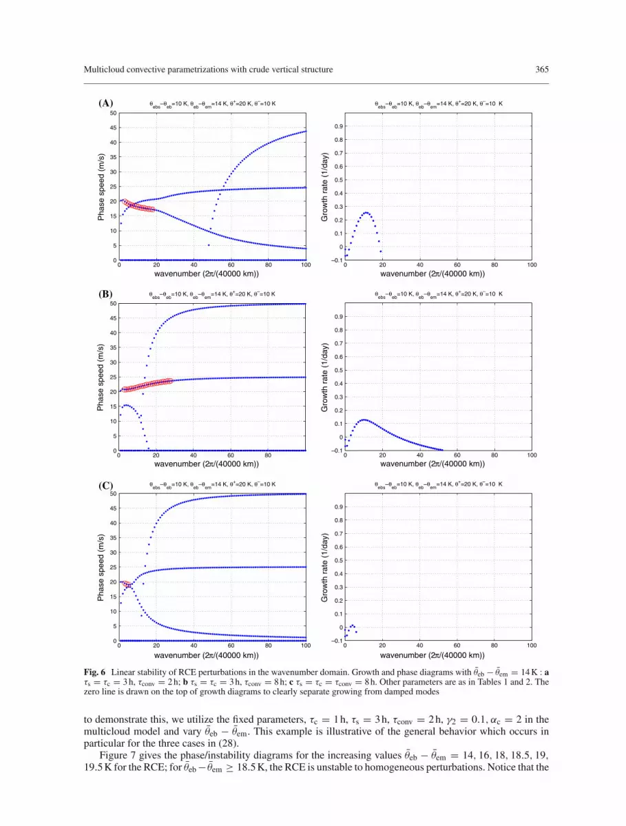
5.1 The effect of time scales in the parametrization on instability

Here we consider the growth rate and phase speed of unstable waves for the standard RCE [37] with θeb−θem =14 K with γ2 = 0.1 and αc = 0.5. According to (18), we consider the following cases

(1) τs = τc = 3 h, τconv = 2 h

(2) τs = τc = 3 h, τconv = 8 h

(3) τs = τc = 8 h, τconv = 8 h(28)

Figure 6 presents the growth rate and phase speed of the unstable waves for these three cases with the standardvalues in Tables 1, and 2. Here and below, the wavenumbers are calculated relative to the natural length scaleL = 40,000 km, which is the circumference of the equator while the unstable waves are marked by circles inthe phase velocity diagrams. Several trends are evident; in all three cases, the instabilities are confined to scaleslarger than 1,500 km and are associated with phase speeds in the range of 15–25 m/s. Furthermore, successivelyincreasing the time-scales from (1) to (2) to (3), results in smaller growth rates for this instability as mightbe anticipated from (17) since the amplitudes of crucial source terms are reduced. The case with τc = 1 h,τs = 3 h, τconv = 2 h has already been discussed extensively in [37] by the authors including its detailed phys-ical structure which strongly resembles the moist convectively coupled gravity waves seen in observations[37–39]; the physical structure of the waves in the three cases in (28) is similar and will not be repeated here.

5.2 Moisture waves for homogeneous unstable RCE’s

For higher values of θeb − θem for which the RCE is unstable to homogeneous perturbations, the stabilityand phase diagrams corresponding to Fig. 6 bifurcate drastically as θeb − θem varies and display remarkablycomplex behavior with the emergence of other families of unstable moisture waves at various scales. Below,


0 20 40 60 80 1000

5

10

15

20

25

30

35

40

45

50

wavenumber (2π/(40000 km))

Pha

se s

peed

(m

/s)

θebs

–θeb

=10 K, θeb

–θem

=14 K, θ+=20 K, θ–=10 K

0 20 40 60 80 100–0.1

0

0.1

0.2

0.3

0.4

0.5

0.6

0.7

0.8

0.9


Gro

wth

rat

e (1

/day

)

θebs

–θeb

=10 K, θeb

–θem

=14 K, θ+=20 K, θ–=10 K

0 20 40 60 800

5

10

15

20

25

30

35

40

45

50


Pha

se s

peed

(m

/s)

θebs

–θeb

=10 K, θeb

–θem

=14 K, θ+=20 K, θ–=10 K

0 20 40 60 80 100–0.1

0

0.1

0.2

0.3

0.4

0.5

0.6

0.7

0.8

0.9


Gro

wth

rat

e (1

/day

)

θebs

–θeb

=10 K, θeb

–θem

=14 K, θ+=20 K, θ–=10 K

0 20 40 60 80 1000

5

10

15

20

25

30

35

40

45

50


Pha

se s

peed

(m

/s)

θebs

–θeb

=10 K, θeb

–θem

=14 K, θ+=20 K, θ–=10 K

0 20 40 60 80 100–0.1

0

0.1

0.2

0.3

0.4

0.5

0.6

0.7

0.8

0.9


Gro

wth

rat

e (1

/day

)

θebs

–θeb

=10 K, θeb

–θem

=14 K, θ+=20 K, θ–=10 K

(A)

(B)

(C)

Fig. 6 Linear stability of RCE perturbations in the wavenumber domain. Growth and phase diagrams with θeb − θem = 14 K : aτs = τc = 3 h, τconv = 2 h; b τs = τc = 3 h, τconv = 8 h; c τs = τc = τconv = 8 h. Other parameters are as in Tables 1 and 2. Thezero line is drawn on the top of growth diagrams to clearly separate growing from damped modes

to demonstrate this, we utilize the fixed parameters, τc = 1 h, τs = 3 h, τconv = 2 h, γ2 = 0.1, αc = 2 in themulticloud model and vary θeb − θem. This example is illustrative of the general behavior which occurs inparticular for the three cases in (28).

Figure 7 gives the phase/instability diagrams for the increasing values θeb − θem = 14, 16, 18, 18.5, 19,19.5 K for the RCE; for θeb − θem ≥ 18.5 K, the RCE is unstable to homogeneous perturbations. Notice that the


0 20 40 60 80 1000

5

10

15

20

25

30

35

40

45

50


Pha

se s

peed

(m

/s)

θebs

–θeb

=10 K, θeb

–θem

=14 K, θ+=20 K, θ–=10 K

0 50 100 150 200–0.1

0

0.1

0.2

0.3

0.4

0.5

0.6

0.7

0.8

0.9


Gro

wth

rat

e (1

/day

)

θebs

–θeb

=10 K, θeb

–θem

=14 K, θ+=20 K, θ–=10 K

0 20 40 60 80 1000

5

10

15

20

25

30

35

40

45

50


Pha

se s

peed

(m

/s)

θebs

–θeb

=10 K, θeb

–θem

=16 K, θ+=20 K, θ–=10 K

0 50 100 150 200–0.1

0

0.1

0.2

0.3

0.4

0.5

0.6

0.7

0.8

0.9


Gro

wth

rat

e (1

/day

)

θebs

–θeb

=10 K, θeb

–θem

=16 K, θ+=20 K, θ–=10 K

0 20 40 60 80 1000

5

10

15

20

25

30

35

40

45

50


Pha

se s

peed

(m

/s)

θebs

–θeb

=10 K, θeb

–θem

=18 K, θ+=20 K, θ–=10 K

0 50 100 150 200–0.2

0

0.2

0.4

0.6

0.8


Gro

wth

rat

e (1

/day

)

θebs

–θeb

=10 K, θeb

–θem

=18 K, θ+=20 K, θ–=10 K

(A)

(B)

(C)

Fig. 7 Same as Fig. 6 except for τs = 3 h, τc = 1 h, τconv = 2 h, and αc = 2 are fixed while θeb − θem varies

unstable phase diagram begins to bifurcate at θeb − θem = 16 K from the standard case at θeb − θem = 14 K; atthis value, a new band of unstable moist gravity waves appears at mesoscopic scales centered around 666 km(wavenumber 60) moving at essentially the dry second baroclinic gravity wave speed of 25 m/s.

The physical structure of the eastward unstable wave at wavelength 666 km is presented in Fig. 8 throughbar diagrams for the unstable eigenvector component amplitudes [34,35,37] as well as traces of quantities ofinterest through one ad one-half spatial periods. Although this wave is moving at the second baroclinic dry


0 20 40 60 80 1000

5

10

15

20

25

30

35

40

45

50


Pha

se s

peed

(m

/s)

θebs

–θeb

=10 K, θeb

–θem

=18.5 K, θ+=20 K, θ–=10 K

0 20 40 60 80 100–0.2

0

0.2

0.4

0.6

0.8


Gro

wth

rat

e (1

/day

)

θebs

–θeb

=10 K, θeb

–θem

=18.5 K, θ+=20 K, θ–=10 K

0 20 40 60 80 1000

5

10

15

20

25

30

35

40

45

50


Pha

se s

peed

(m

/s)

θebs

–θeb

=10 K, θeb

–θem

=19 K, θ+=20 K, θ–=10 K

0 20 40 60 80 100–0.2

0

0.2

0.4

0.6

0.8


Gro

wth

rat

e (1

/day

)

θebs

–θeb

=10 K, θeb

–θem

=19 K, θ+=20 K, θ–=10 K

0 20 40 60 80 1000

5

10

15

20

25

30

35

40

45

50


Pha

se s

peed

(m

/s)

θebs

–θeb

=10 K, θeb

–θem

=19.5 K, θ+=20 K, θ–=10 K

0 20 40 60 80 100

0

0.5

1

1.5

2

2.5

3

3.5

4


Gro

wth

rat

e (1

/day

)

θebs

–θeb

=10 K, θeb

–θem

=19.5 K, θ+=20 K, θ–=10 K

(D)

(E)

(F)

Fig. 7 Contd.

gravity wave speed and has a significant second baroclinic structure it is strongly convectively coupled withprominent moisture, congestus, stratiform, and first baroclinic mode components. It has a structure resemblingthose discussed by Mapes [9] which act as triggers for additional organized mesoscale convection. Further-more, congestus peaks lead moisture peaks which lead deep convective peaks as illustrated in Figs. 8 d, e.At the value, θeb − θem = 18.5 K, a new band of slower large scale moist gravity waves emerges. Notice the


movement of the band on instability of the 25 m/s waves. For the even larger value with θeb − θem = 19 K thereis moist gravity waves with maximum phase speed of 15 m/s on planetary to synoptic scales (2 ≤ k ≤ 20)asymptotically converging to moist gravity waves with nearly zero phase velocity and constant growth rate atsmall scales (k ≥ 30) while the 25 m/s instability weakens a great deal moves back toward the small scalesand ultimatly desapears.

The structure of the slow moving westward propagating moist gravity wave with wavelength 666 km andphase velocity 1.26 m/s is shown in Fig. 9; the wave is dominated by moisture and θeb fluctuations (largeCAPE) and has a deep convective structure with both first and second baroclinic components with moisture

0

0.2

0.4

0.6

0.8

1Growth=0.0013913 1/day, speed=24.4597 m/s

V1

V2

θ1

θ2

θeb q H

sH

c

0 250 500 750 10000

4

8

12

16

X (km, One wavelength = 666 km)

Dep

th

LargeScale Flow, U, W, and potential temperature contours

0 250 500 750 10000

4

8

12

16

Dep

th

Regions of Convective Heating and Cooling Anomalies

0 250 500 750 1000–1

0

1 θeb

qθ

eb–θ

em

0 250 500 750 1000–1

0

1

X (km, One wavelength =666 km)

PDHsHc

(A)

(B)

(C)

(D)

(E)

Fig. 8 Physical structure of eastward 25 m/s−1 moist gravity wave at wavenumber k = 60. θeb − θem = 16 K, τs = 3 h, τc = 1 h,τconv = 2 h, αc = 2. Other parameters are as in Tables 1 and 2. a bar diagram of eigenmode component amplitudes. x-z Contoursof potential temperature b and convective heating field c with velocity arrows overlaid


peaks leading deep convective peaks. (Notice from the bar diagram that u1 is slightly larger than u2 leadingto a strong shear and strong winds near the surface and aloft.) Also because of its slow propagation speed,the slope in the (total) upward motion of nearly one (resulting from the 3 h stratiform lag: 1.26 m/s × 3 h =13 km) is much smaller than the slope observed for the 15 m/s convectively coupled Kelvin wave analogues[34,35,37]. Given the aspect ratio on Fig. 9, this yields a nearly vertical upward motion at the center of thedeep convection and an upraising of the air near the surface. These features of the slow moving wave in Fig. 9,just summarized above, including the spatial structure (strong shear, slope one of upward motion, upraising ofnear surface air, strong surface winds immediately in front and in the back of the convective region, etc.), thephase speed, and the length scale are reminiscent of a westward propagating squall line [46].

0

0.2

0.4

0.6

0.8

1Growth=0.61569 1/day, speed=1.2583 m/s

V1 V2θ1 θ2 θeb q Hs Hc

0 250 500 750 10000

4

8

12

16


Dep

th


0 250 500 750 10000

4

8

12

16

Dep

th


0 250 500 750 1000–1

0

1 θeb

qθ

eb–θ

em

0 250 500 750 1000–1

0

1


PDHsHc

(A)

(B)

(C)

(D)

(E)

Fig. 9 Same as Fig. 8 except for the slow westward propagating moist gravity at wavenumber k = 60, θeb − θem = 19 K, τs = 3 h,τc = 1 h, τconv = 2 h, αc = 2


Finally, at the largest value of θeb−θem = 19.5 K, the unstable phase diagram undergoes another bifurcationto two standing waves of instability over the entire range of wavenumber k ≥ 2 while at wavenumber one wehave the instability of two convectively coupled waves moving at roughly 13 m/s. The structure of the standingmode with the larger growth rates is shown in Fig. 10. The second standing mode has a similar structure.From Fig. 10 we see that these standing modes are essentially deep convective standing waves with the firstbaroclinic components dominating. Notice the air rising near the surface directly to the top of the troposphereat the locations of maximum heating and warm temperatures in Figs. 10b, c. The streamlines are on the formof Rayleigh-Benard convective cells. From Figures 10d, e, all the thermodynamic variables and forcing terms(q, θeb, θem, P, H,Hc, and D) are perfectly correlated with each other confirming the non-propagating natureof the wave.

0

0.2

0.4

0.6

0.8

1Growth=2.214 1/day, speed=5.2735e14 m/s

V1

V2

θ1

θ2

θeb q H

sH

c

0 3000 6000 9000 120000

4

8

12

16


Dep

th


0 3000 6000 9000 120000

4

8

12

16

Dep

th


0 3000 6000 9000 12000–1

0

1θ

ebqθ

eb–θ

em

0 3000 6000 9000 12000–1

0

1


PDHsHc

(A)

(B)

(C)

(D)

(E)

Fig. 10 Same as Fig. 9 except for θeb − θem = 19.5 K, for the standing mode with larger growth rate at wavenumber k = 5


6 Concluding discussion

Here we have discussed a variety of new aspects of the multicloud parametrizations with two vertical baroclinicmodes introduced recently by the authors [37–39]. In Sect. 3, we clarified all of the relevant time scales in thesemodels and showed how variants of other more familiar parametrization schemes involving a single verticalbaroclinic mode arise as limiting special cases. One of the new phenomena in the multi-cloud parametrizationsis the existence of suitable unstable RCE’s involving a large fraction of congestus clouds and smaller fraction ofdeep convective clouds. Various novel aspects of the linear and nonlinear instability of such RCE’s are studiedhere in Sects. 4, and 5. In Sect. 4, the nonlinear instability of unstable RCE’s to homogeneous perturbations isstudied with three different types of dynamics involving nonlinear adjustment to a deep convective dominated–stable RCE (Fig. 3), periodic oscillations (Fig. 4), and even heteroclinic chaos (Fig. 5). In Sect. 5, the linearinstability of unstable RCE’s to perturbations with general spatial structure is analyzed. Besides the large scaleconvectively coupled gravity waves [37], new modes of instability arise including mesoscale second baroclinicmoist gravity waves [9], slow moving mesoscale “squall line modes”, and large scale standing modes. Therole of the basic convective adjustment time scales, τc, τs, τconv, on linearized stability is also clarified.

Acknowledgements The research of B.K. is supported by a University of Victoria Start-up grant and a grant from the NaturalSciences and Engineering Research Council of Canada. The research of A.M. is partially supported by ONR N0014-96-1-0043,NSF DMS-0456713, and NSF-FRG DMS-0139918. The authors are thankful to M.W. Moncrieff for sponsoring a visit for B.K.to NCAR during the summer of year 2004 where this work was partly initiated.

Appendix: Derivation of the vertically integrated moisture equation

Recall the bulk water budget equations in the atmosphere [16]

∂qv

∂t+ div(Vqv)+ ∂(wqv)

∂z= Ev − C

∂qc

∂t+ div(Vqc)+ ∂(wqc)

∂z= C − Ev − Ar (29)

∂qr

∂t+ div(Vqr)+ ∂(wqr)

∂z− ∂(vtqr)

∂z= Ar

where qv, qc, qr are the mixing ratios of water vapor, cloud water, and rain, respectively, Ev,C, Ar are therates of evaporation, condensation, conversion of cloud water into rain, respectively, and vt is the fall speedof precipitation (notice the minus sign in front). The quantities V and w represent, respectively, the horizon-tal and vertical (incompressible) velocity components while div denotes the horizontal divergence operator:div(u1, u2) = ∂x u1 + ∂yu2.

At the large time (and spatial) scales of interest of a few days (and a few hundreds of kilometers) thedynamics of both cloud water and rain are simplified (averaged out) by assuming that clouds and rain occur atsmaller scales. Therefore we assume a quasi-equilibrium where

Ar = −∂(vtqr)

∂zand C = Ev + Ar

where the overbar represents the long-time average.Introducing these new settings into the first equation in (30) we obtain the large scale equation for qv:

∂qv

∂t+ div(Vqv)+ ∂(wqv)

∂z= ∂(vtqr)

∂z(30)

where the turbulent fluxes are ignored. Assume that the (total) water vapor, qv, decomposes onto

qv(x, y, z, t) = Q(z)+ q(x, y, z, t);a horizontal/time homogeneous vertical profile background (moisture stratification), Q(z), plus a perturba-tion, q .


We introduce the vertical average of the water vapor perturbation

〈q〉 := 1

HT

HT∫

0

q dz (31)

where HT is the height of the troposphere. Let P be the rate of precipitation which reaches the ground as thevertical average of the long time averaged precipitation flux :

P = − 1

HT

HT∫

0

∂(vtqr)

∂zdz = 1

HTvtqr

∣∣∣∣z=0

,

assuming that on average qr and vt are zero at the top of the troposphere z = HT.By applying the average in (31) to the equation in (30) we obtain

∂ 〈q〉∂t

+ 〈div(Vq)〉 +⟨w

dQ(z)

dz

⟩+ 1

HT(wq)

∣∣∣∣z=HT

z=0= −P. (32)

By assuming that q(HT) ≈ 0; the water vapor content is negligible at the top of the troposphere, we get

1

HT(wqv)

∣∣∣∣z=HT

z=0≈ − 1

HT(wqv)

∣∣∣∣z=0

= − 1

HTFq

−

where Fq− represents the net supply of water vapor from the surface. Thus the equation in (32) is rewritten as

∂ 〈q〉∂t

+ 〈div(Vq)〉 +⟨w

dQ(z)

dz

⟩= Fq

− − P. (33)

Case of two baroclinic mode models

When the governing (primitive) equations are Galerkin projected onto the first two baroclinic vertical modesplus a barotropic mode, the velocity field takes the form

V = v + v1√

2 cos

(π z

HT

)+ v2

√2 cos

(2π z

HT

)

and

w = −√

2HT

π

(div v1 sin

(π z

HT

)+ 1

2div v2 sin

(2π z

HT

))

where v1, v2 are, respectively, the first and second baroclinic velocity components and v is the barotropic part.Plugging the formulas for V and w into the equation in (33) yields

∂ 〈q〉∂t

+ v · ∇ 〈q〉 + div(v1φ(q))+ div(v2ψ(q))+ Q(divv1 + λdivv2) = Fq− − P (34)

where

φ(q) =√

2

HT

HT∫

0

q cos

(π z

HT

)dz; ψ(q) =

√2

HT

HT∫

0

q cos

(2π z

HT

)dz (35)

and

Q = −√

2

π

HT∫

0

dQ(z)

dzsin

(π z

HT

)dz; λ = −

√2

2Qπ

HT∫

0

dQ(z)

dzsin

(2π z

HT

)dz. (36)


Closures for φ(q), ψ(q), Q, and λ in (36)

By assuming plausible vertical profiles for Q(z) and q we derive here some rough estimates for the quantitiesφ(q), ψ(q), Q, and λ in (36). We start with Q and λ. The observed vertical distribution of water vapor inthe tropics (for e.g. see [46] or [51]) suggests a profile for Q(z) which is rapidly decreasing in the lowertroposphere and asymptotically vanishing aloft. For simplicity we assume an exponential form profile,

Q(z) = q0 exp(−z/Hq), (37)

where Hq is the e-folding distance or the moisture scale hight and q0 a constant representing the value of q atthe surface z = 0. We have, from (36),

Q =√

2q0

πHq

HT∫

0

e−z/Hq sin

(π z

HT

)dz =

√2q0

HT/Hq + π2 Hq/HT

(1 + e−HT/Hq

)

and

λQ =√

2q0

2πHq

HT∫

0

e−z/Hq sin

(2π z

HT

)dz =

√2q0

HT/Hq + 4π2 Hq/HT

(1 − e−HT/Hq

), (38)

which yield

λ(Hq/HT) = 1 + π2(Hq/HT)2

1 + 4π2(Hq/HT)2tanh

(1

2Hq/HT

);

a monotonically decreasing function of Hq/HT with the upper-bound

λ ≤ limHq/HT−→0

λ(Hq/HT) = 1,

if for the example Hq/HT = 1/8, then we get λ = 0.7135. Therefore, values of λ ranging from λ = 0.7 toλ = 1 are plausible, in our case we pick the conservative value of λ = 0.8. Moreover, note that Q dependslinearly on the surface moisture q0 therefore it can take any arbitrary value. For our calculations we use thestandard value of Q = 0.9 also used in [16,42,43,52].

Now we return to φ(q) and ψ(q). We seek closures on the form

φ(q) = α1 〈q〉 ; and ψ(q) = α2 〈q〉 (39)

where α1 and α2 are constants. We assume separation of variables

q(x, y, z, t) = q1(z)q2(x, y, t). (40)

Therefore

〈q〉 = 〈q1〉 q2, (41)

then provided that 〈q1〉 = 0, we have

α1 =√

2

HT 〈q1〉HT∫

0

q1(z) cos

(π z

HT

)dz,

and

α2 =√

2

HT 〈q1〉HT∫

0

q1(z) cos

(2π z

HT

)dz.


If we assume that the bulk of the moisture variability is concentrated within the lower half 0 ≤ z ≤ HT/2of the troposphere then we can apply the mean value theorem for the first integral and get

α1 ≈√

2

HT 〈q1〉

HT/2∫

0

q1(z) cos

(π z

HT

)dz = q1(zl)

√2

HT 〈q1〉

HT/2∫

0

cos

(π z

HT

)dz ≈ 2

√2

π= 0.9003 ≈ 1.

where 0 ≤ zl ≤ HT/2 and we assumed 〈q1〉 ≈ q1(zl) to a first approximation. For α2, we use a simplemidpoint quadrature rule on the lower half of the troposphere leading to

α2 ≈√

2

HT 〈q1〉

HT/2∫

0

q1(z) cos

(2π z

HT

)dz ≈

√2

2

q1(HT/4)

〈q1〉 cos(π

2

)= 0.

The extreme situation where the above approximation would fail occurs when q1(z) is correlated with cos( 2π zHT),

i.e, q1(z) ≈ q0 cos( 2π zHT). This yields

〈q1〉 ≈ 0

in which case our assumption 〈q1〉 = 0 is not valid thus leading to undetermined values for α1, α2. Neverthe-less, we believe that such a situation is very unlikely in nature and therefore, overall, we will have an effectiveα2 << 1. Therefore, in our nonlinear simulations using the system in (1), we use the values

α1 = 1, α2 = 0.1.

With the values of λ, α1, α2 given, (34) yields the moisture equation used in the multicloud parametrizationswith the angle brackets omitted for simplicity in exposition.

References

1. Nakazawa, T.: Tropical super clusters within intraseasonal variations over the western pacific. J. Meteorol. Soc. Jpn. 66,823–839 (1988)

2. Hendon, H.H., Liebmann, B.: Organization of convection within the Madden–Julian oscillation. J. Geophys. Res. 99, 8073–8083 (1994)

3. Wheeler, M., Kiladis, G.N.: Convectively coupled equatorial waves: Analysis of clouds and temperature in the wavenum-ber-frequency domain. J. Atmos. Sci. 57, 613–640 (1999)

4. Emanuel, K.A., Raymond, D.J.: The representation of Cumulus convection in numerical models. In: Meteorological mono-graphs, vol. 84, Boston: American Meterological Society, 1993

5. Smith, R.K: The physics and parametrization of moist atmospheric convection. NATO ASI, Kluwer, Dordrecht, 19976. Slingo, J.M. et al.: Intraseasonal oscillation in 15 atmospheric general circulation models: results from an amip diagnostic

subproject. Climate Dyn. 12, 325–357 (1996)7. Moncrieff, M.W., Klinker, E.: Organized convective systems in the tropical western pacific as a process in general circulation

models: a toga-coare case study. Q. J. Roy. Meteorol. Soc. 123, 805–827 (1997)8. Emanuel, K.A.: An air-sea interaction model of intraseasonal oscillations in the tropics. J. Atmos. Sci. 44, 2324–2340 (1987)9. Mapes, B.E.: Gregarious tropical convection. J. Atmos. Sci. 50, 2026–2037 (1993)

10. Neelin, D., Yu, J.: Modes of tropical variability under convective adjustment and the Madden–Julian oscillation. Part I:analytical theory. J. Atmos. Sci. 51, 1876–1894 (1994)

11. Yano, J.-I., McWilliams, J., Moncrieff, M., Emanuel, K.A.: Hierarchical tropical cloud systems in an analog shallow-watermodel. J. Atmos. Sci. 48, 1723–1742 (1995)

12. Yano, J.-I., Moncrieff, M., McWilliams, J.: Linear stability and single-column analyses of several cumulus parametrizationcategories in a shallow-water model. Q. J. Roy. Meteorol. Soc. 124, 983–1005 (1998)

13. Majda, A., Shefter, M.: Waves and instabilities for model tropical convective parametrizations. J. Atmos. Sci. 58, 896–914(2001)

14. Majda, A.J., Khouider, B.: Stochastic and mesoscopic models for tropical convection. Proc. Natl. Acad. Sci. USA 99,1123–1128 (2002)

15. Fuchs, Z., Raymond, D.: Large-scale modes of a nonrotating atmosphere with water vapor and cloud-radiation feedbacks. J.Atmos. Sci. 59, 1669–1679 (2002)

16. Frierson, D., Majda, A., Pauluis, O.: Dynamics of precipitation fronts in the tropical atmosphere: a novel relaxation limit.Commun. Math. Sci. 2, 591–626 (2004)

17. Charney, J.G., Eliassen, A.: On the growth of the hurricane depression. J. Atmos. Sci. 21, 68–75 (1964)18. Yamasaki, M.: Large-scale disturbances in a conditionally unstable atmosphere in low latitudes. Pap. Meteor. Geophys. 20,

289–336 (1969)


19. Hayashi, Y.: Large-scale equatorial waves destabilized by convective heating in the presence of surface friction. J. Meteor.Soc. Jpn. 49, 458–466 (1971)

20. Lindzen, R.S.: Wave-cisk in the tropics. J. Atmos. Sci. 31, 156–179 (1974)21. Arakawa, A., Shubert, W.H.: Interaction of a cumulus cloud ensemble with the large-scale environment. Part i. J. Atmos.

Sci. 31, 674–701 (1974)22. Emanuel, K.A., Neelin, J.D., Bretherton, C.S.: On large-scale circulations in convecting atmosphere. Q. J. Roy. Meteor. Soc.

120, 1111–1143 (1994)23. Lin, X., Johnson, R.H.: Kinematic and thermodynamic characteristics of the flow over the western pacific warm pool during

toga coare. J. Atmos. Sci. 53, 695–715 (1996)24. Johnson, R.H., Rickenbach, T.M., Rutledge, S.A., Ciesielski, P.E., Schubert, W.H.: Trimodal characteristics of tropical

convection. J. Climate 12, 2397–2407 (1999)25. Straub, K.H., Kiladis, G.N., Observations of a convectively-coupled kelvin wave in the eastern pacific itcz. J. Atmos. Sci.

59, 30–53 (2002)26. Haertl, P.T., Kiladis, G.N.: On the dynamics of two day equatorial disturbances. J. Atmos. Sci. 61, 2707–2721 (2004)27. Kiladis, G.N., Straub, K.H., Haertl, P.: Zonal and vertical structure of the Madden–Julian oscillation. J. Atmos. Sci. 62,

2790–2809 (2005)28. Dunkerton, T.J., Crum, F.X.: Eastward propagating 2- to 15-day equatorial convection and its relation to the tropical

intraseasonal oscillation. J. Geophys. Res. 100, 25781–25790 (1995)29. Majda, A., Biello, J.: A multi-scale model for the intraseasonal oscillation. Proc. Natl. Acad. Sci. 101, 4736–4741 (2004)30. Biello, J., Majda, A.: A multi-scale model for the madden–julian oscillation. J. Atmos. Sci. 62, 1694–1721 (2005)31. Zehnder, J.: A comparison of convergence- and surface-flux-based convective parametrizations with applications to tropical

cyclogenesis. J. Atmos. Sci. 58, 283–301 (2001)32. Craig, G.C., Gray, S.L.: CISK or WISHE as the mechanism for tropical cyclone intensification. J. Atmos. Sci. 53, 3528–3540

(1996)33. Mapes, B.E.: Convective inhibition, subgridscale triggering energy, and “stratiform instability” in a toy tropical wave model.

J. Atmos. Sci. 57, 1515–1535 (2000)34. Majda, A., Shefter, M.: Models for stratiform instability and convectively coupled waves. J. Atmos. Sci. 58, 1567–1584

(2001)35. Majda, A., Khouider, B., Kiladis, G.N., Straub, K.H., Shefter, M.: A model for convectively coupled tropical waves: nonlin-

earity, rotation, and comparison with observations. J. Atmos. Sci. 61, 2188–2205 (2004)36. Yano, J.-I., Emanuel, K.: An improved model of the equatorial troposphere and its coupling to the stratosphere. J. Atmos.

Sci. 18, 377–389 (1991)37. Khouider, B., Majda, A.J.: A simple multicloud parametrization for convectively coupled tropical waves. Part i: linear

analysis. J. Atmos. Sci. 63 pp. 1308–1323 (2006)38. Khouider, B., Majda, A.J.: A simple multicloud parametrization for convectively coupled tropical waves. Part ii: nonlinear

simulations. J. Atmos. Sci. (2006, in press)39. Khouider, B., Majda, A.J.: Model multicloud parametrizations for convectively coupled waves: detailed nonlinear wave

evolution. Dynam. Atmos. Oceans (2006, in press)40. Neelin, D., Zeng, N.: A quasi-equilibrium tropical circulation model–formulation. J. Atmos. Sci. 57, 1741–1766 (2000)41. Majda, A., Biello, J.: The nonlinear interaction of barotropic and equatorial baroclinic Rossby waves. J. Atmos. Sci. 60,

1809–1821 (2003)42. Khouider, B., Majda, A.J.: A non-oscillatory well balanced scheme for an idealized tropical climate model. Part I: Algorithm

and validation. Theor. Comput. Fluid Dyn. 19, 331–354 (2005)43. Khouider, B., Majda, A.J.: A non-oscillatory well balanced scheme for an idealized tropical climate model. Part II: Nonlinear

coupling and moisture effects. Theor. Comput. Fluid Dyn. 19, 355–375 (2005)44. Gill, A.: Atmosphere-ocean dynamics. International geophysics series, vol. 30. Academic, New York, (1982)45. Betts, A.K., Miller, M.J.: A new convective adjustemnt scheme. Part ii: single column tests using gate wave, bomex, and

arctic air-mass data sets. Q. J. Roy. Meteorol. Soc. 112, 693–709 (1986)46. Emanuel, K.: Atmospheric convection. Oxford University Press, Oxford, (1994)47. Betts, A.K.: A new convective adjustemnt scheme. part i: Observational and theoretical basis. Q. J. Roy. Meteorol. Soc. 112,

677–692 (1986)48. Bretherton, C.S., Peters, M.E., Back, L.E.: Relationship between water vapor path and precipitation over the tropical oceans.

J. Climate 17, 1517–1528 (2004)49. Armbuster, D.J., Guckenheimer, J., Holmes, P.: Heteroclinic cycles and modulated traveling waves in systems with O(2)

symmetry. Phys. D 29, 257–282 (1988)50. Holmes, P., Lumley, J.L., Berkooz, G.: Turbulence, coherent structures, dynamical systems, and symmetry. Cambridge

University Press, New York, (1996)51. Pruppacher, H.R, Klett, J.D.: Microphysics of clouds and precipitation, chap 12. Kluwer, Dordrecht, (2000)52. Lin, J., Neelin, J.D., Zeng, N.: Maintenance of tropical intraseasonal variability: Impact of evaporation-wind feedback and

midlatitude storms. J. Atmos. Sci. 57, 2793–2823 (2000)

Documents

Multicloud Convective Parametrizations with Crude Vertical Structure