Adsorption (2007) 13: 357–372DOI 10.1007/s10450-007-9028-2

Multiphysics modeling of electric-swing adsorption systemwith in-vessel condensation

Menka Petkovska · Danijela Antov-Bozalo ·Ana Markovic · Patrick Sullivan

Received: 30 April 2007 / Revised: 20 July 2007 / Accepted: 23 July 2007 / Published online: 22 September 2007© Springer Science+Business Media, LLC 2007

Abstract Mathematical modeling of an Electric-Swing Ad-sorption (ESA) system (adsorption cycle with electrother-mal desorption step, performed by direct heating of the ad-sorbent particles by passing electric current through them),with annular, radial-flow, cartridge-type fixed-bed and in-vessel condensation, is performed by using Comsol Multi-physics™ software. Three multiphysics models are built, inorder to describe three stages of a compete ESA cycle: ad-sorption, electrothermal desorption before the start of con-densation and electrothermal desorption with in-vessel con-densation. In order to describe the complete ESA cycle themodels for the three stages are integrated, by using a combi-nation of Comsol Multiphysics™ and Matlab™. The mod-els were successfully used for simulation of separate stagesof the process and of the complete ESA cycles, as well asfor investigation of the influences of the main operationalparameters on the process performance.

The views and conclusions contained herein are those of the authorand should not be interpreted as necessarily representing the officialpolicies or endorsements, either expressed or implied, of the Air ForceOffice of Scientific Research or the U.S. Government.

M. Petkovska (�) · D. Antov-Bozalo · A. MarkovicDepartment of Chemical Engineering, Faculty of Technology andMetallurgy, University of Belgrade, Belgrade, Serbiae-mail: menka@tmf.bg.ac.yu

Present address:A. MarkovicMax-Planck Institute for Dynamics of Complex TechnicalSystems, Sandtorstr. 1, 39106 Magdeburg, Germany

P. SullivanAir Force Research Laboratory, Tyndall AFB, FL, USA

Keywords Multiphysics modeling · Electric-SwingAdsorption (ESA) · Electrothermal desorption · In-vesselcondensation

Abbreviations

a (m2/m3) Specific surface areab (K−1) Temperature coefficient of the bed

electrical resistivityC (mol/mol) Adsorbate concentration in the

gas phaseC∗(mol/mol) Adsorbate concentration in the

gas phase in equilibrium with thesolid phase

Cbreak (mol/mol) Breakthrough concentrationCsat (mol/mol) Saturation concentrationcpg (J/mol/K) Specific heat capacity of the inert

gascpl (J/mol/K) Specific heat capacity of liquid

adsorbatecps (J/g/K) Heat capacity of the solid phasecpv (J/mol/K) Specific heat capacity of gaseous

adsorbateDm (mol/cm/s) Mass transfer dispersion

coefficientD

hgt (W/K/cm) Heat diffusivity of the gas phase

Dhst (W/K/cm) Heat diffusivity of the solid phase

E (J/mol) Adsorption energy of theadsorbate (D-R equation)

g (cm/s2) Gravitation constantG (mol/s) Flow rate of the inert gasH (cm) Bed axial dimension (Fig. 2)h1 (cm) Adsorber dimension (Fig. 2)hb (J/cm2/K) Solid to gas heat transfer

coefficient within the bed

358 Adsorption (2007) 13: 357–372

hs1 (J/cm2/K) Heat transfer coefficient from thesolid phase to the gas phase in thecentral tube(s)

hs2 (J/cm2/K) Heat transfer coefficient from thesolid phase to the gas phase in theannular tube

hwg (J/cm2/K) Gas to ambient heat transfercoefficient (heat losses)

J (A/cm2) Current densityJcond (mol/cm2/s) Condensation fluxk (cm2) Asorbent bed permeabilitykm (mol/cm2/s) Mass transfer coefficient in the

adsorbent bedkm1 (mol/cm2/s) Mass transfer coefficient between

the adsorbent bed and the gas inthe central tube

km2 (mol/cm2/s) Mass transfer coefficient betweenthe adsorbent bed and the gas inthe annular tube

Lcond (mol/s) Flow-rate of the condensed liquidLcond (mol) Total amount of the condensed

liquidp (Pa) Gas pressurepa (Pa) Ambient pressurepc (Pa) Critical pressurep0 (Pa) Adsorbate saturation pressureQel (W) Rate of heat generation (equal to

electric power)Qel (J) Heat generation (equal to electric

energy)q (mol/g) Adsorbate concentration in the

solid phaseRg (J/mol/K) Gas constantr (cm) Radial coordinater1 (cm) Adsorber dimension—radius of

the central tube (Fig. 2)r2 (cm) Adsorber dimension (Fig. 2)r3 (cm) Adsorber dimension (Fig. 2)r4 (cm) Adsorber dimension—radius of

the adsorber vessel (Fig. 2)Sw (cm2) Surface are of the outer wall of

the adsorber vesselT a (K) Ambient temperatureT g (K) Gas phase temperatureTc (K) Critical temperatureT R (K) Referent temperatureT s (K) Solid phase temperatureTsw (K) Switch temperature (from

desorption to adsorption)Tw (K) Wall temperaturet (s) TimeU (V) Electric potentialU0 (V) Supply voltage

u (cm/s) Radial superficial gas velocityV PA, V PB , V PC , V PD Wagner constants (Wagner

equation)v (cm/s) Axial superficial gas velocityW0 (cm3/g) Total volume of micropores (D-R

equation)z (cm) Axial coordinate

Greek letters:

αp Purification factorαs Separation factor�Hads (J/mol) Heat of adsorption�Hcond (J/mol) Heat of condensationεb Bed porosityμ (Pa/s) Dynamic viscosityρ (�cm) Electric resistivityρ0 (�cm) Electric resistivity at referent

temperature TR

ρg (mol/cm3) Gas phase densityρb (g/cm3) Adsorbent bed densityρA (g/cm3) Adsorbate densityτ (s) Time period

Subscripts:

A Adsorptionb BedD Desorptiong Gasin Inletout Outletp Previous (initial)r In the radial (r) directions Solid phasect Central tubeas Annular spacez In the axial (z) direction

Special characters:

〈 〉 Time average value

1 Introduction

Electric (or electrothermal) swing adsorption (ESA) is a rel-atively new name (Yu et al. 2007; Sullivan et al. 2004a) foran essentially temperature-swing adsorption (TSA) cycle inwhich the adsorbent material is heated by passing electriccurrent through it (owing to Joule effect).

The idea about regeneration of used adsorbent beds bydirect heating by electric current was first published in the1970s (Fabuss and Dubois 1970). The desorption processbased on this principle was later named electrothermal des-orption (Petkovska et al. 1991) and it was recognized as a

Adsorption (2007) 13: 357–372 359

prospective way to perform desorption steps of TSA cycles(Petkovska et al. 1991).

The main differences between electrothermal desorptionand classical techniques of thermal regeneration of used ad-sorpbents (e.g. heating by hot gas or steam) are (Sullivan2003; Petkovska and Mitrovic 1994a, 1994b):

• Energy efficiency is higher than when heating by steamor inert gas, because the energy is delivered directly tothe adsorbent, thus minimizing the energy expended forheating of the vessel and ancillary equipment.

• Heating rate of the adsorbent is not limited by heat/masstransfer rates between the carrier gas and the adsor-bent, because the energy is directly applied to the ad-sorbent rather than being delivered by the carrier gasstream.

• Effluent concentration of adsorbate can be maximized,because the purge gas flow rate is controlled indepen-dently from the power applied to the adsorbent.

• Unlike steam regeneration, no water is introduced intothe system, which is difficult and costly to separate fromwater-miscible adsorbates, and which can cause corro-sion.

• The directions of heat and mass transfer are identical inthe case of electrothermal desorption, and opposite in thecase of conventional thermal desorption by hot gas orsteam. This can influence the process kinetics and dy-namics.

It was shown that electrothermal desorption has some advan-tages over conventional methods, regarding adsorption ki-netics and dynamics (Petkovska and Mitrovic 1994a, 1994b)and energy efficiency (Petkovska et al. 1991; Sullivan 2003).

Most applications of electrothermal desorption have beenbased on fibrous activated carbon materials (Petkovska et al.1991; Rood et al. 2002; Sullivan et al. 2001, 2004a, 2004b;Subrenat and Le Cloirec 2004, 2006; Moon and Shim 2006;Luo et al. 2006), although granular activated carbons (Sny-der and Leesch 2001; Sushchev et al. 2002; Luo et al. 2006)and, recently, carbon monoliths (Luo et al. 2006; Yu et al.2002, 2007), have also been used.

Up to now, different applications (mostly on laboratoryscale) of regeneration of used adsorbents by electrother-mal desorption have been reported: air purification, withemphases on removal of hazardous volatile organic com-pounds (Baudu et al. 1992; Azou et al. 1993; Sullivan etal. 2001, 2003; Subrenat and Le Cloirec 2006), gas separa-tion (Moon and Shim 2006) and solvent recovery (Bathenet al. 1997; Lordgooei et al. 1996; Snyder and Leesch 2001;Sullivan 2003). In the last couple of years, some applica-tions of electrothermal desorption on industrial scale havealso been reported (Bathen 2002; Subrenat and Le Cloirec2004, 2006).

The subject of this investigation is mathematical mod-eling of an ESA system based on assembly of annular,

radial-flow, cartridge-type fixed-beds, with in-vessel con-densation (Rood et al. 2002; Sullivan 2003; Sullivan et al.2004a), which has been developed for removal and recov-ery of hazardous volatile organic compounds. This systeminvolves a large number of coupled processes and phenom-ena: fluid flows through tubes and porous beds, adsorption,mass transfer, heat transfer, heat generation associated withelectric current flow, and condensation, all in a rather com-plex geometry. Such a system is very demanding from themodeling point of view and represents a good candidate formultiphysic modeling. This manuscript presents the proce-dure and results of mathematical modeling of this system byusing Comsol Multiphysics™, a software tool specializedfor multiphysics modeling.

2 Description of the modeled system

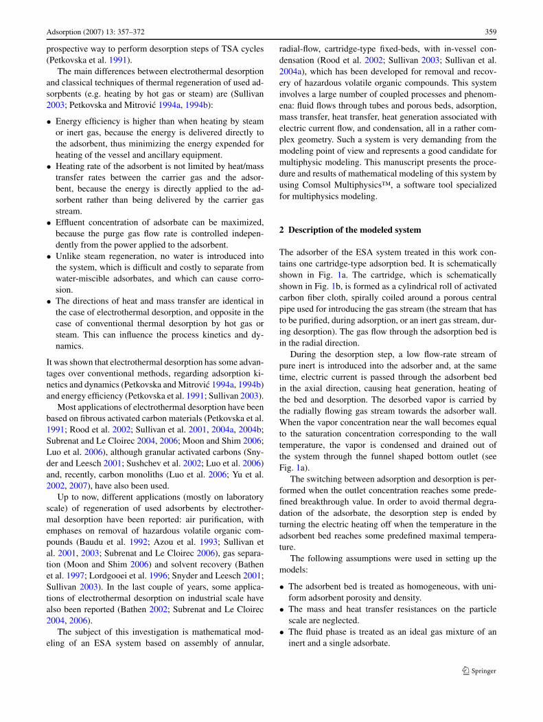
The adsorber of the ESA system treated in this work con-tains one cartridge-type adsorption bed. It is schematicallyshown in Fig. 1a. The cartridge, which is schematicallyshown in Fig. 1b, is formed as a cylindrical roll of activatedcarbon fiber cloth, spirally coiled around a porous centralpipe used for introducing the gas stream (the stream that hasto be purified, during adsorption, or an inert gas stream, dur-ing desorption). The gas flow through the adsorption bed isin the radial direction.

During the desorption step, a low flow-rate stream ofpure inert is introduced into the adsorber and, at the sametime, electric current is passed through the adsorbent bedin the axial direction, causing heat generation, heating ofthe bed and desorption. The desorbed vapor is carried bythe radially flowing gas stream towards the adsorber wall.When the vapor concentration near the wall becomes equalto the saturation concentration corresponding to the walltemperature, the vapor is condensed and drained out ofthe system through the funnel shaped bottom outlet (seeFig. 1a).

The switching between adsorption and desorption is per-formed when the outlet concentration reaches some prede-fined breakthrough value. In order to avoid thermal degra-dation of the adsorbate, the desorption step is ended byturning the electric heating off when the temperature in theadsorbent bed reaches some predefined maximal tempera-ture.

The following assumptions were used in setting up themodels:

• The adsorbent bed is treated as homogeneous, with uni-form adsorbent porosity and density.

• The mass and heat transfer resistances on the particlescale are neglected.

• The fluid phase is treated as an ideal gas mixture of aninert and a single adsorbate.

360 Adsorption (2007) 13: 357–372

(a)

(b)

Fig. 1 Schematic representation of: (a) the adsorber with car-tridge-type adsorbent bed and in-vessel condensation; and (b) the an-nular, radial-flow cartridge

• The electric resistivity of the adsorbent is temperature

dependent. Linear temperature dependence is assumed,

based on experimental results reported in (Sullivan 2003).

• All other physical parameters and coefficients are consid-

ered as constants.

• The condensation at the adsorber wall is dropwise. This

assumption is based on experimental observations re-

ported in Sullivan (2003).

• The volume of the condensed liquid is neglected, i.e., it is

assumed that the liquid drops don’t influence the gas flow.

• The heat resistance and heat capacity of the adsorber wall

are neglected, so the wall temperature is regarded as equal

to the temperature of the environment.

• Heat transfer by radiation is neglected.

• The electric power during electrothermal desorption is

supplied under constant voltage conditions.

3 Multiphysics models for separate steps of the ESAcycle

Analysis of the adsorber defined in the previous sectionshows that it consists of three parts: the central tube used forintroducing the gas, the adsorbent bed and the annular spacebetween the adsorbent bed and the outer adsorber wall. Also,three consecutive steps of the complete ESA cycle with in-vessel condensation can be defined:

• Adsorption;• Desorption without condensation;• Desorption accompanied with condensation.

The last two steps are parts of the desorption half-cycle.The mathematical model of the system consists of the

momentum, mass and heat balances for different parts of thesystem (the central tube of the cartridge, the adsorbent bedand the annular space around the cartridge) and for the gasand solid phases, as well as the balance equation definingelectric current flow and heat generation owing to Joule’seffect.

In addition, the Dubinin–Radushkevich (D-R) equation(Dubinin 1989) is used to calculate the adsorption equilib-rium in this system.

In principle all three steps of the ESA cycle can be de-scribed by the same set of model equations. Nevertheless,the heat balance for the solid phase and the boundary condi-tions corresponding to different steps can be different, so itwas necessary to build three different models. Let us namethe models for adsorption, desorption and desorption withcondensation: Model_A, Model_D and Model_DC, respec-tively.

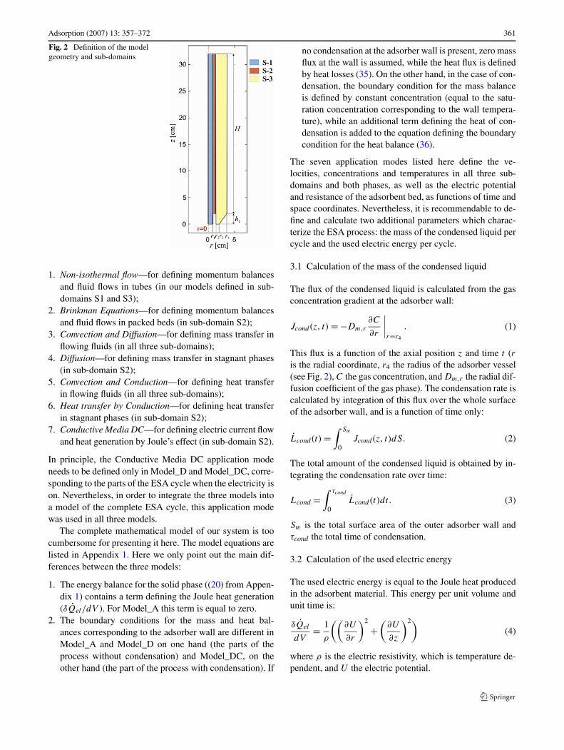
In order to reduce the model complexity, and using thefact that the adsorber is practically axially symmetrical, theComsol Multiphysics models were built in the axially sym-metrical 2D space. The model geometry, which is identicalfor all three models, is shown in Fig. 2. As can be seen fromthis figure, the model is defined for only one half of theadsorber, and the other half is axially symmetrical. In thatway, the number of the needed mesh elements is reduced tohalf, which dramatically reduces the computational time. InFig. 2, we also define the main adsorber dimensions and thesub-domains. Based on the structure of the adsorber, threesub-domains are defined (Fig. 2):

• S1—the central tube;• S2—the adsorbent bed;• S3—the annular space between the cartridge and the outer

adsorber wall.

In the Comsol Multiphysics working environment, themodel equations can be defined by choosing the appropriateapplication modes from a menu. The following applicationmodes were used in our models:

Adsorption (2007) 13: 357–372 361

Fig. 2 Definition of the modelgeometry and sub-domains

1. Non-isothermal flow—for defining momentum balancesand fluid flows in tubes (in our models defined in sub-domains S1 and S3);

2. Brinkman Equations—for defining momentum balancesand fluid flows in packed beds (in sub-domain S2);

3. Convection and Diffusion—for defining mass transfer inflowing fluids (in all three sub-domains);

4. Diffusion—for defining mass transfer in stagnant phases(in sub-domain S2);

5. Convection and Conduction—for defining heat transferin flowing fluids (in all three sub-domains);

6. Heat transfer by Conduction—for defining heat transferin stagnant phases (in sub-domain S2);

7. Conductive Media DC—for defining electric current flowand heat generation by Joule’s effect (in sub-domain S2).

In principle, the Conductive Media DC application modeneeds to be defined only in Model_D and Model_DC, corre-sponding to the parts of the ESA cycle when the electricity ison. Nevertheless, in order to integrate the three models intoa model of the complete ESA cycle, this application modewas used in all three models.

The complete mathematical model of our system is toocumbersome for presenting it here. The model equations arelisted in Appendix 1. Here we only point out the main dif-ferences between the three models:

1. The energy balance for the solid phase ((20) from Appen-dix 1) contains a term defining the Joule heat generation(δQel/dV ). For Model_A this term is equal to zero.

2. The boundary conditions for the mass and heat bal-ances corresponding to the adsorber wall are different inModel_A and Model_D on one hand (the parts of theprocess without condensation) and Model_DC, on theother hand (the part of the process with condensation). If

no condensation at the adsorber wall is present, zero massflux at the wall is assumed, while the heat flux is definedby heat losses (35). On the other hand, in the case of con-densation, the boundary condition for the mass balanceis defined by constant concentration (equal to the satu-ration concentration corresponding to the wall tempera-ture), while an additional term defining the heat of con-densation is added to the equation defining the boundarycondition for the heat balance (36).

The seven application modes listed here define the ve-locities, concentrations and temperatures in all three sub-domains and both phases, as well as the electric potentialand resistance of the adsorbent bed, as functions of time andspace coordinates. Nevertheless, it is recommendable to de-fine and calculate two additional parameters which charac-terize the ESA process: the mass of the condensed liquid percycle and the used electric energy per cycle.

3.1 Calculation of the mass of the condensed liquid

The flux of the condensed liquid is calculated from the gasconcentration gradient at the adsorber wall:

Jcond(z, t) = −Dm,r

∂C

∂r

∣∣∣∣r=r4

. (1)

This flux is a function of the axial position z and time t (ris the radial coordinate, r4 the radius of the adsorber vessel(see Fig. 2), C the gas concentration, and Dm,r the radial dif-fusion coefficient of the gas phase). The condensation rate iscalculated by integration of this flux over the whole surfaceof the adsorber wall, and is a function of time only:

Lcond(t) =∫ Sw

0Jcond(z, t)dS. (2)

The total amount of the condensed liquid is obtained by in-tegrating the condensation rate over time:

Lcond =∫ τcond

0Lcond(t)dt. (3)

Sw is the total surface area of the outer adsorber wall andτcond the total time of condensation.

3.2 Calculation of the used electric energy

The used electric energy is equal to the Joule heat producedin the adsorbent material. This energy per unit volume andunit time is:

δQel

dV= 1

ρ

((∂U

∂r

)2

+(

∂U

∂z

)2)

(4)

where ρ is the electric resistivity, which is temperature de-pendent, and U the electric potential.

362 Adsorption (2007) 13: 357–372

The used electric power is obtained by integration overthe adsorbent bed volume:

Qel(t) =∫ z=H

z=0

∫ r=r3

r=r2

r1

ρ

((∂U

∂r

)2

+(

∂U

∂z

)2)

2πdr dz

(5)

and the total used energy during desorption, by integrationover time:

Qel =∫ τdes

0Qel(t)dt. (6)

τdes is the total desorption time and H , r2 and r3 the adsorberdimensions defined in Fig. 2.

4 Model of the complete ESA cycle

In order to simulate the complete ESA cycle, the threeComsol Multiphysics models defined in the previous sec-tion have to be run in a sequence, with automatic switch-ing from one model to the next one when certain predefinedconditions are met. The following switches need to be per-formed:

• Switching from Model_A to Model_D. This switch corre-sponds to the end of adsorption and start of a new desorp-tion step. It is performed automatically when the outletconcentration reaches a certain predefined breakthroughvalue Cbreak. The outlet concentration is obtained as theaverage value across the outlet, although the simulationresults showed that the gas concentration across the out-let is nearly uniform.

• Switching from Model_D to Model_DC. This switch isperformed at the moment when the gas concentration atthe adsorber wall becomes equal to the saturation concen-tration corresponding to the wall temperature Csat, result-ing with the start of condensation. The saturation concen-tration is calculated using the Wagner equation (Reid etal. 1987). The simulations show that condensation prac-tically starts at the same time at the whole surface of theouter wall of the adsorber.

• Switching from Model_DC to Model_A. This switch de-fines the end of desorption and start of a new adsorptionpart of the cycle. It is performed when the maximal tem-perature in the adsorbent bed reaches certain predefinedvalue Tsw , which should not be exceeded, and the elec-tricity is switched off. The modeled ESA cycle does notassume a cooling step between the end of heating and startof the new adsorption step (Sullivan 2003).

Although in principle different Comsol Multiphysics mod-els can be run consecutively, automatic switching fromone model to another, by checking whether certain con-ditions are met, is not possible in Comsol Multiphysics.

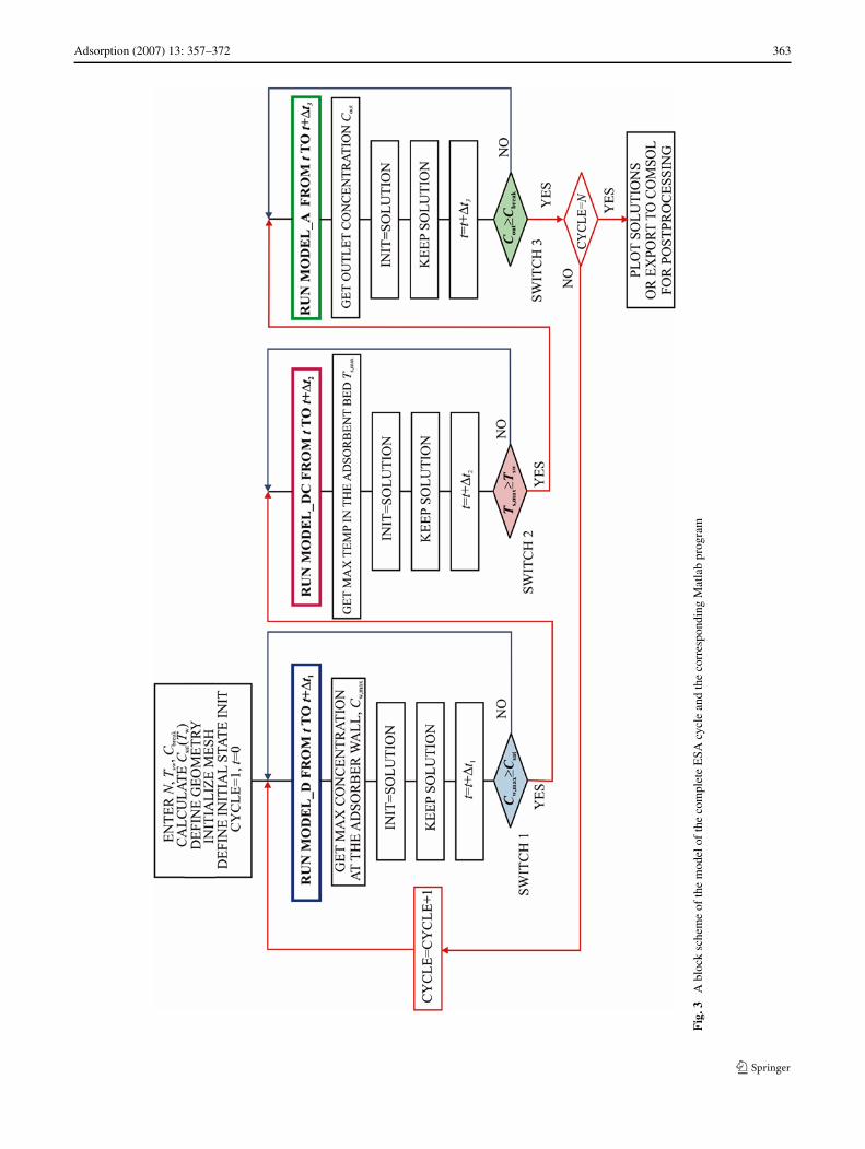
The problem was solved by using the coherence of Com-sol Multiphysics and Matlab. All three Comsol Multi-physics models were saved as Matlab m-files and thenintegrated into one Matlab model, defining the completecycle. The structure of this integral model is shown inFig. 3.

In this figure, as well as in our program, the cycle isstarted with the desorption step, with an equilibrium ini-tial state in which the temperatures of both phases are equal(and equal to the temperature of the environment) and theadsorbent bed is assumed to be saturated, in equilibriumwith the inlet gas concentration during the adsorption step.This sequence was chosen because it results with muchfaster establishing of the cyclic steady-state (in only 2–3cycles), compared to the case when the process is startedwith the adsorption step, from an initially clean adsorbentbed.

In order to enable integration of the models, the sameapplication modes have to be defined in all three ComsolMultiphysics models, in exactly the same sequence. Also,the model geometry and the mesh have to be identical in allthree models. Actually, in our integral model the model seg-ments corresponding to geometry definition and mesh ini-tialization are defined only once (Fig. 3).

5 Solution of the models and some simulation results

5.1 Used mesh, solvers and parameters

Comsol Multiphysics software is based on the finite elementmethod for solving systems of coupled partial differentialequations (PDEs) (Comsol AB 2005). The first step in thesolution procedure is generation of the mesh for the finiteelement method. In our simulations we used a normal den-sity mesh, with 568 mesh elements, which ensured a goodcompromise between high accuracy of the solution, withoutserious convergence problems on one, and moderate com-putational times, on the other hand.

The finite element method is actually a method of dis-cretization which approximates the PDEs by large sets ofordinary differential equations (ODEs). The software of-fers a choice of different solvers for solving the resultingsets of ODEs. In our simulations we used the direct UMF-PACK solver (Comsol AB 2005), which showed good re-sults.

The models of the presented system were solved and usedfor simulation of separate stages and of the complete ESAcycles, for the following adsorber dimensions:

• Length of the cartridge: 30 cm• Radius of the central tube of the cartridge: 0.95 cm• Thickness of the adsorbent bed: 0.55 cm• Radius of the adsorber vessel: 3.5 cm.

Adsorption (2007) 13: 357–372 363

Fig

.3A

bloc

ksc

hem

eof

the

mod

elof

the

com

plet

eE

SAcy

cle

and

the

corr

espo

ndin

gM

atla

bpr

ogra

m

364 Adsorption (2007) 13: 357–372

The physical parameters in our models correspond to thefollowing adsorption system (Sullivan 2003):

• Adsorbent: American Kynol ACC-5092-20 (activatedcarbon fiber cloth material)

• Adsorbate: methyl ethyl ketone (MEK)• Carrier gas: nitrogen.

The simulations were performed for different switch tem-peratures, breakthrough concentrations, supply voltagesand gas flow-rates during the adsorption and desorptionhalf-cycles. The inlet concentration during adsorption wasequal to the initial gas concentration (in all simulations0.001 mol/mol). The initial, inlet gas and ambient tempera-tures were all equal (293.15 K).

The complete list of the model parameters, with their de-finitions and the numerical values used in the simulations isgiven in Appendix 2.

The software offers a variety of graphical representationof the data. We will give a small portion of the simulationresults, as illustration.

5.2 Simulation results for separate stages

The developed Comsol Multiphysics models were first usedfor simulation of adsorption on a previously clean adsorbentand desorption from a previously saturated adsorbent bed.As a result, the gas velocities, pressures, concentrations andtemperatures in all parts of the adsorber are simulated. Hereare some of these results.

In Fig. 4, the gas velocities in all three subdomains arepresented in vector form. The velocity profiles in the systemare established very fast (during the first 2–3 seconds). After

that, the velocities change somewhat, owing to the changeof the gas temperature and concentration, but the changes ofthe velocity profiles are not significant. The results shownin Fig. 4 correspond to adsorption and t = 7000 s when theadsorption is complete. Very similar picture of the velocityprofiles is obtained for desorption. Figure 4 shows that in thecentral tube and in the annular space the gas flows mainlyin the axial direction, and through the adsorbent bed in theradial direction.

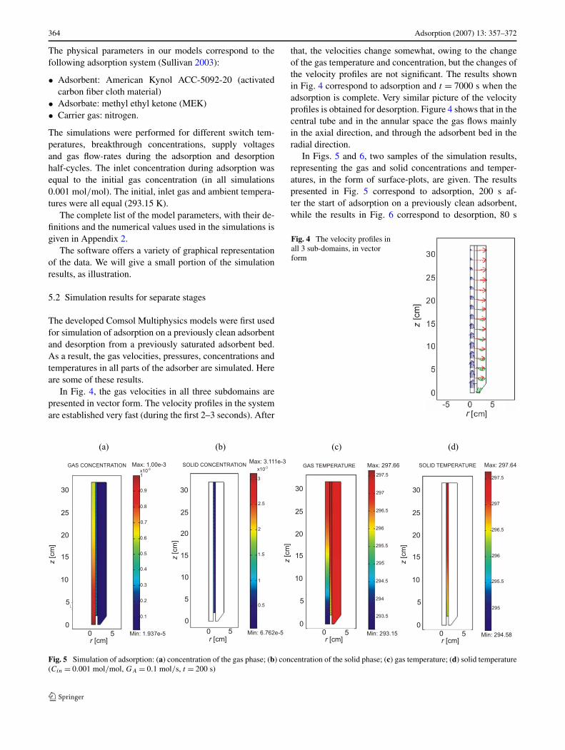
In Figs. 5 and 6, two samples of the simulation results,representing the gas and solid concentrations and temper-atures, in the form of surface-plots, are given. The resultspresented in Fig. 5 correspond to adsorption, 200 s af-ter the start of adsorption on a previously clean adsorbent,while the results in Fig. 6 correspond to desorption, 80 s

Fig. 4 The velocity profiles inall 3 sub-domains, in vectorform

Fig. 5 Simulation of adsorption: (a) concentration of the gas phase; (b) concentration of the solid phase; (c) gas temperature; (d) solid temperature(Cin = 0.001 mol/mol, GA = 0.1 mol/s, t = 200 s)

Adsorption (2007) 13: 357–372 365

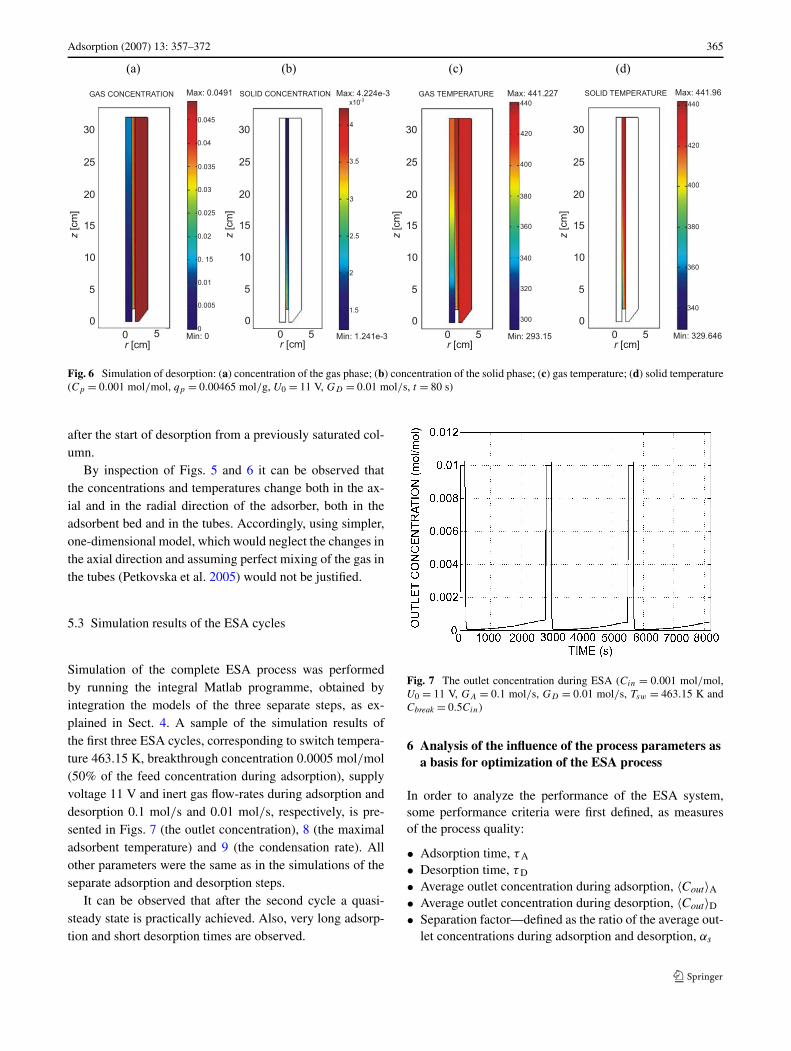
Fig. 6 Simulation of desorption: (a) concentration of the gas phase; (b) concentration of the solid phase; (c) gas temperature; (d) solid temperature(Cp = 0.001 mol/mol, qp = 0.00465 mol/g, U0 = 11 V, GD = 0.01 mol/s, t = 80 s)

after the start of desorption from a previously saturated col-umn.

By inspection of Figs. 5 and 6 it can be observed thatthe concentrations and temperatures change both in the ax-ial and in the radial direction of the adsorber, both in theadsorbent bed and in the tubes. Accordingly, using simpler,one-dimensional model, which would neglect the changes inthe axial direction and assuming perfect mixing of the gas inthe tubes (Petkovska et al. 2005) would not be justified.

5.3 Simulation results of the ESA cycles

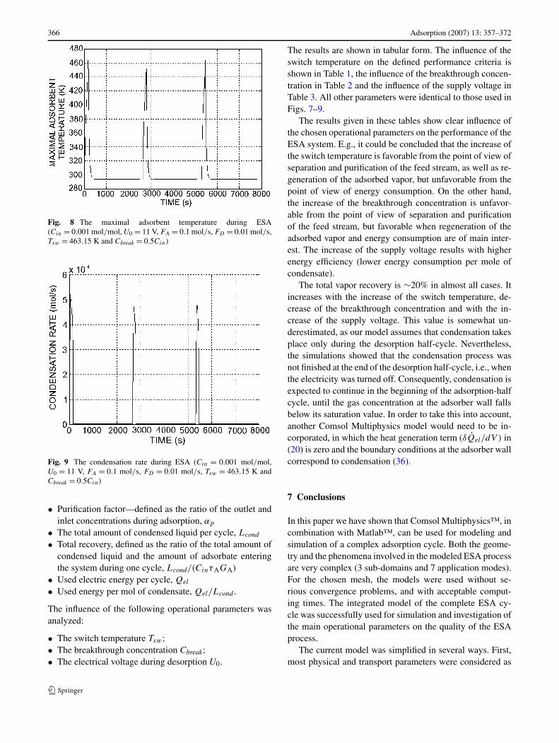
Simulation of the complete ESA process was performedby running the integral Matlab programme, obtained byintegration the models of the three separate steps, as ex-plained in Sect. 4. A sample of the simulation results ofthe first three ESA cycles, corresponding to switch tempera-ture 463.15 K, breakthrough concentration 0.0005 mol/mol(50% of the feed concentration during adsorption), supplyvoltage 11 V and inert gas flow-rates during adsorption anddesorption 0.1 mol/s and 0.01 mol/s, respectively, is pre-sented in Figs. 7 (the outlet concentration), 8 (the maximaladsorbent temperature) and 9 (the condensation rate). Allother parameters were the same as in the simulations of theseparate adsorption and desorption steps.

It can be observed that after the second cycle a quasi-steady state is practically achieved. Also, very long adsorp-tion and short desorption times are observed.

Fig. 7 The outlet concentration during ESA (Cin = 0.001 mol/mol,U0 = 11 V, GA = 0.1 mol/s, GD = 0.01 mol/s, Tsw = 463.15 K andCbreak = 0.5Cin)

6 Analysis of the influence of the process parameters asa basis for optimization of the ESA process

In order to analyze the performance of the ESA system,some performance criteria were first defined, as measuresof the process quality:

• Adsorption time, τA

• Desorption time, τD

• Average outlet concentration during adsorption, 〈Cout〉A

• Average outlet concentration during desorption, 〈Cout〉D

• Separation factor—defined as the ratio of the average out-let concentrations during adsorption and desorption, αs

366 Adsorption (2007) 13: 357–372

Fig. 8 The maximal adsorbent temperature during ESA(Cin = 0.001 mol/mol, U0 = 11 V, FA = 0.1 mol/s, FD = 0.01 mol/s,Tsw = 463.15 K and Cbreak = 0.5Cin)

Fig. 9 The condensation rate during ESA (Cin = 0.001 mol/mol,U0 = 11 V, FA = 0.1 mol/s, FD = 0.01 mol/s, Tsw = 463.15 K andCbreak = 0.5Cin)

• Purification factor—defined as the ratio of the outlet andinlet concentrations during adsorption, αp

• The total amount of condensed liquid per cycle, Lcond

• Total recovery, defined as the ratio of the total amount ofcondensed liquid and the amount of adsorbate enteringthe system during one cycle, Lcond/(CinτAGA)

• Used electric energy per cycle, Qel

• Used energy per mol of condensate, Qel/Lcond .

The influence of the following operational parameters wasanalyzed:

• The switch temperature Tsw;• The breakthrough concentration Cbreak;• The electrical voltage during desorption U0.

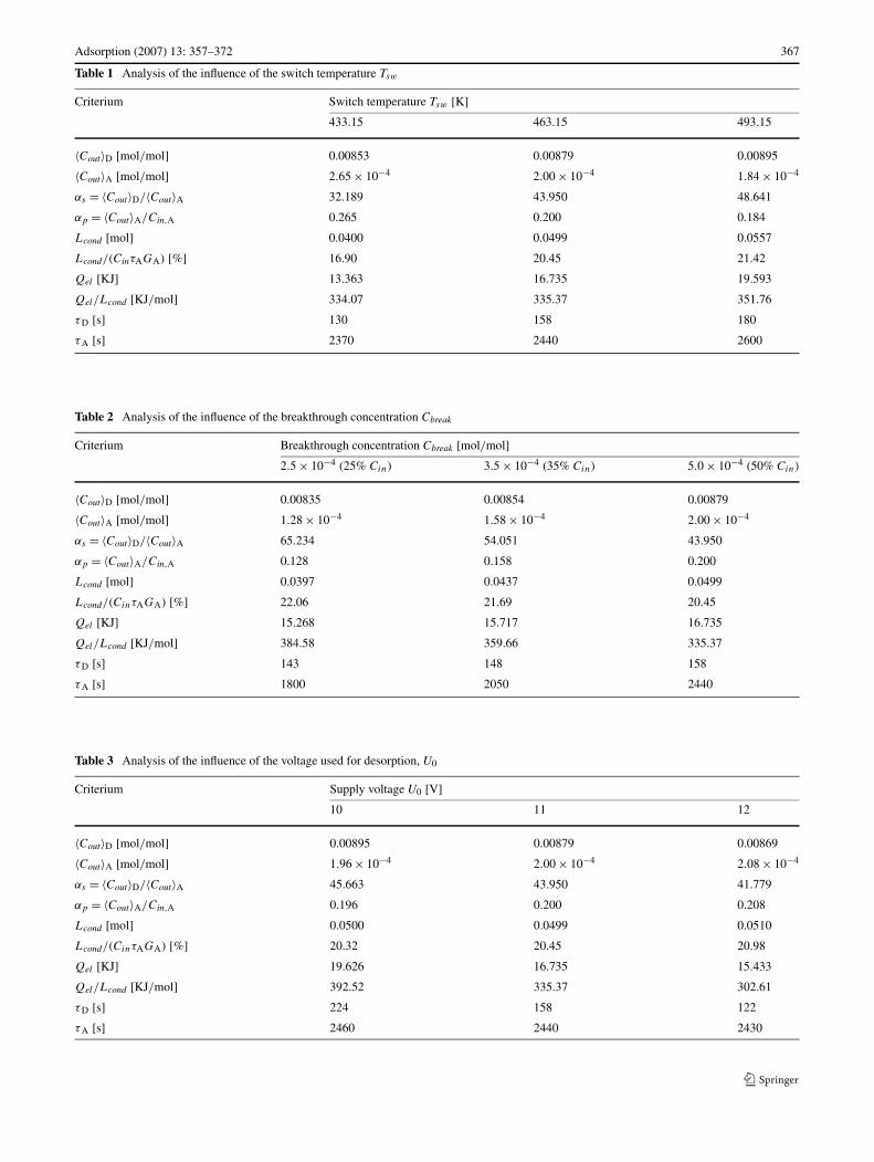
The results are shown in tabular form. The influence of theswitch temperature on the defined performance criteria isshown in Table 1, the influence of the breakthrough concen-tration in Table 2 and the influence of the supply voltage inTable 3. All other parameters were identical to those used inFigs. 7–9.

The results given in these tables show clear influence ofthe chosen operational parameters on the performance of theESA system. E.g., it could be concluded that the increase ofthe switch temperature is favorable from the point of view ofseparation and purification of the feed stream, as well as re-generation of the adsorbed vapor, but unfavorable from thepoint of view of energy consumption. On the other hand,the increase of the breakthrough concentration is unfavor-able from the point of view of separation and purificationof the feed stream, but favorable when regeneration of theadsorbed vapor and energy consumption are of main inter-est. The increase of the supply voltage results with higherenergy efficiency (lower energy consumption per mole ofcondensate).

The total vapor recovery is ∼20% in almost all cases. Itincreases with the increase of the switch temperature, de-crease of the breakthrough concentration and with the in-crease of the supply voltage. This value is somewhat un-derestimated, as our model assumes that condensation takesplace only during the desorption half-cycle. Nevertheless,the simulations showed that the condensation process wasnot finished at the end of the desorption half-cycle, i.e., whenthe electricity was turned off. Consequently, condensation isexpected to continue in the beginning of the adsorption-halfcycle, until the gas concentration at the adsorber wall fallsbelow its saturation value. In order to take this into account,another Comsol Multiphysics model would need to be in-corporated, in which the heat generation term (δQel/dV ) in(20) is zero and the boundary conditions at the adsorber wallcorrespond to condensation (36).

7 Conclusions

In this paper we have shown that Comsol Multiphysics™, incombination with Matlab™, can be used for modeling andsimulation of a complex adsorption cycle. Both the geome-try and the phenomena involved in the modeled ESA processare very complex (3 sub-domains and 7 application modes).For the chosen mesh, the models were used without se-rious convergence problems, and with acceptable comput-ing times. The integrated model of the complete ESA cy-cle was successfully used for simulation and investigation ofthe main operational parameters on the quality of the ESAprocess.

The current model was simplified in several ways. First,most physical and transport parameters were considered as

Adsorption (2007) 13: 357–372 367

Table 1 Analysis of the influence of the switch temperature Tsw

Criterium Switch temperature Tsw [K]

433.15 463.15 493.15

〈Cout〉D [mol/mol] 0.00853 0.00879 0.00895

〈Cout〉A [mol/mol] 2.65 × 10−4 2.00 × 10−4 1.84 × 10−4

αs = 〈Cout〉D/〈Cout〉A 32.189 43.950 48.641

αp = 〈Cout〉A/Cin,A 0.265 0.200 0.184

Lcond [mol] 0.0400 0.0499 0.0557

Lcond/(CinτAGA) [%] 16.90 20.45 21.42

Qel [KJ] 13.363 16.735 19.593

Qel/Lcond [KJ/mol] 334.07 335.37 351.76

τD [s] 130 158 180

τA [s] 2370 2440 2600

Table 2 Analysis of the influence of the breakthrough concentration Cbreak

Criterium Breakthrough concentration Cbreak [mol/mol]

2.5 × 10−4 (25% Cin) 3.5 × 10−4 (35% Cin) 5.0 × 10−4 (50% Cin)

〈Cout〉D [mol/mol] 0.00835 0.00854 0.00879

〈Cout〉A [mol/mol] 1.28 × 10−4 1.58 × 10−4 2.00 × 10−4

αs = 〈Cout〉D/〈Cout〉A 65.234 54.051 43.950

αp = 〈Cout〉A/Cin,A 0.128 0.158 0.200

Lcond [mol] 0.0397 0.0437 0.0499

Lcond/(CinτAGA) [%] 22.06 21.69 20.45

Qel [KJ] 15.268 15.717 16.735

Qel/Lcond [KJ/mol] 384.58 359.66 335.37

τD [s] 143 148 158

τA [s] 1800 2050 2440

Table 3 Analysis of the influence of the voltage used for desorption, U0

Criterium Supply voltage U0 [V]

10 11 12

〈Cout〉D [mol/mol] 0.00895 0.00879 0.00869

〈Cout〉A [mol/mol] 1.96 × 10−4 2.00 × 10−4 2.08 × 10−4

αs = 〈Cout〉D/〈Cout〉A 45.663 43.950 41.779

αp = 〈Cout〉A/Cin,A 0.196 0.200 0.208

Lcond [mol] 0.0500 0.0499 0.0510

Lcond/(CinτAGA) [%] 20.32 20.45 20.98

Qel [KJ] 19.626 16.735 15.433

Qel/Lcond [KJ/mol] 392.52 335.37 302.61

τD [s] 224 158 122

τA [s] 2460 2440 2430

368 Adsorption (2007) 13: 357–372

constants, although, strictly speaking they change with thevelocity and/or composition and/or temperature, and con-sequently, with time and space coordinates. These rela-tions can be included in the model, although that would in-crease its complexity and introduce additional coupling ofthe equations. Second, the heat capacity and resistance ofthe adsorber wall were neglected, although, they generallyshould be taken into account. In order to do that, anothersub-domain has to be added, with one application mode(Heat transfer by conduction) defined in it. Also, the heattransfer by radiation was not taken into account, althoughfor the temperatures of the adsorbent bed during desorption,it should probably not be neglected.

In the next generation of multiphysics models of the ESAsystem we are planning to gradually upgrade the complexityby taking into account all these aspects.

Multiphysics modeling of more complex adsorbers withtwo and four cartridges is also in progress.

Acknowledgements Effort sponsored by the Air Force Office ofScientific Research, Air Force Material Command, USAF, undergrant number FA8655-04-1-3053. This work was also partly sup-ported by the Serbian Ministry of Science in the frame of ProjectNo. 142014G.

Appendix 1: The model equations

8.1 Momentum balances and continuity equations for thegas phase

For the central tube and the annular space between the car-tridge and the adsorber wall (sub-domains S-1 and S-3):

rρg

∂u

∂t+ ∇

[

−2rμ∂u

∂r− rμ

(∂u

∂z+ ∂v

∂r

)]

= −(

r

(

ρg

(

u∂u

∂r+ v

∂u

∂z

)

+ ∂p

∂r

)

+ 2μu

r

)

, (7)

rρg

∂v

∂t+ ∇

[

−rμ

(∂v

∂r+ ∂u

∂z

)

− 2rμ∂v

∂z

]

= −r

(

ρg

(

u∂v

∂r+ v

∂v

∂z

)

+ ∂p

∂z

)

, (8)

−(

ρg

(

r

(∂u

∂r+ ∂v

∂z

)

+ u

)

+ ∂ρg

∂ru + ∂ρg

∂zv

)

= 0. (9)

For the adsorbent bed (sub-domain S-2):

rρg

∂u

∂t+ ∇

[

−2rμ∂u

∂r+

(

−rμ

(∂u

∂z+ ∂v

∂r

))]

= −(

r

(μ

ku + ∂p

∂r

)

+ 2μu

r

)

, (10)

rρg

∂v

∂t+ ∇

[

−rμ

(∂v

∂r+ ∂u

∂z

)

− 2rμ∂v

∂z

]

= −r

(μ

kv + ∂p

∂z

)

, (11)

−(

ρg

(

r

(∂u

∂r+ ∂v

∂z

)

+ u

)

+ ∂ρg

∂ru + ∂ρg

∂zv

)

= 0. (12)

The gas density is calculated as:

ρg = p

RgTg(1 + C), (13)

8.2 Heat balances for the gas phase

For the central tube and the annular space between the car-tridge and the adsorber wall (S-1 and S-3):

r∂

∂t

[

ρg(cpg + cpvC)Tg

] + ∇(

−rDhgt,r

∂Tg

∂r− rD

hgt,z

∂Tg

∂z

)

= −rρgcpvTg

(

u∂C

∂r+ v

∂C

∂z

)

− rρg(cpg + cpvC)u∂Tg

∂r

− rρg(cpg + cpvC)v∂Tg

∂z. (14)

For the adsorbent bed (S-2):

r∂

∂t

[

ρg(cpg + cpvC)Tg

]

+ ∇(

−rDhgt,r,b

∂Tg

∂r− rD

hgt,z,b

∂Tg

∂z

)

= r

(

hba(Ts − Tg) − ρgcpvTg

(

u∂C

∂r+ v

∂C

∂z

))

− rρg(cpg + cpvC)u∂Tg

∂r

− rρg(cpg + cpvC)v∂Tg

∂z. (15)

8.3 Adsorbate balances for the gas phase

For the central tube and the annular space between the car-tridge and the adsorber wall (S-1 and S-3):

r∂C

∂t+ ∇

(

−rDm,r

ρg

∂C

∂r− r

Dm,z

ρg

∂C

∂z

)

= −(

ru∂C

∂r+ rv

∂C

∂z

)

. (16)

For the adsorbent bed (S-2):

r∂C

∂t+ ∇

(

−rDm,r,b

ρg

∂C

∂r− r

Dm,z,b

ρg

∂C

∂z

)

= rkma

ρg

(C∗ − C) −(

ru∂C

∂r+ rv

∂C

∂z

)

. (17)

Adsorption (2007) 13: 357–372 369

8.4 Electric current balance for resistive heating (S-2)

∇(

−r1

ρ

∂U

∂r− r

1

ρ

∂U

∂z

)

= 0. (18)

Linear temperature dependence of the electric resistivity ofthe adsorbent material, which was obtained experimentallyfor ACFC adsorbent (Sullivan 2003) is used:

ρ = ρ0(1 + b(Ts − TR)). (19)

8.5 Heat balance for the solid phase within the adsorbentbed (S-2)

rρb

∂

∂t

[

(cps + cplq)Ts

] − ∇(

rDhst,r

∂Ts

∂r+ rDhs

t,z

∂Ts

∂z

)

= rδQel

dV+ rρb�Hads

∂q

∂t− rhba(Ts − Tg), (20)

δQel

dV= 1

ρ

((∂U

∂r

)2

+(

∂U

∂z

)2)

= 1

ρ0(1 + b(Ts − TR))

((∂U

∂r

)2

+(

∂U

∂z

)2)

. (21)

8.6 Adsorbate balance for the solid phase within theadsorbent bed (S-2)

ρb

∂q

∂t= kma(C − C∗). (22)

8.7 Equilibrium relation

Based on Dubinin–Radushkevich equation (Dubinin 1989),a relation between the equilibrium adsorbate concentrationin the gas phase C∗ and its concentration in the solid phaseq and temperature Ts is obtained:

C∗ = po

pexp

[

− E

RgTs

√

− ln

(MAq

ρAW0

)]

. (23)

Wagner equation (Reid et al. 1987) is used to calculate theadsorbate saturation pressure po, needed in (23):

ln

(po

pc

)

=(

V PAx + V PBx1.5 + V PCx3 + V PDx6

1 − x

)

,

x = 1 − (Ts/Tc). (24)

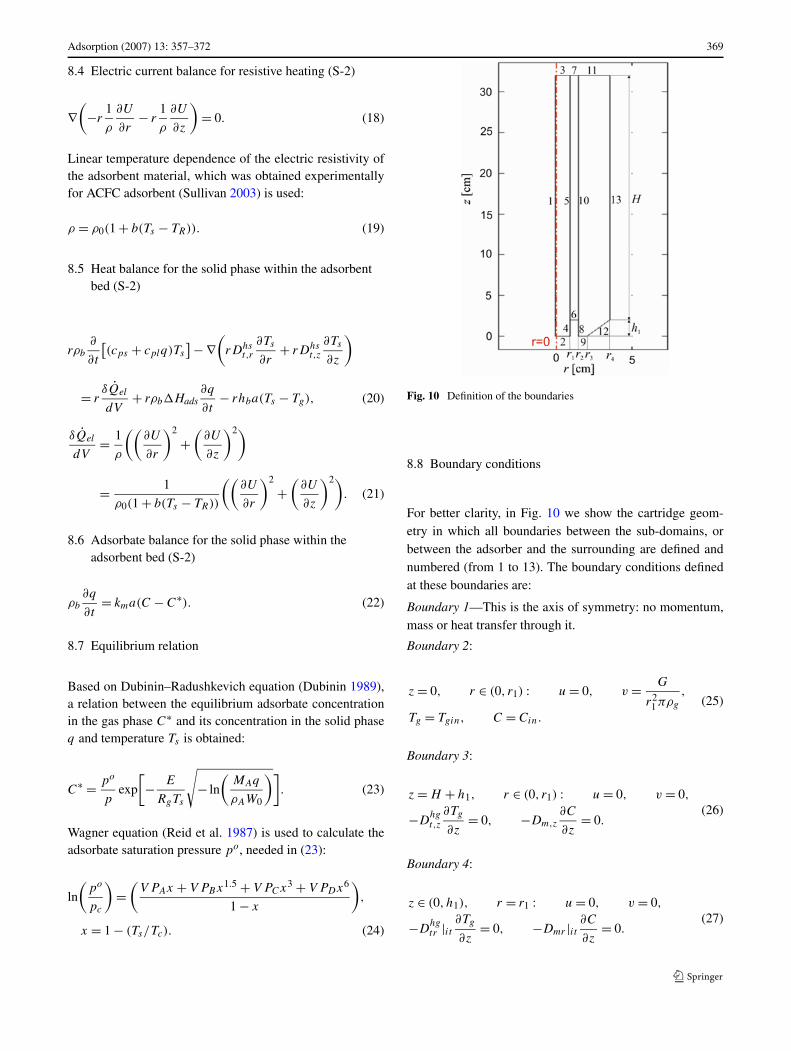
Fig. 10 Definition of the boundaries

8.8 Boundary conditions

For better clarity, in Fig. 10 we show the cartridge geom-etry in which all boundaries between the sub-domains, orbetween the adsorber and the surrounding are defined andnumbered (from 1 to 13). The boundary conditions definedat these boundaries are:

Boundary 1—This is the axis of symmetry: no momentum,mass or heat transfer through it.

Boundary 2:

z = 0, r ∈ (0, r1) : u = 0, v = G

r21πρg

,

Tg = Tgin, C = Cin.

(25)

Boundary 3:

z = H + h1, r ∈ (0, r1) : u = 0, v = 0,

−Dhgt,z

∂Tg

∂z= 0, −Dm,z

∂C

∂z= 0.

(26)

Boundary 4:

z ∈ (0, h1), r = r1 : u = 0, v = 0,

−Dhgtr |it ∂Tg

∂z= 0, −Dmr |it ∂C

∂z= 0.

(27)

370 Adsorption (2007) 13: 357–372

Boundary 5:

r = r1, z ∈ (h1, h1 + H) : p|ct = p|b,u|ct = u|b, v|ct = v|b,(

−Dhgt,r

∂Tg

∂r+ ρg(cpg + cpvC)uTg

)

ct

=(

−Dhgt,r,b

∂Tg

∂r+ ρg(cpg + cpvC)uTg

)

b

+ hs1(1 − εb)(Ts − Tg),

(

−Dm,r

∂C

∂r+ uC

)

ct

=(

−Dm,r,b

∂C

∂r+ uC

)

b

+ km1(1 − εb)(C∗ − C),

−Dhst,r

∂Ts

∂r= hs1(Tg − Ts), J = 0.

(28)

Boundary 6:

z = h1, r ∈ (r1, r2) : u = 0, v = 0,

−Dhgt,z,b

∂Tg

∂z= 0, −Dm,z,b

∂C

∂z= 0,

U = U0, −Dhstz

∂Ts

∂z= 0.

(29)

Boundary 7:

z = h1 + H, r ∈ (r1, r2) : u = 0, v = 0,

−Dhgt,z,b

∂Tg

∂z= 0, −Dm,z,b

∂C

∂z= 0,

U = 0, Dhstz

∂Ts

∂z= 0.

(30)

Boundary 8:

z ∈ (0, h1), r = r2 : u = 0, v = 0,

−Dhgt,r

∂Tg

∂z= 0, −Dm,r

∂C

∂z= 0.

(31)

Boundary 9:

z = 0, r ∈ (r2, r3) : p|as = pa,

−Dhgt,z

∂Tg

∂z= 0, −Dm,z

∂C

∂z= 0.

(32)

Boundary 10:

r = r2, z ∈ (h,h + H) : p|b = p|as,

u|b = u|ot , v|b = v|as,

(

−Dhgt,r,b

∂Tg

∂r+ ρg(cpg + cpvC)uTg

)

b

=(

−Dhgt,r

∂Tg

∂r+ ρg(cpg + cpvC)uTg

)

ot

+ hs2(1 − εb)(Ts − Tg),

(

−Dm,r,b

∂C

∂r+ uC

)

b

=(

−Dm,r

∂C

∂r+ uC

)

ot

+ km2(1 − εb)(C∗ − C),

J = 0, −Dhst,r

∂Ts

∂r= hs2(Tg − Ts).

(33)

Boundary 11:

z = h + H, r ∈ (r2, r4) : u = 0, v = 0,

−Dhgt,z

∂Tg

∂z= 0, −Dm,z

∂C

∂z= 0.

(34)

Boundaries 12 and 13—These boundaries correspond to theouter wall of the adsorber. The boundary conditions corre-sponding to this surface are different for the cases withoutand with condensation.

• For Model_A and Model_D (adsorption and desorptionwithout condensation):

r = r4, z ∈ (h,h + H) and r ∈ (r3, r4),

z ∈ (0, h) : u = 0, v = 0,

−Dm,r

∂C

∂z= 0, −D

hgt,r

∂Tg

∂r= hwg(Tg − Ta).

(35)

• For Model_DC (desorption with condensation):

r = r4, z ∈ (h,h + H) and

r ∈ (r3, r4), z ∈ (0, h) :u = 0, v = 0, C = Csat (Tw),

−Dhgt,r

∂Tg

∂r= −Dm,r

∂C

∂r(−�Hcond) + hwg(Tg − Ta).

(36)

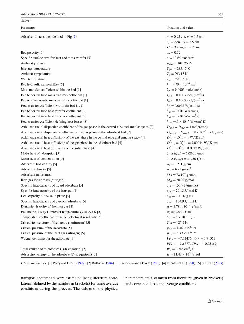
Appendix 2: Definitions and values of the modelparameters used for simulation

All transport coefficients and physical parameters used inthe models were considered as constants. The values of the

Adsorption (2007) 13: 357–372 371

Table 4

Parameter Notation and value

Adsorber dimensions (defined in Fig. 2) r1 = 0.95 cm, r2 = 1.5 cm

r3 = 2 cm, r4 = 3.5 cm

H = 30 cm, h1 = 2 cm

Bed porosity [5] εb = 0.72

Specific surface area for heat and mass transfer [5] a = 13.65 cm2/cm3

Ambient pressure patm = 101325 Pa

Inlet gas temperature Tgin = 293.15 K

Ambient temperature Ta = 293.15 K

Wall temperature Tw = 293.15 K

Bed hydraulic permeability [5] k = 4.59 × 10−6 cm2

Mass transfer coefficient within the bed [1] km = 0.0003 mol/(cm2 s)

Bed to central tube mass transfer coefficient [1] km1 = 0.0003 mol/(cm2 s)

Bed to annular tube mass transfer coefficient [1] km2 = 0.0003 mol/(cm2 s)

Heat transfer coefficient within the bed [1, 2] hb = 0.0055 W/(cm2 s)

Bed to central tube heat transfer coefficient [3] hs1 = 0.001 W/(cm2 s)

Bed to central tube heat transfer coefficient [3] hs2 = 0.001 W/(cm2 s)

Heat transfer coefficient defining heat losses [3] hwg = 5 × 10−5 W/(cm2 K)

Axial and radial dispersion coefficient of the gas phase in the central tube and annular space [2] Dm,z = Dm,r = 1 mol/(cm s)

Axial and radial dispersion coefficient of the gas phase in the adsorbent bed [2] Dm,z,b = Dm,z,b = 8 × 10−5 mol/(cm s)

Axial and radial heat diffusivity of the gas phase in the central tube and annular space [4] Dhgt,z = D

hgt,r = 1 W/(K cm)

Axial and radial heat diffusivity of the gas phase in the adsorbent bed [4] Dhgt,z,b = D

hgt,r,b = 0.00014 W/(K cm)

Axial and radial heat diffusivity of the solid phase [4] Dhst,r = Dhs

t,r = 0.0012 W/(cm K)

Molar heat of adsorption [5] (−�Hads) = 66200 J/mol

Molar heat of condensation [5] (−�Hcond) = 31230 J/mol

Adsorbent bed density [5] ρb = 0.221 g/cm3

Adsorbate density [5] ρA = 0.81 g/cm3

Adsorbate molar mass MA = 72.107 g/mol

Inert gas molar mass (nitrogen) MB = 28.02 g/mol

Specific heat capacity of liquid adsorbate [5] cpl = 157.9 J/(mol K)

Specific heat capacity of the inert gas [5] cpg = 29.13 J/(mol K)

Heat capacity of the solid phase [5] cps = 0.71 J/(g K)

Specific heat capacity of gaseous adsorbate [5] cpv = 100.9 J/(mol K)

Dynamic viscosity of the inert gas [1] μ = 1.78 × 10−4 g/cm/s

Electric resistivity at referent temperature TR = 293 K [5] ρ0 = 0.202 � cm

Temperature coefficient of the bed electrical resistivity [5] b = −2 × 10−3 1/K

Critical temperature of the inert gas (nitrogen) [5] TcB = 126.2 K

Critical pressure of the adsorbate [5] pcA = 4.26 × 106 Pa

Critical pressure of the inert gas (nitrogen) [5] pcB = 3.39 × 106 Pa

Wagner constants for the adsorbate [5] VPA = −7.71476, VPB = 1.71061

VPC = −3.6877, VPD = −0.75169

Total volume of micropores (D-R equation) [5] W0 = 0.748 cm3/g

Adsorption energy of the adsorbate (D-R equation) [5] E = 14.43 × 103 J/mol

Literature sources: [1] Perry and Green (1997), [2] Ruthven (1984), [3] Incropera and DeWitt (1996), [4] Fuentes et al. (1998), [5] Sullivan (2003)

transport coefficients were estimated using literature corre-lations (defined by the number in brackets) for some averageconditions during the process. The values of the physical

parameters are also taken from literature (given in brackets)

and correspond to some average conditions.

372 Adsorption (2007) 13: 357–372

References

Azou, A., Martin, G., Le Cloirec, P.: Improvement of a closed cycle forremoval and recovery of dilute gases—application to dry cleaningindustry. Environ. Technol. 14, 471–478 (1993)

Baudu, M., Le Cloirec, P., Martin, G.: La regeneration par echauf-fement intrinseque de charbons actifs utilises pour le traitementd’air. Environ. Technol. 13, 423–435 (1992)

Bathen, D.: Gasphasen—Adsorption in der Umwelttechnik—Stand derTechnik und Perspektiven. Chemie Ingenieur Technik 74, 209–216 (2002)

Bathen, D., Schmidt-Traub, H., Stube, J.: Experimenteller Vorgleichverschiedener thermischer Desorptionsverfahren zur Losungsmit-tel ruckgewinnung. Chemie Ingenieur Technik 69, 132–134(1997)

Comsol AB: Comsol Documentation, Comsol Multiphysics UsersGuide (2005)

Dubinin, M.M.: Fundamentals of the theory of adsorption in microp-ores of carbon adsorbents: characteristics of their adsorption prop-erties and microporous structures. Carbon 27, 457–467 (1989)

Fabuss, B.M., Dubois, W.H.: Carbon adsorption-electrodesorptionprocess. In: 63rd Annual Meeting of the Air Pollution ControlAssociation, St. Louis, MO (1970)

Fuentes, J., Pironti, F., Lopez de Ramos, A.L.: Effective thermal con-ductivity in a radial-flow packed-bed reactor. Int. J. Thermophys.19, 781–792 (1998)

Incropera, F.P., DeWitt, D.P.: Fundamentals of Heat and Mass Transfer.Wiley, New York (1996)

Lordgooei, M., Carmichael, K.R., Kelly, T.W., Rood, M.J., Larson,S.M.: Activated carbon cloth adsorption—cryogenic system to re-cover toxic volatile organic compound. Gas Sep. Purif. 10, 123–130 (1996)

Luo, L., Ramirez, D., Rood, M., Grevillot, G., Hay, J., Thurston, D.:Adsorption and electrothermal desorption of organic vapors usingactivated carbon adsorbents with novel morphologies. Carbon 44,2715–2723 (2006)

Moon, S.H., Shim, J.W.: A novel process for CO2/CH4 gas separationon activated carbon fibers—electric swing adsorption. J. ColloidInterface Sci. 298, 523–528 (2006)

Petkovska, M., et al.: Temperature-swing gas separation with elec-trothermal desorption step. Sep. Sci. Technol. 26, 425–444 (1991)

Petkovska, M., Antov, D., Sullivan, P.: Electrothermal desorption in anannular-radial flow-ACFC adsorber-mathematical modeling. Ad-sorption 11(1 Suppl.), 585–590 (2005)

Petkovska, M., Mitrovic, M.: Microscopic modeling of electrothermaldesorption. Chem. Eng. J. Biochem. Eng. J. 53, 157–165 (1994a)

Petkovska, M., Mitrovic, M.: One-dimensional, non-adiabatic, mi-croscopic model of electrothermal desorption process dynamics.Chem. Eng. Res. Des. 72, 713–722 (1994b)

Perry, R.H., Green, D.W.: Perry’s Chemical Engineer’s Handbook, 7thedn. McGraw–Hill, New York (1997)

Reid, R.C., Prausnitz, J.M., Poling, B.: The Properties of Gases & Liq-uids. McGraw–Hill, New York (1987)

Rood, M., et al.: Selective sorption and desorption of gases with elec-trically heated activated carbon fiber cloth element. US PatentNo. 6,346,936 B1 (2002)

Ruthven, D.M.: Principles of Adsorption and Adsorption Processes.Wiley, New York (1984)

Snyder, J.D., Leesch, J.G.: Methyl bromide recovery on activated car-bon with repeated adsorption and electrothermal regeneration.Ind. Eng. Chem. Res. 40, 2925–2933 (2001)

Subrenat, A., Le Cloirec, P.: Industrial application of adsorption ontoactivated carbon cloths and electro-thermal regeneration. J. Envi-ron. Eng. 130, 249–257 (2004)

Subrenat, A.S., Le Cloirec, P.A.: Volatile organic compound (VOC)removal by adsorption onto activated carbon fiber cloth andelectrothermal desorption: An industrial application. Chem. Eng.Commun. 193, 478–486 (2006)

Sullivan, P.: Organic vapor recovery using activated carbon fiber clothand electrothermal desorption. Ph.D. thesis, University of Illinoisat Urbana-Champaign (2003)

Sullivan, P.D., Rood, M.J., Hay, K.J., Qi, S.: Adsorption and elec-trothermal desorption of hazardous organic vapors. J. Environ.Eng. 127, 217–223 (2001)

Sullivan, P.D., Rood, M.J., Grevillot, G., Wander, J.D., Hay, K.J.: Acti-vated carbon fiber cloth electrothermal swing adsorption system.Environ. Sci. Technol. 38, 4865–4877 (2004a)

Sullivan, P.D., Rood, M.J., Dombrowski, K.D., Hay, K.J.: Capture oforganic vapors using adsorption and electrothermal regeneration.J. Environ. Eng. 130, 258–267 (2004b)

Sushchev, S.V., Shumyatskii, Y.I., Alekhina, M.B.: Steady-state tem-perature and adsorption distributions in a resistance-heated gran-ular activated-charcoal bed. Theor. Found. Chem. Eng. 36, 141–144 (2002)

Yu, F.D., Luo, L.A., Grevillot, G.: Adsorption isotherms of VOCs ontoan activated carbon monolith: experimental measurement and cor-relation with different models. J. Chem. Eng. Data 47, 467–473(2002)

Yu, F.D., Luo, L., Grevillot, G.: Electrothermal swing adsorption oftoluene on an activated carbon monolith: experiments and para-metric theoretical study. Chem. Eng. Proc. 46, 70–81 (2007)