Multiple Brake Orbits and Homoclinics in Riemannian Manifolds

Digital Object Identifier (DOI) 10.1007/s00205-010-0371-1Arch. Rational Mech. Anal. 200 (2011) 691–724

Multiple Brake Orbits and Homoclinicsin Riemannian Manifolds

Roberto Giambò, Fabio Giannoni & Paolo Piccione

Communicated by P. Rabinowitz

Abstract

Let (M, g) be a complete Riemannian manifold,� ⊂ M an open subset whoseclosure is homeomorphic to an annulus. We prove that if ∂� is smooth and it sat-isfies a strong concavity assumption, then there are at least two distinct geodesicsin � = � ∪ ∂� starting orthogonally to one connected component of ∂� andarriving orthogonally onto the other one. Using the results given in Giambò et al.(Adv Differ Equ 10:931–960, 2005), we then obtain a proof of the existence oftwo distinct homoclinic orbits for an autonomous Lagrangian system emanatingfrom a nondegenerate maximum point of the potential energy, and a proof of theexistence of two distinct brake orbits for a class of Hamiltonian systems. Under afurther symmetry assumption, the result is improved by showing the existence of atleast dim(M) pairs of geometrically distinct geodesics as above, brake orbits andhomoclinic orbits. In our proof we shall use recent deformation results proved inGiambò et al. (Nonlinear Anal Ser A: Theory Methods Appl 73:290–337, 2010).

1. Introduction

In this paper we will use a non-smooth version of the Ljusternik–Schnirelmantheory to prove the existence of multiple orthogonal geodesic chords in Riemannianmanifolds with boundary. This fact, together with the results in [7], gives a multi-plicity result for homoclinics and brake orbits of a class of Hamiltonian systems.Let us recall a few basic facts and notations from [7].

1.1. Geodesics in Riemannian manifolds with boundary

Let (M, g) be a smooth (that is, of class C2) Riemannian manifold withdim(M) = m � 2, let dist denote the distance function on M induced by g;the symbol ∇ will denote the covariant derivative of the Levi–Civita connection of

692 Roberto Giambò, Fabio Giannoni & Paolo Piccione

g, as well as the gradient differential operator for smooth maps on M . The Hes-sian H f (q) of a smooth map f : M → R at a point q ∈ M is the symmetricbilinear form H f (q)(v,w) = g ((∇v∇ f )(q), w) for all v,w ∈ Tq M ; equivalently,

H f (q)(v, v) = d2

ds2

∣∣s=0 f (γ (s)), where γ : ]−ε, ε[ → M is the unique (affinely

parameterized) geodesic in M with γ (0) = q and γ (0) = v. We will denote by Ddt

the covariant derivative along a curve, in such a way that Ddt γ = 0 is the equation

of the geodesics. A basic reference on the background material for Riemanniangeometry is [5].

Let � ⊂ M be an open subset; � = � ∪ ∂� will denote its closure. Thereare several notions of convexity and concavity in Riemannian geometry, extendingthe usual ones for subsets of the Euclidean space R

m . In this paper we will usea somewhat strong concavity assumption for compact subsets of M that we willcall “strong concavity” below, and which is stable by C2-small perturbations of theboundary. Let us first recall the following (see also [2,12]):

Definition 1. � is said to be convex if every geodesic γ : [a, b] → � whose end-points γ (a) and γ (b) are in � has an image entirely contained in �. Likewise, �is said to be concave if its complement M \� is convex.

If ∂� is a smooth embedded submanifold of M , let IIn(x) : Tx (∂�)×Tx (∂�) →R denote the second fundamental form of ∂� in the normal direction n ∈ Tx (∂�)

⊥.Recall that IIn(x) is a symmetric bilinear form on Tx (∂�) defined by:

IIn(x)(v,w) = g(∇vW, n), v,w ∈ Tx (∂�),

where W is any local extension of w to a smooth vector field along ∂�.

Remark 1. Assume a given smooth function φ : M → R with the property that� = φ−1 (]−∞, 0[) and ∂� = φ−1(0), with dφ = 0 on ∂�.1 The followingequality between the Hessian Hφ and the second fundamental form2 of ∂� holds:

Hφ(x)(v, v) = −II∇φ(x)(x)(v, v), x ∈ ∂�, v ∈ Tx (∂�); (1)

Namely, if x ∈ ∂�, v ∈ Tx (∂�) and V is a local extension around x of v to a vectorfield which is tangent to ∂�, then v (g(∇φ, V )) = 0 on ∂�, and thus:

Hφ(x)(v, v) = v (g(∇φ, V ))− g(∇φ,∇vV ) = −II∇φ(x)(x)(v, v).

For convenience, we will fix throughout the paper a function φ as above. Weobserve that, although the second fundamental form is defined intrinsically, thereis no canonical choice for the function φ describing the boundary of � as above.

Definition 2. We will say that that� is strongly concave if IIn(x) is negative definitefor all x ∈ ∂� and all inward pointing normal directions n.

1 For example one can choose φ such that |φ(q)| = dist(q, ∂�) for all q in a (closed)neighborhood of ∂�.

2 Observe that, with our definition of φ, then ∇φ is a normal vector to ∂� pointingoutwards from �.

Multiple Brake Orbits and Homoclinics in Riemannian Manifolds 693

Observe that if � is strongly concave, geodesics starting tangentially to ∂� moveinside �.

Remark 2. Strong concavity is evidently a C2-open condition. Then, by (1), if �is compact, we deduce the existence of δ0 > 0 such that Hφ(x)(v, v) < 0 for allx ∈ φ−1 ([−δ0, δ0]) and for all v ∈ Tx M , v = 0, such that g (∇φ(x), v) = 0.

A simple contradiction argument based on Taylor expansion shows that, underthe above condition, it is ∇φ(q) = 0, for all q ∈ φ−1([−δ0, δ0]).Remark 3. Let δ0 be as above. The strong concavity condition gives us the follow-ing property of geodesics, that will be used systematically throughout the paper:

for any geodesic γ : [a, b]→� with φ(γ (a))=φ(γ (b))=0and φ(γ (s))<0 for all s ∈ ]a, b[, there exists s ∈ ]a, b[ such that φ (γ (s))<−δ0.

(2)

This property is proved easily by looking at the minimum point of the map s →φ(γ (s)).

The main objects of our study are geodesics in M having images in� and withendpoints orthogonal to ∂�, that will be called orthogonal geodesic chords:

Definition 3. A geodesic γ : [a, b] → M is called a geodesic chord in � ifγ (]a, b[) ⊂ � and γ (a), γ (b) ∈ ∂�; by a weak geodesic chord we will mean ageodesic γ : [a, b] → M with image in� and endpoints γ (a), γ (b) ∈ ∂� and suchthat γ (s0) ∈ ∂� for some s0 ∈]a, b[. A (weak) geodesic chord is called orthog-onal if γ (a+) ∈ (Tγ (a)∂�)⊥ and γ (b−) ∈ (Tγ (b)∂�)⊥, where γ ( · ±) denote thelateral derivatives (see Fig. 1). An orthogonal geodesic chord in�whose endpointsbelong to distinct connected components of ∂�will be called a crossing orthogonalgeodesic chord in �.

For brevity, we will write OGC for “orthogonal geodesic chord” and WOGCfor “weak orthogonal geodesic chord”. Although the general class of weak orthog-onal geodesic chords are perfectly acceptable solutions of our initial geometricalproblem, our suggested construction of a variational setup works well only in asituation where one can exclude a priori the existence in � of orthogonal geodesicchords γ : [a, b] → � for which there exists s0 ∈ ]a, b[ such that γ (s0) ∈ ∂�.

One does not lose generality in assuming that there are no such WOGCs in �by recalling the following result from [7]:

Proposition 1. Let � ⊂ M be an open set whose boundary ∂� is smooth andcompact and with � strongly concave. Assume that there are only a finite numberof (crossing) orthogonal geodesic chords in �. Then, there exists an open subset�′ ⊂ � with the following properties:

1. �′ is diffeomorphic to � and it has smooth boundary;2. �′ is strongly concave;


Fig. 1. A weak orthogonal geodesic chord (WOGC) γ in � (above), and a crossing OGC(below)

3. the number of (crossing) OGCs in �′ is less than or equal to the number of(crossing) OGCs in �;

4. there are no (crossing) WOGCs in �′.Proof. See [7, Proposition 2.6]

In the central result of this paper we will give a lower estimate on the numberof distinct orthogonal geodesic chords; we recall here some results in this directionavailable in the literature. In [3], Bos proved that if ∂� is smooth, � convex andhomeomorphic to the m-dimensional disk, then there are at least m distinct OGCsfor �. Such a result is a generalization of a classical result by Ljusternik andSchnirelman (see [16]), where the same result was proven for convex subsets ofR

m endowed with the Euclidean metric. Bos’s result was used in [14] to prove amultiplicity result for brake orbits under a certain “non-resonance condition”. In[11] the authors have studied the problem of how the multiplicity of OGCs on amanifold with convex boundary is related to the topology of the domain; in par-ticular, they prove that if � is homeomorphic to an annulus there are at least twoOGCs.

By an m-dimensional annulus we mean a topological space homeomorphic totopological product S

m−1 × [0, 1], that can be thought as the subset of Rm :

{

p ∈ Rm : 1 � |p| � 2

};Motivated by the study of a certain class of Hamiltonian systems (see Subsec-

tion 1.2), in this paper we will study the case of sets with strongly concave boundary.Our central result is the following:


Theorem 1. Let� be an open subset of M with smooth boundary ∂�, such that�is strongly concave and homeomorphic to an annulus. Then, there are at least twogeometrically distinct3 crossing orthogonal geodesic chords in �.

Remark 4. By Proposition 1, it suffices to prove Theorem 1 under the furtherassumption that:

there are no crossing WOGCs in �. (3)

For this reason, from now on we shall assume (3).

Multiplicity of OGCs in the case of compact manifolds having convex bound-ary is typically proven by applying a curve-shortening argument. From an abstractviewpoint, the curve-shortening process can be seen as the construction of a flowin the space of paths, along whose trajectories the length or energy functional isdecreasing.

In this paper we will follow the same procedure, with the difference that boththe space of paths and the shortening flow have to be defined appropriately.

Shortening a curve having its image in a closed convex subset� of a Riemann-ian manifold produces another curve in�; in this sense, we think of the shorteningflow as being “inward pushing” in the convex case. Opposite to the convex case,the shortening flow in the concave case will be “outwards pushing”, and this factrequires that one should consider only those portions of a curve which remain inside� when it is stretched outwards. This type of analysis has been carried out in [10],and we shall employ here many of the results proved in [10].

The concavity condition plays a central role in the variational setup of our con-struction. “Variational criticality” relative to the energy functional will be definedin terms of “outwards pushing” infinitesimal deformations of the path space (seeDefinition 5). The class of variationally critical portions properly contains the setof portions consisting of crossing OGCs; such curves will be defined as “geometri-cally critical” paths (see Definition 4). In order to construct the shortening flow, anaccurate analysis of all possible variationally critical paths is required (Section 4),and the concavity condition will guarantee that such paths are well behaved (seeLemma 3, Propositions 3 and 4). Using these properties, we will able to move awayfrom critical portions which are not crossing OGCs.

Once a reasonable classification of variationally critical points is obtained, theshortening flow is constructed by techniques which are typical of the pseudo-gradient vector field approach. A technical description of the abstract minimaxframework that we will use is given in Subsection 1.3.

Note that the estimate in Theorem 1 cannot be improved; namely, for all m � 2there are strictly concave subsets of R

m that are diffeomorphic to the m-dimensionalannulus, and admitting precisely two orthogonal geodesic chords:

3 By geometrically distinct curves we mean curves having distinct images as subsets of�.


Example 1. Let ψ : R+ → R

+ be a smooth function chosen in such a way thatthe annulus

�0 = {

x ∈ Rm : 1 � |x | � 2

}

is strongly concave relative to the conformally flat metric on Rm :

g(x) = ψ (|x |) · g0(x),

g0 being the Euclidean metric on Rm . For instance, strong concavity of �0 is

guaranteed when the conformal factor ψ satisfies:12ψ

′(1)+ ψ(1) > 0, and ψ ′(2)+ ψ(2) < 0.

For ε ∈ Rm , |ε| < 1, set:

�ε = {

x ∈ Rm : 1 < |x |, |x − ε| < 2

}

.

We claim that, for |ε| small enough, the following situation occurs:

1. �ε is strongly concave;2. there are only two distinct OGCs in �ε,

relative to the metric g.Assertion (1) is obvious, since strong concavity is an open condition and �0 is

strongly concave. As to assertion 2, the argument goes as follows. Denote by D1and D2 the two connected components of ∂�ε:

D1 = {

x ∈ Rm : |x | = 1

}

, D2 = {

x ∈ Rm : |x − ε| = 2

};since g is radially symmetric, the geodesics starting orthogonally to D1 have imagescontained on a half-line through the origin of R

m . Those arriving orthogonally toD2 must be parallel to the vector ε, hence there are only two of them ( γ1 and γ2 inFig. 2).

On the other hand, if |ε| is small enough, there are no orthogonal geodesicchords in�ε having both endpoints on D2. So, for ε = 0, all the geodesics startingorthogonally to D2 arrive orthogonally, and in particular transversally, to D1. SinceD2 is compact, and transversality is an open condition, it also holds for |ε| smallenough, which proves our claim.

Example 1 can be visualized as follows. Consider the manifold � obtained byremoving two small open disks around the north and the south pole of a roundsphere (see Fig. 3). This manifold is evidently strongly concave. The two disks canbe obtained by cutting the sphere with two planes; if the planes are not parallel,then there are precisely two orthogonal geodesic chords in �.

It is not hard to prove the existence of at least one orthogonal crossing geodesicchord in �, which is given by a distance minimizing curve between the two con-nected components D1 and D2 of ∂�. On the other hand, if one drops the concavityassumption, then a second orthogonal geodesic chord may not exist.

Example 2. The assumption of concavity in Theorem 1 cannot be omitted; an exam-ple of � diffeomorphic to a two-dimensional annulus having only one orthogonalgeodesic chord is represented in Fig. 4. The example is obtained as a C0-smallperturbation of a region which is bounded by two non-concentric circles.


Fig. 2. The two orthogonal geodesic chords γ1 and γ2 of Example 1

orthogonal geodesic chords

Fig. 3. The sphere with two convex discs removed. The boundaries of the discs lie in non-parallel planes, so that there are only two orthogonal geodesic chords

1.2. Brake and homoclinic orbits of Hamiltonian systems

The result of Theorem 1 can be applied to prove a multiplicity result for brakeorbits and homoclinic orbits, as follows.

Let p = (pi ), q = (qi ) be coordinates on R2m , and let us consider a natural

Hamiltonian function H ∈ C2(

R2m,R

)

, that is, a function of the form

H(p, q) = 1

2

m∑

i, j=1

ai j (q)pi p j + V (q), (4)


Fig. 4. The shaded region is a subset of the Euclidean plane diffeomorphic to a two-dimensional annulus with only one orthogonal geodesic chord γ that realizes the minimumdistance between the two connected components of ∂�

where V ∈ C2 (Rm,R) and A(q) = (

ai j (q))

is a positive definite quadratic formon R

m :

m∑

i, j=1

ai j (q)pi p j � ν(q)|q|2

for some continuous function ν : Rm → R

+ and for all (p, q) ∈ R2m .

The corresponding Hamiltonian system is:

⎧

⎪⎪⎨

⎪⎪⎩

p = −∂H

∂q

q = ∂H

∂p,

(5)

where the dot denotes differentiation with respect to time.For all q ∈ R

m , denote by L (q) : Rm → R

m the linear isomorphism whosematrix with respect to the canonical basis is

(

ai j (q))

, the inverse of(

ai j (q))

. It iseasily seen that, if (p, q) is a solution of class C1 of (5), then q is actually a mapof class C2 and

p = L (q)q. (6)

With a slight abuse of language, we will say that a C2-curve q : I → Rm (I interval

in R) is a solution of (5) if (p, q) is a solution of (5), where p is given by (6).Since the system (5) is autonomous, that is, time independent, then the functionH is constant along each solution and it represents the total energy of the solu-tion of the dynamical system. A large amount of literature exists concerning thestudy of periodic solutions of autonomous Hamiltonian systems having energy Hprescribed (see for instance [15] and the references therein).


We will be concerned with a special kind of periodic solutions of (5), calledbrake orbits. A brake orbit for the system (5) is a non-constant periodic solutionR � t → (p(t), q(t)) ∈ R

2m of class C2 with the property that p(0) = p(T ) = 0for some T > 0. Since H is even in the variable p, a brake orbit (p, q) is 2T -peri-odic, with p odd and q even about t = 0 and about t = T . Clearly, if E is theenergy of a brake orbit (p, q), then V (q(0)) = V (q(T )) = E .

The link between solutions of brake orbits and orthogonal geodesic chords isobtained in [7, Theorem 5.9]. Using this theorem and Theorem 1, we immediatelyget the following:

Theorem 2. Let H ∈ C2(

R2m,R

)

be a natural Hamiltonian function as in (4),E ∈ R and

�E = V −1 (]−∞, E[) .

Assume that dV (x) = 0 for all x ∈ ∂�E and that �E is homeomorphic to anm-dimensional annulus. Then, the Hamiltonian system (5) has at least two geomet-rically distinct brake orbits having energy E and endpoints in different connectedcomponents of V −1(E).

Let us now go back to our Riemannian manifold (M, g) and assume that we aregiven a map V ∈ C2 (M,R); the corresponding second order Hamiltonian systemis the equation:

Ddt q + ∇V (q) = 0. (7)

When M = Rm and g is the Riemannian metric

g = 1

2

m∑

i, j=1

ai j (x) dxi dx j , (8)

where the coefficients ai j are as above, then equation (7) is equivalent to (5), in thesense that x is a solution of (7) if and only if the pair q = x and p = L (x)x is asolution of (5).

Let x0 ∈ M be a critical point of V , that is, such that ∇V (x0) = 0. A homoclinicorbit for the system (7) emanating from x0 is a solution q ∈ C2 (R,M) of (7) suchthat:

limt→−∞ q(t) = lim

t→+∞ q(t) = x0, (9)

limt→−∞ q(t) = lim

t→+∞ q(t) = 0. (10)

Surprisingly enough, multiplicity results for homoclinic orbits of (7) have beenestablished mostly in the non-autonomous periodic case (that is, when the functionV depends periodically on t), using variational methods (see for instance Refer-ences [4,13,21,22]). The autonomous case is somewhat harder to treat, and, to theknowledge of the authors, the only results available in the literature are:


– Reference [1], where it is considered a superquadratic potential in Rm satisfying

a pinching property, a superquadraticity condition, and a suitable assumption onthe second derivative;

– Reference [18], where the results of [1] are improved by removing the superqua-draticity condition and the assumption on the second derivative;

– Reference [20], where the author considers the case of a potential in Rm periodic

in all variables;– Reference [25], where it is considered a small perturbation of a radial potential.

As a further application of Theorem 1 and [7, Theorem 5.19], we have the followingtheorem, which gives a generalization of the results in [1,18,25]:

Theorem 3. Let (M, g) be a Riemannian manifold, V ∈ C2 (M,R) and let x0 ∈ Mbe a nondegenerate maximum point of V , with V (x0) = E. Assume that:

(a) V −1 (]−∞, E[) ∪ {x0} is homeomorphic to an open ball of Rm;

(b) dV (x) = 0 for all x ∈ V −1(E) \ {x0}.Then, there are at least two geometrically distinct homoclinic orbits for the system(7) emanating from x0 and reaching V −1(E) \ {x0}.It is not hard to produce examples of non-existence of homoclinics emanating froma nondegenerate saddle point of the potential V .

Finally, we consider the case of orthogonal geodesic chords in an annulus undera further central symmetry assumption. We will say that a subset A of a Riemannianmanifold (M, g) is centrally symmetric around the point x0 ∈ M if there existsan isometry I : M → M with I 2 = Id whose unique fixed point is x0 and suchthat I (A) = A. Observe that if γ : [a, b] → M is a geodesic, then I ◦ γ is alsoa geodesic in (M, g), and if γ is orthogonal at the endpoints at some hypersurface ⊂ M , then I ◦ γ is orthogonal at the endpoints to the hypersurface I (). If(M, g) is centrally symmetric around x0, a map f : M → R is said to be centrallysymmetric around x0 if f ◦ I = f , where I is the central isometry relative to x0.

Theorem 4. Under the hypotheses of Theorem 1, assume further that� is centrallysymmetric around a point y0 ∈ M \ �. Suppose that there isn’t any WOGC in �.Then there are at least m crossing orthogonal geodesic chords γ1, . . . , γm in �such that each γi is geometrically distinct from γ j and I ◦ γ j , ∀i = j .

In Proposition 1, we observe that if � is centrally symmetric, the open set �′can also be constructed centrally symmetric.

Accordingly, using [7, Theorem 5.9 and Theorem 5.19], we get similar multi-plicity results for brake orbits and for homoclinic orbits under a central symmetryassumption.

Theorem 5. Under the assumptions of Theorem 2, assume further that the func-tions ai j and V are centrally symmetric around some point y0 ∈ V −1 (]−∞, E]).Then there are at least m brake orbits γ1, . . . , γm of energy E for the Hamiltoniansystem (5), having extreme points in different connected components of V −1(E)and such that each γi is geometrically distinct from γ j and I ◦ γ j , ∀i = j .


Theorem 6. Under the assumptions of Theorem 3, if (M, g) is centrally symmetricrelative to x0 and the map V is also centrally symmetric around x0, then there areat least m homoclinic orbits γ1, . . . γm for the system (7) emanating from x0 andsuch that each γi is geometrically distinct from γ j and I ◦ γ j , ∀i = j .

The above results were announced in [8,9].

1.3. Abstract Ljusternik–Schnirelman theory

The main technique for proving Theorems 1 and 4 is a suitable non-smoothversion of the minimax theory of Ljusternik and Schnirelman. Let us recall that,given a topological space X and a subspace Y ⊂ X , Y is said to be contractiblein X if the inclusion map i : Y → X is homotopic to a constant map, that is,if there exists a point x0 ∈ X and a continuous map H : Y × [0, 1] → X suchthat h(y, 0) = y and h(y, 1) = x0 for all y ∈ Y . The Ljusternik–Schnirelmancategory of Y in X , denoted by catX (Y ), is defined as the minimum number(possibly infinite) of subsets of X that are open and contractible in X , and whoseunion contains Y ; we set cat(X ) = catX (X ). It is not hard to prove that theLjusternik–Schnirelman category is homotopy invariant; moreover, the category ismonotonic increasing by inclusion, that is, catX (Y1) � catX (Y2) if Y1 ⊂ Y2.Observe that the Ljusternik–Schnirelman category cat(SN ) of the N -sphere S

N

equals 2, while the category of the real projective space cat(RP N ) equals N + 1(see [23]).

If f : X → R is a C1 function on the complete Banach manifold X which isbounded from below and which satisfies suitable compactness assumptions (Palais– Smale), then f possesses at least cat(X ) distinct critical points (see for instance[17,24]).

The problem of orthogonal geodesic chords in a strongly concave domain� ofa Riemannian manifold M cannot be cast in a standard smooth variational context,due mainly to the fact that the classical shortening flow on curves in � with end-points on the boundary does not leave such a set invariant. In order to overcomethis problem, our strategy will be to reproduce the “ingredients” of the classicalsmooth theory in a suitable non-smooth context. More precisely, we will use thefollowing objects:

– a metric space M, that consists of curves having images in an open neighborhoodof� in M , and whose endpoints remain in different connected components of aneighborhood of ∂�;

– a compact subset C of M, homeomorphic to the (m − 1)-sphere;– a family H consisting of pairs (D, h), where D is a compact subset of C and

h : [0, 1] × D → M is a continuous map such that h(0, x) = x, ∀x ∈ D , andsatisfying suitable properties that will be listed in Section 6;

– a functional F : H → R+.

A suitable notion of critical level can be defined for the functional F in sucha way that distinct critical levels determine distinct crossing orthogonal geodesicchords in �. The crucial point of the approach is the proof of two “deformation


lemmas” for the sublevels of F using the homotopies in H . The first deformationlemma (Proposition 8) basically tells us that compact subsets of a noncritical sub-level of F can be deformed by suitable elements of H into compact subsets of alower sublevel of F . The second deformation lemma (Proposition 9) says that asimilar deformation also exists for compact subsets of critical levels of F , providedthat a suitable neighborhood of the “critical set” is removed. The analogue of theclassical Palais–Smale condition in our framework can be found in [10].

Once this setup has been established, the proof of multiplicity of critical levelsof F is carried out along the lines of the classical Ljusternik–Schnirelman theory,as follows. For i = 1, 2, set:

�i = {

D ∈ C : catC(D) � i}

, (11)

and

ci = infD∈�i

(D ,h)∈H

F (D, h) (12)

Then, the following facts hold:

(a) ci > 0, and ci < +∞ for i = 1, 2;(b) c1 � c2, as it follows immediately from (12);(c) each ci is a critical level of F , by the First Deformation Lemma (Proposition 8);(d) The second Deformation Lemma (Proposition 9), allows us to choose a suit-

able closed subset W containing curves having pieces which are close to cross-ing OGCs, and satisfying the following property (see Proposition 10): for any(D, h) ∈ H , there exists an open contractible subset A of C such that h(1,D \A ) ⊂ M \ W . This will allow us to obtain that c1 < c2.

The argument above proves the existence of at least two distinct critical levels forF . A crucial point is that distinct critical levels produce geometrically distinctcrossing orthogonal geodesic chords (Proposition 2).

For the multiplicity result in the case with symmetry, the argument is similar.Observe that the symmetry assumption implies that the functional F is invariantby a Z2-action. In order to obtain m distinct critical points, it will suffice to showthat the above construction can be carried out in an equivariant way, using theLjusternik–Schnirelman category of the real projective space RPm−1.

1.4. The functional framework

Throughout the paper, (M, g) will denote a Riemannian manifold of class C2;all our constructions will be made in suitable (relatively) compact subsets of M .For this reason it will not be restrictive to assume, as we will, that (M, g) is com-plete. Furthermore, we will work mainly in open subsets � of M whose closure ishomeomorphic to an m-dimensional annulus. In order to simplify the expositionwe will assume that, indeed,� is embedded topologically in R

m , which will allowto use an auxiliary linear structure on a neighborhood of �. We will also assumethat � is strongly concave in M .


The symbol H1 ([a, b],Rm) will denote the Sobolev space of all absolutelycontinuous curves in R

m whose weak derivative is square integrable. Similarly,H1 ([a, b],M) will denote the infinite dimensional Hilbert manifold consistingof all absolutely continuous curves x : [a, b] → M such that ϕ ◦ x |[c,d] ∈H1([c, d],Rm) for all charts ϕ : U ⊂ M → R

m of M such that x ([c, d]) ⊂ U . ByH1

0 (]a, b[ ,Rm)we will denote the subset of H1 ([a, b],M)with x(a) = x(b) = 0.For A ⊂ R

m and a < b we set

H1 ([a, b], A) ={

x ∈ H1 ([a, b],Rm) : x(s)∈ A for all s ∈ [a, b]}

. (13)

The Hilbert space norm ‖ · ‖a,b of H1 ([a, b],Rm) (equivalent to the usual one)will be defined by

‖x‖a,b =(

‖x(a)‖2E + ∫ b

a ‖x(s)‖2E ds

2

)1/2

, (14)

where ‖ · ‖E is the Euclidean norm in Rm ; note that

‖x‖L∞([a,b],Rm ) � ‖x‖a,b. (15)

We shall also use the space H2,∞, which consists of differentiable curves withabsolutely continuous derivatives and having weak second derivatives in L∞.

Remark 5. In the development of our results, we will have to deal with curves xwith variable domain [a, b] ⊂ [0, 1]. In this situation, by H1-convergence of asequence xn : [an, bn] → M to a curve x : [a, b] → M we will mean that an tendsto a, bn tends to b and xn : [a, b] → M is H1-convergent to x in H1 ([a, b],M)as n → ∞, where xn is the unique affine reparameterization of x on the interval[a, b] (and similarly for H1-weak convergence and for uniform convergence).

Set ∂� = D1 ∪ D2, where D1 and D2 are the two connected components of ∂�.We set:

ρ0 = minx∈D1y∈D2

dist(x, y) > 0 (16)

and

K0 = maxQ∈φ−1(]−∞,δ0])

‖∇φ(Q)‖. (17)

Here dist and ‖·‖ are considered with respect to the metric g, φ fixed as in Remark 1and δ0 is given by Remark 2. We shall prove the existence of at least two geomet-rically distinct orthogonal geodesic chords x1 and x2 such that x1(0), x2(0) ∈ D1and x1(1), x2(1) ∈ D2.


Fig. 5. The dotted curves represent typical elements of the path space M

2. Path space and maximal intervals

Let φ be as in Remark 1 and δ0 be as in Remark 3. Since dφ(q) = 0 wheneverq ∈ φ−1([−δ0, δ0]), the gradient flow of φ gives a strong deformation retract ofthe “band” φ−1 ([−δ0, δ0]) onto φ−1(0) = ∂�. For i = 1, 2, let us denote by Di

the connected component of φ−1 ([0, δ0[) that contains Di , and set4:

M0 ={

x ∈ H1(

[0, 1], φ−1(]−∞, δ0[))

: x(0)∈ D1, x(1)∈ D2

}

, (18)

see Fig. 5. This is a subset of the Hilbert space H1 ([0, 1],Rm), and it will be to-pologized with the induced metric. We shall use flows in H1([0, 1],Rm) for whichM0 is invariant.

For all x ∈ M0, let J 0x and Jx denote the following collections of closed

subintervals of [0, 1]:J 0

x = {[a, b] ⊂ [0, 1] : x([a, b]) ⊂ �, x(a) ∈ D1, x(b)∈ D2}

, (19)

Jx ={

[a, b] ∈ J 0x : [a, b] is maximal

with respect to the property of belonging to J 0x

}

. (20)

The elements of J 0x will be called crossing intervals. We observe that Jx is

a finite non-empty set; namely, if x ∈ M and [a, b] ∈ Jx , then:

ρ0 � dist (x(a), x(b)) �∫ b

ag(x, x)

12 dt �

√b − a

(∫ b

ag(x, x) dt

)1/2

, (21)

4 Observe that curves in M run across � in a specific direction, that is, from D1 to D2.


that implies

b − a � ρ20

(∫ b

ag(x, x) dt

)−1

, (22)

hence the cardinality of Jx is less than or equal to the integer part of the quantityρ−2

0

∫ 10 g(x, x) dt .

Remark 6. It is immediate to verify the following semicontinuity property. Sup-pose xn → x in M, [a, b] ∈ Jx and [an, bn] ∈ Jxn with [an, bn] ∩ [a, b] = ∅ forall n. Then

a � lim infn→∞ an � lim sup

n→∞bn � b.

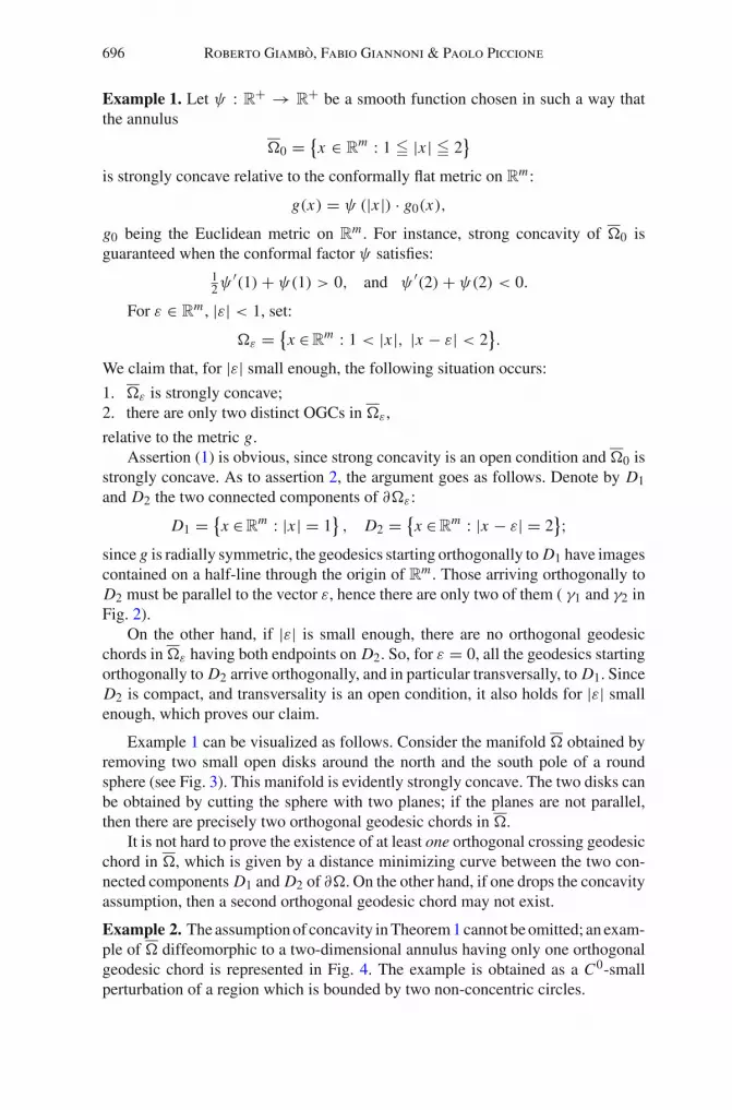
The following Lemma allows us to describe a subset C of M0 that will play acentral role in our construction.

Lemma 1. There exists a continuous map G : D1 → H1([0, 1],�) such that

1. G(A)(0) = A, for all A ∈ D1;2. G(A)(1) ∈ D2, for all A ∈ D1;3. A1 = A2 ⇒ G(A1)(1) = G(A2)(1);4. G(A)(s) ∈ � ∀A ∈ D1 ∀s ∈]0, 1[.Proof. Since � is homeomorphic to the annulus

A = {

q ∈ Rm : ‖q‖E ∈ [1, 2]} ,

we can consider a homeomorphism ψ :�→ A such that ψ(D1)={

q ∈ Rm : ‖q‖E

= 1}

and ψ(D2) = {q ∈ Rm : ‖q‖E = 2}. If ψ is a diffeomorphism we set

G(A)(s) = ψ−1((1 + s)ψ(A)) for any A ∈ D1.

(see Fig. 6).In general, if � is only homeomorphic to the annulus A, then the above defi-

nition produces curves which in principle are only continuous. In order to producecurves with an H1-regularity, we use a broken geodesic approximation argument.More precisely, if ψ is a homeomorphism as above, consider, for any A ∈ D1 thecurve

cA(s) = ψ−1 ((1 − s)ψ(A))

and the set

C′ = {cA : A ∈ D1}.Denote by �(�, g) the infimum of the injectivity radii of all points of � relativeto the metric g (see [5]). By the compactness of C′, there exists N0 ∈ N with theproperty that dist (cA(a), cA(b)) � �(�, g)whenever |a−b| � 1

N0for all cA ∈ C′.


Fig. 6. The dotted curves represent typical elements of the set C when � is the annulus

Finally, for all cA ∈ C′, denote by γA the broken geodesic obtained as a concatena-tion of the curves γk : [ k−1

N0, k

N0] → M given by the unique minimal geodesic in

(M, g) from cA(k−1N0) to cA(

kN0), k = 1, . . . , N0.

Note that, by compactness, N0 can be chosen so large as to have

φ(γA(s)) < δ0 for any s ∈ [0, 1], for any A ∈ D1.

Since the minimal geodesic in any convex normal neighborhood depends continu-ously (with respect to the C2-norm) on its endpoints, γA depends continuously byA in the H1-norm. Moreover γA satisfies (1), (2) and (3) of the statement.

Now, on the Riemannian manifold M , consider the flow η given by the solutionof the Cauchy problem

⎧

⎪⎨

⎪⎩

d

dτη(τ ) = −∇φ(η)

‖∇φ(η)‖2

η(0) = x ∈ {y ∈ M : −δ0 � φ(y) � δ0}

.

which is certainly well defined on φ−1([−δ0, δ0]), where ∇φ = 0. We can set

γ (A)(s) = η(max(0, φ (γA(s)) , γA(s)),

so that

γ (A)(s)∈� for any s ∈ [0, 1], for any A ∈ D1.

Since γ (A)(0) = A and γ (A)(1) ∈ D2, it is φ(γ (A)(0)) = φ(γ (A)(1)) = 0 andtherefore also γA satisfies (1), (2) and (3) of the statement. Finally,

G(A)(s) = η

(

s(1 − s)max

(

0,δ0

2+ φ(γA(s)

)

, γA(s)

)

,

is the desired map.


Note that J 0G(A) = JG(A) = {[0, 1]}. We set

C = {G(A) : A ∈ D1}. (23)

Obviously C is homeomorphic to Sm−1.

Define the following constant:

M0 = supx∈C

∫ 1

0g(x, x) dt; (24)

obviously, since C is compact and the integral in (24) is continuous in theH1-topology, then M0 < +∞. Using M0 we can finally define the functionalmetric space in which to set our minimax argument, setting

M ={

x ∈ M0 : 12

∫ b

ag(x, x) dt < M0 ∀ [a, b] ∈ Jx

}

. (25)

Observe that, by (22), if x ∈ M, the length of a crossing interval [a, b] is uniformlybounded away from zero since

b − a � ρ20

2M0. (26)

3. Geometrically critical values and variationally critical portions

In this section we will introduce two different notions of criticality for curvesin M.

Definition 4. A number c ∈ ]0,M0[ will be called a geometrically critical valueif there exists an OGC γ parameterized in [0, 1] such that 1

2

∫ 10 g(γ , γ ) dt = c.

A number which is not geometrically critical will be called geometrically regularvalue.

It is important to observe that, in view to obtaining multiplicity results, dis-tinct geometrically critical values yield geometrically distinct orthogonal geodesicchords:

Proposition 2. Let c1 = c2, c1, c2 > 0 be distinct geometrically critical valueswith corresponding OGC x1, x2. Then x1 ([0, 1]) = x2 ([0, 1]).Proof. The OGCs x1 and x2 are parameterized in the interval [0, 1]. Assume bycontradiction, x1([0, 1]) = x2([0, 1]). Since

xi (]0, 1[)⊂� for any i = 1, 2,

we have

{x1(0), x1(1)} = {x2(0), x2(1)}.


Up to reversing the orientation of x2, we can assume x1(0) = x2(0). Since x1 and x2are OGCs, x1(0) and x2(0) are parallel, but the condition c1 = c2 says that x1(0) =x2(0). Then there exists λ > 0, λ = 1 such that x2(0) = λx1(0) and therefore,by the uniqueness of the Cauchy problem for geodesics we have x2(s) = x1(λs).Up to exchange x1 with x2 we ca assume λ > 1. Since x2(

1λ) = x1(1) ∈ ∂�, the

transversality of x2(0) to ∂� implies the existence of s ∈] 1λ, 1] such that x2(s) ∈ �,

getting a contradiction.

A notion of criticality will now be given in terms of variational vector fields.For x ∈ M, let V +(x) denote the following closed convex cone of the spaceTx H1

([0, 1],RN)

:

V +(x) ={

V ∈ Tx H1(

[0, 1],RN)

: g (V (s),∇φ (x(s))) � 0 for x(s) ∈ ∂�}

;(27)

vector fields in V +(x) are interpreted as infinitesimal variations of x by curvesstretching “outwards” from the set �.

Definition 5. Let x ∈ M and [a, b] ⊂ [0, 1]; we say that x|[a,b] is aV +-variationally critical portion of x if x|[a,b] is not constant and if

∫ b

ag(

x, Ddt V

)

dt � 0, ∀ V ∈ V +(x). (28)

Similarly, for x ∈ M we define the cone:

V −(x) ={

V ∈ Tx H1(

[0, 1],RN)

: g (V (s),∇φ (x(s))) � 0 for x(s) ∈ ∂�}

,

(29)

and we give the following

Definition 6. Let x ∈ M and [a, b] ⊂ [0, 1]; we say that x|[a,b] is aV −-variationally critical portion of x if x|[a,b] is not constant and if

∫ b

ag(

x, Ddt V

)

dt � 0, ∀ V ∈ V −(x). (30)

The integrals in (28) and (30) give precisely the first variation of the geodesicaction functional in (M, g) along x|[a,b]. Hence, V +-variationally critical portionsare interpreted as those curves x|[a,b] whose geodesic energy is not decreased afterinfinitesimal variations by curves stretching outwards from the set �. The motiva-tion for using outwards pushing infinitesimal variations is due to the concavity of�. Indeed, in the convex case it is customary to use a curve shortening method in�, which can be seen as the use of a flow constructed by infinitesimal variations ofx in V −(x), keeping the endpoints of x on ∂�.

Flows obtained as integral flows of convex combinations of vector fields inV +(x) are, in a certain sense, the protagonists of our variational approach. How-ever we shall use also integral flows of convex combinations of vector fields in


V −(x) to avoid certain variationally critical portions that do not correspond toOGCs.

Clearly, we are interested in determining the existence of geometrically criticalvalues. In order to use a variational approach we will first have to take into consid-eration the more general class of V +-variationally critical portions. A central issuein our theory consists in studying the relations between V +-variationally criticalportions x|[a,b] and OGCs. From now on V +-variationally critical portions, will becalled simply variationally critical portions.

4. Classification of variationally critical portions

Let us now take a look at what variationally critical portions look like. In thefirst place, let us point out that regular variationally critical portions are OGCs. Inorder to prove this, the following two Lemmas are crucial. The first one is a simpleconsequence of Hölder’s inequality. The proof of the second one is found in [10].

Lemma 2. Let x ∈ M, [α, β] ⊂ [0, 1] and t ∈ [α, β] be such that x(α), x(β) ∈ ∂�and φ(x(t)) � −δ0. Then:

β − α � δ20

K 20

(∫ β

α

g(x, x) dt

)−1

.

Lemma 3. Let x ∈ M be fixed, and let [a, b] ∈ [0, 1] be such that x|[a,b] isa (non-constant) variationally critical portion of x, with x(a), x(b) ∈ ∂� andx ([a, b]) ⊂ �. Then:

1. x−1(∂�) ∩ [a, b] consists of a finite number of closed intervals and isolatedpoints;

2. x is constant on each connected component of x−1(∂�) ∩ [a, b];3. x|[a,b] is piecewise C2, and the discontinuities of x may occur only at points in

∂�;4. each C2 portion of x|[a,b] is a geodesic in �.5. inf{φ(x(s)) : s ∈ [a, b]} < −δ0.

Using the previous Lemmas, we can now prove the following:

Proposition 3. Assume that there are no crossing WOGCs in �. Let x ∈ M and[a, b] ∈ J 0

x be such that x|[a,b] is a variationally critical portion of x and suchthat the restriction of x to [a, b] is of class C1. Then, x|[a,b] is a crossing orthogonalgeodesic chord in � with x (]a, b[) ⊂ �, x(a) ∈ D1, x(b) ∈ D2.

Proof. C1-regularity, together with (1) and (2) of Lemma 3, show that x−1(∂�)∩[a, b] consists only of a finite number of isolated points. Then, by the C1 regularityon [a, b] and parts (3)–(4) of Lemma 3, x is a geodesic on the whole interval [a, b].Moreover an integration by parts argument shows that x(a) and x(b) are orthogonalto Tx(a)∂� and Tx(b)∂� respectively. Finally, since there is no crossing WOGC on�, x|[a,b] is a crossing OGC.


Ω

x(a) x([t , t ])

x(b)

x([t , t ])1 2

3 4

Fig. 7. Irregular critical portions of curves in M, with cusp intervals [t1, t2] and [t3, t4]

Variationally critical portions x|[a,b] of class C1 will be called regular vari-ationally critical portions; those critical portions that do not belong to this classwill be called irregular. Irregular variationally critical portions of curves x ∈ Mare further divided into two subclasses, described in the Proposition below, whoseproof can be obtained using Lemma 3 as it was used for the proof of Proposition 3.

Proposition 4. Assume that there are no WOGCs in�. Let x ∈ M and let [a, b] ∈J 0

x be such that x|[a,b] is an irregular variationally critical portion of x. Then,there exists a subinterval [α, β] ⊂ [a, b] such that x|[a,α] and x|[β,b] are constant(in ∂�), x(α+) ∈ Tx(α)(∂�)

⊥, x(β−) ∈ Tx(β)(∂�)⊥, and one of the two mutually

exclusive situations occurs:

1. there exists a finite number of intervals [t1, t2] ⊂ ]α, β[ such that x ([t1, t2]) ⊂∂� and that are maximal with respect to this property; moreover, x is constanton each such interval [t1, t2], and x(t−1 ) = x(t+2 );

2. x|[α,β] is a crossing OGC in �.

Irregular variationally critical portions in the class described in part (1) willbe called of the first type, those described in part (2) will be called of the secondtype. An interval [t1, t2] as in part (1) will be called a cusp interval of the irregularcritical portion x (see Fig. 7).

Remark 7. We observe here that, due to the strong concavity assumption, if x ∈ Mis an irregular variationally critical point of the first type and [t1, t2], [s1, s2] arecusp intervals for x contained in [a, b] with t2 < s1, then

there exists s0 ∈ ]t2, s1[ with φ(x(s0)) < −δ0,

(see Remark 3). This implies that the number of cusp intervals of irregular varia-tionally critical portions x|[a,b], is uniformly bounded (see Lemma 2).


We also remark that at each cusp interval [t1, t2] of x , the vectors x(t−1 ) andx(t+2 ) may not be orthogonal to ∂�. If x|[a,b] is an irregular critical portion of thefirst type, and if [t1, t2] is a cusp interval of for x , we will set

�x (t1, t2) = the (unoriented) angle between the vectors x(t−1 ) and x(t+2 ); (31)

observe that �x (t1, t2) ∈ ]0, π ].

Remark 8. We observe that if [t1, t2] is a cusp interval for x , then the tangentialcomponents of x(t−1 ) and of x(t+2 ) along ∂� are equal; this is is easily obtainedwith an integration by parts argument. It follows that if �x (t1, t2) > 0, then x(t−1 )and x(t+2 ) cannot be both tangent to ∂�.

We will denote by Z the set of all curves having variationally critical portions:

Z = {

x ∈ M : ∃ [a, b] ⊂ [0, 1] s.t. x|[a,b] is a variationally critical portion of x};

the following compactness property holds for Z :

Proposition 5. If xn is a sequence in Z and [an, bn] ∈ J 0xn

is such that xn |[an ,bn ]is a (non-constant) variationally critical portion of xn, then, up to subsequences,as n → ∞ an converges to some a, bn converges to some b, with 0 � a < b � 1,and the sequence of paths xn : [an, bn] → � is H1-convergent (in the sense ofRemark 5) to some curve x : [a, b] → � which is variationally critical.

Proof. By Lemma 2, bn −an is bounded away from 0, which implies the existenceof subsequences converging in [0, 1] to a and b respectively, and with a < b. If xn

is a sequence of regular variationally critical portions, then the conclusion followseasily, observing that xn , and thus xn (its affine reparameterization in [a, b]) is asequence of geodesics with image in a compact set and having bounded energy.

For the general case, one simply observes that the number of cusp intervals ofeach xn is bounded uniformly in n, and the argument above can be repeated by con-sidering the restrictions of xn to the complement of the union of all cusp intervals.Finally, using partial integration of the term

∫ ba g(x, D

dt V ) dt , one observes that itis non-negative for all V ∈ V +(x), hence x is variationally critical.

Remark 9. We point out that the first part of the proof of Proposition 5 showsthat if xn ∈ Z and [an, bn] ∈ J 0

xnis an interval such that xn |[an ,bn ] is an OGC,

then, up to subsequences, there exist [a, b] ⊂ [0, 1] and x : [a, b] → � such thatxn |[an ,bn ] → x|[a,b] in H1 and x is an OGC.

Since we are assuming that there is no crossing WOGC in �, by Lemma 3,Propositions 3, 4 and 5, we immediately obtain the following result.

Corollary 1. There exists d0 > 0 such that for any x|[a,b] variationally irregularportion of the first type with [a, b] ∈ I 0

x , there exists a cusp interval [t1, t2] ⊂ [a, b]for x such that

�x (t1, t2) � d0.


5. The notion of topological non-essential interval

As pointed out in [10], we need three different types of flows, whose formaldefinition will be given below. “Outgoing flows” are applied to paths that are farfrom variationally critical portions (see Definition 5). “Reparameterization flows”are applied to curves that are close to irregular variational portions of the secondtype. “Ingoing flows” are used to avoid irregular variational portions of the firsttype. In order to describe this type of homotopies, we introduce the notion of thetopological non-essential interval, which is a key point in defining the admissiblehomotopies. The possibility of avoiding irregular variational portions of the firsttype is based on the following regularity property of the critical variational portionswith respect to ingoing directions.

Lemma 4. Let y ∈ H1([a, b],�) be such that:

∫ b

ag(

y, Ddt V

)

dt � 0, ∀ V ∈ V −(y) with V (a) = V (b) = 0. (32)

Then, y ∈ H2,∞([a, b],�) and, in particular, it is of class C1.

Proof. See for instance [6, Lemma 3.2].

Remark 10. Note that, under the assumption of strong concavity the set

Cy = {s ∈ [a, b] : φ(y(s)) = 0}consists of a finite number of intervals. On each one of these, y is of class C2 andsatisfies the “constrained geodesic” differential equation

Dds y(s) = −

[1

g(ν(y(s)),∇φ(y(s)))Hφ(y(s))[y(s), y(s)]]

ν(y(s)). (33)

Remark 11. For every δ ∈ ]0, δ0] we have the following property: for any x ∈ Mand [a, b] ∈ Jx such that x|[a,b] is an irregular variationally critical portion of thefirst type, there exists an interval [α, β] ⊂ [a, b] and a cusp interval [t1, t2] ⊂ [α, β]such that:

�x (t1, t2) � d0, and φ(x(α)) = φ(x(β)) = −δ, (34)

where d0 is given in Corollary 1.Note that g (∇φ(x(α)), x(α)) > 0 and g (∇φ(x(β)), x(β)) < 0 by the strong

concavity assumption.

Throughout this section we will denote by

π : φ−1 ([−δ0, 0]) −→ φ−1(0)

the retraction onto ∂� obtained from the inverse of the exponential map of thenormal bundle of φ−1(0). By Remark 8, a simple contradiction argument showsthat the following properties are satisfied by irregular variationally critical portionsof the first type (see also Corollary 1):


Lemma 5. There exist γ > 0 and δ1 ∈ ]0, δ0[ such that, for all δ ∈ ]0, δ1], for anyx ∈ M such that x|[a,b] is an irregular variationally critical portion of the first typeand for any interval [α, β] ⊂ [a, b] that contains a cusp interval [t1, t2] satisfying(34), the following inequality holds:

max {‖x(β)− π(x(α))‖E , ‖x(α)− π(x(β))‖E }� (1 + 2γ )‖π(x(β))− π(x(α))‖E , (35)

(recall that ‖ · ‖E denotes the Euclidean norm).The following Lemma says that curves satisfying (35) are those that satisfy

(32) are contained in disjoint closed subsets; in other words, curves satisfying (35)are far from being critical with respect to V −. In particular, the set of irregularvariationally critical portions of the first type consists of curves at which the valueof the energy functional can be decreased by deforming in the directions of V −.

Let γ be as in Lemma 5.

Lemma 6. There exists δ2 ∈ ]0, δ0[ with the following property: for any δ ∈ ]0, δ2],for any [a, b] ⊂ R and for any y ∈ H1([a, b],�) satisfying (32) and

φ(y(a)) = φ(y(b)) = −δ, φ(y(t)) = 0 for some t ∈]a, b[,the following inequality holds:

max {‖y(b)− π(y(a))‖E , ‖y(a)− π(y(b))‖E }�(

1 + γ

2

)

‖π(y(b))− π(y(a))‖E . (36)

Proof. See [10].

Using vector fields in V −(x), x ∈ M, we can build a flow moving away from theset of irregular variationally critical portions of the first type without increasing theenergy functional. To this aim, let π, γ , δ1, δ2 be chosen as in Lemma 5 and 6,and set

δ = min{δ1, δ2}. (37)

Let us give the following:

Definition 7. Let x ∈ M, [a, b] ∈ J 0x and [α, β] ⊂ [a, b]. We say that x is δ-close

to ∂� on [α, β] if the following situation occurs:

1. φ(x(α)) = φ(x(β)) = −δ;2. φ(x(s)) � −δ for all s ∈ [α, β];3. there exists s0 ∈ ]α, β[ such that φ(x(s0)) > −δ;4. [α, β] is minimal with respect to properties (1), (2) and (3).

If x is δ-close to ∂� on [α, β], the maximal proximity of x to ∂� on [α, β] is definedto be the quantity

pxα,β = max

s∈[α,β]φ(x(s)). (38)


Given an interval [α, β] where x is δ-close to ∂�, we define the following constant,which is a sort of measure of how much the curve x|[α,β] fails to flatten along ∂�:

Definition 8. The bending constant of x on [α, β] is defined by:

bxα,β = max {‖x(β)− π(x(α))‖E , ‖x(α)− π(x(β))‖E }

‖π(x(α))− π(x(β))‖E∈ R

+ ∪ {+∞}, (39)

where π denotes the projection onto ∂� along orthogonal geodesics.

We observe that bxα,β = +∞ if and only if x(α) = x(β).

Let γ be as in Lemma 5. If the bending constant of a path y|[α,β] is greater thanor equal to 1 + γ , then the energy functional in the interval [α, β] can be decreasedin a neighborhood of y|[α,β] keeping the endpoints y(α) and y(β) fixed, and movingaway from ∂� (see [10]).

In order to prove this, we first need the following

Definition 9. An interval [α, β] is called a summary interval for x ∈ M if it isthe smallest interval contained in [a, b] ∈ J 0

x and contains all the intervals [α, β]such that

– x is δ-close to ∂� on [α, β],– bx

α,β � 1 + γ .

The following result is proved in [10]:

Proposition 6. There exist positive constants σ0 ∈ ]0, δ/2[, ε0 ∈ ]0, δ − 2σ0[

, ρ0,θ0 and μ0 such that for all y ∈ M, for all [a, b] ∈ Jy and for all [α, β] summaryinterval for y containing an interval [α, β] such that:

y is δ-close to ∂� on [α, β], byα,β � 1 + γ , p

yα,β � −2σ0,

there exists Vy ∈ H10

(

[α, β],RN)

with the following property:

For all z ∈ H1([α, β],RN ) with ‖z − y‖α,β � ρ0 it is:

1. Vy(s) = 0 for all s ∈ [α, β] such that φ(z(s)) � −δ + ε0;2. g

(∇φ(z(s)), Vy(s))

� −θ0‖Vy‖α,β , if s ∈ [α, β] and φ(z(s)) ∈ [−2σ0, 2σ0]3.∫ β

αg(z, D

dt Vy) dt � −μ0‖Vy‖α,β .Remark 12. As pointed out in [10], in order to define flows that move away fromcurves having topologically non-essential intervals (defined below), it will be nec-essary to fix a constant σ1 ∈]0, σ0[ such that

σ1 � 2

7ρ0θ0,

where ρ0, θ0 are given by Proposition 6.


Proposition 6 and Remark 12 are crucial ingredients for the definition of theclass of the admissible homotopies, whose elements will avoid irregular variation-ally critical points of the first type. The description of this class is based on thenotion of a topologically non-essential interval, given below.

Let δ be as in (37), γ as in Lemma 5 and σ1 as in Remark 12.

Definition 10. Let y ∈ M be fixed. An interval [α, β] ⊂ [a, b] ∈ Jy , is calledtopologically non-essential interval (for y) if y is δ-close to ∂� on [α, β], withp

yα,β � −σ1 and b

yα,β � (1 + 3

2 γ ).

Remark 13. By Lemma 5 the intervals [α, β] containing cusp intervals [t1, t2] ofcurves x , which are irregular variationally critical portions of the first type, andsatisfying �x (t1, t2) � d0 are topologically not essential intervals with px

α,β = 0and bx

α,β � 1 + 2γ . This fact will allow us to move away from the set of irregularvariationally critical portions of the first type without increasing the value of theenergy functional.

6. The admissible homotopies

In the present section we shall list the properties of the admissible homotopiesused in our minimax argument. The notion of topological critical level used in thispaper depends on the choice of the admissible homotopies.

We shall consider continuous homotopies h : [0, 1] × D → M where D is aclosed subset of C. It should be observed, however, that totally analogous definitionsalso apply to any element h in M, not necessarily those contained in C.

Recall that C is described in (23). First of all we need that:

h(0, ·) is the inclusion of D in M. (40)

The homotopies that we shall use are of three types: outgoing homotopies, rep-arameterizations and ingoing homotopies. They can be described in the followingway.

Definition 11. Let 0 � τ ′ < τ ′′ � 1. We say that h is of type A in [τ ′, τ ′′] if itsatisfies the following property:

1. for all τ0 ∈ [τ ′, τ ′′], for all s0 ∈ [0, 1], for all x ∈ D , if φ(h(τ0, x)(s0) = 0, thenτ → φ(h(τ, x)(s0) is strictly increasing in a neighborhood of τ0.

Remark 14. It is relevant to observe that, by a property of the above Definition 11,if [aτ , bτ ] denotes any interval in Ih(τ,γ ) we have:

τ ′ � τ1 < τ2 � τ ′′ and [aτ1 , bτ1 ] ∩ [aτ2 , bτ2 ] = ∅ �⇒ [aτ2 , bτ2 ] ⊂ [aτ1 , bτ1 ].


Definition 12. Let 0 � τ ′ < τ ′′ � 1. We say that h is of type B in [τ ′, τ ′′] if itsatisfies the following property:

∃� : [τ ′, τ ′′] × H 10 ([0, 1], [0, 1]) → [0, 1] continuous and such that

�(τ, γ )(0) = 0, �(τ, γ )(1) = 1, ∀τ ∈ [τ ′, τ ′′], ∀γ ∈ D,

s → �(τ, γ )(s)is strictly increasing in [0, 1], ∀τ ∈ [τ ′, τ ′′],∀γ ∈ D,

�(0, γ )(s) = s for any γ ∈ D, s ∈ [0, 1] and

h(τ, γ )(s) = (γ ◦�(τ, γ ))(s) ∀τ ∈ [τ ′, τ ′′], ∀s ∈ [0, 1],∀γ ∈ D .

Definition 13. Let 0 � τ ′ < τ ′′ � 1. We say that h is of type C in [τ ′, τ ′′] if itsatisfies the following properties:

1. h(τ ′, γ )(s) ∈ � ⇒ h(τ, γ )(s) = h(τ ′, γ )(s) for any τ ∈ [τ ′, τ ′′];2. h(τ ′, γ )(s) ∈ � ⇒ h(τ, γ )(s) ∈ � for any τ ∈ [τ ′, τ ′′].

The interval [0, 1] where τ lives will be partitioned in the following way:

There exists a partition of the interval [0, 1], 0 = τ0 < τ1 < · · · < τk = 1

such that on any interval [τi , τi+1], i = 0, . . . , k − 1,

the homotopy h is of type A,B, or C. (41)

Homotopies of type A will be used away from variationally critical portions,homotopies of type B near variationally critical portions of the second type, whilehomotopies of type C will be used near variationally critical portions of the firsttype.

Definition 14. Let D ⊂ C an h : D → [0, 1] × M. We say that h is an admissiblehomotopy if it satisfies (40) and (41).

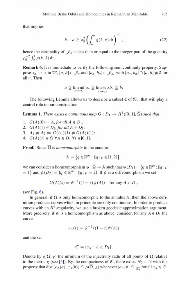
Definition 15. Let D ⊂ C, let h : [0, 1] × D → M be an admissible homotopy,γ ∈ D , and τ ∈ [0, 1]. We say that an interval [aτ , bτ ] ∈ Jh(τ,γ ) is h-genuine iffor all 0 � τ ′ � τ there exists [aτ ′ , bτ ′ ] ∈ Jh(τ ′,γ ) such that [aτ , bτ ] ⊂ [aτ ′ , bτ ′ ](see Fig. 8).

Now denote by

Jh(τ,γ ) = {[a1(τ, γ ), b1(τ, γ )], . . . , [am(τ, γ ), bm(τ, γ )]},(m =m(τ, γ )) the set of intervals in Jh(τ,γ ) (with bi <ai+1), which are h-genuine.Note that Jh(τ,γ ) is not empty and finite.

Definition 16. We call [a1(τ, γ ), b1(τ, γ )] the first h-genuine interval for (τ, γ ).

The following semi-continuity property of the first h-genuine interval holds.

Proposition 7. Let γn → γ in D , closed subset of C , and τn → τ . Then

a1(τ, γ ) � lim infn→+∞ a1(τn, γn) � lim sup

n→+∞b1(τn, γn) � b1(τ, γ ).


This portion correspondsto a non genuine h-interval

Fig. 8. The dotted curves in the figure represent part of the “evolution” of the curve γ bythe homotopy h. A portion of h(τ, γ ) corresponds to a crossing interval of h(τ, γ ) which isnot h-genuine. It arises from a non-crossing interval of γ

Proof. Set xn = h(τn, γn) and x = h(τ, γ ).Part 1

Suppose by contradiction that there exist γnk and τnk such that

a1(τnk , γnk ) −→ a < a1(τ, γ ). (42)

Since [a1(τnk , γnk ), b1(τnk , γnk )]∈Jxnkand [a1(τ, γ ), b1(τ, γ )]∈Jx we deduce

that there exists [α, β] ∈ Jx such that

a ∈ [α, β], β < a1(τ, γ ), lim supn→+∞

b1(τn, γn) � β, (43)

(see also Remark 6). Then [α, β] is not h-genuine for (τ, γ ), since [a1(τ, γ ),

b1(τ, γ )] is the first h-genuine interval for (τ, γ ). Then, by (42), (43) and (1) ofDefinition 11, we see that if k is sufficiently large, [a1(τnk , γnk ), b1(τnk , γnk )] isnot h-genuine, in contradiction with its definition.Part 2

Now suppose by contradiction that there exists γnk and τnk such that

b1(τnk , γnk ) −→ b > b1(τ, γ ). (44)

Then there exists [α, β] ∈ Jx such that

b ∈ [α, β], α > b1(τ, γ ), lim infn→+∞ a1(τn, γn) � α, (45)

(see also Remark 6).Now, for any k sufficiently large, there exists [αnk , βnk ] ∈ Jxnk

such that

[

lim infk→+∞ αnk , lim sup

k→+∞βnk

]

⊂ [a1(τ, γ ), b1(τ, γ )]. (46)


If [αnk , βnk ] is not h-genuine for (τnk , γnk ) for any k sufficiently large, by (1) ofDefinition 11 we deduce that [a1(τ, γ ), b1(τ, γ )]is not h-genuine in contradictionwith its definition. If there are infinitely many k’s such that [αnk , βnk ] is h-genuinefor (τnk , γnk ), and we again obtain a contradiction, since, in this case, there areinfinitely many k’s such that [a1(τnk , γnk ), b1(τnk , γnk )] is not the first h-genuineinterval for (τnk , γnk ), because, by (45) and (46), a1(τnk , γnk ) > βnk for any ksufficiently large.

Now, in order to move far from topologically non-essential intervals (see Def-inition 10) we need the following further property:

if [a, b] ∈ Jh(τ,γ ) is the first h-genuine interval for (τ, γ ),

then for all [α, β] ⊂ [a, b] topologically non-essential it is

φ(h(τ, γ )(s)) � −σ1

2for all s ∈ [α, β], (47)

where σ1 is defined in Remark 12.We finally define the following class of admissible homotopies:

H = {(D, h) : D is closed, R-invariant subset of C and

h : [0, 1] × D → M satisfies (40)–(41) and (47)} . (48)

Remark 15. Obviously it is crucial to have H = ∅. Towards this goal, using thegradient flow of the map φ in φ−1([−δ0, δ0]), we can assume the existence of ahomeomorphism ψ : � → A of class C1 on φ−1([−δ0, 0]) and such that ‖ψ‖E isconstant on any φ−1(δ) for any δ ∈ [0, δ0]. Then the map G of Lemma 1 is suchthat G(A) does not have topological non-essential intervals for any A ∈ D1, anddenoting by h0 the constant identity homotopy we have (C, h0) ∈ H .

In order to introduce the functional for our minimax argument, we set for any(D, h) ∈ H ,

F (D, h) = sup

{b − a

2

∫ b

ag(x, x) ds :

x = h(1, ξ), ξ ∈ D, [a, b] = [a1(1, ξ), b1(1, ξ)]}

, (49)

where [a1(1, ξ), b1(1, ξ)] is the first h-genuine interval for (1, ξ).

Remark 16. It is interesting to point out that the integral (b−a)2

∫ ba g(y, y) dt coin-

cides with 12

∫ 10 g(ya,b, ya,b) dt , where ya,b is the affine reparameterization of y on

the interval [0, 1].Remark 17. If ρ0 = inf{dist(x1, x2) : x1 ∈ D1, x2 ∈ D2} (where dist denotes thedistance induced by the Riemann structure g), it is

F (D, h) � 12ρ

20 , ∀(D, h) ∈ H . (50)

Moreover, by the definition of H we have

F (D, h) <M0

2, ∀(D, h) ∈ H . (51)


Given continuous maps h1 : [0, 1] × F1 → M and h2 : [0, 1] × F2 → Msuch that h1(1, F1) ⊂ F2, then we define the concatenation of h1 and h2 as thecontinuous map h2 � h1 : [0, 1] × F1 → � given by

h2 � h1(t, x) ={

h1(2t, x), if t ∈ [0, 12 ],

h2(2t − 1, h1(1, x)), if t ∈ [ 12 , 1]. (52)

7. Deformation Lemmas

To obtain the first deformation Lemma we first use a pseudo-gradient vectorfields technique to move away from curves with topological non-essential intervals.Then we use flows moving outside � when we are far from variationally criticalportions. Reparameterization flows are used when we are near irregular variation-ally critical portions of the second type. In this way we can build a homotopy alongwhich F takes smaller values when it assumes values far from topological criticallevels. Indeed, by the same proof in [10] we obtain

Proposition 8. (First Deformation Lemma) Let c ∈]0,M0[ be a geometrically reg-ular value (see Definition 4). Then it is a topologically regular value of F , that is,there exists ε = ε(c) > 0 having the following property: for all (D, h) ∈ H with

F (D, h) � c + ε

there exists a continuous map η ∈ C0 ([0, 1] × h(1,D),M) such that (D, η �h) ∈H and

F (D, η � h) � c − ε.

Now, in order to obtain the analogue of the classical second DeformationLemma, for any (D, h) and for any r∗ ∈ ]0, r ] let us consider the set:

Ur∗(D, h) = {

x = h(1, ξ) : ξ ∈ D

and there exists a crossing OGC ω : [a1(1, ξ), b1(1, ξ)]→� from D1 to D2 s.t.

‖x − ω‖a1(1,ξ),b1(1,ξ) � r∗}

, (53)

where [a1(1, ξ), b1(1, ξ)] is the the first h-genuine interval for (1, ξ).Assume now that the number of OGCs from D1 to D2 is finite. Then there exists

r > 0 such that the following two facts hold true:

for all r∗ ∈ ]0, r ] , for all x = h(1, ξ) ∈ Ur∗(D, h),

there exists at most one crossing OGC γ satisfying (53), (54)

and

the set C ≡ {A ∈ D1 : ‖A − ω(0)‖E < r

for some ω crossing OGC from D1 to D2} is contractible in D1, (55)

where ‖ · ‖E denotes the Euclidean norm.


Now define

C0 ≡ {

A ∈ M : |φ(A)| � δ0 and π(A) ∈ C}

(56)

where π denotes the projection onto ∂� along orthogonal geodesics.For any ρ > 0 and x ∈ M set B(x, ρ) = {y ∈ M : ‖x − y‖0,1 < ρ}. We have

the following crucial result:

Lemma 7. There exists r∗ ∈]0, r ] and ρ∗ > 0 having the following property:

∀x1, x2 ∈ Ur∗(D, h), xi = h(1, ξi ), i = 1, 2, and

∀z = h(1, ζ ) ∈ B(x1, ρ∗) ∩ B(x2, ρ∗) ∩ Ur∗(D, h), it is

z(s) ∈ C0 ∀s ∈ [min{a1(1, ξ1), a1(1, ξ2)},max{a1(1, ξ1), a1(1, ξ2)}],

where [a1(1, ξi ), b1(1, ξi )] is the first h-genuine interval for (1, ξi ), for any i = 1, 2.

Proof. Assume by contradiction the existence of rn → 0+, ρn → 0+, x1n , x2

n ∈Urn (D, h), xi

n = h(1, ξ in), i = 1, 2, zn = h(1, ζn) ∈ B(x1

n , ρn) ∩ B(x2n , ρn) ∩

Urn (D, h) and

sn ∈ [min{a1(1, ξ1n ), a1(1, ξ

2n )},max{a1(1, ξ

1n ), a1(1, ξ

2n )}] (57)

such that

zn(sn) ∈ C0, ∀ n.

Since B(x1n , ρn)∩ B(x2

n , ρn) = ∅ for any n, and D is compact, unless we wereto consider a subsequence, we have the existence of x = h(1, ξ) ∈ D such thatx1

n → x , x2n → x . Then zn → x , while, always up to considering a subsequence,

a1(1, ξ in) converges for any i = 1, 2.

By Proposition 7, we deduce that

[

lim infn→+∞ a1(1, ξ

in), lim sup

n→+∞b1(1, ξ

in)

]

⊂ [a1(1, ξ), b1(1, ξ)] ∀i = 1, 2.

Then, if [α, β] ⊂ [a1(1, ξ), b1(1, ξ)] is the interval such that x|[α,β] is a crossingOGC, we have

a1(1, ξin) → α ∀i = 1, 2.

Then by (57) we deduce that sn → α and therefore (since zn → x inH1,2([0, 1],Rm) we deduce also that zn(sn) → x(α) ∈ ∂� in contradiction withzn(sn) ∈ C0 for any n.

From now on, we fix r∗ as in Lemma 7. The same proof of the First DeformationLemma (cf. [10]) also allows us to obtain


Proposition 9. (Second Deformation Lemma) Let c be a geometrically criticalvalue. Then, there exists ε∗ = ε∗(c) > 0 such that, for all (D, h) ∈ H with

F (D, h) ⊂ ]−∞, c + ε∗],

there exists a continuous map η ∈ C0 ([0, 1] × h(1,D),M) such that η � h ∈ Hand:

F(

D \ h(1, ·)−1(Ur∗(D, h)), η � h)

⊂ ]−∞, c − ε∗].

The key to obtaining multiplicity results is the following Proposition.

Proposition 10. Assume that there are only a finite number of OGCs from D1 toD2. Then, for all h such that (D, h) ∈ H , there exists an open subset A of Cincluding the set h(1, ·)−1(Ur∗(D, h)), which is contractible in C.

For the proof we shall need the following:

Lemma 8. There exists a continuous map α : Ur∗(D, h) →]0, 1[ such that z(α(z))∈ C0 for any x ∈ Ur∗(D, h).

Proof. Take r∗ and ρ∗ as in Lemma 7. For any x ∈ Ur∗(D, h) consider B(x, ρ∗)∩Ur∗(D, h) ≡ B(x). Since Ur∗(D, h) is compact we can consider a finite open cov-ering of it, {B(xi )}i=1,...,k, xi ∈ Ur∗(D, h). If {βi }i=1,...,k is a continuous partitionof the unity subordinated to the above covering, we define

α(z) =k∑

i=1

βi (z)a1(1, ξi ),

where ξi is such that xi = h(1, ξi ) ∈ Ur∗(D, h) and a1(1, ξi ) is the first h-genuineinterval for (1, ξi ). Now, for any z ∈ Ur∗(D, h) we have

min{a1(1, ξ j ) : B(x j ) � z}k∑

i=1

βi (z) � α(z)

� max{a1(1, ξ j ) : B(x j ) � z}k∑

i=1

βi (z).

Since∑k

i=1 βi (z) = 1, by Lemma 7 we deduce that z(α(z)) ∈ C0 for any z ∈Ur∗(D, h).

Proof. (Proof of Proposition 10) Consider the homotopy h1 defined on [0, 1] ×{y(0) : y ∈ D}, induced by the homotopy h, and the homotopy h2 obtained bysending x(0) to x(α(x)) (where α is the continuous map obtained in Lemma 8)along the curve x , for any x ∈ Ur∗(D, h). Let P : ∂� → D1 be a continuousretraction extending the map π used in (56), whose existence is assured by thefact that ∂� is homeomorphic to an annulus. The homotopy P ◦ (h2 � h1) sends

{y(0) : y ∈ h(1, ·)−1(

Ur∗(D, h))

} in C , from which we deduce the contractibility

in C of h(1, ·)−1(

Ur∗(D, h))

. Since C is an ANR (see [19]) we have the thesis.


8. Proof of Theorems 1 and 4

We are now in the position of finalizing the plan outlined in Subsection 1.3.According to Definition 4 and Proposition 2, the proof of Theorems 1 and 4 willconsist in showing the corresponding multiplicity results for geometrically criticalvalues of the functional F . In our case, the geometrically critical values for F willbe the values of the lengths of the crossing OGCs.

Let us prove Theorem 1. For i = 1, 2, we set:

�i = {

D ⊂ C : D is closed and catC(D) � i}

, (58)

(see Subsection 1.3), and:

ci = infD∈�i

(h,D)∈H

F (h,D). (59)

We make the following observations:

1. ci � ρ20

2 , see (50),2. taking h = Id we have (h,C) ∈ H , so one immediately obtains (see (24)) the

following estimate:

ci � F (h,D) = supx∈C

1

2

∫ 1

0g(x, x) dt � 1

2M0.

3. �1 ⊃ �2, and therefore c1 � c2;4. each ci is a geometrically critical value of F . If by contradiction it were not,

let ε = ε(ci ) and η be given as in the thesis of the First Deformation Lemma(Proposition 8), let D ∈ �i and h be such that (h,D) ∈ H and

F (h,D) � ci + ε.

Since (η � h,D) ∈ H , it would be:

F (η � h,D) � ci − ε,

which is in contradiction with the definition of ci .5. c1 < c2. That is, assume by absurdity that c1 = c2 = c, let ε∗ > 0 be as in the

thesis of the Second Deformation Lemma (Proposition 9), and choose D ∈ �2such that (h,D) ∈ H with

F (h,D) � c + ε∗.

Let A be the open contractible subset of C containing h(1, ·)−1(

Ur∗(D, h))

given by Proposition 10. Consider D = D \ A ∈ �1. Now

F (η � h, D) � c − ε∗ = c1 − ε∗,

where η is as in the thesis of the Second Deformation Lemma. Since (η � h, D)belongs to the class H , we obtain a contradiction with the definition of c1.


This concludes the proof of Theorem 1. As to the proof of Theorem 4, it followsfrom a slight modification of the above proof, outlined briefly as follows. By sym-metry assumption there exists a Z2-action onMdescribed by an isometry I such thatI 2 = id. Right composition with I gives an isometry J (x) = I ◦ x on M such thatJ 2 = id. Choose a homeomorphism h : C → S

m−1, and let � : Sm−1 → RPm−1

be the projection onto the projective space RPm−1; recall that the Ljusternik–Sch-nirelman category of RPm−1 equals m. Replace the definition of the sets �i aboveby considering the sets

�i = {D ⊂ C : D is closed, J (D) = D , and

catRPm−1 (� (h(D))) � i}

, i = 1, . . . ,m. (60)

and:

ci = infD∈�i

(h,D)∈H

F (h,D). (61)

The key issue here is that the class of admissible homotopies can be chosen to beZ2-equivariant, that is, such that J ◦ h(τ, ·) = h(τ, ·) ◦ J , where τ ∈ [0, 1]. Usingthis fact, one proves that each ci is a geometrically critical value of F using theFirst Deformation Lemma, and that the values of the ci ’s are all distinct, using theSecond Deformation Lemma.

References

1. Ambrosetti, A., Coti Zelati, V.: Multiple homoclinic orbits for a class of conservativesystems. Rend. Sem. Mat. Univ. Padova 89, 177–194 (1993)

2. Benci, V., Fortunato, D., Giannoni, F.: Geodesics on static Lorentz manifolds withconvex boundary. In: Proceedings on Variational Methods in Hamiltonian Systems andElliptic Equations. Pitman Research Notes 243, 21–41 (1990)

3. Bos, W.: Kritische Sehenen auf Riemannischen Elementarraumstücken. Math. Ann.151, 431–451 (1963)

4. Coti Zelati, V., Rabinowitz, P.H.: Homoclinic orbits for second order Hamiltoniansystems possessing superquadratic potentials. J. Am. Math. Soc. 4, 693–727 (1991)

5. do Carmo, M.P.: Riemannian Geometry. Birkhäuser, Boston, 19926. Giambò, R., Giannoni, F.: Minimal geodesics on manifolds with discontinuous

metrics. J. Lond. Math. Soc. 67, 527 (2003)7. Giambò, R., Giannoni, F., Piccione, P.: Orthogonal geodesic chords, brake orbits and

homoclinic orbits in Riemannian manifolds. Adv. Differ. Equ. 10, 931–960 (2005)8. Giambò, R., Giannoni, F., Piccione, P.: On the multiplicity of brake orbits and homo-

clinics in Riemannian manifolds. Rend. Mat. Acc. Lincei, s. 9, 16, 73–85 (2005)9. Giambò, R., Giannoni, F., Piccione, P.: On the multiplicity of orthogonal geode-

sics in Riemannian manifold with concave boundary. Applications to brake orbits andhomoclinics. Adv. Nonlinear Stud. 9(4), 763–782 (2009)

10. Giambò, R., Giannoni, F., Piccione, P.: Existence of orthogonal geodesic chords onRiemannian manifolds with concave boundary and homeomorphic to the N -dimensionaldisk. Nonlinear Anal. Ser. A: Theory Methods Appl. 73, 290–337 (2010)

11. Giannoni, F., Majer, P.: On the effect of the domain on the number of orthogonalgeodesic chords. Differ. Geom. Appl. 7, 341–364 (1997)

12. Giannoni, F., Masiello, A.: On the existence of geodesics on stationary Lorentz man-ifolds with convex boundary. J. Funct. Anal. 101, 340–369 (1991)


13. Giannoni, F., Rabinowitz, P.H.: On the multiplicity of homoclinic orbits on Riemann-ian manifolds for a class of second order Hamiltonian systems. Nonlinear Differ. Equ.Appl. 1, 1–46 (1994)

14. Gluck, H., Ziller, W.: Existence of periodic motions of conservative systems. In:Seminar on Minimal Surfaces (Bombieri, E. Ed.). Princeton University Press, 65–98,1983

15. Long, Y., Zhu, C.: Closed characteristics on compact convex hypersurfaces in R2n .

Ann. Math. (2) 155(2), 317–368 (2002)16. Lusternik, L., Schnirelman, L.: Methodes Topologiques dans les Problemes Varia-

tionelles. Hermann, 193417. Mahwin, J., Willem, M.: Critical Point Theory and Hamiltonian Systems. Springer-

Verlag, New York-Berlin, 198818. Peturel, E.: Multiple homoclinic orbits for a class of Hamiltonian systems. Calc. Var.

PDE 12, 117–143 (2001)19. Palais, R.: Homotopy theory on infinite dimensional manifolds. Topology 5, 1–16

(1966)20. Rabinowitz, P.H.: Periodic and heteroclinic orbits for a periodic Hamiltonian system.

Ann. Inst. H. Poincaré, Analyse Non Lineaire 6, 331–346 (1989)21. Seré, E.: Existence of infinitely many homoclinic orbits in Hamiltonian systems. Math.

Z. 209, 27–42 (1992)22. Seré, E.: Looking for the Bernoulli shift. Ann. Inst. H. Poincaré, Analyse Non Lineaire

10, 561–590 (1993)23. Spanier, H.: Algebraic Topology. McGraw-Hill, New York, 196624. Struwe, M.: Variational Methods. Applications to Nonlinear Partial Differential Equa-

tions and Hamiltonian Systems, 3rd edn. Springer-Verlag, Berlin, 200025. Tanaka, K.: A note on the existence of multiple homoclinic orbits for a perturbed radial

potential. Nonlinear Differ. Equ. Appl. 1, 149–162 (1994)

Scuola di Scienze e Tecnologie, Sezione Matematica,Università di Camerino,

Via Madonna delle Carceri,62032 Camerino,

MC, Italy.e-mail: [email protected]: [email protected]

and

Departamento de Matemática,Universidade de São Paulo,

Rua do Matão, 1010,São Paulo,

SP 05508-090,Brazil.

e-mail: [email protected]

(Received May 4, 2010 / Accepted August 20, 2010)Published online September 14, 2010 – © Springer-Verlag (2010)

Documents

Multiple Brake Orbits and Homoclinics in Riemannian Manifolds