Multiplier decomposition within Regional SAMs: the case of Andalusia

Multiplier Decomposition within Regional SAMs: the case of Andalusia*

M. Carmen Lima Universidad Pablo de Olavide de Sevilla

M. Alejandro Cardenete Universidad Pablo de Olavide de Sevilla & centrA

ABSTRACT

In this work we present a methodology of multipliers decomposition (including an employment

multiplier), for a regional economy as Andalusia using Social Accounting Matrices (SAM). These

matrices are able to enlarge the information provided by the input-output analysis, because they

complete the interindustrial flows of an economy with the behaviour of productive factors,

consumers, public sector and foreign sector. This database allows us to capture conclusions about

intersectoral dependences in a region in a double sense: firstly, from a partial perspective based on

the results derived for every year, and secondly from an structural point of view along the decade

of the nineties.

Keywords: social accounting matrix, regional accounting, structural analysis. JEL classification: C67, D57, R15. correspondence to: M. Carmen Lima Díaz

Department of Economy and Business Universidad Pablo de Olavide at Seville Ctra. Utrera, km.1 41013-Sevilla, Spain Phone number: +(34) 954349353

e-mail: [email protected]

* The first two authors wish to thank the support from XT 2002-00037 and centrA (Fundación Centro de Estudios Andaluces). The second author also thanks to SEC 2003-05112/ECO and FEDER.

mailto:[email protected]

1. Introduction

Social accounting matrices (SAM) are databases comprising economic transactions and

information about the economic agents such as the producers, the consumers, the

government and the foreign sector; as well as the productive factors. They complete the

information provided by the input-output analysis (IOA thereafter), with the regional or

national accounting and the surveys of family constraints, among other databases.

The interest on SAMs is based on the fact that not only do they study the production

relationships among the economic sectors, but also the transactions that take place among

the different institutions of an economic system in terms of revenues or consumption.

Besides their statistical content, the SAMs have became an useful instrument for

evaluation of interventions from the political economy in national or regional economies.

If a SAM is available for more than one year, it is feasible to carry out a complete analysis

of the productive structure and a perspective of the changes that have occurred. Several

methodologies are able to outline such analysis in a particular economy and we develop

one of them in this paper, the so called multiplier decomposition. In the next section, we

apply the classical multiplier decomposition methodology to derive the own, open and

circular effects. In section three we proceed to calculation of an employment multiplier in

order to get some valuable information in terms of elasticity between economic activity

and capacity of employment creation. In section four, we come up with an empirical

application of this methodology on the SAMs for Andalusia in the years 1990 and 1995

which have been elaborated in previous works1. We will also use a first estimate for the

SAM for Andalusia 19992. This exercise will point out the multipliers decomposition for

this regional economy, the type of interrelationships and the nature of linkages inside it. In

section five we outline the main results and conclusions.

2. The classical multiplier decomposition applied to Social Accounting Matrices.

In this paper we work with multisectoral linear models, in which we assume the

exogeneity of the prices. We consider as endogenous those accounts that are part of the

2

economic interrelations determined outside of the economic system (production factors,

productive sectors and private sector); while the exogenous ones are tools for the political

economy (as the public sector, foreign sector and capital)3.

The multipliers decomposition methodology was initially proposed by Stone (1978) and

Pyatt and Round (1979). Later on, Defourney and Thorbecke (1984) and again Pyatt and

Round (1985) have been working on it. We also have Spanish references as those by Polo,

Roland-Holst and Sancho (1991), among others. It is also interesting to highlight the works

from the regional point of view developed by Cardenete and Sancho (2003) for Andalusia,

de Miguel, Manresa and Ramajo (1998) for Extremadura or Llop and Manresa (2003) for

Catalonia.

The formulation of these linear models of general equilibrium is the following:

Let be: ny

( nn AIy −= )-1 ⋅ x = Ma ⋅ x (1)

where is the column vector of total rents of the endogenous accounts, I is an identity

matrix of order n x n, An is the average tendency matrix of expenditure between the

different endogenous accounts and x is the vector that collects the flows of rent that the

endogenous accounts receive from the exogenous ones.

ny

A generic element of An as aij is interpreted as the expense carried out in i per each unit of

expense of the sector j. Ma is the so called Accounting Multipliers Matrix and an element

maij indicates the effect that an exogenous unit of rent on an endogenous account j,

generates on the rent of the endogenous account i. In other words, the interpretation would

be how many monetary units of rent are generated in sector i because of the circular flow

of rent when sector j receives a unitary shock. If we sum up these values of Ma by

columns, we get the total effect of an exogenous shock received by one account on the rest

of the economic activity. This way, the account with the greatest multiplier value points

out one sector with an important influence on the rest of the economy when it is involved

in an economic development policy.

3

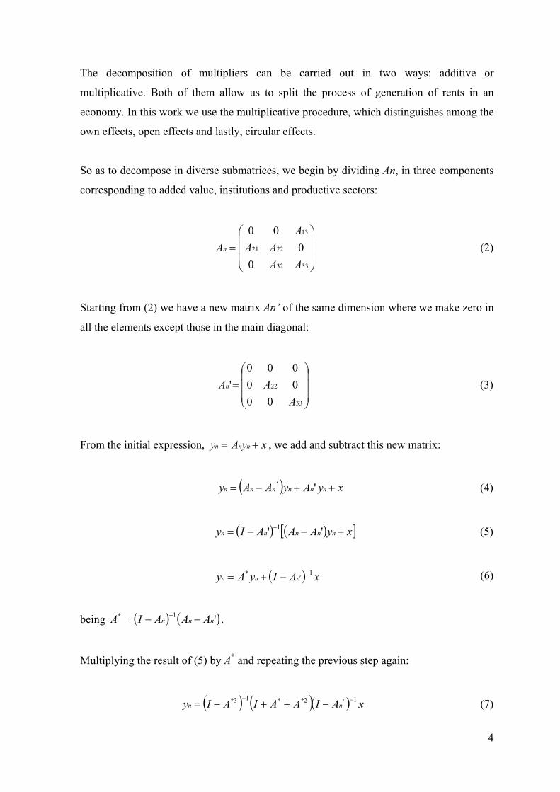
The decomposition of multipliers can be carried out in two ways: additive or

multiplicative. Both of them allow us to split the process of generation of rents in an

economy. In this work we use the multiplicative procedure, which distinguishes among the

own effects, open effects and lastly, circular effects.

So as to decompose in diverse submatrices, we begin by dividing An, in three components

corresponding to added value, institutions and productive sectors:

=

3332

2221

13

00

00

AAAA

AAn (2)

Starting from (2) we have a new matrix An’ of the same dimension where we make zero in

all the elements except those in the main diagonal:

(3)

=

33

22

0000000

'A

AAn

From the initial expression, , we add and subtract this new matrix: xyAy nnn +=

( ) xyAyAAy nnnnnn ++−= '' (4)

( ) ( )[ xyAAAIy nnnnn +−−= − '' 1 ]

)

(5)

( ) xAIyAy nnn1* −

′−+= (6)

being . ( ) ( '1*nnn AAAIA −−= −

Multiplying the result of (5) by A* and repeating the previous step again:

( ) ( )( ) xAIAAIAIy nn12**13* ' −−

−++−= (7)

4

Finally we get:

(8) xMaMaMayn 123=

We have decomposed the matrix of countable multipliers in other three matrices by means

of a multiplicative expression following Pyatt and Round (1979). The first matrix, is called

matrix of circular effects and reflects the effect that an exogenous injection of rent

generates on the very account due to the circular flow of the rent. By further calculations,

we reach the following diagonal expression, since it does not pick up any type of crossed

effect:

( ) ( )[ ]( ) ( )[ ]

( ) ( )[ ]

−−−

−−−

−−−

=−−−

−−

−−

−

−

11321

12232

133

132331321

122

1212232

13313

3

00

00

001

1

AAAIAAII

AAIAAAII

AAIAAIAI

Ma

(9)

The second matrix, is known as the matrix of open or crossed effects, and the elements of

its main diagonal are identity submatrices. It shows the effects on the rest of accounts of a

shock received by one particular account. Its expression is as follows:

( )( ) ( )

( ) ( ) ( )

−−−−−

−=

−−−

−−

−

IAAIAAIAAIAAAIIAAI

AAAIAIMa

321

33211

22321

33

13211

22211

22

13323313

2

1

(10)

Finally, we have the matrix of own or internal effects, also known as matrix of transfers

because the first element of the main diagonal is an identity submatrix (there are no

transfers among the productive factors), the second shows the transactions among

institutions and the later includes the interindustrial transactions, and is in fact the inverse

of Leontief. The expression is as follows:

5

(11) ( )( )

−−=

−

−

133

1221

000000

AIAI

IMa

To interpret the multiplicative decomposition in terms of relative importance of each

element on the total effect, we can express the equation (8) by means of an additive

transformation:

(12) ( ) ( ) ( ) 123121 MaMaIMaMaIMaIMaIMa −+−+−+=

3. The employment multipliers

In the previous expression, the identity matrix allows to discount the initial injection of

rent of each of the effects, so that we work with a net multiplicative decomposition. It is

possible to calculate one more multiplier to extract the accounts that generate more

employment when receiving a unitary exogenous injection of rent. The employment

multipliers are the result, in the first place, of a new diagonal matrix that we call E. This

matrix includes the quotients between the volume of employment and the total resources

for each productive sector. In the second place, we multiply this matrix with the part of Ma

that incorporates the rows and columns corresponding to the productive sectors (in our

case the order of this matrix is 10x13). When increasing the rent of an endogenous account,

we will obtain the effects of this change in the corresponding column of the partition of Ma

and, by means of the diagonal matrix E, we convert this impact into number of jobs. This

way the expression of the employment multiplier, Me, is the following:

(13) MaEMe *=

An element meij, is the increment experienced in the volume of employment of the sector i

when the sector j receives a unitary exogenous injection4. If we analyse the sum of

columns, we have the effect on the employment at a global level, which entails the

reception of an exogenous monetary unit on a particular sector. As far as rows is

concerned, they show the increment that the activity sector in question experiences in its

6

employment if the rest of sectors receive the exogenous monetary unit. As we are dealing

with very small figures in absolute terms, we proceed to the normalization of the

multipliers based on the average values by row and column and total average value. We get

the new results by following these steps:

- We calculate the columns and row average values.

- We derive the total average value by means of the sum of all the values of Me divided by

the number of elements of Me.

- We divide the average values by rows and columns by the total average value. If the

result is greater than 1, the normalized figure indicates an employment multiplier over the

average.

By this process we can carry out comparisons that can be easily interpreted. Accordingly,

they can be used as a reference to contrast if a value is greater than what we consider an

average reaction or not. Thereby, we get a classification of sectors that are able to

transform its activity increments into new employment.

4. Empirical application to Andalusian economy

By applying the previous theoretical analysis on the SAM of Andalusia, we have obtained

four types of multipliers: those that measure the own, open, circular effects, and finally, the

employment multipliers. If we had carried out a decomposition of multipliers on the

inverse of Leontief’s theory instead of on the SAM, we would have found the limitation

that the first one has no capacity to measure the feedback effects or interdependences

generated by an exogenous shock on the final demand of a particular sector. That is to say,

the multipliers obtained working with SAMs incorporate all the flows that take place

between the institutions and the productive sectors (the induced effects if we carry out an

additive multipliers decomposition or the circular effects if we follow the terminology of

the multiplicative one). Therefore, we can affirm that the difference between the

multipliers calculated according to the SAM and the input-output ones, is in fact the value

of this third multiplier that captures the feed-back again from the institutions toward the

7

activity sectors, once the initial impulse has been transmitted from the productive sectors to

the institutions.

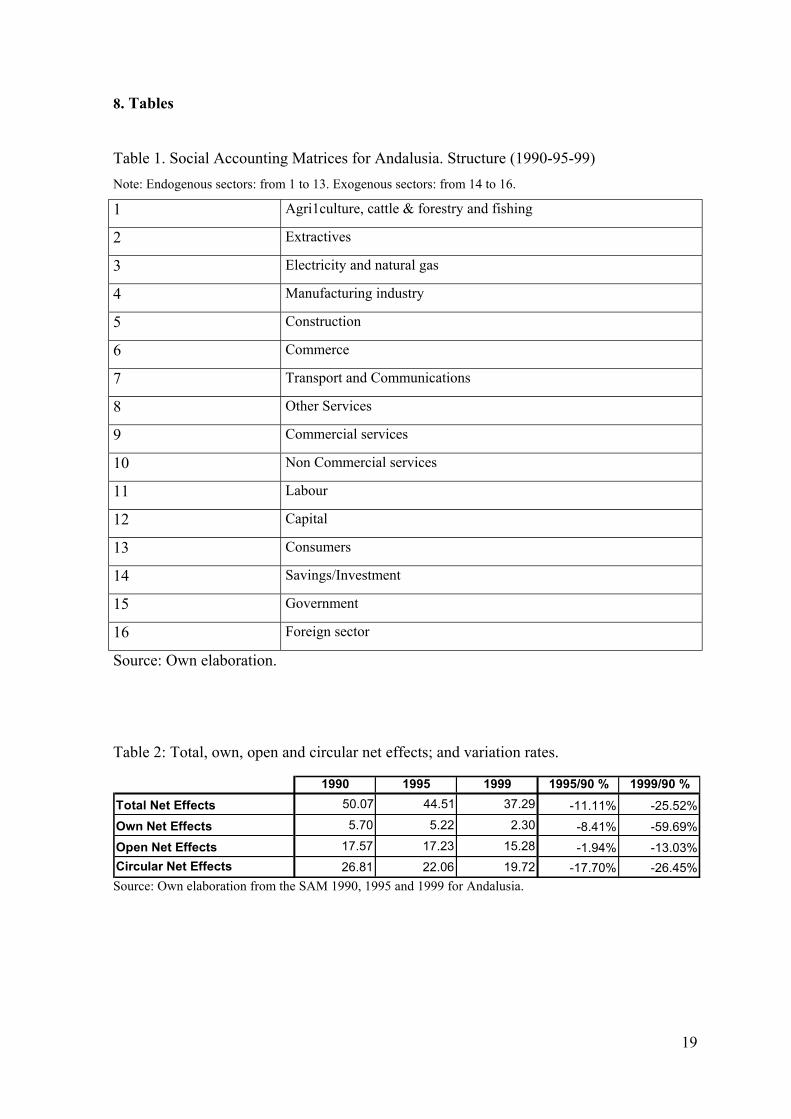
To start with, we outline the structure of the SAM we are using. Such SAMs for Andalusia

belong to the years 1990, 1995 and an approach to 1999 by means of an updating

technique called Cross Entropy Method (CEM) on the SAM for 1995. In our endogenous

accounts we find the two productive factors (capital and labour), the private sector

represented by the consumers and finally ten activity sectors. Our exogenous accounts,

following the most common approaches in the literature are three: public sector, savings

and investment, and foreign sector. Our three databases have been added to 16 accounts as

it is shown in the following table:

(Table 1, Page 19)

With relation to the information on the following tables, we present the value of the

multipliers firstly by rows and secondly by columns, although logically, the partial or total

added value of the multipliers for every year is the same regardless of the presentation we

choose.

The data in the following tables are derived from carrying out a transformation on the

multiplicative decomposition. This transformation consists in expressing in an additive

way for an easier interpretation and comparison. The data are presented in absolute and

percentage terms, in order to quantify the relative importance of each of the mechanisms of

transmission of the shocks experienced by the regional economy.

All the following tables are structured in the same way: we display the net total effects of

the unitary shock in the first column. In the second, the own net effects are picked up. In

the third column the open effects are shown so as to measure the impact on the whole

economy of a rent injection received by one account. Finally, we have the circular effects

to catch up the reaction of the exogenous accounts as a result of the circular flow of the

rent.

8

The results of the multipliers decomposition for the Andalusian economy throughout the

nineties, show that the effects that register a bigger weight in relation to the others, are the

circular ones, followed by the open effects and last by the own effects. The role played by

the circular effects reaffirms the importance of using SAMs instead of IO tables. There is

a single exception to the leadership of the circular effects, namely, labour factor and

consumers; in this case, the order of importance between circular and open effects is

inverted. This circumstance is similar to the case of the capital factor, although slightly

softer.

From a global perspective of the decade, the multipliers measured at added level reach the

highest values in 1990, with a descending tendency up to 1999 (this one is next to 60% in

some of the cases, see for example Table 2, where the variation rates have been

calculated).

(Table 2, Page 19)

We can observe how a widespread decrease has taken place since 1990. The highest value

for 1995 is 17.70% of decrement of the circular net effects. This descent is even stressed in

1999, when there is an outstanding fall of the own net effects (it almost reaches 60%),

followed by the circular ones with more than 25%. Finally, the open net effects are not so

affected (13.03%). In general the data show a reduction in terms of total effects so that the

variation rate is doubled from one period to the other.

If we analyse Table 3 with the aggregate multipliers for 1990, it shows the general

behaviour where the circular effects have a high weight that surpasses 40% of the total net

effects at the worst, and at best they represent more than 60% (“Extractives” (2) and

“Trade and Repair” (9) respectively). The next ones are the open net effects that vary

around 30% with the exceptions of the productive factors whose data are considerably

bigger, and the “Extractives” (2) whose value is smaller than average. Finally, we have the

own net effects with an the oscillation band of 5.14% for “Trade and Repair" (9) in the

lower bound and again the “Extractives” (2) ones in the upper with 35.05%.

9

It is interesting to highlight out the homogeneous behaviour of the sectors corresponding to

“Agriculture, Cattle & Forestry and Fishing" (1), "Construction" (5) and all the services in

general (from accounts (5) to (10)) with the mentioned exceptions. Another example of

similar behaviour is that of the productive factors and the private sector (from account (11)

to (13)), while a third block corresponds to the industrial sectors (from (3) and (4)). Lastly,

we want to highlight an outlier value included in “Extractives” (2).

(Table 3, Page 20)

Table 4 presents the results of the multipliers decomposition are shown for 1990 by rows.

The biggest values are registered by productive factors together with the private sector. It

is also important the role played by the open effects for these three accounts, while the

own effects grow in the rest, which is an aspect that is compensated by a reduction in the

open effects.

(Table 4, Page 20)

Next we show the results corresponding to 1995, firstly, by columns in Table 5 and

secondly by rows in Table 6:

(Table 5, Page 21)

For 1995, the circular net effects continue at the top although they register a small fall with

respect to the previous year. In spite of this, in most of the accounts they explain more than

50% of the total effect, showing the important feedback of an exogenous shock. The open

effects also consolidate positions to the detriment of the own net effects that present a

stationary behaviour in the accounts (1), (3), and (4) and a reduction in the rest. In relation

to these last effects, again we verify that for the productive factors and the private sector,

their value is 0 as we had previously argued.

(Table 6, Page 21)

10

As far as rows is concerned, the circular effects are smaller, with some cases of reduction

of the multiplier like in "Construction" (5) where there is a fall of more than 50%. The

open net effects are also smaller than in columns while the own net effects grow in most of

the cases. We verify that these are zero in the same way as in the whole decade for the

accounts (11), (12) and (13).

In the third year of analysis, the circular net effects are again the greatest ones as it

happened in the other years. The open effects grow slightly with the exception of the

accounts of the productive factors and consumers. Similar behaviours are reflected in the

Tables 7 and 8.

(Table 7, Page 22)

(Table 8, Page 22)

So as to be able to compare the multipliers by means of a temporary analysis, we have

elaborated a group of figures where the different effects are taken into account:

(Figure 1, Page 23)

As we observe in Figure 1, the highest multipliers both in absolute terms and in

disaggregated level for each effect, are those of 1990. This shows a bigger activity of the

economy before a monetary injection comes from any of the exogenous accounts. In

Figure 3 we carry out a comparative analysis of each block of effects through a bars

diagram. In this graph we find a certain harmony in the accounts with bigger total effects

all through the decade. Those accounts are the “Commercial services”(9), “Non

Commercial services” (10) and “Capital"(12). Only for “Commerce"(6), the total effects of

1995 are able to go above those of 1990. Lastly, it is interesting to analyse the important

fall in the total effects for some sectors in 1999, for example “Manufacturing industry"(4)

or “Extractives” (2), which was a common behaviour in the rest of accounts with the

exception of "Labour" (11).

(Figure 2, Page 23)

11

The own net effects only take values for the accounts corresponding to the activity sectors,

showing a descending tendency with the exception of the “Construction"(5). This account

increases from 16.54% to 24.46%, and falls in the last year up to 11.25%.

(Figure 3, Page 24)

The open net effects register a very homogeneous behaviour during the whole decade,

growing steadily from 1990 to 1999. The productive factors and the private sector behave

different from the rest, with higher values for the whole period. The circular effects remain

stable between 40% and 60%, and the highest multipliers correspond to services and

specially to “Commercial services" (6).

(Figure 4, Page 24)

(Figure 5, Page 25)

Working on different endogeneity criteria is an interesting exercise to deepen in the

relative weight of the mentioned interdependences. Although this is not the object of the

present work, we can conclude that whenever we include one more endogenous sector in

the analysis, the immediate result is an increment in the value of the multipliers. This is

because more variables are part of the feedback flow.

We present now the employment multipliers for the Andalusian economy. The column

analysis let us see that the effect on employment of the reception of a monetary unit

coming from an exogenous account. Therefore, by means of the revision of the data given

by the sum of rows, we can test the increase experienced in the employment of each

activity sector after a positive shock on the final demand of the economy.

The present employment multipliers have been normalized by columns and rows. They are

very relevant because they can be compared in relation to the average of the sector and

with regard to the total average of productive sectors. As we already explained in the

previous section, it has been necessary to build a diagonal matrix for every year to obtain

12

the figure of employment in relation to the total output of the sector. If we apply the

coefficients of the SAM, the ten rows of the productive sectors and the thirteen

endogenous accounts for columns to the previous ratio, we get these new multipliers.

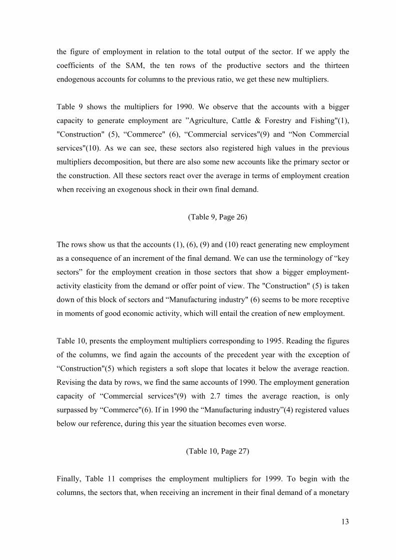
Table 9 shows the multipliers for 1990. We observe that the accounts with a bigger

capacity to generate employment are ”Agriculture, Cattle & Forestry and Fishing"(1),

"Construction" (5), “Commerce" (6), “Commercial services"(9) and “Non Commercial

services"(10). As we can see, these sectors also registered high values in the previous

multipliers decomposition, but there are also some new accounts like the primary sector or

the construction. All these sectors react over the average in terms of employment creation

when receiving an exogenous shock in their own final demand.

(Table 9, Page 26)

The rows show us that the accounts (1), (6), (9) and (10) react generating new employment

as a consequence of an increment of the final demand. We can use the terminology of “key

sectors” for the employment creation in those sectors that show a bigger employment-

activity elasticity from the demand or offer point of view. The "Construction" (5) is taken

down of this block of sectors and “Manufacturing industry" (6) seems to be more receptive

in moments of good economic activity, which will entail the creation of new employment.

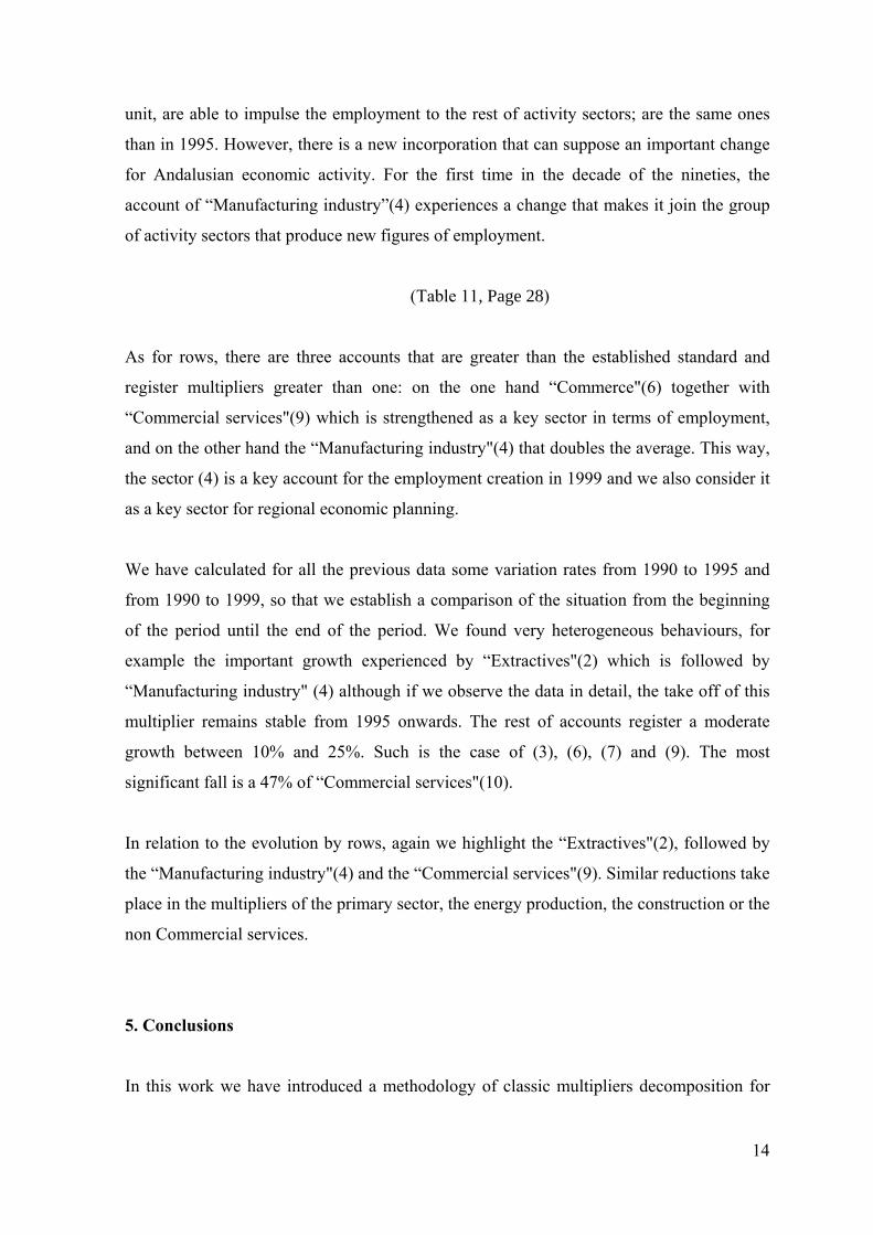
Table 10, presents the employment multipliers corresponding to 1995. Reading the figures

of the columns, we find again the accounts of the precedent year with the exception of

“Construction"(5) which registers a soft slope that locates it below the average reaction.

Revising the data by rows, we find the same accounts of 1990. The employment generation

capacity of “Commercial services"(9) with 2.7 times the average reaction, is only

surpassed by “Commerce"(6). If in 1990 the “Manufacturing industry”(4) registered values

below our reference, during this year the situation becomes even worse.

(Table 10, Page 27)

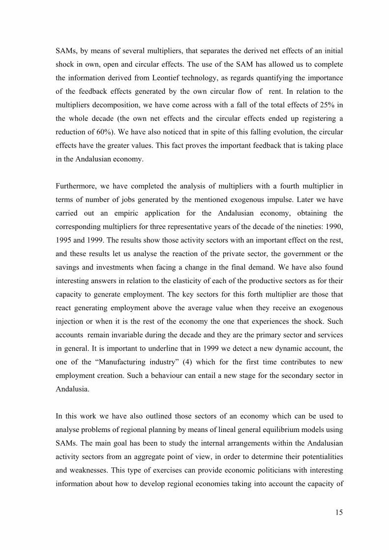
Finally, Table 11 comprises the employment multipliers for 1999. To begin with the

columns, the sectors that, when receiving an increment in their final demand of a monetary

13

unit, are able to impulse the employment to the rest of activity sectors; are the same ones

than in 1995. However, there is a new incorporation that can suppose an important change

for Andalusian economic activity. For the first time in the decade of the nineties, the

account of “Manufacturing industry”(4) experiences a change that makes it join the group

of activity sectors that produce new figures of employment.

(Table 11, Page 28)

As for rows, there are three accounts that are greater than the established standard and

register multipliers greater than one: on the one hand “Commerce"(6) together with

“Commercial services"(9) which is strengthened as a key sector in terms of employment,

and on the other hand the “Manufacturing industry"(4) that doubles the average. This way,

the sector (4) is a key account for the employment creation in 1999 and we also consider it

as a key sector for regional economic planning.

We have calculated for all the previous data some variation rates from 1990 to 1995 and

from 1990 to 1999, so that we establish a comparison of the situation from the beginning

of the period until the end of the period. We found very heterogeneous behaviours, for

example the important growth experienced by “Extractives"(2) which is followed by

“Manufacturing industry" (4) although if we observe the data in detail, the take off of this

multiplier remains stable from 1995 onwards. The rest of accounts register a moderate

growth between 10% and 25%. Such is the case of (3), (6), (7) and (9). The most

significant fall is a 47% of “Commercial services"(10).

In relation to the evolution by rows, again we highlight the “Extractives"(2), followed by

the “Manufacturing industry"(4) and the “Commercial services"(9). Similar reductions take

place in the multipliers of the primary sector, the energy production, the construction or the

non Commercial services.

5. Conclusions

In this work we have introduced a methodology of classic multipliers decomposition for

14

SAMs, by means of several multipliers, that separates the derived net effects of an initial

shock in own, open and circular effects. The use of the SAM has allowed us to complete

the information derived from Leontief technology, as regards quantifying the importance

of the feedback effects generated by the own circular flow of rent. In relation to the

multipliers decomposition, we have come across with a fall of the total effects of 25% in

the whole decade (the own net effects and the circular effects ended up registering a

reduction of 60%). We have also noticed that in spite of this falling evolution, the circular

effects have the greater values. This fact proves the important feedback that is taking place

in the Andalusian economy.

Furthermore, we have completed the analysis of multipliers with a fourth multiplier in

terms of number of jobs generated by the mentioned exogenous impulse. Later we have

carried out an empiric application for the Andalusian economy, obtaining the

corresponding multipliers for three representative years of the decade of the nineties: 1990,

1995 and 1999. The results show those activity sectors with an important effect on the rest,

and these results let us analyse the reaction of the private sector, the government or the

savings and investments when facing a change in the final demand. We have also found

interesting answers in relation to the elasticity of each of the productive sectors as for their

capacity to generate employment. The key sectors for this forth multiplier are those that

react generating employment above the average value when they receive an exogenous

injection or when it is the rest of the economy the one that experiences the shock. Such

accounts remain invariable during the decade and they are the primary sector and services

in general. It is important to underline that in 1999 we detect a new dynamic account, the

one of the “Manufacturing industry” (4) which for the first time contributes to new

employment creation. Such a behaviour can entail a new stage for the secondary sector in

Andalusia.

In this work we have also outlined those sectors of an economy which can be used to

analyse problems of regional planning by means of lineal general equilibrium models using

SAMs. The main goal has been to study the internal arrangements within the Andalusian

activity sectors from an aggregate point of view, in order to determine their potentialities

and weaknesses. This type of exercises can provide economic politicians with interesting

information about how to develop regional economies taking into account the capacity of

15

key sectors to produce economic activity. We also argue for the idea of space association

in order to obtain an integrated regional development and a greater effectiveness on the

efforts of regional policy.

6. Notes

1 See Cardenete, M.A. (1998), and Cardenete, M. A. and Moniche, L. (2001), respectively. 2 This first version has been calculated by the application of an updating technique called

CEM (Cross Entropy Method) on the SAM for Andalusia 1995, carried out by Cardenete,

M.A. and Sancho, F. (2002). Using this methodology, we can introduce known information

inside the cells of the estimated SAM (prior information), letting us to use it for structural

analysis because there are changes in the technical coefficients (see Robinson et al. (2001)) 3 Revising the literature, there are alternative classifications, for example the ones

proposed by Polo, C., Roland-Holst, D. and Sancho, F. (1991) that endogenizes the capital

account, or that of Llop, M. and Manresa, A. (2003) with an external sector

endogenezation. 4 Additional information about the employment multiplier and a comparison with other

type of multipliers, is provided in Arango (1979).

16

7. References

Arango, J. (1979): ”Multiplicadores derivados de un modelo input-output regional”,

Investigaciones Económicas, nº 8, pp. 5-26.

Bosch, J. et alia (1997): ”Evaluación del Impacto Económico de la Construcción de la Red de

Cable de Banda Ancha en Cataluña”, Institut D’Estudis Territorials, Barcelona.

Cardenete, M.A. (1998): “Una matriz de contabilidad social para la economía andaluza: 1990”,

Revista de Estudios Regionales, 52 pp. 137-153.

Cardenete, M.A. & Moniche, L. (2001): “El nuevo marco input-output y la SAM de Andalucía

para 1995 “, Cuadernos Ciencias Económicas y Empresariales nº 41, pp. 13-32.

Cardenete, M.A. & Sancho, F. (2002): “Sensitivity of simulation results to competing SAM

updated”, Working Paper 556.02, Departamento de Fundamentos del Análisis Económico (UAB),

Instituto de Análisis Económico, CSIC.

Cardenete, M.A. & Sancho, F. (2003): “Evaluación de multiplicadores contables en el marco de

una matriz de contabilidad social regional”, Investigaciones Regionales nº 2, pp. 121-139.

Curbelo Ranero, J.M. (1986): “Una introducción a las Matrices de Contabilidad Social y a su uso

en la Panificación del Desarrollo Regional”, Estudios Territoriales nº 7, pp. 147-155.

Defourney, J. & Thorbeke, E. (1984): “Structural Path Analysis and Multiplier Decomposition

within a Social Accounting Matrix framework”, The Economic Journal, nº 94, pp. 111-136.

De Miguel, F.J., Manresa, A, & Ramajo, J. (1999): “Matriz de Contabilidad Social y

multiplicadores contables: una aplicación para Extremadura”, Estadística Española, Vol. 40, nº

143, pp. 195-232.

Kehoe, T.J., Manresa, A., Polo, C. & Sancho, F. (1988): ” Una matriz de contabilidad social de la

economía española”, Estadística Española, Vol. 30, nº 117, pp. 5-33.

Llop, M. & Manresa, A. (2003): “Análisis de multiplicadores lineales en una economía abierta”,

Working Paper Serie de Economía E/2002/21, Fundación Centro de Estudios Andaluces (centrA).

17

Pyatt, G. & Round, J. (1985): Social Accounting Matrices: a basis for Planning, The World Bank,

Washington.

Polo, C. Roland-Holst, D.W. & Sancho, F. (1991): “Descomposición de multiplicadores en un

modelo multisectorial: Una aplicación al caso español”, Investigaciones Económicas, Vol. XV, nº

1.

Roland Holst, D.W. (1990): “Interindustry analysis with Social Accounting Methods”, Economic

Systems Research,Vol. 2, nº 2, pp. 125-145.

Stone, R. (1978): The Disagreggation of the Household Sector in the National Accounts, World

Bank Conference on Social Accounting Methods in Development Planning, Cambridge.

18

8. Tables

Table 1. Social Accounting Matrices for Andalusia. Structure (1990-95-99) Note: Endogenous sectors: from 1 to 13. Exogenous sectors: from 14 to 16.

1 Agri1culture, cattle & forestry and fishing

2 Extractives

3 Electricity and natural gas

4 Manufacturing industry

5 Construction

6 Commerce

7 Transport and Communications

8 Other Services

9 Commercial services

10 Non Commercial services

11 Labour

12 Capital

13 Consumers

14 Savings/Investment

15 Government

16 Foreign sector

Source: Own elaboration.

Table 2: Total, own, open and circular net effects; and variation rates.

1990 1995 1999 1995/90 % 1999/90 %Total Net Effects 50.07 44.51 37.29 -11.11% -25.52%Own Net Effects 5.70 5.22 2.30 -8.41% -59.69%Open Net Effects 17.57 17.23 15.28 -1.94% -13.03%Circular Net Effects 26.81 22.06 19.72 -17.70% -26.45%Source: Own elaboration from the SAM 1990, 1995 and 1999 for Andalusia.

19

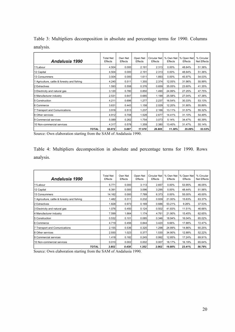
Table 3: Multipliers decomposition in absolute and percentage terms for 1990. Columns

Source: Own

analysis.

elaboration starting from the SAM of Andalusia 1990.

able 4: Multipliers decomposition in absolute and percentage terms for 1990. Rows

Andalusia 1990 Total Net Effects

Own Net Effects

Open Net Effects

Circular Net Effects

% Own Net Effects

% Open Net Effects

% Circular Net Effects

11Labour 4.504 0.000 2.191 2.313 0.00% 48.64% 51.36%

12 Capital 4.504 0.000 2.191 2.313 0.00% 48.64% 51.36%

13 Consummers 3.504 0.000 1.611 1.893 0.00% 45.97% 54.03%

1 Agriculture, cattle & forestry and fishing 4.240 0.511 1.355 2.374 12.05% 31.96% 55.99%

2 Extractives 1.593 0.558 0.376 0.659 35.05% 23.60% 41.35%

3 Electricity and natural gas 3.120 0.780 0.850 1.490 24.99% 27.25% 47.75%

4 Manufacturer industry 2.531 0.647 0.685 1.199 25.58% 27.04% 47.38%

5 Construction 4.211 0.696 1.277 2.237 16.54% 30.33% 53.13%

6 Commerce 3.631 0.443 1.158 2.029 12.20% 31.90% 55.89%

7 Transport and Comunications 3.916 0.513 1.237 2.166 13.11% 31.57% 55.32%

8 Other services 4.912 0.708 1.528 2.677 14.41% 31.10% 54.49%

9 Commercial services 5.089 0.262 1.754 3.073 5.14% 34.47% 60.39%

10 Non-commercial services 4.317 0.578 1.359 2.380 13.40% 31.47% 55.14%

TOTAL 50.072 5.697 17.570 26.805 11.38% 35.09% 53.53%

T

analysis.

Source: Own elaboration starting from the SAM of Andalusia 1990.

Andalusia 1990 Effects Effects Effects Effects Effects Effects Net Effects

11Labour 5.771 0.000 3.113 2.657 0.00% 53.95% 46.05%

12 Capital 6.391 0.000 3.096 3.295 0.00% 48.44% 51.56%

13 Consummers 14.162 0.000 7.789 6.373 0.00% 55.00% 45.00%


2 Extractives 1.828 0.973 0.169 0.686 53.21% 9.26% 37.53%



5 Construction 0.532 0.101 0.085 0.346 18.94% 16.04% 65.02%

6 Commerce 4.719 0.456 0.844 3.420 9.66% 17.88% 72.47%


8 Other services 2.930 1.023 0.377 1.530 34.90% 12.88% 52.22%



TOTAL 3.852 0.438 1.352 2.062 19.80% 23.41% 56.79%

Total Net Own Net Open Net Circular Net % Own Net % Open Net % Circular

20

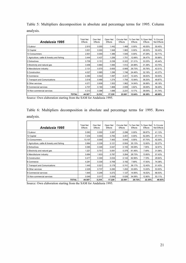
Table 5: Multipliers decomposition in absolute and percentage terms for 1995. Column

Source: Own

analysis.

elaboration starting from the SAM for Andalusia 1995.

able 6: Multipliers decomposition in absolute and percentage terms for 1995. Rows


Own Net Effects

Open Net Effects


% Own Net Effects

% Open Net Effects


11Labour 2.910 0.000 1.442 1.468 0.00% 49.55% 50.45%

12 Capital 3.931 0.000 1.948 1.983 0.00% 49.55% 50.45%

13 Consummers 2.931 0.000 1.386 1.545 0.00% 47.29% 52.71%


2 Extractives 0.709 0.151 0.236 0.322 21.31% 33.25% 45.44%



5 Construction 4.027 0.985 1.296 1.746 24.46% 32.18% 43.37%

6 Commerce 4.360 0.542 1.597 2.221 12.44% 36.63% 50.93%


8 Other services 4.071 0.608 1.502 1.962 14.94% 36.88% 48.18%



TOTAL 44.507 5.218 17.229 22.061 12.64% 38.38% 48.98%

T

analysis.

Source: Own elaboration starting from the SAM for Andalusia 1995.

Andalusia 1995 Effects Effects Effects Effects Effects Effects Net Effects

11Labour 5.583 0.000 3.287 2.296 0.00% 58.87% 41.13%

12 Capital 7.234 0.000 3.783 3.451 0.00% 52.29% 47.71%

13 Consummers 13.107 0.000 7.563 5.544 0.00% 57.70% 42.30%


2 Extractives 0.585 0.346 0.047 0.193 59.08% 7.95% 32.97%



5 Construction 0.477 0.300 0.034 0.142 62.96% 7.19% 29.84%

6 Commerce 4.291 0.330 0.769 3.192 7.69% 17.93% 74.38%


8 Other services 2.229 0.737 0.290 1.202 33.06% 13.00% 53.93%


10 Non-commercial services 0.049 0.017 0.006 0.026 34.08% 12.80% 53.11%TOTAL 44.507 5.218 17.229 22.061 28.72% 22.35% 48.93%

Total Net Own Net Open Net Circular Net % Own Net % Open Net % Circular

21

Table 7: Multipliers decomposition in absolute and percentage terms for 1999. Columns

analysis.


Own Net Effects

Open Net Effects


% Own Net Effects

% Open Net Effects


11Labour 3.686 0.000 1.741 1.945 0.00% 47.23% 52.77%

12 Capital 3.686 0.000 1.741 1.945 0.00% 47.23% 52.77%

13 Consummers 2.686 0.000 1.156 1.530 0.00% 43.04% 56.96%


2 Extractives 0.573 0.115 0.195 0.263 20.12% 34.09% 45.79%



5 Construction 3.186 0.358 1.207 1.621 11.25% 37.87% 50.88%

6 Commerce 3.791 0.172 1.544 2.074 4.54% 40.74% 54.72%


8 Other services 2.921 0.177 1.171 1.573 6.06% 40.09% 53.85%



TOTAL 37.294 2.297 15.281 19.716 7.81% 40.07% 52.12%


Table 8: Multipliers decomposition in absolute and percentage terms for 1999. Rows

analysis.

Andalusia 1999 Efectos Netos

Totales

Efectos Netos

Propios

Efectos Netos

abiertos

Efectos Netos

Circulares% EN

Propios% EN

Abiertos% EN

Circulares

11Labour 3.906 0.000 2.136 1.770 0.00% 54.69% 45.31%

12 Capital 7.321 0.000 3.600 3.721 0.00% 49.18% 50.82%

13 Consummers 13.227 0.000 7.321 5.906 0.00% 55.35% 44.65%


2 Extractives 0.224 0.175 0.010 0.038 78.21% 4.59% 17.19%



5 Construction 0.230 0.141 0.019 0.070 61.35% 8.15% 30.50%

6 Commerce 3.186 0.144 0.641 2.401 4.53% 20.13% 75.34%


8 Other services 2.738 0.328 0.508 1.901 11.99% 18.56% 69.45%



TOTAL 37.294 2.297 15.281 19.716 22.88% 23.64% 53.48%


22

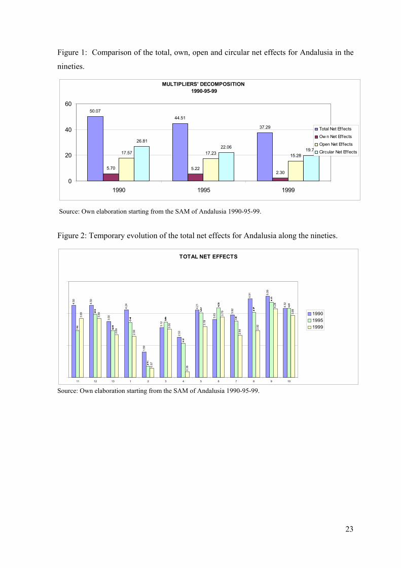
Figure 1: Comparison of the total, own, open and circular net effects for Andalusia in the

nineties.

MULTIPLIERS' DECOMPOSITION 1990-95-99

50.0744.51

37.29

5.70 5.222.30

17.57 17.23 15.28

26.8122.06 19.72

0

20

40

60

1990 1995 1999

Total Net Effects

Ow n Net Effects

Open Net Effects


Source: Own elaboration starting from the SAM of Andalusia 1990-95-99.

Figure 2: Temporary evolution of the total net effects for Andalusia along the nineties.

6

4

2

0

TOTAL NET EFFECTS

4.50

3.50

4.24

1.59

3.12

2.53

4.21

3.63

3.92

4.91 5.

09

4.32

3.69

3.69

2.69

2.59

0.57

3.00

0.36

3.19

3.79

2.64

2.92

4.28

3.89

4.50

11 12 13 1 2 3 4 5 6 7 8 9 10

199019951999


23

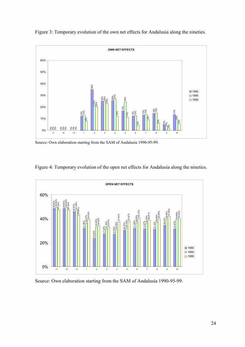
Figure 3: Temporary evolution of the own net effects for Andalusia along the nineties.

OWN NET EFFECTS0% 0% 0%

12%

35%

25%

26%

17%

12% 13% 14

%

5%

13%

0% 0% 0%

13%

21%

25% 27

%

24%

12% 14

% 15%

4%

9%

0% 0% 0%

8%

20% 23

%

12%

11%

5%

9%

6%

2%

6%

0%

10%

20%

30%

40%

50%

60%

11 12 13 1 2 3 4 5 6 7 8 9 10

199019951999


Figure 4: Temporary evolution of the open net effects for Andalusia along the nineties.

OPEN NET EFFECTS

48.6

4%

48.6

4%

45.9

7%

31.9

6%

23.6

0% 27.2

5%

27.0

4% 30.3

3%

31.9

0%

31.5

7%

31.1

0% 34.4

7%

31.4

7%

49.5

5%

49.5

5%

47.2

9%

36.4

7%

33.2

5%

31.3

8%

30.7

6%

32.1

8% 36.6

3%

36.2

0%

36.8

8% 39.6

9%

39.0

9%

47.2

3%

47.2

3%

43.0

4%

39.3

5%

34.0

9%

32.8

7% 37.4

4%

37.8

7% 40.7

4%

38.8

1%

40.0

9%

41.9

3%

40.2

2%

0%

20%

40%

60%

11 12 13 1 2 3 4 5 6 7 8 9 10

199019951999


24

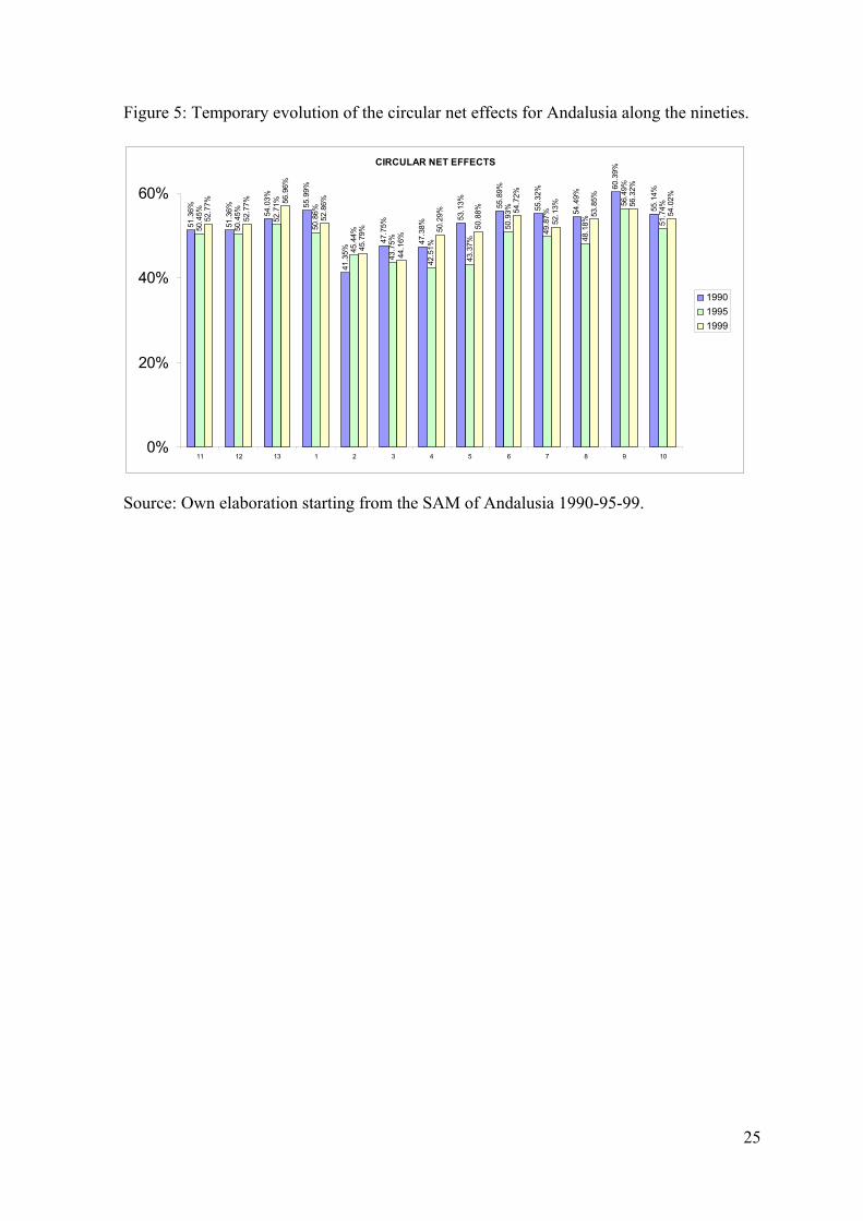
Figure 5: Temporary evolution of the circular net effects for Andalusia along the nineties.

CIRCULAR NET EFFECTS

51.3

6%

51.3

6% 54.0

3%

55.9

9%

41.3

5%

47.7

5%

47.3

8%

53.1

3% 55.8

9%

55.3

2%

54.4

9%

60.3

9%

55.1

4%

50.4

5%

50.4

5%

52.7

1%

50.8

6%

45.4

4%

43.7

5%

42.5

1%

43.3

7%

50.9

3%

49.8

7%

48.1

8%

56.4

9%

51.7

4%

52.7

7%

52.7

7% 56.9

6%

52.8

6%

45.7

9%

44.1

6%

50.2

9%

50.8

8% 54.7

2%

52.1

3%

53.8

5% 56.3

2%

54.0

2%

0%

20%

40%

60%

11 12 13 1 2 3 4 5 6 7 8 9 10

199019951999


25

Table 9: Employment multipliers for Andalusia in 1990.

Accounts1 0.950 0.023 0.049 0.116 0.095 0.092 0.080 0.094 0.099 0.087 0.108 0.108 0.108 2.008 0.154 0.091 1.6992 0.002 0.028 0.007 0.002 0.002 0.002 0.003 0.002 0.002 0.002 0.002 0.002 0.002 0.058 0.004 0.0493 0.004 0.002 0.079 0.003 0.004 0.004 0.004 0.005 0.005 0.006 0.004 0.004 0.004 0.129 0.010 0.1094 0.074 0.019 0.036 0.173 0.089 0.059 0.069 0.068 0.071 0.070 0.075 0.075 0.075 0.951 0.073 0.8055 0.016 0.007 0.015 0.009 0.413 0.015 0.015 0.020 0.022 0.021 0.020 0.020 0.020 0.611 0.047 0.5176 0.233 0.068 0.153 0.131 0.233 0.795 0.200 0.243 0.272 0.234 0.291 0.291 0.291 3.437 0.264 2.9077 0.036 0.017 0.028 0.023 0.039 0.033 0.245 0.039 0.041 0.040 0.038 0.038 0.038 0.657 0.051 0.5558 0.024 0.010 0.018 0.016 0.028 0.026 0.026 0.221 0.039 0.042 0.030 0.030 0.030 0.539 0.041 0.4569 0.060 0.026 0.038 0.031 0.056 0.065 0.055 0.074 0.609 0.061 0.076 0.076 0.076 1.303 0.100 1.102

10 0.003 0.002 0.001 0.001 0.001 0.001 0.001 0.002 0.002 2.108 0.002 0.002 0.002 2.128 0.164 1.800Sum of columns 1.402 0.202 0.426 0.503 0.961 1.093 0.699 0.766 1.162 2.670 0.646 0.646 0.646Average value 0.140 0.020 0.043 0.050 0.096 0.109 0.070 0.077 0.116 0.267 0.065 0.065 0.065Total average 0.091Normalized value 1.542 0.222 0.468 0.553 1.057 1.202 0.769 0.842 1.278 2.936 0.710 0.710 0.710

139 10 11 125 6 7 81 2 3 4 Normaliz. value

Total average

Average value

Sum of row

Source: Own elaboration through SAM for Andalusia 1990.

26


Accounts1 0.598 0.006 0.023 0.072 0.046 0.042 0.031 0.033 0.037 0.038 0.028 0.038 0.038 1.033 0.079 0.072 1.1012 0.004 0.130 0.023 0.009 0.007 0.004 0.003 0.004 0.004 0.004 0.003 0.004 0.004 0.200 0.015 0.2133 0.003 0.001 0.060 0.002 0.002 0.003 0.002 0.003 0.003 0.003 0.002 0.002 0.002 0.086 0.007 0.0924 0.036 0.007 0.024 0.106 0.058 0.041 0.033 0.034 0.036 0.033 0.026 0.036 0.036 0.506 0.039 0.5395 0.004 0.001 0.002 0.001 0.171 0.004 0.002 0.003 0.004 0.005 0.002 0.003 0.003 0.206 0.016 0.2196 0.131 0.024 0.105 0.068 0.131 0.584 0.137 0.138 0.179 0.160 0.141 0.191 0.191 2.179 0.168 2.3237 0.023 0.010 0.023 0.019 0.033 0.042 0.313 0.028 0.030 0.028 0.020 0.027 0.027 0.624 0.048 0.6658 0.019 0.005 0.021 0.014 0.024 0.032 0.025 0.226 0.031 0.041 0.021 0.028 0.028 0.514 0.040 0.5489 0.099 0.027 0.092 0.057 0.110 0.166 0.114 0.147 1.135 0.166 0.116 0.157 0.157 2.543 0.196 2.711

10 0.004 0.001 0.003 0.002 0.003 0.004 0.003 0.006 0.005 1.444 0.004 0.005 0.005 1.489 0.115 1.587Sum of columns 0.920 0.212 0.376 0.350 0.587 0.922 0.664 0.621 1.462 1.921 0.363 0.491 0.491Average value 0.092 0.021 0.038 0.035 0.059 0.092 0.066 0.062 0.146 0.192 0.036 0.049 0.049Total average value 0.072Normalized value 1.275 0.294 0.521 0.485 0.813 1.278 0.921 0.860 2.026 2.662 0.504 0.680 0.680

Average value

Total average

Normaliz. value11 12 13 Sum of

row7 8 9 103 4 5 61 2

Source: Own elaboration through SAM for Andalusia 1995.

27


ource: Own elaboration through SAM for Andalusia 1999.

Accounts1 1.157 0.004 0.020 0.013 0.026 0.035 0.021 0.024 0.037 0.039 0.040 0.040 0.040 1.499 0.115 0.140 0.8232 0.003 0.628 0.082 0.003 0.007 0.004 0.003 0.003 0.004 0.004 0.004 0.004 0.004 0.752 0.058 0.4133 0.002 0.001 0.081 0.000 0.002 0.003 0.002 0.002 0.003 0.003 0.003 0.003 0.003 0.110 0.008 0.0604 0.209 0.057 0.155 1.352 0.341 0.209 0.186 0.146 0.195 0.191 0.200 0.200 0.200 3.640 0.280 1.9995 0.004 0.001 0.003 0.000 0.313 0.003 0.002 0.002 0.004 0.006 0.003 0.003 0.003 0.347 0.027 0.1916 0.232 0.047 0.213 0.029 0.264 1.449 0.241 0.244 0.371 0.341 0.406 0.406 0.406 4.647 0.357 2.5527 0.024 0.014 0.029 0.004 0.033 0.042 0.481 0.026 0.037 0.035 0.038 0.038 0.038 0.838 0.064 0.4608 0.048 0.011 0.054 0.007 0.061 0.079 0.055 0.403 0.087 0.096 0.091 0.091 0.091 1.173 0.090 0.6449 0.153 0.040 0.157 0.021 0.188 0.254 0.166 0.191 1.501 0.272 0.298 0.298 0.298 3.836 0.295 2.107

10 0.011 0.002 0.011 0.001 0.013 0.016 0.011 0.013 0.019 1.205 0.021 0.021 0.021 1.365 0.105 0.750Sum of columns 1.844 0.805 0.803 1.430 1.248 2.096 1.169 1.054 2.257 2.193 1.102 1.102 1.102Average value 0.184 0.081 0.080 0.143 0.125 0.210 0.117 0.105 0.226 0.219 0.110 0.110 0.110Total average value 0.140Normalized value 1.317 0.575 0.573 1.021 0.891 1.496 0.834 0.753 1.612 1.566 0.787 0.787 0.787

Normaliz. value13 Sum of

rowAverage

valueTotal

average9 10 11 125 6 7 81 2 3 4

S

28

Documents

Multiplier decomposition within Regional SAMs: the case of Andalusia