Multiscale approximation of the solution of weakly singular second kind Fredholmintegral equation in Legendre Multiwavelet basis

Swaraj Paul 1, M. M. Panja 1 and B. N. Mandal 2

1 Department of MathematicsVisva-Bharati, Santiniketan-731235

West Bengal, Indiae-mail: madanpanja2005@yahoo.co.in

2 Physics and Applied Mathematics Unit,Indian Statistical Institute

203, B T Road, Kolkata 700108, Indiae-mail: birenisical@gmail.com

Abstract

Numerical solution of Fredholm integral equation of second kind with weakly singular kernel is obtained in thispaper by employing Legendre multi-wavelet basis. The low- and high-pass filters for two-scale relations involvingLegendre multiwavelets having four or five vanishing moments of their wavelets have been derived and are usedin the evaluation of integrals for the multiscale representation of the integral operator. Explicit expressions forthe elements of the matrix associated with the multiscale representation are given. An estimate for the Holderexponent of the solution of the integral equation at any point in its domain is obtained. A number of examplesis provided to illustrate the efficiency of the method developed here.

Keywords: Legendre multiwavelet, Fredholm integral equation of second kind with weakly singular kernel,wavelet Galerkin method, Multiscale approximation.

AMS subject classification: 65N38, 65N55, 65R20, 65D15

1 Introduction

Integral equations arise in various problems of mathematical physics in a natural way and as such they play im-portant role in varieties of field of science and engineering [1–3]. Fredholm integral equation of the second kindwith regular or singular kernels constitute an important branch in such area. Investigations on mathematicaltechniques for getting exact solution of such equations have been continued for a long time and reported in anumber of literature [4–7]. However, such results are not adequate for getting solutions of integral equations ap-pearing in several types of physical problems. Thus, investigations are continued simultaneously to find efficientapproximation schemes which can provide approximate solution as accurate as possible. There already existseveral numerical schemes for getting approximate solution of integral equations with singular kernels [8–19].But in most of the cases the unknown function involved in the equation is expanded in some orthogonal basesso as to reduce the integral equation to a system of linear simultaneous equation for the unknown coefficientsappearing in the truncated expansion of the function. However the matrices involved in the system of linearequations are dense and their condition numbers are high, in general. As a result their computational costare prohibitive. Also the approximate solution when expanded in the basis consisting of classical orthogonalfunctions, often fails to provide local informations such as smoothness or regularity of the solutions, the errorin the approximation in a straight forward manner. It is thus desirable to search for an appropriate techniquewhich can provide the information on the aforesaid local behaviour or error in the approximation directly fromthe solution of the transferred algebraic equations at the expense of the less computational cost. It is nowknown that the use of wavelet basis of some multiresolution analysis(MRA) of underlying space of functions inapproximating solution of integral equations can provide such informations efficiently [20–27].

Multiresolution analysis (MRA) of function spaces in terms of refinable functions and wavelets with compactsupport has significant applications in many areas of mathematical physics and engineering [28–32]. This canbe attributed due to its elegant role of mathematical microscopy in the analysis of smoothness or regularity of afunction. The main advantages of a numerical method involving expansion of the unknown function in terms ofwavelets with compact support compared to a classical method are that discretization of the domain involved

1

is inbuilt in the technique due to the compact support of the members in the basis and the resulting matrix issparse due to vanishing moments of the wavelets. Consequently the numerical scheme involving basis of MRAbecomes highly stable and the related computation is economic.

Alpert [20], Alpert et al. [21] are pioneers in the development of generation of wavelets involving polyno-mials and they used these to obtain numerical solutions of second kind integral equations with emphasis onlogarithmically singular kernels. In recent years, several numerical methods for obtaining numerical solution ofa Fredholm integral equation of the form

u(x) + λ

∫ 1

0

u(t)

|x− t|µdt = f(x), 0 < µ < 1, x ∈ [0, 1] (1.1)

where f : [0, 1]→ R is the input function(known) and u is the output function(unknown), have been developedby a number of researchers [10,20,21,33–37]. Cai [37] observed that all existing numerical methods for solvingweakly singular integral equations are of two types. In the first type, the integral equation is converted intoa new but somewhat complicated integral equation possessing better regularity so as to be treated by someappropriate existing method [34]. The second type is called a hybrid projection method which allows the pro-jection subspaces to contain some known singular functions [10, 22]. This method requires a special attentionfor the evaluation of integrals involving singular functions in the basis. Since the basis (with compact support)of MRA of function spaces have inherent structure of regularization of singular functions, it is quite naturalto investigate whether numerical solution of singular integral equation in the wavelet basis can achieve someadditional benefits compared to existing classical methods.

In this paper Legendre multiwavelets have been used to solve a second kind Fredholm integral equationwith weakly singular kernel. Definition of Legendre multiwavelets, their two-scale relations and associated filtercoefficients are given in section 2. Section 3 involves recurrence relations for integrals involving product of weaklysingular kernels, scale functions and wavelets, some representative values of these integrals are also presented.Section 4 presents multiscale approximation of a function and multiscale representation of the weakly singularintegral operator. In section 5, the second kind integral equation is reduced to a linear system of algebraicequations involving multiscale representation of the integral operator and an estimate for Holder exponent ofthe solution at any point within the domain is obtained. An error estimate for the approximate solution isobtained in section 6. The numerical method developed here is illustrated through a number of examples insection 7. Finally in section 8 we present some concluding remarks including possible extension of the schemeto some other mathematical problems.

2 Legendre multiwavelets

The scaling functions in Legendre multiwavelet bases consist of K component vectors

φi(x) := (2i+ 1)12Pi(2x− 1), i = 0, 1, ...,K − 1; 0 ≤ x ≤ 1 (2.1)

where Pi(x) is the Legendre polynomial of degree i (i = 0, 1, ...,K − 1). At resolution j these are expressed as

φij,k(x) := 2j2φi(2jx− k), j ∈ N (2.2)

where, N = {0, 1, 2, ...} and supp φij,k(x) =[k2j ,

k+12j

). For a given j > 0, shifting or translation of φij,k(x) is

represented by the symbol k(k = 0, 1, ..., 2j − 1

). In a particular resolution j, φi1j,k1(x) is orthogonal to φi2j,k2(x)

for i1 6= i2, k1 6= k2 with respect to the inner product < f, g >=∫ 1

0f(x)g(x)dx. Apart from the usual recurrence

relation (in n) for Pn(x)(viz. (n+ 1)Pn+1(x)− (2n+ 1)x Pn(x) + n Pn−1(x) = 0), the refinement equations orthe two-scale relations among the scale functions φij,k(x) are

φij,k(x) =1√2

K−1∑r=0

(h

(0)i,r φ

rj+1,2k(x) + h

(1)i,r φ

rj+1,2k+1(x)

)=

1√2

K−1∑r=0

1∑s=0

h(s)i,rφ

rj+1,2k+s(x). (2.3)

The elements h(s)i,r (s = 0, 1) of the low-pass filter H = 1√

2

(h(0)

... h(1)

)are determined uniquely by using the

definition (2.1) into (2.3) and the formula [38]

h(0)i,j =

K−1∑m=0

ωmφi(xm

2

)φj (xm) (2.4)

2

h(1)i,j = (−1)i+jh

(0)i,j . (2.5)

Here xm and ωm are nodes and weights for Gauss-Legendre quadrature formula in (0, 1).

The elements ψij,k(x)(

:= 2j2ψi(2jx− k)

)of Legendre multiwavelets ψj,k having K components for each j and

admissible k are given by

ψij,k(x) =1√2

K−1∑r=0

(g

(0)i,r φ

rj+1,2k(x) + g

(1)i,r φ

rj+1,2k+1(x)

)=

1√2

K−1∑r=0

1∑s=0

g(s)i,r φ

rj+1,2k+s(x). (2.6)

The elements g(s)i,r (s = 0, 1) of the high-pass filter G = 1√

2

(g(0)

... g(1)

)are obtained by using the following

relations at resolution 0 [35] :∫ 1

0

ψi0,0(x)xmdx = 0 for i = 0, 1, ...,K − 1; m = 0, 1, ...,K − 1 + i , (2.7)∫ 1

0

ψi10,0(x)ψi20,0(x)dx = δi1,i2 for i1, i2 = 0, 1, ...,K − 1. (2.8)

Explicit values of the elements of h(0),g(0) for K = 4 are

h(0) =

1 0 0 0

−√

32

12 0 0

0 −√

154

14 0

√7

8

√218 −

√358

18

,g(0) =

0 2√85

2√

317 −

√2185

− 1√21

− 1√7

− 12

√521

√3

2

0 − 14

√2185 − 3

4

√717 − 8√

85

58

√521

58

√57

238√

21

√158

(2.9)

while for K = 5

h(0) =

1 0 0 0 0

−√

32

12 0 0 0

0 −√

154

14 0 0

√7

8

√218 −

√358

18 0

0√

38

3√

58 − 3

√7

16116

, (2.10)

g(0) =

− 2√93

− 2√31

− 5√93

√2131 −

√331

0 − 14

√319 − 3

4

√519 −

√719

3√19

52

√35

734752

√35

244967√

51429−√

152449 −30

√15

17143

0 − 18

√719 − 1

8

√10519 − 25

16

√319 − 11

16

√2119

− 78

√779 − 7

8

√2179 − 47

8

√5

533 − 398√

79− 8√

553

. (2.11)

The elements g(1)i,j of g(1) can be found from the elements of g(0) by using the formulae (cf. equation(3.27)

in [38])

g(1)i,j = (−1)

i+j+Kg

(0)i,j . (2.12)

3

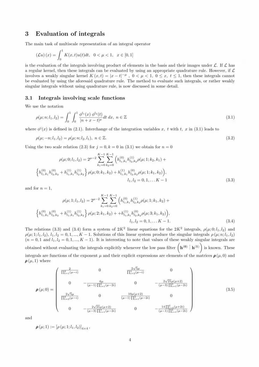
3 Evaluation of integrals

The main task of multiscale representation of an integral operator

(Lu) (x) =

∫ 1

0

K(x, t)u(t)dt, 0 < µ < 1, x ∈ [0, 1]

is the evaluation of the integrals involving product of elements in the basis and their images under L. If L hasa regular kernel, then these integrals can be evaluated by using an appropriate quadrature rule. However, if Linvolves a weakly singular kernel K (x, t) = |x − t|−µ , 0 < µ < 1, 0 ≤ x, t ≤ 1, then these integrals cannotbe evaluated by using the aforesaid quadrature rule. The method to evaluate such integrals, or rather weaklysingular integrals without using quadrature rule, is now discussed in some detail.

3.1 Integrals involving scale functions

We use the notation

ρ(µ;n; l1, l2) =

∫ 1

0

∫ 1

0

φl1(x) φl2(t)

|n+ x− t|µdt dx, n ∈ Z (3.1)

where φi(x) is defined in (2.1). Interchange of the integration variables x, t with t, x in (3.1) leads to

ρ(µ;−n; l1, l2) = ρ(µ;n; l2, l1), n ∈ Z. (3.2)

Using the two scale relation (2.3) for j = 0, k = 0 in (3.1) we obtain for n = 0

ρ(µ; 0; l1, l2) = 2µ−2K−1∑k1=0

K−1∑k2=0

(h

(0)l1,k1

h(1)l2,k2

ρ(µ; 1; k2, k1) +{h

(0)l1,k1

h(0)l2,k2

+ h(1)l1,k1

h(1)l2,k2

}ρ(µ; 0; k1, k2) + h

(1)l1,k1

h(0)l2,k2

ρ(µ; 1; k1, k2)),

l1, l2 = 0, 1, . . .K − 1 (3.3)

and for n = 1,

ρ(µ; 1; l1, l2) = 2µ−2K−1∑k1=0

K−1∑k2=0

(h

(0)l1,k1

h(1)l2,k2

ρ(µ; 1; k1, k2) +{h

(0)l1,k1

h(0)l2,k2

+ h(1)l1,k1

h(1)l2,k2

}ρ(µ; 2; k1, k2) + +h

(1)l1,k1

h(0)l2,k2

ρ(µ; 3; k1, k2)),

l1, l2 = 0, 1, . . .K − 1. (3.4)

The relations (3.3) and (3.4) form a system of 2K2 linear equations for the 2K2 integrals, ρ(µ; 0; l1, l2) andρ(µ; 1; l1, l2), l1, l2 = 0, 1, ...,K − 1. Solutions of this linear system produce the singular integrals ρ (µ;n; l1, l2)(n = 0, 1 and l1, l2 = 0, 1, ...,K − 1). It is interesting to note that values of these weakly singular integrals are

obtained without evaluating the integrals explicitly whenever the low pass filter

(h(0)

... h(1)

)is known. These

integrals are functions of the exponent µ and their explicit expressions are elements of the matrices ρρρ (µ, 0) andρρρ (µ, 1) where

ρρρ (µ; 0) =

2∏2i=1(µ−i) 0 2

√5µ∏4

i=2(µ−i) 0

0 − 6µ(µ−1)

∏2i=1(µ−2i)

0 − 2√

21µ(µ+2)

(µ−3)∏3i=1(µ−2i)

2√

5µ∏4i=2(µ−i) 0 10µ(µ+2)

(µ−1)∏3i=1(µ−2i)

0

0 − 2√

21µ(µ+2)

(µ−3)∏3i=1(µ−2i)

0 − 14∏2i=0(µ+2i)

(µ−1)∏4i=1(µ−2i)

(3.5)

and

ρρρ (µ; 1) := [ρ (µ; 1; l1, l2)]4×4 ,

4

with

ρ (µ; 1; 0, 0) =22−µ − 2∏2i=1 (µ− i)

, ρ (µ; 1; 0, 1) = −ρ (µ; 1; 1, 0) =

√3{4− 22−µ (1 + µ)}∏3

i=1 (µ− i),

ρ (µ; 1; 0, 2) = ρ (µ; 1; 2, 0) =

√5{22−µ (12 + 5µ+ µ2

)− 2

(24− 7µ+ µ2

)}∏4

i=1 (µ− i),

ρ (µ; 1; 0, 3) = −ρ (µ; 1; 3, 0) =4√

7{6(30− 9µ+ µ2

)− 2−µ (5 + µ)

(36 + 7µ+ µ2

)}∏5

i=1 (µ− i),

ρ (µ; 1; 1, 1) = −6{8− 7µ+ µ2 − 21−µ (4− µ− µ2

)}∏4

i=1 (µ− i),

ρ (µ; 1; 1, 2) = −ρ (µ; 1; 2, 1) =

√15{8

(14− 9µ+ µ2

)− 22−µ (28 + µ− 4µ2 − µ3

)}∏5

i=1 (µ− i),

ρ (µ; 1; 1, 3) = ρ (µ; 1; 3, 1) =

√21{22−µ (600 + 46µ− 35µ2 − 10µ3 − µ4

)− 2

(1200− 738µ+ 155µ2 − 18µ3 + µ4

)}∏6

i=1 (µ− i),

ρ (µ; 1; 2, 2) =5{22−µ (72− 54µ− µ2 + 6µ3 + µ4

)− 288 + 420µ− 214µ2 + 36µ3 − 2µ4}∏6

i=1 (µ− i),

ρ (µ; 1; 2, 3) = −ρ (µ; 1; 3, 2)

=

√35{22−µ (−1224 + 438µ+ 107µ2 − 29µ3 − 11µ4 − µ5

)+ 4896− 5160µ+ 1956µ2 − 264µ3 + 12µ4}∏7

i=1 (µ− i),

ρ (µ; 1; 3, 3) = 7{22−µ (2880− 2904µ+ 710µ2 + 111µ3 − 61µ4 − 15µ5 − µ6)−

11520 + 19536µ− 13700µ2 + 5022µ3 − 842µ4 + 66µ5 − 2µ6}/8∏i=1

(µ− i) . (3.6)

The integrals ρ (µ;n; l1, l2) for n ≥ 2 are not singular and hence can be evaluated by an appropriate quadraturerule without any difficulty. Their expressions for l1, l2 = 0, 1, ...,K − 1 (K = 4) are obtained but not given here.

3.2 Integrals involving product of scale functions and wavelets

We use the notation

α(µ;n; l1; l2, j, k) =

∫ 1

0

∫ 1

0

φl1(x) ψl2j,k(t)

|n+ x− t|µdt dx, n ∈ Z , j ≥ 0, k = 0, 1, .., 2j − 1. (3.7)

By using the relations (2.3) and (2.6) for j = 0 in (3.7) and after some algebraic simplifications we obtain

α(µ;n; l1; l2, 0, 0) = 2µ−2K−1∑k1=0

K−1∑k2=0

({h

(0)l1,k1

g(0)l2,k2

+ h(1)l1,k1

g(1)l2,k2

}ρ(µ; 2n; k1, k2) +

h(0)l1,k1

g(1)l2,k2

ρ(µ; 2n− 1; k1, k2) + h(1)l1,k1

g(0)l2,k2

ρ(µ; 2n+ 1; k1, k2)). (3.8)

The values of ρ(µ; 0; k1, k2) and ρ(µ; 1; k1, k2) appearing in (3.8) have already been obtained in (3.5), (3.6) andρ(µ;−1; k1, k2)’s can be evaluated by using the formula given in (3.2) .The formula for the evaluation of α(µ;n; l1; l2, j, k) for j > 0 and k = 0, 1, ..., 2j − 1 is given by

α(µ;n; l1; l2, j, k) =

2µ−32

∑K−1k1=0{h

(0)l1k1

α(µ; 2n; k1; l2, j − 1, k) + h(1)l1k1

α(µ; 2n+ 1; k1; l2, j − 1, k)},

for k = 0, 1, . . . 2j−1 − 1,

2µ−32

∑K−1k1=0{h

(0)l1k1

α(µ; 2n− 1; k1; l2, j − 1, k − 2j−1)+

h(1)l1k1

α(µ; 2n; k1; l2, j − 1, k − 2j−1)},

for k = 2j−1, 2j−1 + 1, . . . 2j − 1.

(3.9)

5

If we use the notation

β(µ;n; l1, j, k; l2) =

∫ 1

0

∫ 1

0

ψl1j,k(x) φl2(t)

|n+ x− t|µdt dx, n ∈ Z , j ≥ 0, k = 0, 1, .., 2j − 1, (3.10)

then these integrals can be evaluated by using the relation

β (µ;n; l1, j, k; l2) := α (µ;−n; l2; l1, j, k) . (3.11)

3.3 Integrals involving product of wavelets

Here we use the notation

γ(µ;n; l1, j1, k1; l2, j2, k2) =

∫ 1

0

∫ 1

0

ψl1j1,k1(x) ψl2j2,k2(t)

|n+ x− t|µdt dx, n ∈ Z, j1, j2 ∈ N,

k1 = 0, 1, .., 2j1 − 1, k2 = 0, 1, .., 2j2 − 1 (3.12)

which involves integration of product of Legendre multiwavelets.When j1 = j2 = 0, γ (µ;n; l1, 0, 0; l2, 0, 0) can be expressed as

γ(µ;n; l1, 0, 0; l2, 0, 0) = 2µ−2K−1∑k1=0

K−1∑k2=0

({g

(0)l1,k1

g(0)l2,k2

+ g(1)l1,k1

g(1)l2,k2

}ρ(µ; 2n; k1, k2) +

g(0)l1,k1

g(1)l2,k2

ρ(µ; 2n− 1; k1, k2) + g(1)l1,k1

g(0)l2,k2

ρ(µ; 2n+ 1; k1, k2))

(3.13)

so that these integrals are now obtained since ρ’s are known from section 3.1.

Again, when j1 = 0 (so that k1 = 0) in (3.12), then γ (µ;n; l1, 0, 0; l2, j, k) can be expressed as

γ(µ;n; l1, 0, 0; l2, j, k) =

2µ−32

∑K−1k1=0{g

(0)l1k1

α(µ; 2n; k1; l2, j − 1, k) + g(1)l1k1

α(µ; 2n+ 1; k1; l2, j − 1, k)},

for k = 0, 1, . . . 2j−1 − 1,

2µ−32

∑K−1k1=0{g

(0)l1k1

α(µ; 2n− 1; k1; l2, j − 1, k − 2j−1)+

g(1)l1k1

α(µ; 2n; k1; l2, j − 1, k − 2j−1)},

for k = 2j−1, 2j−1 + 1, . . . 2j − 1

(3.14)

so that these integrals are now obtained since α’s appearing in (3.14) are known from section 3.2.

Finally, when n = 0, 0 < j1 < j2, k1 = 0, 1, ..., 2j1 − 1 and k2 = 0, 1, ..., 2j2 − 1,

γ (µ; 0; l1, j1, k1; l2, j2, k2) = 2j1(µ−1)γ(µ; k1 − r; l1, 0, 0; l2, j2 − j1, k2 − 2j2−j1r

)(3.15)

where r takes up a value in 0, 1, ..., 2j − 1 such that k2 ∈ {r2j2−j1 , r2j2−j1 + 1, ..., (r + 1)2j2−j1 − 1}, so thatthese integrals also become now known.

We now denote the matrices with sizes as

ρρρ (µ) := [ρ (µ; 0; l1, l2)]K×K ,

ααα (µ; j) := [α (µ; 0; l1; l2, j, k)]K×(2jK) ,

βββ (µ; j) := [β (µ; 0; l1, j, k; l2)](2jK)×K ,

γγγ (µ; j1, j2) := [γ (µ; 0; l1, j1, k1; l2, j2, k2)](2j1K)×(2j2K) . (3.16)

6

4 Multiscale approximation

Here we utilize the results obtained in section 3 to obtain multiscale approximation and representation of afunction f ∈ L2[0, 1] and the integral operator L. The projection of f into the approximation space V KJ (thelinear span of φlJ,k(x), l = 0, 1, . . . ,K − 1, k = 0, 1, . . . 2J − 1) is [38]

f(x) ≈ (PV KJ f)(x) ≡2J−1∑k=0

K−1∑l=0

clJ,k φlJ,k(x). (4.1)

Its projection (decomposition) into the approximation space V K0 and detail spaces WKj (0 ≤ j ≤ J − 1) is given

by

f(x) ≈

PV K0

⊕(J−1⊕j=0

WKj )f

(x) =

K−1∑l=0

{cl0,0 φ

l(x) +

J−1∑j=0

2j−1∑k=0

dlj,k ψlj,k(x)

}(4.2)

where the notation c and d are used to denote the coefficients of scale function and wavelet in the multiscaleexpansion of f . At this stage we introduce the following notations for convenience. For a given j and k =0, 1, . . . 2j − 1

Φj,k(x) =(φ0j,k(x), φ1

j,k(x), . . . φK−1j,k (x)

), (4.3)

Ψj,k(x) =(ψ0j,k(x), ψ1

j,k(x), . . . ψK−1j,k (x)

). (4.4)

The bases for V KJ , WKj and

J⊕j=0

WKj are then denoted by

ΦJ :=(ΦJ,0(x),ΦJ,1(x), . . .ΦJ,2J−1(x)

)(4.5)

which is a vector having 2JK components,

Ψj :=(Ψj,0(x),Ψj,1(x), . . .Ψj,2j−1(x)

)(4.6)

which is a vector having 2jK components, and

JΨ := (Ψ0,Ψ1, . . .ΨJ) (4.7)

which is a vector having (2J+1 − 1)K components.

Also we use the symbols

cJ,k :=

(∫ k+1

2J

k

2J

f(x)φ0J,k(x)dx,

∫ k+1

2J

k

2J

f(x)φ1J,k(x)dx, · · · ,

∫ k+1

2J

k

2J

f(x)φK−1J,k (x)dx

), k = 0, 1, .., 2J − 1, (4.8)

dj,k :=

(∫ k+1

2j

k

2j

f(x)ψ0j,k(x)dx,

∫ k+1

2j

k

2j

f(x)ψ1j,k(x)dx, · · · ,

∫ k+1

2j

k

2j

f(x)ψK−1j,k (x)dx

), k = 0, 1, .., 2j − 1. (4.9)

The components of cJ,k and dj,k are the coefficients in multiscale approximation of f(x) in the approximationspace V KJ and the detail space WK

j respectively. Finally we use the symbols

cJ :=(cJ,0, cJ,1, . . . cJ,2J−1

)(4.10)

which is a vector having 2JK components,

dj :=(dj,0,dj,1, . . .dj,2j−1

)(4.11)

which is vector having 2jK components, and

Jd := (d0,d1, . . .dJ) (4.12)

7

which is vector having (2J+1 − 1)K components. Then (4.1) and (4.2) can be expressed as [35](PV KJ f

)(x) = ΦJ cTJ (4.13)

and PV K0

⊕(J−1⊕j=0

WKj

)f (x) = (Φ0, (J−1)Ψ)

cT0

(J−1)dT

(4.14)

where the superscript T denotes the transpose.

Let the integral operator L be defined by

(Lu) (x) =

∫ 1

0

u(t)

|x− t|µdt, 0 < µ < 1, x ∈ [0, 1]. (4.15)

Then (Lφl1

)(x) =

∫ 1

0

φl1(t)

|x− t|µdt

=K−1∑l2=0

ρ(µ; 0; l1, l2)φl2(x) +

J−1∑j2=0

2j2−1∑k2=0

β(µ; 0; l2, j2, k2; l1)ψl2j2,k2(x)

,

(4.16)

(Lψl1j1,k1

)(x) =

∫ 1

0

ψl1j1,k1(t)

|x− t|µdt

=

K−1∑l2=0

α(µ; 0; l2; l1, j1, k1)φl2(x) +

J−1∑j2=0

2j2−1∑k2=0

γ(µ; 0; l1, j1, k1; l2, j2, k2)ψl2j2,k2(x)

.

(4.17)

Thus the multiscale representation

〈 (Φ0, (J−1)Ψ), L(Φ0, (J−1)Ψ)〉

of L in the basis (Φ0, (J−1)Ψ) can be written in the form

LMS =

ρρρ (µ) ααα (µ; 0) ααα (µ; 1) . . . . . . ααα (µ; J − 1)βββ (µ; 0) γγγ (µ; 0, 0) γγγ (µ; 0, 1) . . . . . . γγγ (µ; 0, J − 1)βββ (µ; 1) γγγ (µ; 1, 0) γγγ (µ; 1, 1) . . . . . . γγγ (µ; 1, J − 1)

. . . . . . . . . .

. . . . . . . . . .

. . . . . . . . . .βββ (µ; J − 1) γγγ (µ; J − 1, 0) γγγ (µ; J − 1, 1) . . . . . . γγγ (µ; J − 1, J − 1)

(2JK)×(2JK)

(4.18)

where the submatrices ρ, α, β, γρ, α, β, γρ, α, β, γ are given in (3.16).

5 Application to second kind Fredholm integral equation with weaklysingular kernel

Let us consider a second kind Fredholm integral equation with weakly singular kernel given by

u(x) + λ

∫ 1

0

u(t)

|x− t|µdt = f(x), 0 < µ < 1, x ∈ [0, 1]. (5.1)

8

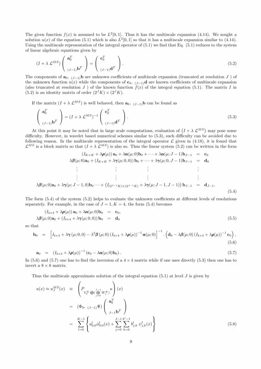
The given function f(x) is assumed to be L2[0, 1]. Thus it has the multiscale expansion (4.14). We sought asolution u(x) of the equation (5.1) which is also L2[0, 1] so that it has a multiscale expansion similar to (4.14).Using the multiscale representation of the integral operator of (5.1) we find that Eq. (5.1) reduces to the systemof linear algebraic equations given by

(I + λ LMS)

aT0

(J−1)bT

=

cT0

(J−1)dT

. (5.2)

The components of a0, (J−1)b are unknown coefficients of multiscale expansion (truncated at resolution J ) ofthe unknown function u(x) while the components of c0, (J−1)d are known coefficients of multiscale expansion(also truncated at resolution J ) of the known function f(x) of the integral equation (5.1). The matrix I in(5.2) is an identity matrix of order (2JK)× (2JK).

If the matrix (I + λ LMS) is well behaved, then a0, (J−1)b can be found as aT0

(J−1)bT

= (I + λ LMS)−1

cT0

(J−1)dT

. (5.3)

At this point it may be noted that in large scale computations, evaluation of(I + λ LMS

)may pose some

difficulty. However, in wavelet based numerical schemes similar to (5.3), such difficulty can be avoided due tofollowing reason. In the multiscale representation of the integral operator L given in (4.18), it is found thatLMS is a block matrix so that (I + λ LMS) is also so. Thus the linear system (5.2) can be written in the form

(IK×K + λρρρ(µ)) a0 + λααα(µ; 0)b0 + · · ·+ λααα(µ; J − 1)bJ−1 = c0

λβββ(µ; 0)a0 + (IK×K + λγγγ(µ; 0, 0)) b0 + · · ·+ λγγγ(µ; 0, J − 1)bJ−1 = d0

......

......

......

......

λβββ(µ; 0)a0 + λγγγ(µ; J − 1, 0)b0 · · ·+(I(2J−1K)×(2J−1K) + λγγγ(µ; J − 1, J − 1)

)bJ−1 = dJ−1.

(5.4)

The form (5.4) of the system (5.2) helps to evaluate the unknown coefficients at different levels of resolutionsseparately. For example, in the case of J = 1,K = 4, the form (5.4) becomes

(I4×4 + λρρρ(µ)) a0 + λααα(µ; 0)b0 = c0,

λβββ(µ; 0)a0 + (I4×4 + λγγγ(µ; 0, 0)) b0 = d0 (5.5)

so that

b0 =[I4×4 + λγγγ (µ; 0, 0)− λ2βββ (µ; 0) (I4×4 + λρρρ(µ))

−1ααα(µ; 0)

]−1

.(d0 − λβββ(µ; 0) (I4×4 + λρρρ(µ))

−1c0

),

(5.6)

a0 = (I4×4 + λρρρ(µ))−1

(c0 − λααα(µ; 0)b0) . (5.7)

In (5.6) and (5.7) one has to find the inversion of a 4× 4 matrix while if one uses directly (5.3) then one has toinvert a 8× 8 matrix.

Thus the multiscale approximate solution of the integral equation (5.1) at level J is given by

u(x) ≈ uMSJ (x) ≡

PV K0

⊕(J−1⊕j=0

WKj )u

(x)

= (Φ0, (J−1)Ψ)

aT0

J−1bT

=

K−1∑l=0

al0,0φl0,0(x) +

J−1∑j=0

2j−1∑k=0

blj,k ψlj,k(x)

(5.8)

9

where the coefficients al0,0, blj,k

(l = 0, 1, . . . . . .K − 1, k = 0, 1, . . . . . . 2j−1, j = 0, 1, . . . J − 1

)are obtained ei-

ther by using (5.3) or by solving the linear systems (5.4).

5.1 Behaviour of u(x) at x = k2j

To find the behaviour of u(x) at any point in [0, 1], we choose the dyadic interval Ij,k =[k2j ,

k+12j

]and assume

that

u(x) ≈ constant

(x− k

2j

)νfor x ∈ Ij,k. (5.9)

If the value of ν is an integer, then u(x) is well behaved in Ij,k, but if ν is otherwise then u(x) is nonsmooth inIj,k. Thus the behaviour at each point of [0, 1] can be found from the wavelet coefficient in the following way.The wavelet coefficients of u(x) are given by

blj,k =

∫ 1

0

u(x) ψlj,k(x)dx

=

∫ k+1

2j

k

2j

u(x) ψlj,k(x)dx

≈ constant 2j2

∫ k+1

2j

k

2j

(x− k

2j

)νψl(2jx− k)dx

≈ constant

2j(ν+ 12 )

∫ 1

0

tν ψl(t)dt

=c1

2j(ν+ 12 ), where c1 is a constant. (5.10)

Similarly

blj+1,2k =

∫ 1

0

u(x) ψlj+1,2k(x)dx

=

∫ k+12

2j

k

2j

u(x) ψlj+1,2k(x)dx

≈ constant 2j+12

∫ k+12

2j

k

2j

(x− k

2j

)νψl(2jx− 2k)dx

≈ constant

2(j+1)(ν+ 12 )

∫ 1

0

tν ψl(t)dt

=c1

2(j+1)(ν+ 12 ). (5.11)

Thus,

blj,kblj+1,2k

≈ 2ν+ 12

so that

νj,k ≈ −1

2+ log2

(blj,k

blj+1,2k

)(5.12)

where νj,k stands for the Holder exponent ν as we were considering the behaviour of u(x) in Ij,k. It may benoted that for a given j and k, l takes up the values l = 0, 1, . . ., K − 1. Thus we choose an estimate for νj,kin Ij,k as

νj,k ≈ −1

2+ log2

supl∈{0,1,··· ,K−1}

dlj,k

supl∈{0,1,··· ,K−1}

dlj+1,2k

. (5.13)

This result may be used in estimating error in multiscale approximation uMSJ of u(x) as discussed in the following

section.

10

6 Error estimation

In order to estimate the error in the multiscale approximation uJ(x) of u(x) satisfying the integral equation(5.1), we use the fact that the multiscale expansion of u(x) is

u(x) =

K−1∑l=0

al0,0φl0,0(x) +

∞∑j=0

2j−1∑k=0

blj,kψlj,k(x)

(6.1)

which can be recast into the form

u(x) = uMSJ (x) +

K−1∑l=0

∞∑j=J

2j−1∑k=0

blj,kψlj,k(x) (6.2)

where uMSJ (x) is given by (5.8). Hence if we write

u = uMSJ + δu (6.3)

where δu is the error in the multiscale approximation at resolution J , then

δu =

K−1∑l=0

∞∑j=J

2j−1∑k=0

blj,kψlj,k(x). (6.4)

Using orthonormality property of ψlj,k(x), we find

||δu||L2[0,1] =

K−1∑l=0

∞∑j=J

2j−1∑k=0

||blj,k||2 1

2

. (6.5)

If u ∈ Cν [0, 1], then the right side of (6.5) is always bounded(cf. Alpert et al. (1993)) and a bound is given by

1

2Jν2

22ν ν!supx∈[0,1]

|u[ν](x)| (6.6)

where [ν] is the integer part of ν. Thus

||δu||L2[0,1] ≤ A2−Jν = Ae−(ν ln2)J , (6.7)

where A =sup

x∈[0,1]|u[ν](x)|

22ν−1ν! so that as J increases, the error decreases exponentially.

7 Illustrative examples

The efficiency of the method discussed here is tested through some illustrative examples in this section.

Example 1. Consider the integral equation

a u(x)− b∫ 1

0

u(t)

|x− t|µdt = f(x), 0 < µ < 1, x ∈ [0, 1] (7.1)

where a, b are constants (are different from the coefficients appearing in the multiscale expansion uMSJ (x) in

(5.8)) and

f(x) = a xν − b[x1+ν−µ Γ (1− µ)

{Γ (µ− 1− ν)

Γ (−ν)+

Γ (1 + ν)

Γ (2 + ν − µ)

}−Γ (µ− 1− ν) 2F1 (µ, µ− 1− ν;µ− ν;x)] , ν > −1. (7.2)

When ν is an integer the term Γ(µ−1−ν)Γ(−ν) is absent. It has the exact solution

u(x) = xν . (7.3)

11

Use of the multiscale representation LMS for the integral operator in (7.1) and c0, (J−1)d associated with themultiscale representation of f(x) given by (7.2) in the linear system (5.4) produces a0, (J−1)b in the evaluationof uJ(x). Some representative values of the components of a0 associated with u4(x) for K = 4, ν = 0, 1, 2, 3 andarbitrary µ are given in Table 7.1. The values of components of b0 are found to be identically zero. The valuesof the components of bj (1 ≤ j ≤ 3) have been calculated separately and are also found to be zero. From thevalues of the components of a0 presented in Table 7.1 and vanishing of components of bj (0 ≤ j ≤ 3), it appearsthat in contrast to the method of Lakestani et al. [35] (involving expansion of the unknown function u(x) in thebasis of integrals of Legendre multiwavelets, cf. Table 7.1) the multiscale approximation u4(x) derived here inthe basis of Legendre multiwavelets directly recovers the exact solution u4(x) = xν (ν = 0, 1, 2, 3) for K = 4irrespective of µ involved in the kernel.

Table 7.1: Values of the components of a0 associated with u4(x) for K = 4, ν = 0, 1, 2, 3 and arbitrary µ.

ν a00,0 a10,0 a20,0 a30,00 1 0 0 0

1 12

12√

30 0

2 13

12√

31

6√

50

3 14

3√

320

14√

51

20√

7

We present in Table 7.2 the coefficients bj,k (j = 0, 1, 2, k = 0, 1, 2, ..., 2j − 1) of multiscale expansion u4(x)obtained by using (5.3) for f(x) given in (7.3) for ν = 4, µ = 1

2 . From the numerical values of blj,k (l =

0, 1, 2, 3; k = 0, 1, ..., 2j − 1; j = 0, 1, 2) presented in Table 7.2 it is obvious that the wavelet coefficients arenon-zero for all l, k, j (j ≤ 3). Their values are significant for l = 0 in each k for every resolution j. Wehave computed an estimate of exponent of x of u(x) at x = 0 by using wavelet coefficients into the formula(5.13) and found the value of ν close to 4. From the distribution of wavelet coefficients presented in Table 7.2it appears that this function u(x) varies smoothly throughout the domain [0, 1]. It is in agreement with thenature of variation of the wavelet coefficients corresponding to the exact solution u(x) = x4.

Table 7.2: The coefficients bj,k (j = 0, 1, 2, k = 0, 1, 2, ..., 2j − 1) obtained by using (5.3) f or f(x) given in (7.2) for ν = 4, µ = 12

j blj ,k l = 0 l = 1 l = 2 l = 3

0 k = 0 0.00475259 −6.5068 × 10−9 −2.77528 × 10−9 −1.61331 × 10−9

1 k = 0 0.000210045 −2.5619 × 10−9 −2.10167 × 10−8 −1.32539 × 10−8

k = 1 0.000210026 −2.65057 × 10−8 9.47444 × 10−9 −2.50116 × 10−8

2 k = 0 9.28785 × 10−6 −3.25296 × 10−9 1.54518 × 10−9 −2.7898 × 10−10

k = 1 9.29208 × 10−6 −1.14207 × 10−8 4.2062 × 10−9 9.55591 × 10−10

k = 2 9.26152 × 10−6 −3.9878 × 10−8 6.69711 × 10−9 1.74787 × 10−8

k = 3 9.26848 × 10−6 −3.52072 × 10−8 −1.72759 × 10−8 −2.88594 × 10−8

Example 2. To compare the efficiency of numerical method based on Legendre multiwavelets with otherschemes based on sinc collocation method of Okayama et-al [34], B-spline wavelet method of Maleknejad etal. [36], we consider the integral equation (5.1) with a = 1, b = 1

10 , µ = 13 and the input function

f(x) = x2(1− x)2 − 27

30800

{x

83

(54x2 − 126x+ 77

)+ (1− x)

83

(54x2 + 18x+ 5

)}. (7.4)

The exact solution for this equation is

u(x) = x2(1− x)2. (7.5)

We have used (7.4) in (5.6) for K = 4 and K = 5 and get all the wavelet coefficient to be zero in case of K = 5.The numerical values of u3(x) and u4(x) for x = i

10 (i = 0, 1, . . . , 10) obtained by the present method andmethods based on the aforesaid sinc collocation and B-spline wavelet are presented in Table 7.3. The results inthe Table 7.3 show that approximation of u(x)in the Legendre multiwavelets basis is more efficient than thoseobtained by sinc collocation method. The present method based on Legendre multiwavelets with K = 4 alsoproduces the same order of accuracy. It also produces the same results obtained by Maleknejad et al. [36] usingB-splines wavelet method.

12

Table 7.3: Exact and approximation value of u(x) in Ex.2, obtained by methods based on B-spline Wavelet (BSW), sinc collocation method

(SCM) and Legendre multiwavelets (LMW) basis.

x BSW SCM LMW K = 4 LMW K = 5 Exact

0 0 0 0 0 0

0.1 0.008103 0.00812 0.00810142 0.00810000 0.0081

0.2 0.025604 0.02565 0.0255992 0.02560000 0.0256

0.3 0.044101 0.04414 0.0440992 0.04410000 0.0441

0.4 0.057609 0.05768 0.0576014 0.05760000 0.0576

0.5 0.062503 0.06259 0.0624965 0.06250000 0.0625

0.6 0.057608 0.05763 0.0576014 0.05760000 0.0576

0.7 0.044102 0.04414 0.0440992 0.04410000 0.0441

0.8 0.025606 0.02563 0.0255992 0.02560000 0.0256

0.9 0.008104 0.00816 0.00810142 0.00810000 0.0081

1 0 0 0 0 0

Example 3. Here we consider the integral equation (7.1) [13, 34, 36] with a = 3√

24 , b = 1, µ = 1

2 and theforcing term as

f(x) = 3 {x (1− x)}34 − 3π

8{1 + 4x (1− x)} . (7.6)

It has the exact solution u(x) = 2√

2 {x(1− x)}34 . Here f(x) is continuous but not differentiable at the end

points x = 0 and x = 1.

The components blj,k (k = 0, 1, ..., 2j − 1) involved in the multiscale expansion u4(x) of the solution u(x) ofthis integral equation are presented in Table 7.4.

Table 7.4: The components blj,k (j = 0, 1, 2; k = 0, 1, ..., 2j − 1) involved in the multiscale expansion corresponding to the input function

(7.6)

j blj ,k l = 0 l = 1 l = 2 l = 3

0 k = 0 −0.0204132 −8.44085 × 10−8 −0.00340831 −2.23761 × 10−7

1 k = 0 −0.00408052 0.0018308 −0.000695451 0.000162144

k = 1 −0.00408034 −0.00183057 −0.000696108 −0.000161366

2 k = 0 −0.00164317 0.000758449 −0.000290236 6.20468 × 10−5

k = 1 −2.09343 × 10−5 2.05699 × 10−6 −1.93802 × 10−7 −2.90463 × 10−7

k = 2 −2.88933 × 10−5 4.44472 × 10−6 −2.68388 × 10−6 1.17356 × 10−7

k = 3 −0.00164308 −0.000758193 −0.000290211 −6.20326 × 10−5

Table 7.5: Estimation of Holder exponent of u(x) around the end points

j νj ,0 νj,2j−1

0 1.8 1.8

1 .87 .87

2 .76 .76

From the values of the wavelet coefficients presented in Table 7.4 it is obvious that the solution possessesrapid variation around the end points x = 0 and x = 1 due to relatively large values of wavelet coefficients fork = 0 and k = 2j − 1 for each j. In order to estimate Holder exponent of u(x) around the end points we usethe results of Table 7.4 into formula (5.13). The estimated values of νj,0 and νj,2j−1 are presented in Table 7.5for j = 0, 1, 2. The sequences {νj,0, j = 0, 1, 2} and {νj,2j−1, j = 0, 1, 2} are found to be rapidly convergentand converge to the exact value ν = .75. The approximate solution u3(x) and the absolute error of the solutionare presented in Fig 7.1a and Fig 7.1b respectively. We have used the formula (6.5) to estimate || ||L2 error byusing values of coefficients presented in Table 7.4 and found it to be .001. This estimate is in good agreementwith the absolute error presented in Fig 7.1b in most of the region 0 < x < 1. The accuracy can be improvedfurther by increasing the resolution j appropriately.

In order to compare the efficiency of estimate of ||u(x) − uMSJ ||L2[0,1] by its norm equivalence presented in

(6.5), we have evaluated the L2-error√∫ 1

0{u(x)− uMS

J (x)}2dx and the RHS of (6.5) for all three examples

discussed here. Those results have presented in Table 7.6 and found to be equal up to two significant digits.

8 Conclusion

The purpose of this work is to develop a multiscale approximation scheme based on Legendre multiwavelets forsolving Fredholm integral equation of second kind with weakly singular kernel. In the process of our development

13

Table 7.6: The L2 error ||u(x)− uMSJ ||L2[0,1] and its equivalence formula (6.5) for all examples

Formula Ex-1 Ex-2 Ex-3

||u(x) − uMS3 ||L2[0,1]

1.2 × 10−6 1.2 × 10−6 1.0 × 10−3

RHS of (6.5) 1.24 × 10−6 1.24 × 10−6 1.0 × 10−3

the low- and high-pass filters for two-scale relations involving Legendre multiwavelets having 4 or 5 componentsat scale j = 0 have been evaluated and the recurrence relations amongst elements or formulas involving theelements of the multiscale representation of the integral operator have been derived. Analytical expressions forsome important matrix elements (ρρρ) in terms of µ (appears as exponent in the singular kernel) are presented herefor their use in the formulas derived in section 3.2 and section 3.3 for evaluation of other matrix elements (viz.α, β, γα, β, γα, β, γ) of LMS . We have derived here a formula for the estimation of the Holder exponent of the unknownsolution of the integral equation at any point within its domain and is used to estimate error in multiscaleapproximation of the solution. The error in approximation scheme studied here is found to be of exponentialorder.

The efficiency of the method has been tested by comparing results obtained by the present method and othermethods for a few examples. From our study it appears that the efficiency of the multiscale approximation ofsolution of a Fredholm integral equation of second kind with weakly singular kernel in the direct Legendre mul-tiwavelet basis is better than their expansion in the basis of integrals of Legendre multiwavelets as used in [35].Note that the numerical scheme developed here is limited to the Fredholm integral equation of second kindwith constant coefficients in one dimension. Its performance in comparison to existing approximation schemesmotivates us to extend it to get multiscale approximation and local behaviour of solution of integro-differentialequations, integro-differential difference equations with constant or variable coefficients, integral equations in-volving regular or nonsmooth input functions with weakly-,Cauchy- or hypersingular kernel in one or higherdimensions. Works in these directions are in progress and will be reported in due course.

(a) (b)Fig.7.1: a) Approximate solution u3(x) b) Absolute error

AcknowledgementsThis work is supported by a research grant from SERB(DST), No. SR/S4/MS:821/13.

References

[1] J. C. Nedelec, Acoustic and Electromagnetic Equations: Integral Representations for Harmonic Problems,

Springer, NY 2001.

[2] R. Pike, P. Sabatier, Scattering : Scattering and Inverse Scattering in Pure and Applied Science, Academic

Press, San Diego, 2002.

[3] D. Colton, R. Kress, Inverse Accoustic and Electromagnetic Scattering Theory, Springer (3rd Ed.), NY.

2013.

[4] N. I. Muskhelishvilli, Singular Integral Equations, Nordhoft, Groningen, 1953.

14

[5] S. Mikhlin, S. Prossderf, Singular Integral Operators, Academic-Verlag, Berlin 1986.

[6] R. P. Kanwal, Linear Integral Equations, Birkhauser Verlag, Baston 1996.

[7] K. Atkinson, W. Han, Theoretical Numerical Analysis : A Functional Analysis Framework, (3rd Ed.), Text

in Applied Mathematics, Springer 2009.

[8] K. E. Atkinson, The Numerical Solution of Integral Equations of the Second Kind, Cambridge University

Press, Cambridge, 1997.

[9] A. Pedas, G. Vainikko, Smoothing transformation and piecewise polynomial projection methods for weakly

singular Fredholm integral equations, Commun. Pure Appl. Anal. 5 (2006) 395-413.

[10] Y. Cao, M. Huang, L. Liu, Y. Xuc, Hybrid collocation methods for Fredholm integral equations with weakly

singuar kernels, Appl. Numer. Math. 57 (2007) 549-561.

[11] T. Diago, S. Mckee, T. Tang, A Hermite-type collocation method for the solution of an integral equation

with a certain weakly singular kernel, IMA J. Numer. Anal. 11 (1991) 595-605.

[12] R. Pallav, A. Pedas, Quadratic spline collocation method for weakly singular integral equations and corre-

sponding eigenvalue problem, Math Model. Anal. 7 (2002) 285-296.

[13] C. Schneider, Product integration for weakly singular integral equations, Math. Comput. 36 (1981) 207-213.

[14] P. Assari, H. Adidbi, M. Dehghan, The numerical solution of weakly singular integral equations based on

the meshless product integration (MPI) method with error analysis, Appl. Numer. Math. 81 (2014) 76-93.

[15] P. Assari, H. Adidbi, M. Dehghan, A meshless discrete Galerkin (MDG) method for the numerical solution

of integral equations with logarithimic kernels, J. Comp. Appl. Math. 267 (2014) 160-181.

[16] M. Dehghan, R. Salehi, The numerical solution of the non-linear integro-differential equations based on the

meshless method, J. Comp. Appl. Math. 236 (2012) 2367-2377.

[17] D. Mirzaei, M. Dehghan, A meshless based method for solution of integral equations, Appl. Numer. Math.

60 (2010) 245-262.

[18] M. Dehghan, Solution of a partial integro-differential equation arising from viscoelasticity, Intern. J. Comp.

Math. 83 (2006) 123-129.

[19] SA. Yousefi, A. Lotfi, M. Dehghan, The use of a Legendre multiwavelet collocation method for solving the

fractional optimal control problems, J. Vibration and Control 17(13) (2011) 2059-2065.

[20] B. K. Alpert, A class of bases in L2 for the sparse representation of integral operators, SIAM J. Math.

Anal. 24 (1993) 246-262.

[21] B. K. Alpert, G. Beylkin, R. Coifman, V. Rokhlin, Wavelet-like bases for the fast solution of second-kind

integral equations, SIAM J. Sci. Comput. 14 (1993) 159-184.

[22] Y. Cao, Y. Xu, Singularity preserving Galerkin methods for weakly singular Fredholm integral equations,

J. Int. Equations Appl. 6 (1994) 303-334.

[23] C. A. Micchelli, Y. Xu, Y. Zhao, Wavelet-Galerkian methods for second kind integral equations, J. Comput.

Appl. Math. 86 (1997) 251-270.

[24] Z. Chen, C. A. Micchelli, Y. Xu, The Petrov-Galerkian method for second kind integral equations II:

Multiwavelet scheme, Adv. Comput. Math. 7 (1997) 199-233.

15

[25] T. V. Petersdroff, C. Schwab, R. Schneider, Multiwavelets for second-kind integral equations, SIAM J.

Numer. Anal. 34 (1997) 2212-2227.

[26] Z. Chen, Y. Xu, The Petrov-Galerkian and iterated Petrov-Galerkian methods for second kind integral

equations, SIAM J. Numer. Anal. 35 (1998) 406-434.

[27] Z. Chen, C. A. Micchelli, Y. Xu, Fast collocation methods for second kind integral equations, SIAM J.

Numer. Anal. 40 (2002) 344-375.

[28] I. Daubechies, Ten Lectures on Wavelets, CBMS Lecture notes, SIAM publication, 1992.

[29] Y. Meyer, Wavelets and Operators, Cambridge University Press, Cambridge 1992.

[30] Y. Meyer, R. Coifman, Wavelets: Calderon-Zygmund and Multilinear Operator, Cambridge University

Press, 1997.

[31] A. Cohen, Numerical Analysis of Wavelet Methods, Elsevier, Amsterdam 2003.

[32] G. W. Pan, Wavelets in Electromagnetics and Device Modeling, Wiley-Interscience, 2003.

[33] M. Huang, A construction of multiscale bases for Petrov-Galerkin methods for integral equations, Adv.

Comput. Math. 25 (2006) 7-22.

[34] T. Okayama, T. Matsuo, M. Sugihara, Sinc-collocation methods for weakly singular Fredholm integral

equations of the second kind, J. Comp. Appl. Math. 234 (2010) 1211-1227.

[35] M. Lakestani, B. N. Saray, M. Dehghan, Numerical solution for the weakly singular Fredholm integro-

differential equations using Legendre multiwavelets, J. Comput. Appl. Math. 235 (2011) 3291-3303.

[36] K. Maleknejad, M. Nosrati, E. Najati, Wavelet Galerkian method for solving singular integral equations,

Comp. Appl. Math. 31 (2012) 373-390.

[37] H. T. Cai, A Jacobi-collocation method for solving second kind Fredholm integral equations with weakly

singular kernels, Sci China Math 57 (2014) doi:10.1007/S11425-014-4806-2.

[38] B. K. Alpert, G. Beylkin, D. Gines, L. Vozovoi, Adaptive solution of partial differential equations in

multiwavelet bases, J. Comput. Phys. 182 (2002) 149-190.

16