No. 2003–122

MULTIVARIATE OPTION PRICING USING DYNAMIC COPULA MODELS

By R.W.J. van den Goorbergh, C. Genest, B.J.M. Werker

December 2003

ISSN 0924-7815

Multivariate Option Pricing Using

Dynamic Copula Models

Rob W. J. van den Goorbergh∗ Christian Genest†

Bas J. M. Werker‡

This version: September 30, 2003

Abstract

This paper examines the behavior of multivariate option prices in thepresence of association between the underlying assets. Parametric fam-ilies of copulas offering various alternatives to the normal dependencestructure are used to model this association, which is explicitly as-sumed to vary over time as a function of the volatilities of the assets.These dynamic copula models are applied to better-of-two-markets andworse-of-two-markets options on the S&P500 and Nasdaq indexes. Re-sults show that option prices implied by dynamic copula models differsubstantially from prices implied by models that fix the dependencebetween the underlyings, particularly in times of high volatilities. Fur-thermore, the normal copula produces option prices that differ signif-icantly from non-normal copula prices, irrespective of initial volatilitylevels. Within the class of non-normal copula families considered, op-tion prices are robust with respect to the copula choice.

JEL classification: G13.Keywords: Time-varying dependence, best-of-two-markets options, non-normality.

∗Department of Finance and CentER for Economic Research, Tilburg University,PO Box 90153, 5000 LE Tilburg, The Netherlands. Corresponding author. E-mail:r.w.j.vdngoorbergh@uvt.nl, Phone: +31 (0)13 466 8222, Fax: +31 (0)13 466 2875.

†Departement de mathematiques et de statistique, Universite Laval, Quebec, CanadaG1K 7P4.

‡Department of Finance, Department of Econometrics and Operations Research, andCentER for Economic Research, Tilburg University, Tilburg, The Netherlands.

1

1 Introduction

In today’s economy, multivariate (or rainbow) options are viewed as excellenttools for hedging the risk of multiple assets. These options, which are writtenon two or more underlying securities or indexes, usually take the form of calls(or puts) that give the right to buy (or sell) the best or worst performer ofa number of underlying assets. Other examples include forward contractswhose payoff is equal to that of the best or worst performer of its underlyings,and spread options on the difference between the prices of two assets.

One of the key determinants in the valuation of multivariate optionsis the dependence between the underlying assets. Consider for instance abivariate call-on-max option, namely a contract that gives the holder theright to purchase the more valuable of two underlying assets for a pre-specified strike price. Intuitively, the value of such an option should besmaller if the underlyings tend to move together than when they move inopposite directions. More generally, the dependence between the underlyingscould change over time. Accounting for time variation in the dependencestructure between assets should prove helpful in providing a more realisticvaluation of multivariate options.

Over the years, various generalizations of the Black–Scholes (1973) Brow-nian motion framework have been used to model multivariate option prices.Examples include Margrabe (1978), Stulz (1982), Johnson (1987), Reiner(1992), and Shimko (1994). In these papers, the dependence between as-sets is modelled by their correlation. However, unless asset returns are wellrepresented by a multivariate normal distribution, correlation is often anunsatisfactory measure of dependence; see, for instance, Embrechts, Mc-Neil, and Straumann (2002). Furthermore, it is a stylized fact of financialmarkets that correlations observed under ordinary market conditions differsubstantially from correlations observed in hectic periods. In particular,asset prices have a greater tendency to move together in bad states of theeconomy than in quiet periods; see, for instance, Boyer, Gibson, and Loretan(1999) and Patton (2002a, 2002b) and references therein. These “correla-tion breakdowns,” associated with economic downturns, suggest a dynamicmodel of the dependence structure of asset returns.

In this paper, the relation between multivariate option prices and thedependence structure of the underlying financial assets is modelled dynami-cally through copulas. A copula is a multivariate distribution function eachof whose marginals is uniform on the unit interval. It has been known sincethe work of Sklar (1959) that any multivariate continuous distribution func-tion can be uniquely factored into its marginals and a copula. Thus while

2

correlation measures dependence through a single number, the dependencebetween multiple assets is fully captured by the copula. From a practicalpoint of view, the advantage of the copula-based approach to modelling isthat appropriate marginal distributions for the components of a multivari-ate system can be selected by any desired method, and then linked througha copula or family of copulas suitably chosen to represent the dependenceprevailing between the components.

The use of copulas to price multivariate options is not new. For example,in Rosenberg (1999), univariate options data are used to estimate marginalrisk-neutral densities, which are linked with a Plackett copula to obtain abivariate risk-neutral density from which bivariate claims are valuated. Thissemiparametric procedure uses a particular identifying assumption on therisk-neutral correlation to fix the copula parameter. Cherubini and Luciano(2002) extend Rosenberg’s work by considering other families of copulas.In Rosenberg (2003), a risk-neutral bivariate distribution is estimated fromnonparametric estimates of the marginal distributions and a nonparametricestimate of the copula.

An innovating feature of the present paper, however, is that, contraryto earlier works on multivariate option pricing, the dependence structure ofthe underlying assets is not treated as fixed, but rather as possibly varyingover time. Taking into account this time variation is important because itmay influence option prices. This paper proposes a model for the time vari-ation of the dependence structure, in which a parametric copula is specifiedwhose dependence parameter is allowed to change with the volatilities ofthe underlying assets. A distinct advantage of the parametric approach isthat while the model may be misspecified, the robustness of the conclusionscan easily be verified by repeating the analysis for as many different copulafamilies as desired.

A similar dynamic-copula approach has already been used in the foreignexchange market literature by Patton (2002a), who found time variationto be significant in a copula model for asymmetric dependence betweentwo exchange rates where the dependence parameter followed a ARMA-type process. While Patton’s goal was to study the effect of asymmetricdependence on portfolio returns, the objective of the present paper is verydifferent. The main focus here is on the effect of time variation in theunderlying dependence structure on the price of multivariate options.

In the empirical study presented herein, multivariate options on two im-portant American equity index returns are considered: the S&P500 and theNasdaq. An analysis of the results suggests that allowing for time variationin the dependence structure of the underlyings produces substantially dif-

3

ferent option prices than under constant dependence, particularly in timesof increased volatility. Moreover, option prices implied by a normal dy-namic dependence structure differ significantly from option prices impliedby non-normal dynamic dependence structures. These findings suggest thatunless the dependence between the S&P500 and Nasdaq stock indexes is welldescribed by a normal copula, alternative copula families should be consid-ered. Option prices turned out to be robust among the alternative—i.e.,non-normal—copula models considered in this study.

The remainder of this paper is organized as follows. Section 2 describesthe payoff structure of better-of-two-markets and worse-of-two-marketsclaims, and explains in detail the proposed dynamic-dependence option val-uation scheme. The empirical results are presented in Section 3, and con-clusions are given in Section 4.

2 Option valuation with time-varying dependence

Multivariate options come in a wide variety of payoff schemes. The mostcommonly traded options of this kind are basket options on a portfolio ofassets, such as index options. Other examples include spread options, someof which are traded on commodity exchanges (see, for example, Rosenberg(1998)), or dual-strike and multivariate-digital options.

This paper concentrates on European-type options on the best (worst)performer of several assets, sometimes referred to as outperformance (un-derperformance) options. As these are typically traded over the counter,price data are not available. Therefore, valuation models cannot be testedempirically. However, a robustness study comparing models with differ-ent assumptions remains feasible, and this is the objective pursued herein.While the study described in the sequel is restricted to options on better-and worse-of-two-markets claims, the technique is sufficiently general to an-alyze the aforementioned alternative multivariate options as well, and maythus be of wider interest.

One can distinguish four types of better-of-two-markets or worse-of-two-markets claims: call options on the better performer, put options on theworse performer, call options on the worse performer, and put options onthe better performer. These may be referred to as call-on-max, put-on-min,call-on-min, and put-on-max options, respectively. Their payoffs at maturityare:

4

call on max : max{max(R1, R2)−E, 0},put on min : max{E −min(R1, R2), 0},call on min : max{min(R1, R2)−E, 0},put on max : max{E −max(R1, R2), 0},

where Ri is the return at maturity on index i ∈ {1, 2}, and E denotes theexercise price of the option.

The proposed scheme for valuating these options is as follows. First,each of the two objective marginal distributions of the daily index returnsunderlying a type of claim is modelled, and their risk-neutral counterpartsare derived. Next, a parametric family of copulas is chosen to fix the jointrisk-neutral distribution of the index returns. The fair value of the optionis then determined by taking the discounted expected value of the option’spayoff under the risk-neutral distribution.

The specification chosen for the objective marginal distributions is fromDuan (1995). It is general enough to capture volatility clustering, a stylizedfact of equity returns for which there is overwhelming empirical evidence atthe daily frequency, while still providing a relatively easy transformation torisk-neutral distributions. Each of the objective marginal distributions ofthe index returns is modelled by a GARCH(1,1) process. It is repeated herefor the sake of completeness; see Bollerslev (1986). For i ∈ {1, 2},

Ri,t+1 = µi + ηi,t+1 ,

ηi,t+1|It ∼ N (0, hi,t) ,

hi,t+1 = ωi + βihi,t + αiη2i,t+1,

where ωi > 0, βi > 0, and αi > 0. Here, It denotes the informationavailable at time t. However, it must be stressed that, in the light of Sklar’stheorem, in principle any choice for the marginal distributions is consistentwith the copula approach. The vast collection of alternatives that havebeen used by other authors to model univariate index return distributionsincludes (variants of) continuous-time geometric Brownian motion of Blackand Scholes (1973), and the discrete-time binomial model of Cox, Ross, andRubinstein (1979). Again, the GARCH specification that is employed hereis appealing as it allows for an easy change of measure in addition to beingable to capture volatility clustering. In particular, Duan (1995) shows that,under certain conditions, the change of measure comes down to a change inthe drift.

An alternative, nonparametric approach is to use univariate option pricedata to obtain arbitrage-free estimates of the marginal risk-neutral densities,

5

as in Ait-Sahalia and Lo (1998). This route is taken by Rosenberg (2003).Clearly, an advantage of this approach is that it does not impose restrictionson the asset return processes or on the functional form of the risk-neutraldensities. However, this flexibility comes at the cost of imprecise estimates,especially if the distributions are time-varying.

The second step in the proposed valuation scheme is to fix the jointrisk-neutral distribution of the index returns by choosing a copula. A setof well-known one-parameter copula families is considered for this purpose.They are the Frank, Gumbel–Hougaard, Plackett, Galambos, and normalfamilies. Their cumulative distribution functions are given in Appendix A.For all of these copulas, there is a one-to-one relation between the depen-dence parameter—denoted θ—and Kendall’s nonparametric measure of as-sociation. For any copula Cθ, Kendall’s tau is related to θ in the followingway:

τ(θ) = 4ECθ(U, V )− 1, (1)

where (U, V ) is distributed as Cθ, and E denotes the expectation operatorwith respect to U and V . Appendix B displays closed-form formulas forthe population value of Kendall’s tau for some of the copula models underconsideration.

This relation suggests a natural way to estimate the copula. An esti-mate of θ is readily obtained by computing the sample version of tau ona (sub)sample of paired index-return observations, inverting Relation (1),and plugging in the sample tau.1 This method-of-moment type procedureyields a rank-based estimate of the association parameter which is consis-tent, under the assumption that the selected family of copulas describesaccurately the dependence structure of the equity indexes. Other methodscould be used without fundamentally altering this approach, e.g., inversionof Spearman’s rho, or the maximum pseudo-likelihood method.

The proposed technique assumes that the objective and risk-neutralcopulas are identical. Rosenberg (2003) makes this assumption as well.If multivariate option price data were available, this assumption could betested or the appropriate risk-neutral copula could be estimated. Only dataon prices of multivariate claims would reveal information about the risk-neutral dependence structure. Information about the risk-neutral depen-

1The sample version of Kendall’s tau is defined as follows. Let {(X1, Y1), . . . , (Xn, Yn)}be a random sample of n observations from a vector (X, Y ) of continuous random variables.Two distinct pairs (Xi, Yi) and (Xj , Yj) are said to be concordant if (Xi−Xj)(Yi−Yj) > 0,and discordant if (Xi −Xj)(Yi − Yj) < 0. Kendall’s tau for the sample is then defined ast = (c− d)/(c + d), where c denotes the number of concordant pairs, and d is the numberof discordant pairs.

6

dence structure can never be extracted from univariate option prices—whichare available—as these only bear relevance to the risk-neutral marginal pro-cesses, and not to the joint risk-neutral process. Identification of the mul-tivariate density requires knowledge of both the marginal densities and thedependence function that links them together.

Time variation in the copula is modelled by allowing the parameter ofdependence parameter to evolve through time according to a particular equa-tion. The forcing variables in this equation are the conditional volatilities ofthe underlying assets. These are also the forcing variables that are typicallychosen to model time-varying correlations; see, e.g., the BEKK model intro-duced by Engle and Kroner (1995). Additional motivation is provided bythe evidence on correlation breakdowns, which suggests that financial mar-kets exhibit high dependence in periods of high volatility. Patton (2002a)proposes an ARMA-type process linking the dependence parameter to ab-solute differences in return innovations, which is another way to capture thesame idea.

To be more specific, let τt be Kendall’s measure of association at timet, and let hi,t be the objective conditional variance estimate at time t ofunderlying index return i ∈ {1, 2} implied by Duan’s GARCH option pricingmodel. It is assumed that

τt = γ(h1,t, h2,t) (2)

for some function γ(·, ·) to be specified later. This conditional measure ofassociation governs the degree of dependence for the risk-neutral copulaunder consideration.

The proposed valuation scheme is implemented using Monte Carlo simu-lations. Pairs of random variates are drawn from the copula implied by theestimated conditional risk-neutral measure of association, which are thentransformed to return innovations using Duan’s GARCH model. Subse-quently, the payoffs implied by these innovations are averaged and dis-counted at the risk-free rate. The result then constitutes the fair valueof the option. Algorithms for random variable generation from the non-normal copulas are given in Genest and MacKay (1986), Genest (1987),Ghoudi, Khoudraji, and Rivest (1998), and Nelsen (1999). For the normalcopula, a straightforward Cholesky decomposition may be used.

7

3 Pricing options on two equity indexes

The dynamic-dependence valuation scheme outlined in Section 2 is appliedto better-of-two-markets and worse-of-two-markets options on the S&P500and Nasdaq indexes. A sample consisting of pairs of daily returns on theS&P500 and Nasdaq from January 1, 1993 to August 30, 2002 was obtainedfrom Datastream. The sample size is T = 2422. The maximum likelihoodestimates of the GARCH parameters for the marginal index return processesmay be found in Table I. The values for α and β nearly add up to one. Theseestimates are in line with previously reported values.

Figure 1 depicts the time series of the estimated standardized GARCHinnovations (η1,t+1/

√h1,t, η2,t+1/

√h2,t) for the last 250 trading days in the

sample. (For clarity, the picture is restricted to a subsample; other episodesshow a similar pattern.) Note that outliers typically occur simultaneouslyand in the same direction. This positive dependence between the two se-ries is even more apparent from Figure 2, which displays the support setof the empirical copula of the standardized return innovations. This scat-ter plot consists of the observed pairs of ranks (divided by T + 1) for theestimated standardized GARCH innovations of the two markets. Under reg-ularity conditions, the empirical copula function converges to the true (here,objective) copula function; see Van der Vaart and Wellner (1996). Noticethe pronounced positive dependence, particularly in the tails. The sampleversion of Kendall’s tau for the entire sample amounts to 0.60, confirmingpositive dependence. Figure 3 gives an impression of how this dependencemeasure of the standardized return innovations evolves over time. It showsrolling-window estimates of Kendall’s tau using window sizes of two months,i.e., Kendall’s tau at day t is computed using the 20 trading days prior today t, day t itself, and the 20 trading days after day t. While the estimatesshow considerable variation, a slightly upward trend over the sample periodis discernable.

The time variation in the copula is governed by Equation (2). It modelsthe dependence measure as a function of the conditional volatilities of theindex returns. The following specification of this function is proposed:

γ(h1, h2) = γ0 + γ1 log max(h1, h2). (3)

To motivate this specification, recall that the evidence on correlation break-downs suggests that increased dependence occurs in hectic periods. Hence,theory predicts a positive value of γ1. The maximum operator reflects thathectic periods in either market may cause dependence to go up. Since volatil-ity in both markets is highly dependent, the actual specification is likely not

8

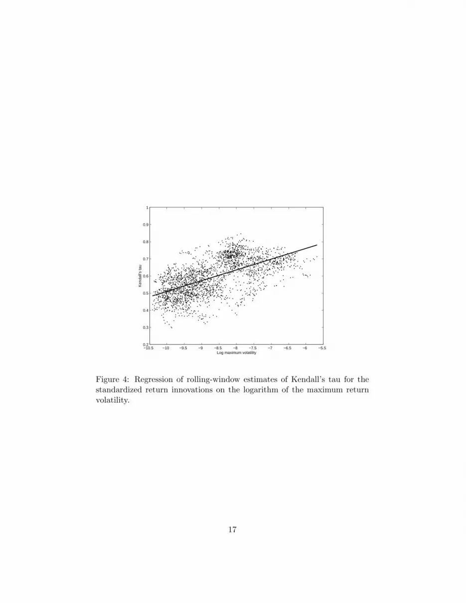
to affect the results in the present section too much. The parameters γ0 andγ1 were estimated by regressing the rolling-window estimates of Kendall’stau on the estimated log maximum conditional volatility. This is illustratedin Figure 4. The slope coefficient, γ1, was estimated at 0.063; positive, asexpected. The estimated dependence measure implied by these parameterestimates,

γ(h1,t, h2,t) = γ0 + γ1 log max(h1,t, h2,t),

was then used to fix the conditional risk-neutral copula at time t. Returninnovations were sampled from this conditional copula to compute the priceof the option. In total, the Monte Carlo study was based on 100, 000 repli-cations, leading to simulation errors in the order of magnitude of 1 basispoint for one-month maturity claims.

Clearly, the option price depends on the initial levels of volatility ofthe underlyings. Prices for three levels of initial volatility were computed:low, medium, and high volatility, where medium volatility is defined as theestimated unconditional variance ω/(1−β−α), and low and high volatilityare one-fourth of and four times this amount, respectively. Furthermore,different maturities were considered, ranging from one day to one month(i.e., 20 trading days). The strike price was set at levels between .98 and1.02. Finally, the risk-free rate was assumed to be 4 percent per annum.

The results show that allowing for time varying dependence leads todifferent option prices than under static dependence, in particular in timesof high volatility. This is illustrated in Figure 5 which displays, for variouscopula parametrizations, the price (measured in basis points) of a one-monthput-on-max option as a function of the exercise price implied by dynamicdependence, and compares it to the option price under three levels of staticdependence: low, medium, and high static dependence. The medium levelof dependence is equal to the average measure of dependence found in thesample, 0.60; the low and high levels are 0.40 and 0.80, respectively. Notethat a static model for the dependence structure, which uses the samplemeasure of dependence of 0.60, underestimates the option price generated bythe dynamic model considerably for all copula parametrizations and over theentire range of strike prices considered. The difference is significant since the95% confidence intervals of the price estimates do not overlap. In the interestof clarity, confidence intervals are not displayed here, but available from theauthors upon request. Note that the prices implied by dynamic copulas arebetween the high and the medium static-dependence prices, suggesting thatthe dynamic model implies a dependence that is on average stronger than inthe medium static-dependence case. Interestingly, price differences between

9

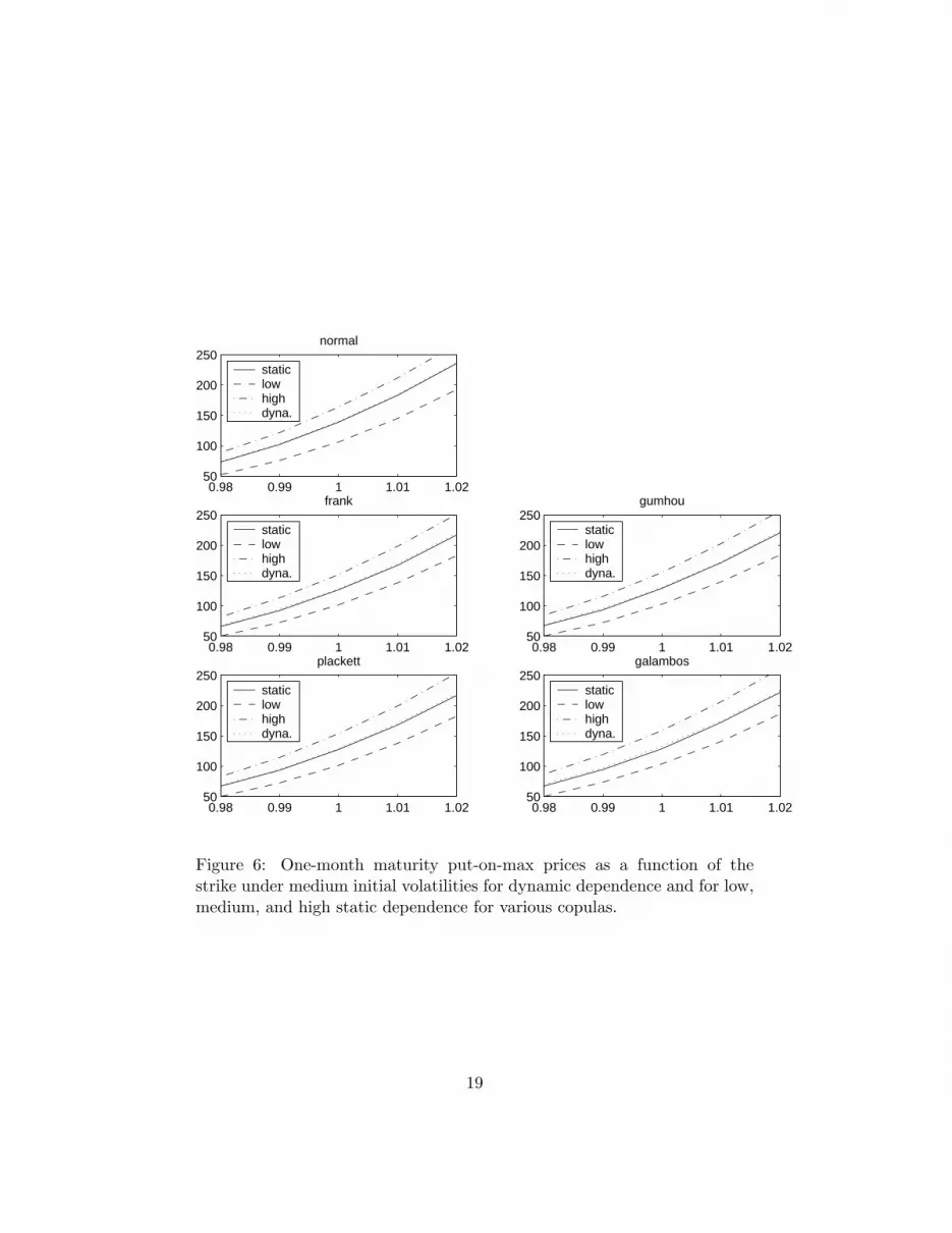
the dynamic and static model vanish as initial volatilities are at a mediumlevel; see Figure 6. The same holds for low initial volatilities (not shown),again, across a broad range of copula families and strike prices.

It is also interesting to compare option prices produced by different dy-namic copula families. It turns out that prices implied by the normal cop-ula deviate substantially from prices implied by the other copula families.Outside the normal class, the copula choice appears to be irrelevant. Thissuggests that unless the dependence between index returns can be describedby a normal model, alternative specifications should be considered. Thesefindings are illustrated in Figures 7 and 8 which depict dynamic-dependenceone-month call-on-max and put-on-min option prices respectively, as a func-tion of their strike under medium initial volatilities. The prices implied bythe normal copula are significantly lower than the prices implied by the othercopulas across the whole range of strike prices. The effect is there at othermaturities as well. The difference between normal and non-normal prices isalso found for high and low initial volatility levels. The differences are lesssignificant for call-on-min and put-on-max options.

4 Conclusions

This paper studies the relation between multivariate options prices and thedependence structure of the underlying assets. A copula-based model wasproposed for the valuation of claims on multiple assets. A novel feature ofthe proposed model is that, contrary to earlier works on multivariate optionpricing, the dependence structure is not taken as fixed, but rather as poten-tially varying with time. The time variation in the dependence structure wasmodelled using various parametric copulas by letting the copula parameterdepend on the conditional volatilities of the underlyings.

This dynamic copula model was applied to better- and worse-of-two-markets options on the S&P500 and Nasdaq indexes for a variety of copulaparametrizations. Option prices implied by the dynamic model turned outto differ substantially from prices implied by a model that fixes the depen-dence between the underlying indexes, especially in high-volatility marketconditions. Hence, the application suggests that time variation in the de-pendence between the S&P500 and the Nasdaq is important for the priceof options on these indexes. A comparison of option prices computed fromdifferent copula families shows that the normal family produces prices thatdiffer significantly from the ones implied by the non-normal alternatives.These findings suggests that if the dependence between the index returns

10

is not well represented by a normal copula, alternative copulas need to beconsidered. The empirical relevance of such alternatives is apparent giventhe evidence of non-normality in financial markets.

11

A One-Parameter Copula Families

The table below displays several one-parameter copula families.

Frank Cθ(u, v) = 1θ log

{1 + (eθu−1)(eθv−1)

eθ−1

}

Gumbel–Hougaard Cθ(u, v) = exp{−

(| log u|θ + | log v|θ

) 1θ

}

Plackett Cθ(u, v) = 1+(θ−1)(u+v)−√

[1+(θ−1)(u+v)]2−4uvθ(θ−1)

2(θ−1)

Galambos Cθ(u, v) = uv exp{(| log u|θ + | log v|θ

)− 1θ

}

Normal Cθ(u, v) = Nθ(Φ−1(u),Φ−1(v))

Note: Φ is the standard (univariate) normal distribution function, and Nθ denotes the

standard bivariate normal distribution function with correlation coefficient θ.

B Kendall’s tau

The table below provides expressions—closed-form if available—of the re-lation between Kendall’s tau and the dependence parameter for the copulafamilies considered in Appendix A.

Frank τ(θ) = 1− 4 {D1(−θ)− 1} /θ

Gumbel-Hougaard τ(θ) = 1− 1/θ

Plackett τ(θ) = 4∫ 10

∫ 10 Cθ(u, v)dCθ(u, v)− 1

Galambos τ(θ) = θ+1θ

∫ 10

(1

t1/θ + 1(1−t)1/θ − 1

)−1dt

Normal τ(θ) = 2π arcsin θ

Note: D1 denote the first-order Debye function, D1(−θ) = 1θ

∫ θ

0t

et−1dt + θ

2.

12

References

Ait-Sahalia, Yacine, and Andrew W. Lo, 1998, Nonparametric Estimationof State-Price Densities Implicit in Financial Asset Prices, Journal ofFinance 53, 499–547.

Black, Fisher, and Myron S. Scholes, 1973, The Pricing of Options andCorporate Liabilities, Journal of Political Economy 81, 637–654.

Bollerslev, Tim, 1986, Generalized Autoregressive Conditional Het-eroskedasticity, Journal of Econometrics 31, 307–327.

Boyer, Brian H., Michael S. Gibson, and Mico Loretan, 1999, Pitfalls inTests for Changes in Correlations, Working paper, International FinanceDiscussion Papers, No. 597, Board of Governors of the Federal ReserveSystem.

Cherubini, Umberto, and Elisa Luciano, 2002, Multivariate Option Pric-ing with Copulas, ICER Applied Mathematics Working Paper Series,WP no. 5.

Cox, John C., Stephen A. Ross, and Mark Rubinstein, 1979, Option Pricing:A Simplified Approach, Journal of Financial Economics 7, 229–263.

Duan, Jin-Chuan, 1995, The Garch Option Pricing Model, MathematicalFinance 5, 13–32.

Embrechts, Paul, Alexander J. McNeil, and Daniel Straumann, 2002, Cor-relation and dependence in risk management: properties and pitfalls, inM. A. H. Dempster, eds.: Risk Management: Value at Risk and Beyond(Cambridge University Press, Cambridge, England ).

Engle, Robert F., and Kenneth F. Kroner, 1995, Multivariate SimultaneousGeneralized ARCH, Econometric Theory pp. 122–150.

Genest, Christian, 1987, Frank’s Family of Bivariate Distributions,Biometrika 74, 549–555.

Genest, Christian, and R. Jock MacKay, 1986, Copules archimediennes etfamilles de lois bidimensionnelles dont les marges sont donnees, The Cana-dian Journal of Statistics 14, 145–159.

Ghoudi, K., A. Khoudraji, and L.-P. Rivest, 1998, Proprietes Statistiquesdes Copules de Valeurs Extremes Bidimensionnelles, The Canadian Jour-nal of Statistics 26, 187–197.

13

Johnson, Herb, 1987, Options on the Maximum or the Minimum of SeveralAssets, Journal of Financial and Quantitative Analysis 22, 277–283.

Margrabe, William, 1978, The Value of an Option to Exchange One Assetfor Another, Journal of Finance 33, 177–186.

Nelsen, Roger B., 1999, An Introduction to Copulas. Lecture Notes in Statis-tics no 139. (Springer-Verlag, New York).

Patton, Andrew J., 2002a, Modelling Time-Varying Exchange Rate Depen-dence Using the Conditional Copula, Working Paper.

Patton, Andrew J., 2002b, Skewness, Asymmetric Dependence, and Portfo-lios, Working Paper.

Reiner, Eric, 1992, Quanto Mechanics, in From Black-Scholes to BlackHoles: New Frontiers in Options (RISK Books, London ).

Rosenberg, Joshua V., 1998, Pricing Multivariate Contingent Claims us-ing Estimated Risk-Neutral Density Functions, Journal of InternationalMoney and Finance 17, 229–247.

Rosenberg, Joshua V., 1999, Semiparametric Pricing of Multivariate Con-tingent Claims, Stern School of Business, Working Paper S-99-35.

Rosenberg, Joshua V., 2003, Nonparametric Pricing of Multivariate Contin-gent Claims, Journal of Derivatives 10.

Shimko, David C., 1994, Options On Futures Spreads: Hedging, Specula-tion, and Valuation, Journal of Futures Markets 14, 183–213.

Sklar, A., 1959, Fonctions de repartition a n dimensions et leurs marges,Publ. Inst. Statist. Univ. Paris 8, 229–231.

Stulz, Rene M., 1982, Options on the Minimum or the Maximum of TwoRisky Assets: Analysis and Applications, Journal of Financial Economics10, 161–185.

Van der Vaart, Aad W., and Jon A. Wellner, 1996, Weak Convergence andEmpirical Processes. (Springer-Verlag, New York).

14

Table I: Maximum likelihood estimates of the GARCH parameters for themarginal index return processes. Figures in brackets are robust quasi-maximum likelihood standard errors.

Parameter S&P500 Nasdaqµ× 102 0.0674 (0.0168) 0.0812 (0.0246)ω × 105 0.0680 (0.0398) 0.1895 (0.0987)β 0.9258 (0.0220) 0.8906 (0.0309)α 0.0680 (0.0198) 0.1015 (0.0288)

Q4−01 Q1−02 Q2−02 Q3−02−5

0

5S&P500

Q4−01 Q1−02 Q2−02 Q3−02−5

0

5Nasdaq

Figure 1: Daily standardized GARCH innovations for S&P500 and Nasdaqfor the last 250 trading days in the sample.

15

0 0.1 0.2 0.3 0.4 0.5 0.6 0.7 0.8 0.9 10

0.1

0.2

0.3

0.4

0.5

0.6

0.7

0.8

0.9

1

S&P500 innovations

Nas

daq

inno

vatio

ns

Figure 2: Support set of the empirical copula of the standardized GARCHinnovations.

1992 1994 1996 1998 2000 2002 20040.2

0.3

0.4

0.5

0.6

0.7

0.8

0.9

1

Ken

dall’

s ta

u

Figure 3: Rolling-window estimates of Kendall’s tau for the standardizedreturn innovations using a window size of 41 trading days.

16

−10.5 −10 −9.5 −9 −8.5 −8 −7.5 −7 −6.5 −6 −5.50.2

0.3

0.4

0.5

0.6

0.7

0.8

0.9

1

Ken

dall’

s ta

u

Log maximum volatility

Figure 4: Regression of rolling-window estimates of Kendall’s tau for thestandardized return innovations on the logarithm of the maximum returnvolatility.

17

0.98 0.99 1 1.01 1.02

200

300

400

normal

staticlowhighdyna.

0.98 0.99 1 1.01 1.02

200

300

400

frank

staticlowhighdyna.

0.98 0.99 1 1.01 1.02

200

300

400

gumhou

staticlowhighdyna.

0.98 0.99 1 1.01 1.02

200

300

400

plackett

staticlowhighdyna.

0.98 0.99 1 1.01 1.02

200

300

400

galambos

staticlowhighdyna.

Figure 5: One-month maturity put-on-max prices as a function of the strikeunder high initial volatilities for dynamic dependence and for low, medium,and high static dependence for various copulas.

18

0.98 0.99 1 1.01 1.0250

100

150

200

250normal

staticlowhighdyna.

0.98 0.99 1 1.01 1.0250

100

150

200

250frank

staticlowhighdyna.

0.98 0.99 1 1.01 1.0250

100

150

200

250gumhou

staticlowhighdyna.

0.98 0.99 1 1.01 1.0250

100

150

200

250plackett

staticlowhighdyna.

0.98 0.99 1 1.01 1.0250

100

150

200

250galambos

staticlowhighdyna.

Figure 6: One-month maturity put-on-max prices as a function of thestrike under medium initial volatilities for dynamic dependence and for low,medium, and high static dependence for various copulas.

19

0.98 0.99 1 1.01 1.02 1.03 1.04150

200

250

300

350

400

450

500normalfrankgumhouplackettgalambos

Figure 7: One-month call-on-max prices as a function of the strike underdynamic dependence and medium initial volatilities for various copula mod-els.

0.98 0.99 1 1.01 1.02 1.03 1.04150

200

250

300

350

400

450

500normalfrankgumhouplackettgalambos

Figure 8: One-month put-on-min prices as a function of the strike under dy-namic dependence and medium initial volatilities for various copula models.

20