Embed Size (px)
Citation preview
6th Edition
Nalluri & Featherstone’s
MARTIN MARRIOTT
Civil Engineering HydraulicsEssential Theory with Worked Examples

Nalluri & Featherstone’s
Civil Engineering Hydraulics

Nalluri & Featherstone’s
Civil Engineering Hydraulics
Essential Theory with Worked Examples
6th Edition
Martin MarriottUniversity of East London

This edition first published 2016Fifth edition first published 2009Fourth edition published 2001Third edition published 1995Second edition published 1988First edition published 1982First, second, third, fourth and fifth editions c© 1982, 1988, 1995, 2001 and 2009 by R.E. Featherstone & C.NalluriThis edition c© 2016 by John Wiley & Sons, Ltd
Blackwell Publishing was acquired by John Wiley & Sons in February 2007. Blackwell’s publishing programmehas been merged with Wiley’s global Scientific, Technical, and Medical business to form Wiley-Blackwell.
Registered officeJohn Wiley & Sons, Ltd, The Atrium, Southern Gate, Chichester, West Sussex, PO19 8SQ, United Kingdom
Editorial offices9600 Garsington Road, Oxford, OX4 2DQ, United KingdomThe Atrium, Southern Gate, Chichester, West Sussex, PO19 8SQ,United Kingdom
For details of our global editorial offices, for customer services and for information about how to apply forpermission to reuse the copyright material in this book please see our website atwww.wiley.com/wiley-blackwell.
The right of the author to be identified as the author of this work has been asserted in accordance with the UKCopyright, Designs and Patents Act 1988.
All rights reserved. No part of this publication may be reproduced, stored in a retrieval system, or transmitted,in any form or by any means, electronic, mechanical, photocopying, recording or otherwise, except as permittedby the UK Copyright, Designs and Patents Act 1988, without the prior permission of the publisher.
Designations used by companies to distinguish their products are often claimed as trademarks. All brand namesand product names used in this book are trade names, service marks, trademarks or registered trademarks oftheir respective owners. The publisher is not associated with any product or vendor mentioned in this book.
Limit of Liability/Disclaimer of Warranty: While the publisher and author(s) have used their best efforts inpreparing this book, they make no representations or warranties with respect to the accuracy or completenessof the contents of this book and specifically disclaim any implied warranties of merchantability or fitness for aparticular purpose. It is sold on the understanding that the publisher is not engaged in rendering professionalservices and neither the publisher nor the author shall be liable for damages arising herefrom. If professionaladvice or other expert assistance is required, the services of a competent professional should be sought.
Library of Congress Cataloging-in-Publication Data
Names: Marriott, Martin, author. | Featherstone, R. E., author. | Nalluri, C., author.Title: Nalluri & Featherstone’s civil engineering hydraulics : essential theory with worked examples.Other titles: Civil engineering hydraulicsDescription: 6th edition/ Martin Marriott, University of East London. | Chichester, West Sussex,
United Kingdom : John Wiley & Sons, Inc., 2016. | Includes bibliographical references and index.Identifiers: LCCN 2015044914 (print) | LCCN 2015045968 (ebook) | ISBN 9781118915639 (pbk.) |
ISBN 9781118915806 (pdf) | ISBN 9781118915660 (epub)Subjects: LCSH: Hydraulic engineering. | Hydraulics.Classification: LCC TC145 .N35 2016 (print) | LCC TC145 (ebook) | DDC 627–dc23LC record available at http://lccn.loc.gov/2015044914
A catalogue record for this book is available from the British Library.
Wiley also publishes its books in a variety of electronic formats. Some content that appears in print may not beavailable in electronic books.
Cover image: Itoshiro Dam/structurae.de
Set in 9.5/11.5pt Sabon by Aptara Inc., New Delhi, India
6 2016
Contents
Preface to Sixth Edition xiAbout the Author xiiiSymbols xv
1 Properties of Fluids 1
1.1 Introduction 11.2 Engineering units 11.3 Mass density and specific weight 21.4 Relative density 21.5 Viscosity of fluids 21.6 Compressibility and elasticity of fluids 21.7 Vapour pressure of liquids 21.8 Surface tension and capillarity 3Worked examples 3References and recommended reading 5Problems 5
2 Fluid Statics 7
2.1 Introduction 72.2 Pascal’s law 72.3 Pressure variation with depth in a static incompressible fluid 82.4 Pressure measurement 92.5 Hydrostatic thrust on plane surfaces 112.6 Pressure diagrams 142.7 Hydrostatic thrust on curved surfaces 152.8 Hydrostatic buoyant thrust 172.9 Stability of floating bodies 172.10 Determination of metacentre 182.11 Periodic time of rolling (or oscillation) of a floating body 202.12 Liquid ballast and the effective metacentric height 202.13 Relative equilibrium 22Worked examples 24
vi Contents
Reference and recommended reading 41Problems 41
3 Fluid Flow Concepts and Measurements 47
3.1 Kinematics of fluids 473.2 Steady and unsteady flows 483.3 Uniform and non-uniform flows 483.4 Rotational and irrotational flows 493.5 One-, two- and three-dimensional flows 493.6 Streamtube and continuity equation 493.7 Accelerations of fluid particles 503.8 Two kinds of fluid flow 513.9 Dynamics of fluid flow 523.10 Energy equation for an ideal fluid flow 523.11 Modified energy equation for real fluid flows 543.12 Separation and cavitation in fluid flow 553.13 Impulse–momentum equation 563.14 Energy losses in sudden transitions 573.15 Flow measurement through pipes 583.16 Flow measurement through orifices and mouthpieces 603.17 Flow measurement in channels 64Worked examples 69References and recommended reading 85Problems 85
4 Flow of Incompressible Fluids in Pipelines 89
4.1 Resistance in circular pipelines flowing full 894.2 Resistance to flow in non-circular sections 944.3 Local losses 94Worked examples 95References and recommended reading 115Problems 115
5 Pipe Network Analysis 119
5.1 Introduction 1195.2 The head balance method (‘loop’ method) 1205.3 The quantity balance method (‘nodal’ method) 1215.4 The gradient method 123Worked examples 125References and recommended reading 142Problems 143
6 Pump–Pipeline System Analysis and Design 149
6.1 Introduction 1496.2 Hydraulic gradient in pump–pipeline systems 1506.3 Multiple pump systems 1516.4 Variable-speed pump operation 153
Contents vii
6.5 Suction lift limitations 153Worked examples 154References and recommended reading 168Problems 168
7 Boundary Layers on Flat Plates and in Ducts 171
7.1 Introduction 1717.2 The laminar boundary layer 1717.3 The turbulent boundary layer 1727.4 Combined drag due to both laminar and turbulent boundary layers 1737.5 The displacement thickness 1737.6 Boundary layers in turbulent pipe flow 1747.7 The laminar sub-layer 176Worked examples 178References and recommended reading 185Problems 185
8 Steady Flow in Open Channels 187
8.1 Introduction 1878.2 Uniform flow resistance 1888.3 Channels of composite roughness 1898.4 Channels of compound section 1908.5 Channel design 1918.6 Uniform flow in part-full circular pipes 1948.7 Steady, rapidly varied channel flow energy principles 1958.8 The momentum equation and the hydraulic jump 1968.9 Steady, gradually varied open channel flow 1988.10 Computations of gradually varied flow 1998.11 The direct step method 1998.12 The standard step method 2008.13 Canal delivery problems 2018.14 Culvert flow 2028.15 Spatially varied flow in open channels 203Worked examples 205References and recommended reading 241Problems 241
9 Dimensional Analysis, Similitude and Hydraulic Models 247
9.1 Introduction 2479.2 Dimensional analysis 2489.3 Physical significance of non-dimensional groups 2489.4 The Buckingham 𝜋 theorem 2499.5 Similitude and model studies 249Worked examples 250References and recommended reading 263Problems 263
viii Contents
10 Ideal Fluid Flow and Curvilinear Flow 265
10.1 Ideal fluid flow 26510.2 Streamlines, the stream function 26510.3 Relationship between discharge and stream function 26610.4 Circulation and the velocity potential function 26710.5 Stream functions for basic flow patterns 26710.6 Combinations of basic flow patterns 26910.7 Pressure at points in the flow field 26910.8 The use of flow nets and numerical methods 27010.9 Curvilinear flow of real fluids 27310.10 Free and forced vortices 274Worked examples 274References and recommended reading 285Problems 285
11 Gradually Varied Unsteady Flow from Reservoirs 289
11.1 Discharge between reservoirs under varying head 28911.2 Unsteady flow over a spillway 29111.3 Flow establishment 292Worked examples 293References and recommended reading 302Problems 302
12 Mass Oscillations and Pressure Transients in Pipelines 305
12.1 Mass oscillation in pipe systems – surge chamber operation 30512.2 Solution neglecting tunnel friction and throttle losses for sudden
discharge stoppage 30612.3 Solution including tunnel and surge chamber losses for sudden
discharge stoppage 30712.4 Finite difference methods in the solution of the surge
chamber equations 30812.5 Pressure transients in pipelines (waterhammer) 30912.6 The basic differential equations of waterhammer 31112.7 Solutions of the waterhammer equations 31212.8 The Allievi equations 31212.9 Alternative formulation 315Worked examples 316References and recommended reading 322Problems 322
13 Unsteady Flow in Channels 323
13.1 Introduction 32313.2 Gradually varied unsteady flow 32313.3 Surges in open channels 32413.4 The upstream positive surge 32513.5 The downstream positive surge 32613.6 Negative surge waves 327
Contents ix
13.7 The dam break 329Worked examples 330References and recommended reading 333Problems 333
14 Uniform Flow in Loose-Boundary Channels 335
14.1 Introduction 33514.2 Flow regimes 33514.3 Incipient (threshold) motion 33514.4 Resistance to flow in alluvial (loose-bed) channels 33714.5 Velocity distributions in loose-boundary channels 33914.6 Sediment transport 33914.7 Bed load transport 34014.8 Suspended load transport 34314.9 Total load transport 34514.10 Regime channel design 34614.11 Rigid-bed channels with sediment transport 350Worked examples 352References and recommended reading 367Problems 368
15 Hydraulic Structures 371
15.1 Introduction 37115.2 Spillways 37115.3 Energy dissipators and downstream scour protection 376Worked examples 379References and recommended reading 389Problems 390
16 Environmental Hydraulics and Engineering Hydrology 393
16.1 Introduction 39316.2 Analysis of gauged river flow data 39316.3 River Thames discharge data 39516.4 Flood alleviation, sustainability and environmental channels 39616.5 Project appraisal 397Worked examples 398References and recommended reading 405Problems 406
17 Introduction to Coastal Engineering 409
17.1 Introduction 40917.2 Waves and wave theories 40917.3 Wave processes 42017.4 Wave set-down and set-up 42817.5 Wave impact, run-up and overtopping 42917.6 Tides, surges and mean sea level 43017.7 Tsunami waves 432
x Contents
Worked examples 433References and recommended reading 438Problems 439
Answers 441Index 447

Preface to Sixth Edition
This book has regularly been on reading lists for hydraulics and water engineering modulesfor university civil engineering degree students. The concise summary of theory and theworked examples have been useful to me both as a practising engineer and as an academic.
The fifth edition aimed to retain all the good qualities of Nalluri and Featherstone’sprevious editions, with updating as necessary and with an additional chapter on environ-mental hydraulics and hydrology.
The latest sixth edition now adds a new chapter on coastal engineering prepared by mycolleague Dr Ravindra Jayaratne based on original material and advice from Dr DominicHames of HR Wallingford. As before, each chapter contains theory sections, after whichthere are worked examples followed by a list of references and recommended reading.Then there are further problems as a useful resource for students to tackle. The numericalanswers to these are at the back of the book, and solutions are available to download fromthe publisher’s website: http://www.wiley.com/go/Marriott.
I am grateful to all those who have helped me in many ways, either through their advicein person or through their published work, and of course to the many students with whomI have enjoyed studying this material.
Martin MarriottUniversity of East London
2016


About the Author
This well-established text draws on Nalluri and Featherstone’s extensive teaching experi-ence at Newcastle University, including material provided by Professor J. Saldarriaga ofthe University of Los Andes, Colombia. The text has been updated and extended by DrMartin Marriott with input from Dr Ravindra Jayaratne of the University of East Londonand Dr Dominic Hames of HR Wallingford.
Martin Marriott is a chartered civil engineer, with degrees from the Universities of Cam-bridge, Imperial College London and Hertfordshire. He has wide professional experiencein the UK and overseas with major firms of consulting engineers, followed by many yearsof experience as a lecturer in higher education, currently at the University of East London.


Symbols
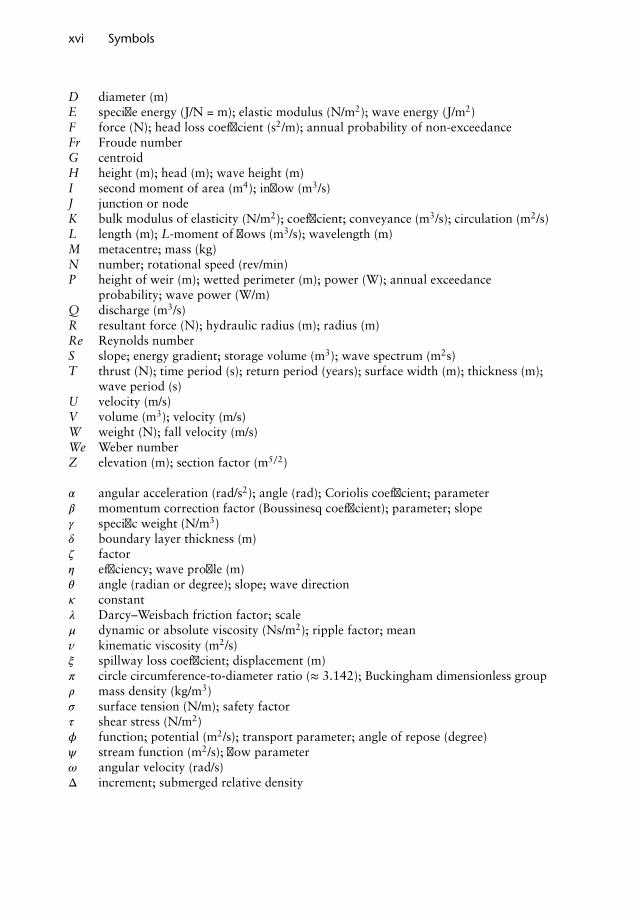
The following is a list of the main symbols used in this book (with their SI units, whereappropriate). Various subscripts have also been used, for example to denote particularlocations. Note that some symbols are inevitably used with different meanings in differentcontexts, and so a number of alternatives are listed below. Readers should be aware ofthis, and check the context for clarification.
a area (m2); distance (m); acceleration (m/s2)b width (m); probability weighted moment of flows (m3/s)c wave celerity (m/s)d diameter (m); water depth (m)f force (N); function; silt factor; frequencyg gravitational acceleration (≈ 9.81 m/s2)h height (m); pressure head difference (m); head loss (m)i rank in descending orderj rank in ascending orderk radius of gyration (m); roughness height (m); constant; coefficientm metacentric height (m); mass (kg)n Manning’s coefficient; exponent; number; wave steepness; group velocity parameterp pressure (N/m2)q discharge per unit width (m2/s)r radius (m); discount rates relative density; distance (m); sinuosity; standard deviation of samplet time (s); L-moment ratiosu velocity (m/s); parameterv velocity (m/s)w velocity (m/s)x distance (m); variabley distance (m); reduced variate; depth (m)z elevation (m); vertical distance (m)
A area (m2)B width (m); centre of buoyancy; benefitC constant; centre of pressure; coefficient; cost
xvi Symbols
D diameter (m)E specifie energy (J/N = m); elastic modulus (N/m2); wave energy (J/m2)F force (N); head loss coefficient (s2/m); annual probability of non-exceedanceFr Froude numberG centroidH height (m); head (m); wave height (m)I second moment of area (m4); inflow (m3/s)J junction or nodeK bulk modulus of elasticity (N/m2); coefficient; conveyance (m3/s); circulation (m2/s)L length (m); L-moment of flows (m3/s); wavelength (m)M metacentre; mass (kg)N number; rotational speed (rev/min)P height of weir (m); wetted perimeter (m); power (W); annual exceedance
probability; wave power (W/m)Q discharge (m3/s)R resultant force (N); hydraulic radius (m); radius (m)Re Reynolds numberS slope; energy gradient; storage volume (m3); wave spectrum (m2s)T thrust (N); time period (s); return period (years); surface width (m); thickness (m);
wave period (s)U velocity (m/s)V volume (m3); velocity (m/s)W weight (N); fall velocity (m/s)We Weber numberZ elevation (m); section factor (m5∕2)
𝛼 angular acceleration (rad/s2); angle (rad); Coriolis coefficient; parameter𝛽 momentum correction factor (Boussinesq coefficient); parameter; slope𝛾 specific weight (N/m3)𝛿 boundary layer thickness (m)𝜁 factor𝜂 efficiency; wave profile (m)𝜃 angle (radian or degree); slope; wave direction𝜅 constant𝜆 Darcy–Weisbach friction factor; scale𝜇 dynamic or absolute viscosity (Ns/m2); ripple factor; meanv kinematic viscosity (m2/s)𝜉 spillway loss coefficient; displacement (m)𝜋 circle circumference-to-diameter ratio (≈ 3.142); Buckingham dimensionless group𝜌 mass density (kg/m3)𝜎 surface tension (N/m); safety factor𝜏 shear stress (N/m2)𝜙 function; potential (m2/s); transport parameter; angle of repose (degree)𝜓 stream function (m2/s); flow parameter𝜔 angular velocity (rad/s)Δ increment; submerged relative density
Chapter 1Properties of Fluids
1.1 Introduction
A fluid is a substance which deforms continuously, or flows, when subjected to shearstresses. The term fluid embraces both gases and liquids; a given mass of liquid will occupya definite volume whereas a gas will fill its container. Gases are readily compressible; thelow compressibility, or elastic volumetric deformation, of liquids is generally neglected incomputations except those relating to large depths in the oceans and in pressure transientsin pipelines.
This text, however, deals exclusively with liquids and more particularly with New-tonian liquids (i.e. those having a linear relationship between shear stress and rate ofdeformation).
Typical values of different properties are quoted in the text as needed for the variousworked examples. For more comprehensive details of physical properties, refer to tablessuch as Kaye and Laby (1995) or internet versions of such information.
1.2 Engineering units
The metre–kilogram–second (mks) system is the agreed version of the international system(SI) of units that is used in this text. The physical quantities in this text can be describedby a set of three primary dimensions (units): mass (kg), length (m) and time (s). Furtherdiscussion is contained in Chapter 9 regarding dimensional analysis. The present chapterrefers to the relevant units that will be used.
The unit of force is called newton (N) and 1 N is the force which accelerates a mass of1 kg at a rate of 1 m/s2 (1 N = 1 kg m/s2).
The unit of work is called joule (J) and it is the energy needed to move a force of 1 Nover a distance of 1 m. Power is the energy or work done per unit time and its unit is watt(W) (1 W = 1 J/s = 1 N m/s).
Nalluri & Featherstone’s Civil Engineering Hydraulics: Essential Theory with Worked Examples,Sixth Edition. Martin Marriott.© 2016 John Wiley & Sons, Ltd. Published 2016 by John Wiley & Sons, Ltd.Companion Website: www.wiley.com/go/Marriott
2 Civil Engineering Hydraulics
1.3 Mass density and specific weight
Mass density (𝜌) or density of a substance is defined as the mass of the substance per unitvolume (kg/m3) and is different from specific weight (𝛾), which is the force exerted by theearth’s gravity (g) upon a unit volume of the substance (𝛾 = 𝜌g: N/m3). In a satellite wherethere is no gravity, an object has no specific weight but possesses the same density that ithas on the earth.
1.4 Relative density
Relative density (s) of a substance is the ratio of its mass density to that of water at astandard temperature (4◦C) and pressure (atmospheric) and is dimensionless.
For water, 𝜌 = 103 kg/m3, 𝛾 = 103 × 9.81 ≃ 104 N/m3 and s = 1.
1.5 Viscosity of fluids
Viscosity is that property of a fluid which by virtue of cohesion and interaction betweenfluid molecules offers resistance to shear deformation. Different fluids deform at differentrates under the action of the same shear stress. Fluids with high viscosity such as syrupdeform relatively more slowly than fluids with low viscosity such as water.
All fluids are viscous and ‘Newtonian fluids’ obey the linear relationship
𝜏 = 𝜇dudy
(Newton’s law of viscosity) [1.1]
where 𝜏 is the shear stress (N/m2), du/dy the velocity gradient or the rate of deformation(rad/s) and 𝜇 the coefficient of dynamic (or absolute) viscosity (N s/m2 or kg/(m s)).
Kinematic viscosity (𝜈) is the ratio of dynamic viscosity to mass density expressed inmetres squared per second.
Water is a Newtonian fluid having a dynamic viscosity of approximately 1.0 × 10⁻³
N s/m2 and kinematic viscosity of 1.0 × 10⁻⁶ m2/s at 20◦C.
1.6 Compressibility and elasticity of fluids
All fluids are compressible under the application of an external force and when the forceis removed they expand back to their original volume, exhibiting the property that stressis proportional to volumetric strain.
The bulk modulus of elasticity,K =pressure change
volumetric strain
= −dp
(dV∕V)[1.2]
The negative sign indicates that an increase in pressure causes a decrease in volume.Water with a bulk modulus of 2.1 × 10⁹ N/m2 at 20◦C is 100 times more compressible
than steel, but it is ordinarily considered incompressible.
1.7 Vapour pressure of liquids
A liquid in a closed container is subjected to partial vapour pressure due to the escapingmolecules from the surface; it reaches a stage of equilibrium when this pressure reaches
Ch
apter
1
Properties of Fluids 3
saturated vapour pressure. Since this depends upon molecular activity, which is a functionof temperature, the vapour pressure of a fluid also depends upon its temperature andincreases with it. If the pressure above a liquid reaches the vapour pressure of the liquid,boiling occurs; for example, if the pressure is reduced sufficiently, boiling may occur atroom temperature.
The saturated vapour pressure for water at 20◦C is 2.45 × 10³ N/m2.
1.8 Surface tension and capillarity
Liquids possess the properties of cohesion and adhesion due to molecular attraction. Dueto the property of cohesion, liquids can resist small tensile forces at the interface betweenthe liquid and air, known as surface tension (𝜎: N/m). If the liquid molecules have greateradhesion than cohesion, then the liquid sticks to the surface of the container with which itis in contact, resulting in a capillary rise of the liquid surface; a predominating cohesion,in contrast, causes capillary depression. The surface tension of water is 73 × 10−3 N/mat 20◦C.
The capillary rise or depression h of a liquid in a tube of diameter d can be written as
h = 4𝜎 cos 𝜃𝜌gd
[1.3]
where 𝜃 is the angle of contact between liquid and solid.Surface tension increases the pressure within a droplet of liquid. The internal pressure
p balancing the surface tensional force of a small spherical droplet of radius r is given by
p = 2𝜎r
[1.4]
Worked examples
Example 1.1
The density of an oil at 20◦C is 850 kg/m3. Find its relative density and kinematic viscosityif the dynamic viscosity is 5 × 10⁻³ kg/(m s).
Solution:
Relative density, s = 𝜌of oil𝜌of water
= 850103
= 0.85
Kinematic viscosity,𝜈 = 𝜇
𝜌
= 5 × 10⁻³
850= 5.88 × 10⁻⁶ m2∕s
Ch
apte
r1
4 Civil Engineering Hydraulics
Example 1.2
If the velocity distribution of a viscous liquid (𝜇 = 0.9 N s/m2) over a fixed boundary isgiven by u = 0.68y − y2, in which u is the velocity (in metres per second) at a distance y(in metres) above the boundary surface, determine the shear stress at the surface and aty = 0.34 m.
Solution:
u = 0.68y − y2
⇒dudy
= 0.68 − 2y
Hence, (du∕dy)y=0 = 0.68 s−1 and (du∕dy)y=0.34m = 0.
Dynamic viscosity of the fluid,𝜇 = 0.9 N s∕m2
From Equation 1.1,
shear stress (𝜏)y=0 = 0.9 × 0.68
= 0.612 N∕m2
and at y = 0.34 m, 𝜏 = 0.
Example 1.3
At a depth of 8.5 km in the ocean the pressure is 90 MN/m2. The specific weight of thesea water at the surface is 10.2 kN/m3 and its average bulk modulus is 2.4 × 10⁶ kN/m2.Determine (a) the change in specific volume, (b) the specific volume and (c) the specificweight of sea water at 8.5 km depth.
Solution:
Change in pressure at a depth of 8.5 km,dp = 90 MN∕m2
= 9 × 10⁴ kN∕m2
Bulk modulus,K = 2.4 × 10⁶ kN∕m2
From K = −dp
(dV∕V)
dVV
= −9 × 10⁴
2.4 × 106= −3.75 × 10⁻²
Defining specific volume as 1/ 𝛾 (m3/kN), the specific volume of sea water at the surface =1/10.2 = 9.8 × 10⁻² m3/kN.
Change in specific volume between that
at the surface and at 8.5 km depth,dV
= −3.75 × 10−2 × 9.8 × 10−2
= −36.75 × 10⁻⁴ m3∕kN
Ch
apter
1
Properties of Fluids 5
The specific volume of sea water at 8.5 km depth = 9.8 × 10⁻² − 36.75 × 10−4
= 9.44 × 10⁻² m3∕kN
The specific weight of sea water at 8.5 km depth = 1specific volume
= 19.44 × 10−2
= 10.6 kN∕m3
References and recommended reading
Kaye, G. W. C. and Laby, T. H. (1995) Tables of Physical and Chemical Constants, 16th edn,Longman, London. http://www.kayelaby.npl.co.uk
Massey, B. S. and Ward-Smith, J. (2012) Mechanics of Fluids, 9th edn, Taylor & Francis,Abingdon, UK.
Problems
1. (a) Explain why the viscosity of a liquid decreases while that of a gas increases with anincrease of temperature.
(b) The following data refer to a liquid under shearing action at a constant temperature.Determine its dynamic viscosity.
du/dy (s−1) 0 0.2 0.4 0.6 0.8𝜏 (N/m2) 0 0 1.9 3.1 4.0
2. A 300 mm wide shaft sleeve moves along a 100 mm diameter shaft at a speed of 0.5 m/sunder the application of a force of 250 N in the direction of its motion. If 1000 N of forceis applied, what speed will the sleeve attain? Assume the temperature of the sleeve to beconstant and determine the viscosity of the Newtonian fluid in the clearance between theshaft and its sleeve if the radial clearance is estimated to be 0.075 mm.
3. A shaft of 100 mm diameter rotates at 120 rad/s in a bearing 150 mm long. If the radialclearance is 0.2 mm and the absolute viscosity of the lubricant is 0.20 kg/(m s), find thepower loss in the bearing.
4. A block of dimensions 300 mm × 300 mm × 300 mm and mass 30 kg slides down a planeinclined at 30◦ to the horizontal, on which there is a thin film of oil of viscosity 2.3 × 10⁻³
N s/m2. Determine the speed of the block if the film thickness is estimated to be 0.03 mm.
5. Calculate the capillary effect (in millimetres) in a glass tube of 6 mm diameter whenimmersed in (i) water and (ii) mercury, both liquids being at 20◦C. Assume 𝜎 to be 73× 10−3
N/m for water and 0.5 N/m for mercury. The contact angles for water and mercury are0 and 130◦, respectively.
6. Calculate the internal pressure of a 25 mm diameter soap bubble if the tension in the soapfilm is 0.5 N/m.
Ch
apte
r1

Chapter 2Fluid Statics
2.1 Introduction
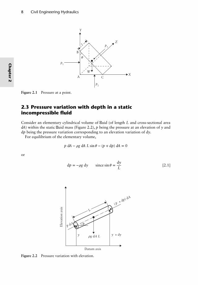
Fluid statics is the study of pressures throughout a fluid at rest and the pressure forces onfinite surfaces. Since the fluid is at rest there are no shear stresses in it. Hence the pressure pat a point on a plane surface (inside the fluid or on the boundaries of its container), definedas the limiting value of the ratio of normal force to surface area as the area approacheszero size, always acts normal to the surface and is measured in newtons per square metre(pascals, Pa) or in bars (1 bar = 105 N/m2 or 105 Pa).
2.2 Pascal’s law
Pascal’s law states that the pressure at a point in a fluid at rest is the same in all directions.This means it is independent of the orientation of the surface around the point.
Consider a small triangular prism of unit length surrounding the point in a fluid at rest(Figure 2.1).
Since the body is in static equilibrium, we can write
p1(AB × l) − p3(BC × l) cos 𝜃 = 0 (i)
and
p2(AC × l) − p3(BC × l) sin 𝜃 − W = 0 (ii)
From Equation (i) p1 = p3, since cos 𝜃 = AB∕BC, and Equation (ii) gives p2 = p3, sincesin 𝜃 = AC∕BC and W = 0 as the prism shrinks to a point.
⇒ p1 = p2 = p3
Nalluri & Featherstone’s Civil Engineering Hydraulics: Essential Theory with Worked Examples,Sixth Edition. Martin Marriott.© 2016 John Wiley & Sons, Ltd. Published 2016 by John Wiley & Sons, Ltd.Companion Website: www.wiley.com/go/Marriott
8 Civil Engineering Hydraulics
Y
B
A C
W
p1
p2
p3
Z
θ
X
l
Figure 2.1 Pressure at a point.
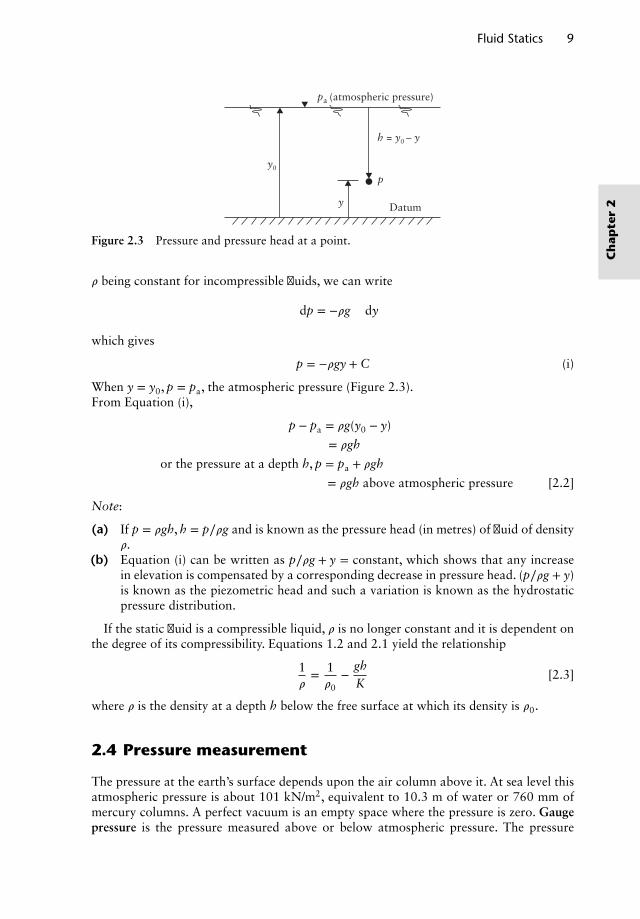
2.3 Pressure variation with depth in a staticincompressible fluid
Consider an elementary cylindrical volume of fluid (of length L and cross-sectional areadA) within the static fluid mass (Figure 2.2), p being the pressure at an elevation of y anddp being the pressure variation corresponding to an elevation variation of dy.
For equilibrium of the elementary volume,
p dA − 𝜌g dA L sin 𝜃 − (p + dp) dA = 0
or
dp = −𝜌g dy(
since sin 𝜃 =dyL
)[2.1]
Ele
vati
on a
xis
Datum axis
y + dy g dA L
θ
( p + dp) dA
y
p dA
L
ρ
Figure 2.2 Pressure variation with elevation.
Ch
apter
2
Fluid Statics 9
pa (atmospheric pressure)
y0
y
p
Datum
h = y0 – y
Figure 2.3 Pressure and pressure head at a point.
𝜌 being constant for incompressible fluids, we can write
∫ dp = −𝜌g∫ dy
which gives
p = −𝜌gy + C (i)
When y = y0, p = pa, the atmospheric pressure (Figure 2.3).From Equation (i),
p − pa = 𝜌g(y0 − y)
= 𝜌gh
or the pressure at a depth h, p = pa + 𝜌gh
= 𝜌gh above atmospheric pressure [2.2]
Note:
(a) If p = 𝜌gh, h = p∕𝜌g and is known as the pressure head (in metres) of fluid of density𝜌.
(b) Equation (i) can be written as p∕𝜌g + y = constant, which shows that any increasein elevation is compensated by a corresponding decrease in pressure head. (p∕𝜌g + y)is known as the piezometric head and such a variation is known as the hydrostaticpressure distribution.
If the static fluid is a compressible liquid, 𝜌 is no longer constant and it is dependent onthe degree of its compressibility. Equations 1.2 and 2.1 yield the relationship
1𝜌= 1𝜌0
−ghK
[2.3]
where 𝜌 is the density at a depth h below the free surface at which its density is 𝜌0.
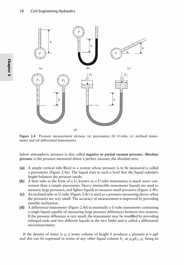
2.4 Pressure measurement
The pressure at the earth’s surface depends upon the air column above it. At sea level thisatmospheric pressure is about 101 kN/m2, equivalent to 10.3 m of water or 760 mm ofmercury columns. A perfect vacuum is an empty space where the pressure is zero. Gaugepressure is the pressure measured above or below atmospheric pressure. The pressure
Ch
apte
r2
10 Civil Engineering Hydraulics
Figure 2.4 Pressure measurement devices: (a) piezometer, (b) U-tube, (c) inclined mano-meter and (d) differential manometers.
below atmospheric pressure is also called negative or partial vacuum pressure. Absolutepressure is the pressure measured above a perfect vacuum, the absolute zero.
(a) A simple vertical tube fixed to a system whose pressure is to be measured is calleda piezometer (Figure 2.4a). The liquid rises to such a level that the liquid column’sheight balances the pressure inside.
(b) A bent tube in the form of a U, known as a U-tube manometer, is much more con-venient than a simple piezometer. Heavy immiscible manometer liquids are used tomeasure large pressures, and lighter liquids to measure small pressures (Figure 2.4b).
(c) An inclined tube or U-tube (Figure 2.4c) is used as a pressure-measuring device whenthe pressures are very small. The accuracy of measurement is improved by providingsuitable inclination.
(d) A differential manometer (Figure 2.4d) is essentially a U-tube manometer containinga single liquid capable of measuring large pressure differences between two systems.If the pressure difference is very small, the manometer may be modified by providingenlarged ends and two different liquids in the two limbs and is called a differentialmicromanometer.
If the density of water is 𝜌, a water column of height h produces a pressure p = 𝜌ghand this can be expressed in terms of any other liquid column h1 as 𝜌1gh1, 𝜌1 being its
Ch
apter
2
Fluid Statics 11
density:
⇒ h in water column =(𝜌1
𝜌
)h1 = sh1 [2.4]
where s is the relative density of the liquid.For each one of the pressure measurement devices shown in Figure 2.4, an equation can
be written using the principle of hydrostatic pressure distribution, expressing the pressures(in metres) of the water column (Equation 2.4) for convenience.
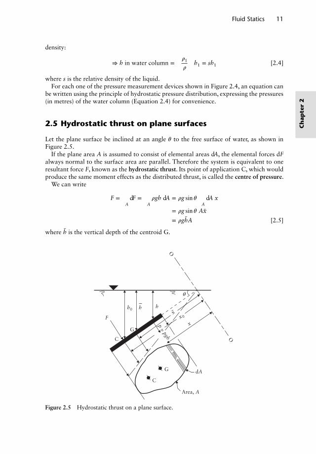
2.5 Hydrostatic thrust on plane surfaces
Let the plane surface be inclined at an angle 𝜃 to the free surface of water, as shown inFigure 2.5.
If the plane area A is assumed to consist of elemental areas dA, the elemental forces dFalways normal to the surface area are parallel. Therefore the system is equivalent to oneresultant force F, known as the hydrostatic thrust. Its point of application C, which wouldproduce the same moment effects as the distributed thrust, is called the centre of pressure.
We can write
F = ∫AdF = ∫A
𝜌gh dA = 𝜌g sin 𝜃 ∫AdA x
= 𝜌g sin 𝜃 Ax
= 𝜌ghA [2.5]
where h is the vertical depth of the centroid G.
F
hh0
dA
p = pgh
Area, A
G
G
O
O
C
C
h
θ
x
x 0
x
Figure 2.5 Hydrostatic thrust on a plane surface.
Ch
apte
r2
12 Civil Engineering Hydraulics
Area, A
G
h
F = ρghAC
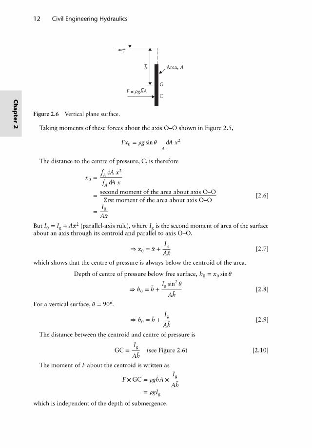
Figure 2.6 Vertical plane surface.
Taking moments of these forces about the axis O–O shown in Figure 2.5,
Fx0 = 𝜌g sin 𝜃 ∫AdA x2
The distance to the centre of pressure, C, is therefore
x0 =∫A dA x2
∫A dA x
= second moment of the area about axis O–Ofirst moment of the area about axis O–O
[2.6]
=I0
Ax
But I0 = Ig + Ax2 (parallel-axis rule), where Ig is the second moment of area of the surfaceabout an axis through its centroid and parallel to axis O–O.
⇒ x0 = x +Ig
Ax[2.7]
which shows that the centre of pressure is always below the centroid of the area.
Depth of centre of pressure below free surface, h0 = x0 sin 𝜃
⇒ h0 = h +Ig sin
2𝜃
Ah[2.8]
For a vertical surface, 𝜃 = 90◦.
⇒ h0 = h +Ig
Ah[2.9]
The distance between the centroid and centre of pressure is
GC =Ig
Ah(see Figure 2.6) [2.10]
The moment of F about the centroid is written as
F × GC = 𝜌ghA ×Ig
Ah= 𝜌gIg
which is independent of the depth of submergence.
Ch
apter
2
Fluid Statics 13
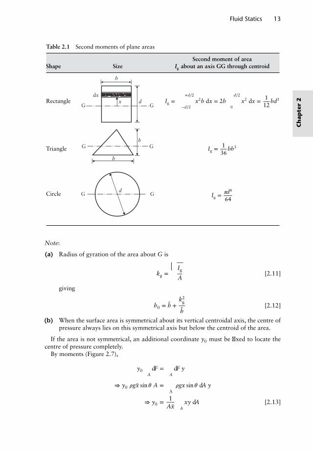
Table 2.1 Second moments of plane areas
Second moment of areaShape Size Ig about an axis GG through centroid
RectangleG G
dxdx
b
Ig = ∫+d∕2
−d∕2x2b dx = 2b∫
d∕2
0x2 dx = 1
12bd3
Triangle
h
b
GG Ig =136
bh3
Circle GGd
Ig =𝜋d4
64
Note:
(a) Radius of gyration of the area about G is
kg =
√Ig
A[2.11]
giving
h0 = h +k2
g
h[2.12]
(b) When the surface area is symmetrical about its vertical centroidal axis, the centre ofpressure always lies on this symmetrical axis but below the centroid of the area.
If the area is not symmetrical, an additional coordinate y0 must be fixed to locate thecentre of pressure completely.
By moments (Figure 2.7),
y0 ∫AdF = ∫A
dF y
⇒ y0 𝜌gx sin 𝜃 A = ∫A𝜌gx sin 𝜃 dA y
⇒ y0 = 1Ax ∫A
xy dA [2.13]
Ch
apte
r2
14 Civil Engineering Hydraulics
OO
GCy0
x0x
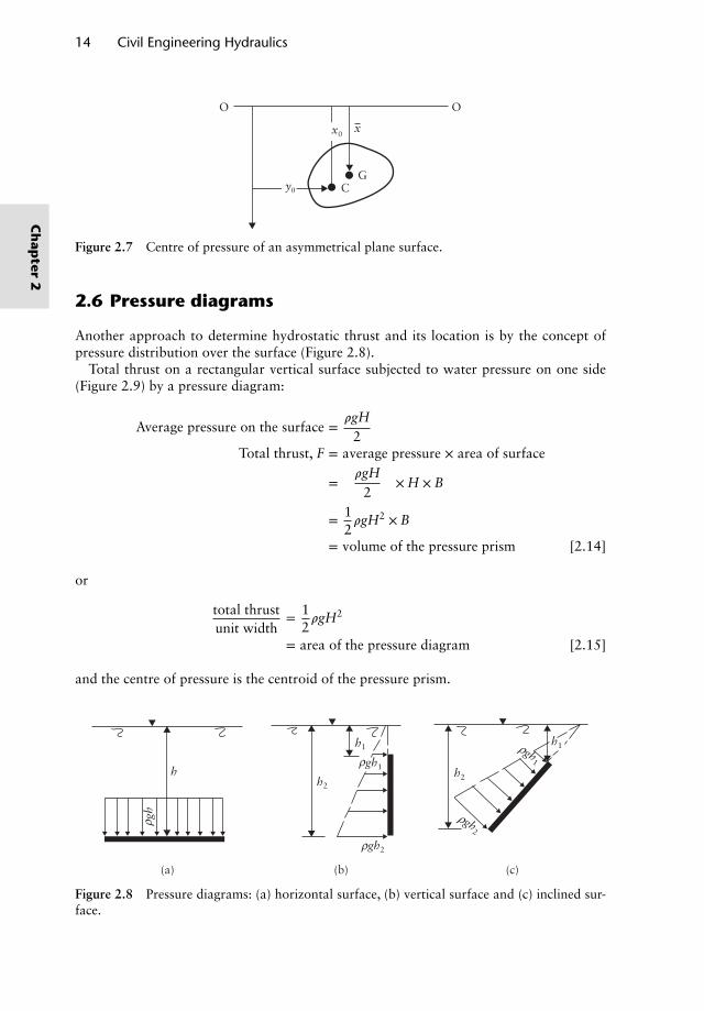
Figure 2.7 Centre of pressure of an asymmetrical plane surface.
2.6 Pressure diagrams
Another approach to determine hydrostatic thrust and its location is by the concept ofpressure distribution over the surface (Figure 2.8).
Total thrust on a rectangular vertical surface subjected to water pressure on one side(Figure 2.9) by a pressure diagram:
Average pressure on the surface =𝜌gH
2Total thrust, F = average pressure × area of surface
=(𝜌gH
2
)× H × B
= 12𝜌gH2 × B
= volume of the pressure prism [2.14]
or
total thrustunit width
= 12𝜌gH2
= area of the pressure diagram [2.15]
and the centre of pressure is the centroid of the pressure prism.
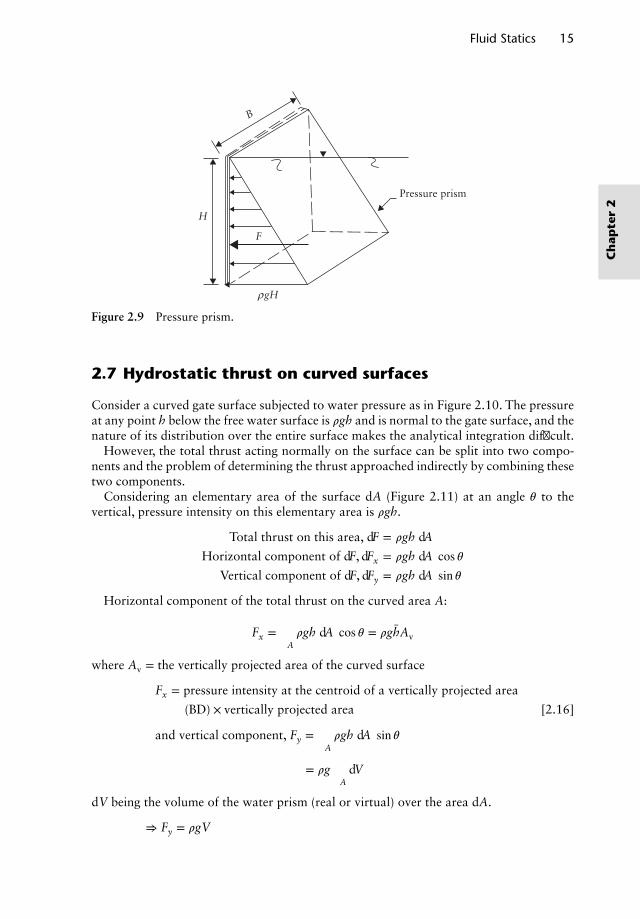
(c)(b)(a)
hh2
h2
gh1
gh1
gh2
gh2
gh
h1 h1
ρ
ρ
ρ
ρ
ρ
Figure 2.8 Pressure diagrams: (a) horizontal surface, (b) vertical surface and (c) inclined sur-face.
Ch
apter
2
Fluid Statics 15
Pressure prism
B
H
F
ρgH
Figure 2.9 Pressure prism.
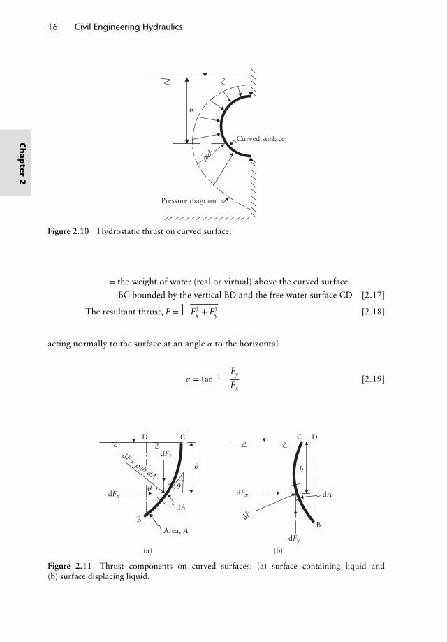
2.7 Hydrostatic thrust on curved surfaces
Consider a curved gate surface subjected to water pressure as in Figure 2.10. The pressureat any point h below the free water surface is 𝜌gh and is normal to the gate surface, and thenature of its distribution over the entire surface makes the analytical integration difficult.
However, the total thrust acting normally on the surface can be split into two compo-nents and the problem of determining the thrust approached indirectly by combining thesetwo components.
Considering an elementary area of the surface dA (Figure 2.11) at an angle 𝜃 to thevertical, pressure intensity on this elementary area is 𝜌gh.
Total thrust on this area, dF = 𝜌gh dA
Horizontal component of dF, dFx = 𝜌gh dA cos 𝜃Vertical component of dF, dFy = 𝜌gh dA sin 𝜃
Horizontal component of the total thrust on the curved area A:
Fx = ∫A𝜌gh dA cos 𝜃 = 𝜌ghAv
where Av = the vertically projected area of the curved surface
Fx = pressure intensity at the centroid of a vertically projected area
(BD) × vertically projected area [2.16]
and vertical component, Fy = ∫A𝜌gh dA sin 𝜃
= 𝜌g∫AdV
dV being the volume of the water prism (real or virtual) over the area dA.
⇒ Fy = 𝜌gV
Ch
apte
r2
16 Civil Engineering Hydraulics
Curved surface
Pressure diagram
h
ghρ
Figure 2.10 Hydrostatic thrust on curved surface.
= the weight of water (real or virtual) above the curved surface
BC bounded by the vertical BD and the free water surface CD [2.17]
The resultant thrust, F =√
F2x + F2
y [2.18]
acting normally to the surface at an angle 𝛼 to the horizontal
𝛼 = tan−1(Fy
Fx
)[2.19]
(b)(a)
Area, A
B
C
θθ
C
hh
D
dF = gh dA
D
dA
dAdF
B
dFy
dFy
dFxdFx
ρ
Figure 2.11 Thrust components on curved surfaces: (a) surface containing liquid and(b) surface displacing liquid.
Ch
apter
2
Fluid Statics 17
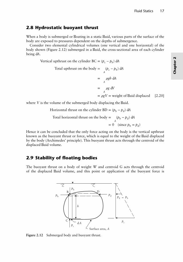
2.8 Hydrostatic buoyant thrust
When a body is submerged or floating in a static fluid, various parts of the surface of thebody are exposed to pressures dependent on the depths of submergence.
Consider two elemental cylindrical volumes (one vertical and one horizontal) of thebody shown (Figure 2.12) submerged in a fluid, the cross-sectional area of each cylinderbeing dA.
Vertical upthrust on the cylinder BC = (pc − pb) dA
Total upthrust on the body = ∫A(pc − pb) dA
= ∫A𝜌gh dA
= ∫A𝜌g dV
= 𝜌gV = weight of fluid displaced [2.20]
where V is the volume of the submerged body displacing the fluid.
Horizontal thrust on the cylinder BD = (pb − pd) dA
Total horizontal thrust on the body = ∫A(pb − pd) dA
= 0 (since pb = pd)
Hence it can be concluded that the only force acting on the body is the vertical upthrustknown as the buoyant thrust or force, which is equal to the weight of the fluid displacedby the body (Archimedes’ principle). This buoyant thrust acts through the centroid of thedisplaced fluid volume.
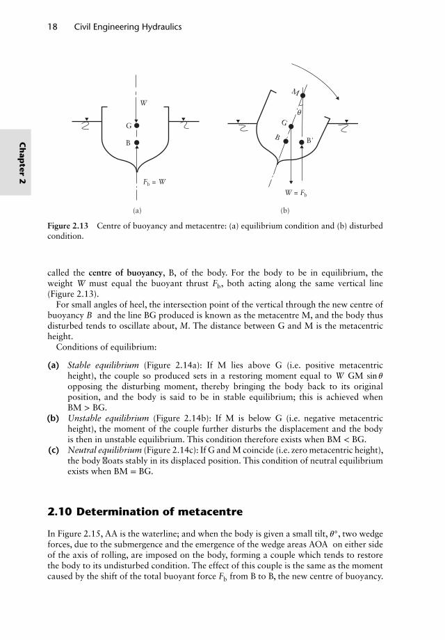
2.9 Stability of floating bodies
The buoyant thrust on a body of weight W and centroid G acts through the centroidof the displaced fluid volume, and this point or application of the buoyant force is
B D
=
Surface area, A
dAC
h
pd pd pbpb
pb
pcpc
Figure 2.12 Submerged body and buoyant thrust.
Ch
apte
r2
18 Civil Engineering Hydraulics
G
Fb = W
W = Fb
B'
Wθ
B
(b)(a)
B
G
M
Figure 2.13 Centre of buoyancy and metacentre: (a) equilibrium condition and (b) disturbedcondition.
called the centre of buoyancy, B, of the body. For the body to be in equilibrium, theweight W must equal the buoyant thrust Fb, both acting along the same vertical line(Figure 2.13).
For small angles of heel, the intersection point of the vertical through the new centre ofbuoyancy B′ and the line BG produced is known as the metacentre M, and the body thusdisturbed tends to oscillate about, M. The distance between G and M is the metacentricheight.
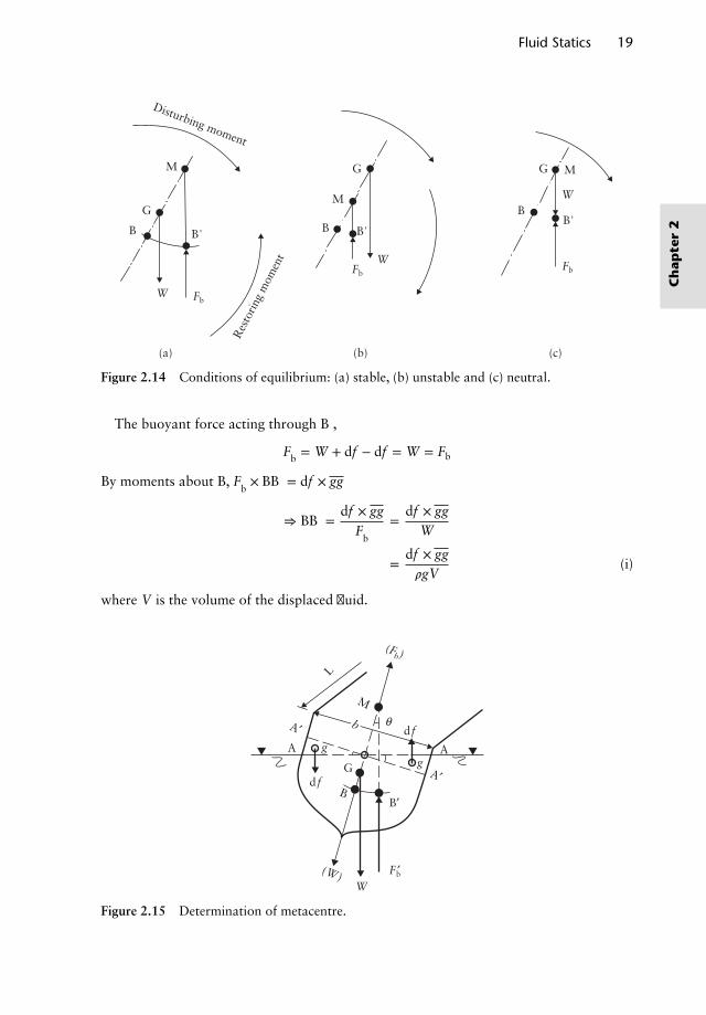
Conditions of equilibrium:
(a) Stable equilibrium (Figure 2.14a): If M lies above G (i.e. positive metacentricheight), the couple so produced sets in a restoring moment equal to W GM sin 𝜃opposing the disturbing moment, thereby bringing the body back to its originalposition, and the body is said to be in stable equilibrium; this is achieved whenBM > BG.
(b) Unstable equilibrium (Figure 2.14b): If M is below G (i.e. negative metacentricheight), the moment of the couple further disturbs the displacement and the bodyis then in unstable equilibrium. This condition therefore exists when BM < BG.
(c) Neutral equilibrium (Figure 2.14c): If G and M coincide (i.e. zero metacentric height),the body floats stably in its displaced position. This condition of neutral equilibriumexists when BM = BG.
2.10 Determination of metacentre
In Figure 2.15, AA is the waterline; and when the body is given a small tilt, 𝜃◦, two wedgeforces, due to the submergence and the emergence of the wedge areas AOA′ on either sideof the axis of rolling, are imposed on the body, forming a couple which tends to restorethe body to its undisturbed condition. The effect of this couple is the same as the momentcaused by the shift of the total buoyant force Fb from B to B′, the new centre of buoyancy.
Ch
apter
2
Fluid Statics 19
G
GGM
Disturbing moment
Res
tori
ng m
omen
t
M
M
Fb
FbFb
B' B'B'
W
W
W
B B
B
(c)(b)(a)
Figure 2.14 Conditions of equilibrium: (a) stable, (b) unstable and (c) neutral.
The buoyant force acting through B′,
F′b = W + df − df = W = Fb
By moments about B, F′b× BB′ = df × gg
⇒ BB′ =df × gg
F′b
=df × gg
W
=df × gg𝜌gV
(i)
where V is the volume of the displaced fluid.
F ′b
(Fb)
(W )
B′
G
A A
d f
d f
gg
B
A′
A′
W
θ
M
L
b
Figure 2.15 Determination of metacentre.
Ch
apte
r2
20 Civil Engineering Hydraulics
The wedge force df = 𝜌g × 12AA′ × 1
2b × L (for small angles), where L is the length of
the body.
AA′ = 12
b𝜃 and gg = 23
(12
b)+ 2
3
(12
b)
= 23
b
⇒ BB′ = BM𝜃 =𝜌g × 1
4b𝜃 × 1
2b × L × 2
3b
𝜌gV(from Equation (i))
or
BM = 112
Lb3
V= I
V[2.21]
where I is the second moment of the plan area of the body at water level about its longi-tudinal axis.
Hence the metacentric height, GM = BM − BG
= IV
− BG [2.22]
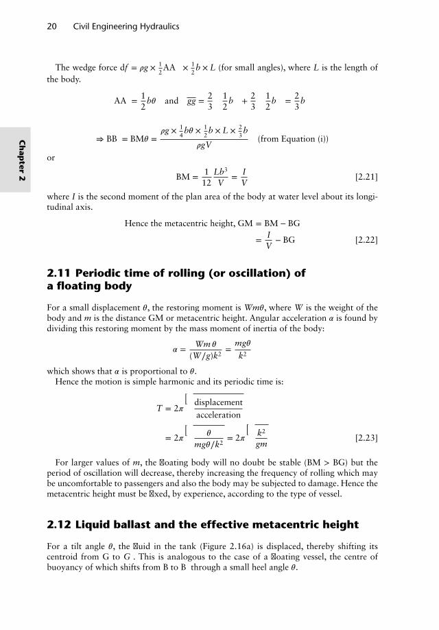
2.11 Periodic time of rolling (or oscillation) ofa floating body
For a small displacement 𝜃, the restoring moment is Wm𝜃, where W is the weight of thebody and m is the distance GM or metacentric height. Angular acceleration 𝛼 is found bydividing this restoring moment by the mass moment of inertia of the body:
𝛼 = Wm 𝜃
(W∕g)k2=
mg𝜃
k2
which shows that 𝛼 is proportional to 𝜃.Hence the motion is simple harmonic and its periodic time is:
T = 2𝜋
√displacement
acceleration
= 2𝜋
√𝜃
mg𝜃∕k2= 2𝜋
√k2
gm[2.23]
For larger values of m, the floating body will no doubt be stable (BM > BG) but theperiod of oscillation will decrease, thereby increasing the frequency of rolling which maybe uncomfortable to passengers and also the body may be subjected to damage. Hence themetacentric height must be fixed, by experience, according to the type of vessel.
2.12 Liquid ballast and the effective metacentric height
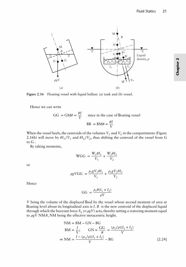
For a tilt angle 𝜃, the fluid in the tank (Figure 2.16a) is displaced, thereby shifting itscentroid from G to G′. This is analogous to the case of a floating vessel, the centre ofbuoyancy of which shifts from B to B′ through a small heel angle 𝜃.
Ch
apter
2
Fluid Statics 21
θ
θ
gV
ρ1,V1
I2I1
WFb
M
Liquiddensity, ρ
N
BG'
G'
B'G
(b)(a)
G
M
ρ1,V2
ρ
Figure 2.16 Floating vessel with liquid ballast: (a) tank and (b) vessel.
Hence we can write
GG′ = GM𝜃 = 𝜃IV
(since in the case of floating vessel
BB′ = BM𝜃 = 𝜃IV
)When the vessel heels, the centroids of the volumes V1 and V2 in the compartments (Figure2.16b) will move by 𝜃I1∕V1 and 𝜃I2∕V2, thus shifting the centroid of the vessel from Gto G′.
By taking moments,
WGG′ =W1𝜃I1
V1+
W2𝜃I2
V2
or
𝜌gVGG′ =𝜌1gV1𝜃I1
V1+𝜌1gV2𝜃I2
V2
Hence
GG′ =𝜌1𝜃(I1 + I2)
𝜌V
V being the volume of the displaced fluid by the vessel whose second moment of area atfloating level about its longitudinal axis is I. B′ is the new centroid of the displaced liquidthrough which the buoyant force Fb (=𝜌gV) acts, thereby setting a restoring moment equalto 𝜌gV NM 𝜃, NM being the effective metacentric height.
NM = BM − GN − BG
BM = IV
; GN = GG′
𝜃=
(𝜌1∕𝜌)(I1 + I2)V
⇒ NM =I − (𝜌1∕𝜌)(I1 + I2)
V− BG [2.24]
Ch
apte
r2
22 Civil Engineering Hydraulics
and if 𝜌1 = 𝜌,
NM =I − (I1 + I2)
V− BG
2.13 Relative equilibrium
If a body of fluid is subjected to motion such that no layer moves relative to an adjacentlayer, shear stresses do not exist within the fluid. In other words, in a moving fluid mass ifthe fluid particles do not move relative to each other, they are said to be in static conditionand a relative or dynamic equilibrium exists between them under the action of acceleratingforce, and fluid pressures are everywhere normal to the surfaces on which they act.
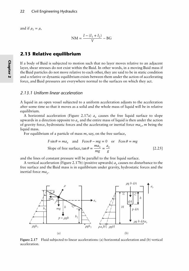
2.13.1 Uniform linear acceleration
A liquid in an open vessel subjected to a uniform acceleration adjusts to the accelerationafter some time so that it moves as a solid and the whole mass of liquid will be in relativeequilibrium.
A horizontal acceleration (Figure 2.17a) ax causes the free liquid surface to slopeupwards in a direction opposite to ax and the entire mass of liquid is then under the actionof gravity force, hydrostatic forces and the accelerating or inertial force max, m being theliquid mass.
For equilibrium of a particle of mass m, say, on the free surface,
F sin 𝜃 = max and Fcos 𝜃 − mg = 0 or Fcos 𝜃 = mg
Slope of free surface, tan 𝜃 =max
mg=
ax
g[2.25]
and the lines of constant pressure will be parallel to the free liquid surface.A vertical acceleration (Figure 2.17b) (positive upwards) ay causes no disturbance to the
free surface and the fluid mass is in equilibrium under gravity, hydrostatic forces and theinertial force may.
gh1 gh2 ayH gH
g h dA
p = gh
ay
axmax
θ
h2
h1hmg
F
dA
(b)(a)
p dAH
h
g h dAay
ρ
ρ
ρ ρ ρρ
ρ
Figure 2.17 Fluid subjected to linear accelerations: (a) horizontal acceleration and (b) verticalacceleration.
Ch
apter
2
Fluid Statics 23
For equilibrium of a small column of liquid of area dA,
p dA = 𝜌h dA g + 𝜌h dA ay
The pressure intensity at a depth h below the free surface is
p = 𝜌gh(
1 +ay
g
)[2.26]
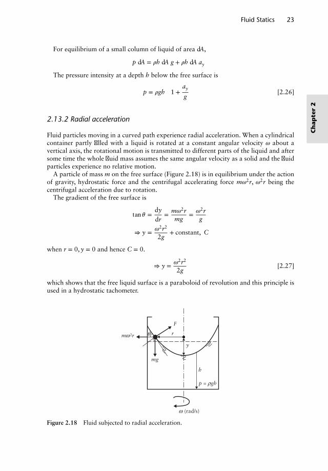
2.13.2 Radial acceleration
Fluid particles moving in a curved path experience radial acceleration. When a cylindricalcontainer partly filled with a liquid is rotated at a constant angular velocity 𝜔 about avertical axis, the rotational motion is transmitted to different parts of the liquid and aftersome time the whole fluid mass assumes the same angular velocity as a solid and the fluidparticles experience no relative motion.
A particle of mass m on the free surface (Figure 2.18) is in equilibrium under the actionof gravity, hydrostatic force and the centrifugal accelerating force m𝜔2r, 𝜔2r being thecentrifugal acceleration due to rotation.
The gradient of the free surface is
tan 𝜃 =dy
dr= m𝜔2r
mg= 𝜔2r
g
⇒ y = 𝜔2r2
2g+ constant, C
when r = 0, y = 0 and hence C = 0.
⇒ y = 𝜔2r2
2g[2.27]
which shows that the free liquid surface is a paraboloid of revolution and this principle isused in a hydrostatic tachometer.
F
r
y
h
mg
mω 2r θ
ω (rad/s)
p = ρgh
Figure 2.18 Fluid subjected to radial acceleration.
Ch
apte
r2
24 Civil Engineering Hydraulics
Worked examples
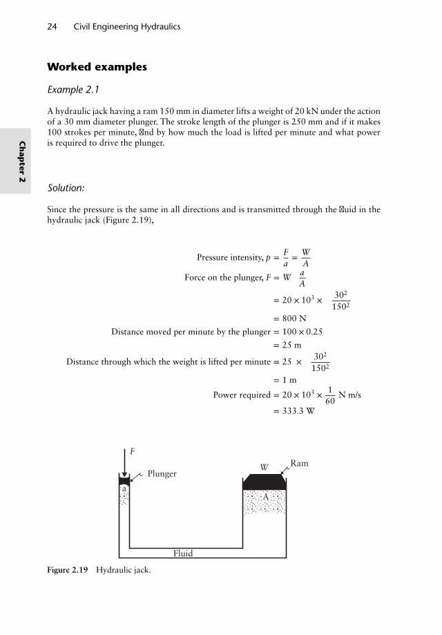
Example 2.1
A hydraulic jack having a ram 150 mm in diameter lifts a weight of 20 kN under the actionof a 30 mm diameter plunger. The stroke length of the plunger is 250 mm and if it makes100 strokes per minute, find by how much the load is lifted per minute and what poweris required to drive the plunger.
Solution:
Since the pressure is the same in all directions and is transmitted through the fluid in thehydraulic jack (Figure 2.19),
Pressure intensity, p = Fa= W
A
Force on the plunger, F = W( a
A
)= 20 × 103 ×
(302
1502
)= 800 N
Distance moved per minute by the plunger = 100 × 0.25
= 25 m
Distance through which the weight is lifted per minute = 25 ×(
302
1502
)= 1 m
Power required = 20 × 103 × 160
N m/s
= 333.3 W
Fluid
RamPlunger
F
W
aA
Figure 2.19 Hydraulic jack.
Ch
apter
2
Fluid Statics 25
pa
p p
x
400
mm
200
mm 30
0 m
m
(b)(a)
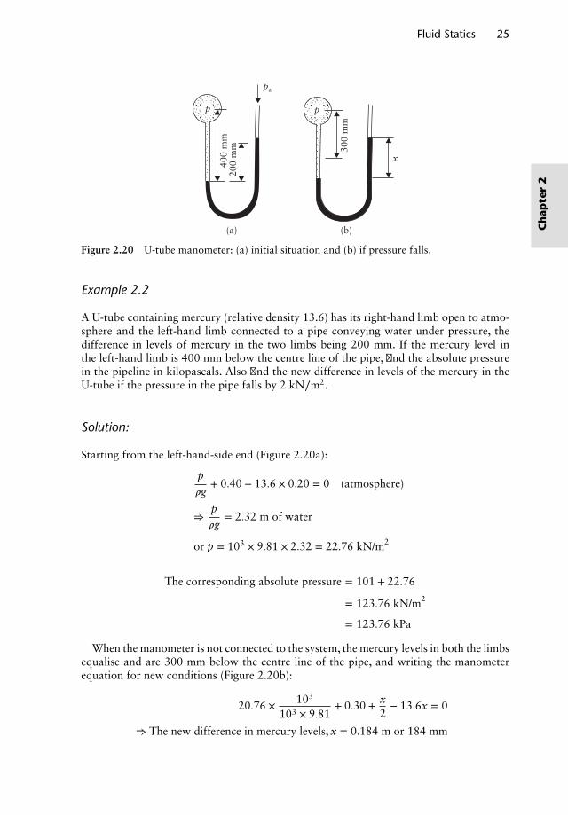
Figure 2.20 U-tube manometer: (a) initial situation and (b) if pressure falls.
Example 2.2
A U-tube containing mercury (relative density 13.6) has its right-hand limb open to atmo-sphere and the left-hand limb connected to a pipe conveying water under pressure, thedifference in levels of mercury in the two limbs being 200 mm. If the mercury level inthe left-hand limb is 400 mm below the centre line of the pipe, find the absolute pressurein the pipeline in kilopascals. Also find the new difference in levels of the mercury in theU-tube if the pressure in the pipe falls by 2 kN∕m2.
Solution:
Starting from the left-hand-side end (Figure 2.20a):
p𝜌g
+ 0.40 − 13.6 × 0.20 = 0 (atmosphere)
⇒p𝜌g
= 2.32 m of water
or p = 103 × 9.81 × 2.32 = 22.76 kN/m2
The corresponding absolute pressure = 101 + 22.76
= 123.76 kN/m2
= 123.76 kPa
When the manometer is not connected to the system, the mercury levels in both the limbsequalise and are 300 mm below the centre line of the pipe, and writing the manometerequation for new conditions (Figure 2.20b):
20.76 × 10³
103 × 9.81+ 0.30 + x
2− 13.6x = 0
⇒ The new difference in mercury levels, x = 0.184 m or 184 mm
Ch
apte
r2
26 Civil Engineering Hydraulics
Oil
50 mm
dx
Water
Area, a
Area, A
dxp2p1
0
0
h0
0
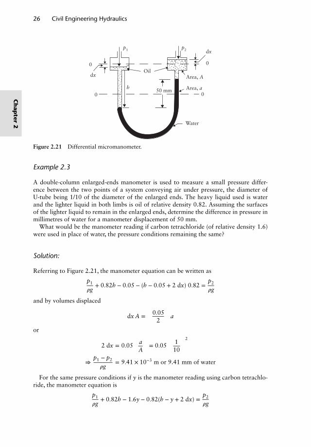
Figure 2.21 Differential micromanometer.
Example 2.3
A double-column enlarged-ends manometer is used to measure a small pressure differ-ence between the two points of a system conveying air under pressure, the diameter ofU-tube being 1/10 of the diameter of the enlarged ends. The heavy liquid used is waterand the lighter liquid in both limbs is oil of relative density 0.82. Assuming the surfacesof the lighter liquid to remain in the enlarged ends, determine the difference in pressure inmillimetres of water for a manometer displacement of 50 mm.
What would be the manometer reading if carbon tetrachloride (of relative density 1.6)were used in place of water, the pressure conditions remaining the same?
Solution:
Referring to Figure 2.21, the manometer equation can be written as
p1
𝜌g+ 0.82h − 0.05 − (h − 0.05 + 2 dx) 0.82 =
p2
𝜌g
and by volumes displaced
dx A =(
0.052
)a
or
2 dx = 0.05( a
A
)= 0.05
(110
)2
⇒p1 − p2
𝜌g= 9.41 × 10⁻³ m or 9.41 mm of water
For the same pressure conditions if y is the manometer reading using carbon tetrachlo-ride, the manometer equation is
p1
𝜌g+ 0.82h − 1.6y − 0.82(h − y + 2 dx) =
p2
𝜌g
Ch
apter
2
Fluid Statics 27
and
2 dx =y
102
⇒p1 − p2
𝜌g= 9.41 × 10−3 = 0.788y
Hence the manometer displacement
y = 9.41 × 10⁻³
0.788= 11.94 × 10⁻³ m or 11.94 mm of carbon tetrachloride
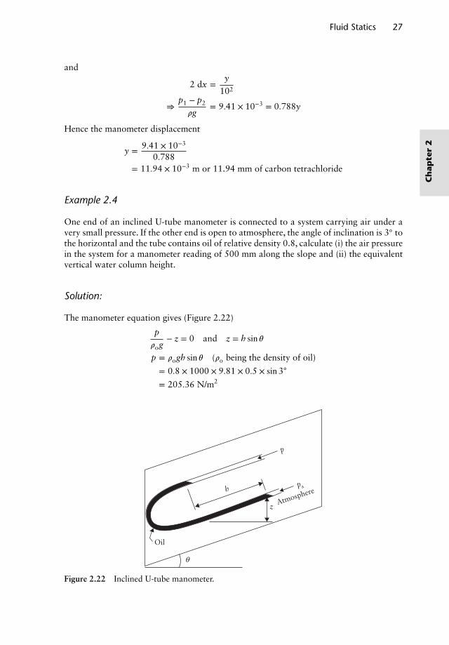
Example 2.4
One end of an inclined U-tube manometer is connected to a system carrying air under avery small pressure. If the other end is open to atmosphere, the angle of inclination is 3◦ tothe horizontal and the tube contains oil of relative density 0.8, calculate (i) the air pressurein the system for a manometer reading of 500 mm along the slope and (ii) the equivalentvertical water column height.
Solution:
The manometer equation gives (Figure 2.22)
p𝜌og
− z = 0 and z = h sin 𝜃
p = 𝜌ogh sin 𝜃 (𝜌o being the density of oil)
= 0.8 × 1000 × 9.81 × 0.5 × sin 3◦
= 205.36 N/m2
p
pah
z
Oil
Atmosphere
θ
Figure 2.22 Inclined U-tube manometer.
Ch
apte
r2
28 Civil Engineering Hydraulics
If h′ is the equivalent water column height and 𝜌 the density of water, we can write
p = 𝜌gh′ = 𝜌ogh sin 𝜃
⇒ h′ =(𝜌o
𝜌
)h sin 𝜃
= sh sin 𝜃= 0.8 × 0.5 × sin 3◦
= 2.09 × 10⁻² m
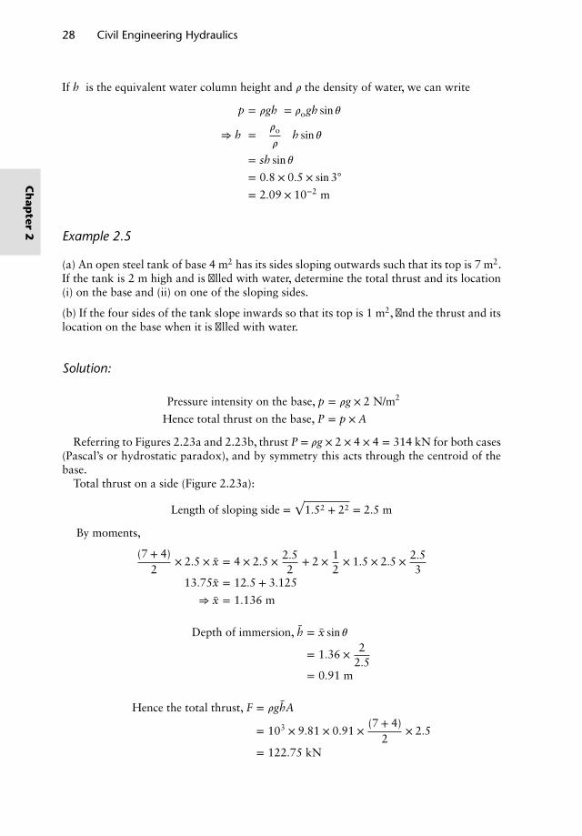
Example 2.5
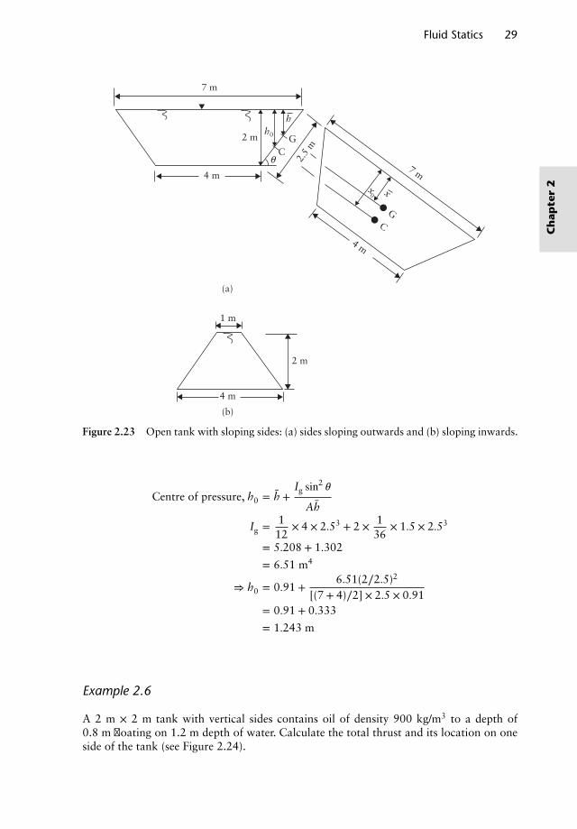
(a) An open steel tank of base 4 m2 has its sides sloping outwards such that its top is 7 m2.If the tank is 2 m high and is filled with water, determine the total thrust and its location(i) on the base and (ii) on one of the sloping sides.
(b) If the four sides of the tank slope inwards so that its top is 1 m2, find the thrust and itslocation on the base when it is filled with water.
Solution:
Pressure intensity on the base, p = 𝜌g × 2 N/m2
Hence total thrust on the base, P = p × A
Referring to Figures 2.23a and 2.23b, thrust P = 𝜌g × 2 × 4 × 4 = 314 kN for both cases(Pascal’s or hydrostatic paradox), and by symmetry this acts through the centroid of thebase.
Total thrust on a side (Figure 2.23a):
Length of sloping side =√
1.52 + 22 = 2.5 m
By moments,
(7 + 4)2
× 2.5 × x = 4 × 2.5 × 2.52
+ 2 × 12× 1.5 × 2.5 × 2.5
313.75x = 12.5 + 3.125
⇒ x = 1.136 m
Depth of immersion, h = x sin 𝜃
= 1.36 × 22.5
= 0.91 m
Hence the total thrust, F = 𝜌ghA
= 103 × 9.81 × 0.91 × (7 + 4)2
× 2.5
= 122.75 kN
Ch
apter
2
Fluid Statics 29
7 m
4 m
(a)
1 m
2 m
4 m
(b)
2 m G
7 m
4 m
GC
2.5
mCθ
h0
h
xx0
Figure 2.23 Open tank with sloping sides: (a) sides sloping outwards and (b) sloping inwards.
Centre of pressure, h0 = h +Ig sin
2𝜃
Ah
Ig = 112
× 4 × 2.53 + 2 × 136
× 1.5 × 2.53
= 5.208 + 1.302
= 6.51 m4
⇒ h0 = 0.91 +6.51(2∕2.5)2
[(7 + 4)∕2] × 2.5 × 0.91= 0.91 + 0.333
= 1.243 m
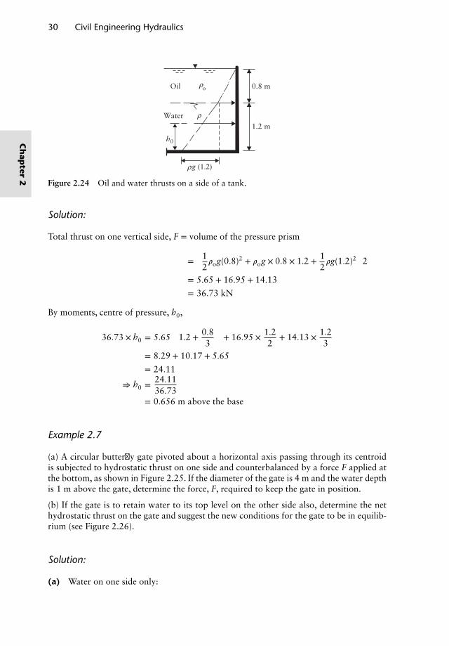
Example 2.6
A 2 m × 2 m tank with vertical sides contains oil of density 900 kg/m3 to a depth of0.8 m floating on 1.2 m depth of water. Calculate the total thrust and its location on oneside of the tank (see Figure 2.24).
Ch
apte
r2
30 Civil Engineering Hydraulics
Oil ρ
ρ
g (1.2)
1.2 m
0.8 m
Water
o
h0
ρ
Figure 2.24 Oil and water thrusts on a side of a tank.
Solution:
Total thrust on one vertical side, F = volume of the pressure prism
=[
12𝜌og(0.8)2 + 𝜌og × 0.8 × 1.2 + 1
2𝜌g(1.2)2
]2
= 5.65 + 16.95 + 14.13
= 36.73 kN
By moments, centre of pressure, h0,
36.73 × h0 = 5.65(
1.2 + 0.83
)+ 16.95 × 1.2
2+ 14.13 × 1.2
3= 8.29 + 10.17 + 5.65
= 24.11
⇒ h0 = 24.1136.73
= 0.656 m above the base
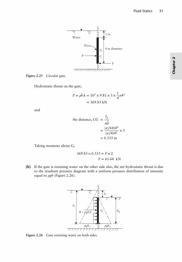
Example 2.7
(a) A circular butterfly gate pivoted about a horizontal axis passing through its centroidis subjected to hydrostatic thrust on one side and counterbalanced by a force F applied atthe bottom, as shown in Figure 2.25. If the diameter of the gate is 4 m and the water depthis 1 m above the gate, determine the force, F, required to keep the gate in position.
(b) If the gate is to retain water to its top level on the other side also, determine the nethydrostatic thrust on the gate and suggest the new conditions for the gate to be in equilib-rium (see Figure 2.26).
Solution:
(a) Water on one side only:
Ch
apter
2
Fluid Statics 31
Water
Pivot
G
C
1 m
4 m diameter
F
P
Figure 2.25 Circular gate.
Hydrostatic thrust on the gate,
P = 𝜌hA = 103 × 9.81 × 3 × 14𝜋42
= 369.83 kN
and
the distance, CG =Ig
Ah
=(𝜋∕64)44
(𝜋∕4)42× 3
= 0.333 m
Taking moments about G,
369.83 × 0.333 = F × 2
F = 61.64 kN
(b) If the gate is retaining water on the other side also, the net hydrostatic thrust is dueto the resultant pressure diagram with a uniform pressure distribution of intensityequal to 𝜌gh (Figure 2.26).
h
ρgh2ρgh1
R = ρghA h2
h1
G
Figure 2.26 Gate retaining water on both sides.
Ch
apte
r2
32 Civil Engineering Hydraulics
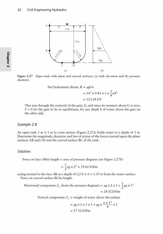
3 mA
B
DC
(b)(a)
2 g
3 g
3 m
r = 1 m
r = 1
m
ρ
ρ
Figure 2.27 Open tank with plane and curved surfaces: (a) tank elevation and (b) pressurediameter.
Net hydrostatic thrust, R = 𝜌ghA
= 103 × 9.81 × 1 × 14𝜋42
= 123.28 kN
This acts through the centroid of the gate, G, and since its moment about G is zero,F = 0 for the gate to be in equilibrium, for any depth h of water above the gate onthe other side.
Example 2.8
An open tank 3 m × 1 m in cross section (Figure 2.27a) holds water to a depth of 3 m.Determine the magnitude, direction and line of action of the forces exerted upon the planesurfaces AB and CD and the curved surface BC of the tank.
Solution:
Force on face AB/m length = area of pressure diagram (see Figure 2.27b)
= 12𝜌g × 22 = 19.62 kN/m
acting normal to the face AB at a depth of (2∕3) × 2 = 1.33 m from the water surface.Force on curved surface BC/m length:
Horizontal component,Fx (from the pressure diagram) = 𝜌g × 2 × 1 + 12𝜌g × 12
= 24.52 kN/m
Vertical component, Fy = weight of water above the surface
= 𝜌g × 2 × 1 × 1 + 𝜌g × 𝜋 × 12
4× 1
= 27.32 kN/m
Ch
apter
2
Fluid Statics 33
Resultant thrust, F =√
24.522 + 27.322
= 36.71 kN/m
acting at an angle 𝛼 = tan−1(27.32∕24.52) = 48◦5′ to the horizontal and passing throughthe centre of curvature of the surface BC.
Force on surface CD/m length:
Uniform pressure intensity on CD = 𝜌g × 3 N/m2
Total thrust on CD = uniform pressure × area
= 𝜌g × 3 × 1 × 1
= 29.43 kN/m
acting vertically downwards (normal to CD) through the mid-point of the surface CD.
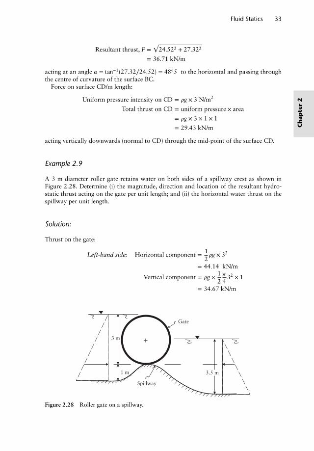
Example 2.9
A 3 m diameter roller gate retains water on both sides of a spillway crest as shown inFigure 2.28. Determine (i) the magnitude, direction and location of the resultant hydro-static thrust acting on the gate per unit length; and (ii) the horizontal water thrust on thespillway per unit length.
Solution:
Thrust on the gate:
Left-hand side: Horizontal component = 12𝜌g × 32
= 44.14 kN/m
Vertical component = 𝜌g × 12𝜋
432 × 1
= 34.67 kN/m
+
Gate
Spillway
1 m 3.5 m
3 m
Figure 2.28 Roller gate on a spillway.
Ch
apte
r2
34 Civil Engineering Hydraulics
Right-hand side: Horizontal component = 12𝜌g(1.5)2
= 11.03 kN/m
Vertical component = 𝜌g × 14𝜋
432 × 1
= 17.34 kN/m
Net horizontal component on the gate (left to right) = 44.14 − 11.03
= 33.11 kN/m
and
net vertical component (upwards) = 34.67 + 17.34
= 50.01 kN/m
Resultant hydrostatic thrust on the gate =√
(33.11)2 + (50.01)2
= 60 kN/m
acting at an angle 𝛼 = tan−1 (33.11∕50.01) = 33◦30′ to the vertical and passes through thecentre of the gate (normal to the surface).
Depth of centre of pressure = r + r cos 𝛼= 1.5 (1 + cos33◦30′)
= 2.75 m below the free surface of the left-hand side
Horizontal thrust on the spillway:From pressure diagrams (see Figure 2.28),
thrust from left-hand side = 12
(𝜌g × 3 + 𝜌g × 4) × 1
= 34.33 kN/m
and
thrust from right-hand side = 12
(𝜌g × 1.5 + 𝜌g × 3.5) × 2
= 49.05 kN/m
Resultant thrust (horizontal) on the spillway = 49.05 − 34.33
= 14.72 kN/m towards left
Example 2.10
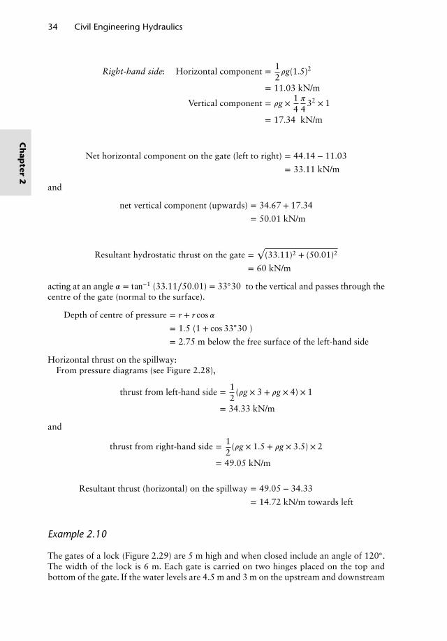
The gates of a lock (Figure 2.29) are 5 m high and when closed include an angle of 120◦.The width of the lock is 6 m. Each gate is carried on two hinges placed on the top andbottom of the gate. If the water levels are 4.5 m and 3 m on the upstream and downstream
Ch
apter
2
Fluid Statics 35
a
m5m6
3 m4.5 m
Rt sin 30°
Rb sin 30°
F1/2F2/2
A
(b)(a)
C
B
T
DR 1 F
120°
a
Figure 2.29 Lock gates: (a) plan view and (b) section a–a.
sides, respectively, determine the magnitudes of the forces on the hinges due to waterpressure.
Solution:
Forces on any one gate (say, AB) are as follows: F is the resultant water thrust; T, the thrustof gate; BC, normal to contact surface; andR, the resultant of hinge forces. Since these threeforces keep the gate in equilibrium, they should meet at a point D (Figure 2.29a).
Resolution of forces along AB and normal to AB gives (ABD = BAD = 30◦)
T cos30◦ = R cos 30◦ or T = R (i)
and
F = R sin 30◦ + T sin 30◦ or F = R (ii)
Length of the gate = 3∕ sin60◦ = 3.464 mThe resultant water thrusts on either side of the gate, F = F1 − F2:
F1 = 12𝜌g(4.5)2 × 3.464
= 344 kN acting at 4.5∕3 = 1.5 m from the base
and F2 = 12𝜌g × 32 × 3.464
= 153 kN acting at 3∕3 = 1 m from the base
Resultant water thrust, F = 344 − 153
= 191 kN = R (from Equation (ii))
Total hinge reaction, R = Rt + Rb (sum of top and bottom hinge forces) (iii)
From Equation (ii),
F2= R sin 30◦
or
F1 − F2
2= Rt sin 30◦ + Rb sin30◦ (iv)
Ch
apte
r2
36 Civil Engineering Hydraulics
Taking moments about the bottom hinge (Figure 2.29b),
3442
× 1.5 − 1532
× 1 = Rt sin 30◦ × 5
⇒ Rt = 72.6 kN
and hence from Equation (iii),
Rb = 191 − 72.6
= 118.4 kN
Example 2.11
A rectangular block of wood floats in water with 50 mm projecting above the water sur-face. When placed in glycerine of relative density 1.35, the block projects 75 mm abovethe surface of glycerine. Determine the relative density of the wood.
Solution:
Weight of wooden block,W = upthrust in water = upthrust in glycerine
= weight of fluid displaced
W = 𝜌wgAh = 𝜌gA(h − 50 × 10−3) = 𝜌GgA(h − 75 × 10−3)
𝜌, 𝜌w and 𝜌G being the densities of water, wood and glycerine, respectively; A the cross-sectional area of the block; and h its height.
The relative density of glycerine,𝜌G
𝜌= h − 50 × 10−3
h − 75 × 10−3= 1.35
⇒ h = 146.43 × 10⁻³ m or 146.43 mm
Hence the relative density of wood,𝜌w
𝜌= 146.43 − 50
146.43= 0.658
Example 2.12
(a) A ship of 50 MN displacement has a weight of 100 kN moved 10 m across the deckcausing a heel angle of 5◦. Find the metacentric height of the ship.
(b) A homogeneous circular cylinder of radius R and height H is to float stably in a liquid.Show that R must not be less than
√2r(1 − r)H in order to float with its axis vertical,
where r is the ratio of relative densities of the cylinder and the liquid. Hence establish thecondition for R∕H to be minimum.
Solution:
Referring to Figure 2.30a,
Ch
apter
2
Fluid Statics 37
Radius, R
H
MM
B
O
GG
G′
B′B
h Liquid
rd = s2
Fb = W = 50 MN(a)
θ
(b)
10 m
rd = s1
100 kN+
+
W
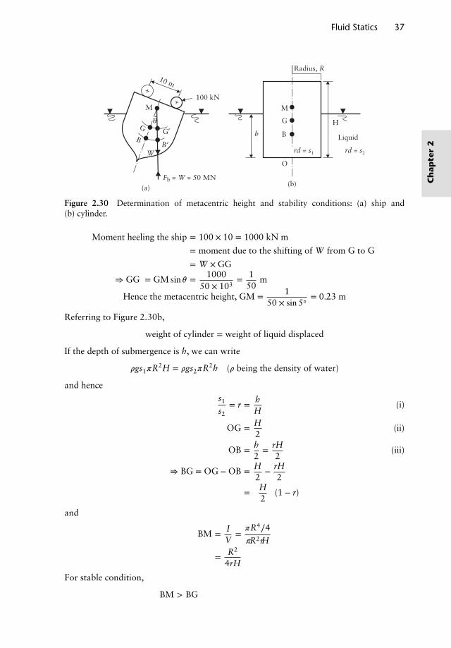
Figure 2.30 Determination of metacentric height and stability conditions: (a) ship and(b) cylinder.
Moment heeling the ship = 100 × 10 = 1000 kN m
= moment due to the shifting of W from G to G′
= W × GG′
⇒ GG′ = GM sin 𝜃 = 100050 × 103
= 150
m
Hence the metacentric height, GM = 150 × sin 5◦
= 0.23 m
Referring to Figure 2.30b,
weight of cylinder = weight of liquid displaced
If the depth of submergence is h, we can write
𝜌gs1𝜋R2H = 𝜌gs2𝜋R
2h (𝜌 being the density of water)
and hences1
s2= r = h
H(i)
OG = H2
(ii)
OB = h2= rH
2(iii)
⇒ BG = OG − OB = H2
− rH2
=(H
2
)(1 − r)
and
BM = IV
=𝜋R4∕4𝜋R2rH
= R2
4rH
For stable condition,
BM > BG
Ch
apte
r2
38 Civil Engineering Hydraulics
10 m
1 m
2 m
ax
ax = 3 m/s2
θ
θ
g(2 + h)
(b)(a)
2 g
B
A
10 m
h
2 m
gh
C
D
ρ
ρ
ρ
Figure 2.31 Oil tanker subjected to accelerations: (a) half full and (b) full.
R2
4rH>
(H2
)(1 − r) or R2
H2> 2r(1 − r)
⇒RH>
√2r(1 − r)
and hence
R >√
2r(1 − r)H
For limiting value of R∕H, r(1 − r) is to be minimum or
d [r(1 − r)] = 0
⇒ 1 − 2r = 0 and hence r = 12
Example 2.13
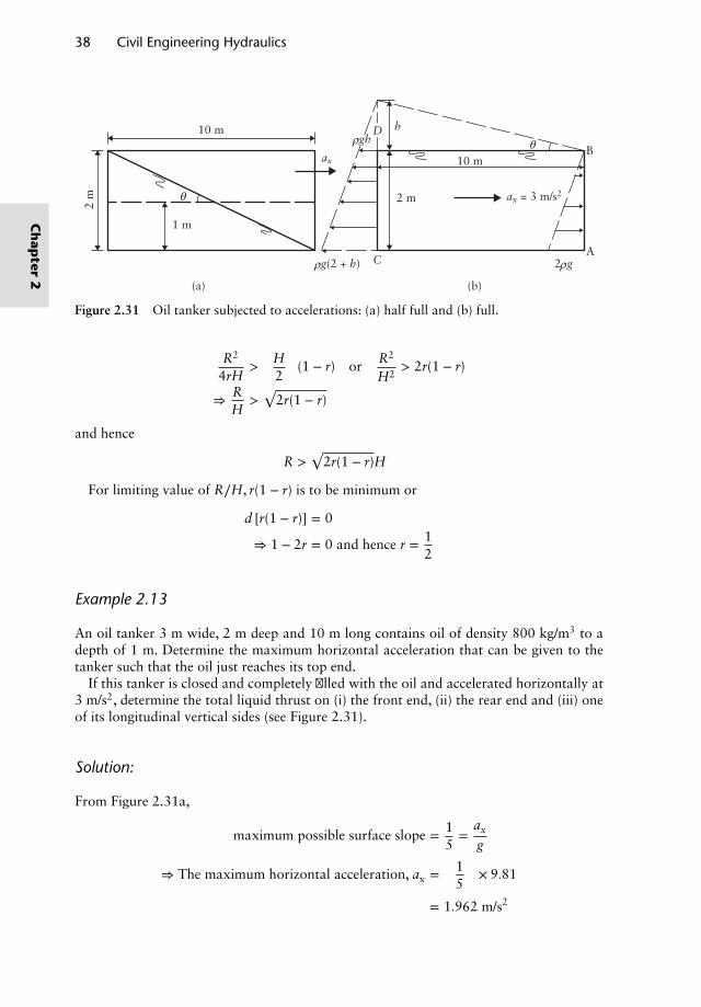
An oil tanker 3 m wide, 2 m deep and 10 m long contains oil of density 800 kg/m3 to adepth of 1 m. Determine the maximum horizontal acceleration that can be given to thetanker such that the oil just reaches its top end.
If this tanker is closed and completely filled with the oil and accelerated horizontally at3 m/s2, determine the total liquid thrust on (i) the front end, (ii) the rear end and (iii) oneof its longitudinal vertical sides (see Figure 2.31).
Solution:
From Figure 2.31a,
maximum possible surface slope = 15=
ax
g
⇒ The maximum horizontal acceleration, ax =(
15
)× 9.81
= 1.962 m/s2
Ch
apter
2
Fluid Statics 39
When the tanker is completely filled and closed, there will be pressure built up at therear-end equivalent to the virtual oil column (h) that would assume a slope of ax∕g (Figure2.31b).
(i) Total thrust on front end AB = 12𝜌g × 22 × 3 = 58.86 kN
(ii) Total thrust on rear end CD:Virtual rise of oil level at rear end,
h = 10 × tan 𝜃 = 10 ×ax
g= 10 × 3
9.81= 3.06 m
Total thrust on CD =𝜌g(3.06) + 𝜌g(2 + 3.06)
2× 2 × 3
= 239 kN
(iii) Total thrust on side ABCD = volume of the pressure prism
= 12𝜌g × 22 × 10 + 1
2𝜌g × 3.06 × 10 × 2
= 12𝜌g(2 + 3.06) × 2 × 10
= 496 kN
Example 2.14
A vertical hoist carries a square tank of 2 m × 2 m containing water to the top of aconstruction scaffold with a varying speed of 2 m/s. If the water depth is 2 m, calculatethe total hydrostatic thrust on the bottom of the tank.
If this tank of water is lowered with an acceleration equal to that of gravity, what arethe thrusts on the floor and sides of the tank?
Solution:
Vertical upward acceleration, ay = 2 m/s2
Pressure intensity at a depth h = 𝜌gh(
1 +ay
g
)
= 𝜌gh(
1 + 29.81
)= 1.204 × gh kN/m2
Total hydrostatic thrust on the floor = intensity × area
= 1.204 × 9.81 × 2 × 2 × 2
= 94.5 kN
Downward acceleration = −9.81 m/s2
Pressure intensity at a depth h = 𝜌gh(
1 − 9.819.81
)= 0
Therefore, there exists no hydrostatic thrust on the floor, nor on the sides.
Ch
apte
r2
40 Civil Engineering Hydraulics
150 mm diameter
375 mm
r
375 mm
150 mm
1287
mm
(a)
(b)
320 mm
Figure 2.32 Rotating cylinder: (a) 𝜔 = 33.5 rad/s and (b) 𝜔 = 67.0 rad/s.
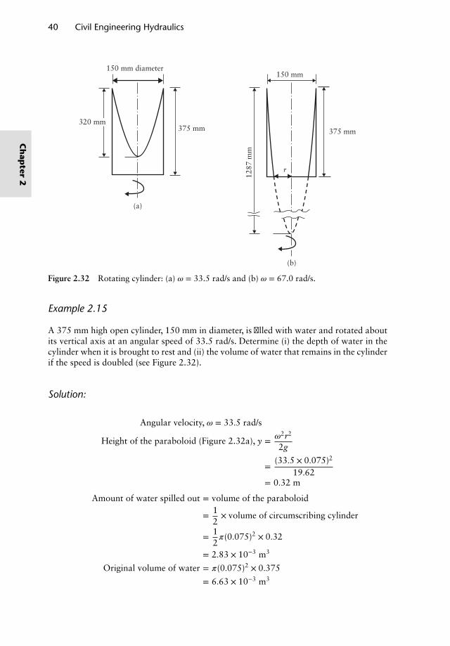
Example 2.15
A 375 mm high open cylinder, 150 mm in diameter, is filled with water and rotated aboutits vertical axis at an angular speed of 33.5 rad/s. Determine (i) the depth of water in thecylinder when it is brought to rest and (ii) the volume of water that remains in the cylinderif the speed is doubled (see Figure 2.32).
Solution:
Angular velocity, 𝜔 = 33.5 rad/s
Height of the paraboloid (Figure 2.32a), y = 𝜔2r2
2g
= (33.5 × 0.075)2
19.62= 0.32 m
Amount of water spilled out = volume of the paraboloid
= 12× volume of circumscribing cylinder
= 12𝜋(0.075)2 × 0.32
= 2.83 × 10⁻³ m3
Original volume of water = 𝜋(0.075)2 × 0.375
= 6.63 × 10⁻³ m3
Ch
apter
2
Fluid Statics 41
Remaining volume of water = (6.63 − 2.83) × 10−3
= 3.8 × 10⁻³ m3
Hence the depth of water at rest = 3.8 × 10⁻³
𝜋(0.075)2
= 0.215 m
If the speed is doubled, 𝜔 = 67 rad/s.
Height of paraboloid = (67 × 0.075)2
2g= 1.287 m
The free surface in the vessel assumes the shape as shown in Figure 2.32b, and we canwrite
1.287 − 0.375 = 𝜔2r2
2g
r =√
2g × 0.912672
= 0.063 m
Therefore, the volume of water spilled out = 12𝜋(0.075)2
×1.287 − 12𝜋(0.063)2 × 0.912
= 5.684 × 10⁻³m3
Hence the volume of water left = (6.63 − 5.684) × 10−3
= 0.946 × 10⁻³ m3
Reference and recommended reading
Zipparro, V. J. and Hasen, H. (1993) Davis’ Handbook of Applied Hydraulics, 4th edn,McGraw-Hill, New York.
Problems
1. (a) A large storage tank contains a salt solution of variable density given by 𝜌 = 1050 +kh in kilograms per cubic metre, where k = 50 kg∕m4, at a depth h (in metres) belowthe free surface. Calculate the pressure intensity at the bottom of the tank holding5 m of the solution.
(b) A Bourdon-type pressure gauge is connected to a hydraulic cylinder activated by apiston of 20 mm diameter. If the gauge balances a total mass of 10 kg placed on thepiston, determine the gauge reading (in metres) of water.
2. A closed cylindrical tank 4 m high is partly filled with oil of density 800 kg/m3 to adepth of 3 m. The remaining space is filled with air under pressure. A U-tube containingmercury (of relative density 13.6) is used to measure the air pressure, with one end open toatmosphere. Find the gauge pressure at the base of the tank when the mercury deflection
Ch
apte
r2
42 Civil Engineering Hydraulics
in the open limb of the U-tube is (i) 100 mm above and (ii) 100 mm below the level inthe other limb.
3. A manometer consists of a glass tube, inclined at 30◦ to the horizontal, connected toa metal cylinder standing upright. The upper end of the cylinder is connected to a gassupply under pressure. Find the pressure (in millimetres) of water when the manometerfluid of relative density 0.8 reads a deflection of 80 mm along the tube. Take the ratio, r,of the diameters of the cylinder and the tube as 64. What value of r would you suggest sothat the error due to disregarding the change in level in the cylinder will not exceed 0.2%?
4. In order to measure the pressure difference between two points in a pipeline carryingwater, an inverted U-tube is connected to the points, and air under atmospheric pressureis entrapped in the upper portion of the U-tube. If the manometer deflection is 0.8 m andthe downstream tapping is 0.5 m below the upstream point, find the pressure differencebetween the two points.
5. A high-pressure gas pipeline is connected to a macromanometer consisting of fourU-tubes in series with one end open to atmosphere, and a deflection of 500 mm ofmercury (of relative density 13.6) has been observed. If water is entrapped between themercury columns of the manometer and the relative density of the gas is 1.2 × 10⁻³,calculate the gas pressure in newtons per millimetre square, the centre line of the pipelinebeing at a height of 0.50 m above the top mercury level.
6. A dock gate is to be reinforced with three identical horizontal beams. If the water standsto depths of 5 m and 3 m on either side, find the positions of the beams, measured abovethe floor level, so that each beam will carry an equal load, and calculate the load oneach beam per unit length.
7. A storage tank of a sewage treatment plant is to discharge excess sewage into the seathrough a horizontal rectangular culvert 1 m deep and 1.3 m wide. The face of thedischarge end of the culvert is inclined at 40◦ to the vertical and the storage level iscontrolled by a flap gate weighing 4.5 kN, hinged at the top edge and just covering theopening. When the sea water stands to the hinge level, to what height above the top ofthe culvert will the sewage be stored before a discharge occurs? Take the density of thesewage as 1000 kg/m3 and of the sea water as 1025 kg/m3.
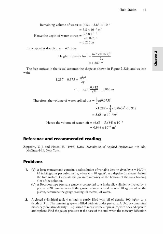
8. A radial gate, 2 m long, hinged about a horizontal axis closes the rectangular sluice ofa control dam by the application of a counterweight W (see Figure 2.33). Determine (i)the total hydrostatic thrust and its location on the gate when the storage depth is 4 mand (ii) for the gate to be stable, the counterweight W. Explain what will happen if thestorage increases beyond 4 m.
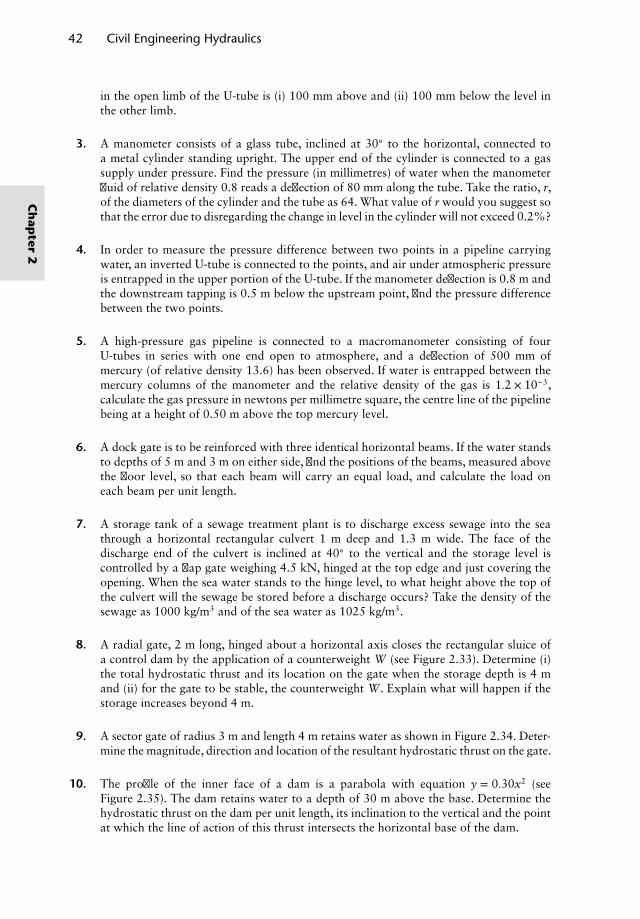
9. A sector gate of radius 3 m and length 4 m retains water as shown in Figure 2.34. Deter-mine the magnitude, direction and location of the resultant hydrostatic thrust on the gate.
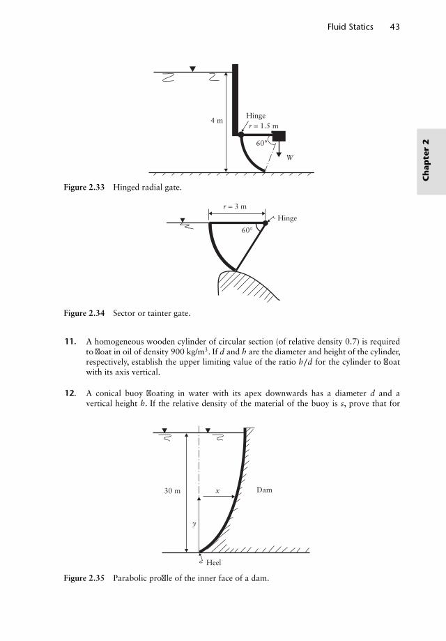
10. The profile of the inner face of a dam is a parabola with equation y = 0.30x2 (seeFigure 2.35). The dam retains water to a depth of 30 m above the base. Determine thehydrostatic thrust on the dam per unit length, its inclination to the vertical and the pointat which the line of action of this thrust intersects the horizontal base of the dam.
Ch
apter
2
Fluid Statics 43
Hinge
60°
W
r = 1.5 m4 m
Figure 2.33 Hinged radial gate.
Hinge
r = 3 m
60°
Figure 2.34 Sector or tainter gate.
11. A homogeneous wooden cylinder of circular section (of relative density 0.7) is requiredto float in oil of density 900 kg/m3. If d and h are the diameter and height of the cylinder,respectively, establish the upper limiting value of the ratio h∕d for the cylinder to floatwith its axis vertical.
12. A conical buoy floating in water with its apex downwards has a diameter d and avertical height h. If the relative density of the material of the buoy is s, prove that for
30 m Dam
Heel
x
y
Figure 2.35 Parabolic profile of the inner face of a dam.
Ch
apte
r2
44 Civil Engineering Hydraulics
0.6 m0.3 m
0.25 m
0.3 m
(b)(a)
h h
0.3 m
0.25 m
10 m
Figure 2.36 Floating platform: (a) single beam and (b) platform.
stable equilibrium,
hd<
12
√s1∕3
1 − s1∕3
13. A cyclindrical buoy weighing 20 kN is to float in sea water whose density is 1020 kg/m3.The buoy has a diameter of 2 m and height of 2.5 m. Prove that it is unstable.
If the buoy is anchored with a chain attached to the centre of its base, find the tensionin the chain to keep the buoy in vertical position.
14. A floating platform for offshore drilling purposes is in the form of a square floorsupported by four vertical cylinders at the corners. Determine the location of thecentroid of the assembly in terms of the side L of the floor and the depth of submergenceh of the cylinders so as to float in neutral equilibrium under a uniformly distributedloading condition.
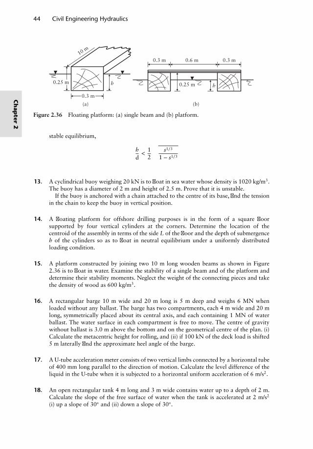
15. A platform constructed by joining two 10 m long wooden beams as shown in Figure2.36 is to float in water. Examine the stability of a single beam and of the platform anddetermine their stability moments. Neglect the weight of the connecting pieces and takethe density of wood as 600 kg/m3.
16. A rectangular barge 10 m wide and 20 m long is 5 m deep and weighs 6 MN whenloaded without any ballast. The barge has two compartments, each 4 m wide and 20 mlong, symmetrically placed about its central axis, and each containing 1 MN of waterballast. The water surface in each compartment is free to move. The centre of gravitywithout ballast is 3.0 m above the bottom and on the geometrical centre of the plan. (i)Calculate the metacentric height for rolling, and (ii) if 100 kN of the deck load is shifted5 m laterally find the approximate heel angle of the barge.
17. A U-tube acceleration meter consists of two vertical limbs connected by a horizontal tubeof 400 mm long parallel to the direction of motion. Calculate the level difference of theliquid in the U-tube when it is subjected to a horizontal uniform acceleration of 6 m/s2.
18. An open rectangular tank 4 m long and 3 m wide contains water up to a depth of 2 m.Calculate the slope of the free surface of water when the tank is accelerated at 2 m/s2
(i) up a slope of 30◦ and (ii) down a slope of 30◦.
Ch
apter
2
Fluid Statics 45
19. Prove that in the forced vortex motion (fluids subjected to rotation externally) of aliquid, the rate of increase of the pressure p with respect to the radius r at a point inliquid is given by dp/dr = 𝜌𝜔2r, in which 𝜔 is the angular velocity of the liquid and 𝜌 isits mass density. Hence calculate the thrust of the liquid on the top of a closed verticalcylinder of 450 mm diameter, completely filled with water under a pressure of 10 N/cm2,when the cylinder rotates about its axis at 240 rpm.
Ch
apte
r2

Chapter 3Fluid Flow Conceptsand Measurements
3.1 Kinematics of fluids
The kinematics of fluids deals with space–time relationships for fluids in motion. In theLagrangian method of describing the fluid motion, one is concerned to trace the paths ofthe individual fluid particles (elements) and to find their velocities, pressures and so onwith the passage of time. The coordinates of a particle A(x, y, z) at any time t (Figure 3.1a)are dependent on its initial coordinates (a, b, c) at the instant t0 and can be written asfunctions of a, b, c and t; in other words,
x = 𝜙1(a, b, c, t)
y = 𝜙2(a, b, c, t)
z = 𝜙3(a, b, c, t)
The path traced by the particles over a period of time is known as the pathline. Due tothe diffusivity phenomena of fluids and their flows, it is difficult to describe the motionof individual particles of a flow field with time. More appropriate for describing the fluidmotion is to know the flow characteristics such as velocity and pressure of a particle orgroup of particles at a chosen point in the flow field at any particular time; such a descrip-tion of fluid flow is known as the Eulerian method.
In any flow field, velocity is the most important characteristic to be identified at anypoint. The velocity vector at a point in the flow field is a function of s and t and can beresolved into u, v and w components, representing velocities in the x-, y- and z-directions,respectively; these components are functions of x, y, z and t and written as (Figure 3.1b)
u = f1(x, y, z, t)
v = f2(x, y, z, t)
w = f3(x, y, z, t)
defining the vector V at each point in the space at any instant t. A continuous curve tracedtangentially to the velocity vector at each point in the flow field is known as the streamline.
Nalluri & Featherstone’s Civil Engineering Hydraulics: Essential Theory with Worked Examples,Sixth Edition. Martin Marriott.© 2016 John Wiley & Sons, Ltd. Published 2016 by John Wiley & Sons, Ltd.Companion Website: www.wiley.com/go/Marriott
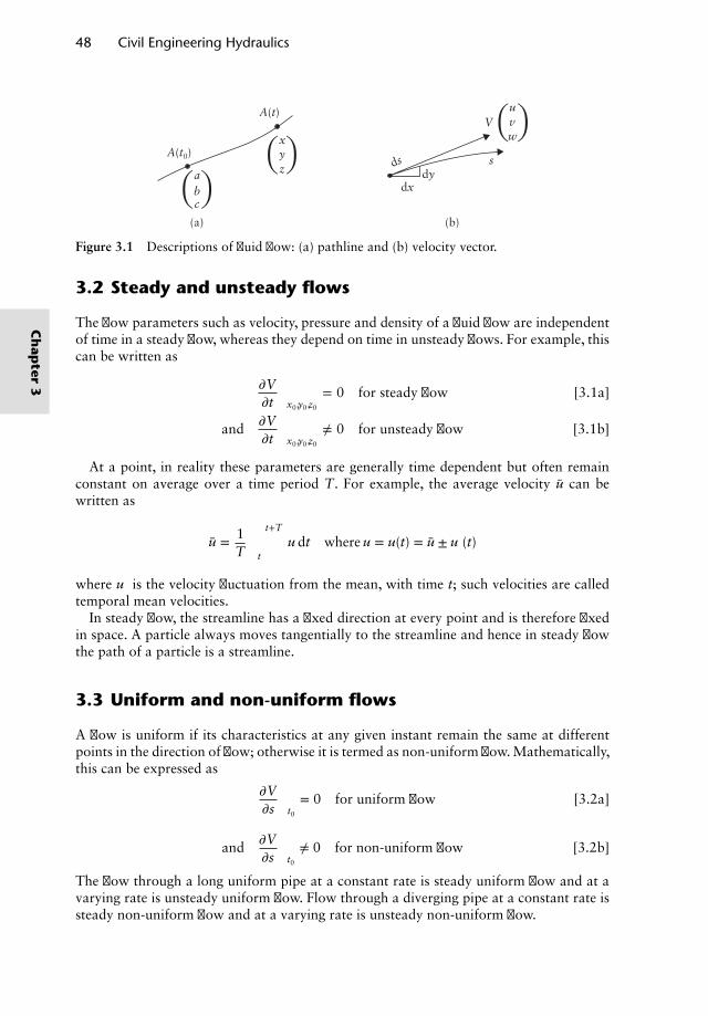
48 Civil Engineering Hydraulics
A(t0)
A(t)
x
zy
u
w
s
V
dydx
(b)(a)
ds
v
a
cb
Figure 3.1 Descriptions of fluid flow: (a) pathline and (b) velocity vector.
3.2 Steady and unsteady flows
The flow parameters such as velocity, pressure and density of a fluid flow are independentof time in a steady flow, whereas they depend on time in unsteady flows. For example, thiscan be written as (
𝜕V𝜕t
)x0,y0,z0
= 0 for steady flow [3.1a]
and(𝜕V𝜕t
)x0,y0,z0
≠ 0 for unsteady flow [3.1b]
At a point, in reality these parameters are generally time dependent but often remainconstant on average over a time period T. For example, the average velocity u can bewritten as
u = 1T ∫
t+T
tu dt where u = u(t) = u ± u′(t)
where u′ is the velocity fluctuation from the mean, with time t; such velocities are calledtemporal mean velocities.
In steady flow, the streamline has a fixed direction at every point and is therefore fixedin space. A particle always moves tangentially to the streamline and hence in steady flowthe path of a particle is a streamline.
3.3 Uniform and non-uniform flows
A flow is uniform if its characteristics at any given instant remain the same at differentpoints in the direction of flow; otherwise it is termed as non-uniform flow. Mathematically,this can be expressed as (
𝜕V𝜕s
)t0
= 0 for uniform flow [3.2a]
and(𝜕V𝜕s
)t0
≠ 0 for non-uniform flow [3.2b]
The flow through a long uniform pipe at a constant rate is steady uniform flow and at avarying rate is unsteady uniform flow. Flow through a diverging pipe at a constant rate issteady non-uniform flow and at a varying rate is unsteady non-uniform flow.
Ch
apter
3
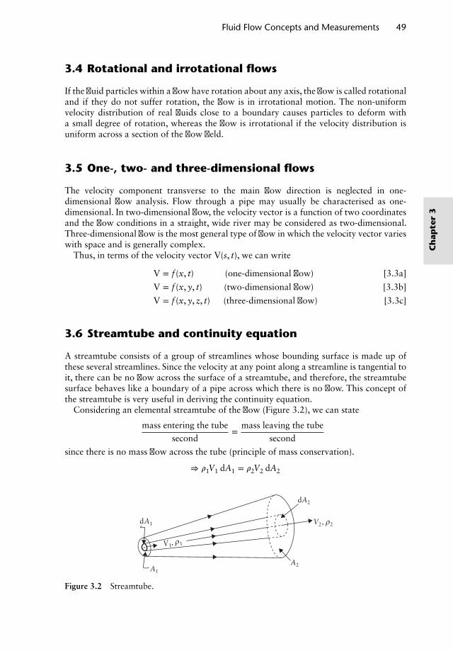
Fluid Flow Concepts and Measurements 49
3.4 Rotational and irrotational flows
If the fluid particles within a flow have rotation about any axis, the flow is called rotationaland if they do not suffer rotation, the flow is in irrotational motion. The non-uniformvelocity distribution of real fluids close to a boundary causes particles to deform witha small degree of rotation, whereas the flow is irrotational if the velocity distribution isuniform across a section of the flow field.
3.5 One-, two- and three-dimensional flows
The velocity component transverse to the main flow direction is neglected in one-dimensional flow analysis. Flow through a pipe may usually be characterised as one-dimensional. In two-dimensional flow, the velocity vector is a function of two coordinatesand the flow conditions in a straight, wide river may be considered as two-dimensional.Three-dimensional flow is the most general type of flow in which the velocity vector varieswith space and is generally complex.
Thus, in terms of the velocity vector V(s, t), we can write
V = f (x, t) (one-dimensional flow) [3.3a]
V = f (x, y, t) (two-dimensional flow) [3.3b]
V = f (x, y, z, t) (three-dimensional flow) [3.3c]
3.6 Streamtube and continuity equation
A streamtube consists of a group of streamlines whose bounding surface is made up ofthese several streamlines. Since the velocity at any point along a streamline is tangential toit, there can be no flow across the surface of a streamtube, and therefore, the streamtubesurface behaves like a boundary of a pipe across which there is no flow. This concept ofthe streamtube is very useful in deriving the continuity equation.
Considering an elemental streamtube of the flow (Figure 3.2), we can state
mass entering the tube
second=
mass leaving the tube
second
since there is no mass flow across the tube (principle of mass conservation).
⇒ 𝜌1V1 dA1 = 𝜌2V2 dA2
dA1
A1
A2
V2, ρ2
V1, ρ1
dA2
Figure 3.2 Streamtube.
Ch
apte
r3
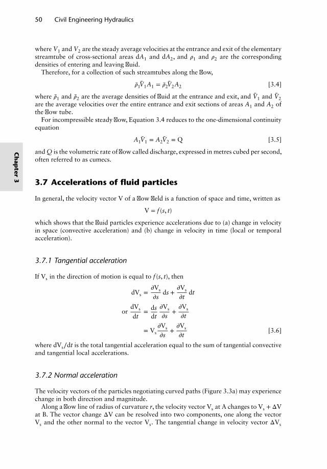
50 Civil Engineering Hydraulics
where V1 and V2 are the steady average velocities at the entrance and exit of the elementarystreamtube of cross-sectional areas dA1 and dA2, and 𝜌1 and 𝜌2 are the correspondingdensities of entering and leaving fluid.
Therefore, for a collection of such streamtubes along the flow,
��1V1A1 = ��2V2A2 [3.4]
where ��1 and ��2 are the average densities of fluid at the entrance and exit, and V1 and V2are the average velocities over the entire entrance and exit sections of areas A1 and A2 ofthe flow tube.
For incompressible steady flow, Equation 3.4 reduces to the one-dimensional continuityequation
A1V1 = A2V2 = Q [3.5]
and Q is the volumetric rate of flow called discharge, expressed in metres cubed per second,often referred to as cumecs.
3.7 Accelerations of fluid particles
In general, the velocity vector V of a flow field is a function of space and time, written as
V = f (s, t)
which shows that the fluid particles experience accelerations due to (a) change in velocityin space (convective acceleration) and (b) change in velocity in time (local or temporalacceleration).
3.7.1 Tangential acceleration
If Vs in the direction of motion is equal to f (s, t), then
dVs =𝜕Vs
𝜕sds +
𝜕Vs
𝜕tdt
ordVs
dt= ds
dt
𝜕Vs
𝜕s+𝜕Vs
𝜕t
= Vs𝜕Vs
𝜕s+𝜕Vs
𝜕t[3.6]
where dVs∕dt is the total tangential acceleration equal to the sum of tangential convectiveand tangential local accelerations.
3.7.2 Normal acceleration
The velocity vectors of the particles negotiating curved paths (Figure 3.3a) may experiencechange in both direction and magnitude.
Along a flow line of radius of curvature r, the velocity vector Vs at A changes to Vs + ΔVat B. The vector change ΔV can be resolved into two components, one along the vectorVs and the other normal to the vector Vs. The tangential change in velocity vector ΔVs
Ch
apter
3
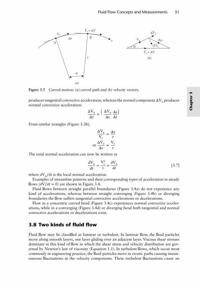
Fluid Flow Concepts and Measurements 51
AΔs
Vs
Vs
ΔVs
ΔV
Vs + ΔV
Vs + ΔV
Bs
α
(a)
(b)
ΔVnα
r
Figure 3.3 Curved motion: (a) curved path and (b) velocity vectors.
produces tangential convective acceleration, whereas the normal componentΔVn producesnormal convective acceleration:
ΔVn
Δt=(ΔVn
ΔsΔsΔt
)
From similar triangles (Figure 3.3b),
ΔVn
Vs= Δs
r
orΔVn
Δs=
Vs
r
The total normal acceleration can now be written as
dVn
dt=
V2s
r+𝜕Vn
𝜕t[3.7]
where 𝜕Vn∕𝜕t is the local normal acceleration.Examples of streamline patterns and their corresponding types of acceleration in steady
flows (𝜕V∕𝜕t = 0) are shown in Figure 3.4.Fluid flows between straight parallel boundaries (Figure 3.4a) do not experience any
kind of accelerations, whereas between straight converging (Figure 3.4b) or divergingboundaries the flow suffers tangential convective accelerations or decelerations.
Flow in a concentric curved bend (Figure 3.4c) experiences normal convective acceler-ations, while in a converging (Figure 3.4d) or diverging bend both tangential and normalconvective accelerations or decelerations exist.
3.8 Two kinds of fluid flow
Fluid flow may be classified as laminar or turbulent. In laminar flow, the fluid particlesmove along smooth layers, one layer gliding over an adjacent layer. Viscous shear stressesdominate in this kind of flow in which the shear stress and velocity distribution are gov-erned by Newton’s law of viscosity (Equation 1.1). In turbulent flows, which occur mostcommonly in engineering practice, the fluid particles move in erratic paths causing instan-taneous fluctuations in the velocity components. These turbulent fluctuations cause an
Ch
apte
r3
52 Civil Engineering Hydraulics
(b)(a)
(d)(c)
Figure 3.4 Streamline patterns and types of acceleration: (a) no accelerations exist; (b) tangen-tial convective accelerations; (c) normal convective accelerations; and (d) tangential and normalconvective accelerations.
exchange of momentum setting up additional shear stresses of large magnitudes. An equa-tion of the form similar to Newton’s law of viscosity (Equation 1.1) may be written forturbulent flow by replacing 𝜇 by 𝜂. The coefficient 𝜂, called the eddy viscosity, depends onthe fluid motion and the density.
The type of a flow is identified by the Reynolds number, Re = 𝜌VL∕𝜇, where 𝜌 and 𝜇 arethe density and viscosity of the fluid, V is the flow velocity and L is a characteristic lengthsuch as the pipe diameter (D) in the case of a pipe flow. Reynolds number represents theratio of inertial forces to the viscous forces that exist in the flow field and is dimensionless.
The flow through a pipe is always laminar if the corresponding Reynolds number (Re =𝜌VD∕𝜇) is less than 2000, and for all practical purposes the flow may be assumed to passthrough a transition to full turbulent flow in the range of Reynolds numbers from 2000to 4000.
3.9 Dynamics of fluid flow
The study of fluid dynamics deals with the forces responsible for fluid motion and theresulting accelerations. A fluid in motion experiences, in addition to gravity, pressureforces, viscous and turbulent shear resistances, boundary resistance and forces due to sur-face tension and compressibility effects of the fluid. The presence of such a complex systemof forces in real fluid flow problems makes the analysis very complicated.
However, a simplifying approach to the problem may be made by assuming the fluid tobe ideal or perfect (i.e. non-viscous or frictionless and incompressible). Water has a rela-tively low viscosity and is practically incompressible and is found to behave like an idealfluid. The study of ideal fluid motion is a valuable background information to encounterthe problems of civil engineering hydraulics.
3.10 Energy equation for an ideal fluid flow
Consider an elemental streamtube in motion along a streamline (Figure 3.5) of an idealfluid flow.
Ch
apter
3
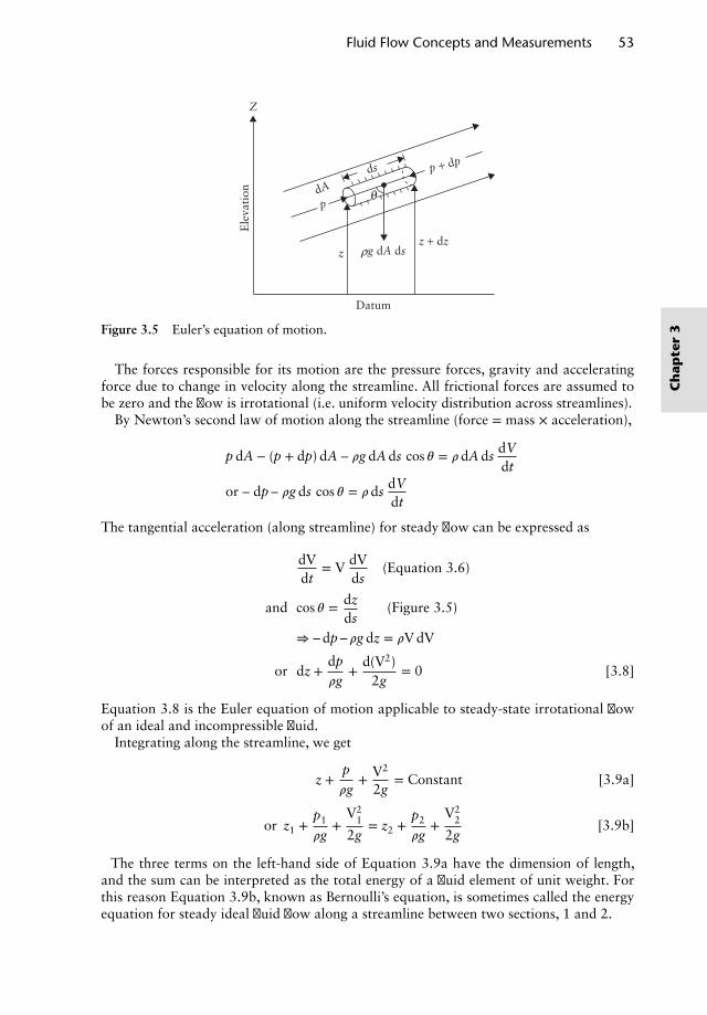
Fluid Flow Concepts and Measurements 53
Datum
z g dA dsz + dz
p + dp
p
ds
dAθ
Z
Ele
vati
onρ
Figure 3.5 Euler’s equation of motion.
The forces responsible for its motion are the pressure forces, gravity and acceleratingforce due to change in velocity along the streamline. All frictional forces are assumed tobe zero and the flow is irrotational (i.e. uniform velocity distribution across streamlines).
By Newton’s second law of motion along the streamline (force = mass × acceleration),
p dA − (p + dp) dA – 𝜌g dA ds cos 𝜃 = 𝜌dA dsdVdt
or – dp – 𝜌g ds cos 𝜃 = 𝜌dsdVdt
The tangential acceleration (along streamline) for steady flow can be expressed as
dVdt
= V dVds
(Equation 3.6)
and cos 𝜃 = dzds
(Figure 3.5)
⇒ – dp – 𝜌g dz = 𝜌V dV
or dz +dp𝜌g
+d(V2)
2g= 0 [3.8]
Equation 3.8 is the Euler equation of motion applicable to steady-state irrotational flowof an ideal and incompressible fluid.
Integrating along the streamline, we get
z +p𝜌g
+ V2
2g= Constant [3.9a]
or z1 +p1
𝜌g+
V21
2g= z2 +
p2
𝜌g+
V22
2g[3.9b]
The three terms on the left-hand side of Equation 3.9a have the dimension of length,and the sum can be interpreted as the total energy of a fluid element of unit weight. Forthis reason Equation 3.9b, known as Bernoulli’s equation, is sometimes called the energyequation for steady ideal fluid flow along a streamline between two sections, 1 and 2.
Ch
apte
r3
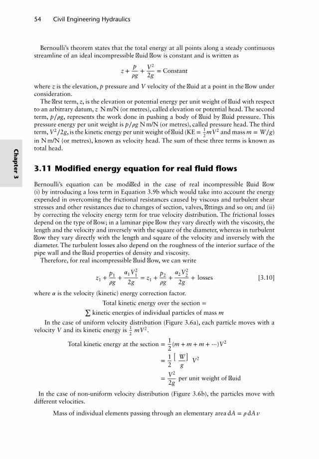
54 Civil Engineering Hydraulics
Bernoulli’s theorem states that the total energy at all points along a steady continuousstreamline of an ideal incompressible fluid flow is constant and is written as
z +p𝜌g
+ V2
2g= Constant
where z is the elevation, p pressure and V velocity of the fluid at a point in the flow underconsideration.
The first term, z, is the elevation or potential energy per unit weight of fluid with respectto an arbitrary datum, z N m/N (or metres), called elevation or potential head. The secondterm, p∕𝜌g, represents the work done in pushing a body of fluid by fluid pressure. Thispressure energy per unit weight is p∕𝜌g N m/N (or metres), called pressure head. The thirdterm, V2∕2g, is the kinetic energy per unit weight of fluid (KE= 1
2mV2 and mass m = W∕g)
in N m/N (or metres), known as velocity head. The sum of these three terms is known astotal head.
3.11 Modified energy equation for real fluid flows
Bernoulli’s equation can be modified in the case of real incompressible fluid flow(i) by introducing a loss term in Equation 3.9b which would take into account the energyexpended in overcoming the frictional resistances caused by viscous and turbulent shearstresses and other resistances due to changes of section, valves, fittings and so on; and (ii)by correcting the velocity energy term for true velocity distribution. The frictional lossesdepend on the type of flow; in a laminar pipe flow they vary directly with the viscosity, thelength and the velocity and inversely with the square of the diameter, whereas in turbulentflow they vary directly with the length and square of the velocity and inversely with thediameter. The turbulent losses also depend on the roughness of the interior surface of thepipe wall and the fluid properties of density and viscosity.
Therefore, for real incompressible fluid flow, we can write
z1 +p1
𝜌g+𝛼1V2
1
2g= z1 +
p2
𝜌g+𝛼2V2
2
2g+ losses [3.10]
where 𝛼 is the velocity (kinetic) energy correction factor.
Total kinetic energy over the section =∑kinetic energies of individual particles of mass m
In the case of uniform velocity distribution (Figure 3.6a), each particle moves with avelocity V and its kinetic energy is 1
2mV2.
Total kinetic energy at the section = 12
(m + m + m +⋯)V2
= 12
(Wg
)V2
= V2
2gper unit weight of fluid
In the case of non-uniform velocity distribution (Figure 3.6b), the particles move withdifferent velocities.
Mass of individual elements passing through an elementary area dA = 𝜌dA v
Ch
apter
3
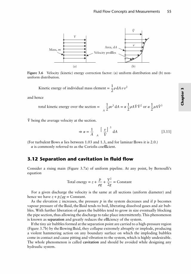
Fluid Flow Concepts and Measurements 55
V
V–
νMass, m
Area, dA
Velocity profiles
(b)(a)
Figure 3.6 Velocity (kinetic) energy correction factor: (a) uniform distribution and (b) non-uniform distribution.
Kinetic energy of individual mass element = 12𝜌dA v v2
and hence
total kinetic energy over the section = ∫A
12𝜌v3 dA = 𝛼
12𝜌AVV2 or 𝛼 1
2𝜌AV3
V being the average velocity at the section.
⇒ 𝛼 = 1A ∫A
(vV
)3
dA [3.11]
(For turbulent flows 𝛼 lies between 1.03 and 1.3, and for laminar flows it is 2.0.)𝛼 is commonly referred to as the Coriolis coefficient.
3.12 Separation and cavitation in fluid flow
Consider a rising main (Figure 3.7a) of uniform pipeline. At any point, by Bernoulli’sequation
Total energy = z +p𝜌g
+ V2
2g= Constant
For a given discharge the velocity is the same at all sections (uniform diameter) andhence we have z + p∕𝜌g = Constant.
As the elevation z increases, the pressure p in the system decreases and if p becomesvapour pressure of the fluid, the fluid tends to boil, liberating dissolved gases and air bub-bles. With further liberation of gases the bubbles tend to grow in size eventually blockingthe pipe section, thus allowing the discharge to take place intermittently. This phenomenonis known as separation and greatly reduces the efficiency of the system.
If the tiny air bubbles formed at the separation point are carried to a high-pressure region(Figure 3.7b) by the flowing fluid, they collapse extremely abruptly or implode, producinga violent hammering action on any boundary surface on which the imploding bubblescome in contact and cause pitting and vibration to the system, which is highly undesirable.The whole phenomenon is called cavitation and should be avoided while designing anyhydraulic system.
Ch
apte
r3
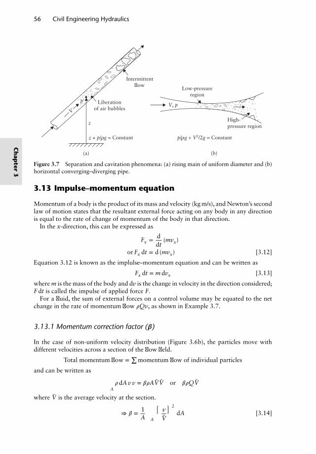
56 Civil Engineering Hydraulics
Liberationof air bubbles
Intermittentflow
Low-pressureregion
V, pV
High-pressure region
z + p/ g = Constant
z
p/ g + V2/2g = Constant
(b)(a)
p
ρ ρ
Figure 3.7 Separation and cavitation phenomena: (a) rising main of uniform diameter and (b)horizontal converging–diverging pipe.
3.13 Impulse–momentum equation
Momentum of a body is the product of its mass and velocity (kg m/s), and Newton’s secondlaw of motion states that the resultant external force acting on any body in any directionis equal to the rate of change of momentum of the body in that direction.
In the x-direction, this can be expressed as
Fx = ddt
(mvx)
or Fx dt = d (mvx) [3.12]
Equation 3.12 is known as the implulse–momentum equation and can be written as
Fx dt = m dvx [3.13]
where m is the mass of the body and dv is the change in velocity in the direction considered;F dt is called the impulse of applied force F.
For a fluid, the sum of external forces on a control volume may be equated to the netchange in the rate of momentum flow 𝜌Qv, as shown in Example 3.7.
3.13.1 Momentum correction factor (𝜷)
In the case of non-uniform velocity distribution (Figure 3.6b), the particles move withdifferent velocities across a section of the flow field.
Total momentum flow =∑
momentum flow of individual particles
and can be written as
∫A𝜌dA v v = 𝛽𝜌AVV or 𝛽𝜌QV
where V is the average velocity at the section.
⇒ 𝛽 = 1A ∫A
(vV
)2
dA [3.14]
Ch
apter
3
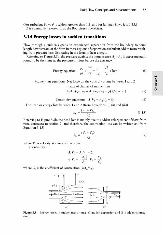
Fluid Flow Concepts and Measurements 57
(For turbulent flows 𝛽 is seldom greater than 1.1, and for laminar flows it is 1.33.)𝛽 is commonly referred to as the Boussinesq coefficient.
3.14 Energy losses in sudden transitions
Flow through a sudden expansion experiences separation from the boundary to somelength downstream of the flow. In these regions of separation, turbulent eddies form result-ing from pressure loss dissipating in the form of heat energy.
Referring to Figure 3.8a, the pressure against the annular area A2 – A1 is experimentallyfound to be the same as the pressure p1, just before the entrance.
Energy equation:p1
𝜌g+
V21
2g=
p2
𝜌g+
V22
2g+ loss (i)
Momentum equation: Net force on the control volume between 1 and 2
= rate of change of momentum
p1A1 + p1(A2 − A1) − p2A2 = 𝜌Q(V2 − V1) (ii)
Continuity equation: A1V1 = A2V2 = Q (iii)
The head or energy loss between 1 and 2 (from Equations (i), (ii) and (iii))
hL =(V1 − V2)2
2g[3.15]
Referring to Figure 3.8b, the head loss is mainly due to sudden enlargement of flow fromvena contracta to section 2, and therefore, the contraction loss can be written as (fromEquation 3.15)
hL =(Vc − V2)2
2g(iv)
where Vc is velocity at vena contracta v–c.By continuity,
AcVc = A2V2 = Q
⇒ Vc =(
A2
Ac
)V2 =
V2
Cc
where Cc is the coefficient of contraction (=Ac∕A2).
(b)(a)
2
c
v
–121
p1/ gp2/ g
ρρ
Figure 3.8 Energy losses in sudden transitions: (a) sudden expansion and (b) sudden contrac-tion.
Ch
apte
r3
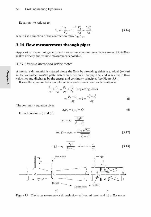
58 Civil Engineering Hydraulics
Equation (iv) reduces to
hL =(
1Cc
− 1)2 V2
2
2g=
kV22
2g[3.16]
where k is a function of the contraction ratio A2∕A1.
3.15 Flow measurement through pipes
Application of continuity, energy and momentum equations to a given system of fluid flowmakes velocity and volume measurements possible.
3.15.1 Venturi meter and orifice meter
A pressure differential is created along the flow by providing either a gradual (venturimeter) or sudden (orifice plate meter) constriction in the pipeline, and is related to flowvelocities and discharge by the energy and continuity principles (see Figure 3.9).
Bernoulli’s equation between inlet section and constriction can be written as
p1
𝜌g+
v21
2g=
p2
𝜌g+
v22
2gneglecting losses
⇒p1 − p2
𝜌g= h =
v21 − v2
2
2g(i)
The continuity equation givesa1v1 = a2v2 = Q (ii)
From Equations (i) and (ii),
v1 = a2
√2gh
a21 − a2
2
and Q = a1v1 =a1a2
√2gh√
a21 − a2
2
[3.17]
or Q = a1
√2gh
k2 − 1where k =
a1
a2[3.18]
(b)(a)
Throat
Piezometer
ConstrictionOrifice
d1
h h
d2 d2
10° 3°
Figure 3.9 Discharge measurement through pipes: (a) venturi meter and (b) orifice meter.
Ch
apter
3
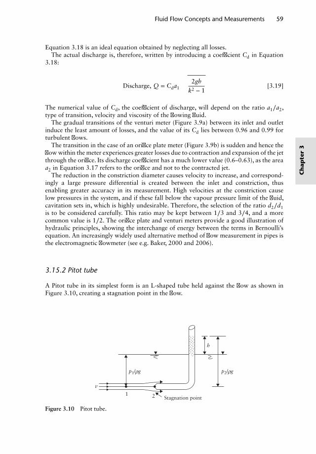
Fluid Flow Concepts and Measurements 59
Equation 3.18 is an ideal equation obtained by neglecting all losses.The actual discharge is, therefore, written by introducing a coefficient Cd in Equation
3.18:
Discharge, Q = Cda1
√2gh
k2 − 1[3.19]
The numerical value of Cd, the coefficient of discharge, will depend on the ratio a1∕a2,type of transition, velocity and viscosity of the flowing fluid.
The gradual transitions of the venturi meter (Figure 3.9a) between its inlet and outletinduce the least amount of losses, and the value of its Cd lies between 0.96 and 0.99 forturbulent flows.
The transition in the case of an orifice plate meter (Figure 3.9b) is sudden and hence theflow within the meter experiences greater losses due to contraction and expansion of the jetthrough the orifice. Its discharge coefficient has a much lower value (0.6–0.63), as the areaa2 in Equation 3.17 refers to the orifice and not to the contracted jet.
The reduction in the constriction diameter causes velocity to increase, and correspond-ingly a large pressure differential is created between the inlet and constriction, thusenabling greater accuracy in its measurement. High velocities at the constriction causelow pressures in the system, and if these fall below the vapour pressure limit of the fluid,cavitation sets in, which is highly undesirable. Therefore, the selection of the ratio d2∕d1is to be considered carefully. This ratio may be kept between 1∕3 and 3∕4, and a morecommon value is 1∕2. The orifice plate and venturi meters provide a good illustration ofhydraulic principles, showing the interchange of energy between the terms in Bernoulli’sequation. An increasingly widely used alternative method of flow measurement in pipes isthe electromagnetic flowmeter (see e.g. Baker, 2000 and 2006).
3.15.2 Pitot tube
A Pitot tube in its simplest form is an L-shaped tube held against the flow as shown inFigure 3.10, creating a stagnation point in the flow.
2 Stagnation point1
p1/ g p2/ g
v
h
ρ ρ
Figure 3.10 Pitot tube.
Ch
apte
r3
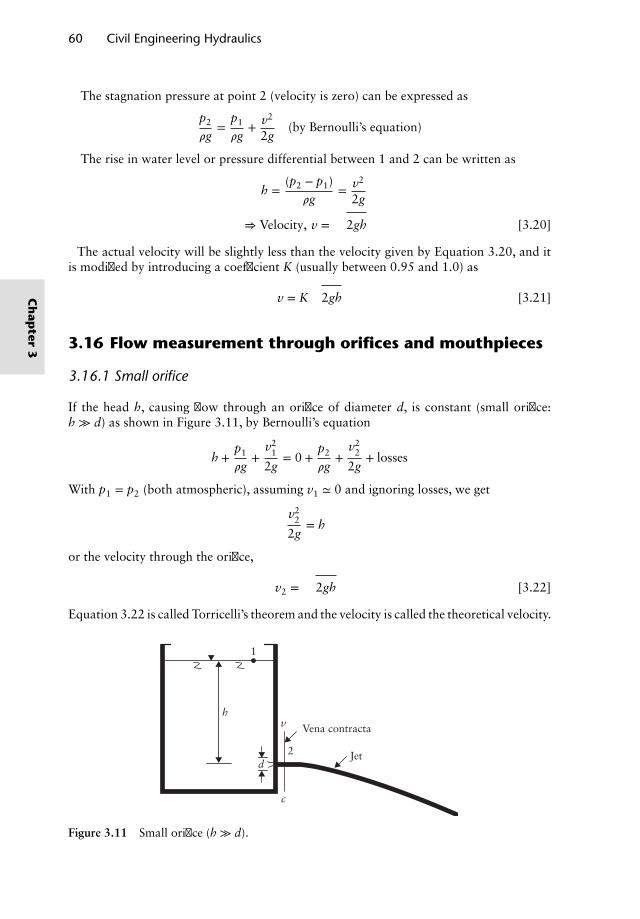
60 Civil Engineering Hydraulics
The stagnation pressure at point 2 (velocity is zero) can be expressed as
p2
𝜌g=
p1
𝜌g+ v2
2g(by Bernoulli’s equation)
The rise in water level or pressure differential between 1 and 2 can be written as
h =(p2 − p1)
𝜌g= v2
2g
⇒ Velocity, v =√
2gh [3.20]
The actual velocity will be slightly less than the velocity given by Equation 3.20, and itis modified by introducing a coefficient K (usually between 0.95 and 1.0) as
v = K√
2gh [3.21]
3.16 Flow measurement through orifices and mouthpieces
3.16.1 Small orifice
If the head h, causing flow through an orifice of diameter d, is constant (small orifice:h ≫ d) as shown in Figure 3.11, by Bernoulli’s equation
h +p1
𝜌g+
v21
2g= 0 +
p2
𝜌g+
v22
2g+ losses
With p1 = p2 (both atmospheric), assuming v1 ≃ 0 and ignoring losses, we get
v22
2g= h
or the velocity through the orifice,
v2 =√
2gh [3.22]
Equation 3.22 is called Torricelli’s theorem and the velocity is called the theoretical velocity.
Vena contracta
Jet
v
1
c
2
h
d
Figure 3.11 Small orifice (h ≫ d).
Ch
apter
3
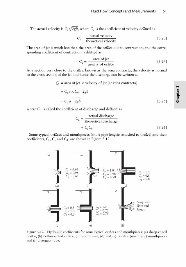
Fluid Flow Concepts and Measurements 61
The actual velocity is Cv
√2gh, where Cv is the coefficient of velocity defined as
Cv =actual velocity
theoretical velocity[3.23]
The area of jet is much less than the area of the orifice due to contraction, and the corre-sponding coefficient of contraction is defined as
Cc =area of jet
area a of orifice[3.24]
At a section very close to the orifice, known as the vena contracta, the velocity is normalto the cross section of the jet and hence the discharge can be written as
Q = area of jet × velocity of jet (at vena contracta)
= Cc a × Cv
√2gh
= Cd a√
2gh [3.25]
where Cd is called the coefficient of discharge and defined as
Cd =actual discharge
theoretical discharge
= CcCv [3.26]
Some typical orifices and mouthpieces (short pipe lengths attached to orifice) and theircoefficients, Cc, Cv and Cd, are shown in Figure 3.12.
Cc = 0.62Cv = 0.98Cd = 0.61
Cc = 1.0Cv = 0.98Cd = 0.98
Cc = 1.0Cv = 0.8Cd = 0.8
Cc = 0.5Cv = 1.0Cd = 0.5
Cc = 1.0
Vary withflare andlengthCv = 0.75
Cd = 0.75
(a) (b)
r
(c)
(f)(e)(d)
Figure 3.12 Hydraulic coefficients for some typical orifices and mouthpieces: (a) sharp-edgedorifice, (b) bell-mouthed orifice, (c) mouthpiece, (d) and (e) Borda’s (re-entrant) mouthpiecesand (f) divergent tube.
Ch
apte
r3
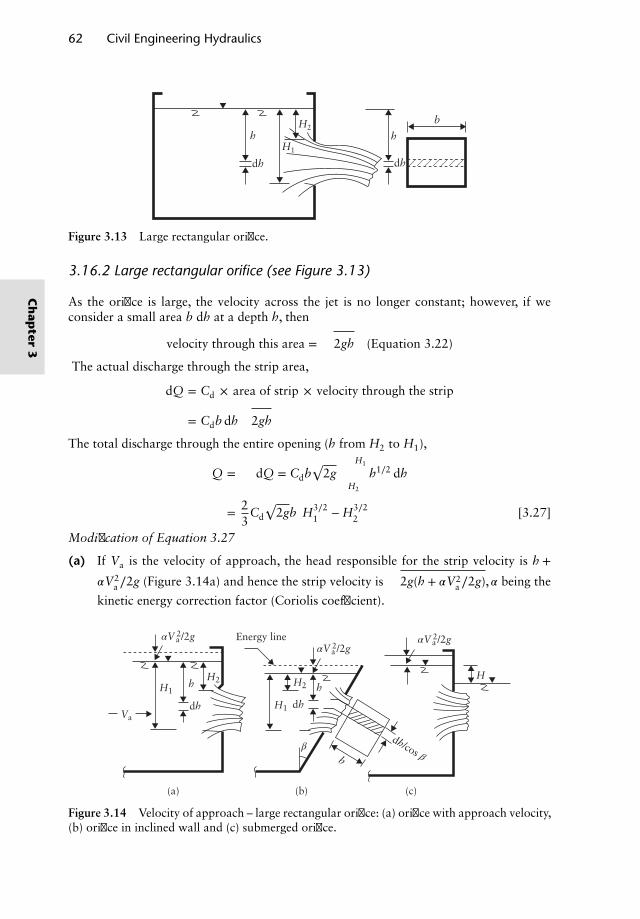
62 Civil Engineering Hydraulics
h h
b
dh dh
H2
H1
Figure 3.13 Large rectangular orifice.
3.16.2 Large rectangular orifice (see Figure 3.13)
As the orifice is large, the velocity across the jet is no longer constant; however, if weconsider a small area b dh at a depth h, then
velocity through this area =√
2gh (Equation 3.22)
The actual discharge through the strip area,
dQ = Cd × area of strip × velocity through the strip
= Cdb dh√
2gh
The total discharge through the entire opening (h from H2 to H1),
Q = ∫ dQ = Cdb√
2g ∫H1
H2
h1∕2 dh
= 23
Cd
√2gb
(H3∕2
1 − H3∕22
)[3.27]
Modification of Equation 3.27
(a) If Va is the velocity of approach, the head responsible for the strip velocity is h +𝛼V2
a∕2g (Figure 3.14a) and hence the strip velocity is√
2g(h + 𝛼V2a∕2g),𝛼 being the
kinetic energy correction factor (Coriolis coefficient).
αVa2/2g
αVa2/2g
αVa2/2g
β
Va
H1
H1
H2 H2H
dh dh
h h
b
dh/cos β
Energy line
(c)(b)(a)
Figure 3.14 Velocity of approach – large rectangular orifice: (a) orifice with approach velocity,(b) orifice in inclined wall and (c) submerged orifice.
Ch
apter
3
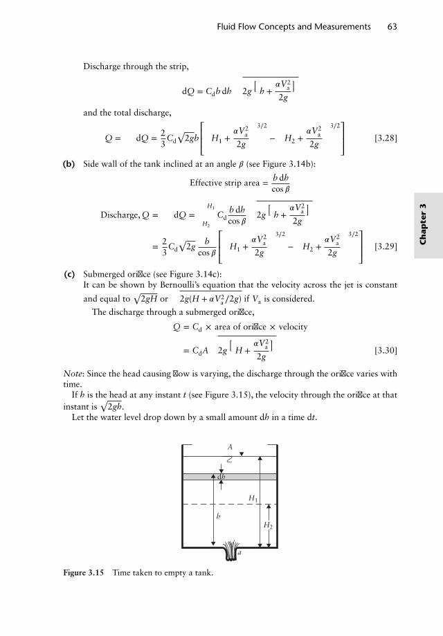
Fluid Flow Concepts and Measurements 63
Discharge through the strip,
dQ = Cdb dh
√2g
(h +
𝛼V2a
2g
)
and the total discharge,
Q = ∫ dQ = 23
Cd
√2gb
⎡⎢⎢⎣(
H1 +𝛼V2
a
2g
)3∕2
−
(H2 +
𝛼V2a
2g
)3∕2⎤⎥⎥⎦ [3.28]
(b) Side wall of the tank inclined at an angle 𝛽 (see Figure 3.14b):
Effective strip area = b dhcos 𝛽
Discharge, Q = ∫ dQ = ∫H1
H2
Cdb dhcos 𝛽
√2g
(h +
𝛼V2a
2g
)
= 23
Cd
√2g
bcos 𝛽
⎡⎢⎢⎣(
H1 +𝛼V2
a
2g
)3∕2
−
(H2 +
𝛼V2a
2g
)3∕2⎤⎥⎥⎦ [3.29]
(c) Submerged orifice (see Figure 3.14c):It can be shown by Bernoulli’s equation that the velocity across the jet is constant
and equal to√
2gH or√
2g(H + 𝛼V2a∕2g) if Va is considered.
The discharge through a submerged orifice,
Q = Cd × area of orifice × velocity
= CdA
√2g
(H +
𝛼V2a
2g
)[3.30]
Note: Since the head causing flow is varying, the discharge through the orifice varies withtime.
If h is the head at any instant t (see Figure 3.15), the velocity through the orifice at thatinstant is
√2gh.
Let the water level drop down by a small amount dh in a time dt.
A
h
a
H2
H1
dh
Figure 3.15 Time taken to empty a tank.
Ch
apte
r3
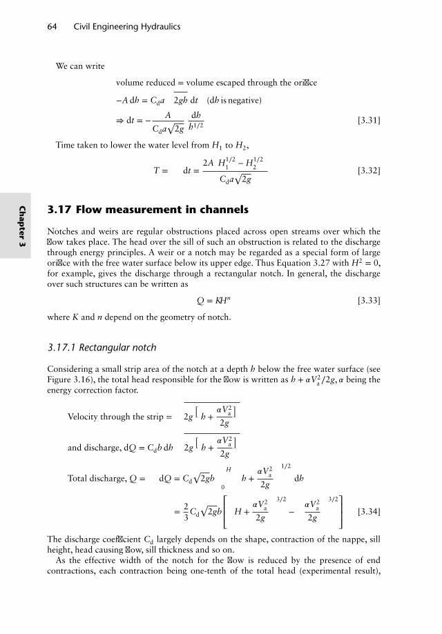
64 Civil Engineering Hydraulics
We can write
volume reduced = volume escaped through the orifice
−A dh = Cda√
2gh dt (dh is negative)
⇒ dt = − A
Cda√
2g
dhh1∕2
[3.31]
Time taken to lower the water level from H1 to H2,
T = ∫ dt =2A
(H1∕2
1 − H1∕22
)Cda
√2g
[3.32]
3.17 Flow measurement in channels
Notches and weirs are regular obstructions placed across open streams over which theflow takes place. The head over the sill of such an obstruction is related to the dischargethrough energy principles. A weir or a notch may be regarded as a special form of largeorifice with the free water surface below its upper edge. Thus Equation 3.27 with H2 = 0,for example, gives the discharge through a rectangular notch. In general, the dischargeover such structures can be written as
Q = KHn [3.33]
where K and n depend on the geometry of notch.
3.17.1 Rectangular notch
Considering a small strip area of the notch at a depth h below the free water surface (seeFigure 3.16), the total head responsible for the flow is written as h + 𝛼V2
a∕2g, 𝛼 being theenergy correction factor.
Velocity through the strip =
√2g
(h +
𝛼V2a
2g
)
and discharge, dQ = Cdb dh
√2g
(h +
𝛼V2a
2g
)
Total discharge, Q = ∫ dQ = Cd
√2gb∫
H
0
(h +
𝛼V2a
2g
)1∕2
dh
= 23
Cd
√2gb
⎡⎢⎢⎣(
H +𝛼V2
a
2g
)3∕2
−
(𝛼V2
a
2g
)3∕2⎤⎥⎥⎦ [3.34]
The discharge coefficient Cd largely depends on the shape, contraction of the nappe, sillheight, head causing flow, sill thickness and so on.
As the effective width of the notch for the flow is reduced by the presence of endcontractions, each contraction being one-tenth of the total head (experimental result),
Ch
apter
3
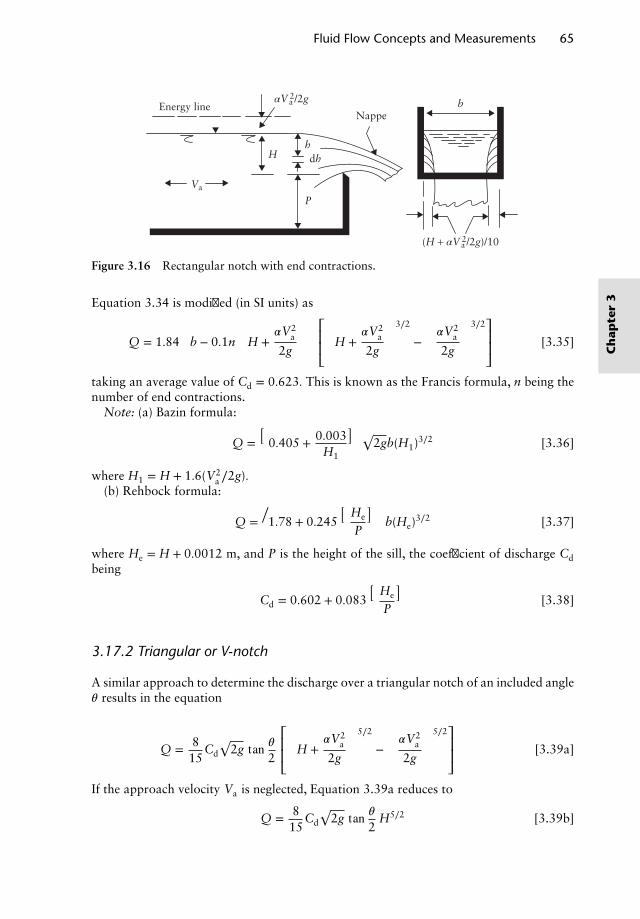
Fluid Flow Concepts and Measurements 65
αVa2/2g
Va
H
P
b
dh
(H + αVa2/2g)/10
h
Energy lineNappe
Figure 3.16 Rectangular notch with end contractions.
Equation 3.34 is modified (in SI units) as
Q = 1.84
[b − 0.1n
(H +
𝛼V2a
2g
)]⎡⎢⎢⎣(
H +𝛼V2
a
2g
)3∕2
−
(𝛼V2
a
2g
)3∕2⎤⎥⎥⎦ [3.35]
taking an average value of Cd = 0.623. This is known as the Francis formula, n being thenumber of end contractions.
Note: (a) Bazin formula:
Q =(
0.405 + 0.003H1
) √2gb(H1)3∕2 [3.36]
where H1 = H + 1.6(V2a∕2g).
(b) Rehbock formula:
Q =[1.78 + 0.245
(He
P
)]b(He)
3∕2 [3.37]
where He = H + 0.0012 m, and P is the height of the sill, the coefficient of discharge Cdbeing
Cd = 0.602 + 0.083(
He
P
)[3.38]
3.17.2 Triangular or V-notch
A similar approach to determine the discharge over a triangular notch of an included angle𝜃 results in the equation
Q = 815
Cd
√2g tan 𝜃
2
⎡⎢⎢⎣(
H +𝛼V2
a
2g
)5∕2
−
(𝛼V2
a
2g
)5∕2⎤⎥⎥⎦ [3.39a]
If the approach velocity Va is neglected, Equation 3.39a reduces to
Q = 815
Cd
√2g tan 𝜃
2H5∕2 [3.39b]
Ch
apte
r3
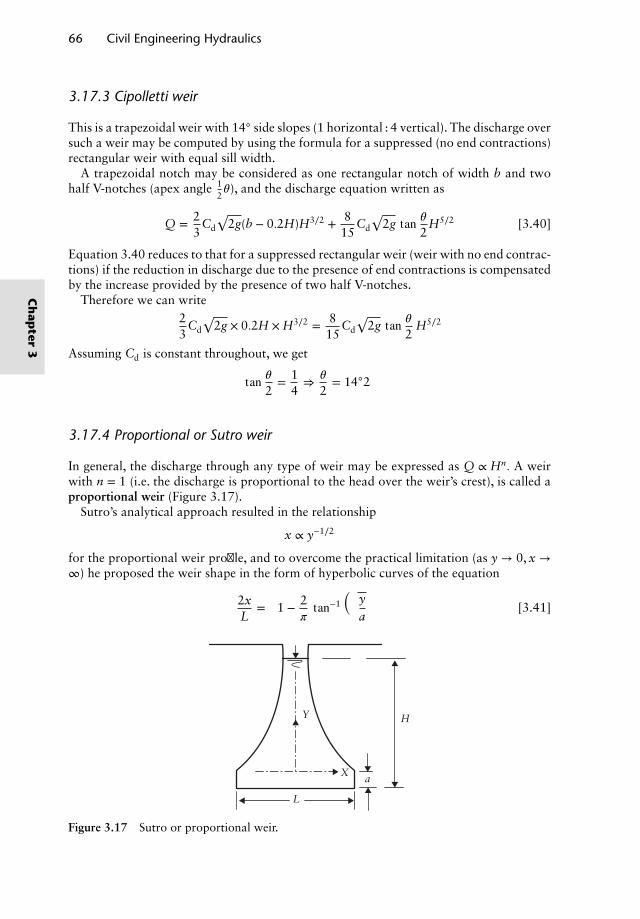
66 Civil Engineering Hydraulics
3.17.3 Cipolletti weir
This is a trapezoidal weir with 14◦ side slopes (1 horizontal : 4 vertical). The discharge oversuch a weir may be computed by using the formula for a suppressed (no end contractions)rectangular weir with equal sill width.
A trapezoidal notch may be considered as one rectangular notch of width b and twohalf V-notches (apex angle 1
2𝜃), and the discharge equation written as
Q = 23
Cd
√2g(b − 0.2H)H3∕2 + 8
15Cd
√2g tan 𝜃
2H5∕2 [3.40]
Equation 3.40 reduces to that for a suppressed rectangular weir (weir with no end contrac-tions) if the reduction in discharge due to the presence of end contractions is compensatedby the increase provided by the presence of two half V-notches.
Therefore we can write23
Cd
√2g × 0.2H × H3∕2 = 8
15Cd
√2g tan 𝜃
2H5∕2
Assuming Cd is constant throughout, we get
tan 𝜃2= 1
4⇒
𝜃
2= 14◦2′
3.17.4 Proportional or Sutro weir
In general, the discharge through any type of weir may be expressed as Q ∝ Hn. A weirwith n = 1 (i.e. the discharge is proportional to the head over the weir’s crest), is called aproportional weir (Figure 3.17).
Sutro’s analytical approach resulted in the relationship
x ∝ y−1∕2
for the proportional weir profile, and to overcome the practical limitation (as y → 0, x →∞) he proposed the weir shape in the form of hyperbolic curves of the equation
2xL
=
[1 − 2
𝜋tan−1
√ya
][3.41]
Y H
X a
L
Figure 3.17 Sutro or proportional weir.
Ch
apter
3
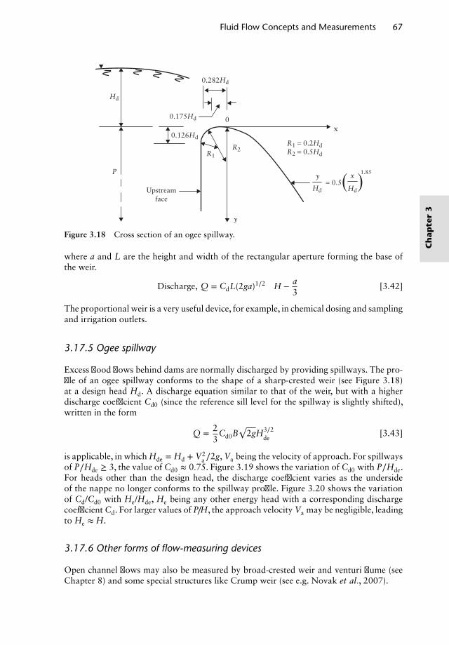
Fluid Flow Concepts and Measurements 67
Hd
P
y
R2R1
0.126HdR1 = 0.2HdR2 = 0.5Hd
1.85
0.175Hd 0x
0.282Hd
Upstreamface
y
Hd= 0.5
x
Hd
Figure 3.18 Cross section of an ogee spillway.
where a and L are the height and width of the rectangular aperture forming the base ofthe weir.
Discharge, Q = CdL(2ga)1∕2(
H − a3
)[3.42]
The proportional weir is a very useful device, for example, in chemical dosing and samplingand irrigation outlets.
3.17.5 Ogee spillway
Excess flood flows behind dams are normally discharged by providing spillways. The pro-file of an ogee spillway conforms to the shape of a sharp-crested weir (see Figure 3.18)at a design head Hd. A discharge equation similar to that of the weir, but with a higherdischarge coefficient Cd0 (since the reference sill level for the spillway is slightly shifted),written in the form
Q = 23
Cd0B√
2gH3∕2de
[3.43]
is applicable, in which Hde = Hd + V2a∕2g, Va being the velocity of approach. For spillways
of P∕Hde ≥ 3, the value of Cd0 ≈ 0.75. Figure 3.19 shows the variation of Cd0 with P∕Hde.For heads other than the design head, the discharge coefficient varies as the undersideof the nappe no longer conforms to the spillway profile. Figure 3.20 shows the variationof Cd/Cd0 with He/Hde, He being any other energy head with a corresponding dischargecoefficient Cd. For larger values of P∕H, the approach velocity Va may be negligible, leadingto He ≈ H.
3.17.6 Other forms of flow-measuring devices
Open channel flows may also be measured by broad-crested weir and venturi flume (seeChapter 8) and some special structures like Crump weir (see e.g. Novak et al., 2007).
Ch
apte
r3
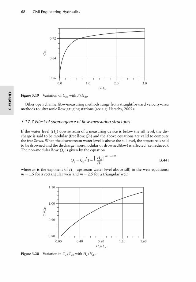
68 Civil Engineering Hydraulics
0.0
0.56
0.64
0.72
1.0
P/Hde
3.02.0
Cd0
Figure 3.19 Variation of Cd0 with P∕Hde.
Other open channel flow-measuring methods range from straightforward velocity–areamethods to ultrasonic flow gauging stations (see e.g. Herschy, 2009).
3.17.7 Effect of submergence of flow-measuring structures
If the water level (H2) downstream of a measuring device is below the sill level, the dis-charge is said to be modular (free flow, Qf) and the above equations are valid to computethe free flows. When the downstream water level is above the sill level, the structure is saidto be drowned and the discharge (non-modular or drowned flow) is affected (i.e. reduced).The non-modular flow Qs is given by the equation
Qs = Qf
[1 −
(H2
H1
)m]0.385
[3.44]
where m is the exponent of H1 (upstream water level above sill) in the weir equations:m = 1.5 for a rectangular weir and m = 2.5 for a triangular weir.
0.00
0.80
0.90
1.00
1.10
0.40
He/Hde
1.601.200.80
Cd/
Cd0
Figure 3.20 Variation in Cd∕Cd0 with He∕Hde.
Ch
apter
3
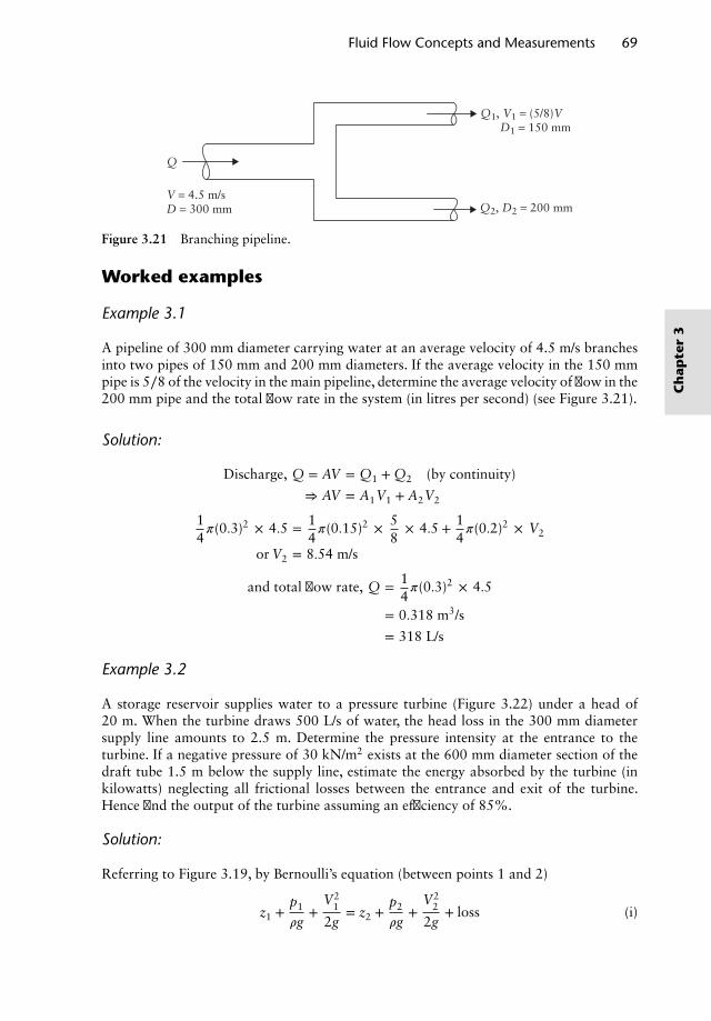
Fluid Flow Concepts and Measurements 69
Q
V = 4.5 m/sD = 300 mm
Q1, V1 = (5/8)VD1 = 150 mm
Q2, D2 = 200 mm
Figure 3.21 Branching pipeline.
Worked examples
Example 3.1
A pipeline of 300 mm diameter carrying water at an average velocity of 4.5 m/s branchesinto two pipes of 150 mm and 200 mm diameters. If the average velocity in the 150 mmpipe is 5∕8 of the velocity in the main pipeline, determine the average velocity of flow in the200 mm pipe and the total flow rate in the system (in litres per second) (see Figure 3.21).
Solution:
Discharge, Q = AV = Q1 + Q2 (by continuity)
⇒ AV = A1V1 + A2V2
14𝜋(0.3)2 × 4.5 = 1
4𝜋(0.15)2 × 5
8× 4.5 + 1
4𝜋(0.2)2 × V2
or V2 = 8.54 m/s
and total flow rate, Q = 14𝜋(0.3)2 × 4.5
= 0.318 m3/s
= 318 L/s
Example 3.2
A storage reservoir supplies water to a pressure turbine (Figure 3.22) under a head of20 m. When the turbine draws 500 L/s of water, the head loss in the 300 mm diametersupply line amounts to 2.5 m. Determine the pressure intensity at the entrance to theturbine. If a negative pressure of 30 kN/m2 exists at the 600 mm diameter section of thedraft tube 1.5 m below the supply line, estimate the energy absorbed by the turbine (inkilowatts) neglecting all frictional losses between the entrance and exit of the turbine.Hence find the output of the turbine assuming an efficiency of 85%.
Solution:
Referring to Figure 3.19, by Bernoulli’s equation (between points 1 and 2)
z1 +p1
𝜌g+
V21
2g= z2 +
p2
𝜌g+
V22
2g+ loss (i)
Ch
apte
r3
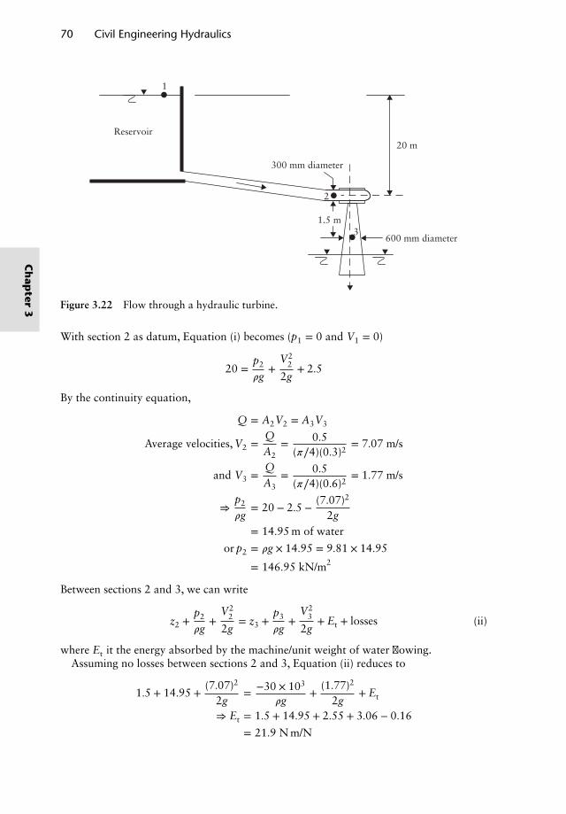
70 Civil Engineering Hydraulics
Reservoir
300 mm diameter
600 mm diameter
2
31.5 m
20 m
1
Figure 3.22 Flow through a hydraulic turbine.
With section 2 as datum, Equation (i) becomes (p1 = 0 and V1 = 0)
20 =p2
𝜌g+
V22
2g+ 2.5
By the continuity equation,
Q = A2V2 = A3V3
Average velocities,V2 =QA2
= 0.5(𝜋∕4)(0.3)2
= 7.07 m/s
and V3 =QA3
= 0.5(𝜋∕4)(0.6)2
= 1.77 m/s
⇒p2
𝜌g= 20 − 2.5 − (7.07)2
2g= 14.95 m of water
or p2 = 𝜌g × 14.95 = 9.81 × 14.95
= 146.95 kN/m2
Between sections 2 and 3, we can write
z2 +p2
𝜌g+
V22
2g= z3 +
p3
𝜌g+
V23
2g+ Et + losses (ii)
where Et it the energy absorbed by the machine/unit weight of water flowing.Assuming no losses between sections 2 and 3, Equation (ii) reduces to
1.5 + 14.95 + (7.07)2
2g= −30 × 103
𝜌g+ (1.77)2
2g+ Et
⇒ Et = 1.5 + 14.95 + 2.55 + 3.06 − 0.16
= 21.9 N m/N
Ch
apter
3
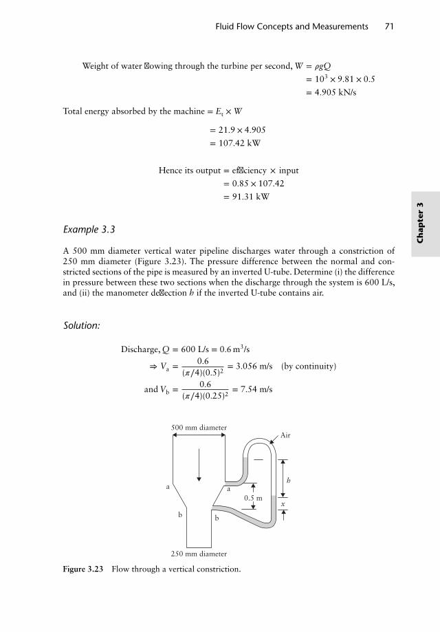
Fluid Flow Concepts and Measurements 71
Weight of water flowing through the turbine per second, W = 𝜌gQ
= 103 × 9.81 × 0.5
= 4.905 kN/s
Total energy absorbed by the machine = Et × W
= 21.9 × 4.905
= 107.42 kW
Hence its output = efficiency × input
= 0.85 × 107.42
= 91.31 kW
Example 3.3
A 500 mm diameter vertical water pipeline discharges water through a constriction of250 mm diameter (Figure 3.23). The pressure difference between the normal and con-stricted sections of the pipe is measured by an inverted U-tube. Determine (i) the differencein pressure between these two sections when the discharge through the system is 600 L/s,and (ii) the manometer deflection h if the inverted U-tube contains air.
Solution:
Discharge, Q = 600 L/s = 0.6 m3/s
⇒ Va = 0.6(𝜋∕4)(0.5)2
= 3.056 m/s (by continuity)
and Vb = 0.6(𝜋∕4)(0.25)2
= 7.54 m/s
500 mm diameter
250 mm diameter
Air
h
x0.5 m
aa
bb
Figure 3.23 Flow through a vertical constriction.
Ch
apte
r3
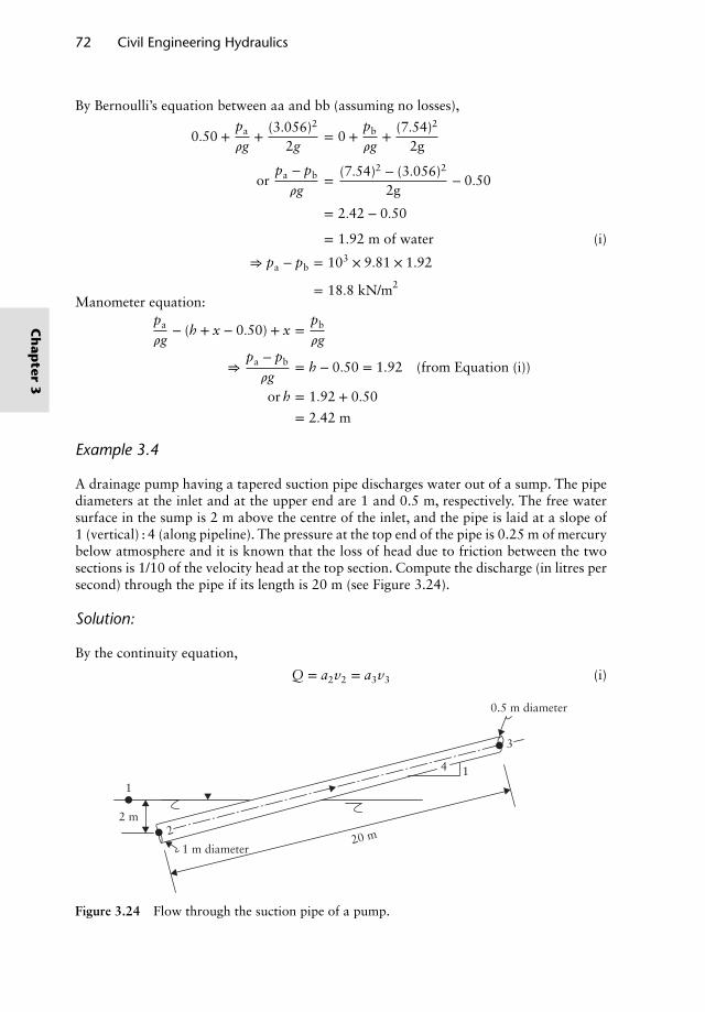
72 Civil Engineering Hydraulics
By Bernoulli’s equation between aa and bb (assuming no losses),
0.50 +pa
𝜌g+
(3.056)2
2g= 0 +
pb
𝜌g+
(7.54)2
2g
orpa − pb
𝜌g=
(7.54)2 − (3.056)2
2g− 0.50
= 2.42 − 0.50
= 1.92 m of water (i)
⇒ pa − pb = 103 × 9.81 × 1.92
= 18.8 kN/m2
Manometer equation:pa
𝜌g− (h + x − 0.50) + x =
pb
𝜌g
⇒pa − pb
𝜌g= h − 0.50 = 1.92 (from Equation (i))
or h = 1.92 + 0.50
= 2.42 m
Example 3.4
A drainage pump having a tapered suction pipe discharges water out of a sump. The pipediameters at the inlet and at the upper end are 1 and 0.5 m, respectively. The free watersurface in the sump is 2 m above the centre of the inlet, and the pipe is laid at a slope of1 (vertical) : 4 (along pipeline). The pressure at the top end of the pipe is 0.25 m of mercurybelow atmosphere and it is known that the loss of head due to friction between the twosections is 1/10 of the velocity head at the top section. Compute the discharge (in litres persecond) through the pipe if its length is 20 m (see Figure 3.24).
Solution:
By the continuity equation,
Q = a2v2 = a3v3 (i)
3
14
0.5 m diameter
2 m
1
20 m1 m diameter
2
Figure 3.24 Flow through the suction pipe of a pump.
Ch
apter
3
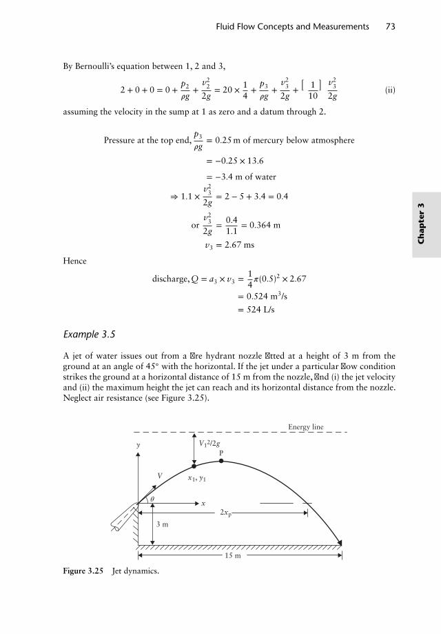
Fluid Flow Concepts and Measurements 73
By Bernoulli’s equation between 1, 2 and 3,
2 + 0 + 0 = 0 +p2
𝜌g+
v22
2g= 20 × 1
4+
p3
𝜌g+
v23
2g+(
110
) v23
2g(ii)
assuming the velocity in the sump at 1 as zero and a datum through 2.
Pressure at the top end,p3
𝜌g= 0.25 m of mercury below atmosphere
= −0.25 × 13.6
= −3.4 m of water
⇒ 1.1 ×v2
3
2g= 2 − 5 + 3.4 = 0.4
orv2
3
2g= 0.4
1.1= 0.364 m
v3 = 2.67 ms
Hence
discharge,Q = a3 × v3 = 14𝜋(0.5)2 × 2.67
= 0.524 m3/s
= 524 L/s
Example 3.5
A jet of water issues out from a fire hydrant nozzle fitted at a height of 3 m from theground at an angle of 45◦ with the horizontal. If the jet under a particular flow conditionstrikes the ground at a horizontal distance of 15 m from the nozzle, find (i) the jet velocityand (ii) the maximum height the jet can reach and its horizontal distance from the nozzle.Neglect air resistance (see Figure 3.25).
P
Energy line
2xp
15 m
3 m
V
x
x1, y1
θ
V12/2gy
Figure 3.25 Jet dynamics.
Ch
apte
r3
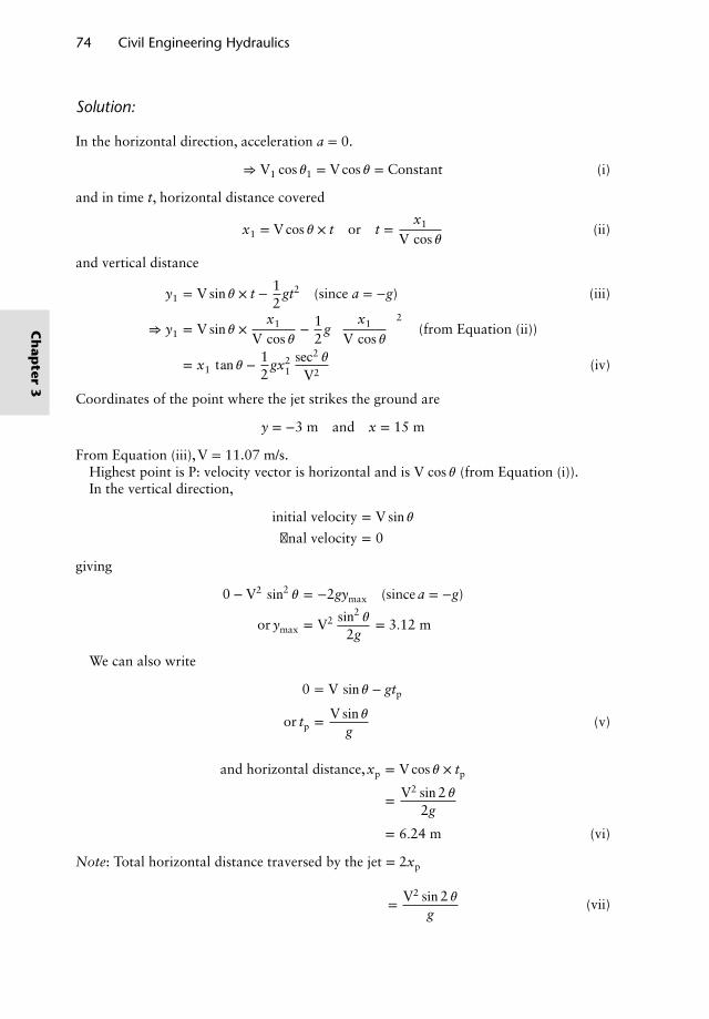
74 Civil Engineering Hydraulics
Solution:
In the horizontal direction, acceleration a = 0.
⇒ V1 cos 𝜃1 = V cos 𝜃 = Constant (i)
and in time t, horizontal distance covered
x1 = V cos 𝜃 × t or t =x1
V cos 𝜃(ii)
and vertical distance
y1 = V sin 𝜃 × t − 12
gt2 (since a = −g) (iii)
⇒ y1 = V sin 𝜃 ×x1
V cos 𝜃− 1
2g( x1
V cos 𝜃
)2(from Equation (ii))
= x1 tan 𝜃 − 12
gx21sec2 𝜃
V2(iv)
Coordinates of the point where the jet strikes the ground are
y = −3 m and x = 15 m
From Equation (iii),V = 11.07 m/s.Highest point is P: velocity vector is horizontal and is V cos 𝜃 (from Equation (i)).In the vertical direction,
initial velocity = V sin 𝜃final velocity = 0
giving
0 − V2 sin2𝜃 = −2gymax (since a = −g)
or ymax = V2 sin2𝜃
2g= 3.12 m
We can also write
0 = V sin 𝜃 − gtp
or tp = V sin 𝜃g
(v)
and horizontal distance,xp = V cos 𝜃 × tp
= V2 sin 2 𝜃2g
= 6.24 m (vi)
Note: Total horizontal distance traversed by the jet = 2xp
= V2 sin 2 𝜃g
(vii)
Ch
apter
3
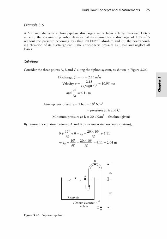
Fluid Flow Concepts and Measurements 75
Example 3.6
A 500 mm diameter siphon pipeline discharges water from a large reservoir. Deter-mine (i) the maximum possible elevation of its summit for a discharge of 2.15 m3/swithout the pressure becoming less than 20 kN/m2 absolute and (ii) the correspond-ing elevation of its discharge end. Take atmospheric pressure as 1 bar and neglect alllosses.
Solution:
Consider the three points A, B and C along the siphon system, as shown in Figure 3.26.
Discharge,Q = av = 2.15 m3/s
Velocity,v = 2.15(𝜋∕4)(0.5)2
= 10.95 m/s
and v2
2g= 6.11 m
Atmospheric pressure = 1 bar = 105 N/m2
= pressures at A and C
Minimum pressure at B = 20 kN/m2 absolute (given)
By Bernoulli’s equation between A and B (reservoir water surface as datum),
0 + 105
𝜌g+ 0 = zB + 20 × 103
𝜌g+ 6.11
⇒ zB = 105
𝜌g− 20 × 103
𝜌g− 6.11 = 2.04 m
zC
zB
B
A
Reservoir
500 mm diametersiphon C
Figure 3.26 Siphon pipeline.
Ch
apte
r3
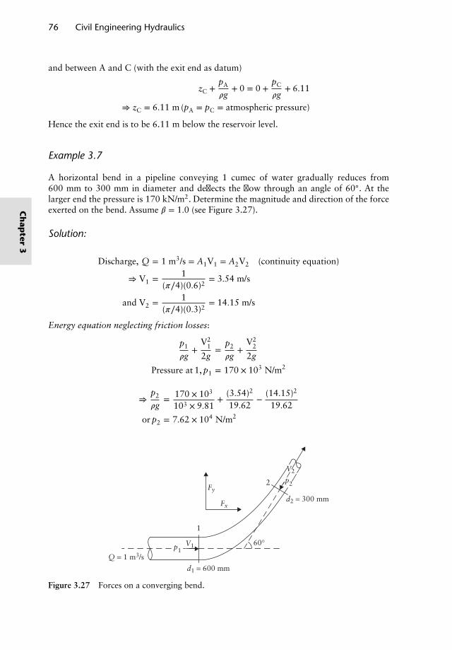
76 Civil Engineering Hydraulics
and between A and C (with the exit end as datum)
zC +pA
𝜌g+ 0 = 0 +
pC
𝜌g+ 6.11
⇒ zC = 6.11 m (pA = pC = atmospheric pressure)
Hence the exit end is to be 6.11 m below the reservoir level.
Example 3.7
A horizontal bend in a pipeline conveying 1 cumec of water gradually reduces from600 mm to 300 mm in diameter and deflects the flow through an angle of 60◦. At thelarger end the pressure is 170 kN/m2. Determine the magnitude and direction of the forceexerted on the bend. Assume 𝛽 = 1.0 (see Figure 3.27).
Solution:
Discharge, Q = 1 m3/s = A1V1 = A2V2 (continuity equation)
⇒ V1 = 1(𝜋∕4)(0.6)2
= 3.54 m/s
and V2 = 1(𝜋∕4)(0.3)2
= 14.15 m/s
Energy equation neglecting friction losses:
p1
𝜌g+
V21
2g=
p2
𝜌g+
V22
2g
Pressure at 1, p1 = 170 × 103 N/m2
⇒p2
𝜌g= 170 × 103
103 × 9.81+ (3.54)2
19.62− (14.15)2
19.62
or p2 = 7.62 × 10⁴ N/m2
d1 = 600 mm
d2 = 300 mm
Q = 1 m3/s
Fy
Fx
p1V1
p2
V2
1
2
60°
Figure 3.27 Forces on a converging bend.
Ch
apter
3
Fluid Flow Concepts and Measurements 77
Momentum equation: Gravity forces are zero along the horizontal plane and the onlyforces acting on the fluid mass are pressure and momentum forces.
Let Fx and Fy be the two components of the total force F exerted by the bent boundarysurface on the fluid mass; these are considered positive if Fx is left to right and Fy upwards.
In the x-direction,
p1A1 + Fx − p2A2 cos 𝜃 = 𝜌Q (V2 cos 𝜃 − V1)
and in the y-direction,
0 + Fy − p2A2 sin 𝜃 = 𝜌Q (V2 sin 𝜃 − 0)
⇒ Fx = 103 × 1(14.15 cos60◦ − 3.54) + 7.62 × 104 × 14𝜋(0.3)2 cos60◦
−17 × 104 × 14𝜋(0.6)2
= −4.2 × 10⁴ N (negative sign indicates Fx is right to left)
and Fy = 103 × 1(14.15 sin60◦) + 7.62 × 104 × 14𝜋(0.3)2 sin 60◦
= 1.7 × 10⁴ N (upwards)
According to Newton’s third law of motion, the forces Rx and Ry exerted by the fluidon the bend will be equal and opposite to Fx and Fy.
⇒ Rx = −Fx = 4.2 × 10⁴ N (left to right)
and Ry = −Fy = −1.7 × 10⁴ N (downwards)
Resultant force on the bend,
R =√
R2x + R2
y
= 4.53 × 10⁴ N or 45.3 kN
Acting at an angle, 𝜃 = tan−1(Ry
Rx
)= 22◦ to the x-direction
Example 3.8
Derive an expression for the normal force on a plate inclined at 𝜃◦ to the jet.A 150 mm × 150 mm square metal plate, 10 mm thick, is hinged about a horizontal
edge. If a 10 mm diameter horizontal jet of water impinging 50 mm below the hinge keepsthe plate inclined at 30◦ to the vertical, find the velocity of the jet. Take the specific weightof the metal as 75 kN/m3.
Solution:
Referring to Figure 3.28a, force in the normal direction to the plate,
F = (mass × change in velocity normal to the plate) of jet
F = 𝜌aV [V cos(90◦ − 𝜃) − 0]
= 𝜌aV2 sin 𝜃N
Ch
apte
r3
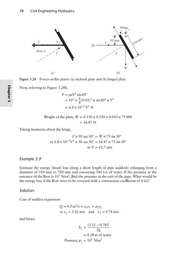
78 Civil Engineering Hydraulics
Hinge
30°
(b)(a)
Jet
50 mm
Area, aFF
VθV
W
150 mm
Figure 3.28 Forces on flat plates: (a) inclined plate and (b) hinged plate.
Now, referring to Figure 3.28b,
F = 𝜌aV2 sin 60◦
= 103 × 𝜋
4(0.01)2 × sin 60◦ × V2
= 6.8 × 10⁻² V2 N
Weight of the plate, W = 0.150 × 0.150 × 0.010 × 75 000
= 16.87 N
Taking moments about the hinge,
F × 50 sec30◦ = W × 75 sin30◦
or 6.8 × 10⁻²V2 × 50 sec30◦ = 16.87 × 75 sin30◦
⇒ V = 12.7 m/s
Example 3.9
Estimate the energy (head) loss along a short length of pipe suddenly enlarging from adiameter of 350 mm to 700 mm and conveying 300 L/s of water. If the pressure at theentrance of the flow is 105 N/m2, find the pressure at the exit of the pipe. What would bethe energy loss if the flow were to be reversed with a contraction coefficient of 0.62?
Solution:
Case of sudden expansion:
Q = 0.3 m3/s = a1v1 = a2v2
⇒ v1 = 3.12 m/s and v2 = 0.78 m/s
and hence
hL = (3.12 − 0.78)2
2g= 0.28 m of water
Pressure, p1 = 105 N/m2
Ch
apter
3
Fluid Flow Concepts and Measurements 79
By energy equation,p1
𝜌g+
v21
2g=
p2
𝜌g+
v22
2g+
(v1 − v2)2
2g
10.2 + 0.5 =p2
𝜌g+ 0.03 + 0.28
⇒p2
𝜌g= 10.39 m or p2 = 1.02 × 10⁵ N/m2
Case of sudden contraction:
hL =[(1∕Cc) − 1]2v2
2g(where v is the velocity in the smaller pipe)
=[(1∕0.62) − 1]2(3.12)2
2g= 0.186 m of water
Example 3.10
A venturi meter is introduced in a 300 mm diameter horizontal pipeline carrying waterunder a pressure of 150 kN/m2. The throat diameter of the meter is 100 mm and thepressure at the throat is 400 mm of mercury below atmosphere. If 3% of the differentialpressure is lost between inlet and throat, determine the flow rate in the pipeline.
Solution:
Bernoulli’s equation between inlet and throat:
p1
𝜌g+
v21
2g=
p2
𝜌g+
v22
2g+ 0.03
(p1
𝜌g−
p2
𝜌g
)
⇒0.97(p1 − p2)
𝜌g=
(v22 − v2
1)
2g
p1 = 150 × 103 N/m2 = 15.29 m of water
p2 = −400 mm of mercury = −0.4 × 13.6 m of water
= −5.44 m of water
⇒p1 − p2
𝜌g= 15.29 − (−5.44)
= 20.73 mand hence
v22 − v2
1
2g= 0.97 × 20.73
= 20.11 m (i)From the continuity equation, a1v1 = a2v2
⇒ v1 =(
a2
a1
)v2 =
(d2
d1
)2
v2
=(
1030
)2
v2
=(
19
)v2 (ii)
Ch
apte
r3
80 Civil Engineering Hydraulics
From Equations (i) and (ii),
v22 (1 − 1∕81)
2g= 20.11
or
v2 =
√2g × 20.111 − 1∕81
= 19.89 m/s
Flow rate, Q = a2v2 = 14𝜋(0.1)2 × 19.98
= 0.157 m3/s or 157 L/s
Example 3.11
A 50 mm × 25 mm venturi meter with a coefficient of discharge of 0.98 is to be replaced byan orifice meter having a coefficient of discharge of 0.6. If both meters are to give the samedifferential mercury manometer reading for a discharge of 10 L/s, determine the diameterof the orifice.
Solution:
Discharge through venturi meter = discharge through orifice meter
k = a1∕a2 = (50∕25)2 = 4 for the venturi meter and ko for the orifice meter = (50∕do)2,where do is the diameter of orifice.
Q = 0.01 = 0.98 × 14𝜋(0.05)2
√2gh
42 − 1
= 0.6 × 14𝜋(0.05)2
√2gh
k2o − 1
or
√k2
o − 1 =0.6
√15
0.98
⇒ ko =(
50do
)2
= 2.57 or do = 50√2.57
= 31.2 mm
Example 3.12
A Pitot tube was used to measure the quantity of water flowing in a pipe of 300 mmdiameter. The stagnation pressure at the centre line of the pipe is 250 mm of water morethan the static pressure. If the mean velocity is 0.78 times the centre line velocity and thecoefficient of the Pitot tube is 0.98, find the rate of flow in litres per second.
Ch
apter
3
Fluid Flow Concepts and Measurements 81
Solution:
The centre line velocity in the pipe, v = K√
2gh
= 0.98√
2 × 9.81 × 0.25
= 2.17 m/s
Mean velocity of flow = 0.78 × 2.17
= 1.693 m/s
Hence
discharge, Q = av
= 14𝜋(0.3)2 × 1.693
= 0.12 m3/s or 120 L/s
Example 3.13
A large rectangular orifice 0.40 m wide and 0.60 m deep, placed with the upper edge in ahorizontal position 0.90 m vertically below the water surface in a vertical side wall of alarge tank, is discharging to atmosphere. Calculate the rate of flow through the orifice ifits discharge coefficient is 0.65.
Solution:
The discharge rate when b = 0.4 m, H1 = 0.90 + 0.60 = 1.5 m, H2 = 0.90 m and Cd =0.65 from Equation 3.27,
Q = 23× 0.65 ×
√2g × 0.40 ×
[(1.5)3∕2 − (0.9)3∕2]
= 0.755 m3/s
Example 3.14
A vertical circular tank 1.25 m diameter is fitted with a sharp-edged circular orifice50 mm in diameter in its base. When the flow of water into the tank was shut off, thetime taken to lower the head from 2 to 0.75 m was 253 s. Determine the rate of flow (inlitres per second) through the orifice under a steady head of 1.5 m.
Solution:
T = 253 s, H1 = 2 m, H2 = 0.75 m, a = 14𝜋(0.05)2 = 1.96 × 10⁻³ m2 and A = 1
4𝜋(1.25)2 =
1.228 m2.From Equation 3.32, Cd = 0.61.
Ch
apte
r3
82 Civil Engineering Hydraulics
Hence steady discharge under a head of 1.5 m
= Cda√
2gH
= 0.61 × 1.96 × 10−3 ×√
2g × (1.5)1∕2
= 0.0065 m3/s or 6.5 L/s
Example 3.15
Determine the discharge over a sharp-crested weir 4.5 m long with no lateral contractions,the measured head over the crest being 0.45 m. The width of the approach channel is4.5 m and the sill height of the weir is 1 m.
Solution:
Equation 3.35 is rewritten as
Q = 1.84b⎡⎢⎢⎣(
H +V2
a
2g
)3∕2
−
(V2
a
2g
)3∕2⎤⎥⎥⎦ (i)
for a weir with no lateral contractions (suppressed weir) and 𝛼 = 1.Equation (i) reduces to
Q = 1.84b(H)3∕2 (ii)
neglecting velocity of approach as a first approximation.From Equation (ii),
Q = 1.84 × 4.5 × (0.45)3∕2
= 2.5 m3/s
Now velocity of approach, Va = 2.54.5 (1 + 0.45)
= 0.383 m/s
andV2
a
2g= 7.48 × 10⁻³ m
⇒ Q = 1.84 × 4.5[(0.45 + 0.00748)3∕2 − (0.00748)3∕2]
= 2.556 m3/s
Example 3.16
The discharge over a triangular notch can be written as
Q =(
815
)Cd
√2g tan 𝜃
2H5∕2
If an error of 1% in measuring H is introduced, determine the corresponding error inthe computed discharge.
Ch
apter
3
Fluid Flow Concepts and Measurements 83
A right-angled triangular notch is used for gauging the flow of a laboratory flume. Ifthe coefficient of discharge of the notch is 0.593 and an error of 2 mm is suspected inobserving the head, find the percentage error in computing an estimated discharge of 20L/s.
Solution:
We can write
Q = KH5∕2
⇒ dQ =(
52
)KH3∕2 dH
and
dQQ
=(5∕2) KH3∕2 dH
KH5∕2
=(
52
)dHH
(i)
If dH/H is 1%, the error in the discharge dQ/Q = 2.5% (from Equation (i)).
Q = 0.02 = 815
× 0.593 ×√
2g × 1 × H5∕2
or
H5∕2 = 1.4275 × 10⁻²
or
H = 0.183 m or 183 mm
and
dQQ
= 2.5 × dHH
= 2.5 × 2183
= 2.73%
Example 3.17
If the velocity distribution of a turbulent flow in an open channel is given by a power law
vvmax
=(
yy0
)1∕7
where v is the velocity at a distance y from the bed and vmax is the maximum velocity inthe channel with a flow depth of y0, determine the average velocity and the energy (𝛼) andmomentum (𝛽) correction factors. Assume the flow to be two-dimensional.
Ch
apte
r3
84 Civil Engineering Hydraulics
Solution:
If the mean velocity of flow is V, the discharge per unit width of the channel is
y0V = q = ∫y0
0v dy
which gives q = (7∕8)vmaxy0.
Therefore
V =qy0
=(
78
)vmax
The kinetic energy correction factor 𝛼, given by Equation 3.11, can be written as
𝛼 = 1A ∫
A
( vV
)3dA = 1
y0V3 ∫y0
0
[vmax
(yy0
)1∕7]3
dy
Replacing vmax [= (8∕7)V] and integrating, we obtain 𝛼 = 1.045. The momentum correc-tion factor 𝛽 given by Equation 3.14 can be written as
𝛽 = 1A ∫
A
( vV
)2dA = 1
y0V2 ∫y0
0
[vmax
(yy0
)1∕7]2
dy
Again replacing vmax and integrating, we obtain 𝛽 = 1.016.Note: The energy and momentum correction factors 𝛼 and 𝛽 for open channels may be
computed by the equations
𝛼 = 1 + 3𝜀2 − 2𝜀3 and 𝛽 = 1 + 𝜀2 where 𝜀 =vmax
V− 1
If the velocity distributions are not described by any equation and if the measured data areavailable, 𝛼 and 𝛽 values may be computed by graphical methods; plots of ∫ v dy, ∫ v3 dyand ∫ v2 dy will help to give V, 𝛼 and 𝛽, respectively.
Example 3.18
An ogee spillway of large height is to be designed to evacuate a flood discharge of 200 m3/sunder a head of 2 m. The spillway is spanned by piers to support a bridge deck above. Theclear span between piers is limited to 6 m. Determine the number of spans required in orderto pass the flood discharge with the head not exceeding 2 m. Assume the pier contractioncoefficient kp = 0.01 and the abutment contraction coefficient ka = 0.10.
Solution:
The flow between the piers and abutments is contracted, thus reducing the spillway widthfor the flow to Be. Each pier has two end contractions and one abutment, and hence theeffective width is given by
Be = B − 2(nkp + ka)He
n being the number of piers.
Ch
apter
3
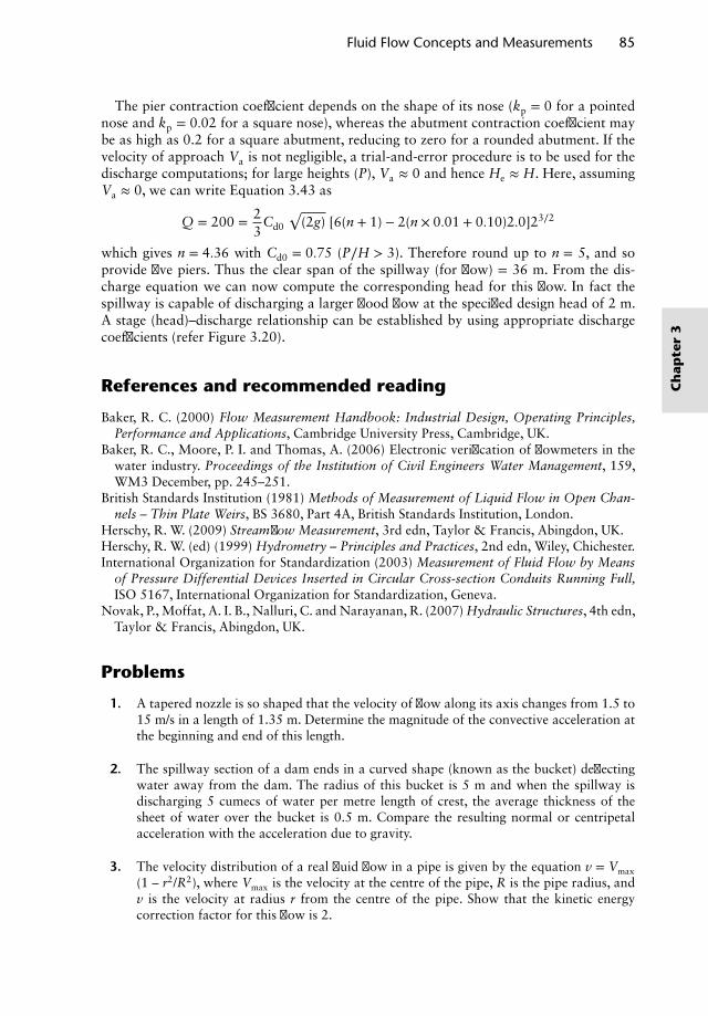
Fluid Flow Concepts and Measurements 85
The pier contraction coefficient depends on the shape of its nose (kp = 0 for a pointednose and kp = 0.02 for a square nose), whereas the abutment contraction coefficient maybe as high as 0.2 for a square abutment, reducing to zero for a rounded abutment. If thevelocity of approach Va is not negligible, a trial-and-error procedure is to be used for thedischarge computations; for large heights (P), Va ≈ 0 and hence He ≈ H. Here, assumingVa ≈ 0, we can write Equation 3.43 as
Q = 200 = 23
Cd0
√(2g) [6(n + 1) − 2(n × 0.01 + 0.10)2.0]23∕2
which gives n = 4.36 with Cd0 = 0.75 (P∕H > 3). Therefore round up to n = 5, and soprovide five piers. Thus the clear span of the spillway (for flow) = 36 m. From the dis-charge equation we can now compute the corresponding head for this flow. In fact thespillway is capable of discharging a larger flood flow at the specified design head of 2 m.A stage (head)–discharge relationship can be established by using appropriate dischargecoefficients (refer Figure 3.20).
References and recommended reading
Baker, R. C. (2000) Flow Measurement Handbook: Industrial Design, Operating Principles,Performance and Applications, Cambridge University Press, Cambridge, UK.
Baker, R. C., Moore, P. I. and Thomas, A. (2006) Electronic verification of flowmeters in thewater industry. Proceedings of the Institution of Civil Engineers Water Management, 159,WM3 December, pp. 245–251.
British Standards Institution (1981) Methods of Measurement of Liquid Flow in Open Chan-nels – Thin Plate Weirs, BS 3680, Part 4A, British Standards Institution, London.
Herschy, R. W. (2009) Streamflow Measurement, 3rd edn, Taylor & Francis, Abingdon, UK.Herschy, R. W. (ed) (1999) Hydrometry – Principles and Practices, 2nd edn, Wiley, Chichester.International Organization for Standardization (2003) Measurement of Fluid Flow by Means
of Pressure Differential Devices Inserted in Circular Cross-section Conduits Running Full,ISO 5167, International Organization for Standardization, Geneva.
Novak, P., Moffat, A. I. B., Nalluri, C. and Narayanan, R. (2007) Hydraulic Structures, 4th edn,Taylor & Francis, Abingdon, UK.
Problems
1. A tapered nozzle is so shaped that the velocity of flow along its axis changes from 1.5 to15 m/s in a length of 1.35 m. Determine the magnitude of the convective acceleration atthe beginning and end of this length.
2. The spillway section of a dam ends in a curved shape (known as the bucket) deflectingwater away from the dam. The radius of this bucket is 5 m and when the spillway isdischarging 5 cumecs of water per metre length of crest, the average thickness of thesheet of water over the bucket is 0.5 m. Compare the resulting normal or centripetalacceleration with the acceleration due to gravity.
3. The velocity distribution of a real fluid flow in a pipe is given by the equation v = Vmax(1 – r2/R2), where Vmax is the velocity at the centre of the pipe, R is the pipe radius, andv is the velocity at radius r from the centre of the pipe. Show that the kinetic energycorrection factor for this flow is 2.
Ch
apte
r3
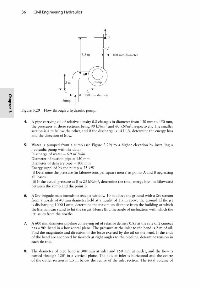
86 Civil Engineering Hydraulics
150 mm diameter
Sump
Pump3 m
4.5 m
B
100 mm diameter
A
Figure 3.29 Flow through a hydraulic pump.
4. A pipe carrying oil of relative density 0.8 changes in diameter from 150 mm to 450 mm,the pressures at these sections being 90 kN/m2 and 60 kN/m2, respectively. The smallersection is 4 m below the other, and if the discharge is 145 L/s, determine the energy lossand the direction of flow.
5. Water is pumped from a sump (see Figure 3.29) to a higher elevation by installing ahydraulic pump with the data:Discharge of water = 6.9 m3/minDiameter of suction pipe = 150 mmDiameter of delivery pipe = 100 mmEnergy supplied by the pump = 25 kW(i) Determine the pressure (in kilonewtons per square metre) at points A and B neglectingall losses.(ii) If the actual pressure at B is 25 kN/m2, determine the total energy loss (in kilowatts)between the sump and the point B.
6. A fire-brigade man intends to reach a window 10 m above the ground with a fire streamfrom a nozzle of 40 mm diameter held at a height of 1.5 m above the ground. If the jetis discharging 1000 L/min, determine the maximum distance from the building at whichthe fireman can stand to hit the target. Hence find the angle of inclination with which thejet issues from the nozzle.
7. A 600 mm diameter pipeline conveying oil of relative density 0.85 at the rate of 2 cumecshas a 90◦ bend in a horizontal plane. The pressure at the inlet to the bend is 2 m of oil.Find the magnitude and direction of the force exerted by the oil on the bend. If the endsof the bend are anchored by tie-rods at right angles to the pipeline, determine tension ineach tie-rod.
8. The diameter of pipe bend is 300 mm at inlet and 150 mm at outlet, and the flow isturned through 120◦ in a vertical plane. The axis at inlet is horizontal and the centreof the outlet section is 1.5 m below the centre of the inlet section. The total volume of
Ch
apter
3
Fluid Flow Concepts and Measurements 87
fluid contained in the bend is 8.5 × 10⁻² m3. Neglecting friction, calculate the magnitudeand direction of the force exerted on the bend by water flowing through it at a rate of0.225 m3/s when the inlet pressure is 140 kN/m2.
9. A sluice gate is used to control the flow of water in a horizontal rectangular channel,6 m wide. The gate is lowered so that the stream flowing under it has a depth of 800 mmand a velocity of 12 m/s. The depth upstream of the sluice gate is 7 m. Determine theforce exerted by the water on the sluice gate, assuming uniform velocity distribution inthe channel and neglecting frictional losses.
10. A 50 mm diameter jet of water strikes a curved vane at rest with a velocity of 30 m/sand is deflected through 45◦ from its original direction. Neglecting friction, compute theresultant force on the vane in magnitude and direction.
11. A horizontal rectangular outlet downstream of a dam, 2.5 m high and 1.5 m wide, dis-charges 70 m3/s of water on to a concave concrete floor of 12 m radius and 6 m length,deflecting the water away from the outlet to dissipate energy. Calculate the resultantthrust the fluid exerts on the floor.
12. A venturi meter is to be fitted to a pipe of 250 mm diameter where the pressure head is 6m of water and the maximum flow is 9 m3/min. Find the smallest diameter of the throatto ensure that the pressure head does not become negative.
13. (a) Determine the diameter of throat of a venturi meter to be introduced in a horizon-tal section of a 100 mm diameter main so that deflection of a differential mercurymanometer connected between the inlet and throat is 600 mm when the discharge is20 L/s of water. The discharge coefficient of the meter is 0.95.
(b) What difference will it make to the manometer reading if the meter is introduced ina vertical length of the pipeline, with water flowing upwards, and the distance frominlet to throat of the meter is 200 mm?
14. A Pitot tube placed in front of a submarine moving horizontally in sea water 16 m belowthe water surface is connected to the two limbs of a U-tube mercury manometer. Findthe speed of the submarine for a manometer deflection of 200 mm. Relative densities ofmercury and sea water are 13.6 and 1.026, respectively.
15. In an experiment to determine the hydraulic coefficients of a 25 mm diameter sharp-edged orifice, it was found that the jet issuing horizontally under a head of 1 m travelleda horizontal distance of 1.5 m from the vena contracta in the course of a vertical drop of612 mm from the same point. Furthermore, the impact force of the jet on a flat plate heldnormal to it at the vena contracta was measured as 5.5 N. Determine the three coefficientsof the orifice, assuming an impact coefficient of unity.
16. A swimming pool with vertical sides is 25 m long and 10 m wide. Water at the deep endis 2.5 m and shallow end 1 m. If there are two outlets each 500 mm diameter, one ateach of the deep and shallow ends, find the time taken to empty the pool. Assume thedischarge coefficients for both the outlets as 0.8.
17. A convergent–divergent nozzle is fitted to the vertical side of a tank containing water toa height of 2 m above the centre line of the nozzle. Find the throat and exit diameters
Ch
apte
r3
88 Civil Engineering Hydraulics
of the nozzle if it discharges 7 L/s of water into the atmosphere, assuming that (i) thepressure head in the throat is 2.5 m of water absolute, (ii) atmospheric pressure is 10 mof water, (iii) there is no hydraulic loss in the convergent part of the nozzle, and (iv) thehead loss in the divergent part is 1/5 of exit velocity head.
18. When water flows through a right-angled V-notch, show that the discharge is given byQ = KH5∕2, in which k is a dimensional constant and H is the height of water surfaceabove the bottom of the notch. (i) What are the dimensions of K if H is in metres andQ in metres cubed per second? (ii) Determine the head causing flow when the dischargethrough this notch is 1.42 L/s. Take Cd = 0.62. (iii) Find the accuracy with which the headin (ii) must be measured if the error in the estimation of discharge is not to exceed 1.5%.
19. (a) What is meant by a ‘suppressed’ weir? Explain the precautions that you would takein using such a weir as a discharge-measuring structure.
(b) A suppressed weir with two ventilating pipes is installed in a laboratory flume withthe following data:
Width of flume = 1000 mmHeight of weir, P = 300 mmDiameter of ventilating pipes = 30 mmPressure difference between the two sides of the nappe = 1 N/m2
Head over sill, h = 150 mmDensity of air = 1.25 kg/m3
Coefficient of discharge, Cd = 0.611 + 0.075(h/P)Assuming a smooth entrance to the ventilating pipes and neglecting the velocity ofapproach, find the air demand in terms of percentage of water discharge.
20. State the advantages of a triangular weir over a rectangular one, for measuring discharges.The following observations of head and the corresponding discharge were made in a
laboratory to calibrate a 90◦ V-notch.
Head (mm) 50 75 100 125 150Discharge (L/s) 0.81 2.24 4.76 8.03 12.66
Determine K and n in the discharge equation, Q = KHn (H in metres and Q in metrescubed per second) and hence find the value of the coefficient of discharge.
21. A reservoir has an area of 8.5 ha and is provided with a weir 4.5 m long (Cd = 0.6).Find how long it will take for the water level above the sill to fall from 0.60 to 0.30 m.
Ch
apter
3
Chapter 4Flow of IncompressibleFluids in Pipelines
4.1 Resistance in circular pipelines flowing full
A fluid moving through a pipeline is subjected to energy losses from various sources. Acontinuous resistance is exerted by the pipe walls due to the formation of a boundarylayer in which the velocity decreases from the centre of the pipe to zero at the boundary.In steady flow in a uniform pipeline the boundary shear stress 𝜏0 is constant along the pipe,since the boundary layer is of constant thickness, and this resistance results in a uniformrate of total energy or head degradation along the pipeline. The total head loss along aspecified length of pipeline is commonly referred to as the ‘head loss due to friction’ anddenoted by hf. The rate of energy loss or energy gradient Sf = hf∕L.
The hydraulic grade line shows the elevation of the pressure head along the pipe. In auniform pipe the velocity head 𝛼V2∕2g is constant and the energy grade line is parallel tothe hydraulic grade line (Figure 4.1). Applying Bernoulli’s equation to sections 1 and 2,
z1 +p1
𝜌g+𝛼V2
1
2g= z2 +
p2
𝜌g+𝛼V2
2
2g+ hf
and since V1 = V2,
z1 +p1
𝜌g= z2 +
p2
𝜌g+ hf [4.1]
In steady uniform flow the motivating and drag forces are exactly balanced. Equatingbetween sections 1 and 2,
(p1 − p2)A + 𝜌gAL sin 𝜃 = 𝜏0PL [4.2]
where A is the area of cross section, P the wetted perimeter and 𝜏0 the boundary shearstress.
Nalluri & Featherstone’s Civil Engineering Hydraulics: Essential Theory with Worked Examples,Sixth Edition. Martin Marriott.© 2016 John Wiley & Sons, Ltd. Published 2016 by John Wiley & Sons, Ltd.Companion Website: www.wiley.com/go/Marriott
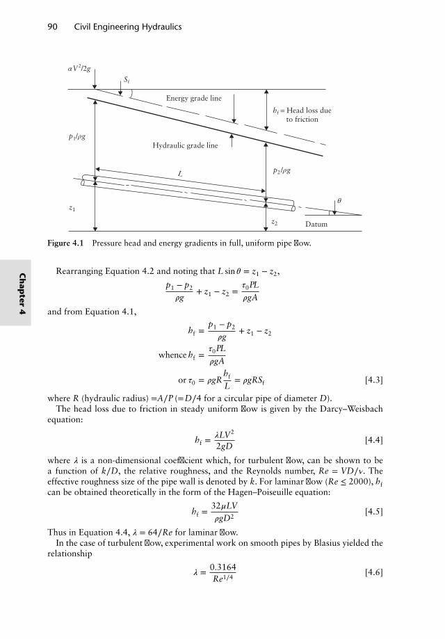
90 Civil Engineering Hydraulics
z1
z2
p1/ρg
p2/ρg
θ
αV2/2g
Sf
hf = Head loss due to friction
L
Energy grade line
Hydraulic grade line
Datum
Figure 4.1 Pressure head and energy gradients in full, uniform pipe flow.
Rearranging Equation 4.2 and noting that L sin 𝜃 = z1 − z2,
p1 − p2
𝜌g+ z1 − z2 =
𝜏0PL
𝜌gA
and from Equation 4.1,
hf =p1 − p2
𝜌g+ z1 − z2
whence hf =𝜏0PL
𝜌gA
or 𝜏0 = 𝜌gRhf
L= 𝜌gRSf [4.3]
where R (hydraulic radius) =A∕P (=D∕4 for a circular pipe of diameter D).The head loss due to friction in steady uniform flow is given by the Darcy–Weisbach
equation:
hf =𝜆LV2
2gD[4.4]
where 𝜆 is a non-dimensional coefficient which, for turbulent flow, can be shown to bea function of k∕D, the relative roughness, and the Reynolds number, Re = VD∕𝜈. Theeffective roughness size of the pipe wall is denoted by k. For laminar flow (Re ≤ 2000), hfcan be obtained theoretically in the form of the Hagen–Poiseuille equation:
hf =32𝜇LV𝜌gD2
[4.5]
Thus in Equation 4.4, 𝜆 = 64∕Re for laminar flow.In the case of turbulent flow, experimental work on smooth pipes by Blasius yielded the
relationship
𝜆 = 0.3164Re1∕4
[4.6]
Ch
apter
4
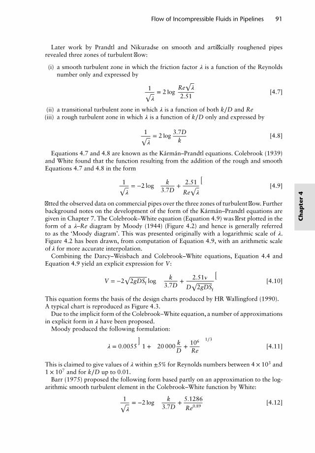
Flow of Incompressible Fluids in Pipelines 91
Later work by Prandtl and Nikuradse on smooth and artificially roughened pipesrevealed three zones of turbulent flow:
(i) a smooth turbulent zone in which the friction factor 𝜆 is a function of the Reynoldsnumber only and expressed by
1√𝜆= 2 log
Re√𝜆
2.51[4.7]
(ii) a transitional turbulent zone in which 𝜆 is a function of both k∕D and Re(iii) a rough turbulent zone in which 𝜆 is a function of k∕D only and expressed by
1√𝜆= 2 log 3.7D
k[4.8]
Equations 4.7 and 4.8 are known as the Karman–Prandtl equations. Colebrook (1939)and White found that the function resulting from the addition of the rough and smoothEquations 4.7 and 4.8 in the form
1√𝜆= −2 log
(k
3.7D+ 2.51
Re√𝜆
)[4.9]
fitted the observed data on commercial pipes over the three zones of turbulent flow. Furtherbackground notes on the development of the form of the Karman–Prandtl equations aregiven in Chapter 7. The Colebrook–White equation (Equation 4.9) was first plotted in theform of a 𝜆–Re diagram by Moody (1944) (Figure 4.2) and hence is generally referredto as the ‘Moody diagram’. This was presented originally with a logarithmic scale of 𝜆.Figure 4.2 has been drawn, from computation of Equation 4.9, with an arithmetic scaleof 𝜆 for more accurate interpolation.
Combining the Darcy–Weisbach and Colebrook–White equations, Equation 4.4 andEquation 4.9 yield an explicit expression for V:
V = −2√
2gDSf log
(k
3.7D+ 2.51𝜈
D√
2gDSf
)[4.10]
This equation forms the basis of the design charts produced by HR Wallingford (1990).A typical chart is reproduced as Figure 4.3.
Due to the implicit form of the Colebrook–White equation, a number of approximationsin explicit form in 𝜆 have been proposed.
Moody produced the following formulation:
𝜆 = 0.0055
[1 +
(20 000 k
D+ 106
Re
)1∕3]
[4.11]
This is claimed to give values of 𝜆 within ±5% for Reynolds numbers between 4 × 10³ and1 × 107 and for k∕D up to 0.01.
Barr (1975) proposed the following form based partly on an approximation to the log-arithmic smooth turbulent element in the Colebrook–White function by White:
1√𝜆= −2 log
(k
3.7D+ 5.1286
Re0.89
)[4.12]
Ch
apte
r4
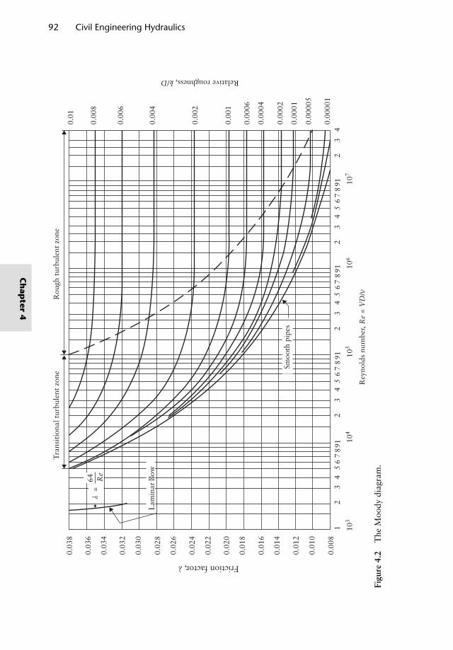
92 Civil Engineering Hydraulics
0.01
0.00
8
0.00
6
0.00
4
0.00
2
0.00
1
0.00
06
0.00
04
0.00
02
0.00
01
0.00
005
0.00
001
Relative roughness, k/D
Rey
nold
s nu
mbe
r, R
e =
VD
/
Friction factor, λλ
Rou
gh t
urbu
lent
zon
eT
rans
itio
nal t
urbu
lent
zon
e
0.03
8
64 Re
=0.
036
0.03
4
0.03
2
0.03
0
0.02
8
0.02
6
0.02
4
0.02
2
0.02
0
0.01
8
0.01
6
0.01
4
0.01
2
0.01
0
0.00
82
21
54
43
56
1919
87
87
63
24
591
87
63
24
591
87
63
2
107
106
105
104
103
Smoo
th p
ipes
Lam
inar
flow
43
Figu
re4.
2T
heM
oody
diag
ram
.
Ch
apter
4
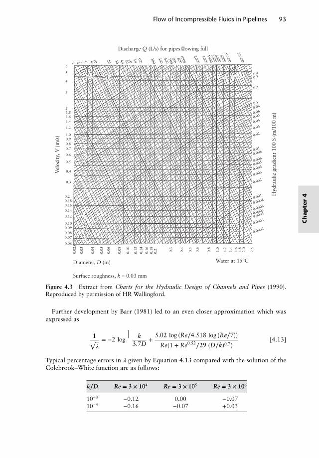
Flow of Incompressible Fluids in Pipelines 93
Discharge Q (L/s) for pipes flowing full
0.4
20 000
10000
8 000
6 000
5 000
4 000
3 000
2 000
1000
800
600500
400
300
200
100
8060504030
201086543
0.3
0.2
0.1
0.08
0.06
0.05
0.04
0.03
0.02
0.01
0.008
0.006
0.005
0.004
0.003
0.002
0.001
0.0008
0.0006
0.0005
0.0004
0.0003
0.0002
Hyd
raul
ic g
radi
ent
100
S (m
/100
m)
Vel
ocit
y, V
(m
/s)
Diameter, D (m)
Surface roughness, k = 0.03 mm
Water at 15°C
6
80 60 50 40 30 20 8 6 5 4 3 2 1 0.8 0.6 0.5
21
0.80.6
0.50.4
0.30.2
0.10.08
0.06
105
4
3
21.81.61.4
1.2
1.00.90.80.7
0.6
0.5
0.4
0.3
0.20.180.16
0.14
0.12
0.100.090.080.07
0.06
0.02
5
0.03
0.04
0.05
0.06
0.08
0.10
0.12
0.14
0.16
0.18
0.2 0.3
0.4
0.5
0.6
0.8
1.0
1.2
1.4
1.6
1.8
2.0
2.5
Figure 4.3 Extract from Charts for the Hydraulic Design of Channels and Pipes (1990).Reproduced by permission of HR Wallingford.
Further development by Barr (1981) led to an even closer approximation which wasexpressed as
1√𝜆= −2 log
[k
3.7D+
5.02 log (Re∕4.518 log (Re∕7))
Re(1 + Re0.52∕29 (D∕k)0.7)
][4.13]
Typical percentage errors in 𝜆 given by Equation 4.13 compared with the solution of theColebrook–White function are as follows:
k∕D Re = 3 × 10⁴ Re = 3 × 10⁵ Re = 3 × 10⁶
10−3 −0.12 0.00 −0.0710−4 −0.16 −0.07 +0.03
Ch
apte
r4
94 Civil Engineering Hydraulics
The values given by Equation 4.13 should be sufficiently accurate for most purposes, butsubstitution of these values once into the right-hand side of the Colebrook–White functionproduces 𝜆 values with a maximum discrepancy of +0.04%.
4.2 Resistance to flow in non-circular sections
In order to use the same form of resistance equations such as the Darcy (Equation 4.4)and Colebrook–White (Equation 4.9) equations, it is convenient to treat the non-circularsection as an equivalent hypothetical circular section yielding the same hydraulic gradientat the same discharge.
The ‘transformation’ is achieved by expressing the diameter D in terms of the hydraulicradius R = A∕P, and since for circular pipes R = D∕4, Equations 4.4 and 4.9 become
hf =𝜆LV2
8gR[4.14]
and 1√𝜆= −2 log
(k
14.8R+ 2.51𝜈
4VR√𝜆
)[4.15]
Because in the actual non-circular section the boundary shear stress is not constant aroundthe wetted perimeter whereas it is in the equivalent circular section, the ‘transformation’is not exact but experiments have shown that the error is small.
It is important to note that the equivalent circular pipe does not have the same areaas the actual conduit; their hydraulic radii are equal. Tables by HR Wallingford and Barr(2006) cover a number of non-circular cross sections, and the hydraulic performance ofovoid pipes as used in sewerage is discussed by Marriott (1996).
4.3 Local losses
In addition to the spatially continuous head loss due to friction, local head losses occur atchanges of cross section, at valves and at bends. These local losses are sometimes referredto as ‘minor’ losses since in long pipelines their effect may be small in relation to thefriction loss. However, the head loss at a control valve has a primary effect in regulatingthe discharge in a pipeline.
4.3.1 Typical values for circular pipelines
Head loss at abrupt contraction = Kc
V22
2g
where V2 is the mean velocity in a downstream section of diameter D2, and D1 is theupstream diameter.
D2∕D1 0 0.2 0.4 0.6 0.8 1.0Kc 0.5 0.45 0.38 0.28 0.14 0
Note that the value of Kc = 0.5 relates to the abrupt entry from atank into a circular pipeline.
Ch
apter
4
Flow of Incompressible Fluids in Pipelines 95
Head loss at abrupt enlargement =V2
2
2g
(A2
A1− 1
)2
Head loss at 90◦ elbow = 1.0V2
2g
Head loss at 90◦ smooth bend = V2
2g
Head loss at a valve = KvV2
2g
where Kv depends on the type of valve and percentage of closure.The following examples demonstrate the application of the above theory and equations
to the analysis and design of pipelines.
Worked examples
Example 4.1
Crude oil of density 925 kg/m3 and absolute viscosity 0.065 N s/m2 at 20◦C is pumpedthrough a horizontal pipeline 100 mm in diameter, at a rate of 10 L/s. Determine the headloss in each kilometre of pipeline and the shear stress at the pipe wall. What power issupplied by the pumps per kilometre length?
Solution:
Determine if the flow is laminar.
Area of pipe = 0.00786 m2
Mean velocity of oil = 1.27 m/s
Reynolds number, Re = VD𝜈
= 1.27 × 0.1 × 9250.065
= 1807
Thus the flow may therefore be assumed to be laminar.Hence
𝜆 = 64Re
= 0.0354
Friction head loss per kilometre = 𝜆LV2
2gD
= 0.0354 × 1000 × 1.272
19.62 × 0.1= 29.2
Boundary shear stress,𝜏0 = 𝜌g R Sf
= 925 × 9.81 × 0.14
× 29.21000
= 6.62 N/m2
Ch
apte
r4
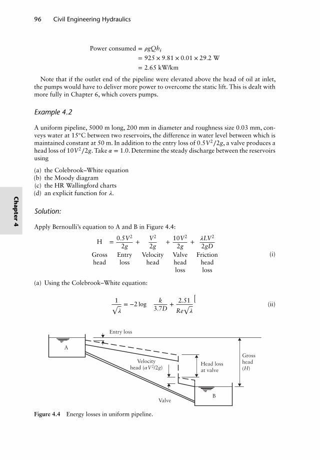
96 Civil Engineering Hydraulics
Power consumed = 𝜌gQhf
= 925 × 9.81 × 0.01 × 29.2 W
= 2.65 kW/km
Note that if the outlet end of the pipeline were elevated above the head of oil at inlet,the pumps would have to deliver more power to overcome the static lift. This is dealt withmore fully in Chapter 6, which covers pumps.
Example 4.2
A uniform pipeline, 5000 m long, 200 mm in diameter and roughness size 0.03 mm, con-veys water at 15◦C between two reservoirs, the difference in water level between which ismaintained constant at 50 m. In addition to the entry loss of 0.5V2∕2g, a valve produces ahead loss of 10V2∕2g. Take 𝛼 = 1.0. Determine the steady discharge between the reservoirsusing
(a) the Colebrook–White equation(b) the Moody diagram(c) the HR Wallingford charts(d) an explicit function for 𝜆.
Solution:
Apply Bernoulli’s equation to A and B in Figure 4.4:
H = 0.5V2
2g+ V2
2g+ 10V2
2g+ 𝜆LV2
2gDGross Entry Velocity Valve Frictionhead loss head head head
loss loss
(i)
(a) Using the Colebrook–White equation:
1√𝜆= −2 log
(k
3.7D+ 2.51
Re√𝜆
)(ii)
Valve
A
Entry loss
Head lossat valve
Grosshead(H)
B
Velocityhead (αV2/2g)
Figure 4.4 Energy losses in uniform pipeline.
Ch
apter
4
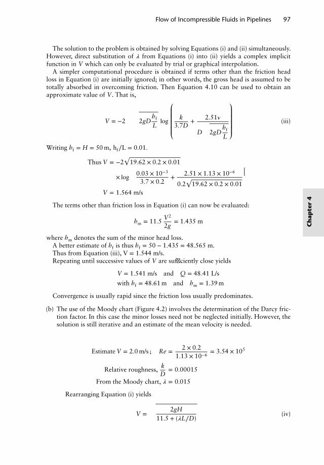
Flow of Incompressible Fluids in Pipelines 97
The solution to the problem is obtained by solving Equations (i) and (ii) simultaneously.However, direct substitution of 𝜆 from Equations (i) into (ii) yields a complex implicitfunction in V which can only be evaluated by trial or graphical interpolation.
A simpler computational procedure is obtained if terms other than the friction headloss in Equation (i) are initially ignored; in other words, the gross head is assumed to betotally absorbed in overcoming friction. Then Equation 4.10 can be used to obtain anapproximate value of V. That is,
V = −2
√2gD
hf
Llog
⎛⎜⎜⎜⎜⎝k
3.7D+ 2.51𝜈
D
√2gD
hf
L
⎞⎟⎟⎟⎟⎠(iii)
Writing hf = H = 50 m, hf∕L = 0.01.
Thus V = −2√
19.62 × 0.2 × 0.01
× log
(0.03 × 10⁻³
3.7 × 0.2+ 2.51 × 1.13 × 10−6
0.2√
19.62 × 0.2 × 0.01
)
V = 1.564 m/s
The terms other than friction loss in Equation (i) can now be evaluated:
hm = 11.5 V2
2g= 1.435 m
where hm denotes the sum of the minor head loss.A better estimate of hf is thus hf = 50 − 1.435 = 48.565 m.Thus from Equation (iii), V = 1.544 m/s.Repeating until successive values of V are sufficiently close yields
V = 1.541 m/s and Q = 48.41 L/s
with hf = 48.61 m and hm = 1.39 m
Convergence is usually rapid since the friction loss usually predominates.
(b) The use of the Moody chart (Figure 4.2) involves the determination of the Darcy fric-tion factor. In this case the minor losses need not be neglected initially. However, thesolution is still iterative and an estimate of the mean velocity is needed.
Estimate V = 2.0 m/s ; Re = 2 × 0.21.13 × 10−6
= 3.54 × 10⁵
Relative roughness, kD
= 0.00015
From the Moody chart, 𝜆 = 0.015
Rearranging Equation (i) yields
V =
√2gH
11.5 + (𝜆L∕D)(iv)
Ch
apte
r4
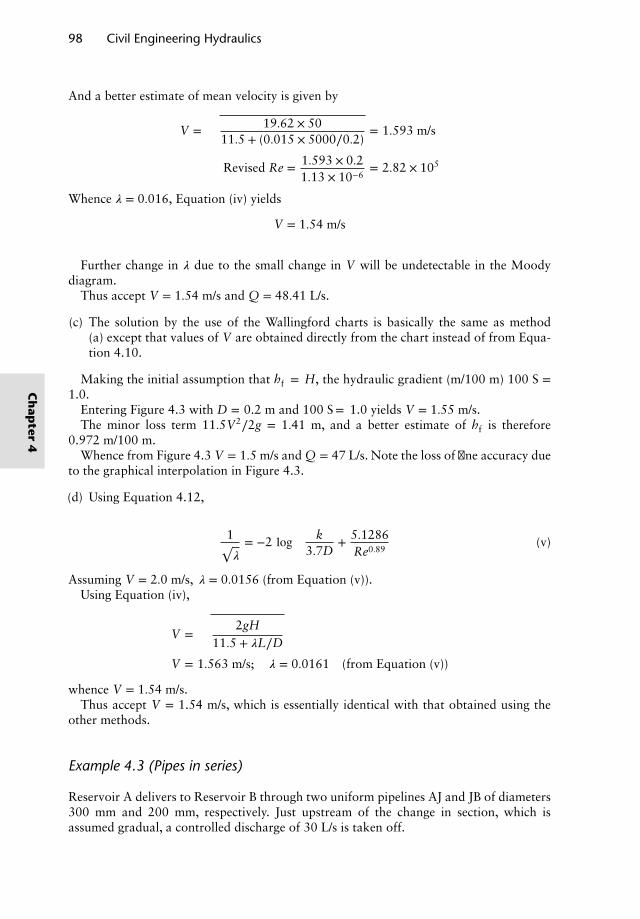
98 Civil Engineering Hydraulics
And a better estimate of mean velocity is given by
V =√
19.62 × 5011.5 + (0.015 × 5000∕0.2)
= 1.593 m/s
Revised Re = 1.593 × 0.21.13 × 10−6
= 2.82 × 10⁵
Whence 𝜆 = 0.016, Equation (iv) yields
V = 1.54 m/s
Further change in 𝜆 due to the small change in V will be undetectable in the Moodydiagram.
Thus accept V = 1.54 m/s and Q = 48.41 L/s.
(c) The solution by the use of the Wallingford charts is basically the same as method(a) except that values of V are obtained directly from the chart instead of from Equa-tion 4.10.
Making the initial assumption that hf = H, the hydraulic gradient (m/100 m) 100 S =1.0.
Entering Figure 4.3 with D = 0.2 m and 100 S= 1.0 yields V = 1.55 m/s.The minor loss term 11.5V2∕2g = 1.41 m, and a better estimate of hf is therefore
0.972 m/100 m.Whence from Figure 4.3 V = 1.5 m/s and Q = 47 L/s. Note the loss of fine accuracy due
to the graphical interpolation in Figure 4.3.
(d) Using Equation 4.12,
1√𝜆= −2 log
(k
3.7D+ 5.1286
Re0.89
)(v)
Assuming V = 2.0 m/s, 𝜆 = 0.0156 (from Equation (v)).Using Equation (iv),
V =
√2gH
11.5 + 𝜆L∕D
V = 1.563 m/s; 𝜆 = 0.0161 (from Equation (v))
whence V = 1.54 m/s.Thus accept V = 1.54 m/s, which is essentially identical with that obtained using the
other methods.
Example 4.3 (Pipes in series)
Reservoir A delivers to Reservoir B through two uniform pipelines AJ and JB of diameters300 mm and 200 mm, respectively. Just upstream of the change in section, which isassumed gradual, a controlled discharge of 30 L/s is taken off.
Ch
apter
4
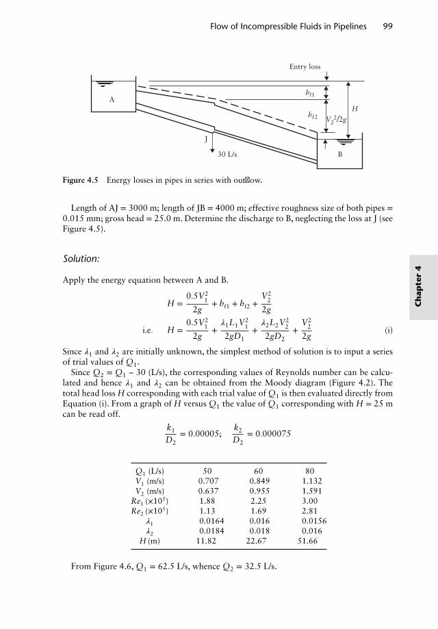
Flow of Incompressible Fluids in Pipelines 99
A
J
30 L/s
Entry loss
B
H
hf1
hf2 V22/2g
Figure 4.5 Energy losses in pipes in series with outflow.
Length of AJ = 3000 m; length of JB = 4000 m; effective roughness size of both pipes =0.015 mm; gross head = 25.0 m. Determine the discharge to B, neglecting the loss at J (seeFigure 4.5).
Solution:
Apply the energy equation between A and B.
H =0.5V2
1
2g+ hf1 + hf2 +
V22
2g
i.e. H =0.5V2
1
2g+𝜆1L1V2
1
2gD1+𝜆2L2V2
2
2gD2+
V22
2g(i)
Since 𝜆1 and 𝜆2 are initially unknown, the simplest method of solution is to input a seriesof trial values of Q1.
Since Q2 = Q1 – 30 (L/s), the corresponding values of Reynolds number can be calcu-lated and hence 𝜆1 and 𝜆2 can be obtained from the Moody diagram (Figure 4.2). Thetotal head loss H corresponding with each trial value of Q1 is then evaluated directly fromEquation (i). From a graph of H versus Q1 the value of Q1 corresponding with H = 25 mcan be read off.
k1
D2= 0.00005;
k2
D2= 0.000075
Q1 (L/s) 50 60 80V1 (m/s) 0.707 0.849 1.132V2 (m/s) 0.637 0.955 1.591
Re1 (×105) 1.88 2.25 3.00Re2 (×105) 1.13 1.69 2.81
𝜆1 0.0164 0.016 0.0156𝜆2 0.0184 0.018 0.016
H (m) 11.82 22.67 51.66
From Figure 4.6, Q1 = 62.5 L/s, whence Q2 = 32.5 L/s.
Ch
apte
r4
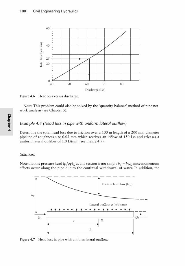
100 Civil Engineering Hydraulics
60
40
25
20
0
Tota
l hea
d lo
ss (
m)
40 50 60 70 80
Discharge (L/s)
Figure 4.6 Head loss versus discharge.
Note: This problem could also be solved by the ‘quantity balance’ method of pipe net-work analysis (see Chapter 5).
Example 4.4 (Head loss in pipe with uniform lateral outflow)
Determine the total head loss due to friction over a 100 m length of a 200 mm diameterpipeline of roughness size 0.03 mm which receives an inflow of 150 L/s and releases auniform lateral outflow of 1.0 L/(s m) (see Figure 4.7).
Solution:
Note that the pressure head (p∕𝜌g)X at any section is not simply h1 − hf,X since momentumeffects occur along the pipe due to the continual withdrawal of water. In addition, the
Friction head loss (hf,x)
Lateral outflow q (m3/(s m))
x
L
XQ1 Q2
h1
Figure 4.7 Head loss in pipe with uniform lateral outflow.
Ch
apter
4
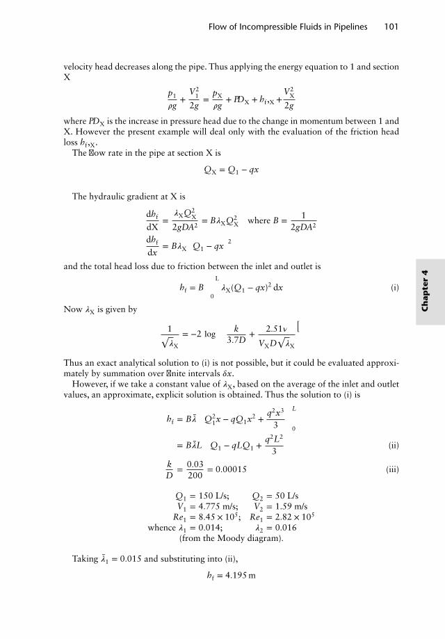
Flow of Incompressible Fluids in Pipelines 101
velocity head decreases along the pipe. Thus applying the energy equation to 1 and sectionX
p1
𝜌g+
V21
2g=
pX
𝜌g+ PDX + hf,X +
V2X
2g
where PDX is the increase in pressure head due to the change in momentum between 1 andX. However the present example will deal only with the evaluation of the friction headloss hf,X.
The flow rate in the pipe at section X is
QX = Q1 − qx
The hydraulic gradient at X is
dhf
dX=𝜆XQ2
X
2gDA2= B𝜆XQ2
X where B = 12gDA2
dhf
dx= B𝜆X
(Q1 − qx
)2
and the total head loss due to friction between the inlet and outlet is
hf = B∫L
0𝜆X(Q1 − qx)2 dx (i)
Now 𝜆X is given by
1√𝜆X
= −2 log
(k
3.7D+ 2.51𝜈
VXD√𝜆X
)
Thus an exact analytical solution to (i) is not possible, but it could be evaluated approxi-mately by summation over finite intervals 𝛿x.
However, if we take a constant value of 𝜆X, based on the average of the inlet and outletvalues, an approximate, explicit solution is obtained. Thus the solution to (i) is
hf = B��(
Q21x − qQ1x2 +
q2x3
3
)L
0
= B��L(
Q1 − qLQ1 +q2L2
3
)(ii)
kD
= 0.03200
= 0.00015 (iii)
Q1 = 150 L/s; Q2 = 50 L/sV1 = 4.775 m/s; V2 = 1.59 m/s
Re1 = 8.45 × 10⁵; Re1 = 2.82 × 10⁵
whence 𝜆1 = 0.014; 𝜆2 = 0.016(from the Moody diagram).
Taking ��1 = 0.015 and substituting into (ii),
hf = 4.195 m
Ch
apte
r4
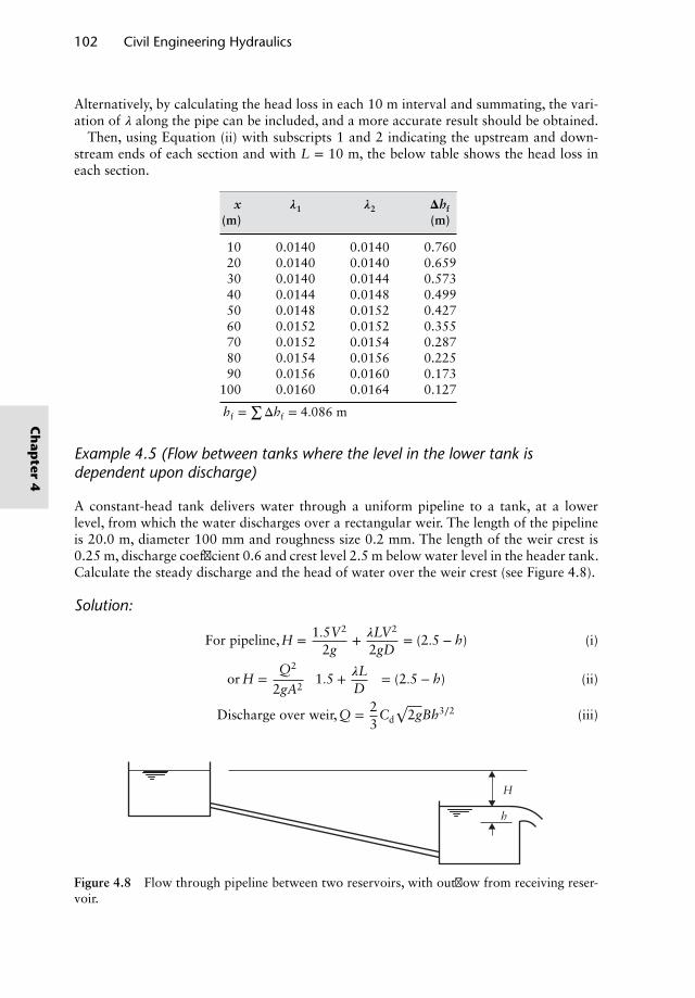
102 Civil Engineering Hydraulics
Alternatively, by calculating the head loss in each 10 m interval and summating, the vari-ation of 𝜆 along the pipe can be included, and a more accurate result should be obtained.
Then, using Equation (ii) with subscripts 1 and 2 indicating the upstream and down-stream ends of each section and with L = 10 m, the below table shows the head loss ineach section.
x 𝝀1 𝝀2 𝚫hf(m) (m)
10 0.0140 0.0140 0.76020 0.0140 0.0140 0.65930 0.0140 0.0144 0.57340 0.0144 0.0148 0.49950 0.0148 0.0152 0.42760 0.0152 0.0152 0.35570 0.0152 0.0154 0.28780 0.0154 0.0156 0.22590 0.0156 0.0160 0.173
100 0.0160 0.0164 0.127
hf =∑
Δhf = 4.086 m
Example 4.5 (Flow between tanks where the level in the lower tank isdependent upon discharge)
A constant-head tank delivers water through a uniform pipeline to a tank, at a lowerlevel, from which the water discharges over a rectangular weir. The length of the pipelineis 20.0 m, diameter 100 mm and roughness size 0.2 mm. The length of the weir crest is0.25 m, discharge coefficient 0.6 and crest level 2.5 m below water level in the header tank.Calculate the steady discharge and the head of water over the weir crest (see Figure 4.8).
Solution:
For pipeline,H = 1.5V2
2g+ 𝜆LV2
2gD= (2.5 − h) (i)
or H =Q2
2gA2
(1.5 + 𝜆L
D
)= (2.5 − h) (ii)
Discharge over weir,Q = 23
Cd
√2gBh3∕2 (iii)
H
h
Figure 4.8 Flow through pipeline between two reservoirs, with outflow from receiving reser-voir.
Ch
apter
4
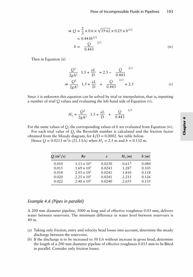
Flow of Incompressible Fluids in Pipelines 103
⇒ Q = 23× 0.6 ×
√19.62 × 0.25 × h3∕2
= 0.443h3∕2
h =(
Q0.443
)2∕3
(iv)
Then in Equation (ii)
Q2
2gA2
(1.5 + 𝜆L
D
)= 2.5 −
(Q
0.443
)2∕3
⇒Q2
2gA2
(1.5 + 𝜆L
D
)+(
Q0.443
)2∕3
= 2.5 (v)
Since 𝜆 is unknown this equation can be solved by trial or interpolation, that is, inputtinga number of trial Q values and evaluating the left-hand side of Equation (v):
H1 =Q2
2gA2
(1.5 + 𝜆L
D
)+(
Q0.443
)2∕3
For the same values of Q, the corresponding values of h are evaluated from Equation (iv).For each trial value of Q, the Reynolds number is calculated and the friction factor
obtained from the Moody diagram, for k∕D = 0.0002. See table below.Hence Q = 0.0213 m3/s (21.3 L/s) when H1 = 2.5 m and h = 0.132 m.
Q (m3∕s) Re 𝝀 H1 (m) h (m)
0.010 1.13 × 10⁵ 0.0250 0.617 0.0800.015 1.69 × 10⁵ 0.0243 1.287 0.1050.018 2.03 × 10⁵ 0.0241 1.810 0.1180.020 2.25 × 10⁵ 0.0241 2.215 0.1260.022 2.48 × 10⁵ 0.0240 2.655 0.135
Example 4.6 (Pipes in parallel)
A 200 mm diameter pipeline, 5000 m long and of effective roughness 0.03 mm, deliverswater between reservoirs. The minimum difference in water level between reservoirs is40 m.
(a) Taking only friction, entry and velocity head losses into account, determine the steadydischarge between the reservoirs.
(b) If the discharge is to be increased to 50 L/s without increase in gross head, determinethe length of a 200 mm diameter pipeline of effective roughness 0.015 mm to be fittedin parallel. Consider only friction losses.
Ch
apte
r4
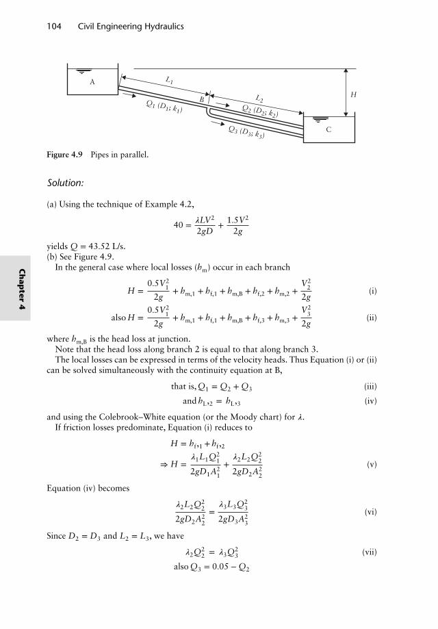
104 Civil Engineering Hydraulics
A
C
BQ2 (D2; k2)
Q1 (D1; k1)
Q3 (D3; k3)
L2
L1
H
Figure 4.9 Pipes in parallel.
Solution:
(a) Using the technique of Example 4.2,
40 = 𝜆LV2
2gD+ 1.5V2
2g
yields Q = 43.52 L/s.(b) See Figure 4.9.
In the general case where local losses (hm) occur in each branch
H =0.5V2
1
2g+ hm,1 + hf,1 + hm,B + hf,2 + hm,2 +
V22
2g(i)
also H =0.5V2
1
2g+ hm,1 + hf,1 + hm,B + hf,3 + hm,3 +
V23
2g(ii)
where hm,B is the head loss at junction.Note that the head loss along branch 2 is equal to that along branch 3.The local losses can be expressed in terms of the velocity heads. Thus Equation (i) or (ii)
can be solved simultaneously with the continuity equation at B,
that is,Q1 = Q2 + Q3 (iii)
and hL,2 = hL,3 (iv)
and using the Colebrook–White equation (or the Moody chart) for 𝜆.If friction losses predominate, Equation (i) reduces to
H = hf,1 +hf,2
⇒ H =𝜆1L1Q2
1
2gD1A21
+𝜆2L2Q2
2
2gD2A22
(v)
Equation (iv) becomes
𝜆2L2Q22
2gD2A22
=𝜆3L3Q2
3
2gD3A23
(vi)
Since D2 = D3 and L2 = L3, we have
𝜆2Q22 = 𝜆3Q2
3 (vii)
also Q3 = 0.05 − Q2
Ch
apter
4
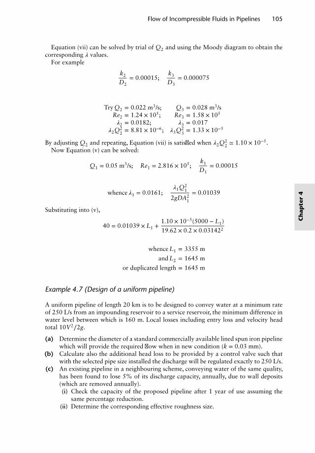
Flow of Incompressible Fluids in Pipelines 105
Equation (vii) can be solved by trial of Q2 and using the Moody diagram to obtain thecorresponding 𝜆 values.
For example
k2
D2= 0.00015;
k3
D3= 0.000075
Try Q2 = 0.022 m3/s; Q3 = 0.028 m3/sRe2 = 1.24 × 10⁵; Re3 = 1.58 × 10⁵
𝜆2 = 0.0182; 𝜆3 = 0.017𝜆2Q2
2 = 8.81 × 10⁻⁶; 𝜆3Q23 = 1.33 × 10⁻⁵
By adjusting Q2 and repeating, Equation (vii) is satisfied when 𝜆2Q22 ≃ 1.10 × 10⁻⁵.
Now Equation (v) can be solved:
Q1 = 0.05 m3/s; Re1 = 2.816 × 10⁵;k1
D1= 0.00015
whence 𝜆1 = 0.0161;𝜆1Q2
1
2gDA21
= 0.01039
Substituting into (v),
40 = 0.01039 × L1 +1.10 × 10⁻⁵(5000 − L1)
19.62 × 0.2 × 0.031422
whence L1 = 3355 m
and L2 = 1645 m
or duplicated length = 1645 m
Example 4.7 (Design of a uniform pipeline)
A uniform pipeline of length 20 km is to be designed to convey water at a minimum rateof 250 L/s from an impounding reservoir to a service reservoir, the minimum difference inwater level between which is 160 m. Local losses including entry loss and velocity headtotal 10V2∕2g.
(a) Determine the diameter of a standard commercially available lined spun iron pipelinewhich will provide the required flow when in new condition (k = 0.03 mm).
(b) Calculate also the additional head loss to be provided by a control valve such thatwith the selected pipe size installed the discharge will be regulated exactly to 250 L/s.
(c) An existing pipeline in a neighbouring scheme, conveying water of the same quality,has been found to lose 5% of its discharge capacity, annually, due to wall deposits(which are removed annually).(i) Check the capacity of the proposed pipeline after 1 year of use assuming the
same percentage reduction.(ii) Determine the corresponding effective roughness size.
Ch
apte
r4
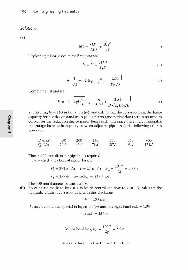
106 Civil Engineering Hydraulics
Solution:
(a)
160 = 𝜆LV2
2gD+ 10V2
2g(i)
Neglecting minor losses in the first instance,
hf = H = 𝜆LV2
2gD(ii)
⇒1√𝜆= −2 log
(k
3.7D+ 2.51
Re√𝜆
)(iii)
Combining (ii) and (iii),
V = −2
√2gD
hf
Llog
(k
3.7D+ 2.51𝜈
D√
2gDhf∕L
)(iv)
Substituting hf = 160 in Equation (iv), and calculating the corresponding dischargecapacity for a series of standard pipe diameters (and noting that there is no need tocorrect for the reduction due to minor losses each time since there is a considerablepercentage increase in capacity between adjacent pipe sizes), the following table isproduced:
D (mm) 150 200 250 300 350 400Q (L/s) 20.3 43.6 78.6 127.3 191.1 271.5
Thus a 400 mm diameter pipeline is required.Now check the effect of minor losses:
Q = 271.5 L/s; V = 2.16 m/s; hm = 10V2
2g= 2.38 m
hf = 157.6; revised Q = 269.4 L/s
The 400 mm diameter is satisfactory.(b) To calculate the head loss at a valve to control the flow to 250 L/s, calculate the
hydraulic gradient corresponding with this discharge:
V = 1.99 m/s
hf may be obtained by trial in Equation (iv) until the right-hand side = 1.99
Thus hf = 137 m
Minor head loss, hm = 10V2
2g= 2.0 m
Thus valve loss = 160 − 137 − 2.0 = 21.0 m
Ch
apter
4
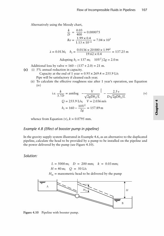
Flow of Incompressible Fluids in Pipelines 107
Alternatively using the Moody chart,
kD
= 0.03400
= 0.000075
Re = 1.99 × 0.41.13 × 10−6
= 7.04 × 10⁵
𝜆 = 0.0136; hf =0.0136 × 20 000 × 1.992
19.62 × 0.4= 137.25 m
Adopting hf = 137 m; 10V2∕2g = 2.0 m
Additional loss by valve = 160 − (137 + 2.0) = 21 m.(c) (i) 5% annual reduction in capacity.
Capacity at the end of 1 year = 0.95 × 269.4 = 255.9 L/sPipe will be satisfactory if cleaned each year.
(ii) To calculate the effective roughness size after 1 year’s operation, use Equation(iv)
i.e. k3.7D
= antilog
(− V√
2gDhf∕L
)− 2.5 𝜈
D√
2gDhf∕L(v)
Q = 255.9 L/s; V = 2.036 m/s
hf = 160 − 10V2
2g= 157.89 m
whence from Equation (v), k = 0.0795 mm.
Example 4.8 (Effect of booster pump in pipeline)
In the gravity supply system illustrated in Example 4.6, as an alternative to the duplicatedpipeline, calculate the head to be provided by a pump to be installed on the pipeline andthe power delivered by the pump (see Figure 4.10).
Solution:
L = 5000 m; D = 200 mm; k = 0.03 mm;
H = 40 m; Q = 50 L/s
Hm = manometric head to be delivered by the pump
HHm
B
A
Figure 4.10 Pipeline with booster pump.
Ch
apte
r4
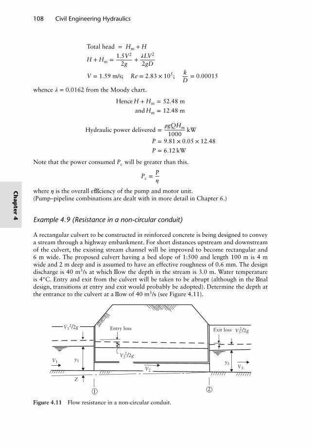
108 Civil Engineering Hydraulics
Total head = Hm + H
H + Hm = 1.5V2
2g+ 𝜆LV2
2gD
V = 1.59 m/s; Re = 2.83 × 10⁵; kD
= 0.00015
whence 𝜆 = 0.0162 from the Moody chart.
Hence H + Hm = 52.48 m
and Hm = 12.48 m
Hydraulic power delivered =𝜌gQHm
1000kW
P = 9.81 × 0.05 × 12.48
P = 6.12 kW
Note that the power consumed Pc will be greater than this.
Pc =P𝜂
where 𝜂 is the overall efficiency of the pump and motor unit.(Pump–pipeline combinations are dealt with in more detail in Chapter 6.)
Example 4.9 (Resistance in a non-circular conduit)
A rectangular culvert to be constructed in reinforced concrete is being designed to conveya stream through a highway embankment. For short distances upstream and downstreamof the culvert, the existing stream channel will be improved to become rectangular and6 m wide. The proposed culvert having a bed slope of 1:500 and length 100 m is 4 mwide and 2 m deep and is assumed to have an effective roughness of 0.6 mm. The designdischarge is 40 m3/s at which flow the depth in the stream is 3.0 m. Water temperatureis 4◦C. Entry and exit from the culvert will be taken to be abrupt (although in the finaldesign, transitions at entry and exit would probably be adopted). Determine the depth atthe entrance to the culvert at a flow of 40 m3/s (see Figure 4.11).
Entry loss Exit loss
1 2
Z
V1
V2V3
V32/2g
V22/2g
V12/2g
y1 y3
Figure 4.11 Flow resistance in a non-circular conduit.
Ch
apter
4
Flow of Incompressible Fluids in Pipelines 109
Solution:
Referring to Figure 4.11, apply the energy equation to 1 and 2
Z + y1 +V2
1
2g= y3 +
V23
2g+ entry loss + friction loss in culvert + exit loss (i)
The entry loss coefficient Kc may be less than 0.5, which is commonly adopted for entryfrom a reservoir. Assuming that the loss at the contraction is similar to that for concentricpipes, Kc will depend on the ratio of upstream and downstream areas of flow, derived fromthe table in Section 4.3 as follows:
A2∕A1 0.00 0.04 0.16 0.36 1.00Kc 0.50 0.45 0.38 0.28 0.00
Assume y1 = 4.0 m, then A2∕A1 = 8∕24 = 0.3;whence Kc = 0.3.
Discharge = 40.0 m3/s; V2 = 408
= 5.0 m/s
Entry loss = 0.3V2
2
2g= 0.38 m
The exit loss (expansion) is expressed as (V2 − V3)2∕2g.
V3 = 4080
= 2.22 m/s whence exit loss = 0.39 m
Friction head loss in culvert: referring to Section 4.2, the resistance in the duct can becalculated by ‘transforming’ the cross section into an equivalent circular section by equat-ing the hydraulic radii. For the culvert, R = A∕P = 8∕12 m and the equivalent diameterDe is therefore 2.67 m (=4R).
Note that either the Colebrook–White equation 4.9 or its graphical form (Figure 4.2)can now be used with D = 2.67 m.
Kinematic viscosity of water at 4◦C = 1.568 × 10⁻⁶ m2/s
V2 = 5 m/s; Re = 5 × 2.671.568 × 10−6
= 8.5 × 10⁶
kD
= 0.6 × 10⁻³
2.67= 0.000225
From the Moody chart, 𝜆 = 0.014.
hf =0.014 × 100 × 52
19.62 × 2.67= 0.668 m (say 0.67 m)
V23
2g= 2.222
19.62= 0.25 m
Ch
apte
r4
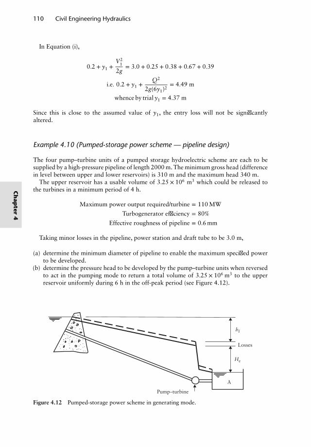
110 Civil Engineering Hydraulics
In Equation (i),
0.2 + y1 +V2
1
2g= 3.0 + 0.25 + 0.38 + 0.67 + 0.39
i.e. 0.2 + y1 +Q2
2g(6y1)2= 4.49 m
whence by trial y1 = 4.37 m
Since this is close to the assumed value of y1, the entry loss will not be significantlyaltered.
Example 4.10 (Pumped-storage power scheme — pipeline design)
The four pump–turbine units of a pumped storage hydroelectric scheme are each to besupplied by a high-pressure pipeline of length 2000 m. The minimum gross head (differencein level between upper and lower reservoirs) is 310 m and the maximum head 340 m.
The upper reservoir has a usable volume of 3.25 × 10⁶ m3 which could be released tothe turbines in a minimum period of 4 h.
Maximum power output required/turbine = 110 MW
Turbogenerator efficiency = 80%Effective roughness of pipeline = 0.6 mm
Taking minor losses in the pipeline, power station and draft tube to be 3.0 m,
(a) determine the minimum diameter of pipeline to enable the maximum specified powerto be developed.
(b) determine the pressure head to be developed by the pump–turbine units when reversedto act in the pumping mode to return a total volume of 3.25 × 10⁶ m3 to the upperreservoir uniformly during 6 h in the off-peak period (see Figure 4.12).
Pump–turbine
Losses
hf
He
A
Figure 4.12 Pumped-storage power scheme in generating mode.
Ch
apter
4
Flow of Incompressible Fluids in Pipelines 111
Solution:
(a) Pipe capacity must be adequate to convey the required flow under minimum headconditions:
Qmax
unit= 3.25 × 10⁶
4 × 4 × 3600= 56.42 m3/s
Power generated, P =efficiency × 𝜌gQHe
106MW = 110 MW
where He is the effective head at the turbines.
⇒ 110 =0.8 × 1000 × 9.81 × 56.42 × He
106
whence He = 248 m
Total head loss = 310 − 248 = 62 m
Head loss due to friction = 62 − minor losses = 62 − 3.0 = 59 m
hf =𝜆LV2
2gDand 1√
𝜆= −2 log
(k
3.7D+ 2.51
Re√𝜆
)
Since the hydraulic gradient is known but D is unknown, it is preferable to use Equation4.10 in this case rather than use the Moody chart. That is,
V = −2
√2gD
hf
Llog
(k
3.7D+ 251𝜈
D√
2gDhf∕L
)
and Q = 𝜋D2V4
Substituting values of D yields the corresponding discharge under the available hydraulicgradient.
D (m) 1.0 2.0 2.5 2.6 2.65Q (m3/s) 4.47 27.32 48.87 54.123 56.875
Hence required diameter = 2.65 m.
(b) In pumping mode, static lift = 340 m
Q = 3.25 × 10⁶
6 × 4 × 3600= 37.616 m3/s
Ch
apte
r4
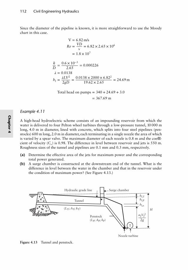
112 Civil Engineering Hydraulics
Since the diameter of the pipeline is known, it is more straighforward to use the Moodychart in this case.
V = 6.82 m/s
Re = VD𝜈
= 6.82 × 2.65 × 106
= 1.8 × 10⁷
kD
= 0.6 × 10⁻³
2.65= 0.000226
𝜆 = 0.0138
hf =𝜆LV2
2gD= 0.0138 × 2000 × 6.822
19.62 × 2.65= 24.69 m
Total head on pumps = 340 + 24.69 + 3.0
= 367.69 m
Example 4.11
A high-head hydroelectric scheme consists of an impounding reservoir from which thewater is delivered to four Pelton wheel turbines through a low-pressure tunnel, 10 000 mlong, 4.0 m in diameter, lined with concrete, which splits into four steel pipelines (pen-stocks) 600 m long, 2.0 m in diameter, each terminating in a single nozzle the area of whichis varied by a spear valve. The maximum diameter of each nozzle is 0.8 m and the coeffi-cient of velocity (Cv) is 0.98. The difference in level between reservoir and jets is 550 m.Roughness sizes of the tunnel and pipelines are 0.1 mm and 0.3 mm, respectively.
(a) Determine the effective area of the jets for maximum power and the correspondingtotal power generated.
(b) A surge chamber is constructed at the downstream end of the tunnel. What is thedifference in level between the water in the chamber and that in the reservoir underthe condition of maximum power? (See Figure 4.13.)
Hydraulic grade line Surge chamber
2g
hf,Thf,P
hl,n
αJVJ2
T
H
Tunnel
(LT; AT; kT)
(LP; AP; kP)
Nozzle turbine
Penstock
Figure 4.13 Tunnel and penstock.
Ch
apter
4
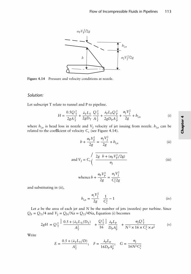
Flow of Incompressible Fluids in Pipelines 113
hl,n
h
αPVP2/2g
αJVJ2/2g
Figure 4.14 Pressure and velocity conditions at nozzle.
Solution:
Let subscript T relate to tunnel and P to pipeline.
H =0.5Q 2
T
2gA 2T
+𝜆TLT
2gDT
Q 2T
A 2T
+𝜆PLPQ 2
P
2gDPA 2P
+𝛼JV
2J
2g+ hl,n (i)
where hl,n is head loss in nozzle and VJ velocity of jet issuing from nozzle. hl,n can berelated to the coefficient of velocity Cv (see Figure 4.14).
h +𝛼PV2
P
2g=𝛼JV
2J
2g+ hl,n (ii)
and VJ = Cv
√√√√2g(h + (𝛼PV2
P∕2g))
𝛼J(iii)
whence h +𝛼PV2
P
2g=𝛼JV
2J
C2v2g
and substituting in (ii),
hl,n =𝛼jV
2J
2g
(1
C2v
− 1)
(iv)
Let a be the area of each jet and N be the number of jets (nozzles) per turbine. SinceQP = QT∕4 and VJ = QP∕Na = QT∕4Na, Equation (i) becomes
2gH = Q 2T
[0.5 + (𝜆TLT∕DT)
A2T
]+
Q 2T
16
[𝜆PLP
DPA2P
]+
𝛼JQ2T
N 2 × 16 × C2v × a2
(v)
Write
E =0.5 + (𝜆TLT∕D)
A2T
; F =𝜆PLP
16DPA2P
; G =𝛼J
16N2C2v
Ch
apte
r4
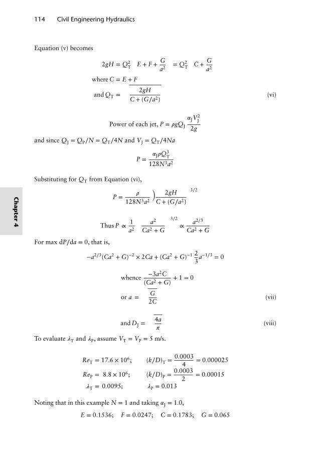
114 Civil Engineering Hydraulics
Equation (v) becomes
2gH = Q2T
(E + F + G
a2
)= Q2
T
(C + G
a2
)where C = E + F
and QT =
√2gH
C + (G∕a2)(vi)
Power of each jet, P = 𝜌gQJ
𝛼JV2J
2g
and since QJ = QP∕N = QT∕4N and VJ = QT∕4Na
P =𝛼J𝜌Q
3T
128N3a2
Substituting for QT from Equation (vi),
P = 𝜌
128N3a2
[2gH
C + (G∕a2)
]3∕2
Thus P ∝ 1a2
(a2
Ca2 + G
)3∕2
∝ a2∕3
Ca2 + G
For max dP∕da = 0, that is,
−a2∕3(Ca2 + G)−2 × 2Ca + (Ca2 + G)−1 23
a−1∕3 = 0
whence −3a2C(Ca2 + G)
+ 1 = 0
or a =√
G2C
(vii)
and DJ =√
4a𝜋
(viii)
To evaluate 𝜆T and 𝜆P, assume VT = VP = 5 m/s.
ReT = 17.6 × 10⁶; (k∕D)T = 0.00034
= 0.000025
ReP = 8.8 × 10⁶; (k∕D)P = 0.00032
= 0.00015
𝜆T = 0.0095; 𝜆P = 0.013
Noting that in this example N = 1 and taking 𝛼J = 1.0,
E = 0.1536; F = 0.0247; C = 0.1783; G = 0.065
Ch
apter
4
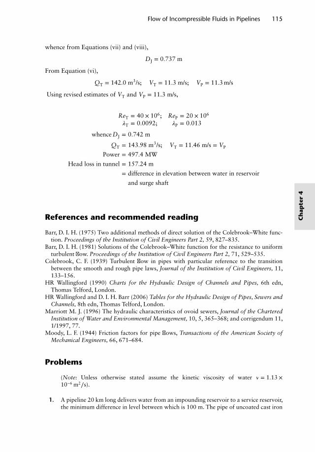
Flow of Incompressible Fluids in Pipelines 115
whence from Equations (vii) and (viii),
DJ = 0.737 m
From Equation (vi),
QT = 142.0 m3/s; VT = 11.3 m/s; VP = 11.3 m/s
Using revised estimates of VT and VP = 11.3 m/s,
ReT = 40 × 106; ReP = 20 × 106
𝜆T = 0.0092; 𝜆P = 0.013
whence DJ = 0.742 m
QT = 143.98 m3/s; VT = 11.46 m/s = VP
Power = 497.4 MW
Head loss in tunnel = 157.24 m
= difference in elevation between water in reservoir
and surge shaft
References and recommended reading
Barr, D. I. H. (1975) Two additional methods of direct solution of the Colebrook–White func-tion. Proceedings of the Institution of Civil Engineers Part 2, 59, 827–835.
Barr, D. I. H. (1981) Solutions of the Colebrook–White function for the resistance to uniformturbulent flow. Proceedings of the Institution of Civil Engineers Part 2, 71, 529–535.
Colebrook, C. F. (1939) Turbulent flow in pipes with particular reference to the transitionbetween the smooth and rough pipe laws, Journal of the Institution of Civil Engineers, 11,133–156.
HR Wallingford (1990) Charts for the Hydraulic Design of Channels and Pipes, 6th edn,Thomas Telford, London.
HR Wallingford and D. I. H. Barr (2006) Tables for the Hydraulic Design of Pipes, Sewers andChannels, 8th edn, Thomas Telford, London.
Marriott M. J. (1996) The hydraulic characteristics of ovoid sewers, Journal of the CharteredInstitution of Water and Environmental Management, 10, 5, 365–368; and corrigendum 11,1/1997, 77.
Moody, L. F. (1944) Friction factors for pipe flows, Transactions of the American Society ofMechanical Engineers, 66, 671–684.
Problems
(Note: Unless otherwise stated assume the kinetic viscosity of water 𝜈 = 1.13 ×10⁻⁶ m2∕s).
1. A pipeline 20 km long delivers water from an impounding reservoir to a service reservoir,the minimum difference in level between which is 100 m. The pipe of uncoated cast iron
Ch
apte
r4
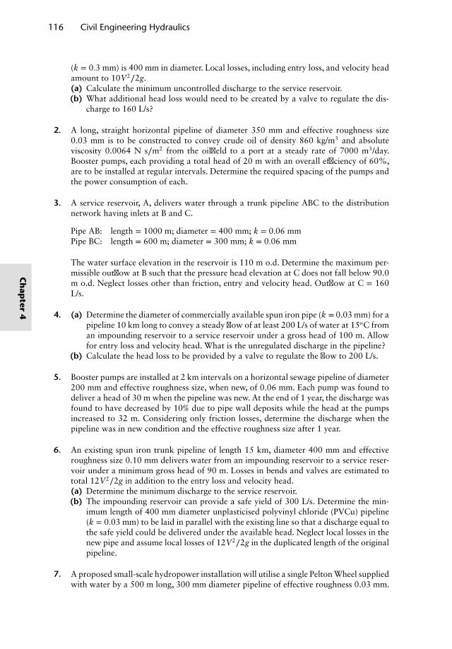
116 Civil Engineering Hydraulics
(k = 0.3 mm) is 400 mm in diameter. Local losses, including entry loss, and velocity headamount to 10V2∕2g.(a) Calculate the minimum uncontrolled discharge to the service reservoir.(b) What additional head loss would need to be created by a valve to regulate the dis-
charge to 160 L/s?
2. A long, straight horizontal pipeline of diameter 350 mm and effective roughness size0.03 mm is to be constructed to convey crude oil of density 860 kg/m3 and absoluteviscosity 0.0064 N s∕m2 from the oilfield to a port at a steady rate of 7000 m3/day.Booster pumps, each providing a total head of 20 m with an overall efficiency of 60%,are to be installed at regular intervals. Determine the required spacing of the pumps andthe power consumption of each.
3. A service reservoir, A, delivers water through a trunk pipeline ABC to the distributionnetwork having inlets at B and C.
Pipe AB: length = 1000 m; diameter = 400 mm; k = 0.06 mmPipe BC: length = 600 m; diameter = 300 mm; k = 0.06 mm
The water surface elevation in the reservoir is 110 m o.d. Determine the maximum per-missible outflow at B such that the pressure head elevation at C does not fall below 90.0m o.d. Neglect losses other than friction, entry and velocity head. Outflow at C = 160L/s.
4. (a) Determine the diameter of commercially available spun iron pipe (k = 0.03 mm) for apipeline 10 km long to convey a steady flow of at least 200 L/s of water at 15oC froman impounding reservoir to a service reservoir under a gross head of 100 m. Allowfor entry loss and velocity head. What is the unregulated discharge in the pipeline?
(b) Calculate the head loss to be provided by a valve to regulate the flow to 200 L/s.
5. Booster pumps are installed at 2 km intervals on a horizontal sewage pipeline of diameter200 mm and effective roughness size, when new, of 0.06 mm. Each pump was found todeliver a head of 30 m when the pipeline was new. At the end of 1 year, the discharge wasfound to have decreased by 10% due to pipe wall deposits while the head at the pumpsincreased to 32 m. Considering only friction losses, determine the discharge when thepipeline was in new condition and the effective roughness size after 1 year.
6. An existing spun iron trunk pipeline of length 15 km, diameter 400 mm and effectiveroughness size 0.10 mm delivers water from an impounding reservoir to a service reser-voir under a minimum gross head of 90 m. Losses in bends and valves are estimated tototal 12V2∕2g in addition to the entry loss and velocity head.(a) Determine the minimum discharge to the service reservoir.(b) The impounding reservoir can provide a safe yield of 300 L/s. Determine the min-
imum length of 400 mm diameter unplasticised polyvinyl chloride (PVCu) pipeline(k = 0.03 mm) to be laid in parallel with the existing line so that a discharge equal tothe safe yield could be delivered under the available head. Neglect local losses in thenew pipe and assume local losses of 12V2∕2g in the duplicated length of the originalpipeline.
7. A proposed small-scale hydropower installation will utilise a single Pelton Wheel suppliedwith water by a 500 m long, 300 mm diameter pipeline of effective roughness 0.03 mm.
Ch
apter
4
Flow of Incompressible Fluids in Pipelines 117
The pipeline terminates in a nozzle (Cv = 0.98) which is 15 m below the level in thereservoir. Determine the nozzle diameter such that the jet will have the maximum possiblepower using the available head, and determine the jet power.
8. Oil of absolute viscosity 0.07 N s/m2 and density 925 kg/m3 is to be pumped by a roto-dynamic pump along a uniform pipeline 500 m long to discharge to atmosphere at anelevation of +80 m o.d. The pressure head elevation at the pump delivery is 95 m o.d.Neglecting minor losses, compare the discharges attained when the pipe of roughness0.06 mm is (a) 100 mm and (b) 150 mm diameter, and state in each whether the flow islaminar or turbulent.
9. A pipeline 10 km long is to be designed to deliver water from a river through a pumpingstation to the inlet tank of a treatment works. Elevation of delivery pressure head at thepumping station is 50 m o.d.; elevation of water in tank is 30 m o.d. Neglecting minorlosses, compare the discharges obtainable using(a) a 300 mm diameter plastic pipeline which may be considered to be smooth
(i) using the Colebrook–White equation(ii) using the Blasius equation
(b) a 300 mm diameter pipeline with an effective roughness of 0.6 mm(i) using the Karman–Prandtl rough law(ii) using the Colebrook–White equation.
10. Determine the hydraulic gradient in a rectangular concrete culvert 1 m wide and 0.6m high of roughness size 0.06 mm when running full and conveying water at a rate of2.5 m3/s. C
hap
ter
4

Chapter 5Pipe Network Analysis
5.1 Introduction
Water distribution network analysis provides the basis for the design of new systems andthe extension of existing systems. Design criteria are that specified minimum flow ratesand pressure heads must be attained at the outflow points of the network. The flow andpressure distributions across a network are affected by the arrangement and sizes of thepipes and the distribution of the outflows. Since a change of diameter in one pipe lengthwill affect the flow and pressure distribution everywhere, network design is not an explicitprocess. Optimal design methods almost invariably incorporate the hydraulic analysis ofthe system in which the pipe diameters are systematically altered (see e.g. Featherstone andEl Jumailly, 1983).
Pipe network analysis involves the determination of the pipe flow rates and pressureheads which satisfy the continuity and energy conservation equations. These may be statedas follows:
(i) Continuity: The algebraic sum of the flow rates in the pipes meeting at a junction,together with any external flows, is zero:
I=NP(J)∑I=1
QIJ − FJ = 0, J = 1, NJ [5.1]
in which QIJ is the flow rate in pipe IJ at junction J, NP(J) the number of pipesmeeting at junction J, FJ the external flow rate (outflow) at J and NJ the total numberof junctions in the network.
(ii) Energy conservation: The algebraic sum of the head losses in the pipes, together withany heads generated by inline booster pumps, around any closed loop formed bypipes is zero.
J=NP (I)∑J=1
hL,IJ − Hm,IJ = 0, I = 1, NL [5.2]
Nalluri & Featherstone’s Civil Engineering Hydraulics: Essential Theory with Worked Examples,Sixth Edition. Martin Marriott.© 2016 John Wiley & Sons, Ltd. Published 2016 by John Wiley & Sons, Ltd.Companion Website: www.wiley.com/go/Marriott
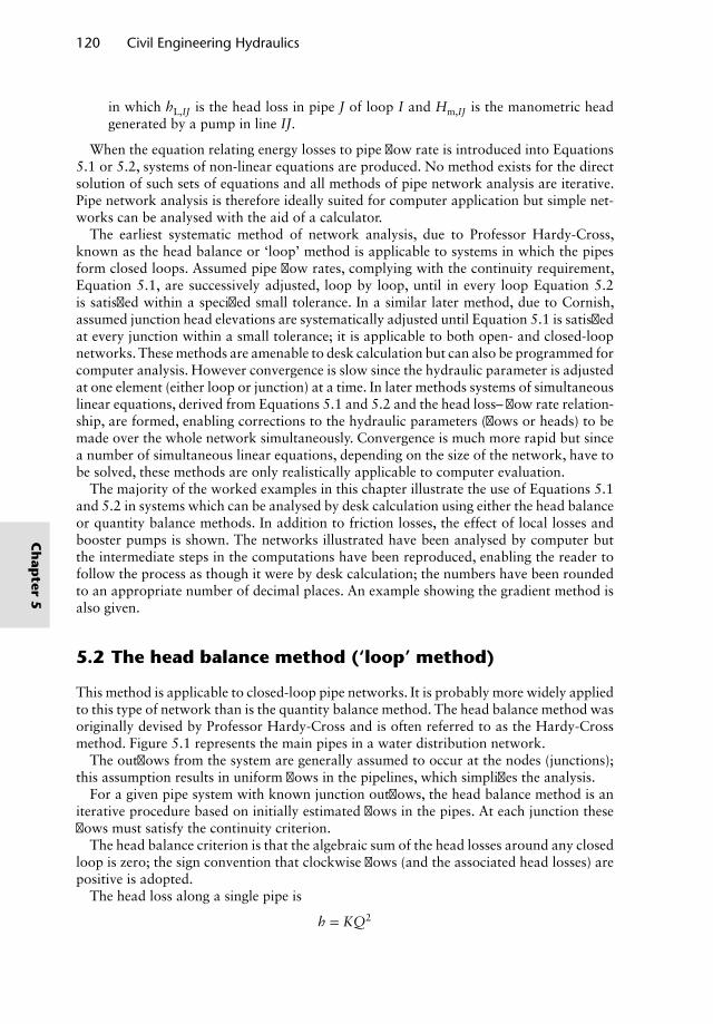
120 Civil Engineering Hydraulics
in which hL,IJ is the head loss in pipe J of loop I and Hm,IJ is the manometric headgenerated by a pump in line IJ.
When the equation relating energy losses to pipe flow rate is introduced into Equations5.1 or 5.2, systems of non-linear equations are produced. No method exists for the directsolution of such sets of equations and all methods of pipe network analysis are iterative.Pipe network analysis is therefore ideally suited for computer application but simple net-works can be analysed with the aid of a calculator.
The earliest systematic method of network analysis, due to Professor Hardy-Cross,known as the head balance or ‘loop’ method is applicable to systems in which the pipesform closed loops. Assumed pipe flow rates, complying with the continuity requirement,Equation 5.1, are successively adjusted, loop by loop, until in every loop Equation 5.2is satisfied within a specified small tolerance. In a similar later method, due to Cornish,assumed junction head elevations are systematically adjusted until Equation 5.1 is satisfiedat every junction within a small tolerance; it is applicable to both open- and closed-loopnetworks. These methods are amenable to desk calculation but can also be programmed forcomputer analysis. However convergence is slow since the hydraulic parameter is adjustedat one element (either loop or junction) at a time. In later methods systems of simultaneouslinear equations, derived from Equations 5.1 and 5.2 and the head loss– flow rate relation-ship, are formed, enabling corrections to the hydraulic parameters (flows or heads) to bemade over the whole network simultaneously. Convergence is much more rapid but sincea number of simultaneous linear equations, depending on the size of the network, have tobe solved, these methods are only realistically applicable to computer evaluation.
The majority of the worked examples in this chapter illustrate the use of Equations 5.1and 5.2 in systems which can be analysed by desk calculation using either the head balanceor quantity balance methods. In addition to friction losses, the effect of local losses andbooster pumps is shown. The networks illustrated have been analysed by computer butthe intermediate steps in the computations have been reproduced, enabling the reader tofollow the process as though it were by desk calculation; the numbers have been roundedto an appropriate number of decimal places. An example showing the gradient method isalso given.
5.2 The head balance method (‘loop’ method)
This method is applicable to closed-loop pipe networks. It is probably more widely appliedto this type of network than is the quantity balance method. The head balance method wasoriginally devised by Professor Hardy-Cross and is often referred to as the Hardy-Crossmethod. Figure 5.1 represents the main pipes in a water distribution network.
The outflows from the system are generally assumed to occur at the nodes (junctions);this assumption results in uniform flows in the pipelines, which simplifies the analysis.
For a given pipe system with known junction outflows, the head balance method is aniterative procedure based on initially estimated flows in the pipes. At each junction theseflows must satisfy the continuity criterion.
The head balance criterion is that the algebraic sum of the head losses around any closedloop is zero; the sign convention that clockwise flows (and the associated head losses) arepositive is adopted.
The head loss along a single pipe is
h = KQ2
Ch
apter
5
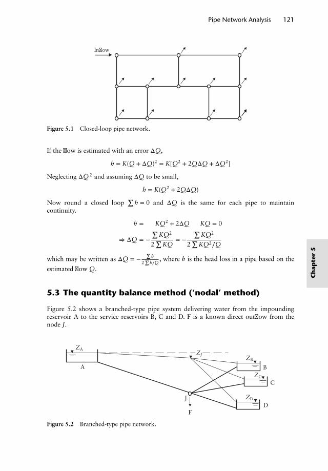
Pipe Network Analysis 121
Inflow
Figure 5.1 Closed-loop pipe network.
If the flow is estimated with an error ΔQ,
h = K(Q + ΔQ)2 = K[Q2 + 2QΔQ + ΔQ2]
Neglecting ΔQ2 and assuming ΔQ to be small,
h = K(Q2 + 2QΔQ)
Now round a closed loop∑
h = 0 and ΔQ is the same for each pipe to maintaincontinuity. ∑
h =∑
KQ2 + 2ΔQ∑
KQ = 0
⇒ ΔQ = −∑
KQ2
2∑
KQ= −
∑KQ2
2∑
KQ2∕Q
which may be written as ΔQ = −∑
h
2∑
h∕Q, where h is the head loss in a pipe based on the
estimated flow Q.
5.3 The quantity balance method (‘nodal’ method)
Figure 5.2 shows a branched-type pipe system delivering water from the impoundingreservoir A to the service reservoirs B, C and D. F is a known direct outflow from thenode J.
C
D
B
ZB
ZA
ZC
J
F
A
ZD
ZJ
Figure 5.2 Branched-type pipe network.
Ch
apte
r5
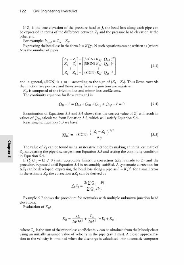
122 Civil Engineering Hydraulics
If ZJ is the true elevation of the pressure head at J, the head loss along each pipe canbe expressed in terms of the difference between ZJ and the pressure head elevation at theother end.
For example: hL,AJ = ZA − ZJ.Expressing the head loss in the form h = KQ2, N such equations can be written as (where
N is the number of pipes)
⎡⎢⎢⎢⎣ZA − ZJZB − ZJ
⋮ZI − ZJ
⎤⎥⎥⎥⎦==
=
⎡⎢⎢⎢⎣(SIGN) KAJ(|QAJ|)2
(SIGN) KBJ(|QBJ|)2
⋮(SIGN) KIJ(|QIJ|)2
⎤⎥⎥⎥⎦[5.3]
and in general, (SIGN) is + or − according to the sign of (ZI − ZJ). Thus flows towardsthe junction are positive and flows away from the junction are negative.
KIJ is composed of the friction loss and minor loss coefficients.The continuity equation for flow rates at J is
∑QIJ − F = QAJ + QBJ + QCJ + QDJ − F = 0 [5.4]
Examination of Equations 5.3 and 5.4 shows that the correct value of ZJ will result invalues of QIJ, calculated from Equation 5.3, which will satisfy Equation 5.4.
Rearranging Equation 5.3 we have
[QIJ] =
[(SIGN)
(|ZI − ZJ|KIJ
)1∕2][5.5]
The value of ZJ can be found using an iterative method by making an initial estimate ofZJ, calculating the pipe discharges from Equation 5.5 and testing the continuity conditionin Equation 5.4.
If (∑
QIJ − E) ≠ 0 (with acceptable limits), a correction ΔZJ is made to ZJ and theprocedure repeated until Equation 5.4 is reasonably satisfied. A systematic correction forΔZJ can be developed: expressing the head loss along a pipe as h = KQ2, for a small errorin the estimate ZJ, the correction ΔZJ can be derived as
△ZJ =2(∑
QIJ − F)∑QIJ∕hIJ
Example 5.7 shows the procedure for networks with multiple unknown junction headelevations.
Evaluation of KIJ:
KIJ =𝜆L
2gDA2+
Cm
2gA2(=Kf + Km)
where Cm is the sum of the minor loss coefficients.𝜆 can be obtained from the Moody chartusing an initially assumed value of velocity in the pipe (say 1 m/s). A closer approxima-tion to the velocity is obtained when the discharge is calculated. For automatic computer
Ch
apter
5
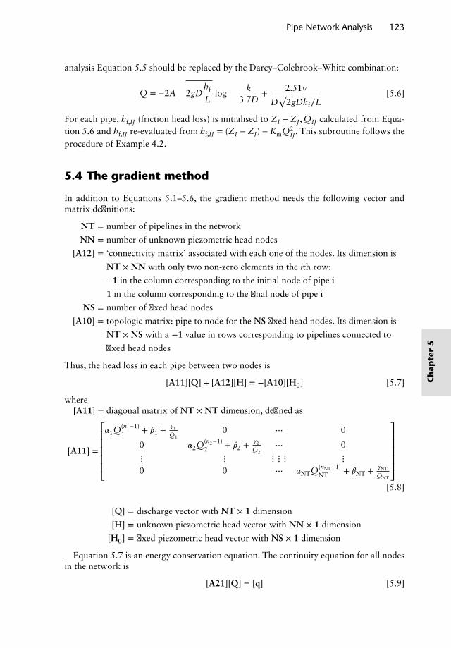
Pipe Network Analysis 123
analysis Equation 5.5 should be replaced by the Darcy–Colebrook–White combination:
Q = −2A
√2gD
hf
Llog
(k
3.7D+ 2.51𝜈
D√
2gDhf∕L
)[5.6]
For each pipe, hf,IJ (friction head loss) is initialised to ZI − ZJ, QIJ calculated from Equa-tion 5.6 and hf,IJ re-evaluated from hf,IJ = (ZI − ZJ) − KmQ2
IJ. This subroutine follows theprocedure of Example 4.2.
5.4 The gradient method
In addition to Equations 5.1–5.6, the gradient method needs the following vector andmatrix definitions:
NT = number of pipelines in the network
NN = number of unknown piezometric head nodes
[A12] = ‘connectivity matrix’ associated with each one of the nodes. Its dimension is
NT × NN with only two non-zero elements in the ith row:
−1 in the column corresponding to the initial node of pipe i
1 in the column corresponding to the final node of pipe i
NS = number of fixed head nodes
[A10] = topologic matrix: pipe to node for the NS fixed head nodes. Its dimension is
NT × NS with a −1 value in rows corresponding to pipelines connected to
fixed head nodes
Thus, the head loss in each pipe between two nodes is
[A11][Q] + [A12][H] = −[A10][H0] [5.7]
where[A11] = diagonal matrix of NT × NT dimension, defined as
[A11] =
⎡⎢⎢⎢⎢⎢⎣
𝛼1Q(n1−1)1 + 𝛽1 +
𝛾1
Q10 ⋯ 0
0 𝛼2Q(n2−1)2 + 𝛽2 +
𝛾2
Q2⋯ 0
⋮ ⋮ ⋮ ⋮ ⋮ ⋮0 0 ⋯ 𝛼NTQ(nNT−1)
NT + 𝛽NT + 𝛾NT
QNT
⎤⎥⎥⎥⎥⎥⎦[5.8]
[Q] = discharge vector with NT × 1 dimension
[H] = unknown piezometric head vector with NN × 1 dimension
[H0] = fixed piezometric head vector with NS × 1 dimension
Equation 5.7 is an energy conservation equation. The continuity equation for all nodesin the network is
[A21][Q] = [q] [5.9]
Ch
apte
r5
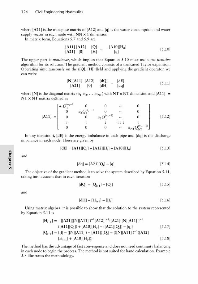
124 Civil Engineering Hydraulics
where [A21] is the transpose matrix of [A12] and [q] is the water consumption and watersupply vector in each node with NN × 1 dimension.
In matrix form, Equations 5.7 and 5.9 are[[A11] [A12][A21] [0]
] [[Q][H]
]=
[−[A10][H0]
[q]
][5.10]
The upper part is nonlinear, which implies that Equation 5.10 must use some iterativealgorithm for its solution. The gradient method consists of a truncated Taylor expansion.Operating simultaneously on the ([Q], [H]) field and applying the gradient operator, wecan write [
[N][A11]′ [A12][A21] [0]
] [[dQ][dH]
]=
[[dE][dq]
][5.11]
where [N] is the diagonal matrix (n1, n2, . . . , nNT) with NT × NT dimension and [A11]′ =NT × NT matrix defined as
[A11]′ =
⎡⎢⎢⎢⎢⎢⎣
𝛼1Q(n1−1)1 0 0 ⋯ 00 𝛼2Q(n2−1)
2 0 ⋯ 00 0 𝛼3Q(n3−1)
3 ⋯ 0⋮ ⋮ ⋮ ⋮ ⋮ ⋮ ⋮0 0 0 ⋯ 𝛼NTQ(nNT−1)
NT
⎤⎥⎥⎥⎥⎥⎦[5.12]
In any iteration i, [dE] is the energy imbalance in each pipe and [dq] is the dischargeimbalance in each node. These are given by
[dE] = [A11][Qi] + [A12][Hi] + [A10][H0] [5.13]
and
[dq] = [A21][Qi] − [q] [5.14]
The objective of the gradient method is to solve the system described by Equation 5.11,taking into account that in each iteration
[dQ] = [Qi+1] − [Qi] [5.15]
and
[dH] − [Hi+1] − [Hi] [5.16]
Using matrix algebra, it is possible to show that the solution to the system representedby Equation 5.11 is
[Hi+1] = −{[A21]([N][A11]′)−1[A12]}−1{[A21]([N][A11]′)−1
([A11][Qi]) + [A10][H0] − ([A21][Qi]) − [q]} [5.17]
[Qi+1] = {[I] − ([N][A11]′) − [A11]}[Qi] − {([N][A11]′)−1([A12]
[Hi+1] + [A10][H0])} [5.18]
The method has the advantage of fast convergence and does not need continuity balancingin each node to begin the process. The method is not suited for hand calculation. Example5.8 illustrates the methodology.
Ch
apter
5
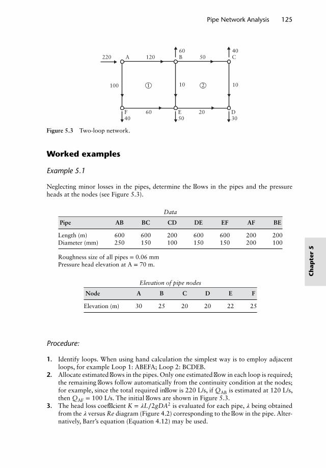
Pipe Network Analysis 125
100 1 2
A220 120 B C
D30
E 206050
F40
60
10
40
10
50
Figure 5.3 Two-loop network.
Worked examples
Example 5.1
Neglecting minor losses in the pipes, determine the flows in the pipes and the pressureheads at the nodes (see Figure 5.3).
Data
Pipe AB BC CD DE EF AF BE
Length (m) 600 600 200 600 600 200 200Diameter (mm) 250 150 100 150 150 200 100
Roughness size of all pipes = 0.06 mmPressure head elevation at A = 70 m.
Elevation of pipe nodes
Node A B C D E F
Elevation (m) 30 25 20 20 22 25
Procedure:
1. Identify loops. When using hand calculation the simplest way is to employ adjacentloops, for example Loop 1: ABEFA; Loop 2: BCDEB.
2. Allocate estimated flows in the pipes. Only one estimated flow in each loop is required;the remaining flows follow automatically from the continuity condition at the nodes;for example, since the total required inflow is 220 L/s, if QAB is estimated at 120 L/s,then QAF = 100 L/s. The initial flows are shown in Figure 5.3.
3. The head loss coefficient K = 𝜆L∕2gDA2 is evaluated for each pipe, 𝜆 being obtainedfrom the 𝜆 versus Re diagram (Figure 4.2) corresponding to the flow in the pipe. Alter-natively, Barr’s equation (Equation 4.12) may be used.
Ch
apte
r5
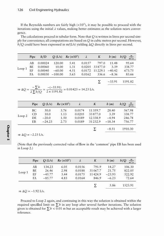
126 Civil Engineering Hydraulics
If the Reynolds numbers are fairly high (<| 105), it may be possible to proceed with theiterations using the initial 𝜆 values, making better estimates as the solution nears conver-gence.
The calculations proceed in tabular form. Note that Q is written in litres per second sim-ply for convenience; all computations are based on Q in cubic metres per second. However,h∕Q could have been expressed in m/(L/s) yielding ΔQ directly in litres per second.
Pipe k∕D Q (L/s) Re (×105) 𝝀 K h (m) h∕Q(
mm3∕s
)
AB 0.00024 120.00 5.41 0.0157 797.0 11.48 95.64BE 0.00060 10.00 1.31 0.0205 33 877.0 3.39 338.77Loop 1EF 0.00040 −60.00 4.51 0.0172 11 229.1 −40.42 673.75FA 0.00030 −100.00 5.63 0.0162 336.6 −8.36 83.66
∑−33.91 1191.82
⇒ ΔQ =−∑
h
2∑
h∕Q= −(−33.91)
2 × 1191.82= 0.01423 = 14.23 L/s.
Pipe Q (L/s) Re (×105) 𝝀 K h (m) h∕Q(
mm3∕s
)
BC 50.0 3.76 0.0174 11 359.7 28.40 567.98CD 10.0 1.13 0.0205 33 877.0 3.39 338.77Loop 2DE −20.0 1.50 0.0189 12 338.9 −4.94 246.78EB −24.23 2.73 0.0189 31 232.9 −18.34 756.77
∑−8.51 1910.30
⇒ ΔQ = −2.23 L/s.
(Note that the previously corrected value of flow in the ‘common’ pipe EB has been usedin Loop 2.)
Pipe Q (L/s) Re (×105) 𝝀 K h (m) h∕Q(
mm3∕s
)
AB 134.23 6.05 0.0156 791.9 14.27 106.30BE 26.46 2.98 0.0188 31 067.7 21.75 822.05Loop 1EF −45.77 3.44 0.0175 11 424.9 −23.93 522.92FA −85.77 4.83 0.0164 846.9 −6.23 72.64
∑5.86 1523.91
⇒ ΔQ = −1.92 L/s.
Proceed to Loop 2 again, and continuing in this way the solution is obtained within therequired specified limit on
∑h in any loop after several further iterations. The solution
given is obtained for∑
h < 0.01 m but an acceptable result may be achieved with a largertolerance.
Ch
apter
5
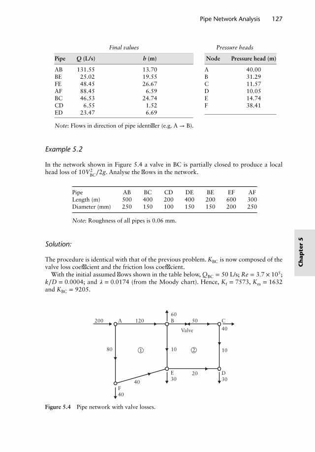
Pipe Network Analysis 127
Final values Pressure heads
Pipe Q (L/s) h (m) Node Pressure head (m)
AB 131.55 13.70 A 40.00BE 25.02 19.55 B 31.29FE 48.45 26.67 C 11.57AF 88.45 6.59 D 10.05BC 46.53 24.74 E 14.74CD 6.55 1.52 F 38.41ED 23.47 6.69
Note: Flows in direction of pipe identifier (e.g. A → B).
Example 5.2
In the network shown in Figure 5.4 a valve in BC is partially closed to produce a localhead loss of 10V2
BC∕2g. Analyse the flows in the network.
Pipe AB BC CD DE BE EF AFLength (m) 500 400 200 400 200 600 300Diameter (mm) 250 150 100 150 150 200 250
Note: Roughness of all pipes is 0.06 mm.
Solution:
The procedure is identical with that of the previous problem. KBC is now composed of thevalve loss coefficient and the friction loss coefficient.
With the initial assumed flows shown in the table below, QBC = 50 L/s; Re = 3.7 × 10⁵;k∕D = 0.0004; and 𝜆 = 0.0174 (from the Moody chart). Hence, Kf = 7573, Km = 1632and KBC = 9205.
200
Valve
A B60
1080 1 2
C
40
10
D30
E30
F40
40
120 50
20
Figure 5.4 Pipe network with valve losses.
Ch
apte
r5
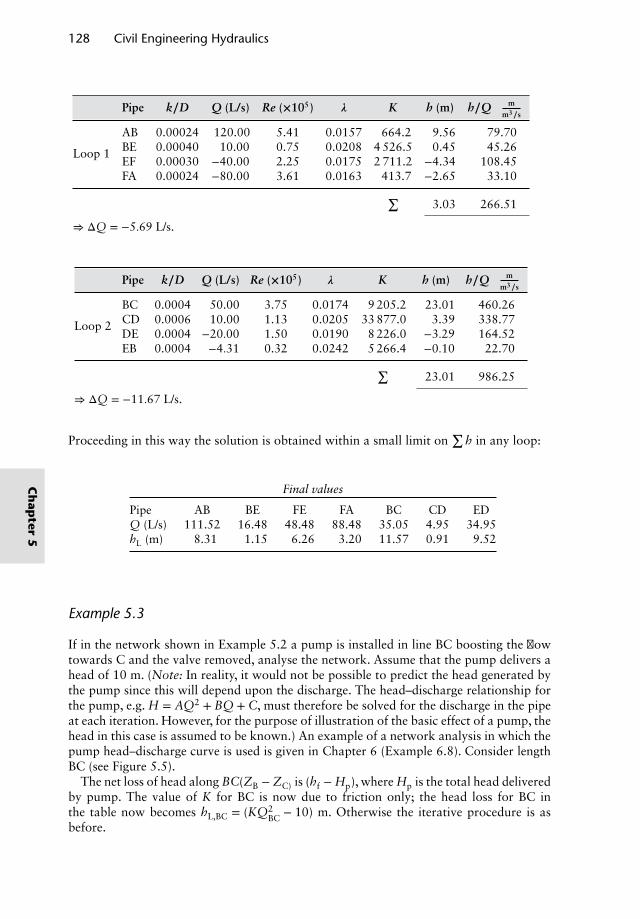
128 Civil Engineering Hydraulics
Pipe k∕D Q (L/s) Re (×105) 𝝀 K h (m) h∕Q(
mm3∕s
)
AB 0.00024 120.00 5.41 0.0157 664.2 9.56 79.70BE 0.00040 10.00 0.75 0.0208 4 526.5 0.45 45.26Loop 1EF 0.00030 −40.00 2.25 0.0175 2 711.2 −4.34 108.45FA 0.00024 −80.00 3.61 0.0163 413.7 −2.65 33.10
∑3.03 266.51
⇒ ΔQ = −5.69 L/s.
Pipe k∕D Q (L/s) Re (×105) 𝝀 K h (m) h∕Q(
mm3∕s
)
BC 0.0004 50.00 3.75 0.0174 9 205.2 23.01 460.26CD 0.0006 10.00 1.13 0.0205 33 877.0 3.39 338.77Loop 2DE 0.0004 −20.00 1.50 0.0190 8 226.0 −3.29 164.52EB 0.0004 −4.31 0.32 0.0242 5 266.4 −0.10 22.70
∑23.01 986.25
⇒ ΔQ = −11.67 L/s.
Proceeding in this way the solution is obtained within a small limit on∑
h in any loop:
Final values
Pipe AB BE FE FA BC CD EDQ (L/s) 111.52 16.48 48.48 88.48 35.05 4.95 34.95hL (m) 8.31 1.15 6.26 3.20 11.57 0.91 9.52
Example 5.3
If in the network shown in Example 5.2 a pump is installed in line BC boosting the flowtowards C and the valve removed, analyse the network. Assume that the pump delivers ahead of 10 m. (Note: In reality, it would not be possible to predict the head generated bythe pump since this will depend upon the discharge. The head–discharge relationship forthe pump, e.g. H = AQ2 + BQ + C, must therefore be solved for the discharge in the pipeat each iteration. However, for the purpose of illustration of the basic effect of a pump, thehead in this case is assumed to be known.) An example of a network analysis in which thepump head–discharge curve is used is given in Chapter 6 (Example 6.8). Consider lengthBC (see Figure 5.5).
The net loss of head along BC(ZB − ZC) is (hf − Hp), where Hp is the total head deliveredby pump. The value of K for BC is now due to friction only; the head loss for BC inthe table now becomes hL,BC = (KQ2
BC − 10) m. Otherwise the iterative procedure is asbefore.
Ch
apter
5
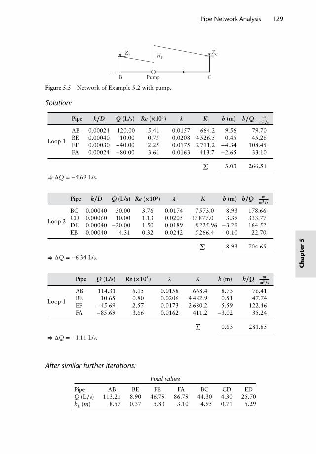
Pipe Network Analysis 129
CPumpB
HPZB ZC
Figure 5.5 Network of Example 5.2 with pump.
Solution:
Pipe k∕D Q (L/s) Re (×105) 𝝀 K h (m) h∕Q(
mm3∕s
)
AB 0.00024 120.00 5.41 0.0157 664.2 9.56 79.70BE 0.00040 10.00 0.75 0.0208 4 526.5 0.45 45.26Loop 1EF 0.00030 −40.00 2.25 0.0175 2 711.2 −4.34 108.45FA 0.00024 −80.00 3.61 0.0163 413.7 −2.65 33.10
∑3.03 266.51
⇒ ΔQ = −5.69 L/s.
Pipe k∕D Q (L/s) Re (×105) 𝝀 K h (m) h∕Q(
mm3∕s
)
BC 0.00040 50.00 3.76 0.0174 7 573.0 8.93 178.66CD 0.00060 10.00 1.13 0.0205 33 877.0 3.39 333.77Loop 2DE 0.00040 −20.00 1.50 0.0189 8 225.96 −3.29 164.52EB 0.00040 −4.31 0.32 0.0242 5 266.4 −0.10 22.70
∑8.93 704.65
⇒ ΔQ = −6.34 L/s.
Pipe Q (L/s) Re (×105) 𝝀 K h (m) h∕Q(
mm3∕s
)
AB 114.31 5.15 0.0158 668.4 8.73 76.41BE 10.65 0.80 0.0206 4 482.9 0.51 47.74Loop 1EF −45.69 2.57 0.0173 2 680.2 −5.59 122.46FA −85.69 3.66 0.0162 411.2 −3.02 35.24
∑0.63 281.85
⇒ ΔQ = −1.11 L/s.
After similar further iterations:
Final values
Pipe AB BE FE FA BC CD EDQ (L∕s) 113.21 8.90 46.79 86.79 44.30 4.30 25.70hL (m) 8.57 0.37 5.83 3.10 4.95 0.71 5.29
Ch
apte
r5
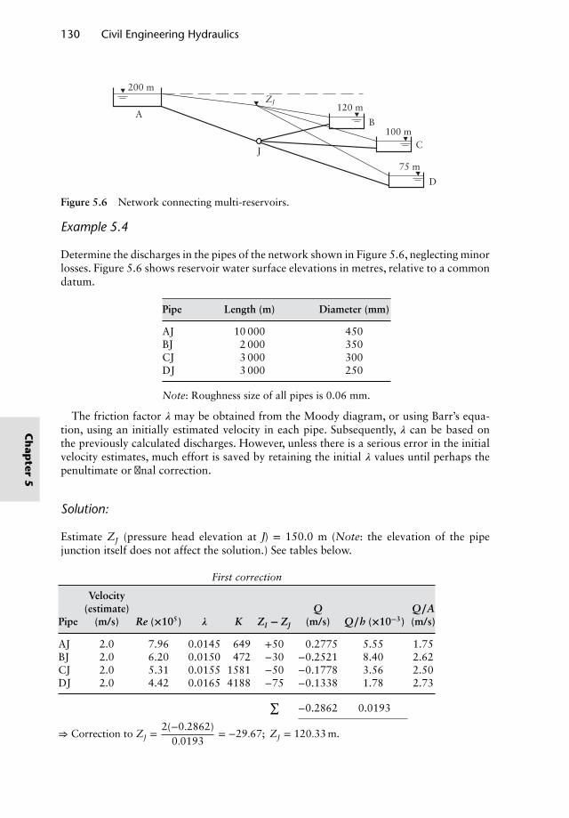
130 Civil Engineering Hydraulics
C
D
B
J
A
75 m
100 m
120 m
200 mZJ
Figure 5.6 Network connecting multi-reservoirs.
Example 5.4
Determine the discharges in the pipes of the network shown in Figure 5.6, neglecting minorlosses. Figure 5.6 shows reservoir water surface elevations in metres, relative to a commondatum.
Pipe Length (m) Diameter (mm)
AJ 10 000 450BJ 2 000 350CJ 3 000 300DJ 3 000 250
Note: Roughness size of all pipes is 0.06 mm.
The friction factor 𝜆 may be obtained from the Moody diagram, or using Barr’s equa-tion, using an initially estimated velocity in each pipe. Subsequently, 𝜆 can be based onthe previously calculated discharges. However, unless there is a serious error in the initialvelocity estimates, much effort is saved by retaining the initial 𝜆 values until perhaps thepenultimate or final correction.
Solution:
Estimate ZJ (pressure head elevation at J) = 150.0 m (Note: the elevation of the pipejunction itself does not affect the solution.) See tables below.
First correction
Velocity(estimate) Q Q∕A
Pipe (m/s) Re (×105) 𝝀 K ZI − ZJ (m/s) Q∕h (×10−3) (m/s)
AJ 2.0 7.96 0.0145 649 +50 0.2775 5.55 1.75BJ 2.0 6.20 0.0150 472 −30 −0.2521 8.40 2.62CJ 2.0 5.31 0.0155 1581 −50 −0.1778 3.56 2.50DJ 2.0 4.42 0.0165 4188 −75 −0.1338 1.78 2.73
∑−0.2862 0.0193
⇒ Correction to ZJ =2(−0.2862)
0.0193= −29.67; ZJ = 120.33 m.
Ch
apter
5
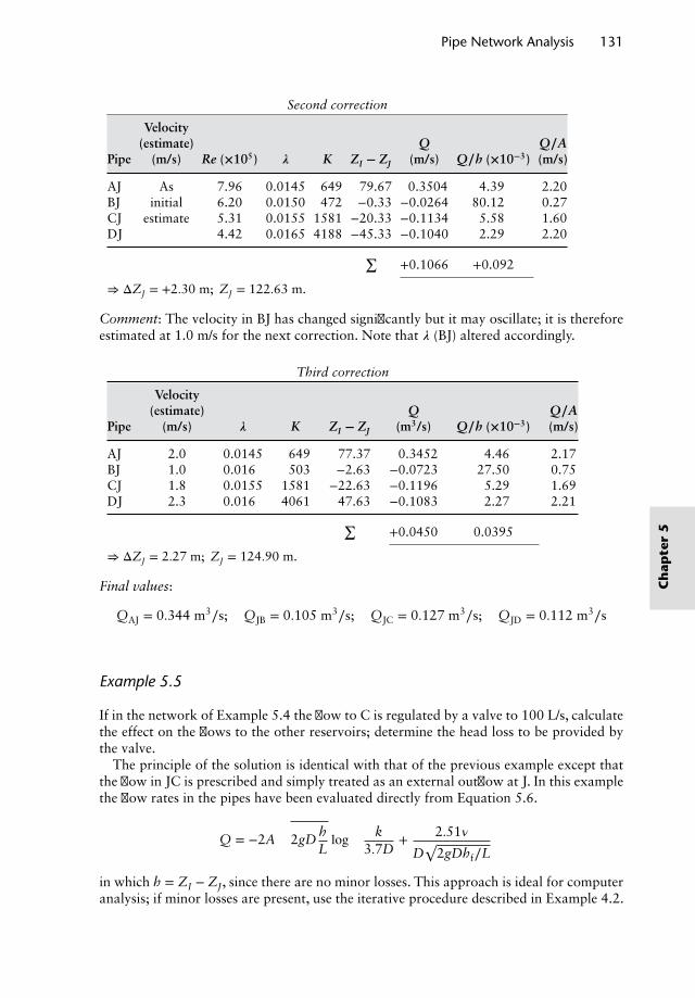
Pipe Network Analysis 131
Second correction
Velocity(estimate) Q Q∕A
Pipe (m/s) Re (×105) 𝝀 K ZI − ZJ (m/s) Q∕h (×10−3) (m/s)
AJ As 7.96 0.0145 649 79.67 0.3504 4.39 2.20BJ initial 6.20 0.0150 472 −0.33 −0.0264 80.12 0.27CJ estimate 5.31 0.0155 1581 −20.33 −0.1134 5.58 1.60DJ 4.42 0.0165 4188 −45.33 −0.1040 2.29 2.20
∑+0.1066 +0.092
⇒ ΔZJ = +2.30 m; ZJ = 122.63 m.
Comment: The velocity in BJ has changed significantly but it may oscillate; it is thereforeestimated at 1.0 m/s for the next correction. Note that 𝜆 (BJ) altered accordingly.
Third correction
Velocity(estimate) Q Q∕A
Pipe (m/s) 𝝀 K ZI − ZJ (m3/s) Q∕h (×10−3) (m/s)
AJ 2.0 0.0145 649 77.37 0.3452 4.46 2.17BJ 1.0 0.016 503 −2.63 −0.0723 27.50 0.75CJ 1.8 0.0155 1581 −22.63 −0.1196 5.29 1.69DJ 2.3 0.016 4061 47.63 −0.1083 2.27 2.21
∑+0.0450 0.0395
⇒ ΔZJ = 2.27 m; ZJ = 124.90 m.
Final values:
QAJ = 0.344 m3∕s; QJB = 0.105 m3∕s; QJC = 0.127 m3∕s; QJD = 0.112 m3∕s
Example 5.5
If in the network of Example 5.4 the flow to C is regulated by a valve to 100 L/s, calculatethe effect on the flows to the other reservoirs; determine the head loss to be provided bythe valve.
The principle of the solution is identical with that of the previous example except thatthe flow in JC is prescribed and simply treated as an external outflow at J. In this examplethe flow rates in the pipes have been evaluated directly from Equation 5.6.
Q = −2A
√2gD
hLlog
(k
3.7D+ 2.51𝜈
D√
2gDhf∕L
)
in which h = ZI − ZJ, since there are no minor losses. This approach is ideal for computeranalysis; if minor losses are present, use the iterative procedure described in Example 4.2.
Ch
apte
r5
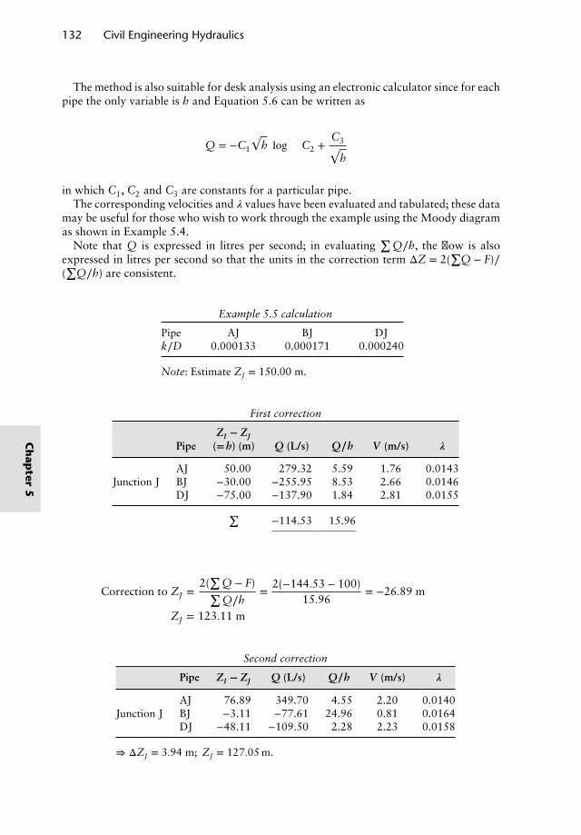
132 Civil Engineering Hydraulics
The method is also suitable for desk analysis using an electronic calculator since for eachpipe the only variable is h and Equation 5.6 can be written as
Q = −C1
√h log
(C2 +
C3√h
)
in which C1, C2 and C3 are constants for a particular pipe.The corresponding velocities and 𝜆 values have been evaluated and tabulated; these data
may be useful for those who wish to work through the example using the Moody diagramas shown in Example 5.4.
Note that Q is expressed in litres per second; in evaluating∑
Q∕h, the flow is alsoexpressed in litres per second so that the units in the correction term ΔZ = 2(
∑Q − F)∕
(∑
Q∕h) are consistent.
Example 5.5 calculation
Pipe AJ BJ DJk∕D 0.000133 0.000171 0.000240
Note: Estimate ZJ = 150.00 m.
First correction
ZI − ZJ
Pipe (=h) (m) Q (L/s) Q∕h V (m/s) 𝝀
AJ 50.00 279.32 5.59 1.76 0.0143Junction J BJ −30.00 −255.95 8.53 2.66 0.0146
DJ −75.00 −137.90 1.84 2.81 0.0155
∑−114.53 15.96
Correction to ZJ =2(∑
Q − F)∑Q∕h
=2(−144.53 − 100)
15.96= −26.89 m
ZJ = 123.11 m
Second correction
Pipe ZI − ZJ Q (L/s) Q∕h V (m/s) 𝝀
AJ 76.89 349.70 4.55 2.20 0.0140Junction J BJ −3.11 −77.61 24.96 0.81 0.0164
DJ −48.11 −109.50 2.28 2.23 0.0158
⇒ ΔZJ = 3.94 m; ZJ = 127.05 m.
Ch
apter
5
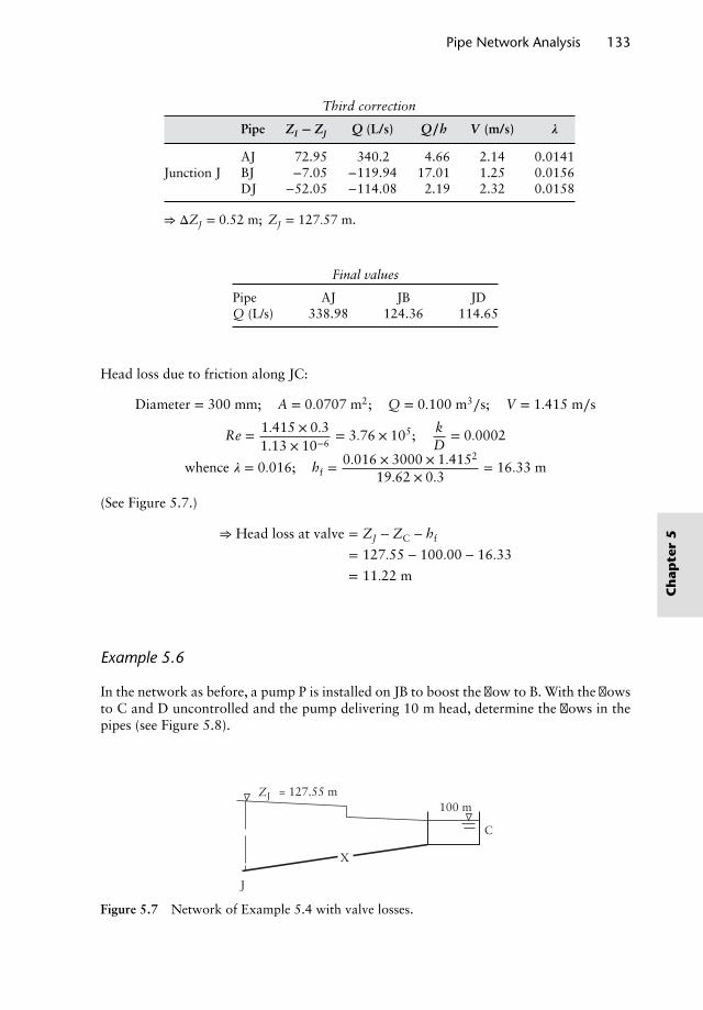
Pipe Network Analysis 133
Third correction
Pipe ZI − ZJ Q (L/s) Q∕h V (m/s) 𝝀
AJ 72.95 340.2 4.66 2.14 0.0141Junction J BJ −7.05 −119.94 17.01 1.25 0.0156
DJ −52.05 −114.08 2.19 2.32 0.0158
⇒ ΔZJ = 0.52 m; ZJ = 127.57 m.
Final values
Pipe AJ JB JDQ (L/s) 338.98 124.36 114.65
Head loss due to friction along JC:
Diameter = 300 mm; A = 0.0707 m2; Q = 0.100 m3∕s; V = 1.415 m∕s
Re = 1.415 × 0.31.13 × 10−6
= 3.76 × 10⁵; kD
= 0.0002
whence 𝜆 = 0.016; hf =0.016 × 3000 × 1.4152
19.62 × 0.3= 16.33 m
(See Figure 5.7.)
⇒ Head loss at valve = ZJ − ZC − hf
= 127.55 − 100.00 − 16.33
= 11.22 m
Example 5.6
In the network as before, a pump P is installed on JB to boost the flow to B. With the flowsto C and D uncontrolled and the pump delivering 10 m head, determine the flows in thepipes (see Figure 5.8).
C
X
J
ZJ = 127.55 m100 m
Figure 5.7 Network of Example 5.4 with valve losses.
Ch
apte
r5
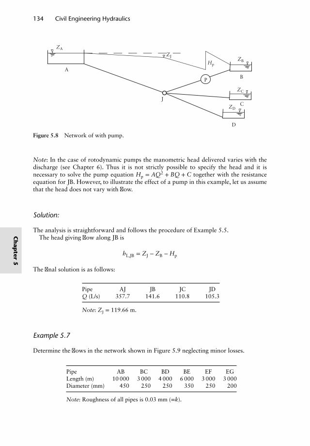
134 Civil Engineering Hydraulics
J
ZJ
ZA
ZB
ZC
ZD
Hp
BP
C
D
A
Figure 5.8 Network of with pump.
Note: In the case of rotodynamic pumps the manometric head delivered varies with thedischarge (see Chapter 6). Thus it is not strictly possible to specify the head and it isnecessary to solve the pump equation Hp = AQ2 + BQ + C together with the resistanceequation for JB. However, to illustrate the effect of a pump in this example, let us assumethat the head does not vary with flow.
Solution:
The analysis is straightforward and follows the procedure of Example 5.5.The head giving flow along JB is
hL,JB = ZJ − ZB − Hp
The final solution is as follows:
Pipe AJ JB JC JDQ (L/s) 357.7 141.6 110.8 105.3
Note: ZJ = 119.66 m.
Example 5.7
Determine the flows in the network shown in Figure 5.9 neglecting minor losses.
Pipe AB BC BD BE EF EGLength (m) 10 000 3 000 4 000 6 000 3 000 3 000Diameter (mm) 450 250 250 350 250 200
Note: Roughness of all pipes is 0.03 mm (=k).
Ch
apter
5
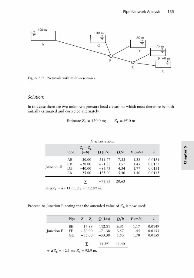
Pipe Network Analysis 135
60 m
75 m
80 m100 m
150 m
A C
D
B
EG
F
Figure 5.9 Network with multi-reservoirs.
Solution:
In this case there are two unknown pressure head elevations which must therefore be bothinitially estimated and corrected alternately.
Estimate ZB = 120.0 m; ZE = 95.0 m
First correction
ZI − ZJ
Pipe (=h) Q (L/s) Q∕h V (m/s) 𝝀
AB 30.00 219.77 7.33 1.38 0.0139
Junction BCB −20.00 −71.38 3.57 1.45 0.0155DB −40.00 −86.75 4.34 1.77 0.0151EB −25.00 −135.00 5.40 1.40 0.0145
∑−73.35 20.63
⇒ ΔZB = +7.11 m; ZB = 112.89 m.
Proceed to Junction E noting that the amended value of ZB is now used:
Pipe ZI − ZJ Q (L/s) Q∕h V (m/s) 𝝀
BE 17.89 112.81 6.31 1.17 0.0149Junction E FE −20.00 −71.38 3.57 1.45 0.0155
GE −35.00 −53.38 1.53 1.70 0.0159
∑11.95 11.40
⇒ ΔZE = −2.1 m; ZE = 92.9 m.
Ch
apte
r5
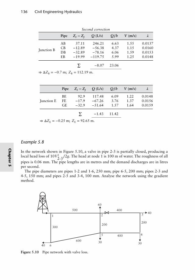
136 Civil Engineering Hydraulics
Second correction
Pipe ZI − ZJ Q (L/s) Q∕h V (m/s) 𝝀
AB 37.11 246.21 6.63 1.55 0.0137
Junction B CB −12.89 −56.38 4.37 1.15 0.0160DB −32.89 −78.16 6.06 1.59 0.0153EB −19.99 −119.75 5.99 1.25 0.0148
∑−8.07 23.06
⇒ ΔZB = −0.7 m; ZB = 112.19 m.
Pipe ZI − ZJ Q (L/s) Q∕h V (m/s) 𝝀
BE 92.9 117.48 6.09 1.22 0.0148Junction E FE −17.9 −67.26 3.76 1.37 0.0156
GE −32.9 −51.64 1.57 1.64 0.0159
∑−1.43 11.42
⇒ ΔZE = −0.25 m; ZE = 92.65 m.
Example 5.8
In the network shown in Figure 5.10, a valve in pipe 2-3 is partially closed, producing alocal head loss of 10V2
2-3∕2g. The head at node 1 is 100 m of water. The roughness of all
pipes is 0.06 mm. The pipe lengths are in metres and the demand discharges are in litresper second.
The pipe diameters are pipes 1-2 and 1-6, 250 mm; pipe 6-5, 200 mm; pipes 2-3 and4-5, 150 mm; and pipes 2-5 and 3-4, 100 mm. Analyse the network using the gradientmethod.
60
500
60040 6
300
1 2
400
200200
40
30
4
3
5
30
400
Figure 5.10 Pipe network with valve loss.
Ch
apter
5
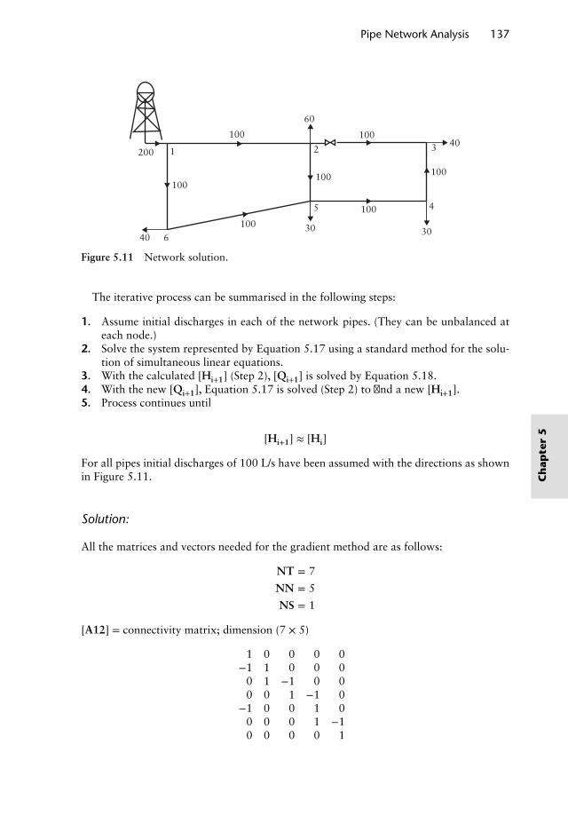
Pipe Network Analysis 137
60
100
10040 6
100
1200 2
100
100 100
40
30
4
3
5
30
100
Figure 5.11 Network solution.
The iterative process can be summarised in the following steps:
1. Assume initial discharges in each of the network pipes. (They can be unbalanced ateach node.)
2. Solve the system represented by Equation 5.17 using a standard method for the solu-tion of simultaneous linear equations.
3. With the calculated [Hi+1] (Step 2), [Qi+1] is solved by Equation 5.18.4. With the new [Qi+1], Equation 5.17 is solved (Step 2) to find a new [Hi+1].5. Process continues until
[Hi+1] ≈ [Hi]
For all pipes initial discharges of 100 L/s have been assumed with the directions as shownin Figure 5.11.
Solution:
All the matrices and vectors needed for the gradient method are as follows:
NT = 7
NN = 5
NS = 1
[A12] = connectivity matrix; dimension (7 × 5)
|||||||||||||||
1 0 0 0 0−1 1 0 0 0
0 1 −1 0 00 0 1 −1 0
−1 0 0 1 00 0 0 1 −10 0 0 0 1
|||||||||||||||
Ch
apte
r5
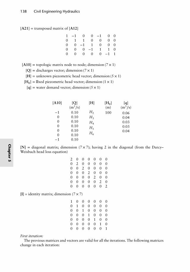
138 Civil Engineering Hydraulics
[A21] = transposed matrix of [A12]
|||||||||||
1 −1 0 0 −1 0 00 1 1 0 0 0 00 0 −1 1 0 0 00 0 0 −1 1 1 00 0 0 0 0 −1 1
|||||||||||[A10] = topologic matrix node to node; dimension (7 × 1)
[Q] = discharges vector; dimension (7 × 1)
[H] = unknown piezometric head vector; dimension (5 × 1)
[H0] = fixed piezometric head vector; dimension (1 × 1)
[q] = water demand vector; dimension (5 × 1)
[A10] [Q] [H] [H0] [q](m3∕s) (m) (m3∕s)|||||||||||||||
−100000
−1
|||||||||||||||
|||||||||||||||
0.100.100.100.100.100.100.10
|||||||||||||||
||||||||||||
H2
H3
H4
H5
H6
||||||||||||
||100 || |||||||||||
0.060.040.030.030.04
|||||||||||
[N] = diagonal matrix; dimension (7 × 7); having 2 in the diagonal (from the Darcy–Weisbach head loss equation)
|||||||||||||||
2 0 0 0 0 0 00 2 0 0 0 0 00 0 2 0 0 0 00 0 0 2 0 0 00 0 0 0 2 0 00 0 0 0 0 2 00 0 0 0 0 0 2
|||||||||||||||[I] = identity matrix; dimension (7 × 7)
|||||||||||||||
1 0 0 0 0 0 00 1 0 0 0 0 00 0 1 0 0 0 00 0 0 1 0 0 00 0 0 0 1 0 00 0 0 0 0 1 00 0 0 0 0 0 1
|||||||||||||||First iteration:
The previous matrices and vectors are valid for all the iterations. The following matriceschange in each iteration:
Ch
apter
5
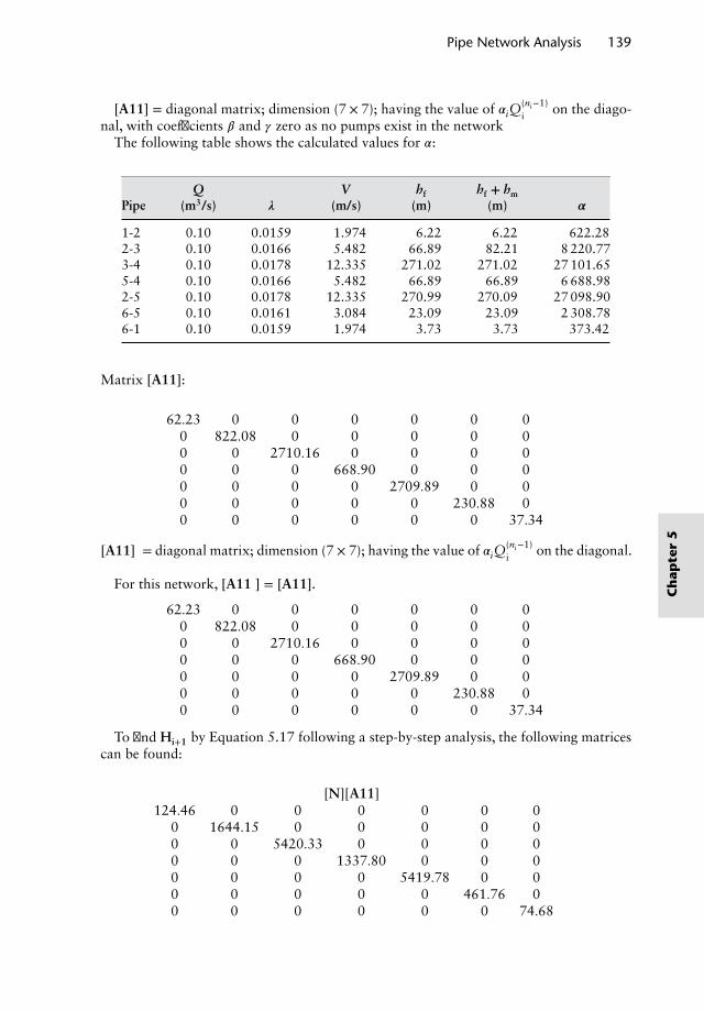
Pipe Network Analysis 139
[A11] = diagonal matrix; dimension (7 × 7); having the value of 𝛼iQ(ni−1)i on the diago-
nal, with coefficients 𝛽 and 𝛾 zero as no pumps exist in the networkThe following table shows the calculated values for 𝛼:
Q V hf hf + hmPipe (m3/s) 𝝀 (m/s) (m) (m) 𝜶
1-2 0.10 0.0159 1.974 6.22 6.22 622.282-3 0.10 0.0166 5.482 66.89 82.21 8 220.773-4 0.10 0.0178 12.335 271.02 271.02 27 101.655-4 0.10 0.0166 5.482 66.89 66.89 6 688.982-5 0.10 0.0178 12.335 270.99 270.09 27 098.906-5 0.10 0.0161 3.084 23.09 23.09 2 308.786-1 0.10 0.0159 1.974 3.73 3.73 373.42
Matrix [A11]:
|||||||||||||||
62.23 0 0 0 0 0 00 822.08 0 0 0 0 00 0 2710.16 0 0 0 00 0 0 668.90 0 0 00 0 0 0 2709.89 0 00 0 0 0 0 230.88 00 0 0 0 0 0 37.34
|||||||||||||||[A11]′ = diagonal matrix; dimension (7 × 7); having the value of 𝛼iQ
(ni−1)i on the diagonal.
For this network, [A11′] = [A11].
|||||||||||||||
62.23 0 0 0 0 0 00 822.08 0 0 0 0 00 0 2710.16 0 0 0 00 0 0 668.90 0 0 00 0 0 0 2709.89 0 00 0 0 0 0 230.88 00 0 0 0 0 0 37.34
|||||||||||||||To find Hi+1 by Equation 5.17 following a step-by-step analysis, the following matrices
can be found:
[N][A11]′|||||||||||||||
124.46 0 0 0 0 0 00 1644.15 0 0 0 0 00 0 5420.33 0 0 0 00 0 0 1337.80 0 0 00 0 0 0 5419.78 0 00 0 0 0 0 461.76 00 0 0 0 0 0 74.68
|||||||||||||||
Ch
apte
r5
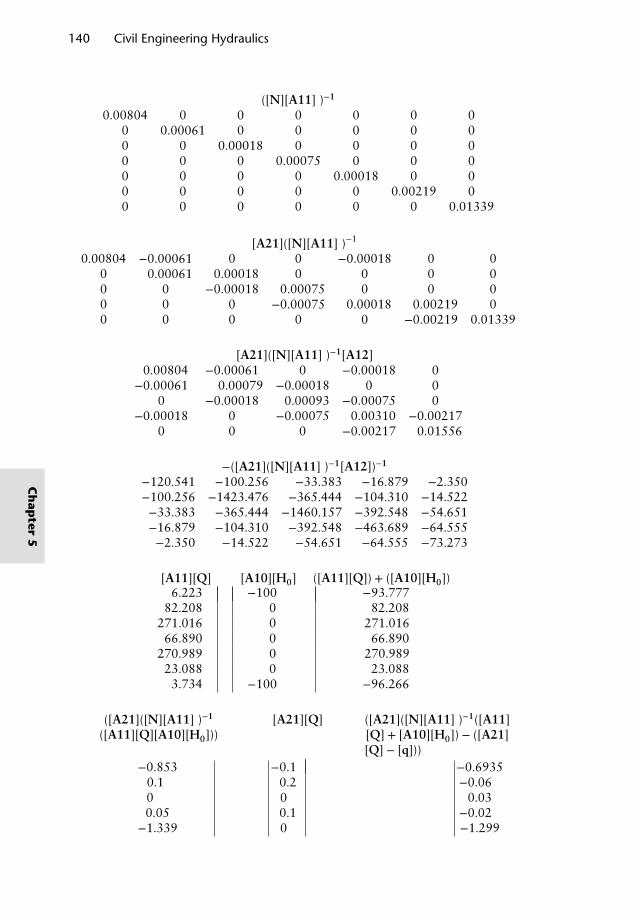
140 Civil Engineering Hydraulics
([N][A11]′)−1|||||||||||||||
0.00804 0 0 0 0 0 00 0.00061 0 0 0 0 00 0 0.00018 0 0 0 00 0 0 0.00075 0 0 00 0 0 0 0.00018 0 00 0 0 0 0 0.00219 00 0 0 0 0 0 0.01339
|||||||||||||||[A21]([N][A11]′)−1|||||||||||
0.00804 −0.00061 0 0 −0.00018 0 00 0.00061 0.00018 0 0 0 00 0 −0.00018 0.00075 0 0 00 0 0 −0.00075 0.00018 0.00219 00 0 0 0 0 −0.00219 0.01339
|||||||||||[A21]([N][A11]′)−1[A12]|||||||||||
0.00804 −0.00061 0 −0.00018 0−0.00061 0.00079 −0.00018 0 0
0 −0.00018 0.00093 −0.00075 0−0.00018 0 −0.00075 0.00310 −0.00217
0 0 0 −0.00217 0.01556
|||||||||||−([A21]([N][A11]′)−1[A12])−1|||||||||||
−120.541 −100.256 −33.383 −16.879 −2.350−100.256 −1423.476 −365.444 −104.310 −14.522−33.383 −365.444 −1460.157 −392.548 −54.651−16.879 −104.310 −392.548 −463.689 −64.555−2.350 −14.522 −54.651 −64.555 −73.273
|||||||||||[A11][Q] [A10][H0] ([A11][Q]) + ([A10][H0])|||||||||||||||
6.223 −100 −93.77782.208 0 82.208
271.016 0 271.01666.890 0 66.890
270.989 0 270.98923.088 0 23.0883.734 −100 −96.266
|||||||||||||||([A21]([N][A11]′)−1 [A21][Q] ([A21]([N][A11]′)−1([A11]
([A11][Q][A10][H0])) [Q] + [A10][H0]) − ([A21][Q] − [q]))|||||||||||
−0.853 −0.1 −0.69350.1 0.2 −0.060 0 0.030.05 0.1 −0.02
−1.339 0 −1.299
|||||||||||
Ch
apter
5
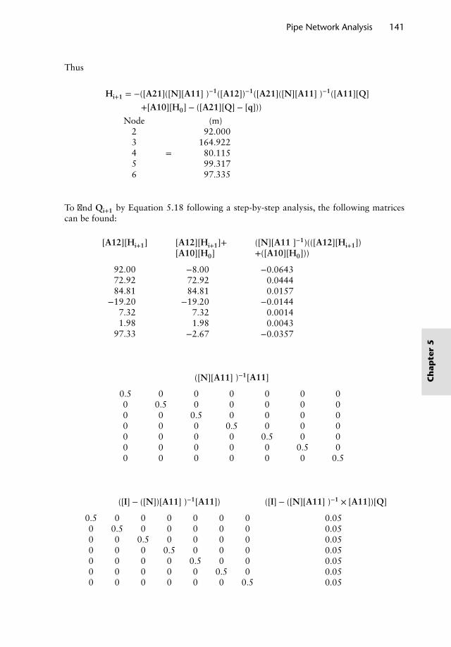
Pipe Network Analysis 141
Thus
Hi+1 = −([A21]([N][A11]′)−1([A12])−1([A21]([N][A11]′)−1([A11][Q]
+[A10][H0] − ([A21][Q] − [q]))
Node (m)|||||||||||
23456
|||||||||||=
|||||||||||
92.000164.92280.11599.31797.335
|||||||||||To find Qi+1 by Equation 5.18 following a step-by-step analysis, the following matricescan be found:
[A12][Hi+1] [A12][Hi+1]+ ([N][A11′]−1)(([A12][Hi+1])[A10][H0] +([A10][H0]))
|||||||||||||||
92.0072.9284.81
−19.207.321.98
97.33
|||||||||||||||
|||||||||||||||
−8.0072.9284.81
−19.207.321.98
−2.67
|||||||||||||||
|||||||||||||||
−0.06430.04440.0157
−0.01440.00140.0043
−0.0357
|||||||||||||||
([N][A11]′)−1[A11]
|||||||||||||||
0.5 0 0 0 0 0 00 0.5 0 0 0 0 00 0 0.5 0 0 0 00 0 0 0.5 0 0 00 0 0 0 0.5 0 00 0 0 0 0 0.5 00 0 0 0 0 0 0.5
|||||||||||||||
([I] − ([N])[A11]′)−1[A11]) ([I] − ([N][A11]′)−1 × [A11])[Q]
|||||||||||||||
0.5 0 0 0 0 0 00 0.5 0 0 0 0 00 0 0.5 0 0 0 00 0 0 0.5 0 0 00 0 0 0 0.5 0 00 0 0 0 0 0.5 00 0 0 0 0 0 0.5
|||||||||||||||
|||||||||||||||
0.050.050.050.050.050.050.05
|||||||||||||||
Ch
apte
r5
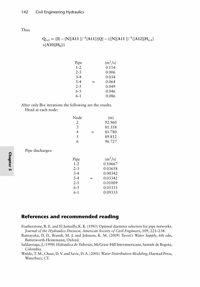
142 Civil Engineering Hydraulics
Thus
Qi+1 = ([I] − [N][A11′])−1[A11])[Q] − (([N][A11′])−1([A12][Hi+1]
+[A10][H0]))
Pipe (m3∕s)|||||||||||||||
1-22-33-45-42-56-56-1
|||||||||||||||
=
|||||||||||||||
0.1140.0060.0340.0640.0490.0460.086
|||||||||||||||After only five iterations the following are the results.
Head at each node:
Node (m)|||||||||||
23456
|||||||||||=
|||||||||||
92.96081.35881.78089.81296.727
|||||||||||Pipe discharges:
Pipe (m3∕s)|||||||||||||||
1-22-33-45-42-56-56-1
|||||||||||||||
=
|||||||||||||||
0.106670.036580.003420.033420.010090.053330.09333
|||||||||||||||
References and recommended reading
Featherstone, R. E. and El Jumailly, K. K. (1983) Optimal diameter selection for pipe networks.Journal of the Hydraulics Division, American Society of Civil Engineers, 109, 221–234.
Ratnayaka, D. D., Brandt, M. J. and Johnson, K. M. (2009) Twort’s Water Supply, 6th edn,Butterworth-Heinemann, Oxford.
Saldarriaga, J. (1998) Hidraulica de Tuberias, McGraw-Hill Interamericana, Santafe de Bogota,Colombia.
Walski, T. M., Chase, D. V. and Savic, D. A. (2001) Water Distribution Modeling, Haestad Press,Waterbury, CT.
Ch
apter
5
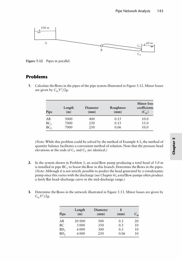
Pipe Network Analysis 143
60 mC1
C2
B
A
100 m
Figure 5.12 Pipes in parallel.
Problems
1. Calculate the flows in the pipes of the pipe system illustrated in Figure 5.12. Minor lossesare given by CmV2∕2g.
Minor lossLength Diameter Roughness coefficients
Pipe (m) (mm) (mm) (Cm)
AB 5000 400 0.15 10.0BC1 7000 250 0.15 15.0BC2 7000 250 0.06 10.0
(Note: While this problem could be solved by the method of Example 4.1, the method ofquantity balance facilitates a convenient method of solution. Note that the pressure headelevations at the ends of C1 and C2 are identical.)
2. In the system shown in Problem 1, an axial flow pump producing a total head of 5.0 mis installed in pipe BC1 to boost the flow in this branch. Determine the flows in the pipes.(Note: Although it is not strictly possible to predict the head generated by a rotodynamicpump since this varies with the discharge (see Chapter 6), axial flow pumps often producea fairly flat head–discharge curve in the mid-discharge range.)
3. Determine the flows in the network illustrated in Figure 5.13. Minor losses are given byCmV2∕2g.
Length Diameter kPipe (m) (mm) (mm) Cm
AB 20 000 500 0.3 20BC 5 000 350 0.3 10BD1 6 000 300 0.3 10BD2 6 000 250 0.06 10
Ch
apte
r5
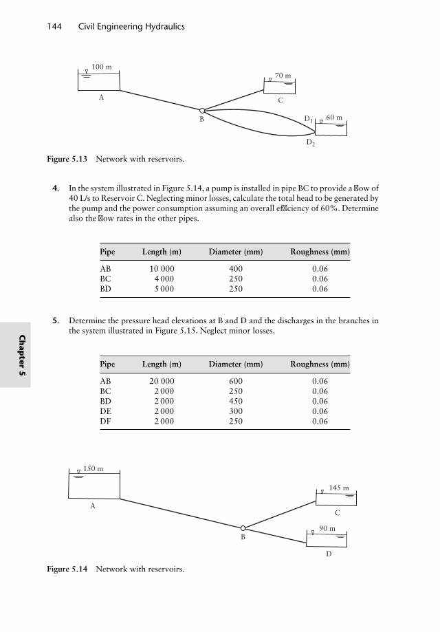
144 Civil Engineering Hydraulics
60 m
70 m100 m
A
D1
D2
C
B
Figure 5.13 Network with reservoirs.
4. In the system illustrated in Figure 5.14, a pump is installed in pipe BC to provide a flow of40 L/s to Reservoir C. Neglecting minor losses, calculate the total head to be generated bythe pump and the power consumption assuming an overall efficiency of 60%. Determinealso the flow rates in the other pipes.
Pipe Length (m) Diameter (mm) Roughness (mm)
AB 10 000 400 0.06BC 4 000 250 0.06BD 5 000 250 0.06
5. Determine the pressure head elevations at B and D and the discharges in the branches inthe system illustrated in Figure 5.15. Neglect minor losses.
Pipe Length (m) Diameter (mm) Roughness (mm)
AB 20 000 600 0.06BC 2 000 250 0.06BD 2 000 450 0.06DE 2 000 300 0.06DF 2 000 250 0.06
90 m
145 m
A
150 m
C
D
B
Figure 5.14 Network with reservoirs.
Ch
apter
5
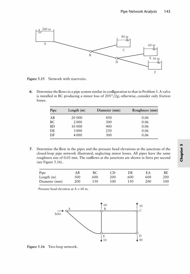
Pipe Network Analysis 145
60 m
80 m
200 m
C
D
B
A
50 m
F
E
Figure 5.15 Network with reservoirs.
6. Determine the flows in a pipe system similar in configuration to that in Problem 5. A valveis installed in BC producing a minor loss of 20V2∕2g; otherwise, consider only frictionlosses.
Pipe Length (m) Diameter (mm) Roughness (mm)
AB 20 000 450 0.06BC 2 000 300 0.06BD 10 000 400 0.06DE 3 000 250 0.06DF 4 000 300 0.06
7. Determine the flow in the pipes and the pressure head elevations at the junctions of theclosed-loop pipe network illustrated, neglecting minor losses. All pipes have the sameroughness size of 0.03 mm. The outflows at the junctions are shown in litres per second(see Figure 5.16).
Pipe AB BC CD DE EA BELength (m) 500 600 200 600 600 200Diameter (mm) 200 150 100 150 200 100
Pressure head elevation at A = 60 m.
50C
60BA
Inlet
40D
50E
Figure 5.16 Two-loop network.
Ch
apte
r5
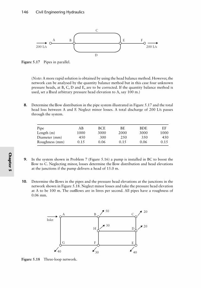
146 Civil Engineering Hydraulics
EB
200 L/s200 L/s
F
D
A
C
Figure 5.17 Pipes in parallel.
(Note: A more rapid solution is obtained by using the head balance method. However, thenetwork can be analysed by the quantity balance method but in this case four unknownpressure heads, at B, C, D and E, are to be corrected. If the quantity balance method isused, set a fixed arbitrary pressure head elevation to A, say 100 m.)
8. Determine the flow distribution in the pipe system illustrated in Figure 5.17 and the totalhead loss between A and F. Neglect minor losses. A total discharge of 200 L/s passesthrough the system.
Pipe AB BCE BE BDE EFLength (m) 1000 3000 2000 3000 1000Diameter (mm) 450 300 250 350 450Roughness (mm) 0.15 0.06 0.15 0.06 0.15
9. In the system shown in Problem 7 (Figure 5.16) a pump is installed in BC to boost theflow to C. Neglecting minor, losses determine the flow distribution and head elevationsat the junctions if the pump delivers a head of 15.0 m.
10. Determine the flows in the pipes and the pressure head elevations at the junctions in thenetwork shown in Figure 5.18. Neglect minor losses and take the pressure head elevationat A to be 100 m. The outflows are in litres per second. All pipes have a roughness of0.06 mm.
CBA50
H
FG E
D
20
20
4030
30
Inlet
40
Figure 5.18 Three-loop network.
Ch
apter
5
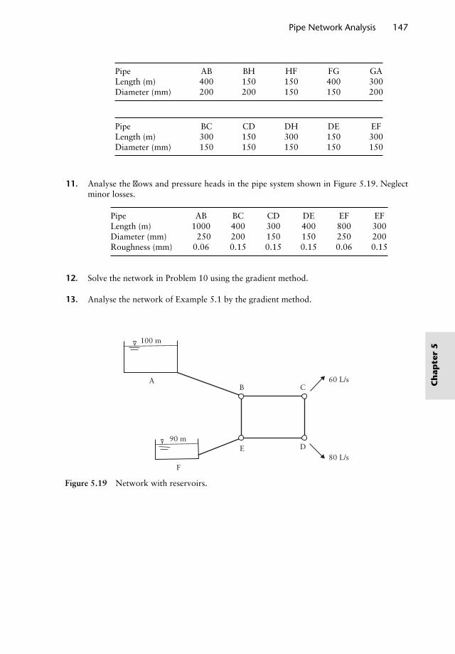
Pipe Network Analysis 147
Pipe AB BH HF FG GALength (m) 400 150 150 400 300Diameter (mm) 200 200 150 150 200
Pipe BC CD DH DE EFLength (m) 300 150 300 150 300Diameter (mm) 150 150 150 150 150
11. Analyse the flows and pressure heads in the pipe system shown in Figure 5.19. Neglectminor losses.
Pipe AB BC CD DE EF EFLength (m) 1000 400 300 400 800 300Diameter (mm) 250 200 150 150 250 200Roughness (mm) 0.06 0.15 0.15 0.15 0.06 0.15
12. Solve the network in Problem 10 using the gradient method.
13. Analyse the network of Example 5.1 by the gradient method.
90 m
AB C
60 L/s
80 L/sD
F
E
100 m
Figure 5.19 Network with reservoirs.
Ch
apte
r5

Chapter 6Pump–Pipeline SystemAnalysis and Design
6.1 Introduction
This chapter deals with the analysis and design of pipe systems which incorporate rotody-namic pumps. The civil engineer is mostly concerned with pump selection in the design ofpumping stations and therefore the design of the shape of pump impellers will not be dealtwith here. Rotodynamic pumps can be subclassified into three main categories accordingto the shape of the impellers:(i) Centrifugal (radial flow)(ii) Mixed flow(iii) Propeller (axial flow)For the same power input and efficiency the centrifugal type would generate a relativelylarge pressure head with a low discharge, while the propeller type a relatively large dis-charge at a low head with the mixed flow having characteristics somewhere between theother two.
Pump types may be more explicitly defined by the parameter called specific speed (N s),expressed by
N s =N√
Q
H3∕4
where Q is the discharge, H the total head and N the rotational speed (rev/min). Thisexpression is derived from dynamical similarity considerations and may be interpreted asthe speed in revolutions per minute at which a geometrically scaled model would have tooperate to deliver unit discharge (e.g. 1 L/s) when generating unit head (e.g. 1 m).
Pump type N s range (Q, L/s; H, m)
Centrifugal Up to 2400Mixed flow 2400 to 5000Axial flow Above 3400
Nalluri & Featherstone’s Civil Engineering Hydraulics: Essential Theory with Worked Examples,Sixth Edition. Martin Marriott.© 2016 John Wiley & Sons, Ltd. Published 2016 by John Wiley & Sons, Ltd.Companion Website: www.wiley.com/go/Marriott
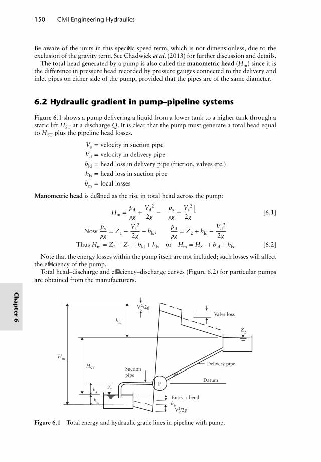
150 Civil Engineering Hydraulics
Be aware of the units in this specific speed term, which is not dimensionless, due to theexclusion of the gravity term. See Chadwick et al. (2013) for further discussion and details.
The total head generated by a pump is also called the manometric head (Hm) since it isthe difference in pressure head recorded by pressure gauges connected to the delivery andinlet pipes on either side of the pump, provided that the pipes are of the same diameter.
6.2 Hydraulic gradient in pump–pipeline systems
Figure 6.1 shows a pump delivering a liquid from a lower tank to a higher tank through astatic lift HST at a discharge Q. It is clear that the pump must generate a total head equalto HST plus the pipeline head losses.
Vs = velocity in suction pipe
Vd = velocity in delivery pipe
hld = head loss in delivery pipe (friction, valves etc.)
hls = head loss in suction pipe
hm = local losses
Manometric head is defined as the rise in total head across the pump:
Hm =pd
𝜌g+
Vd2
2g−(
ps
𝜌g+
Vs2
2g
)[6.1]
Nowps
𝜌g= Z1 −
Vs2
2g− hls;
pd
𝜌g= Z2 + hld −
Vd2
2gThus Hm = Z2 − Z1 + hld + hls or Hm = HST + hld + hls [6.2]
Note that the energy losses within the pump itself are not included; such losses will affectthe efficiency of the pump.
Total head–discharge and efficiency–discharge curves (Figure 6.2) for particular pumpsare obtained from the manufacturers.
Valve loss
Entry + bend
PDatum
Delivery pipeSuctionpipe
Vd2/2g
Vs2/2g
hld
hls
hs
hfs
Z1
Z2
HST
Hm
Figure 6.1 Total energy and hydraulic grade lines in pipeline with pump.
Ch
apter
6
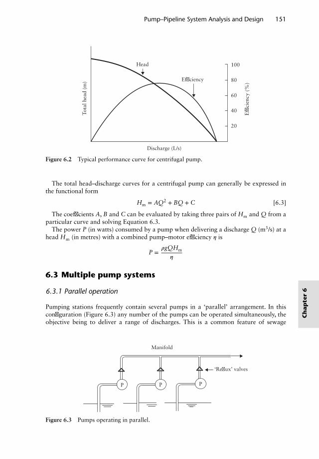
Pump–Pipeline System Analysis and Design 151
100
80
60
40
20
Efficiency
Effi
cien
cy (
%)
Tota
l hea
d (m
)
Head
Discharge (L/s)
Figure 6.2 Typical performance curve for centrifugal pump.
The total head–discharge curves for a centrifugal pump can generally be expressed inthe functional form
Hm = AQ2 + BQ + C [6.3]
The coefficients A, B and C can be evaluated by taking three pairs of Hm and Q from aparticular curve and solving Equation 6.3.
The power P (in watts) consumed by a pump when delivering a discharge Q (m3/s) at ahead Hm (in metres) with a combined pump–motor efficiency 𝜂 is
P =𝜌gQHm
𝜂
6.3 Multiple pump systems
6.3.1 Parallel operation
Pumping stations frequently contain several pumps in a ‘parallel’ arrangement. In thisconfiguration (Figure 6.3) any number of the pumps can be operated simultaneously, theobjective being to deliver a range of discharges. This is a common feature of sewage
Manifold
‘Reflux’ valves
PPP
Figure 6.3 Pumps operating in parallel.
Ch
apte
r6
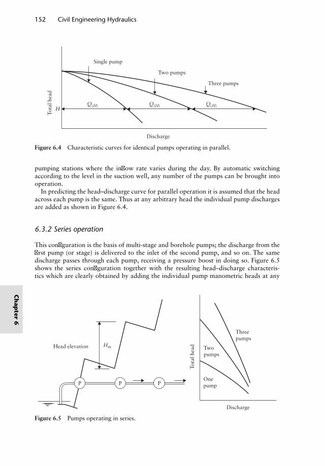
152 Civil Engineering Hydraulics
Single pump
Discharge
Tota
l hea
d
Two pumps
Three pumps
Q(H)Q(H)Q(H)H
Figure 6.4 Characteristic curves for identical pumps operating in parallel.
pumping stations where the inflow rate varies during the day. By automatic switchingaccording to the level in the suction well, any number of the pumps can be brought intooperation.
In predicting the head–discharge curve for parallel operation it is assumed that the headacross each pump is the same. Thus at any arbitrary head the individual pump dischargesare added as shown in Figure 6.4.
6.3.2 Series operation
This configuration is the basis of multi-stage and borehole pumps; the discharge from thefirst pump (or stage) is delivered to the inlet of the second pump, and so on. The samedischarge passes through each pump, receiving a pressure boost in doing so. Figure 6.5shows the series configuration together with the resulting head–discharge characteris-tics which are clearly obtained by adding the individual pump manometric heads at any
Threepumps
Twopumps
Onepump
Discharge
Head elevation Hm
Tota
l hea
d
PPP
Figure 6.5 Pumps operating in series.
Ch
apter
6
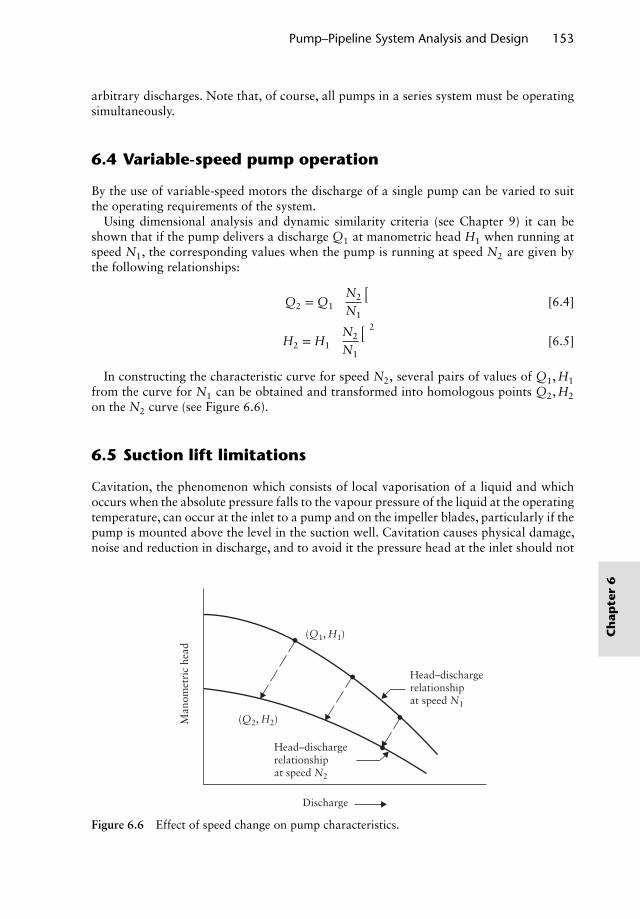
Pump–Pipeline System Analysis and Design 153
arbitrary discharges. Note that, of course, all pumps in a series system must be operatingsimultaneously.
6.4 Variable-speed pump operation
By the use of variable-speed motors the discharge of a single pump can be varied to suitthe operating requirements of the system.
Using dimensional analysis and dynamic similarity criteria (see Chapter 9) it can beshown that if the pump delivers a discharge Q1 at manometric head H1 when running atspeed N1, the corresponding values when the pump is running at speed N2 are given bythe following relationships:
Q2 = Q1
(N2
N1
)[6.4]
H2 = H1
(N2
N1
)2
[6.5]
In constructing the characteristic curve for speed N2, several pairs of values of Q1, H1from the curve for N1 can be obtained and transformed into homologous points Q2, H2on the N2 curve (see Figure 6.6).
6.5 Suction lift limitations
Cavitation, the phenomenon which consists of local vaporisation of a liquid and whichoccurs when the absolute pressure falls to the vapour pressure of the liquid at the operatingtemperature, can occur at the inlet to a pump and on the impeller blades, particularly if thepump is mounted above the level in the suction well. Cavitation causes physical damage,noise and reduction in discharge, and to avoid it the pressure head at the inlet should not
Man
omet
ric
head
Head–dischargerelationshipat speed N1
Head–dischargerelationshipat speed N2
(Q1, H1)
(Q2, H2)
Discharge
Figure 6.6 Effect of speed change on pump characteristics.
Ch
apte
r6
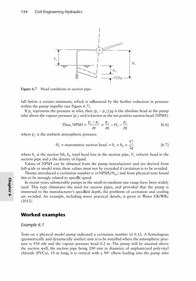
154 Civil Engineering Hydraulics
P
hs
hls
Vs2/2g
Hs
Figure 6.7 Head conditions in suction pipe.
fall below a certain minimum, which is influenced by the further reduction in pressurewithin the pump impeller (see Figure 6.7).
If ps represents the pressure at inlet, then (ps − pv)∕𝜌g is the absolute head at the pumpinlet above the vapour pressure (pv) and is known as the net positive suction head (NPSH).
Thus, NPSH =ps − pv
𝜌g=
pa
𝜌g− Hs −
pv
𝜌g[6.6]
where pa is the ambient atmospheric pressure.
Hs = manometric suction head = hs + hls +V2
s
2g[6.7]
where hs is the suction lift, hls total head loss in the suction pipe, Vs velocity head in thesuction pipe and 𝜌 the density of liquid.
Values of NPSH can be obtained from the pump manufacturer and are derived fromfull-scale or model tests; these values must not be exceeded if cavitation is to be avoided.
Thoma introduced a cavitation number 𝜎 (=NPSH∕Hm) and from physical tests foundthis to be strongly related to specific speed.
In recent years submersible pumps in the small-to-medium size range have been widelyused. This type eliminates the need for suction pipes, and provided that the pump isimmersed to the manufacturer’s specified depth, the problems of cavitation and coolingare avoided. An example, including many practical details, is given in Water UK/WRc(2012).
Worked examples
Example 6.1
Tests on a physical model pump indicated a cavitation number of 0.12. A homologous(geometrically and dynamically similar) unit is to be installed where the atmospheric pres-sure is 950 mb and the vapour pressure head 0.2 m. The pump will be situated abovethe suction well, the suction pipe being 200 mm in diameter, of unplasticised polyvinylchloride (PVCu), 10 m long; it is vertical with a 90◦ elbow leading into the pump inlet
Ch
apter
6
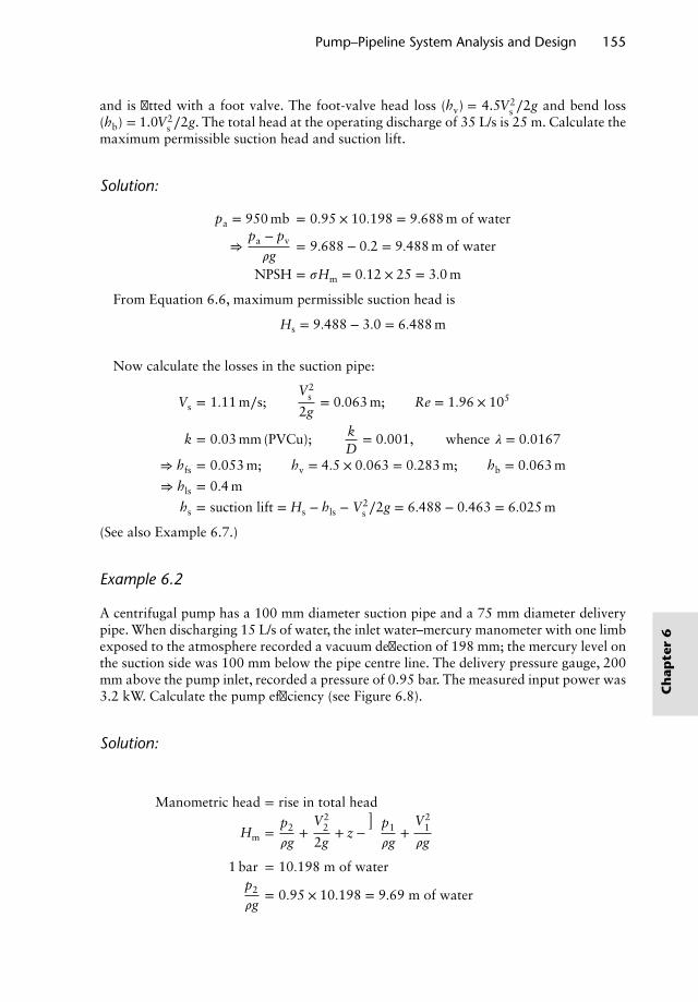
Pump–Pipeline System Analysis and Design 155
and is fitted with a foot valve. The foot-valve head loss (hv) = 4.5V2s ∕2g and bend loss
(hb) = 1.0V2s ∕2g. The total head at the operating discharge of 35 L/s is 25 m. Calculate the
maximum permissible suction head and suction lift.
Solution:
pa = 950 mb = 0.95 × 10.198 = 9.688 m of water
⇒pa − pv
𝜌g= 9.688 − 0.2 = 9.488 m of water
NPSH = 𝜎Hm = 0.12 × 25 = 3.0 m
From Equation 6.6, maximum permissible suction head is
Hs = 9.488 − 3.0 = 6.488 m
Now calculate the losses in the suction pipe:
Vs = 1.11 m∕s;V2
s
2g= 0.063 m; Re = 1.96 × 10⁵
k = 0.03 mm (PVCu); kD
= 0.001, whence 𝜆 = 0.0167
⇒ hfs = 0.053 m; hv = 4.5 × 0.063 = 0.283 m; hb = 0.063 m
⇒ hls = 0.4 m
hs = suction lift = Hs − hls − V2s ∕2g = 6.488 − 0.463 = 6.025 m
(See also Example 6.7.)
Example 6.2
A centrifugal pump has a 100 mm diameter suction pipe and a 75 mm diameter deliverypipe. When discharging 15 L/s of water, the inlet water–mercury manometer with one limbexposed to the atmosphere recorded a vacuum deflection of 198 mm; the mercury level onthe suction side was 100 mm below the pipe centre line. The delivery pressure gauge, 200mm above the pump inlet, recorded a pressure of 0.95 bar. The measured input power was3.2 kW. Calculate the pump efficiency (see Figure 6.8).
Solution:
Manometric head = rise in total head
Hm =p2
𝜌g+
V22
2g+ z −
(p1
𝜌g+
V21
𝜌g
)
1 bar = 10.198 m of waterp2
𝜌g= 0.95 × 10.198 = 9.69 m of water
Ch
apte
r6
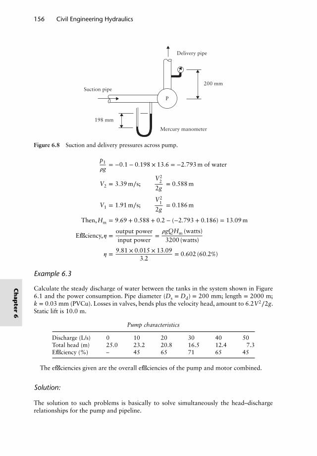
156 Civil Engineering Hydraulics
P
Mercury manometer
200 mm
198 mm
Delivery pipe
Suction pipe
Figure 6.8 Suction and delivery pressures across pump.
p1
𝜌g= −0.1 − 0.198 × 13.6 = −2.793 m of water
V2 = 3.39 m∕s;V2
2
2g= 0.588 m
V1 = 1.91 m∕s;V2
1
2g= 0.186 m
Then,Hm = 9.69 + 0.588 + 0.2 − (−2.793 + 0.186) = 13.09 m
Efficiency,𝜂 =output powerinput power
=𝜌gQHm (watts)
3200 (watts)
𝜂 = 9.81 × 0.015 × 13.093.2
= 0.602 (60.2%)
Example 6.3
Calculate the steady discharge of water between the tanks in the system shown in Figure6.1 and the power consumption. Pipe diameter (Ds = Dd) = 200 mm; length = 2000 m;k = 0.03 mm (PVCu). Losses in valves, bends plus the velocity head, amount to 6.2V2∕2g.Static lift is 10.0 m.
Pump characteristics
Discharge (L/s) 0 10 20 30 40 50Total head (m) 25.0 23.2 20.8 16.5 12.4 7.3Efficiency (%) – 45 65 71 65 45
The efficiencies given are the overall efficiencies of the pump and motor combined.
Solution:
The solution to such problems is basically to solve simultaneously the head–dischargerelationships for the pump and pipeline.
Ch
apter
6
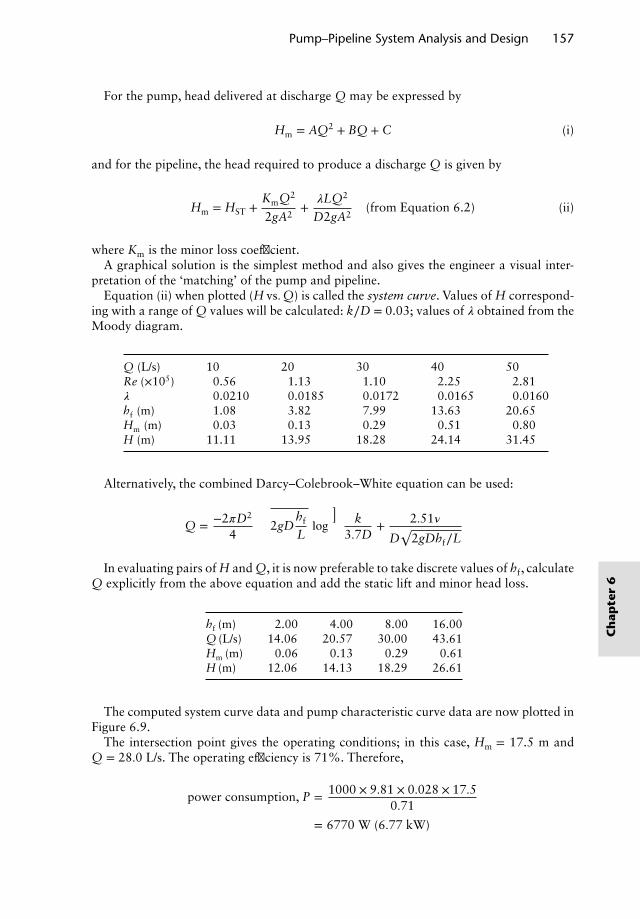
Pump–Pipeline System Analysis and Design 157
For the pump, head delivered at discharge Q may be expressed by
Hm = AQ2 + BQ + C (i)
and for the pipeline, the head required to produce a discharge Q is given by
Hm = HST +KmQ2
2gA2+𝜆LQ2
D2gA2(from Equation 6.2) (ii)
where Km is the minor loss coefficient.A graphical solution is the simplest method and also gives the engineer a visual inter-
pretation of the ‘matching’ of the pump and pipeline.Equation (ii) when plotted (H vs.Q) is called the system curve. Values of H correspond-
ing with a range of Q values will be calculated: k∕D = 0.03; values of 𝜆 obtained from theMoody diagram.
Q (L/s) 10 20 30 40 50Re (×105) 0.56 1.13 1.10 2.25 2.81𝜆 0.0210 0.0185 0.0172 0.0165 0.0160hf (m) 1.08 3.82 7.99 13.63 20.65Hm (m) 0.03 0.13 0.29 0.51 0.80H (m) 11.11 13.95 18.28 24.14 31.45
Alternatively, the combined Darcy–Colebrook–White equation can be used:
Q = −2𝜋D2
4
√2gD
hf
Llog
(k
3.7D+ 2.51𝜈
D√
2gDhf∕L
)
In evaluating pairs of H and Q, it is now preferable to take discrete values of hf, calculateQ explicitly from the above equation and add the static lift and minor head loss.
hf (m) 2.00 4.00 8.00 16.00Q (L/s) 14.06 20.57 30.00 43.61Hm (m) 0.06 0.13 0.29 0.61H (m) 12.06 14.13 18.29 26.61
The computed system curve data and pump characteristic curve data are now plotted inFigure 6.9.
The intersection point gives the operating conditions; in this case, Hm = 17.5 m andQ = 28.0 L/s. The operating efficiency is 71%. Therefore,
power consumption, P = 1000 × 9.81 × 0.028 × 17.50.71
= 6770 W (6.77 kW)
Ch
apte
r6
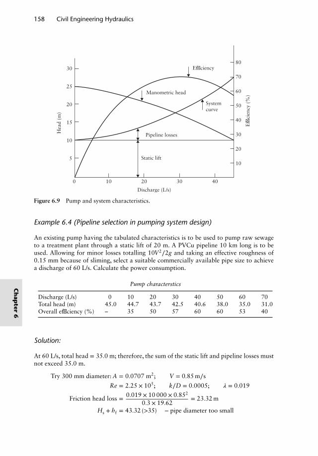
158 Civil Engineering Hydraulics
80
70
60
50
40
30
20
10
30
25
20
15
10
5
Hea
d (m
)
Discharge (L/s)
Static lift
Pipeline losses
Systemcurve
Efficiency
Manometric head
Effi
cien
cy (
%)
403020100
Figure 6.9 Pump and system characteristics.
Example 6.4 (Pipeline selection in pumping system design)
An existing pump having the tabulated characteristics is to be used to pump raw sewageto a treatment plant through a static lift of 20 m. A PVCu pipeline 10 km long is to beused. Allowing for minor losses totalling 10V2∕2g and taking an effective roughness of0.15 mm because of sliming, select a suitable commercially available pipe size to achievea discharge of 60 L/s. Calculate the power consumption.
Pump characterstics
Discharge (L/s) 0 10 20 30 40 50 60 70Total head (m) 45.0 44.7 43.7 42.5 40.6 38.0 35.0 31.0Overall efficiency (%) – 35 50 57 60 60 53 40
Solution:
At 60 L/s, total head = 35.0 m; therefore, the sum of the static lift and pipeline losses mustnot exceed 35.0 m.
Try 300 mm diameter: A = 0.0707 m2; V = 0.85 m∕s
Re = 2.25 × 10⁵; k∕D = 0.0005; 𝜆 = 0.019
Friction head loss = 0.019 × 10 000 × 0.852
0.3 × 19.62= 23.32 m
Hs + hf = 43.32 (>35) − pipe diameter too small
Ch
apter
6
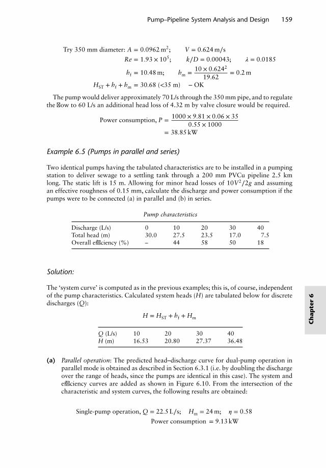
Pump–Pipeline System Analysis and Design 159
Try 350 mm diameter: A = 0.0962 m2; V = 0.624 m∕s
Re = 1.93 × 10⁵; k∕D = 0.00043; 𝜆 = 0.0185
hf = 10.48 m; hm = 10 × 0.6242
19.62= 0.2 m
HST + hf + hm = 30.68 (<35 m) − OK
The pump would deliver approximately 70 L/s through the 350 mm pipe, and to regulatethe flow to 60 L/s an additional head loss of 4.32 m by valve closure would be required.
Power consumption, P = 1000 × 9.81 × 0.06 × 350.55 × 1000
= 38.85 kW
Example 6.5 (Pumps in parallel and series)
Two identical pumps having the tabulated characteristics are to be installed in a pumpingstation to deliver sewage to a settling tank through a 200 mm PVCu pipeline 2.5 kmlong. The static lift is 15 m. Allowing for minor head losses of 10V2∕2g and assumingan effective roughness of 0.15 mm, calculate the discharge and power consumption if thepumps were to be connected (a) in parallel and (b) in series.
Pump characteristics
Discharge (L/s) 0 10 20 30 40Total head (m) 30.0 27.5 23.5 17.0 7.5Overall efficiency (%) – 44 58 50 18
Solution:
The ‘system curve’ is computed as in the previous examples; this is, of course, independentof the pump characteristics. Calculated system heads (H) are tabulated below for discretedischarges (Q):
H = HST + hf + Hm
Q (L/s) 10 20 30 40H (m) 16.53 20.80 27.37 36.48
(a) Parallel operation: The predicted head–discharge curve for dual-pump operation inparallel mode is obtained as described in Section 6.3.1 (i.e. by doubling the dischargeover the range of heads, since the pumps are identical in this case). The system andefficiency curves are added as shown in Figure 6.10. From the intersection of thecharacteristic and system curves, the following results are obtained:
Single-pump operation, Q = 22.5 L∕s; Hm = 24 m; 𝜂 = 0.58
Power consumption = 9.13 kW
Ch
apte
r6
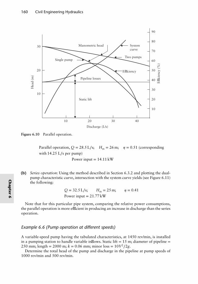
160 Civil Engineering Hydraulics
90
80
70
60
50
40
30
20
10
30
20
10
Hea
d (m
)
Discharge (L/s)
Static lift
Pipeline losses
Systemcurve
Two pumpsSingle pump
Efficiency
Manometric head
Effi
cien
cy (
%)
10 20 30 40
Figure 6.10 Parallel operation.
Parallel operation, Q = 28.5 L∕s; Hm = 26 m; 𝜂 = 0.51 (corresponding
with 14.25 L∕s per pump)
Power input = 14.11 kW
(b) Series operation: Using the method described in Section 6.3.2 and plotting the dual-pump characteristic curve, intersection with the system curve yields (see Figure 6.11)the following:
Q = 32.5 L∕s; Hm = 25 m; 𝜂 = 0.41
Power input = 21.77 kW
Note that for this particular pipe system, comparing the relative power consumptions,the parallel operation is more efficient in producing an increase in discharge than the seriesoperation.
Example 6.6 (Pump operation at different speeds)
A variable-speed pump having the tabulated characteristics, at 1450 rev/min, is installedin a pumping station to handle variable inflows. Static lift = 15 m; diameter of pipeline =250 mm; length = 2000 m; k = 0.06 mm; minor loss = 10V2∕2g.
Determine the total head of the pump and discharge in the pipeline at pump speeds of1000 rev/min and 500 rev/min.
Ch
apter
6
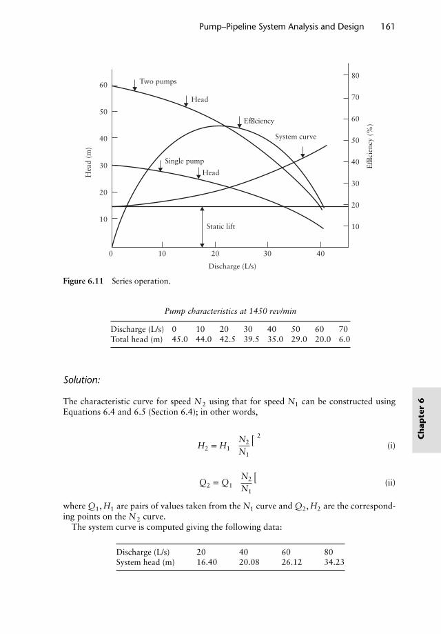
Pump–Pipeline System Analysis and Design 161
80
70
60
50
40
30
20
10
60
50
40
30
20
10
Hea
d (m
)
Discharge (L/s)
Static lift
Single pump
Head
Head
Two pumps
System curve
Efficiency
Effi
cien
cy (
%)
0 10 20 30 40
Figure 6.11 Series operation.
Pump characteristics at 1450 rev/min
Discharge (L/s) 0 10 20 30 40 50 60 70Total head (m) 45.0 44.0 42.5 39.5 35.0 29.0 20.0 6.0
Solution:
The characteristic curve for speed N 2 using that for speed N1 can be constructed usingEquations 6.4 and 6.5 (Section 6.4); in other words,
H2 = H1
(N2
N1
)2
(i)
Q2 = Q1
(N2
N1
)(ii)
where Q1, H1 are pairs of values taken from the N1 curve and Q2, H2 are the correspond-ing points on the N2 curve.
The system curve is computed giving the following data:
Discharge (L/s) 20 40 60 80System head (m) 16.40 20.08 26.12 34.23
Ch
apte
r6
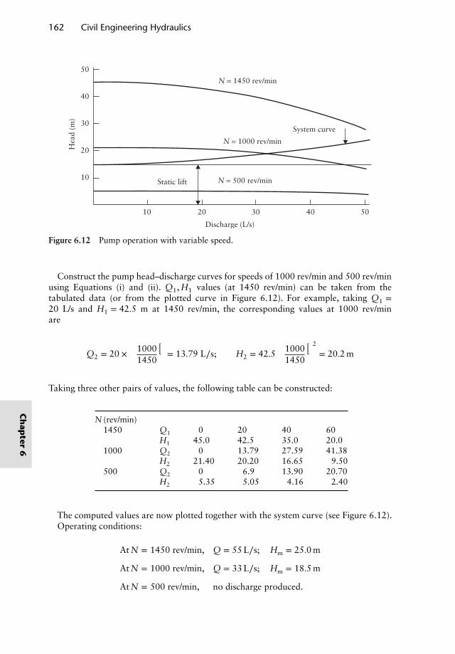
162 Civil Engineering Hydraulics
50
40
30
20
10
Hea
d (m
)
Discharge (L/s)
System curve
Static lift
N = 1450 rev/min
N = 1000 rev/min
N = 500 rev/min
10 20 30 40 50
Figure 6.12 Pump operation with variable speed.
Construct the pump head–discharge curves for speeds of 1000 rev/min and 500 rev/minusing Equations (i) and (ii). Q1, H1 values (at 1450 rev/min) can be taken from thetabulated data (or from the plotted curve in Figure 6.12). For example, taking Q1 =20 L/s and H1 = 42.5 m at 1450 rev/min, the corresponding values at 1000 rev/minare
Q2 = 20 ×(
10001450
)= 13.79 L∕s; H2 = 42.5
(10001450
)2
= 20.2 m
Taking three other pairs of values, the following table can be constructed:
N (rev/min)1450 Q1 0 20 40 60
H1 45.0 42.5 35.0 20.01000 Q2 0 13.79 27.59 41.38
H2 21.40 20.20 16.65 9.50500 Q2 0 6.9 13.90 20.70
H2 5.35 5.05 4.16 2.40
The computed values are now plotted together with the system curve (see Figure 6.12).Operating conditions:
At N = 1450 rev/min, Q = 55 L∕s; Hm = 25.0 m
At N = 1000 rev/min, Q = 33 L∕s; Hm = 18.5 m
At N = 500 rev/min, no discharge produced.
Ch
apter
6
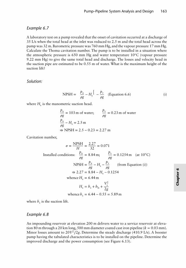
Pump–Pipeline System Analysis and Design 163
Example 6.7
A laboratory test on a pump revealed that the onset of cavitation occurred at a discharge of35 L/s when the total head at the inlet was reduced to 2.5 m and the total head across thepump was 32 m. Barometric pressure was 760 mm Hg, and the vapour pressure 17 mm Hg.Calculate the Thoma cavitation number. The pump is to be installed in a situation wherethe atmospheric pressure is 650 mm Hg and water temperature 10◦C (vapour pressure9.22 mm Hg) to give the same total head and discharge. The losses and velocity head inthe suction pipe are estimated to be 0.55 m of water. What is the maximum height of thesuction lift?
Solution:
NPSH =(
pa
𝜌g− Hs
)−
pv
𝜌g(Equation 6.6) (i)
where Hs is the manometric suction head.
pa
𝜌g= 103 m of water;
pv
𝜌g= 0.23 m of water
pa
𝜌g− Hs = 2.5 m
⇒ NPSH = 2.5 − 0.23 = 2.27 m
Cavitation number,
𝜎 = NPSHH
= 2.2732
= 0.071
Installed conditions:pa
𝜌g= 8.84 m;
pv
𝜌g= 0.1254 m (at 10◦C)
NPSH =pa
𝜌g− Hs −
pv
𝜌g(from Equation (i))
⇒ 2.27 = 8.84 − Hs − 0.1254
whence Hs = 6.44 m
Hs = hs + hls +V2
s
2gwhence hs = 6.44 − 0.55 = 5.89 m
where hs is the suction lift.
Example 6.8
An impounding reservoir at elevation 200 m delivers water to a service reservoir at eleva-tion 80 m through a 20 km long, 500 mm diameter coated cast iron pipeline (k = 0.03 mm).Minor losses amount to 20V2∕2g. Determine the steady discharge (410.9 L/s). A boosterpump having the tabulated characteristics is to be installed on the pipeline. Determine theimproved discharge and the power consumption (see Figure 6.13).
Ch
apte
r6
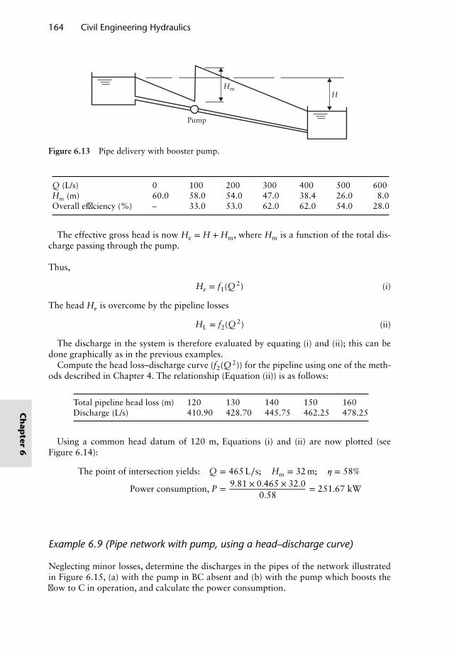
164 Civil Engineering Hydraulics
HmH
Pump
Figure 6.13 Pipe delivery with booster pump.
Q (L/s) 0 100 200 300 400 500 600Hm (m) 60.0 58.0 54.0 47.0 38.4 26.0 8.0Overall efficiency (%) – 33.0 53.0 62.0 62.0 54.0 28.0
The effective gross head is now He = H + Hm, where Hm is a function of the total dis-charge passing through the pump.
Thus,
He = f1(Q 2) (i)
The head He is overcome by the pipeline losses
HL = f2(Q 2) (ii)
The discharge in the system is therefore evaluated by equating (i) and (ii); this can bedone graphically as in the previous examples.
Compute the head loss–discharge curve (f2(Q 2)) for the pipeline using one of the meth-ods described in Chapter 4. The relationship (Equation (ii)) is as follows:
Total pipeline head loss (m) 120 130 140 150 160Discharge (L/s) 410.90 428.70 445.75 462.25 478.25
Using a common head datum of 120 m, Equations (i) and (ii) are now plotted (seeFigure 6.14):
The point of intersection yields: Q = 465 L∕s; Hm = 32 m; 𝜂 = 58%
Power consumption, P = 9.81 × 0.465 × 32.00.58
= 251.67 kW
Example 6.9 (Pipe network with pump, using a head–discharge curve)
Neglecting minor losses, determine the discharges in the pipes of the network illustratedin Figure 6.15, (a) with the pump in BC absent and (b) with the pump which boosts theflow to C in operation, and calculate the power consumption.
Ch
apter
6
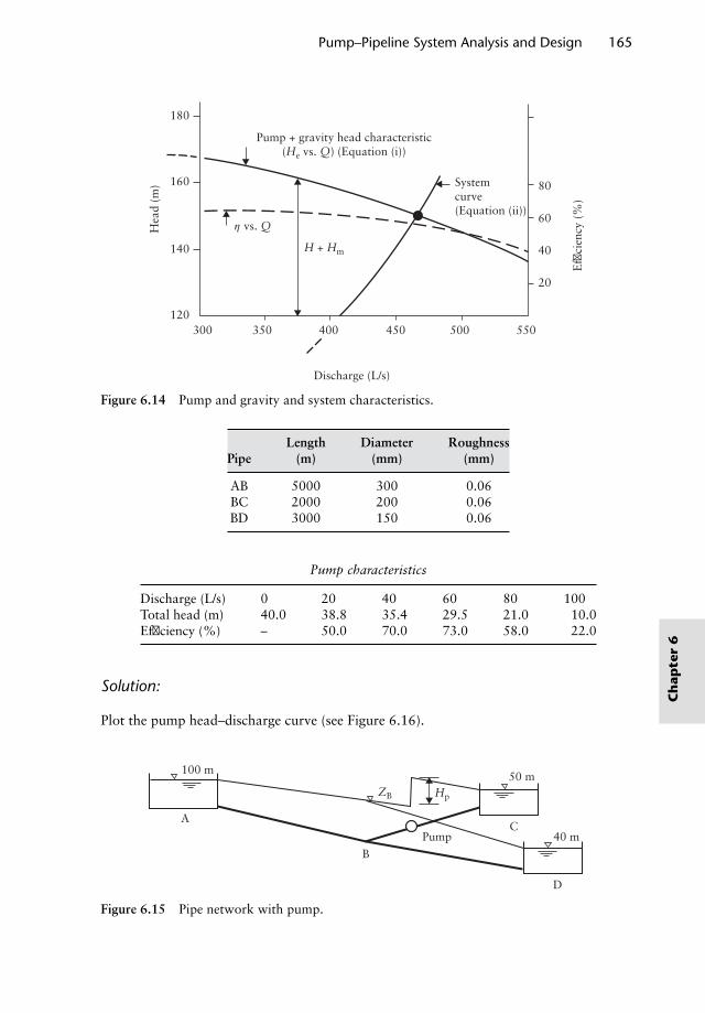
Pump–Pipeline System Analysis and Design 165
Hea
d (m
)
Discharge (L/s)
Systemcurve(Equation (ii))
80
60
40
20
Pump + gravity head characteristic(He vs. Q) (Equation (i))
H + Hm
η vs. Q
300 350
180
160
140
120400 450 500 550
Effi
cien
cy (
%)
Figure 6.14 Pump and gravity and system characteristics.
Length Diameter RoughnessPipe (m) (mm) (mm)
AB 5000 300 0.06BC 2000 200 0.06BD 3000 150 0.06
Pump characteristics
Discharge (L/s) 0 20 40 60 80 100Total head (m) 40.0 38.8 35.4 29.5 21.0 10.0Efficiency (%) – 50.0 70.0 73.0 58.0 22.0
Solution:
Plot the pump head–discharge curve (see Figure 6.16).
HpZB
40 m
D
50 m100 m
AC
Pump
B
Figure 6.15 Pipe network with pump.
Ch
apte
r6
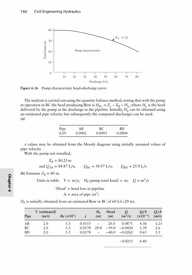
166 Civil Engineering Hydraulics
40
30
20
10
08070605040302010
Discharge (L/s)
Tota
l hea
d (m
)
Pump characteristics
Hm vs. Q
Figure 6.16 Pump characteristic head–discharge curve.
The analysis is carried out using the quantity balance method, noting that with the pumpin operation in BC the head producing flow is HBC = Zc − ZB − Hp, where Hp is the headdelivered by the pump at the discharge in the pipeline. Initially, Hp can be obtained usingan estimated pipe velocity but subsequently the computed discharges can be used.(a)
Pipe AB BC BDk∕D 0.0002 0.0003 0.0004
𝜆 values may be obtained from the Moody diagram using initially assumed values ofpipe velocity.
With the pump not installed,
ZB = 80.25 m
and QAB = 84.87 L∕s; QBC = 58.97 L∕s; QBD = 25.9 L∕s
(b) Estimate ZB = 80 m.
Units in table: V = m∕s; HP (pump total head) = m; Q = m3∕s
‘Head’ = head loss in pipeline
A = area of pipe (m2)
HP is initially obtained from an estimated flow in BC of 60 L/s (29 m).
V (estimated) HP Head Q Q∕h Q∕APipe (m/s) Re (×105) 𝝀 (m) (m) (m3/s) (×10−3) (m/s)
AB 2.0 5.3 0.0155 – 20.0 0.0871 4.36 1.23BC 2.0 5.3 0.0170 29.0 −59.0 −0.0820 1.39 2.6BD 2.0 5.3 0.0178 – −40.0 −0.0262 0.65 1.5
∑−0.0211 6.40
Ch
apter
6
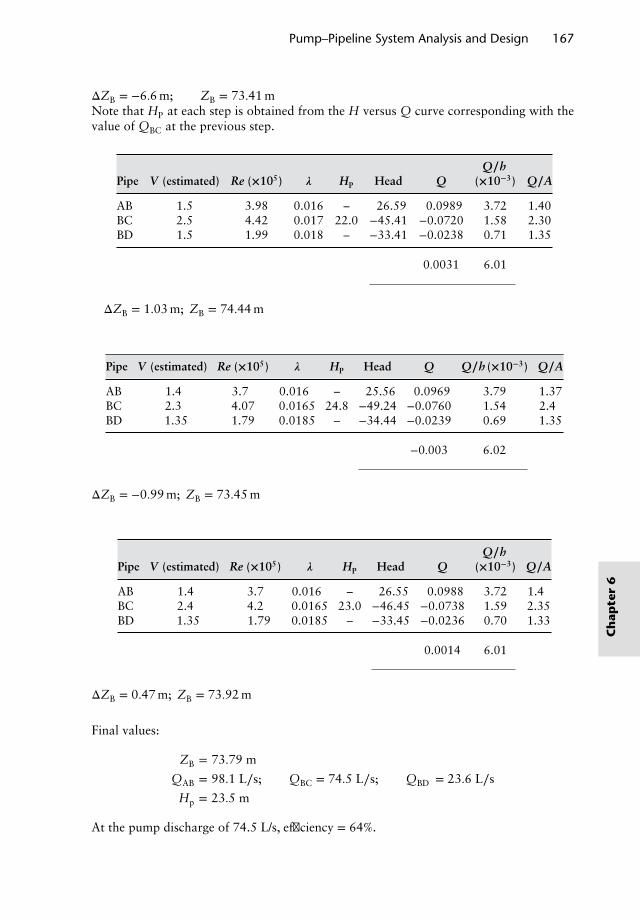
Pump–Pipeline System Analysis and Design 167
ΔZB = −6.6 m; ZB = 73.41 mNote that HP at each step is obtained from the H versus Q curve corresponding with thevalue of QBC at the previous step.
Q∕hPipe V (estimated) Re (×105) 𝝀 HP Head Q (×10−3) Q∕A
AB 1.5 3.98 0.016 – 26.59 0.0989 3.72 1.40BC 2.5 4.42 0.017 22.0 −45.41 −0.0720 1.58 2.30BD 1.5 1.99 0.018 – −33.41 −0.0238 0.71 1.35
∑0.0031 6.01
ΔZB = 1.03 m; ZB = 74.44 m
Pipe V (estimated) Re (×105) 𝝀 HP Head Q Q∕h (×10−3) Q∕A
AB 1.4 3.7 0.016 – 25.56 0.0969 3.79 1.37BC 2.3 4.07 0.0165 24.8 −49.24 −0.0760 1.54 2.4BD 1.35 1.79 0.0185 – −34.44 −0.0239 0.69 1.35
∑−0.003 6.02
ΔZB = −0.99 m; ZB = 73.45 m
Q∕hPipe V (estimated) Re (×105) 𝝀 HP Head Q (×10−3) Q∕A
AB 1.4 3.7 0.016 – 26.55 0.0988 3.72 1.4BC 2.4 4.2 0.0165 23.0 −46.45 −0.0738 1.59 2.35BD 1.35 1.79 0.0185 – −33.45 −0.0236 0.70 1.33
∑0.0014 6.01
ΔZB = 0.47 m; ZB = 73.92 m
Final values:
ZB = 73.79 m
QAB = 98.1 L∕s; QBC = 74.5 L∕s; QBD = 23.6 L∕s
Hp = 23.5 m
At the pump discharge of 74.5 L/s, efficiency = 64%.
Ch
apte
r6
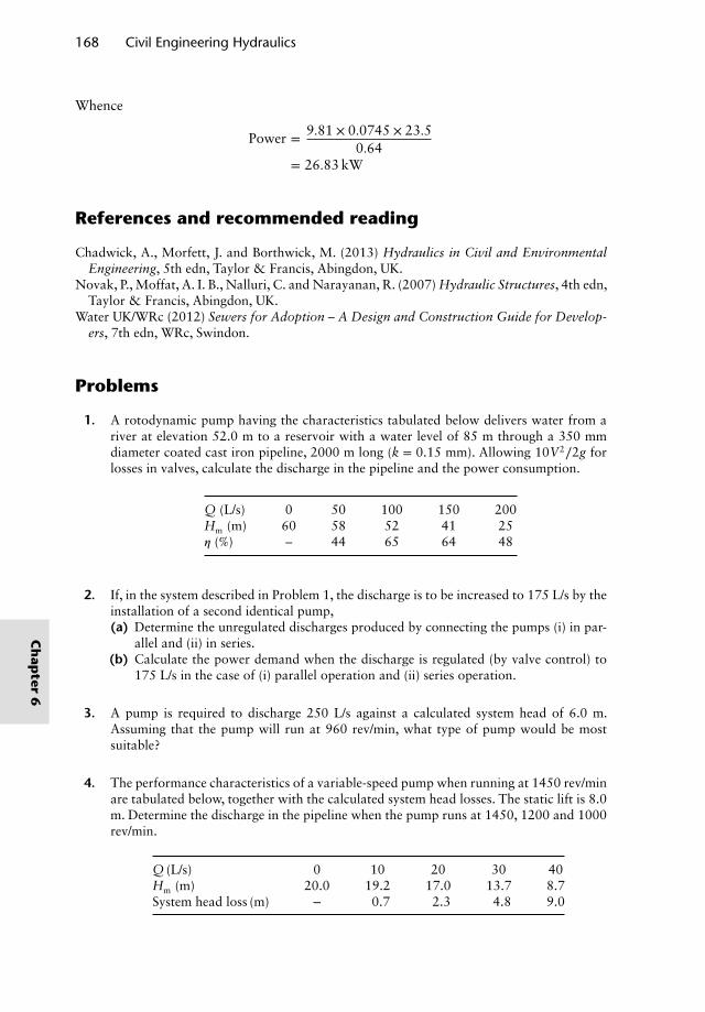
168 Civil Engineering Hydraulics
Whence
Power = 9.81 × 0.0745 × 23.50.64
= 26.83 kW
References and recommended reading
Chadwick, A., Morfett, J. and Borthwick, M. (2013) Hydraulics in Civil and EnvironmentalEngineering, 5th edn, Taylor & Francis, Abingdon, UK.
Novak, P., Moffat, A. I. B., Nalluri, C. and Narayanan, R. (2007) Hydraulic Structures, 4th edn,Taylor & Francis, Abingdon, UK.
Water UK/WRc (2012) Sewers for Adoption – A Design and Construction Guide for Develop-ers, 7th edn, WRc, Swindon.
Problems
1. A rotodynamic pump having the characteristics tabulated below delivers water from ariver at elevation 52.0 m to a reservoir with a water level of 85 m through a 350 mmdiameter coated cast iron pipeline, 2000 m long (k = 0.15 mm). Allowing 10V2∕2g forlosses in valves, calculate the discharge in the pipeline and the power consumption.
Q (L/s) 0 50 100 150 200Hm (m) 60 58 52 41 25𝜂 (%) – 44 65 64 48
2. If, in the system described in Problem 1, the discharge is to be increased to 175 L/s by theinstallation of a second identical pump,(a) Determine the unregulated discharges produced by connecting the pumps (i) in par-
allel and (ii) in series.(b) Calculate the power demand when the discharge is regulated (by valve control) to
175 L/s in the case of (i) parallel operation and (ii) series operation.
3. A pump is required to discharge 250 L/s against a calculated system head of 6.0 m.Assuming that the pump will run at 960 rev/min, what type of pump would be mostsuitable?
4. The performance characteristics of a variable-speed pump when running at 1450 rev/minare tabulated below, together with the calculated system head losses. The static lift is 8.0m. Determine the discharge in the pipeline when the pump runs at 1450, 1200 and 1000rev/min.
Q (L/s) 0 10 20 30 40Hm (m) 20.0 19.2 17.0 13.7 8.7System head loss (m) − 0.7 2.3 4.8 9.0
Ch
apter
6
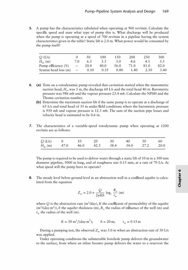
Pump–Pipeline System Analysis and Design 169
5. A pump has the characteristics tabulated when operating at 960 rev/min. Calculate thespecific speed and state what type of pump this is. What discharge will be producedwhen the pump is operating at a speed of 700 rev/min in a pipeline having the systemcharacteristics given in the table? Static lift is 2.0 m. What power would be consumed bythe pump itself?
Q (L/s) 0 50 100 150 200 250 300Hm (m) 7.0 6.3 5.5 5.0 4.6 4.1 3.5Pump efficiency (%) − 20.0 40.0 56.0 71.0 81.0 82.0System head loss (m) − 0.10 0.35 0.80 1.40 2.10 3.40
6. (a) Tests on a rotodynamic pump revealed that cavitation started when the manometricsuction head, Hs, was 5 m, the discharge 60 L/s and the total head 40 m. Barometricpressure was 986 mb and the vapour pressure 23.4 mb. Calculate the NPSH and theThoma cavitation number.
(b) Determine the maximum suction lift if the same pump is to operate at a discharge of65 L/s and total head of 35 m under field conditions where the barometric pressureis 950 mb and vapour pressure is 12.5 mb. The sum of the suction pipe losses andvelocity head is estimated to be 0.6 m.
7. The characteristics of a variable-speed rotodynamic pump when operating at 1200rev/min are as follows:
Q (L/s) 0 10 20 30 40 50 60Hm (m) 47.0 46.0 42.5 38.4 34.0 27.2 20.0
The pump is required to be used to deliver water through a static lift of 10 m in a 300 mmdiameter pipeline, 5000 m long, and of roughness size 0.15 mm, at a rate of 70 L/s. Atwhat speed will the pump have to operate?
8. The steady level below ground level in an abstraction well in a confined aquifer is calcu-lated from the equation
Zw = 2.0 +Q
2𝜋Kbloge
Ro
rw(m)
where Q is the abstraction rate (m3/day), K the coefficient of permeability of the aquifer(m3/(day m2)), b the aquifer thickness (m), Ro the radius of influence of the well (m) andrw the radius of the well (m).
K = 50 m3∕(day m2); b = 20 m; rw = 0.15 m
During a pumping test, the observed Zw was 5.0 m when an abstraction rate of 30 L/swas applied.
Under operating conditions the submersible borehole pump delivers the groundwaterto the surface, from where an inline booster pump delivers the water to a reservoir the
Ch
apte
r6
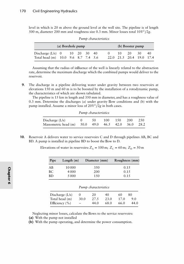
170 Civil Engineering Hydraulics
level in which is 20 m above the ground level at the well site. The pipeline is of length500 m, diameter 200 mm and roughness size 0.3 mm. Minor losses total 10V2∕2g.
Pump characteristics
(a) Borehole pump (b) Booster pump
Discharge (L/s) 0 10 20 30 40 0 10 20 30 40Total head (m) 10.0 9.6 8.7 7.4 5.6 22.0 21.5 20.4 19.0 17.4
Assuming that the radius of influence of the well is linearly related to the abstractionrate, determine the maximum discharge which the combined pumps would deliver to thereservoir.
9. The discharge in a pipeline delivering water under gravity between two reservoirs atelevations 150 m and 60 m is to be boosted by the installation of a rotodynamic pump,the characteristics of which are shown tabulated.
The pipeline is 15 km in length and 350 mm in diameter, and has a roughness value of0.3 mm. Determine the discharges (a) under gravity flow conditions and (b) with thepump installed. Assume a minor loss of 20V2∕2g in both cases.
Pump characteristics
Discharge (L/s) 0 50 100 150 200 250Manometric head (m) 50.0 49.0 46.5 42.0 36.0 28.2
10. Reservoir A delivers water to service reservoirs C and D through pipelines AB, BC andBD. A pump is installed in pipeline BD to boost the flow to D.
Elevations of water in reservoirs: ZA = 100 m; ZC = 60 m; ZD = 50 m
Pipe Length (m) Diameter (mm) Roughness (mm)
AB 10 000 350 0.15BC 4 000 200 0.15BD 5 000 150 0.15
Pump characteristics
Discharge (L/s) 0 20 40 60 80Total head (m) 30.0 27.5 23.0 17.0 9.0Efficiency (%) − 44.0 68.0 66.0 44.0
Neglecting minor losses, calculate the flows to the service reservoirs:(a) With the pump not installed(b) With the pump operating, and determine the power consumption.
Ch
apter
6
Chapter 7Boundary Layers on FlatPlates and in Ducts
7.1 Introduction
A boundary layer will develop along either side of a flat plate placed edgewise into a fluidstream (Figure 7.1) with free stream velocity U0 and kinematic viscosity 𝜈. Initially theflow in the layer may be laminar with a parabolic velocity distribution. The boundarylayer increases in thickness with distance x along the plate, and at a Reynolds numberU0x∕𝜈 ≃ 500 000 turbulence develops in the boundary layer. The frictional force due tothe turbulent portion of the boundary layer may be considered as that which would befound if the entire length were turbulent minus that corresponding to the hypotheticalturbulent layer up to the critical point.
For rough plates, Schlichting gave an expression for the maximum height of roughnesselements such that the surface may be considered hydraulically smooth:
k ≤ 100𝜈U0
[7.1]
The theory of boundary layers on smooth flat plates is to be found in texts such as Masseyand Ward-Smith (2012).
7.2 The laminar boundary layer
Blasius developed analytical equations for the flow in a laminar boundary layer formedon a flat plate for the case of zero pressure gradient along the plate. Taking the outer limitof the boundary layer as the position where v = 0.99U0, the boundary layer thickness 𝛿xat distance x from the leading edge was given as
𝛿x = 5x
Re1∕2x
where Rex =U0x𝜈
[7.2]
Local boundary shear stress, 𝜏0 = 0.332𝜇U0
xRe1∕2
x [7.3]
Nalluri & Featherstone’s Civil Engineering Hydraulics: Essential Theory with Worked Examples,Sixth Edition. Martin Marriott.© 2016 John Wiley & Sons, Ltd. Published 2016 by John Wiley & Sons, Ltd.Companion Website: www.wiley.com/go/Marriott
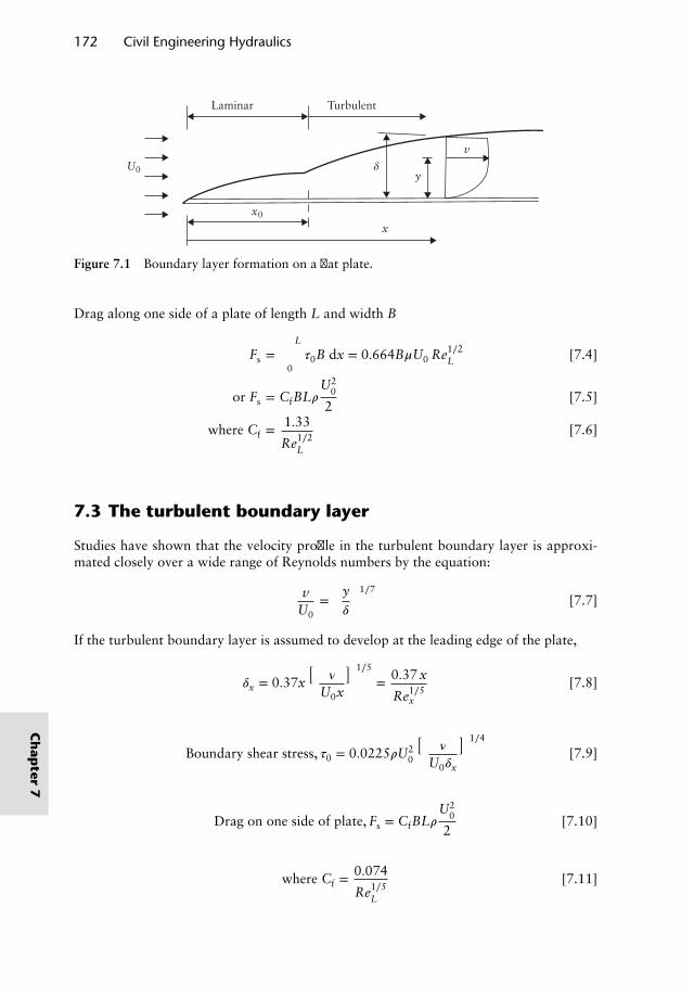
172 Civil Engineering Hydraulics
Laminar Turbulent
y
x
x0
U0
v
δ
Figure 7.1 Boundary layer formation on a flat plate.
Drag along one side of a plate of length L and width B
Fs = ∫L
0𝜏0B dx = 0.664B𝜇U0 Re1∕2
L [7.4]
or Fs = CfBL𝜌U2
0
2[7.5]
where Cf =1.33
Re1∕2L
[7.6]
7.3 The turbulent boundary layer
Studies have shown that the velocity profile in the turbulent boundary layer is approxi-mated closely over a wide range of Reynolds numbers by the equation:
vU0
=(y𝛿
)1∕7[7.7]
If the turbulent boundary layer is assumed to develop at the leading edge of the plate,
𝛿x = 0.37x(
𝜈
U0x
)1∕5
= 0.37 x
Re1∕5x
[7.8]
Boundary shear stress, 𝜏0 = 0.0225𝜌U20
(𝜈
U0𝛿x
)1∕4
[7.9]
Drag on one side of plate, Fs = CfBL𝜌U2
0
2[7.10]
where Cf =0.074
Re1∕5L
[7.11]
Ch
apter
7
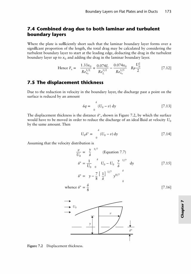
Boundary Layers on Flat Plates and in Ducts 173
7.4 Combined drag due to both laminar and turbulentboundary layers
Where the plate is sufficiently short such that the laminar boundary layer forms over asignificant proportion of the length, the total drag may be calculated by considering theturbulent boundary layer to start at the leading edge, deducting the drag in the turbulentboundary layer up to x0 and adding the drag in the laminar boundary layer.
Hence Fs =
(1.33x0
Re1∕2x0
+ 0.074L
Re1∕2L
−0.074x0
Re1∕5x0
)B𝜌
U20
2[7.12]
7.5 The displacement thickness
Due to the reduction in velocity in the boundary layer, the discharge past a point on thesurface is reduced by an amount
𝛿q = ∫𝛿
0(U0 − v) dy [7.13]
The displacement thickness is the distance 𝛿∗, shown in Figure 7.2, by which the surfacewould have to be moved in order to reduce the discharge of an ideal fluid at velocity U0by the same amount. Then
U0𝛿∗ = ∫
𝛿
0(U0 − v) dy [7.14]
Assuming that the velocity distribution is
vU0
=(y𝛿
)1∕7(Equation 7.7)
𝛿∗ = 1U0 ∫
𝛿
0
[U0 − U0
(y𝛿
)1∕7]
dy [7.15]
𝛿∗ =
[y − 7
8
(1𝛿
)1∕7
y8∕7
]𝛿0
whence 𝛿∗ = 𝛿
8[7.16]
y
U0
v
δ*
Figure 7.2 Displacement thickness.
Ch
apte
r7
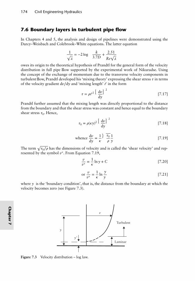
174 Civil Engineering Hydraulics
7.6 Boundary layers in turbulent pipe flow
In Chapters 4 and 5, the analysis and design of pipelines were demonstrated using theDarcy–Weisbach and Colebrook–White equations. The latter equation
1√𝜆= −2 log
(k
3.7D+ 2.51
Re√𝜆
)
owes its origin to the theoretical hypothesis of Prandtl for the general form of the velocitydistribution in full pipe flow supported by the experimental work of Nikuradse. Usingthe concept of the exchange of momentum due to the transverse velocity components inturbulent flow, Prandtl developed his ‘mixing theory’ expressing the shear stress 𝜏 in termsof the velocity gradient dv∕dy and ‘mixing length’ 𝓁 in the form
𝜏 = 𝜌𝓁2(
dvdy
)2
[7.17]
Prandtl further assumed that the mixing length was directly proportional to the distancefrom the boundary and that the shear stress was constant and hence equal to the boundaryshear stress 𝜏0. Hence,
𝜏0 = 𝜌(𝜅y)2(
dvdy
)2
[7.18]
whence dvdy
= 1𝜅
√𝜏0
𝜌
1y
[7.19]
The term√𝜏0∕𝜌 has the dimensions of velocity and is called the ‘shear velocity’ and rep-
resented by the symbol v∗. From Equation 7.19,
vv∗
= 1𝜅
ln y + C [7.20]
or vv∗
= 1𝜅
lnyy′
[7.21]
where y′ is the ‘boundary condition’, that is, the distance from the boundary at which thevelocity becomes zero (see Figure 7.3).
Laminar
Turbulent
y
v
y
Figure 7.3 Velocity distribution – log law.
Ch
apter
7
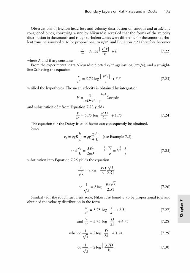
Boundary Layers on Flat Plates and in Ducts 175
Observations of friction head loss and velocity distribution on smooth and artificiallyroughened pipes, conveying water, by Nikuradse revealed that the forms of the velocitydistribution in the smooth and rough turbulent zones were different. For the smooth turbu-lent zone he assumed y′ to be proportional to v∕v∗, and Equation 7.21 therefore becomes
vv∗
= A log(
v∗y𝜈
)+ B [7.22]
where A and B are constants.From the experimental data Nikuradse plotted 𝜈∕v∗ against log (v∗y∕𝜈), and a straight-
line fit having the equation
𝜈
v∗= 5.75 log
(v∗y𝜈
)+ 5.5 [7.23]
verified the hypotheses. The mean velocity is obtained by integration
V = 1𝜋D2∕4 ∫
D∕2
02𝜋rv dr
and substitution of v from Equation 7.23 yields
Vv∗
= 5.75 log(v∗D
2𝜈
)+ 1.75 [7.24]
The equation for the Darcy friction factor can consequently be obtained.Since
𝜏0 = 𝜌gRhf
L= 𝜌g
D4
hf
L(see Example 7.5)
andhf
L= 𝜆V2
2gD;
√𝜏0
𝜌= V
√𝜆
8[7.25]
substitution into Equation 7.25 yields the equation
1√𝜆= 2 log
(VD𝜈
√𝜆
2.51
)
or 1√𝜆= 2 log
(Re
√𝜆
2.51
)[7.26]
Similarly for the rough turbulent zone, Nikuradse found y′ to be proportional to k andobtained the velocity distribution in the form
vv∗
= 5.75 log( y
k
)+ 8.5 [7.27]
and Vv∗
= 5.75 log( D
2k
)+ 4.75 [7.28]
whence 1√𝜆= 2 log
( D2k
)+ 1.74 [7.29]
or 1√𝜆= 2 log
(3.7D
k
)[7.30]
Ch
apte
r7
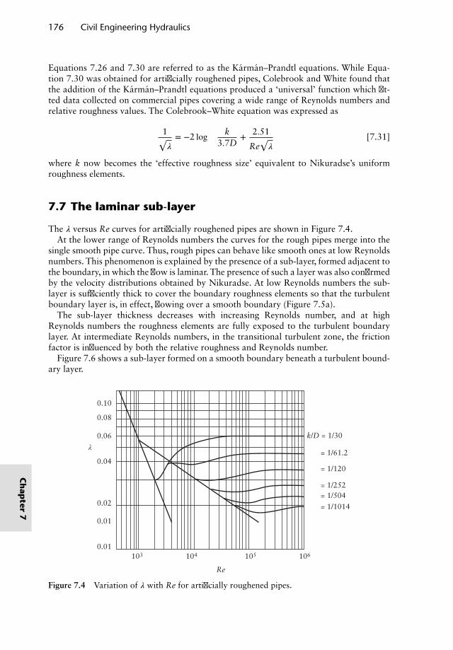
176 Civil Engineering Hydraulics
Equations 7.26 and 7.30 are referred to as the Karman–Prandtl equations. While Equa-tion 7.30 was obtained for artificially roughened pipes, Colebrook and White found thatthe addition of the Karman–Prandtl equations produced a ‘universal’ function which fit-ted data collected on commercial pipes covering a wide range of Reynolds numbers andrelative roughness values. The Colebrook–White equation was expressed as
1√𝜆= −2 log
(k
3.7D+ 2.51
Re√𝜆
)[7.31]
where k now becomes the ‘effective roughness size’ equivalent to Nikuradse’s uniformroughness elements.
7.7 The laminar sub-layer
The 𝜆 versus Re curves for artificially roughened pipes are shown in Figure 7.4.At the lower range of Reynolds numbers the curves for the rough pipes merge into the
single smooth pipe curve. Thus, rough pipes can behave like smooth ones at low Reynoldsnumbers. This phenomenon is explained by the presence of a sub-layer, formed adjacent tothe boundary, in which the flow is laminar. The presence of such a layer was also confirmedby the velocity distributions obtained by Nikuradse. At low Reynolds numbers the sub-layer is sufficiently thick to cover the boundary roughness elements so that the turbulentboundary layer is, in effect, flowing over a smooth boundary (Figure 7.5a).
The sub-layer thickness decreases with increasing Reynolds number, and at highReynolds numbers the roughness elements are fully exposed to the turbulent boundarylayer. At intermediate Reynolds numbers, in the transitional turbulent zone, the frictionfactor is influenced by both the relative roughness and Reynolds number.
Figure 7.6 shows a sub-layer formed on a smooth boundary beneath a turbulent bound-ary layer.
0.10
0.08
0.06
0.04
0.02
0.01
103 104 105 106
Re
k/D = 1/30
= 1/61.2
= 1/120
= 1/252= 1/504
= 1/1014
λ
0.01
Figure 7.4 Variation of 𝜆 with Re for artificially roughened pipes.
Ch
apter
7
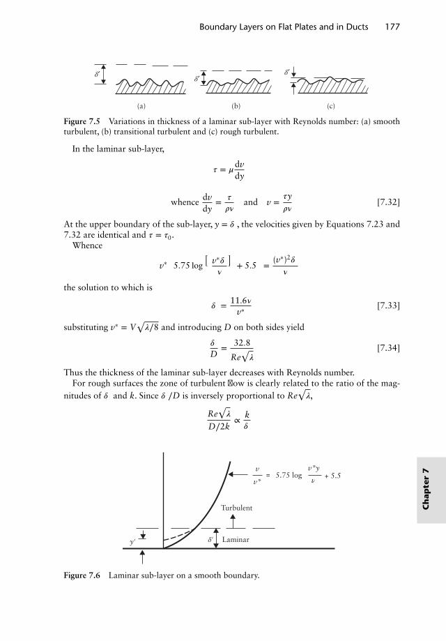
Boundary Layers on Flat Plates and in Ducts 177
)b()a(
δ′δ′ δ′
(c)
Figure 7.5 Variations in thickness of a laminar sub-layer with Reynolds number: (a) smoothturbulent, (b) transitional turbulent and (c) rough turbulent.
In the laminar sub-layer,
𝜏 = 𝜇dvdy
whence dvdy
= 𝜏
𝜌𝜈and v =
𝜏y𝜌𝜈
[7.32]
At the upper boundary of the sub-layer, y = 𝛿′, the velocities given by Equations 7.23 and7.32 are identical and 𝜏 = 𝜏0.
Whence
v∗[5.75 log
(v∗𝛿′
𝜈
)+ 5.5
]= (v∗)2𝛿′
𝜈
the solution to which is
𝛿′ = 11.6𝜈v∗
[7.33]
substituting v∗ = V√𝜆∕8 and introducing D on both sides yield
𝛿′
D= 32.8
Re√𝜆
[7.34]
Thus the thickness of the laminar sub-layer decreases with Reynolds number.For rough surfaces the zone of turbulent flow is clearly related to the ratio of the mag-
nitudes of 𝛿′ and k. Since 𝛿′∕D is inversely proportional to Re√𝜆,
Re√𝜆
D∕2k∝ k𝛿′
v
Turbulent
Laminar
+ 5.5= 5.75 log νv*
δ′y′
v*y
Figure 7.6 Laminar sub-layer on a smooth boundary.
Ch
apte
r7
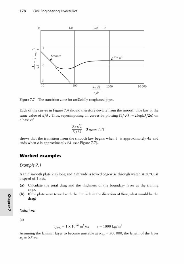
178 Civil Engineering Hydraulics
k/δ′0
1
1 2
3
10 100 1000 10 000
RoughSmooth
1.0
Re
2 lo
gr 0
r0/k
k
10
λ
λ
Figure 7.7 The transition zone for artificially roughened pipes.
Each of the curves in Figure 7.4 should therefore deviate from the smooth pipe law at thesame value of k∕𝛿′. Thus, superimposing all curves by plotting (1∕
√𝜆) − 2 log(D∕2k) on
a base of
Re√𝜆
D∕2k(Figure 7.7)
shows that the transition from the smooth law begins when 𝛿′ is approximately 4k andends when k is approximately 6𝛿′ (see Figure 7.7).
Worked examples
Example 7.1
A thin smooth plate 2 m long and 3 m wide is towed edgewise through water, at 20◦C, ata speed of 1 m/s.
(a) Calculate the total drag and the thickness of the boundary layer at the trailingedge.
(b) If the plate were towed with the 3 m side in the direction of flow, what would be thedrag?
Solution:
(a)
𝜈20◦C = 1 × 10⁻⁶ m2∕s; 𝜌 = 1000 kg∕m3
Assuming the laminar layer to become unstable at Rex = 500 000, the length of the layerx0 = 0.5 m.
Ch
apter
7
Boundary Layers on Flat Plates and in Ducts 179
Using Equation 7.11 for the combined drag in the laminar and turbulent layers,
Fs = 2
(1.33x0
Re1∕2x0
+ 0.074L
Re1∕5L
−0.074x0
Re1∕5x0
)B𝜌
U20
2
Fs = 2(
1.33 × 0.5707.1
+ 0.074 × 218.2
− 0.074 × 0.513.8
)3 × 1000 × 1
2Fs = 19.17 N
Boundary layer thickness: Experiments have shown that when the turbulent boundarylayer develops downstream of the laminar layer, the characteristics of the turbulent layerare those of one which develops at the leading edge. Thus,
𝛿L = 0.37L
Re1∕5L
= 0.041 m
If the drag were assumed to be entirely due to the turbulent boundary layer,
Fs = 2CfBL𝜌U2
0
2
Cf =0.074
Re1∕5L
= 0.07418.2
= 0.0041
Fs = 2 × 0.004 × 2 × 3 × 1000 × 12= 24.6 N
(b)
B = 2.0; L = 3.0
From Equation 7.11,
Fs = 2 × 2(
1.33 × 0.5707.1
+ 0.074 × 319.74
− 0.074 × 0.513.8
)1000 × 1
2= 19.01 N
Example 7.2
A 5 m long smooth model of a ship is towed in fresh water of kinematic viscosity 1 × 10⁻⁶
m2/s at 3.5 m/s. The wetted hull area is 1.4 m2. What is the skin friction drag?
Solution:
Assuming that a turbulent boundary layer develops at the leading edge,
drag = CfA𝜌U2
0
2
Cf =0.074
Re1∕5L
; ReL = 3.5 × 51 × 10−6
= 17.5 × 10⁶
whence Cf = 0.00263
Ch
apte
r7
180 Civil Engineering Hydraulics
and drag = 0.00263 × 1.4 × 1000 × 3.52
2= 22.55 N
Example 7.3
Water enters a 300 mm diameter test section of a water tunnel at a uniform velocity of15 m/s. Assuming that the boundary layer starts 0.5 m upstream of the test section, estimatethe increase in axial velocity at the end of a 3 m test section due to the growth of theboundary layer. Take 𝜈 = 1 × 10⁻⁶ m2/s.
Solution:
Length of boundary layer = 3.5 m
ReL = 15 × 3.5 × 106 = 52.5 × 10⁶
Re1∕5L = 35.0
𝛿L = 0.37L
Re1∕5L
= 0.37 × 3.535
= 0.037 m
From Section 7.5, assuming that the velocity distribution in the boundary layer is of theform
vU0
=(y𝛿
)1∕7(Equation 7.15)
the displacement thickness is expressed by
𝛿∗ = 𝛿
8(Equation 7.16)
or 𝛿∗ = 0.004625 m
Effective duct diameter = 300 − 9.25 = 290.75 mm
Then
U0A0 = ULAL
whence UL = 15(
300290.75
)2
= 15.97 m∕s
Change in pressure due to boundary layer formation: apply Bernoulli’s equation, assum-ing ideal fluid flow:
p0
𝜌g+
U20
2g=
pL
𝜌g+
U2L
2g
p0 − pL
𝜌g= Δh =
U2L − U2
0
2g
Δh = 15.972 − 152
2g= 1.53 m
Ch
apter
7
Boundary Layers on Flat Plates and in Ducts 181
Example 7.4
Water at 20◦C enters the 250 mm square working section of a water tunnel at 20 m/swith a turbulent boundary layer of thickness equal to that from a starting point 0.45 mupstream. Estimate the length of the sides of the divergent duct for constant pressure coreflow at 1, 2 and 3 m downstream from the duct entrance.
Solution:
From Equation 7.16, displacement thickness is
𝛿∗x =𝛿x
8
From Equation 7.7,
𝛿x = 0.37x
Re1∕5x
At 1 m from the entrance of the working section, the length of the boundary layer is1.45 m.
Rex = 20 × 1.451 × 10−6
= 29 × 106
whence 𝛿 = 0.01726 m
and 𝛿∗ = 0.00216 m = 2.16 mm
Thus the section size is 254.32 mm2.At 2 m from the entrance, the boundary layer is 2.45 m long.
𝛿∗ = 3.29 mm
⇒ section size = 256.58 mm
At 3 m from the entrance,
𝛿∗ = 4.32 m
⇒ section size = 258.64 mm
Example 7.5
The velocity distribution in the rough turbulent zone is expressed by
v√𝜏0∕𝜌
= 5.75 log( y
k
)+ 8.5 (Equation 7.27) (i)
Local axial velocities measured at 25 and 75 mm across a radius from the inner wall ofa 150 mm diameter pipe conveying water at 15◦C were 0.815 and 0.96 m/s, respectively.Calculate (a) the effective roughness size, (b) the hydraulic gradient and (c) the discharge.
Ch
apte
r7
182 Civil Engineering Hydraulics
Solution:
(a) Writing v∗ =√𝜏0∕𝜌 and inserting the pairs of values of v and y in the velocity distri-
bution equation,
0.96v∗
= 5.75 log(
75k
)+ 8.5 (ii)
0.815v∗
= 5.75 log(
25k
)+ 8.5 (iii)
Note: y can be expressed in millimetres since y∕k is dimensionless; the calculated value ofk will then be in millimetres. Hence,
0.96 − 0.815v∗
= 5.75 log(
7525
)
whence v∗ = 0.0528
and 𝜏0 = 2.79 N∕m2
Substituting for v∗ in (ii),
0.960.0528
= 5.75 log(
75k
)+ 8.5
whence k = 1.55 mm
(b) The hydraulic gradient (Sf = hf∕L) can be related to the boundary shear stress. Consideran element of flow in a pipeline (see Figure 7.8).
For steady, uniform flow, equate the forces on the element of length 𝛿L.
(p1 − p2)A + 𝜌gA𝛿L sin 𝛼 = 𝜏0P𝛿L
i.e.p1 − p2
𝜌g+ 𝛿z =
𝜏0P𝛿L
𝜌gA
or hf =𝜏0𝛿L𝜌gR
p1/ρg
V 2/2g hf
p2/ρg
δz
δL
τ0 α
Figure 7.8 Flow analysis in a pipeline.
Ch
apter
7
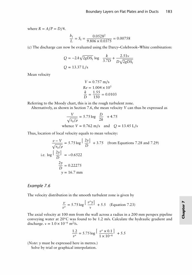
Boundary Layers on Flat Plates and in Ducts 183
where R = A∕P = D∕4.
hf
L= Sf =
0.05282
9.806 × 0.0375= 0.00758
(c) The discharge can now be evaluated using the Darcy–Colebrook–White combination:
Q = −2A√
2gDSf log
[k
3.7D+ 2.51𝜈
D√
2gDSf
]
Q = 13.37 L∕s
Mean velocity
V = 0.757 m∕s
Re = 1.004 × 10⁵
kD
= 1.55150
= 0.0103
Referring to the Moody chart, this is in the rough turbulent zone.Alternatively, as shown in Section 7.6, the mean velocity V can thus be expressed as
V√𝜏0∕𝜌
= 5.75 log( D
2k
)+ 4.75
whence V = 0.762 m∕s and Q = 13.45 L∕s
Thus, location of local velocity equals to mean velocity:
v − V√𝜏0∕𝜌
= 5.75 log(
2yD
)+ 3.75 (from Equations 7.28 and 7.29)
i.e. log(
2yD
)= −0.6522
2yD
= 0.22275
y = 16.7 mm
Example 7.6
The velocity distribution in the smooth turbulent zone is given by
vv∗
= 5.75 log(
v∗y𝜈
)+ 5.5 (Equation 7.23)
The axial velocity at 100 mm from the wall across a radius in a 200 mm perspex pipelineconveying water at 20◦C was found to be 1.2 m/s. Calculate the hydraulic gradient anddischarge. 𝜈 = 1.0 × 10⁻⁶ m2/s.
1.2v∗
= 5.75 log(
v∗ × 0.11 × 10⁻⁶
)+ 5.5
(Note: y must be expressed here in metres.)Solve by trial or graphical interpolation.
Ch
apte
r7
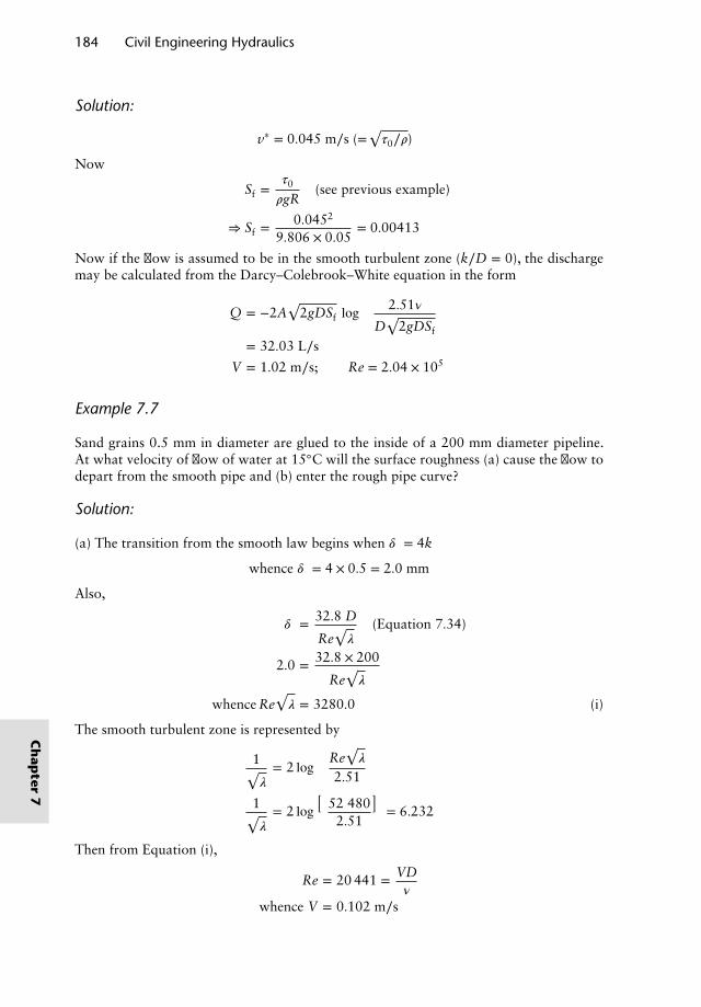
184 Civil Engineering Hydraulics
Solution:
v∗ = 0.045 m∕s (=√𝜏0∕𝜌)
Now
Sf =𝜏0
𝜌gR(see previous example)
⇒ Sf =0.0452
9.806 × 0.05= 0.00413
Now if the flow is assumed to be in the smooth turbulent zone (k∕D = 0), the dischargemay be calculated from the Darcy–Colebrook–White equation in the form
Q = −2A√
2gDSf log
(2.51𝜈
D√
2gDSf
)
= 32.03 L∕s
V = 1.02 m∕s; Re = 2.04 × 10⁵
Example 7.7
Sand grains 0.5 mm in diameter are glued to the inside of a 200 mm diameter pipeline.At what velocity of flow of water at 15◦C will the surface roughness (a) cause the flow todepart from the smooth pipe and (b) enter the rough pipe curve?
Solution:
(a) The transition from the smooth law begins when 𝛿′ = 4k
whence 𝛿′ = 4 × 0.5 = 2.0 mm
Also,
𝛿′ = 32.8 D
Re√𝜆
(Equation 7.34)
2.0 = 32.8 × 200
Re√𝜆
whence Re√𝜆 = 3280.0 (i)
The smooth turbulent zone is represented by
1√𝜆= 2 log
(Re
√𝜆
2.51
)
1√𝜆= 2 log
(52 480
2.51
)= 6.232
Then from Equation (i),
Re = 20 441 = VD𝜈
whence V = 0.102 m∕s
Ch
apter
7
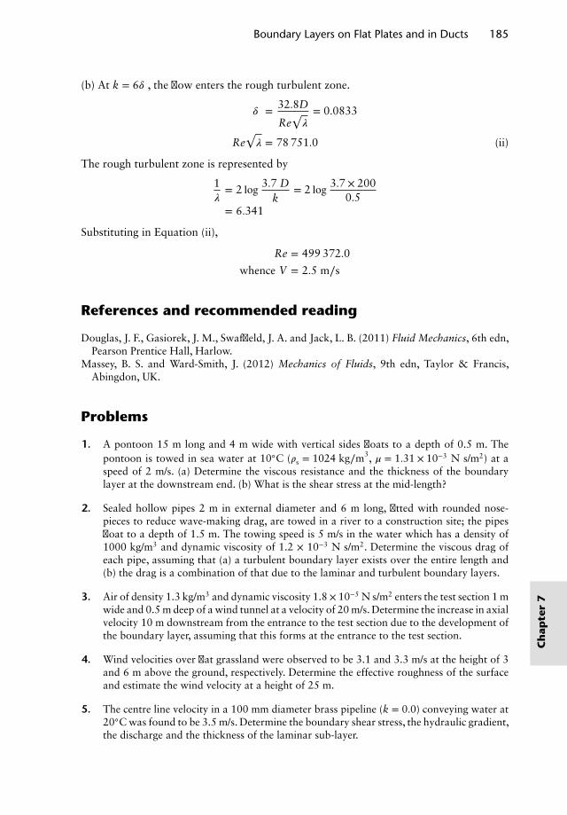
Boundary Layers on Flat Plates and in Ducts 185
(b) At k = 6𝛿′, the flow enters the rough turbulent zone.
𝛿′ = 32.8D
Re√𝜆
= 0.0833
Re√𝜆 = 78 751.0 (ii)
The rough turbulent zone is represented by
1𝜆= 2 log 3.7 D
k= 2 log 3.7 × 200
0.5= 6.341
Substituting in Equation (ii),
Re = 499 372.0
whence V = 2.5 m∕s
References and recommended reading
Douglas, J. F., Gasiorek, J. M., Swaffield, J. A. and Jack, L. B. (2011) Fluid Mechanics, 6th edn,Pearson Prentice Hall, Harlow.
Massey, B. S. and Ward-Smith, J. (2012) Mechanics of Fluids, 9th edn, Taylor & Francis,Abingdon, UK.
Problems
1. A pontoon 15 m long and 4 m wide with vertical sides floats to a depth of 0.5 m. Thepontoon is towed in sea water at 10◦C (𝜌s = 1024 kg∕m3, 𝜇 = 1.31 × 10⁻³ N s/m2) at aspeed of 2 m/s. (a) Determine the viscous resistance and the thickness of the boundarylayer at the downstream end. (b) What is the shear stress at the mid-length?
2. Sealed hollow pipes 2 m in external diameter and 6 m long, fitted with rounded nose-pieces to reduce wave-making drag, are towed in a river to a construction site; the pipesfloat to a depth of 1.5 m. The towing speed is 5 m/s in the water which has a density of1000 kg/m3 and dynamic viscosity of 1.2 × 10⁻³ N s/m2. Determine the viscous drag ofeach pipe, assuming that (a) a turbulent boundary layer exists over the entire length and(b) the drag is a combination of that due to the laminar and turbulent boundary layers.
3. Air of density 1.3 kg/m3 and dynamic viscosity 1.8 × 10⁻⁵ N s/m2 enters the test section 1 mwide and 0.5 m deep of a wind tunnel at a velocity of 20 m/s. Determine the increase in axialvelocity 10 m downstream from the entrance to the test section due to the development ofthe boundary layer, assuming that this forms at the entrance to the test section.
4. Wind velocities over flat grassland were observed to be 3.1 and 3.3 m/s at the height of 3and 6 m above the ground, respectively. Determine the effective roughness of the surfaceand estimate the wind velocity at a height of 25 m.
5. The centre line velocity in a 100 mm diameter brass pipeline (k = 0.0) conveying water at20◦C was found to be 3.5 m/s. Determine the boundary shear stress, the hydraulic gradient,the discharge and the thickness of the laminar sub-layer.
Ch
apte
r7
186 Civil Engineering Hydraulics
6. The velocities at 50 and 150 mm from the pipe wall of a 300 mm diameter pipeline convey-ing water at 15◦C were 1.423 and 1.674 m/s, respectively. Determine the effective rough-ness size, the hydraulic gradient, the discharge and the Darcy friction factor, and verify thatthe flow is in the rough turbulent zone.
7. Show that the equation
vmax − v√𝜏0∕𝜌
= 5.75 log D2y
applies to full-bore flow in circular pipes in both the rough and smooth turbulent zones.
Ch
apter
7
Chapter 8Steady Flow inOpen Channels
8.1 Introduction
Open channel flow, for example flow in rivers, canals and sewers not flowing full, is char-acterised by the presence of the interface between the liquid surface and the atmosphere.Therefore, unlike full pipe flow, where the pressure is normally above atmospheric pres-sure, but sometimes below it, the pressure on the surface of the liquid in open channel flowis always that of the ambient atmosphere.
The energy per unit weight of the liquid flowing in a channel at a section where thedepth of flow is y and the mean velocity is V is
H = z + y cos 𝜃 + 𝛼V2
2g(see Figure 8.1) [8.1]
where z is the position energy (or head), 𝜃 the bed slope and 𝛼 the Coriolis coefficient (seealso Equation 3.11).
𝛼 = 1AV3 ∫
A
0v3 dA
The motivating force establishing flow is predominantly the gravity force componentacting in parallel with the bed slope, but net pressure forces and inertia forces may also bepresent. Flow in channels may be unsteady, resulting from changes in inflow such as floodsor changes in depth caused by control gate operation. Steady flow can either be uniform orbe varied depending upon whether or not the mean velocity is constant with distance. Ingradually varied flow there is a gentle change in depth with distance; a common example isthe backwater curve (Figure 8.2a). Rapidly varied surface profiles are created by changesin channel geometry, for example flow through a venturi flume (Figure 8.2b).
Steady, uniform flow occurs when the motivating forces and drag forces are exactlybalanced over the reach under consideration. This type of flow is analogous with steadypressurised flow in a pipeline of constant diameter. Thus the area of flow in the channel
Nalluri & Featherstone’s Civil Engineering Hydraulics: Essential Theory with Worked Examples,Sixth Edition. Martin Marriott.© 2016 John Wiley & Sons, Ltd. Published 2016 by John Wiley & Sons, Ltd.Companion Website: www.wiley.com/go/Marriott
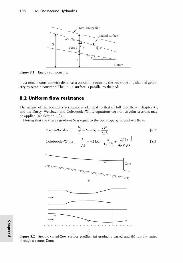
188 Civil Engineering Hydraulics
Total energy line
Liquid surface
Datum
y cos θ
αV2/2g
z
yH
θ
Figure 8.1 Energy components.
must remain constant with distance, a condition requiring the bed slope and channel geom-etry to remain constant. The liquid surface is parallel to the bed.
8.2 Uniform flow resistance
The nature of the boundary resistance is identical to that of full pipe flow (Chapter 4),and the Darcy–Weisbach and Colebrook–White equations for non-circular sections maybe applied (see Section 4.2).
Noting that the energy gradient Sf is equal to the bed slope S0 in uniform flow:
Darcy–Weisbach:hf
L= Sf = S0 = 𝜆V2
8gR[8.2]
Colebrook–White: l√𝜆= −2 log
(k
14.8R+ 2.51𝜈
4RV√𝜆
)[8.3]
(a)
(b)
Gate
Figure 8.2 Steady, varied-flow surface profiles: (a) gradually varied and (b) rapidly variedthrough a venturi flume
Ch
apter
8
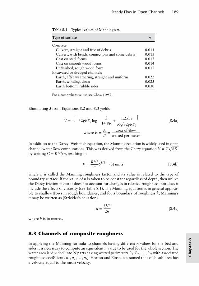
Steady Flow in Open Channels 189
Table 8.1 Typical values of Manning’s n.
Type of surface n
ConcreteCulvert, straight and free of debris 0.011Culvert, with bends, connections and some debris 0.013Cast on steel forms 0.013Cast on smooth wood forms 0.014Unfinished, rough wood form 0.017
Excavated or dredged channelsEarth, after weathering, straight and uniform 0.022Earth, winding, clean 0.025Earth bottom, rubble sides 0.030
For a comprehensive list, see Chow (1959).
Eliminating 𝜆 from Equations 8.2 and 8.3 yields
V = −√
32gRS0 log
(k
14.8R+ 1.255𝜈
R√
32gRS0
)[8.4a]
where R = AP
= area of flowwetted perimeter
In addition to the Darcy–Weisbach equation, the Manning equation is widely used in openchannel water flow computations. This was derived from the Chezy equation V = C
√RS0
by writing C = R1∕6∕n, resulting in
V = R2∕3
nS1∕2
0 (SI units) [8.4b]
where n is called the Manning roughness factor and its value is related to the type ofboundary surface. If the value of n is taken to be constant regardless of depth, then unlikethe Darcy friction factor it does not account for changes in relative roughness; nor does itinclude the effects of viscosity (see Table 8.1). The Manning equation is in general applica-ble to shallow flows in rough boundaries, and for a boundary of roughness k, Manning’sn may be written as (Strickler’s equation)
n = k1∕6
26[8.4c]
where k is in metres.
8.3 Channels of composite roughness
In applying the Manning formula to channels having different n values for the bed andsides it is necessary to compute an equivalent n value to be used for the whole section. Thewater area is ‘divided’ into N parts having wetted perimeters P1, P2,… , PN with associatedroughness coefficients n1, n2,… , nN. Horton and Einstein assumed that each sub-area hasa velocity equal to the mean velocity.
Ch
apte
r8
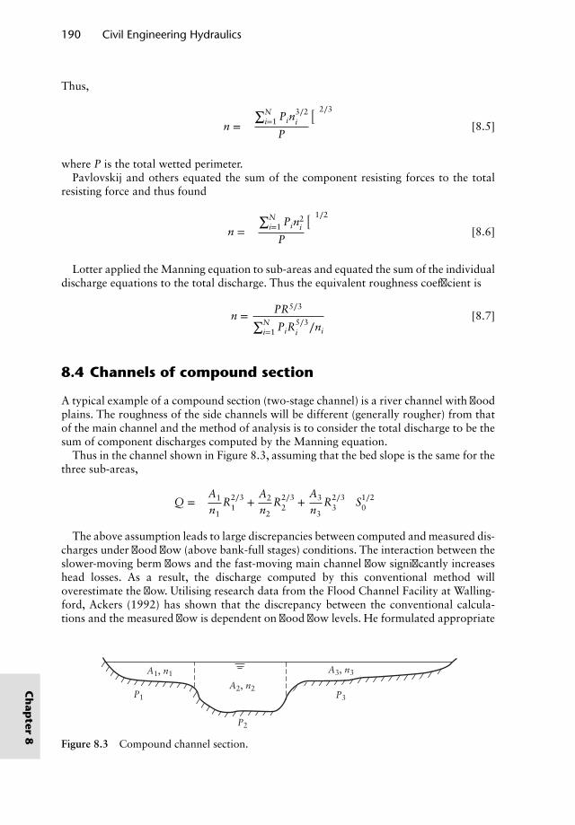
190 Civil Engineering Hydraulics
Thus,
n =
(∑Ni=1 Pin
3∕2i
P
)2∕3
[8.5]
where P is the total wetted perimeter.Pavlovskij and others equated the sum of the component resisting forces to the total
resisting force and thus found
n =
(∑Ni=1 Pin
2i
P
)1∕2
[8.6]
Lotter applied the Manning equation to sub-areas and equated the sum of the individualdischarge equations to the total discharge. Thus the equivalent roughness coefficient is
n = PR5∕3∑Ni=1 PiR
5∕3i ∕ni
[8.7]
8.4 Channels of compound section
A typical example of a compound section (two-stage channel) is a river channel with floodplains. The roughness of the side channels will be different (generally rougher) from thatof the main channel and the method of analysis is to consider the total discharge to be thesum of component discharges computed by the Manning equation.
Thus in the channel shown in Figure 8.3, assuming that the bed slope is the same for thethree sub-areas,
Q =(
A1
n1R2∕3
1 +A2
n2R2∕3
2 +A3
n3R2∕3
3
)S1∕2
0
The above assumption leads to large discrepancies between computed and measured dis-charges under flood flow (above bank-full stages) conditions. The interaction between theslower-moving berm flows and the fast-moving main channel flow significantly increaseshead losses. As a result, the discharge computed by this conventional method willoverestimate the flow. Utilising research data from the Flood Channel Facility at Walling-ford, Ackers (1992) has shown that the discrepancy between the conventional calcula-tions and the measured flow is dependent on flood flow levels. He formulated appropriate
A1, n1
A2, n2
A3, n3
P3
P2
P1
Figure 8.3 Compound channel section.
Ch
apter
8
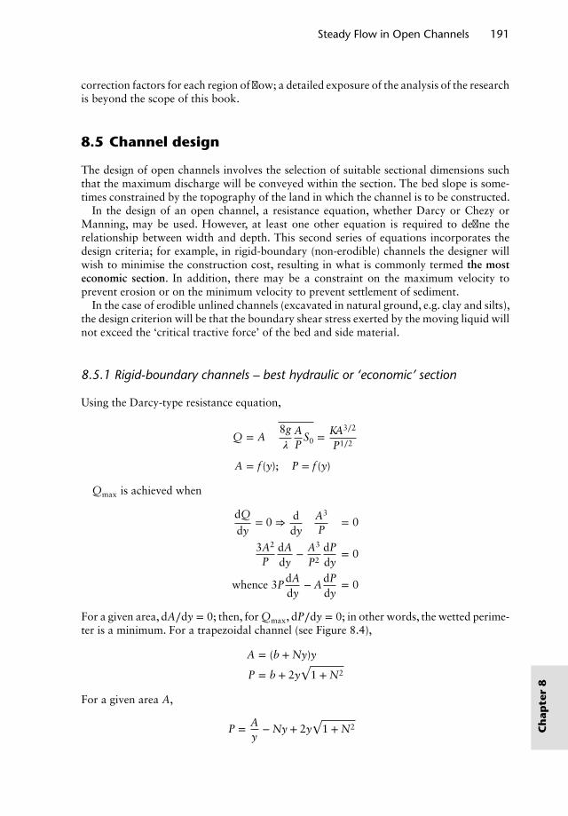
Steady Flow in Open Channels 191
correction factors for each region of flow; a detailed exposure of the analysis of the researchis beyond the scope of this book.
8.5 Channel design
The design of open channels involves the selection of suitable sectional dimensions suchthat the maximum discharge will be conveyed within the section. The bed slope is some-times constrained by the topography of the land in which the channel is to be constructed.
In the design of an open channel, a resistance equation, whether Darcy or Chezy orManning, may be used. However, at least one other equation is required to define therelationship between width and depth. This second series of equations incorporates thedesign criteria; for example, in rigid-boundary (non-erodible) channels the designer willwish to minimise the construction cost, resulting in what is commonly termed the mosteconomic section. In addition, there may be a constraint on the maximum velocity toprevent erosion or on the minimum velocity to prevent settlement of sediment.
In the case of erodible unlined channels (excavated in natural ground, e.g. clay and silts),the design criterion will be that the boundary shear stress exerted by the moving liquid willnot exceed the ‘critical tractive force’ of the bed and side material.
8.5.1 Rigid-boundary channels – best hydraulic or ‘economic’ section
Using the Darcy-type resistance equation,
Q = A
√8g𝜆
AP
S0 = KA3∕2
P1∕2
A = f (y); P = f (y)
Qmax is achieved when
dQ
dy= 0 ⇒
ddy
(A3
P
)= 0
3A2
PdAdy
− A3
P2
dPdy
= 0
whence 3PdAdy
− AdPdy
= 0
For a given area, dA∕dy = 0; then, for Qmax, dP∕dy = 0; in other words, the wetted perime-ter is a minimum. For a trapezoidal channel (see Figure 8.4),
A = (b + Ny)y
P = b + 2y√
1 + N2
For a given area A,
P = Ay− Ny + 2y
√1 + N2 C
hap
ter
8
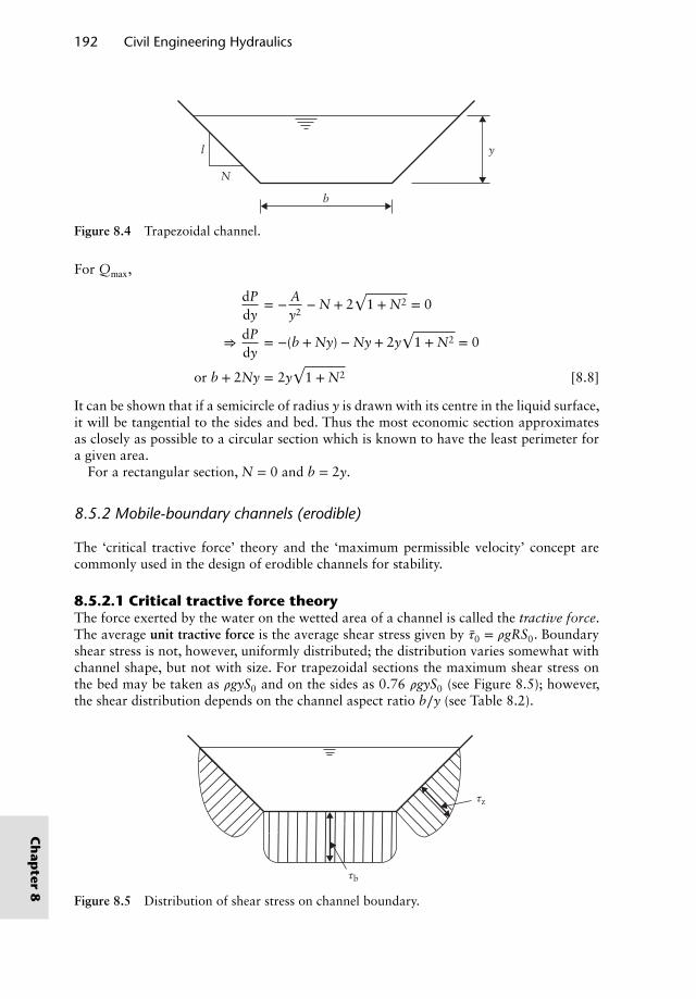
192 Civil Engineering Hydraulics
N
y
b
l
Figure 8.4 Trapezoidal channel.
For Qmax,
dPdy
= − Ay2
− N + 2√
1 + N2 = 0
⇒dPdy
= −(b + Ny) − Ny + 2y√
1 + N2 = 0
or b + 2Ny = 2y√
1 + N2 [8.8]
It can be shown that if a semicircle of radius y is drawn with its centre in the liquid surface,it will be tangential to the sides and bed. Thus the most economic section approximatesas closely as possible to a circular section which is known to have the least perimeter fora given area.
For a rectangular section, N = 0 and b = 2y.
8.5.2 Mobile-boundary channels (erodible)
The ‘critical tractive force’ theory and the ‘maximum permissible velocity’ concept arecommonly used in the design of erodible channels for stability.
8.5.2.1 Critical tractive force theoryThe force exerted by the water on the wetted area of a channel is called the tractive force.The average unit tractive force is the average shear stress given by 𝜏0 = 𝜌gRS0. Boundaryshear stress is not, however, uniformly distributed; the distribution varies somewhat withchannel shape, but not with size. For trapezoidal sections the maximum shear stress onthe bed may be taken as 𝜌gyS0 and on the sides as 0.76 𝜌gyS0 (see Figure 8.5); however,the shear distribution depends on the channel aspect ratio b∕y (see Table 8.2).
τz
τb
Figure 8.5 Distribution of shear stress on channel boundary.
Ch
apter
8
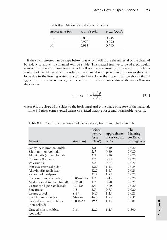
Steady Flow in Open Channels 193
Table 8.2 Maximum bed/side shear stress.
Aspect ratio b∕y 𝝉b 𝐦𝐚𝐱∕𝝆gyS0 𝝉s 𝐦𝐚𝐱∕𝝆gyS0
2 0.890 0.7354 0.970 0.750
>8 0.985 0.780
If the shear stresses can be kept below that which will cause the material of the channelboundary to move, the channel will be stable. The critical tractive force of a particularmaterial is the unit tractive force, which will not cause erosion of the material on a hori-zontal surface. Material on the sides of the channel is subjected, in addition to the shearforce due to the flowing water, to a gravity force down the slope. It can be shown that if𝜏cb is the critical tractive force, the maximum critical shear stress due to the water flow onthe sides is
𝜏cs = 𝜏cb
√1 − sin2
𝜃
sin2𝜙
[8.9]
where 𝜃 is the slope of the sides to the horizontal and 𝜙 the angle of repose of the material.Table 8.3 gives some typical values of critical tractive force and permissible velocity.
Table 8.3 Critical tractive force and mean velocity for different bed materials.
Critical Thetractive Approximate Manningforce mean velocity coefficient
Material Size (mm) (N/m2) (m/s) of roughness
Sandy loam (non-colloidal) 2.0 0.50 0.020Silt loam (non-colloidal) 2.5 0.60 0.020Alluvial silt (non-colloidal) 2.5 0.60 0.020Ordinary firm loam 3.7 0.75 0.020Volcanic ash 3.7 0.75 0.020Stiff clay (very colloidal) 1.22 1.15 0.025Alluvial silts (colloidal) 12.2 1.15 0.025Shales and hardpans 31.8 1.85 0.025Fine sand (non-colloidal) 0.062–0.25 1.2 0.45 0.020Medium sand (non-colloidal) 0.25–0.5 1.7 0.50 0.020Coarse sand (non-colloidal) 0.5–2.0 2.5 0.60 0.020Fine gravel 4–8 3.7 0.75 0.020Coarse gravel 8–64 14.7 1.25 0.025Cobbles and shingles 64–256 44.0 1.55 0.035Graded loam and cobbles(non-colloidal)
0.004–64 19.6 1.15 0.300
Graded silts to cobbles(colloidal)
0–64 22.0 1.25 0.300
Ch
apte
r8
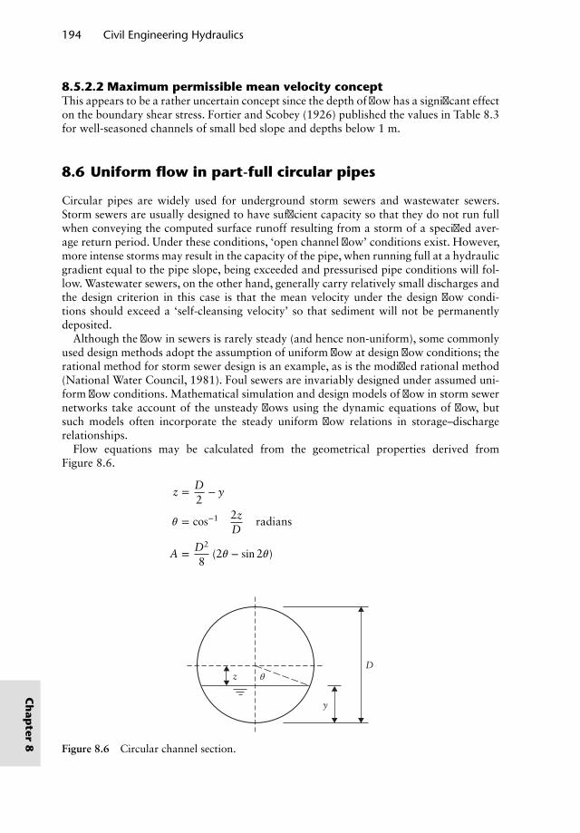
194 Civil Engineering Hydraulics
8.5.2.2 Maximum permissible mean velocity conceptThis appears to be a rather uncertain concept since the depth of flow has a significant effecton the boundary shear stress. Fortier and Scobey (1926) published the values in Table 8.3for well-seasoned channels of small bed slope and depths below 1 m.
8.6 Uniform flow in part-full circular pipes
Circular pipes are widely used for underground storm sewers and wastewater sewers.Storm sewers are usually designed to have sufficient capacity so that they do not run fullwhen conveying the computed surface runoff resulting from a storm of a specified aver-age return period. Under these conditions, ‘open channel flow’ conditions exist. However,more intense storms may result in the capacity of the pipe, when running full at a hydraulicgradient equal to the pipe slope, being exceeded and pressurised pipe conditions will fol-low. Wastewater sewers, on the other hand, generally carry relatively small discharges andthe design criterion in this case is that the mean velocity under the design flow condi-tions should exceed a ‘self-cleansing velocity’ so that sediment will not be permanentlydeposited.
Although the flow in sewers is rarely steady (and hence non-uniform), some commonlyused design methods adopt the assumption of uniform flow at design flow conditions; therational method for storm sewer design is an example, as is the modified rational method(National Water Council, 1981). Foul sewers are invariably designed under assumed uni-form flow conditions. Mathematical simulation and design models of flow in storm sewernetworks take account of the unsteady flows using the dynamic equations of flow, butsuch models often incorporate the steady uniform flow relations in storage–dischargerelationships.
Flow equations may be calculated from the geometrical properties derived fromFigure 8.6.
z = D2
− y
𝜃 = cos−1(
2zD
)radians
A = D2
8(2𝜃 − sin2𝜃)
D
y
z θ
Figure 8.6 Circular channel section.
Ch
apter
8
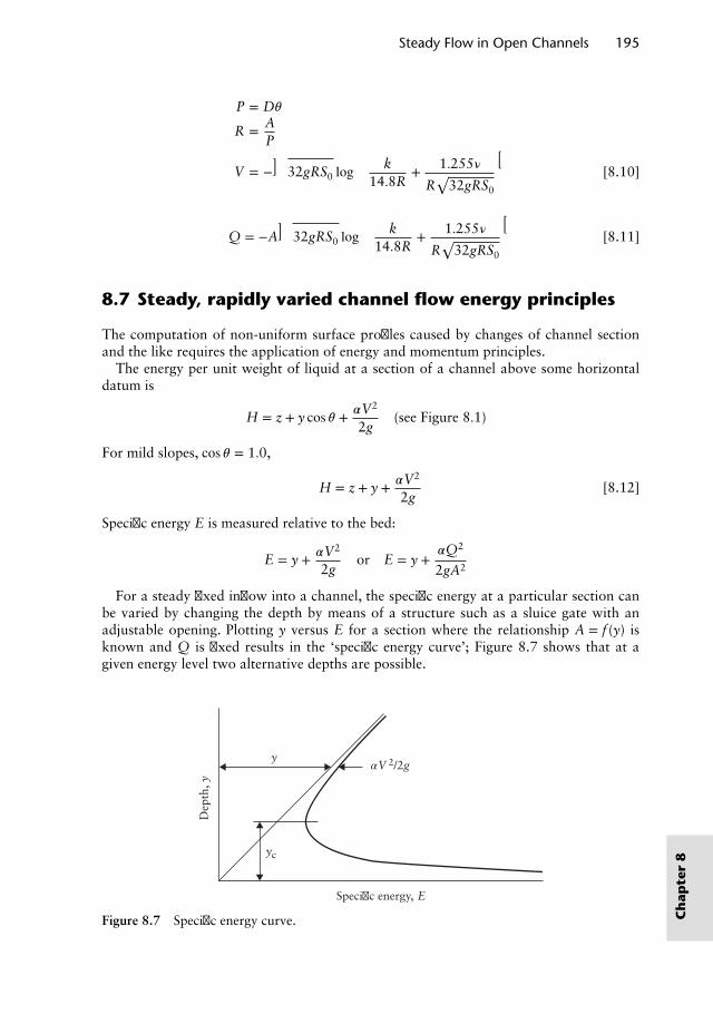
Steady Flow in Open Channels 195
P = D𝜃
R = AP
V = −√
32gRS0 log
(k
14.8R+ 1.255𝜈
R√
32gRS0
)[8.10]
Q = −A√
32gRS0 log
(k
14.8R+ 1.255𝜈
R√
32gRS0
)[8.11]
8.7 Steady, rapidly varied channel flow energy principles
The computation of non-uniform surface profiles caused by changes of channel sectionand the like requires the application of energy and momentum principles.
The energy per unit weight of liquid at a section of a channel above some horizontaldatum is
H = z + y cos 𝜃 + 𝛼V2
2g(see Figure 8.1)
For mild slopes, cos 𝜃 = 1.0,
H = z + y + 𝛼V2
2g[8.12]
Specific energy E is measured relative to the bed:
E = y + 𝛼V2
2gor E = y +
𝛼Q2
2gA2
For a steady fixed inflow into a channel, the specific energy at a particular section canbe varied by changing the depth by means of a structure such as a sluice gate with anadjustable opening. Plotting y versus E for a section where the relationship A = f (y) isknown and Q is fixed results in the ‘specific energy curve’; Figure 8.7 shows that at agiven energy level two alternative depths are possible.
y
yc
Specific energy, E
αV 2/2g
Dep
th, y
Figure 8.7 Specific energy curve. Ch
apte
r8
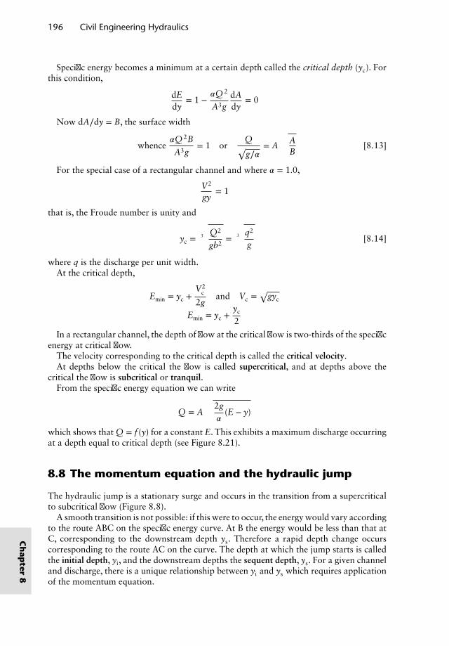
196 Civil Engineering Hydraulics
Specific energy becomes a minimum at a certain depth called the critical depth (yc). Forthis condition,
dEdy
= 1 −𝛼Q 2
A3gdAdy
= 0
Now dA∕dy = B, the surface width
whence𝛼Q 2B
A3g= 1 or
Q√g∕𝛼
= A
√AB
[8.13]
For the special case of a rectangular channel and where 𝛼 = 1.0,
V2
gy= 1
that is, the Froude number is unity and
yc =3
√Q2
gb2= 3
√q2
g[8.14]
where q is the discharge per unit width.At the critical depth,
Emin = yc +V2
c
2gand Vc =
√gyc
Emin = yc +yc
2
In a rectangular channel, the depth of flow at the critical flow is two-thirds of the specificenergy at critical flow.
The velocity corresponding to the critical depth is called the critical velocity.At depths below the critical the flow is called supercritical, and at depths above the
critical the flow is subcritical or tranquil.From the specific energy equation we can write
Q = A
√2g𝛼
(E − y)
which shows that Q = f (y) for a constant E. This exhibits a maximum discharge occurringat a depth equal to critical depth (see Figure 8.21).
8.8 The momentum equation and the hydraulic jump
The hydraulic jump is a stationary surge and occurs in the transition from a supercriticalto subcritical flow (Figure 8.8).
A smooth transition is not possible: if this were to occur, the energy would vary accordingto the route ABC on the specific energy curve. At B the energy would be less than that atC, corresponding to the downstream depth ys. Therefore a rapid depth change occurscorresponding to the route AC on the curve. The depth at which the jump starts is calledthe initial depth, yi, and the downstream depths the sequent depth, ys. For a given channeland discharge, there is a unique relationship between yi and ys which requires applicationof the momentum equation.
Ch
apter
8
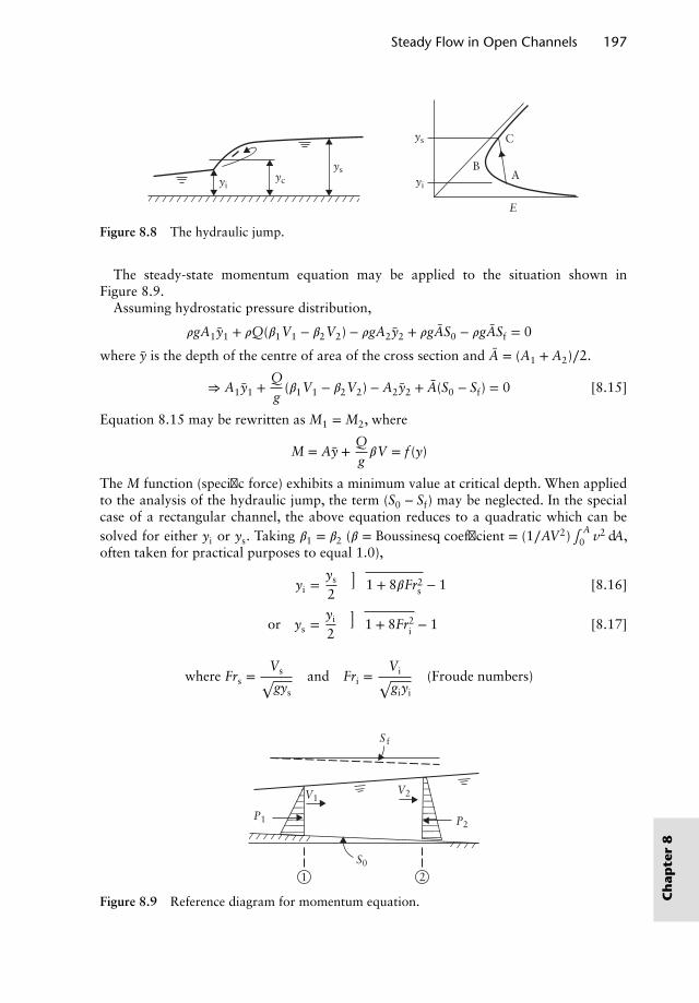
Steady Flow in Open Channels 197
E
yiyiyc
ys
ys
B
C
A
Figure 8.8 The hydraulic jump.
The steady-state momentum equation may be applied to the situation shown inFigure 8.9.
Assuming hydrostatic pressure distribution,
𝜌gA1y1 + 𝜌Q(𝛽1V1 − 𝛽2V2) − 𝜌gA2y2 + 𝜌gAS0 − 𝜌gASf = 0
where y is the depth of the centre of area of the cross section and A = (A1 + A2)∕2.
⇒ A1y1 +Qg
(𝛽1V1 − 𝛽2V2) − A2y2 + A(S0 − Sf) = 0 [8.15]
Equation 8.15 may be rewritten as M1 = M2, where
M = Ay +Qg𝛽V = f (y)
The M function (specific force) exhibits a minimum value at critical depth. When appliedto the analysis of the hydraulic jump, the term (S0 − Sf) may be neglected. In the specialcase of a rectangular channel, the above equation reduces to a quadratic which can besolved for either yi or ys. Taking 𝛽1 = 𝛽2 (𝛽 = Boussinesq coefficient = (1∕AV2) ∫ A
0 v2 dA,often taken for practical purposes to equal 1.0),
yi =ys
2
(√1 + 8𝛽Fr2
s − 1)
[8.16]
or ys =yi
2
(√1 + 8Fr2
i − 1)
[8.17]
where Frs =Vs√gys
and Fri =Vi√giyi
(Froude numbers)
V2V1
P1 P2
S0
21
S f
Figure 8.9 Reference diagram for momentum equation. Ch
apte
r8
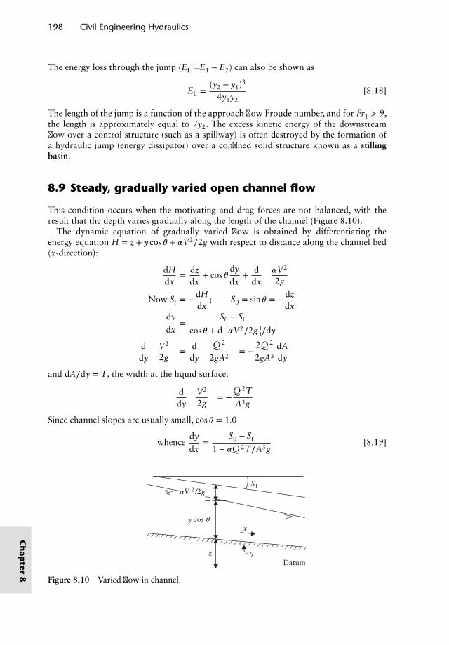
198 Civil Engineering Hydraulics
The energy loss through the jump (EL =E1 − E2) can also be shown as
EL =(y2 − y1)3
4y1y2[8.18]
The length of the jump is a function of the approach flow Froude number, and for Fr1 > 9,the length is approximately equal to 7y2. The excess kinetic energy of the downstreamflow over a control structure (such as a spillway) is often destroyed by the formation ofa hydraulic jump (energy dissipator) over a confined solid structure known as a stillingbasin.
8.9 Steady, gradually varied open channel flow
This condition occurs when the motivating and drag forces are not balanced, with theresult that the depth varies gradually along the length of the channel (Figure 8.10).
The dynamic equation of gradually varied flow is obtained by differentiating theenergy equation H = z + y cos 𝜃 + 𝛼V2∕2g with respect to distance along the channel bed(x-direction):
dHdx
= dzdx
+ cos 𝜃dy
dx+ d
dx
(𝛼V2
2g
)
Now Sf = −dHdx
; S0 = sin 𝜃 = − dzdx
dy
dx=
S0 − Sf
cos 𝜃 + d(𝛼V2∕2g
)∕dy
ddy
(V2
2g
)= d
dy
(Q 2
2gA2
)= −
2Q 2
2gA3
dAdy
and dA∕dy = T, the width at the liquid surface.
ddy
(V2
2g
)= −
Q2T
A3g
Since channel slopes are usually small, cos 𝜃 = 1.0
whencedy
dx=
S0 − Sf
1 − 𝛼Q 2T∕A3g[8.19]
αV 2 /2g
y cos θ
θDatum
S f
z
x
Figure 8.10 Varied flow in channel.
Ch
apter
8
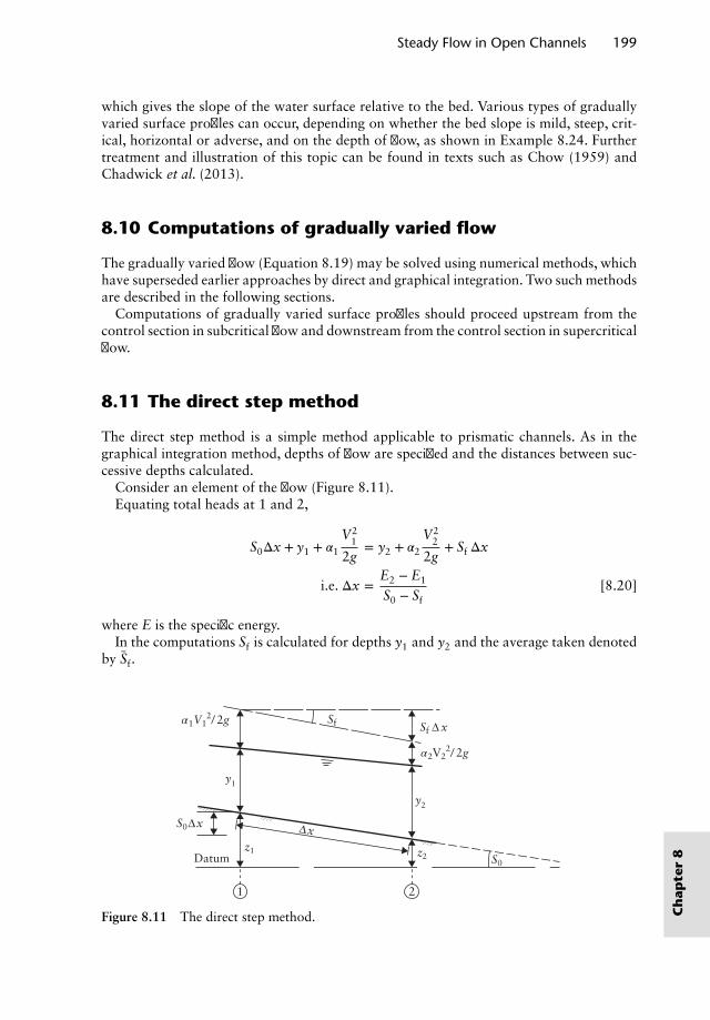
Steady Flow in Open Channels 199
which gives the slope of the water surface relative to the bed. Various types of graduallyvaried surface profiles can occur, depending on whether the bed slope is mild, steep, crit-ical, horizontal or adverse, and on the depth of flow, as shown in Example 8.24. Furthertreatment and illustration of this topic can be found in texts such as Chow (1959) andChadwick et al. (2013).
8.10 Computations of gradually varied flow
The gradually varied flow (Equation 8.19) may be solved using numerical methods, whichhave superseded earlier approaches by direct and graphical integration. Two such methodsare described in the following sections.
Computations of gradually varied surface profiles should proceed upstream from thecontrol section in subcritical flow and downstream from the control section in supercriticalflow.
8.11 The direct step method
The direct step method is a simple method applicable to prismatic channels. As in thegraphical integration method, depths of flow are specified and the distances between suc-cessive depths calculated.
Consider an element of the flow (Figure 8.11).Equating total heads at 1 and 2,
S0Δx + y1 + 𝛼1
V21
2g= y2 + 𝛼2
V22
2g+ Sf Δx
i.e. Δx =E2 − E1
S0 − Sf[8.20]
where E is the specific energy.In the computations Sf is calculated for depths y1 and y2 and the average taken denoted
by Sf.
y1
z1 z2
y2
Sfα1V12/ 2g
α2V22/ 2g
S0Δx
S0
Δx
Sf Δ x
Datum
21
Figure 8.11 The direct step method. Ch
apte
r8
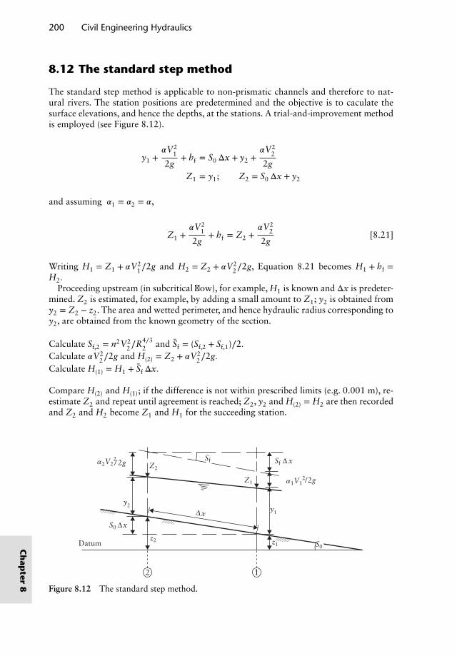
200 Civil Engineering Hydraulics
8.12 The standard step method
The standard step method is applicable to non-prismatic channels and therefore to nat-ural rivers. The station positions are predetermined and the objective is to caculate thesurface elevations, and hence the depths, at the stations. A trial-and-improvement methodis employed (see Figure 8.12).
y1 +𝛼V2
1
2g+ hf = S0 Δx + y2 +
𝛼V22
2gZ1 = y1; Z2 = S0 Δx + y2
and assuming 𝛼1 = 𝛼2 = 𝛼,
Z1 +𝛼V2
1
2g+ hf = Z2 +
𝛼V22
2g[8.21]
Writing H1 = Z1 + 𝛼V21∕2g and H2 = Z2 + 𝛼V2
2∕2g, Equation 8.21 becomes H1 + hf =H2.
Proceeding upstream (in subcritical flow), for example, H1 is known and Δx is predeter-mined. Z2 is estimated, for example, by adding a small amount to Z1; y2 is obtained fromy2 = Z2 − z2. The area and wetted perimeter, and hence hydraulic radius corresponding toy2, are obtained from the known geometry of the section.
Calculate Sf,2 = n2V22∕R4∕3
2 and Sf = (Sf,2 + Sf,1)∕2.Calculate 𝛼V2
2∕2g and H(2) = Z2 + 𝛼V22∕2g.
Calculate H(1) = H1 + Sf Δx.
Compare H(2) and H(1); if the difference is not within prescribed limits (e.g. 0.001 m), re-estimate Z2 and repeat until agreement is reached; Z2, y2 and H(2) = H2 are then recordedand Z2 and H2 become Z1 and H1 for the succeeding station.
y2
z1z2
Z2
Z1
y1
Sfα2V22
α1V12
S0 Δx
Δx
Sf Δ x
Datum
12
/ 2g
/2g
S0
Figure 8.12 The standard step method.
Ch
apter
8
Steady Flow in Open Channels 201
8.13 Canal delivery problems
When a channel is connected to two reservoirs its discharge capacity depends upon inlet(upstream) and outlet (downstream) conditions imposed by the water levels in the reser-voirs. The reservoir–canal–reservoir interaction depends upon the channel characteristicssuch as its boundary roughness, its slope, the length between reservoirs and the state ofwater levels in the reservoirs.
8.13.1 Case 1: Upstream reservoir water level is constant
For a given boundary characteristic the discharge rate in the channel depends on whether itis a long or short channel with a mild or critical or steep bed slope. A long channel deliverswater with no interference from the downstream water levels (i.e. with no downstreamcontrol); only the inlet controls the flow rate. This suggests that any water surface profileslikely to develop with the available downstream water levels will not be long enough toreach the inlet, thus allowing the inlet to discharge freely. On the other hand, if the channelis short, the water surface profiles could submerge the inlet and this submergence affectsthe flow rate. The types of profile and their appropriate lengths would depend on thechannel slope.
(a) Long channel with mild slope (see Figure 8.20): The flow on entering the inlet estab-lishes uniform conditions from a short distance downstream of the entry. Thus atentry we have two simultaneous equations to compute the flow depth y0 and dis-charge Q0 or velocity:
Energy equation: upstream water level above inlet,H = y0 + 𝛼V2∕2g + K𝛼V2∕2g
Uniform flow resistance equation (say Manning’s), V = (1∕n)R2∕3S1∕2
See Example 8.7 for the solution of these two equations.(b) Long channel with critical slope: The flow now establishes with its normal flow
depth equal to the critical depth from the inlet, thus allowing maximum possibledischarge through the channel. We now have at the channel entry two equationsenabling the computations of Q and y:
Energy equation at inlet: H = yc + 𝛼V2c ∕2g + 𝛼KV2
c ∕2g
Either the critical depth criterion 𝛼Q2B∕gA2 = 1 or the appropriate uniform flowresistance equation.
(c) Long channel with steep slope: The flow depth at the entry is critical, the channeldelivering maximum possible discharge, and if the channel is sufficiently long uniformflow will establish further downstream of the entry. The flow up to this point will benon-uniform with the development of an S2 profile which asymptotically merges withthe uniform flow depth (see Example 8.8).
The problems are much more complicated if the channels are short; in other words, anydownstream control or disturbance (e.g. downstream water level variations) extends itsinfluence right up to the entry, thus submerging the entry and changing the delivery capac-ities of the channel. Such problems are solved iteratively by computer. C
hap
ter
8
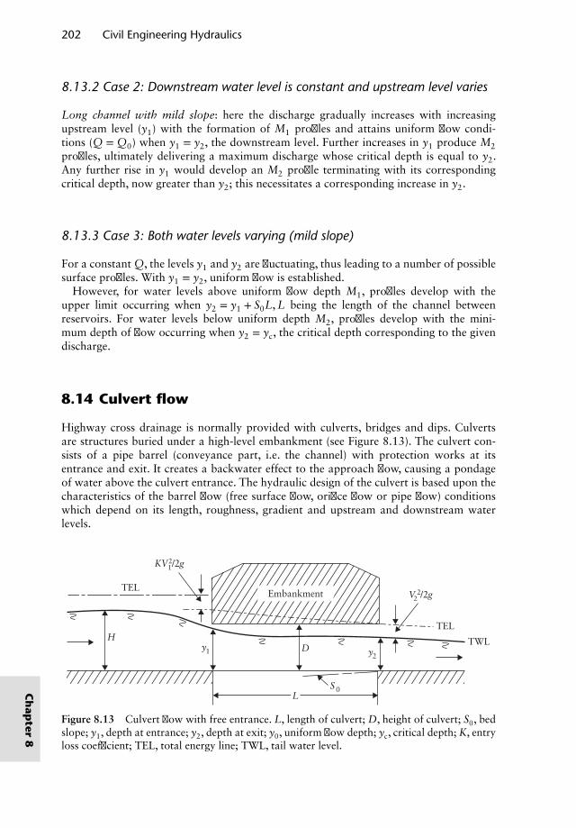
202 Civil Engineering Hydraulics
8.13.2 Case 2: Downstream water level is constant and upstream level varies
Long channel with mild slope: here the discharge gradually increases with increasingupstream level (y1) with the formation of M1 profiles and attains uniform flow condi-tions (Q = Q0) when y1 = y2, the downstream level. Further increases in y1 produce M2profiles, ultimately delivering a maximum discharge whose critical depth is equal to y2.Any further rise in y1 would develop an M2 profile terminating with its correspondingcritical depth, now greater than y2; this necessitates a corresponding increase in y2.
8.13.3 Case 3: Both water levels varying (mild slope)
For a constant Q, the levels y1 and y2 are fluctuating, thus leading to a number of possiblesurface profiles. With y1 = y2, uniform flow is established.
However, for water levels above uniform flow depth M1, profiles develop with theupper limit occurring when y2 = y1 + S0L, L being the length of the channel betweenreservoirs. For water levels below uniform depth M2, profiles develop with the mini-mum depth of flow occurring when y2 = yc, the critical depth corresponding to the givendischarge.
8.14 Culvert flow
Highway cross drainage is normally provided with culverts, bridges and dips. Culvertsare structures buried under a high-level embankment (see Figure 8.13). The culvert con-sists of a pipe barrel (conveyance part, i.e. the channel) with protection works at itsentrance and exit. It creates a backwater effect to the approach flow, causing a pondageof water above the culvert entrance. The hydraulic design of the culvert is based upon thecharacteristics of the barrel flow (free surface flow, orifice flow or pipe flow) conditionswhich depend on its length, roughness, gradient and upstream and downstream waterlevels.
TEL
KV12/2g
V22/2g
y1
S0
y2
HTEL
TWLD
Embankment
L
Figure 8.13 Culvert flow with free entrance. L, length of culvert; D, height of culvert; S0, bedslope; y1, depth at entrance; y2, depth at exit; y0, uniform flow depth; yc, critical depth; K, entryloss coefficient; TEL, total energy line; TWL, tail water level.
Ch
apter
8
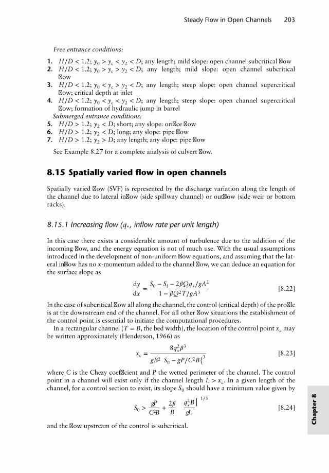
Steady Flow in Open Channels 203
Free entrance conditions:
1. H∕D < 1.2; y0 > yc < y2 < D; any length; mild slope: open channel subcritical flow2. H∕D < 1.2; y0 > yc > y2 < D; any length; mild slope: open channel subcritical
flow3. H∕D < 1.2; y0 < yc > y2 < D; any length; steep slope: open channel supercritical
flow; critical depth at inlet4. H∕D < 1.2; y0 < yc < y2 < D; any length; steep slope: open channel supercritical
flow; formation of hydraulic jump in barrelSubmerged entrance conditions:
5. H∕D > 1.2; y2 < D; short; any slope: orifice flow6. H∕D > 1.2; y2 < D; long; any slope: pipe flow7. H∕D > 1.2; y2 > D; any length; any slope: pipe flow
See Example 8.27 for a complete analysis of culvert flow.
8.15 Spatially varied flow in open channels
Spatially varied flow (SVF) is represented by the discharge variation along the length ofthe channel due to lateral inflow (side spillway channel) or outflow (side weir or bottomracks).
8.15.1 Increasing flow (q∗ , inflow rate per unit length)
In this case there exists a considerable amount of turbulence due to the addition of theincoming flow, and the energy equation is not of much use. With the usual assumptionsintroduced in the development of non-uniform flow equations, and assuming that the lat-eral inflow has no x-momentum added to the channel flow, we can deduce an equation forthe surface slope as
dy
dx=
S0 − Sf − 2𝛽Qq∗∕gA2
1 − 𝛽Q2T∕gA3[8.22]
In the case of subcritical flow all along the channel, the control (critical depth) of the profileis at the downstream end of the channel. For all other flow situations the establishment ofthe control point is essential to initiate the computational procedures.
In a rectangular channel (T = B, the bed width), the location of the control point xc maybe written approximately (Henderson, 1966) as
xc =8q2
∗𝛽3
gB2(S0 − gP∕C2B
)3[8.23]
where C is the Chezy coefficient and P the wetted perimeter of the channel. The controlpoint in a channel will exist only if the channel length L > xc. In a given length of thechannel, for a control section to exist, its slope S0 should have a minimum value given by
S0 >gP
C2B+ 2𝛽
B
(q2∗B
gL
)1∕3
[8.24]
and the flow upstream of the control is subcritical. Ch
apte
r8
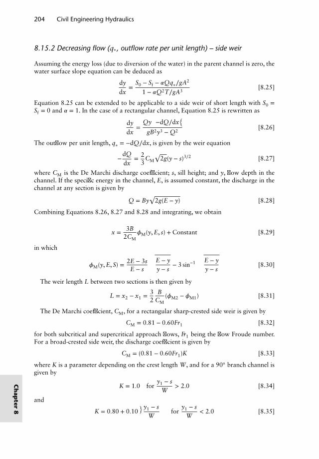
204 Civil Engineering Hydraulics
8.15.2 Decreasing flow (q∗ , outflow rate per unit length) – side weir
Assuming the energy loss (due to diversion of the water) in the parent channel is zero, thewater surface slope equation can be deduced as
dy
dx=
S0 − Sf − 𝛼Qq∗∕gA2
1 − 𝛼Q2T∕gA3[8.25]
Equation 8.25 can be extended to be applicable to a side weir of short length with S0 =Sf = 0 and 𝛼 = 1. In the case of a rectangular channel, Equation 8.25 is rewritten as
dy
dx=
Qy(−dQ∕dx
)gB2y3 − Q2
[8.26]
The outflow per unit length, q∗ = −dQ∕dx, is given by the weir equation
−dQ
dx= 2
3CM
√2g(y − s)3∕2 [8.27]
where CM is the De Marchi discharge coefficient; s, sill height; and y, flow depth in thechannel. If the specific energy in the channel, E, is assumed constant, the discharge in thechannel at any section is given by
Q = By√
2g(E − y) [8.28]
Combining Equations 8.26, 8.27 and 8.28 and integrating, we obtain
x = 3B2CM
𝜙M(y, E, s) + Constant [8.29]
in which
𝜙M(y, E, S) = 2E − 3sE − s
√E − yy − s
− 3 sin−1
√E − yy − s
[8.30]
The weir length L between two sections is then given by
L = x2 − x1 = 32
BCM
(𝜙M2 − 𝜙M1) [8.31]
The De Marchi coefficient, CM, for a rectangular sharp-crested side weir is given by
CM = 0.81 − 0.60Fr1 [8.32]
for both subcritical and supercritical approach flows, Fr1 being the flow Froude number.For a broad-crested side weir, the discharge coefficient is given by
CM = (0.81 − 0.60Fr1)K [8.33]
where K is a parameter depending on the crest length W, and for a 90◦ branch channel isgiven by
K = 1.0 fory1 − s
W> 2.0 [8.34]
and
K = 0.80 + 0.10(y1 − s
W
)for
y1 − sW
< 2.0 [8.35]
Ch
apter
8
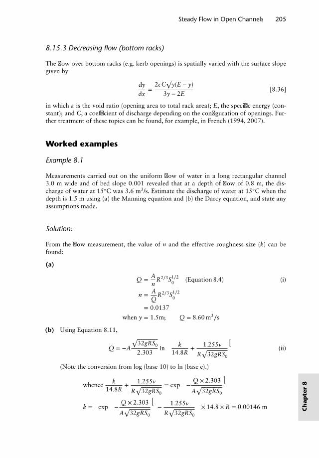
Steady Flow in Open Channels 205
8.15.3 Decreasing flow (bottom racks)
The flow over bottom racks (e.g. kerb openings) is spatially varied with the surface slopegiven by
dy
dx=
2𝜀C√
y(E − y)
3y − 2E[8.36]
in which 𝜀 is the void ratio (opening area to total rack area); E, the specific energy (con-stant); and C, a coefficient of discharge depending on the configuration of openings. Fur-ther treatment of these topics can be found, for example, in French (1994, 2007).
Worked examples
Example 8.1
Measurements carried out on the uniform flow of water in a long rectangular channel3.0 m wide and of bed slope 0.001 revealed that at a depth of flow of 0.8 m, the dis-charge of water at 15◦C was 3.6 m3/s. Estimate the discharge of water at 15◦C when thedepth is 1.5 m using (a) the Manning equation and (b) the Darcy equation, and state anyassumptions made.
Solution:
From the flow measurement, the value of n and the effective roughness size (k) can befound:
(a)
Q = An
R2∕3S1∕20 (Equation 8.4) (i)
n = AQ
R2∕3S1∕20
= 0.0137
when y = 1.5m; Q = 8.60 m3∕s
(b) Using Equation 8.11,
Q = −A
√32gRS0
2.303ln
(k
14.8R+ 1.255𝜈
R√
32gRS0
)(ii)
(Note the conversion from log (base 10) to ln (base e).)
whence k14.8R
+ 1.255𝜈
R√
32gRS0
= exp
(−
Q × 2.303
A√
32gRS0
)
k =
[exp
(−
Q × 2.303
A√
32gRS0
)− 1.255𝜈
R√
32gRS0
]× 14.8 × R = 0.00146 m C
hap
ter
8
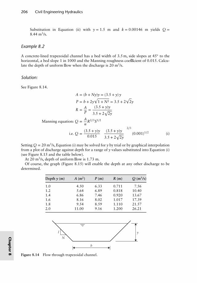
206 Civil Engineering Hydraulics
Substitution in Equation (ii) with y = 1.5 m and k = 0.00146 m yields Q =8.44 m3/s.
Example 8.2
A concrete-lined trapezoidal channel has a bed width of 3.5 m, side slopes at 45◦ to thehorizontal, a bed slope 1 in 1000 and the Manning roughness coefficient of 0.015. Calcu-late the depth of uniform flow when the discharge is 20 m3/s.
Solution:
See Figure 8.14.
A = (b + Ny)y = (3.5 + y) y
P = b + 2y√
1 + N2 = 3.5 + 2√
2y
R = AP
=(3.5 + y)y
3.5 + 2√
2y
Manning equation: Q = An
R2∕3S1∕2
i.e. Q =(3.5 + y)y
0.015
[(3.5 + y)y
3.5 + 2√
2y
]2∕3
(0.001)1∕2 (i)
Setting Q = 20 m3/s, Equation (i) may be solved for y by trial or by graphical interpolationfrom a plot of discharge against depth for a range of y values substituted into Equation (i)(see Figure 8.15 and the table below).
At 20 m3/s, depth of uniform flow is 1.73 m.Of course, the graph (Figure 8.15) will enable the depth at any other discharge to be
determined.
Depth y (m) A (m2) P (m) R (m) Q (m3/s)
1.0 4.50 6.33 0.711 7.561.2 5.64 6.89 0.818 10.401.4 6.86 7.46 0.920 13.671.6 8.16 8.02 1.017 17.391.8 9.54 8.59 1.110 21.572.0 11.00 9.16 1.200 26.21
N
y
b
l
Figure 8.14 Flow through trapezoidal channel.
Ch
apter
8
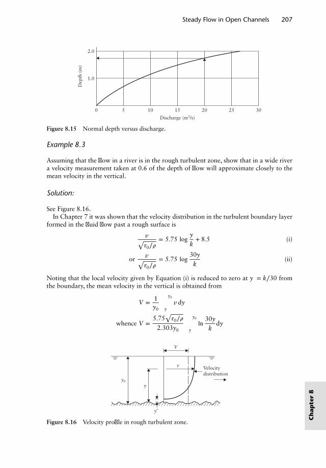
Steady Flow in Open Channels 207
0
1.0D
epth
(m
)
2.0
15105
Discharge (m3/s)
302520
Figure 8.15 Normal depth versus discharge.
Example 8.3
Assuming that the flow in a river is in the rough turbulent zone, show that in a wide rivera velocity measurement taken at 0.6 of the depth of flow will approximate closely to themean velocity in the vertical.
Solution:
See Figure 8.16.In Chapter 7 it was shown that the velocity distribution in the turbulent boundary layer
formed in the fluid flow past a rough surface is
v√𝜏0∕𝜌
= 5.75 logy
k+ 8.5 (i)
or v√𝜏0∕𝜌
= 5.75 log30y
k(ii)
Noting that the local velocity given by Equation (i) is reduced to zero at y′ = k∕30 fromthe boundary, the mean velocity in the vertical is obtained from
V = 1y0 ∫
y0
y′v dy
whence V =5.75
√𝜏0∕𝜌
2.303y0 ∫y0
y′ln
30y
kdy
V
v
y
y′
y0
Velocitydistribution
Figure 8.16 Velocity profile in rough turbulent zone.
Ch
apte
r8
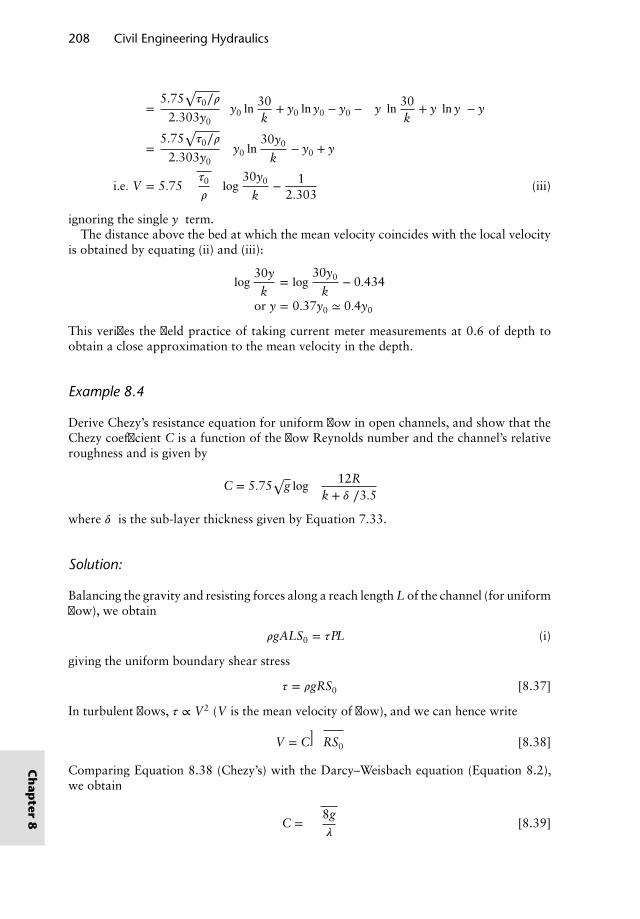
208 Civil Engineering Hydraulics
=5.75
√𝜏0∕𝜌
2.303y0
[y0 ln
30k
+ y0 ln y0 − y0 −(
y′ ln 30k
+ y′ ln y′ − y′)]
=5.75
√𝜏0∕𝜌
2.303y0
(y0 ln
30y0
k− y0 + y′
)
i.e. V = 5.75√𝜏0
𝜌
(log
30y0
k− 1
2.303
)(iii)
ignoring the single y′ term.The distance above the bed at which the mean velocity coincides with the local velocity
is obtained by equating (ii) and (iii):
log30y
k= log
30y0
k− 0.434
or y = 0.37y0 ≃ 0.4y0
This verifies the field practice of taking current meter measurements at 0.6 of depth toobtain a close approximation to the mean velocity in the depth.
Example 8.4
Derive Chezy’s resistance equation for uniform flow in open channels, and show that theChezy coefficient C is a function of the flow Reynolds number and the channel’s relativeroughness and is given by
C = 5.75√
g log(
12Rk + 𝛿′∕3.5
)
where 𝛿′ is the sub-layer thickness given by Equation 7.33.
Solution:
Balancing the gravity and resisting forces along a reach length L of the channel (for uniformflow), we obtain
𝜌gALS0 = 𝜏PL (i)
giving the uniform boundary shear stress
𝜏 = 𝜌gRS0 [8.37]
In turbulent flows, 𝜏 ∝ V2 (V is the mean velocity of flow), and we can hence write
V = C√
RS0 [8.38]
Comparing Equation 8.38 (Chezy’s) with the Darcy–Weisbach equation (Equation 8.2),we obtain
C =√
8g𝜆
[8.39]
Ch
apter
8
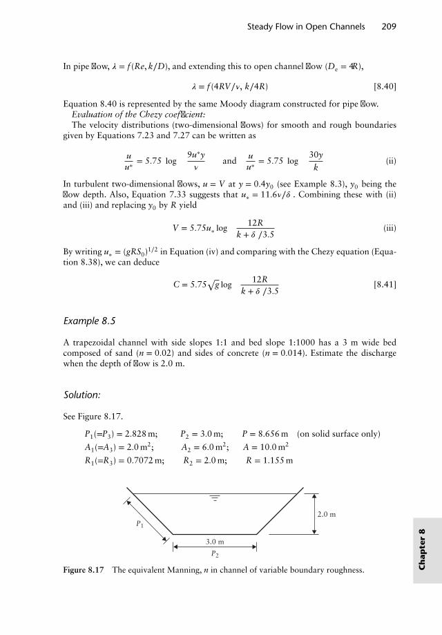
Steady Flow in Open Channels 209
In pipe flow, 𝜆 = f (Re, k∕D), and extending this to open channel flow (De = 4R),
𝜆 = f (4RV∕𝜈, k∕4R) [8.40]
Equation 8.40 is represented by the same Moody diagram constructed for pipe flow.Evaluation of the Chezy coefficient:The velocity distributions (two-dimensional flows) for smooth and rough boundaries
given by Equations 7.23 and 7.27 can be written as
uu∗ = 5.75 log
(9u∗y𝜈
)and u
u∗ = 5.75 log(
30y
k
)(ii)
In turbulent two-dimensional flows, u = V at y = 0.4y0 (see Example 8.3), y0 being theflow depth. Also, Equation 7.33 suggests that u∗ = 11.6𝜈∕𝛿′. Combining these with (ii)and (iii) and replacing y0 by R yield
V = 5.75u∗ log(
12Rk + 𝛿′∕3.5
)(iii)
By writing u∗ = (gRS0)1∕2 in Equation (iv) and comparing with the Chezy equation (Equa-tion 8.38), we can deduce
C = 5.75√
g log(
12Rk + 𝛿′∕3.5
)[8.41]
Example 8.5
A trapezoidal channel with side slopes 1:1 and bed slope 1:1000 has a 3 m wide bedcomposed of sand (n = 0.02) and sides of concrete (n = 0.014). Estimate the dischargewhen the depth of flow is 2.0 m.
Solution:
See Figure 8.17.
P1(=P3) = 2.828 m; P2 = 3.0 m; P = 8.656 m (on solid surface only)
A1(=A3) = 2.0 m2; A2 = 6.0 m2; A = 10.0 m2
R1(=R3) = 0.7072 m; R2 = 2.0 m; R = 1.155 m
3.0 m
P2
P1
2.0 m
Figure 8.17 The equivalent Manning, n in channel of variable boundary roughness. Ch
apte
r8
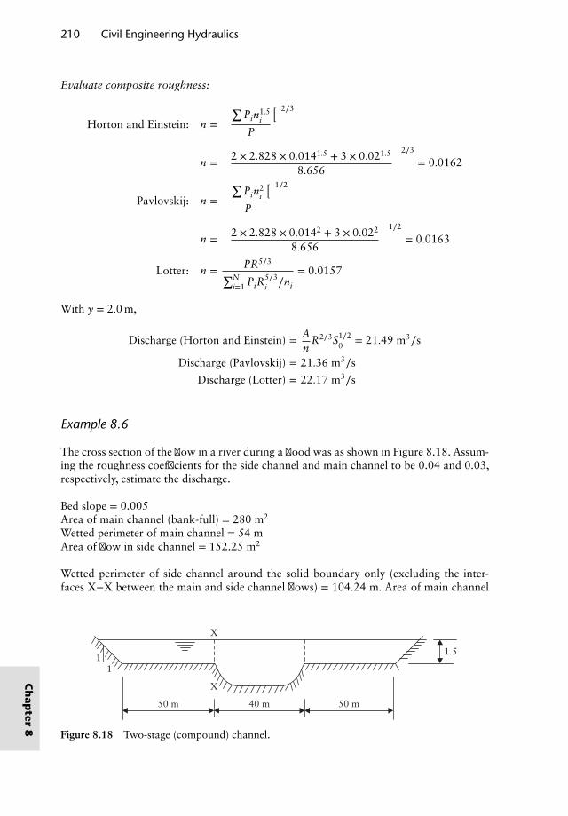
210 Civil Engineering Hydraulics
Evaluate composite roughness:
Horton and Einstein: n =
(∑Pin
1.5i
P
)2∕3
n =(
2 × 2.828 × 0.0141.5 + 3 × 0.021.5
8.656
)2∕3
= 0.0162
Pavlovskij: n =
(∑Pin
2i
P
)1∕2
n =(
2 × 2.828 × 0.0142 + 3 × 0.022
8.656
)1∕2
= 0.0163
Lotter: n = PR5∕3∑Ni=1 PiR
5∕3i ∕ni
= 0.0157
With y = 2.0 m,
Discharge (Horton and Einstein) = An
R2∕3S1∕20 = 21.49 m3∕s
Discharge (Pavlovskij) = 21.36 m3∕s
Discharge (Lotter) = 22.17 m3∕s
Example 8.6
The cross section of the flow in a river during a flood was as shown in Figure 8.18. Assum-ing the roughness coefficients for the side channel and main channel to be 0.04 and 0.03,respectively, estimate the discharge.
Bed slope = 0.005Area of main channel (bank-full) = 280 m2
Wetted perimeter of main channel = 54 mArea of flow in side channel = 152.25 m2
Wetted perimeter of side channel around the solid boundary only (excluding the inter-faces X−X between the main and side channel flows) = 104.24 m. Area of main channel
X
X
40 m50 m
11
50 m
1.5
Figure 8.18 Two-stage (compound) channel.
Ch
apter
8
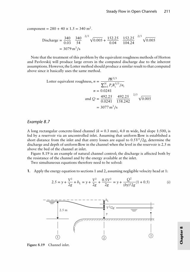
Steady Flow in Open Channels 211
component = 280 + 40 × 1.5 = 340 m2.
Discharge = 3400.03
(34054
)2∕3 √0.005 + 152.25
0.04
(152.25104.24
)2∕3 √0.005
= 3079 m3∕s
Note that the treatment of this problem by the equivalent roughness methods of Hortonand Pavlovskij will produce large errors in the computed discharge due to the inherentassumptions. However, the Lotter method should produce a similar result to that computedabove since it basically uses the same method.
Lotter equivalent roughness, n = PR5∕3∑Ni=1 PiR
5∕3i ∕ni
n = 0.0241
and Q = 492.250.0241
(492.25158.242
)2∕3 √0.005
= 3077 m3∕s
Example 8.7
A long rectangular concrete-lined channel (k = 0.3 mm), 4.0 m wide, bed slope 1:500, isfed by a reservoir via an uncontrolled inlet. Assuming that uniform flow is established ashort distance from the inlet and that entry losses are equal to 0.5V2∕2g, determine thedischarge and depth of uniform flow in the channel when the level in the reservoir is 2.5 mabove the bed of the channel at inlet.
Figure 8.19 is an example of natural channel control; the discharge is affected both bythe resistance of the channel and by the energy available at the inlet.
Two simultaneous equations therefore need to be solved:
1. Apply the energy equation to sections 1 and 2, assuming negligible velocity head at 1:
2.5 = y + V2
2g+ hL = y + V2
2g+ 0.5V2
2g= y +
Q2
(by)22g(1 + 0.5) (i)
2.5 my
hL
V2/2g
1 23
Figure 8.19 Channel inlet. Ch
apte
r8
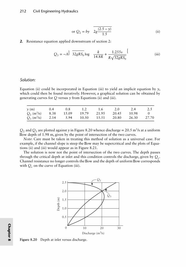
212 Civil Engineering Hydraulics
or Q2 = by
√2g
(2.5 − y)1.5
(ii)
2. Resistance equation applied downstream of section 2:
Q3 = −A√
32gRS0 log
(k
14.8R+ 1.255𝜈
R√
32gRS0
)(iii)
Solution:
Equation (ii) could be incorporated in Equation (iii) to yield an implicit equation by y,which could then be found iteratively. However, a graphical solution can be obtained bygenerating curves for Q versus y from Equations (ii) and (iii).
y (m) 0.4 0.8 1.2 1.6 2.0 2.4 2.5Q2 (m3/s) 8.38 15.09 19.79 21.95 20.45 10.98 0Q3 (m3/s) 2.14 5.94 10.50 15.51 20.80 26.30 27.70
Q2 and Q3 are plotted against y in Figure 8.20 whence discharge = 20.5 m3/s at a uniformflow depth of 1.98 m, given by the point of intersection of the two curves.
Note: Care must be taken in treating this method of solution as a universal case. Forexample, if the channel slope is steep the flow may be supercritical and the plots of Equa-tions (ii) and (iii) would appear as in Figure 8.21.
The solution is now not the point of intersection of the two curves. The depth passesthrough the critical depth at inlet and this condition controls the discharge, given by Qc.Channel resistance no longer controls the flow and the depth of uniform flow correspondswith Qc on the curve of Equation (iii).
Q22.5
2.0
1.5
Dep
th (
m)
1.0
0.5
0 10
Discharge (m3/s)
3020
Q3
Figure 8.20 Depth at inlet versus discharge.
Ch
apter
8
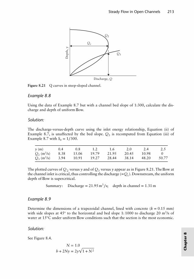
Steady Flow in Open Channels 213
Discharge, Q
Qc
Q2
Q3
Dep
th, y
Figure 8.21 Q curves in steep-sloped channel.
Example 8.8
Using the data of Example 8.7 but with a channel bed slope of 1:300, calculate the dis-charge and depth of uniform flow.
Solution:
The discharge-versus-depth curve using the inlet energy relationship, Equation (ii) ofExample 8.7, is unaffected by the bed slope. Q3 is recomputed from Equation (iii) ofExample 8.7 with S0 = 1∕300.
y (m) 0.4 0.8 1.2 1.6 2.0 2.4 2.5Q2 (m3/s) 8.38 15.06 19.79 21.95 20.45 10.98 0Q3 (m3/s) 3.94 10.91 19.27 28.44 38.14 48.20 50.77
The plotted curves of Q 2 versus y and of Q3 versus y appear as in Figure 8.21. The flow atthe channel inlet is critical, thus controlling the discharge (=Qc). Downstream, the uniformdepth of flow is supercritical.
Summary: Discharge = 21.95 m3∕s; depth in channel = 1.31 m
Example 8.9
Determine the dimensions of a trapezoidal channel, lined with concrete (k = 0.15 mm)with side slopes at 45◦ to the horizontal and bed slope 1: 1000 to discharge 20 m3/s ofwater at 15◦C under uniform flow conditions such that the section is the most economic.
Solution:
See Figure 8.4.
N = 1.0
b + 2Ny = 2y√
1 + N 2 Ch
apte
r8
214 Civil Engineering Hydraulics
b + 2y = 2√
2y
or b = 0.828y
Then A = 1.828y2; P = 3.656y
Q = −A√
32gRS0 log
(k
14.8R+ 1.255𝜈
R√
32gRS0
)
This must be solved by trial, calculating Q for a series of y.
y (m) 0.5 1.0 1.5 1.8 1.9 2.0Q (m3/s) 0.54 3.30 9.50 15.26 17.56 20.06
Adopt y = 2.0 m, then
b = 1.414 m
Example 8.10
A trapezoidal irrigation channel excavated in silty sand having a critical tractive force onthe horizontal of 2.4 N/m2 and angle of friction 30◦ is to be designed to convey a dischargeof 10 m3/s on a bed slope of 1:10 000. The side slopes will be 1 (vertical) : 2 (horizontal)(n = 0.02).
Solution:
The channel bed is almost horizontal and the critical tractive force on the bed may thereforebe taken as 2.4 N/m2.
The limiting tractive force on the sides is
𝜏cs = 𝜏cb
√1 − sin2
𝜃
sin2𝜙
(see Section 8.5.1)
= 2.4
√1 − sin2(26.565◦)
sin2(30◦)
= 2.4√
1 − 0.8 = 1.073 N∕m2
⇒ 0.76𝜌gyS0 >| 1.073 N∕m2
⇒ y >| 1.0730.76 × 1000 × 9.81 × 0.0001
y >| 1.44 m
Now Q = An
R2∕3S1∕20
10 =(b + 2y)y
n
((b + 2y)y
b + 2y√
5
)2∕3
S1∕20
Ch
apter
8
Steady Flow in Open Channels 215
10 = (b + 2.88) × 1.440.02
((b + 2.88) × 1.44
b + 6.44
)2∕3
×√
0.0001
Solving by trial (graphical interpolation) for series of values of b,
b 1.0 2.0 4.0 8.0 10.0 12.0RHS 2.31 3.11 4.78 8.27 10.05 11.84
required b = 9.95 m
V = 0.54 m∕s
which agrees reasonably with the maximum mean velocity criterion (Table 8.3).
Example 8.11 (Maximum mean velocity criterion)
Using the data of the previous example, determine the channel dimensions such that themean velocity does not exceed 0.5 m/s when conveying the discharge of 10 m3/s.
Solution:
Q = AV; 10 = A × 0.5
whence A = 20 m2
and A = (b + 2y)y
whence b = (20∕y) − 2y
Q = An
R2∕3S1∕20 = A5∕3
nP2∕3S1∕2
i.e. 10 =205∕3 ×
√0.0001
0.02 × P2∕3
whence P = 20 m
and P = b + 2y√
5 = 20y
+ 2y(√
5 − 1)
that is, 2.472y2 − 20y + 20 = 0
whence y = 1.169 m
and b = 14.77 m
Example 8.12
Check the proposed design of a branch of a wastewater sewerage system receiving the flowfrom 300 houses. The pipe is 150 mm in diameter with a proposed slope of 1 in 100. Theroughness of the sewer is 1.5 mm. The average flow, known as dry weather flow (DWF),is calculated assuming a population of 3 person per house, a flow of 200 L/day per person C
hap
ter
8
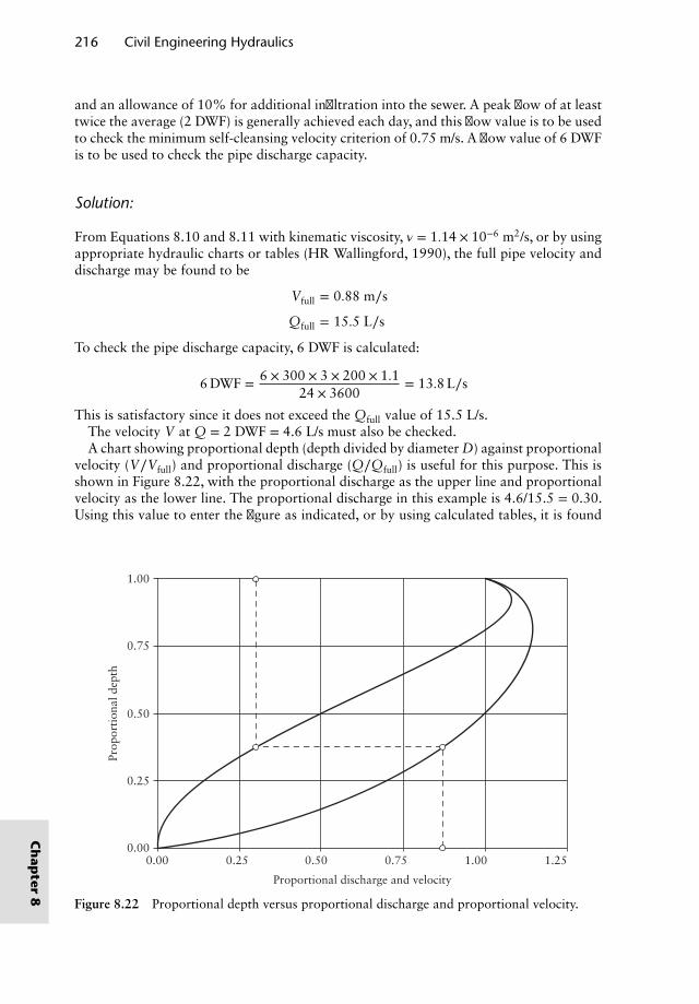
216 Civil Engineering Hydraulics
and an allowance of 10% for additional infiltration into the sewer. A peak flow of at leasttwice the average (2 DWF) is generally achieved each day, and this flow value is to be usedto check the minimum self-cleansing velocity criterion of 0.75 m/s. A flow value of 6 DWFis to be used to check the pipe discharge capacity.
Solution:
From Equations 8.10 and 8.11 with kinematic viscosity, 𝜈 = 1.14 × 10⁻⁶ m2/s, or by usingappropriate hydraulic charts or tables (HR Wallingford, 1990), the full pipe velocity anddischarge may be found to be
Vfull = 0.88 m∕s
Qfull = 15.5 L∕s
To check the pipe discharge capacity, 6 DWF is calculated:
6 DWF = 6 × 300 × 3 × 200 × 1.124 × 3600
= 13.8 L∕s
This is satisfactory since it does not exceed the Qfull value of 15.5 L/s.The velocity V at Q = 2 DWF = 4.6 L/s must also be checked.A chart showing proportional depth (depth divided by diameter D) against proportional
velocity (V∕Vfull) and proportional discharge (Q∕Qfull) is useful for this purpose. This isshown in Figure 8.22, with the proportional discharge as the upper line and proportionalvelocity as the lower line. The proportional discharge in this example is 4.6/15.5 = 0.30.Using this value to enter the figure as indicated, or by using calculated tables, it is found
0.00
0.25
0.50
0.75
1.00
1.251.000.750.500.250.00
Proportional discharge and velocity
Prop
orti
onal
dep
th
Figure 8.22 Proportional depth versus proportional discharge and proportional velocity.
Ch
apter
8
Steady Flow in Open Channels 217
that the proportional depth is 0.38 and the corresponding proportional velocity is 0.87.The velocity at 2 DWF is therefore given by
V =(
VVfull
)Vfull = 0.87 × 0.88 m∕s = 0.77 m∕s
The design is therefore satisfactory since this exceeds the required self-cleansing velocityof 0.75 m/s.
Example 8.13
Design a branch within a storm sewer network which has a length of 100 m, a bed slopeof 1 in 125 and a roughness size of 0.6 mm and which receives the storm runoff from3.5 ha of impermeable surface using the rational method. In designing the upstream pipes,the maximum ‘time of concentration’ at the head of the pipe has been found to be 6.2min. Use the relationship between rainfall intensity and average storm duration tabulatedbelow.
Storm duration (min) 6.0 7.0 8.0Average rainfall intensity (mm/h) 61.4 57.2 53.5
Notes: The rational method gives the peak discharge (Qp) from an urbanised catchmentin the form
Qp = 1360
Ai (m3∕s)
where A is the impermeable area (ha) assuming 100% runoff; and i is the average rainfallintensity (mm∕h) during the storm.
Since the average rainfall intensity of storms of a given average return period decreaseswith increase in storm duration, the critical design storm is that which has a duration equalto the ‘time of concentration of the catchment’, tc. tc is the longest time of travel of a liquidelement to the point in question in the catchment and includes the times of overland andpipe flow; the time of pipe flow is based on full-bore velocities. For further coverage ofdesign rainfall data see, for example, Mansell (2003).
Solution:
The selection of the appropriate pipe diameter is by trial and improvement. Try D =500 mm.
Full-bore conditions are found in a similar way to the previous example:
Vfull = 1.94 m∕s
Qfull = 0.38 m3∕s
Travel time along pipe = 1001.94 × 60
= 0.9 min Ch
apte
r8
218 Civil Engineering Hydraulics
Thus tc = 6.2 + 0.9 = 7.1 min;
whence i = 56.8 mm∕h
⇒ Qp = 3.5 × 56.8360
= 0.55 m3∕s
This is greater than the full-bore discharge (Qfull) of the 500 mm diameter pipe which istherefore too small. Try 600 mm diameter pipe.
Vfull = 2.18 m∕s
Qfull = 0.62 m3∕s
Travel time along pipe = 1002.18 × 60
= 0.8 min
tc = 7.0 min; whence i = 57.2 mm∕h
Qp = 3.5 × 57.2360
= 0.56 m3∕s
This does not exceed the full-bore discharge capacity, and so a 600 mm diameter sewer isa satisfactory design without surcharging.
Example 8.14
A rectangular channel 5 m wide laid to a mild bed slope conveys a discharge of 8 m3/s ata uniform flow depth of 1.25 m.
(a) Determine the critical depth.(b) Neglecting the energy loss, show how the height of a streamlined sill constructed
on the bed affects the depth upstream of the sill and the depth at the crest of thesill.
(c) Show that if the flow at the crest becomes critical, the structure can be used as aflow-measuring device using only an upstream depth measurement.
Solution:
(a)
yc = 3
√q2
g; q = 8
5= 1.6 m3∕(s m)
yc = 3
√1.62
9.81= 0.639 m
(b) Neglecting losses between 1 and 2 (see Figure 8.23),
E1 = E2 + z
In the case of a uniform rectangular channel the specific energy curve is the same for anysection, and if this is drawn for the specified discharge it can be used to show the variationof y1 and y2.
Ch
apter
8
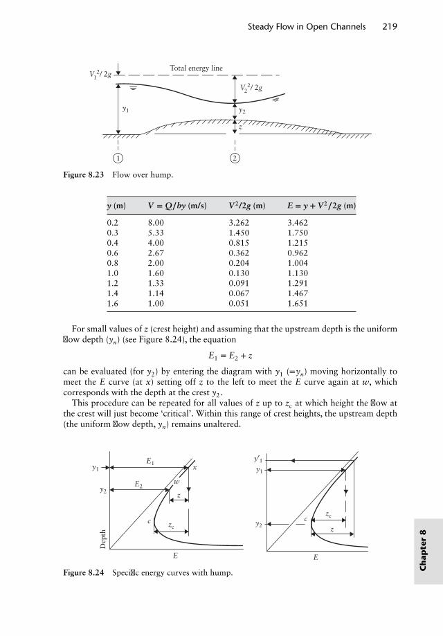
Steady Flow in Open Channels 219
V12/ 2g
Total energy line
y1 y2
z
V22/ 2g
1 2
Figure 8.23 Flow over hump.
y (m) V = Q∕by (m/s) V2/2g (m) E = y + V2∕2g (m)
0.2 8.00 3.262 3.4620.3 5.33 1.450 1.7500.4 4.00 0.815 1.2150.6 2.67 0.362 0.9620.8 2.00 0.204 1.0041.0 1.60 0.130 1.1301.2 1.33 0.091 1.2911.4 1.14 0.067 1.4671.6 1.00 0.051 1.651
For small values of z (crest height) and assuming that the upstream depth is the uniformflow depth (yn) (see Figure 8.24), the equation
E1 = E2 + z
can be evaluated (for y2) by entering the diagram with y1 (=yn) moving horizontally tomeet the E curve (at x) setting off z to the left to meet the E curve again at w, whichcorresponds with the depth at the crest y2.
This procedure can be repeated for all values of z up to zc at which height the flow atthe crest will just become ‘critical’. Within this range of crest heights, the upstream depth(the uniform flow depth, yn) remains unaltered.
E1
E2
E E
y2
y1
y′1
y2
y1
z
zc c
Dep
th
x
zc
zc
w
Figure 8.24 Specific energy curves with hump. Ch
apte
r8
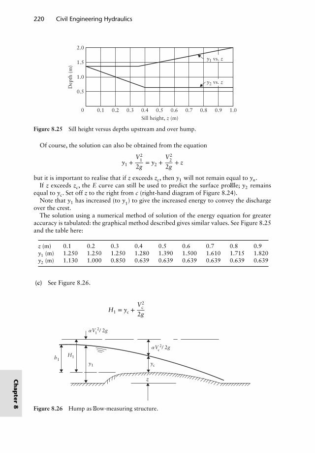
220 Civil Engineering Hydraulics
2.0
1.5
1.0
0.5
0 0.50.40.30.20.1
Sill height, z (m)
Dep
th (
m)
1.00.90.80.70.6
y1 vs. z
y2 vs. z
Figure 8.25 Sill height versus depths upstream and over hump.
Of course, the solution can also be obtained from the equation
y1 +V2
1
2g= y2 +
V22
2g+ z
but it is important to realise that if z exceeds zc, then y1 will not remain equal to yn.If z exceeds zc, the E curve can still be used to predict the surface profile; y2 remains
equal to yc. Set off z to the right from c (right-hand diagram of Figure 8.24).Note that y1 has increased (to y′1) to give the increased energy to convey the discharge
over the crest.The solution using a numerical method of solution of the energy equation for greater
accuracy is tabulated: the graphical method described gives similar values. See Figure 8.25and the table here:
z (m) 0.1 0.2 0.3 0.4 0.5 0.6 0.7 0.8 0.9y1 (m) 1.250 1.250 1.250 1.280 1.390 1.500 1.610 1.715 1.820y2 (m) 1.130 1.000 0.850 0.639 0.639 0.639 0.639 0.639 0.639
(c) See Figure 8.26.
H1 = yc +V2
c
2g
z
ycy1
H1h1
αVc2/ 2g
αV12/ 2g
Figure 8.26 Hump as flow-measuring structure.
Ch
apter
8
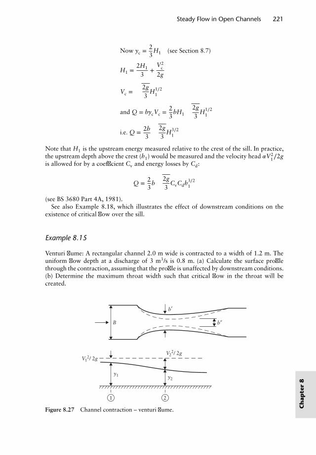
Steady Flow in Open Channels 221
Now yc =23
H1 (see Section 8.7)
H1 =2H1
3+
V2c
2g
Vc =√
2g3
H1∕21
and Q = bycVc =23
bH1
√2g3
H1∕21
i.e. Q = 2b3
√2g3
H3∕21
Note that H1 is the upstream energy measured relative to the crest of the sill. In practice,the upstream depth above the crest (h1) would be measured and the velocity head 𝛼V2
1∕2gis allowed for by a coefficient Cv and energy losses by Cd:
Q = 23
b
√2g3
CvCdh3∕21
(see BS 3680 Part 4A, 1981).See also Example 8.18, which illustrates the effect of downstream conditions on the
existence of critical flow over the sill.
Example 8.15
Venturi flume: A rectangular channel 2.0 m wide is contracted to a width of 1.2 m. Theuniform flow depth at a discharge of 3 m3/s is 0.8 m. (a) Calculate the surface profilethrough the contraction, assuming that the profile is unaffected by downstream conditions.(b) Determine the maximum throat width such that critical flow in the throat will becreated.
b′
B
y1 y2
V12/ 2g
V22/ 2g
b″
1 2
Figure 8.27 Channel contraction – venturi flume. Ch
apte
r8
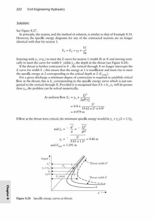
222 Civil Engineering Hydraulics
Solution:
See Figure 8.27.In principle, the system, and the method of solution, is similar to that of Example 8.14.
However, the specific energy diagrams for any of the contracted sections are no longeridentical with that for section 1.
E1 = E2 = y2 +V2
2
2g
Entering with y1 (=yn) to meet the E curve for section 1 (width B) at X and moving verti-cally to meet the curve for width b′ yields y′2, the depth in the throat (see Figure 8.28).
If the throat is further contracted to b′′, the vertical through X no longer intercepts theE curve for width b′′; this means that the energy at 1 is insufficient and must rise to meetthe specific energy at 2 corresponding to the critical depth at 2 (E2min).
For a given discharge a minimum degree of contraction is required to establish criticalflow at the throat; this is bc corresponding to the specific energy curve which is just tan-gential to the vertical through X. Provided it is recognised that if b < bc, y1 will be greaterthan yn, the problem can be solved numerically.
At uniform flow E1 = yn +Q 2
2gB2y2n
= 0.8 + 32
19.62 × 22 × 0.82
= 0.979 m
If flow at the throat were critical, the minimum specific energy would be yc + yc∕2 = 1.5yc
and yc = 3
√q2
g= 3
√Q2
gb2
yc = 3
√32
9.81 × 1.22= 0.86 m
and Emin = 1.291 m
E
B
Throat width b′
Depth
Throat width b″y1″y1 (=yn)
y2(c)y2
E1
E2 (min)
X
Figure 8.28 Specific energy curves at throat.
Ch
apter
8
Steady Flow in Open Channels 223
This is greater than the energy upstream at uniform flow; thus, the flow in the throat willbe critical.
Therefore, y2 = 0.86 m and y1 is obtained from
1.291 = y1 +Q 2
2gB2y21
1.291 = y1 +32
19.62 × 22 × y21
whence y1 = 1.215 m
(b) Let bc be the throat width to create critical flow at the specified discharge. Critical flowcan just be achieved with the upstream energy of 0.979 m.
0.979 = yc +Q 2
2gb2c y2
c
(i)
Since 0.979 m is also the energy corresponding to the critical flow at the throat,
yc = 2∕3 × 0.979 = 0.653 mwhence from Equation (i)
0.326 = 32
19.62 × b2c × 0.6532
The solution to which is bc = 1.816 m.Note: In a similar manner to that of Example 8.14(c), it can be shown that if the flow inthe throat is critical, the discharge can be calculated from the theoretical equation
Q = 23
√2g3
bH3∕21
(Practical form: Q = 2
3
√2g3
bCvCdh3∕21
)
where H1 is the upstream energy (h1 + V21∕2g) and h1 the upstream depth. In practice,
the throat would be made narrower than that calculated in the example above in orderto create supercritical flow conditions in the expanding section downstream of the throatfollowed by a hydraulic jump in the downstream channel. The reader is referred to BS3680 Part 4C (1981) and also to Example 8.19.
Example 8.16
A vertical sluice gate with an opening of 0.67 m produces a downstream jet depth of 0.40m when installed in a long rectangular channel 5.0 m wide conveying a steady dischargeof 20.0 m3/s. Assuming that the flow downstream of the gate eventually returns to theuniform flow depth of 2.5 m,
(a) verify that a hydraulic jump occurs. Assume 𝛼 = 𝛽 = 1.0.(b) calculate the head loss in the jump.(c) if the head loss through the gate is 0.05V2
J ∕2g, calculate the depth upstream of thegate and the force on the gate.
(d) if the downstream depth is increased to 3.0 m, analyse the flow conditions at the gate. Ch
apte
r8
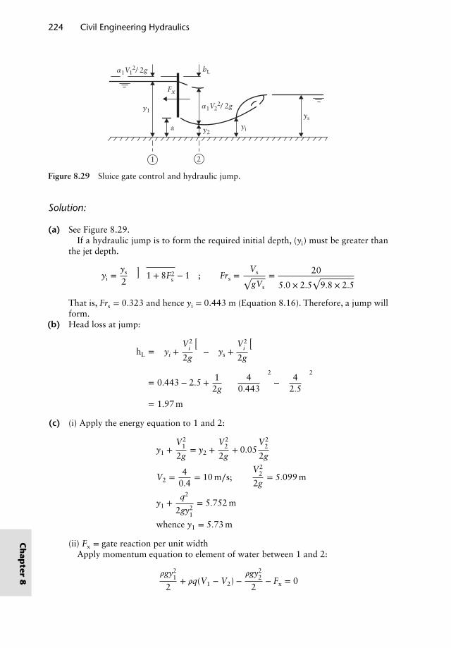
224 Civil Engineering Hydraulics
y1
y2yi
ys
a
hL
Fx
α1V12/ 2g
α1V22/ 2g
1 2
Figure 8.29 Sluice gate control and hydraulic jump.
Solution:
(a) See Figure 8.29.If a hydraulic jump is to form the required initial depth, (yi) must be greater than
the jet depth.
yi =ys
2
(√1 + 8F2
s − 1)
; Frs =Vs√gVs
= 20
5.0 × 2.5√
9.8 × 2.5
That is, Frs = 0.323 and hence yi = 0.443 m (Equation 8.16). Therefore, a jump willform.
(b) Head loss at jump:
hL =
(yi +
V2i
2g
)−
(ys +
V2i
2g
)
= 0.443 − 2.5 + 12g
[(4
0.443
)2
−(
42.5
)2]
= 1.97 m
(c) (i) Apply the energy equation to 1 and 2:
y1 +V2
1
2g= y2 +
V22
2g+ 0.05
V22
2g
V2 = 40.4
= 10 m∕s;V2
2
2g= 5.099 m
y1 +q2
2gy21
= 5.752 m
whence y1 = 5.73 m
(ii) Fx = gate reaction per unit widthApply momentum equation to element of water between 1 and 2:
𝜌gy21
2+ 𝜌q(V1 − V2) −
𝜌gy22
2− Fx = 0
Ch
apter
8
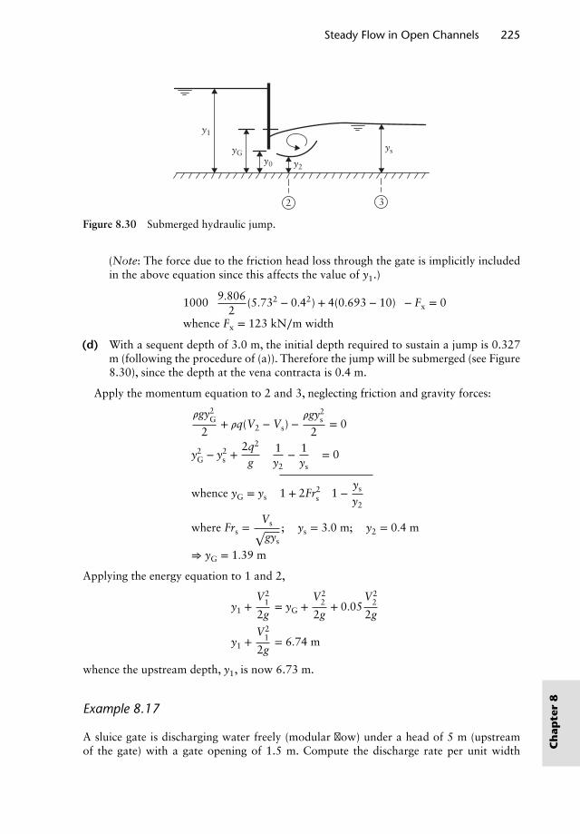
Steady Flow in Open Channels 225
yGy0
y1
y2
ys
2 3
Figure 8.30 Submerged hydraulic jump.
(Note: The force due to the friction head loss through the gate is implicitly includedin the above equation since this affects the value of y1.)
1000[
9.8062
(5.732 − 0.42) + 4(0.693 − 10)]− Fx = 0
whence Fx = 123 kN∕m width
(d) With a sequent depth of 3.0 m, the initial depth required to sustain a jump is 0.327m (following the procedure of (a)). Therefore the jump will be submerged (see Figure8.30), since the depth at the vena contracta is 0.4 m.
Apply the momentum equation to 2 and 3, neglecting friction and gravity forces:
𝜌gy2G
2+ 𝜌q(V2 − Vs) −
𝜌gy2s
2= 0
y2G − y2
s +2q2
g
(1y2
− 1ys
)= 0
whence yG = ys
√1 + 2Fr2
s
(1 −
ys
y2
)
where Frs =Vs√gys
; ys = 3.0 m; y2 = 0.4 m
⇒ yG = 1.39 m
Applying the energy equation to 1 and 2,
y1 +V2
1
2g= yG +
V22
2g+ 0.05
V22
2g
y1 +V2
1
2g= 6.74 m
whence the upstream depth, y1, is now 6.73 m.
Example 8.17
A sluice gate is discharging water freely (modular flow) under a head of 5 m (upstreamof the gate) with a gate opening of 1.5 m. Compute the discharge rate per unit width C
hap
ter
8
226 Civil Engineering Hydraulics
of the gate. If the water depth immediately downstream of the gate is 2 m (drowned ornon-modular flow), determine the discharge rate.
Solution:
Referring to Figure 8.29 for the modular/free flow case,
q = Cda√
2gy1 (8.42)
where
Cd =Cc√
1 + Cc a∕y1
(8.43)
The contraction coefficient Cc (=y2∕a) is a function of a∕y1; a reasonable constant valueof Cc = 0.60 may be assumed for most conditions. Equation 8.42 can also be written as
q = C′da√
2g(y1 − Cca) (8.44)
where
C′d =
Cc√1 −
(Cc a∕y1
)2(8.45)
For the submerged (non-modular) flow condition, the discharge
qs = C′dsa
√2g(y1 − yG) (8.46)
where C′ds= C′
dwith Cc = 0.60. The depth of submergence, yG, downstream of the gate
(see Figure 8.30) is computed by the momentum equation (see Example 8.16) as
yG
ys=
√1 + Fr2
s
(1 −
ys
Cca
)(8.47)
(i) Modular flow:ay1
= 0.3
⇒ Cd = 0.552 (Equation 8.43)
hence q = 8.2 m3∕(s m) (Equation 8.42)
(ii) Non-modular flow:
C′ds= C′
d= 0.610 (Equation 8.45)
⇒ q = 0.61 × 1.5 ×√
2g(5 − 2) = 7.08 m3∕(s m)
Note: If we assume that the flow condition immediately downstream of the gate remainsunaffected by submergence, we can obtain V1 by the energy and continuity equations.
5 +V2
1
2g= 2 +
V22
2g; 5V1 = 0.6 × 1.5V2
as V1 = 1.4 m∕s; hence q = y1 × V1 = 7.0 m3∕(s m)
Ch
apter
8
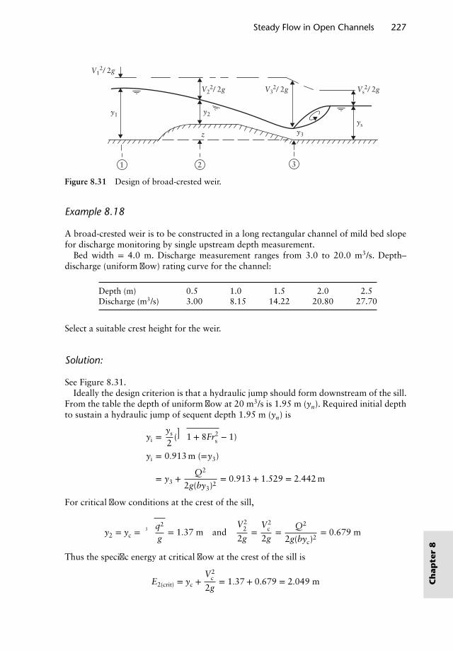
Steady Flow in Open Channels 227
y2
z y3
ys
y1
V12/ 2g
V22/ 2g V3
2/ 2g Vs2/ 2g
321
Figure 8.31 Design of broad-crested weir.
Example 8.18
A broad-crested weir is to be constructed in a long rectangular channel of mild bed slopefor discharge monitoring by single upstream depth measurement.
Bed width = 4.0 m. Discharge measurement ranges from 3.0 to 20.0 m3/s. Depth–discharge (uniform flow) rating curve for the channel:
Depth (m) 0.5 1.0 1.5 2.0 2.5Discharge (m3/s) 3.00 8.15 14.22 20.80 27.70
Select a suitable crest height for the weir.
Solution:
See Figure 8.31.Ideally the design criterion is that a hydraulic jump should form downstream of the sill.
From the table the depth of uniform flow at 20 m3/s is 1.95 m (yn). Required initial depthto sustain a hydraulic jump of sequent depth 1.95 m (yn) is
yi =ys
2(√
1 + 8Fr2s − 1)
yi = 0.913 m (=y3)
= y3 +Q2
2g(by3)2= 0.913 + 1.529 = 2.442 m
For critical flow conditions at the crest of the sill,
y2 = yc =3
√q2
g= 1.37 m and
V22
2g=
V2c
2g=
Q2
2g(byc)2= 0.679 m
Thus the specific energy at critical flow at the crest of the sill is
E2(crit) = yc +V2
c
2g= 1.37 + 0.679 = 2.049 m C
hap
ter
8
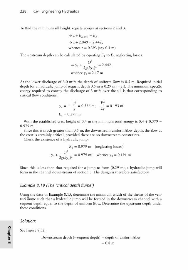
228 Civil Engineering Hydraulics
To find the minimum sill height, equate energy at sections 2 and 3:
⇒ z + E2(crit) = E3
⇒ z + 2.049 = 2.442;
whence z = 0.393 (say 0.4 m)
The upstream depth can be calculated by equating E1 to E3 neglecting losses.
⇒ y1 +Q2
2g(by1)2= 2.442
whence y1 = 2.17 m
At the lower discharge of 3.0 m3/s the depth of uniform flow is 0.5 m. Required initialdepth for a hydraulic jump of sequent depth 0.5 m is 0.29 m (=y3). The minimum specificenergy required to convey the discharge of 3 m3/s over the sill is that corresponding tocritical flow conditions.
yc = 3
√q2
g= 0.386 m;
V2c
2g= 0.193 m
Ec = 0.579 m
With the established crest height of 0.4 m the minimum total energy is 0.4 + 0.579 =0.979 m.
Since this is much greater than 0.5 m, the downstream uniform flow depth, the flow atthe crest is certainly critical, provided there are no downstream constraints.
Check the existence of a hydraulic jump:
E3 = 0.979 m (neglecting losses)
y3 +Q2
2g(by3)2= 0.979 m; whence y3 = 0.191 m
Since this is less than that required for a jump to form (0.29 m), a hydraulic jump willform in the channel downstream of section 3. The design is therefore satisfactory.
Example 8.19 (The ‘critical depth flume’)
Using the data of Example 8.15, determine the minimum width of the throat of the ven-turi flume such that a hydraulic jump will be formed in the downstream channel with asequent depth equal to the depth of uniform flow. Determine the upstream depth underthese conditions.
Solution:
See Figure 8.32.
Downstream depth (=sequent depth) = depth of uniform flow
= 0.8 m
Ch
apter
8
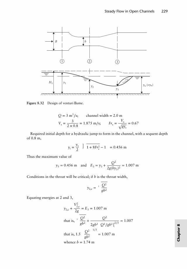
Steady Flow in Open Channels 229
bB
21 3
H1 y1y2
y3
ys (=yn)
Figure 8.32 Design of venturi flume.
Q = 3 m3∕s; channel width = 2.0 m
Vs =3
2 × 0.8= 1.875 m∕s; Frs =
Vs√gys
= 0.67
Required initial depth for a hydraulic jump to form in the channel, with a sequent depthof 0.8 m,
yi =ys
2
(√1 + 8Fr2
s − 1)
= 0.456 m
Thus the maximum value of
y3 = 0.456 m and E3 = y3 +Q2
2g(by3)2= 1.007 m
Conditions in the throat will be critical; if b is the throat width,
y2,c =3
√Q2
gb2
Equating energies at 2 and 3,
y2,c +V2
2,c
2g= E3 = 1.007 m
that is, 3
√Q2
gb2+
Q2
2gb2(Q2∕gb2
)2∕3= 1.007
that is, 1.5(
Q2
gb2
)1∕3
= 1.007 m
whence b = 1.74 m Ch
apte
r8
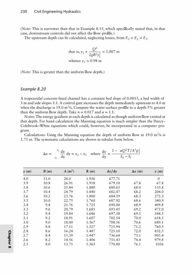
230 Civil Engineering Hydraulics
(Note: This is narrower than that in Example 8.15, which specifically stated that, in thatcase, downstream controls did not affect the flow profile.)
The upstream depth can be calculated, neglecting losses, from E1 = E2 = E3.
that is, y1 +Q2
2gB2y21
= 1.007 m
whence y1 = 0.98 m
(Note: This is greater than the uniform flow depth.)
Example 8.20
A trapezoidal concrete-lined channel has a constant bed slope of 0.0015, a bed width of3 m and side slopes 1:1. A control gate increases the depth immediately upstream to 4.0 mwhen the discharge is 19.0 m3/s. Compute the water surface profile to a depth 5% greaterthan the uniform flow depth. Take n = 0.017 and 𝛼 = 1.1.
Notes: The energy gradient at each depth is calculated as though uniform flow existed atthat depth. For hand calculation the Manning equation is much simpler than the Darcy–Colebrook–White equations which could, however, be incorporated in a computer pro-gram.
Calculations: Using the Manning equation the depth of uniform flow at 19.0 m3/s is1.75 m. The systematic calculations are shown in tabular form below.
Δx = ∫y2
y1
dxdy
dy = x2 − x1 where dxdy
=1 −
(𝛼Q2T∕A3g
)S0 − Sf
y (m) B (m) A (m2) R (m) dx∕dy 𝚫x (m) x (m)
4.0 11.0 28.0 1.956 677.71 03.9 10.8 26.91 1.918 679.10 67.8 67.83.8 10.6 25.84 1.880 680.65 68.0 135.83.7 10.4 24.79 1.840 682.47 68.2 204.03.6 10.2 23.76 1.800 684.59 68.3 272.33.5 10.0 22.75 1.760 687.92 68.6 340.93.4 9.8 21.76 1.725 690.00 68.9 409.83.3 9.6 20.79 1.685 693.45 69.2 472.03.2 9.4 19.84 1.646 697.58 69.5 548.53.1 9.2 18.91 1.607 702.54 70.0 618.53.0 9.0 18.00 1.567 708.56 70.6 689.12.9 8.8 17.11 1.527 715.94 71.2 760.32.8 8.6 16.24 1.487 725.10 72.0 832.32.7 8.4 15.39 1.447 736.64 73.1 905.42.6 8.2 14.56 1.406 751.43 74.4 979.82.5 8.0 13.75 1.365 770.80 76.1 1056
Ch
apter
8
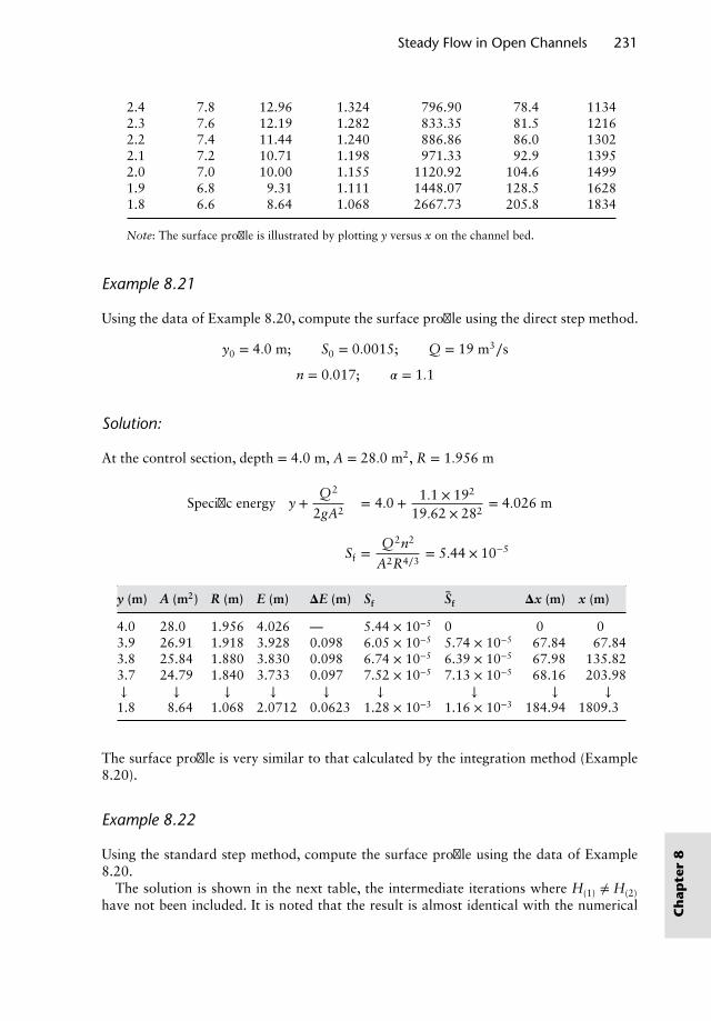
Steady Flow in Open Channels 231
2.4 7.8 12.96 1.324 796.90 78.4 11342.3 7.6 12.19 1.282 833.35 81.5 12162.2 7.4 11.44 1.240 886.86 86.0 13022.1 7.2 10.71 1.198 971.33 92.9 13952.0 7.0 10.00 1.155 1120.92 104.6 14991.9 6.8 9.31 1.111 1448.07 128.5 16281.8 6.6 8.64 1.068 2667.73 205.8 1834
Note: The surface profile is illustrated by plotting y versus x on the channel bed.
Example 8.21
Using the data of Example 8.20, compute the surface profile using the direct step method.
y0 = 4.0 m; S0 = 0.0015; Q = 19 m3∕s
n = 0.017; 𝛼 = 1.1
Solution:
At the control section, depth = 4.0 m, A = 28.0 m2, R = 1.956 m
Specific energy(
y +Q2
2gA2
)= 4.0 + 1.1 × 192
19.62 × 282= 4.026 m
Sf =Q2n2
A2R4∕3= 5.44 × 10⁻⁵
y (m) A (m2) R (m) E (m) 𝚫E (m) Sf Sf 𝚫x (m) x (m)
4.0 28.0 1.956 4.026 — 5.44 × 10⁻⁵ 0 0 03.9 26.91 1.918 3.928 0.098 6.05 × 10⁻⁵ 5.74 × 10⁻⁵ 67.84 67.843.8 25.84 1.880 3.830 0.098 6.74 × 10⁻⁵ 6.39 × 10⁻⁵ 67.98 135.823.7 24.79 1.840 3.733 0.097 7.52 × 10⁻⁵ 7.13 × 10⁻⁵ 68.16 203.98↓ ↓ ↓ ↓ ↓ ↓ ↓ ↓ ↓
1.8 8.64 1.068 2.0712 0.0623 1.28 × 10⁻³ 1.16 × 10⁻³ 184.94 1809.3
The surface profile is very similar to that calculated by the integration method (Example8.20).
Example 8.22
Using the standard step method, compute the surface profile using the data of Example8.20.
The solution is shown in the next table, the intermediate iterations where H(1) ≠ H(2)have not been included. It is noted that the result is almost identical with the numerical C
hap
ter
8
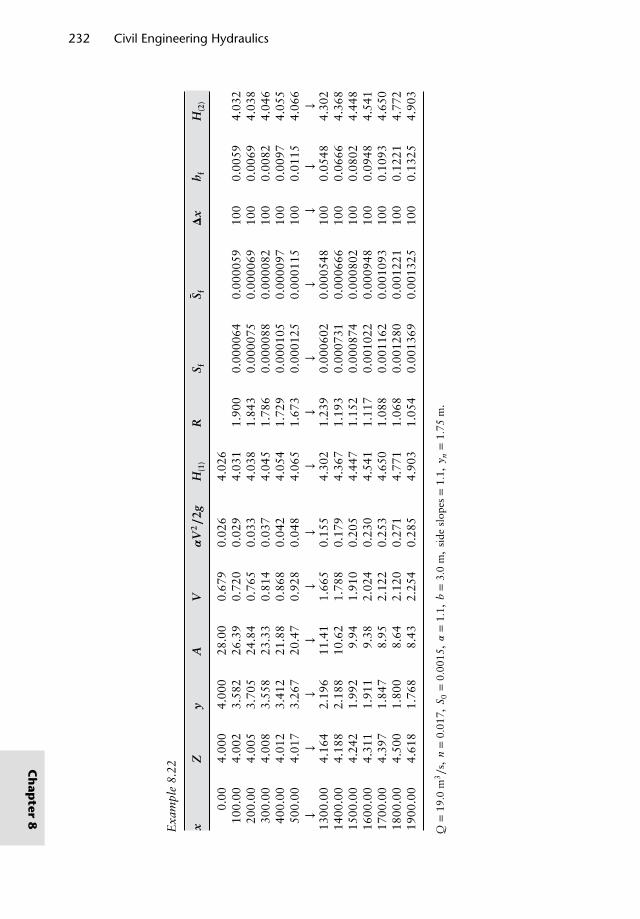
232 Civil Engineering Hydraulics
Exa
mpl
e8.
22
xZ
yA
V𝜶
V2∕2
gH
(1)
RS f
S f𝚫x
h fH
(2)
0.00
4.00
04.
000
28.0
00.
679
0.02
64.
026
100.
004.
002
3.58
226
.39
0.72
00.
029
4.03
11.
900
0.00
0064
0.00
0059
100
0.00
594.
032
200.
004.
005
3.70
524
.84
0.76
50.
033
4.03
81.
843
0.00
0075
0.00
0069
100
0.00
694.
038
300.
004.
008
3.55
823
.33
0.81
40.
037
4.04
51.
786
0.00
0088
0.00
0082
100
0.00
824.
046
400.
004.
012
3.41
221
.88
0.86
80.
042
4.05
41.
729
0.00
0105
0.00
0097
100
0.00
974.
055
500.
004.
017
3.26
720
.47
0.92
80.
048
4.06
51.
673
0.00
0125
0.00
0115
100
0.01
154.
066
↓↓
↓↓
↓↓
↓↓
↓↓
↓↓
↓13
00.0
04.
164
2.19
611
.41
1.66
50.
155
4.30
21.
239
0.00
0602
0.00
0548
100
0.05
484.
302
1400
.00
4.18
82.
188
10.6
21.
788
0.17
94.
367
1.19
30.
0007
310.
0006
6610
00.
0666
4.36
815
00.0
04.
242
1.99
29.
941.
910
0.20
54.
447
1.15
20.
0008
740.
0008
0210
00.
0802
4.44
816
00.0
04.
311
1.91
19.
382.
024
0.23
04.
541
1.11
70.
0010
220.
0009
4810
00.
0948
4.54
117
00.0
04.
397
1.84
78.
952.
122
0.25
34.
650
1.08
80.
0011
620.
0010
9310
00.
1093
4.65
018
00.0
04.
500
1.80
08.
642.
120
0.27
14.
771
1.06
80.
0012
800.
0012
2110
00.
1221
4.77
219
00.0
04.
618
1.76
88.
432.
254
0.28
54.
903
1.05
40.
0013
690.
0013
2510
00.
1325
4.90
3
Q=
19.0
m3∕s
,n=
0.01
7,S 0
=0.
0015
,𝛼=
1.1,
b=
3.0
m,
side
slop
es=
1.1,
y n=
1.75
m.
Ch
apter
8
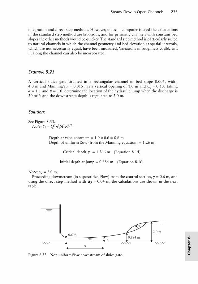
Steady Flow in Open Channels 233
integration and direct step methods. However, unless a computer is used the calculationsin the standard step method are laborious, and for prismatic channels with constant bedslopes the other methods would be quicker. The standard step method is particularly suitedto natural channels in which the channel geometry and bed elevation at spatial intervals,which are not necessarily equal, have been measured. Variations in roughness coefficient,n, along the channel can also be incorporated.
Example 8.23
A vertical sluice gate situated in a rectangular channel of bed slope 0.005, width4.0 m and Manning’s n = 0.015 has a vertical opening of 1.0 m and Cc = 0.60. Taking𝛼 = 1.1 and 𝛽 = 1.0, determine the location of the hydraulic jump when the discharge is20 m3/s and the downstream depth is regulated to 2.0 m.
Solution:
See Figure 8.33.Note: Sf = Q2n2∕A2R4∕3.
Depth at vena contracta = 1.0 × 0.6 = 0.6 mDepth of uniform flow (from the Manning equation) = 1.26 m
Critical depth, yc = 1.366 m (Equation 8.14)
Initial depth at jump = 0.884 m (Equation 8.16)
Note: ys = 2.0 m.Proceeding downstream (in supercritical flow) from the control section, y = 0.6 m, and
using the direct step method with Δy = 0.04 m, the calculations are shown in the nexttable.
0.6 m0.884 m
2.0 m
x
y
Figure 8.33 Non-uniform flow downstream of sluice gate. Ch
apte
r8
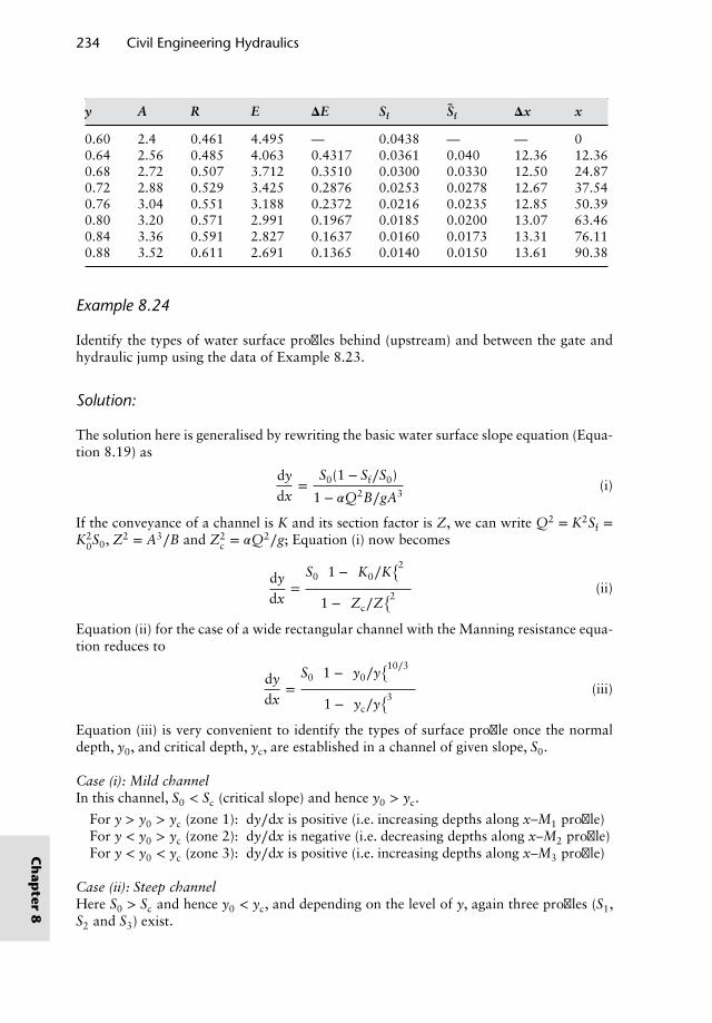
234 Civil Engineering Hydraulics
y A R E 𝚫E Sf Sf 𝚫x x
0.60 2.4 0.461 4.495 — 0.0438 — — 00.64 2.56 0.485 4.063 0.4317 0.0361 0.040 12.36 12.360.68 2.72 0.507 3.712 0.3510 0.0300 0.0330 12.50 24.870.72 2.88 0.529 3.425 0.2876 0.0253 0.0278 12.67 37.540.76 3.04 0.551 3.188 0.2372 0.0216 0.0235 12.85 50.390.80 3.20 0.571 2.991 0.1967 0.0185 0.0200 13.07 63.460.84 3.36 0.591 2.827 0.1637 0.0160 0.0173 13.31 76.110.88 3.52 0.611 2.691 0.1365 0.0140 0.0150 13.61 90.38
Example 8.24
Identify the types of water surface profiles behind (upstream) and between the gate andhydraulic jump using the data of Example 8.23.
Solution:
The solution here is generalised by rewriting the basic water surface slope equation (Equa-tion 8.19) as
dy
dx=
S0(1 − Sf∕S0)
1 − 𝛼Q2B∕gA3(i)
If the conveyance of a channel is K and its section factor is Z, we can write Q2 = K2Sf =K2
0S0, Z2 = A3∕B and Z2c = 𝛼Q2∕g; Equation (i) now becomes
dy
dx=
S0
[1 −
(K0∕K
)2]
1 −(Zc∕Z
)2(ii)
Equation (ii) for the case of a wide rectangular channel with the Manning resistance equa-tion reduces to
dy
dx=
S0
[1 −
(y0∕y
)10∕3]
1 −(yc∕y
)3(iii)
Equation (iii) is very convenient to identify the types of surface profile once the normaldepth, y0, and critical depth, yc, are established in a channel of given slope, S0.
Case (i): Mild channelIn this channel, S0 < Sc (critical slope) and hence y0 > yc.
For y > y0 > yc (zone 1): dy∕dx is positive (i.e. increasing depths along x–M1 profile)For y < y0 > yc (zone 2): dy∕dx is negative (i.e. decreasing depths along x–M2 profile)For y < y0 < yc (zone 3): dy∕dx is positive (i.e. increasing depths along x–M3 profile)
Case (ii): Steep channelHere S0 > Sc and hence y0 < yc, and depending on the level of y, again three profiles (S1,S2 and S3) exist.
Ch
apter
8
Steady Flow in Open Channels 235
Case (iii): Critical slope channelHere S0 = Sc and y0 = yc; zone 2 is absent, and two profiles (C1 and C3) exist.
Case (iv): Horizontal channelHere S0 = 0 and y0 will not exist and hence zone 1 is absent; again two profiles (H2 andH3) exist.
Case (v): Adverse slope channelNow S0 is negative with no y0 and two profiles (A2 and A3) exist in this case. The dis-charge Q = 20 m3/s and by the Manning resistance equation y0 = 1.26 m. The criticaldepth in rectangular channel yc = (𝛼Q2∕b2g)1∕3. Hence yc = 1.366 m > y0; hence, steepchannel with gate opening below critical depth. The depth upstream of the gate (by energybalance)= 4.05 m> yc > y0; zone 1 is on steep slope; S1 profile exists immediately upstreamof the gate.
The flow downstream of the gate is supercritical (zone 3 of the steep channel) mergingwith the controlled subcritical flow with the formation of hydraulic jump. Here the S3profile forms between the depths, 0.6 m (just d∕s of gate) and 0.884 m, sequential to thecontrolled depth of 2 m.
Example 8.25
Discharge from a natural lake occurs through a very long rectangular channel of bed width3 m, Manning’s n = 0.014 and the bed slope = 0.001. The maximum level of the watersurface in the lake above the channel bed at the lake outlet is 3 m. Calculate the discharge inthe channel. If the channel slope were to be 0.008, compute the discharge. Also, determinethe uniform flow depth and the minimum length of the channel for the uniform flow toestablish. Ignore entrance losses.
Solution:
Slope = 0.001; first establish whether this is a mild or steep slope. If the slope were to beassumed critical, the channel will have inlet control with critical depth; critical depth ina rectangular channel is 2H/3, H being the energy head (lake level above channel inlet)available.
Therefore the critical depth at inlet, yc =23× 3 = 2 m
Since the channel is long (with no downstream control), uniform flow with depth y0 = ycestablishes at the inlet itself; using the Manning resistance equation, the correspondingcritical slope, Sc, is computed.
At critical depth the discharge is maximum and is computed from yc = (q2∕g)1∕3 (from𝛼Q2B∕gA3 = 1). Hence, Q = qb = 26.58 m3/s, and from Q = An−1R2∕3S1∕2 the slope, S =Sc = 0.0047.
If the channel is other than rectangular in cross section, two simultaneous equations(i) the energy equation and (ii) the critical depth criterion, 𝛼Q2B∕gA3 = 1, must be solvedfor computing yc.
Since the bed slope S0 < Sc, the channel is of mild slope. Ch
apte
r8
236 Civil Engineering Hydraulics
Two equations at the inlet to solve two unknowns, depth and velocity, are required:
(i) Energy equation, H = y0 + V2∕2g(ii) The Manning resistance equation, V = n−1R2∕3S1∕2
Both are applicable at the inlet (long channel; uniform flow establishes from the inlet).Simultaneous solution of (i) and (ii) gives
y0 = 2.75 m and V = 2.213 m∕sThus the discharge, Q0 = 18.26 m3∕s
The slope S0 = 0.008 > Sc = 0.0047; the channel is a steep-sloped one, and the inlet con-trols the flow. The discharge is maximum (= 26.58m3∕s) with critical depth at the inlet(yc = 2 m). The corresponding uniform flow depth (y0) from the Manning resistance equa-tion
26.58 × 3 × y0 × (1∕0.014) × [(3 × y0)∕(3 + 2y0)]2∕3 × (0.008)1∕2
is computed. Thus y0 = 1.64 m; this unform flow establishes in the channel if its length isat least equal to the length of the surface profile (non-uniform flow) that exists betweenthe inlet depth, yc, and the uniform flow depth, y0.
The channel is of steep slope, and the flow between these two depths corresponds toregion 2 and hence an S2 profile develops whose length can be computed by any appro-priate method. By the step method we obtain L ≈ 80 m between the two depths; the cal-culations should commence at a depth slightly less than the critical depth and terminateat a depth slightly higher than the normal (uniform) depth.
Example 8.26
A rectangular channel (b = 15 m, length = 10 km, slope = 1/10 000, Manning’s n = 0.015)fed by an upstream lake is discharging into a downstream lake. If the upstream and down-stream lake levels are 1.5 and 2 m (above the channel bed), respectively, determine thedischarge rate in the channel.
Solution:
The channel delivery depends upon the following considerations:
(i) Is the channel long (i.e. no downstream control)?(ii) Is the slope mild or critical or steep?
If we assume a long and mild channel, two equations at its inlet are applicable (i.e. theenergy and resistance equations). If we assume a long and critical sloped channel, the twoequations are the energy equation and the critical depth criterion. Here it is convenientto assume initially a long and critical sloped channel. Since the channel is of rectangularcross section, yc = 2H∕3 = 1 m. Therefore, from the Manning resistance equation (uni-form flow depth = yc), the critical slope, Sc = 0.00256 > S0 = 0.0001 (see Example 8.25).Hence the channel is of mild slope; if we still assume that it is long, we now can obtainthe corresponding uniform flow rate, Q0, from the energy and resistance equations.
(iii) Is the channel long enough to satisfy the above assumptions?
Ch
apter
8
Steady Flow in Open Channels 237
Identify the type of water surface profile based on the discharge, uniform flow depth anddownstream lake level and compute its length. If the surface profile length is shorter thanchannel length, the channel is long enough and uniform flow does exist at the inlet (i.e.free inlet). If the profile length is longer than the channel length, the inlet will be drowned(short channel) and the discharge rate is reduced. To compute the actual discharge rate ina short channel, the following iterative procedure is to be followed:
(a) Assume Q < Q0 (since the inlet is drowned) and compute the corresponding flowdepth at the inlet by the energy equation.
(b) Compute the new surface profile length corresponding to this discharge and verifywhether it fits between the inlet depth and the downstream lake level.
(c) Repeat (a) and (b) until the profile length matches the channel length.
The problem is best approached on a computer for executing these iterative procedures.
Example 8.27
A concrete twin-box-type culvert is proposed to discharge a design flood of 13.5 m3/s. Thefollowing data refer to each opening:
Manning’s n = 0.013Height = 0.75 mWidth = 1.5 mLength = 30 mSlope = 1/100Entrance conditions = square edge, loss coefficient, K = 0.5Downstream conditions = free jet
Establish the rating curve (discharge vs. headwater elevation above the invert at theentrance) for rising head conditions over a discharge range from 0 to 13.5 m3/s. Neglectthe velocity of approach. Determine the minimum elevation of the road surface assuminga free board of 300 mm to avoid any flooding of the highway.
Solution:
The culvert behaviour is dependent on the headwater level H, the height of culvert D, slopeSo and length L; here the outlet is to discharge freely and has no effect on the type of flowthrough the culvert.
(i) For H∕D ≤ 1.2, open channel flow. If entrance control exists, the depth at the inletis critical (i.e. the slope is either critical or steep). Assuming entrance control, yc =(2∕3) × H (rectangular channel; inlet with no entrance losses) and Vc =
√gyc; hence,
Q can be computed. Also from the Manning resistance equation, the critical slope, Sc,can be computed and checked against the proposed slope of the culvert; if the slopeis then found to be mild, the depth and discharge calculations must be computed bythe energy and resistance equations (see Example 8.25).
The energy equation at the inlet gives H = 1.75yc, assuming entrance control witha loss coefficient of 0.5 (i.e. S0 ≥ Sc).
Ch
apte
r8
238 Civil Engineering Hydraulics
For H = 0.1 m, yc = 0.057 m and Vc = 0.748 m/s. From the Manning equation,Sc = 0.00476, and as S0 (= 0.01) > Sc (= 0.00476), entrance control exists. The dis-charge through the culvert of width b can be written as Q = byc
√gyc for one box.
Various values for yc and hence the headwater levels (H = 1.75yc) are assumed untilH = 1.2D (=0.9 m, the upper limit for open channel flow); a check for S0 > Sc isnecessary for all values.
Headwater level H (m) Discharge Q (m3/s) (two boxes)
0.175 0.2970.525 1.5440.700 2.3770.900 3.465
(ii) For H∕D ≥ 1.2, the culvert entry behaves like an orifice (constriction); if the normaldepth in the barrel corresponding to the orifice discharge is less than D, the flowdownstream of the inlet is free. The orifice flow equation
Q = Cd × b × D ×[2g
(H − D
2
)]1∕2for one box
with the discharge coefficient Cd = 0.62 (assumed). Computations between H =1.2D and the value at which y0 = D are as below:
Headwater level H (m) Discharge Q (m3/s) (two boxes)
0.900 4.4771.300 5.9431.700 7.1132.100 8.1162.500 9.007
(iii) For H∕D > 1.2 and y0 > D, pipe flow exists in the culvert. The energy equationbetween the inlet and outlet of the culvert gives
H + S0L = D + (1 + K)V2
2g+ SfL
where Sf is the friction slope given by the Manning equation, as Sf = (Vn)2∕R4∕3. Theabove reduce to
Q = 3.41(H − 0.45)1∕2 for one box
pipe flow condition with the following:
Ch
apter
8
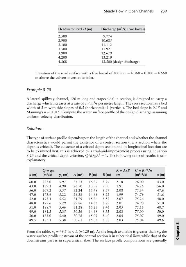
Steady Flow in Open Channels 239
Headwater level H (m) Discharge (m3/s) (two boxes)
2.500 9.7742.900 10.6853.100 11.1123.500 11.9213.900 12.6794.200 13.2194.368 13.500 (design discharge)
Elevation of the road surface with a free board of 300 mm = 4.368 + 0.300 = 4.668m above the culvert invert at its inlet.
Example 8.28
A lateral spillway channel, 120 m long and trapezoidal in section, is designed to carry adischarge which increases at a rate of 3.7 m3/s per metre length. The cross section has a bedwidth of 3 m with side slopes of 0.5 (horizontal) : 1 (vertical). The bed slope is 0.15 andManning’s n = 0.015. Compute the water surface profile of the design discharge assuminguniform velocity distribution.
Solution:
The type of surface profile depends upon the length of the channel and whether the channelcharacteristics would permit the existence of a control section (i.e. a section where thedepth is critical). The existence of a critical depth section and its longitudinal location areto be examined first; this is achieved by a trial-and-improvement process using Equation8.23 and the critical depth criterion, Q2B∕gA3 = 1. The following table of results is self-explanatory:
Q = qx R = A∕P C = R1∕6/nx (m) (m3/s) yc (m) A (m2) P (m) B (m) (m) (m1∕2/s) x (m)
60.0 222.0 5.97 35.73 16.37 8.97 2.18 76.00 43.043.0 159.1 4.90 26.70 13.98 7.90 1.91 74.26 56.056.0 207.2 5.57 32.24 15.48 8.57 2.08 75.34 47.647.0 173.9 5.22 29.28 14.69 8.22 1.99 74.79 51.652.0 192.4 5.52 31.79 15.36 8.52 2.07 75.26 48.048.0 177.6 5.29 29.86 14.85 8.29 2.01 74.90 51.051.0 188.7 5.46 31.28 15.23 8.46 2.05 75.16 48.749.0 181.3 5.35 30.36 14.98 8.35 2.03 75.00 50.050.0 185.0 5.40 30.78 15.09 8.40 2.04 75.07 49.049.5 183.1 5.38 30.61 15.05 8.38 2.03 75.04 49.6
From the table, xc = 49.5 m < L (=120 m). As the length available is greater than xc, thewater surface profile upstream of the control section is in subcritical flow, while that of thedownstream part is in supercritical flow. The surface profile computations are generally C
hap
ter
8
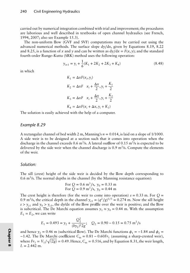
240 Civil Engineering Hydraulics
carried out by numerical integration combined with trial and improvement; the proceduresare laborious and well described in textbooks of open channel hydraulics (see French,1994, 2007; also see Example 15.3).
The non-uniform flow (GVF and SVF) computations may be carried out using theadvanced numerical methods. The surface slope dy∕dx, given by Equations 8.19, 8.22and 8.25, is a function of x and y and can be written as dy∕dx = F(x, y); and the standardfourth-order Runge–Kutta (SRK) method uses the following operation:
yi+1 = yi +16
(K1 + 2K2 + 2K3 + K4) (8.48)
in which
K1 = ΔxF(xi, yi)
K2 = ΔxF(
xi +Δx2
, yi +K1
2
)
K3 = ΔxF(
xi +Δx2
, yi +K2
2
)K4 = ΔxF(xi + Δx, yi + K3)
The solution is easily achieved with the help of a computer.
Example 8.29
A rectangular channel of bed width 2 m, Manning’s n = 0.014, is laid on a slope of 1/1000.A side weir is to be designed at a section such that it comes into operation when thedischarge in the channel exceeds 0.6 m3/s. A lateral outflow of 0.15 m3/s is expected to bedelivered by the side weir when the channel discharge is 0.9 m3/s. Compute the elementsof the weir.
Solution:
The sill (crest) height of the side weir is decided by the flow depth corresponding to0.6 m3/s. The normal depths in the channel (by the Manning resistance equation):
For Q = 0.6 m3∕s, y0 = 0.33 mFor Q = 0.9 m3∕s, y0 = 0.44 m
The crest height is therefore (for the weir to come into operation) s = 0.33 m. For Q =0.9 m3/s, the critical depth in the channel yc1 = (q2∕g)1∕3 = 0.274 m. Now the sill heights > yc1 and y0 > yc1, the dy/dx of the flow profile over the weir is positive; and the flowis subcritical. The De Marchi equation assumes y1 ≈ y0 = 0.44 m. With the assumptionE1 = E2, we can write
E1 = 0.493 = y2 +Q2
2
(by2)22g; Q2 = 0.90 − 0.15 = 0.75 m3∕s
and hence y2 = 0.46 m (subcritical flow). The De Marchi functions 𝜙1 = −1.84 and 𝜙2 =−1.42. The De Marchi coefficient Cm = 0.81 − 0.60Fr1 (assuming a sharp-crested weir),where Fr1 = V1∕
√(2g) = 0.49. Hence, Cm = 0.516, and by Equation 8.31, the weir length,
L = 2.442 m.
Ch
apter
8
Steady Flow in Open Channels 241
References and recommended reading
Ackers, P. (1992) Hydraulic design of two-stage channels. Proceedings of the Institution ofCivil Engineers, Water, Maritime & Energy, 96, 247–257, and discussion in March 1994,106, 99–101.
Balkham, M., Fosbeary, C., Kitchen, A. and Rickard, C. (2010) Culvert Design and OperationGuide, C689, CIRIA, London.
British Standards Institution (1981) Methods of Measurement of Liquid Flow in Open Chan-nels – Thin Plate Weirs, BS 3680, Part 4A, British Standards Institution, London.
British Standards Institution (1981) Methods of Measurement of Liquid Flow in Open Chan-nels – Flumes, BS 3680, Part 4C, British Standards Institution, London.
Chadwick, A., Morfett, J. and Borthwick, M. (2013) Hydraulics in Civil and EnvironmentalEngineering, 5th edn, Taylor & Francis, Abingdon, UK.
Chanson, H. (2004) The Hydraulics of Open Channel Flow, 2nd edn, Elsevier Butterworth-Heinemann, Oxford.
Chow, V. T. (1959) Open-Channel Hydraulics, McGraw-Hill, New York.Fortier, S. and Scobey, F. C. (1926) Permissible canal velocities. Transactions of the American
Society of Civil Engineers, 89, 940–984.French, R. H. (1994) Open Channel Hydraulics, 2nd edn, McGraw-Hill, New York.French, R. H. (2007) Open Channel Hydraulics, Water Resources Publications, Highlands
Ranch, CO.Henderson, F. M. (1966) Open Channel Flow, Macmillan, New York.HR Wallingford (1990) Charts for the Hydraulic Design of Channels and Pipes, 6th edn,
Thomas Telford, London.HR Wallingford (1990) Tables for the Hydraulic Design of Pipes and Sewers, 5th edn, Thomas
Telford, London.HR Wallingford and Barr, D. I. H. (2006) Tables for the Hydraulic Design of Pipes, Sewers and
Channels, 8th edn, Thomas Telford, London.Mansell, M. G. (2003) Rural and Urban Hydrology, Thomas Telford, London.National Water Council (1981) Design and Analysis of Urban Storm Drainage, the Walling-
ford Procedure, Volume 4: The Modified Rational Method, National Water Council StandingTechnical Committee Report No. 31, National Water Council, London.
Novak, P., Moffat, A. I. B., Nalluri, C. and Narayanan, R. (2007) Hydraulic Structures, 4th edn,Taylor & Francis, Abingdon, UK.
Ramsbottom, D., Day, R. and Rickard, C. (1997) Culvert Design Mannual, Report 168, CIRIA,London.
Water UK/WRc (2012) Sewers for Adoption – A Design and Construction Guide for Develop-ers, 7th edn, WRc, Swindon.
Problems
1. Water flows uniformly at a depth of 2 m in a rectangular channel of width 4 m and bedslope 1:2000. What is the mean shear stress on the wetted perimeter?
2. (a) At a measured discharge of 40 m3/s, the depth of uniform flow in a rectangularchannel 5 m wide and with a bed slope of 1:1000 was 3.05 m. Determine the meaneffective roughness size and the Manning roughness coefficient.
(b) Using (i) the Darcy–Weisbach equation (together with the Colebrook–White equa-tion) and (ii) the Manning equation, predict the discharge at a depth of 4 m. C
hap
ter
8
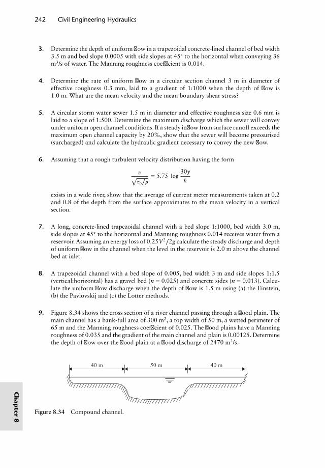
242 Civil Engineering Hydraulics
3. Determine the depth of uniform flow in a trapezoidal concrete-lined channel of bed width3.5 m and bed slope 0.0005 with side slopes at 45◦ to the horizontal when conveying 36m3/s of water. The Manning roughness coefficient is 0.014.
4. Determine the rate of uniform flow in a circular section channel 3 m in diameter ofeffective roughness 0.3 mm, laid to a gradient of 1:1000 when the depth of flow is1.0 m. What are the mean velocity and the mean boundary shear stress?
5. A circular storm water sewer 1.5 m in diameter and effective roughness size 0.6 mm islaid to a slope of 1:500. Determine the maximum discharge which the sewer will conveyunder uniform open channel conditions. If a steady inflow from surface runoff exceeds themaximum open channel capacity by 20%, show that the sewer will become pressurised(surcharged) and calculate the hydraulic gradient necessary to convey the new flow.
6. Assuming that a rough turbulent velocity distribution having the form
v√𝜏0∕𝜌
= 5.75 log30y
k
exists in a wide river, show that the average of current meter measurements taken at 0.2and 0.8 of the depth from the surface approximates to the mean velocity in a verticalsection.
7. A long, concrete-lined trapezoidal channel with a bed slope 1:1000, bed width 3.0 m,side slopes at 45◦ to the horizontal and Manning roughness 0.014 receives water from areservoir. Assuming an energy loss of 0.25V2∕2g calculate the steady discharge and depthof uniform flow in the channel when the level in the reservoir is 2.0 m above the channelbed at inlet.
8. A trapezoidal channel with a bed slope of 0.005, bed width 3 m and side slopes 1:1.5(vertical:horizontal) has a gravel bed (n = 0.025) and concrete sides (n = 0.013). Calcu-late the uniform flow discharge when the depth of flow is 1.5 m using (a) the Einstein,(b) the Pavlovskij and (c) the Lotter methods.
9. Figure 8.34 shows the cross section of a river channel passing through a flood plain. Themain channel has a bank-full area of 300 m2, a top width of 50 m, a wetted perimeter of65 m and the Manning roughness coefficient of 0.025. The flood plains have a Manningroughness of 0.035 and the gradient of the main channel and plain is 0.00125. Determinethe depth of flow over the flood plain at a flood discharge of 2470 m3/s.
m40m40 50 m
Figure 8.34 Compound channel.
Ch
apter
8
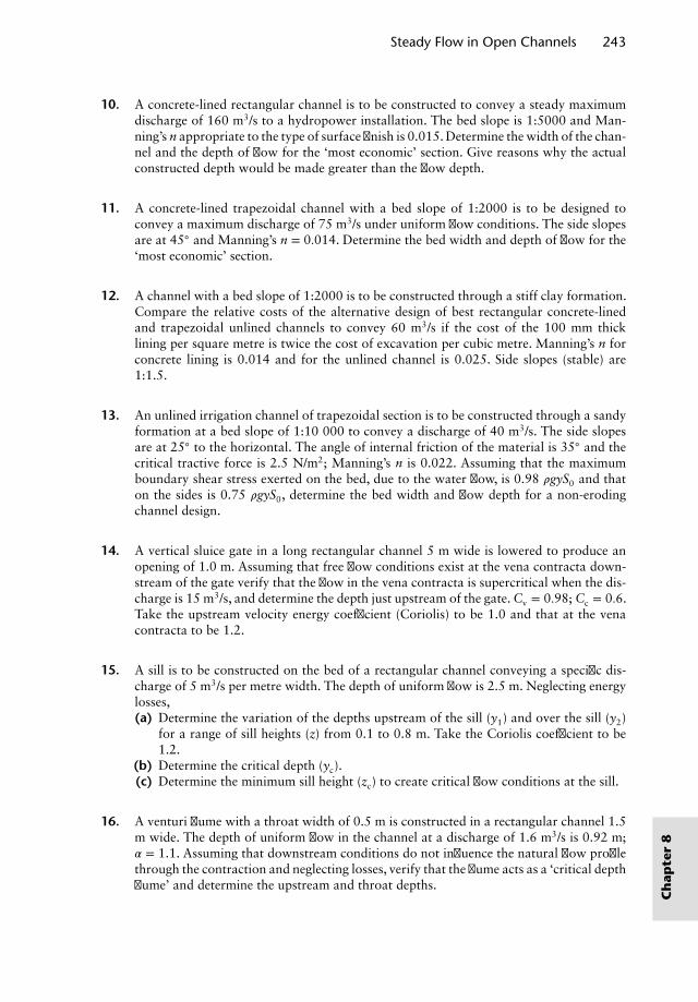
Steady Flow in Open Channels 243
10. A concrete-lined rectangular channel is to be constructed to convey a steady maximumdischarge of 160 m3/s to a hydropower installation. The bed slope is 1:5000 and Man-ning’s n appropriate to the type of surface finish is 0.015. Determine the width of the chan-nel and the depth of flow for the ‘most economic’ section. Give reasons why the actualconstructed depth would be made greater than the flow depth.
11. A concrete-lined trapezoidal channel with a bed slope of 1:2000 is to be designed toconvey a maximum discharge of 75 m3/s under uniform flow conditions. The side slopesare at 45◦ and Manning’s n = 0.014. Determine the bed width and depth of flow for the‘most economic’ section.
12. A channel with a bed slope of 1:2000 is to be constructed through a stiff clay formation.Compare the relative costs of the alternative design of best rectangular concrete-linedand trapezoidal unlined channels to convey 60 m3/s if the cost of the 100 mm thicklining per square metre is twice the cost of excavation per cubic metre. Manning’s n forconcrete lining is 0.014 and for the unlined channel is 0.025. Side slopes (stable) are1:1.5.
13. An unlined irrigation channel of trapezoidal section is to be constructed through a sandyformation at a bed slope of 1:10 000 to convey a discharge of 40 m3/s. The side slopesare at 25◦ to the horizontal. The angle of internal friction of the material is 35◦ and thecritical tractive force is 2.5 N/m2; Manning’s n is 0.022. Assuming that the maximumboundary shear stress exerted on the bed, due to the water flow, is 0.98 𝜌gyS0 and thaton the sides is 0.75 𝜌gyS0, determine the bed width and flow depth for a non-erodingchannel design.
14. A vertical sluice gate in a long rectangular channel 5 m wide is lowered to produce anopening of 1.0 m. Assuming that free flow conditions exist at the vena contracta down-stream of the gate verify that the flow in the vena contracta is supercritical when the dis-charge is 15 m3/s, and determine the depth just upstream of the gate. Cv = 0.98; Cc = 0.6.Take the upstream velocity energy coefficient (Coriolis) to be 1.0 and that at the venacontracta to be 1.2.
15. A sill is to be constructed on the bed of a rectangular channel conveying a specific dis-charge of 5 m3/s per metre width. The depth of uniform flow is 2.5 m. Neglecting energylosses,(a) Determine the variation of the depths upstream of the sill (y1) and over the sill (y2)
for a range of sill heights (z) from 0.1 to 0.8 m. Take the Coriolis coefficient to be1.2.
(b) Determine the critical depth (yc).(c) Determine the minimum sill height (zc) to create critical flow conditions at the sill.
16. A venturi flume with a throat width of 0.5 m is constructed in a rectangular channel 1.5m wide. The depth of uniform flow in the channel at a discharge of 1.6 m3/s is 0.92 m;𝛼 = 1.1. Assuming that downstream conditions do not influence the natural flow profilethrough the contraction and neglecting losses, verify that the flume acts as a ‘critical depthflume’ and determine the upstream and throat depths.
Ch
apte
r8
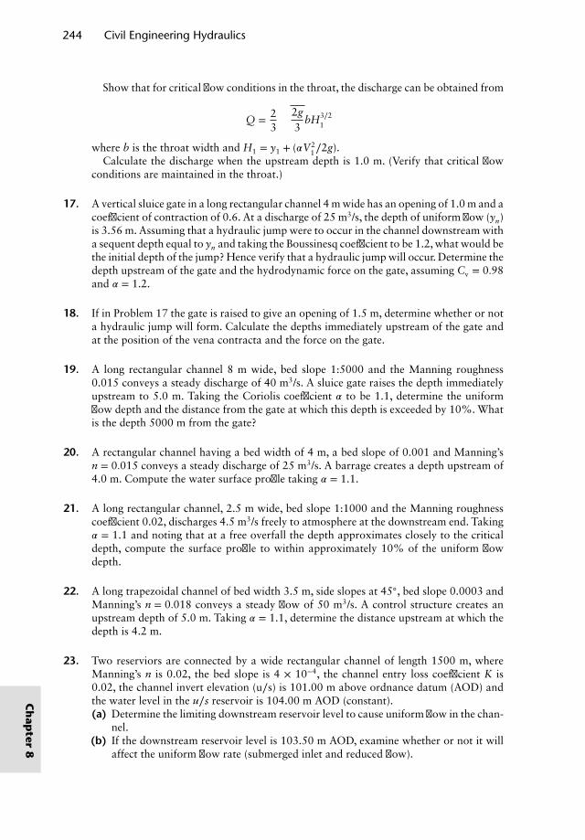
244 Civil Engineering Hydraulics
Show that for critical flow conditions in the throat, the discharge can be obtained from
Q = 23
√2g3
bH3∕21
where b is the throat width and H1 = y1 + (𝛼V21∕2g).
Calculate the discharge when the upstream depth is 1.0 m. (Verify that critical flowconditions are maintained in the throat.)
17. A vertical sluice gate in a long rectangular channel 4 m wide has an opening of 1.0 m and acoefficient of contraction of 0.6. At a discharge of 25 m3/s, the depth of uniform flow (yn)is 3.56 m. Assuming that a hydraulic jump were to occur in the channel downstream witha sequent depth equal to yn and taking the Boussinesq coefficient to be 1.2, what would bethe initial depth of the jump? Hence verify that a hydraulic jump will occur. Determine thedepth upstream of the gate and the hydrodynamic force on the gate, assuming Cv = 0.98and 𝛼 = 1.2.
18. If in Problem 17 the gate is raised to give an opening of 1.5 m, determine whether or nota hydraulic jump will form. Calculate the depths immediately upstream of the gate andat the position of the vena contracta and the force on the gate.
19. A long rectangular channel 8 m wide, bed slope 1:5000 and the Manning roughness0.015 conveys a steady discharge of 40 m3/s. A sluice gate raises the depth immediatelyupstream to 5.0 m. Taking the Coriolis coefficient 𝛼 to be 1.1, determine the uniformflow depth and the distance from the gate at which this depth is exceeded by 10%. Whatis the depth 5000 m from the gate?
20. A rectangular channel having a bed width of 4 m, a bed slope of 0.001 and Manning’sn = 0.015 conveys a steady discharge of 25 m3/s. A barrage creates a depth upstream of4.0 m. Compute the water surface profile taking 𝛼 = 1.1.
21. A long rectangular channel, 2.5 m wide, bed slope 1:1000 and the Manning roughnesscoefficient 0.02, discharges 4.5 m3/s freely to atmosphere at the downstream end. Taking𝛼 = 1.1 and noting that at a free overfall the depth approximates closely to the criticaldepth, compute the surface profile to within approximately 10% of the uniform flowdepth.
22. A long trapezoidal channel of bed width 3.5 m, side slopes at 45◦, bed slope 0.0003 andManning’s n = 0.018 conveys a steady flow of 50 m3/s. A control structure creates anupstream depth of 5.0 m. Taking 𝛼 = 1.1, determine the distance upstream at which thedepth is 4.2 m.
23. Two reserviors are connected by a wide rectangular channel of length 1500 m, whereManning’s n is 0.02, the bed slope is 4 × 10⁻⁴, the channel entry loss coefficient K is0.02, the channel invert elevation (u∕s) is 101.00 m above ordnance datum (AOD) andthe water level in the u∕s reservoir is 104.00 m AOD (constant).(a) Determine the limiting downstream reservoir level to cause uniform flow in the chan-
nel.(b) If the downstream reservoir level is 103.50 m AOD, examine whether or not it will
affect the uniform flow rate (submerged inlet and reduced flow).
Ch
apter
8
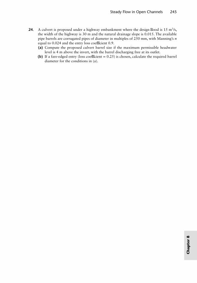
Steady Flow in Open Channels 245
24. A culvert is proposed under a highway embankment where the design flood is 15 m3/s,the width of the highway is 30 m and the natural drainage slope is 0.015. The availablepipe barrels are corrugated pipes of diameter in multiples of 250 mm, with Manning’s nequal to 0.024 and the entry loss coefficient 0.9.(a) Compute the proposed culvert barrel size if the maximum permissible headwater
level is 4 m above the invert, with the barrel discharging free at its outlet.(b) If a fare-edged entry (loss coefficient = 0.25) is chosen, calculate the required barrel
diameter for the conditions in (a).
Ch
apte
r8

Chapter 9Dimensional Analysis,Similitude and HydraulicModels
9.1 Introduction
Hydraulic engineering structures or machines can be designed using (i) pure theory, (ii)empirical methods, (iii) semi-empirical methods, which are mathematical formulationsbased on theoretical concepts supported by suitably designed experiments, (iv) physicalmodels or (v) mathematical models.
The purely theoretical approach in hydraulic engineering is limited to a few cases oflaminar flow, for example the Hagen–Poiseuille equation for the hydraulic gradient inthe laminar flow of an incompressible fluid in a circular pipeline. Empirical methods arebased on correlations between observed variables affecting a particular physical system.Such relationships should only be used under circumstances similar to those under whichthe data were collected. Due to the inability to express the physical interaction of theparameters involved in mathematical terms, some such methods are still in use. One well-known example is in the relationship between wave height, fetch, wind speed and durationfor the forecasting of ocean wave characteristics.
A good example of a semi-empirical relationship is the Colebrook–White equation forthe friction factors in turbulent flow in pipes (see Chapters 4 and 7). This was obtainedfrom theoretical concepts and experiments designed on the basis of dimensional analysis;it is universally applicable to all Newtonian fluids.
Dimensional analysis also forms the basis for the design and operation of physical scalemodels which are used to predict the behaviour of their full-sized counterparts called pro-totypes. Such models, which are generally geometrically similar to the prototype, are usedin the design of aircraft, ships, submarines, pumps, turbines, harbours, breakwaters, riverand estuary engineering works, spillways and so on.
While mathematical modelling techniques have progressed rapidly due to the adventof high-speed digital computers, enabling the equations of motion coupled with semi-empirical relationships to be solved for complex flow situations such as pipe networkanalysis, pressure transients in pipelines and unsteady flows in rivers and estuaries, there
Nalluri & Featherstone’s Civil Engineering Hydraulics: Essential Theory with Worked Examples,Sixth Edition. Martin Marriott.© 2016 John Wiley & Sons, Ltd. Published 2016 by John Wiley & Sons, Ltd.Companion Website: www.wiley.com/go/Marriott
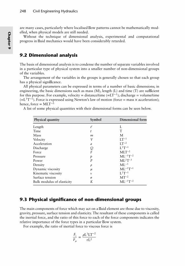
248 Civil Engineering Hydraulics
are many cases, particularly where localised flow patterns cannot be mathematically mod-elled, when physical models are still needed.
Without the technique of dimensional analysis, experimental and computationalprogress in fluid mechanics would have been considerably retarded.
9.2 Dimensional analysis
The basis of dimensional analysis is to condense the number of separate variables involvedin a particular type of physical system into a smaller number of non-dimensional groupsof the variables.
The arrangement of the variables in the groups is generally chosen so that each grouphas a physical significance.
All physical parameters can be expressed in terms of a number of basic dimensions; inengineering, the basic dimensions such as mass (M), length (L) and time (T) are sufficientfor this purpose. For example, velocity = distance/time (=LT−1); discharge = volume/time(=L3T−1). Force is expressed using Newton’s law of motion (force = mass × acceleration);hence, force = MLT−2.
A list of some physical quantities with their dimensional forms can be seen below.
Physical quantity Symbol Dimensional form
Length 𝓁 LTime t TMass m MVelocity V LT−1
Acceleration a LT−2
Discharge Q L3T−1
Force F MLT−2
Pressure p ML−1T−2
Power P ML2T−3
Density 𝜌 ML−3
Dynamic viscosity 𝜇 ML−1T−1
Kinematic viscosity 𝜈 L2T−1
Surface tension 𝜎 MT−2
Bulk modulus of elasticity K ML−1T−2
9.3 Physical significance of non-dimensional groups
The main components of force which may act on a fluid element are those due to viscosity,gravity, pressure, surface tension and elasticity. The resultant of these components is calledthe inertial force, and the ratio of this force to each of the force components indicates therelative importance of the force types in a particular flow system.
For example, the ratio of inertial force to viscous force is
Fi
F𝜇= 𝜌L3LT−2
𝜏L2
Ch
apter
9
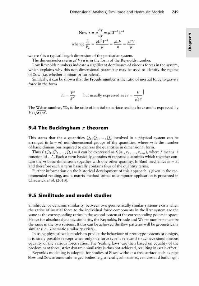
Dimensional Analysis, Similitude and Hydraulic Models 249
Now 𝜏 = 𝜇dy
dy= 𝜇LT−1L−1
whenceFi
F𝜇= 𝜌L2T−1
𝜇= 𝜌LV
𝜇= 𝜌𝓁V
𝜇
where 𝓁 is a typical length dimension of the particular system.The dimensionless term 𝜌𝓁V∕𝜇 is in the form of the Reynolds number.Low Reynolds numbers indicate a significant dominance of viscous forces in the system,
which explains why this non-dimensional parameter may be used to identify the regimeof flow (i.e. whether laminar or turbulent).
Similarly, it can be shown that the Froude number is the ratio of inertial force to gravityforce in the form
Fr = V2
g𝓁
(but usually expressed as Fr = V√
g𝓁
)
The Weber number, We, is the ratio of inertial to surface tension force and is expressed byV∕
√𝜎∕𝜌𝓁.
9.4 The Buckingham 𝝅 theorem
This states that the n quantities Q1, Q2,… , Qn involved in a physical system can bearranged in (n − m) non-dimensional groups of the quantities, where m is the numberof basic dimensions required to express the quantities in dimensional form.
Thus f1(Q1, Q2,… , Qn) = 0 can be expressed as f2(𝜋1,𝜋2,… ,𝜋n−m), where f means ‘afunction of …’ . Each 𝜋 term basically contains m repeated quantities which together con-tain the m basic dimensions together with one other quantity. In fluid mechanics m = 3,and therefore each 𝜋 term basically contains four of the quantity terms.
Further information on the historical development of this approach is given in the rec-ommended reading, and a matrix method suited to computer application is presented inChadwick et al. (2013).
9.5 Similitude and model studies
Similitude, or dynamic similarity, between two geometrically similar systems exists whenthe ratios of inertial force to the individual force components in the first system are thesame as the corresponding ratios in the second system at the corresponding points in space.Hence for absolute dynamic similarity, the Reynolds, Froude and Weber numbers must bethe same in the two systems. If this can be achieved the flow patterns will be geometricallysimilar (i.e., kinematic similarity exists).
In using physical scale models to predict the behaviour of prototype systems or designs,it is rarely possible (except when only one force type is relevant) to achieve simultaneousequality of the various force ratios. The ‘scaling laws’ are then based on equality of thepredominant force; strict dynamic similarity is thus not achieved, resulting in ‘scale effect’.
Reynolds modelling is adopted for studies of flows without a free surface such as pipeflow and flow around submerged bodies (e.g. aircraft, submarines, vehicles and buildings).
Ch
apte
r9
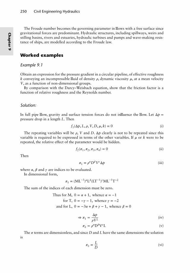
250 Civil Engineering Hydraulics
The Froude number becomes the governing parameter in flows with a free surface sincegravitational forces are predominant. Hydraulic structures, including spillways, weirs andstilling basins, rivers and estuaries, hydraulic turbines and pumps and wave-making resis-tance of ships, are modelled according to the Froude law.
Worked examples
Example 9.1
Obtain an expression for the pressure gradient in a circular pipeline, of effective roughnessk conveying an incompressible fluid of density 𝜌, dynamic viscosity 𝜇, at a mean velocityV, as a function of non-dimensional groups.
By comparison with the Darcy–Weisbach equation, show that the friction factor is afunction of relative roughness and the Reynolds number.
Solution:
In full pipe flow, gravity and surface tension forces do not influence the flow. Let Δp =pressure drop in a length L. Then
f1(Δp, L, 𝜌, V, D,𝜇, k) = 0 (i)
The repeating variables will be 𝜌, V and D. Δp clearly is not to be repeated since thisvariable is required to be expressed in terms of the other variables. If 𝜇 or k were to berepeated, the relative effect of the parameter would be hidden.
f2(𝜋1,𝜋2,𝜋3,𝜋4) = 0 (ii)
Then
𝜋1 = 𝜌𝛼D𝛽V𝛾Δp (iii)
where 𝛼, 𝛽 and 𝛾 are indices to be evaluated.In dimensional form,
𝜋1 = (ML−3)𝛼L𝛽(LT−1)𝛾ML−1T−2
The sum of the indices of each dimension must be zero.
Thus for M, 0 = 𝛼 + 1, whence 𝛼 = −1
for T, 0 = −𝛾 − 1, whence 𝛾 = −2
and for L, 0 = −3𝛼 + 𝛽 + 𝛾 − 1, whence 𝛽 = 0
⇒ 𝜋1 =Δp
𝜌V2(iv)
𝜋2 = 𝜌𝛼D𝛽V𝛾L (v)
The 𝜋 terms are dimensionless, and since D and L have the same dimensions the solutionis
𝜋2 = LD
(vi)
Ch
apter
9
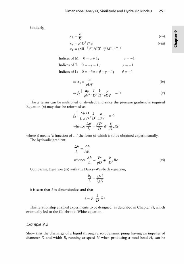
Dimensional Analysis, Similitude and Hydraulic Models 251
Similarly,
𝜋3 = kD
(vii)
𝜋4 = 𝜌𝛼D𝛽V𝛾𝜇 (viii)
𝜋4 = (ML−3)𝛼L𝛽(LT−1)𝛾ML−1T−1
Indices of M: 0 = 𝛼 + 1; 𝛼 = −1
Indices of T: 0 = −𝛾 − 1; 𝛾 = −1
Indices of L: 0 = −3𝛼 + 𝛽 + 𝛾 − 1; 𝛽 = −1
⇒ 𝜋4 = 𝜇
𝜌DV(ix)
⇒ f2
(Δp
𝜌V2, L
D, k
D,𝜇
𝜌DV
)= 0 (x)
The 𝜋 terms can be multiplied or divided, and since the pressure gradient is requiredEquation (x) may thus be reformed as
f2
(Δp D
L 𝜌V2, k
D,𝜇
𝜌DV
)= 0
whenceΔpL
= 𝜌V2
D𝜙
[kD
, Re]
where 𝜙 means ‘a function of …’ the form of which is to be obtained experimentally.The hydraulic gradient,
ΔhL
=Δp𝜌gL
whence ΔhL
= V2
gD𝜙
[kD
, Re]
(xi)
Comparing Equation (xi) with the Darcy–Weisbach equation,
hf
L= 𝜆V2
2gD
it is seen that 𝜆 is dimensionless and that
𝜆 = 𝜙
[kD
, Re]
This relationship enabled experiments to be designed (as described in Chapter 7), whicheventually led to the Colebrook–White equation.
Example 9.2
Show that the discharge of a liquid through a rotodynamic pump having an impeller ofdiameter D and width B, running at speed N when producing a total head H, can be
Ch
apte
r9
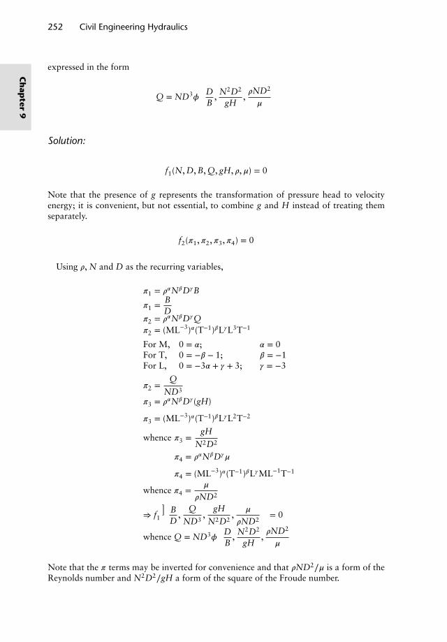
252 Civil Engineering Hydraulics
expressed in the form
Q = ND3𝜙
[DB
, N2D2
gH,𝜌ND2
𝜇
]
Solution:
f1(N, D, B, Q, gH, 𝜌,𝜇) = 0
Note that the presence of g represents the transformation of pressure head to velocityenergy; it is convenient, but not essential, to combine g and H instead of treating themseparately.
f2(𝜋1,𝜋2,𝜋3,𝜋4) = 0
Using 𝜌, N and D as the recurring variables,
𝜋1 = 𝜌𝛼N𝛽D𝛾B
𝜋1 = BD
𝜋2 = 𝜌𝛼N𝛽D𝛾Q𝜋2 = (ML−3)𝛼(T−1)𝛽L𝛾L3T−1
For M, 0 = 𝛼; 𝛼 = 0For T, 0 = −𝛽 − 1; 𝛽 = −1For L, 0 = −3𝛼 + 𝛾 + 3; 𝛾 = −3
𝜋2 =Q
ND3
𝜋3 = 𝜌𝛼N𝛽D𝛾 (gH)
𝜋3 = (ML−3)𝛼(T−1)𝛽L𝛾L2T−2
whence 𝜋3 =gH
N2D2
𝜋4 = 𝜌𝛼N𝛽D𝛾𝜇
𝜋4 = (ML−3)𝛼(T−1)𝛽L𝛾ML−1T−1
whence 𝜋4 = 𝜇
𝜌ND2
⇒ f1
(BD
,Q
ND3,
gH
N2D2,
𝜇
𝜌ND2
)= 0
whence Q = ND3𝜙
[DB
, N2D2
gH,𝜌ND2
𝜇
]
Note that the 𝜋 terms may be inverted for convenience and that 𝜌ND2∕𝜇 is a form of theReynolds number and N2D2∕gH a form of the square of the Froude number.
Ch
apter
9
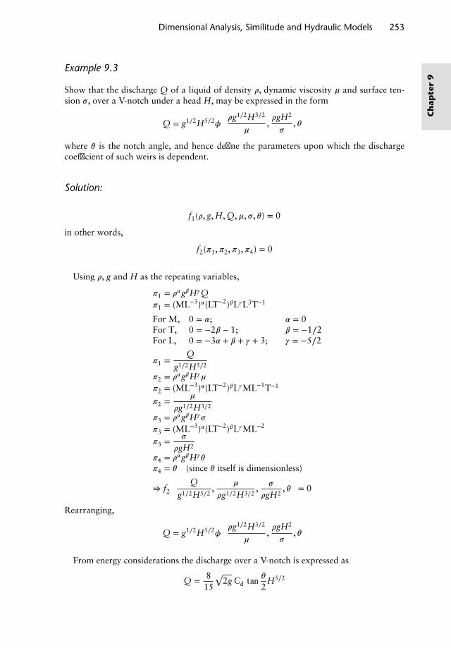
Dimensional Analysis, Similitude and Hydraulic Models 253
Example 9.3
Show that the discharge Q of a liquid of density 𝜌, dynamic viscosity 𝜇 and surface ten-sion 𝜎, over a V-notch under a head H, may be expressed in the form
Q = g1∕2H5∕2𝜙
[𝜌g1∕2H3∕2
𝜇,𝜌gH2
𝜎, 𝜃]
where 𝜃 is the notch angle, and hence define the parameters upon which the dischargecoefficient of such weirs is dependent.
Solution:
f1(𝜌, g, H, Q,𝜇, 𝜎, 𝜃) = 0
in other words,
f2(𝜋1,𝜋2,𝜋3,𝜋4) = 0
Using 𝜌, g and H as the repeating variables,
𝜋1 = 𝜌𝛼g𝛽H𝛾Q𝜋1 = (ML−3)𝛼(LT−2)𝛽L𝛾L3T−1
For M, 0 = 𝛼; 𝛼 = 0For T, 0 = −2𝛽 − 1; 𝛽 = −1∕2For L, 0 = −3𝛼 + 𝛽 + 𝛾 + 3; 𝛾 = −5∕2
𝜋1 =Q
g1∕2H5∕2
𝜋2 = 𝜌𝛼g𝛽H𝛾𝜇
𝜋2 = (ML−3)𝛼(LT−2)𝛽L𝛾ML−1T−1
𝜋2 = 𝜇
𝜌g1∕2H3∕2
𝜋3 = 𝜌𝛼g𝛽H𝛾𝜎
𝜋3 = (ML−3)𝛼(LT−2)𝛽L𝛾ML−2
𝜋3 = 𝜎
𝜌gH2
𝜋4 = 𝜌𝛼g𝛽H𝛾𝜃
𝜋4 = 𝜃 (since 𝜃 itself is dimensionless)
⇒ f2
[Q
g1∕2H5∕2,
𝜇
𝜌g1∕2H3∕2, 𝜎
𝜌gH2, 𝜃]= 0
Rearranging,
Q = g1∕2H5∕2𝜙
[𝜌g1∕2H3∕2
𝜇,𝜌gH2
𝜎, 𝜃]
From energy considerations the discharge over a V-notch is expressed as
Q = 815
√2g Cd tan 𝜃
2H5∕2
Ch
apte
r9
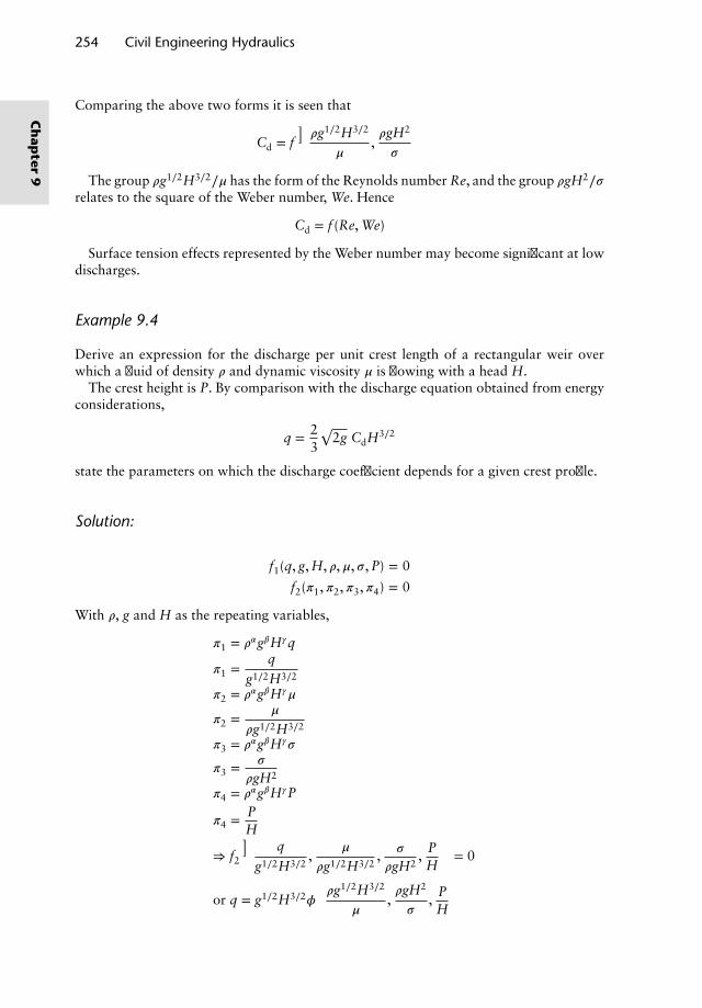
254 Civil Engineering Hydraulics
Comparing the above two forms it is seen that
Cd = f(𝜌g1∕2H3∕2
𝜇,𝜌gH2
𝜎
)
The group 𝜌g1∕2H3∕2∕𝜇 has the form of the Reynolds number Re, and the group 𝜌gH2∕𝜎relates to the square of the Weber number, We. Hence
Cd = f (Re, We)
Surface tension effects represented by the Weber number may become significant at lowdischarges.
Example 9.4
Derive an expression for the discharge per unit crest length of a rectangular weir overwhich a fluid of density 𝜌 and dynamic viscosity 𝜇 is flowing with a head H.
The crest height is P. By comparison with the discharge equation obtained from energyconsiderations,
q = 23
√2g CdH3∕2
state the parameters on which the discharge coefficient depends for a given crest profile.
Solution:
f1(q, g, H, 𝜌,𝜇, 𝜎, P) = 0
f2(𝜋1,𝜋2,𝜋3,𝜋4) = 0
With 𝜌, g and H as the repeating variables,
𝜋1 = 𝜌𝛼g𝛽H𝛾q
𝜋1 =q
g1∕2H3∕2
𝜋2 = 𝜌𝛼g𝛽H𝛾𝜇
𝜋2 = 𝜇
𝜌g1∕2H3∕2
𝜋3 = 𝜌𝛼g𝛽H𝛾𝜎
𝜋3 = 𝜎
𝜌gH2
𝜋4 = 𝜌𝛼g𝛽H𝛾P
𝜋4 = PH
⇒ f2
(q
g1∕2H3∕2,
𝜇
𝜌g1∕2H3∕2, 𝜎
𝜌gH2, P
H
)= 0
or q = g1∕2H3∕2𝜙
[𝜌g1∕2H3∕2
𝜇,𝜌gH2
𝜎, P
H
]
Ch
apter
9
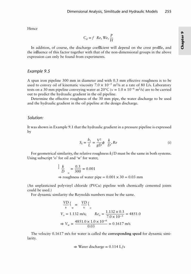
Dimensional Analysis, Similitude and Hydraulic Models 255
Hence
Cd = f[Re, We, P
H
]In addition, of course, the discharge coefficient will depend on the crest profile, and
the influence of this factor together with that of the non-dimensional groups in the aboveexpression can only be found from experiments.
Example 9.5
A spun iron pipeline 300 mm in diameter and with 0.3 mm effective roughness is to beused to convey oil of kinematic viscosity 7.0 × 10⁻⁵ m2/s at a rate of 80 L/s. Laboratorytests on a 30 mm pipeline conveying water at 20◦C (𝜈 = 1.0 × 10⁻⁶ m2/s) are to be carriedout to predict the hydraulic gradient in the oil pipeline.
Determine the effective roughness of the 30 mm pipe, the water discharge to be usedand the hydraulic gradient in the oil pipeline at the design discharge.
Solution:
It was shown in Example 9.1 that the hydraulic gradient in a pressure pipeline is expressedby
Sf =hf
L= V2
gD𝜙
[kD
, Re]
(i)
For geometrical similarity, the relative roughness k∕D must be the same in both systems.Using subscript ‘o’ for oil and ‘w’ for water,(
kD
)o= 0.3
300= 0.001
⇒ roughness of water pipe = 0.001 × 30 = 0.03 mm
(An unplasticised polyvinyl chloride (PVCu) pipeline with chemically cemented jointscould be used.)
For dynamic similarity the Reynolds numbers must be the same.
(VD𝜈
)w=(VD𝜈
)o
Vo = 1.132 m/s; Reo = 1.132 × 0.37.0 × 10−5
= 4851.0
⇒ Vw = 4851.0 × 1.0 × 10−6
0.03= 0.1617 m/s
The velocity 0.1617 m/s for water is called the corresponding speed for dynamic simi-larity.
⇒ Water discharge = 0.114 L∕s
Ch
apte
r9
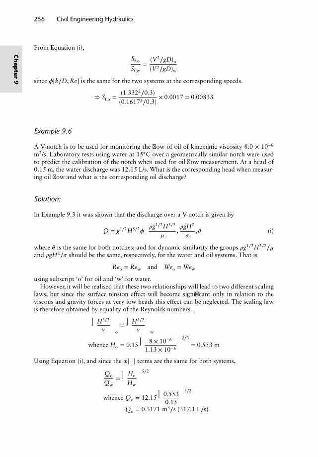
256 Civil Engineering Hydraulics
From Equation (i),
Sf,o
Sf,w=
(V2∕gD)o
(V2∕gD)w
since 𝜙[k∕D, Re] is the same for the two systems at the corresponding speeds.
⇒ Sf,o =(1.3322∕0.3)(0.16172∕0.3)
× 0.0017 = 0.00833
Example 9.6
A V-notch is to be used for monitoring the flow of oil of kinematic viscosity 8.0 × 10⁻⁶
m2/s. Laboratory tests using water at 15◦C over a geometrically similar notch were usedto predict the calibration of the notch when used for oil flow measurement. At a head of0.15 m, the water discharge was 12.15 L/s. What is the corresponding head when measur-ing oil flow and what is the corresponding oil discharge?
Solution:
In Example 9.3 it was shown that the discharge over a V-notch is given by
Q = g1∕2H5∕2𝜙
[𝜌g1∕2H3∕2
𝜇,𝜌gH2
𝜎, 𝜃]
(i)
where 𝜃 is the same for both notches; and for dynamic similarity the groups 𝜌g1∕2H3∕2∕𝜇and 𝜌gH2∕𝜎 should be the same, respectively, for the water and oil systems. That is
Reo = Rew and Weo = Wew
using subscript ‘o’ for oil and ‘w’ for water.However, it will be realised that these two relationships will lead to two different scaling
laws, but since the surface tension effect will become significant only in relation to theviscous and gravity forces at very low heads this effect can be neglected. The scaling lawis therefore obtained by equality of the Reynolds numbers.(
H3∕2
𝜈
)o=(
H3∕2
𝜈
)w
whence Ho = 0.15(
8 × 10⁻⁶
1.13 × 10⁻⁶
)2∕3
= 0.553 m
Using Equation (i), and since the 𝜙[ ] terms are the same for both systems,
Qo
Qw=(
Ho
Hw
)5∕2
whence Qo = 12.15(
0.5530.15
)5∕2
Qo = 0.3171 m3∕s (317.1 L∕s)
Ch
apter
9
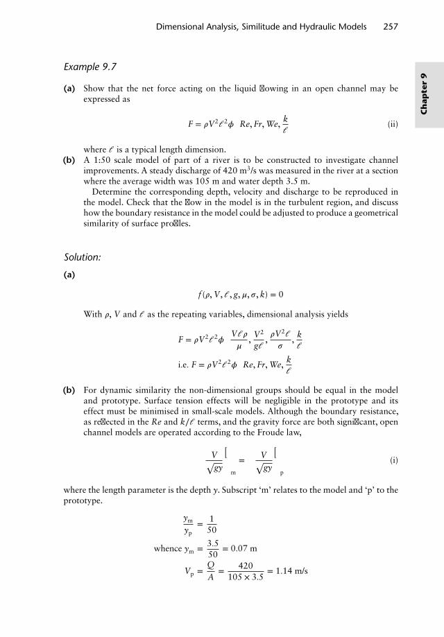
Dimensional Analysis, Similitude and Hydraulic Models 257
Example 9.7
(a) Show that the net force acting on the liquid flowing in an open channel may beexpressed as
F = 𝜌V2𝓁2𝜙
[Re, Fr, We, k
𝓁
](ii)
where 𝓁 is a typical length dimension.(b) A 1:50 scale model of part of a river is to be constructed to investigate channel
improvements. A steady discharge of 420 m3/s was measured in the river at a sectionwhere the average width was 105 m and water depth 3.5 m.
Determine the corresponding depth, velocity and discharge to be reproduced inthe model. Check that the flow in the model is in the turbulent region, and discusshow the boundary resistance in the model could be adjusted to produce a geometricalsimilarity of surface profiles.
Solution:
(a)
f (𝜌, V,𝓁, g,𝜇, 𝜎, k) = 0
With 𝜌, V and 𝓁 as the repeating variables, dimensional analysis yields
F = 𝜌V2𝓁2𝜙
[V𝓁𝜌𝜇
, V2
g𝓁,𝜌V2𝓁𝜎
, k𝓁
]
i.e. F = 𝜌V2𝓁2𝜙
[Re, Fr, We, k
𝓁
]
(b) For dynamic similarity the non-dimensional groups should be equal in the modeland prototype. Surface tension effects will be negligible in the prototype and itseffect must be minimised in small-scale models. Although the boundary resistance,as reflected in the Re and k∕𝓁 terms, and the gravity force are both significant, openchannel models are operated according to the Froude law,(
V√gy
)m
=
(V√gy
)p
(i)
where the length parameter is the depth y. Subscript ‘m’ relates to the model and ‘p’ to theprototype.
ym
yp= 1
50
whence ym = 3.550
= 0.07 m
Vp =QA
= 420105 × 3.5
= 1.14 m/s
Ch
apte
r9
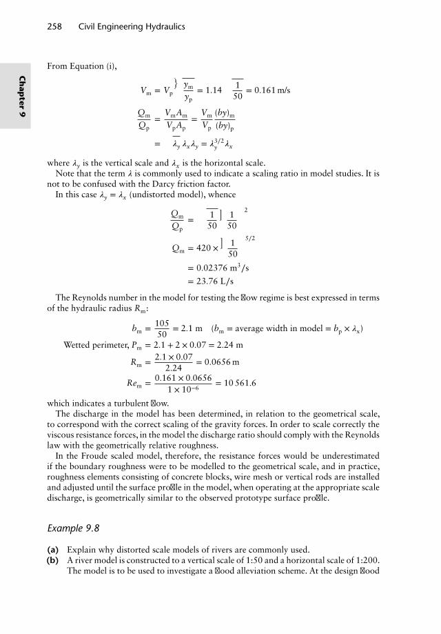
258 Civil Engineering Hydraulics
From Equation (i),
Vm = Vp
√ym
yp= 1.14
√1
50= 0.161 m/s
Qm
Qp=
VmAm
VpAp=
Vm
Vp
(by)m
(by)p
=√𝜆y 𝜆x𝜆y = 𝜆3∕2
y 𝜆x
where 𝜆y is the vertical scale and 𝜆x is the horizontal scale.Note that the term 𝜆 is commonly used to indicate a scaling ratio in model studies. It is
not to be confused with the Darcy friction factor.In this case 𝜆y = 𝜆x (undistorted model), whence
Qm
Qp=√
150
(150
)2
Qm = 420 ×(
150
)5∕2
= 0.02376 m3∕s
= 23.76 L∕s
The Reynolds number in the model for testing the flow regime is best expressed in termsof the hydraulic radius Rm:
bm = 10550
= 2.1 m (bm = average width in model = bp × 𝜆x)
Wetted perimeter, Pm = 2.1 + 2 × 0.07 = 2.24 m
Rm = 2.1 × 0.072.24
= 0.0656 m
Rem = 0.161 × 0.06561 × 10−6
= 10 561.6
which indicates a turbulent flow.The discharge in the model has been determined, in relation to the geometrical scale,
to correspond with the correct scaling of the gravity forces. In order to scale correctly theviscous resistance forces, in the model the discharge ratio should comply with the Reynoldslaw with the geometrically relative roughness.
In the Froude scaled model, therefore, the resistance forces would be underestimatedif the boundary roughness were to be modelled to the geometrical scale, and in practice,roughness elements consisting of concrete blocks, wire mesh or vertical rods are installedand adjusted until the surface profile in the model, when operating at the appropriate scaledischarge, is geometrically similar to the observed prototype surface profile.
Example 9.8
(a) Explain why distorted scale models of rivers are commonly used.(b) A river model is constructed to a vertical scale of 1:50 and a horizontal scale of 1:200.
The model is to be used to investigate a flood alleviation scheme. At the design flood
Ch
apter
9
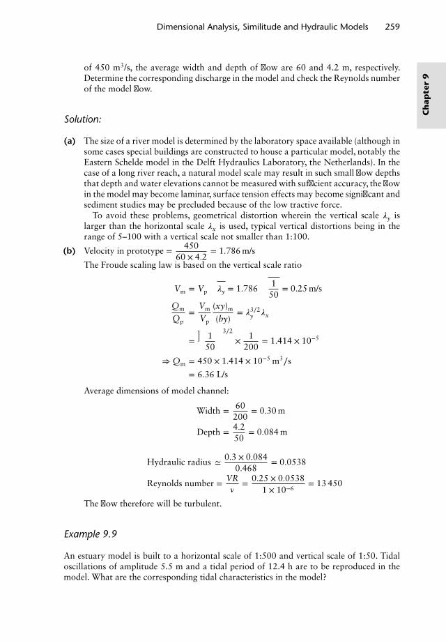
Dimensional Analysis, Similitude and Hydraulic Models 259
of 450 m3/s, the average width and depth of flow are 60 and 4.2 m, respectively.Determine the corresponding discharge in the model and check the Reynolds numberof the model flow.
Solution:
(a) The size of a river model is determined by the laboratory space available (although insome cases special buildings are constructed to house a particular model, notably theEastern Schelde model in the Delft Hydraulics Laboratory, the Netherlands). In thecase of a long river reach, a natural model scale may result in such small flow depthsthat depth and water elevations cannot be measured with sufficient accuracy, the flowin the model may become laminar, surface tension effects may become significant andsediment studies may be precluded because of the low tractive force.
To avoid these problems, geometrical distortion wherein the vertical scale 𝜆y islarger than the horizontal scale 𝜆x is used, typical vertical distortions being in therange of 5–100 with a vertical scale not smaller than 1:100.
(b) Velocity in prototype = 45060 × 4.2
= 1.786 m/s
The Froude scaling law is based on the vertical scale ratio
Vm = Vp
√𝜆y = 1.786
√150
= 0.25 m/s
Qm
Qp=
Vm
Vp
(xy)m
(by)= 𝜆3∕2
y 𝜆x
=(
150
)3∕2
× 1200
= 1.414 × 10⁻⁵
⇒ Qm = 450 × 1.414 × 10−5 m3∕s
= 6.36 L/s
Average dimensions of model channel:
Width = 60200
= 0.30 m
Depth = 4.250
= 0.084 m
Hydraulic radius ≃ 0.3 × 0.0840.468
= 0.0538
Reynolds number = VR𝜈
= 0.25 × 0.05381 × 10−6
= 13 450
The flow therefore will be turbulent.
Example 9.9
An estuary model is built to a horizontal scale of 1:500 and vertical scale of 1:50. Tidaloscillations of amplitude 5.5 m and a tidal period of 12.4 h are to be reproduced in themodel. What are the corresponding tidal characteristics in the model?
Ch
apte
r9
260 Civil Engineering Hydraulics
Solution:
The speed of propagation, or celerity, of a gravity wave in which the wavelength is verylarge in relation to the water depth y, as in the case of tidal oscillations, is given by c =
√gy.
Thus, estuary models must be operated according to the Froude law.The tidal range is modelled according to the vertical scale.
Hm = Hp ×1
50= 5.5
50= 0.11 m
Tidal period, T = Lc
where L is the wavelength. Hence
Tm
Tp=
Lm
Lp
cp
cm= 𝜆x
√yp
ym=
𝜆x√𝜆y
⇒ Tm =12.4 × 1∕500√
1∕50= 0.1754 h
= 10.52 min
Example 9.10
The discharge Q from a rotodynamic pump developing a total head H when running atN revolutions per minute is given by
Q = ND3𝜙
[DB
, N2D2
gH,𝜌ND2
𝜇
](see Example 9.2) (i)
(a) Obtain an expression for the specific speed of a rotodynamic pump and show howto predict the pump characteristics when running at different speeds.
(b) The performance of a new design of rotodynamic pump is to be tested in a 1:5 scalemodel. The pump is to run at 1450 rev/min.
The model delivers a discharge of 2.5 L/s of water and a total head of 3 m, with anefficiency of 65% when operating at 2000 rev/min. What are the corresponding dischargehead and power consumption in the prototype? Determine the specific speed of the pumpand hence state the type of impeller.
Solution:
(a) For geometrically similar machines operating at high Reynolds numbers, the term𝜌ND2∕𝜇 becomes unimportant and Equation (i) may be rewritten as
f(
Q
ND3, D
B, N2D2
gH
)= 0
Ch
apter
9
Dimensional Analysis, Similitude and Hydraulic Models 261
The term D∕B is automatically satisfied by the geometrical similarity, and the termsQ∕ND3 and N2D2∕gH should have identical values in the model and prototype.
⇒
(Q
ND3
)m=(
Q
ND3
)p
(ii)
and(
N2D2
gH
)m=(
N2D2
gH
)p
(iii)
The scale
Dm
Dp=
Np
Nm
(Hm
Hp
)1∕2
(from Equation (iii))
whence from Equation (ii)
Nm
Np=
√QP
Qm
(Hm
Hp
)3∕4
(iv)
If Hm and Qm are made equal to unity, then Equation (iv) becomes
Nm =Np
√Qp
H3∕4p
(v)
The term N√
Q∕H3∕4 is called the specific speed and is interpreted as the speedat which a geometrically scaled model would run in order to deliver unit dischargewhen generating unit head. All geometrically similar machines have the same specificspeed.
In the case of the same pump running at different speeds, Dm = Dp and Equa-tion (ii) becomes
Q1
N1=
Q2
N2or Q2 = Q1
(N2
N1
)
and Equation (iii) becomes
N1
H21
=N2
H22
or H2 = H1
√N2
N1
(b) From Equation (ii)
Qp = Qm
(ND3)p
(ND3)m
⇒ Qp = 2.5 × 53 × 14502000
= 226 L∕s
From Equation (iii)
Hp = Hm
( Np
Nm
Dp
Dm
)2
= 3.0(
14502000
× 5)2
= 39.42 m
Ch
apte
r9
262 Civil Engineering Hydraulics
Power input required = 9.81 × 0.226 × 39.420.65
= 134.5 kW
Specific speed, Ns =N√
Q
H3∕4=
1450√
226(39.42)3∕4
= 1385
The impeller is of the centrifugal type (see Chapter 6).
Example 9.11
A model of a proposed dam spillway was constructed to a scale of 1:25. The design flooddischarge over the spillway is 1000 m3/s. What discharge should be provided in the model?What is the velocity in the prototype corresponding with a velocity of 1.5 m/s in the modelat the corresponding point?
Solution:
Example 9.4 showed that the discharge per unit crest length of a rectangular weir couldbe expressed as
q = g1∕2H3∕2𝜙
[𝜌g1∕2H3∕2
𝜇,𝜌gH2
𝜎, P
H
](i)
The governing equation for spillways and weirs is identical. Flood discharges over spill-ways will result in very high Reynolds numbers, and since surface tension effects are alsonegligible the only factor affecting the discharge coefficient is P∕H. In modelling dam spill-ways, therefore, if the ratios of P∕H in the model and prototype are identical and the crestgeometry is correctly scaled,
q
g1∕2H3∕2= Constant
Therefore, spillway models are operated according to the Froude law and are madesufficiently large that viscous and surface tension effects are negligible.(
V√g𝓁
)m
=
(V√g𝓁
)p
(ii)
Q = V𝓁2 (iii)
⇒
(Q
𝓁5∕2
)m=(
Q
𝓁5∕2
)p
(iv)
whence
Qm = 1000(
125
)5∕2
= 0.32 m3∕s
From Equation (ii)
Vp = Vm
√𝓁p
𝓁m= Vm
√25
⇒ Vp = 1.5 × 5 = 7.5 m/s
Ch
apter
9
Dimensional Analysis, Similitude and Hydraulic Models 263
References and recommended reading
Allen, J. (1952) Scale Models in Hydraulic Engineering, Longman, London.Chadwick, A., Morfett, J. and Borthwick, M. (2013) Hydraulics in Civil and Environmental
Engineering, 5th edn, Taylor & Francis, Abingdon, UK.Novak, P. and Cabelka, J. (1981) Models in Hydraulic Engineering, Pitman, London.Webber, N. B. (1971) Fluid Mechanics for Civil Engineers, Spon, London.Yalin, M. S. (1971) Theory of Hydraulic Models, Macmillan, London.
Problems
1. The head loss of water of kinematic viscosity 1 × 10⁻⁶ m2∕s in a 50 mm diameter pipelinewas 0.25 m over a length of 10.0 m at a discharge of 2.0 L/s. What is the correspondingdischarge and hydraulic gradient when oil of kinematic viscosity 8.5 × 10⁻⁶ m2∕s flowsthrough a 250 mm diameter pipeline of the same relative roughness?
2. Find the pressure drop at the corresponding speed in a pipe 25 mm in diameter and30 m long conveying water at 10◦C if the pressure head loss in a 200 mm diameter smoothpipe 300 m long in which air is flowing at a velocity of 3 m/s is 10 mm of water. Densityof air = 1.3 kg∕m3; dynamic viscosity of air = 1.77 × 10⁻⁵ N s∕m2; dynamic viscosity ofwater = 1.3 × 10⁻³ N s∕m2.
3. A 50 mm diameter pipe is used to convey air at 4◦C (density = 1.12 kg∕m3 and dynamicviscosity = 1.815 × 10⁻⁵ N s/m2) at a mean velocity of 20 m/s. Calculate the discharge ofwater at 20◦C for dynamic similarity, and obtain the ratio of the pressure drop per unitlength in the two cases.
4. If, in modelling a physical system, the Reynolds and Froude numbers are to be the samein the model and prototype, determine the ratio of kinematic viscosity of the fluid in themodel to that in the prototype.
5. The sequent depth ys of a hydraulic jump in a rectangular channel is related to the initialdepth yi, the discharge per unit width, q, g and p. Express the ratio ys∕yi in terms ofa non-dimensional group and compare with the equation developed from momentumprinciples:
ys =yi
2
(√1 + Fr2
i − 1)
6. A 60◦ V-notch is to be used for measuring the discharge of oil having a kinematic viscosity10 times that of water. The notch was calibrated using water. When the head over thenotch was 0.1 m the discharge was 2.54 L/s. Determine the corresponding head anddischarge when the notch is used for oil flow measurement.
7. The airflow and wind effects on a bridge structure are to be studied on a 1:25 scalemodel in a pressurised wind tunnel in which the air density is eight times that of air atatmospheric pressure and at the same temperature. If the bridge structure is subjectedto wind speeds of 30 m/s, what is the corresponding wind speed in the wind tunnel?What force on the prototype corresponds with a 1400 N force on the model? (Note:The dynamic viscosity of air is unaffected by pressure changes provided the temperatureremains constant.)
Ch
apte
r9
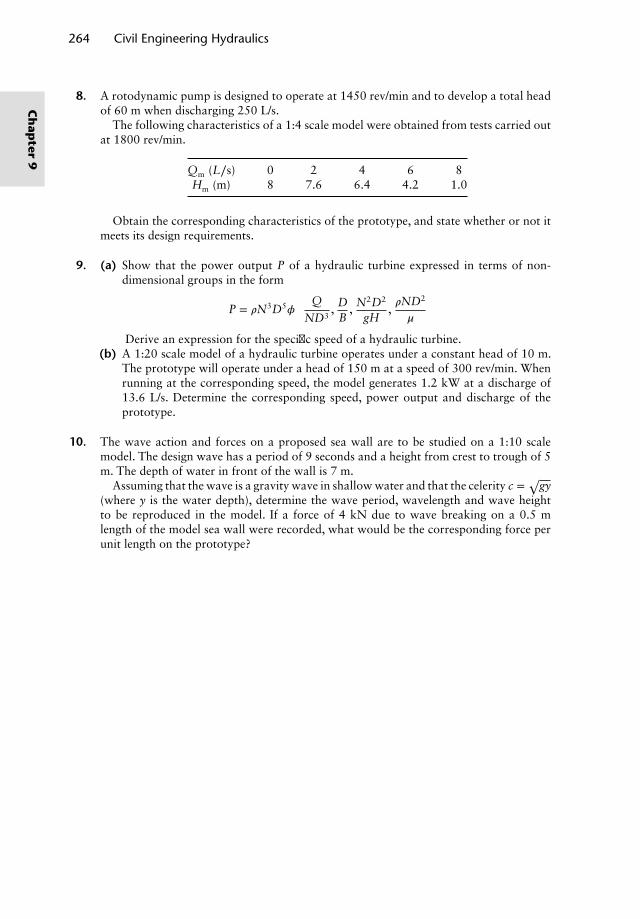
264 Civil Engineering Hydraulics
8. A rotodynamic pump is designed to operate at 1450 rev/min and to develop a total headof 60 m when discharging 250 L/s.
The following characteristics of a 1:4 scale model were obtained from tests carried outat 1800 rev/min.
Qm (L∕s) 0 2 4 6 8Hm (m) 8 7.6 6.4 4.2 1.0
Obtain the corresponding characteristics of the prototype, and state whether or not itmeets its design requirements.
9. (a) Show that the power output P of a hydraulic turbine expressed in terms of non-dimensional groups in the form
P = 𝜌N3D5𝜙
[Q
ND3, D
B, N2D2
gH,𝜌ND2
𝜇
]
Derive an expression for the specific speed of a hydraulic turbine.(b) A 1:20 scale model of a hydraulic turbine operates under a constant head of 10 m.
The prototype will operate under a head of 150 m at a speed of 300 rev/min. Whenrunning at the corresponding speed, the model generates 1.2 kW at a discharge of13.6 L/s. Determine the corresponding speed, power output and discharge of theprototype.
10. The wave action and forces on a proposed sea wall are to be studied on a 1:10 scalemodel. The design wave has a period of 9 seconds and a height from crest to trough of 5m. The depth of water in front of the wall is 7 m.
Assuming that the wave is a gravity wave in shallow water and that the celerity c =√
gy(where y is the water depth), determine the wave period, wavelength and wave heightto be reproduced in the model. If a force of 4 kN due to wave breaking on a 0.5 mlength of the model sea wall were recorded, what would be the corresponding force perunit length on the prototype?
Ch
apter
9
Chapter 10Ideal Fluid Flow andCurvilinear Flow
10.1 Ideal fluid flow
The analysis of ideal fluid flow is also referred to as potential flow. The concept of anideal fluid is that of one which is inviscid and incompressible; the flow is also assumedto be irrotational. Since flow in boundary layers is rotational and strongly influenced byviscosity, the analytical techniques of ideal fluid flow cannot be applied in such circum-stances. However, in many situations the flow of real fluids outside the boundary layer,where viscous effects are small, approximates closely to that of an ideal fluid.
The object of the study of ideal fluid flow is to obtain the flow pattern and pressure distri-bution in the fluid flow around prescribed boundaries. Examples are the flow over airfoils,through the passages of pump and turbine blades, over dam spillways and under controlgates. The governing differential equations of ideal fluid flow have also been successfullyapplied to oscillatory wave motions, groundwater and seepage flows.
10.2 Streamlines, the stream function
A streamline is a continuous line drawn through the fluid such that it is tangential tothe velocity vector at every point. In steady flow the streamlines are identical with thepathlines or tracks of discrete liquid elements. No flow can occur across a streamline, andthe concept of a stream tube in two-dimensional flow emerges as the flow per unit depthbetween adjacent streamlines.
From Figure 10.1a,
dy
dx= v
u; u dy − v dx = 0 [10.1]
The continuity equation for two-dimensional steady ideal fluid flow is
𝜕u𝜕x
+ 𝜕v𝜕y
= 0 [10.2]
Nalluri & Featherstone’s Civil Engineering Hydraulics: Essential Theory with Worked Examples,Sixth Edition. Martin Marriott.© 2016 John Wiley & Sons, Ltd. Published 2016 by John Wiley & Sons, Ltd.Companion Website: www.wiley.com/go/Marriott
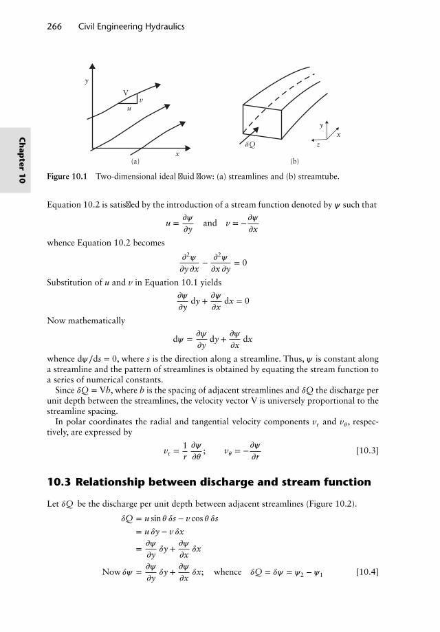
266 Civil Engineering Hydraulics
y
V
uv
x
xy
zδQ
(b)(a)
Figure 10.1 Two-dimensional ideal fluid flow: (a) streamlines and (b) streamtube.
Equation 10.2 is satisfied by the introduction of a stream function denoted by 𝜓 such that
u = 𝜕𝜓
𝜕yand v = −𝜕𝜓
𝜕x
whence Equation 10.2 becomes
𝜕2𝜓
𝜕y 𝜕x− 𝜕2𝜓
𝜕x 𝜕y= 0
Substitution of u and v in Equation 10.1 yields
𝜕𝜓
𝜕ydy + 𝜕𝜓
𝜕xdx = 0
Now mathematically
d𝜓 = 𝜕𝜓
𝜕ydy + 𝜕𝜓
𝜕xdx
whence d𝜓∕ds = 0, where s is the direction along a streamline. Thus, 𝜓 is constant alonga streamline and the pattern of streamlines is obtained by equating the stream function toa series of numerical constants.
Since 𝛿Q = Vb, where b is the spacing of adjacent streamlines and 𝛿Q the discharge perunit depth between the streamlines, the velocity vector V is universely proportional to thestreamline spacing.
In polar coordinates the radial and tangential velocity components vr and v𝜃, respec-tively, are expressed by
vr =1r𝜕𝜓
𝜕𝜃; v𝜃 = −𝜕𝜓
𝜕r[10.3]
10.3 Relationship between discharge and stream function
Let 𝛿Q be the discharge per unit depth between adjacent streamlines (Figure 10.2).
𝛿Q = u sin 𝜃 𝛿s − v cos 𝜃 𝛿s= u 𝛿y − v 𝛿x
= 𝜕𝜓
𝜕y𝛿y + 𝜕𝜓
𝜕x𝛿x
Now 𝛿𝜓 = 𝜕𝜓
𝜕y𝛿y + 𝜕𝜓
𝜕x𝛿x; whence 𝛿Q = 𝛿𝜓 = 𝜓2 − 𝜓1 [10.4]
Ch
apter
10
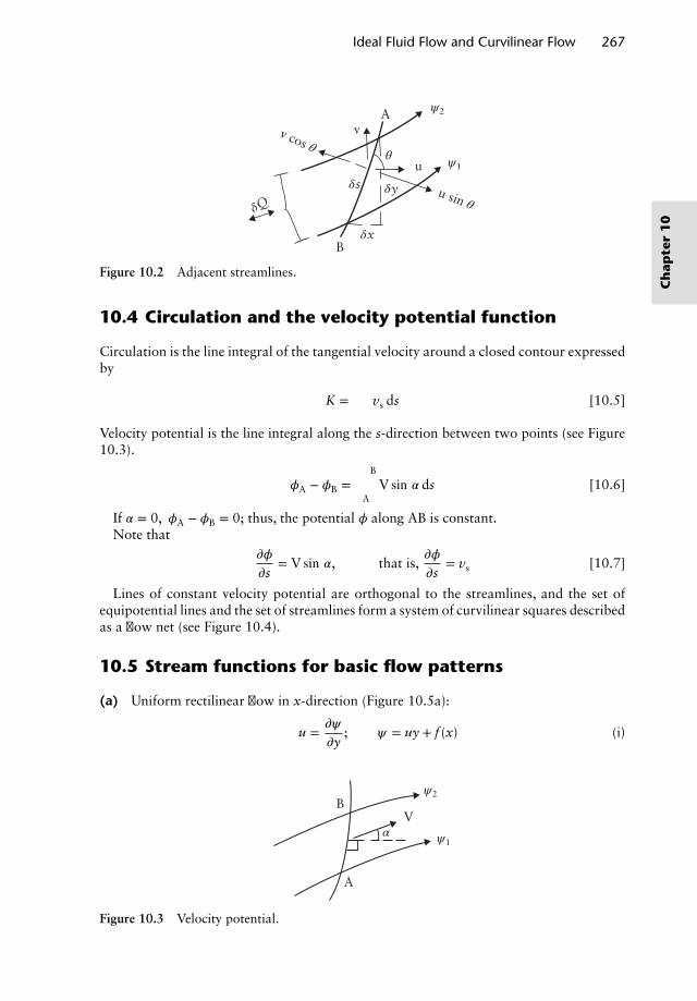
Ideal Fluid Flow and Curvilinear Flow 267
δQδs δy
θ
δx
ψ2
ψ1
v cos θ
u sin θ
B
Av
u
Figure 10.2 Adjacent streamlines.
10.4 Circulation and the velocity potential function
Circulation is the line integral of the tangential velocity around a closed contour expressedby
K = ∫ vs ds [10.5]
Velocity potential is the line integral along the s-direction between two points (see Figure10.3).
𝜙A − 𝜙B = ∫B
AV sin 𝛼 ds [10.6]
If 𝛼 = 0, 𝜙A − 𝜙B = 0; thus, the potential 𝜙 along AB is constant.Note that
𝜕𝜙
𝜕s= V sin 𝛼, that is,
𝜕𝜙
𝜕s= vs [10.7]
Lines of constant velocity potential are orthogonal to the streamlines, and the set ofequipotential lines and the set of streamlines form a system of curvilinear squares describedas a flow net (see Figure 10.4).
10.5 Stream functions for basic flow patterns
(a) Uniform rectilinear flow in x-direction (Figure 10.5a):
u = 𝜕𝜓
𝜕y; 𝜓 = uy + f (x) (i)
ψ2
ψ1α
A
BV
Figure 10.3 Velocity potential.
Ch
apte
r1
0
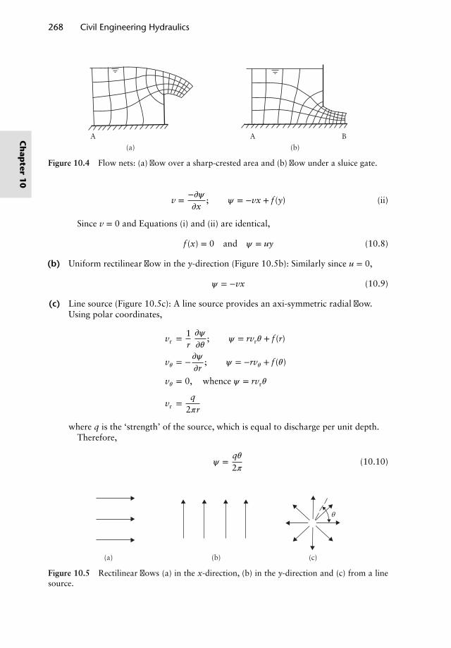
268 Civil Engineering Hydraulics
BAA
(b)(a)
Figure 10.4 Flow nets: (a) flow over a sharp-crested area and (b) flow under a sluice gate.
v = −𝜕𝜓𝜕x
; 𝜓 = −vx + f (y) (ii)
Since v = 0 and Equations (i) and (ii) are identical,
f (x) = 0 and 𝜓 = uy (10.8)
(b) Uniform rectilinear flow in the y-direction (Figure 10.5b): Similarly since u = 0,
𝜓 = −vx (10.9)
(c) Line source (Figure 10.5c): A line source provides an axi-symmetric radial flow.Using polar coordinates,
vr = 1r𝜕𝜓
𝜕𝜃; 𝜓 = rvr𝜃 + f (r)
v𝜃 = −𝜕𝜓𝜕r
; 𝜓 = −rv𝜃 + f (𝜃)
v𝜃 = 0, whence 𝜓 = rvr𝜃
vr =q
2𝜋r
where q is the ‘strength’ of the source, which is equal to discharge per unit depth.Therefore,
𝜓 =q𝜃2𝜋
(10.10)
(c)(b)(a)
θ
Figure 10.5 Rectilinear flows (a) in the x-direction, (b) in the y-direction and (c) from a linesource.
Ch
apter
10
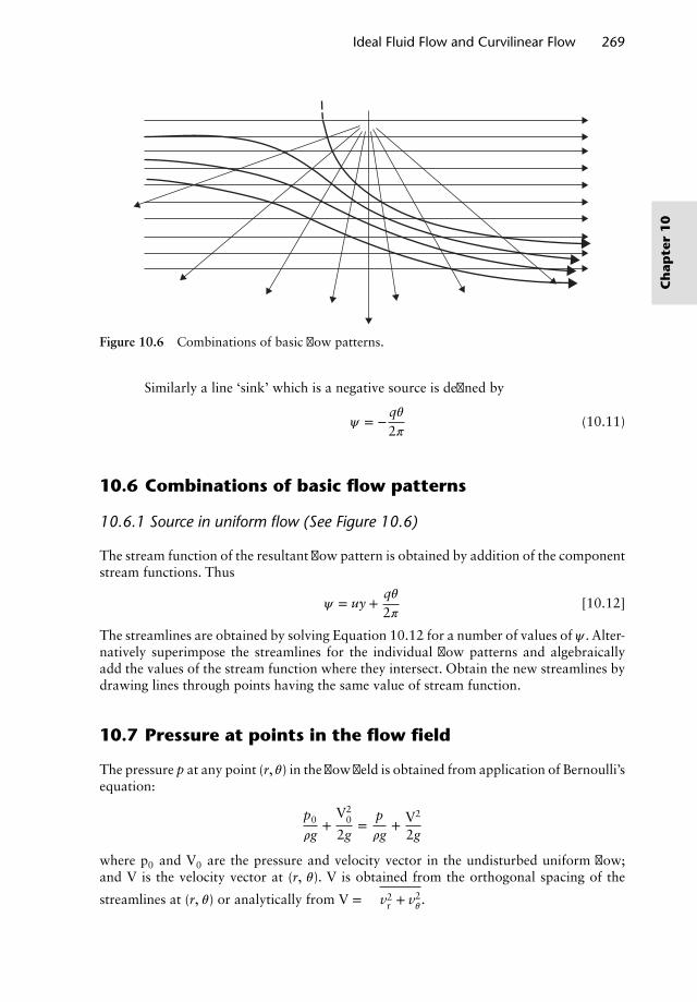
Ideal Fluid Flow and Curvilinear Flow 269
Figure 10.6 Combinations of basic flow patterns.
Similarly a line ‘sink’ which is a negative source is defined by
𝜓 = −q𝜃2𝜋
(10.11)
10.6 Combinations of basic flow patterns
10.6.1 Source in uniform flow (See Figure 10.6)
The stream function of the resultant flow pattern is obtained by addition of the componentstream functions. Thus
𝜓 = uy +q𝜃2𝜋
[10.12]
The streamlines are obtained by solving Equation 10.12 for a number of values of 𝜓 . Alter-natively superimpose the streamlines for the individual flow patterns and algebraicallyadd the values of the stream function where they intersect. Obtain the new streamlines bydrawing lines through points having the same value of stream function.
10.7 Pressure at points in the flow field
The pressure p at any point (r, 𝜃) in the flow field is obtained from application of Bernoulli’sequation:
p0
𝜌g+
V20
2g=
p𝜌g
+ V2
2g
where p0 and V0 are the pressure and velocity vector in the undisturbed uniform flow;and V is the velocity vector at (r, 𝜃). V is obtained from the orthogonal spacing of the
streamlines at (r, 𝜃) or analytically from V =√
v2r + v2
𝜃.
Ch
apte
r1
0
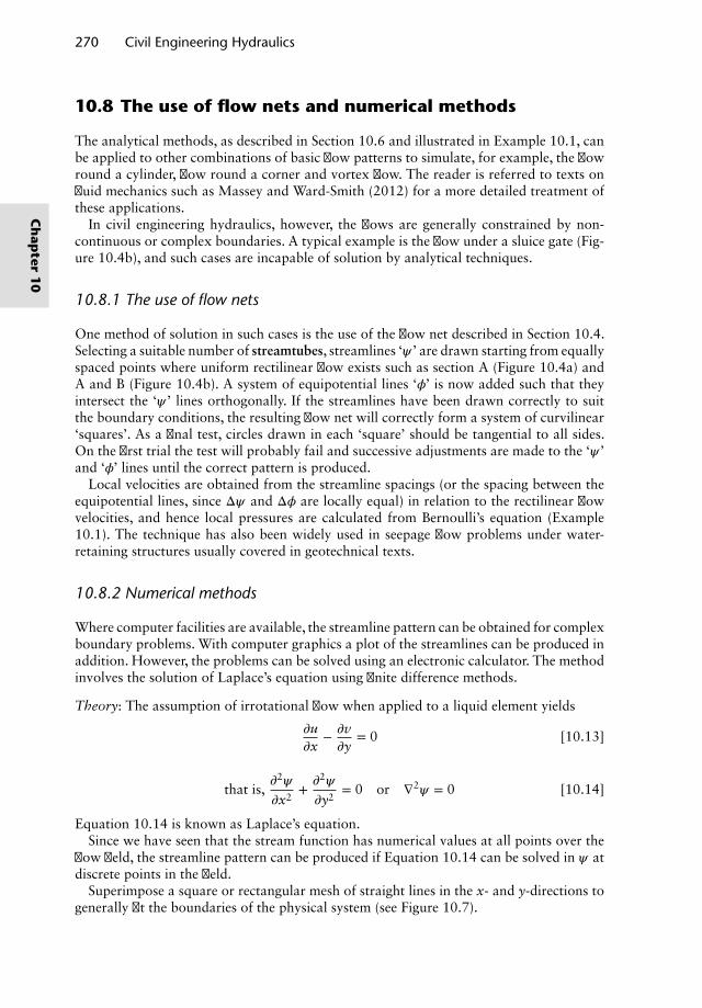
270 Civil Engineering Hydraulics
10.8 The use of flow nets and numerical methods
The analytical methods, as described in Section 10.6 and illustrated in Example 10.1, canbe applied to other combinations of basic flow patterns to simulate, for example, the flowround a cylinder, flow round a corner and vortex flow. The reader is referred to texts onfluid mechanics such as Massey and Ward-Smith (2012) for a more detailed treatment ofthese applications.
In civil engineering hydraulics, however, the flows are generally constrained by non-continuous or complex boundaries. A typical example is the flow under a sluice gate (Fig-ure 10.4b), and such cases are incapable of solution by analytical techniques.
10.8.1 The use of flow nets
One method of solution in such cases is the use of the flow net described in Section 10.4.Selecting a suitable number of streamtubes, streamlines ‘𝜓 ’ are drawn starting from equallyspaced points where uniform rectilinear flow exists such as section A (Figure 10.4a) andA and B (Figure 10.4b). A system of equipotential lines ‘𝜙’ is now added such that theyintersect the ‘𝜓 ’ lines orthogonally. If the streamlines have been drawn correctly to suitthe boundary conditions, the resulting flow net will correctly form a system of curvilinear‘squares’. As a final test, circles drawn in each ‘square’ should be tangential to all sides.On the first trial the test will probably fail and successive adjustments are made to the ‘𝜓 ’and ‘𝜙’ lines until the correct pattern is produced.
Local velocities are obtained from the streamline spacings (or the spacing between theequipotential lines, since Δ𝜓 and Δ𝜙 are locally equal) in relation to the rectilinear flowvelocities, and hence local pressures are calculated from Bernoulli’s equation (Example10.1). The technique has also been widely used in seepage flow problems under water-retaining structures usually covered in geotechnical texts.
10.8.2 Numerical methods
Where computer facilities are available, the streamline pattern can be obtained for complexboundary problems. With computer graphics a plot of the streamlines can be produced inaddition. However, the problems can be solved using an electronic calculator. The methodinvolves the solution of Laplace’s equation using finite difference methods.
Theory: The assumption of irrotational flow when applied to a liquid element yields
𝜕u𝜕x
− 𝜕v𝜕y
= 0 [10.13]
that is,𝜕2𝜓
𝜕x2+ 𝜕2𝜓
𝜕y2= 0 or ∇2𝜓 = 0 [10.14]
Equation 10.14 is known as Laplace’s equation.Since we have seen that the stream function has numerical values at all points over the
flow field, the streamline pattern can be produced if Equation 10.14 can be solved in 𝜓 atdiscrete points in the field.
Superimpose a square or rectangular mesh of straight lines in the x- and y-directions togenerally fit the boundaries of the physical system (see Figure 10.7).
Ch
apter
10
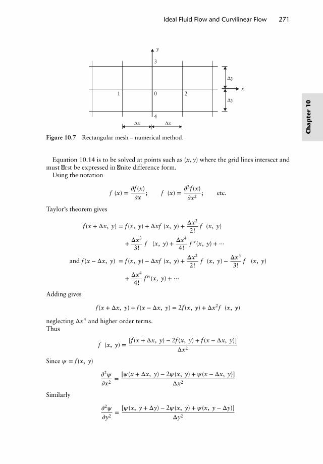
Ideal Fluid Flow and Curvilinear Flow 271
20
4Δx Δx
x
Δy
Δy
3
y
1
Figure 10.7 Rectangular mesh – numerical method.
Equation 10.14 is to be solved at points such as (x, y) where the grid lines intersect andmust first be expressed in finite difference form.
Using the notation
f ′(x) =𝜕f (x)𝜕x
; f ′′(x) =𝜕2f (x)𝜕x2
; etc.
Taylor’s theorem gives
f (x + Δx, y) = f (x, y) + Δxf ′(x, y) + Δx2
2!f ′′(x, y)
+ Δx3
3!f ′′′(x, y) + Δx4
4!f iv(x, y) +⋯
and f (x − Δx, y) = f (x, y) − Δxf ′(x, y) + Δx2
2!f ′′(x, y) − Δx3
3!f ′′′(x, y)
+ Δx4
4!f iv(x, y) +⋯
Adding gives
f (x + Δx, y) + f (x − Δx, y) = 2f (x, y) + Δx2f ′′(x, y)
neglecting Δx4 and higher order terms.Thus
f ′′(x, y) =[f (x + Δx, y) − 2f (x, y) + f (x − Δx, y)]
Δx2
Since 𝜓 = f (x, y)
𝜕2𝜓
𝜕x2=
[𝜓(x + Δx, y) − 2𝜓(x, y) + 𝜓(x − Δx, y)]Δx2
Similarly
𝜕2𝜓
𝜕y2=
[𝜓(x, y + Δy) − 2𝜓(x, y) + 𝜓(x, y − Δy)]Δy2
Ch
apte
r1
0
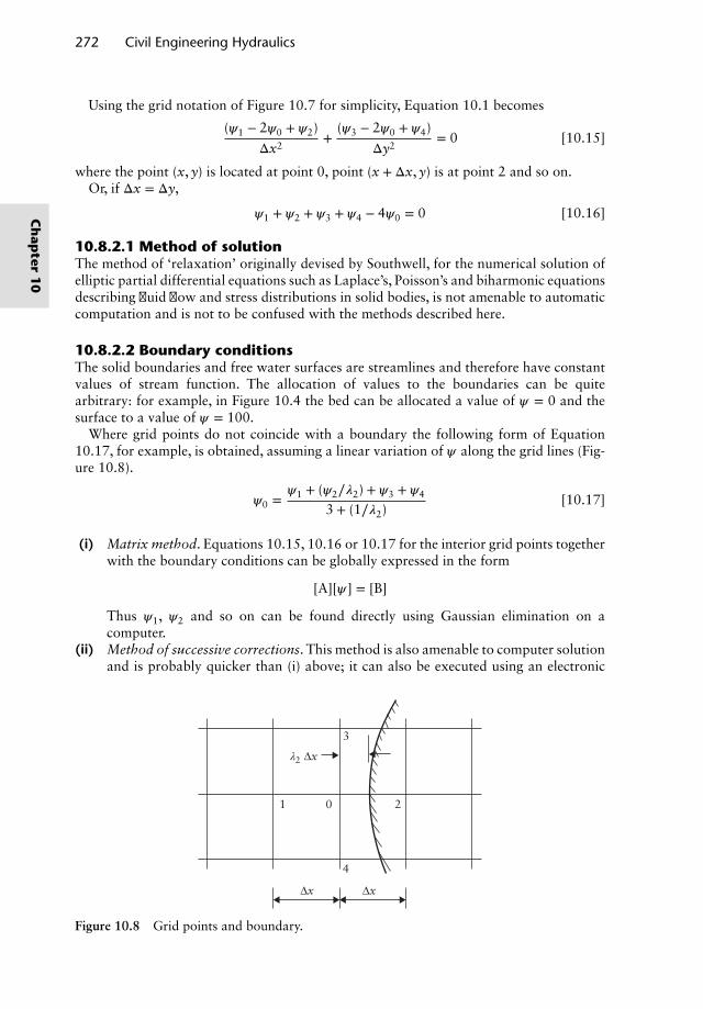
272 Civil Engineering Hydraulics
Using the grid notation of Figure 10.7 for simplicity, Equation 10.1 becomes
(𝜓1 − 2𝜓0 + 𝜓2)
Δx2+
(𝜓3 − 2𝜓0 + 𝜓4)
Δy2= 0 [10.15]
where the point (x, y) is located at point 0, point (x + Δx, y) is at point 2 and so on.Or, if Δx = Δy,
𝜓1 + 𝜓2 + 𝜓3 + 𝜓4 − 4𝜓0 = 0 [10.16]
10.8.2.1 Method of solutionThe method of ‘relaxation’ originally devised by Southwell, for the numerical solution ofelliptic partial differential equations such as Laplace’s, Poisson’s and biharmonic equationsdescribing fluid flow and stress distributions in solid bodies, is not amenable to automaticcomputation and is not to be confused with the methods described here.
10.8.2.2 Boundary conditionsThe solid boundaries and free water surfaces are streamlines and therefore have constantvalues of stream function. The allocation of values to the boundaries can be quitearbitrary: for example, in Figure 10.4 the bed can be allocated a value of 𝜓 = 0 and thesurface to a value of 𝜓 = 100.
Where grid points do not coincide with a boundary the following form of Equation10.17, for example, is obtained, assuming a linear variation of 𝜓 along the grid lines (Fig-ure 10.8).
𝜓0 =𝜓1 + (𝜓2∕𝜆2) + 𝜓3 + 𝜓4
3 + (1∕𝜆2)[10.17]
(i) Matrix method. Equations 10.15, 10.16 or 10.17 for the interior grid points togetherwith the boundary conditions can be globally expressed in the form
[A][𝜓] = [B]
Thus 𝜓1, 𝜓2 and so on can be found directly using Gaussian elimination on acomputer.
(ii) Method of successive corrections. This method is also amenable to computer solutionand is probably quicker than (i) above; it can also be executed using an electronic
Δx
Δxλ2
Δx
3
20
4
1
Figure 10.8 Grid points and boundary.
Ch
apter
10
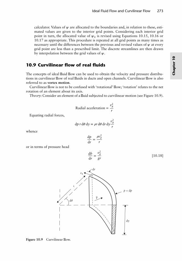
Ideal Fluid Flow and Curvilinear Flow 273
calculator. Values of 𝜓 are allocated to the boundaries and, in relation to these, esti-mated values are given to the interior grid points. Considering each interior gridpoint in turn, the allocated value of 𝜓0 is revised using Equations 10.15, 10.16 or10.17 as appropriate. This procedure is repeated at all grid points as many times asnecessary until the differences between the previous and revised values of 𝜓 at everygrid point are less than a prescribed limit. The discrete streamlines are then drawnby interpolation between the grid values of 𝜓 .
10.9 Curvilinear flow of real fluids
The concepts of ideal fluid flow can be used to obtain the velocity and pressure distribu-tions in curvilinear flow of real fluids in ducts and open channels. Curvilinear flow is alsoreferred to as vortex motion.
Curvilinear flow is not to be confused with ‘rotational’ flow; ‘rotation’ relates to the netrotation of an element about its axis.
Theory: Consider an element of a fluid subjected to curvilinear motion (see Figure 10.9).
Radial acceleration =v2𝜃
rEquating radial forces,
dp r d𝜃 dy = 𝜌r d𝜃 dr dyv2𝜃
rwhence
dp
dr=𝜌v2
𝜃
ror in terms of pressure head
dhdr
=v2𝜃
gr[10.18]
dy
dθp
rp + dp
drvθ
Figure 10.9 Curvilinear flow.
Ch
apte
r1
0
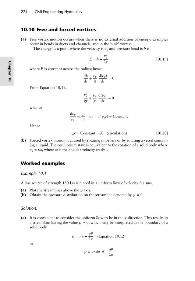
274 Civil Engineering Hydraulics
10.10 Free and forced vortices
(a) Free vortex motion occurs when there is no external addition of energy; examplesoccur in bends in ducts and channels, and in the ‘sink’ vortex.
The energy at a point where the velocity is v0 and pressure head is h is
E = h +v2𝜃
2g[10.19]
where E is constant across the radius; hence
dhdr
+v𝜃g
d(v𝜃)
dr= 0
From Equation 10.19,
v2𝜃
gr+
v𝜃g
d(v𝜃)
dr= 0
whence
dv𝜃v𝜃
= drr
or ln(v𝜃r) = Constant
Hence
v𝜃r = Constant = K (circulation) [10.20]
(b) Forced vortex motion is caused by rotating impellers or by rotating a vessel contain-ing a liquid. The equilibrium state is equivalent to the rotation of a solid body wherev𝜃 = r𝜔, where 𝜔 is the angular velocity (rad/s).
Worked examples
Example 10.1
A line source of strength 180 L/s is placed in a uniform flow of velocity 0.1 m/s.
(a) Plot the streamlines above the x-axis.(b) Obtain the pressure distribution on the streamline denoted by 𝜓 = 0.
Solution:
(a) It is convenient to consider the uniform flow to be in the x-direction. This results ina streamline having the value 𝜓 = 0, which may be interpreted as the boundary of asolid body.
𝜓 = uy +q𝜃2𝜋
(Equation 10.12)
or
𝜓 = ur sin 𝜃 +q𝜃2𝜋
Ch
apter
10
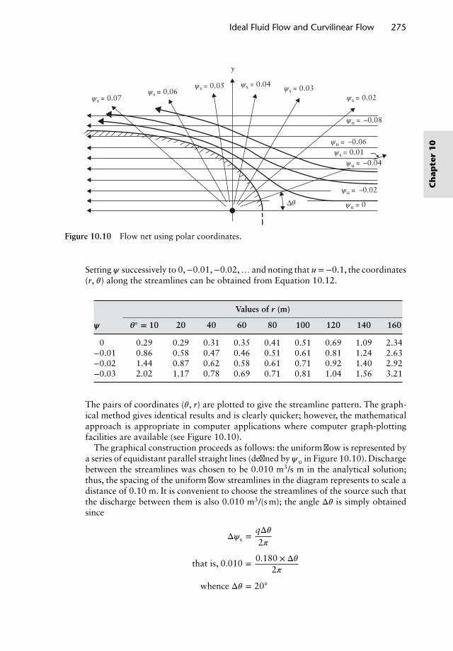
Ideal Fluid Flow and Curvilinear Flow 275
Δθ
ψs = 0.07ψs = 0.06
ψs = 0.05 ψs = 0.04 ψs = 0.03ψs = 0.02
ψu = –0.08
ψu = –0.06
ψu = –0.04
ψu = –0.02
ψs = 0.01
ψu = 0
y
Figure 10.10 Flow net using polar coordinates.
Setting𝜓 successively to 0,−0.01,−0.02,… and noting that u=−0.1, the coordinates(r, 𝜃) along the streamlines can be obtained from Equation 10.12.
Values of r (m)
𝝍 𝜽◦ = 10 20 40 60 80 100 120 140 160
0 0.29 0.29 0.31 0.35 0.41 0.51 0.69 1.09 2.34−0.01 0.86 0.58 0.47 0.46 0.51 0.61 0.81 1.24 2.63−0.02 1.44 0.87 0.62 0.58 0.61 0.71 0.92 1.40 2.92−0.03 2.02 1.17 0.78 0.69 0.71 0.81 1.04 1.56 3.21
The pairs of coordinates (𝜃, r) are plotted to give the streamline pattern. The graph-ical method gives identical results and is clearly quicker; however, the mathematicalapproach is appropriate in computer applications where computer graph-plottingfacilities are available (see Figure 10.10).
The graphical construction proceeds as follows: the uniform flow is represented bya series of equidistant parallel straight lines (defined by𝜓u in Figure 10.10). Dischargebetween the streamlines was chosen to be 0.010 m3/s m in the analytical solution;thus, the spacing of the uniform flow streamlines in the diagram represents to scale adistance of 0.10 m. It is convenient to choose the streamlines of the source such thatthe discharge between them is also 0.010 m3/(s m); the angle Δ𝜃 is simply obtainedsince
Δ𝜓s =qΔ𝜃2𝜋
that is, 0.010 = 0.180 × Δ𝜃2𝜋
whence Δ𝜃 = 20◦
Ch
apte
r1
0
276 Civil Engineering Hydraulics
At the points of intersection of the uniform flow and source streamlines, the indi-vidual stream functions are added algebraically and the resultant flow pattern isobtained by sketching the streamlines through points of equal resultant stream func-tion. The construction and final flow pattern are illustrated in Figure 10.10.
(b) The pressure distribution in the disturbed flow field at (r, 𝜃) is obtained from
pr,𝜃 − p0
𝜌g=
V20 − V2
r 𝜃
2g(i)
where V0 is the undisturbed velocity and Vr,𝜃 the velocity vector at (r, 𝜃).
Vr,𝜃 =√
v2r + v2
𝜃
vr =1r𝜕𝜓
𝜕𝜃(Equation 10.3)
= ur cos 𝜃r
+q
2𝜋r
v𝜃 = −𝜕𝜓𝜕r
(Equation 10.3)
= −u sin 𝜃
⇒ V2r,𝜃 = u2 + 2u cos 𝜃
q2𝜋r
+( q
2𝜋r
)2(ii)
Around the ‘body’ (𝜓 = 0),
ur sin 𝜃 +q𝜃2𝜋
= 0
i.e.q
2𝜋= −ur sin 𝜃
𝜃
Thus
V2r,𝜃 = u2
(1 − sin 2𝜃
𝜃+ sin2
𝜃
𝜃2
)
whence, from Equation (i), since V0 = u in this case
pr,𝜃 − p0
𝜌g= u2
2g𝜃
(sin 2𝜃 − sin2
𝜃
𝜃
)(iii)
Substitution of u = −0.1 m/s into Equation (iii) yields the pressure distribution for arange of 𝜃.
Example 10.2
A discharge of 7 m3/(s m) width flows in a rectangular channel. A vertical sluice gate situ-ated in the channel has an opening of 1.5 m. Cc = 0.62; Cv = 0.95. Assuming that down-stream conditions permit free flow under the gate, draw the streamline pattern.
Ch
apter
10
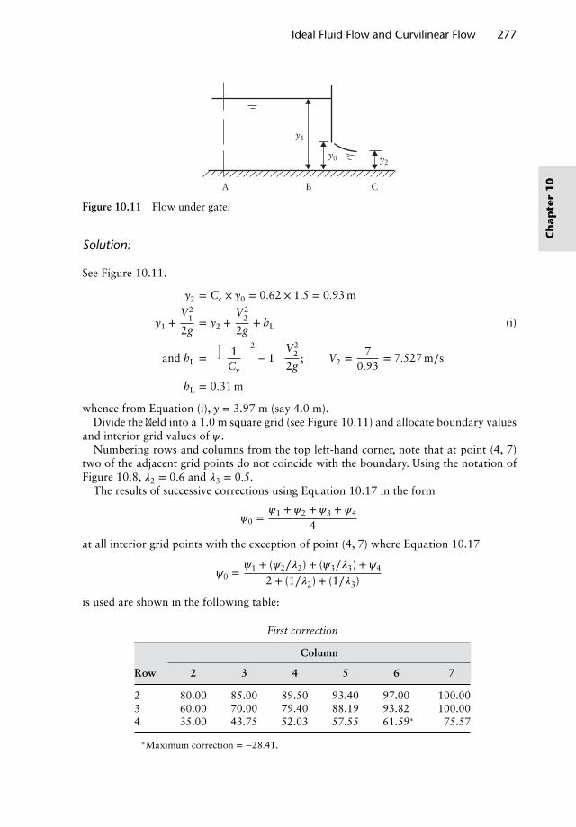
Ideal Fluid Flow and Curvilinear Flow 277
A B C
y1
y0 y2
Figure 10.11 Flow under gate.
Solution:
See Figure 10.11.
y2 = Cc × y0 = 0.62 × 1.5 = 0.93 m
y1 +V2
1
2g= y2 +
V22
2g+ hL (i)
and hL =
[(1
Cv
)2
− 1
]V2
2
2g; V2 = 7
0.93= 7.527 m∕s
hL = 0.31 m
whence from Equation (i), y = 3.97 m (say 4.0 m).Divide the field into a 1.0 m square grid (see Figure 10.11) and allocate boundary values
and interior grid values of 𝜓 .Numbering rows and columns from the top left-hand corner, note that at point (4, 7)
two of the adjacent grid points do not coincide with the boundary. Using the notation ofFigure 10.8, 𝜆2 = 0.6 and 𝜆3 = 0.5.
The results of successive corrections using Equation 10.17 in the form
𝜓0 =𝜓1 + 𝜓2 + 𝜓3 + 𝜓4
4
at all interior grid points with the exception of point (4, 7) where Equation 10.17
𝜓0 =𝜓1 + (𝜓2∕𝜆2) + (𝜓3∕𝜆3) + 𝜓4
2 + (1∕𝜆2) + (1∕𝜆3)
is used are shown in the following table:
First correction
Column
Row 2 3 4 5 6 7
2 80.00 85.00 89.50 93.40 97.00 100.003 60.00 70.00 79.40 88.19 93.82 100.004 35.00 43.75 52.03 57.55 61.59∗ 75.57
∗Maximum correction = −28.41.
Ch
apte
r1
0
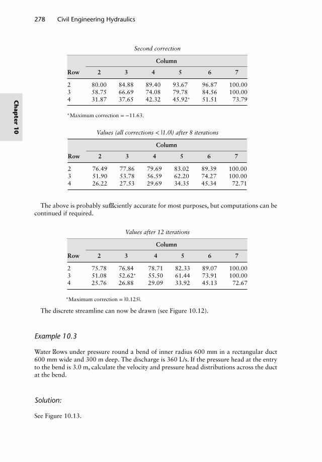
278 Civil Engineering Hydraulics
Second correction
Column
Row 2 3 4 5 6 7
2 80.00 84.88 89.40 93.67 96.87 100.003 58.75 66.69 74.08 79.78 84.56 100.004 31.87 37.65 42.32 45.92∗ 51.51 73.79
∗Maximum correction = −11.63.
Values (all corrections < |1.0|) after 8 iterations
Column
Row 2 3 4 5 6 7
2 76.49 77.86 79.69 83.02 89.39 100.003 51.90 53.78 56.59 62.20 74.27 100.004 26.22 27.53 29.69 34.35 45.34 72.71
The above is probably sufficiently accurate for most purposes, but computations can becontinued if required.
Values after 12 iterations
Column
Row 2 3 4 5 6 7
2 75.78 76.84 78.71 82.33 89.07 100.003 51.08 52.62∗ 55.50 61.44 73.91 100.004 25.76 26.88 29.09 33.92 45.13 72.67
∗Maximum correction = |0.125|.
The discrete streamline can now be drawn (see Figure 10.12).
Example 10.3
Water flows under pressure round a bend of inner radius 600 mm in a rectangular duct600 mm wide and 300 m deep. The discharge is 360 L/s. If the pressure head at the entryto the bend is 3.0 m, calculate the velocity and pressure head distributions across the ductat the bend.
Solution:
See Figure 10.13.
Ch
apter
10
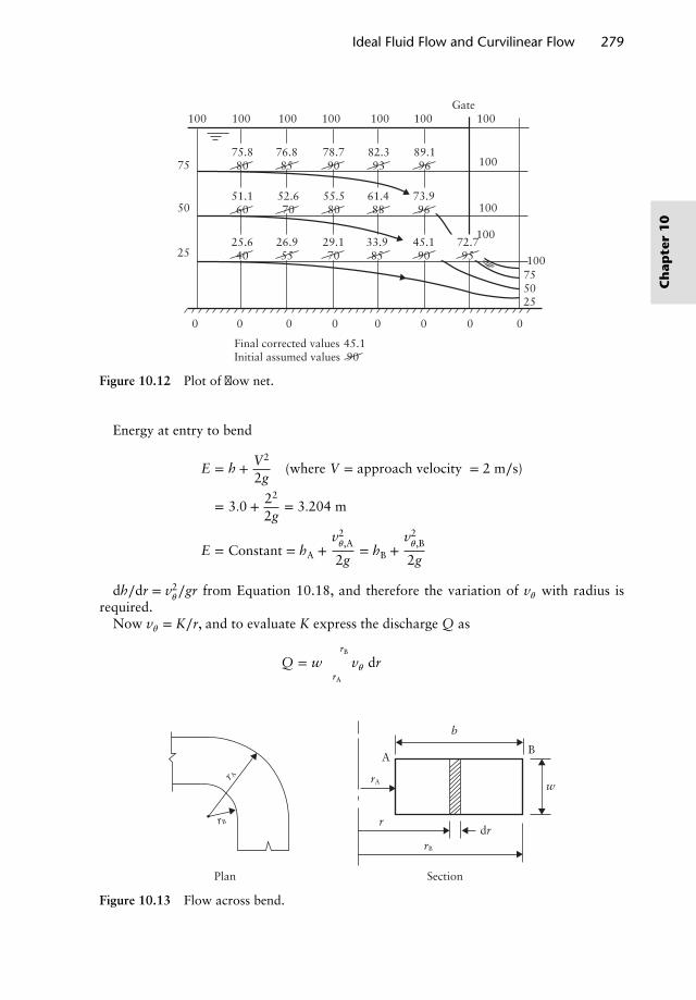
Ideal Fluid Flow and Curvilinear Flow 279
100 100
75.880
51.160
25.640
26.955
29.170
33.985
45.190
72.795
52.670
55.580
61.488
73.996
76.885
78.790
82.393
89.196
100 100 100 100Gate
100
100
100
100
100755025
Final corrected values 45.1Initial assumed values 90
00000000
25
50
75
Figure 10.12 Plot of flow net.
Energy at entry to bend
E = h + V2
2g(where V = approach velocity = 2 m∕s)
= 3.0 + 22
2g= 3.204 m
E = Constant = hA +v2𝜃,A
2g= hB +
v2𝜃,B
2g
dh∕dr = v2𝜃∕gr from Equation 10.18, and therefore the variation of v𝜃 with radius is
required.Now v𝜃 = K∕r, and to evaluate K express the discharge Q as
Q = w∫rB
rA
v𝜃 dr
r
AB
b
SectionPlan
w
rB
rAr A
rB
dr
Figure 10.13 Flow across bend.
Ch
apte
r1
0
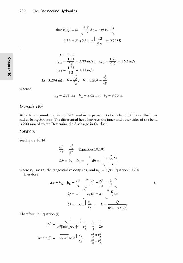
280 Civil Engineering Hydraulics
that is, Q = w∫rB
rA
Kr
dr = Kw ln(
rB
rA
)
0.36 = K × 0.3 × ln(
1.20.6
)= 0.208K
or
K = 1.73
v𝜃,A = 1.730.6
= 2.88 m∕s; v𝜃,C = 1.730.9
= 1.92 m∕s
v𝜃,B = 1.731.2
= 1.44 m∕s
E(=3.204 m) = h +v2𝜃
2g; h = 3.204 −
v2𝜃
2g
whence
hA = 2.78 m; hC = 3.02 m; hB = 3.10 m
Example 10.4
Water flows round a horizontal 90◦ bend in a square duct of side length 200 mm, the innerradius being 300 mm. The differential head between the inner and outer sides of the bendis 200 mm of water. Determine the discharge in the duct.
Solution:
See Figure 10.14.
dhdr
=V2𝜃
gr(Equation 10.18)
Δh = hA − hB = ∫B
Adh = ∫
rB
rA
v2𝜃,r dr
gr
where v𝜃,r means the tangential velocity at r, and v𝜃,r = K∕r (Equation 10.20).Therefore
Δh = hA − hB = K2
g ∫rB
rA
drr3
= K2
2g
[− 1
r2
]rB
rA
(i)
Q = w ∫rB
rA
v𝜃 dr = w ∫rB
rA
Kr
dr
Q = wK ln(
rB
rA
); K =
Q
w ln(rB∕rA
)Therefore, in Equation (i)
Δh =Q2
w2[ln(rB∕rA)]2
(1r2A
− 1r2B
)12g
where Q =√
2gΔh w ln(
rB
rA
)√√√√ r2B × r2
A
r2B − r2
A
Ch
apter
10
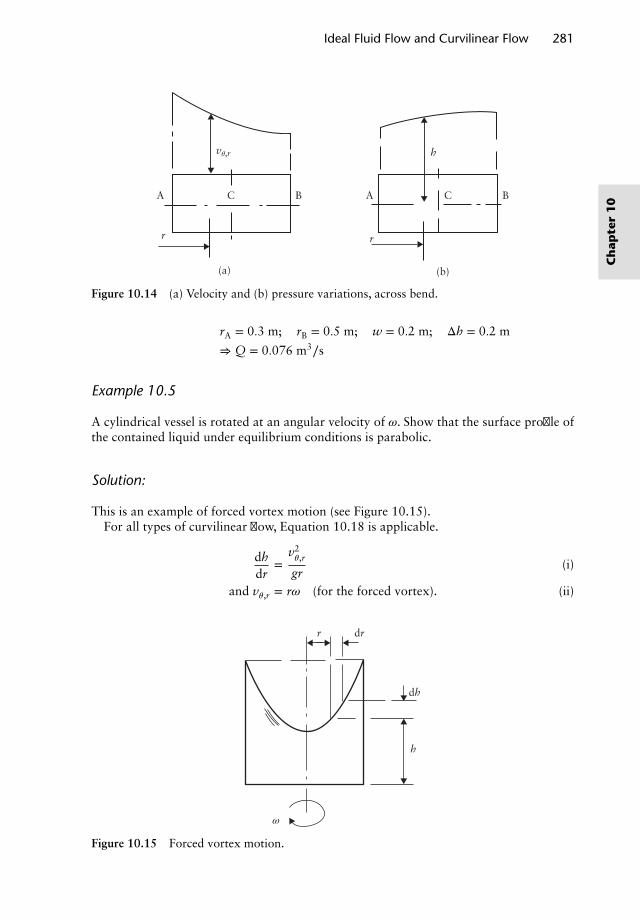
Ideal Fluid Flow and Curvilinear Flow 281
AA
r
h
r
C
(a) (b)
vθ,r
C BB
Figure 10.14 (a) Velocity and (b) pressure variations, across bend.
rA = 0.3 m; rB = 0.5 m; w = 0.2 m; Δh = 0.2 m
⇒ Q = 0.076 m3∕s
Example 10.5
A cylindrical vessel is rotated at an angular velocity of 𝜔. Show that the surface profile ofthe contained liquid under equilibrium conditions is parabolic.
Solution:
This is an example of forced vortex motion (see Figure 10.15).For all types of curvilinear flow, Equation 10.18 is applicable.
dhdr
=v2𝜃,r
gr(i)
and v𝜃,r = r𝜔 (for the forced vortex). (ii)
r dr
dh
h
ω
Figure 10.15 Forced vortex motion.
Ch
apte
r1
0
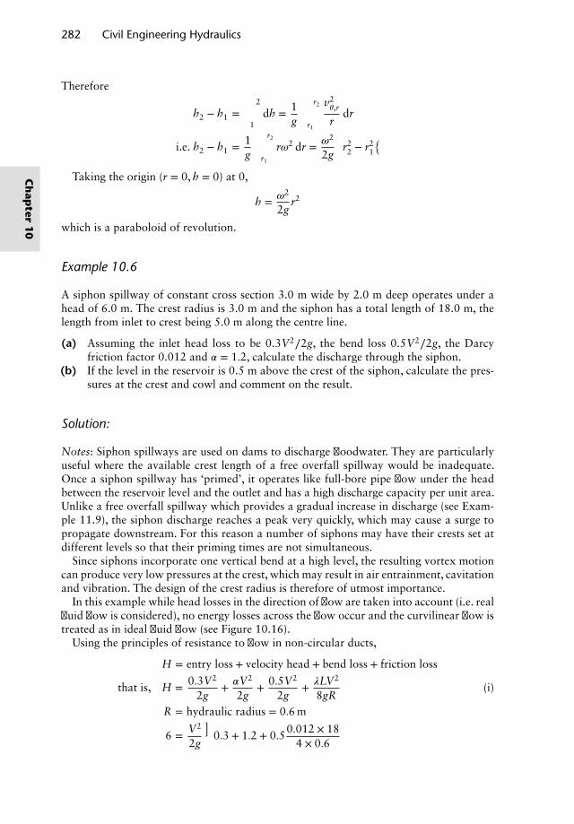
282 Civil Engineering Hydraulics
Therefore
h2 − h1 = ∫2
1dh = 1
g ∫r2
r1
v2𝜃,r
rdr
i.e. h2 − h1 = 1g ∫
r2
r1
r𝜔2 dr = 𝜔2
2g
(r22 − r2
1
)Taking the origin (r = 0, h = 0) at 0,
h = 𝜔2
2gr2
which is a paraboloid of revolution.
Example 10.6
A siphon spillway of constant cross section 3.0 m wide by 2.0 m deep operates under ahead of 6.0 m. The crest radius is 3.0 m and the siphon has a total length of 18.0 m, thelength from inlet to crest being 5.0 m along the centre line.
(a) Assuming the inlet head loss to be 0.3V2∕2g, the bend loss 0.5V2∕2g, the Darcyfriction factor 0.012 and 𝛼 = 1.2, calculate the discharge through the siphon.
(b) If the level in the reservoir is 0.5 m above the crest of the siphon, calculate the pres-sures at the crest and cowl and comment on the result.
Solution:
Notes: Siphon spillways are used on dams to discharge floodwater. They are particularlyuseful where the available crest length of a free overfall spillway would be inadequate.Once a siphon spillway has ‘primed’, it operates like full-bore pipe flow under the headbetween the reservoir level and the outlet and has a high discharge capacity per unit area.Unlike a free overfall spillway which provides a gradual increase in discharge (see Exam-ple 11.9), the siphon discharge reaches a peak very quickly, which may cause a surge topropagate downstream. For this reason a number of siphons may have their crests set atdifferent levels so that their priming times are not simultaneous.
Since siphons incorporate one vertical bend at a high level, the resulting vortex motioncan produce very low pressures at the crest, which may result in air entrainment, cavitationand vibration. The design of the crest radius is therefore of utmost importance.
In this example while head losses in the direction of flow are taken into account (i.e. realfluid flow is considered), no energy losses across the flow occur and the curvilinear flow istreated as in ideal fluid flow (see Figure 10.16).
Using the principles of resistance to flow in non-circular ducts,
H = entry loss + velocity head + bend loss + friction loss
that is, H = 0.3V2
2g+ 𝛼V2
2g+ 0.5V2
2g+ 𝜆LV2
8gR(i)
R = hydraulic radius = 0.6 m
6 = V2
2g
(0.3 + 1.2 + 0.50.012 × 18
4 × 0.6
)
Ch
apter
10
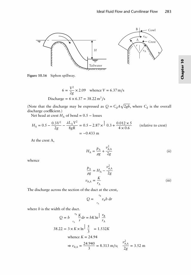
Ideal Fluid Flow and Curvilinear Flow 283
H
r
rA
vθ,r
Tailwater
Crest
B Cowl
A
Figure 10.16 Siphon spillway.
6 = V2
2g× 2.09 whence V = 6.37 m∕s
Discharge = 6 × 6.37 = 38.22 m3∕s
(Note that the discharge may be expressed as Q = CdA√
2gh, where Cd is the overalldischarge coefficient.)
Net head at crest HA of bend = 0.5 − losses
HA = 0.5 − 0.3V2
2g−𝜆LAV2
8gR= 0.5 − 2.87 ×
(0.3 + 0.012 × 5
4 × 0.6
)(relative to crest)
= −0.433 m
At the crest A,
HA =pA
𝜌g+
v2𝜃,A
2g(ii)
whence
pA
𝜌g= HA −
v2𝜃,A
2g
v𝜃,A = KrA
(iii)
The discharge across the section of the duct at the crest,
Q = ∫rB
rA
v𝜃b dr
where b is the width of the duct.
Q = b∫rB
rA
Kr
dr = bK ln(
rB
rA
)
38.22 = 3 × K × ln(
53
)= 1.532K
whence K = 24.94
⇒ v𝜃,A = 24.9403
= 8.313 m∕s;v2𝜃,A
2g= 3.52 m
Ch
apte
r1
0
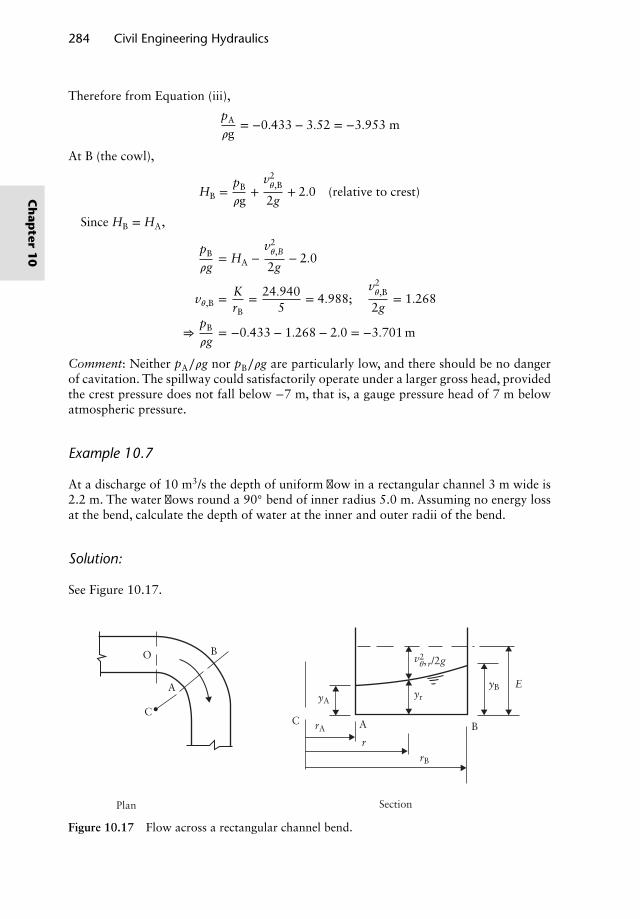
284 Civil Engineering Hydraulics
Therefore from Equation (iii),
pA
𝜌g= −0.433 − 3.52 = −3.953 m
At B (the cowl),
HB =pB
𝜌g+
v2𝜃,B
2g+ 2.0 (relative to crest)
Since HB = HA,
pB
𝜌g= HA −
v2𝜃,B
2g− 2.0
v𝜃,B = KrB
= 24.9405
= 4.988;v2𝜃,B
2g= 1.268
⇒pB
𝜌g= −0.433 − 1.268 − 2.0 = −3.701 m
Comment: Neither pA∕𝜌g nor pB∕𝜌g are particularly low, and there should be no dangerof cavitation. The spillway could satisfactorily operate under a larger gross head, providedthe crest pressure does not fall below −7 m, that is, a gauge pressure head of 7 m belowatmospheric pressure.
Example 10.7
At a discharge of 10 m3/s the depth of uniform flow in a rectangular channel 3 m wide is2.2 m. The water flows round a 90◦ bend of inner radius 5.0 m. Assuming no energy lossat the bend, calculate the depth of water at the inner and outer radii of the bend.
Solution:
See Figure 10.17.
B
B
E
O
A
A
SectionPlan
CC
yA
rA
yr
v2θ, r/2g
yB
rB
r
Figure 10.17 Flow across a rectangular channel bend.
Ch
apter
10
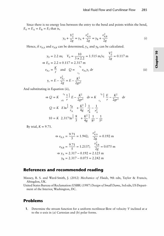
Ideal Fluid Flow and Curvilinear Flow 285
Since there is no energy loss between the entry to the bend and points within the bend,E0 = EA = EB = E; that is,
y0 +V2
0
2g= yA +
v2𝜃,A
2g= yB +
v2𝜃,B
2g(i)
Hence, if v𝜃,A and v𝜃,B can be determined, yA and yB can be calculated.
y0 = 2.2 m; V0 = 103 × 2.2
= 1.515 m∕s;V2
0
2g= 0.117 m
⇒ E0 = 2.2 + 0.117 = 2.317 m
v𝜃,r =Kr
and Q = ∫rB
rA
v𝜃,ryr dr (ii)
yr = E −v2𝜃,r
2g= E − K2
2gr2
And substituting in Equation (ii),
⇒ Q = K∫rB
rA
1r
(E − K2
2gr2
)dr = K∫
rB
rA
(Er− K2
2gr3
)dr
Q = K
[E ln
(rB
rA
)+ K2
4g
(1r2B
− 1r2A
)]
10 = K[2.317 ln
(85
)+ K2
4g
(182
− 152
)]
By trial, K = 9.71.
⇒ v𝜃,A = 9.715
= 1.942;v2𝜃,A
2g= 0.192 m
v𝜃,B = 9.715
= 1.2137;v2𝜃,B
2g= 0.075 m
⇒ yA = 2.317 − 0.192 = 2.125 m
yB = 2.317 − 0.075 = 2.242 m
References and recommended reading
Massey, B. S. and Ward-Smith, J. (2012) Mechanics of Fluids, 9th edn, Taylor & Francis,Abingdon, UK.
United States Bureau of Reclamation (USBR) (1987) Design of Small Dams, 3rd edn, US Depart-ment of the Interior, Washington, DC.
Problems
1. Determine the stream function for a uniform rectilinear flow of velocity V inclined at 𝛼to the x-axis in (a) Cartesian and (b) polar forms.
Ch
apte
r1
0
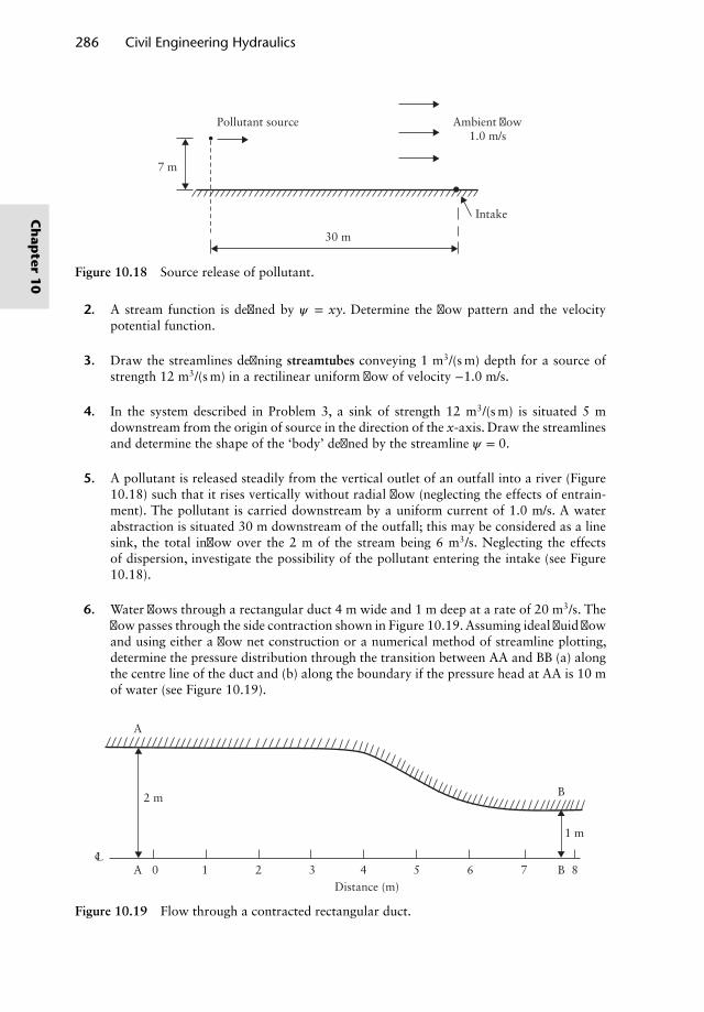
286 Civil Engineering Hydraulics
Ambient flowPollutant source1.0 m/s
Intake
30 m
7 m
Figure 10.18 Source release of pollutant.
2. A stream function is defined by 𝜓 = xy. Determine the flow pattern and the velocitypotential function.
3. Draw the streamlines defining streamtubes conveying 1 m3/(s m) depth for a source ofstrength 12 m3/(s m) in a rectilinear uniform flow of velocity −1.0 m/s.
4. In the system described in Problem 3, a sink of strength 12 m3/(s m) is situated 5 mdownstream from the origin of source in the direction of the x-axis. Draw the streamlinesand determine the shape of the ‘body’ defined by the streamline 𝜓 = 0.
5. A pollutant is released steadily from the vertical outlet of an outfall into a river (Figure10.18) such that it rises vertically without radial flow (neglecting the effects of entrain-ment). The pollutant is carried downstream by a uniform current of 1.0 m/s. A waterabstraction is situated 30 m downstream of the outfall; this may be considered as a linesink, the total inflow over the 2 m of the stream being 6 m3/s. Neglecting the effectsof dispersion, investigate the possibility of the pollutant entering the intake (see Figure10.18).
6. Water flows through a rectangular duct 4 m wide and 1 m deep at a rate of 20 m3/s. Theflow passes through the side contraction shown in Figure 10.19. Assuming ideal fluid flowand using either a flow net construction or a numerical method of streamline plotting,determine the pressure distribution through the transition between AA and BB (a) alongthe centre line of the duct and (b) along the boundary if the pressure head at AA is 10 mof water (see Figure 10.19).
ALc
A
3210Distance (m)
2 m
87654 B
B
1 m
Figure 10.19 Flow through a contracted rectangular duct.
Ch
apter
10
Ideal Fluid Flow and Curvilinear Flow 287
7. A discharge of 6 m3/s per unit width approaches a vertical sluice gate in a rectangularchannel at a depth of 4 m. The vertical gate opening is 1.5 m and Cd = 0.6. Assumingthat downstream conditions do not affect the natural flow through the gate opening,verify that the flow through the opening is supercritical, draw the streamline pattern anddetermine the pressure distribution and force per unit width on the gate. Compare thevalue of force obtained with that obtained using the momentum equation.
8. Water flows under pressure in a horizontal rectangular duct of width b and depth w.The pressure head difference across the duct, at a horizontal bend of radius R to thecentre line, is h. Show that if R = 1.5 b, the discharge is obtained from the expression
Q = 3.545 w b√
h.
9. Water flows round a horizontal 90◦ bend in a square duct of side length 200 mm, theinner radius being 400 mm. The differential head between the inner and outer sides ofthe bend is 150 mm of water. Determine the discharge in the duct.
10. The depth of uniform flow of water in a rectangular channel 5 m wide conveying 40 m3/sis 2.5 m. The water flows round a 90◦ bend of inner radius 10 m. Assuming no energyloss through the bend, determine the depth of water at the inner and outer radii of thebend at the discharge of 150 m3/s.
11. A proposed siphon spillway is of uniform rectangular sections 5 m wide and 3 m deep.The crest radius is 3 m, and the length of the approach to the crest along the centre line is7 m. The overall discharge coefficient is 0.65; the entry head loss = 0.2V2∕2g, where V isthe mean velocity; and the Darcy friction factor is 0.015. Determine the discharge whenthe siphon operates under a head of 6 m with the upstream water level 0.5 m above thecrest, and determine the pressure heads at the crest and cowl.
12. Water discharges from a tank through a circular orifice 25 mm in diameter in the base.The discharge coefficient under conditions of radial flow towards the orifice in the tankis 0.6. A free vortex forms when water is discharging under a head of 150 mm; at ahorizontal distance of 10 mm from the centre line of the orifice, the water surface is50 mm below the top water level. Determine the discharge through the orifice.
13. A cylindrical vessel 0.61 m in diameter and 0.97 m in depth, open at the top, is rotatedabout a vertical axis at 105 rev/min. If the vessel was originally full of water, how muchwater will remain under equilibrium conditions?
Ch
apte
r1
0

Chapter 11Gradually Varied UnsteadyFlow from Reservoirs
11.1 Discharge between reservoirs under varying head
Figure 11.1 shows two reservoirs, of constant area, interconnected by a pipeline throughwhich water transfer occurs under gravity. Reservoir A receives an inflow I1, while a dis-charge Q2 is withdrawn from B; I1 and Q2 may be time variant.
In the general case the head h and hence the transfer discharge will vary with time, andthe object is to obtain a differential equation describing the rate of variation of head withtime, dh∕dt. The corresponding rate of change of discharge is considered to be sufficientlysmall so that the steady-state discharge–head relationship for the pipeline flow may beapplied at any instantaneous head; compressibility effects are also neglected. Such unsteadyflow situations are therefore sometimes referred to as ‘quasi-steady’ flow.
Let h be the gross head at any instant, Δh1 the change in level in A during a small timeinterval Δt and Δh2 the change in level in B in time Δt; then
change in total head = Δh = Δh1 − Δh2 [11.1]
Continuity equation for A: I − Q1 = A1Δh1
t[11.2]
Continuity equation for B: Q1 − Q2 = A2Δh2
t[11.3]
Note that Q1 is the discharge in the pipeline and hence is the inflow rate into B.From the steady-state head–discharge relationship for the pipeline,
h =(
Km + 𝜆LD
) Q21
2gA2p
where Ap is the area of pipe and Km the minor loss coefficient. Whence
Q1 = Kh1∕2 [11.4]
Nalluri & Featherstone’s Civil Engineering Hydraulics: Essential Theory with Worked Examples,Sixth Edition. Martin Marriott.© 2016 John Wiley & Sons, Ltd. Published 2016 by John Wiley & Sons, Ltd.Companion Website: www.wiley.com/go/Marriott
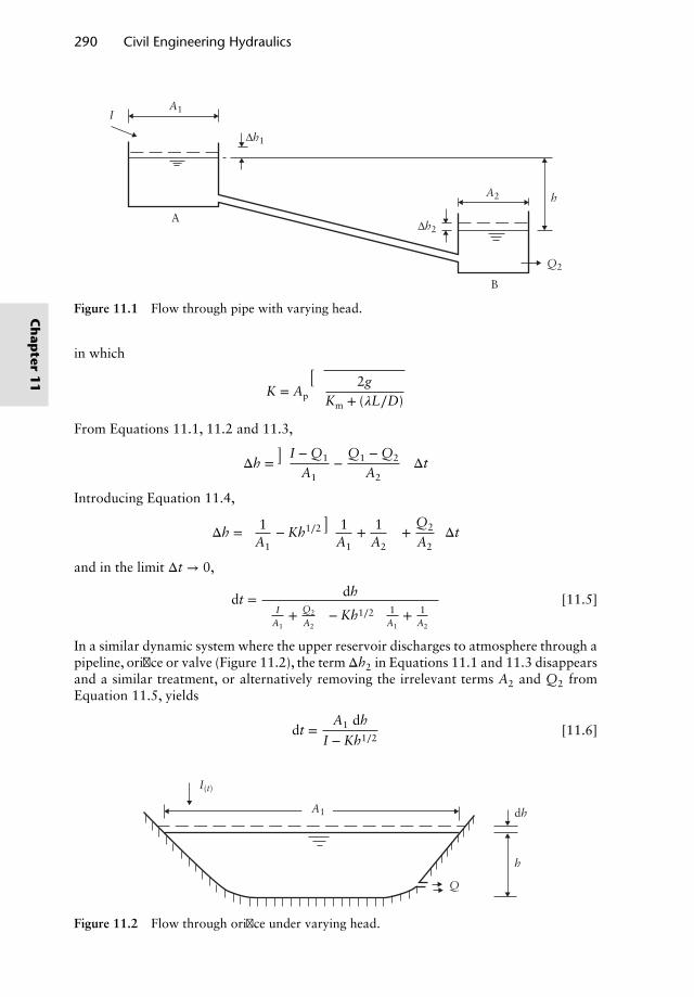
290 Civil Engineering Hydraulics
A1
A2
A
B
Q2
h
Δh1
Δh2
I
Figure 11.1 Flow through pipe with varying head.
in which
K = Ap
√2g
Km + (𝜆L∕D)
From Equations 11.1, 11.2 and 11.3,
Δh =(
I − Q1
A1−
Q1 − Q2
A2
)Δt
Introducing Equation 11.4,
Δh =[
1A1
− Kh1∕2(
1A1
+ 1A2
)+
Q2
A2
]Δt
and in the limit Δt → 0,
dt = dh(I
A1+ Q2
A2
)− Kh1∕2
(1
A1+ 1
A2
) [11.5]
In a similar dynamic system where the upper reservoir discharges to atmosphere through apipeline, orifice or valve (Figure 11.2), the term Δh2 in Equations 11.1 and 11.3 disappearsand a similar treatment, or alternatively removing the irrelevant terms A2 and Q2 fromEquation 11.5, yields
dt =A1 dh
I − Kh1∕2[11.6]
I(t)
A1
Q
h
dh
Figure 11.2 Flow through orifice under varying head.
Ch
apter
11
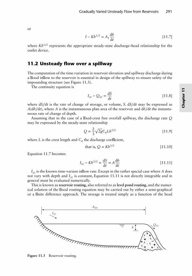
Gradually Varied Unsteady Flow from Reservoirs 291
or
I − Kh1∕2 = A1dhdt
[11.7]
where Kh1∕2 represents the appropriate steady-state discharge–head relationship for theoutlet device.
11.2 Unsteady flow over a spillway
The computation of the time variation in reservoir elevation and spillway discharge duringa flood inflow to the reservoir is essential in design of the spillway to ensure safety of theimpounding structure (see Figure 11.3).
The continuity equation is
I(t) − Q(t) =dSdt
[11.8]
where dS∕dt is the rate of change of storage, or volume, S. dS∕dt may be expressed asA(dh∕dt), where A is the instantaneous plan area of the reservoir and dh∕dt the instanta-neous rate of change of depth.
Assuming that in the case of a fixed-crest free overfall spillway, the discharge rate Qmay be expressed by the steady-state relationship
Q = 23
√2gCdLh3∕2 [11.9]
where L is the crest length and Cd the discharge coefficient,
that is, Q = Kh3∕2 [11.10]
Equation 11.7 becomes
I(t) − Kh3∕2 = dSdt
= Adhdt
[11.11]
I(t) is the known time-variant inflow rate. Except in the rather special case where A doesnot vary with depth and I(t) is constant, Equation 11.11 is not directly integrable and ingeneral must be evaluated numerically.
This is known as reservoir routing, also referred to as level pond routing, and the numer-ical solution of the flood routing equation may be carried out by either a semi-graphicalor a finite difference approach. The storage is treated simply as a function of the head
I(t)
A(h)
Q(t)h
Figure 11.3 Reservoir routing.
Ch
apte
r1
1
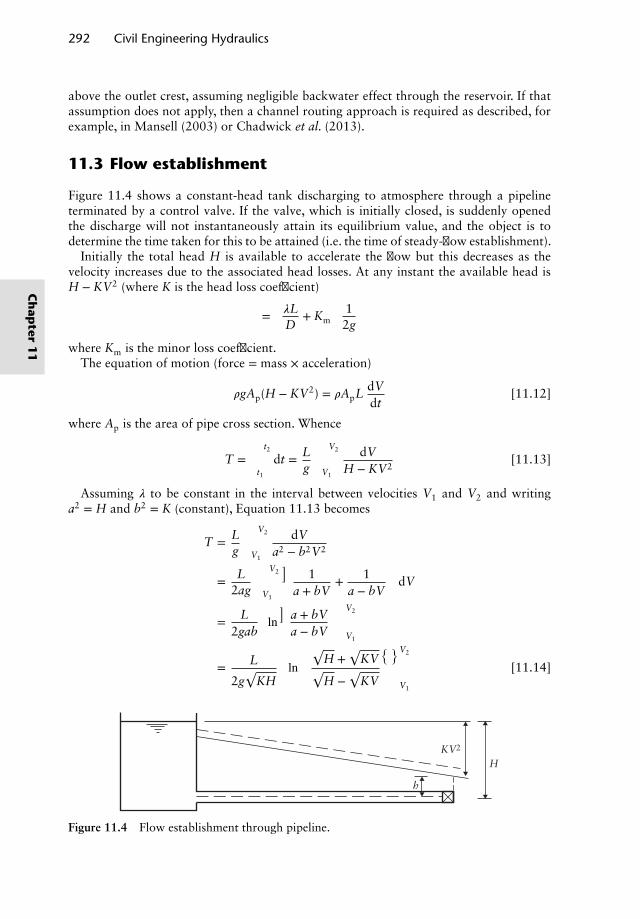
292 Civil Engineering Hydraulics
above the outlet crest, assuming negligible backwater effect through the reservoir. If thatassumption does not apply, then a channel routing approach is required as described, forexample, in Mansell (2003) or Chadwick et al. (2013).
11.3 Flow establishment
Figure 11.4 shows a constant-head tank discharging to atmosphere through a pipelineterminated by a control valve. If the valve, which is initially closed, is suddenly openedthe discharge will not instantaneously attain its equilibrium value, and the object is todetermine the time taken for this to be attained (i.e. the time of steady-flow establishment).
Initially the total head H is available to accelerate the flow but this decreases as thevelocity increases due to the associated head losses. At any instant the available head isH − KV2 (where K is the head loss coefficient)
=(𝜆LD
+ Km
) 12g
where Km is the minor loss coefficient.The equation of motion (force = mass × acceleration)
𝜌gAp(H − KV2) = 𝜌ApLdVdt
[11.12]
where Ap is the area of pipe cross section. Whence
T = ∫t2
t1
dt = Lg ∫
V2
V1
dVH − KV2
[11.13]
Assuming 𝜆 to be constant in the interval between velocities V1 and V2 and writinga2 = H and b2 = K (constant), Equation 11.13 becomes
T = Lg ∫
V2
V1
dVa2 − b2V2
= L2ag ∫
V2
V1
(1
a + bV+ 1
a − bV
)dV
= L2gab
[ln(
a + bVa − bV
)]V2
V1
= L
2g√
KH
[ln
(√H +
√KV√
H −√
KV
)]V2
V1
[11.14]
KV2
h
H
Figure 11.4 Flow establishment through pipeline.
Ch
apter
11
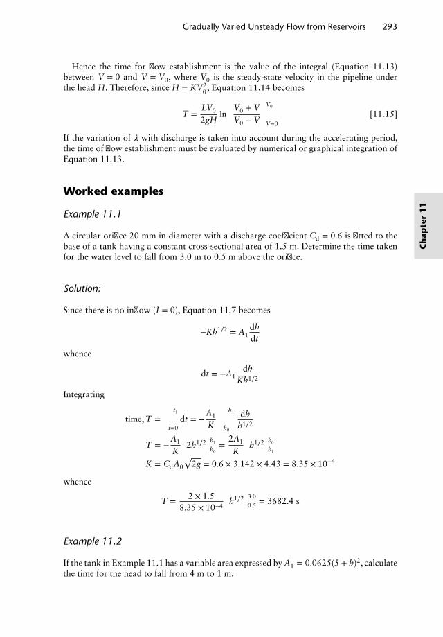
Gradually Varied Unsteady Flow from Reservoirs 293
Hence the time for flow establishment is the value of the integral (Equation 11.13)between V = 0 and V = V0, where V0 is the steady-state velocity in the pipeline underthe head H. Therefore, since H = KV2
0 , Equation 11.14 becomes
T =LV0
2gHln[
V0 + VV0 − V
]V0
V=0[11.15]
If the variation of 𝜆 with discharge is taken into account during the accelerating period,the time of flow establishment must be evaluated by numerical or graphical integration ofEquation 11.13.
Worked examples
Example 11.1
A circular orifice 20 mm in diameter with a discharge coefficient Cd = 0.6 is fitted to thebase of a tank having a constant cross-sectional area of 1.5 m. Determine the time takenfor the water level to fall from 3.0 m to 0.5 m above the orifice.
Solution:
Since there is no inflow (I = 0), Equation 11.7 becomes
−Kh1∕2 = A1dhdt
whence
dt = −A1dh
Kh1∕2
Integrating
time, T = ∫t1
t=0dt = −
A1
K ∫h1
h0
dhh1∕2
T = −A1
K
[2h1∕2]h1
h0=
2A1
K
[h1∕2]h0
h1
K = CdA0
√2g = 0.6 × 3.142 × 4.43 = 8.35 × 10⁻⁴
whence
T = 2 × 1.58.35 × 10−4
[h1∕2]3.0
0.5 = 3682.4 s
Example 11.2
If the tank in Example 11.1 has a variable area expressed by A1 = 0.0625(5 + h)2, calculatethe time for the head to fall from 4 m to 1 m.
Ch
apte
r1
1
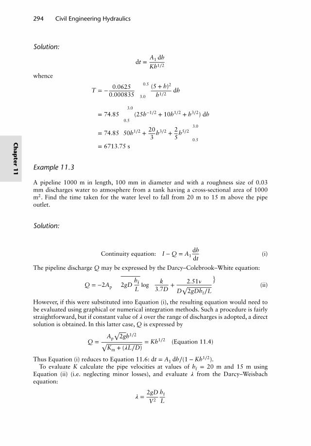
294 Civil Engineering Hydraulics
Solution:
dt =A1 dh
Kh1∕2
whence
T = − 0.06250.000835 ∫
0.5
3.0
(5 + h)2
h1∕2dh
= 74.85∫3.0
0.5(25h−1∕2 + 10h1∕2 + h3∕2) dh
= 74.85[50h1∕2 + 20
3h3∕2 + 2
5h5∕2
]3.0
0.5
= 6713.75 s
Example 11.3
A pipeline 1000 m in length, 100 mm in diameter and with a roughness size of 0.03mm discharges water to atmosphere from a tank having a cross-sectional area of 1000m2. Find the time taken for the water level to fall from 20 m to 15 m above the pipeoutlet.
Solution:
Continuity equation: I − Q = A1dhdt
(i)
The pipeline discharge Q may be expressed by the Darcy–Colebrook–White equation:
Q = −2Ap
√2gD
hf
Llog
[k
3.7D+ 2.51𝜈
D√
2gDhf∕L
](ii)
However, if this were substituted into Equation (i), the resulting equation would need tobe evaluated using graphical or numerical integration methods. Such a procedure is fairlystraightforward, but if constant value of 𝜆 over the range of discharges is adopted, a directsolution is obtained. In this latter case, Q is expressed by
Q =Ap
√2gh1∕2√
Km + (𝜆L∕D)= Kh1∕2 (Equation 11.4)
Thus Equation (i) reduces to Equation 11.6: dt = A1 dh∕(1 − Kh1∕2).To evaluate K calculate the pipe velocities at values of hf = 20 m and 15 m using
Equation (ii) (i.e. neglecting minor losses), and evaluate 𝜆 from the Darcy–Weisbachequation:
𝜆 =2gD
V2
hf
L
Ch
apter
11
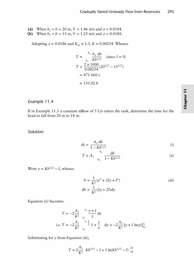
Gradually Varied Unsteady Flow from Reservoirs 295
(a) When hf = h = 20 m, V = 1.46 m/s and 𝜆 = 0.0184.(b) When hf = h = 15 m, V = 1.25 m/s and 𝜆 = 0.0188.
Adopting 𝜆 = 0.0186 and Km = 1.5, K = 0.00254. Whence
T = ∫h2
h1
A1 dh
Kh1∕2(since I = 0)
T = 2 × 10000.00254
(201∕2 − 151∕2)
= 471 660 s
= 131.02 h
Example 11.4
If in Example 11.3 a constant inflow of 5 L/s enters the tank, determine the time for thehead to fall from 20 m to 18 m.
Solution:
dt =A1 dh
1 − Kh1∕2(i)
T = A1 ∫h1
h0
dhI − Kh1∕2
(ii)
Write y = Kh1∕2 − I, whence
h = 1K2
(y2 + 2Iy + I2) (iii)
dh = 1K2
(2y + 2I)dy
Equation (ii) becomes
T = −2A1
K2 ∫y1
y0
y + Iy
dy
i.e. T = −2A1
K2 ∫y1
y0
(1 + I
y
)dy = −2
A1
K2[y + I ln(y)]y1
y0
Substituting for y from Equation (iii),
T = 2A1
K2
[Kh1∕2 − I + I ln(Kh1∕2 − I)
]20
18
Ch
apte
r1
1
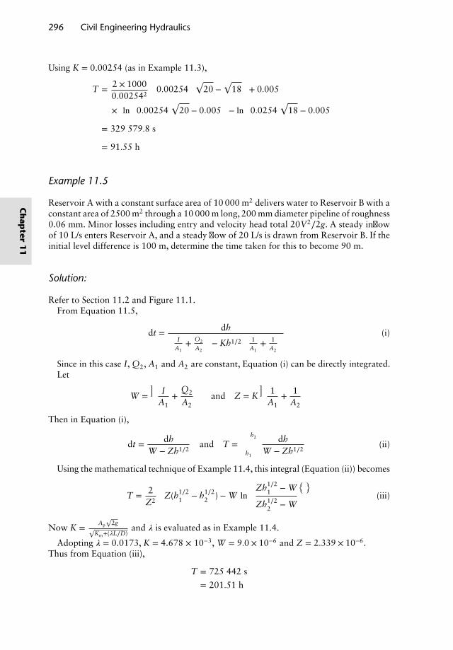
296 Civil Engineering Hydraulics
Using K = 0.00254 (as in Example 11.3),
T = 2 × 10000.002542
{0.00254
(√20 −
√18
)+ 0.005
×[ln(
0.00254√
20 − 0.005)− ln
(0.0254
√18 − 0.005
)]}= 329 579.8 s
= 91.55 h
Example 11.5
Reservoir A with a constant surface area of 10 000 m2 delivers water to Reservoir B with aconstant area of 2500 m2 through a 10 000 m long, 200 mm diameter pipeline of roughness0.06 mm. Minor losses including entry and velocity head total 20V2∕2g. A steady inflowof 10 L/s enters Reservoir A, and a steady flow of 20 L/s is drawn from Reservoir B. If theinitial level difference is 100 m, determine the time taken for this to become 90 m.
Solution:
Refer to Section 11.2 and Figure 11.1.From Equation 11.5,
dt = dh(I
A1+ O2
A2
)− Kh1∕2
(1
A1+ 1
A2
) (i)
Since in this case I, Q2, A1 and A2 are constant, Equation (i) can be directly integrated.Let
W =(
IA1
+Q2
A2
)and Z = K
(1
A1+ 1
A2
)
Then in Equation (i),
dt = dhW − Zh1∕2
and T = ∫h2
h1
dhW − Zh1∕2
(ii)
Using the mathematical technique of Example 11.4, this integral (Equation (ii)) becomes
T = 2Z2
[Z(h1∕2
1 − h1∕22 ) − W ln
(Zh1∕2
1 − W
Zh1∕22 − W
)](iii)
Now K = Ap
√2g√
Km+(𝜆L∕D)and 𝜆 is evaluated as in Example 11.4.
Adopting 𝜆 = 0.0173, K = 4.678 × 10⁻³, W = 9.0 × 10⁻⁶ and Z = 2.339 × 10⁻⁶.Thus from Equation (iii),
T = 725 442 s
= 201.51 h
Ch
apter
11
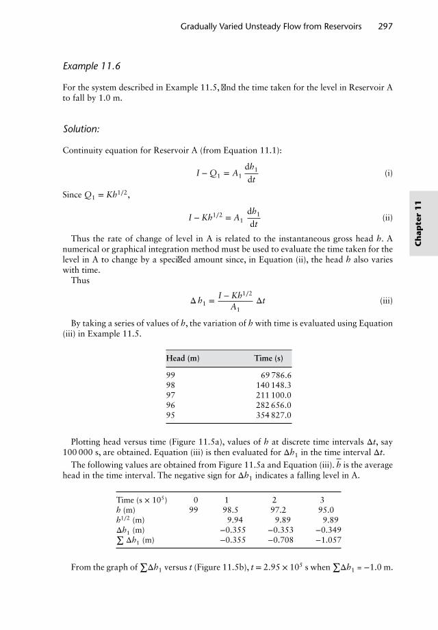
Gradually Varied Unsteady Flow from Reservoirs 297
Example 11.6
For the system described in Example 11.5, find the time taken for the level in Reservoir Ato fall by 1.0 m.
Solution:
Continuity equation for Reservoir A (from Equation 11.1):
I − Q1 = A1dh1
dt(i)
Since Q1 = Kh1∕2,
I − Kh1∕2 = A1dh1
dt(ii)
Thus the rate of change of level in A is related to the instantaneous gross head h. Anumerical or graphical integration method must be used to evaluate the time taken for thelevel in A to change by a specified amount since, in Equation (ii), the head h also varieswith time.
Thus
Δh1 = I − Kh1∕2
A1Δt (iii)
By taking a series of values of h, the variation of h with time is evaluated using Equation(iii) in Example 11.5.
Head (m) Time (s)
99 69 786.698 140 148.397 211 100.096 282 656.095 354 827.0
Plotting head versus time (Figure 11.5a), values of h at discrete time intervals Δt, say100 000 s, are obtained. Equation (iii) is then evaluated for Δh1 in the time interval Δt.
The following values are obtained from Figure 11.5a and Equation (iii). h is the averagehead in the time interval. The negative sign for Δh1 indicates a falling level in A.
Time (s × 105) 0 1 2 3h (m) 99 98.5 97.2 95.0h1∕2 (m) 9.94 9.89 9.89Δh1 (m) −0.355 −0.353 −0.349∑
Δh1 (m) −0.355 −0.708 −1.057
From the graph of∑Δh1 versus t (Figure 11.5b), t = 2.95 × 10⁵ s when
∑Δh1 = −1.0 m.
Ch
apte
r1
1
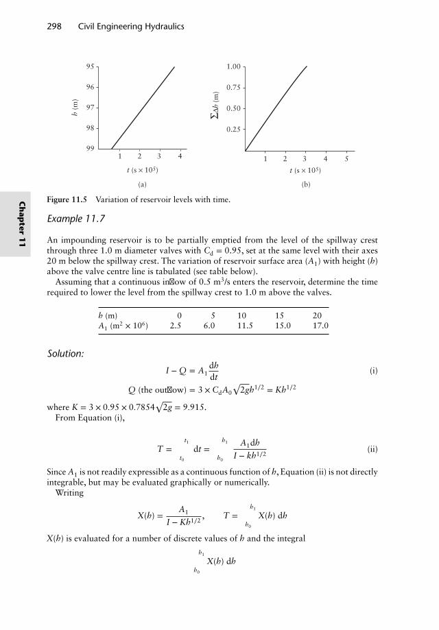
298 Civil Engineering Hydraulics
95
96
97
98
99
1.00
0.75
0.50
0.25
1 2 3 4 1 2 3 4 5
(b)
t (s × 105)t (s × 105)
ΣΔh
(m)
(a)
h (m
)
Figure 11.5 Variation of reservoir levels with time.
Example 11.7
An impounding reservoir is to be partially emptied from the level of the spillway crestthrough three 1.0 m diameter valves with Cd = 0.95, set at the same level with their axes20 m below the spillway crest. The variation of reservoir surface area (A1) with height (h)above the valve centre line is tabulated (see table below).
Assuming that a continuous inflow of 0.5 m3/s enters the reservoir, determine the timerequired to lower the level from the spillway crest to 1.0 m above the valves.
h (m) 0 5 10 15 20A1 (m2 × 106) 2.5 6.0 11.5 15.0 17.0
Solution:
I − Q = A1dhdt
(i)
Q (the outflow) = 3 × CdA0
√2gh1∕2 = Kh1∕2
where K = 3 × 0.95 × 0.7854√
2g = 9.915.From Equation (i),
T = ∫t1
t0
dt = ∫h1
h0
A1dh
I − kh1∕2(ii)
Since A1 is not readily expressible as a continuous function of h, Equation (ii) is not directlyintegrable, but may be evaluated graphically or numerically.
Writing
X(h) =A1
I − Kh1∕2, T = ∫
h1
h0
X(h) dh
X(h) is evaluated for a number of discrete values of h and the integral
∫h1
h0
X(h) dh
Ch
apter
11
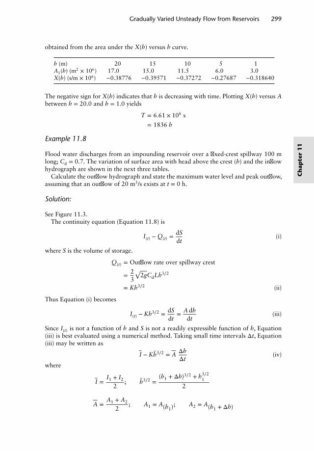
Gradually Varied Unsteady Flow from Reservoirs 299
obtained from the area under the X(h) versus h curve.
h (m) 20 15 10 5 1A1(h) (m2 × 106) 17.0 15.0 11.5 6.0 3.0X(h) (s/m × 106) −0.38776 −0.39571 −0.37272 −0.27687 −0.318640
The negative sign for X(h) indicates that h is decreasing with time. Plotting X(h) versus Abetween h = 20.0 and h = 1.0 yields
T = 6.61 × 10⁶ s
= 1836 h
Example 11.8
Flood water discharges from an impounding reservoir over a fixed-crest spillway 100 mlong; Cd = 0.7. The variation of surface area with head above the crest (h) and the inflowhydrograph are shown in the next three tables.
Calculate the outflow hydrograph and state the maximum water level and peak outflow,assuming that an outflow of 20 m3/s exists at t = 0 h.
Solution:
See Figure 11.3.The continuity equation (Equation 11.8) is
I(t) − Q(t) =dSdt
(i)
where S is the volume of storage.
Q(t) = Outflow rate over spillway crest
= 23
√2gCdLh3∕2
= Kh3∕2 (ii)
Thus Equation (i) becomes
I(t) − Kh3∕2 = dSdt
= A dhdt
(iii)
Since I(t) is not a function of h and S is not a readily expressible function of h, Equation(iii) is best evaluated using a numerical method. Taking small time intervals Δt, Equation(iii) may be written as
I − Kh3∕2 = AΔhΔt
(iv)
where
I =I1 + I2
2; h3∕2 =
(h1 + Δh)3∕2 + h3∕21
2
A =A1 + A2
2; A1 = A(h1); A2 = A(h1 + Δh)
Ch
apte
r1
1
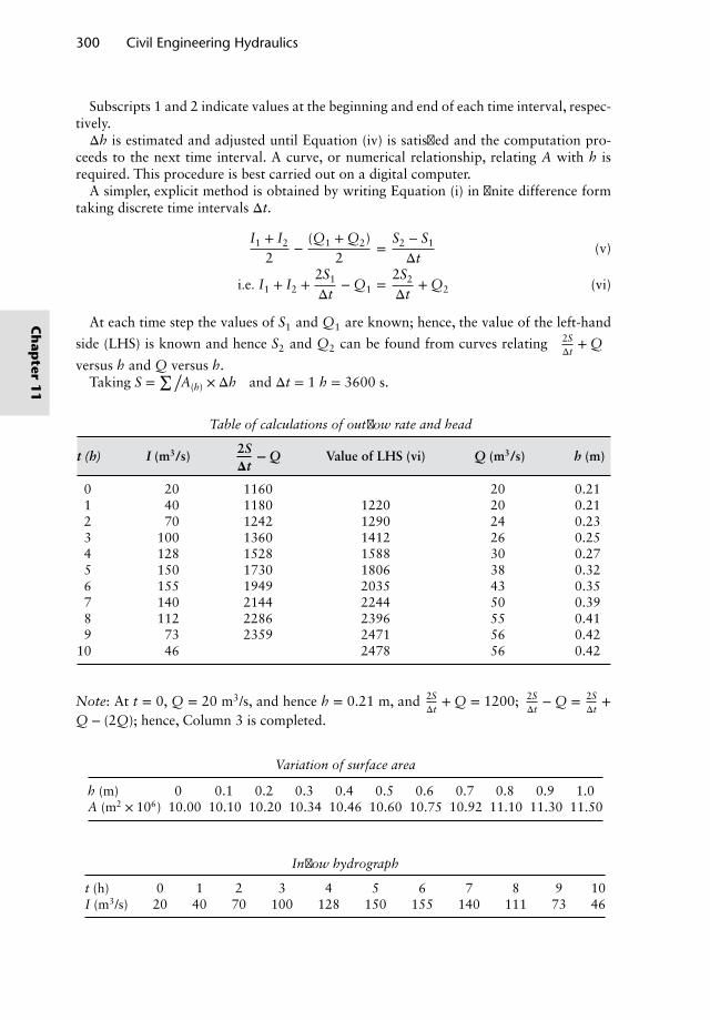
300 Civil Engineering Hydraulics
Subscripts 1 and 2 indicate values at the beginning and end of each time interval, respec-tively.Δh is estimated and adjusted until Equation (iv) is satisfied and the computation pro-
ceeds to the next time interval. A curve, or numerical relationship, relating A with h isrequired. This procedure is best carried out on a digital computer.
A simpler, explicit method is obtained by writing Equation (i) in finite difference formtaking discrete time intervals Δt.
I1 + I2
2−
(Q1 + Q2)2
=S2 − S1
Δt(v)
i.e. I1 + I2 +2S1
Δt− Q1 =
2S2
Δt+ Q2 (vi)
At each time step the values of S1 and Q1 are known; hence, the value of the left-hand
side (LHS) is known and hence S2 and Q2 can be found from curves relating(
2SΔt
+ Q)
versus h and Q versus h.Taking S =
∑(A(h) × Δh
)and Δt = 1 h = 3600 s.
Table of calculations of outflow rate and head
t (h) I (m3/s) 2S𝚫t
− Q Value of LHS (vi) Q (m3/s) h (m)
0 20 1160 20 0.211 40 1180 1220 20 0.212 70 1242 1290 24 0.233 100 1360 1412 26 0.254 128 1528 1588 30 0.275 150 1730 1806 38 0.326 155 1949 2035 43 0.357 140 2144 2244 50 0.398 112 2286 2396 55 0.419 73 2359 2471 56 0.42
10 46 2478 56 0.42
Note: At t = 0, Q = 20 m3/s, and hence h = 0.21 m, and 2SΔt
+ Q = 1200; 2SΔt
− Q = 2SΔt
+Q − (2Q); hence, Column 3 is completed.
Variation of surface area
h (m) 0 0.1 0.2 0.3 0.4 0.5 0.6 0.7 0.8 0.9 1.0A (m2 × 106) 10.00 10.10 10.20 10.34 10.46 10.60 10.75 10.92 11.10 11.30 11.50
Inflow hydrograph
t (h) 0 1 2 3 4 5 6 7 8 9 10I (m3/s) 20 40 70 100 128 150 155 140 111 73 46
Ch
apter
11
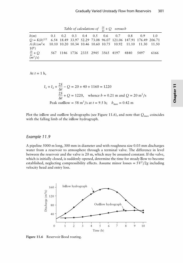
Gradually Varied Unsteady Flow from Reservoirs 301
Table of calculations of(
2SΔt
+ Q)
versus h
h(m) 0.1 0.2 0.3 0.4 0.5 0.6 0.7 0.8 0.9 1.0Q = K(h)3∕2 6.54 18.49 33.97 52.29 73.08 96.07 121.06 147.91 176.49 206.71A (h) (m2× 10.10 10.20 10.34 10.46 10.60 10.75 10.92 11.10 11.30 11.50106)2SΔt
+ Q 567 1146 1736 2335 2945 3565 4197 4840 5497 6166(m3∕s)
At t = 1 h,
I1 + I2 +2SΔt
− Q = 20 + 40 + 1160 = 1220
2SΔt
+ Q = 1220, whence h = 0.21 m and Q = 20 m3∕s
Peak outflow = 58 m3∕s at t = 9.5 h; hmax = 0.42 m
Plot the inflow and outflow hydrographs (see Figure 11.6), and note that Qmax coincideswith the falling limb of the inflow hydrograph.
Example 11.9
A pipeline 5000 m long, 300 mm in diameter and with roughness size 0.03 mm dischargeswater from a reservoir to atmosphere through a terminal valve. The difference in levelbetween the reservoir and the valve is 20 m, which may be assumed constant. If the valve,which is initially closed, is suddenly opened, determine the time for steady flow to becomeestablished, neglecting compressibility effects. Assume minor losses = 5V2∕2g includingvelocity head and entry loss.
Inflow hydrograph
Outflow hydrograph
Time (h)
Dis
char
ge (
m3 /
s)
160
120
80
40
0 1 2 3 4 5 6 7 8 9 10
Figure 11.6 Reservoir flood routing.
Ch
apte
r1
1
302 Civil Engineering Hydraulics
Solution:
From Equation 11.15 and Section 11.3, the theoretical time for flow establishment is
T =LV0
2gHln[
V0 + VV0 − V
]V0
V=0(i)
Using the techniques of Chapter 4 the steady-state velocity V0 under the head of 20 mis calculated to be 1.23 m/s. Theoretically, the time taken to attain steady flow is infinite(substituting V = V0 in Equation (i)); therefore, adopt V0 = 0.99 × 1.23 = 1.2 m/s (say)whence in Equation (i),
T = 5000 × 1.2319.62 × 20
ln[
2.430.03
]= 68.9 s
The above solution assumes a constant value of 𝜆. The reader should evaluate T, takingaccount of the variation of 𝜆 with velocity, using a graphical or numerical integration ofEquation 11.13.
References and recommended reading
Chadwick, A., Morfett, J. and Borthwick, M. (2013) Hydraulics in Civil and EnvironmentalEngineering, 5th edn, Spon, Abingdon, UK.
Mansell, M. G. (2003) Rural and Urban Hydrology, Thomas Telford, London.
Problems
1. A reservoir with a constant plan area of 20 000 m2 discharges water to atmospherethrough a 2000 m long pipeline of 300 mm diameter and roughness 0.15 mm. The reser-voir receives a steady inflow of 20 L/s. If the head between the reservoir surface and thepipe outlet is initially 40 m, determine (neglecting minor losses) the time taken for the headto fall to 35 m.
2. An impounding reservoir of constant area 100 000 m2 discharges to a service reservoirthrough 20 km of 400 mm diameter pipeline of roughness 0.06 mm. Minor losses amountto 20V2∕2g. The impounding reservoir of constant plan area 10 000 m2 receives a steadyinflow of 30 L/s, while a steady outflow of 10 L/s takes place from the service reservoir. Ifthe initial level difference is 50 m, determine the time taken for the head to become 48 mand the time for the level in the upper reservoir to fall by 0.5 m.
3. An impounding reservoir delivers water to a hydroelectric plant through four pipelines,each 2.0 m in diameter and 1000 m in length with a roughness of 0.3 mm. The reservoir isto be drawn down using the four pipelines with bypasses around the turbines to dischargeinto the tailrace which has a constant level. Allowing 5V2∕2g for local losses includingvelocity head, entry and bypass losses, determine the time taken for the level in the reservoirto fall from 50 m above the tailrace to 20 m above the tailrace assuming a constant inflowof 1.0 m3/s. Reservoir surface area data are given in the table below.
Ch
apter
11

Gradually Varied Unsteady Flow from Reservoirs 303
Level above tailrace (m) 20 30 40 50Surface area of reservoir (m2 × 106) 2.0 4.0 6.8 12.2
4. Using the data given for the reservoir in Example 11.8, obtain the outflow hydrographresulting from the following inflow hydrograph if the spillway is 50 m long with Cd = 0.7.Assume the outflow rate at t = 0 to be 10 m3/s.
Time (h) 0 1 2 3 4 5 6 7 8 9 10 11 12Inflow (m3/s) 10 30 80 130 216 250 228 176 120 80 52 44 20
Ch
apte
r1
1

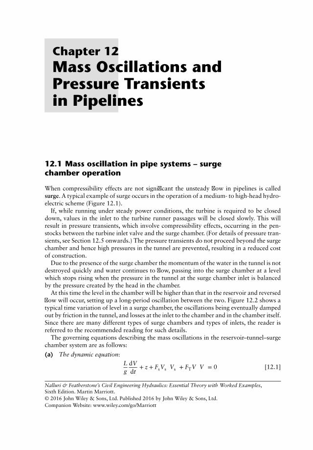
Chapter 12Mass Oscillations andPressure Transientsin Pipelines
12.1 Mass oscillation in pipe systems – surgechamber operation
When compressibility effects are not significant the unsteady flow in pipelines is calledsurge. A typical example of surge occurs in the operation of a medium- to high-head hydro-electric scheme (Figure 12.1).
If, while running under steady power conditions, the turbine is required to be closeddown, values in the inlet to the turbine runner passages will be closed slowly. This willresult in pressure transients, which involve compressibility effects, occurring in the pen-stocks between the turbine inlet valve and the surge chamber. (For details of pressure tran-sients, see Section 12.5 onwards.) The pressure transients do not proceed beyond the surgechamber and hence high pressures in the tunnel are prevented, resulting in a reduced costof construction.
Due to the presence of the surge chamber the momentum of the water in the tunnel is notdestroyed quickly and water continues to flow, passing into the surge chamber at a levelwhich stops rising when the pressure in the tunnel at the surge chamber inlet is balancedby the pressure created by the head in the chamber.
At this time the level in the chamber will be higher than that in the reservoir and reversedflow will occur, setting up a long-period oscillation between the two. Figure 12.2 shows atypical time variation of level in a surge chamber, the oscillations being eventually dampedout by friction in the tunnel, and losses at the inlet to the chamber and in the chamber itself.Since there are many different types of surge chambers and types of inlets, the reader isreferred to the recommended reading for such details.
The governing equations describing the mass oscillations in the reservoir–tunnel–surgechamber system are as follows:
(a) The dynamic equation:Lg
dVdt
+ z + FsVs |Vs| + FTV |V| = 0 [12.1]
Nalluri & Featherstone’s Civil Engineering Hydraulics: Essential Theory with Worked Examples,Sixth Edition. Martin Marriott.© 2016 John Wiley & Sons, Ltd. Published 2016 by John Wiley & Sons, Ltd.Companion Website: www.wiley.com/go/Marriott
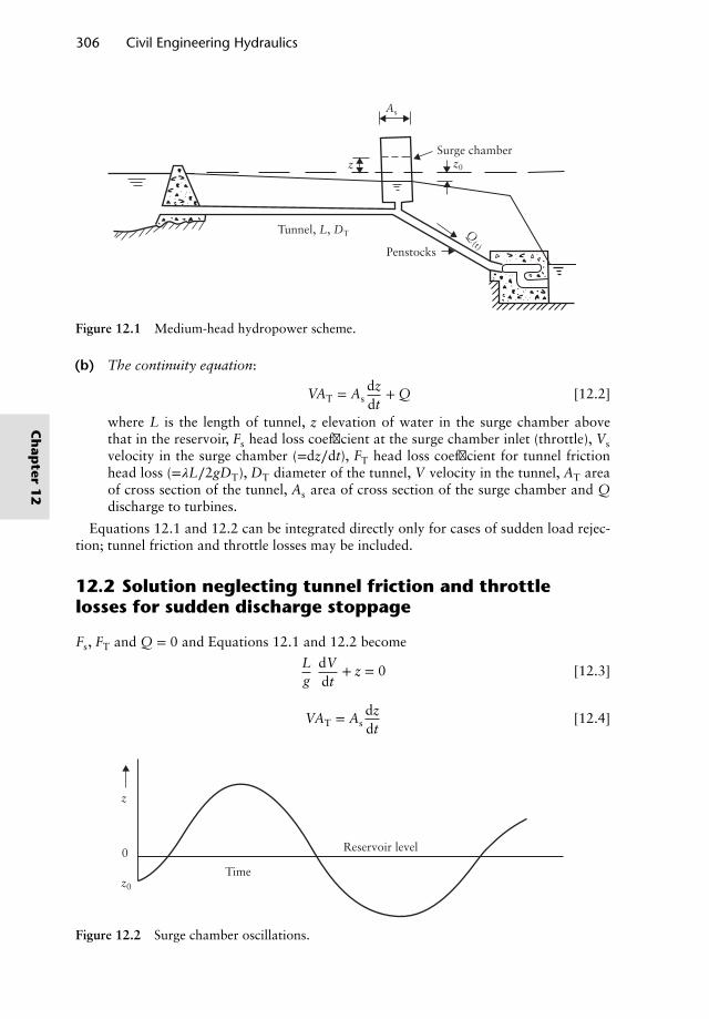
306 Civil Engineering Hydraulics
Tunnel, L, DT
z z0
As
Q(t)
Penstocks
Surge chamber
Figure 12.1 Medium-head hydropower scheme.
(b) The continuity equation:
VAT = Asdzdt
+ Q [12.2]
where L is the length of tunnel, z elevation of water in the surge chamber abovethat in the reservoir, Fs head loss coefficient at the surge chamber inlet (throttle), Vsvelocity in the surge chamber (=dz∕dt), FT head loss coefficient for tunnel frictionhead loss (=𝜆L∕2gDT), DT diameter of the tunnel, V velocity in the tunnel, AT areaof cross section of the tunnel, As area of cross section of the surge chamber and Qdischarge to turbines.
Equations 12.1 and 12.2 can be integrated directly only for cases of sudden load rejec-tion; tunnel friction and throttle losses may be included.
12.2 Solution neglecting tunnel friction and throttlelosses for sudden discharge stoppage
Fs, FT and Q = 0 and Equations 12.1 and 12.2 become
Lg
dVdt
+ z = 0 [12.3]
VAT = Asdzdt
[12.4]
Reservoir level
Time
0
z
z0
Figure 12.2 Surge chamber oscillations.
Ch
apter
12
Mass Oscillations and Pressure Transients in Pipelines 307
Differentiating Equation 12.4,
dVdt
=As
AT
d2zdt2
[12.5]
Hence Lg
As
AT
d2zdt2
+ z = 0 [12.6]
This is a linear, homogeneous, second-order differential equation with constant coefficient,the solution to which is
z = C1 cos2𝜋tT
+ C2 sin2𝜋tT
[12.7]
where T is the period of oscillation. Since the tunnel is assumed to be frictionless, z = 0 att = 0.
Hence z = C2 sin2𝜋tT
[12.8]
T = 2𝜋
√Lg
As
AT[12.9]
dzdt
= C22𝜋T
cos 2𝜋tT
(from Equation 12.8) [12.10]
and dzdt
= VAT
As(from Equation 12.4) [12.11]
Hence V =As
ATC2
2𝜋T
cos 2𝜋tT
when t = 0, V = V0 and V0 =As
ATC2
2𝜋T
[12.12]
Substituting for T from Equation 12.9,
C2 = V0
√Lg
AT
As[12.13]
whence (from Equation 12.8),
z = V0
√Lg
AT
Assin 2𝜋t
T[12.14]
12.3 Solution including tunnel and surge chamber lossesfor sudden discharge stoppage
Since Q = 0, VsAs = VTAT whence Equation 12.1 becomes
Lg
dVdt
+ z +
[Fs
(AT
As
)2
+ FT
]V|V| = 0
or Lg
dVdt
+ z + FRV|V| = 0 [12.15]
Ch
apte
r1
2
308 Civil Engineering Hydraulics
From Equations 12.4, 12.5 and 12.15, the following relationships are obtainable:
V2 = − zFR
+LAT
2gAsF2R
+ C exp(−2gAsFRz
LAT
)[12.16]
when t = 0, V = V0 and z0 = FTV20 whence we obtain
V2 + (z∕FR) − (LAT∕2gAsF2R)
V20 + (FTV2
0∕FR) − (LAT∕2gAsF2R)
= exp
(−2gAsFR(z + FTV2
0 )
LAT
)[12.17]
zmax occurs when V = 0.Note that since dz∕dt = Vs, dt = dz∕Vs, and the time corresponding with any value
of z is
Tz = ∫t
0dt = ∫
z
0
dzVs
= ∫z
0
dzVAT∕As
[12.18]
Equation 12.18 can be evaluated by using a graphical integration or numerical integrationmethod, in the latter case taking small intervals of z.
12.4 Finite difference methods in the solution ofthe surge chamber equations
Numerical methods of analysis using digital computers provide solutions to a wide rangeof operating conditions, and types and shapes of surge chambers.
Considering the general case of a surge chamber with a variable area and taking a finiteinterval Δt during which V changes by ΔV and z changes by Δz, Equations 12.1 and 12.2become
LgΔVΔt
+ zm + FTVm|Vm| + FsVs|Vs| = 0 [12.19]
VmAT = As,mΔzΔt
+ Qm [12.20]
where subscript m indicates the average value in the interval and As,m is the average areaof the surge chamber between z and z + Δz.
(a) Solution by successive estimates. In each time interval, estimate ΔV. Then, Vm =Vi + (ΔV∕2), and from Equation 12.19 calculate zm (=zi + (Δz∕2)) whence z is cal-culated, noting that Vs = Δz∕Δt. Subscript i indicates values at the beginning of thetime interval and which are therefore known. Qm is known since the time variationof discharge to the turbines will be prescribed and substitution of Δz into Equation12.20 yields Vm. If the two values of Vm agree, the estimated value of ΔV is correct;otherwise adjust ΔV and repeat until agreement is achieved and proceed to the nexttime interval.
Alternatively, estimate Δz and proceed in similar fashion; this is preferable if thechamber has a variable area. In both cases the time variation of z is obtained.
Such calculations are ideally carried out on a computer spreadsheet.
Ch
apter
12
Mass Oscillations and Pressure Transients in Pipelines 309
(b) Direct solution of Equations 12.19 and 12.20. From Equation 12.20,
Δz = ΔtAs,m
(ViAT +
AT
2ΔV − Qm
)[12.21]
where Vm = Vi +ΔV2
Also zm = zi + (Δz∕2) and Vs = Δz∕Δt; Equation 12.19 becomes
Lg
ΔVΔt
+ zi +Δt2As
(ViAT +
AT
2ΔV − Qm
)± FT
(Vi +
ΔV2
)2
±Fs
A2s
[A2
T
(V2
i + Vi ΔV + ΔV2
4
)− 2AT
(Vi +
ΔV2
)Qm + Q2
m
]= 0
Rearranging
±FR
4ΔV2 +
[L
gΔt+
AT
4As,mΔt ±
(FRVi −
FsATQm
A2s
)]ΔV + zi
+AT
2As,mVi Δt −
Qm
2As,mΔt ±
[FRV2
i +Fs
A2s
Qm
(− 2ViAT + Qm
)]= 0 [12.22]
which is of the form
aΔV2 + bΔV + c = 0 [12.23]
whence ΔV = −b +√
b2 − 4ac2a
[12.24]
ΔV is therefore determined explicitly in each successive time step Δt, and the cor-responding change in z is obtained from Equation 12.21. Note that if V becomesnegative (i.e. on the downswing) the negative value of FR is used. As with most finitedifference methods, in this case Δt should be small since the use of average valuesof the variables implies a linear time variation. A 10 s time interval usually gives asufficiently accurate solution.
12.5 Pressure transients in pipelines (waterhammer)
Changes in the discharge in pipelines, caused by valve or pump operation, either closureor opening, result in pressure surges which are propagated along the pipeline from thesource. If the changes in control are gradual, the time variation of pressures and dischargemay be achieved by assuming the liquid to be incompressible and neglecting the elasticproperties of the pipeline such as in the problems on surge analysis dealt with in Sections12.1–12.4.
In the case of rapid valve closure or pump stoppage, the resulting deceleration of theliquid column causes pressure surges having large pressure differences across the wavefront. The speed (celerity) of the pressure wave is dependent on the compressibility of theliquid and the elasticity of the pipeline, and these parameters are therefore incorporatedin the analysis.
Ch
apte
r1
2
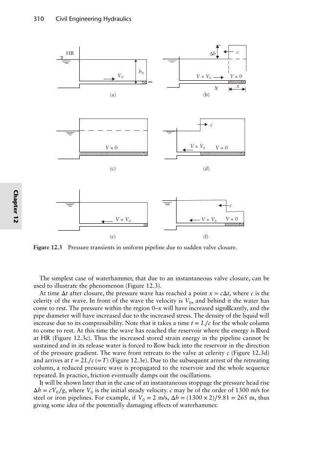
310 Civil Engineering Hydraulics
h0V0
HR
(b)(a)
(d)(c)
(f)(e)
V = V0
V = V0
V = V0 V = V0
Δh
X x
c
c
c
V = 0
V = 0
V = 0
V = 0
Figure 12.3 Pressure transients in uniform pipeline due to sudden valve closure.
The simplest case of waterhammer, that due to an instantaneous valve closure, can beused to illustrate the phenomenon (Figure 12.3).
At time Δt after closure, the pressure wave has reached a point x = cΔt, where c is thecelerity of the wave. In front of the wave the velocity is V0, and behind it the water hascome to rest. The pressure within the region 0–x will have increased significantly, and thepipe diameter will have increased due to the increased stress. The density of the liquid willincrease due to its compressibility. Note that it takes a time t = L∕c for the whole columnto come to rest. At this time the wave has reached the reservoir where the energy is fixedat HR (Figure 12.3c). Thus the increased stored strain energy in the pipeline cannot besustained and in its release water is forced to flow back into the reservoir in the directionof the pressure gradient. The wave front retreats to the valve at celerity c (Figure 12.3d)and arrives at t = 2L∕c (=T) (Figure 12.3e). Due to the subsequent arrest of the retreatingcolumn, a reduced pressure wave is propagated to the reservoir and the whole sequencerepeated. In practice, friction eventually damps out the oscillations.
It will be shown later that in the case of an instantaneous stoppage the pressure head riseΔh = cV0∕g, where V0 is the initial steady velocity. c may be of the order of 1300 m/s forsteel or iron pipelines. For example, if V0 = 2 m/s, Δh = (1300 × 2)∕9.81 = 265 m, thusgiving some idea of the potentially damaging effects of waterhammer.
Ch
apter
12
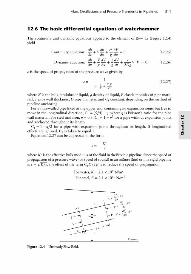
Mass Oscillations and Pressure Transients in Pipelines 311
12.6 The basic differential equations of waterhammer
The continuity and dynamic equations applied to the element of flow 𝛿x (Figure 12.4)yield
Continuity equation: 𝜕h𝜕t
+ V𝜕h𝜕x
+ c2
g𝜕V𝜕x
= 0 [12.25]
Dynamic equation: 𝜕h𝜕x
+ Vg𝜕V𝜕x
+ 1g𝜕V𝜕t
+ 𝜆
2DgV |V| = 0 [12.26]
c is the speed of propagation of the pressure wave given by
c =√√√√ 1
𝜌
(1K+ C1D
TE
) [12.27]
where K is the bulk modulus of liquid, 𝜌 density of liquid, E elastic modules of pipe mate-rial, T pipe wall thickness,D pipe diameter, and C1 constant, depending on the method ofpipeline anchoring.
For a thin-walled pipe fixed at the upper end, containing no expansion joints but free tomove in the longitudinal direction, C1 = (5∕4) − 𝜂, where 𝜂 is Poisson’s ratio for the pipewall material. For steel and iron, 𝜂 = 0.3. C1 = 1 − 𝜂2 for a pipe without expansion jointsand anchored throughout its length.
C1 = 1 − 𝜂∕2 for a pipe with expansion joints throughout its length. If longitudinaleffects are ignored, C1 is taken to equal 1.
Equation 12.27 can be expressed in the form
c =√
K∗
𝜌
where K∗ is the effective bulk modulus of the fluid in the flexible pipeline. Since the speed ofpropagation of a pressure wave (or speed of sound) in an infinite fluid or in a rigid pipelineis c =
√K∕𝜌, the effect of the term C1D∕TE is to reduce the speed of propagation.
For water, K = 2.1 × 10⁹ N/m2
For steel, E = 2.1 × 10¹¹ N/m2
P
A
h
V
xz
A +δx∂A
∂x
p +δx∂p
∂x
V +δx
δx
∂V∂x
Datum
Figure 12.4 Unsteady flow field.
Ch
apte
r1
2
312 Civil Engineering Hydraulics
12.7 Solutions of the waterhammer equations
Equations 12.25 and 12.26 can be solved analytically only if certain simplifying assump-tions are made, such as the neglect of certain terms, and for simple boundary conditionssuch as reservoirs and valves. Some methods neglect friction losses, which can lead toserious errors in the calculation of pressure transients.
Since the advent of the digital computer, Equations 12.25 and 12.26 when expressed indiscretised form can be readily evaluated for a whole range of boundary conditions andpipe configurations including networks. The computations proceed in small time steps, andthe pipeline is ‘divided’ into equal sections. At every ‘station’ between adjacent sections,the transient pressure head and velocity are calculated at each time step. In this way thecomplete history of the waterhammer in space and time is revealed. No simplifyingassumptions to the basic equations need be made. Indeed, if interior boundary conditionssuch as low pressures causing cavitation arise, especially in sloping pipelines, these can beincorporated in the analysis.
The most commonly used numerical method is probably the method of ‘characteris-tics’ which reduces the partial differential equations to a pair of simultaneous ordinarydifferential equations. These when expressed in numerical (finite difference) form can beprogrammed for automatic evaluation on a digital computer. Such methods are, however,beyond the scope of this text.
In the present day, therefore, it hardly seems justifiable to use simplified methods. How-ever, in the following sections some of these methods will be illustrated. These were devel-oped before the advent of computers and represent examples of classic analytical tech-niques. In some cases friction can be included, and the results, for example for the pressuretransients at closing valves, are very similar to those obtained using the ‘characteristics’method. Friction losses are often simplified by assuming them to be localised, for exampleat an ‘orifice’ at the outlet from a reservoir. Such losses may also be discretely distributedalong the pipeline but this makes the analysis more laborious.
The analytical methods which are included hereafter illustrate some aspects of the water-hammer phenomenon. The inclusion of additional features has been kept to a minimumin view of the superiority of numerical analysis for practical problems.
12.8 The Allievi equations
The differential Equations 12.25 and 12.26 cannot be solved analytically unless certainsimplifications are carried out.
The term V𝜕h∕𝜕x is of the order of [V∕(V + c)]∕(𝜕h∕𝜕t) and may therefore be small.𝜕V∕𝜕x is small compared with 𝜕V∕𝜕t since
dVdt
= −V 𝜕V𝜕x
+ 𝜕V𝜕t
= 𝜕V𝜕t
(1 − V 𝜕V
𝜕x𝜕t𝜕V
)= 𝜕V
𝜕t
(1 − V
𝜕x∕𝜕t
)
in which the last term is small.
Ch
apter
12
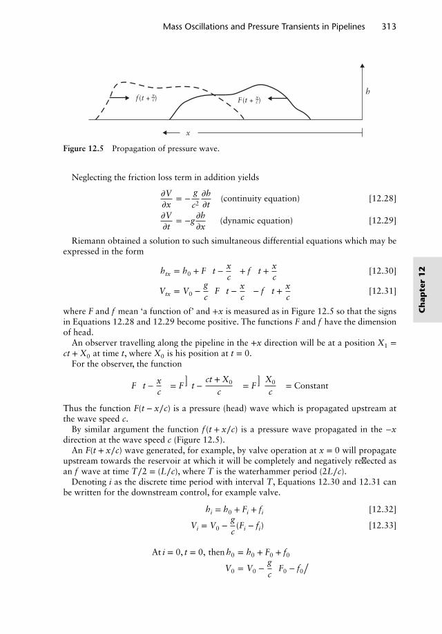
Mass Oscillations and Pressure Transients in Pipelines 313
h
x
F (t + xc)f (t + xc)
Figure 12.5 Propagation of pressure wave.
Neglecting the friction loss term in addition yields
𝜕V𝜕x
= −g
c2
𝜕h𝜕t
(continuity equation) [12.28]
𝜕V𝜕t
= −g𝜕h𝜕x
(dynamic equation) [12.29]
Riemann obtained a solution to such simultaneous differential equations which may beexpressed in the form
htx = h0 + F(
t − xc
)+ f
(t + x
c
)[12.30]
Vtx = V0 −gc
[F(
t − xc
)− f
(t + x
c
)][12.31]
where F and f mean ‘a function of’ and +x is measured as in Figure 12.5 so that the signsin Equations 12.28 and 12.29 become positive. The functions F and f have the dimensionof head.
An observer travelling along the pipeline in the +x direction will be at a position X1 =ct +X0 at time t, where X0 is his position at t = 0.
For the observer, the function
F(
t − xc
)= F
(t −
ct +X0
c
)= F
(X0
c
)= Constant
Thus the function F(t − x∕c) is a pressure (head) wave which is propagated upstream atthe wave speed c.
By similar argument the function f (t + x∕c) is a pressure wave propagated in the −xdirection at the wave speed c (Figure 12.5).
An F(t + x∕c) wave generated, for example, by valve operation at x = 0 will propagateupstream towards the reservoir at which it will be completely and negatively reflected asan f wave at time T∕2 = (L∕c), where T is the waterhammer period (2L∕c).
Denoting i as the discrete time period with interval T, Equations 12.30 and 12.31 canbe written for the downstream control, for example valve.
hi = h0 + Fi + fi [12.32]
Vi = V0 −gc
(Fi − fi) [12.33]
At i = 0, t = 0, then h0 = h0 + F0 + f0
V0 = V0 −gc
(F0 − f0
)
Ch
apte
r1
2
314 Civil Engineering Hydraulics
At i = 1, t = T, then h1 = h0 + F1 + f1
V1 = V0 −gc
(F1 − f1
)and so on.
Since f is the reflected F wave, f0 = 0, f1 = −F0, f2 = −F1 and so on. Thus,
h1 = h0 + F1 − F0
V1 = V0 −gc
(F1 + F0)
and
h2 = h0 + F2 − F1
V2 = V0 −gc
(F2 + F1)
Adding successive pairs of head equations and subtracting successive pairs of velocityequations,
h1 + h0 = 2h0 + F1
h2 + h1 = 2h0 + F2 − F0
V0 − V1 =gc
(F1 + F0)
V1 − V2 = −gc
(F0 − F2)
whence, in general,
Fi − Fi−2 = cg
(Vi−1 − Vi)
hi + hi−1 − 2h0 = cg
(Vi−1 − Vi) [12.34]
Boundary conditions may be set at the valve at the downstream end.The discharge through a valve of area Av,i at time i when the pressure head behind it is
hi is given by
Q = Cd,iAv,i
√2ghi [12.35]
and the velocity in the pipe immediately upstream is
Vi =Cd,iAv,i
Ap
√2ghi [12.36]
where Ap is the area of the pipe and Cd,i the discharge coefficient.The ratio
Vi
V0=
Cd,iAv,i
Cd,0Av,0
√hi√h0
Denoting
𝜂i =Cd,iAv,i
Cd,0Av,0and 𝜉2
i =hi
h0
Vi = V0𝜂i𝜉i [12.37]
and hi = h0𝜉2i [12.38]
Ch
apter
12
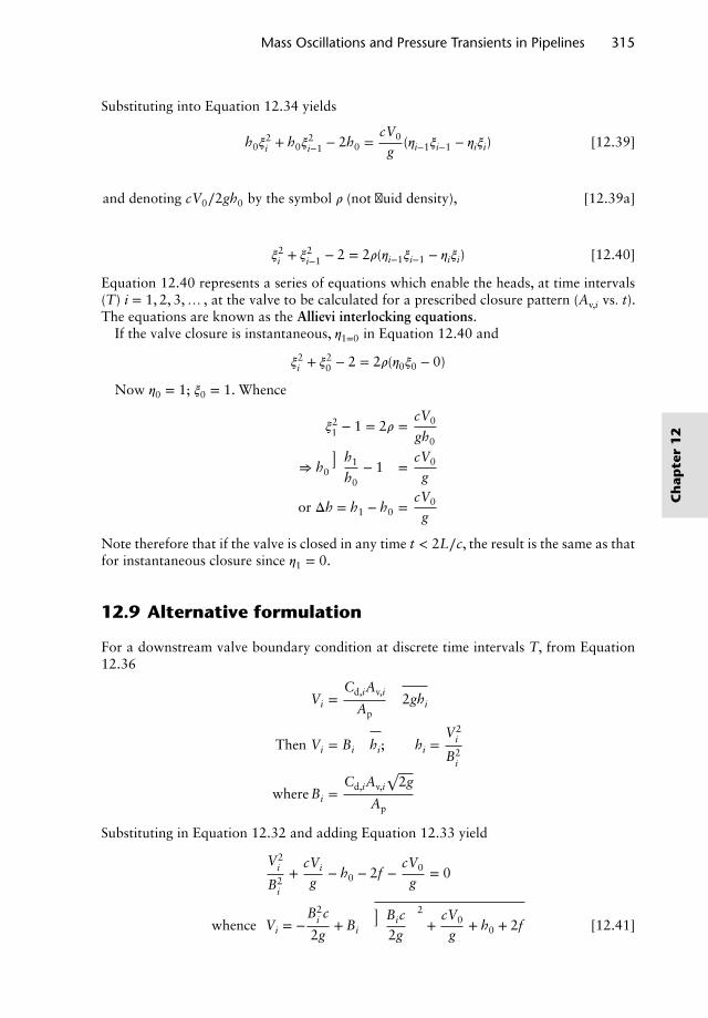
Mass Oscillations and Pressure Transients in Pipelines 315
Substituting into Equation 12.34 yields
h0𝜉2i + h0𝜉
2i−1 − 2h0 =
cV0
g(𝜂i−1𝜉i−1 − 𝜂i𝜉i) [12.39]
and denoting cV0∕2gh0 by the symbol 𝜌 (not fluid density), [12.39a]
𝜉2i + 𝜉2
i−1 − 2 = 2𝜌(𝜂i−1𝜉i−1 − 𝜂i𝜉i) [12.40]
Equation 12.40 represents a series of equations which enable the heads, at time intervals(T) i = 1, 2, 3,… , at the valve to be calculated for a prescribed closure pattern (Av,i vs. t).The equations are known as the Allievi interlocking equations.
If the valve closure is instantaneous, 𝜂1=0 in Equation 12.40 and
𝜉2i + 𝜉2
0 − 2 = 2𝜌(𝜂0𝜉0 − 0)
Now 𝜂0 = 1; 𝜉0 = 1. Whence
𝜉21 − 1 = 2𝜌 =
cV0
gh0
⇒ h0
(h1
h0− 1
)=
cV0
g
or Δh = h1 − h0 =cV0
g
Note therefore that if the valve is closed in any time t < 2L∕c, the result is the same as thatfor instantaneous closure since 𝜂1 = 0.
12.9 Alternative formulation
For a downstream valve boundary condition at discrete time intervals T, from Equation12.36
Vi =Cd,iAv,i
Ap
√2ghi
Then Vi = Bi
√hi; hi =
V2i
B2i
where Bi =Cd,iAv,i
√2g
Ap
Substituting in Equation 12.32 and adding Equation 12.33 yield
V2i
B2i
+cVi
g− h0 − 2f −
cV0
g= 0
whence Vi = −B2
i c
2g+ Bi
√(Bic2g
)2
+cV0
g+ h0 + 2f [12.41]
Ch
apte
r1
2
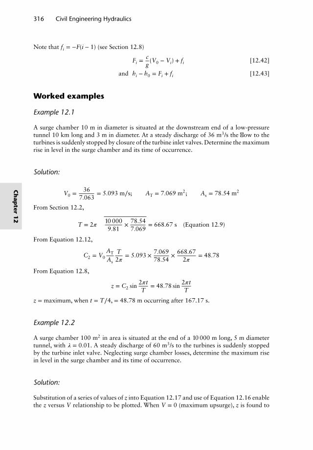
316 Civil Engineering Hydraulics
Note that fi = −F(i − 1) (see Section 12.8)
Fi =cg
(V0 − Vi) + fi [12.42]
and hi − h0 = Fi + fi [12.43]
Worked examples
Example 12.1
A surge chamber 10 m in diameter is situated at the downstream end of a low-pressuretunnel 10 km long and 3 m in diameter. At a steady discharge of 36 m3/s the flow to theturbines is suddenly stopped by closure of the turbine inlet valves. Determine the maximumrise in level in the surge chamber and its time of occurrence.
Solution:
V0 = 367.063
= 5.093 m∕s; AT = 7.069 m2; As = 78.54 m2
From Section 12.2,
T = 2𝜋
√10 0009.81
× 78.547.069
= 668.67 s (Equation 12.9)
From Equation 12.12,
C2 = V0AT
As
T2𝜋
= 5.093 × 7.06978.54
× 668.672𝜋
= 48.78
From Equation 12.8,
z = C2 sin2𝜋tT
= 48.78 sin 2𝜋tT
z = maximum, when t = T∕4, = 48.78 m occurring after 167.17 s.
Example 12.2
A surge chamber 100 m2 in area is situated at the end of a 10 000 m long, 5 m diametertunnel, with 𝜆 = 0.01. A steady discharge of 60 m3/s to the turbines is suddenly stoppedby the turbine inlet valve. Neglecting surge chamber losses, determine the maximum risein level in the surge chamber and its time of occurrence.
Solution:
Substitution of a series of values of z into Equation 12.17 and use of Equation 12.16 enablethe z versus V relationship to be plotted. When V = 0 (maximum upsurge), z is found to
Ch
apter
12
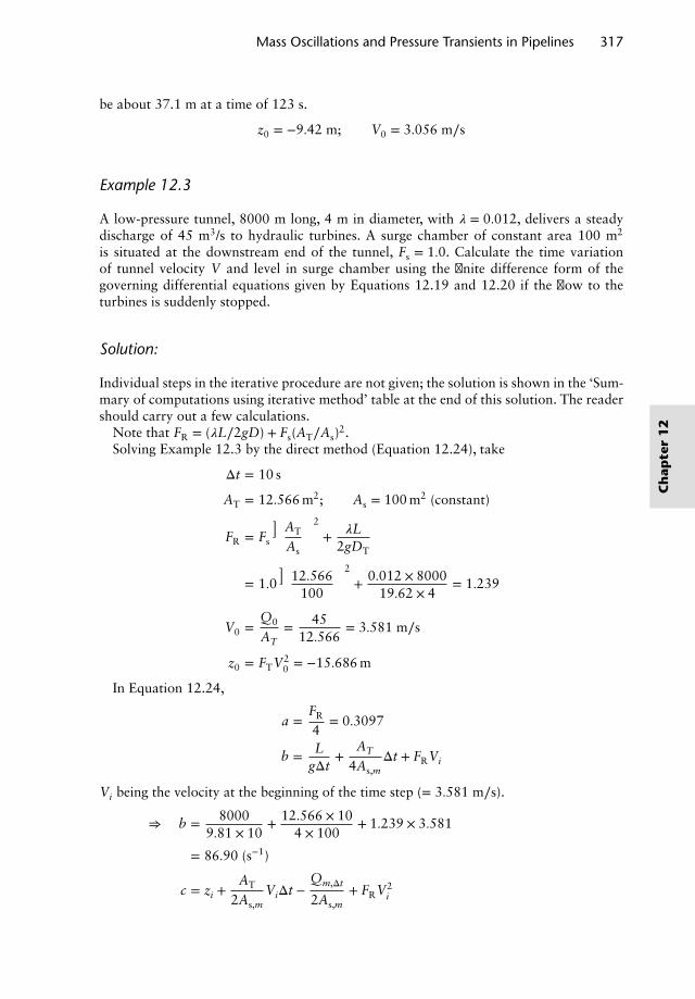
Mass Oscillations and Pressure Transients in Pipelines 317
be about 37.1 m at a time of 123 s.
z0 = −9.42 m; V0 = 3.056 m∕s
Example 12.3
A low-pressure tunnel, 8000 m long, 4 m in diameter, with 𝜆 = 0.012, delivers a steadydischarge of 45 m3/s to hydraulic turbines. A surge chamber of constant area 100 m2
is situated at the downstream end of the tunnel, Fs = 1.0. Calculate the time variationof tunnel velocity V and level in surge chamber using the finite difference form of thegoverning differential equations given by Equations 12.19 and 12.20 if the flow to theturbines is suddenly stopped.
Solution:
Individual steps in the iterative procedure are not given; the solution is shown in the ‘Sum-mary of computations using iterative method’ table at the end of this solution. The readershould carry out a few calculations.
Note that FR = (𝜆L∕2gD) + Fs(AT∕As)2.
Solving Example 12.3 by the direct method (Equation 12.24), take
Δt = 10 s
AT = 12.566 m2; As = 100 m2 (constant)
FR = Fs
(AT
As
)2
+ 𝜆L2gDT
= 1.0(
12.566100
)2
+ 0.012 × 800019.62 × 4
= 1.239
V0 =Q0
AT= 45
12.566= 3.581 m∕s
z0 = FTV20 = −15.686 m
In Equation 12.24,
a =FR
4= 0.3097
b = LgΔt
+AT
4As,mΔt + FRVi
Vi being the velocity at the beginning of the time step (= 3.581 m∕s).
⇒ b = 80009.81 × 10
+ 12.566 × 104 × 100
+ 1.239 × 3.581
= 86.90 (s−1)
c = zi +AT
2As,mViΔt −
Qm,Δt
2As,m+ FRV2
i
Ch
apte
r1
2
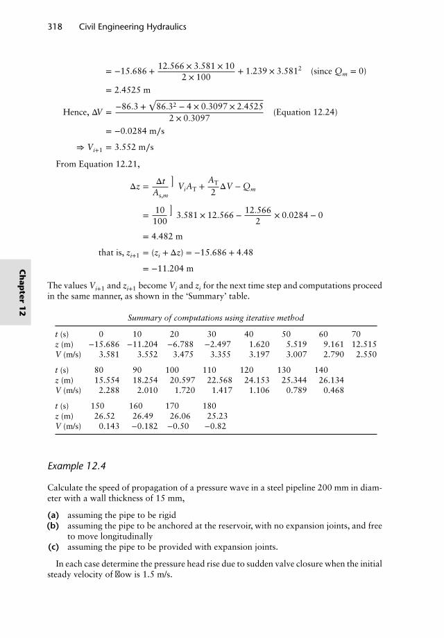
318 Civil Engineering Hydraulics
= −15.686 + 12.566 × 3.581 × 102 × 100
+ 1.239 × 3.5812 (since Qm = 0)
= 2.4525 m
Hence, ΔV = −86.3 +√
86.32 − 4 × 0.3097 × 2.45252 × 0.3097
(Equation 12.24)
= −0.0284 m∕s
⇒ Vi+1 = 3.552 m∕s
From Equation 12.21,
Δz = ΔtAs,m
(ViAT +
AT
2ΔV − Qm
)
= 10100
(3.581 × 12.566 − 12.566
2× 0.0284 − 0
)= 4.482 m
that is, zi+1 = (zi + Δz) = −15.686 + 4.48
= −11.204 m
The values Vi+1 and zi+1 become Vi and zi for the next time step and computations proceedin the same manner, as shown in the ‘Summary’ table.
Summary of computations using iterative method
t (s) 0 10 20 30 40 50 60 70z (m) −15.686 −11.204 −6.788 −2.497 1.620 5.519 9.161 12.515V (m/s) 3.581 3.552 3.475 3.355 3.197 3.007 2.790 2.550
t (s) 80 90 100 110 120 130 140z (m) 15.554 18.254 20.597 22.568 24.153 25.344 26.134V (m/s) 2.288 2.010 1.720 1.417 1.106 0.789 0.468
t (s) 150 160 170 180z (m) 26.52 26.49 26.06 25.23V (m/s) 0.143 −0.182 −0.50 −0.82
Example 12.4
Calculate the speed of propagation of a pressure wave in a steel pipeline 200 mm in diam-eter with a wall thickness of 15 mm,
(a) assuming the pipe to be rigid(b) assuming the pipe to be anchored at the reservoir, with no expansion joints, and free
to move longitudinally(c) assuming the pipe to be provided with expansion joints.
In each case determine the pressure head rise due to sudden valve closure when the initialsteady velocity of flow is 1.5 m/s.
Ch
apter
12
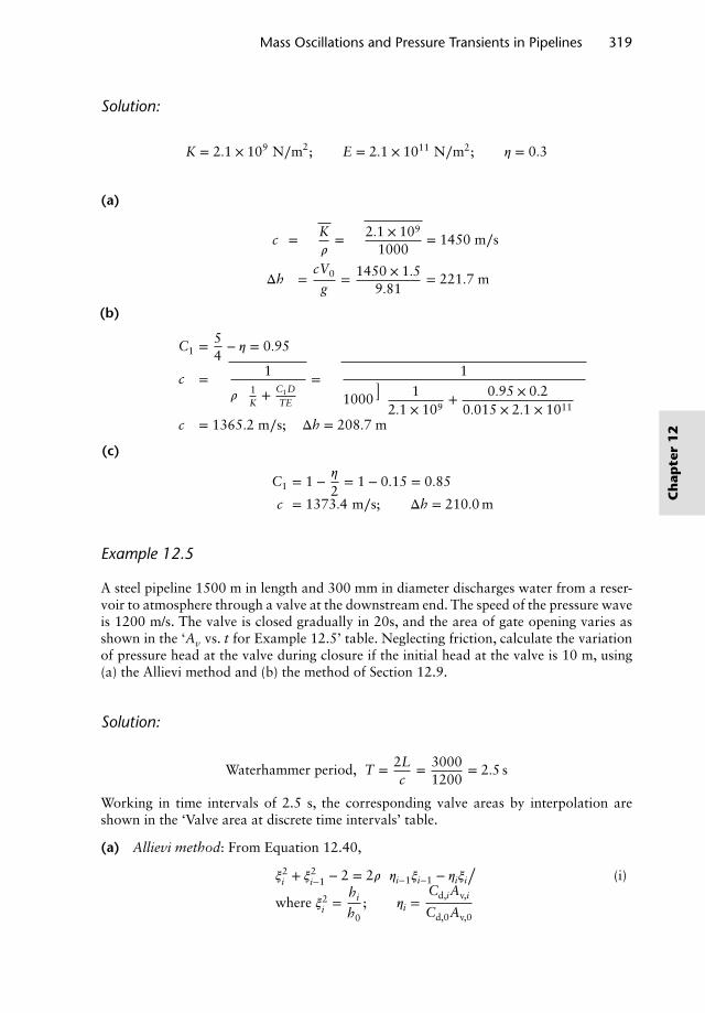
Mass Oscillations and Pressure Transients in Pipelines 319
Solution:
K = 2.1 × 10⁹ N∕m2; E = 2.1 × 10¹¹ N∕m2; 𝜂 = 0.3
(a)
c =√
K𝜌
=√
2.1 × 10⁹
1000= 1450 m∕s
Δh =cV0
g= 1450 × 1.5
9.81= 221.7 m
(b)
C1 = 54− 𝜂 = 0.95
c =√√√√ 1
𝜌
(1K+ C1D
TE
) =√√√√√ 1
1000(
12.1 × 10⁹
+ 0.95 × 0.20.015 × 2.1 × 1011
)c = 1365.2 m∕s; Δh = 208.7 m
(c)
C1 = 1 − 𝜂
2= 1 − 0.15 = 0.85
c = 1373.4 m∕s; Δh = 210.0 m
Example 12.5
A steel pipeline 1500 m in length and 300 mm in diameter discharges water from a reser-voir to atmosphere through a valve at the downstream end. The speed of the pressure waveis 1200 m/s. The valve is closed gradually in 20s, and the area of gate opening varies asshown in the ‘Av vs. t for Example 12.5’ table. Neglecting friction, calculate the variationof pressure head at the valve during closure if the initial head at the valve is 10 m, using(a) the Allievi method and (b) the method of Section 12.9.
Solution:
Waterhammer period, T = 2Lc
= 30001200
= 2.5 s
Working in time intervals of 2.5 s, the corresponding valve areas by interpolation areshown in the ‘Valve area at discrete time intervals’ table.
(a) Allievi method: From Equation 12.40,
𝜉2i + 𝜉2
i−1 − 2 = 2𝜌(𝜂i−1𝜉i−1 − 𝜂i𝜉i
)(i)
where 𝜉2i =
hi
h0; 𝜂i =
Cd,iAv,i
Cd,0Av,0
Ch
apte
r1
2
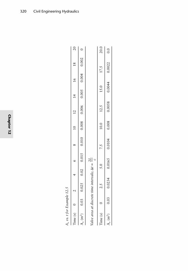
320 Civil Engineering Hydraulics
Av
vs.t
for
Exa
mpl
e12
.5
Tim
e(s
)0
24
68
1012
1416
1820
Av
(m2)
0.03
0.02
50.
020.
015
0.01
00.
008
0.00
60.
005
0.00
40.
002
0
Val
vear
eaat
disc
rete
tim
ein
terv
als;Δ
t=
2L c
Tim
e(s
)0
2.5
5.0
7.5
10.0
12.5
15.0
17.5
20.0
Av
(m2)
0.03
0.02
340.
0165
0.01
040.
008
0.00
580.
0044
0.00
220.
0
Ch
apter
12
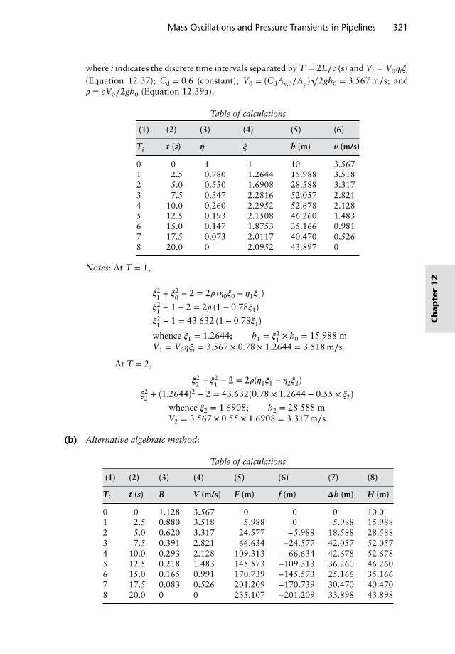
Mass Oscillations and Pressure Transients in Pipelines 321
where i indicates the discrete time intervals separated by T = 2L∕c (s) and Vi = V0𝜂i𝜉i
(Equation 12.37); Cd = 0.6 (constant); V0 = (CdAv,0∕Ap)√
2gh0 = 3.567 m∕s; and𝜌 = cV0∕2gh0 (Equation 12.39a).
Table of calculations
(1) (2) (3) (4) (5) (6)
Ti t (s) 𝜼 𝝃 h (m) v (m/s)
0 0 1 1 10 3.5671 2.5 0.780 1.2644 15.988 3.5182 5.0 0.550 1.6908 28.588 3.3173 7.5 0.347 2.2816 52.057 2.8214 10.0 0.260 2.2952 52.678 2.1285 12.5 0.193 2.1508 46.260 1.4836 15.0 0.147 1.8753 35.166 0.9817 17.5 0.073 2.0117 40.470 0.5268 20.0 0 2.0952 43.897 0
Notes: At T = 1,
𝜉21 + 𝜉2
0 − 2 = 2𝜌 (𝜂0𝜉0 − 𝜂1𝜉1)
𝜉21 + 1 − 2 = 2𝜌 (1 − 0.78𝜉1)
𝜉21 − 1 = 43.632 (1 − 0.78𝜉1)
whence 𝜉1 = 1.2644; h1 = 𝜉21 × h0 = 15.988 m
V1 = V0𝜂𝜉i = 3.567 × 0.78 × 1.2644 = 3.518 m∕s
At T = 2,
𝜉22 + 𝜉2
1 − 2 = 2𝜌(𝜂1𝜉1 − 𝜂2𝜉2)
𝜉22 + (1.2644)2 − 2 = 43.632(0.78 × 1.2644 − 0.55 × 𝜉2)
whence 𝜉2 = 1.6908; h2 = 28.588 mV2 = 3.567 × 0.55 × 1.6908 = 3.317 m∕s
(b) Alternative algebraic method:
Table of calculations
(1) (2) (3) (4) (5) (6) (7) (8)
Ti t (s) B V (m/s) F (m) f (m) 𝚫h (m) H (m)
0 0 1.128 3.567 0 0 0 10.01 2.5 0.880 3.518 5.988 0 5.988 15.9882 5.0 0.620 3.317 24.577 −5.988 18.588 28.5883 7.5 0.391 2.821 66.634 −24.577 42.057 52.0574 10.0 0.293 2.128 109.313 −66.634 42.678 52.6785 12.5 0.218 1.483 145.573 −109.313 36.260 46.2606 15.0 0.165 0.991 170.739 −145.573 25.166 35.1667 17.5 0.083 0.526 201.209 −170.739 30.470 40.4708 20.0 0 0 235.107 −201.209 33.898 43.898
Ch
apte
r1
2
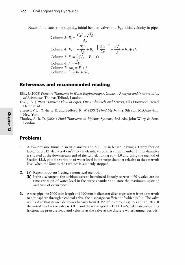
322 Civil Engineering Hydraulics
Notes: i indicates time step; h0, initial head at valve; and V0, initial velocity in pipe.
Column 3: Bi =CdAvi
√2g
Ap
Column 4: Vi = −B2
i c
2g+ Bi
√(Bic2g
)2
+cV0
g+ h0 + 2fi
Column 5: Fi =cg
(V0 − Vi + f )
Column 6: fi = −Fi−1Column 7: Δhi = Fi + fiColumn 8: hi = h0 + Δhi
References and recommended reading
Ellis, J. (2008) Pressure Transients in Water Engineering: A Guide to Analysis and Interpretationof Behaviour, Thomas Telford, London.
Fox, J. A. (1989) Transient Flow in Pipes, Open Channels and Sewers, Ellis Horwood, HemelHempstead.
Streeter, V. L., Wylie, E. B. and Bedford, K. W. (1997) Fluid Mechanics, 9th edn, McGraw-Hill,New York.
Thorley, A. R. D. (2004) Fluid Transients in Pipeline Systems, 2nd edn, John Wiley & Sons,London.
Problems
1. A low-pressure tunnel 4 m in diameter and 8000 m in length, having a Darcy frictionfactor of 0.012, delivers 45 m3/s to a hydraulic turbine. A surge chamber 8 m in diameteris situated at the downstream end of the tunnel. Taking Fs = 1.0 and using the method ofSection 12.3, plot the variation of water level in the surge chamber relative to the reservoirlevel when the flow to the turbines is suddenly stopped.
2. (a) Repeat Problem 1 using a numerical method.(b) If the discharge to the turbines were to be reduced linearly to zero in 90 s, calculate the
time variation of water level in the surge chamber and state the maximum upswingand time of occurrence.
3. A steel pipeline 2000 m in length and 300 mm in diameter discharges water from a reservoirto atmosphere through a control valve, the discharge coefficient of which is 0.6. The valveis closed so that its area decreases linearly from 0.065 m2 to zero in (a) 15 s and (b) 30 s. Ifthe initial head at the valve is 3.0 m and the wave speed is 1333.3 m/s, calculate, neglectingfriction, the pressure head and velocity at the valve at the discrete waterhammer periods.
Ch
apter
12
Chapter 13Unsteady Flow in Channels
13.1 Introduction
River flood propagation, estuarial flows and surges resulting from gate operation or damfailure are practical examples of unsteady channel flows. Natural flood flows in riversand the propagation of tides in estuaries are examples of gradually varied unsteady flowsince the vertical component of acceleration is small. Surges are examples of rapidly variedunsteady flow.
Consider the two-dimensional propagation of a low wave which has a small height inrelation to its wavelength (see Figure 13.1). The celerity or speed of propagation relativeto the water is given by
√gy, where y is the water depth. Therefore the velocity of the
wave relative to a stationary observer is
c =√
gy ± V [13.1]
Note that the Froude number Fr expressed by V∕√
gy is the ratio of water velocity to wavecelerity. If the Froude number is greater than unity, which corresponds with supercriticalflow, a small gravity wave cannot be propagated upstream. Waves of finite height are dealtwith in Sections 13.3 and following sections.
13.2 Gradually varied unsteady flow
Examples of gradually varied unsteady flow are floodwaves and estuarial flows; in suchwaves the rate of change of depth is gradual.
In one-dimensional form (i.e. depth and width integrated) it can be shown that the twogoverning continuity and dynamic partial differential equations are
𝜕Q𝜕x
+ 𝜕A𝜕t
= 0 [13.2]
𝜕y𝜕x
+ Vg𝜕V𝜕x
+ 1g𝜕V𝜕t
= S0 − Sf [13.3]
Nalluri & Featherstone’s Civil Engineering Hydraulics: Essential Theory with Worked Examples,Sixth Edition. Martin Marriott.© 2016 John Wiley & Sons, Ltd. Published 2016 by John Wiley & Sons, Ltd.Companion Website: www.wiley.com/go/Marriott
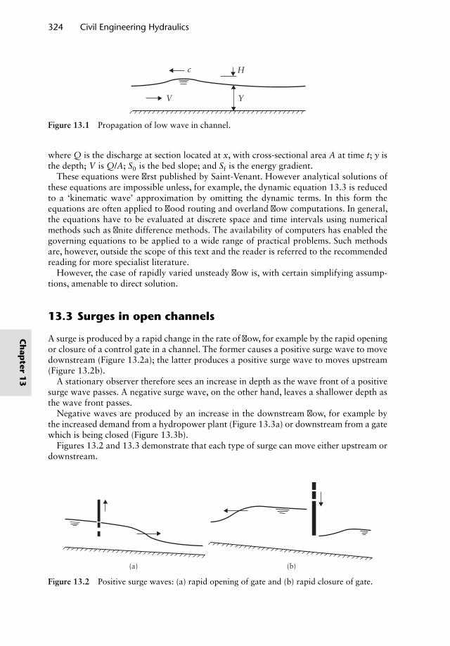
324 Civil Engineering Hydraulics
c
YV
H
Figure 13.1 Propagation of low wave in channel.
where Q is the discharge at section located at x, with cross-sectional area A at time t; y isthe depth; V is Q/A; S0 is the bed slope; and Sf is the energy gradient.
These equations were first published by Saint-Venant. However analytical solutions ofthese equations are impossible unless, for example, the dynamic equation 13.3 is reducedto a ‘kinematic wave’ approximation by omitting the dynamic terms. In this form theequations are often applied to flood routing and overland flow computations. In general,the equations have to be evaluated at discrete space and time intervals using numericalmethods such as finite difference methods. The availability of computers has enabled thegoverning equations to be applied to a wide range of practical problems. Such methodsare, however, outside the scope of this text and the reader is referred to the recommendedreading for more specialist literature.
However, the case of rapidly varied unsteady flow is, with certain simplifying assump-tions, amenable to direct solution.
13.3 Surges in open channels
A surge is produced by a rapid change in the rate of flow, for example by the rapid openingor closure of a control gate in a channel. The former causes a positive surge wave to movedownstream (Figure 13.2a); the latter produces a positive surge wave to moves upstream(Figure 13.2b).
A stationary observer therefore sees an increase in depth as the wave front of a positivesurge wave passes. A negative surge wave, on the other hand, leaves a shallower depth asthe wave front passes.
Negative waves are produced by an increase in the downstream flow, for example bythe increased demand from a hydropower plant (Figure 13.3a) or downstream from a gatewhich is being closed (Figure 13.3b).
Figures 13.2 and 13.3 demonstrate that each type of surge can move either upstream ordownstream.
(b)(a)
Figure 13.2 Positive surge waves: (a) rapid opening of gate and (b) rapid closure of gate.
Ch
apter
13
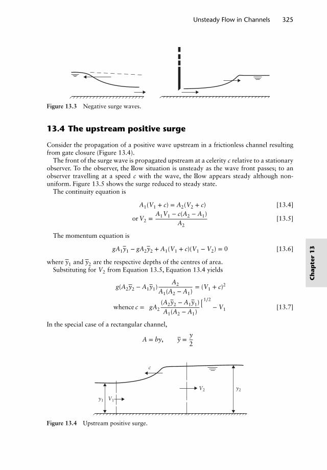
Unsteady Flow in Channels 325
Figure 13.3 Negative surge waves.
13.4 The upstream positive surge
Consider the propagation of a positive wave upstream in a frictionless channel resultingfrom gate closure (Figure 13.4).
The front of the surge wave is propagated upstream at a celerity c relative to a stationaryobserver. To the observer, the flow situation is unsteady as the wave front passes; to anobserver travelling at a speed c with the wave, the flow appears steady although non-uniform. Figure 13.5 shows the surge reduced to steady state.
The continuity equation is
A1(V1 + c) = A2(V2 + c) [13.4]
orV2 =A1V1 − c(A2 − A1)
A2[13.5]
The momentum equation is
gA1y1 − gA2y2 + A1(V1 + c)(V1 − V2) = 0 [13.6]
where y1 and y2 are the respective depths of the centres of area.Substituting for V2 from Equation 13.5, Equation 13.4 yields
g(A2y2 − A1y1)A2
A1(A2 − A1)= (V1 + c)2
whence c =[gA2
(A2y2 − A1y1)A1(A2 − A1)
]1∕2
− V1 [13.7]
In the special case of a rectangular channel,
A = by, y =y2
y1 V1
V2 y2
c
Figure 13.4 Upstream positive surge.
Ch
apte
r1
3
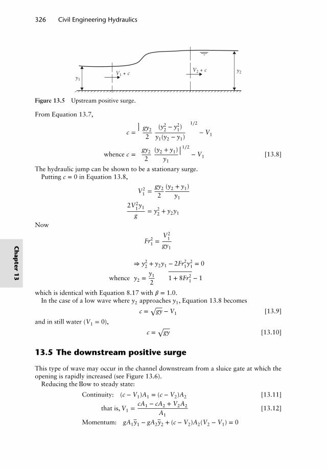
326 Civil Engineering Hydraulics
y1
y2V1 + cV2 + c
Figure 13.5 Upstream positive surge.
From Equation 13.7,
c =
[gy2
2
(y22 − y2
1)
y1(y2 − y1)
]1∕2
− V1
whence c =[
gy2
2(y2 + y1)
y1
]1∕2
− V1 [13.8]
The hydraulic jump can be shown to be a stationary surge.Putting c = 0 in Equation 13.8,
V21 =
gy2
2(y2 + y1)
y1
2V21y1
g= y2
2 + y2y1
Now
Fr21 =
V21
gy1
⇒ y22 + y2y1 − 2Fr2
1y21 = 0
whence y2 =y1
2
(√1 + 8Fr2
1 − 1)
which is identical with Equation 8.17 with 𝛽 = 1.0.In the case of a low wave where y2 approaches y1, Equation 13.8 becomes
c =√
gy − V1 [13.9]
and in still water (V1 = 0),
c =√
gy [13.10]
13.5 The downstream positive surge
This type of wave may occur in the channel downstream from a sluice gate at which theopening is rapidly increased (see Figure 13.6).
Reducing the flow to steady state:
Continuity: (c − V1)A1 = (c − V2)A2 [13.11]
that is, V1 =cA1 − cA2 + V2A2
A1[13.12]
Momentum: gA1y1 − gA2y2 + (c − V2)A2(V2 − V1) = 0
Ch
apter
13
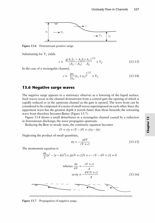
Unsteady Flow in Channels 327
y1
y2
c
V1
V2
Figure 13.6 Downstream positive surge.
Substituting for V1 yields
c =[
g(A1y1 − A2y2)(A1 − A2)
A1
A2
]1∕2
+ V2 [13.13]
In the case of a rectangular channel,
c =[
gy1
2y2(y1 + y2)
]1∕2
+ V2 [13.14]
13.6 Negative surge waves
The negative surge appears to a stationary observer as a lowering of the liquid surface.Such waves occur in the channel downstream from a control gate the opening of which israpidly reduced or in the upstream channel as the gate is opened. The wave front can beconsidered to be composed of a series of small waves superimposed on each other. Since theuppermost wave has the greatest depth it travels faster than those beneath; the retreatingwave front therefore becomes flatter (Figure 13.7).
Figure 13.8 shows a small disturbance in a rectangular channel caused by a reductionin downstream discharge; the wave propagates upstream.
Reducing the flow to steady state, the continuity equation becomes
(V + c)y = (V − 𝛿V + c)(y − 𝛿y)
Neglecting the product of small quantities,
𝛿y = −y𝛿V
(V + c)[13.15]
The momentum equation is
𝜌g2
[y2 − (y − 𝛿y)2] + 𝜌y(V + c){V + c − (V − 𝛿V + c)} = 0
whence𝛿y𝛿V
= − (V + c)g
or 𝛿y = −𝛿V(V + c)g
[13.16]
Figure 13.7 Propagation of negative surge.
Ch
apte
r1
3
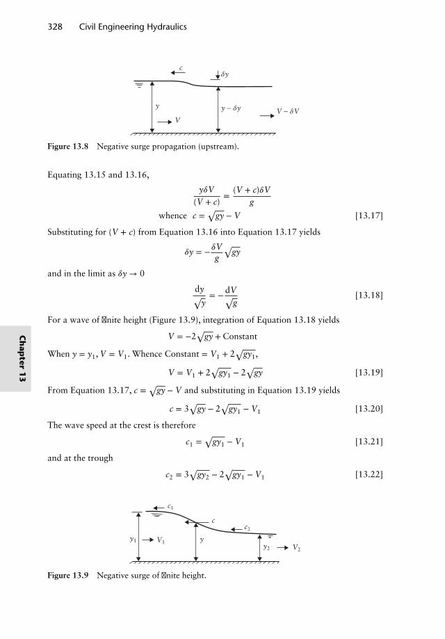
328 Civil Engineering Hydraulics
y
δy
y − δy V − δV V
c
Figure 13.8 Negative surge propagation (upstream).
Equating 13.15 and 13.16,
y𝛿V(V + c)
=(V + c)𝛿V
g
whence c =√
gy − V [13.17]
Substituting for (V + c) from Equation 13.16 into Equation 13.17 yields
𝛿y = −𝛿Vg
√gy
and in the limit as 𝛿y → 0
dy√y= − dV√
g[13.18]
For a wave of finite height (Figure 13.9), integration of Equation 13.18 yields
V = −2√
gy + Constant
When y = y1, V = V1. Whence Constant = V1 + 2√
gy1,
V = V1 + 2√
gy1 − 2√
gy [13.19]
From Equation 13.17, c =√
gy − V and substituting in Equation 13.19 yields
c = 3√
gy − 2√
gy1 − V1 [13.20]
The wave speed at the crest is therefore
c1 =√
gy1 − V1 [13.21]
and at the trough
c2 = 3√
gy2 − 2√
gy1 − V1 [13.22]
y1 V1V2y2
c2
c1
c
y
Figure 13.9 Negative surge of finite height.
Ch
apter
13
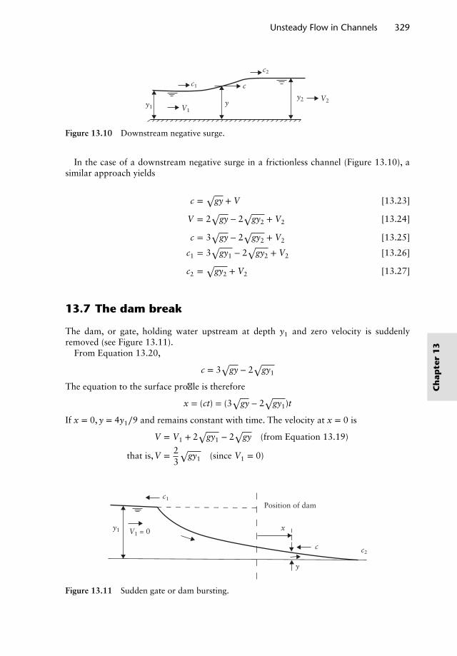
Unsteady Flow in Channels 329
y1 V1
V2y2
c
y
c1
c2
Figure 13.10 Downstream negative surge.
In the case of a downstream negative surge in a frictionless channel (Figure 13.10), asimilar approach yields
c =√
gy + V [13.23]
V = 2√
gy − 2√
gy2 + V2 [13.24]
c = 3√
gy − 2√
gy2 + V2 [13.25]
c1 = 3√
gy1 − 2√
gy2 + V2 [13.26]
c2 =√
gy2 + V2 [13.27]
13.7 The dam break
The dam, or gate, holding water upstream at depth y1 and zero velocity is suddenlyremoved (see Figure 13.11).
From Equation 13.20,
c = 3√
gy − 2√
gy1
The equation to the surface profile is therefore
x = (ct) = (3√
gy − 2√
gy1)t
If x = 0, y = 4y1∕9 and remains constant with time. The velocity at x = 0 is
V = V1 + 2√
gy1 − 2√
gy (from Equation 13.19)
that is,V = 23
√gy1 (since V1 = 0)
y1 V1 = 0
c
x
Position of dam
y
c1
c2
Figure 13.11 Sudden gate or dam bursting.
Ch
apte
r1
3
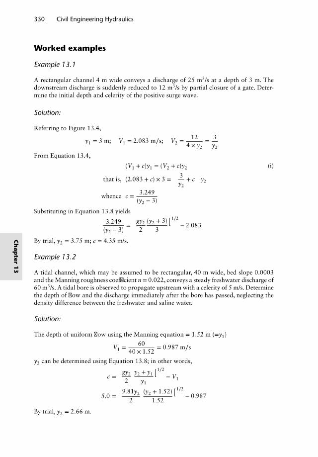
330 Civil Engineering Hydraulics
Worked examples
Example 13.1
A rectangular channel 4 m wide conveys a discharge of 25 m3/s at a depth of 3 m. Thedownstream discharge is suddenly reduced to 12 m3/s by partial closure of a gate. Deter-mine the initial depth and celerity of the positive surge wave.
Solution:
Referring to Figure 13.4,
y1 = 3 m; V1 = 2.083 m∕s; V2 = 124 × y2
= 3y2
From Equation 13.4,
(V1 + c)y1 = (V2 + c)y2 (i)
that is, (2.083 + c) × 3 =(
3y2
+ c)
y2
whence c = 3.249(y2 − 3)
Substituting in Equation 13.8 yields
3.249(y2 − 3)
=[
gy2
2(y2 + 3)
3
]1∕2
− 2.083
By trial, y2 = 3.75 m; c = 4.35 m/s.
Example 13.2
A tidal channel, which may be assumed to be rectangular, 40 m wide, bed slope 0.0003and the Manning roughness coefficient n = 0.022, conveys a steady freshwater discharge of60 m3/s. A tidal bore is observed to propagate upstream with a celerity of 5 m/s. Determinethe depth of flow and the discharge immediately after the bore has passed, neglecting thedensity difference between the freshwater and saline water.
Solution:
The depth of uniform flow using the Manning equation = 1.52 m (=y1)
V1 = 6040 × 1.52
= 0.987 m∕s
y2 can be determined using Equation 13.8; in other words,
c =[
gy2
2y2 + y1
y1
]1∕2
− V1
5.0 =[
9.81y2
2(y2 + 1.52)
1.52
]1∕2
− 0.987
By trial, y2 = 2.66 m.
Ch
apter
13
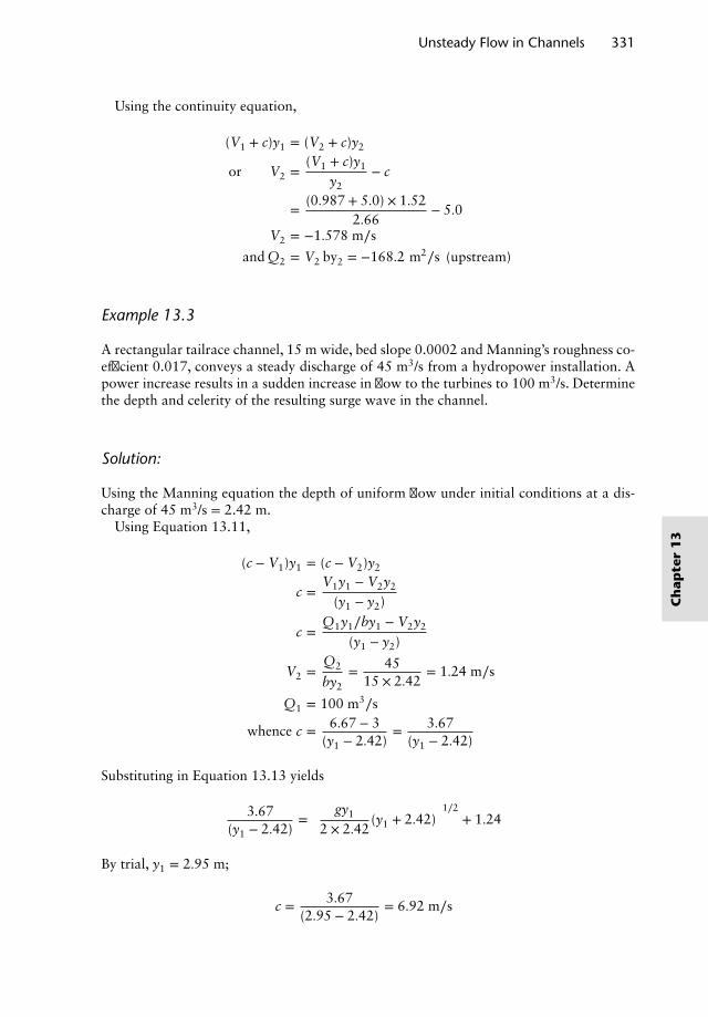
Unsteady Flow in Channels 331
Using the continuity equation,
(V1 + c)y1 = (V2 + c)y2
or V2 =(V1 + c)y1
y2− c
=(0.987 + 5.0) × 1.52
2.66− 5.0
V2 = −1.578 m∕s
and Q2 = V2 by2 = −168.2 m2∕s (upstream)
Example 13.3
A rectangular tailrace channel, 15 m wide, bed slope 0.0002 and Manning’s roughness co-efficient 0.017, conveys a steady discharge of 45 m3/s from a hydropower installation. Apower increase results in a sudden increase in flow to the turbines to 100 m3/s. Determinethe depth and celerity of the resulting surge wave in the channel.
Solution:
Using the Manning equation the depth of uniform flow under initial conditions at a dis-charge of 45 m3/s = 2.42 m.
Using Equation 13.11,
(c − V1)y1 = (c − V2)y2
c =V1y1 − V2y2
(y1 − y2)
c =Q1y1∕by1 − V2y2
(y1 − y2)
V2 =Q2
by2= 45
15 × 2.42= 1.24 m∕s
Q1 = 100 m3∕s
whence c = 6.67 − 3(y1 − 2.42)
= 3.67(y1 − 2.42)
Substituting in Equation 13.13 yields
3.67(y1 − 2.42)
=[ gy1
2 × 2.42(y1 + 2.42)
]1∕2+ 1.24
By trial, y1 = 2.95 m;
c = 3.67(2.95 − 2.42)
= 6.92 m∕s
Ch
apte
r1
3
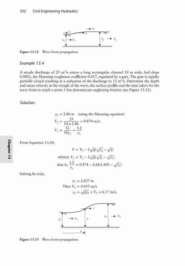
332 Civil Engineering Hydraulics
y1
c2c1
V1V2y2
c
Figure 13.12 Wave front propagation.
Example 13.4
A steady discharge of 25 m3/s enters a long rectangular channel 10 m wide, bed slope0.0001, the Manning roughness coefficient 0.017, regulated by a gate. The gate is rapidlypartially closed resulting in a reduction of the discharge to 12 m3/s. Determine the depthand mean velocity at the trough of the wave, the surface profile and the time taken for thewave front to reach a point 1 km downstream neglecting friction (see Figure 13.12).
Solution:
y2 = 2.86 m (using the Manning equation)
V2 = 2510 × 2.86
= 0.874 m∕s
V1 = 1210y1
= 1.2y1
From Equation 13.24,
V = V2 − 2√
g(√
y2 −√
y)
whence V1 = V2 − 2√
g(√
ys −√
y1)
that is, 1.2y1
= 0.874 − 6.26(1.691 −√
y1)
Solving by trial,
y1 = 2.637 m
Then V1 = 0.455 m∕s
c2 =√
gy2 + V2 = 6.17 m∕s
V1
V2y2y1
y
c
x
Figure 13.13 Wave front propagation.
Ch
apter
13
Unsteady Flow in Channels 333
Time taken to travel 1 km = 2.7 min.
Surface profile: x = ct = (3√
gy − 2√
gy2 + V2)t
or x = (9.4√
y − 10.6 + 0.874)t
x = (9.4√
y − 9.726)t.
References and recommended reading
Abbot, M. B. and Basco, D. R. (1989) Computational Fluid Dynamics, Longman, Harlow.Chadwick, A., Morfett, J. and Borthwick, M. (2013) Hydraulics in Civil and Environmental
Engineering, 5th edn, Spon, Abingdon, UK.Cunge, J. A., Holly, F. M. and Verwey, A. (1980) Practical Aspects of Computational River
Hydraulics, Pitman, London.French, R. H. (1994) Open Channel Hydraulics, 2nd edn, McGraw-Hill, New York.French, R. H. (2007) Open Channel Hydraulics, Water Resources Publications, Highlands
Ranch, CO.Henderson, F. M. (1966) Open Channel Flow, Macmillan, New York.Pickford, J. (1969) Analysis of Surge, Macmillan, London.
Problems
1. A rectangular channel 4 m wide conveys a discharge of 18 m3/s at a depth of 2.25 m.Determine the depth and celerity of the positive surge wave resulting from (a) suddenpartial gate closure which reduces the downstream discharge to 10 m3/s and (b) suddentotal gate closure.
2. At low tide the steady freshwater flow in an estuarial channel, 20 m wide, bed slope 0.0005and the Manning roughness coefficient 0.02, is 20 m3/s. A tidal bore forms on the floodtide and is observed to propagate upstream at a celerity of 4 m/s. Neglecting the densitydifference between the freshwater and the saline water, determine the depth and dischargeimmediately after the bore has passed.
3. A rectangular channel, 10 m wide, bed slope 0.0001 and the Manning roughness coefficient0.015, receives inflow from a reservoir with a gated inlet. When a steady discharge of 30m3/s is being conveyed, the gate is suddenly opened to release a discharge of 70 m3/s.Calculate the initial celerity and depth of the surge wave.
4. A steady discharge of 30 m3/s is conveyed in a rectangular channel of bed width 9 m at adepth of 3.0 m. A control gate at the inlet is suddenly partially closed reducing the inflowto 10 m3/s. Assuming the channel to be frictionless, determine the depth behind the surgewave and the time taken for the trough of the wave to pass a point 500 m downstream.
5. A rectangular channel 30 m wide discharges 60 m3/s at a uniform flow depth of 2.5 minto a reservoir. The levels of water in the channel and reservoir at the reservoir inlet areinitially equal. Water in the reservoir is released rapidly so that the level falls at the rate of1 m/h. Neglecting friction and the channel slope, determine the time taken for the level inthe channel to fall 0.5 m at a section 1 km upstream from the reservoir.
Ch
apte
r1
3

Chapter 14Uniform Flow inLoose-Boundary Channels
14.1 Introduction
The loose boundary (consisting of movable material) of a channel deforms under the actionof flowing water and the deformed bed with its changing roughness (bed forms) interactswith the flow. A dynamic equilibrium state of the boundary may be expected when a steadyand uniform flow has developed.
The resulting movement of the bed material (sediment) in the direction of flow is calledsediment transport and a certain critical bed shear stress (𝜏c) must be exceeded to start theparticle movement. Such a critical shear stress is referred to as the incipient (threshold)motion condition, below which the particles will be at rest and the flow is similar to thaton a rigid boundary.
14.2 Flow regimes
Shear stresses above the threshold condition disturb the initial plane boundary of the chan-nel, and the bed and water surface assume various forms depending on the sediment andfluid flow characteristics. Two distinct regimes of flow may be identified with the increasingflows with the following bed forms:
(a) Lower regime: ripples (for smaller sediment size <0.6 mm and low Froude number≪1), dunes and ripples, dunes with increasing shear (𝜏0) and Froude number Fr;further increases in 𝜏0 introduce transition to dunes/plane bed (Fr ≃ 1)
(b) Upper regime: flat bed, antidunes, chutes and pools with large shear and Froudenumbers (>1).
14.3 Incipient (threshold) motion
Shields (1936) introduced the concept of the dimensionless entrainment function(𝜏0∕𝜌gΔd) as a function of shear Reynolds number, Re∗ (=U∗d∕𝜈), where 𝜌 is density of
Nalluri & Featherstone’s Civil Engineering Hydraulics: Essential Theory with Worked Examples,Sixth Edition. Martin Marriott.© 2016 John Wiley & Sons, Ltd. Published 2016 by John Wiley & Sons, Ltd.Companion Website: www.wiley.com/go/Marriott
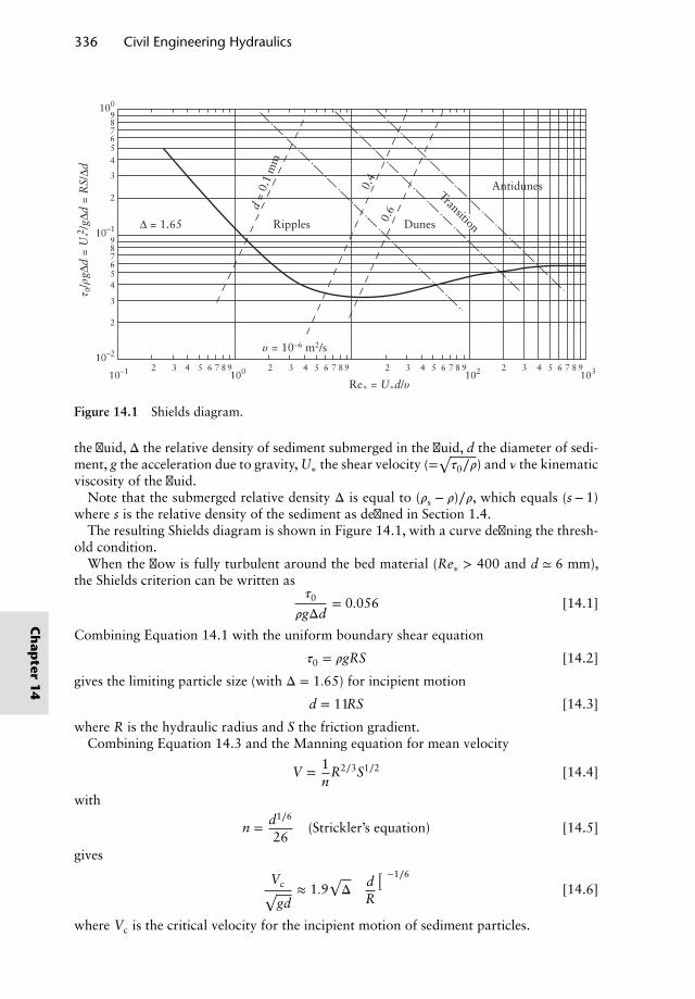
336 Civil Engineering Hydraulics
10–2
10–1 100 102 1032 3 4 5 6 7 8 9 2 3 4 5 6 7 8 9
Re* = U*d/υ
τ 0/ρ
gΔd
= U
*2 /gΔ
d =
RS/Δd
2 3 4 5 6 7 8 9 2 3 4 5 6 7 8 9
10–1
2
3
456789
100
2
3
456789
Δ = 1.65
υ = 10–6 m2/s
Ripples Dunes0.6
0.4
d =
0.1
mm
Antidunes
Transition
Figure 14.1 Shields diagram.
the fluid, Δ the relative density of sediment submerged in the fluid, d the diameter of sedi-ment, g the acceleration due to gravity, U∗ the shear velocity (=
√𝜏0∕𝜌) and 𝜈 the kinematic
viscosity of the fluid.Note that the submerged relative density Δ is equal to (𝜌s − 𝜌)∕𝜌, which equals (s−1)
where s is the relative density of the sediment as defined in Section 1.4.The resulting Shields diagram is shown in Figure 14.1, with a curve defining the thresh-
old condition.When the flow is fully turbulent around the bed material (Re∗ > 400 and d ≃ 6 mm),
the Shields criterion can be written as𝜏0
𝜌gΔd= 0.056 [14.1]
Combining Equation 14.1 with the uniform boundary shear equation
𝜏0 = 𝜌gRS [14.2]
gives the limiting particle size (with Δ = 1.65) for incipient motion
d = 11RS [14.3]
where R is the hydraulic radius and S the friction gradient.Combining Equation 14.3 and the Manning equation for mean velocity
V = 1n
R2∕3S1∕2 [14.4]
with
n = d1∕6
26(Strickler’s equation) [14.5]
gives
Vc√gd
≈ 1.9√Δ(
dR
)−1∕6
[14.6]
where Vc is the critical velocity for the incipient motion of sediment particles.
Ch
apter
14
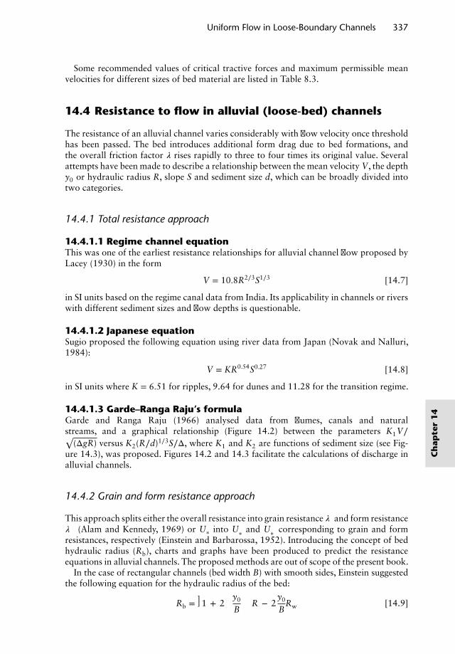
Uniform Flow in Loose-Boundary Channels 337
Some recommended values of critical tractive forces and maximum permissible meanvelocities for different sizes of bed material are listed in Table 8.3.
14.4 Resistance to flow in alluvial (loose-bed) channels
The resistance of an alluvial channel varies considerably with flow velocity once thresholdhas been passed. The bed introduces additional form drag due to bed formations, andthe overall friction factor 𝜆 rises rapidly to three to four times its original value. Severalattempts have been made to describe a relationship between the mean velocity V, the depthy0 or hydraulic radius R, slope S and sediment size d, which can be broadly divided intotwo categories.
14.4.1 Total resistance approach
14.4.1.1 Regime channel equationThis was one of the earliest resistance relationships for alluvial channel flow proposed byLacey (1930) in the form
V = 10.8R2∕3S1∕3 [14.7]
in SI units based on the regime canal data from India. Its applicability in channels or riverswith different sediment sizes and flow depths is questionable.
14.4.1.2 Japanese equationSugio proposed the following equation using river data from Japan (Novak and Nalluri,1984):
V = KR0.54S0.27 [14.8]
in SI units where K = 6.51 for ripples, 9.64 for dunes and 11.28 for the transition regime.
14.4.1.3 Garde–Ranga Raju’s formulaGarde and Ranga Raju (1966) analysed data from flumes, canals and naturalstreams, and a graphical relationship (Figure 14.2) between the parameters K1V∕√
(ΔgR) versus K2(R∕d)1∕3S∕Δ, where K1 and K2 are functions of sediment size (see Fig-ure 14.3), was proposed. Figures 14.2 and 14.3 facilitate the calculations of discharge inalluvial channels.
14.4.2 Grain and form resistance approach
This approach splits either the overall resistance into grain resistance 𝜆′ and form resistance𝜆′′ (Alam and Kennedy, 1969) or U∗ into U′
∗ and U′′∗ corresponding to grain and form
resistances, respectively (Einstein and Barbarossa, 1952). Introducing the concept of bedhydraulic radius (Rb), charts and graphs have been produced to predict the resistanceequations in alluvial channels. The proposed methods are out of scope of the present book.
In the case of rectangular channels (bed width B) with smooth sides, Einstein suggestedthe following equation for the hydraulic radius of the bed:
Rb =[1 + 2
(y0
B
)]R − 2
y0
BRw [14.9]
Ch
apte
r1
4
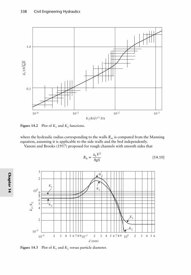
338 Civil Engineering Hydraulics
K2(R/d)1/3 S/Δ
K1V
/ Δg
R
10–4
0.1
1.0
10–3 10–2 10–1
Figure 14.2 Plot of K1 and K2 functions.
where the hydraulic radius corresponding to the walls Rw is computed from the Manningequation, assuming it is applicable to the side walls and the bed independently.
Vanoni and Brooks (1957) proposed for rough channels with smooth sides that
Rb =𝜆bV2
8gS[14.10]
10–2 10–1 100
3
2
987654
2
10–1
K2
d (mm)
K2
K2
K1
K1,
K2
K1
K1
100
2 3 4 5 6 7 89 2 3 4 5 6 7 89 2 3 4 5 6
Figure 14.3 Plot of K1 and K2 versus particle diameter.
Ch
apter
14
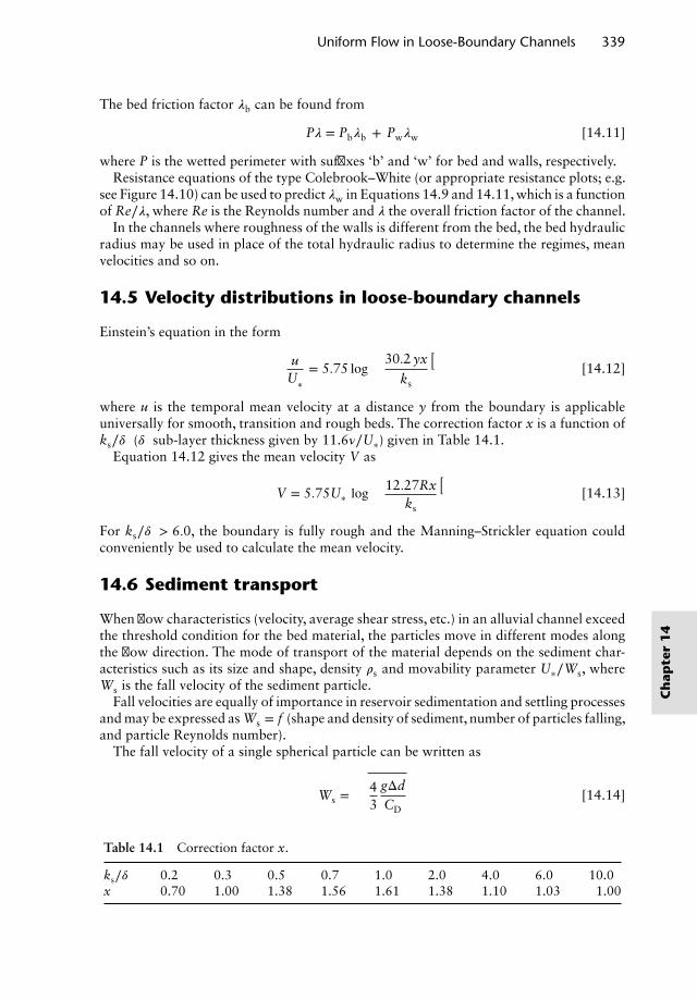
Uniform Flow in Loose-Boundary Channels 339
The bed friction factor 𝜆b can be found from
P𝜆 = Pb𝜆b + Pw𝜆w [14.11]
where P is the wetted perimeter with suffixes ‘b’ and ‘w’ for bed and walls, respectively.Resistance equations of the type Colebrook–White (or appropriate resistance plots; e.g.
see Figure 14.10) can be used to predict 𝜆w in Equations 14.9 and 14.11, which is a functionof Re∕𝜆, where Re is the Reynolds number and 𝜆 the overall friction factor of the channel.
In the channels where roughness of the walls is different from the bed, the bed hydraulicradius may be used in place of the total hydraulic radius to determine the regimes, meanvelocities and so on.
14.5 Velocity distributions in loose-boundary channels
Einstein’s equation in the form
uU′
∗= 5.75 log
(30.2 yx
ks
)[14.12]
where u is the temporal mean velocity at a distance y from the boundary is applicableuniversally for smooth, transition and rough beds. The correction factor x is a function ofks∕𝛿′ (𝛿′ sub-layer thickness given by 11.6𝜈∕U∗) given in Table 14.1.
Equation 14.12 gives the mean velocity V as
V = 5.75U∗ log(
12.27Rxks
)[14.13]
For ks∕𝛿′ > 6.0, the boundary is fully rough and the Manning–Strickler equation couldconveniently be used to calculate the mean velocity.
14.6 Sediment transport
When flow characteristics (velocity, average shear stress, etc.) in an alluvial channel exceedthe threshold condition for the bed material, the particles move in different modes alongthe flow direction. The mode of transport of the material depends on the sediment char-acteristics such as its size and shape, density 𝜌s and movability parameter U∗∕Ws, whereWs is the fall velocity of the sediment particle.
Fall velocities are equally of importance in reservoir sedimentation and settling processesand may be expressed as Ws = f (shape and density of sediment, number of particles falling,and particle Reynolds number).
The fall velocity of a single spherical particle can be written as
Ws =
√43
gΔdCD
[14.14]
Table 14.1 Correction factor x.
ks∕𝛿′ 0.2 0.3 0.5 0.7 1.0 2.0 4.0 6.0 10.0x 0.70 1.00 1.38 1.56 1.61 1.38 1.10 1.03 1.00
Ch
apte
r1
4
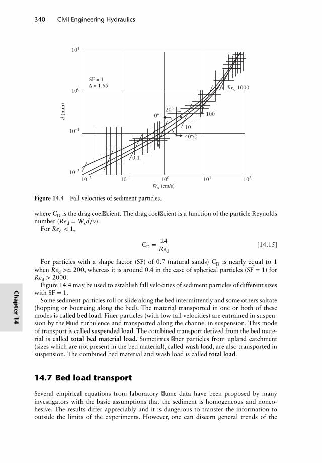
340 Civil Engineering Hydraulics
d (m
m)
100
101
10−1
10−2
10−2 10−1 100 101 102
100
10
40°C
0.1
0°20°
SF = 1
Red 1000
Ws (cm/s)
Δ = 1.65
Figure 14.4 Fall velocities of sediment particles.
where CD is the drag coefficient. The drag coefficient is a function of the particle Reynoldsnumber (Red = Wsd∕𝜈).
For Red < 1,
CD = 24Red
[14.15]
For particles with a shape factor (SF) of 0.7 (natural sands) CD is nearly equal to 1when Red >≃ 200, whereas it is around 0.4 in the case of spherical particles (SF = 1) forRed > 2000.
Figure 14.4 may be used to establish fall velocities of sediment particles of different sizeswith SF = 1.
Some sediment particles roll or slide along the bed intermittently and some others saltate(hopping or bouncing along the bed). The material transported in one or both of thesemodes is called bed load. Finer particles (with low fall velocities) are entrained in suspen-sion by the fluid turbulence and transported along the channel in suspension. This modeof transport is called suspended load. The combined transport derived from the bed mate-rial is called total bed material load. Sometimes finer particles from upland catchment(sizes which are not present in the bed material), called wash load, are also transported insuspension. The combined bed material and wash load is called total load.
14.7 Bed load transport
Several empirical equations from laboratory flume data have been proposed by manyinvestigators with the basic assumptions that the sediment is homogeneous and nonco-hesive. The results differ appreciably and it is dangerous to transfer the information tooutside the limits of the experiments. However, one can discern general trends of the
Ch
apter
14
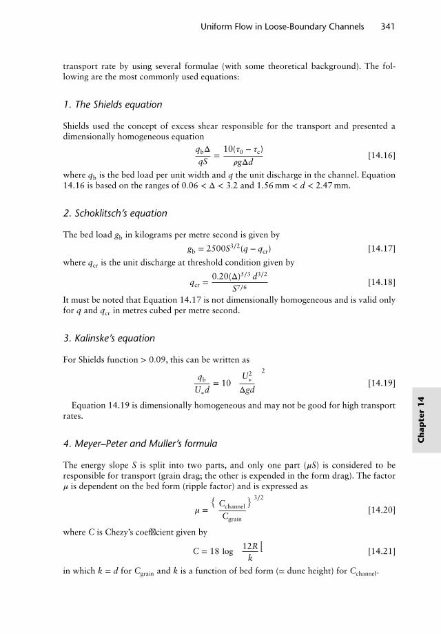
Uniform Flow in Loose-Boundary Channels 341
transport rate by using several formulae (with some theoretical background). The fol-lowing are the most commonly used equations:
1. The Shields equation
Shields used the concept of excess shear responsible for the transport and presented adimensionally homogeneous equation
qbΔqS
=10(𝜏0 − 𝜏c)
𝜌gΔd[14.16]
where qb is the bed load per unit width and q the unit discharge in the channel. Equation14.16 is based on the ranges of 0.06 < Δ < 3.2 and 1.56 mm < d < 2.47 mm.
2. Schoklitsch’s equation
The bed load gb in kilograms per metre second is given by
gb = 2500S3∕2(q − qcr) [14.17]
where qcr is the unit discharge at threshold condition given by
qcr =0.20(Δ)5∕3 d3∕2
S7∕6[14.18]
It must be noted that Equation 14.17 is not dimensionally homogeneous and is valid onlyfor q and qcr in metres cubed per metre second.
3. Kalinske’s equation
For Shields function > 0.09, this can be written as
qb
U∗d= 10
[U2
∗
Δgd
]2
[14.19]
Equation 14.19 is dimensionally homogeneous and may not be good for high transportrates.
4. Meyer–Peter and Muller’s formula
The energy slope S is split into two parts, and only one part (𝜇S) is considered to beresponsible for transport (grain drag; the other is expended in the form drag). The factor𝜇 is dependent on the bed form (ripple factor) and is expressed as
𝜇 =
(Cchannel
Cgrain
)3∕2
[14.20]
where C is Chezy’s coefficient given by
C = 18 log(
12Rk
)[14.21]
in which k = d for Cgrain and k is a function of bed form (≃ dune height) for Cchannel.
Ch
apte
r1
4
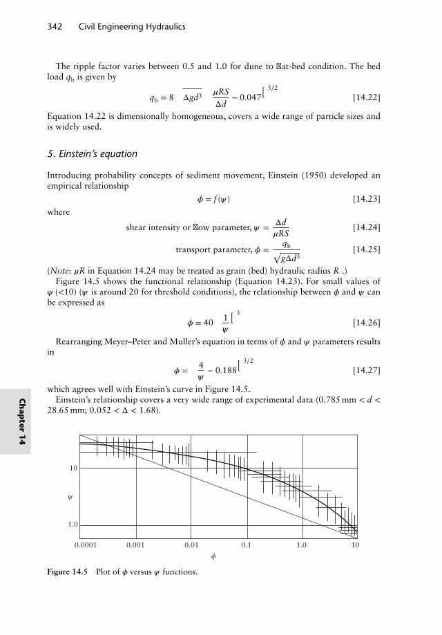
342 Civil Engineering Hydraulics
The ripple factor varies between 0.5 and 1.0 for dune to flat-bed condition. The bedload qb is given by
qb = 8√
Δgd3
(𝜇RSΔd
− 0.047)3∕2
[14.22]
Equation 14.22 is dimensionally homogeneous, covers a wide range of particle sizes andis widely used.
5. Einstein’s equation
Introducing probability concepts of sediment movement, Einstein (1950) developed anempirical relationship
𝜙 = f (𝜓) [14.23]
where
shear intensity or flow parameter, 𝜓 = Δd𝜇RS
[14.24]
transport parameter, 𝜙 =qb√gΔd3
[14.25]
(Note: 𝜇R in Equation 14.24 may be treated as grain (bed) hydraulic radius R′.)Figure 14.5 shows the functional relationship (Equation 14.23). For small values of
𝜓 (<10) (𝜓 is around 20 for threshold conditions), the relationship between 𝜙 and 𝜓 canbe expressed as
𝜙 = 40(
1𝜓
)3
[14.26]
Rearranging Meyer–Peter and Muller’s equation in terms of 𝜙 and 𝜓 parameters resultsin
𝜙 =(
4𝜓
− 0.188)3∕2
[14.27]
which agrees well with Einstein’s curve in Figure 14.5.Einstein’s relationship covers a very wide range of experimental data (0.785 mm < d <
28.65 mm; 0.052 < Δ < 1.68).
10
1.0
0.0001 0.001 0.01 0.1
ϕ
ψ
1.0 10
Figure 14.5 Plot of 𝜙 versus 𝜓 functions.
Ch
apter
14
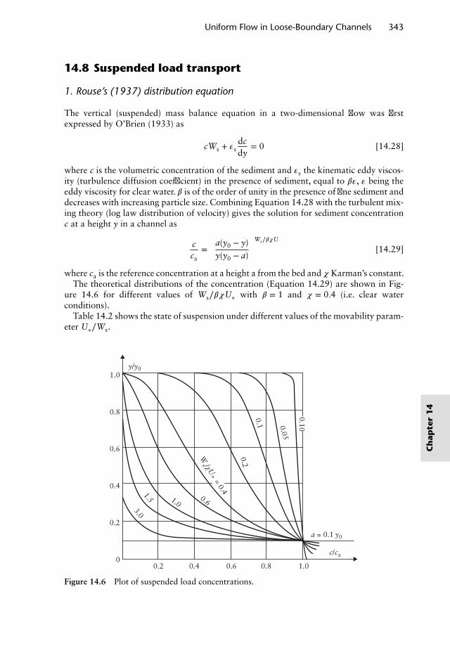
Uniform Flow in Loose-Boundary Channels 343
14.8 Suspended load transport
1. Rouse’s (1937) distribution equation
The vertical (suspended) mass balance equation in a two-dimensional flow was firstexpressed by O’Brien (1933) as
cWs + 𝜀sdcdy
= 0 [14.28]
where c is the volumetric concentration of the sediment and 𝜀s the kinematic eddy viscos-ity (turbulence diffusion coefficient) in the presence of sediment, equal to 𝛽𝜀, 𝜀 being theeddy viscosity for clear water. 𝛽 is of the order of unity in the presence of fine sediment anddecreases with increasing particle size. Combining Equation 14.28 with the turbulent mix-ing theory (log law distribution of velocity) gives the solution for sediment concentrationc at a height y in a channel as
cca
=[
a(y0 − y)y(y0 − a)
]Ws∕𝛽𝜒U
[14.29]
where ca is the reference concentration at a height a from the bed and 𝜒 Karman’s constant.The theoretical distributions of the concentration (Equation 14.29) are shown in Fig-
ure 14.6 for different values of Ws∕𝛽𝜒U∗ with 𝛽 = 1 and 𝜒 = 0.4 (i.e. clear waterconditions).
Table 14.2 shows the state of suspension under different values of the movability param-eter U∗∕Ws.
0.2
1.0
0.8
0.6
0.4
0.2
00.4 0.6 0.8 1.0
0.05
0.1
0.2
0.61.0
1.5
3.0
0.10
c/ca
Ws /χU
* = 0.4
y/y0
a = 0.1 y0
Figure 14.6 Plot of suspended load concentrations.
Ch
apte
r1
4
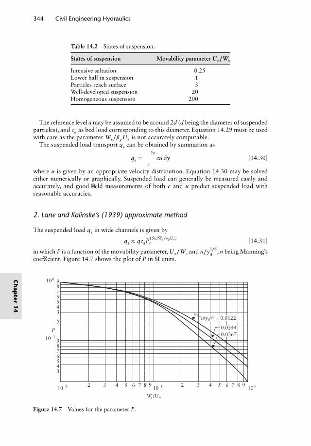
344 Civil Engineering Hydraulics
Table 14.2 States of suspension.
States of suspension Movability parameter U∗∕Ws
Intensive saltation 0.25Lower half in suspension 1Particles reach surface 3Well-developed suspension 20Homogeneous suspension 200
The reference level a may be assumed to be around 2d (d being the diameter of suspendedparticles), and ca as bed load corresponding to this diameter. Equation 14.29 must be usedwith care as the parameter Ws∕𝛽𝜒U∗ is not accurately computable.
The suspended load transport qs can be obtained by summation as
qs = ∫y0
acu dy [14.30]
where u is given by an appropriate velocity distribution. Equation 14.30 may be solvedeither numerically or graphically. Suspended load can generally be measured easily andaccurately, and good field measurements of both c and u predict suspended load withreasonable accuracies.
2. Lane and Kalinske’s (1939) approximate method
The suspended load qs in wide channels is given by
qs ≈ qcaP15(aWs∕y0U∗)e [14.31]
in which P is a function of the movability parameter, U∗∕Ws and n∕y1∕60 , n being Manning’s
coefficient. Figure 14.7 shows the plot of P in SI units.
9876543
9876543
2 3 4 5 6 7 8 9 2 3 4 5 6 7
0.03670.0244
n/y01/6 = 0.0122
8 910010−1
Ws /U*
10−2
10−1
100
2
P
Figure 14.7 Values for the parameter P.
Ch
apter
14
Uniform Flow in Loose-Boundary Channels 345
3. Empirical equations
Several practising engineers have reported several formulae of the type
qs ∝ qb [14.32]
the exponent b varying between 1.9 and 3.Engelund (1970) alternatively proposed that
qs = 0.5q(
U∗
Ws
)4
[14.33]
14.9 Total load transport
Total load includes both bed material load and wash load. Wash load is usually caused byland erosion, and a useful criterion for its existence may be taken as the particle Froudenumber (=V∕
√gd) around 20. Due to its small-size fractions, wash load moves in suspen-
sion and thus can be estimated from the total suspended load provided the suspended bedmaterial load is known. The following approaches describe some of the available directmethods of estimating the total bed material load.
1. Laursen’s (1958) approach
The cross-sectional mean concentration by volume Cv of the bed material load for quartzmaterial was suggested
Cv =160qb
q[14.34]
applicable to flume data with sand of d < 0.2 mm.
2. Garde’s (1968) equation
Field and flume data with the sediment size range of 0.011 mm < d < 0.93 mm gave
qt ≈ 10(
U∗
d3
)(RSΔ
)4
[14.35]
3. Graf’s approach
Similar to Einstein’s bed load equation, Graf (1984) used several flume and stream dataincluding closed conduit data to establish the equation
𝜙A = 10.39(𝜓A)−2.52 [14.36]
over a range of 10−2 < 𝜙 < 103, where
𝜙A =CvVR√
gΔd3[14.37]
and𝜓A = ΔdRS
[14.38]
Ch
apte
r1
4
346 Civil Engineering Hydraulics
Table 14.3 Coefficients in Equation 14.39.
Coefficient Fine and transitional Coarse
1.0 < dgr < 60 dgr > 60n n = 1.00 − 0.56 log dgr 0.00
Agr Agr = 0.14 + 0.23∕√
dgr 0.17
m m = 1.67 + 6.83∕dgr
C log C = 2.79 logdgr − 0.98(log dgr)2 − 3.46 0.025
4. Ackers–White’s formula
This method introduced by Ackers and White (1973) was updated by Ackers (1993) usingadditional data. The total sediment transport load is predicted from the equation:
qty0
qd
(U∗
V
)n
= C
(Fgr
Agr− 1
)m
[14.39]
where
Fgr =Un
∗√gΔd
[V√
32 log(10y0∕d)
]1−n
[14.40]
With the dimensionless grain diameter dgr defined by
dgr = d[
gΔ𝜈2
]1∕3
[14.41]
the coefficients in Equation 14.39 are shown in Table 14.3.
14.10 Regime channel design
1. Kennedy’s approach
Regime equations were developed using data from stable channels in the Indian subconti-nent, carrying moderate sediment loads of less than 500 ppm by weight. These equationsdo not consider sediment load variable and have limitations due to the fact that they areapplicable to boundary characteristics similar to those found in the Indian subcontinent.
Kennedy’s equation for nonsilting and nonscouring velocities V is given by
V = 0.55my0.640 [14.42]
where y0 is the flow depth in metres and V is in metres per second; m is the critical velocityratio (=V∕V0), a function of the sand size (m = 1 for the standard size, d ≈ 0.323 mm).Table 14.4 shows m values for other sand sizes.
Equation 14.42 combined with the Manning equation (Equation 8.4b) gives two equa-tions (Ranga Raju, 1993):
y0 =[
1.818Q(p + 0.5)m
]0.378
[14.43]
Ch
apter
14
Uniform Flow in Loose-Boundary Channels 347
Table 14.4 m values as a function of sand size.
Type of sand m Remark
Fine silt 0.7Light sand silt 1.0 Standard size (data)Coarse sand silt 1.1Sand loamy silt 1.2Coarser silt 1.3
where p = b∕y0, b being the bed width of a trapezoidal channel with side slopes of 0.5(horizontal) : 1 (vertical) (the final shape of the regime channel is not truly trapezoidal,and the final side slopes are much steeper due to silt deposition on banks), and
SQ0.02
n2m2= 0.3
[(p + 2.236)4∕3
(p + 0.5)1.31
][14.44]
Equations 14.43 and 14.44 give any number of solutions for the three unknowns, b, y0 andthe slope S for given values of Q, m and Manning’s n. Usually, the bed slope is assumed tobe a reasonable value (based on past experience and surrounding terrain slope), and p andy0, and hence b, are computed. Table 14.5 alternatively suggests the recommended valuesof p for stable channels as a function of Q.
2. Lacey’s approach
Lacey proposed the following equations (Kennedy’s equation does not specify the channelwidth, and experience suggests that this is an important parameter) for regime channeldesign:
P = 4.75√
Q [14.45]
R = 0.47(
Q
f
)1∕3
[14.46]
S = 3 × 10⁻⁴ f 5∕3
Q1∕6[14.47]
in which the silt factor f is given by
f = 1.76√
d [14.48]
where d is in millimetres, P and R are in metres and Q is in metres cubed per second.The silt factor f is a function of its size, as indicated in Table 14.6. Combining Equations14.45–14.47, Lacey suggested the resistance equation
V = 10.8R2∕3S1∕3 [14.49]
Table 14.5 Recommended b∕y0 values.
Q (m3/s) 5.0 10.0 15.0 50.0 100.0 200.0 300.0p (=b∕y0) 4.5 5.0 6.5 9.0 12.0 15.0 18.0
Ch
apte
r1
4
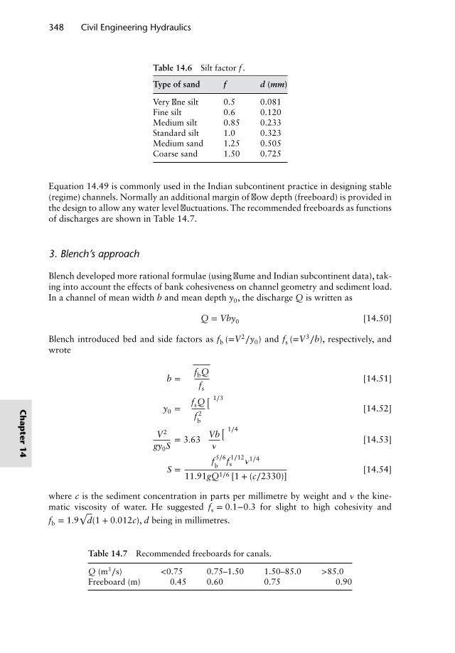
348 Civil Engineering Hydraulics
Table 14.6 Silt factor f .
Type of sand f d (mm)
Very fine silt 0.5 0.081Fine silt 0.6 0.120Medium silt 0.85 0.233Standard silt 1.0 0.323Medium sand 1.25 0.505Coarse sand 1.50 0.725
Equation 14.49 is commonly used in the Indian subcontinent practice in designing stable(regime) channels. Normally an additional margin of flow depth (freeboard) is provided inthe design to allow any water level fluctuations. The recommended freeboards as functionsof discharges are shown in Table 14.7.
3. Blench’s approach
Blench developed more rational formulae (using flume and Indian subcontinent data), tak-ing into account the effects of bank cohesiveness on channel geometry and sediment load.In a channel of mean width b and mean depth y0, the discharge Q is written as
Q = Vby0 [14.50]
Blench introduced bed and side factors as fb (=V2∕y0) and fs (=V3∕b), respectively, andwrote
b =
√fbQ
fs[14.51]
y0 =(
fsQ
f 2b
)1∕3
[14.52]
V2
gy0S= 3.63
(Vb𝜈
)1∕4
[14.53]
S =f 5∕6b
f 1∕12s 𝜈1∕4
11.91gQ1∕6 [1 + (c∕2330)][14.54]
where c is the sediment concentration in parts per millimetre by weight and 𝜈 the kine-matic viscosity of water. He suggested fs = 0.1−0.3 for slight to high cohesivity and
fb = 1.9√
d(1 + 0.012c), d being in millimetres.
Table 14.7 Recommended freeboards for canals.
Q (m3∕s) <0.75 0.75–1.50 1.50–85.0 >85.0Freeboard (m) 0.45 0.60 0.75 0.90
Ch
apter
14
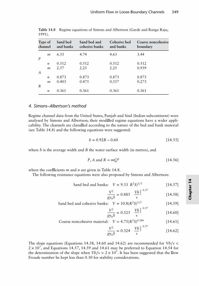
Uniform Flow in Loose-Boundary Channels 349
Table 14.8 Regime equations of Simons and Albertson (Garde and Ranga Raju,1991).
Type of Sand bed Sand bed and Cohesive bed Coarse noncohesivechannel and banks cohesive banks and banks boundary
m 6.33 4.74 4.63 3.44P
n 0.512 0.512 0.512 0.512m 2.57 2.25 2.25 0.939
An 0.873 0.873 0.873 0.873m 0.403 0.475 0.557 0.273
Rn 0.361 0.361 0.361 0.361
4. Simons–Albertson’s method
Regime channel data from the United States, Punjab and Sind (Indian subcontinent) wereanalysed by Simons and Albertson; their modified regime equations have a wider appli-cability. The channels are classified according to the nature of the bed and bank material(see Table 14.8) and the following equations were suggested:
b = 0.92B − 0.60 [14.55]
where b is the average width and B the water surface width (in metres), and
P, A and R = mQn [14.56]
where the coefficients m and n are given in Table 14.8.The following resistance equations were also proposed by Simons and Albertson:
Sand bed and banks: V = 9.33(R2S)1∕3 [14.57]
V2
gy0S= 0.885
(Vb𝜈
)0.37
[14.58]
Sand bed and cohesive banks: V = 10.8(R2S)1∕3 [14.59]
V2
gy0S= 0.525
(Vb𝜈
)0.37
[14.60]
Coarse noncohesive material: V = 4.75(R2S)0.286 [14.61]
V2
gy0S= 0.324
(Vb𝜈
)0.37
[14.62]
The slope equations (Equations 14.58, 14.60 and 14.62) are recommended for Vb∕𝜈 <2 × 10⁷, and Equations 14.57, 14.59 and 14.61 may be preferred to Equation 14.54 forthe determination of the slope when Vb∕𝜈 > 2 × 10⁷. It has been suggested that the flowFroude number be kept less than 0.30 for stability considerations.
Ch
apte
r1
4
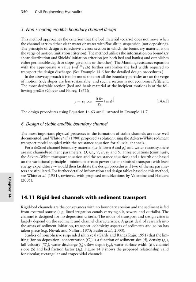
350 Civil Engineering Hydraulics
5. Non-scouring erodible boundary channel design
This method approaches the criterion that the bed material (coarse) does not move whenthe channel carries either clear water or water with fine silt in suspension (not depositing).The principle of design is to achieve a cross section in which the boundary material is onthe verge of motion (initiation criterion). The method utilises the information on boundaryshear distribution and Shields’ initiation criterion (on both bed and banks) and establisheseither permissible depth or slope (given one or the other). The Manning resistance equationwith the appropriate n value (=d1∕6∕26) further establishes the bed width required totransport the design discharge. (See Example 14.6 for the detailed design procedures.)
In the above approach it is to be noted that not all the boundary particles are on the vergeof motion (side slopes are less sustainable) and such a section is not economical/efficient.The most desirable section (bed and bank material at the incipient motion) is of the fol-lowing profile (Glover and Florey, 1951):
y = y0 cos(
0.8xy0
tan𝜙)
[14.63]
The design procedures using Equation 14.63 are illustrated in Example 14.7.
6. Design of stable erodible boundary channel
The most important physical processes in the formation of stable channels are now welldocumented, and White et al. (1980) proposed a solution using the Ackers–White sedimenttransport model coupled with the resistance equation for alluvial channels.
For a defined channel boundary material (i.e. known d and 𝜌s) and water viscosity, thereare six channel/sediment parameters: Q, Qs, V, B, y0 and S. Three equations (continuity,the Ackers–White transport equation and the resistance equation) and a fourth one basedon the variational principle – minimum stream power (i.e. maximised transport with leastenergy expenditure) – would then facilitate the design procedures if two of the six parame-ters are stipulated. For further detailed information and design tables based on this method,see White et al. (1981), reviewed with proposed modifications by Valentine and Haidera(2005).
14.11 Rigid-bed channels with sediment transport
Rigid-bed channels are the conveyances with no boundary erosion and the sediment is fedfrom external source (e.g. lined irrigation canals carrying silt, sewers and outfalls). Thechannel is designed for no deposition criteria. The mode of transport and design criterialargely depend on the sediment and channel characteristics. A great deal of research intothe areas of sediment initiation, transport, cohesivity aspects of sediments and so on hastaken place (e.g. Novak and Nalluri, 1975; Butler et al., 2003).
Studies of noncohesive suspended silt reveal (Garde and Ranga Raju, 1991) that the lim-iting (for no deposition) concentration (Cv) is a function of sediment size (d), density (𝜌s),fall velocity (Ws), water discharge (Q), flow depth (y0), water surface width (B), channelslope (S) and bed friction factor (𝜆b). Figure 14.8 shows the proposed relationship validfor circular, rectangular and trapezoidal channels.
Ch
apter
14
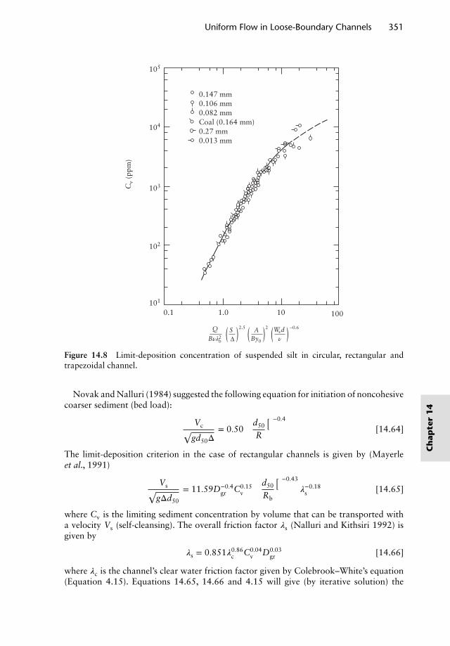
Uniform Flow in Loose-Boundary Channels 351
0.147 mm0.106 mm0.082 mmCoal (0.164 mm)0.27 mm0.013 mm
105
104
103
102
101
0.1 1.0
Q SBνλb
2
2.5 2 −0.6
νBy0( )( )( ) Wsd
ΔA
10 100
Cv
(ppm
)
Figure 14.8 Limit-deposition concentration of suspended silt in circular, rectangular andtrapezoidal channel.
Novak and Nalluri (1984) suggested the following equation for initiation of noncohesivecoarser sediment (bed load):
Vc√gd50Δ
= 0.50(
d50
R
)−0.4
[14.64]
The limit-deposition criterion in the case of rectangular channels is given by (Mayerleet al., 1991)
Vs√gΔd50
= 11.59D−0.4gr C0.15
v
(d50
Rb
)−0.43
𝜆−0.18s [14.65]
where Cv is the limiting sediment concentration by volume that can be transported witha velocity Vs (self-cleansing). The overall friction factor 𝜆s (Nalluri and Kithsiri 1992) isgiven by
𝜆s = 0.851𝜆0.86c C0.04
v D0.03gr [14.66]
where 𝜆c is the channel’s clear water friction factor given by Colebrook–White’s equation(Equation 4.15). Equations 14.65, 14.66 and 4.15 will give (by iterative solution) the
Ch
apte
r1
4
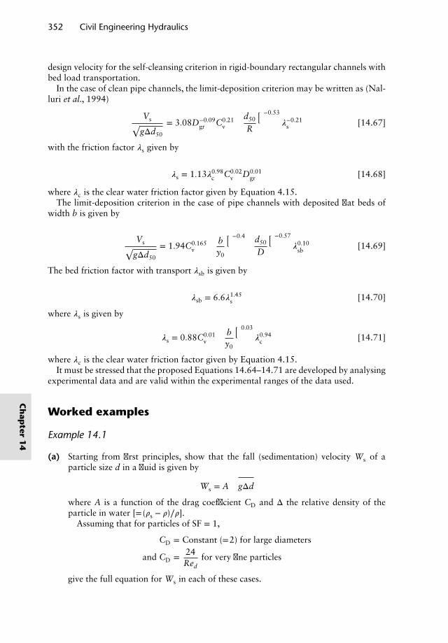
352 Civil Engineering Hydraulics
design velocity for the self-cleansing criterion in rigid-boundary rectangular channels withbed load transportation.
In the case of clean pipe channels, the limit-deposition criterion may be written as (Nal-luri et al., 1994)
Vs√gΔd50
= 3.08D−0.09gr C0.21
v
(d50
R
)−0.53
𝜆−0.21s [14.67]
with the friction factor 𝜆s given by
𝜆s = 1.13𝜆0.98c C0.02
v D0.01gr [14.68]
where 𝜆c is the clear water friction factor given by Equation 4.15.The limit-deposition criterion in the case of pipe channels with deposited flat beds of
width b is given by
Vs√gΔd50
= 1.94C0.165v
(by0
)−0.4 (d50
D
)−0.57
𝜆0.10sb
[14.69]
The bed friction factor with transport 𝜆sb is given by
𝜆sb = 6.6𝜆1.45s [14.70]
where 𝜆s is given by
𝜆s = 0.88C0.01v
(by0
)0.03
𝜆0.94c [14.71]
where 𝜆c is the clear water friction factor given by Equation 4.15.It must be stressed that the proposed Equations 14.64–14.71 are developed by analysing
experimental data and are valid within the experimental ranges of the data used.
Worked examples
Example 14.1
(a) Starting from first principles, show that the fall (sedimentation) velocity Ws of aparticle size d in a fluid is given by
Ws = A√
gΔd
where A is a function of the drag coefficient CD and Δ the relative density of theparticle in water [= (𝜌s − 𝜌)∕𝜌].
Assuming that for particles of SF = 1,
CD = Constant (=2) for large diameters
and CD = 24Red
for very fine particles
give the full equation for Ws in each of these cases.
Ch
apter
14
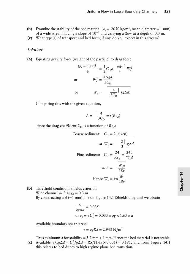
Uniform Flow in Loose-Boundary Channels 353
(b) Examine the stability of the bed material (𝜌s = 2650 kg/m3, mean diameter = 1 mm)of a wide stream having a slope of 10−3 and carrying a flow at a depth of 0.3 m.
(c) What type(s) of transport and bed form, if any, do you expect in this stream?
Solution:
(a) Equating gravity force (weight of the particle) to drag force
(𝜌s − 𝜌)g𝜋d3
6= 1
2CD𝜌
(𝜋d2
4
)W2
s
or W2s =
4Δgd3CD
or Ws =
√(4
3CD
)(gΔd)
Comparing this with the given equation,
A =
√4
3CD= f (Red)
since the drag coefficient CD is a function of Red:
Coarse sediment: CD = 2 (given)
⇒ Ws =
√(23
)gΔd
Fine sediment: CD = 24Red
= 24𝜈Wsd
⇒ A =
√Wsd18𝜈
Hence Ws = gΔ d2
18𝜈
(b) Threshold condition: Shields criterionWide channel ⇒ R ≈ y0 = 0.3 mBy constructing a d (=1 mm) line on Figure 14.1 (Shields diagram) we obtain
𝜏c
𝜌gΔd= 0.035
or 𝜏c = 𝜌U2∗ = 0.035 × 𝜌g × 1.65 × d
Available boundary shear stress
𝜏 = 𝜌gRS = 2.943 N∕m2
Thus minimum d for stability = 5.2 mm > 1 mm. Hence the bed material is not stable.(c) Available 𝜏∕𝜌gΔd = U2
∗∕gΔd = RS∕(1.65 × 0.001) = 0.181, and from Figure 14.1this relates to bed dunes to high regime plane bed transition.
Ch
apte
r1
4
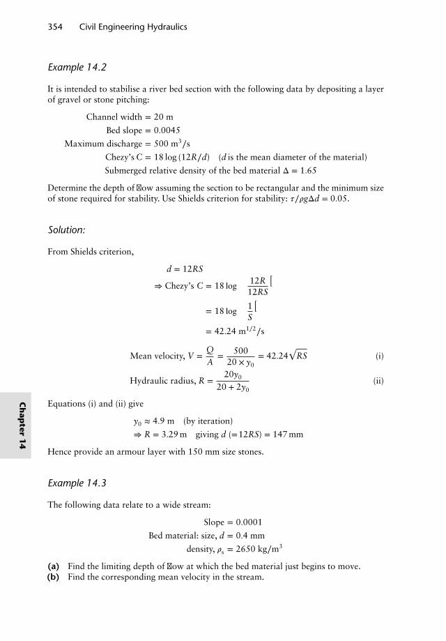
354 Civil Engineering Hydraulics
Example 14.2
It is intended to stabilise a river bed section with the following data by depositing a layerof gravel or stone pitching:
Channel width = 20 m
Bed slope = 0.0045
Maximum discharge = 500 m3∕s
Chezy’s C = 18 log (12R∕d) (d is the mean diameter of the material)
Submerged relative density of the bed material Δ = 1.65
Determine the depth of flow assuming the section to be rectangular and the minimum sizeof stone required for stability. Use Shields criterion for stability: 𝜏∕𝜌gΔd = 0.05.
Solution:
From Shields criterion,
d = 12RS
⇒ Chezy’s C = 18 log(
12R12RS
)
= 18 log(
1S
)= 42.24 m1∕2∕s
Mean velocity, V =QA
= 50020 × y0
= 42.24√
RS (i)
Hydraulic radius, R =20y0
20 + 2y0(ii)
Equations (i) and (ii) give
y0 ≈ 4.9 m (by iteration)
⇒ R = 3.29 m giving d (=12RS) = 147 mm
Hence provide an armour layer with 150 mm size stones.
Example 14.3
The following data relate to a wide stream:
Slope = 0.0001
Bed material: size, d = 0.4 mm
density, 𝜌s = 2650 kg∕m3
(a) Find the limiting depth of flow at which the bed material just begins to move.(b) Find the corresponding mean velocity in the stream.
Ch
apter
14
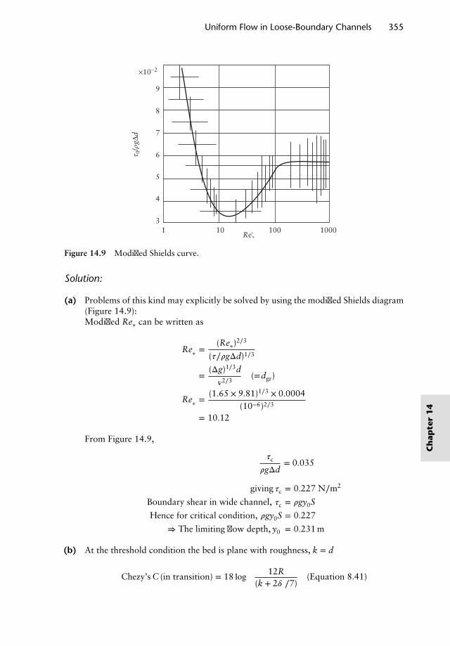
Uniform Flow in Loose-Boundary Channels 355
9
8
7
6
5
4
3
×10−2
τ 0/ρ
gΔd
1 10 100 1000Re*
Figure 14.9 Modified Shields curve.
Solution:
(a) Problems of this kind may explicitly be solved by using the modified Shields diagram(Figure 14.9):Modified Re∗ can be written as
Re′∗ =(Re∗)
2∕3
(𝜏∕𝜌gΔd)1∕3
=(Δg)1∕3d
𝜈2∕3(=dgr)
Re′∗ = (1.65 × 9.81)1∕3 × 0.0004(10−6)2∕3
= 10.12
From Figure 14.9,
𝜏c
𝜌gΔd= 0.035
giving 𝜏c = 0.227 N∕m2
Boundary shear in wide channel, 𝜏c = 𝜌gy0S
Hence for critical condition, 𝜌gy0S = 0.227
⇒ The limiting flow depth, y0 = 0.231 m
(b) At the threshold condition the bed is plane with roughness, k = d
Chezy’s C (in transition) = 18 log[
12R(k + 2𝛿′∕7)
](Equation 8.41)
Ch
apte
r1
4
356 Civil Engineering Hydraulics
where 𝛿′ is the sub-layer thickness given by 𝛿′ = 11.6𝜈∕U∗.
k = d = 0.0004 m, 𝛿′ = 11.6 × 10⁻⁶√9.81 × 0.231 × 0.0001
= 7.7 × 10⁻⁵ m
⇒ k + 2𝛿′
7= 0.0004 + 0.000022 = 0.000422 m
⇒ C = 18 log(
12 × 0.2310.000422
)= 54.7 m1∕2∕s
Hence mean velocity, V = C√
RS
= 54.7 ×√
0.231 × 0.0001
= 0.263 m∕s
Example 14.4
A wide alluvial stream carries water with a mean depth of 1 m and slope of 0.0005. Themean diameter of the bed material is 0.5 mm with a relative density of 2.65. Examine thebed stability and bed form, if any. Also calculate the sediment transport rate that may existin the channel.
Solution:
Wide channel ⇒ R ≈ y0 = 1.0 m; S = 0.0005; d = 0.0005 m⇒ dgr = 12.5
From Figure 14.9,
𝜏
𝜌gΔd= 0.32
⇒ 𝜏c = 0.032 × 1000 × 9.81 × 1.65 × 0.0005
= 0.234 N∕m2
Channel boundary shear stress, 𝜏0 = 𝜌gRS = 4.9 N/m2
Since 𝜏0 > 𝜏c, sediment transport exists.
Type of transport:Fall velocity of sediment particle from Figure 14.4
Ws = 0.075 m∕s
⇒ Movability parameter,U∗
Ws= 0.93
Referring to Table 14.2, most part of the transport may be treated as bed load whichmay be computed using Shields’ equation (Equation 14.16).
Ch
apter
14
Uniform Flow in Loose-Boundary Channels 357
Discharge computations:Referring to Garde and Ranga Raju’s plots (Figures 14.2 and 14.3), mean velocity in the
channel may be determined.
For d = 0.5 mm; K1 = K2 = 0.95 (Figure 14.3)
⇒ K2
(Rd
)1∕3 SΔ
= 3.63 × 10⁻³
From Figure 14.2,
K1V√gΔR
= 0.20
Hence V = 0.847 m/s, giving q = Vy0 = 0.847 m3/(m s).From Shields’ equation 14.19, the bed load transport
qb =10(𝜏0 − 𝜏c) qS
𝜌gΔ2d
= 10 × (4.9 − 0.292) × 0.847 × 0.00051000 × 9.81 × 1.652 × 0.0005
= 1.46 × 10⁻³ m3∕(m s)
≈ 40 N/(m s) or 4 kg/(m s)
Bed form:
𝜏0
𝜌gΔd= 4.9
1000 × 9.81 × 1.65 × 0.0005= 0.61
From Shields’ curve (Figure 14.1), the bed form may be in high regime transition toantidunes; however, the flow Froude number (=V∕
√gy0) is less than 1 and the bed may
be in dune to high regime transition form.Equivalent bed roughness (k) or dune height:
Using Chezy’s equation, V = C√
(RS)
Chezy’s C = 0.847∕√
(1 × 0.0005) = 37.88 m1∕2
Hence from C = 18 log (12R∕k) (assuming fully rough bed)
k = 9.5 × 10⁻² m or 95 mm
Example 14.5
A laboratory rectangular flume with smooth sides and rough alluvial bed (d = 6.5 mm) ofthe following data carries 0.1 m3/s of water:
Bed width = 0.5 m
Depth of flow = 0.25 m
Slope = 3 × 10⁻³
Find the bed hydraulic radius using the resistance curve for smooth sides (Figure 14.9),bed shear stress and Manning’s coefficient. Also examine the stability of the bed.
Ch
apte
r1
4
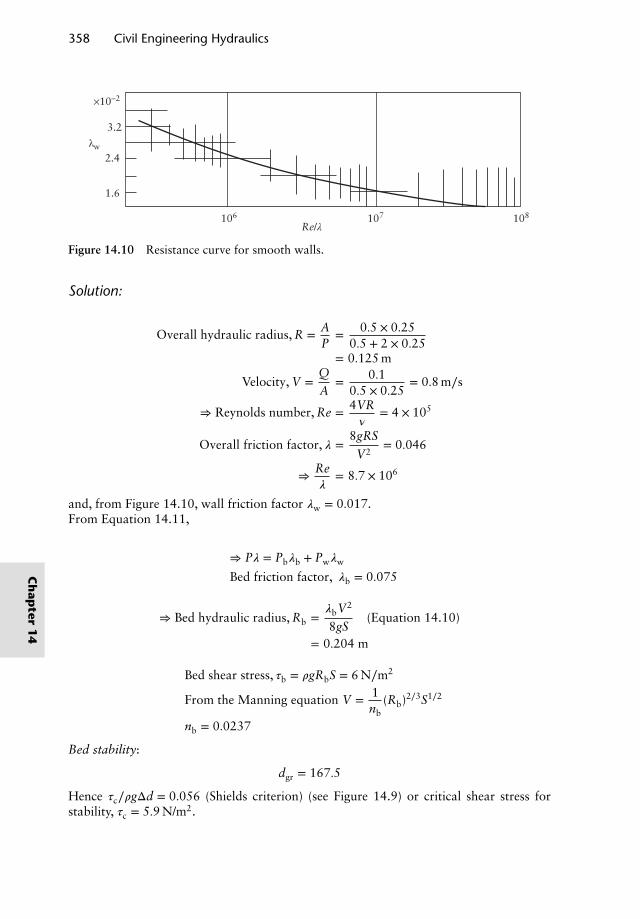
358 Civil Engineering Hydraulics
3.2
2.4
1.6
×10−2
106 107 108
λw
Re/λ
Figure 14.10 Resistance curve for smooth walls.
Solution:
Overall hydraulic radius, R = AP
= 0.5 × 0.250.5 + 2 × 0.25
= 0.125 m
Velocity, V =QA
= 0.10.5 × 0.25
= 0.8 m∕s
⇒ Reynolds number, Re = 4VR𝜈
= 4 × 10⁵
Overall friction factor, 𝜆 =8gRS
V2= 0.046
⇒Re𝜆
= 8.7 × 10⁶
and, from Figure 14.10, wall friction factor 𝜆w = 0.017.From Equation 14.11,
⇒ P𝜆 = Pb𝜆b + Pw𝜆w
Bed friction factor, 𝜆b = 0.075
⇒ Bed hydraulic radius, Rb =𝜆bV2
8gS(Equation 14.10)
= 0.204 m
Bed shear stress, 𝜏b = 𝜌gRbS = 6 N∕m2
From the Manning equation V = 1nb
(Rb)2∕3S1∕2
nb = 0.0237
Bed stability:
dgr = 167.5
Hence 𝜏c∕𝜌gΔd = 0.056 (Shields criterion) (see Figure 14.9) or critical shear stress forstability, 𝜏c = 5.9 N/m2.
Ch
apter
14
Uniform Flow in Loose-Boundary Channels 359
As 𝜏b ≃ 𝜏c, the bed is just stable.Note: Overall Manning’s n = R2∕3S1∕2∕V = 0.017, which may be compared with Strick-
ler’s equation giving n = d1∕6∕26 = 0.0166 with k = d.
Example 14.6
Design a stable alluvial channel of trapezoidal cross section with the following data:
Discharge = 50 m3∕s
Bed material size = 4 mm
Angle of repose, 𝜙 = 30◦
Bed slope = 10−4
Channel side slopes = 2 (horizontal) : 1 (vertical)(tan 𝜃 = 1
2
)
Solution:
Re′∗ =(Δg)1∕3d
𝜈2∕3= 100.8
From Figure 14.9,
Fr2d = 𝜏
𝜌gΔd= 0.054
⇒ Critical bed shear stress, 𝜏bc = 0.054 × 1000 × 9.81 × 1.65 × 0.004
= 3.496 N∕m2
Hence critical shear on slopes, 𝜏sc = K𝜏bc
where K =(
1 − sin2𝜃
sin2𝜙
)1∕2
=(
1 − 0.20.25
)1∕2
= 0.447
⇒ 𝜏sc = 0.447 × 3.496 = 1.563 N∕m2
Mean boundary shear distribution in a 2 (horizontal) : 1 (vertical) trapezoidal channel (seeFigure 8.5):
For By0
> 10,𝜏bm
𝜌gy0S≈ 0.985
𝜏sm
𝜌gy0S≈ 0.78
Ch
apte
r1
4
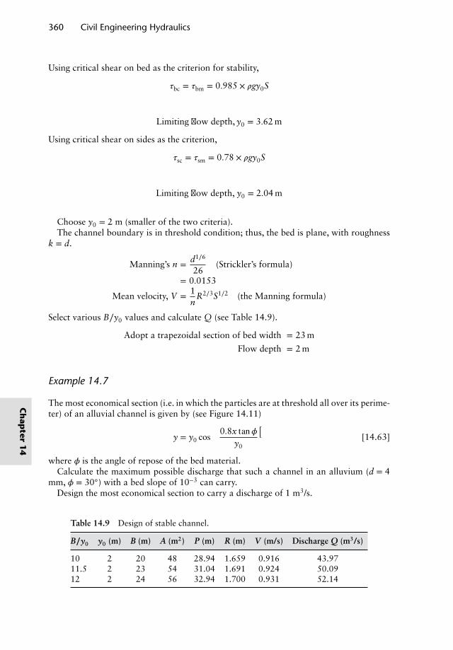
360 Civil Engineering Hydraulics
Using critical shear on bed as the criterion for stability,
𝜏bc = 𝜏bm = 0.985 × 𝜌gy0S
Limiting flow depth, y0 = 3.62 m
Using critical shear on sides as the criterion,
𝜏sc = 𝜏sm = 0.78 × 𝜌gy0S
Limiting flow depth, y0 = 2.04 m
Choose y0 = 2 m (smaller of the two criteria).The channel boundary is in threshold condition; thus, the bed is plane, with roughness
k = d.
Manning’s n = d1∕6
26(Strickler’s formula)
= 0.0153
Mean velocity, V = 1n
R2∕3S1∕2 (the Manning formula)
Select various B∕y0 values and calculate Q (see Table 14.9).
Adopt a trapezoidal section of bed width = 23 m
Flow depth = 2 m
Example 14.7
The most economical section (i.e. in which the particles are at threshold all over its perime-ter) of an alluvial channel is given by (see Figure 14.11)
y = y0 cos(
0.8x tan𝜙y0
)[14.63]
where 𝜙 is the angle of repose of the bed material.Calculate the maximum possible discharge that such a channel in an alluvium (d = 4
mm, 𝜙 = 30◦) with a bed slope of 10−3 can carry.Design the most economical section to carry a discharge of 1 m3/s.
Table 14.9 Design of stable channel.
B∕y0 y0 (m) B (m) A (m2) P (m) R (m) V (m/s) Discharge Q (m3/s)
10 2 20 48 28.94 1.659 0.916 43.9711.5 2 23 54 31.04 1.691 0.924 50.0912 2 24 56 32.94 1.700 0.931 52.14
Ch
apter
14
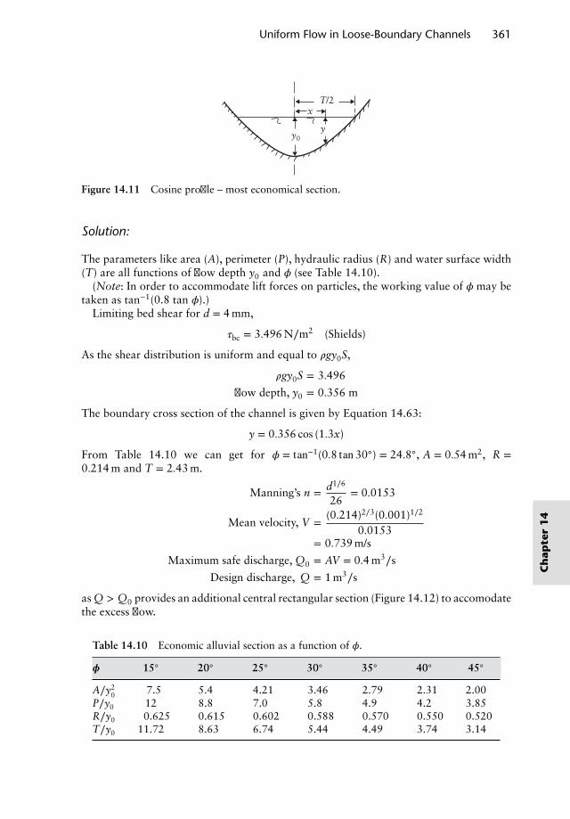
Uniform Flow in Loose-Boundary Channels 361
x
yy0
T/2
Figure 14.11 Cosine profile – most economical section.
Solution:
The parameters like area (A), perimeter (P), hydraulic radius (R) and water surface width(T) are all functions of flow depth y0 and 𝜙 (see Table 14.10).
(Note: In order to accommodate lift forces on particles, the working value of 𝜙 may betaken as tan−1(0.8 tan 𝜙).)
Limiting bed shear for d = 4 mm,
𝜏bc = 3.496 N∕m2 (Shields)
As the shear distribution is uniform and equal to 𝜌gy0S,
𝜌gy0S = 3.496
flow depth, y0 = 0.356 m
The boundary cross section of the channel is given by Equation 14.63:
y = 0.356 cos (1.3x)
From Table 14.10 we can get for 𝜙 = tan−1(0.8 tan 30◦) = 24.8◦, A = 0.54 m2, R =0.214 m and T = 2.43 m.
Manning’s n = d1∕6
26= 0.0153
Mean velocity, V = (0.214)2∕3(0.001)1∕2
0.0153= 0.739 m/s
Maximum safe discharge, Q0 = AV = 0.4 m3∕s
Design discharge, Q = 1 m3∕s
as Q > Q0 provides an additional central rectangular section (Figure 14.12) to accomodatethe excess flow.
Table 14.10 Economic alluvial section as a function of 𝜙.
𝝓 15◦ 20◦ 25◦ 30◦ 35◦ 40◦ 45◦
A∕y20 7.5 5.4 4.21 3.46 2.79 2.31 2.00
P∕y0 12 8.8 7.0 5.8 4.9 4.2 3.85R∕y0 0.625 0.615 0.602 0.588 0.570 0.550 0.520T∕y0 11.72 8.63 6.74 5.44 4.49 3.74 3.14
Ch
apte
r1
4
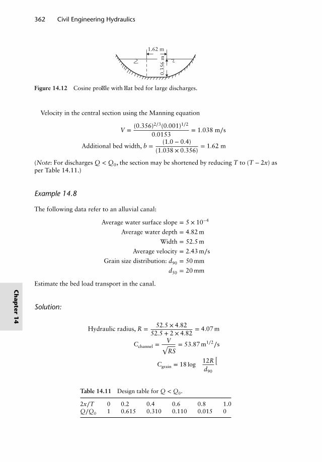
362 Civil Engineering Hydraulics
1.62 m
0.35
6 m
Figure 14.12 Cosine profile with flat bed for large discharges.
Velocity in the central section using the Manning equation
V =(0.356)2∕3(0.001)1∕2
0.0153= 1.038 m∕s
Additional bed width, b =(1.0 − 0.4)
(1.038 × 0.356)= 1.62 m
(Note: For discharges Q < Q0, the section may be shortened by reducing T to (T − 2x) asper Table 14.11.)
Example 14.8
The following data refer to an alluvial canal:
Average water surface slope = 5 × 10⁻⁴
Average water depth = 4.82 m
Width = 52.5 m
Average velocity = 2.43 m∕s
Grain size distribution: d90 = 50 mm
d50 = 20 mm
Estimate the bed load transport in the canal.
Solution:
Hydraulic radius, R = 52.5 × 4.8252.5 + 2 × 4.82
= 4.07 m
Cchannel =V√RS
= 53.87 m1∕2∕s
Cgrain = 18 log(
12Rd90
)
Table 14.11 Design table for Q < Q0.
2x∕T 0 0.2 0.4 0.6 0.8 1.0Q∕Q0 1 0.615 0.310 0.110 0.015 0
Ch
apter
14
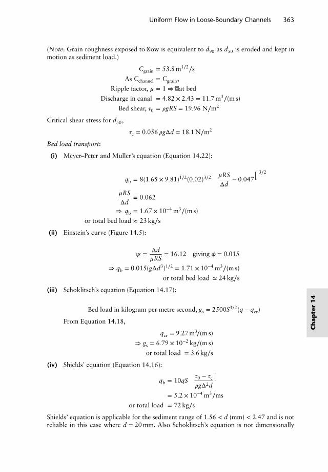
Uniform Flow in Loose-Boundary Channels 363
(Note: Grain roughness exposed to flow is equivalent to d90 as d50 is eroded and kept inmotion as sediment load.)
Cgrain = 53.8 m1∕2∕s
As Cchannel = Cgrain,
Ripple factor, 𝜇 = 1 ⇒ flat bed
Discharge in canal = 4.82 × 2.43 = 11.7 m3∕(m s)
Bed shear, 𝜏0 = 𝜌gRS = 19.96 N∕m2
Critical shear stress for d50,
𝜏c = 0.056 𝜌gΔd = 18.1 N∕m2
Bed load transport:
(i) Meyer–Peter and Muller’s equation (Equation 14.22):
qb = 8(1.65 × 9.81)1∕2(0.02)3∕2(𝜇RSΔd
− 0.047)3∕2
𝜇RSΔd
= 0.062
⇒ qb = 1.67 × 10⁻⁴ m3∕(m s)
or total bed load ≈ 23 kg∕s
(ii) Einstein’s curve (Figure 14.5):
𝜓 = Δd𝜇RS
= 16.12 giving 𝜙 = 0.015
⇒ qb = 0.015(gΔd3)1∕2 = 1.71 × 10⁻⁴ m3∕(m s)
or total bed load ≃ 24 kg∕s
(iii) Schoklitsch’s equation (Equation 14.17):
Bed load in kilogram per metre second, gs = 2500S3∕2(q − qcr)
From Equation 14.18,
qcr = 9.27 m3∕(m s)
⇒ gs = 6.79 × 10⁻² kg∕(m s)
or total load = 3.6 kg∕s
(iv) Shields’ equation (Equation 14.16):
qb = 10qS(𝜏0 − 𝜏c
𝜌gΔ2d
)= 5.2 × 10⁻⁴ m3∕ms
or total load = 72 kg∕s
Shields’ equation is applicable for the sediment range of 1.56 < d (mm) < 2.47 and is notreliable in this case where d = 20 mm. Also Schoklitsch’s equation is not dimensionally
Ch
apte
r1
4
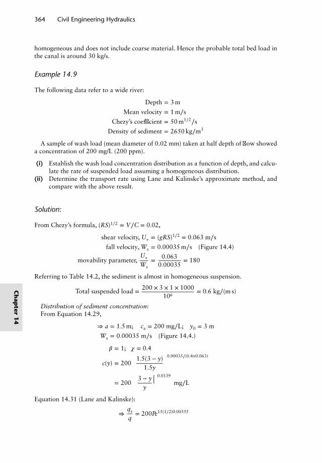
364 Civil Engineering Hydraulics
homogeneous and does not include coarse material. Hence the probable total bed load inthe canal is around 30 kg/s.
Example 14.9
The following data refer to a wide river:
Depth = 3 m
Mean velocity = 1 m∕s
Chezy’s coefficient = 50 m1∕2∕s
Density of sediment = 2650 kg∕m3
A sample of wash load (mean diameter of 0.02 mm) taken at half depth of flow showeda concentration of 200 mg/L (200 ppm).
(i) Establish the wash load concentration distribution as a function of depth, and calcu-late the rate of suspended load assuming a homogeneous distribution.
(ii) Determine the transport rate using Lane and Kalinske’s approximate method, andcompare with the above result.
Solution:
From Chezy’s formula, (RS)1∕2 = V∕C = 0.02,
shear velocity, U∗ = (gRS)1∕2 = 0.063 m∕s
fall velocity, Ws = 0.00035 m∕s (Figure 14.4)
movability parameter,U∗
Ws= 0.063
0.00035= 180
Referring to Table 14.2, the sediment is almost in homogeneous suspension.
Total suspended load = 200 × 3 × 1 × 1000106
= 0.6 kg∕(m s)
Distribution of sediment concentration:From Equation 14.29,
⇒ a = 1.5 m; ca = 200 mg∕L; y0 = 3 m
Ws = 0.00035 m∕s (Figure 14.4.)
𝛽 = 1; 𝜒 = 0.4
c(y) = 200[
1.5(3 − y)1.5y
]0.00035∕(0.4×0.063)
= 200(
3 − yy
)0.0139
mg∕L
Equation 14.31 (Lane and Kalinske):
⇒qs
q= 200Pe15(1∕2)0.00555
Ch
apter
14
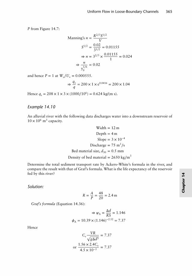
Uniform Flow in Loose-Boundary Channels 365
P from Figure 14.7:
Manning’s n = R2∕3S1∕2
V
S1∕2 = 0.0231∕2
= 0.01155
⇒ n = 32∕3 × 0.011551
= 0.024
⇒n
y1∕60
= 0.02
and hence P = 1 at Ws∕U∗ = 0.000555.
⇒qs
q= 200 × 1 × e0.0416 = 200 × 1.04
Hence qs = 208 × 1 × 3 × (1000∕106) = 0.624 kg/(m s).
Example 14.10
An alluvial river with the following data discharges water into a downstream reservoir of10 × 106 m3 capacity.
Width = 12 m
Depth = 4 m
Slope = 3 × 10⁻⁴
Discharge = 75 m3∕s
Bed material size, d50 = 0.5 mm
Density of bed material = 2650 kg∕m3
Determine the total sediment transport rate by Ackers–White’s formula in the river, andcompare the result with that of Graf’s formula. What is the life expectancy of the reservoirfed by this river?
Solution:
R = AP
= 4820
= 2.4 m
Graf’s formula (Equation 14.36):
⇒ 𝜓A = ΔdRS
= 1.146
𝜙A = 10.39 × (1.146)−2.52 = 7.37
Hence
CvVR√gΔd3
= 7.37
or1.56 × 2.4Cv
4.5 × 10−5= 7.37
Ch
apte
r1
4
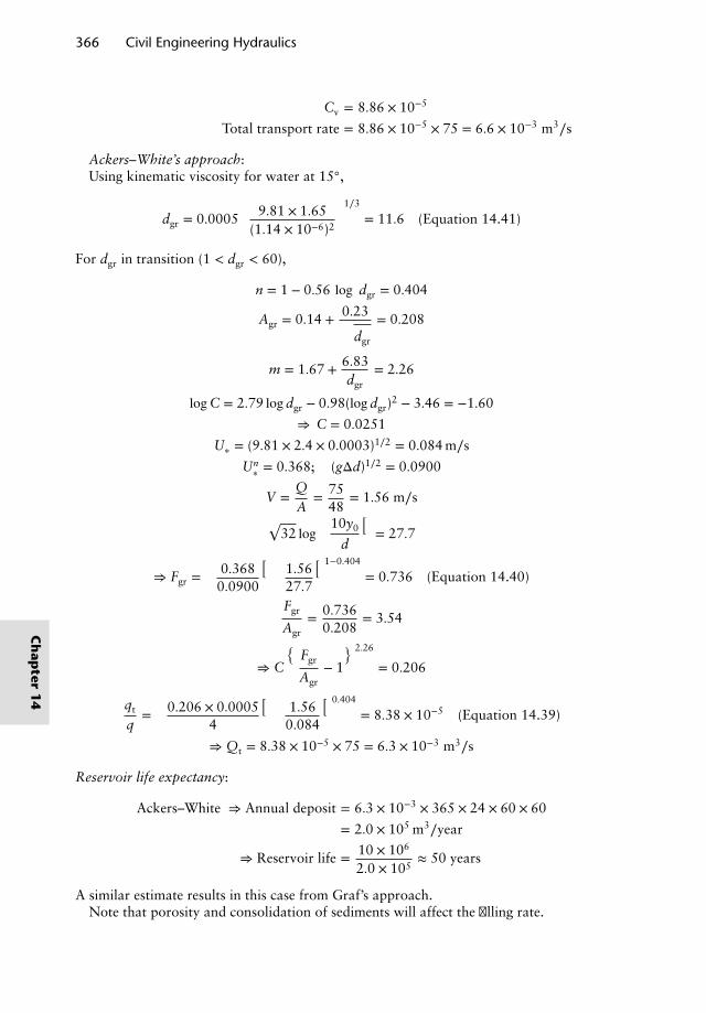
366 Civil Engineering Hydraulics
Cv = 8.86 × 10⁻⁵
Total transport rate = 8.86 × 10−5 × 75 = 6.6 × 10⁻³ m3∕s
Ackers–White’s approach:Using kinematic viscosity for water at 15◦,
dgr = 0.0005[
9.81 × 1.65(1.14 × 10⁻⁶)2
]1∕3
= 11.6 (Equation 14.41)
For dgr in transition (1 < dgr < 60),
n = 1 − 0.56 log dgr = 0.404
Agr = 0.14 + 0.23√dgr
= 0.208
m = 1.67 + 6.83dgr
= 2.26
logC = 2.79 logdgr − 0.98(logdgr)2 − 3.46 = −1.60
⇒ C = 0.0251
U∗ = (9.81 × 2.4 × 0.0003)1∕2 = 0.084 m∕s
Un∗ = 0.368; (gΔd)1∕2 = 0.0900
V =QA
= 7548
= 1.56 m∕s
√32 log
(10y0
d
)= 27.7
⇒ Fgr =(
0.3680.0900
)(1.5627.7
)1−0.404
= 0.736 (Equation 14.40)
Fgr
Agr= 0.736
0.208= 3.54
⇒ C
(Fgr
Agr− 1
)2.26
= 0.206
qt
q=(
0.206 × 0.00054
)(1.560.084
)0.404
= 8.38 × 10⁻⁵ (Equation 14.39)
⇒ Qt = 8.38 × 10−5 × 75 = 6.3 × 10⁻³ m3∕s
Reservoir life expectancy:
Ackers–White ⇒ Annual deposit = 6.3 × 10−3 × 365 × 24 × 60 × 60
= 2.0 × 10⁵ m3∕year
⇒ Reservoir life = 10 × 106
2.0 × 10⁵≈ 50 years
A similar estimate results in this case from Graf’s approach.Note that porosity and consolidation of sediments will affect the filling rate.
Ch
apter
14
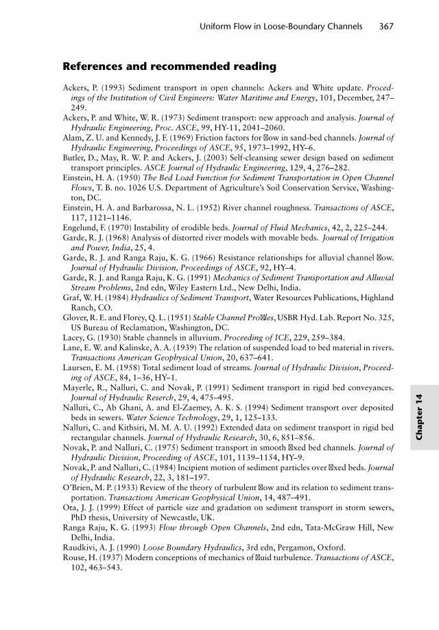
Uniform Flow in Loose-Boundary Channels 367
References and recommended reading
Ackers, P. (1993) Sediment transport in open channels: Ackers and White update. Proced-ings of the Institution of Civil Engineers: Water Maritime and Energy, 101, December, 247–249.
Ackers, P. and White, W. R. (1973) Sediment transport: new approach and analysis. Journal ofHydraulic Engineering, Proc. ASCE, 99, HY-11, 2041–2060.
Alam, Z. U. and Kennedy, J. F. (1969) Friction factors for flow in sand-bed channels. Journal ofHydraulic Engineering, Proceedings of ASCE, 95, 1973–1992, HY–6.
Butler, D., May, R. W. P. and Ackers, J. (2003) Self-cleansing sewer design based on sedimenttransport principles. ASCE Journal of Hydraulic Engineering, 129, 4, 276–282.
Einstein, H. A. (1950) The Bed Load Function for Sediment Transportation in Open ChannelFlows, T. B. no. 1026 U.S. Department of Agriculture’s Soil Conservation Service, Washing-ton, DC.
Einstein, H. A. and Barbarossa, N. L. (1952) River channel roughness. Transactions of ASCE,117, 1121–1146.
Engelund, F. (1970) Instability of erodible beds. Journal of Fluid Mechanics, 42, 2, 225–244.Garde, R. J. (1968) Analysis of distorted river models with movable beds. Journal of Irrigation
and Power, India, 25, 4.Garde, R. J. and Ranga Raju, K. G. (1966) Resistance relationships for alluvial channel flow.
Journal of Hydraulic Division, Proceedings of ASCE, 92, HY–4.Garde, R. J. and Ranga Raju, K. G. (1991) Mechanics of Sediment Transportation and Alluvial
Stream Problems, 2nd edn, Wiley Eastern Ltd., New Delhi, India.Graf, W. H. (1984) Hydraulics of Sediment Transport, Water Resources Publications, Highland
Ranch, CO.Glover, R. E. and Florey, Q. L. (1951) Stable Channel Profiles, USBR Hyd. Lab. Report No. 325,
US Bureau of Reclamation, Washington, DC.Lacey, G. (1930) Stable channels in alluvium. Proceeding of ICE, 229, 259–384.Lane, E. W. and Kalinske, A. A. (1939) The relation of suspended load to bed material in rivers.
Transactions American Geophysical Union, 20, 637–641.Laursen, E. M. (1958) Total sediment load of streams. Journal of Hydraulic Division, Proceed-
ing of ASCE, 84, 1–36, HY–1.Mayerle, R., Nalluri, C. and Novak, P. (1991) Sediment transport in rigid bed conveyances.
Journal of Hydraulic Reserch, 29, 4, 475–495.Nalluri, C., Ab Ghani, A. and El-Zaemey, A. K. S. (1994) Sediment transport over deposited
beds in sewers. Water Science Technology, 29, 1, 125–133.Nalluri, C. and Kithsiri, M. M. A. U. (1992) Extended data on sediment transport in rigid bed
rectangular channels. Journal of Hydraulic Research, 30, 6, 851–856.Novak, P. and Nalluri, C. (1975) Sediment transport in smooth fixed bed channels. Journal of
Hydraulic Division, Proceeding of ASCE, 101, 1139–1154, HY–9.Novak, P. and Nalluri, C. (1984) Incipient motion of sediment particles over fixed beds. Journal
of Hydraulic Research, 22, 3, 181–197.O’Brien, M. P. (1933) Review of the theory of turbulent flow and its relation to sediment trans-
portation. Transactions American Geophysical Union, 14, 487–491.Ota, J. J. (1999) Effect of particle size and gradation on sediment transport in storm sewers,
PhD thesis, University of Newcastle, UK.Ranga Raju, K. G. (1993) Flow through Open Channels, 2nd edn, Tata-McGraw Hill, New
Delhi, India.Raudkivi, A. J. (1990) Loose Boundary Hydraulics, 3rd edn, Pergamon, Oxford.Rouse, H. (1937) Modern conceptions of mechanics of fluid turbulence. Transactions of ASCE,
102, 463–543.
Ch
apte
r1
4
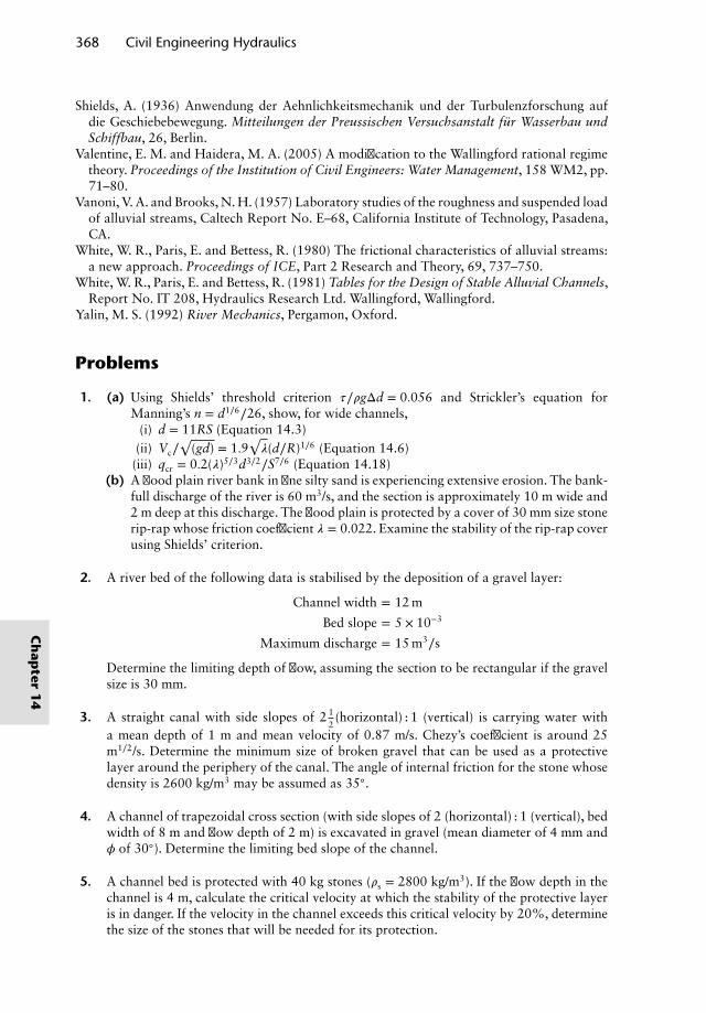
368 Civil Engineering Hydraulics
Shields, A. (1936) Anwendung der Aehnlichkeitsmechanik und der Turbulenzforschung aufdie Geschiebebewegung. Mitteilungen der Preussischen Versuchsanstalt fur Wasserbau undSchiffbau, 26, Berlin.
Valentine, E. M. and Haidera, M. A. (2005) A modification to the Wallingford rational regimetheory. Proceedings of the Institution of Civil Engineers: Water Management, 158 WM2, pp.71–80.
Vanoni, V. A. and Brooks, N. H. (1957) Laboratory studies of the roughness and suspended loadof alluvial streams, Caltech Report No. E–68, California Institute of Technology, Pasadena,CA.
White, W. R., Paris, E. and Bettess, R. (1980) The frictional characteristics of alluvial streams:a new approach. Proceedings of ICE, Part 2 Research and Theory, 69, 737–750.
White, W. R., Paris, E. and Bettess, R. (1981) Tables for the Design of Stable Alluvial Channels,Report No. IT 208, Hydraulics Research Ltd. Wallingford, Wallingford.
Yalin, M. S. (1992) River Mechanics, Pergamon, Oxford.
Problems
1. (a) Using Shields’ threshold criterion 𝜏∕𝜌gΔd = 0.056 and Strickler’s equation forManning’s n = d1∕6∕26, show, for wide channels,
(i) d = 11RS (Equation 14.3)(ii) Vc∕
√(gd) = 1.9
√𝜆(d∕R)1∕6 (Equation 14.6)
(iii) qcr = 0.2(𝜆)5∕3d3∕2∕S7∕6 (Equation 14.18)(b) A flood plain river bank in fine silty sand is experiencing extensive erosion. The bank-
full discharge of the river is 60 m3/s, and the section is approximately 10 m wide and2 m deep at this discharge. The flood plain is protected by a cover of 30 mm size stonerip-rap whose friction coefficient 𝜆 = 0.022. Examine the stability of the rip-rap coverusing Shields’ criterion.
2. A river bed of the following data is stabilised by the deposition of a gravel layer:
Channel width = 12 m
Bed slope = 5 × 10⁻³
Maximum discharge = 15 m3∕s
Determine the limiting depth of flow, assuming the section to be rectangular if the gravelsize is 30 mm.
3. A straight canal with side slopes of 2 12(horizontal) : 1 (vertical) is carrying water with
a mean depth of 1 m and mean velocity of 0.87 m/s. Chezy’s coefficient is around 25m1∕2/s. Determine the minimum size of broken gravel that can be used as a protectivelayer around the periphery of the canal. The angle of internal friction for the stone whosedensity is 2600 kg/m3 may be assumed as 35◦.
4. A channel of trapezoidal cross section (with side slopes of 2 (horizontal) : 1 (vertical), bedwidth of 8 m and flow depth of 2 m) is excavated in gravel (mean diameter of 4 mm and𝜙 of 30◦). Determine the limiting bed slope of the channel.
5. A channel bed is protected with 40 kg stones (𝜌s = 2800 kg/m3). If the flow depth in thechannel is 4 m, calculate the critical velocity at which the stability of the protective layeris in danger. If the velocity in the channel exceeds this critical velocity by 20%, determinethe size of the stones that will be needed for its protection.
Ch
apter
14
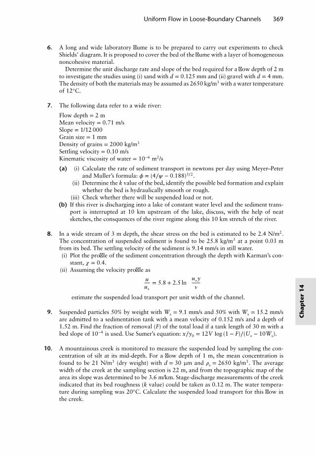
Uniform Flow in Loose-Boundary Channels 369
6. A long and wide laboratory flume is to be prepared to carry out experiments to checkShields’ diagram. It is proposed to cover the bed of the flume with a layer of homogeneousnoncohesive material.
Determine the unit discharge rate and slope of the bed required for a flow depth of 2 mto investigate the studies using (i) sand with d = 0.125 mm and (ii) gravel with d = 4 mm.The density of both the materials may be assumed as 2650 kg/m3 with a water temperatureof 12◦C.
7. The following data refer to a wide river:
Flow depth = 2 mMean velocity = 0.71 m/sSlope = 1/12 000Grain size = 1 mmDensity of grains = 2000 kg/m3
Settling velocity = 0.10 m/sKinematic viscosity of water = 10−6 m2/s
(a) (i) Calculate the rate of sediment transport in newtons per day using Meyer–Peterand Muller’s formula: 𝜙 = (4∕𝜓 − 0.188)3∕2.
(ii) Determine the k value of the bed, identify the possible bed formation and explainwhether the bed is hydraulically smooth or rough.
(iii) Check whether there will be suspended load or not.(b) If this river is discharging into a lake of constant water level and the sediment trans-
port is interrupted at 10 km upstream of the lake, discuss, with the help of neatsketches, the consquences of the river regime along this 10 km stretch of the river.
8. In a wide stream of 3 m depth, the shear stress on the bed is estimated to be 2.4 N/m2.
The concentration of suspended sediment is found to be 25.8 kg/m3 at a point 0.03 mfrom its bed. The settling velocity of the sediment is 9.14 mm/s in still water.(i) Plot the profile of the sediment concentration through the depth with Karman’s con-
stant, 𝜒 = 0.4.(ii) Assuming the velocity profile as
uu∗
= 5.8 + 2.5 ln(u∗y𝜈
)estimate the suspended load transport per unit width of the channel.
9. Suspended particles 50% by weight with Ws = 9.1 mm/s and 50% with Ws = 15.2 mm/sare admitted to a sedimentation tank with a mean velocity of 0.152 m/s and a depth of1.52 m. Find the fraction of removal (F) of the total load if a tank length of 30 m with abed slope of 10−4 is used. Use Sumer’s equation: x∕y0 = 12V log (1 − F)∕(U∗ − 10Ws).
10. A mountainous creek is monitored to measure the suspended load by sampling the con-centration of silt at its mid-depth. For a flow depth of 1 m, the mean concentration isfound to be 21 N/m3 (dry weight) with d = 30 μm and 𝜌s = 2650 kg/m3. The averagewidth of the creek at the sampling section is 22 m, and from the topographic map of thearea its slope was determined to be 3.6 m/km. Stage-discharge measurements of the creekindicated that its bed roughness (k value) could be taken as 0.12 m. The water tempera-ture during sampling was 20◦C. Calculate the suspended load transport for this flow inthe creek.
Ch
apte
r1
4

Chapter 15Hydraulic Structures
15.1 Introduction
A variety of hydraulic structures are available to control water levels and regulate dis-charges for purposes of water supply, water storage, flood alleviation, irrigation and soon. These range from the weirs/sluices of small channels to the overflow spillways oflarge dams. Many of these structures may also be used as discharge-measuring devices, asdescribed in standards such as BS3680 Part 4 (1981, 1990). This chapter mainly deals withthe spillways and their associated energy dissipators as examples of common hydraulicstructures.
15.2 Spillways
A spillway is the overflow device of a dam project which is essential to evacuate excessof water, which otherwise may cause upstream flooding, dam overtopping and eventuallydam failure. Basically there are three types of spillways: overfall (ogee or side channel),shaft (morning glory) and siphon. The overfall types are the most frequently encountered,and they are described here in detail. The reader may refer to Novak et al. (2007) for othertypes and further information.
15.2.1 Overfall spillways
The basic shape of the overfall spillway (ogee spillway) is derived from the lower envelopeof the overfall nappe (see Figure 15.1) flowing over a high vertical rectangular notch withan approaching velocity Va close to zero and a fully aerated space beneath the nappe (seealso Section 3.17.5). For a notch of width b, head h and discharge coefficient C′
d, the
Nalluri & Featherstone’s Civil Engineering Hydraulics: Essential Theory with Worked Examples,Sixth Edition. Martin Marriott.© 2016 John Wiley & Sons, Ltd. Published 2016 by John Wiley & Sons, Ltd.Companion Website: www.wiley.com/go/Marriott
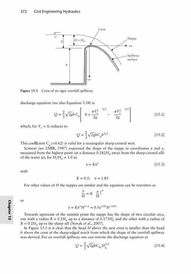
372 Civil Engineering Hydraulics
h
P
+y
+x
Spillwaysurface
Nappe
Crest
H = Hd
Figure 15.1 Crest of an ogee overfall spillway.
discharge equation (see also Equation 3.34) is
Q = 23
√2gb C′
d
⎡⎢⎢⎣(
h +𝛼V2
a
2g
)3∕2
−
(𝛼V2
a
2g
)3∕2⎤⎥⎥⎦ [15.1]
which, for Va = 0, reduces to
Q = 23
√2gbC′
dh3∕2 [15.2]
This coefficient C′d
(=0.62) is valid for a rectangular sharp-crested weir.Scimeni (see USBR, 1987) expressed the shape of the nappe in coordinates x and y,
measured from the highest point (at a distance 0.282Hd away from the sharp-crested sill)of the water jet, for H∕Hd = 1.0 as
y = Kxn [15.3]
with
K = 0.5; n = 1.85
For other values of H the nappes are similar and the equation can be rewritten as
yH
= K( x
H
)n
or
y = KxnH1−n = 0.5x1.85H−0.85
Towards upstream of the summit point the nappe has the shape of two circular arcs,one with a radius R = 0.5Hd up to a distance of 0.175Hd and the other with a radius ofR = 0.2Hd up to the sharp sill (Novak et al., 2007).
In Figure 15.1 it is clear that the head H above the new crest is smaller than the headh above the crest of the sharp-edged notch from which the shape of the overfall spillwaywas derived. For an overfall spillway one can rewrite the discharge equation as
Q = 23
√2gbCd0
H3∕2de
[15.4]
Ch
apter
15
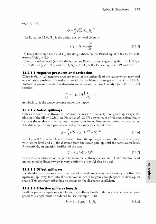
Hydraulic Structures 373
or, if Va = 0,
Q = 23
√2gbCd0
H3∕2d
In Equation 15.4, Hdeis the design energy head given by
Hde= Hd + 𝛼
V2a
2g[15.5]
Hd being the design head and Cd0the design discharge coefficient equal to 0.745 for spill-
ways of P∕Hde> 3.0.
For any other head (H) the discharge coefficient varies, suggesting that for H∕Hd <
1.0, 0.580 < Cd < 0.745, and for H∕Hd > 1.0, Cd > 0.745 (see Figures 3.19 and 3.20).
15.2.1.1 Negative pressures and cavitationWhen H∕Hd > 1.0, negative pressure exists on the underside of the nappe which may leadto cavitation problems. In order to avoid this problem it is suggested that H < 1.65Hd.To find the pressure under the downstream nappe one can use Cassidy’s (see USBR, 1987)relation:
pm
𝜌g= −1.17H
(HHd
− 1)
in which pm is the gauge pressure under the nappe.
15.2.1.2 Gated spillwaysGates are used in spillways to increase the reservoir capacity. For gated spillways, theplacing of the sill by 0.2Hd (see Novak et al., 2007) downstream of the crest substantiallyreduces the tendency towards negative pressures for outflow under partially raised gates.The discharge through partially raised gates can be calculated from
Q = 23
√2gbCd1
(H3∕2 − H3∕2
1
)[15.6]
with Cd1= 0.6, in which H is the distance from the spillway crest until the upstream (reser-
voir) water level and H1 the distance from the lower gate lip until the same water level.Alternatively, an equation (orifice) of the type
Q = Cd2ba(2gHe)
1∕2 [15.7]
where a is the distance of the gate lip from the spillway surface and He the effective headon the gated spillway (which is very similar to H) could also be used.
15.2.1.3 Offset spillwaysFor slender dam sections as in the case of arch dams, it may be necessary to offset theupstream spillway face into the reservoir in order to gain enough space to develop itsshape. This upstream offset has no effects on the discharge coefficient.
15.2.1.4 Effective spillway lengthIn all the previous equations, b refers to the spillway length. If the crest has piers (to supportgates) this length must be reduced to (see Example 3.18)
be = b − 2(nkp + ka)He [15.8]
Ch
apte
r1
5
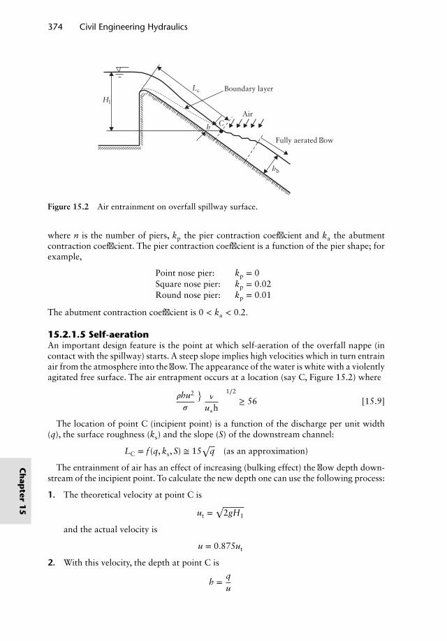
374 Civil Engineering Hydraulics
Boundary layer
Air
Fully aerated flow
hb
Lc
Hl
h C
Figure 15.2 Air entrainment on overfall spillway surface.
where n is the number of piers, kp the pier contraction coefficient and ka the abutmentcontraction coefficient. The pier contraction coefficient is a function of the pier shape; forexample,
Point nose pier: kp = 0Square nose pier: kp = 0.02Round nose pier: kp = 0.01
The abutment contraction coefficient is 0 < ka < 0.2.
15.2.1.5 Self-aerationAn important design feature is the point at which self-aeration of the overfall nappe (incontact with the spillway) starts. A steep slope implies high velocities which in turn entrainair from the atmosphere into the flow. The appearance of the water is white with a violentlyagitated free surface. The air entrapment occurs at a location (say C, Figure 15.2) where
𝜌hu2
𝜎
(𝜈
u∗h
)1∕2
≥ 56 [15.9]
The location of point C (incipient point) is a function of the discharge per unit width(q), the surface roughness (ks) and the slope (S) of the downstream channel:
LC = f (q, ks, S) ≅ 15√
q (as an approximation)
The entrainment of air has an effect of increasing (bulking effect) the flow depth down-stream of the incipient point. To calculate the new depth one can use the following process:
1. The theoretical velocity at point C is
ut =√
2gH1
and the actual velocity is
u = 0.875ut
2. With this velocity, the depth at point C is
h =qu
Ch
apter
15
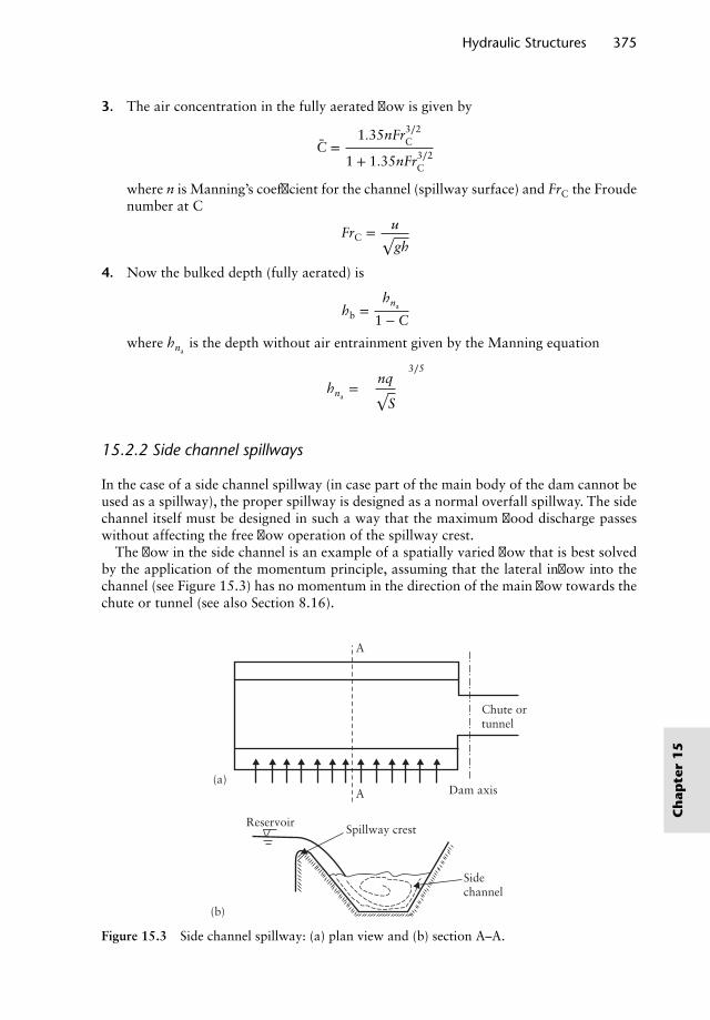
Hydraulic Structures 375
3. The air concentration in the fully aerated flow is given by
C =1.35nFr3∕2
C
1 + 1.35nFr3∕2C
where n is Manning’s coefficient for the channel (spillway surface) and FrC the Froudenumber at C
FrC = u√gh
4. Now the bulked depth (fully aerated) is
hb =hna
1 − C
where hnais the depth without air entrainment given by the Manning equation
hna=
(nq√
S
)3∕5
15.2.2 Side channel spillways
In the case of a side channel spillway (in case part of the main body of the dam cannot beused as a spillway), the proper spillway is designed as a normal overfall spillway. The sidechannel itself must be designed in such a way that the maximum flood discharge passeswithout affecting the free flow operation of the spillway crest.
The flow in the side channel is an example of a spatially varied flow that is best solvedby the application of the momentum principle, assuming that the lateral inflow into thechannel (see Figure 15.3) has no momentum in the direction of the main flow towards thechute or tunnel (see also Section 8.16).
Chute ortunnel
A
A Dam axis
Spillway crestReservoir
Sidechannel
(a)
(b)
Figure 15.3 Side channel spillway: (a) plan view and (b) section A–A.
Ch
apte
r1
5
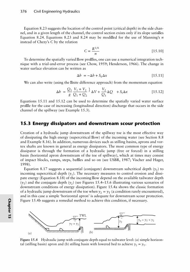
376 Civil Engineering Hydraulics
Equation 8.23 suggests the location of the control point (critical depth) in the side chan-nel, and in a given length of the channel, the control section exists only if its slope satisfiesEquation 8.24. Equations 8.23 and 8.24 may be modified for the use of Manning’s ninstead of Chezy’s C by the relation
C = R1∕6
n[15.10]
To determine the spatially varied flow profiles, one can use a numerical integration tech-nique with a trial-and-error process (see Chow, 1959; Henderson, 1966). The change inwater surface elevation can be written as
Δh′ = −Δh + S0Δx [15.11]
We can also write (using the finite difference approach) from the momentum equation
Δh′ =Q1
gV1 + V2
Q1 + Q2
(ΔV +
V2
Q1ΔQ
)+ SfΔx [15.12]
Equations 15.11 and 15.12 can be used to determine the spatially varied water surfaceprofile for the case of increasing (longitudinal direction) discharge that occurs in the sidechannel of the spillway (see Example 15.3).
15.3 Energy dissipators and downstream scour protection
Creation of a hydraulic jump downstream of the spillway toe is the most effective wayof dissipating the high energy (supercritical flow) of the incoming water (see Section 8.8and Example 8.16). In addition, numerous devices such as stilling basins, aprons and vor-tex shafts are known in general as energy dissipators. The most common type of energydissipator is through the formation of a hydraulic jump (free or forced) in a stillingbasin (horizontal apron downstream of the toe of spillway), which at times may consistof impact blocks, ramps, steps, baffles and so on (see USBR, 1987; Vischer and Hager,1998).
Equation 8.17 suggests a sequential (conjugate) downstream subcritical depth (y2) toincoming supercritical depth (y1). The necessary measures to control erosion and dissi-pate energy (Equation 8.18) of the incoming flow depend on the available tailwater depth(yT) and the conjugate depth (y2) (see Figures 15.4–15.6 illustrating various scenarios ofdownstream conditions of energy dissipation). Figure 15.4a shows the classic formationof a hydraulic jump downstream of the toe when y2 = yT (a condition rarely encountered),and in this case a simple ‘horizontal apron’ is adequate for downstream scour protection.Figure 15.4b suggests a remedial method to achieve this condition, if necessary.
TWL
(a) (b)
yT = y2
yn = yT < y2y2
Figure 15.4 Hydraulic jump with conjugate depth equal to tailwater level: (a) simple horizon-tal (stilling basin) apron and (b) stilling basin with lowered bed to achieve y2 = yT.
Ch
apter
15
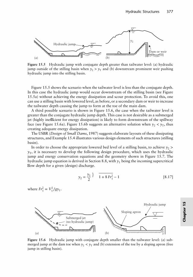
Hydraulic Structures 377
y2Hydraulic jump
(a) (b)
Dam or weir
Figure 15.5 Hydraulic jump with conjugate depth greater than tailwater level: (a) hydraulicjump outside of the stilling basin when y2 > yT and (b) downstream prominent weir pushinghydraulic jump into the stilling basin.
Figure 15.5 shows the scenario when the tailwater level is less than the conjugate depth.In this case the hydraulic jump would occur downstream of the stilling basin (see Figure15.5a) without achieving the energy dissipation and scour protection. To avoid this, onecan use a stilling basin with lowered level, as before, or a secondary dam or weir to increasethe tailwater depth causing the jump to form at the toe of the main dam.
A third possible scenario is shown in Figure 15.6, the case when the tailwater level isgreater than the conjugate hydraulic jump depth. This case is not desirable as a submergedjet (highly inefficient for energy dissipation) is likely to form downstream of the spillwayface (see Figure 15.6a). Figure 15.6b suggests an alternative solution when y2 < yT, thuscreating adequate energy dissipation.
The USBR (Design of Small Dams, 1987) suggests elaborate layouts of these dissipatingstructures, and Example 15.4 illustrates various design elements of such structures (stillingbasin).
In order to choose the appropriate lowered bed level of a stilling basin, to achieve y2 >
yT, it is necessary to develop the following design procedure, which uses the hydraulicjump and energy conservation equations and the geometry shown in Figure 15.7. Thehydraulic jump equation is derived in Section 8.8, with y1 being the incoming supercriticalflow depth for a given (design) discharge.
y2 =y1
2
(√1 + 8 Fr2
1 − 1)
[8.17]
where Fr21 = V2
1∕gy1.
Submerged jet(no hydraulic jump)
Sloping apron
Hydraulic jump
(b)(a)
Figure 15.6 Hydraulic jump with conjugate depth smaller than the tailwater level: (a) sub-merged jump at the dam toe when y2 < yT and (b) extension of the toe by a sloping apron (freejump in stilling basin).
Ch
apte
r1
5
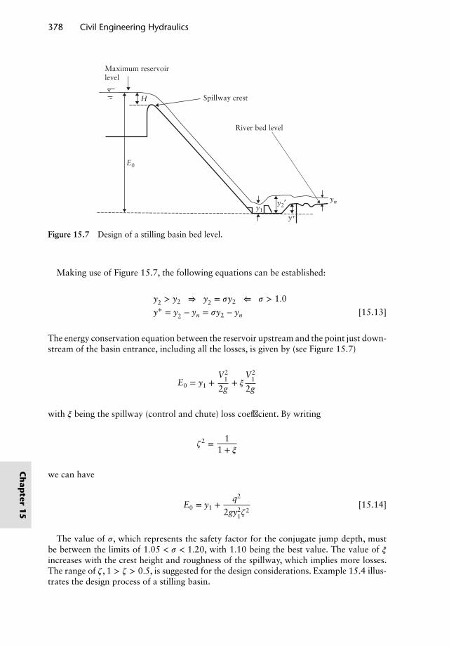
378 Civil Engineering Hydraulics
E0
y1y2′ yn
y+
H Spillway crest
River bed level
Maximum reservoirlevel
Figure 15.7 Design of a stilling basin bed level.
Making use of Figure 15.7, the following equations can be established:
y′2 > y2 ⇒ y′2 = 𝜎y2 ⇐ 𝜎 > 1.0
y+ = y′2 − yn = 𝜎y2 − yn [15.13]
The energy conservation equation between the reservoir upstream and the point just down-stream of the basin entrance, including all the losses, is given by (see Figure 15.7)
E0 = y1 +V2
1
2g+ 𝜉
V21
2g
with 𝜉 being the spillway (control and chute) loss coefficient. By writing
𝜁2 = 11 + 𝜉
we can have
E0 = y1 +q2
2gy21𝜁
2[15.14]
The value of 𝜎, which represents the safety factor for the conjugate jump depth, mustbe between the limits of 1.05 < 𝜎 < 1.20, with 1.10 being the best value. The value of 𝜉increases with the crest height and roughness of the spillway, which implies more losses.The range of 𝜁 , 1 > 𝜁 > 0.5, is suggested for the design considerations. Example 15.4 illus-trates the design process of a stilling basin.
Ch
apter
15
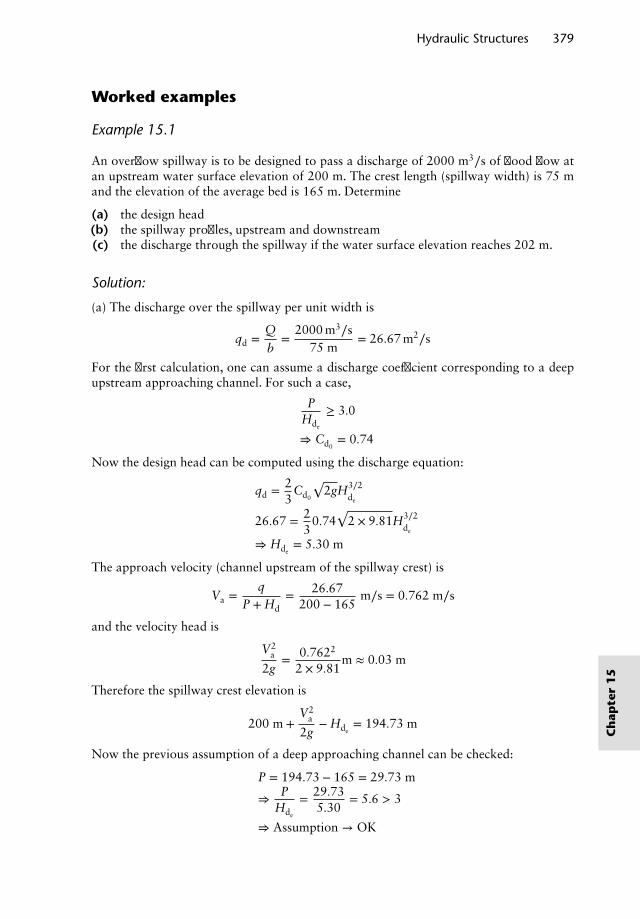
Hydraulic Structures 379
Worked examples
Example 15.1
An overflow spillway is to be designed to pass a discharge of 2000 m3∕s of flood flow atan upstream water surface elevation of 200 m. The crest length (spillway width) is 75 mand the elevation of the average bed is 165 m. Determine
(a) the design head(b) the spillway profiles, upstream and downstream(c) the discharge through the spillway if the water surface elevation reaches 202 m.
Solution:
(a) The discharge over the spillway per unit width is
qd =Q
b=
2000 m3∕s75 m
= 26.67 m2∕s
For the first calculation, one can assume a discharge coefficient corresponding to a deepupstream approaching channel. For such a case,
PHde
≥ 3.0
⇒ Cd0= 0.74
Now the design head can be computed using the discharge equation:
qd = 23
Cd0
√2gH3∕2
de
26.67 = 23
0.74√
2 × 9.81H3∕2de
⇒ Hde= 5.30 m
The approach velocity (channel upstream of the spillway crest) is
Va =q
P + Hd= 26.67
200 − 165m∕s = 0.762 m∕s
and the velocity head is
V2a
2g= 0.7622
2 × 9.81m ≈ 0.03 m
Therefore the spillway crest elevation is
200 m +V2
a
2g− Hde
= 194.73 m
Now the previous assumption of a deep approaching channel can be checked:
P = 194.73 − 165 = 29.73 m
⇒P
Hde
= 29.735.30
= 5.6 > 3
⇒ Assumption → OK
Ch
apte
r1
5
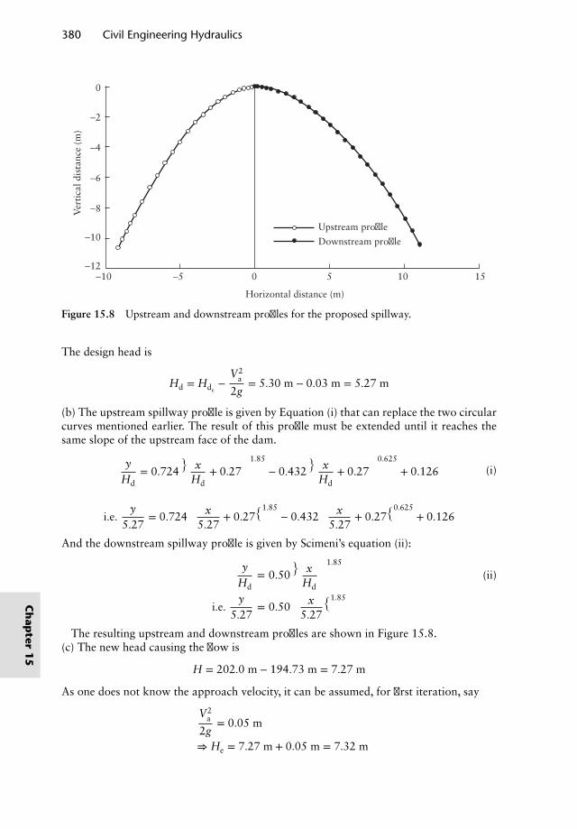
380 Civil Engineering Hydraulics
Upstream profile
Downstream profile
−10
0
−2
−4
−6
−8
−10
−12−5 0
Horizontal distance (m)
Ver
tica
l dis
tanc
e (m
)
5 10 15
Figure 15.8 Upstream and downstream profiles for the proposed spillway.
The design head is
Hd = Hde−
V2a
2g= 5.30 m − 0.03 m = 5.27 m
(b) The upstream spillway profile is given by Equation (i) that can replace the two circularcurves mentioned earlier. The result of this profile must be extended until it reaches thesame slope of the upstream face of the dam.
yHd
= 0.724(
xHd
+ 0.27)1.85
− 0.432(
xHd
+ 0.27)0.625
+ 0.126 (i)
i.e.y
5.27= 0.724
( x5.27
+ 0.27)1.85
− 0.432( x
5.27+ 0.27
)0.625+ 0.126
And the downstream spillway profile is given by Scimeni’s equation (ii):
yHd
= 0.50(
xHd
)1.85
(ii)
i.e.y
5.27= 0.50
( x5.27
)1.85
The resulting upstream and downstream profiles are shown in Figure 15.8.(c) The new head causing the flow is
H = 202.0 m − 194.73 m = 7.27 m
As one does not know the approach velocity, it can be assumed, for first iteration, say
V2a
2g= 0.05 m
⇒ He = 7.27 m + 0.05 m = 7.32 m
Ch
apter
15
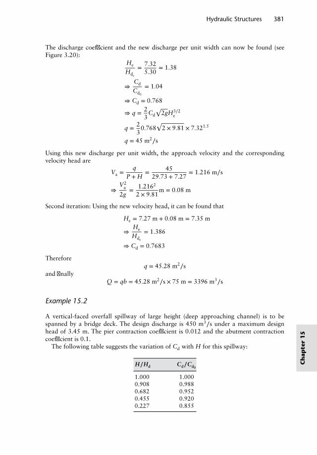
Hydraulic Structures 381
The discharge coefficient and the new discharge per unit width can now be found (seeFigure 3.20):
He
Hde
= 7.325.30
= 1.38
⇒Cd
Cd0
= 1.04
⇒ Cd = 0.768
⇒ q = 23
Cd
√2gH3∕2
e
q = 23
0.768√
2 × 9.81 × 7.321.5
q = 45 m2∕s
Using this new discharge per unit width, the approach velocity and the correspondingvelocity head are
Va =q
P + H= 45
29.73 + 7.27= 1.216 m∕s
⇒V2
a
2g= 1.2162
2 × 9.81m = 0.08 m
Second iteration: Using the new velocity head, it can be found that
He = 7.27 m + 0.08 m = 7.35 m
⇒He
Hde
= 1.386
⇒ Cd = 0.7683
Thereforeq = 45.28 m2∕s
and finallyQ = qb = 45.28 m2∕s × 75 m = 3396 m3∕s
Example 15.2
A vertical-faced overfall spillway of large height (deep approaching channel) is to bespanned by a bridge deck. The design discharge is 450 m3∕s under a maximum designhead of 3.45 m. The pier contraction coefficient is 0.012 and the abutment contractioncoefficient is 0.1.
The following table suggests the variation of Cd with H for this spillway:
H∕Hd Cd∕Cd0
1.000 1.0000.908 0.9880.682 0.9520.455 0.9200.227 0.855
Ch
apte
r1
5
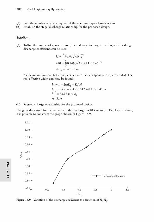
382 Civil Engineering Hydraulics
(a) Find the number of spans required if the maximum span length is 7 m.(b) Establish the stage–discharge relationship for the proposed design.
Solution:
(a) To find the number of spans required, the spillway discharge equation, with the designdischarge coefficient, can be used:
Q = 23
Cd0be
√2gH3∕2
d
450 = 23
0.74be
√2 × 9.81 × 3.453∕2
⇒ be = 32.136 m
As the maximum span between piers is 7 m, 4 piers (5 spans of 7 m) are needed. Thereal effective width can now be found:
be = b − 2(nKp + Ka)H
beR= 35 m − 2(4 × 0.012 + 0.1) × 3.45 m
beR= 33.98 m > be
⇒ Safe
(b) Stage–discharge relationship for the proposed design.
Using the data given for the variation of the discharge coefficient and an Excel spreadsheet,it is possible to construct the graph shown in Figure 15.9.
Ratio of coefficients
1.2
1.02
1.00
0.98
0.96
0.94
0.92
0.90
0.88
0.86
0.8410.80.60.40.20
H/Hd
C/C
d
Figure 15.9 Variation of the discharge coefficient as a function of H∕Hd.
Ch
apter
15
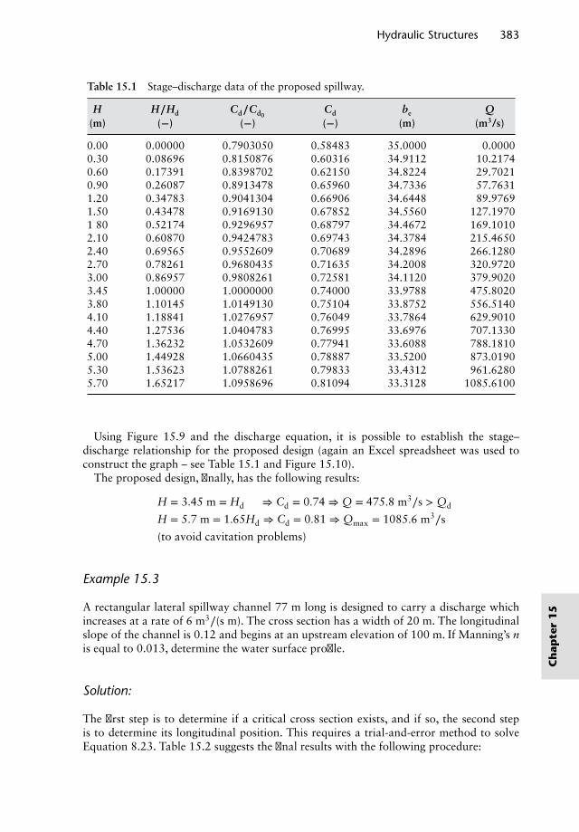
Hydraulic Structures 383
Table 15.1 Stage–discharge data of the proposed spillway.
H H∕Hd Cd∕Cd0Cd be Q
(m) (−) (−) (−) (m) (m3/s)
0.00 0.00000 0.7903050 0.58483 35.0000 0.00000.30 0.08696 0.8150876 0.60316 34.9112 10.21740.60 0.17391 0.8398702 0.62150 34.8224 29.70210.90 0.26087 0.8913478 0.65960 34.7336 57.76311.20 0.34783 0.9041304 0.66906 34.6448 89.97691.50 0.43478 0.9169130 0.67852 34.5560 127.19701 80 0.52174 0.9296957 0.68797 34.4672 169.10102.10 0.60870 0.9424783 0.69743 34.3784 215.46502.40 0.69565 0.9552609 0.70689 34.2896 266.12802.70 0.78261 0.9680435 0.71635 34.2008 320.97203.00 0.86957 0.9808261 0.72581 34.1120 379.90203.45 1.00000 1.0000000 0.74000 33.9788 475.80203.80 1.10145 1.0149130 0.75104 33.8752 556.51404.10 1.18841 1.0276957 0.76049 33.7864 629.90104.40 1.27536 1.0404783 0.76995 33.6976 707.13304.70 1.36232 1.0532609 0.77941 33.6088 788.18105.00 1.44928 1.0660435 0.78887 33.5200 873.01905.30 1.53623 1.0788261 0.79833 33.4312 961.62805.70 1.65217 1.0958696 0.81094 33.3128 1085.6100
Using Figure 15.9 and the discharge equation, it is possible to establish the stage–discharge relationship for the proposed design (again an Excel spreadsheet was used toconstruct the graph – see Table 15.1 and Figure 15.10).
The proposed design, finally, has the following results:
H = 3.45 m = Hd ⇒ Cd = 0.74 ⇒ Q = 475.8 m3∕s > Qd
H = 5.7 m = 1.65Hd ⇒ Cd = 0.81 ⇒ Qmax = 1085.6 m3∕s
(to avoid cavitation problems)
Example 15.3
A rectangular lateral spillway channel 77 m long is designed to carry a discharge whichincreases at a rate of 6 m3∕(s m). The cross section has a width of 20 m. The longitudinalslope of the channel is 0.12 and begins at an upstream elevation of 100 m. If Manning’s nis equal to 0.013, determine the water surface profile.
Solution:
The first step is to determine if a critical cross section exists, and if so, the second stepis to determine its longitudinal position. This requires a trial-and-error method to solveEquation 8.23. Table 15.2 suggests the final results with the following procedure:
Ch
apte
r1
5
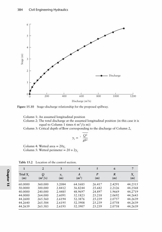
384 Civil Engineering Hydraulics
Discharge
Discharge (m3/s)
Stag
e (m
)
1200100080060040020000
1
2
3
4
5
6
Figure 15.10 Stage–discharge relationship for the proposed spillway.
Column 1: An assumed longitudinal positionColumn 2: The total discharge at the assumed longitudinal position (in this case it is
equal to Column 1 times 6 m3∕(s m))Column 3: Critical depth of flow corresponding to the discharge of Column 2,
yc =3
√Q2
gb2
Column 4: Wetted area = 20ycColumn 5: Wetted perimeter = 20 + 2yc
Table 15.2 Location of the control section.
1 2 3 4 5 6 7
Trial Xc Q yc A P R Xc(m) (m3∕s) (m) (m2) (m) (m) (m)
60.0000 360.000 3.2084 64.1685 26.417 2.4291 44.251550.0000 300.000 2.8412 56.8244 25.682 2.2126 44.256840.0000 240.000 2.4485 48.9697 24.897 1.9669 44.271944.0000 264.000 2.6091 52.1823 25.218 2.0692 44.264344.2600 265.560 2.6194 52.3876 25.239 2.0757 44.263944.2640 265.584 2.6195 52.3908 25.239 2.0758 44.263944.2639 265.583 2.6195 52.3907 25.239 2.0758 44.2639
Ch
apter
15
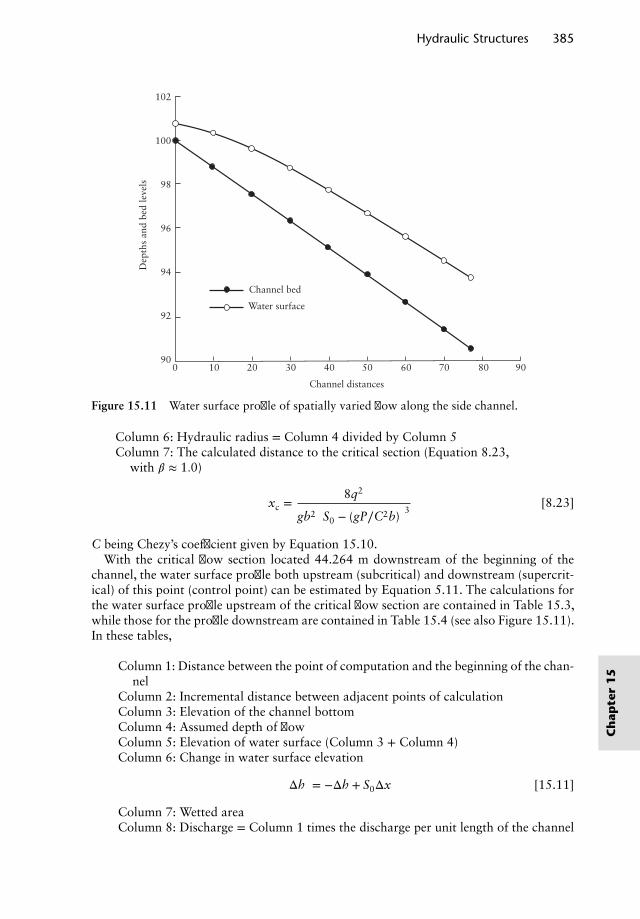
Hydraulic Structures 385
0 10 20 30 40 50 60 70 80 90
Channel distances
Channel bed
Water surface
Dep
ths
and
bed
leve
ls
102
100
98
96
94
92
90
Figure 15.11 Water surface profile of spatially varied flow along the side channel.
Column 6: Hydraulic radius = Column 4 divided by Column 5Column 7: The calculated distance to the critical section (Equation 8.23,
with 𝛽 ≈ 1.0)
xc =8q2
gb2[S0 − (gP∕C2b)
]3[8.23]
C being Chezy’s coefficient given by Equation 15.10.With the critical flow section located 44.264 m downstream of the beginning of the
channel, the water surface profile both upstream (subcritical) and downstream (supercrit-ical) of this point (control point) can be estimated by Equation 5.11. The calculations forthe water surface profile upstream of the critical flow section are contained in Table 15.3,while those for the profile downstream are contained in Table 15.4 (see also Figure 15.11).In these tables,
Column 1: Distance between the point of computation and the beginning of the chan-nel
Column 2: Incremental distance between adjacent points of calculationColumn 3: Elevation of the channel bottomColumn 4: Assumed depth of flowColumn 5: Elevation of water surface (Column 3 + Column 4)Column 6: Change in water surface elevation
Δh′ = −Δh + S0Δx [15.11]
Column 7: Wetted areaColumn 8: Discharge = Column 1 times the discharge per unit length of the channel
Ch
apte
r1
5
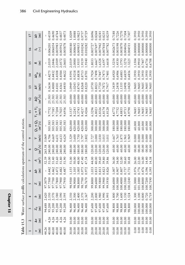
386 Civil Engineering Hydraulics
Tab
le15
.3W
ater
surf
ace
profi
leca
lcul
atio
nsup
stre
amof
the
cont
rols
ecti
on.
12
34
56
78
910
1112
1314
1516
17
x𝚫x
Z0
hZ
𝚫h′
AQ
VQ
1+
Q2
V1+
V2
𝚫Q𝚫V
𝚫h′ m
RS f
𝚫h′
(m)
(m)
(m)
(m)
(m)
(m)
(m2)
(m3∕s
)(m
/s)
(m3∕s
)(m
/s)
(m3∕s
)(m
/s)
(m)
(m)
(−)
(m)
44.2
6–
94.6
882.
620
97.3
079
–52
.39
265.
585.
069
––
––
––
––
40.0
04.
2695
.200
2.55
097
.750
00.
442
51.0
024
0.00
4.70
650
5.58
39.
7752
25.5
830.
3634
0.42
752.
0319
0.00
6201
0.45
3940
.00
4.26
95.2
002.
570
97.7
700
0.46
251
.40
240.
004.
669
505.
583
9.73
8525
.583
0.40
000.
4432
2.04
460.
0060
540.
4690
40.0
04.
2695
.200
2.58
097
.780
00.
472
51.6
024
0.00
4.65
150
5.58
39.
7204
25.5
830.
4181
0.45
082.
0509
0.00
5983
0.47
6440
.00
4.26
95.2
002.
590
97.7
900
0.48
251
.80
240.
004.
633
505.
583
9.70
2525
.583
0.43
610.
4584
2.05
720.
0059
120.
4837
40.0
04.
2695
.200
2.59
597
.795
00.
487
51.9
024
0.00
4.62
450
5.58
39.
6936
25.5
830.
4450
0.46
222.
0603
0.00
5878
0.48
73
30.0
010
.00
96.4
002.
550
98.9
500
1.15
551
.00
180.
003.
529
420.
000
8.15
3760
.000
1.09
490.
9391
2.03
190.
0081
801.
0209
30.0
010
.00
96.4
002.
500
98.9
000
1.10
550
.00
180.
003.
600
420.
000
8.22
4360
.000
1.02
430.
9218
2.00
000.
0086
921.
0088
30.0
010
.00
96.4
002.
400
98.8
000
1.00
548
.00
180.
003.
750
420.
000
8.37
4360
.000
0.87
430.
8838
1.93
550.
0098
530.
9823
30.0
010
.00
96.4
002.
370
98.7
700
0.97
547
.40
180.
003.
797
420.
000
8.42
1760
.000
0.82
680.
8713
1.91
590.
0102
420.
9737
30.0
010
.00
96.4
002.
367
98.7
670
0.97
247
.34
180.
003.
802
420.
000
8.42
6660
.000
0.82
200.
8701
1.91
400.
0102
820.
9729
20.0
010
.00
97.6
002.
200
99.8
000
1.03
344
.00
120.
002.
727
300.
000
6.52
9660
.000
1.07
500.
7924
1.80
330.
0057
270.
8496
20.0
010
.00
97.6
002.
000
99.6
000
0.83
340
.00
120.
003.
000
300.
000
6.80
2360
.000
0.80
230.
7498
1.66
670.
0076
970.
8268
20.0
010
.00
97.6
001.
980
99.5
800
0.81
339
.60
120.
003.
030
300.
000
6.83
2660
.000
0.77
200.
7447
1.65
280.
0079
420.
8241
20.0
010
.00
97.6
001.
990
99.5
900
0.82
339
.80
120.
003.
015
300.
000
6.81
7460
.000
0.78
720.
7473
1.65
970.
0078
180.
8255
20.0
010
.00
97.6
001.
993
99.5
930
0.82
639
.86
120.
003.
011
300.
000
6.81
2860
.000
0.79
170.
7481
1.66
180.
0077
820.
8259
10.0
010
.00
98.8
001.
800
100.
6000
1.00
736
.00
60.0
01.
667
180.
000
4.67
7260
.000
1.34
390.
6920
1.52
540.
0026
730.
7188
10.0
010
.00
98.8
001.
700
100.
5000
0.90
734
.00
60.0
01.
765
180.
000
4.77
5260
.000
1.24
580.
6906
1.45
300.
0031
980.
7226
10.0
010
.00
98.8
001.
600
100.
4000
0.80
732
.00
60.0
01.
875
180.
000
4.88
5560
.000
1.13
550.
6883
1.37
930.
0038
700.
7270
10.0
010
.00
98.8
001.
530
100.
3300
0.73
730
.60
60.0
01.
961
180.
000
4.97
1360
.000
1.04
980.
6859
1.32
700.
0044
560.
7304
10.0
010
.00
98.8
001.
524
100.
3240
0.73
130
.48
60.0
01.
969
180.
000
4.97
9060
.000
1.04
200.
6856
1.32
250.
0045
110.
7307
0.00
10.0
010
0.00
01.
300
101.
3000
0.97
626
.00
00.0
00.
000
60.0
001.
9685
60.0
001.
9685
0.39
501.
1504
0.00
0000
0.39
500.
0010
.00
100.
000
1.10
010
1.10
000.
776
22.0
000
.00
0.00
060
.000
1.96
8560
.000
1.96
850.
3950
0.99
100.
0000
000.
3950
0.00
10.0
010
0.00
00.
800
100.
8000
0.47
616
.00
00.0
00.
000
60.0
001.
9685
60.0
001.
9685
0.39
500.
7407
0.00
0000
0.39
500.
0010
.00
100.
000
0.72
010
0.72
000.
396
14.4
000
.00
0.00
060
.000
1.96
8560
.000
1.96
850.
3950
0.67
160.
0000
000.
3950
0.00
10.0
010
0.00
00.
719
100.
7190
0.39
514
.38
00.0
00.
000
60.0
001.
9685
60.0
001.
9685
0.39
500.
6708
0.00
0000
0.39
50
Ch
apter
15
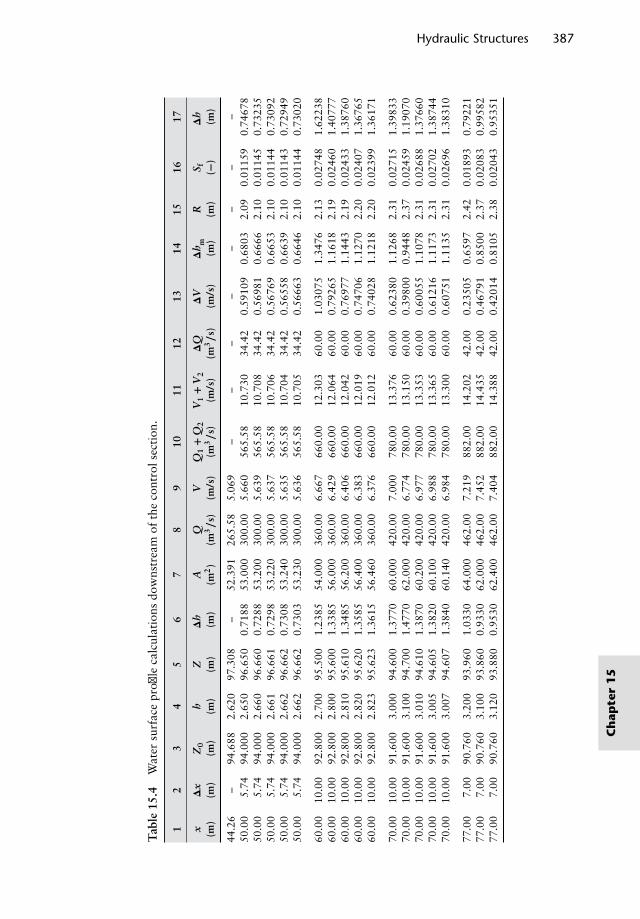
Hydraulic Structures 387
Tab
le15
.4W
ater
surf
ace
profi
leca
lcul
atio
nsdo
wns
trea
mof
the
cont
rols
ecti
on.
12
34
56
78
910
1112
1314
1516
17
x𝚫x
Z0
hZ
𝚫h′
AQ
VQ
1+
Q2
V1+
V2
𝚫Q𝚫V
𝚫h′ m
RS f
𝚫h′
(m)
(m)
(m)
(m)
(m)
(m)
(m2)
(m3∕s
)(m
/s)
(m3∕s
)(m
/s)
(m3∕s
)(m
/s)
(m)
(m)
(−)
(m)
44.2
6–
94.6
882.
620
97.3
08–
52.3
9126
5.58
5.06
9–
––
––
––
–50
.00
5.74
94.0
002.
650
96.6
500.
7188
53.0
0030
0.00
5.66
056
5.58
10.7
3034
.42
0.59
109
0.68
032.
090.
0115
90.
7467
850
.00
5.74
94.0
002.
660
96.6
600.
7288
53.2
0030
0.00
5.63
956
5.58
10.7
0834
.42
0.56
981
0.66
662.
100.
0114
50.
7323
550
.00
5.74
94.0
002.
661
96.6
610.
7298
53.2
2030
0.00
5.63
756
5.58
10.7
0634
.42
0.56
769
0.66
532.
100.
0114
40.
7309
250
.00
5.74
94.0
002.
662
96.6
620.
7308
53.2
4030
0.00
5.63
556
5.58
10.7
0434
.42
0.56
558
0.66
392.
100.
0114
30.
7294
950
.00
5.74
94.0
002.
662
96.6
620.
7303
53.2
3030
0.00
5.63
656
5.58
10.7
0534
.42
0.56
663
0.66
462.
100.
0114
40.
7302
0
60.0
010
.00
92.8
002.
700
95.5
001.
2385
54.0
0036
0.00
6.66
766
0.00
12.3
0360
.00
1.03
075
1.34
762.
130.
0274
81.
6223
860
.00
10.0
092
.800
2.80
095
.600
1.33
8556
.000
360.
006.
429
660.
0012
.064
60.0
00.
7926
51.
1618
2.19
0.02
460
1.40
777
60.0
010
.00
92.8
002.
810
95.6
101.
3485
56.2
0036
0.00
6.40
666
0.00
12.0
4260
.00
0.76
977
1.14
432.
190.
0243
31.
3876
060
.00
10.0
092
.800
2.82
095
.620
1.35
8556
.400
360.
006.
383
660.
0012
.019
60.0
00.
7470
61.
1270
2.20
0.02
407
1.36
765
60.0
010
.00
92.8
002.
823
95.6
231.
3615
56.4
6036
0.00
6.37
666
0.00
12.0
1260
.00
0.74
028
1.12
182.
200.
0239
91.
3617
1
70.0
010
.00
91.6
003.
000
94.6
001.
3770
60.0
0042
0.00
7.00
078
0.00
13.3
7660
.00
0.62
380
1.12
682.
310.
0271
51.
3983
370
.00
10.0
091
.600
3.10
094
.700
1.47
7062
.000
420.
006.
774
780.
0013
.150
60.0
00.
3980
00.
9448
2.37
0.02
459
1.19
070
70.0
010
.00
91.6
003.
010
94.6
101.
3870
60.2
0042
0.00
6.97
778
0.00
13.3
5360
.00
0.60
055
1.10
782.
310.
0268
81.
3766
070
.00
10.0
091
.600
3.00
594
.605
1.38
2060
.100
420.
006.
988
780.
0013
.365
60.0
00.
6121
61.
1173
2.31
0.02
702
1.38
744
70.0
010
.00
91.6
003.
007
94.6
071.
3840
60.1
4042
0.00
6.98
478
0.00
13.3
0060
.00
0.60
751
1.11
352.
310.
0269
61.
3831
0
77.0
07.
0090
.760
3.20
093
.960
1.03
3064
.000
462.
007.
219
882.
0014
.202
42.0
00.
2350
50.
6597
2.42
0.01
893
0.79
221
77.0
07.
0090
.760
3.10
093
.860
0.93
3062
.000
462.
007.
452
882.
0014
.435
42.0
00.
4679
10.
8500
2.37
0.02
083
0.99
582
77.0
07.
0090
.760
3.12
093
.880
0.95
3062
.400
462.
007.
404
882.
0014
.388
42.0
00.
4201
40.
8105
2.38
0.02
043
0.95
351
Ch
apte
r1
5
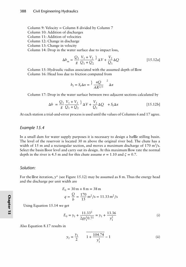
388 Civil Engineering Hydraulics
Column 9: Velocity = Column 8 divided by Column 7Column 10: Addition of dischargesColumn 11: Addition of velocitiesColumn 12: Change in dischargeColumn 13: Change in velocityColumn 14: Drop in the water surface due to impact loss,
Δh′m =
Q1
gV1 + V2
Q1 + Q2
(ΔV +
V2
Q1ΔQ
)[15.12a]
Column 15: Hydraulic radius associated with the assumed depth of flowColumn 16: Head loss due to friction computed from
hf = SfΔx =(
nQ
AR2∕3
)2
Δx
Column 17: Drop in the water surface between two adjacent sections calculated by
Δh′ =Q1
gV1 + V2
Q1 + Q2
(ΔV +
V2
Q1ΔQ
)+ SfΔx [15.12b]
At each station a trial-and-error process is used until the values of Columns 6 and 17 agree.
Example 15.4
In a small dam for water supply purposes it is necessary to design a baffle stilling basin.The level of the reservoir is located 30 m above the original river bed. The chute has awidth of 15 m and a rectangular section, and moves a maximum discharge of 170 m3∕s.Select the basin floor level and carry out its design. At this maximum flow rate the normaldepth in the river is 4.5 m and for this chute assume 𝜎 = 1.10 and 𝜁 = 0.7.
Solution:
For the first iteration, y+ (see Figure 15.12) may be assumed as 8 m. Thus the energy headand the discharge per unit width are
E0 = 30 m + 8 m = 38 m
q =Q
b= 170
15m2∕s = 11.33 m2∕s
Using Equation 15.14 we get
E0 = y1 +11.332
2gy210.72
= y1 +13.36
y21
(i)
Also Equation 8.17 results in
y2 =y1
2
(√1 + 104.74
y31
− 1
)(ii)
Ch
apter
15
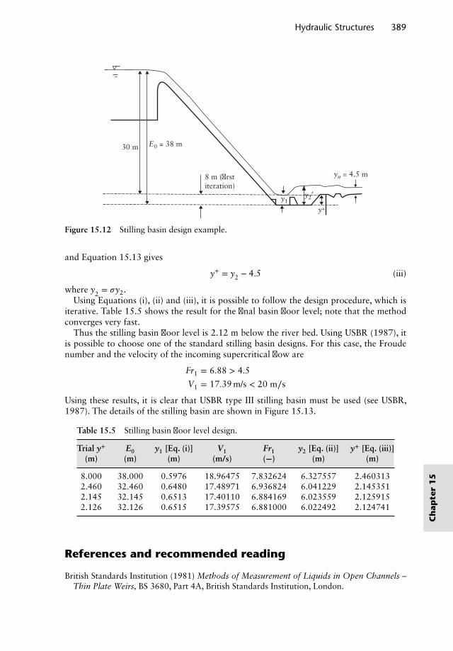
Hydraulic Structures 389
30 m
8 m (firstiteration)
E0 = 38 m
yn = 4.5 m
y2′ y1
y+
Figure 15.12 Stilling basin design example.
and Equation 15.13 gives
y+ = y′2 − 4.5 (iii)
where y′2 = 𝜎y2.Using Equations (i), (ii) and (iii), it is possible to follow the design procedure, which is
iterative. Table 15.5 shows the result for the final basin floor level; note that the methodconverges very fast.
Thus the stilling basin floor level is 2.12 m below the river bed. Using USBR (1987), itis possible to choose one of the standard stilling basin designs. For this case, the Froudenumber and the velocity of the incoming supercritical flow are
Fr1 = 6.88 > 4.5
V1 = 17.39 m/s < 20 m∕s
Using these results, it is clear that USBR type III stilling basin must be used (see USBR,1987). The details of the stilling basin are shown in Figure 15.13.
Table 15.5 Stilling basin floor level design.
Trial y+ E0 y1 [Eq. (i)] V1 Fr1 y2 [Eq. (ii)] y+ [Eq. (iii)](m) (m) (m) (m/s) (−) (m) (m)
8.000 38.000 0.5976 18.96475 7.832624 6.327557 2.4603132.460 32.460 0.6480 17.48971 6.936824 6.041229 2.1453512.145 32.145 0.6513 17.40110 6.884169 6.023559 2.1259152.126 32.126 0.6515 17.39575 6.881000 6.022492 2.124741
References and recommended reading
British Standards Institution (1981) Methods of Measurement of Liquids in Open Channels –Thin Plate Weirs, BS 3680, Part 4A, British Standards Institution, London.
Ch
apte
r1
5
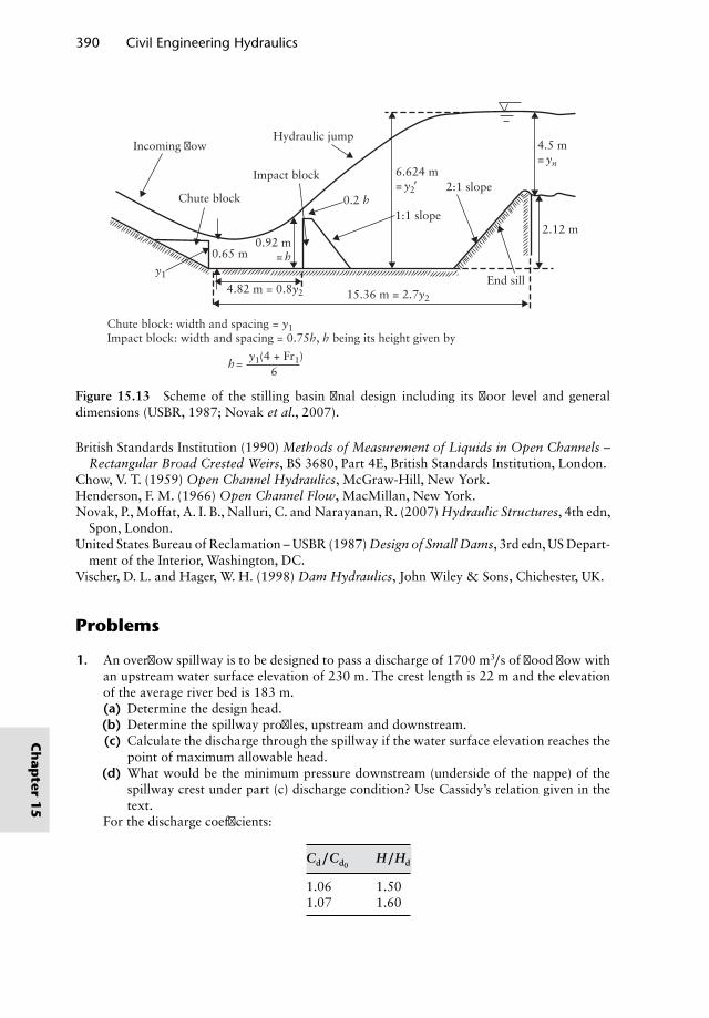
390 Civil Engineering Hydraulics
Incoming flowHydraulic jump
Impact block
1:1 slope
2:1 slope
End sill
2.12 m
Chute block
6
Chute block: width and spacing = y1Impact block: width and spacing = 0.75h, h being its height given by
h=
0.92 m= h
6.624 m= y2′
4.5 m= yn
15.36 m = 2.7y2
y1
y1(4 + Fr1)
4.82 m = 0.8y2
0.65 m
0.2 h
Figure 15.13 Scheme of the stilling basin final design including its floor level and generaldimensions (USBR, 1987; Novak et al., 2007).
British Standards Institution (1990) Methods of Measurement of Liquids in Open Channels –Rectangular Broad Crested Weirs, BS 3680, Part 4E, British Standards Institution, London.
Chow, V. T. (1959) Open Channel Hydraulics, McGraw-Hill, New York.Henderson, F. M. (1966) Open Channel Flow, MacMillan, New York.Novak, P., Moffat, A. I. B., Nalluri, C. and Narayanan, R. (2007) Hydraulic Structures, 4th edn,
Spon, London.United States Bureau of Reclamation – USBR (1987) Design of Small Dams, 3rd edn, US Depart-
ment of the Interior, Washington, DC.Vischer, D. L. and Hager, W. H. (1998) Dam Hydraulics, John Wiley & Sons, Chichester, UK.
Problems
1. An overflow spillway is to be designed to pass a discharge of 1700 m3∕s of flood flow withan upstream water surface elevation of 230 m. The crest length is 22 m and the elevationof the average river bed is 183 m.(a) Determine the design head.(b) Determine the spillway profiles, upstream and downstream.(c) Calculate the discharge through the spillway if the water surface elevation reaches the
point of maximum allowable head.(d) What would be the minimum pressure downstream (underside of the nappe) of the
spillway crest under part (c) discharge condition? Use Cassidy’s relation given in thetext.
For the discharge coefficients:
Cd∕Cd0H∕Hd
1.06 1.501.07 1.60
Ch
apter
15
Hydraulic Structures 391
2. If the spillway of Problem 1 is required to have piers to support a bridge deck over it and ifthe maximum free span between them is 6.3 m, what would be the discharge correspondingto the design head? What is the new allowable maximum discharge? The pier coefficientis 0.011, and the abutment contraction coefficient is 0.12.
3. A trapezoidal lateral spillway channel 127 m long is designed to carry a discharge whichincreases at a rate of 11 m3∕(s m). The cross section has a bottom width of 18 m andlateral slopes of 2 (vertical) : 1 (horizontal). The longitudinal slope of the channel is 0.08and starts at an upstream elevation of 520 m. If Manning’s n is equal to 0.014 (concrete),determine if there is a critical section and the corresponding water surface profile.
4. A hydraulic jump stilling basin is to be designed to dissipate the energy of a maximumdischarge of 750 m3∕s. The water surface in the upstream reservoir is located at a level of350 m. The chute channel has a slope of 45◦, rectangular in cross section with a width of22.5 m. At this discharge the river downstream of the basin has a normal depth of 4.4 m,and the bed is located at an elevation of 307 m. For this chute 𝜎 = 1.05 and 𝜁 = 0.75.(a) Determine the sequent depth of the hydraulic jump and the bed level of the stilling
basin.(b) Choose the stilling basin design according to the USBR (1987) standards. Make a
sketch of the basin.(c) Determine the percentage of energy dissipation in the basin.
Ch
apte
r1
5

Chapter 16Environmental Hydraulicsand Engineering Hydrology
16.1 Introduction
This chapter extends the discussion from previous chapters to cover wider issues con-cerning water in the environment and presents some further worked examples relevant toenvironmental engineering topics, with a particular theme of flood alleviation.
The well-known natural hydrological cycle traces the path of rainfall as it results ininfiltration to the ground, surface runoff, evaporation and transpiration from trees andplants, returning to clouds and resulting in further rainfall. Alongside this, there is also acycle of human use of water. Water in the environment is impounded by dams or pumpedfrom the ground, treated for human consumption, distributed through pipes and channelsfor drinking and irrigation purposes, collected after use by sewerage systems and returnedto the environment usually after suitable treatment. Many of the theories and calculationtechniques from previous chapters find useful applications at different points in these cyclesand enable engineers to analyse and design works to manage water in the environment.
Management of water has increasingly been recognised as involving environmentaland sustainability issues, with particular concerns arising from urbanisation and climatechange which have a bearing on flood risk management. Recommended reading includesmore extended treatment of such topics, whilst the following sections serve to introducethe worked examples.
16.2 Analysis of gauged river flow data
Much of hydrology is concerned with analysis of data. Where river discharges are required,it is considered preferable where possible to work with actual discharge data, rather thanto deduce results from rainfall and catchment characteristics. The latter approach may beneeded where reliable discharge data are not available, and reference for this can be madeto more specialised texts in the recommended reading. The analysis that follows illustratesthe former approach where gauged records of discharge values are available.
Nalluri & Featherstone’s Civil Engineering Hydraulics: Essential Theory with Worked Examples,Sixth Edition. Martin Marriott.© 2016 John Wiley & Sons, Ltd. Published 2016 by John Wiley & Sons, Ltd.Companion Website: www.wiley.com/go/Marriott
394 Civil Engineering Hydraulics
For gauged catchments, a time series of measured annual maximum discharge valuesmay be analysed to provide values with particular probabilities for design purposes. Themeasured data may come from a weir or flume, as described in Chapter 8, or from anultrasonic gauging station or other velocity–area method. The annual exceedance proba-bility P is related to the annual probability of non-exceedance F and to the return periodT years by the following expression:
P = 1 − F = 1T
[16.1]
Return period T has been widely used to express the average time interval betweenevents greater than or equal to the value specified. However, this term has been criticisedfor implying a periodic regularity, which is not the case in reality (see Fleming, 2002).
Having ranked the annual maximum data for N years, in descending order from greatesti = 1 to least i = N, each point may be assigned a value of P from a formula of the form
P = i − aN + b
[16.2]
where a and b are constants depending on the probability distribution of the data. Alter-natively, if ranked ascending from least with j = 1 to greatest with j = N, such a formulaproduces the annual probability of non-exceedance:
F =j − a
N + b[16.3]
From the two approaches to ranking, either in descending order i or in ascending orderj, it is noted that
i + j = N + 1 [16.4]
A combination of Equations 16.1–16.4 then yields the result
b = 1 − 2a [16.5]
Widely used values include a = 0 (Weibull) and a = 0.44 (Gringorten), with the lattergenerally preferred for extreme value distributions. The Gringorten plotting position for-mula for exceedance probability P is thus
P = i − 0.44N + 0.12
[16.6]
and the non-exceedance probability F may be calculated either from Equation 16.1 orfrom ranked data:
F =j − 0.44
N + 0.12[16.7]
For a two-parameter analysis, a straight line may be fitted to the points plotted againstan appropriate reduced variate. One such is the Gumbel reduced variate:
yG = − ln(− ln(F)) [16.8]
This relates to the extreme value type 1 (EV1) distribution, for which the cumulativedistribution function F(x) is
F(x) = e−e−[(x−u)∕𝛼][16.9]
Ch
apter
16
Environmental Hydraulics and Engineering Hydrology 395
Hence, when values of flow rate Q are plotted as the variable x against the Gumbelreduced variate yG, we have the straight-line relationship
Q = u + 𝛼yG [16.10]
The parameters u and 𝛼 may be found approximately by a best-fit line through thedisplayed data or estimated by a method of moments drawing on the properties of the EV1distribution, using the mean (𝜇) and sample standard deviation (s) of the data as follows:
u = 𝜇 − 0.45s [16.11]
and
𝛼 = 0.78s [16.12]
This is shown in Example 16.1 using the River Thames data.An alternative approach recommended in the Flood Estimation Handbook (Institute of
Hydrology, 1999) advocates the use of the generalised logistic distribution, and data aredisplayed using the logistic reduced variate
yL = −ln(
1 − FF
)[16.13]
In this approach, the flow rates Q are non-dimensionalised using the median annualmaximum flood QMED, and related to the following growth curve:
QQMED
= 1 + 𝛽
k
[1 −
(1 − F
F
)k]
[16.14]
Values of k and 𝛽 are estimated by a method using L moments, illustrated in Example16.2 using the River Thames data, and this method is considered more appropriate forskewed data. In the special case of k = 0, the two-parameter logistic distribution is usedwith
QQMED
= 1 + 𝛽yL [16.15]
Space does not permit a fuller discussion here of the details of this method, or other rec-ommended procedures such as the pooling of data from hydrologically similar catchmentsto extend the amount of data (see Institute of Hydrology, 1999, volume 3). The compari-son of Examples 16.1 and 16.2 usefully illustrates how the results depend on the methodof analysis, as well as demonstrates the methods involved.
16.3 River Thames discharge data
For the worked examples that follow, 120 years of published Thames discharge data areused for illustration, and some comments follow on the data which serve to indicate someof the issues associated with such data series. These data for the water years 1884–2003are presented by Herschy (2003, 2004), with the Thames data updated and corrected in thelater supplement dated 2004. These data are the highest daily mean flows (for the hydro-logical day 0900–0900 hours) for each water year (October to September) and have beennaturalised (adjusted to account for major upstream abstractions). For large river basinsworldwide, the mean daily value is usually not significantly different from the instanta-neous maximum value, and peak flows quoted are often daily mean flows. However in the
Ch
apte
r1
6
396 Civil Engineering Hydraulics
UK, catchment response times are usually such that instantaneous or 15 minute peak flowdata are generally used (Institute of Hydrology, 1999), hence the reason for noting thispoint. Herschy (2003) advises that for these Thames data, instantaneous peak flows canby estimated by increasing the quoted daily mean values by 2–5%. One further commenton the data used is that the earlier records are from Teddington Weir, whereas since 1977,data have been recorded at an ultrasonic gauging station at Kingston; as noted in Marshet al. (2005), this is still considered as one continuous series, due to the negligible differencein catchment areas. The inherent assumption of hydrological stationarity remains that thedata do not contain a significant trend over time from a cause such as climate change.The examples that follow are analysed on that basis, and the present pragmatic advice inthis context concerning effects of climate change is to investigate the sensitivity of futuredesigns to the addition of a percentage to predicted peak river flows to allow for suchfuture changes.
16.4 Flood alleviation, sustainability andenvironmental channels
The main components of constructed works to alleviate the effects of flooding are the pro-vision of storage, the increase in channel conveyance capacity and the provision of protec-tion by means of banks or walls. Other measures include better warning and emergencyplanning.
One of the main components of sustainable urban drainage systems is to provide stor-age near to the source, by use of swales, permeable pavements and tank sewers. Advicefor developers on such issues is now included in such publications as Water UK (2012).Storage can also be beneficial and cost-effective on larger rural catchments, as provided,for example, by the use of check dams on tributaries. The flood routing in Example 11.8has demonstrated the beneficial effect of storage on reducing the magnitude of the peakof a flood hydrograph, as illustrated in Figure 11.6.
Sustainability in a broad sense involves balancing the effects of economic, social andenvironmental constraints, and places the traditional engineering concerns of quality, costand time within a complex framework of other issues (see Fenner et al., 2006). The trendin river engineering works has been to maintain to a greater extent the natural featuresof channels, with sediment transport issues as discussed in Chapter 14 being of particularsignificance.
Section 8.4 and Example 8.6 demonstrated the properties of a two-stage channel, andthis combination of river and flood plain provides the combined conveyance for a valley.Often the main channel meanders within the flood plain, and there has been a growingconcern to maintain such features. The degree of meandering is measured by the sinuositys, which is defined in relation to the length L or slope S of the flood plain (subscript ‘F’)and the main channel (subscript ‘C’) as follows:
s =LC
LF=
SF
SC[16.16]
In a simple one-dimensional approach, the discharge equation may be adjusted for ameandering channel to allow for the different hydraulic gradients on the channel andflood plain components of the flow, for example using the Manning formula,
Q =AF
nFR2∕3
F S1∕2F +
AC
nCR2∕3
C S1∕2C [16.17]
Ch
apter
16
Environmental Hydraulics and Engineering Hydrology 397
but the previous vertical division between flood plain and main channel shown inFigure 8.3 becomes less appropriate as the degree of meandering increases.
The complex nature of interaction between the components is the subject of ongoingresearch beyond the scope of this text, concerning not only the conveyance but also thesediment transport (see e.g. Loveless et al., 2000).
16.5 Project appraisal
A final section is included on the appraisal of schemes such as those for flood allevia-tion, using cost–benefit analysis. The discounted cash flow approach is used to express thepresent values of costs and benefits that arise at different points in time. Benefits need tobe expressed in cost terms, and represent desirable consequences of the project, and tech-niques exist to help to quantify and include non-tangible and environmental benefits, aswell as those that simply relate to the prevention of damage in monetary terms. All costs areexpressed at present price levels, and a discount rate r is selected, which reflects the extentto which positive benefits are preferred sooner rather than later, and adverse or undesirablecosts later rather than sooner. For a single sum arising at the end of year n in the future,the appropriate factor is the inverse of the well-known formula for compound interest.
Single sum factor = (1 + r)−n [16.18]
Hence the present value of sum X arising at the end of the year n
= X(1 + r)−n [16.19]
For a regular stream of annual sums at the end of each year, the cumulative present valuefactor is given by
Cumulative factor =n∑
i=1
(1 + r)−i = 1 − (1 + r)−n
r[16.20]
Hence the present value of annual sums Y for n years = Y(
1 − (1 + r)−n
r
)[16.21]
The formula for the cumulative present value factor is derived using the mathematicaltechnique for summing a geometric progression, and may be seen to tend to the limit of 1/ras n tends to infinity. Sometimes that simplification is taken, but more usually a value of n isset for the design life of the scheme, which it should be noted may well differ from the levelof protection provided and from the asset lives of the various components of the scheme.
Costs are often a mix of capital and annual running or maintenance costs, to whichEquations 16.19 and 16.21 would apply, respectively. Benefits arising from the damageprevented are assessed over the design life of the scheme as the stream of annual expectedbenefits, using the cumulative present value factor approach as in Equation 16.21. Theannual expected benefit is calculated from combining the damage and probability data, asillustrated in Example 16.3. It should be noted that as well as the damage that has beenprevented, there may also be other benefits, such as the opening up of areas for recreationsuch as riverside footpaths, which could be valued using willingness to pay or contingentvaluation methods (see e.g. Penning-Rowsell and Green, 2000, for a discussion of theseand other issues, such as above-design-standard benefits).
Having established the present value of benefits B and the present value of costs C,these may be compared as the benefit-to-cost ratio B/C, and values exceeding 1 show thatthe scheme may be justified in this way. The calculation approach above is illustrated inExample 16.3.
Ch
apte
r1
6
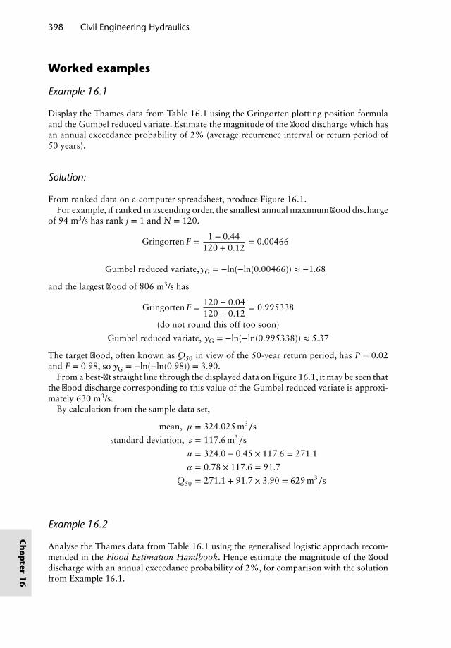
398 Civil Engineering Hydraulics
Worked examples
Example 16.1
Display the Thames data from Table 16.1 using the Gringorten plotting position formulaand the Gumbel reduced variate. Estimate the magnitude of the flood discharge which hasan annual exceedance probability of 2% (average recurrence interval or return period of50 years).
Solution:
From ranked data on a computer spreadsheet, produce Figure 16.1.For example, if ranked in ascending order, the smallest annual maximum flood discharge
of 94 m3/s has rank j = 1 and N = 120.
Gringorten F = 1 − 0.44120 + 0.12
= 0.00466
Gumbel reduced variate,yG = −ln(−ln(0.00466)) ≈ −1.68
and the largest flood of 806 m3/s has
Gringorten F = 120 − 0.04120 + 0.12
= 0.995338
(do not round this off too soon)
Gumbel reduced variate, yG = −ln(−ln(0.995338)) ≈ 5.37
The target flood, often known as Q50 in view of the 50-year return period, has P = 0.02and F = 0.98, so yG = −ln(−ln(0.98)) = 3.90.
From a best-fit straight line through the displayed data on Figure 16.1, it may be seen thatthe flood discharge corresponding to this value of the Gumbel reduced variate is approxi-mately 630 m3/s.
By calculation from the sample data set,
mean, 𝜇 = 324.025 m3∕s
standard deviation, s = 117.6 m3∕s
u = 324.0 − 0.45 × 117.6 = 271.1
𝛼 = 0.78 × 117.6 = 91.7
Q50 = 271.1 + 91.7 × 3.90 = 629 m3∕s
Example 16.2
Analyse the Thames data from Table 16.1 using the generalised logistic approach recom-mended in the Flood Estimation Handbook. Hence estimate the magnitude of the flooddischarge with an annual exceedance probability of 2%, for comparison with the solutionfrom Example 16.1.
Ch
apter
16
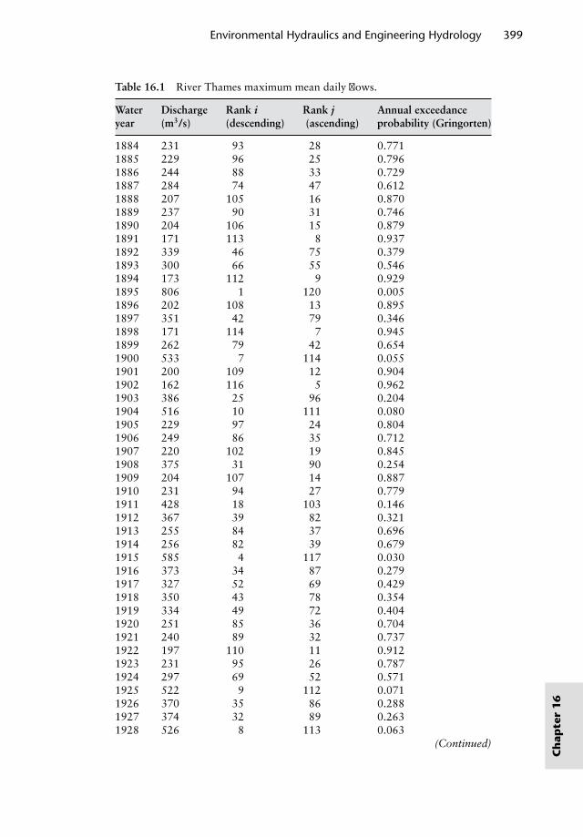
Environmental Hydraulics and Engineering Hydrology 399
Table 16.1 River Thames maximum mean daily flows.
Water Discharge Rank i Rank j Annual exceedanceyear (m3/s) (descending) (ascending) probability (Gringorten)
1884 231 93 28 0.7711885 229 96 25 0.7961886 244 88 33 0.7291887 284 74 47 0.6121888 207 105 16 0.8701889 237 90 31 0.7461890 204 106 15 0.8791891 171 113 8 0.9371892 339 46 75 0.3791893 300 66 55 0.5461894 173 112 9 0.9291895 806 1 120 0.0051896 202 108 13 0.8951897 351 42 79 0.3461898 171 114 7 0.9451899 262 79 42 0.6541900 533 7 114 0.0551901 200 109 12 0.9041902 162 116 5 0.9621903 386 25 96 0.2041904 516 10 111 0.0801905 229 97 24 0.8041906 249 86 35 0.7121907 220 102 19 0.8451908 375 31 90 0.2541909 204 107 14 0.8871910 231 94 27 0.7791911 428 18 103 0.1461912 367 39 82 0.3211913 255 84 37 0.6961914 256 82 39 0.6791915 585 4 117 0.0301916 373 34 87 0.2791917 327 52 69 0.4291918 350 43 78 0.3541919 334 49 72 0.4041920 251 85 36 0.7041921 240 89 32 0.7371922 197 110 11 0.9121923 231 95 26 0.7871924 297 69 52 0.5711925 522 9 112 0.0711926 370 35 86 0.2881927 374 32 89 0.2631928 526 8 113 0.063
(Continued)
Ch
apte
r1
6
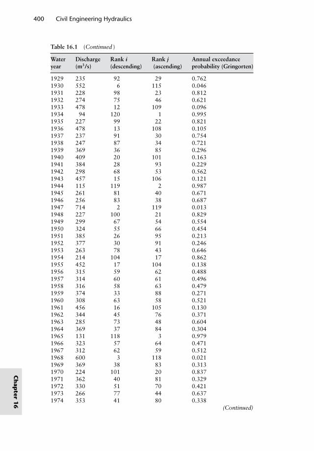
400 Civil Engineering Hydraulics
Table 16.1 (Continued )
Water Discharge Rank i Rank j Annual exceedanceyear (m3/s) (descending) (ascending) probability (Gringorten)
1929 235 92 29 0.7621930 552 6 115 0.0461931 228 98 23 0.8121932 274 75 46 0.6211933 478 12 109 0.0961934 94 120 1 0.9951935 227 99 22 0.8211936 478 13 108 0.1051937 237 91 30 0.7541938 247 87 34 0.7211939 369 36 85 0.2961940 409 20 101 0.1631941 384 28 93 0.2291942 298 68 53 0.5621943 457 15 106 0.1211944 115 119 2 0.9871945 261 81 40 0.6711946 256 83 38 0.6871947 714 2 119 0.0131948 227 100 21 0.8291949 299 67 54 0.5541950 324 55 66 0.4541951 385 26 95 0.2131952 377 30 91 0.2461953 263 78 43 0.6461954 214 104 17 0.8621955 452 17 104 0.1381956 315 59 62 0.4881957 314 60 61 0.4961958 316 58 63 0.4791959 374 33 88 0.2711960 308 63 58 0.5211961 456 16 105 0.1301962 344 45 76 0.3711963 285 73 48 0.6041964 369 37 84 0.3041965 131 118 3 0.9791966 323 57 64 0.4711967 312 62 59 0.5121968 600 3 118 0.0211969 369 38 83 0.3131970 224 101 20 0.8371971 362 40 81 0.3291972 330 51 70 0.4211973 266 77 44 0.6371974 353 41 80 0.338
(Continued)
Ch
apter
16
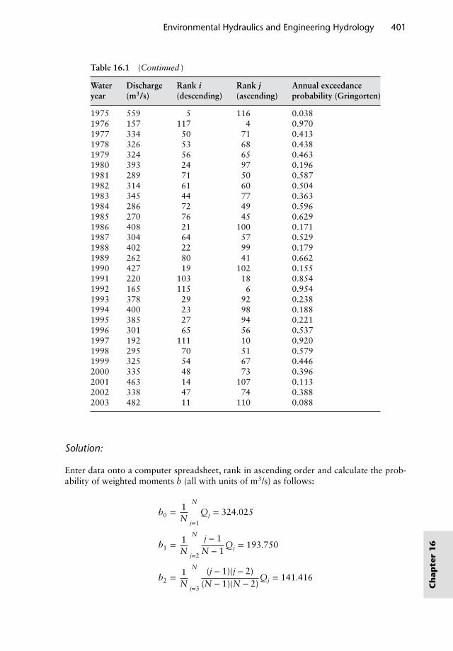
Environmental Hydraulics and Engineering Hydrology 401
Table 16.1 (Continued )
Water Discharge Rank i Rank j Annual exceedanceyear (m3/s) (descending) (ascending) probability (Gringorten)
1975 559 5 116 0.0381976 157 117 4 0.9701977 334 50 71 0.4131978 326 53 68 0.4381979 324 56 65 0.4631980 393 24 97 0.1961981 289 71 50 0.5871982 314 61 60 0.5041983 345 44 77 0.3631984 286 72 49 0.5961985 270 76 45 0.6291986 408 21 100 0.1711987 304 64 57 0.5291988 402 22 99 0.1791989 262 80 41 0.6621990 427 19 102 0.1551991 220 103 18 0.8541992 165 115 6 0.9541993 378 29 92 0.2381994 400 23 98 0.1881995 385 27 94 0.2211996 301 65 56 0.5371997 192 111 10 0.9201998 295 70 51 0.5791999 325 54 67 0.4462000 335 48 73 0.3962001 463 14 107 0.1132002 338 47 74 0.3882003 482 11 110 0.088
Solution:
Enter data onto a computer spreadsheet, rank in ascending order and calculate the prob-ability of weighted moments b (all with units of m3/s) as follows:
b0 = 1N
N∑j=1
Qj = 324.025
b1 = 1N
N∑j=2
j − 1N − 1
Qj = 193.750
b2 = 1N
N∑j=3
(j − 1)(j − 2)(N − 1)(N − 2)
Qj = 141.416
Ch
apte
r1
6
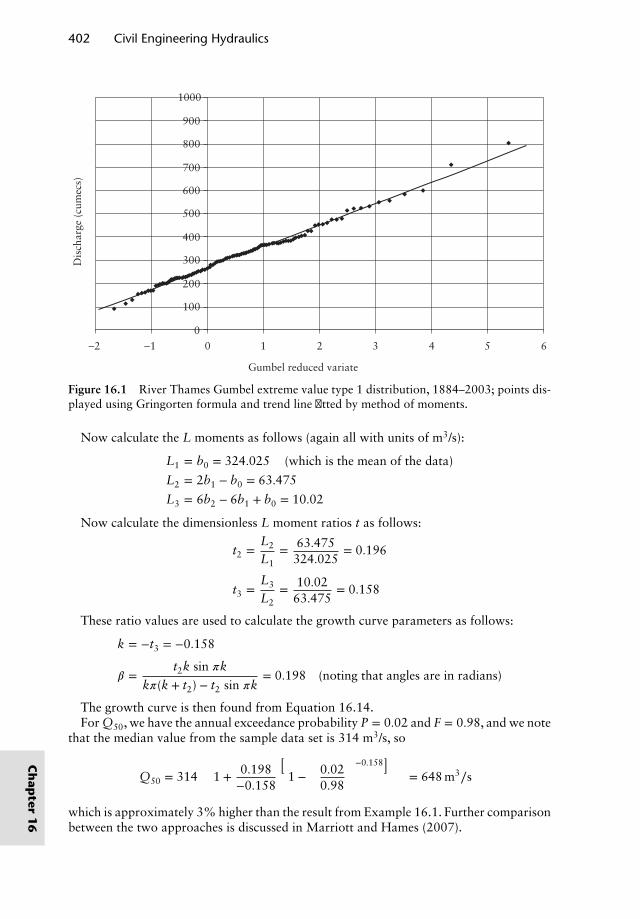
402 Civil Engineering Hydraulics
0
100
200
300
400
500
600
700
800
900
1000
−2 −1 0 1 2 3 4 5 6
Gumbel reduced variate
Dis
char
ge (
cum
ecs)
Figure 16.1 River Thames Gumbel extreme value type 1 distribution, 1884–2003; points dis-played using Gringorten formula and trend line fitted by method of moments.
Now calculate the L moments as follows (again all with units of m3/s):
L1 = b0 = 324.025 (which is the mean of the data)
L2 = 2b1 − b0 = 63.475
L3 = 6b2 − 6b1 + b0 = 10.02
Now calculate the dimensionless L moment ratios t as follows:
t2 =L2
L1= 63.475
324.025= 0.196
t3 =L3
L2= 10.02
63.475= 0.158
These ratio values are used to calculate the growth curve parameters as follows:
k = −t3 = −0.158
𝛽 =t2k sin 𝜋k
k𝜋(k + t2) − t2 sin 𝜋k= 0.198 (noting that angles are in radians)
The growth curve is then found from Equation 16.14.For Q50, we have the annual exceedance probability P = 0.02 and F = 0.98, and we note
that the median value from the sample data set is 314 m3/s, so
Q50 = 314
{1 + 0.198
−0.158
[1 −
(0.020.98
)−0.158]}
= 648 m3∕s
which is approximately 3% higher than the result from Example 16.1. Further comparisonbetween the two approaches is discussed in Marriott and Hames (2007).
Ch
apter
16
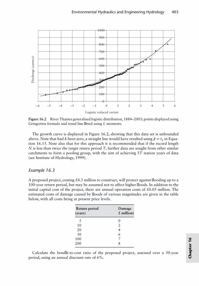
Environmental Hydraulics and Engineering Hydrology 403
0
100
200
300
400
500
600
700
800
900
1000
−6 −5 −4 −3 −2 −1 0 1 2 3 4 5 6
Logistic reduced variate
Dis
char
ge (
cum
ecs)
Figure 16.2 River Thames generalised logistic distribution, 1884–2003; points displayed usingGringorten formula and trend line fitted using L moments.
The growth curve is displayed in Figure 16.2, showing that this data set is unboundedabove. Note that had k been zero, a straight line would have resulted using 𝛽 = t2 in Equa-tion 16.15. Note also that for this approach it is recommended that if the record lengthN is less than twice the target return period T, further data are sought from other similarcatchments to form a pooling group, with the aim of achieving 5T station years of data(see Institute of Hydrology, 1999).
Example 16.3
A proposed project, costing £4.5 million to construct, will protect against flooding up to a100-year return period, but may be assumed not to affect higher floods. In addition to theinitial capital cost of the project, there are annual operation costs of £0.05 million. Theestimated costs of damage caused by floods of various magnitudes are given in the tablebelow, with all costs being at present price levels.
Return period Damage(years) £ million)
5 010 220 450 6
100 7200 8
Calculate the benefit-to-cost ratio of the proposed project, assessed over a 50-yearperiod, using an annual discount rate of 6%. Ch
apte
r1
6
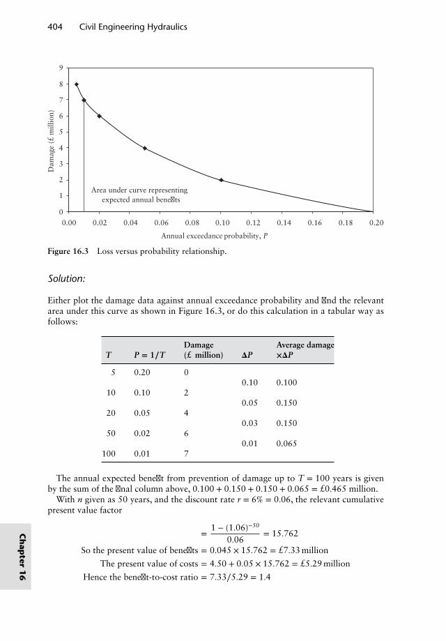
404 Civil Engineering Hydraulics
Area under curve representingexpected annual benefits
0
1
2
3
4
5
6
7
8
9
0.00 0.02 0.04 0.06 0.08 0.10 0.12 0.14 0.16 0.18 0.20
Annual exceedance probability, P
Dam
age
(£ m
illio
n)
Figure 16.3 Loss versus probability relationship.
Solution:
Either plot the damage data against annual exceedance probability and find the relevantarea under this curve as shown in Figure 16.3, or do this calculation in a tabular way asfollows:
Damage Average damageT P = 1∕T (£ million) 𝚫P ×𝚫P
5 0.20 00.10 0.100
10 0.10 20.05 0.150
20 0.05 40.03 0.150
50 0.02 60.01 0.065
100 0.01 7
The annual expected benefit from prevention of damage up to T = 100 years is givenby the sum of the final column above, 0.100 + 0.150 + 0.150 + 0.065 = £0.465 million.
With n given as 50 years, and the discount rate r = 6% = 0.06, the relevant cumulativepresent value factor
= 1 − (1.06)−50
0.06= 15.762
So the present value of benefits = 0.045 × 15.762 = £7.33 million
The present value of costs = 4.50 + 0.05 × 15.762 = £5.29 million
Hence the benefit-to-cost ratio = 7.33∕5.29 = 1.4
Ch
apter
16
Environmental Hydraulics and Engineering Hydrology 405
Taking a vertical cut-off line at P = 0.01 in Figure 16.3 is consistent with the instructionto assume that the proposed works will not affect rarer floods, but it is likely not to becompletely realistic. If the project will have some beneficial impact on higher return periodfloods, the value presented above may be regarded as a lower bound to the true benefit-to-cost ratio. With further data, the vertical line could be replaced by a more realistic post-project loss against probability curve, to evaluate what are referred to as above-design-standard benefits (Penning-Rowsell and Green, 2000).
References and recommended reading
Butler, D. and Davies, J. W. (2011) Urban Drainage, 3rd edn, Spon, Abingdon, UK.Chadwick, A., Morfett, J. and Borthwick, M. (2013) Hydraulics in Civil and Environmental
Engineering, 5th edn, Taylor & Francis, Abingdon, UK.Fenner, R. A., Ainger, C. M., Cruickshank, H. J. and Guthrie, P. M. (2006) Widening engi-
neering horizons: addressing the complexity of sustainable development, Proceedings of theInstitution of Civil Engineers Engineering Sustainability, 159, ES4 December, 145–154.
Fleming, G. (Ed) (2002) Flood Risk Management, Learning to Live with Rivers, ThomasTelford, London.
Gringorten, I. I. (1963) A plotting rule for extreme probability paper, Journal of GeophysicalResearch, 68, 813–814.
Herschy, R. (2003) World Catalogue of Maximum Observed Floods, IAHS Publication,Wallingford, UK.
Herschy, R. (2004) World Catalogue of Maximum Observed Floods (Errata and SupplementaryData), IAHS Publication, Wallingford, UK.
Institute of Hydrology (1999) Flood Estimation Handbook, Institute of Hydrology, now theCentre for Ecology and Hydrology, Wallingford, UK.
Knight, D. W. and Shamsheldin, A. Y. (Eds) (2006) River Basin Modelling for Flood Risk Miti-gation, Taylor & Francis, London.
Loveless, J. H., Sellin, R. H. J., Bryant, T. B., Wormleaton, P. R., Catmur, S. and Hey, R. (2000)The effect of overbank flow in a meandering river on its conveyance and the transport ofgraded sediments, Journal of the Chartered Institution of Water and Environmental Man-agement, 14, 447–455.
Mansell, M. G. (2003) Rural and Urban Hydrology, Thomas Telford, London.Marriott, M. J. and Hames, D. P. (2007) Comparison of reduced variates for flood frequency
estimation from gauged river flow records, Second IMA International Conference on FloodRisk Assessment, The Institute of Mathematics and its Applications, Plymouth, UK.
Marsh, T. J., Greenfield, B. J. and Hannaford, J. A. (2005) The 1894 Thames flood – a reap-praisal, Proceedings of the Institution of Civil Engineers Water Management, 158, WM3September, 103–110.
McGahey, C., Samuels, P. G., Knight, D. W. and O’Hare, M. T. (2008) Estimating river flowcapacity in practice, Journal of Flood Risk Management, 1, 1, 23–33.
Penning-Rowsell, E. C. and Green, C. (2000) New insights into the appraisal of flood-alleviationbenefits: (1) Flood damage and flood loss information, and (2) the broader context, Journalof the Chartered Institution of Water and Environmental Management, 14, 347–362.
Shaw, E. M., Beven, K. J., Chappell, N. A. and Lamb, R. (2011) Hydrology in Practice, 4th edn,Taylor & Francis, Abingdon, UK.
Tebbut, T. H. Y. (1998) Principles of Water Quality Control, 5th edn, Butterworth-Heinemann,Oxford, UK.
Water UK/WRc (2012) Sewers for Adoption – A Design and Construction Guide for Develop-ers, 7th edn, WRc, Swindon, UK. C
hap
ter
16
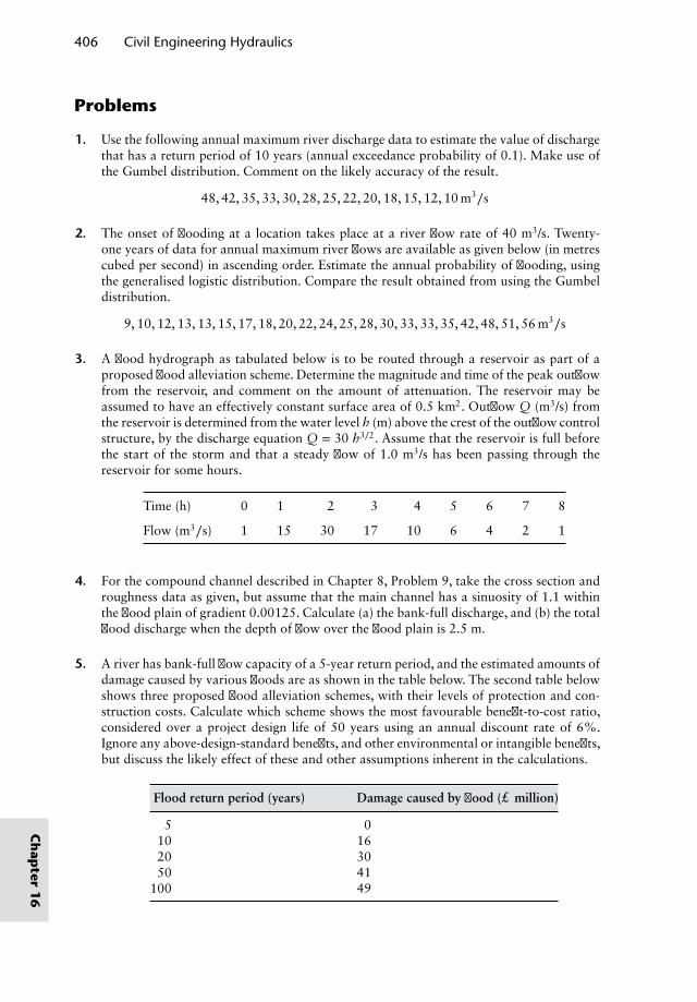
406 Civil Engineering Hydraulics
Problems
1. Use the following annual maximum river discharge data to estimate the value of dischargethat has a return period of 10 years (annual exceedance probability of 0.1). Make use ofthe Gumbel distribution. Comment on the likely accuracy of the result.
48, 42, 35, 33, 30, 28, 25, 22, 20, 18, 15, 12, 10 m3∕s
2. The onset of flooding at a location takes place at a river flow rate of 40 m3/s. Twenty-one years of data for annual maximum river flows are available as given below (in metrescubed per second) in ascending order. Estimate the annual probability of flooding, usingthe generalised logistic distribution. Compare the result obtained from using the Gumbeldistribution.
9, 10, 12, 13, 13, 15, 17, 18, 20, 22, 24, 25, 28, 30, 33, 33, 35, 42, 48, 51, 56 m3∕s
3. A flood hydrograph as tabulated below is to be routed through a reservoir as part of aproposed flood alleviation scheme. Determine the magnitude and time of the peak outflowfrom the reservoir, and comment on the amount of attenuation. The reservoir may beassumed to have an effectively constant surface area of 0.5 km2. Outflow Q (m3/s) fromthe reservoir is determined from the water level h (m) above the crest of the outflow controlstructure, by the discharge equation Q = 30 h3∕2. Assume that the reservoir is full beforethe start of the storm and that a steady flow of 1.0 m3/s has been passing through thereservoir for some hours.
Time (h) 0 1 2 3 4 5 6 7 8
Flow (m3∕s) 1 15 30 17 10 6 4 2 1
4. For the compound channel described in Chapter 8, Problem 9, take the cross section androughness data as given, but assume that the main channel has a sinuosity of 1.1 withinthe flood plain of gradient 0.00125. Calculate (a) the bank-full discharge, and (b) the totalflood discharge when the depth of flow over the flood plain is 2.5 m.
5. A river has bank-full flow capacity of a 5-year return period, and the estimated amounts ofdamage caused by various floods are as shown in the table below. The second table belowshows three proposed flood alleviation schemes, with their levels of protection and con-struction costs. Calculate which scheme shows the most favourable benefit-to-cost ratio,considered over a project design life of 50 years using an annual discount rate of 6%.Ignore any above-design-standard benefits, and other environmental or intangible benefits,but discuss the likely effect of these and other assumptions inherent in the calculations.
Flood return period (years) Damage caused by flood (£ million)
5 010 1620 3050 41
100 49
Ch
apter
16

Environmental Hydraulics and Engineering Hydrology 407
Level of protection, expressed Construction costScheme as a return period (years) (£ million)
A 20 16B 50 22C 100 28
Ch
apte
r1
6

Chapter 17Introduction to CoastalEngineering
17.1 Introduction
This chapter provides an introduction to theory that underpins coastal engineering, anextremely wide-ranging specialism with major challenges to design coastal structures andmanage shorelines. Starting with waves and wave theories, the text leads through waveprocesses and properties, tides, surges and mean sea level including a section on tsunamiwaves. Worked examples are included, with references for further study, as well as addi-tional problems to tackle.
17.2 Waves and wave theories
Coastal waves are mainly generated by the action of wind blowing across the sea surface.This causes the surface of the sea to exert a frictional drag on the lower layer of the wind,with the top layer (with the least drag) moving faster than the lower layer. This sets up acircular motion of wind energy that acts on the sea and thus creates waves. These wavestravel vast differences in various directions, reducing gradually in height in the absenceof further winds, generally only stopping when they meet an obstacle such as land or acoastal structure. Figure 17.1 illustrates two wave types in general: (a) regular long-crestedwaves following a sinusoidal pattern, and (b) random short-crested waves consisting of anumber of sinusoidal waves travelling in different directions superimposed on top of eachother. In general long-crested waves (see also Section 17.2.1) are observed in the nearshoreregion, whereas random short-crested waves (also see Section 17.2.4) are more commonlyobserved offshore.
In general, there are two types of wave theories: linear wave theory, sometimes knownas Airy’s waves, is the earliest, simplest and most widely used by coastal engineers; and,secondly, non-linear wave theory (e.g. Cnoidal and Stokes waves) is more complex andgives accurate predictions in shallow waters.
Nalluri & Featherstone’s Civil Engineering Hydraulics: Essential Theory with Worked Examples,Sixth Edition. Martin Marriott.© 2016 John Wiley & Sons, Ltd. Published 2016 by John Wiley & Sons, Ltd.Companion Website: www.wiley.com/go/Marriott
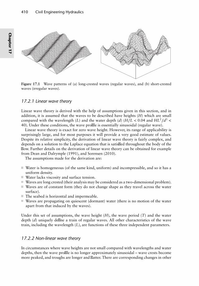
410 Civil Engineering Hydraulics
Figure 17.1 Wave patterns of (a) long-crested waves (regular waves), and (b) short-crestedwaves (irregular waves).
17.2.1 Linear wave theory
Linear wave theory is derived with the help of assumptions given in this section, and inaddition, it is assumed that the waves to be described have heights (H) which are smallcompared with the wavelength (L) and the water depth (d) (H∕L < 0.04 and HL2∕d3 <
40). Under these conditions, the wave profile is essentially sinusoidal (regular wave).Linear wave theory is exact for zero wave height. However, its range of applicability is
surprisingly large, and for most purposes it will provide a very good estimate of values.Despite its relative simplicity, the derivation of linear wave theory is fairly complex, anddepends on a solution to the Laplace equation that is satisfied throughout the body of theflow. Further details on the derivation of linear wave theory can be obtained for examplefrom Dean and Dalrymple (1991), and Sorensen (2010).
The assumptions made for the derivation are:
Water is homogeneous (of the same kind, uniform) and incompressible, and so it has auniform density.Water lacks viscosity and surface tension.Waves are long crested (their analysis may be considered as a two-dimensional problem).Waves are of constant form (they do not change shape as they travel across the watersurface).The seabed is horizontal and impermeable.Waves are propagating on quiescent (dormant) water (there is no motion of the waterapart from that induced by the waves).
Under this set of assumptions, the wave height (H), the wave period (T) and the waterdepth (d) uniquely define a train of regular waves. All other characteristics of the wavetrain, including the wavelength (L), are functions of these three independent parameters.
17.2.2 Non-linear wave theory
In circumstances where wave heights are not small compared with wavelengths and waterdepths, then the wave profile is no longer approximately sinusoidal – wave crests becomemore peaked, and troughs are longer and flatter. There are corresponding changes in other
Ch
apter
17
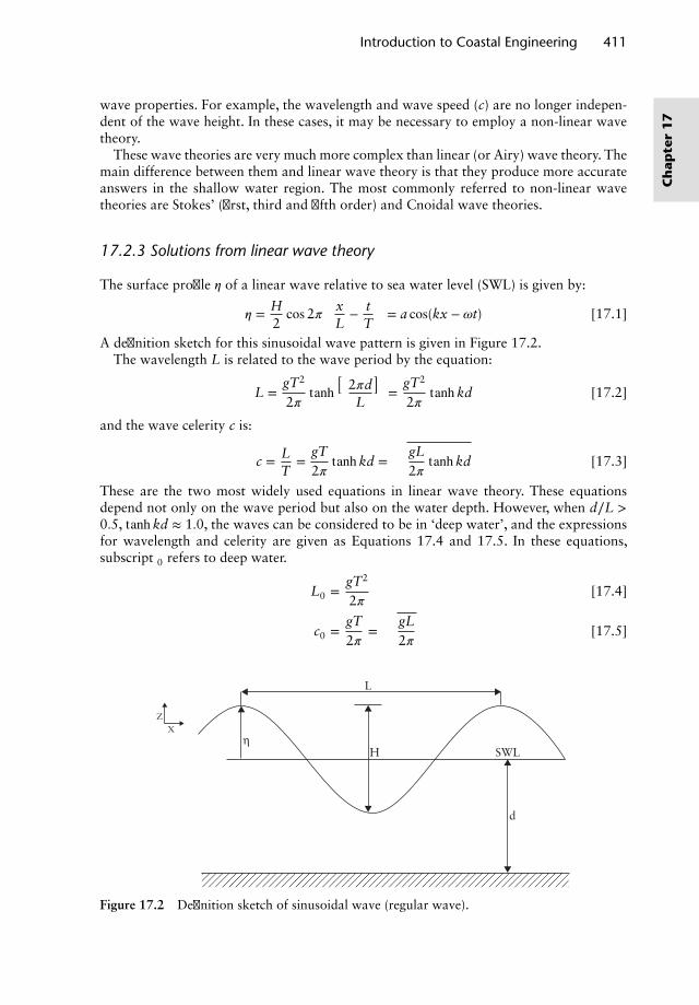
Introduction to Coastal Engineering 411
wave properties. For example, the wavelength and wave speed (c) are no longer indepen-dent of the wave height. In these cases, it may be necessary to employ a non-linear wavetheory.
These wave theories are very much more complex than linear (or Airy) wave theory. Themain difference between them and linear wave theory is that they produce more accurateanswers in the shallow water region. The most commonly referred to non-linear wavetheories are Stokes’ (first, third and fifth order) and Cnoidal wave theories.
17.2.3 Solutions from linear wave theory
The surface profile 𝜂 of a linear wave relative to sea water level (SWL) is given by:
𝜂 = H2cos2𝜋
( xL
− tT
)= a cos(kx − 𝜔t) [17.1]
A definition sketch for this sinusoidal wave pattern is given in Figure 17.2.The wavelength L is related to the wave period by the equation:
L =gT2
2𝜋tanh
(2𝜋dL
)=
gT2
2𝜋tanh kd [17.2]
and the wave celerity c is:
c = LT
=gT2𝜋
tanh kd =√
gL2𝜋
tanh kd [17.3]
These are the two most widely used equations in linear wave theory. These equationsdepend not only on the wave period but also on the water depth. However, when d∕L >
0.5, tanh kd ≈ 1.0, the waves can be considered to be in ‘deep water’, and the expressionsfor wavelength and celerity are given as Equations 17.4 and 17.5. In these equations,subscript 0 refers to deep water.
L0 =gT2
2𝜋[17.4]
c0 =gT2𝜋
=√
gL2𝜋
[17.5]
L
SWL
d
Z
Xη
H
Figure 17.2 Definition sketch of sinusoidal wave (regular wave).
Ch
apte
r1
7
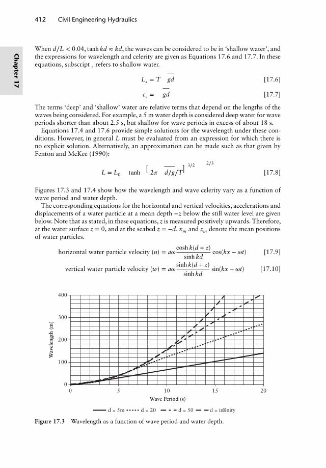
412 Civil Engineering Hydraulics
When d∕L < 0.04, tanh kd ≈ kd, the waves can be considered to be in ‘shallow water’, andthe expressions for wavelength and celerity are given as Equations 17.6 and 17.7. In theseequations, subscript s refers to shallow water.
Ls = T√
gd [17.6]
cs =√
gd [17.7]
The terms ‘deep’ and ‘shallow’ water are relative terms that depend on the lengths of thewaves being considered. For example, a 5 m water depth is considered deep water for waveperiods shorter than about 2.5 s, but shallow for wave periods in excess of about 18 s.
Equations 17.4 and 17.6 provide simple solutions for the wavelength under these con-ditions. However, in general L must be evaluated from an expression for which there isno explicit solution. Alternatively, an approximation can be made such as that given byFenton and McKee (1990):
L = L0
{tanh
[(2𝜋√
d∕g∕T)3∕2
]}2∕3
[17.8]
Figures 17.3 and 17.4 show how the wavelength and wave celerity vary as a function ofwave period and water depth.
The corresponding equations for the horizontal and vertical velocities, accelerations anddisplacements of a water particle at a mean depth −z below the still water level are givenbelow. Note that as stated, in these equations, z is measured positively upwards. Therefore,at the water surface z = 0, and at the seabed z = −d. xm and zm denote the mean positionsof water particles.
horizontal water particle velocity (u) = a𝜔cosh k(d + z)
sinhkdcos(kx − 𝜔t) [17.9]
vertical water particle velocity (w) = a𝜔sinhk(d + z)
sinh kdsin(kx − 𝜔t) [17.10]
Wave Period (s)
Wav
elen
gth
(m)
400
300
200
100
0
d = 5m d = 20 d = 50 d = infinity
0 5 10 15 20
Figure 17.3 Wavelength as a function of wave period and water depth.
Ch
apter
17
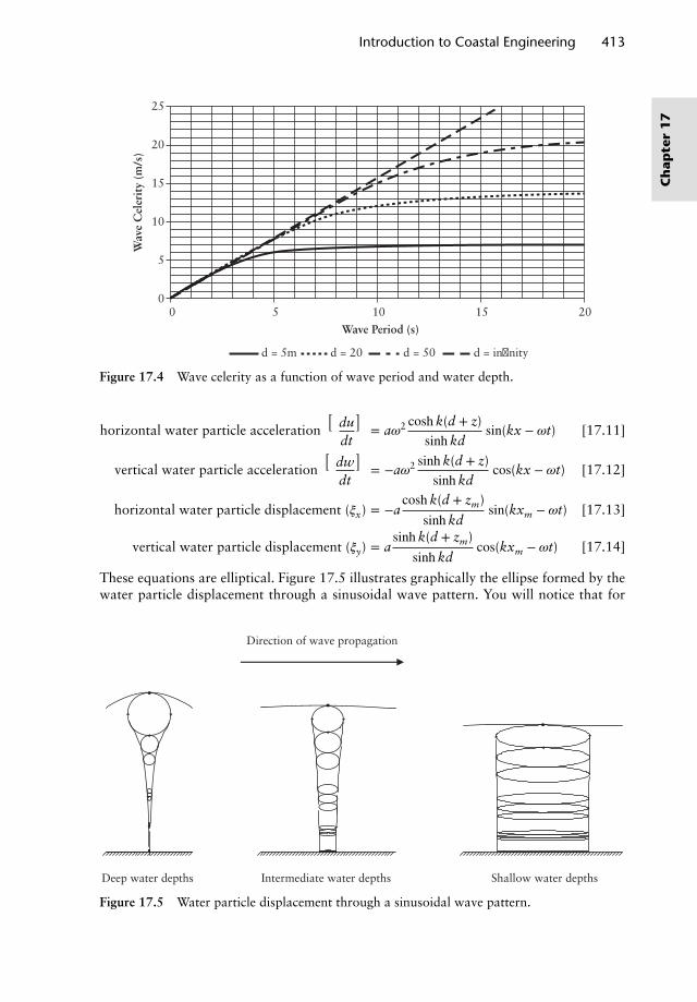
Introduction to Coastal Engineering 413
Wave Period (s)
0 5 10 15 20
d = 5m d = 20 d = 50 d = infinity
Wav
e C
eler
ity
(m/s
)
25
20
15
10
5
0
Figure 17.4 Wave celerity as a function of wave period and water depth.
horizontal water particle acceleration(
dudt
)= a𝜔2 cosh k(d + z)
sinh kdsin(kx − 𝜔t) [17.11]
vertical water particle acceleration(
dwdt
)= −a𝜔2 sinhk(d + z)
sinh kdcos(kx − 𝜔t) [17.12]
horizontal water particle displacement (𝜉x) = −acosh k(d + zm)
sinhkdsin(kxm − 𝜔t) [17.13]
vertical water particle displacement (𝜉y) = asinhk(d + zm)
sinh kdcos(kxm − 𝜔t) [17.14]
These equations are elliptical. Figure 17.5 illustrates graphically the ellipse formed by thewater particle displacement through a sinusoidal wave pattern. You will notice that for
Direction of wave propagation
Deep water depths Intermediate water depths Shallow water depths
Figure 17.5 Water particle displacement through a sinusoidal wave pattern.
Ch
apte
r1
7
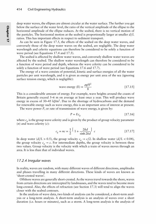
414 Civil Engineering Hydraulics
deep water waves, the ellipses are almost circular at the water surface. The further you getbelow the surface of the water level, the ratio of the vertical amplitude of the ellipse to thehorizontal amplitude of the ellipse reduces. At the seabed, there is no vertical motion ofthe particles. The horizontal motion at the seabed is proportionally larger at smaller d∕Lratios. This has important effects in respect to sediment transport.
As can be seen in Figure 17.5, the effects of the seabed on the deep water waves, andconversely those of the deep water waves on the seabed, are negligible. The deep waterwavelength and celerity equations can therefore be considered to be solely a function ofwave period (see Equations 17.4 and 17.5).
The seabed is affected by shallow water waves, and conversely shallow water waves areaffected by the seabed. The shallow water wavelength can therefore be considered to bea function of wave period and depth, whereas the wave celerity can be considered to besolely a function of wave period (see Equations 17.6 and 17.7).
The energy of a wave consists of potential, kinetic and surface energies of all the waterparticles per unit wavelength, and it is given as energy per unit area of the sea (ignoringsurface tension energy, which is negligible):
wave energy (E) =𝜌gH2
8[17.15]
This is a considerable amount of energy. For example, wave heights around the coasts ofBritain generally exceed 5–6 m on average at least once a year. This will produce waveenergy in excess of 30–45 kJ/m2. Due to the shortage of hydrocarbons and the demandfor renewable energy such as wave energy, this is an important area of interest at present.
The wave power P, or rate of transmission of wave energy, is given by:
P = Ecg [17.16]
where cg is the group wave celerity and is given by the product of group velocity parameter(n) and wave celerity (c):
cg = nc = 12
(1 + 2kd
sinh2kd
)c [17.17]
In deep water (d∕L > 0.5), the group velocity cg → c∕2. In shallow water (d∕L < 0.04),the group velocity cg → c. For intermediate depths, the group velocity is between thesetwo values. Group velocity is the velocity with which a train of waves moves through anarea. It is less than that of individual waves.
17.2.4 Irregular waves
In reality, waves are random, with many different waves of different directions, amplitudesand phases travelling in many different directions. These kinds of waves are known as‘short-crested waves’.
Offshore waves are generally short-crested. As the waves travel towards the shore, wavesfrom certain directions are intercepted by landmasses, and the waves tend to become morelong-crested. Also, the effects of refraction (see Section 17.3) will tend to align the wavescloser with the seabed contours.
In the analysis of wave data, two kinds of analysis can be considered, a short-term anal-ysis or a long-term analysis. A short-term analysis is an analysis of waves over a shortduration (i.e. hours or minutes), such as a storm. A long-term analysis is the analysis of
Ch
apter
17
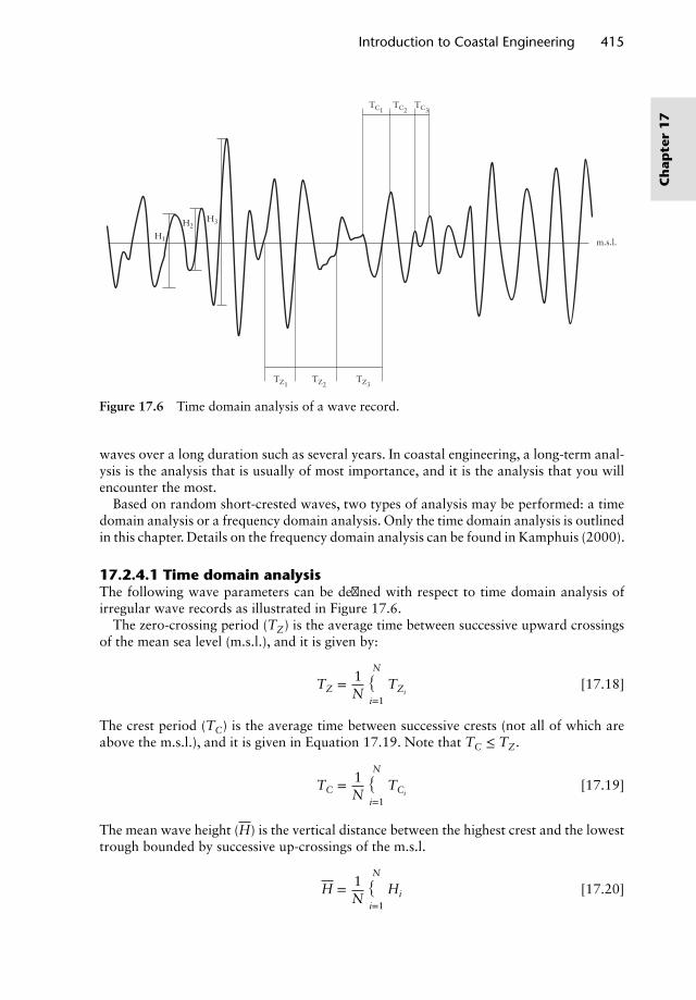
Introduction to Coastal Engineering 415
TC1
TZ1
H1
H2H3
TZ2TZ3
m.s.l.
TC2TC3
Figure 17.6 Time domain analysis of a wave record.
waves over a long duration such as several years. In coastal engineering, a long-term anal-ysis is the analysis that is usually of most importance, and it is the analysis that you willencounter the most.
Based on random short-crested waves, two types of analysis may be performed: a timedomain analysis or a frequency domain analysis. Only the time domain analysis is outlinedin this chapter. Details on the frequency domain analysis can be found in Kamphuis (2000).
17.2.4.1 Time domain analysisThe following wave parameters can be defined with respect to time domain analysis ofirregular wave records as illustrated in Figure 17.6.
The zero-crossing period (TZ) is the average time between successive upward crossingsof the mean sea level (m.s.l.), and it is given by:
TZ = 1N
N∑i=1
TZi[17.18]
The crest period (TC) is the average time between successive crests (not all of which areabove the m.s.l.), and it is given in Equation 17.19. Note that TC ≤ TZ.
TC = 1N
N∑i=1
TCi[17.19]
The mean wave height (H) is the vertical distance between the highest crest and the lowesttrough bounded by successive up-crossings of the m.s.l.
H = 1N
N∑i=1
Hi [17.20]
Ch
apte
r1
7
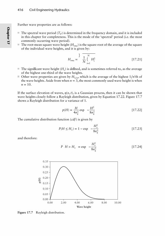
416 Civil Engineering Hydraulics
Further wave properties are as follows:
The spectral wave period (TP) is determined in the frequency domain, and it is includedin this chapter for completeness. This is the mode of the ‘spectral’ period (i.e. the mostcommonly occurring wave period).The root-mean square wave height (Hrms) is the square root of the average of the squareof the individual wave heights, and it is given by:
Hrms =
√√√√ 1N
N∑i=1
H2i [17.21]
The significant wave height (Hs) is defined, and is sometimes referred to, as the averageof the highest one-third of the wave heights.Other wave properties are given by H1∕n, which is the average of the highest 1∕n’th ofthe wave heights. Aside from when n = 3, the most commonly used wave height is whenn = 10.
If the surface elevation of waves, 𝜂(x, t), is a Gaussian process, then it can be shown thatwave heights closely follow a Rayleigh distribution, given by Equation 17.22. Figure 17.7shows a Rayleigh distribution for a variance of 1.
p(H) = H4𝜎2
𝜂
exp
[− H2
8𝜎2𝜂
][17.22]
The cumulative distribution function (cdf ) is given by
P(H ≤ H∗) = 1 − exp
[−
H2∗
8𝜎2𝜂
][17.23]
and therefore:
P(H > H∗
)= exp
[−
H2∗
8𝜎2𝜂
][17.24]
p(H
)
0.35
0.30
0.25
0.20
0.15
0.10
0.05
0.000.00 2.00 4.00
Wave height
6.00 8.00 10.00
Figure 17.7 Rayleigh distribution.
Ch
apter
17
Introduction to Coastal Engineering 417
From Equation 17.22, the following properties for random waves can be determined:
H =
∞
∫0
H p(H)dH = 2.51𝜎𝜂 [17.25]
Hrms =
√√√√√∞
∫0
H2p (H)dH = 2√
2𝜎𝜂 [17.26]
From Equation 17.26, therefore, Equation 17.24 may be rewritten as:
P(H > H∗
)= exp
[−(
H∗
Hrms
)2]
[17.27]
The average height of the highest 1∕n’th of the waves may be found by considering theheight H∗ above which the highest 1∕n’th of the waves lie, given by:
P(H > H∗
)=
∞
∫H∗
p (H)dH = 1n
[17.28]
Therefore, H1∕n may be written:
H1∕n =
∞∫H∗
Hp (H)dH
∞∫H∗
p (H)dH
= n
∞
∫H∗
Hp (H)dH [17.29]
Equating Equations 17.27 and 17.28 gives
H∗
Hrms=√lnn [17.30]
Using these relationships, it can be shown that:
H1∕3 = 1.416Hrms = 1.60H = 4.0𝜎𝜂 [17.31]
H1∕10 = 1.800Hrms = 2.03H [17.32]
H1∕100 = 2.359Hrms = 2.66H [17.33]
If m waves out of a total of N waves are larger than H∗, then:
P(H > H∗
)= exp
[−(
H∗
Hrms
)2]= m
N[17.34]
Therefore,
H∗
Hrms=√
− ln(m
N
)[17.35]
This is the same as Equation 17.30, since m∕N = 1∕n.
Ch
apte
r1
7
418 Civil Engineering Hydraulics
Putting n = 1 into Equation 17.35 gives Hmax, the wave height expected to be exceededonly once in a sample of N waves. Therefore, Hmax can be written as:
Hmax = Hrms
√lnN = Hs
√( lnN2
)[17.36]
Therefore, for a 20-minute wave trace of waves with a mean zero-crossing period of 7 s,the maximum wave height that could be expected in that period would be about 1.6 Hs.
17.2.4.2 Wave prediction from wind recordsFor a given wind speed, the waves produced will depend on the duration of the windD and the fetch F. The bigger the fetch or the longer the duration, the bigger the wavesproduced. However, as the wind contains only a limited amount of energy, there is a limitto the height of waves produced for a given duration and/or fetch. This is the point wherethe rate of transfer of energy to the waves equals the energy dissipation by wave breakingand friction.
Wind is recorded for meteorological purposes at many sites. This and the fact that wavemeasurement can be very difficult for several reasons, including the frequent inaccessibilityof the recording apparatus and maintenance problems, mean that wind speeds are oftenmore frequently recorded than waves. As storm waves are dependent solely on wind, dura-tion and fetch length, the most common technique used to determine the wave climate isusing wind records. This technique is commonly referred to as ‘hindcasting’.
17.2.4.3 Pierson Moskowitz wave spectrumThe most common technique used to determine wind speeds offshore is by means of thePierson Moskowitz spectrum (PMS). For a fully arisen sea, this is given as:
S(f , 𝜃)=
𝛼g2
(2𝜋)4 f 5exp
{−5
4
(fm
f
)4}
[17.37]
The PMS was derived from measurements of ocean waves taken by weather ships in theNorth Atlantic. It does not describe conditions in fetch-limited seas. It is not going to beconsidered any further in this chapter.
17.2.4.4 JONSWAP wave spectrumThe JONSWAP (Joint North Sea Wave Project) spectrum was derived for fetch-limitedseas. This spectrum was determined based on observations of wave heights in the NorthSea. It is more complicated than the equation for the PMS, because it is a function ofboth wind and fetch. This is the spectrum that is used for locally generated seas across(for example) estuaries. This is also the spectrum most likely to be encountered in coastalengineering.
The JONSWAP spectrum (Hasselmann et al., 1973) is given by the formula:
S(f , 𝜃)=
𝛼g2
(2𝜋)4 f 5exp
{−5
4
(fm
f
)4}𝛾a [17.38]
The PMS and JONSWAP spectra are deep water spectra. Where a spectrum is requiredin transitional water depths, the TMA spectrum may be used, which is given in Sec-tion 17.2.4.5; this is a modified JONSWAP spectrum.
Ch
apter
17
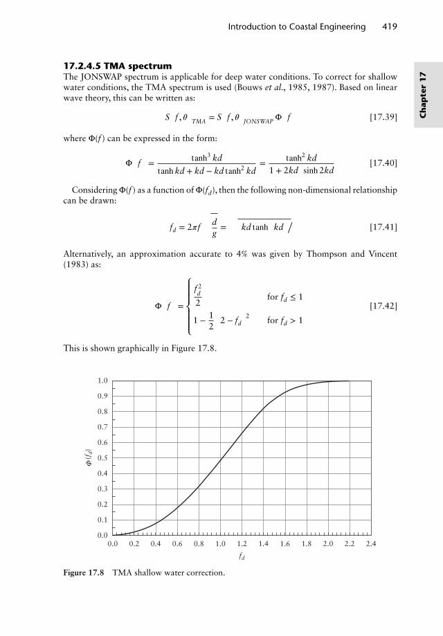
Introduction to Coastal Engineering 419
17.2.4.5 TMA spectrumThe JONSWAP spectrum is applicable for deep water conditions. To correct for shallowwater conditions, the TMA spectrum is used (Bouws et al., 1985, 1987). Based on linearwave theory, this can be written as:
S(f , 𝜃)
TMA = S(f , 𝜃)
JONSWAP Φ(f)
[17.39]
where Φ(f ) can be expressed in the form:
Φ(f)= tanh3 kd
tanh kd + kd − kd tanh2 kd= tanh2 kd
1 + 2kd/sinh2kd
[17.40]
Considering Φ(f ) as a function of Φ(fd), then the following non-dimensional relationshipcan be drawn:
fd = 2𝜋f
√dg=√[
kd tanh(kd)]
[17.41]
Alternatively, an approximation accurate to 4% was given by Thompson and Vincent(1983) as:
Φ(f)=
⎧⎪⎪⎨⎪⎪⎩
f 2d
2for fd ≤ 1
1 − 12
(2 − fd
)2for fd > 1
[17.42]
This is shown graphically in Figure 17.8.
1.0
0.9
0.8
0.7
0.6
0.5
0.4
0.3
0.2
0.1
1.0 1.2
fd
1.4 1.6 1.8 2.0 2.2 2.40.80.60.40.20.0
0.0
(fd)
Φ
Figure 17.8 TMA shallow water correction.
Ch
apte
r1
7
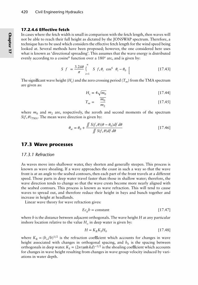
420 Civil Engineering Hydraulics
17.2.4.6 Effective fetchIn cases where the fetch width is small in comparison with the fetch length, then waves willnot be able to reach their full height as dictated by the JONSWAP spectrum. Therefore, atechnique has to be used which considers the effective fetch length for the wind speed beinglooked at. Several methods have been proposed; however, the one considered here useswhat is known as ‘directional spreading’. This assumes that the wave energy is distributedevenly according to a cosine6 function over a 180◦ arc, and is given by:
S(f)= 3.2𝛿𝜃
𝜋
n∑i=1
{S(f , 𝜃i
)cos6 (𝜃i − 𝜃0
)}[17.43]
The significant wave height (Hs) and the zero crossing period (Tm) from the TMA spectrumare given as:
Hs = 4√
m0 [17.44]
Tm =√
m0
m2[17.45]
where m0 and m2 are, respectively, the zeroth and second moments of the spectrumS(f , 𝜃)TMA. The mean wave direction is given by:
𝜃w = 𝜃0 +∬ S(f , 𝜃)(𝜃 − 𝜃0)df d𝜃
∬ S(f , 𝜃)df d𝜃[17.46]
17.3 Wave processes
17.3.1 Refraction
As waves move into shallower water, they shorten and generally steepen. This process isknown as wave shoaling. If a wave approaches the coast in such a way so that the wavefront is at an angle to the seabed contours, then each part of the front travels at a differentspeed. Those parts in deep water travel faster than those in shallow water; therefore, thewave direction tends to change so that the wave crests become more nearly aligned withthe seabed contours. This process is known as wave refraction. This will tend to causewaves to spread out, and therefore reduce their height in bays and bunch together andincrease in height at headlands.
Linear wave theory for wave refraction gives:
Ecgb = constant [17.47]
where b is the distance between adjacent orthogonals. The wave height H at any particularinshore location relative to the value Ho in deep water is given by:
H = KRKSH0 [17.48]
where KR = (bo∕b)1∕2 is the refraction coefficient which accounts for changes in waveheight associated with changes in orthogonal spacing, and b0 is the spacing betweenorthogonals in deep water. KS = (2n tanhkd)−1∕2 is the shoaling coefficient which accountsfor changes in wave height resulting from changes in wave group velocity induced by vari-ations in water depth.
Ch
apter
17
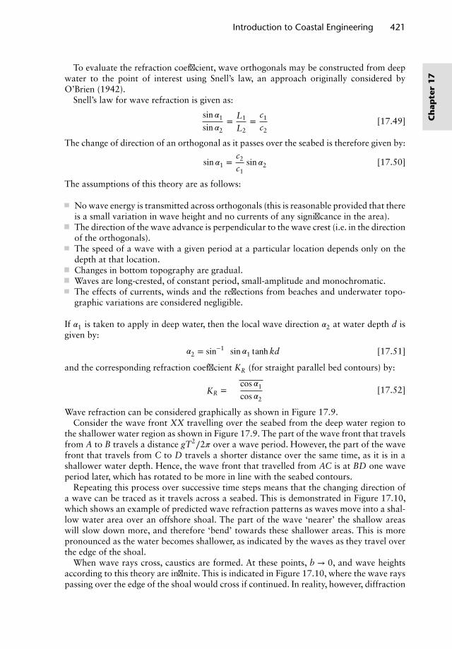
Introduction to Coastal Engineering 421
To evaluate the refraction coefficient, wave orthogonals may be constructed from deepwater to the point of interest using Snell’s law, an approach originally considered byO’Brien (1942).
Snell’s law for wave refraction is given as:
sin 𝛼1
sin 𝛼2= L1
L2=
c1
c2[17.49]
The change of direction of an orthogonal as it passes over the seabed is therefore given by:
sin 𝛼1 =c2
c1sin 𝛼2 [17.50]
The assumptions of this theory are as follows:
No wave energy is transmitted across orthogonals (this is reasonable provided that thereis a small variation in wave height and no currents of any significance in the area).The direction of the wave advance is perpendicular to the wave crest (i.e. in the directionof the orthogonals).The speed of a wave with a given period at a particular location depends only on thedepth at that location.Changes in bottom topography are gradual.Waves are long-crested, of constant period, small-amplitude and monochromatic.The effects of currents, winds and the reflections from beaches and underwater topo-graphic variations are considered negligible.
If 𝛼1 is taken to apply in deep water, then the local wave direction 𝛼2 at water depth d isgiven by:
𝛼2 = sin−1 (sin 𝛼1 tanh kd)
[17.51]
and the corresponding refraction coefficient KR (for straight parallel bed contours) by:
KR =√
cos 𝛼1
cos 𝛼2[17.52]
Wave refraction can be considered graphically as shown in Figure 17.9.Consider the wave front XX travelling over the seabed from the deep water region to
the shallower water region as shown in Figure 17.9. The part of the wave front that travelsfrom A to B travels a distance gT2∕2𝜋 over a wave period. However, the part of the wavefront that travels from C to D travels a shorter distance over the same time, as it is in ashallower water depth. Hence, the wave front that travelled from AC is at BD one waveperiod later, which has rotated to be more in line with the seabed contours.
Repeating this process over successive time steps means that the changing direction ofa wave can be traced as it travels across a seabed. This is demonstrated in Figure 17.10,which shows an example of predicted wave refraction patterns as waves move into a shal-low water area over an offshore shoal. The part of the wave ‘nearer’ the shallow areaswill slow down more, and therefore ‘bend’ towards these shallower areas. This is morepronounced as the water becomes shallower, as indicated by the waves as they travel overthe edge of the shoal.
When wave rays cross, caustics are formed. At these points, b → 0, and wave heightsaccording to this theory are infinite. This is indicated in Figure 17.10, where the wave rayspassing over the edge of the shoal would cross if continued. In reality, however, diffraction
Ch
apte
r1
7
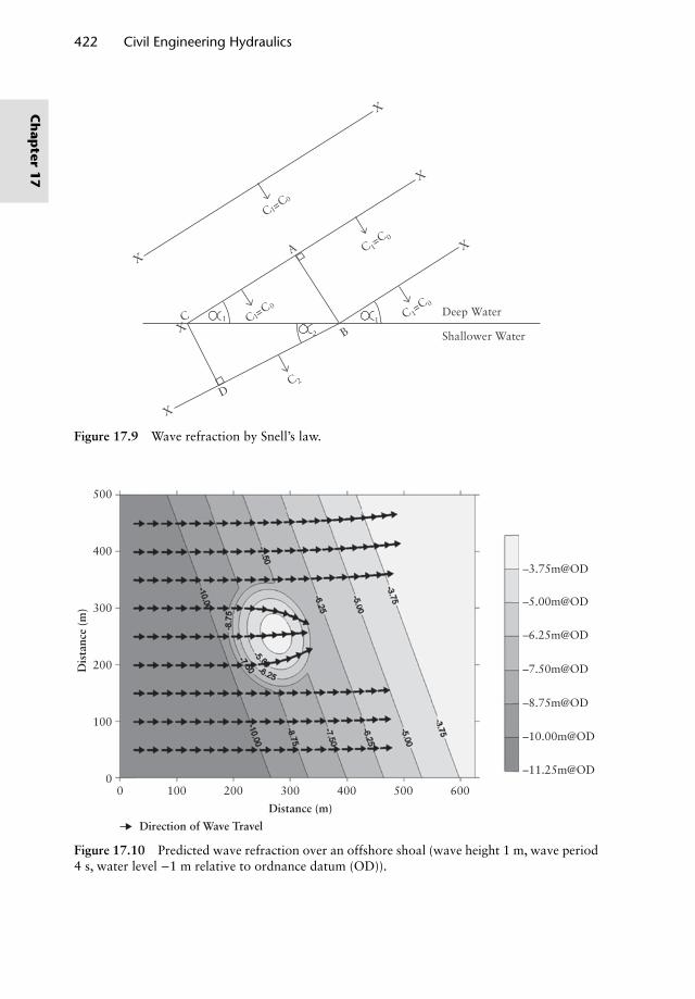
422 Civil Engineering Hydraulics
Deep Water
Shallower Water
X
XA
BC
D
X
X
X1
2
1C =C
C 2
1
0C 1
=C 0
C =C1
0
X
C 1=C 0
Figure 17.9 Wave refraction by Snell’s law.
500
400
300
200
100
00 100 200 300
Distance (m)
Dis
tanc
e (m
)
Direction of Wave Travel
400 500 600
–3.75m@OD
–5.00m@OD
–6.25m@OD
–7.50m@OD
–8.75m@OD
–10.00m@OD
–11.25m@OD
Figure 17.10 Predicted wave refraction over an offshore shoal (wave height 1 m, wave period4 s, water level −1 m relative to ordnance datum (OD)).
Ch
apter
17
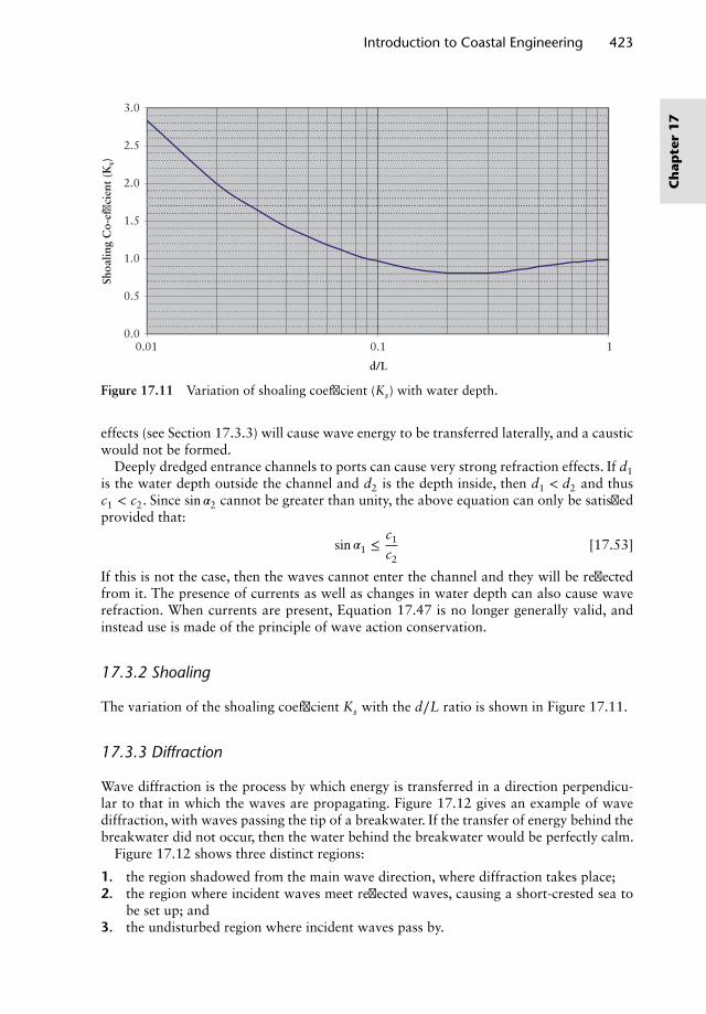
Introduction to Coastal Engineering 423
0.0
0.5
1.0
1.5
2.0
2.5
3.0
0.01 0.1 1
Shoa
ling
Co-
effic
ient
(K
s)
d/L
Figure 17.11 Variation of shoaling coefficient (Ks) with water depth.
effects (see Section 17.3.3) will cause wave energy to be transferred laterally, and a causticwould not be formed.
Deeply dredged entrance channels to ports can cause very strong refraction effects. If d1is the water depth outside the channel and d2 is the depth inside, then d1 < d2 and thusc1 < c2. Since sin 𝛼2 cannot be greater than unity, the above equation can only be satisfiedprovided that:
sin 𝛼1 ≤ c1
c2[17.53]
If this is not the case, then the waves cannot enter the channel and they will be reflectedfrom it. The presence of currents as well as changes in water depth can also cause waverefraction. When currents are present, Equation 17.47 is no longer generally valid, andinstead use is made of the principle of wave action conservation.
17.3.2 Shoaling
The variation of the shoaling coefficient Ks with the d∕L ratio is shown in Figure 17.11.
17.3.3 Diffraction
Wave diffraction is the process by which energy is transferred in a direction perpendicu-lar to that in which the waves are propagating. Figure 17.12 gives an example of wavediffraction, with waves passing the tip of a breakwater. If the transfer of energy behind thebreakwater did not occur, then the water behind the breakwater would be perfectly calm.
Figure 17.12 shows three distinct regions:
1. the region shadowed from the main wave direction, where diffraction takes place;2. the region where incident waves meet reflected waves, causing a short-crested sea to
be set up; and3. the undisturbed region where incident waves pass by.
Ch
apte
r1
7
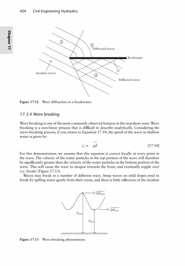
424 Civil Engineering Hydraulics
1
2
3
Diffracted waves
Breakwater
Reflected waves
Incident waves
Figure 17.12 Wave diffraction at a breakwater.
17.3.4 Wave breaking
Wave breaking is one of the most commonly observed features in the nearshore zone. Wavebreaking is a non-linear process that is difficult to describe analytically. Considering thewave-breaking process, if you return to Equation 17.54, the speed of the wave in shallowwater is given by:
cs =√
gd [17.54]
For this demonstration, we assume that this equation is correct locally at every point inthe wave. The velocity of the water particles in the top portion of the wave will thereforebe significantly greater than the velocity of the water particles in the bottom portion of thewave. This will cause the wave to steepen towards the front, and eventually topple over(i.e. break) (Figure 17.13).
Waves may break in a number of different ways. Steep waves on mild slopes tend tobreak by spilling water gently from their crests, and there is little reflection of the incident
dmin
dmax
gdmin
gdmax
Figure 17.13 Wave-breaking phenomenon.
Ch
apter
17
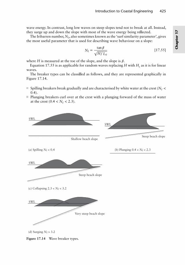
Introduction to Coastal Engineering 425
wave energy. In contrast, long low waves on steep slopes tend not to break at all. Instead,they surge up and down the slope with most of the wave energy being reflected.
The Iribarren number, NI, also sometimes known as the ‘surf similarity parameter’, givesthe most useful parameter that is used for describing wave behaviour on a slope:
NI =tan 𝛽√H∕L0
[17.55]
where H is measured at the toe of the slope, and the slope is 𝛽.Equation 17.55 is as applicable for random waves replacing H with Hs as it is for linear
waves.The breaker types can be classified as follows, and they are represented graphically in
Figure 17.14.
Spilling breakers break gradually and are characterised by white water at the crest (NI <
0.4).Plunging breakers curl over at the crest with a plunging forward of the mass of waterat the crest (0.4 < NI < 2.3).
SWL
SWL
SWL
SWL
Shallow beach slope
(a) Spilling NI < 0.4
(c) Collapsing 2.3 < NI < 3.2
(d) Surging NI > 3.2
(b) Plunging 0.4 < NI < 2.3
Steep beach slope
Very steep beach slope
Steep beach slope
Figure 17.14 Wave breaker types.
Ch
apte
r1
7
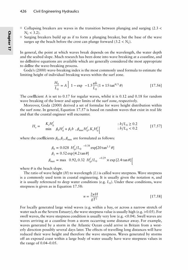
426 Civil Engineering Hydraulics
Collapsing breakers are waves in the transition between plunging and surging (2.3 <NI < 3.2).Surging breakers build up as if to form a plunging breaker, but the base of the wavesurges up the beach before the crest can plunge forward (3.2 < NI).
In general, the point at which waves break depends on the wavelength, the water depthand the seabed slope. Much research has been done into wave breaking at a coastline, andno definitive equations are available which are generally considered the most appropriateto define the wave-breaking process.
Goda’s (2000) wave-breaking index is the most commonly used formula to estimate thelimiting height of individual breaking waves within the surf zone.
Hb
L0= A
{1 − exp
[−1.5𝜋h
L0(1 + 15 tan4∕3 𝜃)
]}[17.56]
The coefficient A is set to 0.17 for regular waves, whilst it is 0.12 and 0.18 for randomwave breaking of the lower and upper limits of the surf zone, respectively.
Moreover, Goda (2000) derived a set of formulae for wave height distribution withinthe surf zone. In general, Equation 17.57 is based on random waves that exist in real lifeand that the coastal engineer will encounter.
Hs =
{KsH
∕0
min{(𝛽0H∕
0 + 𝛽1h), 𝛽maxH
∕0, KsH
∕0
} : h∕L0 ≥ 0.2: h∕L0 < 0.2
[17.57]
where the coefficients 𝛽0, 𝛽1, 𝛽max are formulated as follows:
𝛽0 = 0.028(H∕
0∕L0
)−0.38 exp[20 tan1.5 𝜃]
𝛽1 = 0.52 exp [4.2 tan 𝜃]
𝛽max = max{
0.92, 0.32(H∕
0∕L0
)−0.29 × exp [2.4 tan 𝜃]}
where 𝜃 is the beach slope.The ratio of wave height (H) to wavelength (L) is called wave steepness. Wave steepness
is a commonly used term in coastal engineering. It is usually given the notation n, andit is usually referenced to deep water conditions (e.g. L0). Under these conditions, wavesteepness is given as in Equation 17.58:
n = 2𝜋HgT2
[17.58]
For locally generated large wind waves (e.g. within a bay, or across a narrow stretch ofwater such as the Severn Estuary), the wave steepness value is usually high (e.g.>0.05). Forswell waves, the wave steepness condition is usually very low (e.g.<0.04). Swell waves arewaves arriving at a coastline from a storm occurring some distance away. For example,waves generated by a storm in the Atlantic Ocean could arrive in Britain from a west-erly direction possibly several days later. The effects of travelling long distances will havereduced their wave height and therefore the wave steepness. Waves generated by stormsoff an exposed coast within a large body of water usually have wave steepness values inthe range of 0.04–0.05.
Ch
apter
17
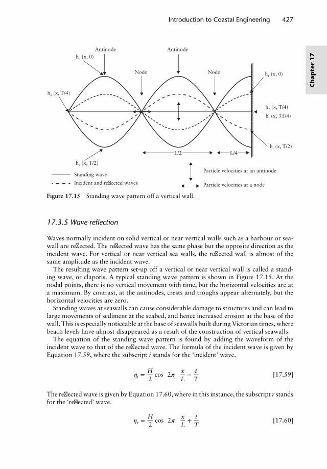
Introduction to Coastal Engineering 427
Antinode
Standing wave
hs (x, T/2)
hi (x, T/2)
hi (x, 3T/4)
hr (x, T/4)
hr (x, 0)
hs (x, 0)
hs (x, T/4)
L/2 L/4
Incident and reflected waves Particle velocities at a node
Particle velocities at an antinode
Antinode
Node Node
Figure 17.15 Standing wave pattern off a vertical wall.
17.3.5 Wave reflection
Waves normally incident on solid vertical or near vertical walls such as a harbour or sea-wall are reflected. The reflected wave has the same phase but the opposite direction as theincident wave. For vertical or near vertical sea walls, the reflected wall is almost of thesame amplitude as the incident wave.
The resulting wave pattern set-up off a vertical or near vertical wall is called a stand-ing wave, or clapotis. A typical standing wave pattern is shown in Figure 17.15. At thenodal points, there is no vertical movement with time, but the horizontal velocities are ata maximum. By contrast, at the antinodes, crests and troughs appear alternately, but thehorizontal velocities are zero.
Standing waves at seawalls can cause considerable damage to structures and can lead tolarge movements of sediment at the seabed, and hence increased erosion at the base of thewall. This is especially noticeable at the base of seawalls built during Victorian times, wherebeach levels have almost disappeared as a result of the construction of vertical seawalls.
The equation of the standing wave pattern is found by adding the waveform of theincident wave to that of the reflected wave. The formula of the incident wave is given byEquation 17.59, where the subscript i stands for the ‘incident’ wave.
𝜂i =H2cos[2𝜋( x
L− t
T
)][17.59]
The reflected wave is given by Equation 17.60, where in this instance, the subscript r standsfor the ‘reflected’ wave.
𝜂r =H2
cos[2𝜋( x
L+ t
T
)][17.60]
Ch
apte
r1
7
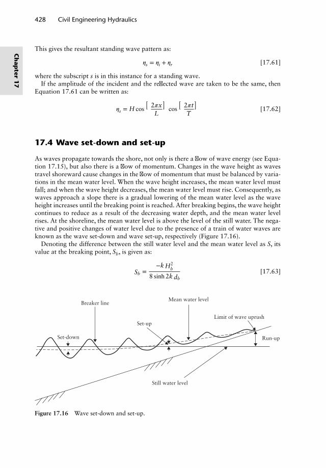
428 Civil Engineering Hydraulics
This gives the resultant standing wave pattern as:
𝜂s = 𝜂i + 𝜂r [17.61]
where the subscript s is in this instance for a standing wave.If the amplitude of the incident and the reflected wave are taken to be the same, then
Equation 17.61 can be written as:
𝜂s = H cos(
2𝜋xL
)cos(
2𝜋tT
)[17.62]
17.4 Wave set-down and set-up
As waves propagate towards the shore, not only is there a flow of wave energy (see Equa-tion 17.15), but also there is a flow of momentum. Changes in the wave height as wavestravel shoreward cause changes in the flow of momentum that must be balanced by varia-tions in the mean water level. When the wave height increases, the mean water level mustfall; and when the wave height decreases, the mean water level must rise. Consequently, aswaves approach a slope there is a gradual lowering of the mean water level as the waveheight increases until the breaking point is reached. After breaking begins, the wave heightcontinues to reduce as a result of the decreasing water depth, and the mean water levelrises. At the shoreline, the mean water level is above the level of the still water. The nega-tive and positive changes of water level due to the presence of a train of water waves areknown as the wave set-down and wave set-up, respectively (Figure 17.16).
Denoting the difference between the still water level and the mean water level as S, itsvalue at the breaking point, Sb, is given as:
Sb =−k H2
b
8 sinh2k db[17.63]
Set-down
Set-up
Run-up
Breaker lineMean water level
Limit of wave uprush
Still water level
Figure 17.16 Wave set-down and set-up.
Ch
apter
17
Introduction to Coastal Engineering 429
in which db is the depth of water at the breaking point measured to the mean water level(negative since the mean water level is below the still water level).
If we assume that shallow water conditions exist at the breaking point, then sinh2kdb ≈2kdb, giving:
Sb
db≈(
Hb
4db
)2
[17.64]
Now, the maximum value of the ratio Hb∕db is about 1.3, suggesting that the greatest set-down is about 10% of the mean water depth. However, the theory is not really valid forsuch highly non-linear conditions, and in practice, the maximum set-down is only abouthalf of this theoretical value.
The maximum set-up, Smax, occurs at the shoreline. Ignoring the small set-down at thebreaking point, then,
Smax ≈3𝛾 Hb
8[17.65]
Since the value of 𝛾 is in the range of 0.7 to 1.3, Smax is between about 25% and 50% ofthe breaking wave height.
It is clear from Equation 17.64 that a change in the breaking wave height causes a changein the set-up. Thus, when groups of waves in a natural ‘sea state’ arrive at a beach, there isa slow fluctuation in the mean water level on the beach. This is known as surf beat. Thisrise and fall in the water level causes very long, low waves to radiate seaward.
17.5 Wave impact, run-up and overtopping
17.5.1 Wave impact
Wave impact occurs when an incoming wave meets a coastal defence structure, particu-larly such as a vertical seawall, in the nearshore region. Forces caused by wave impacts arethe most intense and dangerous that a structure can suffer. Wave impact is highly depen-dent on both the wave conditions and the type of structure being considered. The typicalwave conditions of the sea state are unbroken, breaking and broken waves. When a smallamount of air is trapped between the structure and the breaking wave at the point ofimpact, the impact pressure increases considerably. Recent research studies show that airpocket dynamics play a paramount role in the evaluation of impact wave pressures (seeBullock et al., 2007; Bredmose et al., 2015).
17.5.2 Wave run-up
After a wave has broken, much of the wave energy that remains when the mass of waterreaches the shoreline is used in driving it up the face of the beach or structure. This move-ment of water up the slope is called wave run-up. The run-up, R, which is measured ver-tically above the mean surface of the sea, is the maximum height above still water level towhich the water rises, and it includes the effect of wave set-up.
Ch
apte
r1
7
430 Civil Engineering Hydraulics
The run-up on a smooth impermeable slope may be estimated with the aid of Hunt’sformula (1959) as:
Rsi
H≈ Ni
tan 𝛽√(H
L0
) (for NI ≤ 2.3 − spilling plunging waves) [17.66]
Rsi
H≈
√(𝜋
2𝛽
)+ 𝜋H
Lcot(
2𝜋dL
)(for NI > 3.2 − surging waves) [17.67]
In the range of 2.3 < NI < 3.2 (collapsing waves), Rsi may be estimated using both equa-tions, with the lower value chosen.
To allow for slope roughness and permeability, Rsi may be multiplied by a roughnessfactor r. Note, however, that Rsi cannot be less than Smax.
17.5.3 Wave overtopping
Wave overtopping occurs when a wave impacts a coastal structure, and the resultingmomentum of the wave as it breaks on the structure causes some of the water to riseabove and over the top of the structure. Based on the structure type (either permeable orimpermeable), there will be two processes taking place: wave transmission and/or passingof water (green water) over the structure. If the structure freeboard exceeds the maximumrun-up height, the overtopping occurs due to splashing (white water).
Prediction of wave overtopping is usually based on empirical formulae fitted with thehelp of experimental data. In general, overtopping is measured as mean discharge of waterper linear metre of width of the structure; for example, m3∕s∕m or l∕s∕m. The EurOtopManual (2007) highlights the latest overtopping models based on wave conditions andvariety of structure types. The manual also gives tolerable discharge values for human andstructural safety.
The principal formula employed to calculate wave overtopping (q) is of the form:
q√gH3
m0
= a exp(−bRc∕Hm0) [17.68]
where Hm0 is the significant wave height estimated from spectral analysis; Rc is the free-board of the structure; and a and b are overtopping coefficients. Rc will be replaced withRc∕𝛾, where 𝛾 is the roughness coefficient, when a structure consists of roughness elementsor roughened surface (see EurOtop Manual, 2007).
17.6 Tides, surges and mean sea level
17.6.1 Sea level
Sea levels are constantly changing under the influence of both astronomical and meteo-rological effects. The astronomical effects result in a sinusoidal variation in the sea levelsurface, which is dominated by the semi-diurnal and diurnal tide components. The mete-orological effects result in surges as a result of differential pressure changes and the wind,
Ch
apter
17
Introduction to Coastal Engineering 431
and waves as a result of the wind. A third component in the variation of the sea levelsurface, which is not easily noticeable without long-term measurements, is the tendency ofthe sea level surface to rise (or fall) over a long period of time. This is known as the ‘trend’in the sea level, and it is usually referred to as a rate in the form of ‘x mm/year’.
Sea levels relative to land can vary markedly from ‘average’ sea levels as a result of‘isostatic’ effects (often referred to as ‘glacial rebound’). During the last Ice Age, largeareas of the Northern Hemisphere such as Northern Europe and Canada were coveredwith large ice sheets. This caused the land to be pushed down. With the disappearance ofthe ice, these regions are now rising, often at a rate greater than the increase in mean sealevels. This results in the phenomenon that exists in these areas of sea levels actually fallingrelative to a fixed datum on land (e.g. at Juneau in Alaska, sea levels relative to land areestimated to be falling by 13.8 mm/year) (National Research Council, 1987).
Britain is currently rotating along an axis running from the North Welsh coastline,through Liverpool to Hull, with land levels rising to the north of this line and fallingto the south of it. The rise or fall is greater further away from this line.
17.6.2 Estimation of sea level rise
17.6.2.1 Use of tide gaugesTide gauges are fixed relative to a land datum. Therefore, tide gauges only measure ‘rel-ative’ changes in sea levels, and any calculation of trends from tide gauge data wouldneed to take local land movements into account. However, the determination of rises insea levels from tide gauge data is extremely difficult and notoriously inaccurate. Thereare several reasons for this, not least of which is the fact that long-term accurate recordsare only available from digital records, most of which have only been in place since thelate 1980s at the earliest. To determine trends in sea levels from tide gauge records wouldprobably need at least 50 years of digitally recorded data. The reason for needing sucha large data set over such a long period of time is because tides repeat themselves overa period of 18.61 years. This means that trends determined over (say) the 9-year periodbetween a peak and a trough of the 18.61-year cycle would almost certainly indicate aspurious negative trend. However, trends determined over (say) the 9-year period betweena trough and a peak of the 18.61-year cycle would almost certainly indicate a spuriouslarge positive trend.
17.6.2.2. Manually recorded sea level recordsBefore digital tide gauges were in operation, sea levels were measured manually (i.e. bywatching the sea level go up and down on a tide board and estimating the sea level fromthis observation). Long-term records of these measurements have usually been transferredinto a digital format only for the maximum recorded sea level in any particular year or,at best, the maximum recorded sea level in every month. Apart from the obvious humanerror that exists in these measurements, this technique has the added problem that thelargest sea level recorded in any one year will almost certainly correspond to a very windyday, with large onshore waves. This therefore makes the determination of the sea level tothe nearest (say) 10 cm extremely difficult, and these records are notoriously inaccurate(Hames et al., 2004) However, many of these records exist back to the mid-late nineteenthcentury, and the effect of the 18.61-year cycle of tides is therefore mostly negated.
Ch
apte
r1
7
432 Civil Engineering Hydraulics
17.6.3 Current and future trends in sea levels
The most important body who publish information on changes in sea level are the Inter-governmental Panel on Climate Change (IPCC). They have published five assessmentreports since 1988 on scientific, technical and socio-economic information related to cli-mate change, its impact and future risks, and countermeasures for adaptation and mitiga-tion. IPCC (2013) predicted the mean rate of sea level rise over the next 100 years between26 and 82 cm based on four scenarios considered. CU Sea Level Research Group (2015)presented a global mean sea level rise of 3.3 ± 0.4 mm/year for the period of 1993–2015.
Many other organisations publish reports and give guidance on sea level rises through-out the world. Apart from the IPCC, the main body responsible for analysing sea levels arethe Permanent Service for Mean Sea Level, based at the Proudman Oceanographic Labo-ratory (POL). National guidance is given by bodies such as the Environment Agency (UK).
17.7 Tsunami waves
Tsunamis are large ocean waves, or a series of waves with very large wavelengths and longperiods of up to an hour, triggered by volcanic eruptions, explosions, landslides, earth-quakes and planetary impacts. ‘Tsunami’ as a Japanese word is represented by two charac-ters which translate into English as ‘harbour wave’. Tsunamis are often incorrectly referredto as tidal waves or seismic sea waves.
In deep depths, tsunamis can be difficult to identify. There can be hundreds of kilometresbetween crests (typically 10–500 km), and the height of the wave may only be 1–2 m highat most. With several minutes passing between successive waves of a tsunami, they arehardly noticeable as they pass under ships in deep waters. When these waves approacha shoreline, however, they exhibit all the characteristics of waves covered in this chapter.Rapid draw-down of water levels can occur in harbours (i.e. set-down), often drawingpeople to the shoreline and subsequently to their deaths. Similar to water waves, when atsunami wave approaches onshore, part of the wave energy is reflected back offshore, andthe onshore propagating wave energy is dissipated through bottom friction and turbulence.Despite these losses, a tsunami waves inundates inland with a significant amount of energy,causing destruction to people, beaches and infrastructure such as coastal defences. The firstpart of the tsunami wave propagating inland can be either crest or trough-focused witha considerable amount of momentum and inertia. For example, recent studies revealedthat most coastal defences such as coastal dikes and seawalls in northern Japan collapsedby scour failure due to the great erosive power of the 2011 Tohoku tsunami waves (seeJayaratne et al., 2013, 2015; Esteban et al., 2015).
Due to large wavelengths, tsunami waves act as shallow water waves. Under such con-ditions, the wavelength is very large compared to the water depth, and the wave speeddepends only on water depth as seen in Equation 17.69:
c =√
gh [17.69]
where h is the water depth.For example, in offshore conditions, the water depth of around 5000 m generated a
tsunami speed of around 220 m/s, or about 800 km/h.The distance and height achieved by a tsunami depend on the natural contours of the
land that it approaches. Waves flowing over flat land will reach a long way inshore (large
Ch
apter
17
Introduction to Coastal Engineering 433
inundation). Waves travelling up a river valley will increase in height, and potentially floodareas to a much greater height than adjacent areas at a lower land level, which may beperhaps unaffected by the effects of the tsunami.
On land, the velocity of the tsunami wave (horizontal velocity, or u) is affected by thetopography of the land; therefore, Equation 17.69 is further modified as:
u = A√
g(R − hG) [17.70]
where hG is the height of land above mean sea level; R is the tsunami run-up height; andA is a coefficient of order 1.0 (see Murata et al., 2010).
The slowing down of the tsunami as it reaches the shore results in a shoaling wave,reaching many times its height offshore. It would not be unknown for a tsunami 1–2 mhigh in the deep depths of an ocean to reach 25–50 m by the time it reaches the shoreline(e.g. the 2004 Indian Ocean and 2011 Tohoku tsunamis). These waves will then surgeunbroken onto the land, and one of the reasons for the significant damage and loss oflife is the violent turbulent nature of the leading edge of the tsunami wave. The tsunamievent also continues for a long time after the leading edge has passed, exacerbating thedestruction caused.
The increase of the tsunami wave height as it approaches shallow water (as describedin this section) is given by:
Hs
Hd=(
hd
hs
)0.25
[17.71]
where Hs and Hd are wave heights in shallow and deep water and hs and hd are the depthsof the shallow and deep water, respectively. For example, a tsunami with a wave heightof 1 m in the open ocean where the water depth is 5000 m would have a wave heightapproaching 5 m in water of depth 10 m.
Disaster prevention or preparedness for future tsunami events was brought into focusafter the 2004 Indian Ocean tsunami. Since tsunami events are infrequent, people mayforget about the implications for them and civil engineering infrastructure. Researchersattempted to classify different levels of tsunamis (Levels 1 and 2) and gave an introduc-tion to classification of evacuation areas after the 2011 Tohoku tsunami (see Shibayama etal., 2013). The key purpose of tsunami countermeasures is to mitigate casualties, injuriesand physical damage to the infrastructure. There are two types of countermeasures beingadopted in the coastal environment, namely hard and soft engineering methods. Defencessuch as mass concrete tsunami seawalls, breakwaters, coastal dikes and high-rise evacua-tion buildings are, to name a few, hard engineering countermeasures; whilst tsunami haz-ard maps with evacuation routes and signs, and coastal forests and wetlands, are examplesof soft solutions.
Worked examples
Example 17.1
A wave in water depth of 100 m has a wave height of 3.0 m and a wave period of 12 s.Calculate wavelength, celerity and wave steepness of that wave. Check whether this waveis in shallow, transition or deep water.
Ch
apte
r1
7
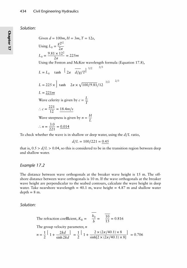
434 Civil Engineering Hydraulics
Solution:
Given d = 100m, H = 3m, T = 12s,
Using L0 =gT2
2𝜋
L0 = 9.81 × 122
2𝜋= 225m
Using the Fenton and McKee wavelength formula (Equation 17.8),
L = L0
{tanh
[(2𝜋√
d∕g∕T)3∕2
]}2∕3
L = 225 ×{tanh
[(2𝜋 ×
√100∕9.81∕12
)3∕2]}2∕3
L = 221m
Wave celerity is given by c = LT
∴ c = 22112
= 18.4m∕s
Wave steepness is given by n = HL
∴ n = 3.0221
= 0.014
To check whether the wave is in shallow or deep water, using the d∕L ratio,
d∕L = 100∕221 = 0.45
that is, 0.5 > d∕L > 0.04, so this is considered to be in the transition region between deepand shallow water.
Example 17.2
The distance between wave orthogonals at the breaker wave height is 15 m. The off-shore distance between wave orthogonals is 10 m. If the wave orthogonals at the breakerwave height are perpendicular to the seabed contours, calculate the wave height in deepwater. Take nearshore wavelength = 40.1 m, wave height = 4.87 m and shallow waterdepth = 8 m.
Solution:
The refraction coefficient, KR =
√b0
b=√
1015
= 0.816
The group velocity parameter, n
n = 12
(1 + 2kd
sinh2kd
)= 1
2
(1 +
2 × (2𝜋∕40.1) × 8sinh[2 × (2𝜋∕40.1) × 8]
)= 0.706
Ch
apter
17
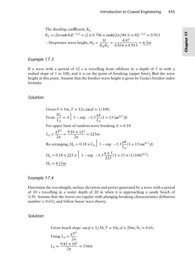
Introduction to Coastal Engineering 435
The shoaling coefficient, KS
KS = (2n tanhkd)−1∕2 = (2 × 0.706 × tanh[(2𝜋∕40.1) × 8])−1∕2 = 0.913
∴ Deepwater wave height, H0 = HKRKS
= 4.870.816 × 0.913
= 6.5m
Example 17.3
If a wave with a period of 12 s is travelling from offshore to a depth of 5 m with aseabed slope of 1 in 100, and it is on the point of breaking (upper limit), find the waveheight at this point. Assume that the breaker wave height is given by Goda’s breaker indexformula.
Solution:
Given h = 5m, T = 12s, tan 𝛽 = 1∕100,
FromHb
L0= A
{1 − exp
[−1.5𝜋h
L0(1 + 15 tan4∕3 𝛽)
]}For upper limit of random wave breaking A = 0.18
L0 =gT2
2𝜋= 9.81 × 122
2𝜋= 225m
Re-arranging, Hb = 0.18 × L0
{1 − exp
[−1.5𝜋h
L0(1 + 15 tan4∕3 𝛽)
]}
Hb = 0.18 × 225 ×{
1 − exp[−1.5𝜋 × 5
225(1 + 15 × (1∕100)4∕3)
]}Hb = 4.15m
Example 17.4
Determine the wavelength, surface elevation and power generated by a wave with a periodof 10 s travelling in a water depth of 20 m when it is approaching a sandy beach of1:30. Assume that the waves are regular with plunging breaking characteristics (Iribarrennumber = 0.65), and follow linear wave theory.
Solution:
Given beach slope tan 𝛽 = 1∕30, T = 10s, d = 20m, NI = 0.65,
Using L0 =gT2
2𝜋
L0 = 9.81 × 10²
2𝜋= 156m
Ch
apte
r1
7
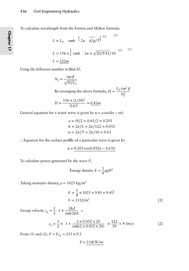
436 Civil Engineering Hydraulics
To calculate wavelength from the Fenton and McKee formula:
L = L0
{tanh
[(2𝜋√
d∕g∕T)3∕2
]}2∕3
L = 156 ×{tanh
[(2𝜋 ×
√20∕9.81∕10
)3∕2]}2∕3
L = 122m
Using the Iribarren number to find H,
NI =tan 𝛽√H∕L0
Re-arranging the above formula, H =L0 tan2 𝛽
N2I
H =156 × (1∕30)2
0.652= 0.41m
General equation for a water wave is given by 𝜂 = a cos(kx − 𝜔t)
a = H∕2 = 0.41∕2 = 0.205
k = 2𝜋∕L = 2𝜋∕122 = 0.052
𝜔 = 2𝜋∕T = 2𝜋∕10 = 0.63
∴ Equation for the surface profile of a particular wave is given by
𝜂 = 0.205 cos(0.052x − 0.63t)
To calculate power generated by the wave P,
Energy density E = 18𝜌gH2
Taking seawater density, 𝜌 = 1025 kg∕m3
E = 18× 1025 × 9.81 × 0.412
E = 211J∕m2 [1]
Group velocity cg = 12
[1 + 2kd
sinh2kd
]c
cg = 12×[1 + 2 × 0.052 × 20
sinh(2 × 0.052 × 20)
]× 122
10= 9.3m∕s [2]
From (1) and (2), P = Ecg = 211 × 9.3
P = 2.0KW∕m
Ch
apter
17
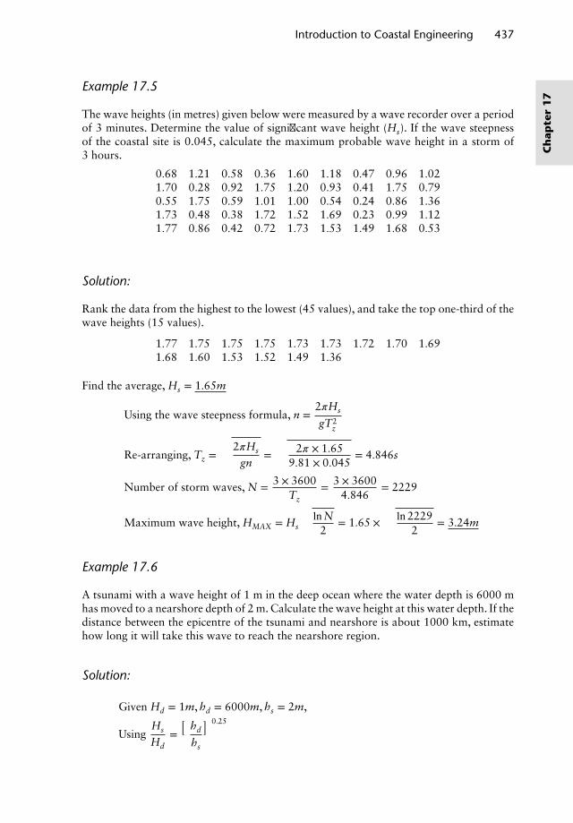
Introduction to Coastal Engineering 437
Example 17.5
The wave heights (in metres) given below were measured by a wave recorder over a periodof 3 minutes. Determine the value of significant wave height (Hs). If the wave steepnessof the coastal site is 0.045, calculate the maximum probable wave height in a storm of3 hours.
0.68 1.21 0.58 0.36 1.60 1.18 0.47 0.96 1.021.70 0.28 0.92 1.75 1.20 0.93 0.41 1.75 0.790.55 1.75 0.59 1.01 1.00 0.54 0.24 0.86 1.361.73 0.48 0.38 1.72 1.52 1.69 0.23 0.99 1.121.77 0.86 0.42 0.72 1.73 1.53 1.49 1.68 0.53
Solution:
Rank the data from the highest to the lowest (45 values), and take the top one-third of thewave heights (15 values).
1.77 1.75 1.75 1.75 1.73 1.73 1.72 1.70 1.691.68 1.60 1.53 1.52 1.49 1.36
Find the average, Hs = 1.65m
Using the wave steepness formula, n =2𝜋Hs
gT2z
Re-arranging, Tz =
√2𝜋Hs
gn=√
2𝜋 × 1.659.81 × 0.045
= 4.846s
Number of storm waves, N = 3 × 3600Tz
= 3 × 36004.846
= 2229
Maximum wave height, HMAX = Hs
√lnN
2= 1.65 ×
√ln2229
2= 3.24m
Example 17.6
A tsunami with a wave height of 1 m in the deep ocean where the water depth is 6000 mhas moved to a nearshore depth of 2 m. Calculate the wave height at this water depth. If thedistance between the epicentre of the tsunami and nearshore is about 1000 km, estimatehow long it will take this wave to reach the nearshore region.
Solution:
Given Hd = 1m, hd = 6000m, hs = 2m,
UsingHs
Hd=(
hd
hs
)0.25
Ch
apte
r1
7
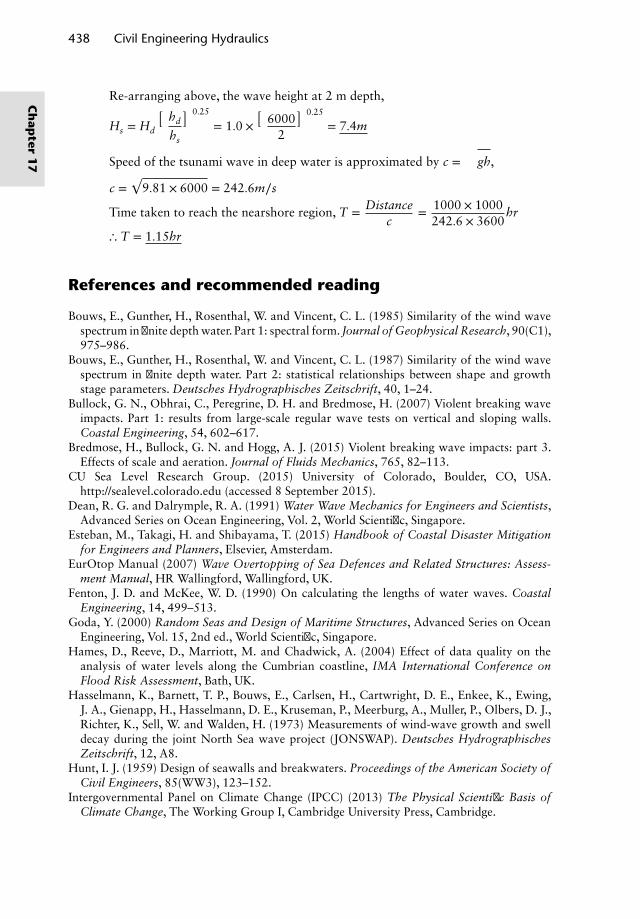
438 Civil Engineering Hydraulics
Re-arranging above, the wave height at 2 m depth,
Hs = Hd
(hd
hs
)0.25
= 1.0 ×(
60002
)0.25
= 7.4m
Speed of the tsunami wave in deep water is approximated by c =√
gh,
c =√
9.81 × 6000 = 242.6m∕s
Time taken to reach the nearshore region, T = Distancec
= 1000 × 1000242.6 × 3600
hr
∴ T = 1.15hr
References and recommended reading
Bouws, E., Gunther, H., Rosenthal, W. and Vincent, C. L. (1985) Similarity of the wind wavespectrum in finite depth water. Part 1: spectral form. Journal of Geophysical Research, 90(C1),975–986.
Bouws, E., Gunther, H., Rosenthal, W. and Vincent, C. L. (1987) Similarity of the wind wavespectrum in finite depth water. Part 2: statistical relationships between shape and growthstage parameters. Deutsches Hydrographisches Zeitschrift, 40, 1–24.
Bullock, G. N., Obhrai, C., Peregrine, D. H. and Bredmose, H. (2007) Violent breaking waveimpacts. Part 1: results from large-scale regular wave tests on vertical and sloping walls.Coastal Engineering, 54, 602–617.
Bredmose, H., Bullock, G. N. and Hogg, A. J. (2015) Violent breaking wave impacts: part 3.Effects of scale and aeration. Journal of Fluids Mechanics, 765, 82–113.
CU Sea Level Research Group. (2015) University of Colorado, Boulder, CO, USA.http://sealevel.colorado.edu (accessed 8 September 2015).
Dean, R. G. and Dalrymple, R. A. (1991) Water Wave Mechanics for Engineers and Scientists,Advanced Series on Ocean Engineering, Vol. 2, World Scientific, Singapore.
Esteban, M., Takagi, H. and Shibayama, T. (2015) Handbook of Coastal Disaster Mitigationfor Engineers and Planners, Elsevier, Amsterdam.
EurOtop Manual (2007) Wave Overtopping of Sea Defences and Related Structures: Assess-ment Manual, HR Wallingford, Wallingford, UK.
Fenton, J. D. and McKee, W. D. (1990) On calculating the lengths of water waves. CoastalEngineering, 14, 499–513.
Goda, Y. (2000) Random Seas and Design of Maritime Structures, Advanced Series on OceanEngineering, Vol. 15, 2nd ed., World Scientific, Singapore.
Hames, D., Reeve, D., Marriott, M. and Chadwick, A. (2004) Effect of data quality on theanalysis of water levels along the Cumbrian coastline, IMA International Conference onFlood Risk Assessment, Bath, UK.
Hasselmann, K., Barnett, T. P., Bouws, E., Carlsen, H., Cartwright, D. E., Enkee, K., Ewing,J. A., Gienapp, H., Hasselmann, D. E., Kruseman, P., Meerburg, A., Muller, P., Olbers, D. J.,Richter, K., Sell, W. and Walden, H. (1973) Measurements of wind-wave growth and swelldecay during the joint North Sea wave project (JONSWAP). Deutsches HydrographischesZeitschrift, 12, A8.
Hunt, I. J. (1959) Design of seawalls and breakwaters. Proceedings of the American Society ofCivil Engineers, 85(WW3), 123–152.
Intergovernmental Panel on Climate Change (IPCC) (2013) The Physical Scientific Basis ofClimate Change, The Working Group I, Cambridge University Press, Cambridge.
Ch
apter
17
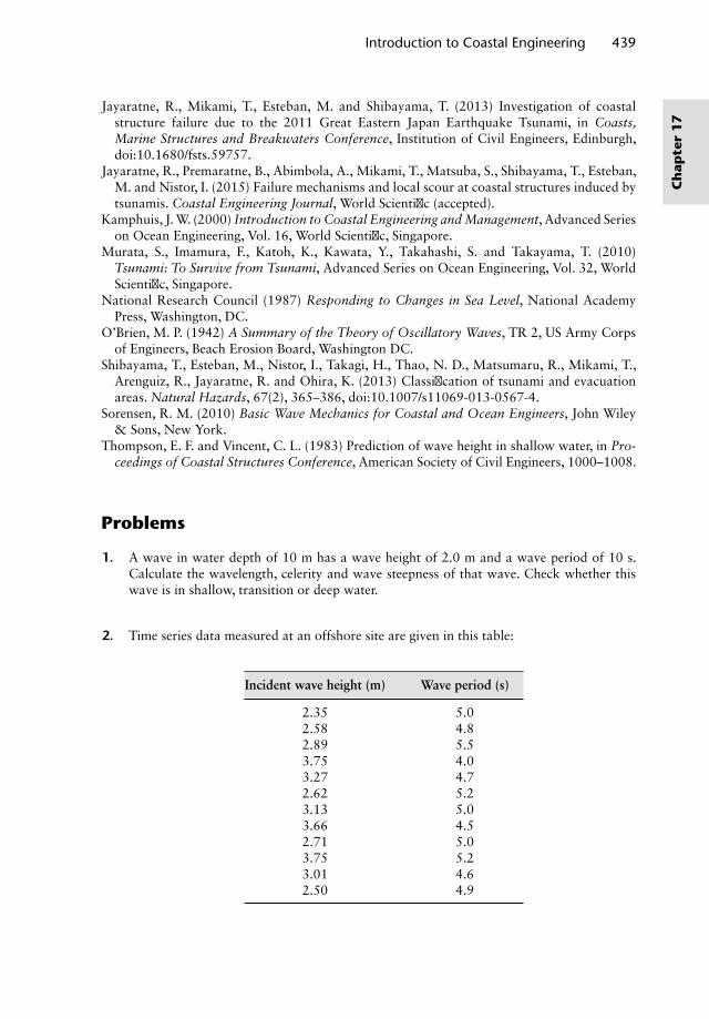
Introduction to Coastal Engineering 439
Jayaratne, R., Mikami, T., Esteban, M. and Shibayama, T. (2013) Investigation of coastalstructure failure due to the 2011 Great Eastern Japan Earthquake Tsunami, in Coasts,Marine Structures and Breakwaters Conference, Institution of Civil Engineers, Edinburgh,doi:10.1680/fsts.59757.
Jayaratne, R., Premaratne, B., Abimbola, A., Mikami, T., Matsuba, S., Shibayama, T., Esteban,M. and Nistor, I. (2015) Failure mechanisms and local scour at coastal structures induced bytsunamis. Coastal Engineering Journal, World Scientific (accepted).
Kamphuis, J. W. (2000) Introduction to Coastal Engineering and Management, Advanced Serieson Ocean Engineering, Vol. 16, World Scientific, Singapore.
Murata, S., Imamura, F., Katoh, K., Kawata, Y., Takahashi, S. and Takayama, T. (2010)Tsunami: To Survive from Tsunami, Advanced Series on Ocean Engineering, Vol. 32, WorldScientific, Singapore.
National Research Council (1987) Responding to Changes in Sea Level, National AcademyPress, Washington, DC.
O’Brien, M. P. (1942) A Summary of the Theory of Oscillatory Waves, TR 2, US Army Corpsof Engineers, Beach Erosion Board, Washington DC.
Shibayama, T., Esteban, M., Nistor, I., Takagi, H., Thao, N. D., Matsumaru, R., Mikami, T.,Arenguiz, R., Jayaratne, R. and Ohira, K. (2013) Classification of tsunami and evacuationareas. Natural Hazards, 67(2), 365–386, doi:10.1007/s11069-013-0567-4.
Sorensen, R. M. (2010) Basic Wave Mechanics for Coastal and Ocean Engineers, John Wiley& Sons, New York.
Thompson, E. F. and Vincent, C. L. (1983) Prediction of wave height in shallow water, in Pro-ceedings of Coastal Structures Conference, American Society of Civil Engineers, 1000–1008.
Problems
1. A wave in water depth of 10 m has a wave height of 2.0 m and a wave period of 10 s.Calculate the wavelength, celerity and wave steepness of that wave. Check whether thiswave is in shallow, transition or deep water.
2. Time series data measured at an offshore site are given in this table:
Incident wave height (m) Wave period (s)
2.35 5.02.58 4.82.89 5.53.75 4.03.27 4.72.62 5.23.13 5.03.66 4.52.71 5.03.75 5.23.01 4.62.50 4.9
Ch
apte
r1
7
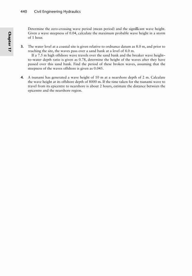
440 Civil Engineering Hydraulics
Determine the zero-crossing wave period (mean period) and the significant wave height.Given a wave steepness of 0.04, calculate the maximum probable wave height in a stormof 1 hour.
3. The water level at a coastal site is given relative to ordnance datum as 8.0 m, and prior toreaching the site, the waves pass over a sand bank at a level of 4.0 m.
If a 7.5 m high offshore wave travels over the sand bank and the breaker wave height–to–water depth ratio is given as 0.78, determine the height of the waves after they havepassed over this sand bank. Find the period of these broken waves, assuming that thesteepness of the waves offshore is given as 0.045.
4. A tsunami has generated a wave height of 10 m at a nearshore depth of 2 m. Calculatethe wave height at its offshore depth of 8000 m. If the time taken for the tsunami wave totravel from its epicentre to nearshore is about 2 hours, estimate the distance between theepicentre and the nearshore region.
Ch
apter
17
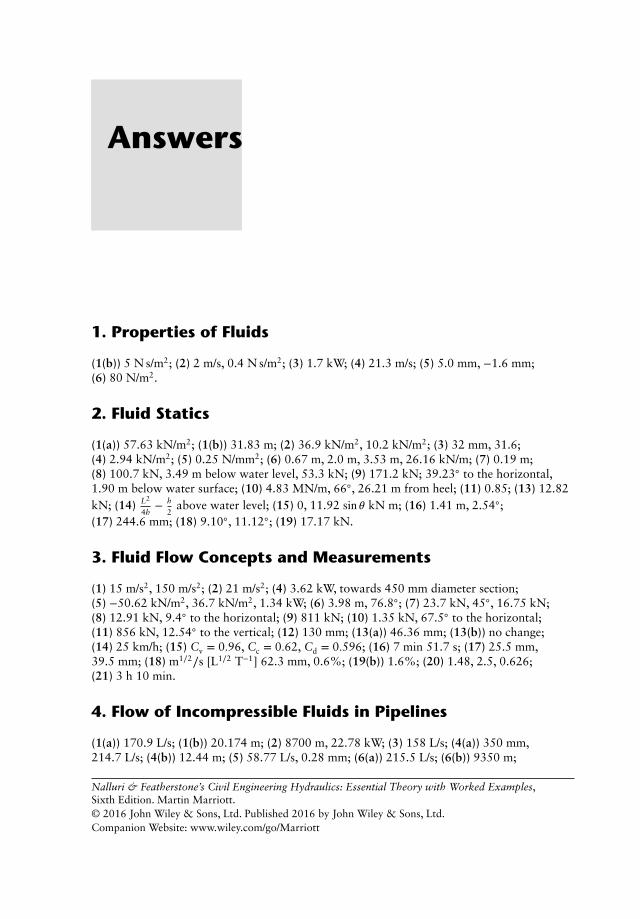
Answers
1. Properties of Fluids
(1(b)) 5 N s/m2; (2) 2 m/s, 0.4 N s/m2; (3) 1.7 kW; (4) 21.3 m/s; (5) 5.0 mm, −1.6 mm;(6) 80 N/m2.
2. Fluid Statics
(1(a)) 57.63 kN/m2; (1(b)) 31.83 m; (2) 36.9 kN/m2, 10.2 kN/m2; (3) 32 mm, 31.6;(4) 2.94 kN/m2; (5) 0.25 N/mm2; (6) 0.67 m, 2.0 m, 3.53 m, 26.16 kN/m; (7) 0.19 m;(8) 100.7 kN, 3.49 m below water level, 53.3 kN; (9) 171.2 kN; 39.23◦ to the horizontal,1.90 m below water surface; (10) 4.83 MN/m, 66◦, 26.21 m from heel; (11) 0.85; (13) 12.82kN; (14) L2
4h− h
2above water level; (15) 0, 11.92 sin 𝜃 kN m; (16) 1.41 m, 2.54◦;
(17) 244.6 mm; (18) 9.10◦, 11.12◦; (19) 17.17 kN.
3. Fluid Flow Concepts and Measurements
(1) 15 m/s2, 150 m/s2; (2) 21 m/s2; (4) 3.62 kW, towards 450 mm diameter section;(5) −50.62 kN/m2, 36.7 kN/m2, 1.34 kW; (6) 3.98 m, 76.8◦; (7) 23.7 kN, 45◦, 16.75 kN;(8) 12.91 kN, 9.4◦ to the horizontal; (9) 811 kN; (10) 1.35 kN, 67.5◦ to the horizontal;(11) 856 kN, 12.54◦ to the vertical; (12) 130 mm; (13(a)) 46.36 mm; (13(b)) no change;(14) 25 km/h; (15) Cv = 0.96, Cc = 0.62, Cd = 0.596; (16) 7 min 51.7 s; (17) 25.5 mm,39.5 mm; (18) m1∕2∕s [L1∕2 T−1] 62.3 mm, 0.6%; (19(b)) 1.6%; (20) 1.48, 2.5, 0.626;(21) 3 h 10 min.
4. Flow of Incompressible Fluids in Pipelines
(1(a)) 170.9 L/s; (1(b)) 20.174 m; (2) 8700 m, 22.78 kW; (3) 158 L/s; (4(a)) 350 mm,214.7 L/s; (4(b)) 12.44 m; (5) 58.77 L/s, 0.28 mm; (6(a)) 215.5 L/s; (6(b)) 9350 m;
Nalluri & Featherstone’s Civil Engineering Hydraulics: Essential Theory with Worked Examples,Sixth Edition. Martin Marriott.© 2016 John Wiley & Sons, Ltd. Published 2016 by John Wiley & Sons, Ltd.Companion Website: www.wiley.com/go/Marriott
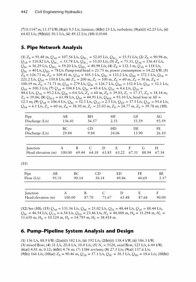
442 Civil Engineering Hydraulics
(7) 0.1147 m,13.37 kW; (8(a)) 9.5 L/s, laminar; (8(b)) 25 L/s, turbulent; (9(a)(i)) 62.25 L/s, (ii)64.82 L/s; (9(b)(i)) 50.1 L/s, (ii) 49.12 L/s; (10) 0.0144.
5. Pipe Network Analysis
(1) ZB = 91.48 m, QAB = 107.56 L/s, QBC1= 52.05 L/s, QBC2
= 55.51 L/s; (2) ZB = 90.98 m,QAB = 110.82 L/s, QBC1
= 55.78 L/s, QBC2= 55.03 L/s; (3) ZB = 75.31, QAB = 156.43 L/s,
QBC = 56.29 L/s, QBD1= 59.20 L/s, QBD2
= 40.98 L/s; (4) ZB = 132.3 m, QAB = 118 L/s,QBC = 40 L/s,QBD = 78 L/s.Pump total head = 21.75 m, power consumption = 14.22 kW; (5)ZB = 126.73 m, ZD = 109.41 m, QAB = 505.3 L/s, QBC = 133.2 L/s, QBD = 372.1 L/s, QDE =221.2 L/s, QDF = 150.8 L/s; (6) ZA = 200 m, ZC = 100 m, ZE = 60 m, ZF = 50 m, ZB =100.19 m, ZD = 71.71 m, QAB = 279 L/s, QBC = 126.7 L/s, QBD = 152.4 L/s, QDE = 52.1 L/s,QDF = 100.3 L/s; (7) QAB = 104.8 L/s, QBC = 45.4 L/s, QDC = 4.6 L/s, QED =44.6 L/s, QAE = 95.2 L/s, QEB = 0.6 L/s, ZA = 60 m, ZB = 39.03, ZC = 17.37, ZD = 18.14 m,ZE = 39.06; (8) QBCE = 61.98 L/s, QBE = 44.91 L/s, QBDE = 93.10 L/s, head loss in AF =12.5 m; (9) QAB = 106.4 L/s, QBC = 52.5 L/s, QCD = 2.5 L/s, QED = 37.5 L/s, QAE = 93.6 L/s,QEB = 6.1 L/s, ZA = 60 m, ZB = 38.50 m, ZC = 25.03 m, ZD = 24.77 m, ZE = 39.78 m; (10).
Pipe AB BH HF GF AGDischarge (L/s) 136.41 56.57 2.51 53.59 93.59
Pipe BC CD HD DE FEDischarge (L/s) 29.84 9.84 24.06 13.90 26.10
Junction A B C D E F G HHead elevation (m) 100.00 69.44 64.18 63.85 63.22 67.31 88.94 67.34
(11)
Pipe AB BC CD ED FE BEFlow (L/s) 95.31 90.14 30.14 49.86 44.69 5.17
Junction A B C D E FHead elevation (m) 100.00 87.70 71.67 65.48 87.66 90.00
(12) See (10); (13) QAB = 131.56 L/s, QBE = 25.02 L/s, QFE = 48.44 L/s, QAF = 88.44 L/s,QBC = 46.54 L/s, QCD = 6.54 L/s, QED = 23.46 L/s; HA = 40.000 m, HB = 31.294 m, HC =11.650 m, HD = 10.124 m, HE = 14.795 m, HF = 38.418 m.
6. Pump–Pipeline System Analysis and Design
(1) 136 L/s, 88.9 kW; (2(a)(i)) 182 L/s, (ii) 192 L/s; (2(b)(i)) 138.4 kW, (ii) 186.3 kW;(3) mixed flow; (4) 31 L/s, 20.8 L/s, 10.0 L/s; (5) Ns = 5120, axial flow, 125 L/s, 6.44 kW;(6(a)) 4.81 m, 0.12; (6(b)) 4.76 m; (7) 1386 rev/min; (8) 27.5 L/s; (9(a)) 137.6 L/s;(9(b)) 166 L/s; (10(a)) ZB = 90.46 m, QAB = 57.1 L/s, QBC = 38.5 L/s, QBD = 18.6 L/s; (10(b))
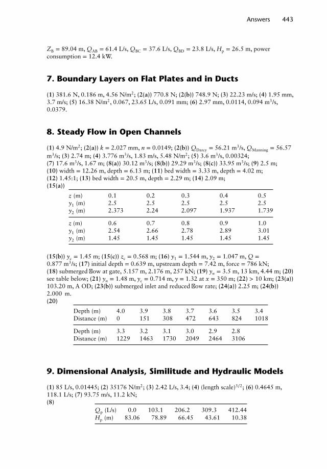
Answers 443
ZB = 89.04 m, QAB = 61.4 L/s, QBC = 37.6 L/s, QBD = 23.8 L/s, Hp = 26.5 m, powerconsumption = 12.4 kW.
7. Boundary Layers on Flat Plates and in Ducts
(1) 381.6 N, 0.186 m, 4.56 N/m2; (2(a)) 770.8 N; (2(b)) 748.9 N; (3) 22.23 m/s; (4) 1.95 mm,3.7 m/s; (5) 16.38 N/m2, 0.067, 23.65 L/s, 0.091 mm; (6) 2.97 mm, 0.0114, 0.094 m3/s,0.0379.
8. Steady Flow in Open Channels
(1) 4.9 N/m2; (2(a)) k = 2.027 mm, n = 0.0149; (2(b)) QDarcy = 56.21 m3/s, QManning = 56.57m3/s; (3) 2.74 m; (4) 3.776 m3/s, 1.83 m/s, 5.48 N/m2; (5) 3.6 m3/s, 0.00324;(7) 17.6 m3/s, 1.67 m; (8(a)) 30.12 m3/s; (8(b)) 29.29 m3/s; (8(c)) 33.95 m3/s; (9) 2.5 m;(10) width = 12.26 m, depth = 6.13 m; (11) bed width = 3.33 m, depth = 4.02 m;(12) 1.45:1; (13) bed width = 20.5 m, depth = 2.29 m; (14) 2.09 m;(15(a))
z (m) 0.1 0.2 0.3 0.4 0.5y1 (m) 2.5 2.5 2.5 2.5 2.5y2 (m) 2.373 2.24 2.097 1.937 1.739
z (m) 0.6 0.7 0.8 0.9 1.0y1 (m) 2.54 2.66 2.78 2.89 3.01y2 (m) 1.45 1.45 1.45 1.45 1.45
(15(b)) yc = 1.45 m; (15(c)) zc = 0.568 m; (16) y1 = 1.544 m, y2 = 1.047 m, Q =0.877 m3/s; (17) initial depth = 0.639 m, upstream depth = 7.42 m, force = 786 kN;(18) submerged flow at gate, 5.157 m, 2.176 m, 257 kN; (19) yn = 3.5 m, 13 km, 4.44 m; (20)see table below; (21) yn = 1.48 m, yc = 0.714 m, y = 1.32 at x = 350 m; (22) > 10 km; (23(a))103.20 m, A OD; (23(b)) submerged inlet and reduced flow rate; (24(a)) 2.25 m; (24(b))2.000 m.(20)
Depth (m) 4.0 3.9 3.8 3.7 3.6 3.5 3.4Distance (m) 0 151 308 472 643 824 1018
Depth (m) 3.3 3.2 3.1 3.0 2.9 2.8Distance (m) 1229 1463 1730 2049 2464 3106
9. Dimensional Analysis, Similitude and Hydraulic Models
(1) 85 L/s, 0.01445; (2) 35176 N/m2; (3) 2.42 L/s, 3.4; (4) (length scale)3∕2; (6) 0.4645 m,118.1 L/s; (7) 93.75 m/s, 11.2 kN;(8)
Qp (L/s) 0.0 103.1 206.2 309.3 412.44Hp (m) 83.06 78.89 66.45 43.61 10.38
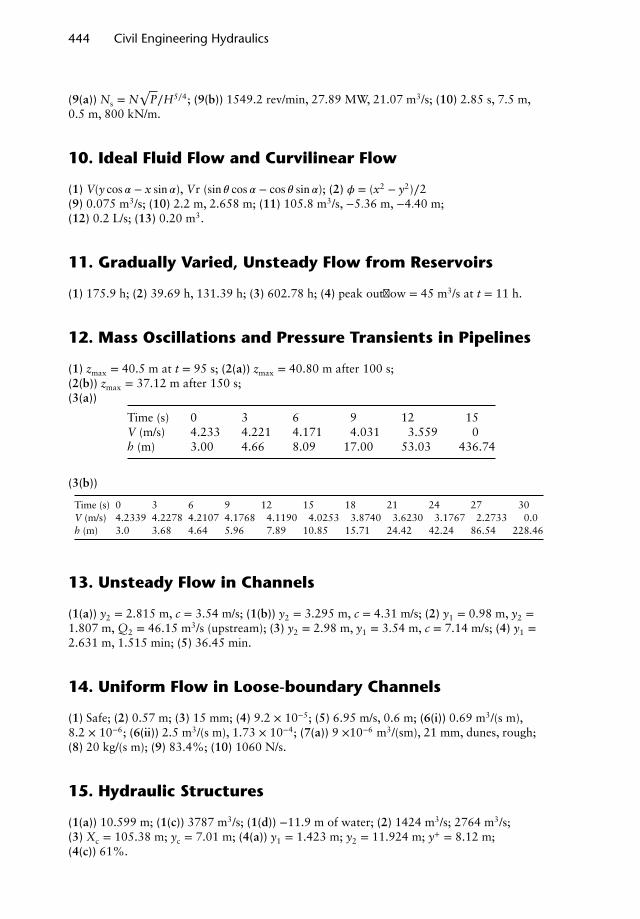
444 Civil Engineering Hydraulics
(9(a)) Ns = N√
P∕H5∕4; (9(b)) 1549.2 rev/min, 27.89 MW, 21.07 m3/s; (10) 2.85 s, 7.5 m,0.5 m, 800 kN/m.
10. Ideal Fluid Flow and Curvilinear Flow
(1) V(y cos 𝛼 − x sin 𝛼), Vr (sin 𝜃 cos 𝛼 − cos 𝜃 sin 𝛼); (2) 𝜙 = (x2 − y2)∕2(9) 0.075 m3/s; (10) 2.2 m, 2.658 m; (11) 105.8 m3/s, −5.36 m, −4.40 m;(12) 0.2 L/s; (13) 0.20 m3.
11. Gradually Varied, Unsteady Flow from Reservoirs
(1) 175.9 h; (2) 39.69 h, 131.39 h; (3) 602.78 h; (4) peak outflow = 45 m3/s at t = 11 h.
12. Mass Oscillations and Pressure Transients in Pipelines
(1) zmax = 40.5 m at t = 95 s; (2(a)) zmax = 40.80 m after 100 s;(2(b)) zmax = 37.12 m after 150 s;(3(a))
Time (s) 0 3 6 9 12 15V (m/s) 4.233 4.221 4.171 4.031 3.559 0h (m) 3.00 4.66 8.09 17.00 53.03 436.74
(3(b))
Time (s) 0 3 6 9 12 15 18 21 24 27 30V (m/s) 4.2339 4.2278 4.2107 4.1768 4.1190 4.0253 3.8740 3.6230 3.1767 2.2733 0.0h (m) 3.0 3.68 4.64 5.96 7.89 10.85 15.71 24.42 42.24 86.54 228.46
13. Unsteady Flow in Channels
(1(a)) y2 = 2.815 m, c = 3.54 m/s; (1(b)) y2 = 3.295 m, c = 4.31 m/s; (2) y1 = 0.98 m, y2 =1.807 m, Q2 = 46.15 m3/s (upstream); (3) y2 = 2.98 m, y1 = 3.54 m, c = 7.14 m/s; (4) y1 =2.631 m, 1.515 min; (5) 36.45 min.
14. Uniform Flow in Loose-boundary Channels
(1) Safe; (2) 0.57 m; (3) 15 mm; (4) 9.2 × 10⁻⁵; (5) 6.95 m/s, 0.6 m; (6(i)) 0.69 m3/(s m),8.2 × 10−6; (6(ii)) 2.5 m3/(s m), 1.73 × 10⁻⁴; (7(a)) 9 ×10⁻⁶ m3/(sm), 21 mm, dunes, rough;(8) 20 kg/(s m); (9) 83.4%; (10) 1060 N/s.
15. Hydraulic Structures
(1(a)) 10.599 m; (1(c)) 3787 m3/s; (1(d)) −11.9 m of water; (2) 1424 m3/s; 2764 m3/s;(3) Xc = 105.38 m; yc = 7.01 m; (4(a)) y1 = 1.423 m; y2 = 11.924 m; y+ = 8.12 m;(4(c)) 61%.
Answers 445
16. Environmental Hydraulics and Engineering Hydrology
(1) 41 m3∕s; (2) 0.144; (3) 9 m3∕s just after t = 4 h (4(a)) 1120 m3∕s; (4(b)) 2360 m3∕s;(5) Scheme B, 2.2.
17. Introduction to Coastal Engineering
(1) 94 m, 9.4 m/s, 0.021, transition; (2) 4.87 s, 3.61 m, 6.34 m; (3) 3.12 m, 10.3 s;(4) 1.26 m, 2017 km.


Index
absolute pressure, 10acceleration
centrifugal, 23convective, 50horizontal, 22local, 50normal, 50radial, 23tangential, 50uniform linear, 22vertical, 22
Ackers–White, 346Airy, 409, 411alluvial, 337angular velocity, 23antidune, 335Archimedes, principle of, 17atmospheric pressure, 9
backwater curves in channels, 187, 234Barr, 91, 93beach slope, 425–426, 435bed forms, 335bed hydraulic radius, 337bed load, 340bed shear, 335benefits, 397Bernoulli’s equation, 53Blasius, 90, 171
boundary layersboundary shear stress, 89, 172displacement thickness, 173drag, 172–173effect of plate roughness, 171flat plates, 172–173Karman–Prandtl equations, 176laminar boundary layers, 171laminar sub-layer, 176mixing length, 174Nikuradse, 175–176Prandtl mixing theory, 174shear velocity, 174thickness, 171turbulent boundary layers, 172turbulent pipe flow, 174
Boussinesq, coefficient of, 57, 197bulk modulus, 2, 248
effect on wave speed, 311buoyancy, centre of, 18buoyant thrust, 17
canal delivery, 201capillarity, 3cavitation, 55, 59, 153
number, 154celerity, 309, 323, 411, 413–414centrifugal pumps, 149channels, see open channel flow
Nalluri & Featherstone’s Civil Engineering Hydraulics: Essential Theory with Worked Examples,Sixth Edition. Martin Marriott.© 2016 John Wiley & Sons, Ltd. Published 2016 by John Wiley & Sons, Ltd.Companion Website: www.wiley.com/go/Marriott

448 Index
characteristic curves, pumps, 151–153Chezy equation, 189climate change, 396, 432coastal engineering, 409Colebrook–White, 91, 176, 188, 247, 251compressibility, 2concentration, 217, 343continuity, equation of, 50, 120, 306, 311
two-dimensional flow, 265contraction, coefficient of, 57, 61Coriolis coefficient, 55, 187corresponding speed, 255cost–benefit analysis, 397critical depth, 196critical shear, 335critical velocity, 196culvert, 202, 237–239curved surface, hydrostatic thrust, 15curvilinear flow, 273
channel bend, 284duct bend, 278–281rotating cylinder, 281siphon spillway, 282–283
Darcy–Weisbach equation, 90, 188density, mass, 2
relative density, 2, 336specific volume, 4specific weight, 2
diffraction, 423–434dimensional analysis, 247
Buckingham 𝜋 theorem, 249corresponding speed, 255dimensional forms, 248Froude number, 249–262model studies, 249, 257–259, 262non-dimensional groups, 248pipelines, 250prototype, 247rectangular weir, 254Reynolds number, 248–249, 254, 256–257rotodynamic pumps, 251–252, 260–262similitude, 249V-notch, 253, 256Weber number, 249, 254, 256–257
discharge, 50coefficient of, 59, 61, 371, 373under varying head, 63, 289
discounted cash flow, 397displacement thickness, 173drag coefficient, 340
drag, flow over flat plate, 172dunes, 335dynamic similarity, 249
eddy viscosity, 52, 343Einstein’s equation, 339, 342, 345energy
equation for ideal fluid flow, 52equation for real, incompressible flow, 54gradient, 89, 188kinetic, 54potential, 54pressure, 54total, 54
energy dissipators, 376energy equation, 52, 54, 89, 187, 195energy losses
flowing fluid, 89, 198pipes, 54, 89sudden transitions, 57, 95
Engelund, 345environment, 393equilibrium
neutral, 18relative, 22stable, 18unstable, 18
equipotential lines, 267estuary models, 259Euler’s equation of motion, 53
fall velocity, 339Fenton and McKee, 412fetch, 247, 418, 420floating bodies
equilibrium of, 18liquid ballast, 20periodic time of oscillation, 20stability of, 17
flood alleviation, 396flood routing, 291, 299–301, 396flow
channels, 187, 323curvilinear, 273dynamics of, 52Eulerian description of, 47gradually varied, steady, 198–200gradually varied, unsteady, 289, 323ideal, 52, 265incompressible fluids in pipelines, 89–118irrotational, 49

Index 449
kinematics of, 47Lagrangian description of, 47laminar, 51, 90, 92measurement of, see flow measurementnon-uniform, 48one dimensional, 49pipe networks, 119–148rapidly varied, steady, 195rapidly varied, unsteady, see pressure
transients, waterhammer, surgereal, 54rotational, 49subcritical, 196supercritical, 196steady, 48, 195, 198–199three dimensional, 49turbulent, 51, 91–92two dimensional, 49uniform, 48unsteady, 48, 287, 323
flow measurement, 58–68, 218–221, 227,376
flow nets, 268, 270, 275, 279flow regimes, 335fluid
definition of, 1flow concepts and measurements, see flow,
flow measurementideal, definition, 52Newtonian, 1–2
fluid statics, 7fluids in relative equilibrium, 22
effect of acceleration, 22–23fluids, real and ideal, 52, 54, 265force exerted by a jet on a flat plate, 77–78force on pipe bend, 76forced vortex, 274, 281form drag, 337free vortex, 274friction factor
dependence on Reynolds number, 90–92laminar flow, 90, 92rough pipes, 91–94smooth pipes, 90–92turbulent flow, 90–94
friction losses in pipes, 89–90Froude number, 196–197, 249–262, 323,
335
Garde, 345Garde–Ranga Raju’s formula, 337
gas, definition of, 1generalised logistic distribution, 395,
398–403geometric similarity, 247Goda’s index and formulae, 426gradually varied flow, see flowGraf, 345grain resistance, 337Gringorten, 394, 398, 402–403group wave celerity, 414Gumbel distribution, 394, 398, 402
Hagen–Poiseuille equation, 90, 247Hardy-Cross, 120head
potential or elevation, 54pressure, 9, 54varying, 63velocity or kinetic, 54
HR Wallingford design chart, 93hydraulic grade line, 89, 150hydraulic jump, 196–198, 376–378hydraulic radius, 90, 336hydraulic structures, 371hydrograph, 299–301, 396hydrological cycle, 393hydrology, 393hydrostatic thrust (force)
curved surface, 15plane surface, 11
ideal fluid flow, 52, 265boundary conditions, 272circulation, 267combination of basic flow patterns, 269curvilinear flow, 273, 281equipotential lines, 267flow nets, 268, 270, 275, 279forced vortex, 274, 281free vortex, 274graphical methods, 275Laplace equation, 270line sink, 269line source, 268numerical methods, 270pathline, 47, 265radial velocity component, 266siphon spillway, 282stream function, 265, 267streamlines, 47, 265streamtube, 49, 265

450 Index
ideal fluid flow (Continued)tangential velocity component, 266uniform flow pattern, 268
impeller, 149, 260–262incipient motion, 335Iribarren number, 425irrotational flow, 49, 265
JONSWAP wave spectrum, 418
Kalinske, 341, 344Karman–Prandtl equations, 91, 176Karman’s constant, 343kinetic energy correction factor, 55
Lacey, 337laminar boundary layer, 171laminar flow, 51laminar sub-layer, 176Lane and Kalinske, 344Laplace’s equation, 270Laursen, 345liquid, definition of, 1logarithmic velocity distribution, 174loose-boundary, 335losses
in pipe fittings, 94sudden contraction, 57sudden enlargement, 57
Manning formula, 189, 193, 336, 396manometer
differential, 10inclined, 10U-tube, 10
mass oscillations in pipelinesfinite difference methods, 308sudden discharge stoppage, 306–307surge chamber operation, 305
meandering, 396metacentre, 18metacentric height, 18, 20Meyer–Peter and Muller’s equation, 341model studies, see dimensional analysismodel testing, see similitudemomentum
correction factor, 56equation, 56, 77, 196
Moody diagram, 92mouthpieces, 61
hydraulic coefficients of, 61movability parameter, 339, 343–344
negative surge, 327net positive suction head, 154Newtonian fluid, 1–2Newton’s law of motion, 56, 248Newton’s law of viscosity, 2Nikuradse, 91, 175–176notches, 64
Bazin formula, 65end contractions, 65Francis formula, 65rectangular, 64Rehbock formula, 65trapezoidal, 66V or triangular, 65
ogee spillway, 67, 371–372open channel flow (steady)
best hydraulic section, 191channel design, 191Chezy equation, 189, 208Colebrook–White equation, 188composite roughness, 189compound section, 190, 210conveyance of river and flood plain,
396critical depth flume, 228critical tractive force, 192–193, 337Darcy–Weisbach equation, 188economic section, 191energy components, 195energy principles, 195flow measurement, 64–68, 218–221gradually varied flow, 198–200hydraulic jump, 196–198, 376–378Manning formula, 189, 193, 336,
396mobile boundary, 192momentum equation, 196part-full circular pipes, 194, 216rapidly varied flow, 195rigid boundary, 191sewers, 194spatially varied flow, 203specific energy, 195storm sewer, 194, 217uniform flow, 187uniform flow resistance, 188velocity distribution, 207venturi flume, 221, 228–229wastewater sewer, 194, 215water surface profile, 234–235wetted perimeter, 191, 339
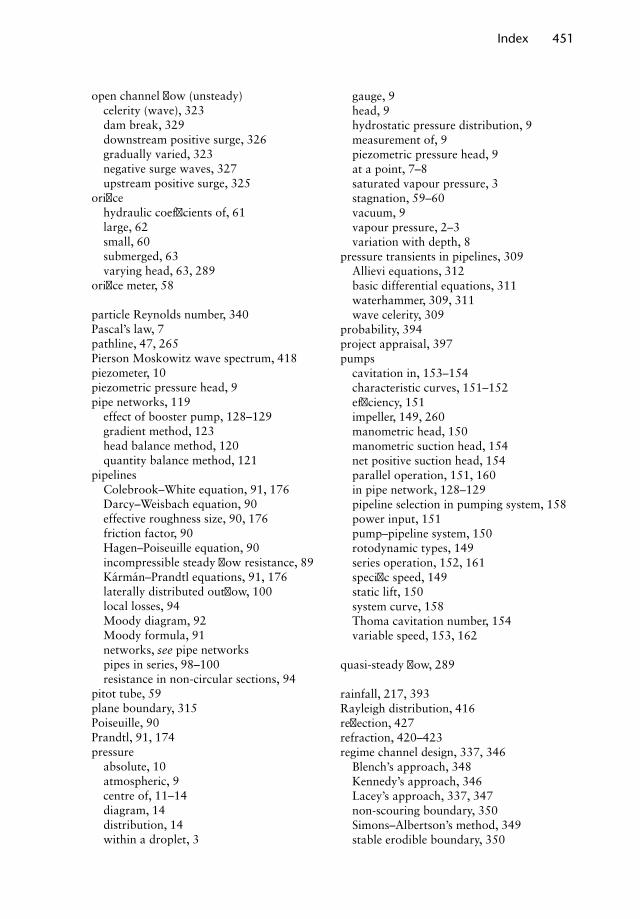
Index 451
open channel flow (unsteady)celerity (wave), 323dam break, 329downstream positive surge, 326gradually varied, 323negative surge waves, 327upstream positive surge, 325
orificehydraulic coefficients of, 61large, 62small, 60submerged, 63varying head, 63, 289
orifice meter, 58
particle Reynolds number, 340Pascal’s law, 7pathline, 47, 265Pierson Moskowitz wave spectrum, 418piezometer, 10piezometric pressure head, 9pipe networks, 119
effect of booster pump, 128–129gradient method, 123head balance method, 120quantity balance method, 121
pipelinesColebrook–White equation, 91, 176Darcy–Weisbach equation, 90effective roughness size, 90, 176friction factor, 90Hagen–Poiseuille equation, 90incompressible steady flow resistance, 89Karman–Prandtl equations, 91, 176laterally distributed outflow, 100local losses, 94Moody diagram, 92Moody formula, 91networks, see pipe networkspipes in series, 98–100resistance in non-circular sections, 94
pitot tube, 59plane boundary, 315Poiseuille, 90Prandtl, 91, 174pressure
absolute, 10atmospheric, 9centre of, 11–14diagram, 14distribution, 14within a droplet, 3
gauge, 9head, 9hydrostatic pressure distribution, 9measurement of, 9piezometric pressure head, 9at a point, 7–8saturated vapour pressure, 3stagnation, 59–60vacuum, 9vapour pressure, 2–3variation with depth, 8
pressure transients in pipelines, 309Allievi equations, 312basic differential equations, 311waterhammer, 309, 311wave celerity, 309
probability, 394project appraisal, 397pumps
cavitation in, 153–154characteristic curves, 151–152efficiency, 151impeller, 149, 260manometric head, 150manometric suction head, 154net positive suction head, 154parallel operation, 151, 160in pipe network, 128–129pipeline selection in pumping system, 158power input, 151pump–pipeline system, 150rotodynamic types, 149series operation, 152, 161specific speed, 149static lift, 150system curve, 158Thoma cavitation number, 154variable speed, 153, 162
quasi-steady flow, 289
rainfall, 217, 393Rayleigh distribution, 416reflection, 427refraction, 420–423regime channel design, 337, 346
Blench’s approach, 348Kennedy’s approach, 346Lacey’s approach, 337, 347non-scouring boundary, 350Simons–Albertson’s method, 349stable erodible boundary, 350

452 Index
Rehbock formula, 65relative density, 2, 336relative roughness, 90reservoir routing, 291, 299–301return period, 194, 394Reynolds number, 52, 90, 249–262Riemann, 313rigid-bed channels
friction factors, 351–352limit deposition, 350–352sediment transport, 350
ripples, 335river models, 257–258rotational flow, 49, 265, 273roughness, 90Rouse’s distribution, 343Runge–Kutta method, 240runoff, 194, 217, 393
saltation, 340, 344Schoklitsch’s equation, 341sea level, 430–432sediment, 194, 335sediment transport, 335, 350, 396self-cleansing velocity, 194, 216, 351separation, 55sewers, 187, 194, 350shear Reynolds number, 335shear stress, 1, 7, 89, 171, 192–193,
335shear velocity, 174, 336Shields criterion and diagram, 336Shields transport equation, 341side weir, 204similitude, similarity, 247, 249
dynamic, 249geometric, 249laws for river models, 257–260laws for rotodynamic machines,
260laws for weirs and spillways, 262
sink, 269sinuosity, 396siphon, 75sluice gate, 223–224Snell’s law, 421–422source, 269spatially varied flow, 203, 375specific energy, in channels, 195specific speed, rotodynamic machines, 149,
261
specific volume, 4specific weight, 2spillway
cavitation, 373effective spillway length, 373gated spillway, 373model, 262negative pressures, 373offset spillway, 373ogee spillway, 67, 371–372profile (ogee spillway), 372self-aeration, 374shaft (morning glory) spillway, 371side channel spillway, 375siphon spillway, 282–283
standing wave, 427static lift, 150steady flow energy equation, 53, 89stilling basin, 376, 388–390stream function, 265–266streamline, 47, 265
patterns of, 52streamtube, 49, 265Strickler’s equation, 189, 336surface tension, 248, 253, 259surge, 305, 323–324, 430surge chambers, 305–309suspended load, 340, 343sustainability, 393, 396sustainable drainage systems, 396
Thames data, 395, 398–403threshold, 335, 342tidal modelling, 259tidal period, 259, 431tides, 431time domain analysis, 415time of concentration, 217TMA spectrum, 419Torricelli’s theorem, 60total load, 340, 345tractive force, 192–193tsunami, 432–433, 437–438turbine, 110, 112turbulent flow, 51–52, 90–91
unitsenergy, 1force, 1power, 1pressure, 7

Index 453
SI system, 1work, 1
unsteady flownegative surge wave, 327open channels, 324pipe flow, 289positive surge wave, 325–326
vapour pressure, 2velocity
angular, 23approach, 65average, 50coefficient of, 61components of, 47distribution, 171–172, 174, 207fluctuations of, 48potential, 262self-cleansing, 194, 216, 351temporal mean, 48
vena contracta, 57, 61venturi flume, 187–188, 221, 228–229venturi meter, 58
coefficient of discharge, 59viscosity, 2
dynamic, 2, 248kinematic, 2, 248Newton’s law of, 2
volume, specific, 4vortex
forced, 45, 274, 281free, 274
wash load, 340, 345waterhammer, 309wave breaking, 424–426wave energy, 414wave height, 410, 420wave impact, 429wavelength, 410–412wave overtopping, 430wave period, 410wave propagation speed, 311, 411, 413wave reflection, 313, 427wave refraction, 420–423wave run-up, 429waves, 409, 420
irregular, 410, 414linear, 410–411non-linear, 410regular, 410–411
wave set-down and set-up, 428wave spectrum, 418–419wave steepness, 426Weber number, 249, 254Weibull, 394weirs
broad-crested, 227Cipolletti, 66De Marchi coefficient, 204proportional or Sutro, 66Rehbock formula, 65side weir, 204submergence of, 68
wetted perimeter, 89, 94, 191, 339

WILEY END USER LICENSEAGREEMENT
Go to www.wiley.com/go/eula to access Wiley’s ebookEULA.


