1

Negative c-axis magnetoresistance in graphite

Y. Kopelevich1, 2

, R. R. da Silva1, J. C. Medina Pantoja

1, and A. M. Bratkovsky

2

1Instituto de Física “Gleb Wataghin“, Universidade Estadual de Campinas, UNICAMP 13083-

970, Campinas, São Paulo, Brasil

2Hewlett-Packard Laboratories, 1501 Page Mill Road, Palo Alto, California 94304

ABSTRACT

We have studied the c-axis interlayer magnetoresistance (ILMR), Rc(B) in graphite. The

measurements have been performed on strongly anisotropic highly oriented pyrolytic graphite

(HOPG) samples in magnetic field up to B = 9 T applied both parallel and perpendicular to the

sample c-axis in the temperature interval 2 K T 300 K. We have observed negative

magnetoresistance, dRc/dB < 0, for B || c-axis above a certain field Bm(T) that reaches its

minimum value Bm = 5.4 T at T = 150 K. The results can be consistently understood assuming

that ILMR is related to a tunneling between zero-energy Landau levels of quasi-two-dimensional

Dirac fermions, in a close analogy with the behavior reported for -(BEDT-TTF)2I3 [N. Tajima

et al., Phys. Rev. Lett. 102, 176403 (2009)], another multilayer Dirac electron system.

PACS numbers: 72.15.Gd, 71.70.Di, 73.22.Pr, 73.21.Ac

2

Graphite consists of N > 1 layers of carbon atoms packed in honeycomb lattice, dubbed

graphenes, with two non-equivalent sites, A and B, in the Bernal (ABAB...) stacking

configuration [1]. Conducting (conjugated) -electrons move within planes, formed by pz-wave

functions density maxima located parallel (above and below) to graphene layers. In the absence

of interlayer electron hopping, charge-carrying quasi-particles (QP) have the linear dispersion

relation E(p) = v|p|, and the Fermi surface is reduced to two points (K and K′) at the opposite

corners of the 2D hexagonal Brillouin zone. Such carriers can be described as massless (2+1)D

Dirac fermions (DF) [2] providing a link to relativistic models for particles with an effective

“light” velocity v ≈ 106 ms

-1. On the other hand, according to Slonczewski-Weiss-McClure

(SWMC) model [1], the interlayer coupling leads to a dispersion in the pz-direction with cigar-

like electron (K) and hole (H) Fermi surface pockets elongated along the corner edge HKH of a

3D Brillouin zone, and no linear dispersion is expected, except very close to the H point [3].

However, studies of Shubnikov de Haas (SdH) and de Haas van Alphen (dHvA) quantum

oscillations [4] showed that DF in graphite occupied an unexpectedly large phase volume. The

DFs in graphite were also detected by means of angle-resolved photoemission spectroscopy

(ARPES) [5], scanning-tunneling-spectroscopy (STS) [6], and infrared magneto-transmission [7]

techniques. Besides, micro-Raman [8], STS [9] and microwave magneto-absorption [10]

measurements provided evidence for the existence of independent (decoupled) graphene layers

in bulk graphite.

The question whether graphene layers are situated only at the sample surface or they are

distributed through the sample volume remains unclear. Aiming to verify the possible multi-

graphene behavior of graphite, we have studied in the present work the c-axis interlayer

magnetoresistance (ILMR). In particular, it is expected that ILMR is dominated by interlayer

3

tunneling between zero-energy Landau levels of quasi-2D DF, and the perpendicular magnetic

field, increasing the zero energy state degeneracy, results in the resistance decreasing with the

field, i. e. negative ILMR (NILMR) [11]. Here we report the observation of NILMR in our most

anisotropic graphite samples that resembles the resistance behavior reported for -(BEDT-

TTF)2I3 [12], another multilayer Dirac electron system.

The measurements were performed on thoroughly characterized [13] HOPG-UC (Union

Carbide Co.) with the room temperature, zero-field, out-of-plane/basal-plane resistivity ratio

c/b = 3·104, c = 0.1 cm, and mosaicity of 0.4° (FWHM obtained from x-ray rocking curves).

X-ray diffraction (-2) spectra revealed a characteristic hexagonal graphite structure in the

Bernal (ABAB…) stacking configuration, with no signature of the rhombohedral phase. The

obtained crystal lattice parameters are a = 2.48 Å and c = 6.71 Å. Both dc and low-frequency (f =

1 Hz) ac resistance measurements were made using commercial He-4, B = 9 T cryostats. For the

measurements, silver paste electrodes were placed on the sample surface(s). The c-axis resistance

Rc(B,T) was measured by attaching two electrodes to each of the main (basal) sample surfaces;

one is point-like in the middle and other surrounding it and contacted on the rest surface,

assuring a uniform current distribution. Complementary measurements of the in-plane resistance

Rb(B, T) were performed by attaching four contacts to the same sample surface. Measurements

were performed for both B || c and B c configurations. The results presented below were

obtained for the sample with dimensions l x w x t = 5 x 5 x 1 mm3 (t || c-axis).

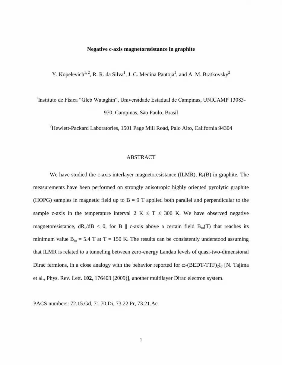
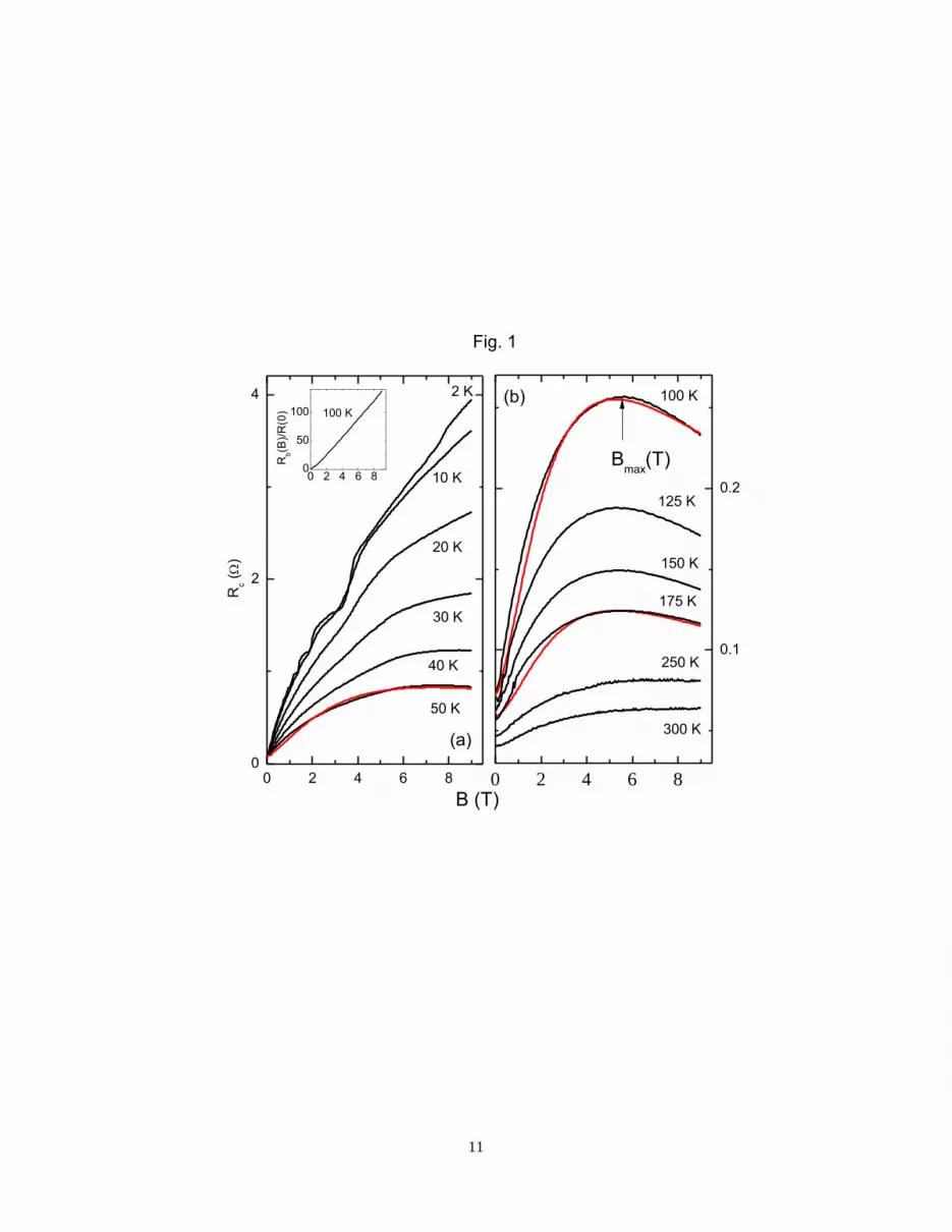
Figure 1 (a, b) presents Rc(B) isotherms recorded for various temperatures. The salient

feature of the data, i. e. the maxima in Rc(B), is indicated by arrows. The negative

magnetoresistance (dRc/dB < 0) reveals itself at B > Bm(T). As shown in Fig. 2, Bm(T) is a non-

monotonic function having the minimum at T ~ 150 K.

4

Taking into account that the basal-plane MR in well graphitized samples is positive and

very big [1], see also the inset in Fig. 1(a), the occurrence of negative MR in the certain domain

of the B-T plane (Fig. 2) should be specific to the c-axis transport. In order to clarify its origin,

we first turn our attention to the zero-field anisotropic electrical transport.

Figure 3 presents normalized c(T) and b(T) resistivity curves obtained for B = 0. As

can be seen from Fig. 3, c(T) demonstrates insulating-like (dc/dT < 0) behavior for T > 50 K,

whereas b(T) rapidly decreases for T < 150 K (db/dT > 0). As a result, the anisotropy c/b

increases as the temperature decreases (see the inset in Fig. 3), representing the characteristic

feature of most anisotropic HOPG. The ratio c/b vs. T can be best fitted by the equation:

c/b = a + bT-

, (1)

where = 0.5. The insulating-type c(T) is the inherent property of a disorder-free graphite, but

the presence of lattice defects can act as short-circuits between the graphene planes, reducing the

measured c(T) compared to its true value [1]. Recent theoretical studies of the perpendicular

transport in graphene multi-layers [14] led to similar conclusions: (i) the perpendicular transport

is enhanced by structural disorder; (ii) the cleaner the system the larger the anisotropy; (iii) the

resistivity ratio c/b ~ T-

at the Dirac point, and diverges when T 0. However, the saturation

of c/b with the temperature lowering is expected for finite doping (chemical potential), being in

agreement with our observations (see the inset in Fig. 3). The predicted exponent = 0.66(6) is

also close to the experimental value = 0.5 found in the present work.

Because of the structural disorder, the current in the measurements flows not only

perpendicular but also parallel to graphene planes. This explains the occurrence of SdH

5

oscillations in the B || I || c configuration, clearly seen for T = 2 K and T = 10 K in Fig. 1(a), top

curve, as well as the metallic-like behavior of Rc(T) at T < 50 K (Fig. 3): both effects are likely

governed by Rb(T).

Then, the resistance measured along the c-axis can be described by the equation for two

parallel resistors Reff = RcRb/(Rc+Rb), where Rb(B) = R0 + aBs(T)

[1, 15] and

Rc(B) = A/(B + B0), (2)

predicted for multilayer DF systems [11, 12], where A and B0 are fitting parameters. The

background physics behind the decreasing Rc vs. B (NILMR) is the Dirac-type Landau level

quantization En = (2evF2|n|B)

1/2 [2], where the lowest Landau level is located precisely at E0 =

0 (zero mode). This has an important consequence: when the interlayer transport is governed by

the tunneling between zero-energy Landau levels, the increase of zero-mode degeneracy with the

field leads to NILMR [11, 12]. Red lines in Fig. 1 are obtained from the equation for Reff(B)

exemplifying good agreement with the experimental results. Somewhat similar interpretation of

the field-driven crossover from positive to negative MR has recently been proposed in the

context of -(BEDT-TTF)2I3 [16], assuming a non-vertical interlayer tunneling. According to

Ref. [16], the crossover field Bm that marks a maximum in Rc(B) corresponds to the crossover

from the inter-Landau level mixing regime (B Bm) to the interlayer tunneling regime between

well separated zero-energy Landau levels (B Bm). This implies that for B > Bm, one has E1 - E0

> kBT, , tc where = ħ/ ( is the transport relaxation time) and tc measure the strength of a

quenched disorder and interlayer tunneling, respectively. It is worth noting, that the old SWMC

model for graphite suggests tc ≈ 0.39 eV >> kBT, and at first glance the comparison of our

6

experimental results with the theoretical models [11, 16], where tc < kBT, may not be appropriate.

However, this value of tc is nearly two orders of magnitude larger than the value ~ 5 meV

reported e. g. by Haering and Wallace [17] who pointed out the 2D character of QPs in graphite,

see also Refs. [4, 18]. Also, recent measurements [19] of current-voltage (I-V) characteristics

performed on graphitic mesas suggested the interlayer tunneling of Dirac fermions between

Landau levels. It seems, both energy scales are relevant in graphite which can be viewed as the

stack of alternating “blocks” of strongly and weakly coupled graphene planes [18, 20], so that

the NILMR originates from the tunneling between nearly decoupled graphitic planes. Taking

characteristic (T) for graphite [21], the inequality (E1 - E0)/kB[K] ≈ ±420|n|1/2

(B[T])1/2

> {T, }

is satisfied over the whole NILMR domain on the B-T plane in Fig. 2.

From this perspective, one also understands the non-monotonic Bm(T). As the

temperature decreases from 300 K to ~ 100 K, the condition E1 - E0 > {kBT, } improves and

hence Bm decreases. At the same time, the inequality tc < kBT inevitably inverts as T 0,

implying the divergence of Bm with the temperature lowering as Fig. 2 illustrates. Assuming that

the minimum in Bm(T) corresponds to the condition tc kBT, one gets tc ~ 10 meV, close to the

value obtained in Ref. [17].

Testing further the theoretical model for NILMR [11], we performed Rc(B)

measurements with B || basal planes (Fig. 4). As Fig. 4 illustrates, in this geometry the negative

MR does not occur for all studied temperatures and magnetic fields, providing evidence that

NILMR is indeed associated with the field component perpendicular to basal planes.

Summarizing, we report the first observation of negative interlayer magnetoresistance

(NILMR) in strongly anisotropic highly ordered graphite that can be consistently understood

within a framework of tunneling models between zero-energy Landau levels of quasi-two-

7

dimensional Dirac fermions [11, 16]. This finding together with the zero-field resistivity

anisotropy measurements, performed in this work, provides an additional experimental evidence

that graphite consists (at least partially ) of weakly coupled graphene planes with the Dirac-type

quasiparticle spectrum.

This work was partially supported by FAPESP, CNPq, and INCT NAMITEC.

8

REFERENCES

[1] B. T. Kelly, Physics of Graphite, Applied Science, London 1981, p. 294.

[2] V. P. Gusynin and S. G. Sharapov, Phys. Rev. Lett. 95, 146801 (2005).

[3] W. W. Toy, M. S. Dresselhaus, and G. Dresselhaus, Phys. Rev. B 15, 4077 (1977).

[4] I. A. Luk’yanchuk and Y. Kopelevich, Phys. Rev. Lett. 93, 166402 (2004).

[5] S.Y. Zhou, G.-H. Gweon, J. Graf, A. V. Fedorov, C. D. Spataru, R. D. Diehl, Y. Kopelevich,

D.-H. Lee, Steven G. Louie, and A. Lanzara et al., Nature Phys. 2, 595 (2006).

[6] G. Li and E. Y. Andrei, Nature Phys. 3, 623 (2007).

[7] M. Orlita, C. Faugeras, G. Martinez, D. K. Maude, M. L. Sadowski, and M. Potemski, Phys.

Rev. Lett. 100, 136403 (2008).

[8] I. A. Luk´yanchuk, Y. Kopelevich, and M. El Marssi, Physica B 404, 404 (2009).

[9] G. Li, A. Luican, and E. Y. Andrei, Phys. Rev. Lett. 102, 176804 (2009)

[10] P. Neugebauer, M. Orlita, C. Faugeras, A. L. Barra and M. Potemski, Phys. Rev. Lett. 103,

136403 (2009).

[11] T. Osada, J. Phys. Soc. Jpn. 77, 084711 (2008).

[12] N. Tajima, S. Sugawara, R. Kato, Y. Nishio, and K. Kajita, Phys. Rev. Lett. 102, 176403

(2009).

[13] Y. Kopelevich, J. H. S. Torres, R. R. da Silva, F. Mrowka, H. Kempa, and P. Esquinazi,

Phys. Rev. Lett. 90, 156402 (2003).

[14] J. Nilsson, A. H. Castro Neto, F. Guinea, and N. M. R. Peres, Phys. Rev. Lett. 97, 266801

(2006).

[15] Y. Kopelevich et al. Phys. Rev. B 73, 165128 (2006).

9

[16] T. Morinari and T. Tohyama, arXiv:0912.0566 [cond-mat. mtrl-sci].

[17] R. R. Hearing and P. R. Wallace, J. Phys. Chem. Solids 3, 253 (1957).

[18] Y. Kopelevich, P. Esquinazi, J. H. S. Torres, R. R. da Silva, and H. Kempa, Adv. Solid

State Phys. 43, 207 (2003); Y. Kopelevich and P. Esquinazi, Adv. Mater. 19, 4559 (2007).

[19] Yu. I. Latyshev, Z. Ya. Kosakovskaya, A. P. Orlov, A.Yu. Latyshev, V.V. Kolesov, P.

Monceau, and D. Vignolles, Journal of Physics: Conference Series 129 , 012032 (2008) .

[20] I. A. Luk’yanchuk and Y. Kopelevich, Phys. Rev. Lett. 97, 256801 (2006).

[21] L. C. Olsen, Phys. Rev. B 6, 4836 (1972).

10

FIGURE CAPTIONS

Fig.1. (Color online) Rc(B) isotherms recorded for various temperatures. The negative

magnetoresistance (dRc/dB < 0) takes place for B > Bm(T) indicated by arrow. Red lines are

obtained from the equation Reff = RcRb/(Rc+Rb), where Rb(B) = R0 + aBs(T)

is the basal-plane

resistance contribution (see text) and Rc(B) = A/(B + B0) with R0, a, A, and B0 being fitting

parameters: R0 = 0.15 , a = 0.26 ·T-1.27

, A = 19 ·T, B0 = 10 T, s = 1.3 (T = 50 K); R0 =

0.085 , a = 0.1 ·T-1.5

, A = 4.85 ·T, B0 = 10 T, s = 1.5 (T = 100 K); R0 = 0.08 , a = 0.04

·T-1.6

, A = 2.5 ·T, B0 = 11 T, s = 1.6 (T = 175 K). The inset in (a) exemplifies Rb(B)/Rb(0)

measured with the current flowing parallel to basal graphitic planes.

Fig.2. Bm(T) separates positive (dRc/dB > 0) and negative (dRc/dB < 0) magnetoresistance.

Fig.3. (Color online) Normalized c-axis c(T)/c(300 K) and basal-plane b(T)/b(300 K)

resistivity curves obtained for B = 0. The inset presents the anisotropy c/b vs. T; the red line is

obtained from Eq. (1): a = 1.1, b = 40 K, = 0.5.

Fig.4. Rc(B) measured at various temperatures and B || basal planes.

11

0 2 4 6 80

2

4

0 2 4 6 8

0.1

0.20 2 4 6 8

0

50

100

Rc (

)

2 K

10 K

20 K

30 K

40 K

50 K

(a)

B (T)

100 K

125 K

150 K

175 K

250 K

300 K

(b)

Bmax

(T)

Fig. 1

Rb(B

)/R

(0) 100 K

12

50 100 150 200 250 3005

6

7

8

NEGATIVE

MAGNETORESISTANCE

Bm (

T)

T (K)

Fig. 2

13

0 50 100 150 200 250 300

0.5

1.0

1.5

2.0

5

10

15

b(T)

(T

)/

(30

0 K

)

T (K)

B = 0c(T)

Fig. 3

10

-4

c/

b

c/

b = a +bT

-

14

0 2 4 6 8 100.0

0.2

0.4

0.6

0.8

1.0

20 K

Rc (

)

B (T)

Fig. 4

T = 2 K

B || basal planes

10 K

30 K

40 K

50 K

70 K

100 K150 K200 K250 K