Embed Size (px)
Citation preview

New York State
Economic, Revenue and Spending Methodologies
Eliot Spitzer, Governor Paul E. Francis, Director of the Budget and Senior Advisor to the Governor October 31, 2007

Table of Contents
Overview of the Methodology Process ........................................... 1
Part I - Economic Methodologies Macroeconomic Model ................................................................ 13 New York State Macroeconomic Model ...................................... 45 New York State Adjusted Gross Income..................................... 53
Part II - Revenue Methodologies Personal Income Tax .................................................................. 67 User Taxes and Fees
Sales and Use Tax ................................................................. 89 Cigarette and Tobacco Taxes ................................................ 98 Motor Fuel Tax ....................................................................... 106 Motor Vehicle Fees................................................................. 112 Alcoholic Beverage Taxes and Alcoholic Beverage
Control License Fees ......................................................... 116 Highway Use Tax ................................................................... 124
Business Taxes Bank Tax ................................................................................ 129 Corporate Franchise Tax........................................................ 138 Corporation and Utilities Taxes............................................... 152 Insurance Taxes ..................................................................... 159 Petroleum Business Taxes..................................................... 170
Other Taxes Estate Tax .............................................................................. 178 Real Estate Transfer Tax........................................................ 186 Pari-Mutuel Taxes .................................................................. 192
Lottery ......................................................................................... 198 Video Lottery ............................................................................... 212
Part III - Spending Methodologies School Aid ................................................................................... 227 Medicaid...................................................................................... 233 Welfare........................................................................................ 243 Child Welfare............................................................................... 249 Debt Service................................................................................ 252 Personal Service ......................................................................... 261 Non-Personal Service ................................................................. 269 Employee Health Insurance ........................................................ 278 Pensions ..................................................................................... 282
1
AN OVERVIEW OF THE METHODOLOGY PROCESS
The Division of the Budget (DOB) Economic, Revenue and Spending Methodologies supplements the detailed forecast of the economy, tax, and spending forecasts presented in the Executive Budget and Quarterly Updates. The purpose of this volume is to provide background information on the methods and models used to generate the estimates for the major receipt and spending sources contained in the 2007-08 Mid-Year Update and the upcoming 2008-09 Executive Budget. DOB’s forecast methodology utilizes sophisticated econometric models, augmented by the input of a panel of economic experts, and a thorough review of economic, revenue and spending data to form multi-year quarterly projections of economic, revenue and spending changes. The major innovation in this edition of the Methodology is the inclusion of a detailed discussion of spending methodologies. This addition is part of a continued effort to promote transparency in the Budget process. The new sections comply with provisions in Budget Reform Legislation passed in 2007. The spending side analysis is designed to provide, in summary form, background information on the methods and analyses used to generate the spending estimates for a number of major program areas contained in the budget, and is meant to enhance the presentation and transparency of the State's spending forecast. The methodologies illustrate how spending forecasts are the product of many factors and sources of information, including past performance and trends, administrative constraints, expert judgment of agency staff, and information in the State's economic analysis and forecast, especially where spending trends are sensitive to changes in economic conditions. AN ASSESSMENT OF FORECAST RISK No matter how sophisticated the methods used, all forecasts are subject to error. For this reason, a proper assessment of the most significant forecast risks can be as critical to the budget process as the forecast itself. Therefore, we begin by reviewing the most important sources of forecast error and discuss how they affect the spending and receipt forecasts used to construct the Mid-Year Update. Data Quality Even the most accurate forecasting model is constrained by the accuracy of the available data. The data used by the Budget Division to produce a forecast typically undergo several stages of revision. For example, the quarterly components of real U.S. gross domestic product (GDP), the most widely cited measure of national economic activity, are revised no less than five times over a four-year period, not including the rebasing process. Each revision incorporates data that were not available when the prior estimate was made. Initial estimates are often based on sample information, though early vintages are sometimes based on the informed judgment of the analyst charged with tabulating the data. The monthly employment estimates produced under the Current Employment

AN OVERVIEW OF THE FORECAST PROCESS
2
Statistics (CES) program undergo a similar revision process as better, more broad-based data become available and with the evolution of seasonal factors. The total U.S. nonagricultural employment estimate for December 1989 has been revised no less than ten times since it was first published in January 1990.1 Less frequently, data are revised based on new definitions of the underlying concepts.2 Unfortunately, revisions tend to be largest at or near business cycle turning points, when accuracy is most critical to fiscal planners. Finally, as demonstrated below, the available data are sometimes not suitable for economic or revenue forecasting purposes, such as the U.S. Bureau of Economic Analysis’ estimate of wages at the state level. Model Specification Error Economic forecasting models are by necessity simplifications of complex social processes involving millions of decisions made by independent agents. Although economic and fiscal policy theory provide some guidance as to how these models should be specified, theory is often imprecise with respect to capturing behavioral dynamics and structural shifts. Moreover, modeled relationships may vary over time. Often one must choose between models that use the average behavior of the series over its entire history to forecast the future and models which give more weight to the more recent behavior of the series. Although more complicated models may do a better job of capturing history, they may be no better at forecasting the future, leading to the parsimony principle as a guiding precept in the model building process. Model Coefficients: Fixed Points or Ranges? Although model coefficients are generally treated as fixed in the forecasting process, coefficient estimates are themselves random variables, governed by probability distributions. Typically, the error distribution is assumed to be normal, a key to making statistical inference. Reporting the standard errors of the coefficient distributions gives some indication of the precision with which one can measure the relationship between two variables. For many of the results reported below, point estimates of the coefficients are reported along with their standard errors or t-statistics. However, it would be more accurate to say that there is a 66 percent probability that the true coefficient lies within a range of the estimated coefficient plus and minus the standard error. Economic Shocks A multitude of random events occur that can affect the economy, and by association spending and revenue results, but that no model can adequately capture. September 11 is the most extreme example of such an event. Some economic variables are more sensitive to shocks than others. For example, equity markets rise and fall on the day’s news, sometimes by large magnitudes. 1 The current estimate for total employment for December 1989 of 108.8 million is 0.7 percent below the initial estimate of 109.5. 2 The switch from SIC to NAICS, classification concepts is a classic example of how changes in the definition of a data series can challenge the modeler. The switch not only changed the industrial classification scheme, but also robbed state modelers of decades of employment history.
AN OVERVIEW OF THE FORECAST PROCESS
3
In contrast, GDP growth tends to fluctuate within a relatively narrow range. For all of these reasons, the probability of any forecast being precisely accurate is virtually zero. But although one can not be confident about hitting any particular number correctly, one can feel more confident about specifying a range within which the actual number is likely to fall. Often economic forecasters use sophisticated techniques, such as Monte Carlo analysis, to estimate confidence bands based on the model’s performance, the precision of the coefficient estimates, and the inherent volatility of the series. A 95 percent confidence band (or even a much less exacting band) often can be quite wide, suggesting the possibility that the actual result could deviate substantially from the point estimate. From a practitioner’s perspective, these techniques are only valid if the model is properly specified. What sometimes appears to be a random economic shock may actually be a more permanent structural change. Structural shifts in the underlying economy, revenue or spending structure are difficult to model in practice, particularly since the true causes of such shifts only become clear with hindsight. This can lead to large forecast errors when these shifts occur rapidly or when the cumulative impact is felt over the forecast horizon. Policy makers must be kept aware that even a well specified model can perform badly when structural changes occur. Evaluating a Loss Function The prevalence of sources of forecast error underscores the importance of assessing the risks to the forecast, and explains why the discussion of such risks consumes such a large portion of the economic backdrop presented with the Executive Budget. In light of all of the potential sources of forecast risk, how does a budgeting entity utilize the knowledge of risks to inform the forecast? Standard econometric theory tells us that the probability of any point forecast being correct is virtually zero, but a budget must be based on a single projection. One way to reconcile these two facts is to evaluate the cost of one’s forecasting errors, giving rise to the notion of a loss function. A conventional example of a loss function is the root-mean-squared forecast error (RMSFE). In constructing that measure, the “cost” of an inaccurate forecast is the square of the forecast error itself, implying that large forecast errors are weighted more heavily than small errors. Because positive and negative errors of equal magnitude are weighted the same, the RMSFE is symmetric. However, in the professional world of forecasting, as in our daily lives, the costs associated with an inaccurate forecast may not truly be symmetric. For example, how much time we give ourselves to get to the airport may not be based on the average travel time between home and the gate, since the cost of being late and missing the plane may outweigh the cost of arriving early and waiting awhile longer. Granger and Pesaran (2000) show that the forecast evaluation criterion derived from their decision-based approach can differ markedly from the usual RMSFE. They suggest a more general approach, known as generalized cost-of-error functions,
AN OVERVIEW OF THE FORECAST PROCESS
4
to deal with asymmetries in the cost of over- and under-predicting.3 In the revenue-estimating context, the cost of overestimating receipts for a fiscal year may outweigh the cost of underestimating receipts, given that ongoing spending decisions may be based on revenue resources projected to be available. In summary, forecast errors are an inevitable part of the process and, as a result, policymakers must be fully informed of the forecast risks, both as to direction and magnitude.
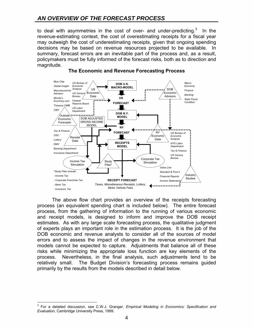
The Economic and Revenue Forecasting Process
Tax & Finance
OSC
Lottery
DMV
Banking Department
Insurance Department
Macro Economy
Finance
Banking
State Fiscal Condition
RECEIPT FORECAST
DOB U.S.MACRO-MODEL
OutsideEconomicForecasts
DOBEconomicAdvisors
DOB N.Y.MODEL
US
FORECAST
NY
FORECAST
Income TaxSimulation
Corporate TaxSimulation
ReceiptData
Value Line
Standard & Poor’s
Financial Reports
Income Statements
RECEIPTSMODEL
StudyFiles*
*Study Files Include:
- Income Tax
- Corporate Franchise Tax
- Bank Tax
- Insurance Tax
Taxes, Miscellaneous Receipts, Lottery, Motor Vehicle Fees
DOB ADJUSTEDGROSS INCOME
MODEL
IndustryStudies
NYEconomic
Data
US Bureau of Economic Analysis
NYS Labor Department
Tax & Finance
US Census Bureau
USEconomic
Data
US Bureau of Economic Analysis
US Census Bureau
Federal Reserve Board
US Labor Department
Blue Chip
Global Insight
Macroeconomic Advisers
Moody’s Economy.com
Treasury OMB
CBO
The above flow chart provides an overview of the receipts forecasting process (an equivalent spending chart is included below). The entire forecast process, from the gathering of information to the running of various economic and receipt models, is designed to inform and improve the DOB receipt estimates. As with any large scale forecasting process, the qualitative judgment of experts plays an important role in the estimation process. It is the job of the DOB economic and revenue analysts to consider all of the sources of model errors and to assess the impact of changes in the revenue environment that models cannot be expected to capture. Adjustments that balance all of these risks while minimizing the appropriate loss function are key elements of the process. Nevertheless, in the final analysis, such adjustments tend to be relatively small. The Budget Division’s forecasting process remains guided primarily by the results from the models described in detail below.
3 For a detailed discussion, see C.W.J. Granger, Empirical Modeling in Economics: Specification and Evaluation, Cambridge University Press, 1999.
AN OVERVIEW OF THE FORECAST PROCESS
5
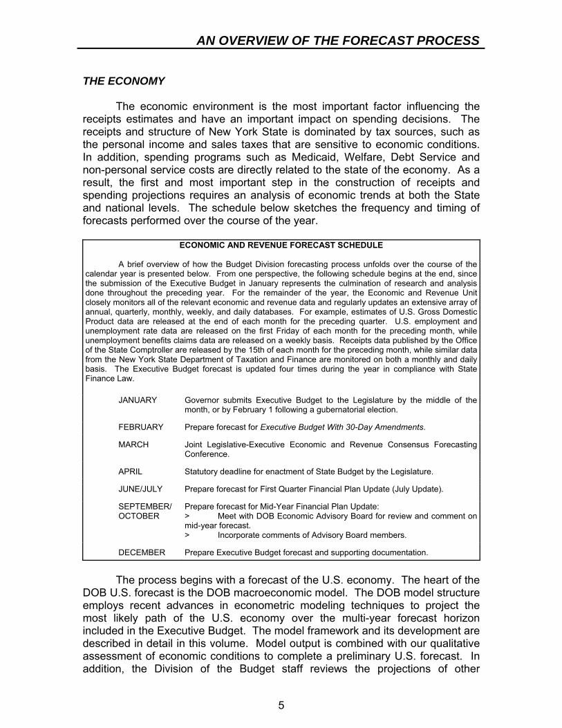
THE ECONOMY The economic environment is the most important factor influencing the receipts estimates and have an important impact on spending decisions. The receipts and structure of New York State is dominated by tax sources, such as the personal income and sales taxes that are sensitive to economic conditions. In addition, spending programs such as Medicaid, Welfare, Debt Service and non-personal service costs are directly related to the state of the economy. As a result, the first and most important step in the construction of receipts and spending projections requires an analysis of economic trends at both the State and national levels. The schedule below sketches the frequency and timing of forecasts performed over the course of the year.
ECONOMIC AND REVENUE FORECAST SCHEDULE A brief overview of how the Budget Division forecasting process unfolds over the course of the calendar year is presented below. From one perspective, the following schedule begins at the end, since the submission of the Executive Budget in January represents the culmination of research and analysis done throughout the preceding year. For the remainder of the year, the Economic and Revenue Unit closely monitors all of the relevant economic and revenue data and regularly updates an extensive array of annual, quarterly, monthly, weekly, and daily databases. For example, estimates of U.S. Gross Domestic Product data are released at the end of each month for the preceding quarter. U.S. employment and unemployment rate data are released on the first Friday of each month for the preceding month, while unemployment benefits claims data are released on a weekly basis. Receipts data published by the Office of the State Comptroller are released by the 15th of each month for the preceding month, while similar data from the New York State Department of Taxation and Finance are monitored on both a monthly and daily basis. The Executive Budget forecast is updated four times during the year in compliance with State Finance Law. JANUARY Governor submits Executive Budget to the Legislature by the middle of the
month, or by February 1 following a gubernatorial election.
FEBRUARY Prepare forecast for Executive Budget With 30-Day Amendments.
MARCH Joint Legislative-Executive Economic and Revenue Consensus Forecasting Conference.
APRIL Statutory deadline for enactment of State Budget by the Legislature.
JUNE/JULY Prepare forecast for First Quarter Financial Plan Update (July Update).
SEPTEMBER/ OCTOBER
Prepare forecast for Mid-Year Financial Plan Update: > Meet with DOB Economic Advisory Board for review and comment on mid-year forecast. > Incorporate comments of Advisory Board members.
DECEMBER Prepare Executive Budget forecast and supporting documentation.
The process begins with a forecast of the U.S. economy. The heart of the DOB U.S. forecast is the DOB macroeconomic model. The DOB model structure employs recent advances in econometric modeling techniques to project the most likely path of the U.S. economy over the multi-year forecast horizon included in the Executive Budget. The model framework and its development are described in detail in this volume. Model output is combined with our qualitative assessment of economic conditions to complete a preliminary U.S. forecast. In addition, the Division of the Budget staff reviews the projections of other
AN OVERVIEW OF THE FORECAST PROCESS
6
forecasters of the U.S. economy to provide a yardstick against which to judge the DOB forecast. The U.S. forecast serves as the key input to the New York macroeconomic forecast model. National conditions with respect to employment, income, financial markets, foreign trade, consumer confidence, and stock market prices can have a major impact on New York’s economic performance. However, the New York economy is subject to idiosyncratic fluctuations, which can lead the State economy to perform much differently than the nation as a whole. The evolution of the New York economy is governed in part by a heavy concentration of jobs and income in the financial and business service industries. As a result, economic events that disproportionately affect these industries can have a greater impact on the New York economy than on the rest of the nation. The New York economic model is structured to capture both the obvious linkages to the national economy and the factors which may cause New York to deviate from the nation. The model estimates the future path of major elements of the New York economy, including employment, wages and other components of personal income and makes explicit use of the linkages between employment and income earned in the financial services sector and the rest of the State economy. To adequately forecast personal income tax receipts — the largest single component of the receipts base — projections of the income components that make up State taxable income are also required. For this purpose, DOB has constructed models for each of the components of New York State adjusted gross income. The results from this series of models serve as input to the income tax simulation model described below, which is the primary tool for calculating New York personal income tax liability. A final part of the economic forecast process involves using tax collection data to assess the current state of the New York economy. Tax data are often the most current information available for judging economic conditions. For example, personal income tax withholding provides information on wage and employment growth, while sales tax collections serve as an indicator of consumer purchasing activity. Clearly, there are dangers in relying too heavily on tax information to forecast the economy, but these data are vital in assessing the plausibility of the existing economic forecast, particularly for the year in progress and at or near turning points when “realtime” data are most valuable. ECONOMIC ADVISORY BOARD At this point, a key component of the forecast process takes place: the Budget Director and staff confer with a panel of economists with expertise in macroeconomic forecasting, finance, the regional economy, and public sector economics to obtain valuable input on current and projected economic conditions, as well as an assessment of the reasonableness of the DOB estimates of revenue and spending. In addition, the panel provides input on other key functions that may impact receipts growth, including financial services
AN OVERVIEW OF THE FORECAST PROCESS
7
compensation and the performance of sectors of the economy difficult to capture in any model. FORECASTING RECEIPTS Once the economic forecast is complete, these projections are used to forecast selected revenues. Again, DOB combines qualitative assessments, the econometric analysis, and expert opinions on the New York revenue structure to produce a final receipts forecast. Decomposing Cash collections Much can be learned about the forces operating on receipts just by carefully examining the data. Many of the revenue sections of this report contain a series of related plots termed “component collection graphs.” The first graph in the series is the raw collections data for the tax. The next three plot the underlying components of the series as determined by the structural time series approach developed by Harvey. This approach decomposes the series into its trend, seasonal, and irregular components. In many cases, close examination of these charts reveals important patterns and shifts in the data that suggest strategies for modeling and forecasting. Although these graphs are not a substitute for more substantive analysis, they represent a productive first step in evaluating the data-generating process. Modeling and Forecasting The DOB receipts estimates for the major tax sources rely on a sophisticated set of econometric models that link economic conditions to revenue-generating capacity. The models use the economic forecasts described above as inputs and are calibrated to capture the impact of policy changes. As part of the revenue estimating process, DOB staff analyze industry trends, tax collection experience, and other information necessary to better understand and predict receipts activity. For large tax sources, such as the personal income tax, receipt estimates are approached by constructing underlying taxpayer liability and then projecting liability into future periods based on the economic forecast generated from econometric models specifically developed for each tax. After liability is estimated for future taxable periods, it is converted to cash estimates on a fiscal year basis. The Division of the Budget employs microsimulation models to estimate future tax liabilities for the personal income and corporate business taxes. This technique starts with detailed taxpayer information taken directly from tax returns (the data are stripped of identifying taxpayer information) and allows for the actual computation of tax under alternative policy and economic scenarios. Microsimulation allows for a bottom-up estimate of tax liability for future years as the data file of taxpayers is “grown,” based on DOB estimates of economic growth. An advantage of this approach is that it allows direct calculation of tax
AN OVERVIEW OF THE FORECAST PROCESS
8
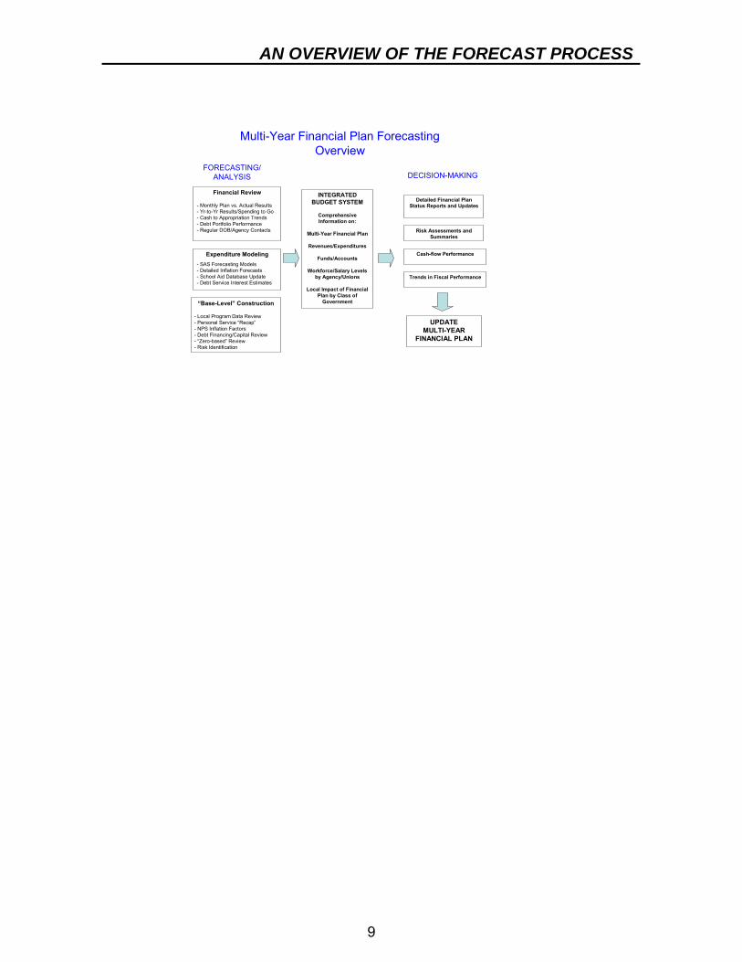
law changes and the revenue impact of already enacted and proposed tax changes on future liability. As with most DOB revenue models, the simulation models require projections of the economic variables that drive tax liability. The personal income tax and corporate business tax simulation models incorporate the direct effect of a policy change on taxpayers. However, the models do not permit feedback from the taxpayer back to the macroeconomy. For large policy changes intended to influence taxpayer behavior and trigger changes in the underlying economy, adjustments are made outside the modeling process.4 Simulating future tax liability is most important for the personal income tax, which accounts for over half of General Fund tax receipts and is discussed in greater detail later in this report. FORECASTING SPENDING This version of the Budget Methodology includes a new detailed section on methods used to predict the major components of State spending. Like the revenue forecasts, the spending projections are often closely tied to the DOB economic forecast. In other cases, just as is the case for receipts, the spending projections are tied closely to the institutional and demographic factors specific to a spending program. Each spending methodology addresses at least four key components, including an overview of important program concepts, a description of relationships between variables and how this relates to the spending forecast, how the forecasts translate into the current Financial Plan estimates, and the risks and variations inherent in the forecast. These factors are described in more detail below for key program areas that drive roughly 80 percent of the State's overall spending forecast. The following chart depicts, in broad terms, the multi-year forecasting process that DOB employs in constructing its spending forecasts.
4 For examples of modeling efforts that attempt to incorporate such feedback, see Congressional Budget Office, How CBO Analyzed the Macroeconomic Effects of the President's Budget, July 2003.
AN OVERVIEW OF THE FORECAST PROCESS
9
Multi-Year Financial Plan Forecasting Overview
Financial Review
- Monthly Plan vs. Actual Results- Yr-to-Yr Results/Spending to Go- Cash to Appropriation Trends- Debt Portfolio Performance- Regular DOB/Agency Contacts
“Base-Level” Construction
- Local Program Data Review - Personal Service “Recap”- NPS Inflation Factors - Debt Financing/Capital Review- “Zero-based” Review - Risk Identification
Expenditure Modeling- SAS Forecasting Models - Detailed Inflation Forecasts - School Aid Database Update - Debt Service Interest Estimates
UPDATE MULTI-YEAR
FINANCIAL PLAN
FORECASTING/ ANALYSIS DECISION-MAKING
INTEGRATED BUDGET SYSTEM
Comprehensive Information on:
Multi-Year Financial Plan
Revenues/Expenditures
Funds/Accounts
Workforce/Salary Levels by Agency/Unions
Local Impact of Financial Plan by Class of
Government
Detailed Financial Plan Status Reports and Updates
Risk Assessments and Summaries
Cash-flow Performance
Trends in Fiscal Performance


11
Part I - Economic Methodologies


13
U.S. MACROECONOMIC MODEL The Division of the Budget (DOB) Economic and Revenue Unit provides projections on a wide range of economic and demographic variables. These estimates are used in the development of revenue and expenditure projections for the State, debt capacity analysis, and for other budget planning purposes. The Division has developed econometric models for the U.S. and State economies that yield the forecasts needed for these purposes. RECENT DEVELOPMENTS IN MACROECONOMIC MODELING Macroeconomic modeling has undergone a number of important changes during the last 25 years, primarily as a result of developments in economic and econometric theory. However, fundamental changes in the structure of the economy since the 1970s have also led to a significant altering of the way the economy is modeled. The Budget Division macroeconomic model for the U.S. economy incorporates four related lines of economic research that have had a significant impact on macroeconomic modeling. The first major development was Robert Lucas’ (1976) critique of the role of expectations in traditional macroeconomic models. If economic models did not incorporate the assumption that agents were forward looking, then it would be unlikely that model forecasts would be consistent with a rational response on the part of agents to a possible policy change. The result was a widespread adoption of rational expectations in macroeconomic forecasting models. The Lucas analysis also initiated the emergence of a new generation of econometric models explicitly based on micro-foundations in which firms and households are assumed to make decisions based on optimization plans that are realized in the long run. Second, Christopher Sims (1980) raised serious doubts that standard large-scale econometric models were effective in properly identifying the behavioral relations among agents in the economy. This critique led to a more flexible identification of the behavioral relations among economic agents within a vector autoregression (VAR) model framework. Unlike structural models, VAR models do not impose an a priori structure on the dynamic relationships among economic variables. A third development was initiated by the classic study of Nelson and Plosser (1982), which concluded that the hypothesis of nonstationarity cannot be rejected for a wide range of commonly used macroeconomic data series. Heuristically, nonstationarity implies the lack of a constant mean and variance in a time series. Research surrounding the absence of stationarity led to a re-evaluation of what constitutes a long-run equilibrium relationship, and prompted a revisiting of the problem of spurious regression described by Granger and Newbold (1974). This led to a more rigorous analysis of the time series properties of economic data and the implications of these properties for model specification and statistical inference.
US MACROECONOMIC MODEL
14
Further, nonstationarity also led to a fourth development, engendered by the work of Engle and Granger (1987), Johansen (1991), and Phillips (1991) on the presence of long-run equilibrium relationships among macroeconomic data series, also known as cointegration. Although cointegrated series can deviate from their long-term trends for substantial periods, there is always a tendency to return to their common equilibrium paths. This behavior led to the development of a framework for dealing with nonstationary data in an econometric setting known as the error-correction model. The error-correction framework has permitted extensive research on how to best exploit the predictive power of cointegrating relationships. Another area that has spawned a substantial wealth of academic research is the choice of an optimal monetary policy. The dramatic changes in the institutional structure of financial markets over the past 25 years have rendered the aggregate money supply a much less tractable target than interest rates. In addition, new developments in economic theory, including game theory and the rational expectations hypothesis, appear to favor a rule-based monetary policy, as opposed to a purely discretionary approach. A rule-based approach is believed to maximize the credibility of the central bank, a key input to the effectiveness of the policy itself. However, the desirability of this feature must be weighed against the reliability of the information available when policy decisions are made. Perhaps the most popular example of an interest rate-setting rule is the one proposed by John Taylor (1993), commonly known as Taylor’s rule. According to Taylor’s rule, the monetary authority’s policy choices are guided by the extent to which inflation and output deviate from target levels, though the debate as to precisely how the rule should be specified is ongoing. Recent research by Orphanides (2003) using real-time data indicates that Federal Reserve policy has been consistent with a “Taylor-rule framework” almost since its inception. However, there is mounting empirical evidence that the Federal Reserve has more vigorously pursued a policy of keeping inflation expectations well anchored since the early 1980s. This evidence suggests that a policy rule which augments actual inflation by expectations may be optimal. BASIC FEATURES The Division of the Budget’s U.S. macroeconomic model (DOB/U.S.) incorporates the theoretical advances described above in an econometric model used for forecasting and policy simulation. The agents represented by the model’s behavioral equations optimize their behavior subject to economically meaningful constraints. The model addresses the Lucas critique by specifying an information set that is common to all economic agents, who incorporate this information when forming their expectations. The model’s long-run equilibrium is the solution to a dynamic optimization problem carried out by households and firms. The model structure incorporates an error-correction framework that ensures movement back to equilibrium in the long run. Like the Federal Reserve Board model summarized in Brayton and Tinsley (1996), the assumptions that govern the long-run behavior of DOB/U.S.
US MACROECONOMIC MODEL
15
are grounded in neoclassical microeconomic foundations. Consumers exhibit maximizing behavior over consumption and labor-supply decisions, while firms maximize profit. The model solution converges to a balanced growth path in the long run. Consumption is determined by expected wealth, which is determined, in part, by expected future output and interest rates. The value of investment is affected by the cost of capital and expectations about the future path of output and inflation. However, in addition to the microeconomic foundations which govern long-run behavior, DOB/U.S. incorporates dynamic adjustment mechanisms, reflecting that even forward-looking agents do not adjust instantaneously to changes in economic conditions. Sources of “friction” within the economy include adjustment costs, the wage-setting process, and persistent spending habits among consumers. Frictions delay the adjustment of nonfinancial variables, producing periods when labor and capital deviate from their optimal paths. The presence of such imbalances constitutes signals that are important in the setting of wages and prices because price setters must anticipate the actions of other agents. For example, firms set wages and prices in response to a set of expectations concerning productivity growth, available labor, and the consumption choices of households. In contrast to the “real” sector, the financial sector is assumed to be unaffected by frictions due to the negligible cost of transactions and the presence of well developed primary and secondary markets for financial assets. This contrast between the real and financial sectors permits monetary policy to have a short-run impact on output. Monetary policy is administered through interest rate manipulation via a federal funds rate policy target. Current and anticipated changes in this rate influence agents’ expectations and the rate of return on various financial assets. OVERVIEW OF MODEL STRUCTURE DOB/U.S. comprises six modules of estimating equations, forecasting well over 200 variables. The first module estimates real potential U.S. output, as measured by real U.S. gross domestic product (GDP). The next module estimates the formation of agent expectations, which become inputs to blocks of estimating equations in subsequent modules. Agent expectations play a key role in determining long-term equilibrium values of important economic variables, such as consumption and investment, which are estimated in the third module. A fourth module produces forecasts for variables thought to be influenced primarily by exogenous forces but which, in turn, play an important role in determining the economy’s other major indicators. These variables, along with the long-term equilibrium values estimated in the third module, become inputs to the core behavioral model, which comprises the fifth block of estimating equations. The core behavioral model is the largest part of DOB/U.S. and much of the discussion that follows focuses on this component. The final module is comprised of satellite models that use core model variables as inputs, but do not feed back into the core behavioral equations.
US MACROECONOMIC MODEL
16
The current estimation period for the model is the first quarter of 1965 through the second quarter of 2006, although some data series do not have historical values for the full period.1 Descriptions of each of the six modules follow below. POTENTIAL OUTPUT AND THE OUTPUT GAP Potential Gross Domestic Product (GDP) is one of the foundational elements of DOB/U.S., on which the model's long-term equilibrium values and monetary policy forecasts are based. Potential GDP is the level of output that the economy can produce when all available resources are being utilized at their most efficient levels. The economy can produce both above and below this level, but when it does so for an extended period, economic agents can expect inflation to either rise or fall, respectively, although the precise timing of that movement can depend on a multiplicity of factors. The output gap is defined as the difference between actual and potential output. The Budget Division's method for estimating potential GDP largely follows that of the Congressional Budget Office (CBO) (1995, 2001). This method estimates potential GDP for each of the four major economic sectors defined under U.S. Bureau of Economic Analysis (BEA) National Income and Product Account (NIPA) data: private nonfarm business, private farm, government, and households and nonprofit institutions. The nonfarm business sector is by far the largest sector of the U.S. economy, accounting for 77.4 percent of total GDP in 2000. A neoclassical growth model is used to model this sector, incorporating three inputs to the production process: labor (measured by the number of hours worked), the capital stock, and total factor productivity. The last of these three inputs, total factor productivity, is not directly measurable. It is estimated by substituting the actual values of hours worked and capital into a fixed coefficient Cobb-Douglas production function, where a coefficient of 0.7 is applied to labor and 0.3 is applied to capital; all values are in logarithms. Total factor productivity is the residual resulting from a subtraction of the log value of output accounted for by labor and capital from the historical log value of output. Each of the inputs to private nonfarm business production is assumed to contain a component that varies with the business cycle and a long-term trend component that tracks the evolution of economy's capacity to produce. Inputs are adjusted to their “potential” levels by estimating and then removing the cyclical component from the data series. The cyclical component is assumed to be reflected in the deviation of the actual unemployment rate from what economists define as the nonaccelerating inflation rate of unemployment, or NAIRU. When the unemployment rate falls below the NAIRU, indicating a tight labor market, the stage is set for higher wage growth and, in turn, higher inflation. An unemployment rate above the NAIRU has the opposite effect. Estimation of the long-term trend component presumes that the "potential" level of an input grows smoothly over time, though not necessarily at a fixed growth rate. Once the models are estimated, the potential level is defined as the fitted values from 1 The specific estimation results presented in the tables below are based on data through the third quarter of 2005. The addition of three quarters changes these results only marginally.
US MACROECONOMIC MODEL
17
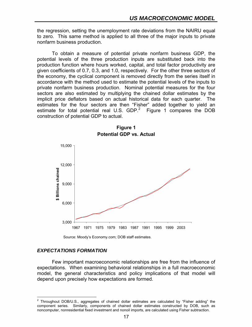
the regression, setting the unemployment rate deviations from the NAIRU equal to zero. This same method is applied to all three of the major inputs to private nonfarm business production. To obtain a measure of potential private nonfarm business GDP, the potential levels of the three production inputs are substituted back into the production function where hours worked, capital, and total factor productivity are given coefficients of 0.7, 0.3, and 1.0, respectively. For the other three sectors of the economy, the cyclical component is removed directly from the series itself in accordance with the method used to estimate the potential levels of the inputs to private nonfarm business production. Nominal potential measures for the four sectors are also estimated by multiplying the chained dollar estimates by the implicit price deflators based on actual historical data for each quarter. The estimates for the four sectors are then “Fisher” added together to yield an estimate for total potential real U.S. GDP.2 Figure 1 compares the DOB construction of potential GDP to actual.
Figure 1
3,000
6,000
9,000
12,000
15,000
1967 1971 1975 1979 1983 1987 1991 1995 1999 2003
$ B
illio
ns c
hain
ed
Potential GDP vs. Actual
Source: Moody’s Economy.com; DOB staff estimates.
EXPECTATIONS FORMATION Few important macroeconomic relationships are free from the influence of expectations. When examining behavioral relationships in a full macroeconomic model, the general characteristics and policy implications of that model will depend upon precisely how expectations are formed.
2 Throughout DOB/U.S., aggregates of chained dollar estimates are calculated by “Fisher adding” the component series. Similarly, components of chained dollar estimates constructed by DOB, such as noncomputer, nonresidential fixed investment and nonoil imports, are calculated using Fisher subtraction.
US MACROECONOMIC MODEL
18
Rational and Adaptive Expectations Expectations play an important role in DOB/U.S. in the determination of consumer and firm behavior. For example, when deciding expenditure levels, consumers will take a long-term view of their wealth prospects. Thus, when deciding how much to spend in a given period, they consider not only their income in that period, but also their lifetime or “permanent income,” as per the “life cycle” or “permanent income” hypotheses put forward by Friedman (1957) and others. In estimating their permanent incomes, consumers are assumed to use all the information available to them at the time they make purchases. Producers are also assumed to be forward-looking, basing their decisions on their expectations of future prices, interest rates, and output. However, since both households and firms experience costs associated with adjusting their long-term expenditure plans, both are assumed to exhibit a degree of behavioral inertia, making adjustments only gradually. DOB/U.S. assumes that all economic agents form their expectations “rationally,” meaning all available information is used, and that expectations are correct, on average, over the long-term. More formally, the expectation of a variable Y at time t, Yt, formed at period t-1, is the statistical expectation of Yt based on all available information at time t-1. However, because of the empirical finding that agents adjust their expectations only gradually, expectations in DOB/U.S. are assumed to have an “adaptive” component as well. Adaptive expectations are captured by including the term, αYt-1, where α is hypothesized to be between zero and one. Consistent with rational expectations theory, it is assumed that agents’ long-run average forecast error is zero. This “hybrid” specification is inspired by Roberts (2001), Rudd and Whelan (2003), Sims (2003), and others who find that the notions of adaptive and rational expectations should not be viewed as mutually exclusive, particularly in light of the high information costs associated with forecasting. Moreover, given the empirical importance of lags in forecasting inflation, as well as other economic variables, it cannot be said that “price-stickiness” is model-inconsistent. While the importance of expectations in forecasting is now well established, their specification continues to challenge model builders. DOB/U.S. estimates agent expectations in two stages. First, measures of expectations pertaining to three key economic variables are estimated within a vector autoregressive framework. These expectations become part of an information set that is shared by all agents who then use them, in turn, to form expectations over variables that are specific to a particular subset of agents, such as households and firms. Details of this process are presented below. Shared Expectations All agents in DOB/U.S. use a common information set to form expectations. This set consists of three key macroeconomic variables: inflation as represented by the GDP price deflator, the percentage output gap, and the federal funds rate. The percentage output gap is defined as actual real GDP minus potential real GDP, divided by actual real GDP. The variables are
US MACROECONOMIC MODEL
19
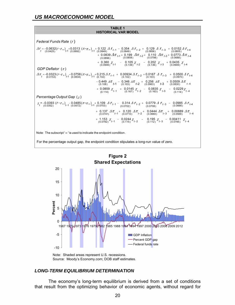
estimated within a VAR framework, with the federal funds rate and the GDP inflation rate in first-difference form (see Table 1). The long-run values of the three variables are constrained by “endpoint” conditions. Two of these restrictions are represented by the first two terms on the right-hand side in Table 1. For inflation, the terminal constraint is the ten-year inflation rate expectation, as measured by survey data developed by the Federal Reserve Bank of Philadelphia. The endpoint condition for the federal funds rate is computed from forward rates. The assumption that the percentage output gap becomes zero in the long run is implied and need not appear explicitly in the equations. An important feature of the endpoint restrictions for the federal funds rate and inflation is that they are not fixed. Should the public alter its expectations in response to economic developments, such as a shift in monetary policy, these changes are captured and then fed into the rest of the model. Figure 2 illustrates how the three variables that comprise shared expectations converge to their long-term equilibrium values over time. Agent-Specific Expectations The common information set is augmented by expectations pertaining to agents in specific sectors. For example, households base their consumption decisions on the expected lifetime accumulation of income and wealth. Therefore, the household-specific information set includes expectations over the components of real disposable personal income and after-tax values of securities- and non-securities-related wealth. Similarly, the firm sector-specific information set includes expectations over the relative prices of investment goods.
US MACROECONOMIC MODEL
20
TABLE 1 HISTORICAL VAR MODEL
For the percentage output gap, the endpoint condition stipulates a long-run value of zero.
Figure 2 Shared Expectations
-10
-5
0
5
10
15
20
1967 1970 1973 1976 1979 1982 1985 1988 1991 1994 1997 2000 2003 2006 2009 2012
Perc
ent
GDP InflationPercent GDP gapFederal funds rate
Note: Shaded areas represent U.S. recessions.Source: Moody’s Economy.com; DOB staff estimates.
LONG-TERM EQUILIBRIUM DETERMINATION The economy’s long-term equilibrium is derived from a set of conditions that result from the optimizing behavior of economic agents, without regard for
Δ π Δ Δ Δ Δπ
π πΔ Δ∞ ∞ − − −= − − + + − + +
+ + +
1 2 3 -4-1 -1(0.0425) (0.0692) (0.0849) (0.0849) (0.0856) (0.0805)
-1 -2(0.0858) ((0.0896)
0.0632( ) 0.0313 ( ) 0.122 0.354 0.129 0.0152
0.0839 0.199 0.110
(
-
)
t t t tt t t
t t
r
Federal Funds Rate r
r r r r r r
χ χ χ χ
πΔπ π Δπ
π πΔ Δ
−
∞ ∞ −
+ − +
= − − + +
+-3 -40.0798) (0.0688)
-1 -2 -3 -4(0.0946) (0.139) (0.136) (0.0949)
1-1 -1(0.0153) (0.0834) (0.102) (0.
0.0773
0.360 0.105 0.202 0.0435
-0.0323 ( ) 0.0758 ( ) 0.215 0.00934
( )-
t t
t t t t
tt t tr
GDP Deflatorr r
Δ Δ Δ
Δ Δ Δ
Δ
χ χ χ χ
π π π π− −
−
−− − −
+ +
− − + +
+ + −
2 3 -4102) (0.103) (0.0970)
4(0.108) (0.103) (0.0963) (0.0830)
1 2 -3(0.167) (0.163)(0.114) (0.114)
0.0167 0.0500
0.449 0.346 0.256 0.0509-1 -2 -3
0.0859 0.0145 0.0835 0.0229
t t t
t
t t t t
t t t
r r r
χ
χ π Δ Δ Δ Δπ
Δ Δπ π
− −∞ ∞ − − −−
− −
− + + −
+ + +
−
4
1 2 3 -41 -1(0.0352) (0.0572) (0.0703) (0.0666)(0.0702) (0.0708)
1 2(0.0741) (0.0710)
= 0.0393 ( ) 0.0485( ) 0.109 0.314 0.0779 0.0985
0.137 0.120 0.0
( )- t t t tt t t
t t
PercentageOutput Gapr r r r r r
Δ Δ
χ χ χ χ
π π− −
−− − − −
+
+ − −
∞
3 4(0.0660) (0.0569)
1 2 3 4(0.0782) (0.115) (0.112) (0.0785)
444 0.00889
1.153 0.0244 0.195 0.00411
Note: The subscript ' ' is used to indicate the endpoint condition.
t t
t t t t
US MACROECONOMIC MODEL
21
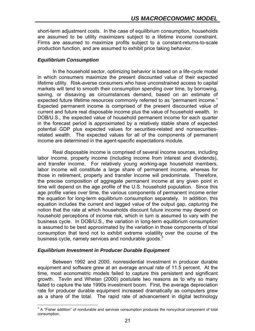
short-term adjustment costs. In the case of equilibrium consumption, households are assumed to be utility maximizers subject to a lifetime income constraint. Firms are assumed to maximize profits subject to a constant-returns-to-scale production function, and are assumed to exhibit price taking behavior. Equilibrium Consumption In the household sector, optimizing behavior is based on a life-cycle model in which consumers maximize the present discounted value of their expected lifetime utility. Risk-averse consumers who have unconstrained access to capital markets will tend to smooth their consumption spending over time, by borrowing, saving, or dissaving as circumstances demand, based on an estimate of expected future lifetime resources commonly referred to as “permanent income.” Expected permanent income is comprised of the present discounted value of current and future real disposable income plus the value of household wealth. In DOB/U.S., the expected value of household permanent income for each quarter in the forecast period is approximated by a relatively stable share of expected potential GDP plus expected values for securities-related and nonsecurities-related wealth. The expected values for all of the components of permanent income are determined in the agent-specific expectations module. Real disposable income is comprised of several income sources, including labor income, property income (including income from interest and dividends), and transfer income. For relatively young working-age household members, labor income will constitute a large share of permanent income, whereas for those in retirement, property and transfer income will predominate. Therefore, the precise composition of aggregate permanent income at any given point in time will depend on the age profile of the U.S. household population. Since this age profile varies over time, the various components of permanent income enter the equation for long-term equilibrium consumption separately. In addition, this equation includes the current and lagged value of the output gap, capturing the notion that the rate at which households discount future income may depend on household perceptions of income risk, which in turn is assumed to vary with the business cycle. In DOB/U.S., the variation in long-term equilibrium consumption is assumed to be best approximated by the variation in those components of total consumption that tend not to exhibit extreme volatility over the course of the business cycle, namely services and nondurable goods.3 Equilibrium Investment in Producer Durable Equipment Between 1992 and 2000, nonresidential investment in producer durable equipment and software grew at an average annual rate of 11.5 percent. At the time, most econometric models failed to capture this persistent and significant growth. Tevlin and Whelan (2000) postulate two reasons as to why so many failed to capture the late 1990s investment boom. First, the average depreciation rate for producer durable equipment increased dramatically as computers grew as a share of the total. The rapid rate of advancement in digital technology 3 A “Fisher addition” of nondurable and services consumption produces the noncyclical component of total consumption.
US MACROECONOMIC MODEL
22
rendered computer and related equipment obsolete in just a few years. Indeed, the depreciation rate for computers and related equipment is more than twice the rate than for other equipment.4 Secondly, investment became more sensitive to the user cost of capital. In order to address these problems, DOB/U.S. estimates investment in computer equipment separately from the remainder of producer durable equipment.5 Figure 3 compares the growth in the two investment components since 1990. Profit-maximizing behavior dictates that the long-term rate of equilibrium investment is the rate of investment that maintains the optimum capital-output ratio. Assuming a standard Cobb-Douglas production function, the optimal capital-output ratio will be proportional to the ratio of the price of output to the rental rate of capital. This relationship holds for both types of producer durable equipment. Given this optimal ratio, desired growth in investment varies with output growth and changes in the rental rate of capital. For each type of equipment, the rental rate of capital is defined as its purchase price, represented by the implicit price deflator, multiplied by the sum of the financial cost of capital and the rate of depreciation. The financial cost of capital, a measure of the cost of borrowing in equity and debt markets, is estimated by giving equal weight to an estimate of the after-tax cost of equity and the yield on Moody’s Baa-rated corporate bonds.6 Different rates of depreciation are used for computer and noncomputer equipment.
Figure 3
Real Producer Durable Equipment Growth
-40
-30
-20
-10
0
10
20
30
40
50
60
1990 1992 1994 1996 1998 2000 2002 2004 2006 2008 2010 2012
Perc
ent c
hang
e ye
ar a
go
ComputerNoncomputer
Note: Shaded areas represent U.S. recessions.Source: Moody’s Economy.com; DOB staff estimates.
Forecast
4 See Fraumeni (1997). 5 The brisk growth of computer equipment as a share of total producer durable equipment may represent in part an error in the data. Chain-weighting tends to overestimate real quantities when prices fall as quickly as those of computers and related equipment. 6 The series that estimates the after-tax cost of borrowing in the equity market is created by Global Insight.
US MACROECONOMIC MODEL
23
Equilibrium Prices, Productivity, Wages, and Hours Worked In equilibrium, the price level is determined by the condition that in competitive markets price equals marginal cost. Long-run productivity growth is determined by a time series model reflecting the belief that its own recent history is the best predictor of future growth. Long-term equilibrium nominal wage growth is determined by the sum of trend productivity growth and the long-term expected rate of inflation. The desired level of man-hours worked is constructed by dividing potential real GDP by trend labor productivity. EXOGENOUS VARIABLES There are many economic variables for which economic theory provides little or no guidance as to either their long-term or short-term behavior. The exogenous variable module estimates future values for over 30 such variables, whose inputs are variables from the shared information set and autoregressive terms. Although a few exogenous variables become inputs to the behavioral equations within the core behavioral module, most are incorporated into identity equations defined to arrive at NIPA concepts. THE CORE BEHAVIORAL MODULE The core behavioral module contains 118 estimating equations, of which 33 are behavioral. The behavioral equations summarize the behavior of representative agents acting with foresight to achieve optimal outcomes in the presence of constraints. In the economy’s real sector, the movement toward equilibrium is hampered, in the short run, by adjustment costs. Through the dynamic adjustment process, agents plan to close the gap between the current level of the variable in question and the desired level. The magnitude of an adjustment made by agents during any given period is based on the size of the gap, past values of the variable, and past and expected values of other variables that may affect agents’ decisions. In the financial sector, agents are assumed to adjust instantaneously when new information becomes available. Therefore, the equations for this sector do not contain any dynamic adjustment terms. The core behavioral module is composed of five sectors: households, firms, government, the financial sector, and the foreign sector. Each is described below. The Household Sector The main decision variables for households are consumption, housing investment, and labor supply. Following Brayton and Tinsley (1996), DOB/U.S. assumes the existence of two groups of consumers. The larger class consists of forward-looking, utility- maximizing consumers whose consumption decisions are constrained by their permanent incomes as defined above. Implicit in the model is the recognition that this group of households is heterogeneous, representing various stages of the lifecycle. The second group is comprised of low-income
US MACROECONOMIC MODEL
24
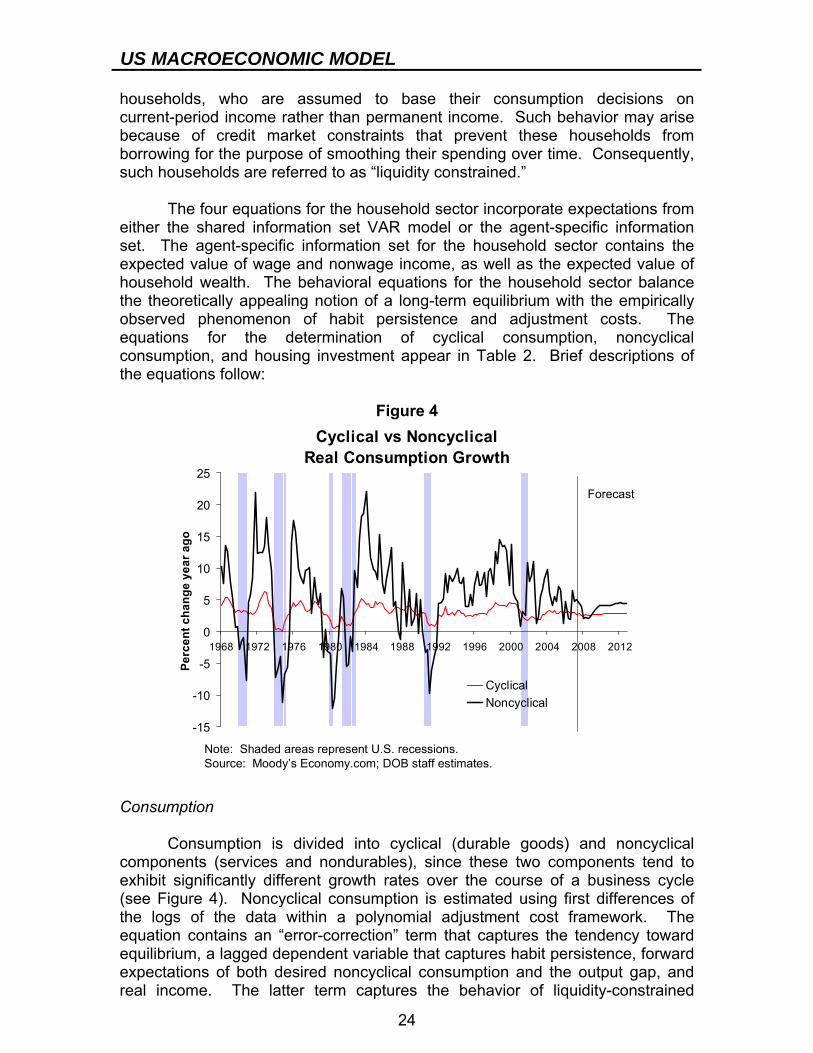
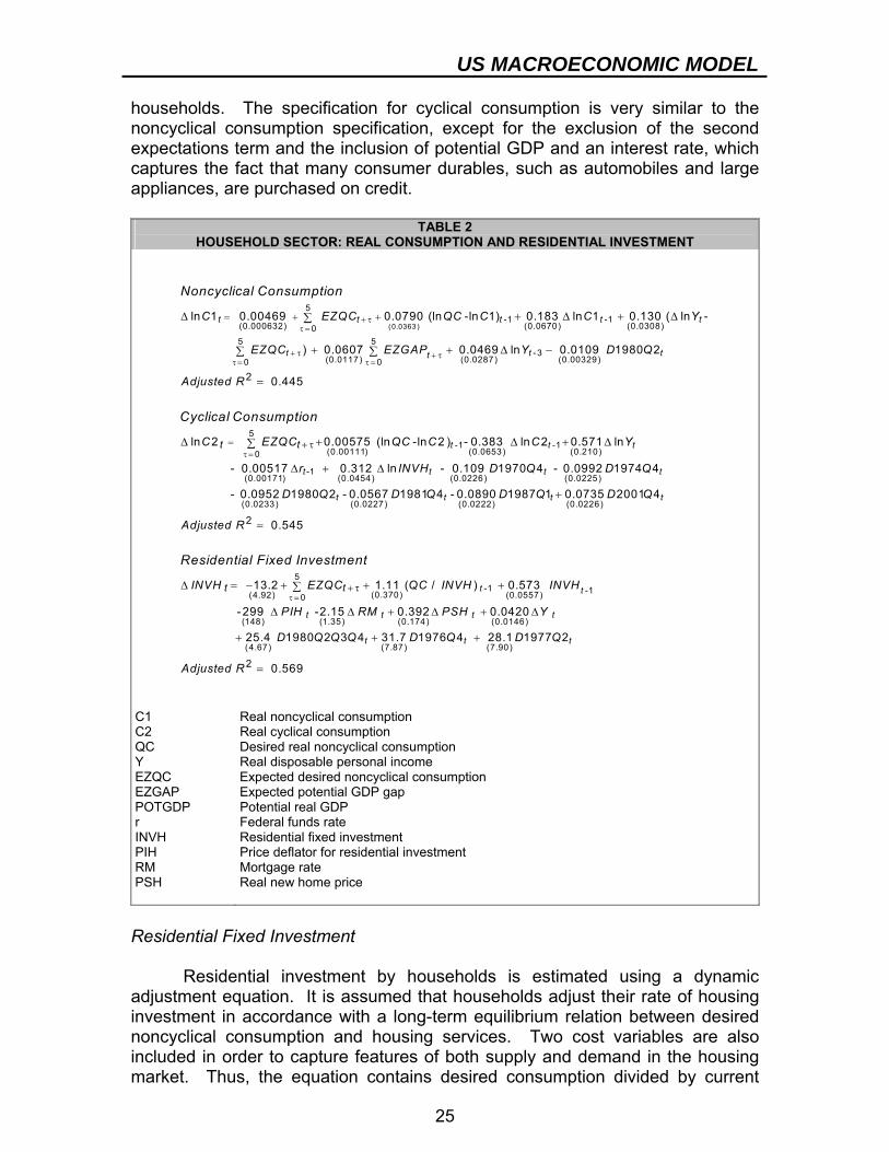
households, who are assumed to base their consumption decisions on current-period income rather than permanent income. Such behavior may arise because of credit market constraints that prevent these households from borrowing for the purpose of smoothing their spending over time. Consequently, such households are referred to as “liquidity constrained.” The four equations for the household sector incorporate expectations from either the shared information set VAR model or the agent-specific information set. The agent-specific information set for the household sector contains the expected value of wage and nonwage income, as well as the expected value of household wealth. The behavioral equations for the household sector balance the theoretically appealing notion of a long-term equilibrium with the empirically observed phenomenon of habit persistence and adjustment costs. The equations for the determination of cyclical consumption, noncyclical consumption, and housing investment appear in Table 2. Brief descriptions of the equations follow:
Figure 4 Cyclical vs Noncyclical
Real Consumption Growth
-15
-10
-5
0
5
10
15
20
25
1968 1972 1976 1980 1984 1988 1992 1996 2000 2004 2008 2012
Perc
ent c
hang
e ye
ar a
go
CyclicalNoncyclical
Note: Shaded areas represent U.S. recessions.Source: Moody’s Economy.com; DOB staff estimates.
Forecast
Consumption Consumption is divided into cyclical (durable goods) and noncyclical components (services and nondurables), since these two components tend to exhibit significantly different growth rates over the course of a business cycle (see Figure 4). Noncyclical consumption is estimated using first differences of the logs of the data within a polynomial adjustment cost framework. The equation contains an “error-correction” term that captures the tendency toward equilibrium, a lagged dependent variable that captures habit persistence, forward expectations of both desired noncyclical consumption and the output gap, and real income. The latter term captures the behavior of liquidity-constrained
US MACROECONOMIC MODEL
25
households. The specification for cyclical consumption is very similar to the noncyclical consumption specification, except for the exclusion of the second expectations term and the inclusion of potential GDP and an interest rate, which captures the fact that many consumer durables, such as automobiles and large appliances, are purchased on credit.
TABLE 2 HOUSEHOLD SECTOR: REAL CONSUMPTION AND RESIDENTIAL INVESTMENT
C1 Real noncyclical consumption C2 Real cyclical consumption QC Desired real noncyclical consumption Y Real disposable personal income EZQC Expected desired noncyclical consumption EZGAP Expected potential GDP gap POTGDP Potential real GDP r Federal funds rate INVH Residential fixed investment PIH Price deflator for residential investment RM Mortgage rate PSH Real new home price Residential Fixed Investment Residential investment by households is estimated using a dynamic adjustment equation. It is assumed that households adjust their rate of housing investment in accordance with a long-term equilibrium relation between desired noncyclical consumption and housing services. Two cost variables are also included in order to capture features of both supply and demand in the housing market. Thus, the equation contains desired consumption divided by current
(0.0363 )
5-1 -1
(0.000632) (0.0670) (0.0308)05 5
-3(0.0117) (0.0287)0 0
ln 1 0.00469 0.0790 (ln -ln 1) 0.183 ln 1 0.130 ( ln -
) 0.0607 0.0469 ln 0.010
t t t t t
t tt
C EZQC QC C C Y
EZQC EZGAP Y
Noncyclical Consumption
+ ττ =
+ τ + ττ= τ =
= + +Δ + Δ + Δ∑
+ + Δ −∑ ∑(0.00329)
5-1 -1
(0.00111) (0.0653) (0.210)0
-1(0.00171) (0.0454) (0.02
2
9 1980 2
0.445
ln 2 0.00575 (ln -ln 2 ) - 0.383 ln 2 0.571 ln
- 0.00517 0.312 ln - 0.109
t
t t t
t t
t t
D Q
Adjusted R
C EZQC QC C C Y
r INVH
Cyclical Consumption
τ == + τ
=
Δ + Δ + Δ∑
Δ + Δ26) (0.0225)
(0.0233) (0.0227) (0.0222) (0.0226)
5
(4.92) 0
2
1970 4 - 0.0992 1974 4
- 0.0952 1980 2 - 0.0567 1981 4 - 0.0890 1987 1 0.0735 2001 4
0.545
13.2
t t
t t t t
t t
D Q D Q
D Q D Q D Q D Q
Adjusted R
INVH EZQC
Residential Fixed Investment
τ =+ τ
+
=
Δ = − + +∑ -1 -1(0.370) (0.0557)
(148) (1.35) (0.174) (0.0146)
(4.67) (7.87) (7.90)
2
1.11 ( / ) 0.573
-299 -2.15 0.392 0.0420
25.4 1980 2 3 4 31.7 1976 4 28.1 1977 2
0.569
t t
t t t t
t t t
QC INVH INVH
PIH RM PSH Y
D Q Q Q D Q D Q
Adjusted R
+
Δ Δ + Δ + Δ
+ + +
=
US MACROECONOMIC MODEL
26
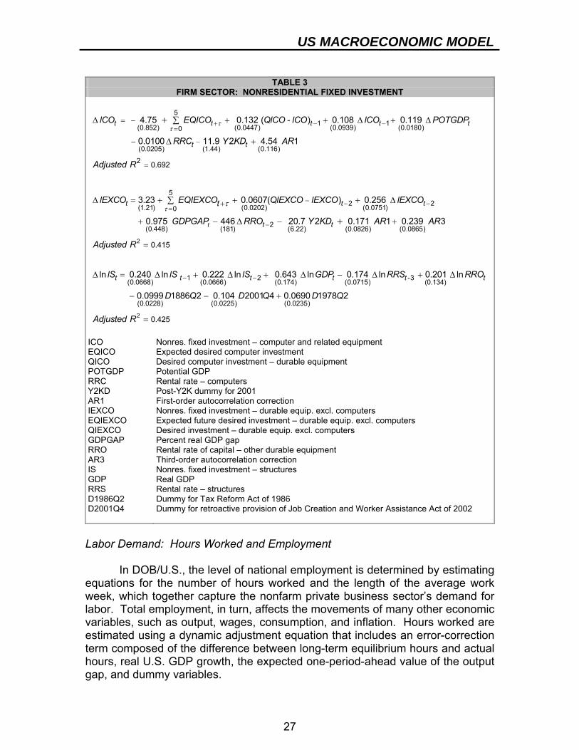
housing investment, a lagged endogenous variable to capture habit persistence, forward-looking expectations of desired consumption, the mortgage rate, the price deflator for residential investment, and the real average price of one-family homes sold. Labor Supply Households must make decisions about how much labor they supply to the labor market. In DOB/U.S., the behavioral equation which determines the first difference of the labor force participation rate includes its own lags; real GDP lagged three quarters; a dummy variable capturing the influx of women into the labor market in the 1960s, 1970s, and 1980s; and dummy variables capturing the extraordinary increases in hiring census workers in the first quarters of 1990 and 2000 for the decennial censuses. The labor supply is then determined by multiplying the labor force participation rate by an estimate of the working-age population (ages 16 through 64). The Firm Sector DOB/U.S. incorporates the assumption that firms set their prices and levels of factor inputs used in production to maximize profits. This sector determines the levels of the two components of nonresidential fixed investment, private nonresidential structures, labor demand, real wages, and output prices. Like the behavioral equations describing the household sector, several of the firm sector equations incorporate both error-correction terms to capture the impact of long-term equilibrium relationships and dynamic adjustment terms to capture firm-level adjustment costs. The behavioral equations for investment in computer-related producer durable equipment, all other producer durable equipment, and nonresidential structures appear in Table 3. Nonresidential Investment DOB/U.S. estimates three categories of nonresidential investment: investment in computer-related producer durable equipment and software, investment in all other equipment, and investment in nonresidential structures. The estimating equations for investment in computer and related equipment and all other equipment are virtually identical. Both equations contain an error-correction term, defined as a lag difference between equilibrium and current investment, an autoregressive term, forward expectations of equilibrium investment, and the appropriate rental rate of capital, as defined above. Longer lags yield a superior fit in the equation for noncomputer equipment due to its relatively low depreciation rate. In addition, the computer equipment equation contains the first difference in potential GDP growth and a dummy variable to capture the large decline in investment during the second and third quarters of 2001. The equation for noncomputer equipment contains the current period value for the output gap. Investment in nonresidential structures is determined by its own rental rate, real U.S. GDP growth, as well as its own past values and dummy variables.
US MACROECONOMIC MODEL
27
TABLE 3
FIRM SECTOR: NONRESIDENTIAL FIXED INVESTMENT
51 1(0.852) (0.0447) (0.0939) (0.0180)0
(0.0205) (1.44) (0.116)
2
(1.21)
0.692
4.75 0.132 ( - ) 0.108 0.119
0.0100 11.9 2 4.54 1
3.23
t t t t t
t t
t t
lCO EQICO QlCO lCO lCO POTGDP
RRC Y KD AR
Adjusted R
lEXCO EQIEXCO
ττ
ττ
+ − −=
−
= −
=
−
+
Δ + + Δ + Δ∑
Δ +
Δ = + +
+
2
52 2(0.0202) (0.0751)0
2(0.448) (181) (6.22) (0.0826) (0.0865)
1(0.0668) (0.066
0.415
0.0607( ) 0.256
0.975 446 20.7 2 0.171 1 0.239 3
ln 0.240 ln 0.222
t
t t
t t
t t
QlEXCO lEXCO lEXCO
GDPGAP RRO Y KD AR AR
Adjusted R
lS lS
− −=
−
−
− + Δ∑
+ − Δ − +
=
Δ = Δ +
+
2
2 -36) (0.174) (0.0715) (0.134)
(0.0228) (0.0225) (0.0235)
0.425
ln 0.643 ln 0.174 ln 0.201 ln
0.0999 1886 2 0.104 2001 4 0.0690 1978 2
t t t tlS GDP RRS RRO
D Q D Q D Q
Adjusted R
−Δ + Δ − Δ + Δ
− − +
= ICO Nonres. fixed investment – computer and related equipment EQICO Expected desired computer investment QICO Desired computer investment – durable equipment POTGDP Potential GDP RRC Rental rate – computers Y2KD Post-Y2K dummy for 2001 AR1 First-order autocorrelation correction IEXCO Nonres. fixed investment – durable equip. excl. computers EQIEXCO Expected future desired investment – durable equip. excl. computers QIEXCO Desired investment – durable equip. excl. computers GDPGAP Percent real GDP gap RRO Rental rate of capital – other durable equipment AR3 Third-order autocorrelation correction IS Nonres. fixed investment – structures GDP Real GDP RRS Rental rate – structures D1986Q2 Dummy for Tax Reform Act of 1986 D2001Q4 Dummy for retroactive provision of Job Creation and Worker Assistance Act of 2002 Labor Demand: Hours Worked and Employment In DOB/U.S., the level of national employment is determined by estimating equations for the number of hours worked and the length of the average work week, which together capture the nonfarm private business sector’s demand for labor. Total employment, in turn, affects the movements of many other economic variables, such as output, wages, consumption, and inflation. Hours worked are estimated using a dynamic adjustment equation that includes an error-correction term composed of the difference between long-term equilibrium hours and actual hours, real U.S. GDP growth, the expected one-period-ahead value of the output gap, and dummy variables.
US MACROECONOMIC MODEL
28
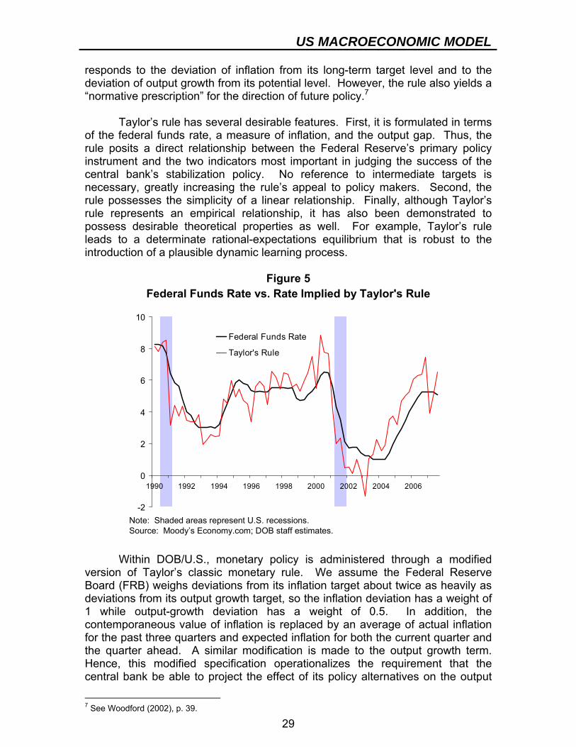
The estimating equation for the average length of the workweek in the private nonfarm business sector also contains an error-correction term and the expected one-period-ahead value of the output gap. In addition, the model includes growth in real private nonfarm business GDP and dummy variables. The level of total private nonfarm employment is determined by dividing hours worked by the average length of the workweek multiplied by the number of weeks in a year. The Wage Rate The average hourly wage rate is defined as total private employee compensation (cash wages and salaries plus additional costs such as medical insurance premiums and employer contributions for social insurance) divided by hours worked. The long-run equilibrium growth in the wage rate is assumed to depend on trend productivity growth and the inflation rate, where inflation is measured by the private nonfarm chain-weighted GDP deflator and productivity is private nonfarm output divided by hours worked adjusted to remove the effects of the business cycle. Thus, the equilibrium wage rate at time t is its value at time t-1 plus the sum of the growth rates for productivity and inflation. The actual quarterly wage rate is modeled in an error correction framework but contains additional lags capturing the presence of “wage-stickiness.” The model also includes the expected one-period-ahead value of the output gap to capture the impact of forward-looking behavior on the speed of adjustment toward equilibrium. Output Prices The price level is represented by the private nonfarm chain-weighted GDP deflator. Its growth is modeled within a dynamic adjustment framework in which the price level adjusts gradually from its current level to its long-term equilibrium value. The model also includes the expected one- and two-period-ahead values of the output gap, again to capture the impact of forward-looking behavior on the speed of adjustment toward equilibrium. In addition, the model contains the petroleum products component of the Producer Price Index (PPI) to capture the impact of wholesale energy prices, as well as dummy variables to capture the impact of the 1970s oil shocks above and beyond what is captured by the PPI. The Government Sector Monetary policy affects economic and financial decisions made by agents in the economy. The objective of monetary policy is to stabilize the economy’s performance — as reflected in the behavior of inflation, output, and employment — by balancing the twin goals of sustainable growth and price stability. This is accomplished by raising or lowering short-term interest rates through changes in the central bank’s target federal funds rate in a manner that is consistent with price stability and sustainable growth. Taylor’s rule approximates the way the Federal Reserve has historically conducted monetary policy, particularly when the classic rule is augmented by expectations over future inflation and output (see Figure 5). Taylor’s rule is a federal funds rate reaction function that
US MACROECONOMIC MODEL
29
responds to the deviation of inflation from its long-term target level and to the deviation of output growth from its potential level. However, the rule also yields a “normative prescription” for the direction of future policy.7 Taylor’s rule has several desirable features. First, it is formulated in terms of the federal funds rate, a measure of inflation, and the output gap. Thus, the rule posits a direct relationship between the Federal Reserve’s primary policy instrument and the two indicators most important in judging the success of the central bank’s stabilization policy. No reference to intermediate targets is necessary, greatly increasing the rule’s appeal to policy makers. Second, the rule possesses the simplicity of a linear relationship. Finally, although Taylor’s rule represents an empirical relationship, it has also been demonstrated to possess desirable theoretical properties as well. For example, Taylor’s rule leads to a determinate rational-expectations equilibrium that is robust to the introduction of a plausible dynamic learning process.
Figure 5
-2
0
2
4
6
8
10
1990 1992 1994 1996 1998 2000 2002 2004 2006
Federal Funds Rate
Taylor's Rule
Note: Shaded areas represent U.S. recessions.Source: Moody’s Economy.com; DOB staff estimates.
Federal Funds Rate vs. Rate Implied by Taylor's Rule
Within DOB/U.S., monetary policy is administered through a modified version of Taylor’s classic monetary rule. We assume the Federal Reserve Board (FRB) weighs deviations from its inflation target about twice as heavily as deviations from its output growth target, so the inflation deviation has a weight of 1 while output-growth deviation has a weight of 0.5. In addition, the contemporaneous value of inflation is replaced by an average of actual inflation for the past three quarters and expected inflation for both the current quarter and the quarter ahead. A similar modification is made to the output growth term. Hence, this modified specification operationalizes the requirement that the central bank be able to project the effect of its policy alternatives on the output
7 See Woodford (2002), p. 39.
US MACROECONOMIC MODEL
30
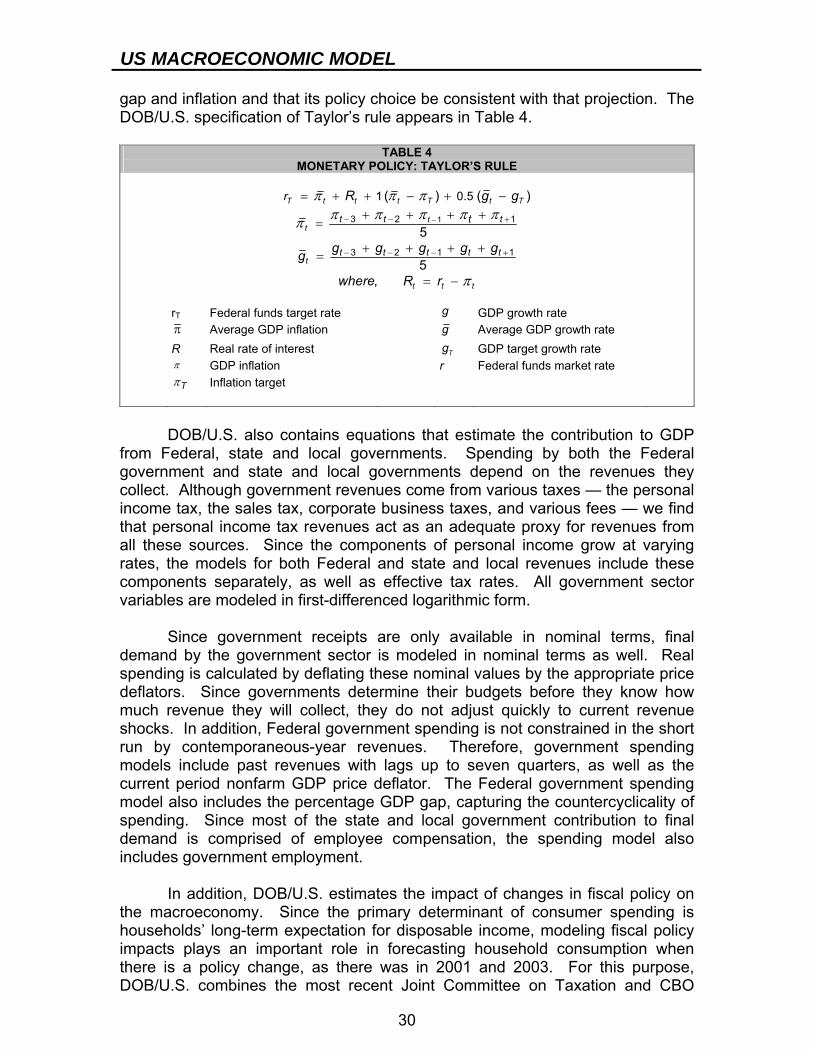
gap and inflation and that its policy choice be consistent with that projection. The DOB/U.S. specification of Taylor’s rule appears in Table 4.
TABLE 4 MONETARY POLICY: TAYLOR’S RULE
13 2 1
3 2 1 1
1 0.5( ) ( )
5
5,
T t t t T t T
tt
t
t t t
t t t
t t t t t
t
r R g g
g g g g gg
where R r
π π ππ π π π ππ
π
−− − +
− − − +
= + + − + −+ + + +
=
+ + + +=
= − rT Federal funds target rate g GDP growth rate π Average GDP inflation g Average GDP growth rate R Real rate of interest Tg GDP target growth rate π GDP inflation r Federal funds market rate Tπ Inflation target DOB/U.S. also contains equations that estimate the contribution to GDP from Federal, state and local governments. Spending by both the Federal government and state and local governments depend on the revenues they collect. Although government revenues come from various taxes — the personal income tax, the sales tax, corporate business taxes, and various fees — we find that personal income tax revenues act as an adequate proxy for revenues from all these sources. Since the components of personal income grow at varying rates, the models for both Federal and state and local revenues include these components separately, as well as effective tax rates. All government sector variables are modeled in first-differenced logarithmic form. Since government receipts are only available in nominal terms, final demand by the government sector is modeled in nominal terms as well. Real spending is calculated by deflating these nominal values by the appropriate price deflators. Since governments determine their budgets before they know how much revenue they will collect, they do not adjust quickly to current revenue shocks. In addition, Federal government spending is not constrained in the short run by contemporaneous-year revenues. Therefore, government spending models include past revenues with lags up to seven quarters, as well as the current period nonfarm GDP price deflator. The Federal government spending model also includes the percentage GDP gap, capturing the countercyclicality of spending. Since most of the state and local government contribution to final demand is comprised of employee compensation, the spending model also includes government employment. In addition, DOB/U.S. estimates the impact of changes in fiscal policy on the macroeconomy. Since the primary determinant of consumer spending is households’ long-term expectation for disposable income, modeling fiscal policy impacts plays an important role in forecasting household consumption when there is a policy change, as there was in 2001 and 2003. For this purpose, DOB/U.S. combines the most recent Joint Committee on Taxation and CBO
US MACROECONOMIC MODEL
31
estimates where available with results from the Current Expenditure Survey data, disaggregated by income level, to estimate how much of the change in disposable income will affect consumption. The Financial Sector The financial sector of DOB/U.S. is subdivided into two blocks of equations: one determining equity prices and the other determining interest rates. Many analysts believe that short-run changes in stock market prices follow a random walk and therefore it is impossible to forecast the day-to-day movements of individual stocks with any accuracy. However, long-run movements in price indices of large groups of stocks appear to move systematically with other economic variables. Much of the variation in the growth of the Standard & Poor’s 500 price index can be explained by the contemporaneous and expected growth of pre-tax corporate profits after normalizing by the interest rate on Baa corporate bonds. A lead term is added to capture the influence of profit expectations on investors’ decisions to buy and sell equities, and, consequently, on stock prices. In addition to the federal funds rate, which is modeled based on Taylor's Rule, DOB/U.S. contains models for six interest rates: the three-month, one-year, five-year, and ten-year U.S. Treasury securities rates, as well as the Baa corporate bond rate and the 30-year conventional mortgage rate. These equations are specified within an error-correction model framework based on the expectations theory of the term structure of interest rates, which posits that the yield on the long-term bond equals the expected yield on a series of short-term bonds over the life of the long-term bond, plus term and risk premiums. The theory implies that the rate on one-year government bonds can be used to explain the rate on five-year bonds, which, in turn, is used to explain the rate on bonds of longer maturities. Although the term and risk premiums are not explicitly captured in the estimated model, their impacts are embodied in the estimated coefficients. A real GDP gap term is added to most of the equations to capture the impact of expected (future) inflationary pressures on current yield curve. The Foreign Sector Real U.S. exports are determined by the level of foreign economic activity, as measured by an estimate of the growth rate of global GDP and U.S. export prices relative to foreign prices. Real imports are divided into non-oil and oil goods and services. Non-oil imports are a function of real domestic demand and the ratio of import prices to domestic prices. Oil imports are a function of real domestic demand, as well as oil prices relative to domestic prices. Both imports and exports equations contain additional dummy variables to capture one-time shocks, such as the September 11 terrorist attacks and the oil shocks of the 1970s.
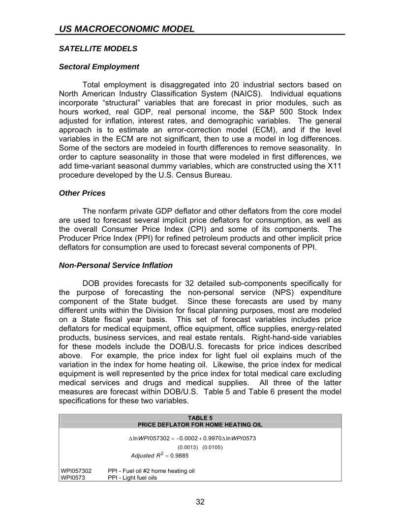
US MACROECONOMIC MODEL
32
SATELLITE MODELS Sectoral Employment Total employment is disaggregated into 20 industrial sectors based on North American Industry Classification System (NAICS). Individual equations incorporate “structural” variables that are forecast in prior modules, such as hours worked, real GDP, real personal income, the S&P 500 Stock Index adjusted for inflation, interest rates, and demographic variables. The general approach is to estimate an error-correction model (ECM), and if the level variables in the ECM are not significant, then to use a model in log differences. Some of the sectors are modeled in fourth differences to remove seasonality. In order to capture seasonality in those that were modeled in first differences, we add time-variant seasonal dummy variables, which are constructed using the X11 procedure developed by the U.S. Census Bureau. Other Prices The nonfarm private GDP deflator and other deflators from the core model are used to forecast several implicit price deflators for consumption, as well as the overall Consumer Price Index (CPI) and some of its components. The Producer Price Index (PPI) for refined petroleum products and other implicit price deflators for consumption are used to forecast several components of PPI. Non-Personal Service Inflation DOB provides forecasts for 32 detailed sub-components specifically for the purpose of forecasting the non-personal service (NPS) expenditure component of the State budget. Since these forecasts are used by many different units within the Division for fiscal planning purposes, most are modeled on a State fiscal year basis. This set of forecast variables includes price deflators for medical equipment, office equipment, office supplies, energy-related products, business services, and real estate rentals. Right-hand-side variables for these models include the DOB/U.S. forecasts for price indices described above. For example, the price index for light fuel oil explains much of the variation in the index for home heating oil. Likewise, the price index for medical equipment is well represented by the price index for total medical care excluding medical services and drugs and medical supplies. All three of the latter measures are forecast within DOB/U.S. Table 5 and Table 6 present the model specifications for these two variables.
TABLE 5 PRICE DEFLATOR FOR HOME HEATING OIL
Δ = − + Δ
=2(0.0013) (0.0105)
ln 057302 0.0002 0.9970 ln 0573
0.9885
WPI WPI
Adjusted R WPI057302 PPI - Fuel oil #2 home heating oil WPI0573 PPI - Light fuel oils
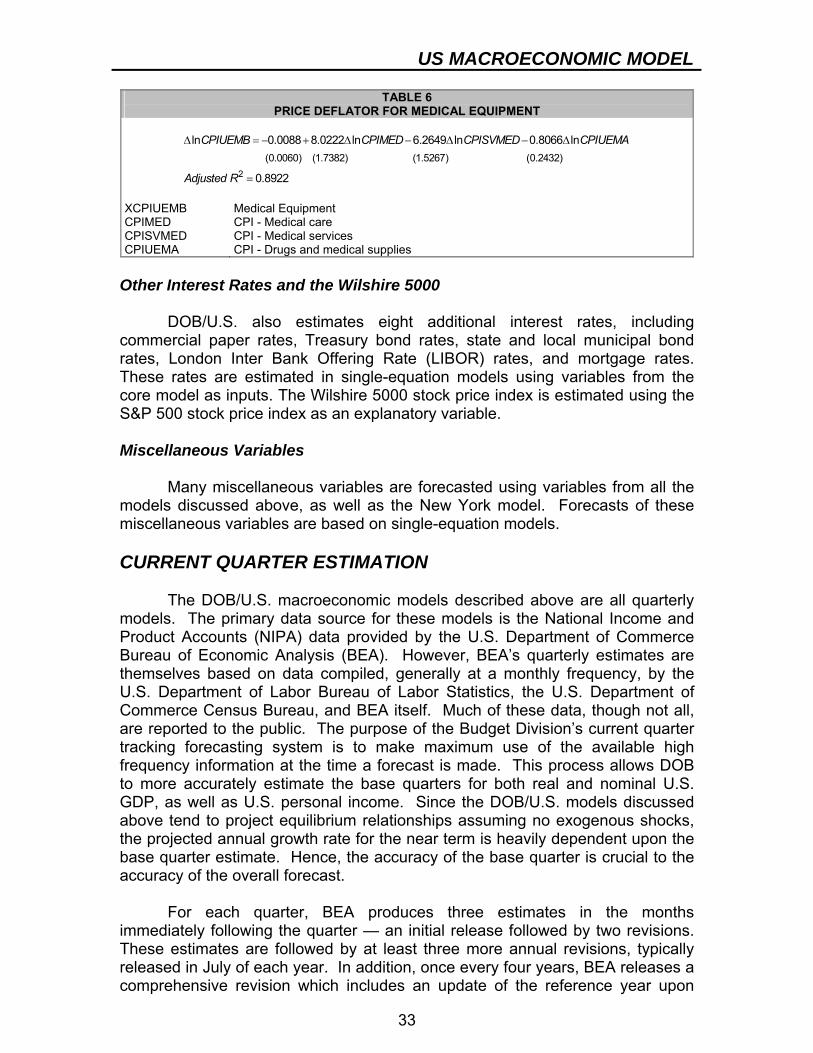
US MACROECONOMIC MODEL
33
TABLE 6 PRICE DEFLATOR FOR MEDICAL EQUIPMENT
Δ = − + Δ − Δ − Δ
=2
(0.0060) (1.7382) (1.5267) (0.2432)
ln 0.0088 8.0222 ln 6.2649 ln 0.8066 ln
0.8922
CPIUEMB CPIMED CPISVMED CPIUEMA
Adjusted R XCPIUEMB Medical Equipment CPIMED CPI - Medical care CPISVMED CPI - Medical services CPIUEMA CPI - Drugs and medical supplies
Other Interest Rates and the Wilshire 5000 DOB/U.S. also estimates eight additional interest rates, including commercial paper rates, Treasury bond rates, state and local municipal bond rates, London Inter Bank Offering Rate (LIBOR) rates, and mortgage rates. These rates are estimated in single-equation models using variables from the core model as inputs. The Wilshire 5000 stock price index is estimated using the S&P 500 stock price index as an explanatory variable. Miscellaneous Variables Many miscellaneous variables are forecasted using variables from all the models discussed above, as well as the New York model. Forecasts of these miscellaneous variables are based on single-equation models. CURRENT QUARTER ESTIMATION The DOB/U.S. macroeconomic models described above are all quarterly models. The primary data source for these models is the National Income and Product Accounts (NIPA) data provided by the U.S. Department of Commerce Bureau of Economic Analysis (BEA). However, BEA’s quarterly estimates are themselves based on data compiled, generally at a monthly frequency, by the U.S. Department of Labor Bureau of Labor Statistics, the U.S. Department of Commerce Census Bureau, and BEA itself. Much of these data, though not all, are reported to the public. The purpose of the Budget Division’s current quarter tracking forecasting system is to make maximum use of the available high frequency information at the time a forecast is made. This process allows DOB to more accurately estimate the base quarters for both real and nominal U.S. GDP, as well as U.S. personal income. Since the DOB/U.S. models discussed above tend to project equilibrium relationships assuming no exogenous shocks, the projected annual growth rate for the near term is heavily dependent upon the base quarter estimate. Hence, the accuracy of the base quarter is crucial to the accuracy of the overall forecast. For each quarter, BEA produces three estimates in the months immediately following the quarter — an initial release followed by two revisions. These estimates are followed by at least three more annual revisions, typically released in July of each year. In addition, once every four years, BEA releases a comprehensive revision which includes an update of the reference year upon
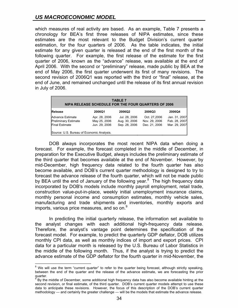
US MACROECONOMIC MODEL
34
which measures of real activity are based. As an example, Table 7 presents a chronology for BEA’s first three releases of NIPA estimates, since these estimates are the most relevant to the Budget Division’s current quarter estimation, for the four quarters of 2006. As the table indicates, the initial estimate for any given quarter is released at the end of the first month of the following quarter. For example, the first release of the estimate for the first quarter of 2006, known as the “advance” release, was available at the end of April 2006. With the second or “preliminary” release, made public by BEA at the end of May 2006, the first quarter underwent its first of many revisions. The second revision of 2006Q1 was reported with the third or “final” release, at the end of June, and remained unchanged until the release of its first annual revision in July of 2006.
TABLE 7 NIPA RELEASE SCHEDULE FOR THE FOUR QUARTERS OF 2006
Release 2006Q1 2006Q2 2006Q3 2006Q4
Advance Estimate Apr. 28, 2006 Jul. 28, 2006 Oct. 27,2006 Jan. 31, 2007Preliminary Estimate May 25, 2006 Aug. 30, 2006 Nov. 29, 2006 Feb. 28, 2007Final Estimate Jun. 29, 2006 Sep. 28, 2006 Dec. 21, 2006 Mar. 29, 2007 Source: U.S. Bureau of Economic Analysis.
DOB always incorporates the most recent NIPA data when doing a forecast. For example, the forecast completed in the middle of December, in preparation for the Executive Budget, always includes the preliminary estimate of the third quarter that becomes available at the end of November. However, by mid-December, high frequency data related to the fourth quarter has also become available, and DOB’s current quarter methodology is designed to try to forecast the advance release of the fourth quarter, which will not be made public by BEA until the end of January of the following year.8 The high frequency data incorporated by DOB's models include monthly payroll employment, retail trade, construction value-put-in-place, weekly initial unemployment insurance claims, monthly personal income and consumption estimates, monthly vehicle sales, manufacturing and trade shipments and inventories, monthly exports and imports, various price measures, and so on.9 In predicting the initial quarterly release, the information set available to the analyst changes with each additional high-frequency data release. Therefore, the analyst’s vantage point determines the specification of the forecast model. For example, to predict the quarterly GDP deflator, DOB utilizes monthly CPI data, as well as monthly indices of import and export prices. CPI data for a particular month is released by the U.S. Bureau of Labor Statistics in the middle of the following month. Thus, if the analyst is trying to predict the advance estimate of the GDP deflator for the fourth quarter in mid-November, the 8 We will use the term “current quarter” to refer to the quarter being forecast, although strictly speaking, between the end of the quarter and the release of the advance estimate, we are forecasting the prior quarter. 9 By the middle of December, some additional high frequency data has also become available hinting at the second revision, or final estimate, of the third quarter. DOB’s current quarter models attempt to use these data to anticipate these revisions. However, the focus of this description of the DOB’s current quarter methodology — and certainly the greater challenge — will be the models that estimate the advance release.
US MACROECONOMIC MODEL
35
relevant information set contains only one month of CPI, import price, and export price data for the quarter, i.e., for October, and the model specification can only include that one month. However, if a forecast is being done in mid-December, the information set contains two months of data, October and November. Thus, a second specification is required to be able to incorporate that information as well. Finally, by mid-January, all three months of CPI data for the quarter are available, suggesting yet a third specification. Finally, if a forecast is done between the release of the CPI and the trade price data, yet another specification might be necessary. On average, forecast models are run from six different vantage points leading up to the NIPA advance release, although that number may vary depending on the demands of the Division’s U.S. macromodel forecasting schedule. In addition to the GDP price deflator, DOB has developed forecasting models for the following nominal and real GDP components: durable, nondurable, and services consumption; fixed residential investment; business sector fixed investment in computer and computer-related durable equipment and software, noncomputer equipment, and structures; the change in inventories; federal government defense consumption and investment and nondefense consumption and investment spending; state and local government consumption and investment spending; oil and non-oil imports; and exports. Real U.S. GDP is calculated two ways: first, by dividing the sum of the nominal components by the price deflator, and second, by “Fisher adding” the real components. If the two methods produce different outcomes, adjustments are made before incorporating the results into DOB/U.S. Current quarter models have also been developed for the following components of national personal income: wages and salary disbursements, transfer payments to persons, personal contributions for social insurance, other labor income, rental income of persons with the capital consumption adjustment (CCA), personal dividend income, personal interest income, and proprietors’ income with the inventory valuation adjustment (IVA) and CCA. Examples of models for one real GDP component, two components of personal income, as well as additional detail pertaining to the GDP deflator appear below. In the interest of space, models for only three vantages are presented. GDP DEFLATOR As alluded to above, the current quarter GDP deflator is a function of the monthly CPI and the price deflators for imports and exports. The left-hand side variable is quarterly growth at seasonally adjusted annualized rates (SAAR). The right-hand side concepts are also annualized quarterly growth rates, though their precise specification varies with the data available, as well as the results of empirical testing. Table 8 presents model specifications for three vantages. The first vantage includes the annualized growth rate of the first month of the current quarter over the first month of the previous quarter for CPI and for import prices, while the price deflator for exports enters as a “momentum term.” The latter term captures the mathematical fact that greater the growth in the first month of the
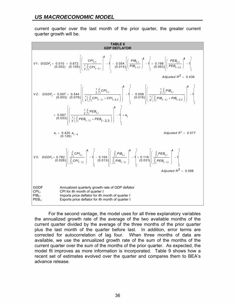
US MACROECONOMIC MODEL
36
current quarter over the last month of the prior quarter, the greater current quarter growth will be.
TABLE 8 GDP DEFLATOR
GGDF Annualized quarterly growth rate of GDP deflator CPIt,i CPI for ith month of quarter t PIBt,i Imports price deflator for ith month of quarter t PEBt,i Exports price deflator for ith month of quarter t For the second vantage, the model uses for all three explanatory variables the annualized growth rate of the average of the two available months of the current quarter divided by the average of the three months of the prior quarter plus the last month of the quarter before last. In addition, error terms are corrected for autocorrelation of lag four. When three months of data are available, we use the annualized growth rate of the sum of the months of the current quarter over the sum of the months of the prior quarter. As expected, the model fit improves as more information is incorporated. Table 9 shows how a recent set of estimates evolved over the quarter and compares them to BEA’s advance release.
3
1
,1 ,1 ,11
-1,1 -1,31,3
4 4 41: 0.010 0.672 1 0.054 1 0.198 1
(0.002) (0.109) (0.014) (0.063)i
t t tt
t tt i
CPI PIB PEBV GGDF
PIB PEBCPI= −∑
⎡ ⎤⎛ ⎞ ⎡ ⎤ ⎡ ⎤⎢ ⎥ ⎛ ⎞ ⎛ ⎞⎜ ⎟ ⎢ ⎥ ⎢ ⎥⎢ ⎥ ⎜ ⎟ ⎜ ⎟= + − − − + −⎜ ⎟ ⎢ ⎥ ⎢ ⎥⎢ ⎥ ⎜ ⎟ ⎜ ⎟⎜ ⎟ ⎢ ⎥ ⎢ ⎥⎝ ⎠ ⎝ ⎠⎢ ⎥ ⎣ ⎦ ⎣ ⎦⎝ ⎠⎣ ⎦
2
13
1
1,2
11, -2,34
2 0.436
2 : 0.007 0.544(0.003) (0.079)
i
i
t it
t i t
Adjusted R
CPIV GGDF
CPI CPI
=
= −
∑
∑
=
= ++
2
13
1
2
13
1
1,2
11, -2,34
1,2
11,4
4 4
1 0.058 1(0.016)
0.067(0.033)
- 2,3
i
i
i
i
t i
t i t
t i
t i
PIB
PIB PIB
PEB
PEB PEBt
=
=
=
=
−
−
∑
∑
∑
∑
⎡ ⎤ ⎡ ⎤⎛ ⎞ ⎛ ⎞⎢ ⎥ ⎢ ⎥⎜ ⎟ ⎜ ⎟⎢ ⎥ ⎢ ⎥⎜ ⎟ ⎜ ⎟− − −⎢ ⎥ ⎢ ⎥⎛ ⎞ ⎛ ⎞⎜ ⎟ ⎜ ⎟+⎢ ⎥ ⎢ ⎥⎜ ⎟ ⎜ ⎟⎜ ⎟ ⎜ ⎟⎝ ⎠ ⎝ ⎠⎝ ⎠ ⎝ ⎠⎢ ⎥ ⎢ ⎥⎣ ⎦ ⎣ ⎦
⎛⎜⎜+
⎛ ⎞+⎜ ⎟⎝ ⎠⎝
24
4
1
0.420 0.577(0.126)
t
t
t
e
e e Adjusted R−
⎡ ⎤⎞⎢ ⎥⎟⎢ ⎥⎟ − +⎢ ⎥⎜ ⎟⎢ ⎥⎜ ⎟⎠⎢ ⎥⎣ ⎦
= =
3
13
1
, ,
1,
4
3: 0.782 1 0.104(0.026) (0.013)
i i
i
t i t it
t i
CPI PIBV GGDF
CPI=
= −
∑
∑
⎡ ⎤⎛ ⎞⎢ ⎥⎜ ⎟⎢ ⎥= − −⎜ ⎟⎢ ⎥⎜ ⎟⎢ ⎥⎝ ⎠⎢ ⎥⎣ ⎦
3 3
1 13 3
1 1
,
1, 1,
4 4
1 0.116 1(0.031)
i
i i
t i
t i t i
PEB
PIB PEB= =
= =− −
∑ ∑
∑ ∑
⎡ ⎤ ⎡ ⎤⎛ ⎞ ⎛ ⎞⎢ ⎥ ⎢ ⎥⎜ ⎟ ⎜ ⎟⎢ ⎥ ⎢ ⎥− + −⎜ ⎟ ⎜ ⎟⎢ ⎥ ⎢ ⎥⎜ ⎟ ⎜ ⎟⎢ ⎥ ⎢ ⎥⎝ ⎠ ⎝ ⎠⎢ ⎥ ⎢ ⎥⎣ ⎦ ⎣ ⎦
2 0.598Adjusted R =
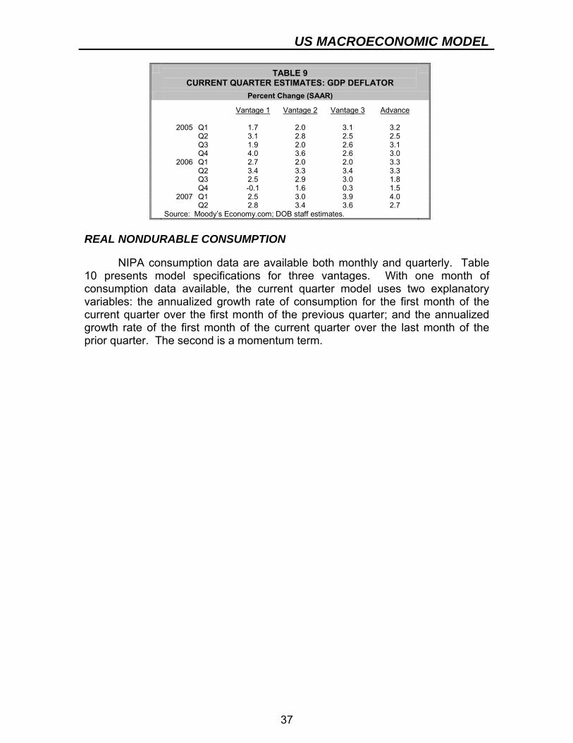
US MACROECONOMIC MODEL
37
TABLE 9 CURRENT QUARTER ESTIMATES: GDP DEFLATOR
Percent Change (SAAR)
Vantage 1 Vantage 2 Vantage 3 Advance 2005 Q1 1.7 2.0 3.1 3.2 Q2 3.1 2.8 2.5 2.5 Q3 1.9 2.0 2.6 3.1 Q4 4.0 3.6 2.6 3.0 2006 Q1 2.7 2.0 2.0 3.3 Q2 3.4 3.3 3.4 3.3 Q3 2.5 2.9 3.0 1.8 Q4 -0.1 1.6 0.3 1.5 2007 Q1 2.5 3.0 3.9 4.0 Q2 2.8 3.4 3.6 2.7 Source: Moody’s Economy.com; DOB staff estimates.
REAL NONDURABLE CONSUMPTION NIPA consumption data are available both monthly and quarterly. Table 10 presents model specifications for three vantages. With one month of consumption data available, the current quarter model uses two explanatory variables: the annualized growth rate of consumption for the first month of the current quarter over the first month of the previous quarter; and the annualized growth rate of the first month of the current quarter over the last month of the prior quarter. The second is a momentum term.
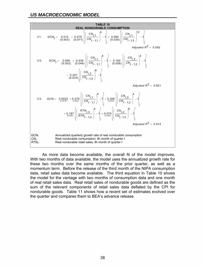
US MACROECONOMIC MODEL
38
TABLE 10 REAL NONDURABLE CONSUMPTION
GCNt Annualized quarterly growth rate of real nondurable consumption CNt,i Real nondurable consumption; ith month of quarter t RTNt,i Real nondurable retail sales; ith month of quarter t As more data become available, the overall fit of the model improves. With two months of data available, the model uses the annualized growth rate for these two months over the same months of the prior quarter, as well as a momentum term. Before the release of the third month of the NIPA consumption data, retail sales data become available. The third equation in Table 10 shows the model for the vantage with two months of consumption data and one month of real retail sales data. Real retail sales of nondurable goods are defined as the sum of the relevant components of retail sales data deflated by the CPI for nondurable goods. Table 11 shows how a recent set of estimates evolved over the quarter and compares them to BEA’s advance release.
4 12,1 ,11: 0.014 0.479 1 0.084 1
(0.003) (0.071) (0.026)1,1 - 1,3
CN CNt tV GCNt CN CNt t
⎡ ⎤ ⎡ ⎤⎛ ⎞ ⎛ ⎞⎢ ⎥ ⎢ ⎥⎜ ⎟ ⎜ ⎟= + − + −⎢ ⎥ ⎢ ⎥⎜ ⎟ ⎜ ⎟⎢ ⎥ ⎢ ⎥−⎝ ⎠ ⎝ ⎠⎢ ⎥ ⎢ ⎥⎣ ⎦ ⎣ ⎦
2 0.592
4 4,1 ,22 : 0.006 0.439 1 0.180 1
(0.002) (0.049) (0.058)1,1 1,2
Adjusted R
CN CNt tV GCNt CN CNt t
=
⎡ ⎤ ⎡ ⎤⎛ ⎞ ⎛ ⎞⎢ ⎥ ⎢ ⎥⎜ ⎟ ⎜ ⎟= + − + −⎢ ⎥ ⎢ ⎥⎜ ⎟ ⎜ ⎟⎢ ⎥ ⎢ ⎥− −⎝ ⎠ ⎝ ⎠⎢ ⎥ ⎢ ⎥⎣ ⎦ ⎣ ⎦
6,20.207 1
(0.033) - 1,3
2 0.821
3: t
CNtCNt
Adjusted R
V GCN
⎡ ⎤⎛ ⎞⎢ ⎥⎜ ⎟+ −⎢ ⎥⎜ ⎟⎢ ⎥⎝ ⎠⎢ ⎥⎣ ⎦
=
(0.0016 ) (0.036 ) (0.044 )
(0.025 ) (0
4 4,1 ,20.0022 0.379 1 0.306 11,1 1,2
4,30.187 1 0.0791,3
CN CNt tCN CNt t
RTNtRTNt
⎡ ⎤ ⎡ ⎤⎛ ⎞ ⎛ ⎞⎢ ⎥ ⎢ ⎥⎜ ⎟ ⎜ ⎟= + − + −⎢ ⎥ ⎢ ⎥⎜ ⎟ ⎜ ⎟⎢ ⎥ ⎢ ⎥− −⎝ ⎠ ⎝ ⎠⎢ ⎥ ⎢ ⎥⎣ ⎦ ⎣ ⎦⎡ ⎤⎛ ⎞⎢ ⎥⎜ ⎟+ − +⎢ ⎥⎜ ⎟⎢ ⎥−⎝ ⎠⎢ ⎥⎣ ⎦
.029 )
6,2 1
- 1,3
2 0.914
CNtCNt
Adjusted R
⎡ ⎤⎛ ⎞⎢ ⎥⎜ ⎟ −⎢ ⎥⎜ ⎟⎢ ⎥⎝ ⎠⎢ ⎥⎣ ⎦
=
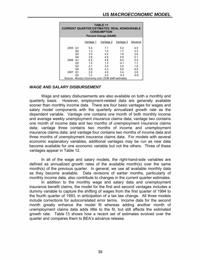
US MACROECONOMIC MODEL
39
TABLE 11 CURRENT QUARTER ESTIMATES: REAL NONDURABLE
CONSUMPTION Percent Change (SAAR)
Vantage 1 Vantage 2 Vantage 3 Advance 2005 Q1 5.5 7.1 5.4 4.9 Q2 1.3 1.5 1.7 3.3 Q3 3.5 4.2 1.6 2.6 Q4 3.8 4.6 5.8 5.1 2006 Q1 6.5 5.8 6.0 5.4 Q2 1.5 1.3 -0.1 1.7 Q3 2.1 3.4 3.0 1.6 Q4 2.8 4.3 5.6 6.9 2007 Q1 2.9 4.9 3.4 2.9 Q2 1.2 2.0 -0.3 -0.8 Source: Moody’s Economy.com; DOB staff estimates.
WAGE AND SALARY DISBURSEMENT Wage and salary disbursements are also available on both a monthly and quarterly basis. However, employment-related data are generally available sooner than monthly income data. There are four basic vantages for wages and salary model components with the quarterly annualized growth rate as the dependent variable. Vantage one contains one month of both monthly income and average weekly unemployment insurance claims data; vantage two contains one month of income data and two months of unemployment insurance claims data; vantage three contains two months of income and unemployment insurance claims data; and vantage four contains two months of income data and three months of unemployment insurance claims data. For models with several economic explanatory variables, additional vantages may be run as new data become available for one economic variable but not the others. Three of these vantages appear in Table 12. In all of the wage and salary models, the right-hand-side variables are defined as annualized growth rates of the available month(s) over the same month(s) of the previous quarter. In general, we use all available monthly data as they become available. Data revisions of earlier months, particularly of monthly income data, also contribute to changes in the current quarter estimates. In addition to the monthly wage and salary data and unemployment insurance benefit claims, the model for the first and second vantages includes a dummy variable to capture the shifting of wages from the first quarter of 1994 to the fourth quarter of 1993, in anticipation of a tax law change. All three models include corrections for autocorrelated error terms. Income data for the second month greatly enhance the model fit whereas adding another month of unemployment claims data adds little to the fit, but still affects the estimated growth rate. Table 13 shows how a recent set of estimates evolved over the quarter and compares them to BEA’s advance release.
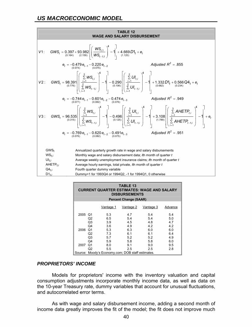
US MACROECONOMIC MODEL
40
TABLE 12 WAGE AND SALARY DISBURSEMENT
,1
(0.164) (2.159) (1.120)1,1
21 2
(0.074) (0.075)
2
,1
2(0.776)1,
1
4
4
1: 0.397 93.982 4.669
0.479 0.220 .855
2 : 98.391
1 1
1
tt t
t
t t t
t ii
t
t ii
tWS
V GWS eWS
e e e Adjusted R
WSV GWS
WS
D−
− −
=
−=
= + + +
= − − =
∑=
∑
⎡ ⎤⎛ ⎞⎢ ⎥−⎜ ⎟⎜ ⎟⎢ ⎥⎝ ⎠⎣ ⎦
⎡ ⎤⎛ ⎞⎢⎜ ⎟⎢ −⎜ ⎟⎢⎜ ⎟⎢⎝ ⎠⎣ ⎦
2
,1
2(0.106) (0.682) (0.234)1,
1
21 2 3
(0.077) (0.082) (0.076)
2
,1
(0.315)
4
0.290 1.332 0.566
0.744 0.601 0.474 .949
3 : 96.535
1 1 4t i
it
t ii
t t t t
t ii
t
t t e
e e e e Adjusted R
WSV GWS
W
UID Q
UI=
−=
− − −
=
∑+ + +
∑
= − − − =
∑=
⎡ ⎤⎛ ⎞⎥ ⎢ ⎥⎜ ⎟⎥ ⎢ ⎥− −⎜ ⎟⎥ ⎢ ⎥⎜ ⎟⎥ ⎢ ⎥⎝ ⎠⎣ ⎦
3 3
, ,1 1
2 3 3(0.125) (1.789)1, 1, 1,
1 1 1
1(0.076) (0.082)
4 4 4
0.496 3.108
0.769 0.620
1 1 1t i t i
i it
t i t i t ii i i
t t t
eS
e e e
UI AHETP
UI AHETP= =
− − −= = =
−
∑ ∑+ +
∑ ∑ ∑
= − −
⎡ ⎤ ⎡ ⎤ ⎡ ⎤⎛ ⎞ ⎛ ⎞ ⎛ ⎞⎢ ⎥ ⎢ ⎥ ⎢ ⎥⎜ ⎟ ⎜ ⎟ ⎜ ⎟⎢ ⎥ ⎢ ⎥ ⎢ ⎥− − − −⎜ ⎟ ⎜ ⎟ ⎜ ⎟⎢ ⎥ ⎢ ⎥ ⎢ ⎥⎜ ⎟ ⎜ ⎟ ⎜ ⎟⎢ ⎥ ⎢ ⎥ ⎢ ⎥⎝ ⎠ ⎝ ⎠ ⎝ ⎠⎣ ⎦ ⎣ ⎦ ⎣ ⎦
22 3
(0.075)0.491 .951te Adjusted R− −− =
GWSt Annualized quarterly growth rate in wage and salary disbursements WSt,i Monthly wage and salary disbursement data; ith month of quarter t UIt,i Average weekly unemployment insurance claims; ith month of quarter t AHETPt,i Average hourly earnings, total private, ith month of quarter t Q4t,i Fourth quarter dummy variable D1t,i Dummy=1 for 1993Q4 or 1994Q2, -1 for 1994Q1, 0 otherwise
TABLE 13
CURRENT QUARTER ESTIMATES: WAGE AND SALARY DISBURSEMENTS
Percent Change (SAAR) Vantage 1 Vantage 2 Vantage 3 Advance
2005 Q1 5.3 4.7 5.4 5.4 Q2 6.5 5.4 5.4 5.0 Q3 3.9 4.5 4.8 4.7 Q4 3.6 4.9 4.2 4.2
2006 Q1 5.3 6.3 6.0 6.0 Q2 7.3 6.1 6.1 6.4 Q3 5.7 5.2 5.2 4.9 Q4 5.9 5.8 5.8 6.0
2007 Q1 8.0 9.1 9.0 9.5 Q2 5.5 2.5 2.5 2.8
Source: Moody’s Economy.com; DOB staff estimates.
PROPRIETORS’ INCOME Models for proprietors' income with the inventory valuation and capital consumption adjustments incorporate monthly income data, as well as data on the 10-year Treasury rate, dummy variables that account for unusual fluctuations, and autocorrelated error terms. As with wage and salary disbursement income, adding a second month of income data greatly improves the fit of the model; the fit does not improve much
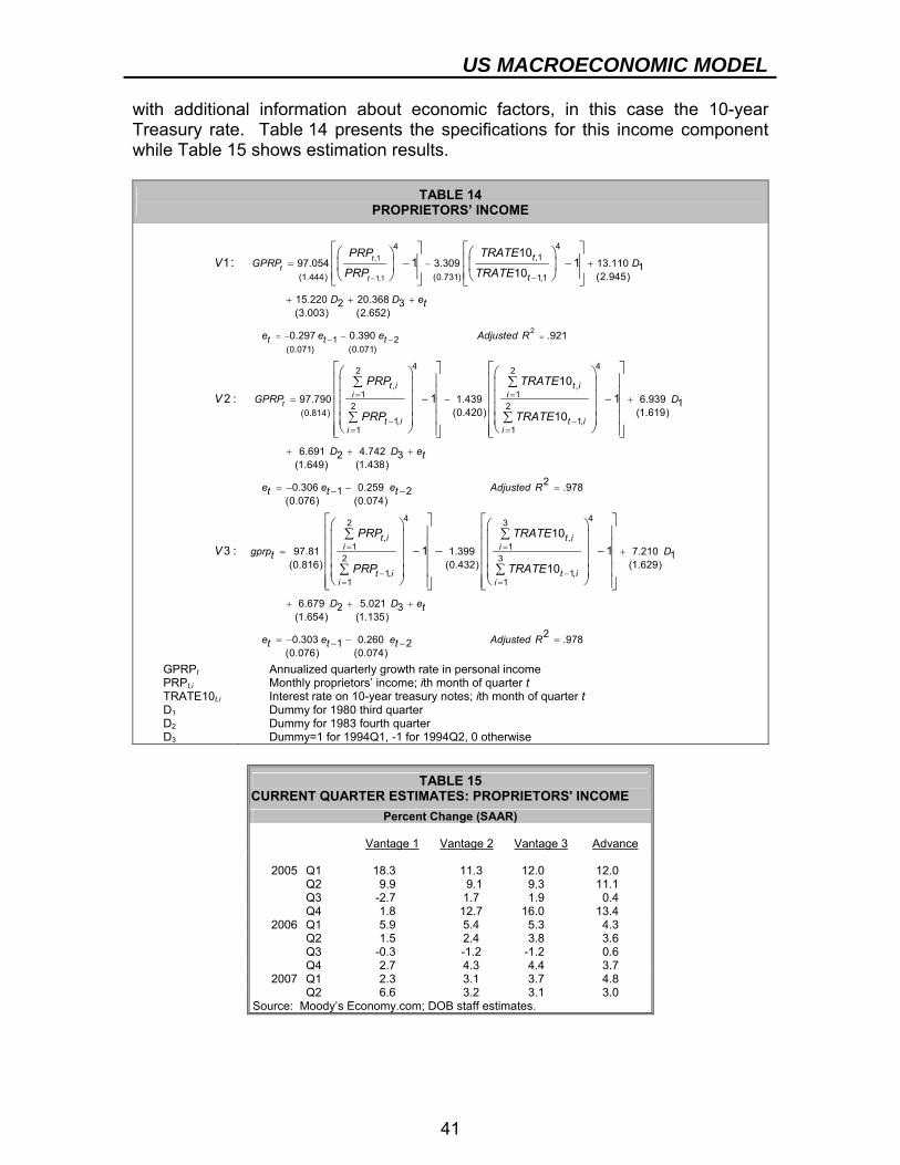
US MACROECONOMIC MODEL
41
with additional information about economic factors, in this case the 10-year Treasury rate. Table 14 presents the specifications for this income component while Table 15 shows estimation results.
TABLE 14 PROPRIETORS’ INCOME
,1
1,1
44,1
(1.444) (0.731) 1,1
1 2(0.071) (0.071)
97.054 3.309 13.110 1(2.945)
15.220 20.3682 3(3.003) (2.652)
0.297 0.390
101 1 1
10: t
tt
t
t
t t t
GPRP D
D D et
e e e Adjuste
TRATEPRPV
PRP TRATE−
−
−
= − −− −
= +
+ + +
− −⎡ ⎤⎡ ⎤ ⎛ ⎞⎛ ⎞ ⎢ ⎥⎢ ⎥ ⎜ ⎟⎜ ⎟⎢ ⎥⎢ ⎥⎝ ⎠ ⎝ ⎠⎣ ⎦ ⎣ ⎦
2
4 42 2
, ,1 1
2 2(0.814)
1, 1,1 1
.921
97.790 1.439 6.939 1(0.420) (1.619)
6.691 4.7422(1.438)(1.649)
102 : 1 1
10t
t i t ii i
t i t ii i
d R
GPRP D
D
PRP TRATEV
PRP TRATE
=
= =
− −= =
= − +
+ +
− −
⎡ ⎤ ⎡ ⎤⎛ ⎞ ⎛ ⎞⎢ ⎥ ⎢ ⎥∑ ∑⎜ ⎟ ⎜ ⎟⎢ ⎥ ⎢ ⎥⎜ ⎟ ⎜ ⎟⎢ ⎥ ⎢ ⎥⎜ ⎟ ⎜ ⎟∑ ∑⎢ ⎥ ⎢ ⎥⎜ ⎟ ⎜ ⎟⎝ ⎠ ⎝ ⎠⎢ ⎥ ⎢ ⎥⎣ ⎦ ⎣ ⎦
4 42 3
, ,1 1
2 3
1, 1,1 1
3
20.306 0.259 .9781 2(0.076) (0.074)
97.81 1.399(0.816) (0.432)
103 : 1 1
10
t i t ii i
t i t ii i
D et
e e e Adjusted Rt t t
gprpt
PRP TRATEV
PRP TRATE
= =
− −= =
+
= − − =− −
= − −
⎡ ⎤ ⎡ ⎤⎛ ⎞ ⎛ ⎞⎢ ⎥ ⎢∑ ∑⎜ ⎟ ⎜ ⎟⎢ ⎥ ⎢⎜ ⎟ ⎜ ⎟−⎢ ⎥ ⎢⎜ ⎟ ⎜ ⎟∑ ∑⎢ ⎥ ⎢⎜ ⎟ ⎜ ⎟⎝ ⎠ ⎝ ⎠⎢ ⎥ ⎢⎣ ⎦ ⎣ ⎦
7.210 1(1.629)
6.679 5.0212 3(1.654) (1.135)
20.303 0.260 .9781 2(0.076) (0.074)
D
D D et
e e e Adjusted Rt t t
+
+ + +
= − − =− −
⎥⎥⎥⎥⎥
GPRPt Annualized quarterly growth rate in personal income PRPt,i Monthly proprietors’ income; ith month of quarter t TRATE10t,i Interest rate on 10-year treasury notes; ith month of quarter t D1 Dummy for 1980 third quarter D2 Dummy for 1983 fourth quarter D3 Dummy=1 for 1994Q1, -1 for 1994Q2, 0 otherwise
TABLE 15
CURRENT QUARTER ESTIMATES: PROPRIETORS' INCOME Percent Change (SAAR)
Vantage 1 Vantage 2 Vantage 3 Advance
2005 Q1 18.3 11.3 12.0 12.0
Q2 9.9 9.1 9.3 11.1 Q3 -2.7 1.7 1.9 0.4 Q4 1.8 12.7 16.0 13.4
2006 Q1 5.9 5.4 5.3 4.3 Q2 1.5 2.4 3.8 3.6 Q3 -0.3 -1.2 -1.2 0.6 Q4 2.7 4.3 4.4 3.7
2007 Q1 2.3 3.1 3.7 4.8 Q2 6.6 3.2 3.1 3.0
Source: Moody’s Economy.com; DOB staff estimates.
US MACROECONOMIC MODEL
42
FORECAST ACCURACY SELECTED VARIABLES Forecasting the future of the economy is very difficult, due not only to the issues discussed above, but also to the occurrence of economic shocks, i.e., unpredictable events such as the September 11 attacks or the hurricanes that recently hit the Gulf Coast. Predicting business cycle turning points is a particularly difficult challenge for forecasters since the model coefficients, on which future predictions are based, are fixed at values that summarize the entire history of the data. For example, at the end of 2000, DOB predicted that the economy would experience a significant slowdown for the following year. However, we could not predict the events of September 11. On the other hand, we projected that the impact of September 11 would be less severe, but longer lasting than it turned out to be. Here we select a few key economic variables and compare our one-year-ahead annual forecast to the initial BEA and BLS estimates.10 For comparison purposes, we also include the Blue Chip forecast where available. As the following figures indicate, when the economy is on a steady growth path, the forecast errors tend to be smaller than when the economy actually changes direction. For both real U.S. GDP and inflation, DOB's forecast has tended to be very similar to the Blue Chip Consensus forecast. Like the Blue Chip consensus forecast, DOB overestimated the strength of real U.S. GDP during the 2001 recession, but underestimated strength of the economy coming out. In contrast, because of the unusually long period with which the U.S. labor market recovery lagged the recovery in output, there was a tendency to overpredict employment in 2002 and 2003 and income in 2003.
10 We use the initial estimates rather than the most recent estimates as benchmarks to assess DOB’s forecast accuracy since it would be impossible to forecast future revisions to the data.
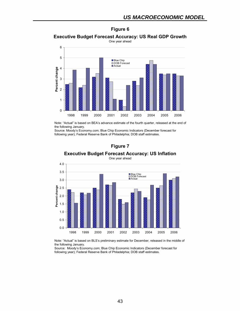
US MACROECONOMIC MODEL
43
Figure 6
0
1
2
3
4
5
6
1998 1999 2000 2001 2002 2003 2004 2005 2006
Perc
ent c
hang
eBlue ChipDOB ForecastActual
Executive Budget Forecast Accuracy: US Real GDP GrowthOne year ahead
Note: “Actual” is based on BEA’s advance estimate of the fourth quarter, released at the end of the following January. Source: Moody’s Economy.com; Blue Chip Economic Indicators (December forecast for following year); Federal Reserve Bank of Philadelphia; DOB staff estimates.
Figure 7
0.0
0.5
1.0
1.5
2.0
2.5
3.0
3.5
4.0
1998 1999 2000 2001 2002 2003 2004 2005 2006
Perc
ent c
hang
e
Blue ChipDOB ForecastActual
Executive Budget Forecast Accuracy: US InflationOne year ahead
Note: “Actual” is based on BLS’s preliminary estimate for December, released in the middle of the following January.Source: Moody’s Economy.com; Blue Chip Economic Indicators (December forecast for following year); Federal Reserve Bank of Philadelphia; DOB staff estimates.
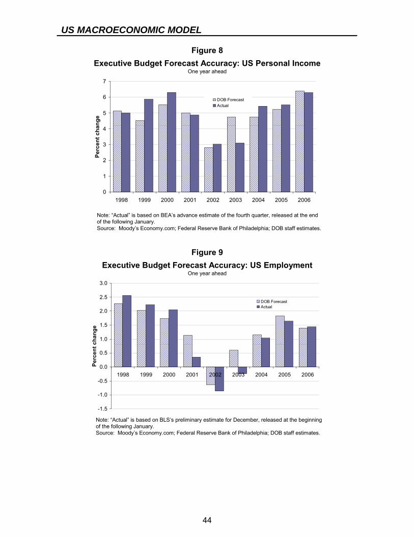
US MACROECONOMIC MODEL
44
Figure 8
0
1
2
3
4
5
6
7
1998 1999 2000 2001 2002 2003 2004 2005 2006
Perc
ent c
hang
eDOB ForecastActual
Executive Budget Forecast Accuracy: US Personal IncomeOne year ahead
Note: “Actual” is based on BEA’s advance estimate of the fourth quarter, released at the end of the following January. Source: Moody’s Economy.com; Federal Reserve Bank of Philadelphia; DOB staff estimates.
Figure 9
-1.5
-1.0
-0.5
0.0
0.5
1.0
1.5
2.0
2.5
3.0
1998 1999 2000 2001 2002 2003 2004 2005 2006
Perc
ent c
hang
e
DOB ForecastActual
Executive Budget Forecast Accuracy: US EmploymentOne year ahead
Note: “Actual” is based on BLS’s preliminary estimate for December, released at the beginning of the following January. Source: Moody’s Economy.com; Federal Reserve Bank of Philadelphia; DOB staff estimates.
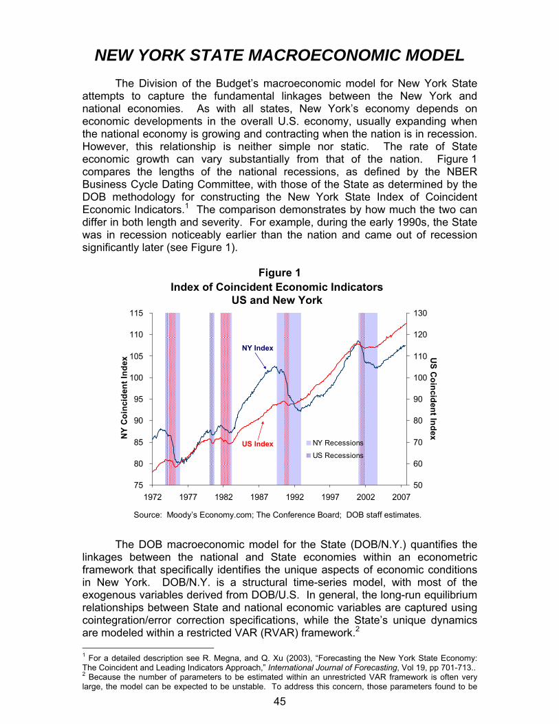
45
NEW YORK STATE MACROECONOMIC MODEL The Division of the Budget’s macroeconomic model for New York State attempts to capture the fundamental linkages between the New York and national economies. As with all states, New York’s economy depends on economic developments in the overall U.S. economy, usually expanding when the national economy is growing and contracting when the nation is in recession. However, this relationship is neither simple nor static. The rate of State economic growth can vary substantially from that of the nation. Figure 1 compares the lengths of the national recessions, as defined by the NBER Business Cycle Dating Committee, with those of the State as determined by the DOB methodology for constructing the New York State Index of Coincident Economic Indicators.1 The comparison demonstrates by how much the two can differ in both length and severity. For example, during the early 1990s, the State was in recession noticeably earlier than the nation and came out of recession significantly later (see Figure 1).
Figure 1
75
80
85
90
95
100
105
110
115
1972 1977 1982 1987 1992 1997 2002 2007
NY
Coi
ncid
ent I
ndex
50
60
70
80
90
100
110
120
130
US C
oincident Index
NY Recessions
US Recessions
Index of Coincident Economic IndicatorsUS and New York
Source: Moody’s Economy.com; The Conference Board; DOB staff estimates.
US Index
NY Index
The DOB macroeconomic model for the State (DOB/N.Y.) quantifies the linkages between the national and State economies within an econometric framework that specifically identifies the unique aspects of economic conditions in New York. DOB/N.Y. is a structural time-series model, with most of the exogenous variables derived from DOB/U.S. In general, the long-run equilibrium relationships between State and national economic variables are captured using cointegration/error correction specifications, while the State’s unique dynamics are modeled within a restricted VAR (RVAR) framework.2 1 For a detailed description see R. Megna, and Q. Xu (2003), “Forecasting the New York State Economy: The Coincident and Leading Indicators Approach,” International Journal of Forecasting, Vol 19, pp 701-713.. 2 Because the number of parameters to be estimated within an unrestricted VAR framework is often very large, the model can be expected to be unstable. To address this concern, those parameters found to be
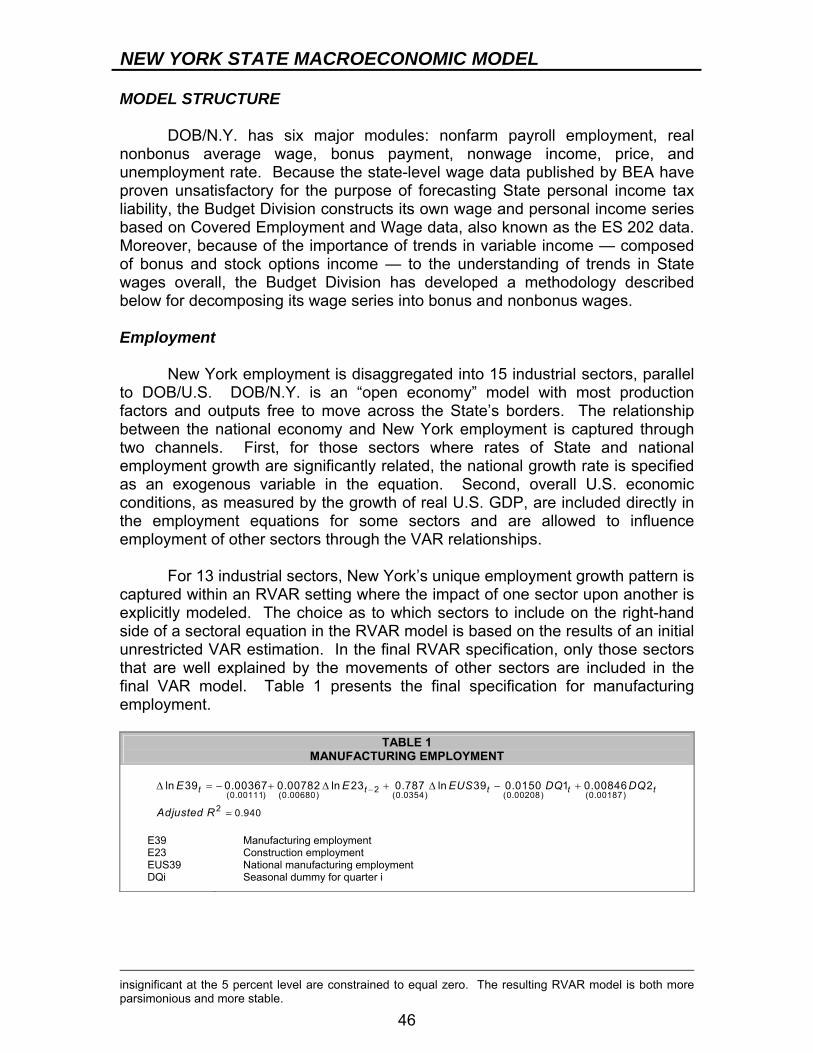
NEW YORK STATE MACROECONOMIC MODEL
46
MODEL STRUCTURE DOB/N.Y. has six major modules: nonfarm payroll employment, real nonbonus average wage, bonus payment, nonwage income, price, and unemployment rate. Because the state-level wage data published by BEA have proven unsatisfactory for the purpose of forecasting State personal income tax liability, the Budget Division constructs its own wage and personal income series based on Covered Employment and Wage data, also known as the ES 202 data. Moreover, because of the importance of trends in variable income — composed of bonus and stock options income — to the understanding of trends in State wages overall, the Budget Division has developed a methodology described below for decomposing its wage series into bonus and nonbonus wages. Employment New York employment is disaggregated into 15 industrial sectors, parallel to DOB/U.S. DOB/N.Y. is an “open economy” model with most production factors and outputs free to move across the State’s borders. The relationship between the national economy and New York employment is captured through two channels. First, for those sectors where rates of State and national employment growth are significantly related, the national growth rate is specified as an exogenous variable in the equation. Second, overall U.S. economic conditions, as measured by the growth of real U.S. GDP, are included directly in the employment equations for some sectors and are allowed to influence employment of other sectors through the VAR relationships. For 13 industrial sectors, New York’s unique employment growth pattern is captured within an RVAR setting where the impact of one sector upon another is explicitly modeled. The choice as to which sectors to include on the right-hand side of a sectoral equation in the RVAR model is based on the results of an initial unrestricted VAR estimation. In the final RVAR specification, only those sectors that are well explained by the movements of other sectors are included in the final VAR model. Table 1 presents the final specification for manufacturing employment.
TABLE 1 MANUFACTURING EMPLOYMENT
2(0.00111) (0.00680) (0.0354) (0.00208) (0.00187)
2 0.940
ln 39 0.00367 0.00782 ln 23 0.787 ln 39 0.0150 1 0.00846 2t t t t tE E EUS DQ DQ
Adjusted R
−Δ = − + Δ + Δ − +
=
E39 Manufacturing employment E23 Construction employment EUS39 National manufacturing employment DQi Seasonal dummy for quarter i
insignificant at the 5 percent level are constrained to equal zero. The resulting RVAR model is both more parsimonious and more stable.
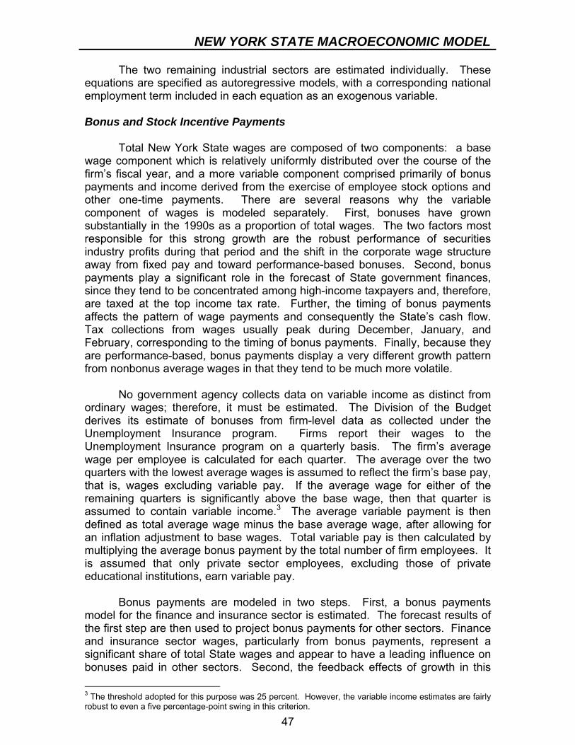
NEW YORK STATE MACROECONOMIC MODEL
47
The two remaining industrial sectors are estimated individually. These equations are specified as autoregressive models, with a corresponding national employment term included in each equation as an exogenous variable. Bonus and Stock Incentive Payments Total New York State wages are composed of two components: a base wage component which is relatively uniformly distributed over the course of the firm’s fiscal year, and a more variable component comprised primarily of bonus payments and income derived from the exercise of employee stock options and other one-time payments. There are several reasons why the variable component of wages is modeled separately. First, bonuses have grown substantially in the 1990s as a proportion of total wages. The two factors most responsible for this strong growth are the robust performance of securities industry profits during that period and the shift in the corporate wage structure away from fixed pay and toward performance-based bonuses. Second, bonus payments play a significant role in the forecast of State government finances, since they tend to be concentrated among high-income taxpayers and, therefore, are taxed at the top income tax rate. Further, the timing of bonus payments affects the pattern of wage payments and consequently the State’s cash flow. Tax collections from wages usually peak during December, January, and February, corresponding to the timing of bonus payments. Finally, because they are performance-based, bonus payments display a very different growth pattern from nonbonus average wages in that they tend to be much more volatile. No government agency collects data on variable income as distinct from ordinary wages; therefore, it must be estimated. The Division of the Budget derives its estimate of bonuses from firm-level data as collected under the Unemployment Insurance program. Firms report their wages to the Unemployment Insurance program on a quarterly basis. The firm’s average wage per employee is calculated for each quarter. The average over the two quarters with the lowest average wages is assumed to reflect the firm’s base pay, that is, wages excluding variable pay. If the average wage for either of the remaining quarters is significantly above the base wage, then that quarter is assumed to contain variable income.3 The average variable payment is then defined as total average wage minus the base average wage, after allowing for an inflation adjustment to base wages. Total variable pay is then calculated by multiplying the average bonus payment by the total number of firm employees. It is assumed that only private sector employees, excluding those of private educational institutions, earn variable pay. Bonus payments are modeled in two steps. First, a bonus payments model for the finance and insurance sector is estimated. The forecast results of the first step are then used to project bonus payments for other sectors. Finance and insurance sector wages, particularly from bonus payments, represent a significant share of total State wages and appear to have a leading influence on bonuses paid in other sectors. Second, the feedback effects of growth in this 3 The threshold adopted for this purpose was 25 percent. However, the variable income estimates are fairly robust to even a five percentage-point swing in this criterion.
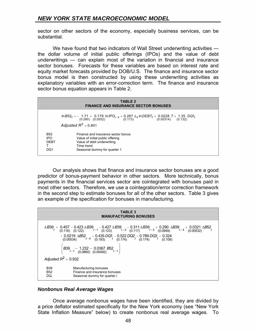
NEW YORK STATE MACROECONOMIC MODEL
48
sector on other sectors of the economy, especially business services, can be substantial. We have found that two indicators of Wall Street underwriting activities — the dollar volume of initial public offerings (IPOs) and the value of debt underwritings — can explain most of the variation in financial and insurance sector bonuses. Forecasts for these variables are based on interest rate and equity market forecasts provided by DOB/U.S. The finance and insurance sector bonus model is then constructed by using these underwriting activities as explanatory variables with an error-correction term. The finance and insurance sector bonus equation appears in Table 2.
TABLE 2 FINANCE AND INSURANCE SECTOR BONUSES
4 4
(0.280) (0.0552) (0.173) (0.00314) (0.132)2
ln 52 1.71 0.179 ln 0.267 ln 0.0228 1.35 1
0.801
t tt tB IPO DEBT T DQ
Adjusted R
−= − + + Δ + +
=
B52 Finance and insurance sector bonus IPO Value of initial public offering DEBT Value of debt underwriting T Time trend DQ1 Seasonal dummy for quarter 1
Our analysis shows that finance and insurance sector bonuses are a good predictor of bonus-payment behavior in other sectors. More technically, bonus payments in the financial services sector are cointegrated with bonuses paid in most other sectors. Therefore, we use a cointegration/error correction framework in the second step to estimate bonuses for all of the other sectors. Table 3 gives an example of the specification for bonuses in manufacturing.
TABLE 3 MANUFACTURING BONUSES
- 1 - 2 - 3 - 4
- 4
(0.116) (0.122) (0.123) (0.117) (0.0949) (0.00532)
(0.00534) (0.193) (0.174) (0.174)
39 0.457 0.423 39 0.427 39 0.311 39 0.290 39 0.0321 52
- 0.0219 52 0.435 1 0.522 2 0.789 3 0.324t t t t t t
t t t t
B B B B B B
B DQ DQ DQ
= − − − + +
−
Δ Δ Δ Δ Δ Δ
Δ − − −
- 1 - 1
(0.109)
(0.0860) (0.00492)
2
39 1.232 0.0367 52
0.932
t tB B
Adjusted R
⎛ ⎞⎜ ⎟⎜ ⎟⎝ ⎠
− −
=
B39 Manufacturing bonuses B52 Finance and insurance bonuses DQi Seasonal dummy for quarter i
Nonbonus Real Average Wages Once average nonbonus wages have been identified, they are divided by a price deflator estimated specifically for the New York economy (see “New York State Inflation Measure” below) to create nonbonus real average wages. To
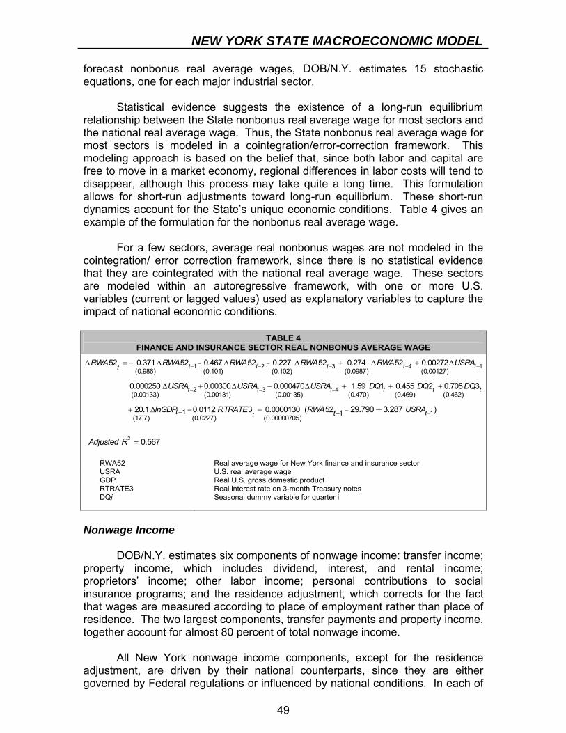
NEW YORK STATE MACROECONOMIC MODEL
49
forecast nonbonus real average wages, DOB/N.Y. estimates 15 stochastic equations, one for each major industrial sector. Statistical evidence suggests the existence of a long-run equilibrium relationship between the State nonbonus real average wage for most sectors and the national real average wage. Thus, the State nonbonus real average wage for most sectors is modeled in a cointegration/error-correction framework. This modeling approach is based on the belief that, since both labor and capital are free to move in a market economy, regional differences in labor costs will tend to disappear, although this process may take quite a long time. This formulation allows for short-run adjustments toward long-run equilibrium. These short-run dynamics account for the State’s unique economic conditions. Table 4 gives an example of the formulation for the nonbonus real average wage. For a few sectors, average real nonbonus wages are not modeled in the cointegration/ error correction framework, since there is no statistical evidence that they are cointegrated with the national real average wage. These sectors are modeled within an autoregressive framework, with one or more U.S. variables (current or lagged values) used as explanatory variables to capture the impact of national economic conditions.
TABLE 4 FINANCE AND INSURANCE SECTOR REAL NONBONUS AVERAGE WAGE
1 2 3 4 1
2 3 4
(0.986) (0.101) (0.102) (0.0987) (0.00127)
(0.00133) (0.00131) (0.00135)
52 0.371 52 0.467 52 0.227 52 0.274 52 0.00272
0.000250 0.00300 0.000470 1
t t t t t
t t t
tRWA RWA RWA RWA RWA USRA
USRA USRA USRA
− −− − − − −
− − −
Δ = − Δ Δ Δ + Δ + Δ
Δ + Δ − Δ +
2
1
(0.470) (0.469) (0.462)
1(17.7) (0.0227) (0.00000705)
1
.59 1 0.455 2 0.705 3
20.1 0.0112 3 0.0000130 ( 52 )29.790 3.287
0.567
t
t t t
tt t
DQ DQ DQ
lnGDP RTRATE RWA USRA
Adjusted R
− −− −
+ +
+ Δ − −
=
−
RWA52 Real average wage for New York finance and insurance sector USRA U.S. real average wage GDP Real U.S. gross domestic product RTRATE3 Real interest rate on 3-month Treasury notes DQi
Seasonal dummy variable for quarter i
Nonwage Income DOB/N.Y. estimates six components of nonwage income: transfer income; property income, which includes dividend, interest, and rental income; proprietors’ income; other labor income; personal contributions to social insurance programs; and the residence adjustment, which corrects for the fact that wages are measured according to place of employment rather than place of residence. The two largest components, transfer payments and property income, together account for almost 80 percent of total nonwage income. All New York nonwage income components, except for the residence adjustment, are driven by their national counterparts, since they are either governed by Federal regulations or influenced by national conditions. In each of
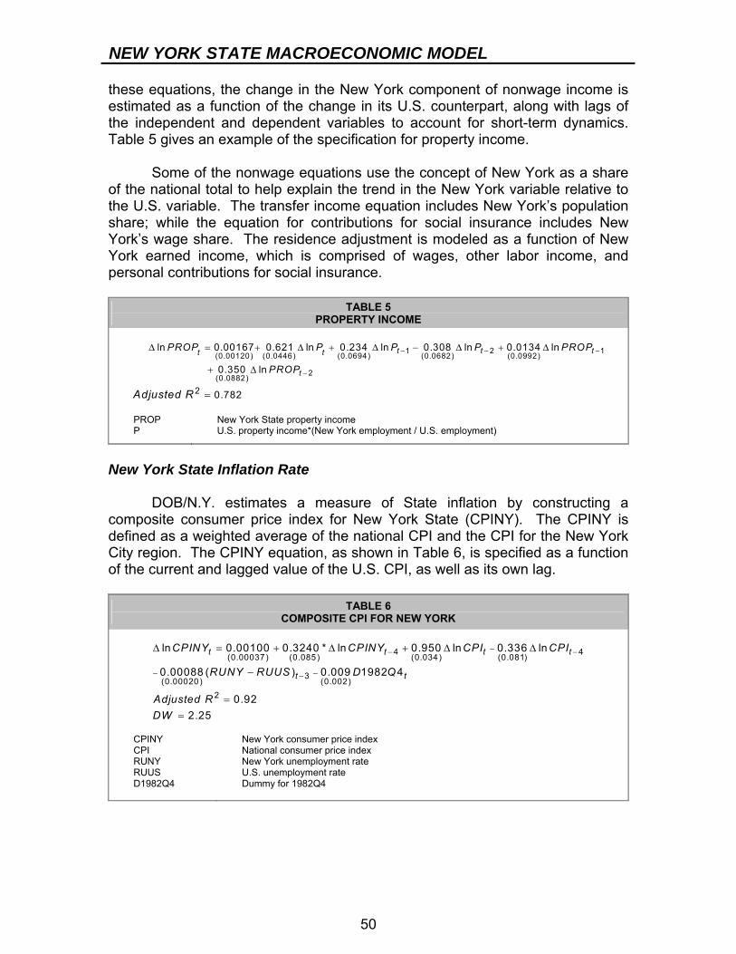
NEW YORK STATE MACROECONOMIC MODEL
50
these equations, the change in the New York component of nonwage income is estimated as a function of the change in its U.S. counterpart, along with lags of the independent and dependent variables to account for short-term dynamics. Table 5 gives an example of the specification for property income. Some of the nonwage equations use the concept of New York as a share of the national total to help explain the trend in the New York variable relative to the U.S. variable. The transfer income equation includes New York’s population share; while the equation for contributions for social insurance includes New York’s wage share. The residence adjustment is modeled as a function of New York earned income, which is comprised of wages, other labor income, and personal contributions for social insurance.
TABLE 5 PROPERTY INCOME
t t tt t
t
PROP P P P PROP
PROP
Adjusted R
1 2 1(0.00120) (0.0446) (0.0694) (0.0682) (0.0992)
2(0.0882)
2
ln 0.00167 0.621 ln 0.234 ln 0.308 ln 0.0134 ln
0.350 ln
0.782
− − −
−
Δ = + Δ + Δ − Δ + Δ
+ Δ
=
PROP New York State property income P U.S. property income*(New York employment / U.S. employment)
New York State Inflation Rate DOB/N.Y. estimates a measure of State inflation by constructing a composite consumer price index for New York State (CPINY). The CPINY is defined as a weighted average of the national CPI and the CPI for the New York City region. The CPINY equation, as shown in Table 6, is specified as a function of the current and lagged value of the U.S. CPI, as well as its own lag.
TABLE 6 COMPOSITE CPI FOR NEW YORK
−− −
− −−
Δ = + Δ + Δ Δ
−
==
4 4(0.00037) (0.085) (0.034) (0.081)
3(0.00020) (0.002)2
ln 0.00100 0.3240 * ln 0.950 ln 0.336 ln
0.00088 ( ) 0.009 1982 4
0.922.25
t t t t
t t
CPINY CPINY CPI CPI
RUNY RUUS D Q
Adjusted RDW
CPINY New York consumer price index CPI RUNY RUUS D1982Q4
National consumer price index New York unemployment rate U.S. unemployment rate Dummy for 1982Q4
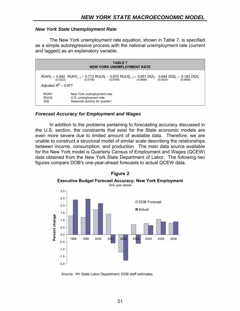
NEW YORK STATE MACROECONOMIC MODEL
51
New York State Unemployment Rate The New York unemployment rate equation, shown in Table 7, is specified as a simple autoregressive process with the national unemployment rate (current and lagged) as an explanatory variable.
TABLE 7 NEW YORK UNEMPLOYMENT RATE
t t t t t t tRUNY RUNY RUUS RUUS DQ DQ DQ
Adjusted R
1 1(0.0222) (0.0738) (0.0769) (0.0609) (0.0624) (0.0609)2
0.942 0.713 0.670 0.851 1 0.644 2 0.183 3
0.977
−− −= + − + +
=
RUNY New York unemployment rate RUUS U.S. unemployment rate DQi Seasonal dummy for quarter i
Forecast Accuracy for Employment and Wages In addition to the problems pertaining to forecasting accuracy discussed in the U.S. section, the constraints that exist for the State economic models are even more severe due to limited amount of available data. Therefore, we are unable to construct a structural model of similar scale describing the relationships between income, consumption, and production. The main data source available for the New York model is Quarterly Census of Employment and Wages (QCEW) data obtained from the New York State Department of Labor. The following two figures compare DOB's one-year-ahead forecasts to actual QCEW data.
Figure 2
-2.0
-1.5
-1.0
-0.5
0.0
0.5
1.0
1.5
2.0
2.5
3.0
1998 1999 2000 2001 2002 2003 2004 2005 2006Perc
ent c
hang
e
DOB Forecast
Actual
Executive Budget Forecast Accuracy: New York EmploymentOne year ahead
Source: NY State Labor Department; DOB staff estimates.
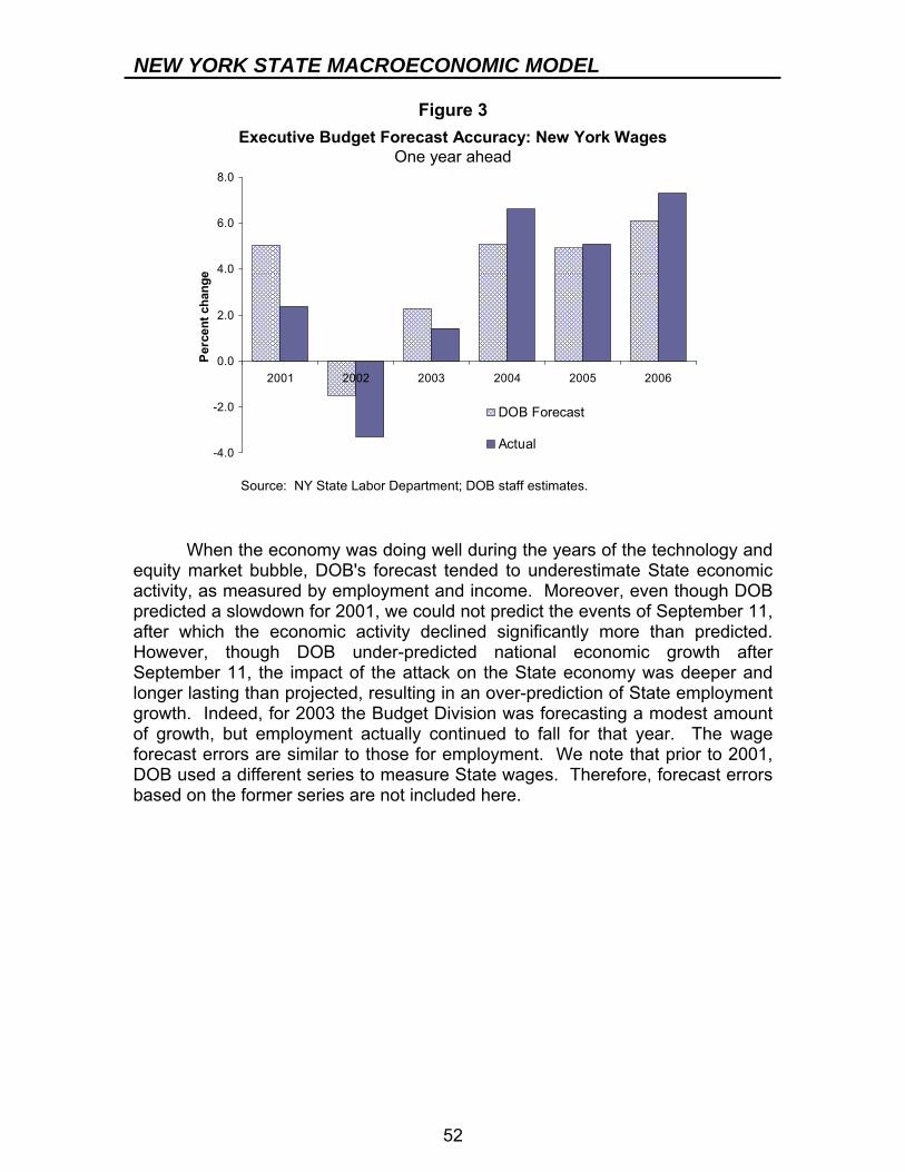
NEW YORK STATE MACROECONOMIC MODEL
52
Figure 3
-4.0
-2.0
0.0
2.0
4.0
6.0
8.0
2001 2002 2003 2004 2005 2006
Perc
ent c
hang
e
DOB Forecast
Actual
Executive Budget Forecast Accuracy: New York WagesOne year ahead
Source: NY State Labor Department; DOB staff estimates.
When the economy was doing well during the years of the technology and equity market bubble, DOB's forecast tended to underestimate State economic activity, as measured by employment and income. Moreover, even though DOB predicted a slowdown for 2001, we could not predict the events of September 11, after which the economic activity declined significantly more than predicted. However, though DOB under-predicted national economic growth after September 11, the impact of the attack on the State economy was deeper and longer lasting than projected, resulting in an over-prediction of State employment growth. Indeed, for 2003 the Budget Division was forecasting a modest amount of growth, but employment actually continued to fall for that year. The wage forecast errors are similar to those for employment. We note that prior to 2001, DOB used a different series to measure State wages. Therefore, forecast errors based on the former series are not included here.
53
NEW YORK STATE ADJUSTED GROSS INCOME Annual data pertaining to the number of tax returns and the components of New York State adjusted gross income (NYSAGI) are obtained from samples taken from the State taxpayer population by the New York State Department of Taxation and Finance. Single-equation econometric models are used to project the future number of returns, as well as all the components of income except for the largest component, wages. To ensure consistency with DOB’s New York economic forecast, the forecast growth rate for State wages and salaries derived from DOB/N.Y. is applied to the wage base obtained from the taxpayer sample. In almost all cases, the data series on the components of NYSAGI are found to be nonstationary. Therefore, to avoid being misled by spurious regression results, a logarithmic transformation is performed and then first-differenced for all series for which at least 20 observations are available. Shorter series are modeled in levels. In constructing the sample, the Department of Taxation and Finance tries to capture as accurately as possible the characteristics of the State taxpayer population. However, it is unreasonable to expect that every component of income will be perfectly represented for each and every year. Dummy variables are incorporated into models where anomalies in the data are thought to be the product of sampling error. Detailed descriptions of the models for the number of returns and for the major components of NYSAGI, other than wages, are presented below. All estimation results presented below are based on tax return data from a sample of State taxpayers through the 2005 tax year, made available by the New York State Department of Taxation and Finance. TAX RETURNS The number of tax returns is expected to vary with the number of households that earn any kind of income during the year. The number of such households, in turn, should be closely associated with the number of individuals who are either self-employed, employed by others, or earn taxable income from a source other than labor. Since most taxable income is earned as wages and salaries and thus related to employment, total State payroll employment, which is forecast within DOB/N.Y., is a key input to this model. New Yorkers can earn taxable income from sources other than payroll employment, such as self-employment and real and financial assets. Self-employment is expected to be closely related to proprietors’ income, a component of the NIPA definition of State personal income that is available from BEA and forecast within DOB/N.Y. Another component of personal income that is forecast within DOB/N.Y., State property income, includes interest, dividend, and rental income. The DOB tax return model incorporates the sum of proprietors’ and property income for New York, deflated by the consumer price index for New York as constructed by DOB. A one-time upward shift in the number of tax returns is observed in 1987, believed to be related to the Tax Reform Act of 1986. Beginning in 1987, the
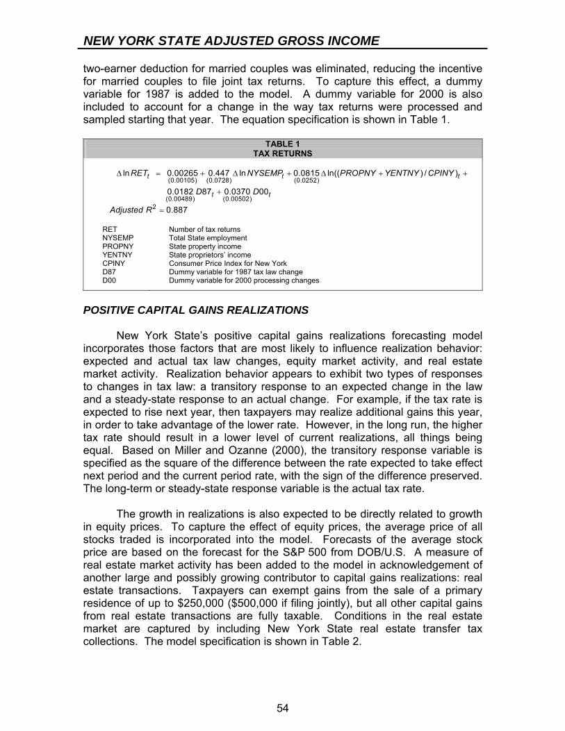
NEW YORK STATE ADJUSTED GROSS INCOME
54
two-earner deduction for married couples was eliminated, reducing the incentive for married couples to file joint tax returns. To capture this effect, a dummy variable for 1987 is added to the model. A dummy variable for 2000 is also included to account for a change in the way tax returns were processed and sampled starting that year. The equation specification is shown in Table 1.
TABLE 1 TAX RETURNS
(0.00105) (0.0728) (0.0252)
(0.00489) (0.00502)2
ln 0.00265 0.447 ln 0.0815 ln(( ) / )
0.0182 87 0.0370 00
0.887
t t t
t t
RET NYSEMP PROPNY YENTNY CPINY
D D
Adjusted R
Δ = + Δ + Δ + +
+
=
RET Number of tax returns NYSEMP Total State employment PROPNY State property income YENTNY State proprietors’ income CPINY Consumer Price Index for New York D87 Dummy variable for 1987 tax law change D00 Dummy variable for 2000 processing changes
POSITIVE CAPITAL GAINS REALIZATIONS New York State’s positive capital gains realizations forecasting model incorporates those factors that are most likely to influence realization behavior: expected and actual tax law changes, equity market activity, and real estate market activity. Realization behavior appears to exhibit two types of responses to changes in tax law: a transitory response to an expected change in the law and a steady-state response to an actual change. For example, if the tax rate is expected to rise next year, then taxpayers may realize additional gains this year, in order to take advantage of the lower rate. However, in the long run, the higher tax rate should result in a lower level of current realizations, all things being equal. Based on Miller and Ozanne (2000), the transitory response variable is specified as the square of the difference between the rate expected to take effect next period and the current period rate, with the sign of the difference preserved. The long-term or steady-state response variable is the actual tax rate. The growth in realizations is also expected to be directly related to growth in equity prices. To capture the effect of equity prices, the average price of all stocks traded is incorporated into the model. Forecasts of the average stock price are based on the forecast for the S&P 500 from DOB/U.S. A measure of real estate market activity has been added to the model in acknowledgement of another large and possibly growing contributor to capital gains realizations: real estate transactions. Taxpayers can exempt gains from the sale of a primary residence of up to $250,000 ($500,000 if filing jointly), but all other capital gains from real estate transactions are fully taxable. Conditions in the real estate market are captured by including New York State real estate transfer tax collections. The model specification is shown in Table 2.
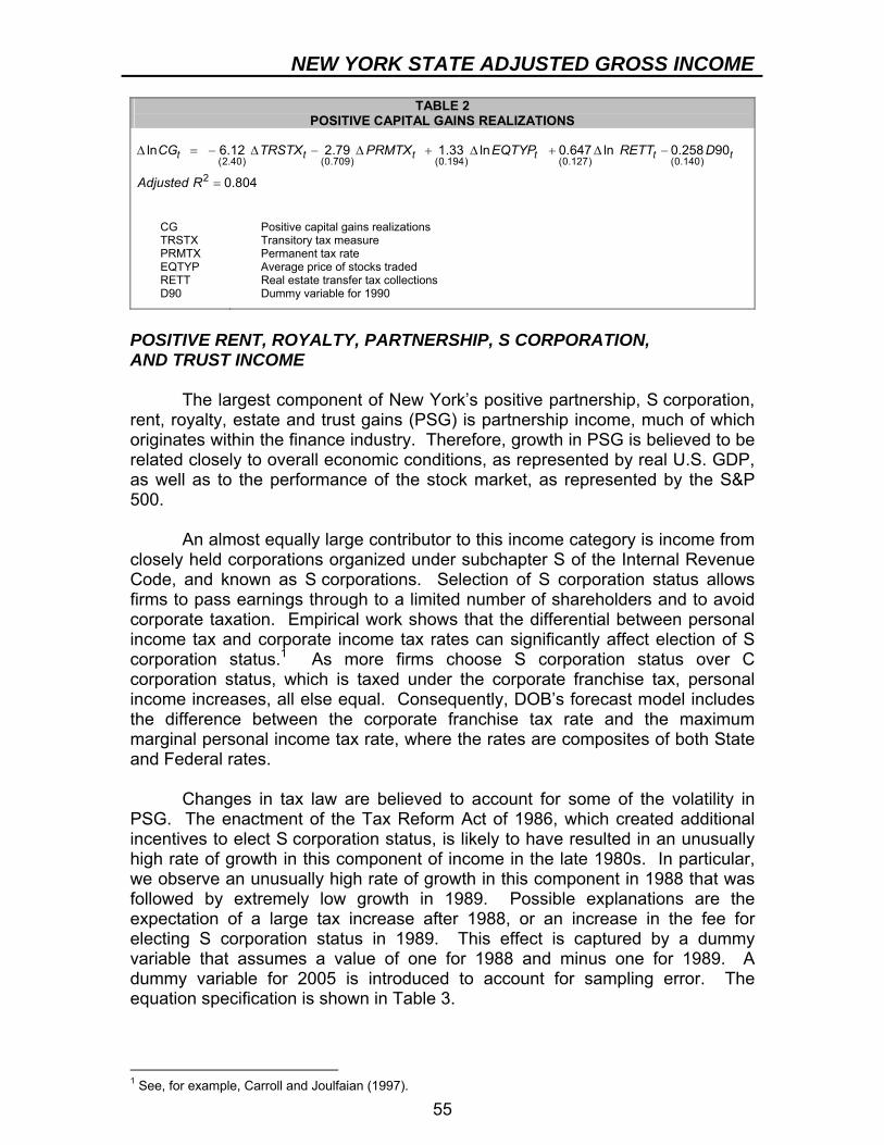
NEW YORK STATE ADJUSTED GROSS INCOME
55
TABLE 2 POSITIVE CAPITAL GAINS REALIZATIONS
(2.40) (0.709) (0.194) (0.127) (0.140)2
ln 6.12 2.79 1.33 ln 0.647 ln 0.258 90
0.804
t t t t t tCG TRSTX PRMTX EQTYP RETT D
Adjusted R
Δ = − Δ − Δ + Δ + Δ −
=
CG Positive capital gains realizations TRSTX Transitory tax measure PRMTX Permanent tax rate EQTYP Average price of stocks traded RETT Real estate transfer tax collections D90 Dummy variable for 1990
POSITIVE RENT, ROYALTY, PARTNERSHIP, S CORPORATION, AND TRUST INCOME The largest component of New York’s positive partnership, S corporation, rent, royalty, estate and trust gains (PSG) is partnership income, much of which originates within the finance industry. Therefore, growth in PSG is believed to be related closely to overall economic conditions, as represented by real U.S. GDP, as well as to the performance of the stock market, as represented by the S&P 500. An almost equally large contributor to this income category is income from closely held corporations organized under subchapter S of the Internal Revenue Code, and known as S corporations. Selection of S corporation status allows firms to pass earnings through to a limited number of shareholders and to avoid corporate taxation. Empirical work shows that the differential between personal income tax and corporate income tax rates can significantly affect election of S corporation status.1 As more firms choose S corporation status over C corporation status, which is taxed under the corporate franchise tax, personal income increases, all else equal. Consequently, DOB’s forecast model includes the difference between the corporate franchise tax rate and the maximum marginal personal income tax rate, where the rates are composites of both State and Federal rates. Changes in tax law are believed to account for some of the volatility in PSG. The enactment of the Tax Reform Act of 1986, which created additional incentives to elect S corporation status, is likely to have resulted in an unusually high rate of growth in this component of income in the late 1980s. In particular, we observe an unusually high rate of growth in this component in 1988 that was followed by extremely low growth in 1989. Possible explanations are the expectation of a large tax increase after 1988, or an increase in the fee for electing S corporation status in 1989. This effect is captured by a dummy variable that assumes a value of one for 1988 and minus one for 1989. A dummy variable for 2005 is introduced to account for sampling error. The equation specification is shown in Table 3.
1 See, for example, Carroll and Joulfaian (1997).
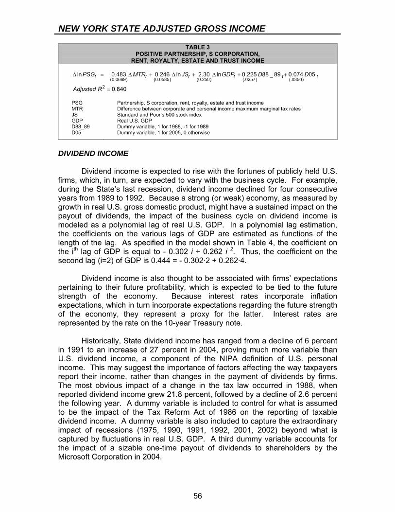
NEW YORK STATE ADJUSTED GROSS INCOME
56
TABLE 3 POSITIVE PARTNERSHIP, S CORPORATION,
RENT, ROYALTY, ESTATE AND TRUST INCOME
(0.0669) (0.0585) (0.250) (.0257) (.0350)2
ln 0.483 0.246 ln 2.30 ln 0.225 88 _ 89 0.074 05
0.840
t t t t t tPSG MTR JS GDP D D
Adjusted R
Δ = Δ + Δ + Δ + +
= PSG Partnership, S corporation, rent, royalty, estate and trust income MTR Difference between corporate and personal income maximum marginal tax rates JS Standard and Poor’s 500 stock index GDP Real U.S. GDP D88_89 Dummy variable, 1 for 1988, -1 for 1989 D05 Dummy variable, 1 for 2005, 0 otherwise
DIVIDEND INCOME Dividend income is expected to rise with the fortunes of publicly held U.S. firms, which, in turn, are expected to vary with the business cycle. For example, during the State’s last recession, dividend income declined for four consecutive years from 1989 to 1992. Because a strong (or weak) economy, as measured by growth in real U.S. gross domestic product, might have a sustained impact on the payout of dividends, the impact of the business cycle on dividend income is modeled as a polynomial lag of real U.S. GDP. In a polynomial lag estimation, the coefficients on the various lags of GDP are estimated as functions of the length of the lag. As specified in the model shown in Table 4, the coefficient on the ith lag of GDP is equal to - 0.302 i + 0.262 i 2. Thus, the coefficient on the second lag (i=2) of GDP is 0.444 = - 0.302·2 + 0.262·4. Dividend income is also thought to be associated with firms’ expectations pertaining to their future profitability, which is expected to be tied to the future strength of the economy. Because interest rates incorporate inflation expectations, which in turn incorporate expectations regarding the future strength of the economy, they represent a proxy for the latter. Interest rates are represented by the rate on the 10-year Treasury note. Historically, State dividend income has ranged from a decline of 6 percent in 1991 to an increase of 27 percent in 2004, proving much more variable than U.S. dividend income, a component of the NIPA definition of U.S. personal income. This may suggest the importance of factors affecting the way taxpayers report their income, rather than changes in the payment of dividends by firms. The most obvious impact of a change in the tax law occurred in 1988, when reported dividend income grew 21.8 percent, followed by a decline of 2.6 percent the following year. A dummy variable is included to control for what is assumed to be the impact of the Tax Reform Act of 1986 on the reporting of taxable dividend income. A dummy variable is also included to capture the extraordinary impact of recessions (1975, 1990, 1991, 1992, 2001, 2002) beyond what is captured by fluctuations in real U.S. GDP. A third dummy variable accounts for the impact of a sizable one-time payout of dividends to shareholders by the Microsoft Corporation in 2004.
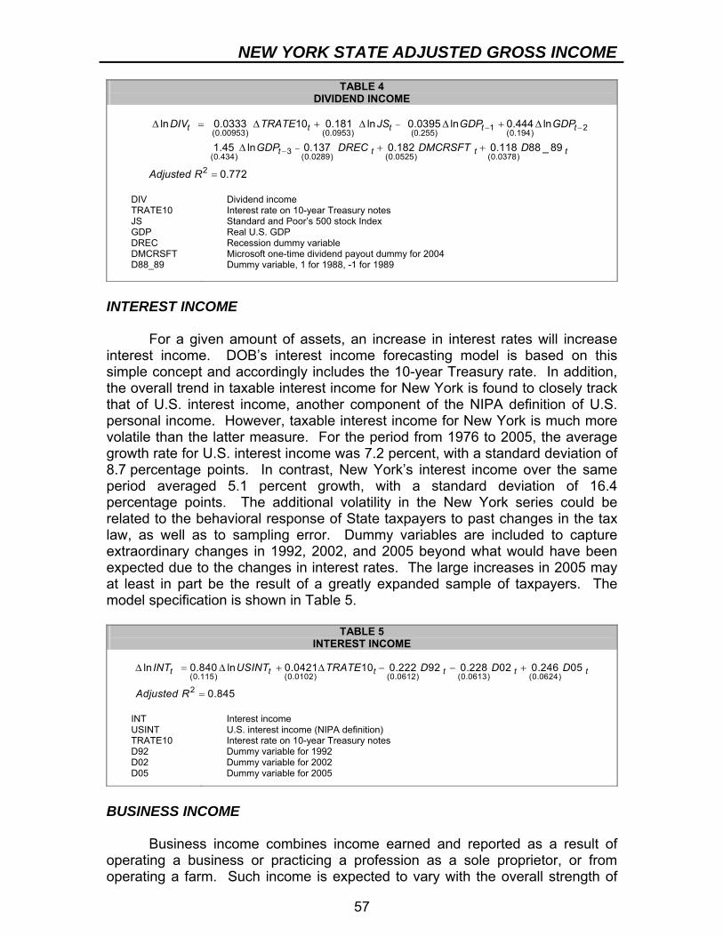
NEW YORK STATE ADJUSTED GROSS INCOME
57
TABLE 4 DIVIDEND INCOME
1 2(0.00953) (0.0953) (0.255) (0.194)
3(0.434) (0.0289) (0.0525) (0.0378)
2
ln 0.0333 10 0.181 ln 0.0395 ln 0.444 ln
1.45 ln 0.137 0.182 0.118 88 _ 89
0.7
t t t t t
t t t t
DIV TRATE JS GDP GDP
GDP DREC DMCRSFT D
Adjusted R
− − −
−−
Δ = Δ + Δ Δ + Δ
Δ + +
= 72
DIV Dividend income TRATE10 Interest rate on 10-year Treasury notes JS Standard and Poor’s 500 stock Index GDP Real U.S. GDP DREC Recession dummy variable DMCRSFT Microsoft one-time dividend payout dummy for 2004 D88_89 Dummy variable, 1 for 1988, -1 for 1989
INTEREST INCOME For a given amount of assets, an increase in interest rates will increase interest income. DOB’s interest income forecasting model is based on this simple concept and accordingly includes the 10-year Treasury rate. In addition, the overall trend in taxable interest income for New York is found to closely track that of U.S. interest income, another component of the NIPA definition of U.S. personal income. However, taxable interest income for New York is much more volatile than the latter measure. For the period from 1976 to 2005, the average growth rate for U.S. interest income was 7.2 percent, with a standard deviation of 8.7 percentage points. In contrast, New York’s interest income over the same period averaged 5.1 percent growth, with a standard deviation of 16.4 percentage points. The additional volatility in the New York series could be related to the behavioral response of State taxpayers to past changes in the tax law, as well as to sampling error. Dummy variables are included to capture extraordinary changes in 1992, 2002, and 2005 beyond what would have been expected due to the changes in interest rates. The large increases in 2005 may at least in part be the result of a greatly expanded sample of taxpayers. The model specification is shown in Table 5.
TABLE 5 INTEREST INCOME
(0.115) (0.0102) (0.0612) (0.0613) (0.0624)
2
ln 0.840 ln 0.0421 10 0.222 92 0.228 02 0.246 05
0.845
t t t t t tINT USINT TRATE D D D
Adjusted R
Δ = Δ + Δ − − +
=
INT Interest income USINT U.S. interest income (NIPA definition) TRATE10 Interest rate on 10-year Treasury notes D92 Dummy variable for 1992 D02 Dummy variable for 2002 D05 Dummy variable for 2005
BUSINESS INCOME Business income combines income earned and reported as a result of operating a business or practicing a profession as a sole proprietor, or from operating a farm. Such income is expected to vary with the overall strength of
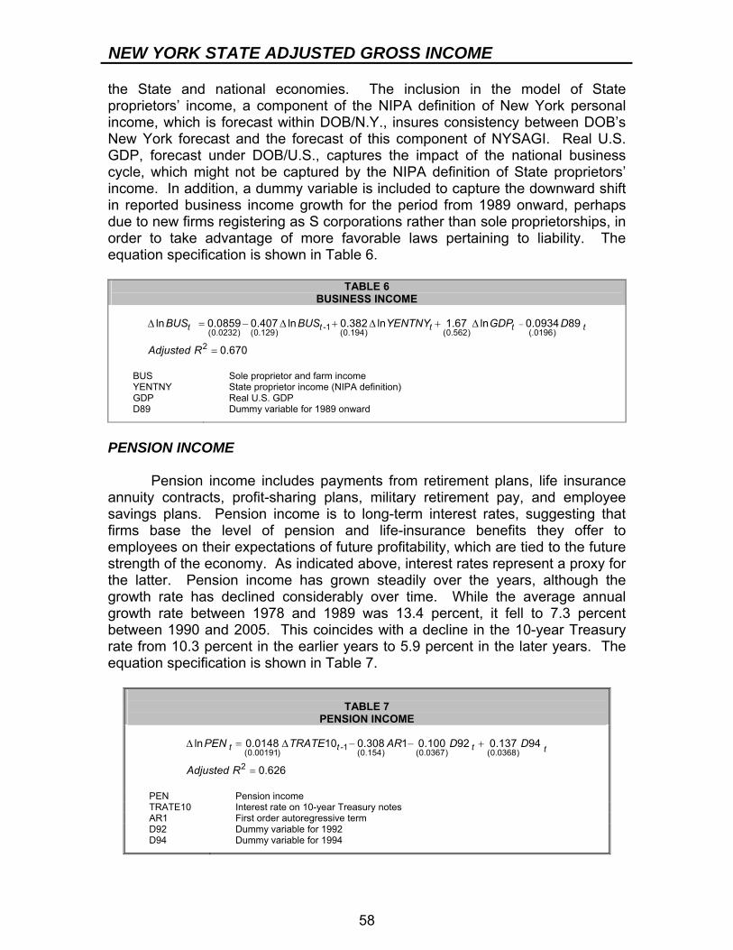
NEW YORK STATE ADJUSTED GROSS INCOME
58
the State and national economies. The inclusion in the model of State proprietors’ income, a component of the NIPA definition of New York personal income, which is forecast within DOB/N.Y., insures consistency between DOB’s New York forecast and the forecast of this component of NYSAGI. Real U.S. GDP, forecast under DOB/U.S., captures the impact of the national business cycle, which might not be captured by the NIPA definition of State proprietors’ income. In addition, a dummy variable is included to capture the downward shift in reported business income growth for the period from 1989 onward, perhaps due to new firms registering as S corporations rather than sole proprietorships, in order to take advantage of more favorable laws pertaining to liability. The equation specification is shown in Table 6.
TABLE 6 BUSINESS INCOME
-1(0.0232) (0.129) (0.194) (0.562) (.0196)2
ln 0.0859 0.407 ln 0.382 ln 1.67 ln 0.0934 89
0.670
t t t t tBUS BUS YENTNY GDP D
Adjusted R
−Δ = − Δ + Δ + Δ
=
BUS Sole proprietor and farm income YENTNY State proprietor income (NIPA definition) GDP Real U.S. GDP D89 Dummy variable for 1989 onward
PENSION INCOME Pension income includes payments from retirement plans, life insurance annuity contracts, profit-sharing plans, military retirement pay, and employee savings plans. Pension income is to long-term interest rates, suggesting that firms base the level of pension and life-insurance benefits they offer to employees on their expectations of future profitability, which are tied to the future strength of the economy. As indicated above, interest rates represent a proxy for the latter. Pension income has grown steadily over the years, although the growth rate has declined considerably over time. While the average annual growth rate between 1978 and 1989 was 13.4 percent, it fell to 7.3 percent between 1990 and 2005. This coincides with a decline in the 10-year Treasury rate from 10.3 percent in the earlier years to 5.9 percent in the later years. The equation specification is shown in Table 7.
TABLE 7
PENSION INCOME
-1(0.00191) (0.154) (0.0367) (0.0368)2
ln 0.0148 10 0.308 1 0.100 92 0.137 94
0.626
t t t tPEN TRATE AR D D
Adjusted R
Δ = Δ − − +
=
PEN Pension income TRATE10 Interest rate on 10-year Treasury notes AR1 First order autoregressive term D92 Dummy variable for 1992 D94 Dummy variable for 1994
NEW YORK STATE ADJUSTED GROSS INCOME
59
RISK ASSESSMENT AND FAN CHARTS Introduction The Division of the Budget uses forecasting models to project future values for the components of New York State adjusted gross income (NYSAGI). By and large, these models presume that the historical relationships between the components of income and a number of key economic indicators are useful for projecting their future behavior, and that these relationships are stable and can be estimated using standard statistical methods. Since all statistical models are simplifications of complex relationships, they are subject to model misspecification error. In addition, there are risks associated with the forecasts for the exogenous economic indicators. Even if a model is well specified and the future values of the exogenous inputs can be predicted with certainty, a statistical forecast remains subject to error. There is always a component that cannot be captured by the model, which is simply ascribed to random variation. And the estimated parameters of the model are themselves random variables and, as such, subject to estimation error. The tool used by the Division of the Budget for presenting the risk to the forecast is the fan chart. Fan charts display prediction intervals as shown in the sample chart below (see Figure 1). It is estimated that with 90 percent probability, future values will fall into the shaded area of the fan. Each band within the shaded area reflects five percent probability regions. The chart "fans out" over time to reflect the increasing uncertainty and growing risk as the forecast departs further from the base year. Not only does the fan chart graphically depict the risks associated with a point forecast as time progresses, but it also highlights how realizations that are quite far from the point estimate can have a reasonably high likelihood of occurring. Fan charts can exhibit skewness that reflects more downside or upside risk to the forecast, and the costs associated with erring on either side.
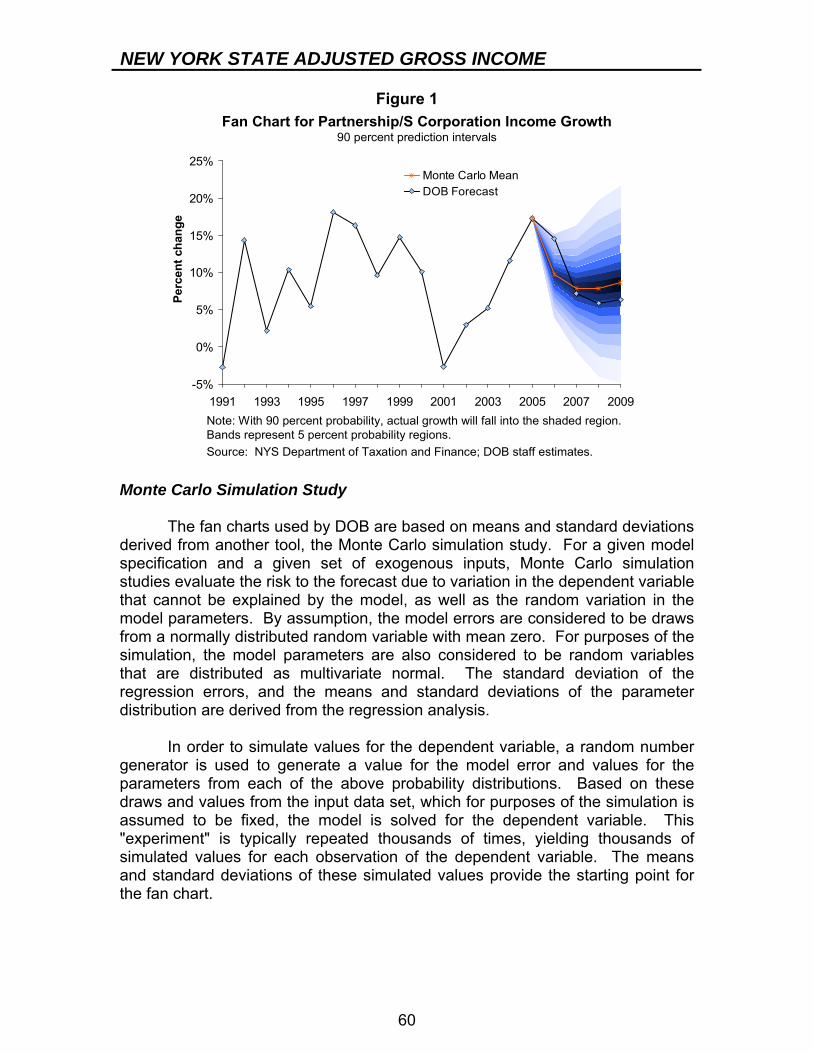
NEW YORK STATE ADJUSTED GROSS INCOME
60
Figure 1
-5%
0%
5%
10%
15%
20%
25%
1991 1993 1995 1997 1999 2001 2003 2005 2007 2009
Monte Carlo MeanDOB Forecast
Perc
ent c
hang
e
Fan Chart for Partnership/S Corporation Income Growth90 percent prediction intervals
Note: With 90 percent probability, actual growth will fall into the shaded region. Bands represent 5 percent probability regions. Source: NYS Department of Taxation and Finance; DOB staff estimates.
Monte Carlo Simulation Study The fan charts used by DOB are based on means and standard deviations derived from another tool, the Monte Carlo simulation study. For a given model specification and a given set of exogenous inputs, Monte Carlo simulation studies evaluate the risk to the forecast due to variation in the dependent variable that cannot be explained by the model, as well as the random variation in the model parameters. By assumption, the model errors are considered to be draws from a normally distributed random variable with mean zero. For purposes of the simulation, the model parameters are also considered to be random variables that are distributed as multivariate normal. The standard deviation of the regression errors, and the means and standard deviations of the parameter distribution are derived from the regression analysis. In order to simulate values for the dependent variable, a random number generator is used to generate a value for the model error and values for the parameters from each of the above probability distributions. Based on these draws and values from the input data set, which for purposes of the simulation is assumed to be fixed, the model is solved for the dependent variable. This "experiment" is typically repeated thousands of times, yielding thousands of simulated values for each observation of the dependent variable. The means and standard deviations of these simulated values provide the starting point for the fan chart.
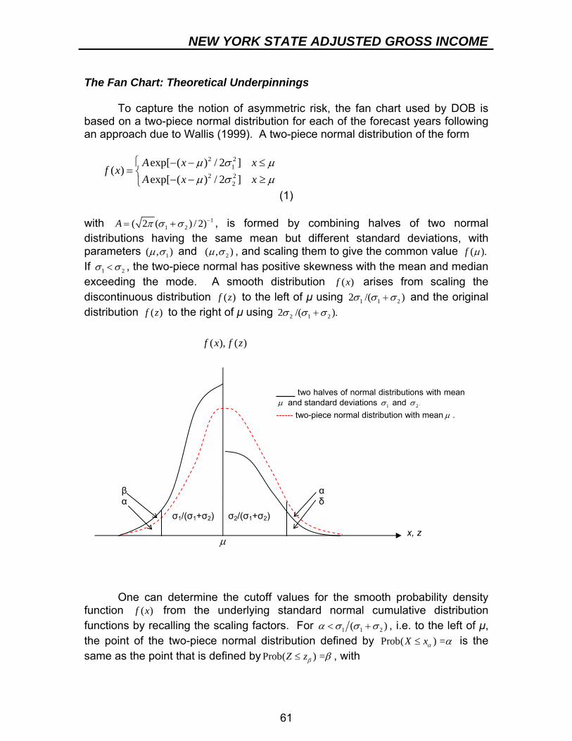
NEW YORK STATE ADJUSTED GROSS INCOME
61
The Fan Chart: Theoretical Underpinnings To capture the notion of asymmetric risk, the fan chart used by DOB is based on a two-piece normal distribution for each of the forecast years following an approach due to Wallis (1999). A two-piece normal distribution of the form
2 21
2 22
exp[ ( ) / 2 ]( )
exp[ ( ) / 2 ]A x x
f xA x x
μ σ μμ σ μ
⎧ − − ≤= ⎨
− − ≥⎩ (1)
with 1
1 2( 2 ( ) / 2)π σ σ −= +A , is formed by combining halves of two normal distributions having the same mean but different standard deviations, with parameters 1( , )μ σ and 2( , )μ σ , and scaling them to give the common value ( ).f μ If 1 2σ σ< , the two-piece normal has positive skewness with the mean and median exceeding the mode. A smooth distribution ( )f x arises from scaling the discontinuous distribution ( )f z to the left of μ using 1 1 22 /( )σ σ σ+ and the original distribution ( )f z to the right of μ using 2 1 22 /( ).σ σ σ+
One can determine the cutoff values for the smooth probability density function ( )f x from the underlying standard normal cumulative distribution functions by recalling the scaling factors. For 1 1 2( )α σ σ σ< + , i.e. to the left of μ, the point of the two-piece normal distribution defined by Prob( ) =X xα α≤ is the same as the point that is defined by Prob( ) =≤Z zβ β , with
μ
β α
α δ
σ1/(σ1+σ2) σ2/(σ1+σ2)
x, z
( ), ( )f x f z
____ two halves of normal distributions with mean μ and standard deviations 1σ and .2σ ------ two-piece normal distribution with mean μ .
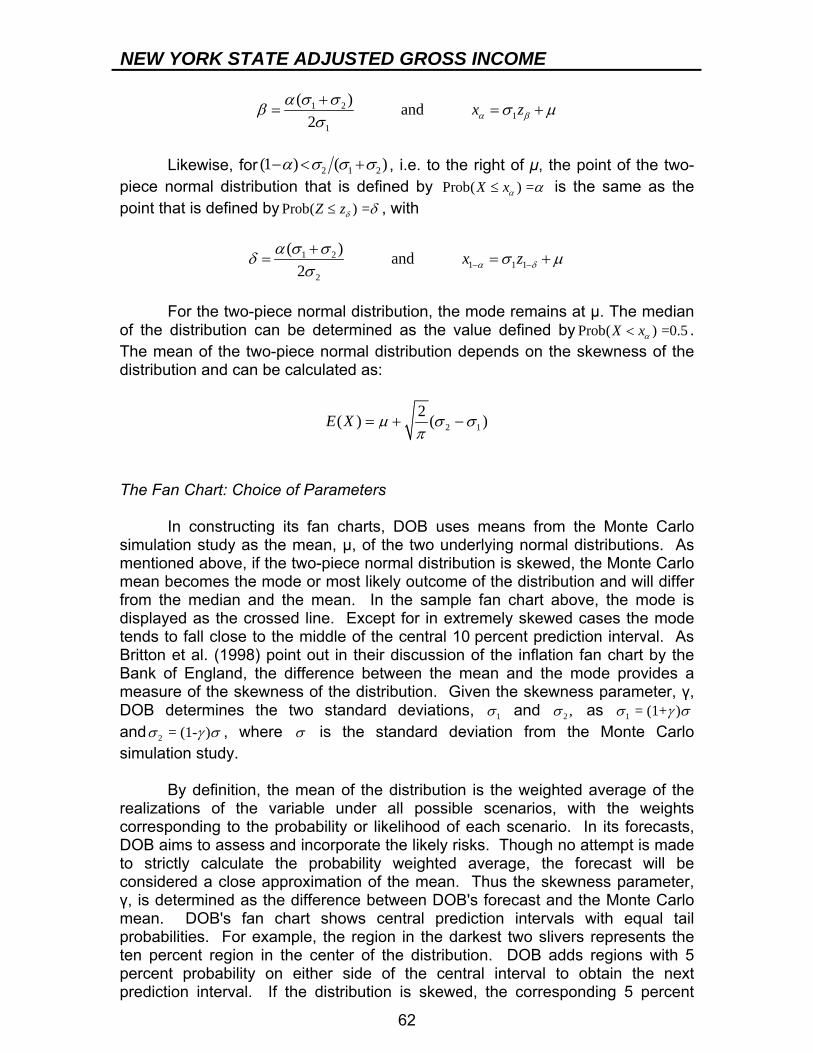
NEW YORK STATE ADJUSTED GROSS INCOME
62
1 21
1
( ) and2
x zα βα σ σβ σ μ
σ+
= = +
Likewise, for 2 1 2(1 ) ( )α σ σ σ− < + , i.e. to the right of μ, the point of the two-piece normal distribution that is defined by Prob( ) =X xα α≤ is the same as the point that is defined by Prob( ) =≤Z zδ δ , with
1 21 1 1
2
( ) and2
x zα δα σ σδ σ μ
σ − −
+= = +
For the two-piece normal distribution, the mode remains at μ. The median of the distribution can be determined as the value defined by Prob( ) =0.5<X xα . The mean of the two-piece normal distribution depends on the skewness of the distribution and can be calculated as:
2 12( ) ( )E X μ σ σπ
= + −
The Fan Chart: Choice of Parameters In constructing its fan charts, DOB uses means from the Monte Carlo simulation study as the mean, μ, of the two underlying normal distributions. As mentioned above, if the two-piece normal distribution is skewed, the Monte Carlo mean becomes the mode or most likely outcome of the distribution and will differ from the median and the mean. In the sample fan chart above, the mode is displayed as the crossed line. Except for in extremely skewed cases the mode tends to fall close to the middle of the central 10 percent prediction interval. As Britton et al. (1998) point out in their discussion of the inflation fan chart by the Bank of England, the difference between the mean and the mode provides a measure of the skewness of the distribution. Given the skewness parameter, γ, DOB determines the two standard deviations, 1σ and 2 ,σ as 1 = (1+ )σ γ σ and 2 = (1- )σ γ σ , where σ is the standard deviation from the Monte Carlo simulation study. By definition, the mean of the distribution is the weighted average of the realizations of the variable under all possible scenarios, with the weights corresponding to the probability or likelihood of each scenario. In its forecasts, DOB aims to assess and incorporate the likely risks. Though no attempt is made to strictly calculate the probability weighted average, the forecast will be considered a close approximation of the mean. Thus the skewness parameter, γ, is determined as the difference between DOB's forecast and the Monte Carlo mean. DOB's fan chart shows central prediction intervals with equal tail probabilities. For example, the region in the darkest two slivers represents the ten percent region in the center of the distribution. DOB adds regions with 5 percent probability on either side of the central interval to obtain the next prediction interval. If the distribution is skewed, the corresponding 5 percent
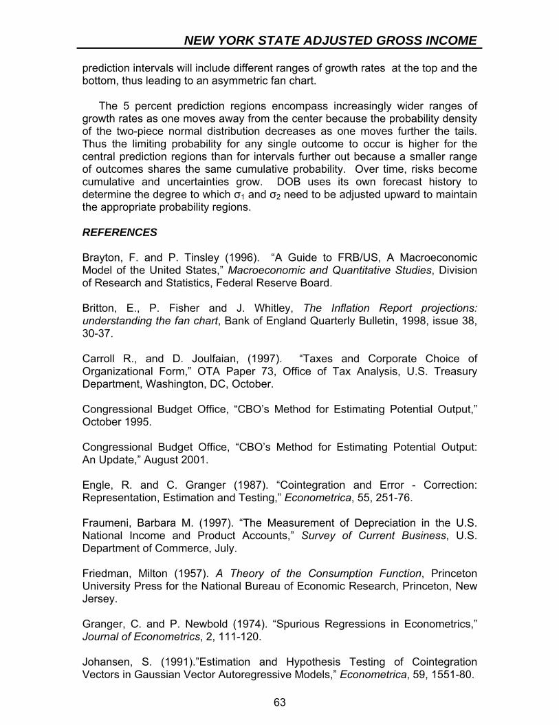
NEW YORK STATE ADJUSTED GROSS INCOME
63
prediction intervals will include different ranges of growth rates at the top and the bottom, thus leading to an asymmetric fan chart.
The 5 percent prediction regions encompass increasingly wider ranges of
growth rates as one moves away from the center because the probability density of the two-piece normal distribution decreases as one moves further the tails. Thus the limiting probability for any single outcome to occur is higher for the central prediction regions than for intervals further out because a smaller range of outcomes shares the same cumulative probability. Over time, risks become cumulative and uncertainties grow. DOB uses its own forecast history to determine the degree to which σ1 and σ2 need to be adjusted upward to maintain the appropriate probability regions. REFERENCES Brayton, F. and P. Tinsley (1996). “A Guide to FRB/US, A Macroeconomic Model of the United States,” Macroeconomic and Quantitative Studies, Division of Research and Statistics, Federal Reserve Board. Britton, E., P. Fisher and J. Whitley, The Inflation Report projections: understanding the fan chart, Bank of England Quarterly Bulletin, 1998, issue 38, 30-37. Carroll R., and D. Joulfaian, (1997). “Taxes and Corporate Choice of Organizational Form,” OTA Paper 73, Office of Tax Analysis, U.S. Treasury Department, Washington, DC, October. Congressional Budget Office, “CBO’s Method for Estimating Potential Output,” October 1995. Congressional Budget Office, “CBO’s Method for Estimating Potential Output: An Update,” August 2001. Engle, R. and C. Granger (1987). “Cointegration and Error - Correction: Representation, Estimation and Testing,” Econometrica, 55, 251-76. Fraumeni, Barbara M. (1997). “The Measurement of Depreciation in the U.S. National Income and Product Accounts,” Survey of Current Business, U.S. Department of Commerce, July. Friedman, Milton (1957). A Theory of the Consumption Function, Princeton University Press for the National Bureau of Economic Research, Princeton, New Jersey. Granger, C. and P. Newbold (1974). “Spurious Regressions in Econometrics,” Journal of Econometrics, 2, 111-120. Johansen, S. (1991).”Estimation and Hypothesis Testing of Cointegration Vectors in Gaussian Vector Autoregressive Models,” Econometrica, 59, 1551-80.
NEW YORK STATE ADJUSTED GROSS INCOME
64
Lucas, Robert E. (1976). “Econometric Policy Evaluation: A Critique,” The Phillips Curve and Labor Markets, Carnegie Rochester Series on Public Policy, Vol. 1, edited by Brunner, K. and Meltzer, A. H., 19-46. Miller, Preston and Larry Ozanne (2000). “Forecasting Capital Gains Realizations,” Congressional Budget Office, August. Nelson, C. R. and C. I. Plosser (1982). “Trends and Random Walks in Macroeconomic Time Series,” Journal of Monetary Economics, 10, 139-162, 1982. Orphanides, Athanasios (2003). “Historical Monetary Policy Analysis and the Taylor Rule,” The Federal Reserve Board, Finance and Economic Discussion Series 2003-36 (June). Phillips, P. C. B. (1991). “Optimal Inference in Cointegrated Systems,” Econometrica, 59, 283-306. Rudd, Jeremy and Karl Whelan (2003). “Can Rational Expectations Sticky-Price Models Explain Inflation Dynamics?” The Federal Reserve Board, Finance and Economic Discussion Series 2003-46 (September). Roberts, John M. (2001). “How Well Does the New Keynesian Sticky-Price Model Fit the Data?” The Federal Reserve Board, Finance and Economic Discussion Series 2001-13 (February). Sims, Christopher A. (2003). “Implications of Rational Inattention,” Journal of Monetary Economics, 50, 665-690. Sims, Christopher A. (1980). “Macroeconomics and Reality,” Econometrica, 48, 1-48. Taylor, John B. (1993). “Discretion Versus Policy Rules in Practice,” Carnegie-Rochester Conference Series on Public Policy, 39, 195-214. Tevlin, S. and Karl Whelan (2003). “Explaining the Investment Boom of the 1990s,” Journal of Money, Credit, and Banking, 35 (February), 1-22. Wallis, K.F. (1999). Asymmetric Density Forecasts of Inflation and the Bank of England's Fan Chart, National Institute Economic Review, January, 106-112. Woodford, Michael (2002). “Interest and Price — Foundations of a Theory of Monetary Policy,” Princeton University Press.
Part II - Revenue Methodologies

67
PERSONAL INCOME TAX BACKGROUND Historical The New York State (NYS) personal income tax was originally enacted in 1919, six years after the ratification of the 16th Amendment to the U.S. Constitution allowed the Federal government to levy a personal income tax. A top rate of three percent was imposed on taxable incomes above $50,000 and remained in force until 1930. The present system of conformity with the Federal definition of adjusted gross income and allowing itemized deductions began in 1960. The tax rate schedule shifted several times during the 1970s, with the top rate peaking at 15.375 percent on taxable incomes above $25,000. Since then, the State has undergone several major tax law reforms and reductions, culminating in a top tax rate of 6.85 percent and the implementation of numerous deductions and credits. In May 2003, two new top brackets were added temporarily for the 2003-2005 tax years, having a maximum rate of 7.7 percent. The State’s tax rate schedule returned to 2002 law effective in 2006. The Nature of the Forecasting Problem Detailed knowledge of the composition and distribution of taxable income is critical to accurately projecting future personal income tax (PIT) receipts. Consequently, the PIT forecasting process presents unique challenges. One complicating factor is the complex linkage between economic activity and PIT revenue. Individual taxpayer activities generate various forms of taxable income — such as wages, non-corporate business income, capital gains realizations, dividends, and interest income — that give rise to tax liability and, in turn, “cash” payments to the State. There can be long lags between the point in time when the liability is incurred and the cash payment is actually received by the New York State Department of Taxation and Finance. This lag is minimal for wages and salaries due to the withholding mechanism. However, for the non-wage components, such as capital gains realizations and business income, the lag can exceed one year. A related challenge arises from the delay in the availability of liability data, of which the primary source is individual tax returns. The NYS Department of Taxation and Finance provides very timely information on the flow of PIT receipts throughout the tax year. Indeed, withholding data, which tracks wages and salaries closely, are compiled daily, while estimated payments are paid and compiled quarterly throughout the tax year. However, there is no detailed information on the income components that generated the underlying tax liability until tax returns are processed during the following year. The delay is compounded by the ability of taxpayers to request extensions for filing their returns, a common practice among high-income taxpayers. Thus, a solid estimate of 2006 tax liability will not become available until the end of 2007. This estimate will be further refined over the course of the first half of 2008 as Department of Taxation and Finance staff closely inspect and verify a sample of
PERSONAL INCOME TAX
68
tax returns. This sample dataset, known as the personal income tax study file, is expected to become available during the summer of 2008. Detailed information on both the components of taxable income and their distribution is also necessary for analyzing the impact of proposed tax law changes on PIT liability. Tax law changes that affect particular income components may have variable effects on taxpayers depending on their level of incomes. For example, a change in the tax treatment of capital gains would tend to affect higher-income taxpayers more then lower-income taxpayers, all things being equal. Therefore, it is essential to be able to project not only the total value of the components of taxable income, but also how those components are distributed across taxpayers by income. Computing Personal Income Tax Liability The computation of the personal income tax starts with the addition of the taxable components of income to arrive at Federal gross income.1 The Internal Revenue Code permits certain exclusions and adjustments in arriving at Federal adjusted gross income (FAGI). The State requires certain additions and subtractions to FAGI in order to obtain New York State adjusted gross income (NYSAGI). NYSAGI is reduced by the larger of the State standard deduction or the total of itemized deductions. State itemized deductions generally conform to the Federal concept but with certain modifications, such as the add-back of State and local income taxes. New York conforms to Federal law by limiting itemized deductions for taxpayers with FAGI above $159,950 in tax year 2008. Upper-income taxpayers are subject to a further deduction limitation under State law. State taxpayers may also subtract from NYSAGI a $1,000 exemption for each dependent, not including the taxpayer and spouse, in determining taxable income. A graduated tax rate schedule is applied to taxable income to compute the tax owed. In addition, those with NYSAGI above $100,000 must calculate a supplemental tax that “recaptures” the benefit of the lower brackets. Taxpayers arrive at their final tax liability after subtracting whatever credits they may qualify for.2 Taxpayers who qualify for refundable credits, such as the Earned Income Tax Credit and Empire State Child Credit, may even owe “negative” liability, entitling them to a payment from the State. DATA SOURCES Data on the personal income tax (PIT) come primarily from the NYS Department of Taxation and Finance, although ancillary data are obtained from
1 The income components include: wages, salaries and tips; interest and dividend incomes; State and local income tax refunds; alimony received; net business and farm incomes; capital gains and losses; IRA distributions and pensions and annuities; rents and royalties; incomes from partnerships, S corporations and trusts; unemployment compensation; and taxable Social Security benefits. 2 Current State law allows the following major credits: Earned Income Tax Credit; Empire State Child Credit, household credit; child and dependent care credit; real property tax circuit breaker credit; agricultural property tax credit; long-term care insurance credit; college tuition credit; nursing home assessment credit, investment credit; and Empire Zone credits.
PERSONAL INCOME TAX
69
the U.S. Internal Revenue Service (IRS). Detailed descriptions of these various data sources appear below. PIT Study Files PIT study files are created every year by the NYS Department of Taxation and Finance specifically for the purpose of analysis and research. The study file is a statistical sample of income tax returns stratified by region; income; filer type; resident status; whether the taxpayer itemizes deductions or claims the standard deduction; and whether the taxpayer claims one or more business credits, one or more personal credits, or no credits. The most recent study file pertains to the 2005 tax year and contains approximately 620,000 records, representing a substantial increase from prior years. The study file contains detailed information, including: marital and resident status, components of income, Federal and NYS adjusted gross incomes, either the standard deduction or the components of itemized deductions, the number and amount of exemptions, tax liability, and credits. Since the study files contain only a sample of the taxpayer universe, each record has a weight assigned to it such that when file components are multiplied by the weights, the results can be assumed to represent a statistically accurate portrait of the actual New York State taxpayer profile. Processing Reports The Department of Taxation and Finance generates daily, weekly, and monthly collection reports on withholding, estimated payments, and those components of collections that are related to taxpayers’ final settlement with the State for the previous tax year, i.e., their tax returns. The Division of the Budget monitors these data closely for the purposes of both forecasting and performing monthly cash flow analysis. Each component of receipts follows a different payment and reporting schedule. Withholding information is reported on a daily basis,3 while estimated payments follow a quarterly schedule (April-June-September-January). Final payments from taxpayers whose returns are accompanied by a remittance to the State tend to arrive during the March-April-May period, as well as during October when returns are due for taxpayers receiving extensions.4 Refunds on timely filed returns must be issued within 45 days of the due date or within 45 days of the filing date, whichever is later. As a result, most refunds on timely filed returns are paid during the March-April-May period. Tax return processing reports provide year-to-date data on the number of returns filed, tax liability, and NYSAGI well before the study file for the same tax
3 If an employer was required to remit $15,000 or more of withholding tax during the calendar year preceding the previous year, the employer must remit the tax on or before the third business day following the payroll date. If an employer was required to remit less than $15,000, the employer has up to five business days following the date of payroll to send payment for the withholding tax. Employers who are qualified educational organizations or health care providers must remit the tax on or before the fifth business day following the date of payment. Employers who have withheld, but not remitted, a cumulative aggregate amount of less than $700 at the close of a calendar quarter must remit the tax quarterly. 4 Prior to the current year, August 15 was filing deadline for extensions.
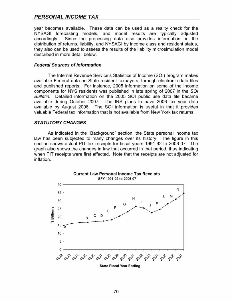
PERSONAL INCOME TAX
70
year becomes available. These data can be used as a reality check for the NYSAGI forecasting models, and model results are typically adjusted accordingly. Since the processing data also provides information on the distribution of returns, liability, and NYSAGI by income class and resident status, they also can be used to assess the results of the liability microsimulation model described in more detail below. Federal Sources of Information The Internal Revenue Service’s Statistics of Income (SOI) program makes available Federal data on State resident taxpayers, through electronic data files and published reports. For instance, 2005 information on some of the income components for NYS residents was published in late spring of 2007 in the SOI Bulletin. Detailed information on the 2005 SOI public use data file became available during October 2007. The IRS plans to have 2006 tax year data available by August 2008. The SOI information is useful in that it provides valuable Federal tax information that is not available from New York tax returns. STATUTORY CHANGES As indicated in the “Background” section, the State personal income tax law has been subjected to many changes over its history. The figure in this section shows actual PIT tax receipts for fiscal years 1991-92 to 2006-07. The graph also shows the changes in law that occurred in that period, thus indicating when PIT receipts were first affected. Note that the receipts are not adjusted for inflation.
Current Law Personal Income Tax Receipts SFY 1991-92 to 2006-07
0
5
10
15
20
25
30
35
40
1992
1993
1994
1995
1996
1997
1998
1999
2000
2001
2002
2003
2004
2005
2006
2007
State Fiscal Year Ending
$ B
illio
ns E
A
D
IH
GF
JK
L
BC
N
M
PERSONAL INCOME TAX
71
A. 1991-92: Changed rate schedule for taxpayers with taxable wages in excess of $90,000 annually to account for the Federal limitation on itemized deductions and for the State tax table benefit recapture.
B. 1994-95: Reflects the enactment of the State earned income tax credit (EITC) at 7.5 percent of the Federal credit, effective for the 1994 tax year.
C. 1995-96: Reflects these changes for the 1995 tax year: standard deduction increased to $6,600 for single individuals, $10,800 for married couples; maximum rate lowered to 7.59 percent and number of tax brackets reduced; EITC increased to 10 percent of the Federal credit.
D. 1996-97: Reflects these changes for 1996 tax year: standard deduction increased to $7,400 for single individuals, $12,350 for married couples; maximum rate lowered to 7 percent while the wage brackets to which the rates apply were broadened; EITC increased to 20 percent of the Federal credit, income levels for the Child and Dependent Care Credit increased and the credit was made refundable.
E. 1997-98: Reflects creation of the Agricultural Property Tax Credit for the 1997 tax year. In addition, reflects these changes for the 1997 tax year: standard deduction raised to $7,500 for single individuals, $13,000 for married couples; maximum rate reduced to 6.85 percent and broadening of the wage brackets to which the rate is applied.
F. 1998-99: Reflects these changes for the 1998 tax year: increase in the Child and Dependent Care Credit to 100 percent of the Federal credit for taxpayers with AGI up to $17,000 and phased down to 20 percent for incomes of $30,000 or more; changed calculation of the Agricultural Property Tax Credit; creation of the Solar Energy Credit; and of the College Choice Tuition Savings Program.
G. 1999-2000: For the Child and Dependent Care Credit, reflects increases in the income levels for the range of the phase down from 100 percent to 20 percent of the Federal credit, setting the range at $35,000 to $50,000 for the 1999 tax year.
H. 2000-01: Reflects these changes for the 2000 tax year: an increase in the Child and Dependent Care Credit raising the maximum to 110 percent of the Federal credit for incomes up to $25,000, with a phase down from 110 percent to 20 percent for incomes above $25,000; an increase in the State EITC to 22.5 percent of the Federal credit; and extension of the Qualified Emerging Technology Credit (QETC) to individuals in partnerships or S corporations.
I. 2001-02: Reflects these changes for the 2001 tax year: another increase in the State EITC to 25 percent of the Federal credit; beginning the first phase of a three-year reduction of the marriage penalty; and providing the first phase of a four-year phase-in of the tuition deduction/credit
J. 2002-03: Reflects these changes for the 2002 tax year: a further increase of the State EITC to 27.5 percent of the Federal credit; providing the second phase of the three-year reduction of the marriage penalty; and the second phase of the four-year phase-in of the tuition deduction/credit.
K. 2003-04: Reflects the following changes: implementation of a three-year temporary surcharge on high-income taxpayers, adopted in 2003, with the second-highest rate falling from 7.5 percent in 2003 to 7.375 percent in
PERSONAL INCOME TAX
72
2004 and to 7.25 percent in 2005 and a top rate of 7.7 percent in all three years; an increase in the State EITC to 30 percent of the Federal credit; provision of the final phase of a three-year reduction of the marriage penalty; and of the third phase of a four-year phase-in of the tuition deduction/credit.
L. 2004-05: Reflects the following changes: continued application of the three-year temporary surcharge; increase in the long-term care insurance credit from 10 to 20 percent; and inclusion of gain from the sale of cooperative housing as NY-source income for nonresidents.
M. 2005-06: Reflects the following changes: continued application of the three-year temporary surcharge, though the final quarter does not include any additional withholding tax because the surcharge expired on 1/1/06; new credit for individual payers of the nursing home assessment.
N. 2006-07: Reflects the following changes: expiration of the temporary personal income tax surcharge reducing the highest tax rate back to 6.85 percent, and the new Empire State Child Credit.
FORECAST METHODOLOGY The estimating/forecasting process for the NYS personal income tax is composed of three major components. They are:
1. The NYS adjusted gross income (NYSAGI) models, comprised of a set of single-equation econometric models that project the individual components of gross taxable income;
2. The PIT microsimulation model, which combines the results from the NYSAGI models with the micro-data from the PIT study file to forecast PIT liability. Microsimulation is also used to assess the impact of tax law changes.
3. The liability-to-cash models, which map calendar-year liability to fiscal-year cash estimates and monitor day-to-day actual cash receipts and refunds.
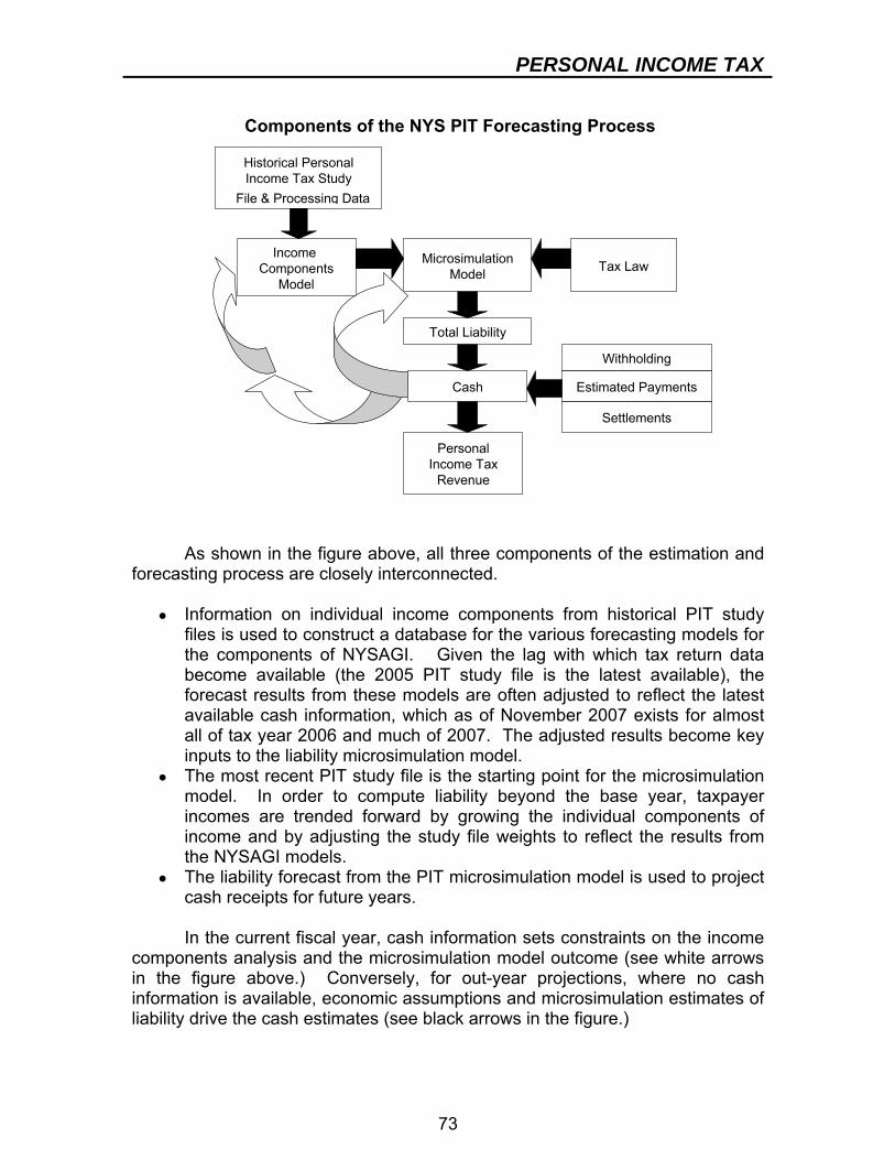
PERSONAL INCOME TAX
73
As shown in the figure above, all three components of the estimation and forecasting process are closely interconnected.
● Information on individual income components from historical PIT study files is used to construct a database for the various forecasting models for the components of NYSAGI. Given the lag with which tax return data become available (the 2005 PIT study file is the latest available), the forecast results from these models are often adjusted to reflect the latest available cash information, which as of November 2007 exists for almost all of tax year 2006 and much of 2007. The adjusted results become key inputs to the liability microsimulation model.
● The most recent PIT study file is the starting point for the microsimulation model. In order to compute liability beyond the base year, taxpayer incomes are trended forward by growing the individual components of income and by adjusting the study file weights to reflect the results from the NYSAGI models.
● The liability forecast from the PIT microsimulation model is used to project cash receipts for future years.
In the current fiscal year, cash information sets constraints on the income components analysis and the microsimulation model outcome (see white arrows in the figure above.) Conversely, for out-year projections, where no cash information is available, economic assumptions and microsimulation estimates of liability drive the cash estimates (see black arrows in the figure.)
Historical Personal Income Tax Study
File & Processing Data
Income Components
Model Microsimulation
Model Tax Law
Total Liability
Cash
PersonalIncome Tax
Revenue
Estimated Payments Withholding
Settlements
Components of the NYS PIT Forecasting Process
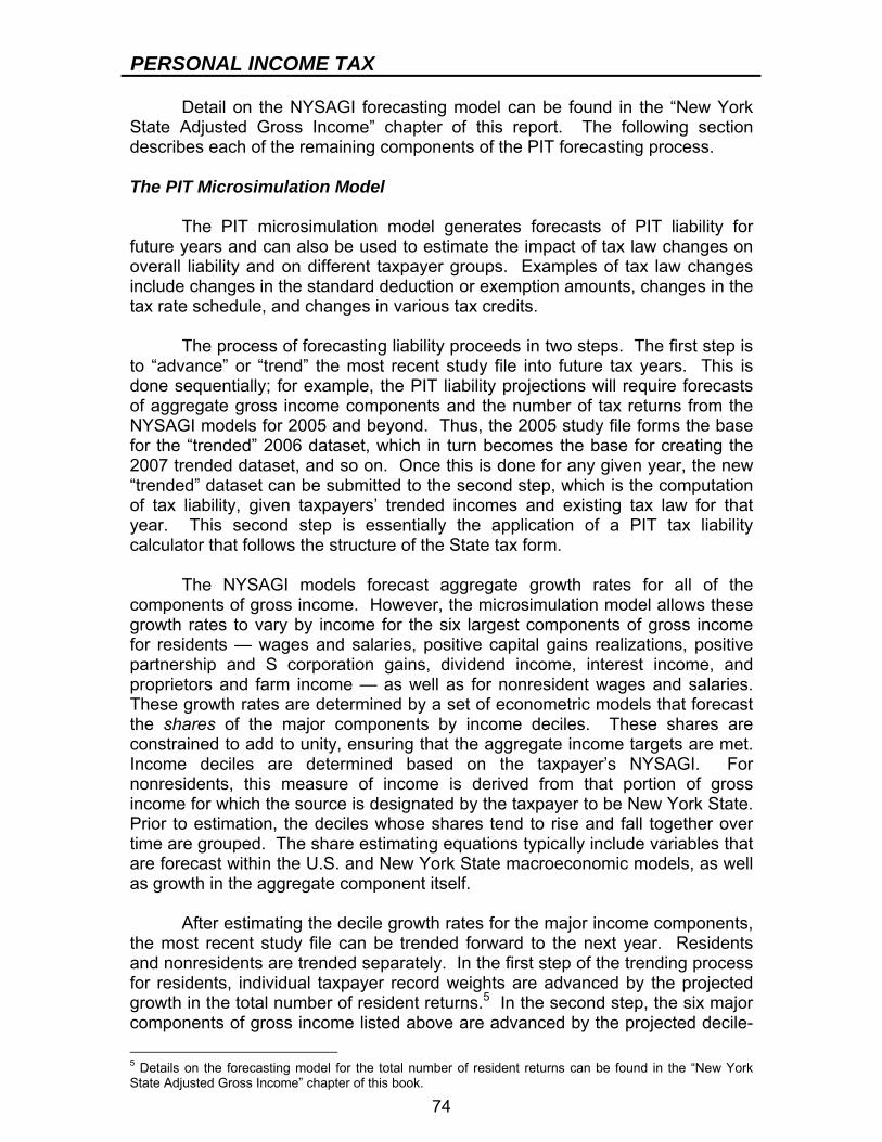
PERSONAL INCOME TAX
74
Detail on the NYSAGI forecasting model can be found in the “New York State Adjusted Gross Income” chapter of this report. The following section describes each of the remaining components of the PIT forecasting process. The PIT Microsimulation Model The PIT microsimulation model generates forecasts of PIT liability for future years and can also be used to estimate the impact of tax law changes on overall liability and on different taxpayer groups. Examples of tax law changes include changes in the standard deduction or exemption amounts, changes in the tax rate schedule, and changes in various tax credits. The process of forecasting liability proceeds in two steps. The first step is to “advance” or “trend” the most recent study file into future tax years. This is done sequentially; for example, the PIT liability projections will require forecasts of aggregate gross income components and the number of tax returns from the NYSAGI models for 2005 and beyond. Thus, the 2005 study file forms the base for the “trended” 2006 dataset, which in turn becomes the base for creating the 2007 trended dataset, and so on. Once this is done for any given year, the new “trended” dataset can be submitted to the second step, which is the computation of tax liability, given taxpayers’ trended incomes and existing tax law for that year. This second step is essentially the application of a PIT tax liability calculator that follows the structure of the State tax form. The NYSAGI models forecast aggregate growth rates for all of the components of gross income. However, the microsimulation model allows these growth rates to vary by income for the six largest components of gross income for residents — wages and salaries, positive capital gains realizations, positive partnership and S corporation gains, dividend income, interest income, and proprietors and farm income — as well as for nonresident wages and salaries. These growth rates are determined by a set of econometric models that forecast the shares of the major components by income deciles. These shares are constrained to add to unity, ensuring that the aggregate income targets are met. Income deciles are determined based on the taxpayer’s NYSAGI. For nonresidents, this measure of income is derived from that portion of gross income for which the source is designated by the taxpayer to be New York State. Prior to estimation, the deciles whose shares tend to rise and fall together over time are grouped. The share estimating equations typically include variables that are forecast within the U.S. and New York State macroeconomic models, as well as growth in the aggregate component itself.
After estimating the decile growth rates for the major income components, the most recent study file can be trended forward to the next year. Residents and nonresidents are trended separately. In the first step of the trending process for residents, individual taxpayer record weights are advanced by the projected growth in the total number of resident returns.5 In the second step, the six major components of gross income listed above are advanced by the projected decile- 5 Details on the forecasting model for the total number of resident returns can be found in the “New York State Adjusted Gross Income” chapter of this book.
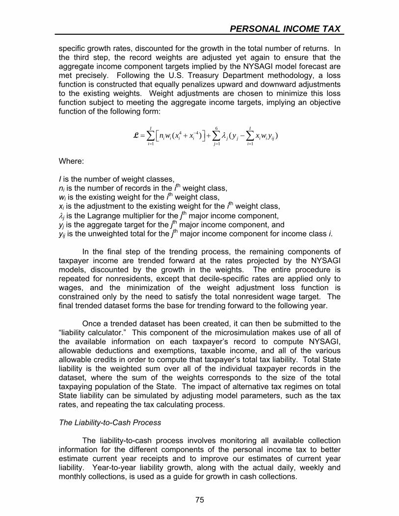
PERSONAL INCOME TAX
75
specific growth rates, discounted for the growth in the total number of returns. In the third step, the record weights are adjusted yet again to ensure that the aggregate income component targets implied by the NYSAGI model forecast are met precisely. Following the U.S. Treasury Department methodology, a loss function is constructed that equally penalizes upward and downward adjustments to the existing weights. Weight adjustments are chosen to minimize this loss function subject to meeting the aggregate income targets, implying an objective function of the following form:
6
4 4
1 1 1( ) ( )
I I
i i i i j j i i iji j i
n w x x y x w yλ−
= = =
⎡ ⎤= + + −⎣ ⎦∑ ∑ ∑L
Where: I is the number of weight classes, ni is the number of records in the ith weight class, wi is the existing weight for the ith weight class, xi is the adjustment to the existing weight for the ith weight class, λj is the Lagrange multiplier for the jth major income component, yj is the aggregate target for the jth major income component, and yij is the unweighted total for the jth major income component for income class i. In the final step of the trending process, the remaining components of taxpayer income are trended forward at the rates projected by the NYSAGI models, discounted by the growth in the weights. The entire procedure is repeated for nonresidents, except that decile-specific rates are applied only to wages, and the minimization of the weight adjustment loss function is constrained only by the need to satisfy the total nonresident wage target. The final trended dataset forms the base for trending forward to the following year. Once a trended dataset has been created, it can then be submitted to the “liability calculator.” This component of the microsimulation makes use of all of the available information on each taxpayer’s record to compute NYSAGI, allowable deductions and exemptions, taxable income, and all of the various allowable credits in order to compute that taxpayer’s total tax liability. Total State liability is the weighted sum over all of the individual taxpayer records in the dataset, where the sum of the weights corresponds to the size of the total taxpaying population of the State. The impact of alternative tax regimes on total State liability can be simulated by adjusting model parameters, such as the tax rates, and repeating the tax calculating process. The Liability-to-Cash Process The liability-to-cash process involves monitoring all available collection information for the different components of the personal income tax to better estimate current year receipts and to improve our estimates of current year liability. Year-to-year liability growth, along with the actual daily, weekly and monthly collections, is used as a guide for growth in cash collections.
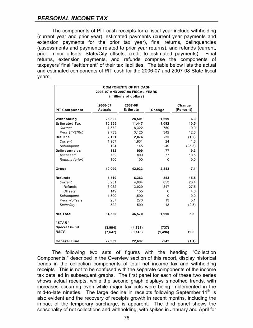
PERSONAL INCOME TAX
76
The components of PIT cash receipts for a fiscal year include withholding (current year and prior year), estimated payments (current year payments and extension payments for the prior tax year), final returns, delinquencies (assessments and payments related to prior year returns), and refunds (current, prior, minor offsets, State/City offsets, credit to estimated payments). Final returns, extension payments, and refunds comprise the components of taxpayers' final "settlement" of their tax liabilities. The table below lists the actual and estimated components of PIT cash for the 2006-07 and 2007-08 State fiscal years.
PIT Com ponent2006-07 Actuals
2007-08 Es tim ate Change
Change (Percent)
Withholding 26,802 28,501 1,699 6.3 Es tim ated Tax 10,355 11,447 1,092 10.5
Current 7,572 8,322 750 9.9 Prior (IT-370s) 2,783 3,125 342 12.3
Re turns 2,101 2,076 -25 (1.2)Current 1,907 1,931 24 1.3 Subsequent 194 145 -49 (25.3)
De linquencies 832 909 77 9.3 Assessed 732 809 77 10.5 Returns (prior) 100 100 0 0.0
Gross 40,090 42,933 2,843 7.1
Re funds 5,510 6,363 853 15.5 Current 3,231 4,084 853 26.4
Refunds 3,082 3,929 847 27.5 Of fsets 149 155 6 4.0
Subsequent 1,500 1,500 0 0.0 Prior w/offsets 257 270 13 5.1 State/City 522 509 -13 (2.5)
1,990 5.8
“STAR” Specia l FundRBTF (7,647) (9,143) (1,496) 19.6
General Fund 22,939 22,697 -242 (1.1)
(737)
Ne t Total 34,580 36,570
(3,994) (4,731)
COM PONENTS OF PIT CASH2006-07 AND 2007-08 FISCAL YEARS
(m illions of dollars )
The following two sets of figures with the heading "Collection Components," described in the Overview section of this report, display historical trends in the collection components of total net income tax and withholding receipts. This is not to be confused with the separate components of the income tax detailed in subsequent graphs. The first panel for each of these two series shows actual receipts, while the second graph displays smoothed trends, with increases occurring even while major tax cuts were being implemented in the mid-to-late nineties. The large decline in receipts following September 11th is also evident and the recovery of receipts growth in recent months, including the impact of the temporary surcharge, is apparent. The third panel shows the seasonality of net collections and withholding, with spikes in January and April for
PERSONAL INCOME TAX
77
total collections, and in January for withholding, particularly noteworthy. The irregular component shows large values relative to trend in recent years, reflecting the stock market boom in the late 1990s and early 2000 and the subsequent recession. The last seven figures show the components of cash liability over time, namely estimated payments, withholding, extensions, and final return payments as a percentage of liability over time, refunds paid as a share of withholding collections, and the major components of PIT cash for the 2005-06 State fiscal year. Note the tendency for the cash components to return to an average percentage of liability. However, the components can deviate significantly from this average in a given year. This tendency to average cash-to-liability ratios forms the basis for the PIT components econometric mode described below.
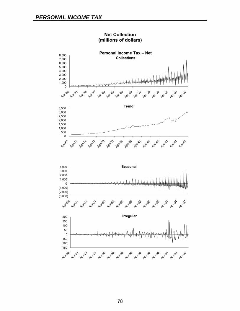
PERSONAL INCOME TAX
78
Net Collection
(millions of dollars)
01,0002,0003,0004,0005,0006,0007,0008,000
Apr-68
Apr-71
Apr-74
Apr-77
Apr-80
Apr-83
Apr-86
Apr-89
Apr-92
Apr-95
Apr-98
Apr-01
Apr-04
Apr-07
Personal Income Tax – NetCollections
0500
1,0001,5002,0002,5003,0003,500
Apr-68
Apr-71
Apr-74
Apr-77
Apr-80
Apr-83
Apr-86
Apr-89
Apr-92
Apr-95
Apr-98
Apr-01
Apr-04
Apr-07
Trend
(3,000)(2,000)(1,000)
01,0002,0003,0004,000
Apr-68
Apr-71
Apr-74
Apr-77
Apr-80
Apr-83
Apr-86
Apr-89
Apr-92
Apr-95
Apr-98
Apr-01
Apr-04
Apr-07
Seasonal
(150)(100)
(50)0
50100150200
Apr-68
Apr-71
Apr-74
Apr-77
Apr-80
Apr-83
Apr-86
Apr-89
Apr-92
Apr-95
Apr-98
Apr-01
Apr-04
Apr-07
Irregular
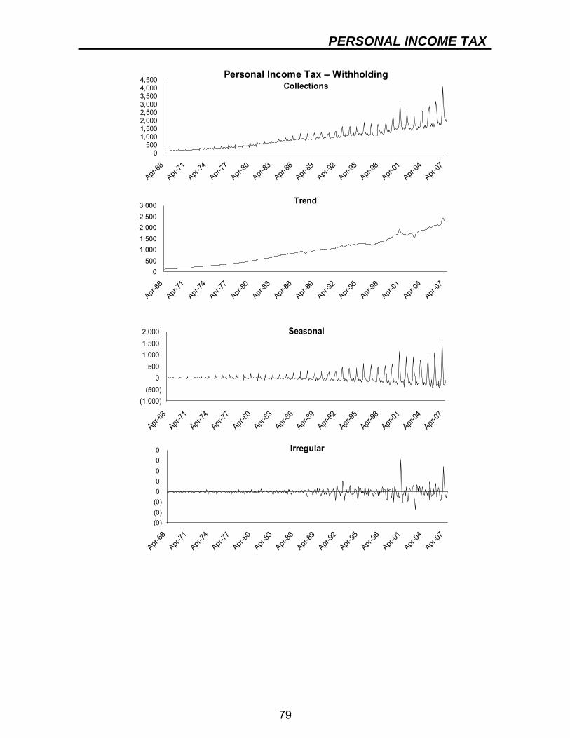
PERSONAL INCOME TAX
79
0500
1,0001,5002,0002,5003,0003,5004,0004,500
Apr-68
Apr-71
Apr-74
Apr-77
Apr-80
Apr-83
Apr-86
Apr-89
Apr-92
Apr-95
Apr-98
Apr-01
Apr-04
Apr-07
Personal Income Tax – WithholdingCollections
0500
1,0001,5002,0002,5003,000
Apr-68
Apr-71
Apr-74
Apr-77
Apr-80
Apr-83
Apr-86
Apr-89
Apr-92
Apr-95
Apr-98
Apr-01
Apr-04
Apr-07
Trend
(1,000)(500)
0500
1,0001,5002,000
Apr-68
Apr-71
Apr-74
Apr-77
Apr-80
Apr-83
Apr-86
Apr-89
Apr-92
Apr-95
Apr-98
Apr-01
Apr-04
Apr-07
Seasonal
(0)(0)(0)00000
Apr-68
Apr-71
Apr-74
Apr-77
Apr-80
Apr-83
Apr-86
Apr-89
Apr-92
Apr-95
Apr-98
Apr-01
Apr-04
Apr-07
Irregular
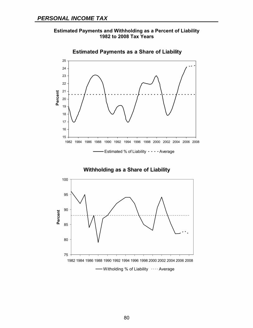
PERSONAL INCOME TAX
80
Estimated Payments and Withholding as a Percent of Liability 1982 to 2008 Tax Years
Estimated Payments as a Share of Liability
15
16
17
18
19
20
21
22
23
24
25
1982 1984 1986 1988 1990 1992 1994 1996 1998 2000 2002 2004 2006 2008
Perc
ent
Estimated % of Liability Average
Withholding as a Share of Liability
75
80
85
90
95
100
1982 1984 1986 1988 1990 1992 1994 1996 1998 2000 2002 2004 2006 2008
Perc
ent
Witholding % of Liability Average
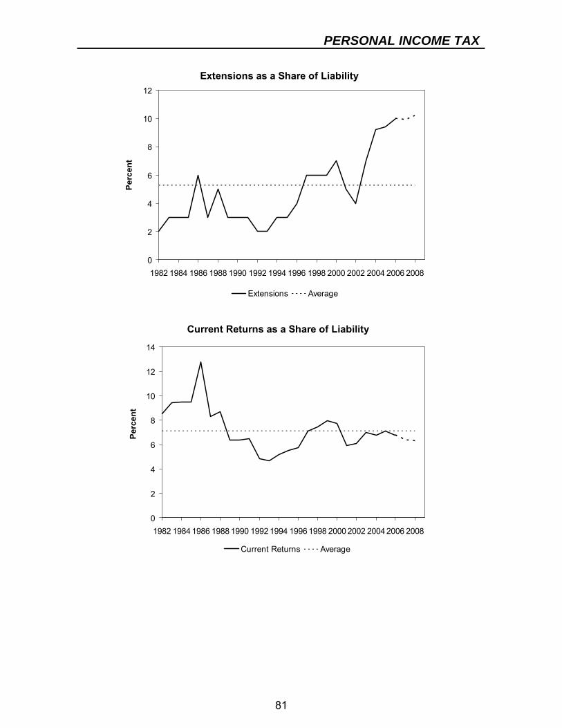
PERSONAL INCOME TAX
81
Extensions as a Share of Liability
0
2
4
6
8
10
12
1982 1984 1986 1988 1990 1992 1994 1996 1998 2000 2002 2004 2006 2008
Extensions Average
Perc
ent
Current Returns as a Share of Liability
0
2
4
6
8
10
12
14
1982 1984 1986 1988 1990 1992 1994 1996 1998 2000 2002 2004 2006 2008
Current Returns Average
Perc
ent
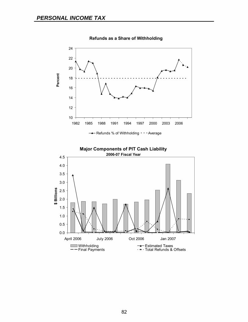
PERSONAL INCOME TAX
82
Refunds as a Share of Withholding
10
12
14
16
18
20
22
24
1982 1985 1988 1991 1994 1997 2000 2003 2006
Refunds % of Withholding Average
Perc
ent
Major Components of PIT Cash Liability 2006-07 Fiscal Year
0.0
0.5
1.0
1.5
2.0
2.5
3.0
3.5
4.0
4.5
April 2006 July 2006 Oct 2006 Jan 2007
$ B
illio
ns
Withholding Estimated TaxesFinal Payments Total Refunds & Offsets
PERSONAL INCOME TAX
83
As discussed earlier, information regarding the various components of tax collections is received on a daily, weekly, and monthly basis. Staff monitors tax collections and other information closely throughout the year to assess the performance of the estimates. For example, as a $26 billion+ component of collections, withholding collections generally are monitored on a daily basis throughout the year, while payments with returns and extension requests as well as refunds are monitored most intensively in April and May of each year. An all-encompassing report on cash collection components of the personal income tax is received from the Department of Taxation and Finance mid-month for the prior month. This report is used to determine the official cash flow for the month. Equipped with this information, staff compares the original estimate for the month, and for the entire fiscal year, with all available actual cash information on each of the components. At the end of each quarter, this information is used, along with historical information and Tax Law changes, to make necessary adjustments to the cash liability estimate. Another critical aspect of the cash-to-liability process is forecasting the different components of receipts on a fiscal-year basis using results from the PIT simulation as a benchmark. Various methodologies are applied for different components of receipts. The largest component of income tax collections, withholding, is estimated based on quarterly forecasts of NYS wages. Withholding is estimated using two alternative methodologies. One method applies a withholding-to-wage growth elasticity to the forecasted growth rates for wages on a quarterly basis to estimate withholding growth rates for each quarter in the forecast period. The elasticity used for each quarter is based on historical elasticity trends and expected future elasticity changes. The second method employs an econometric model to forecast withholding based on independent variables, including wages and shift variables reflecting law changes. More specifically, withholding is a function of quarterly wages, seasonal effects, and dummy variables for Tax Law changes. The wage impact is expected to vary by quarter. This effect is captured by multiplying wages with quarterly dummies. The form of the estimating equation is outlined below. The model takes a simple dynamic form. The fourth lag of the dependent variable (the log of withholding) is included as an explanatory variable. The dynamic element in the model helps to explain the persistence in withholding at seasonal frequencies. The model is estimated in log form. This means we can interpret the coefficients on the wage variables as elasticities. The results are summarized in the following table. The model is estimated using quarterly data starting in 1975 and running through the third quarter of 2007. The summary table shows that the model fit is good and there is no evidence of serial correlation. The elasticity estimates derived from the model are consistent with a priori expectations — we expect withholding to increase (decrease) at a faster rate than wages as people move through the graduated tax brackets. Given that the model is estimated in logs,
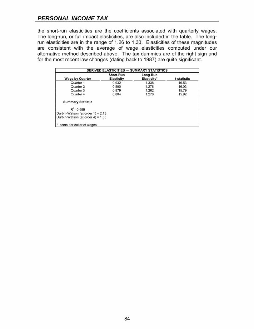
PERSONAL INCOME TAX
84
the short-run elasticities are the coefficients associated with quarterly wages. The long-run, or full impact elasticities, are also included in the table. The long-run elasticities are in the range of 1.26 to 1.33. Elasticities of these magnitudes are consistent with the average of wage elasticities computed under our alternative method described above. The tax dummies are of the right sign and for the most recent law changes (dating back to 1987) are quite significant.
DERIVED ELASTICITIES — SUMMARY STATISTICS
Wage by Quarter Short-Run Elasticity
Long-Run Elasticity*
t-statistic
Quarter 1 0.932 1.338 16.53 Quarter 2 0.890 1.278 16.03 Quarter 3 0.879 1.262 15.79 Quarter 4 0.884 1.270 15.92
Summary Statistic
R2= 0.999
Durbin-Watson (at order 1) = 2.13 Durbin-Watson (at order 4) = 1.65
* cents per dollar of wages
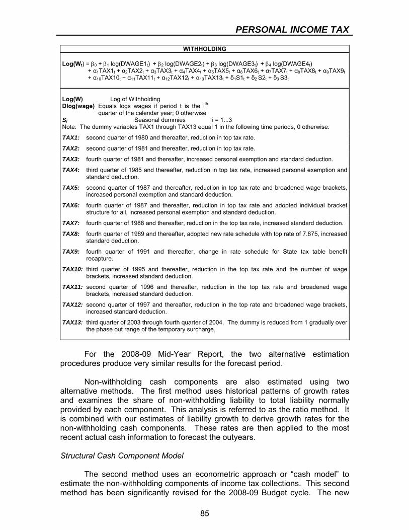
PERSONAL INCOME TAX
85
WITHHOLDING Log(Wt) = β0 + β1 log(DWAGE1t) + β2 log(DWAGE2t) + β3 log(DWAGE3t) + β4 log(DWAGE4t) + α1TAX1t + α2TAX2t + α3TAX3t + α4TAX4t + α5TAX5t + α6TAX6t + α7TAX7t + α8TAX8t + α9TAX9t + α10TAX10t + α11TAX11t + α12TAX12t + α13TAX13t + δ1S1t + δ2 S2t + δ3 S3t Log(W) Log of Withholding Dlog(wage) Equals logs wages if period t is the ith
quarter of the calendar year; 0 otherwise
Si Seasonal dummies i = 1...3 Note: The dummy variables TAX1 through TAX13 equal 1 in the following time periods, 0 otherwise:
TAX1: second quarter of 1980 and thereafter, reduction in top tax rate.
TAX2: second quarter of 1981 and thereafter, reduction in top tax rate.
TAX3: fourth quarter of 1981 and thereafter, increased personal exemption and standard deduction.
TAX4: third quarter of 1985 and thereafter, reduction in top tax rate, increased personal exemption and standard deduction.
TAX5: second quarter of 1987 and thereafter, reduction in top tax rate and broadened wage brackets, increased personal exemption and standard deduction.
TAX6: fourth quarter of 1987 and thereafter, reduction in top tax rate and adopted individual bracket structure for all, increased personal exemption and standard deduction.
TAX7: fourth quarter of 1988 and thereafter, reduction in the top tax rate, increased standard deduction.
TAX8: fourth quarter of 1989 and thereafter, adopted new rate schedule with top rate of 7.875, increased standard deduction.
TAX9: fourth quarter of 1991 and thereafter, change in rate schedule for State tax table benefit recapture.
TAX10: third quarter of 1995 and thereafter, reduction in the top tax rate and the number of wage brackets, increased standard deduction.
TAX11: second quarter of 1996 and thereafter, reduction in the top tax rate and broadened wage brackets, increased standard deduction.
TAX12: second quarter of 1997 and thereafter, reduction in the top rate and broadened wage brackets, increased standard deduction.
TAX13: third quarter of 2003 through fourth quarter of 2004. The dummy is reduced from 1 gradually over the phase out range of the temporary surcharge.
For the 2008-09 Mid-Year Report, the two alternative estimation procedures produce very similar results for the forecast period. Non-withholding cash components are also estimated using two alternative methods. The first method uses historical patterns of growth rates and examines the share of non-withholding liability to total liability normally provided by each component. This analysis is referred to as the ratio method. It is combined with our estimates of liability growth to derive growth rates for the non-withholding cash components. These rates are then applied to the most recent actual cash information to forecast the outyears. Structural Cash Component Model The second method uses an econometric approach or “cash model” to estimate the non-withholding components of income tax collections. This second method has been significantly revised for the 2008-09 Budget cycle. The new
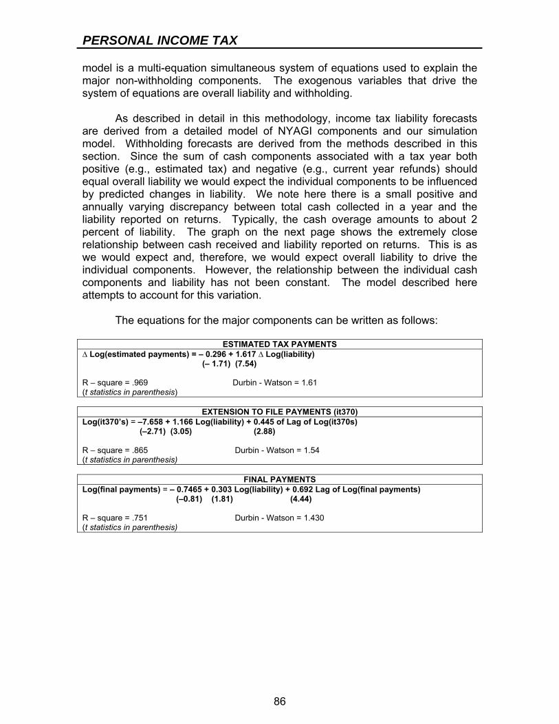
PERSONAL INCOME TAX
86
model is a multi-equation simultaneous system of equations used to explain the major non-withholding components. The exogenous variables that drive the system of equations are overall liability and withholding. As described in detail in this methodology, income tax liability forecasts are derived from a detailed model of NYAGI components and our simulation model. Withholding forecasts are derived from the methods described in this section. Since the sum of cash components associated with a tax year both positive (e.g., estimated tax) and negative (e.g., current year refunds) should equal overall liability we would expect the individual components to be influenced by predicted changes in liability. We note here there is a small positive and annually varying discrepancy between total cash collected in a year and the liability reported on returns. Typically, the cash overage amounts to about 2 percent of liability. The graph on the next page shows the extremely close relationship between cash received and liability reported on returns. This is as we would expect and, therefore, we would expect overall liability to drive the individual components. However, the relationship between the individual cash components and liability has not been constant. The model described here attempts to account for this variation. The equations for the major components can be written as follows:
ESTIMATED TAX PAYMENTS ∆ Log(estimated payments) = – 0.296 + 1.617 ∆ Log(liability)
(– 1.71) (7.54)
R – square = .969 Durbin - Watson = 1.61 (t statistics in parenthesis)
EXTENSION TO FILE PAYMENTS (it370) Log(it370’s) = –7.658 + 1.166 Log(liability) + 0.445 of Lag of Log(it370s)
(–2.71) (3.05) (2.88)
R – square = .865 Durbin - Watson = 1.54 (t statistics in parenthesis)
FINAL PAYMENTS Log(final payments) = – 0.7465 + 0.303 Log(liability) + 0.692 Lag of Log(final payments)
(–0.81) (1.81) (4.44)
R – square = .751 Durbin - Watson = 1.430 (t statistics in parenthesis)
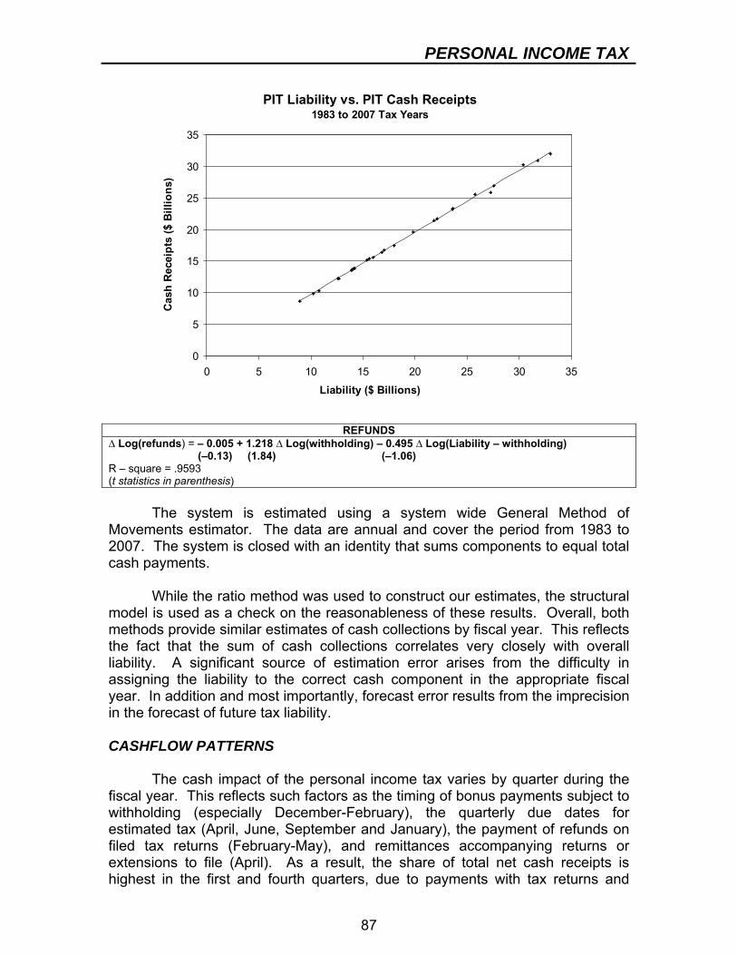
PERSONAL INCOME TAX
87
PIT Liability vs. PIT Cash Receipts 1983 to 2007 Tax Years
0
5
10
15
20
25
30
35
0 5 10 15 20 25 30 35
Liability ($ Billions)
Cas
h R
ecei
pts
($ B
illio
ns)
REFUNDS ∆ Log(refunds) = – 0.005 + 1.218 ∆ Log(withholding) – 0.495 ∆ Log(Liability – withholding)
(–0.13) (1.84) (–1.06) R – square = .9593 (t statistics in parenthesis) The system is estimated using a system wide General Method of Movements estimator. The data are annual and cover the period from 1983 to 2007. The system is closed with an identity that sums components to equal total cash payments. While the ratio method was used to construct our estimates, the structural model is used as a check on the reasonableness of these results. Overall, both methods provide similar estimates of cash collections by fiscal year. This reflects the fact that the sum of cash collections correlates very closely with overall liability. A significant source of estimation error arises from the difficulty in assigning the liability to the correct cash component in the appropriate fiscal year. In addition and most importantly, forecast error results from the imprecision in the forecast of future tax liability. CASHFLOW PATTERNS The cash impact of the personal income tax varies by quarter during the fiscal year. This reflects such factors as the timing of bonus payments subject to withholding (especially December-February), the quarterly due dates for estimated tax (April, June, September and January), the payment of refunds on filed tax returns (February-May), and remittances accompanying returns or extensions to file (April). As a result, the share of total net cash receipts is highest in the first and fourth quarters, due to payments with tax returns and
PERSONAL INCOME TAX
88
bonus withholding/fourth quarter estimated tax installments, respectively. The following table shows net collections by fiscal year quarter in recent years:
PERCENTAGE DISTRIBUTION OF CASH RECEIPTS 1st Quarter 2nd Quarter 3rd Quarter 4th Quarter 1998-99 26.4 22.1 23.1 28.4 1999-2000 25.9 21.2 22.8 30.1 2000-01 26.3 21.0 21.3 31.4 2001-02 30.8 20.4 22.5 26.2 2002-03 25.5 22.9 22.8 28.8 2003-04 21.5 23.1 23.8 31.6 2004-05 24.2 21.8 23.0 31.0 2005-06 26.5 21.8 21.0 30.7 2006-07 28.0 20.8 19.2 32.0 2007-08 (est.) 27.2 21.7 19.6 31.5
RISKS TO THE LIABILITY FORECAST The PIT liability forecast is subject to all of the risks that pertain to the forecast of wages and the other components of taxable income. These risks are particularly pronounced for New York State since a significant portion of taxpayer income is tied to the direction of equity markets, financial services industry profits, and real estate activity, all of which have been shown to be extremely volatile. The predominance of those income components that are tied to these volatile areas of the economy, such as capital gains realizations, bonuses and stock incentive payouts, and the concentration of such income in the hands of a relatively small number of high-income taxpayers pose significant risks to the personal income tax forecast.
89
SALES AND USE TAX BACKGROUND Tax Base and Rate New York State has imposed a general sales and use tax since 1965. It is currently the State’s second largest tax revenue source generating over $11 billion annually. The tax rate has been 4 percent since 1971, although a temporary surcharge to 4.25 percent was imposed from June 1, 2003, to May 31, 2005. Counties and cities within the State are authorized to impose an additional 3 percent sales and use tax, although most have temporary authorizations to impose the tax at a higher rate. New York City and 37 counties currently have a State and local combined rate of more than 8 percent, including the 0.375 percent sales tax imposed in the Metropolitan Commuter Transportation District. The highest maximum combined State and local rate is 9 percent in Oneida County. The tax applies to sales and uses within the State of tangible personal property (unless specifically exempt), certain utility service billings, restaurant meals, hotel and motel occupancy, and specified services and admission charges. Certain exemptions such as food, prescription drugs, residential energy, and college textbooks have been enacted to lessen the regressiveness of the tax. Other items, including machinery and equipment used in production and property purchased for resale, are excluded from tax to avoid tax pyramiding. Administration Persons selling taxable property or services are required to register with the Department of Taxation and Finance as sales tax vendors. Vendors generally are required to remit the tax that they have collected quarterly. However, vendors who record more than $300,000 of taxable sales in any of the immediately preceding four quarters must remit the tax monthly, by the twentieth of the month following the month of collection. Vendors collecting less than $3,000 yearly may elect to file annually, in March. Finally, monthly filers collecting more than $500,000 in tax annually are required to remit the tax by electronic funds transfer (EFT). The collections for the first 22 days of the month must be remitted electronically within three business days after the 22nd day. DATA SOURCES The primary sources of data used in the estimation and forecasting methodology for the sales tax are as follows:
● AM043, Department of Taxation and Finance Monthly Report of Receipts. This report contains gross and net receipts data.
SALES AND USE TAX
90
● Various reports, Department of Taxation and Finance. Other reports supplementing the AM043 provide information on data such as audit collections, prior period adjustments and daily receipts.
● Various U.S. and New York government agencies, including the U.S. Bureau of Economic Analysis of the Commerce Department. These agencies provide economic data used in the econometric equations.
STATUTORY CHANGES The Division of the Budget has developed a series of State fiscal year sales and use tax receipts that has been adjusted for Tax Law, and administrative and other changes to allow for year-to-year comparisons of the taxable sales base. Major legislative and administrative events causing divergent growth in actual sales tax receipts from the constant law series include:
● large statutory taxable base expansion in 1991-92; ● one-time spin-up due to the implementation of EFT in 1992; ● exceptional audit collections in 1994-95; ● implementation of vendor credit program in 1995-96; ● week-long exemptions for clothing and footwear biannually from 1997-98
to 1999-2000; ● exemption for promotional materials in 1997-98; ● exemption for college textbooks in 1998-99; ● expansion of the vendors’ credit in 1999-2000; ● permanent exemption for clothing and footwear priced under $110
beginning March 1, 2000; ● lower tax rate on charges for separately purchased transmission and
distribution of electricity and gas in 2000-01; ● rate surcharge from 4 percent to 4.25 percent effective June 1, 2003 to
May 31, 2005; ● suspension of the permanent clothing exemption between June 1, 2003,
and March 31, 2006, replaced by two exemption weeks annually at a threshold of $110 per item; and
● permanent exemption of clothing and footwear priced under $110, increase in the vendor credit, and a sales tax cap on motor fuel and diesel motor fuel in 2006.
FORECAST METHODOLOGY Cash collections are reduced by credits and increased by collections from audits and other administrative processes, which, due to payment schedules, are unrelated to economic liability in the month remitted. To adjust the sales tax series to more closely correspond to the economic activity that generated the receipts, collections from the first ten days of the quarter are placed in the previous quarter, non-voluntary collections (audit collections, tax compliance) are removed from the series, the March prepayment (now repealed — applied to
SALES AND USE TAX
91
March 1976 through March 1990 only) is placed in April, and an adjustment is made for allocation errors made in prior periods. Econometric Techniques To generate a sales tax forecast, the Division of the Budget first estimates three single-equation econometric models, each representing a somewhat different approach to estimating the relationship between quarterly economic data and underlying sales tax collections. These models were most recently estimated with 103 observations of quarterly date (1982:1 to 2007:3). The year-over-year growth rates from each of the three equations are weighted and averaged together to obtain a single growth rate forecast of the taxable sales base. 1. Consumption Equation Equation 1 uses two taxable consumption variables, namely consumption of taxable goods and consumption of taxable services, to explain the nominal level of collections. The National Income and Product Accounts data are used to distinguish between taxable and non-taxable goods and services. The ratio of New York employment to U.S. employment is used as an estimate of New York’s share of U.S. taxable consumption. Dependent Variable
● Adjusted Quarterly Collections. (See above.) Consumption of Taxable Goods in New York
● Ratio of New York employment to U.S. employment multiplied by U.S. consumption of durable and non-durable goods that are taxable in New York.
Consumption of Taxable Services in New York
● Ratio of New York employment to U.S. employment multiplied by U.S. consumption of services that are taxable in New York.
Clothing Exemption Dummy
● Effective March 1, 2000, items of clothing and shoes costing less then $110 are exempt from the sales and use tax. The dummy variable is 0.33 for the first quarter of 2000, and 1.0 thereafter. Weekly suspensions of the permanent clothing exemption are adjusted separately in the data set.
Seasonal Variable
• Seasonal dummy variables for calendar quarters are also used, since the sales tax base exhibits seasonal behavior, with the school and Christmas
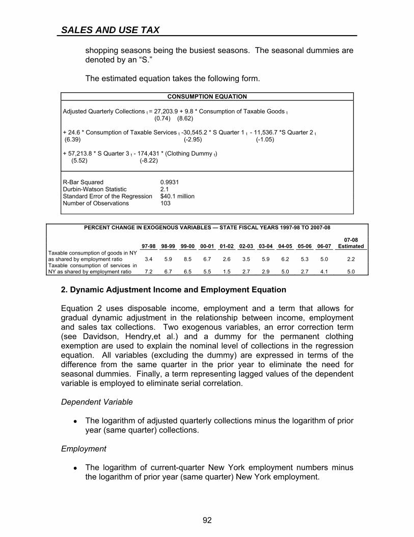
SALES AND USE TAX
92
shopping seasons being the busiest seasons. The seasonal dummies are denoted by an “S.”
The estimated equation takes the following form.
CONSUMPTION EQUATION Adjusted Quarterly Collections t = 27,203.9 + 9.8 * Consumption of Taxable Goods t (0.74) (8.62) + 24.6 * Consumption of Taxable Services t -30,545.2 * S Quarter 1 t - 11,536.7 *S Quarter 2 t (6.39) (-2.95) (-1.05) + 57,213.8 * S Quarter 3 t - 174,431 * (Clothing Dummy t) (5.52) (-8.22) R-Bar Squared 0.9931 Durbin-Watson Statistic 2.1 Standard Error of the Regression $40.1 million Number of Observations 103
PERCENT CHANGE IN EXOGENOUS VARIABLES — STATE FISCAL YEARS 1997-98 TO 2007-08
07-08 97-98 98-99 99-00 00-01 01-02 02-03 03-04 04-05 05-06 06-07 Estimated Taxable consumption of goods in NY as shared by employment ratio 3.4 5.9 8.5 6.7 2.6 3.5 5.9 6.2 5.3 5.0 2.2 Taxable consumption of services in NY as shared by employment ratio 7.2 6.7 6.5 5.5 1.5 2.7 2.9 5.0 2.7 4.1 5.0
2. Dynamic Adjustment Income and Employment Equation Equation 2 uses disposable income, employment and a term that allows for gradual dynamic adjustment in the relationship between income, employment and sales tax collections. Two exogenous variables, an error correction term (see Davidson, Hendry,et al.) and a dummy for the permanent clothing exemption are used to explain the nominal level of collections in the regression equation. All variables (excluding the dummy) are expressed in terms of the difference from the same quarter in the prior year to eliminate the need for seasonal dummies. Finally, a term representing lagged values of the dependent variable is employed to eliminate serial correlation. Dependent Variable
● The logarithm of adjusted quarterly collections minus the logarithm of prior year (same quarter) collections.
Employment
● The logarithm of current-quarter New York employment numbers minus the logarithm of prior year (same quarter) New York employment.
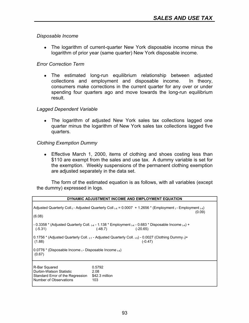
SALES AND USE TAX
93
Disposable Income
● The logarithm of current-quarter New York disposable income minus the logarithm of prior year (same quarter) New York disposable income.
Error Correction Term
● The estimated long-run equilibrium relationship between adjusted collections and employment and disposable income. In theory, consumers make corrections in the current quarter for any over or under spending four quarters ago and move towards the long-run equilibrium result.
Lagged Dependent Variable
● The logarithm of adjusted New York sales tax collections lagged one quarter minus the logarithm of New York sales tax collections lagged five quarters.
Clothing Exemption Dummy
● Effective March 1, 2000, items of clothing and shoes costing less than $110 are exempt from the sales and use tax. A dummy variable is set for the exemption. Weekly suspensions of the permanent clothing exemption are adjusted separately in the data set.
The form of the estimated equation is as follows, with all variables (except the dummy) expressed in logs.
DYNAMIC ADJUSTMENT INCOME AND EMPLOYMENT EQUATION Adjusted Quarterly Coll.t - Adjusted Quarterly Coll t-4 = 0.0007 + 1.2656 * (Employment t - Employment t-4) (0.09) (6.08) - 0.3358 * (Adjusted Quarterly Coll. t-4 - 1.138 * Employment t-4 - 0.683 * Disposable Income t-4) + (-5.31) (-48.7) (-20.65) 0.1756 * (Adjusted Quarterly Coll. t-1 - Adjusted Quarterly Coll. t-5) - 0.0027 (Clothing Dummy t)+ (1.88) (-0.47) 0.0776 * (Disposable Income t - Disposable Income t-4) (0.67) R-Bar Squared 0.5792 Durbin-Watson Statistic 2.08 Standard Error of the Regression $42.3 million Number of Observations 103
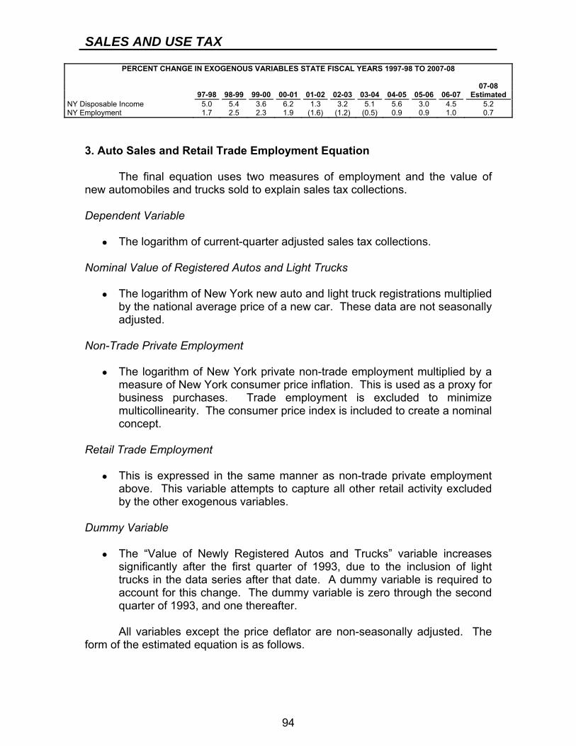
SALES AND USE TAX
94
PERCENT CHANGE IN EXOGENOUS VARIABLES STATE FISCAL YEARS 1997-98 TO 2007-08
07-08 97-98 98-99 99-00 00-01 01-02 02-03 03-04 04-05 05-06 06-07 Estimated NY Disposable Income 5.0 5.4 3.6 6.2 1.3 3.2 5.1 5.6 3.0 4.5 5.2 NY Employment 1.7 2.5 2.3 1.9 (1.6) (1.2) (0.5) 0.9 0.9 1.0 0.7
3. Auto Sales and Retail Trade Employment Equation The final equation uses two measures of employment and the value of new automobiles and trucks sold to explain sales tax collections. Dependent Variable
● The logarithm of current-quarter adjusted sales tax collections. Nominal Value of Registered Autos and Light Trucks
● The logarithm of New York new auto and light truck registrations multiplied by the national average price of a new car. These data are not seasonally adjusted.
Non-Trade Private Employment
● The logarithm of New York private non-trade employment multiplied by a measure of New York consumer price inflation. This is used as a proxy for business purchases. Trade employment is excluded to minimize multicollinearity. The consumer price index is included to create a nominal concept.
Retail Trade Employment
● This is expressed in the same manner as non-trade private employment above. This variable attempts to capture all other retail activity excluded by the other exogenous variables.
Dummy Variable
● The “Value of Newly Registered Autos and Trucks” variable increases significantly after the first quarter of 1993, due to the inclusion of light trucks in the data series after that date. A dummy variable is required to account for this change. The dummy variable is zero through the second quarter of 1993, and one thereafter.
All variables except the price deflator are non-seasonally adjusted. The form of the estimated equation is as follows.
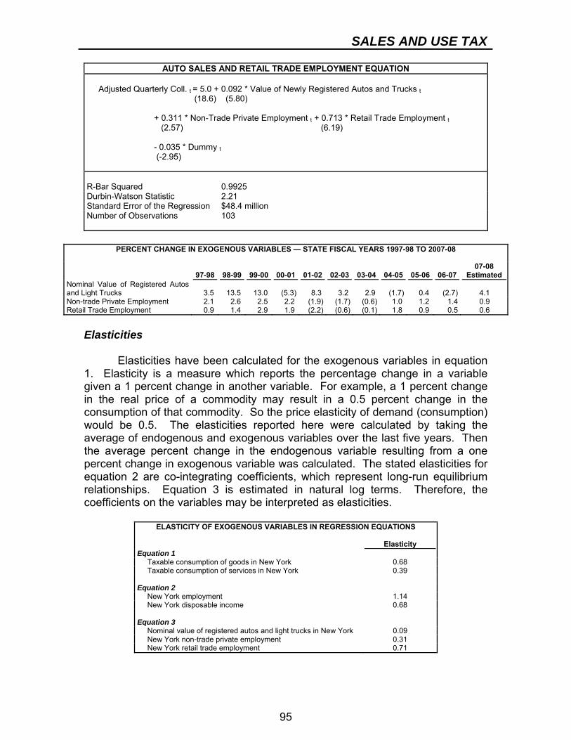
SALES AND USE TAX
95
AUTO SALES AND RETAIL TRADE EMPLOYMENT EQUATION Adjusted Quarterly Coll. t = 5.0 + 0.092 * Value of Newly Registered Autos and Trucks t (18.6) (5.80) + 0.311 * Non-Trade Private Employment t + 0.713 * Retail Trade Employment t (2.57) (6.19) - 0.035 * Dummy t (-2.95) R-Bar Squared 0.9925 Durbin-Watson Statistic 2.21 Standard Error of the Regression $48.4 million Number of Observations 103
PERCENT CHANGE IN EXOGENOUS VARIABLES — STATE FISCAL YEARS 1997-98 TO 2007-08
07-08 97-98 98-99 99-00 00-01 01-02 02-03 03-04 04-05 05-06 06-07 Estimated Nominal Value of Registered Autos and Light Trucks 3.5 13.5 13.0 (5.3) 8.3 3.2 2.9 (1.7) 0.4 (2.7) 4.1 Non-trade Private Employment 2.1 2.6 2.5 2.2 (1.9) (1.7) (0.6) 1.0 1.2 1.4 0.9 Retail Trade Employment 0.9 1.4 2.9 1.9 (2.2) (0.6) (0.1) 1.8 0.9 0.5 0.6
Elasticities Elasticities have been calculated for the exogenous variables in equation 1. Elasticity is a measure which reports the percentage change in a variable given a 1 percent change in another variable. For example, a 1 percent change in the real price of a commodity may result in a 0.5 percent change in the consumption of that commodity. So the price elasticity of demand (consumption) would be 0.5. The elasticities reported here were calculated by taking the average of endogenous and exogenous variables over the last five years. Then the average percent change in the endogenous variable resulting from a one percent change in exogenous variable was calculated. The stated elasticities for equation 2 are co-integrating coefficients, which represent long-run equilibrium relationships. Equation 3 is estimated in natural log terms. Therefore, the coefficients on the variables may be interpreted as elasticities.
ELASTICITY OF EXOGENOUS VARIABLES IN REGRESSION EQUATIONS
Elasticity Equation 1 Taxable consumption of goods in New York 0.68 Taxable consumption of services in New York 0.39 Equation 2 New York employment 1.14 New York disposable income 0.68 Equation 3 Nominal value of registered autos and light trucks in New York 0.09 New York non-trade private employment 0.31 New York retail trade employment 0.71
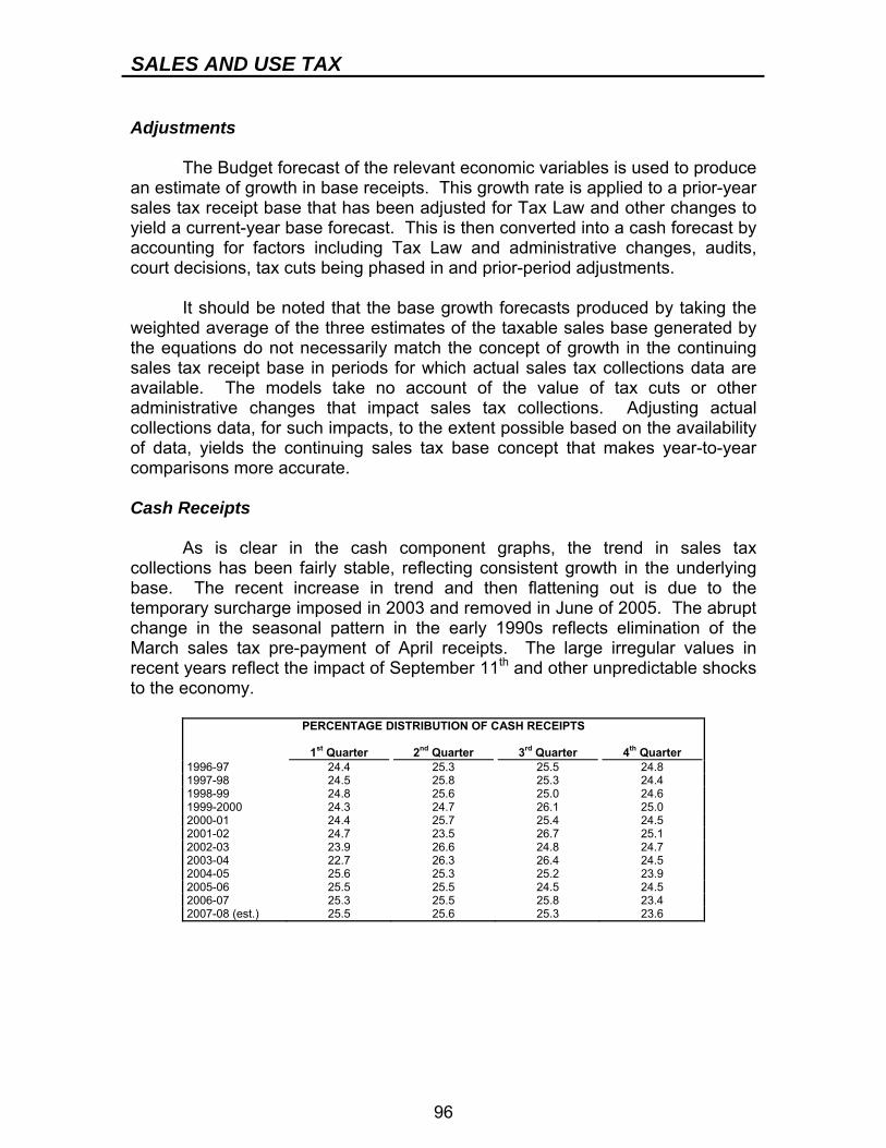
SALES AND USE TAX
96
Adjustments The Budget forecast of the relevant economic variables is used to produce an estimate of growth in base receipts. This growth rate is applied to a prior-year sales tax receipt base that has been adjusted for Tax Law and other changes to yield a current-year base forecast. This is then converted into a cash forecast by accounting for factors including Tax Law and administrative changes, audits, court decisions, tax cuts being phased in and prior-period adjustments. It should be noted that the base growth forecasts produced by taking the weighted average of the three estimates of the taxable sales base generated by the equations do not necessarily match the concept of growth in the continuing sales tax receipt base in periods for which actual sales tax collections data are available. The models take no account of the value of tax cuts or other administrative changes that impact sales tax collections. Adjusting actual collections data, for such impacts, to the extent possible based on the availability of data, yields the continuing sales tax base concept that makes year-to-year comparisons more accurate. Cash Receipts As is clear in the cash component graphs, the trend in sales tax collections has been fairly stable, reflecting consistent growth in the underlying base. The recent increase in trend and then flattening out is due to the temporary surcharge imposed in 2003 and removed in June of 2005. The abrupt change in the seasonal pattern in the early 1990s reflects elimination of the March sales tax pre-payment of April receipts. The large irregular values in recent years reflect the impact of September 11th and other unpredictable shocks to the economy.
PERCENTAGE DISTRIBUTION OF CASH RECEIPTS
1st Quarter 2nd Quarter 3rd Quarter 4th Quarter 1996-97 24.4 25.3 25.5 24.8 1997-98 24.5 25.8 25.3 24.4 1998-99 24.8 25.6 25.0 24.6 1999-2000 24.3 24.7 26.1 25.0 2000-01 24.4 25.7 25.4 24.5 2001-02 24.7 23.5 26.7 25.1 2002-03 23.9 26.6 24.8 24.7 2003-04 22.7 26.3 26.4 24.5 2004-05 25.6 25.3 25.2 23.9 2005-06 25.5 25.5 24.5 24.5 2006-07 25.3 25.5 25.8 23.4 2007-08 (est.) 25.5 25.6 25.3 23.6
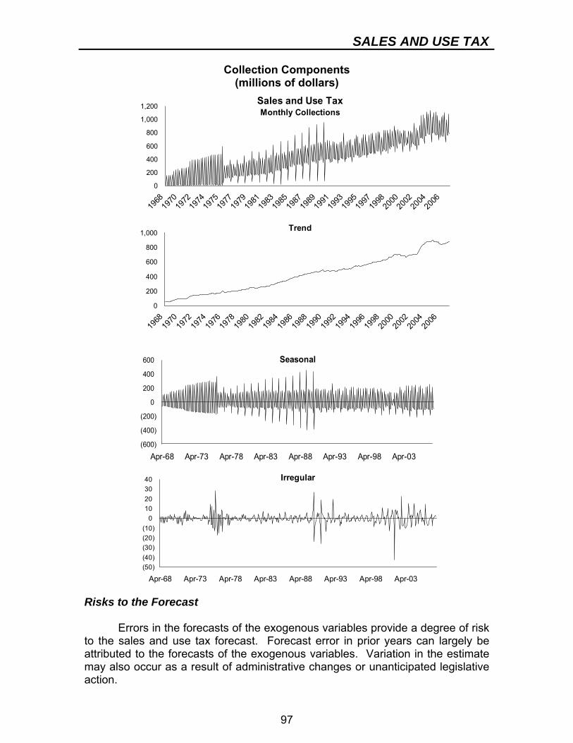
SALES AND USE TAX
97
Collection Components (millions of dollars)
0
200
400
600
800
1,000
1,200
1968
1970
1972
1974
1975
1977
1979
1981
1983
1985
1987
1989
1991
1993
1995
1997
1998
2000
2002
2004
2006
Sales and Use TaxMonthly Collections
0
200
400
600
800
1,000
1968
1970
1972
1974
1976
1978
1980
1982
1984
1986
1988
1990
1992
1994
1996
1998
2000
2002
2004
2006
Trend
(600)
(400)
(200)
0
200
400
600
Apr-68 Apr-73 Apr-78 Apr-83 Apr-88 Apr-93 Apr-98 Apr-03
Seasonal
(50)(40)(30)(20)(10)
010203040
Apr-68 Apr-73 Apr-78 Apr-83 Apr-88 Apr-93 Apr-98 Apr-03
Irregular
Risks to the Forecast Errors in the forecasts of the exogenous variables provide a degree of risk to the sales and use tax forecast. Forecast error in prior years can largely be attributed to the forecasts of the exogenous variables. Variation in the estimate may also occur as a result of administrative changes or unanticipated legislative action.
98
CIGARETTE AND TOBACCO TAXES TAX BASE AND RATE The New York State cigarette excise tax is imposed by Article 20 of the Tax Law on the sale or use of cigarettes within the State. The current tax rate is $1.50 per package of 20 cigarettes. The State also imposes a tax on other tobacco products, such as chewing tobacco, snuff, cigars, pipe tobacco and roll-your-own cigarette tobacco, at a rate of 37 percent of their wholesale price. Legislation passed with the Health Care Reform Act of 2000 increased the tax on the sale or use of cigarettes within the State by 55 cents to $1.11 per pack on March 1, 2000. Legislation enacted in 2002 raised the tax rate to $1.50 per pack beginning on April 3, 2002. The tax on tobacco products increased from 20 percent to 37 percent of wholesale price on July 2, 2002. Prior to June 1, 1993, the cigarette tax was 39 cents per pack and the tobacco products tax was 15 percent of wholesale price. The Federal government imposes a cigarette excise tax on manufacturers and first importers of cigarettes. The Federal tax rate, currently 39 cents per pack, was increased 24 cents to 34 cents per pack on January 1, 2000, and increased again to 39 cents per pack on January 1, 2002. New York City also levies a separate cigarette excise tax, which increased from 8 cents to $1.50 per pack on July 2, 2002. The Federal government also imposes an excise tax on manufacturers and importers of tobacco products at various rates, depending on the type of product. Sales on qualified Native American reservations to Native Americans are exempt from tax, along with sales to State and national governmental entities, the Armed Forces, the United Nations and diplomatic personnel. ADMINISTRATION State-registered stamping agents, who are mostly wholesalers, pay the excise tax through the purchase tax stamps from the State and affix the stamps to cigarette packages to be sold by New York State registered retailers. Out-of-State wholesalers may purchase cigarettes from a New York stamping agent without a State or joint City/State stamp affixed. New York residents who purchase non-stamped cigarettes, such as cigarettes purchased from out-of-State via the Internet or on Native American lands, must remit the cigarette excise tax directly to the Department of Taxation and Finance. An individual may bring two cartons into the State without being subject to the excise tax. DATA SOURCES The primary sources of data used in the estimation and forecasting of the cigarette and tobacco tax are as follows:
● AM043, Department of Taxation and Finance Monthly Report of Receipts. This report contains gross and net receipts data.
CIGARETTE AND TOBACCO TAXES
99
● New York State Department of Taxation and Finance Monthly and Fiscal Year Comparison of Cigarette Tax Collections. This report includes the number of stamps sold, assessments and agents’ commission.
● The Tax Burden on Tobacco. This annual data publication, previously published by the now-defunct Tobacco Institute, is produced by the economic consulting firm Orzechowski and Walker. It is the source of the consumption and cigarette price data used in the cigarette consumption forecasting equation.
● Various U.S. and New York government agencies provide the Consumer Price Index and population data used in the cigarette consumption equation.
● United States Department of Agriculture Economic Research Service, Tobacco Situation and Outlook Report. Published semi-annually. Used for national cigarette and tobacco products information.
● Campaign for Tobacco Free Kids. Various reports prepared by the Campaign for Tobacco Free Kids available on their web site.
STATUTORY CHANGES Tax rate changes have had the most significant impact on cigarette tax revenues. As shown in the accompanying graph, revenues spiked in the months following tax rate increases in 1972, 1983, 1989, 1990, 1993, 2000, and 2002 before slowing in the subsequent months. Total tax-paid cigarette consumption in New York has declined significantly since the mid-1980s. This is largely due to steady price increases, awareness of the adverse health consequences of smoking, smoking restrictions, anti-smoking programs, tax-free purchases on Indian reservations, lower tax rates in surrounding states, and bootlegging. Taxed consumption has also been affected by events including State, New York City and Federal cigarette tax increases, substantial enforcement efforts and the Tobacco Settlement. Major recent events affecting overall taxable consumption include:
● Increase in the New York City cigarette excise tax from 8 cents per pack to $1.50 per pack, effective July 2, 2002.
● Increase in the State cigarette tax from $1.11 per pack to $1.50 per pack, effective April 3, 2002.
● Increase in the State cigarette tax from 56 cents per pack to $1.11 per pack, effective March 1, 2000.
● Additional 18 cents per pack price increase and full-year impact of the 45 cents per pack price increase in 1999-2000, due primarily to the cost of the Master Tobacco Settlement Agreement on the industry.
● Ten-cent Federal excise tax increase, resulting in a 13 cent wholesale price increase in the last quarter of State fiscal year 1999-2000.
● Doubling of New Jersey’s cigarette excise tax and part-year impact of a 45 cent price increase resulting from the Tobacco Settlement in 1998-99.
● State enforcement program enacted in 1997-98.
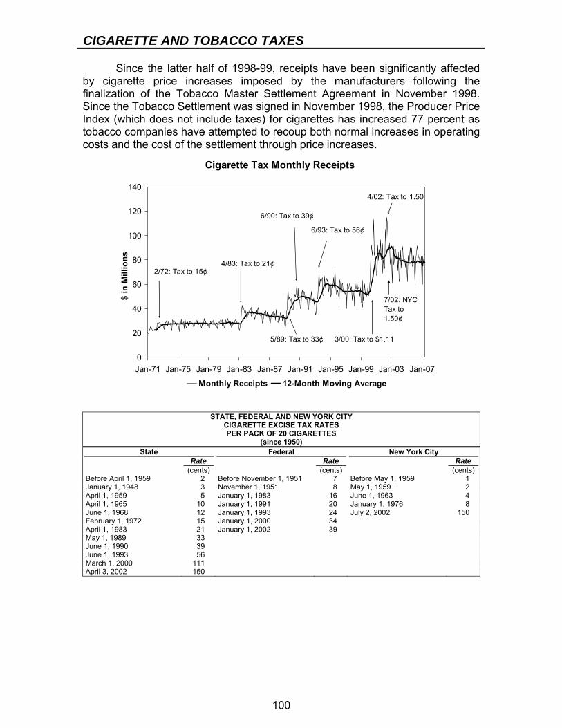
CIGARETTE AND TOBACCO TAXES
100
Since the latter half of 1998-99, receipts have been significantly affected by cigarette price increases imposed by the manufacturers following the finalization of the Tobacco Master Settlement Agreement in November 1998. Since the Tobacco Settlement was signed in November 1998, the Producer Price Index (which does not include taxes) for cigarettes has increased 77 percent as tobacco companies have attempted to recoup both normal increases in operating costs and the cost of the settlement through price increases.
Cigarette Tax Monthly Receipts
0
20
40
60
80
100
120
140
Jan-71 Jan-75 Jan-79 Jan-83 Jan-87 Jan-91 Jan-95 Jan-99 Jan-03 Jan-07
$ in
Mill
ions
Monthly Receipts 12-Month Moving Average
2/72: Tax to 15¢4/83: Tax to 21¢
5/89: Tax to 33¢
6/90: Tax to 39¢
6/93: Tax to 56¢
3/00: Tax to $1.11
4/02: Tax to 1.50
7/02: NYC Tax to 1.50¢
STATE, FEDERAL AND NEW YORK CITY CIGARETTE EXCISE TAX RATES PER PACK OF 20 CIGARETTES
(since 1950) State Federal New York City
Rate (cents)
Rate (cents)
Rate (cents)
Before April 1, 1959 2 Before November 1, 1951 7 Before May 1, 1959 1 January 1, 1948 3 November 1, 1951 8 May 1, 1959 2 April 1, 1959 5 January 1, 1983 16 June 1, 1963 4 April 1, 1965 10 January 1, 1991 20 January 1, 1976 8 June 1, 1968 12 January 1, 1993 24 July 2, 2002 150 February 1, 1972 15 January 1, 2000 34 April 1, 1983 21 January 1, 2002 39 May 1, 1989 33 June 1, 1990 39 June 1, 1993 56 March 1, 2000 111 April 3, 2002 150
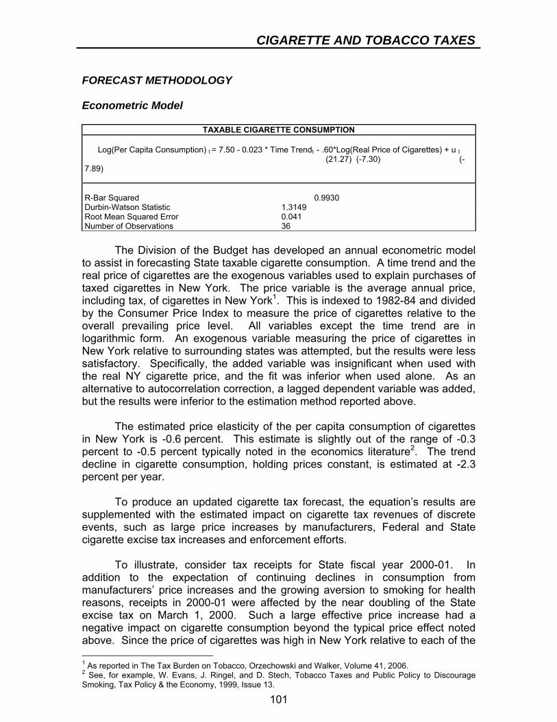
CIGARETTE AND TOBACCO TAXES
101
FORECAST METHODOLOGY Econometric Model
TAXABLE CIGARETTE CONSUMPTION
Log(Per Capita Consumption) t = 7.50 - 0.023 * Time Trendt - .60*Log(Real Price of Cigarettes) + u t (21.27) (-7.30) (-7.89) R-Bar Squared 0.9930 Durbin-Watson Statistic 1.3149 Root Mean Squared Error 0.041 Number of Observations 36 The Division of the Budget has developed an annual econometric model to assist in forecasting State taxable cigarette consumption. A time trend and the real price of cigarettes are the exogenous variables used to explain purchases of taxed cigarettes in New York. The price variable is the average annual price, including tax, of cigarettes in New York1. This is indexed to 1982-84 and divided by the Consumer Price Index to measure the price of cigarettes relative to the overall prevailing price level. All variables except the time trend are in logarithmic form. An exogenous variable measuring the price of cigarettes in New York relative to surrounding states was attempted, but the results were less satisfactory. Specifically, the added variable was insignificant when used with the real NY cigarette price, and the fit was inferior when used alone. As an alternative to autocorrelation correction, a lagged dependent variable was added, but the results were inferior to the estimation method reported above. The estimated price elasticity of the per capita consumption of cigarettes in New York is -0.6 percent. This estimate is slightly out of the range of -0.3 percent to -0.5 percent typically noted in the economics literature2. The trend decline in cigarette consumption, holding prices constant, is estimated at -2.3 percent per year. To produce an updated cigarette tax forecast, the equation’s results are supplemented with the estimated impact on cigarette tax revenues of discrete events, such as large price increases by manufacturers, Federal and State cigarette excise tax increases and enforcement efforts. To illustrate, consider tax receipts for State fiscal year 2000-01. In addition to the expectation of continuing declines in consumption from manufacturers’ price increases and the growing aversion to smoking for health reasons, receipts in 2000-01 were affected by the near doubling of the State excise tax on March 1, 2000. Such a large effective price increase had a negative impact on cigarette consumption beyond the typical price effect noted above. Since the price of cigarettes was high in New York relative to each of the 1 As reported in The Tax Burden on Tobacco, Orzechowski and Walker, Volume 41, 2006. 2 See, for example, W. Evans, J. Ringel, and D. Stech, Tobacco Taxes and Public Policy to Discourage Smoking, Tax Policy & the Economy, 1999, Issue 13.
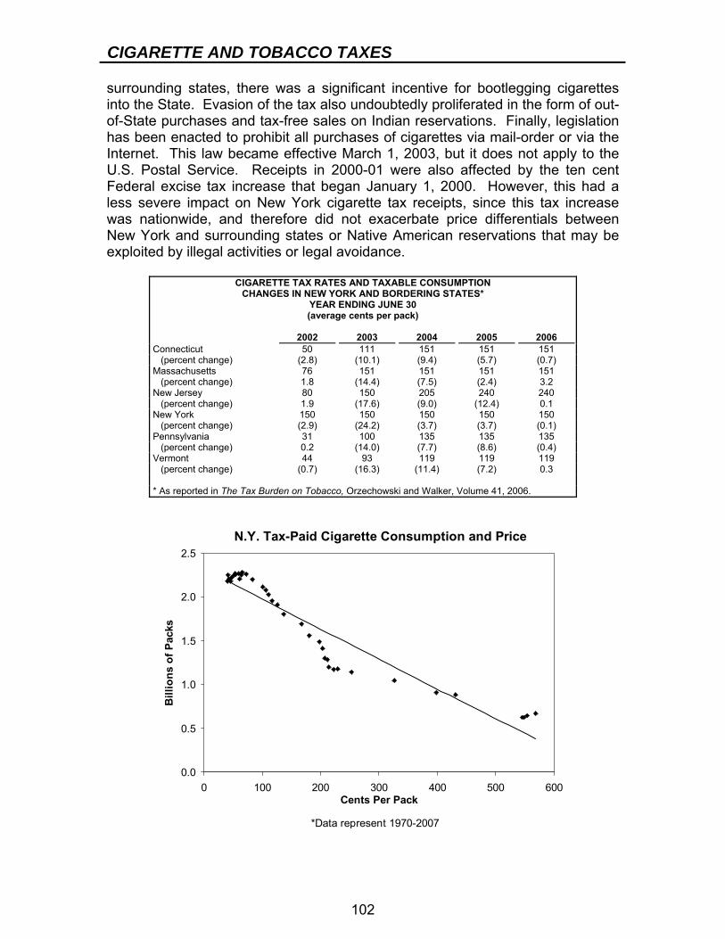
CIGARETTE AND TOBACCO TAXES
102
surrounding states, there was a significant incentive for bootlegging cigarettes into the State. Evasion of the tax also undoubtedly proliferated in the form of out-of-State purchases and tax-free sales on Indian reservations. Finally, legislation has been enacted to prohibit all purchases of cigarettes via mail-order or via the Internet. This law became effective March 1, 2003, but it does not apply to the U.S. Postal Service. Receipts in 2000-01 were also affected by the ten cent Federal excise tax increase that began January 1, 2000. However, this had a less severe impact on New York cigarette tax receipts, since this tax increase was nationwide, and therefore did not exacerbate price differentials between New York and surrounding states or Native American reservations that may be exploited by illegal activities or legal avoidance.
CIGARETTE TAX RATES AND TAXABLE CONSUMPTION CHANGES IN NEW YORK AND BORDERING STATES*
YEAR ENDING JUNE 30 (average cents per pack)
2002 2003 2004 2005 2006 Connecticut 50 111 151 151 151 (percent change) (2.8) (10.1) (9.4) (5.7) (0.7) Massachusetts 76 151 151 151 151 (percent change) 1.8 (14.4) (7.5) (2.4) 3.2 New Jersey 80 150 205 240 240 (percent change) 1.9 (17.6) (9.0) (12.4) 0.1 New York 150 150 150 150 150 (percent change) (2.9) (24.2) (3.7) (3.7) (0.1) Pennsylvania 31 100 135 135 135 (percent change) 0.2 (14.0) (7.7) (8.6) (0.4) Vermont 44 93 119 119 119 (percent change) (0.7) (16.3) (11.4) (7.2) 0.3 * As reported in The Tax Burden on Tobacco, Orzechowski and Walker, Volume 41, 2006.
N.Y. Tax-Paid Cigarette Consumption and Price
0.0
0.5
1.0
1.5
2.0
2.5
0 100 200 300 400 500 600Cents Per Pack
Bill
ions
of P
acks
*Data represent 1970-2007
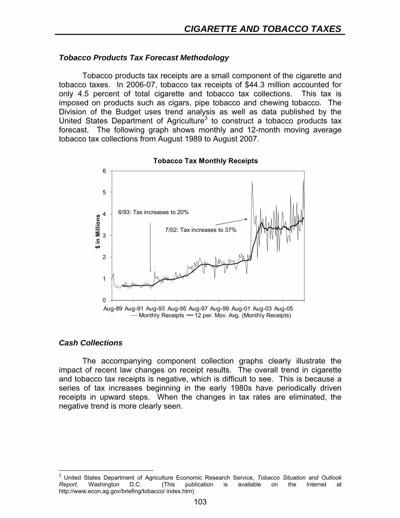
CIGARETTE AND TOBACCO TAXES
103
Tobacco Products Tax Forecast Methodology Tobacco products tax receipts are a small component of the cigarette and tobacco taxes. In 2006-07, tobacco tax receipts of $44.3 million accounted for only 4.5 percent of total cigarette and tobacco tax collections. This tax is imposed on products such as cigars, pipe tobacco and chewing tobacco. The Division of the Budget uses trend analysis as well as data published by the United States Department of Agriculture3 to construct a tobacco products tax forecast. The following graph shows monthly and 12-month moving average tobacco tax collections from August 1989 to August 2007.
Tobacco Tax Monthly Receipts
0
1
2
3
4
5
6
Aug-89 Aug-91 Aug-93 Aug-95 Aug-97 Aug-99 Aug-01 Aug-03 Aug-05
$ in
Mill
ions
Monthly Receipts 12 per. Mov. Avg. (Monthly Receipts)
6/93: Tax increases to 20%
7/02: Tax increases to 37%
Cash Collections The accompanying component collection graphs clearly illustrate the impact of recent law changes on receipt results. The overall trend in cigarette and tobacco tax receipts is negative, which is difficult to see. This is because a series of tax increases beginning in the early 1980s have periodically driven receipts in upward steps. When the changes in tax rates are eliminated, the negative trend is more clearly seen.
3 United States Department of Agriculture Economic Research Service, Tobacco Situation and Outlook Report, Washington D.C. (This publication is available on the Internet at http://www.econ.ag.gov/briefing/tobacco/ index.htm)
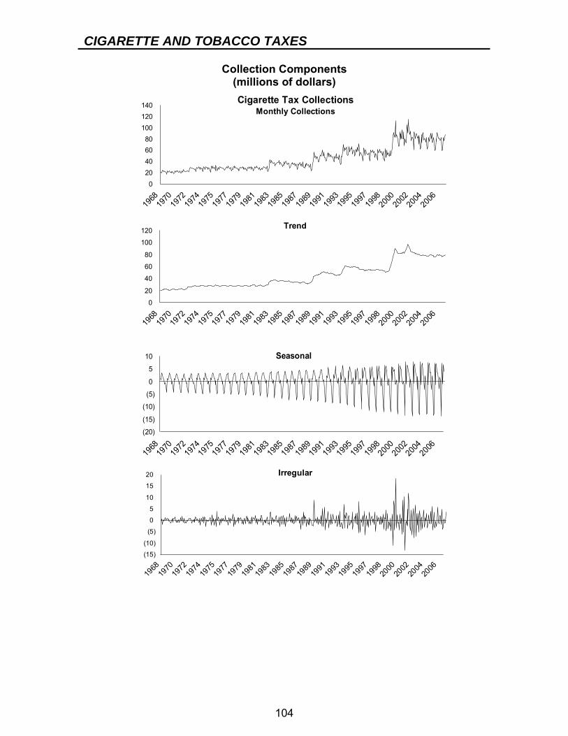
CIGARETTE AND TOBACCO TAXES
104
Collection Components (millions of dollars)
020406080
100120140
1968
1970
1972
1974
1975
1977
1979
1981
1983
1985
1987
1989
1991
1993
1995
1997
1998
2000
2002
2004
2006
Cigarette Tax CollectionsMonthly Collections
0
20
40
60
80
100
120
1968
1970
1972
1974
1975
1977
1979
1981
1983
1985
1987
1989
1991
1993
1995
1997
1998
2000
2002
2004
2006
Trend
(20)
(15)
(10)
(5)
0
5
10
1968
1970
1972
1974
1975
1977
1979
1981
1983
1985
1987
1989
1991
199319
9519
9719
9820
0020
02200
420
06
Seasonal
(15)
(10)
(5)
0
5
10
15
20
1968
1970
1972
1974
1975
1977
1979
1981
1983
1985
1987
1989
1991
1993
1995
1997
1998
2000
2002
2004
2006
Irregular
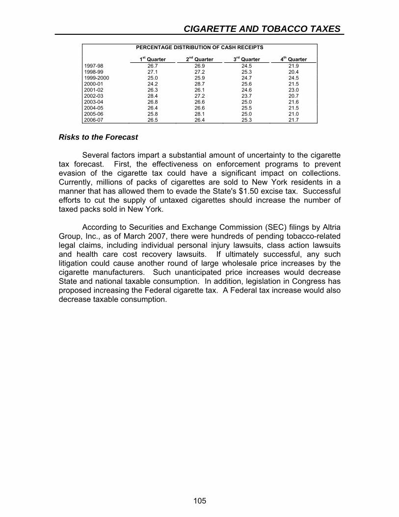
CIGARETTE AND TOBACCO TAXES
105
PERCENTAGE DISTRIBUTION OF CASH RECEIPTS
1st Quarter 2nd Quarter 3rd Quarter 4th Quarter 1997-98 26.7 26.9 24.5 21.9 1998-99 27.1 27.2 25.3 20.4 1999-2000 25.0 25.9 24.7 24.5 2000-01 24.2 28.7 25.6 21.5 2001-02 26.3 26.1 24.6 23.0 2002-03 28.4 27.2 23.7 20.7 2003-04 26.8 26.6 25.0 21.6 2004-05 26.4 26.6 25.5 21.5 2005-06 25.8 28.1 25.0 21.0 2006-07 26.5 26.4 25.3 21.7
Risks to the Forecast Several factors impart a substantial amount of uncertainty to the cigarette tax forecast. First, the effectiveness on enforcement programs to prevent evasion of the cigarette tax could have a significant impact on collections. Currently, millions of packs of cigarettes are sold to New York residents in a manner that has allowed them to evade the State's $1.50 excise tax. Successful efforts to cut the supply of untaxed cigarettes should increase the number of taxed packs sold in New York. According to Securities and Exchange Commission (SEC) filings by Altria Group, Inc., as of March 2007, there were hundreds of pending tobacco-related legal claims, including individual personal injury lawsuits, class action lawsuits and health care cost recovery lawsuits. If ultimately successful, any such litigation could cause another round of large wholesale price increases by the cigarette manufacturers. Such unanticipated price increases would decrease State and national taxable consumption. In addition, legislation in Congress has proposed increasing the Federal cigarette tax. A Federal tax increase would also decrease taxable consumption.
106
MOTOR FUEL TAX BACKGROUND Tax Base and Rate An 8 cent-per-gallon tax is imposed on the sale of gasoline and diesel motor fuel in the State. Prior to January 1, 1996, the diesel motor fuel tax was 10 cents per gallon. Non-highway uses of motor fuel, such as in construction machinery, agricultural machinery, commercial vessels, or vehicles operated on rails or tracks, are granted refunds of the tax. Thus, the tax is levied primarily on fuel used in motor vehicles operating on the public highways of the State or fuel used in recreational boats on the State’s waterways. Since 2003-04, all motor fuel tax receipts are earmarked to the Dedicated Highway and Bridge Trust Fund and the Dedicated Mass Transportation Trust Fund. No monies are directed to the General Fund. Administration The gasoline component of the motor fuel tax is remitted upon first import for sale, use, storage or distribution in New York State. The diesel motor fuel tax is collected on the first non-exempt sale in the State. The tax is generally remitted monthly, although vendors whose average monthly tax is less than $200 may remit quarterly. Vendors with annual tax liability of more than $5 million for both the motor fuel tax and the petroleum business tax during the preceding year must remit the tax via electronic funds transfer (EFT) or by certified check by the third business day following the 22nd of each month. DATA SOURCES The primary sources of data used in the estimation and forecasting for the motor fuel tax are as follows:
● AM043, Department of Taxation and Finance Monthly Report of Receipts. This report contains gross and net receipts data.
● United States Energy Information Administration. Various publications, including the Short Term Energy Outlook, Petroleum Marketing Monthly and Annual Energy and Motor Gasoline Watch, contain useful information. These are available on the Internet at http://www.eia.doe.gov.
● Various U.S. and New York government agencies, including the U.S. Bureau of Economic Analysis of the Commerce Department. These agencies provide economic data used to develop gasoline and diesel consumption forecasts.
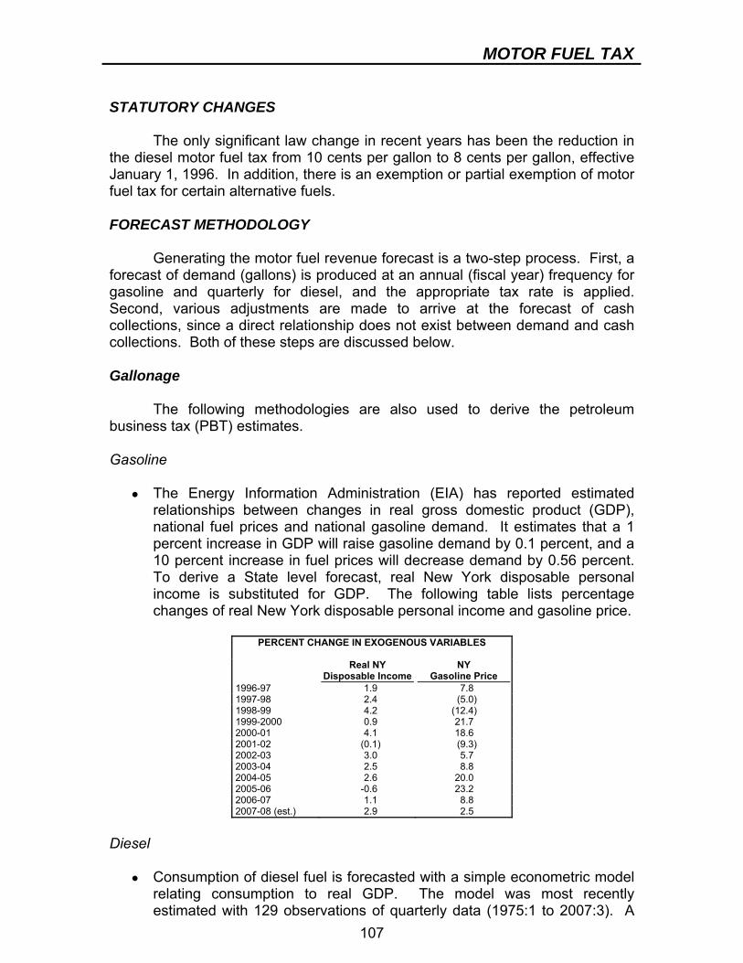
MOTOR FUEL TAX
107
STATUTORY CHANGES The only significant law change in recent years has been the reduction in the diesel motor fuel tax from 10 cents per gallon to 8 cents per gallon, effective January 1, 1996. In addition, there is an exemption or partial exemption of motor fuel tax for certain alternative fuels. FORECAST METHODOLOGY Generating the motor fuel revenue forecast is a two-step process. First, a forecast of demand (gallons) is produced at an annual (fiscal year) frequency for gasoline and quarterly for diesel, and the appropriate tax rate is applied. Second, various adjustments are made to arrive at the forecast of cash collections, since a direct relationship does not exist between demand and cash collections. Both of these steps are discussed below. Gallonage The following methodologies are also used to derive the petroleum business tax (PBT) estimates. Gasoline
● The Energy Information Administration (EIA) has reported estimated relationships between changes in real gross domestic product (GDP), national fuel prices and national gasoline demand. It estimates that a 1 percent increase in GDP will raise gasoline demand by 0.1 percent, and a 10 percent increase in fuel prices will decrease demand by 0.56 percent. To derive a State level forecast, real New York disposable personal income is substituted for GDP. The following table lists percentage changes of real New York disposable personal income and gasoline price.
PERCENT CHANGE IN EXOGENOUS VARIABLES
Real NY
Disposable IncomeNY
Gasoline Price 1996-97 1.9 7.8 1997-98 2.4 (5.0) 1998-99 4.2 (12.4) 1999-2000 0.9 21.7 2000-01 4.1 18.6 2001-02 (0.1) (9.3) 2002-03 3.0 5.7 2003-04 2.5 8.8 2004-05 2.6 20.0 2005-06 -0.6 23.2 2006-07 1.1 8.8 2007-08 (est.) 2.9 2.5
Diesel
● Consumption of diesel fuel is forecasted with a simple econometric model relating consumption to real GDP. The model was most recently estimated with 129 observations of quarterly data (1975:1 to 2007:3). A
MOTOR FUEL TAX
108
dummy variable is used to isolate the impact of changes in tax remittance in State fiscal year 1988-89. A quarterly dummy variable for the first calendar quarter is also used to reflect quarterly consumption patterns.
Adjustments After generating a demand forecast and applying the appropriate tax rates, adjustments are made for refunds, audits, credits, pay schedule lags, accounting delays, historical and year-to-date collection patterns and tax law and administrative changes.
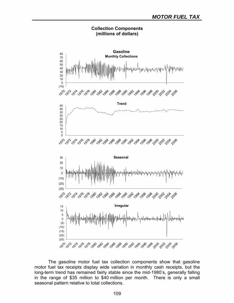
MOTOR FUEL TAX
109
Collection Components (millions of dollars)
(10)0
1020304050607080
1970
1972
1974
1976
1978
1980
1982
1984
1986
1988
1990
1992
1994
1996
1998
2000
2002
2004
2006
GasolineMonthly Collections
05
1015202530354045
1970
1972
1974
1976
1978
1980
1982
1984
1986
1988
1990
1992
1994
1996
1998
2000
2002
2004
2006
Trend
(30)
(20)
(10)
0
10
20
30
1970
1972
1974
1976
1978
1980
1982
1984
1986
1988
1990
1992
1994
1996
1998
2000
2002
2004
2006
Seasonal
(25)(20)(15)(10)
(5)05
1015
1970
1972
1974
1976
1978
1980
1982
1984
1986
1988
1990
1992
1994
1996
1998
2000
2002
2004
2006
Irregular
The gasoline motor fuel tax collection components show that gasoline motor fuel tax receipts display wide variation in monthly cash receipts, but the long-term trend has remained fairly stable since the mid-1980’s, generally falling in the range of $35 million to $40 million per month. There is only a small seasonal pattern relative to total collections.
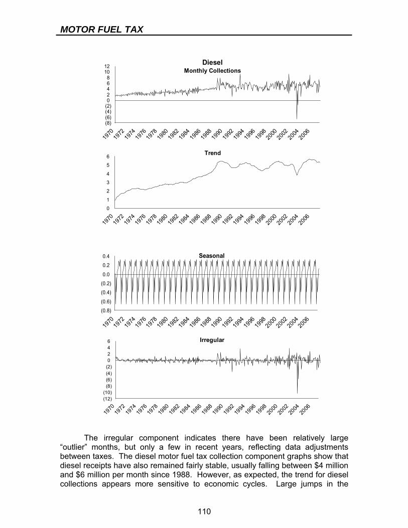
MOTOR FUEL TAX
110
(8)(6)(4)(2)02468
1012
1970
1972
1974
1976
1978
1980
1982
1984
1986
1988
1990
1992
1994
1996
1998
2000
2002
2004
2006
DieselMonthly Collections
0
1
2
3
4
5
6
1970
1972
1974
1976
1978
1980
1982
1984
1986
1988
1990
1992
1994
1996
1998
2000
2002
2004
2006
Trend
(0.8)
(0.6)
(0.4)
(0.2)
0.0
0.2
0.4
1970
1972
1974
1976
1978
1980
1982
1984
1986
1988
1990
1992
1994
1996
1998
2000
2002
2004
2006
Seasonal
(12)(10)
(8)(6)(4)(2)0246
1970
1972
1974
1976
1978
1980
1982
1984
1986
1988
1990
1992
1994
1996
1998
2000
2002
2004
2006
Irregular
The irregular component indicates there have been relatively large “outlier” months, but only a few in recent years, reflecting data adjustments between taxes. The diesel motor fuel tax collection component graphs show that diesel receipts have also remained fairly stable, usually falling between $4 million and $6 million per month since 1988. However, as expected, the trend for diesel collections appears more sensitive to economic cycles. Large jumps in the
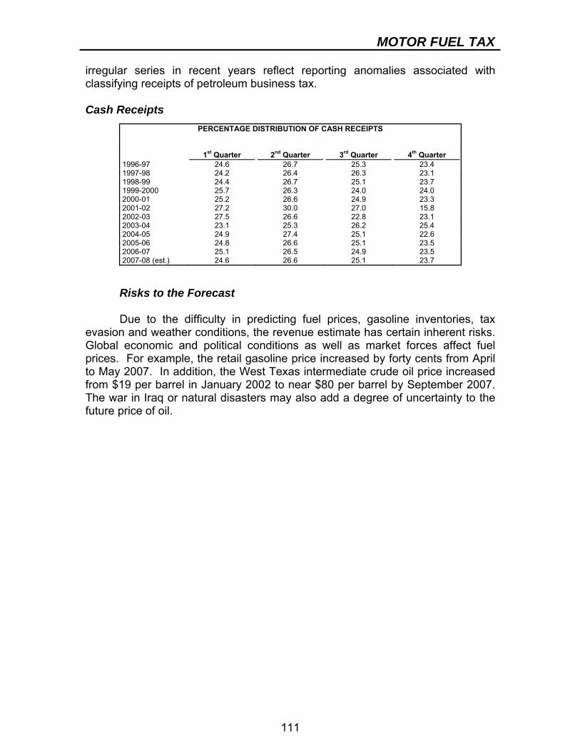
MOTOR FUEL TAX
111
irregular series in recent years reflect reporting anomalies associated with classifying receipts of petroleum business tax. Cash Receipts Risks to the Forecast Due to the difficulty in predicting fuel prices, gasoline inventories, tax evasion and weather conditions, the revenue estimate has certain inherent risks. Global economic and political conditions as well as market forces affect fuel prices. For example, the retail gasoline price increased by forty cents from April to May 2007. In addition, the West Texas intermediate crude oil price increased from $19 per barrel in January 2002 to near $80 per barrel by September 2007. The war in Iraq or natural disasters may also add a degree of uncertainty to the future price of oil.
PERCENTAGE DISTRIBUTION OF CASH RECEIPTS
1st Quarter 2nd Quarter 3rd Quarter 4th Quarter 1996-97 24.6 26.7 25.3 23.4 1997-98 24.2 26.4 26.3 23.1 1998-99 24.4 26.7 25.1 23.7 1999-2000 25.7 26.3 24.0 24.0 2000-01 25.2 26.6 24.9 23.3 2001-02 27.2 30.0 27.0 15.8 2002-03 27.5 26.6 22.8 23.1 2003-04 23.1 25.3 26.2 25.4 2004-05 24.9 27.4 25.1 22.6 2005-06 24.8 26.6 25.1 23.5 2006-07 25.1 26.5 24.9 23.5 2007-08 (est.) 24.6 26.6 25.1 23.7

112
MOTOR VEHICLE FEES BACKGROUND Motor vehicle fees are imposed by the Vehicle and Traffic Law. An early version, enacted in 1929, was itself derived from other laws pertaining to traffic, such as the General Highway Traffic Law. The latest codification, which with subsequent amendments remains current, was enacted in 1959 and became effective in October 1960. Tax Base and Rate Motor vehicle fees are derived from a variety of sources, but consist mainly of vehicle registration and driver licensing fees. Most vehicle registration fees are based on vehicle weight, but buses are charged according to seating capacity and semi-trailers are charged a flat fee. Registration for vehicles weighing less than 18,000 pounds is biennial. Drivers’ licenses are originally issued for five years and renewals for eight-year periods. Basic renewal rates, per annum, are $5 for an operator’s license, $10 for a chauffeur’s license, and $15 for a commercial driver’s license. Numerous other fees, related to the processes of registration or licensing, are also components of motor vehicle fees. Such fees include inspection and emission stickers, repair shop certificates, and insurance civil penalties. Administration Registration and licensing take place at the central and district offices of the Department of Motor Vehicles and by mail and at county clerks’ offices in most counties. DATA SOURCES The primary source of data is Preliminary Motor Vehicle Transactions, Department of Motor Vehicles. This report contains monthly data on item volume and dollar receipts. STATUTORY CHANGES The main statutory or administrative changes that have a bearing on the history of actual cash receipts include:
● extension of license renewal period from four to five years (1996-97); ● change in method and rate for paying county clerks (1996-97); ● extension of validity of original licenses from four to five years (1997-98); ● increase in the photo image fee (1997-98); ● reduction of 25 percent in graduated rates on passenger cars (1998-99); ● extension of license renewal period from five to eight years (2000-01);

MOTOR VEHICLE FEES
113
● re-issuance of license plates (2000-01 through 2002-03) ● increase in title fees (2004-05); and ● reclassification of certain fees (2005-06).
FORECAST METHODOLOGY Since the preponderant parts of motor vehicle fees are registrations (70 percent) and licenses (20 percent), most attention is paid to the following variables:
● the number of passenger and commercial vehicles and the average weight of each type;
● the number of new and renewal licenses; and ● the cyclical pattern of registration, licensing, and renewal.
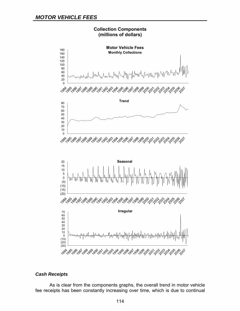
MOTOR VEHICLE FEES
114
Collection Components (millions of dollars)
020406080
100120140160180
1984
1985
1986
1987
1988
1989
1990
1991
1992
1993
1994
1995
1996
1997
1998
1999
2000
2001
2002
2003
2004
2005
2006
2007
Motor Vehicle FeesMonthly Collections
01020304050607080
1984
1985
1986
1987
1988
1989
1990
1991
1992
1993
1994
1995
1996
1997
1998
1999
2000
2001
2002
2003
2004
2005
2006
2007
Trend
(20)(15)(10)(5)05
101520
1984
1985
1986
1987
1988
1989
1990
199119
9219
9319
9419
9519
9619
9719
9819
99200
020
0120
0220
0320
0420
0520
0620
07
Seasonal
(30)(20)(10)
010203040506070
1984
1985
1986
1987
1988
1989
1990
1991
1992
1993
1994
1995
1996
1997
1998
1999
2000
2001
2002
2003
2004
2005
2006
2007
Irregular
Cash Receipts As is clear from the components graphs, the overall trend in motor vehicle fee receipts has been constantly increasing over time, which is due to continual

MOTOR VEHICLE FEES
115
increases in various fees. There is a pronounced seasonal pattern with peaks during the summer months. The irregular component is relatively large compared to trend. The cash forecast is developed by growing the existing base using estimated growth in registrations and licenses. Furthermore, the statutory or administrative changes pertaining to any variable (see Statutory Changes) are taken into account. The table below illustrates quarterly cash flow for motor vehicle fees on an All Funds basis.
PERCENTAGE DISTRIBUTION OF CASH RECEIPTS
1st Quarter 2nd Quarter 3rd Quarter 4th Quarter 1996-97 26.3 22.3 25.3 26.1 1997-98 26.3 25.4 25.0 23.3 1998-99 31.2 23.5 20.1 25.2 1999-2000 23.6 26.0 24.4 26.0 2000-01 29.3 23.1 21.1 26.5 2001-02 26.1 23.9 25.0 25.0 2002-03 29.1 21.5 24.6 24.8 2003-04 27.9 25.5 22.4 24.2 2004-05 29.4 25.5 24.4 20.7 2005-06 21.4 19.4 23.8 35.4 2006-07 (est.) 28.0 23.0 25.7 24.7
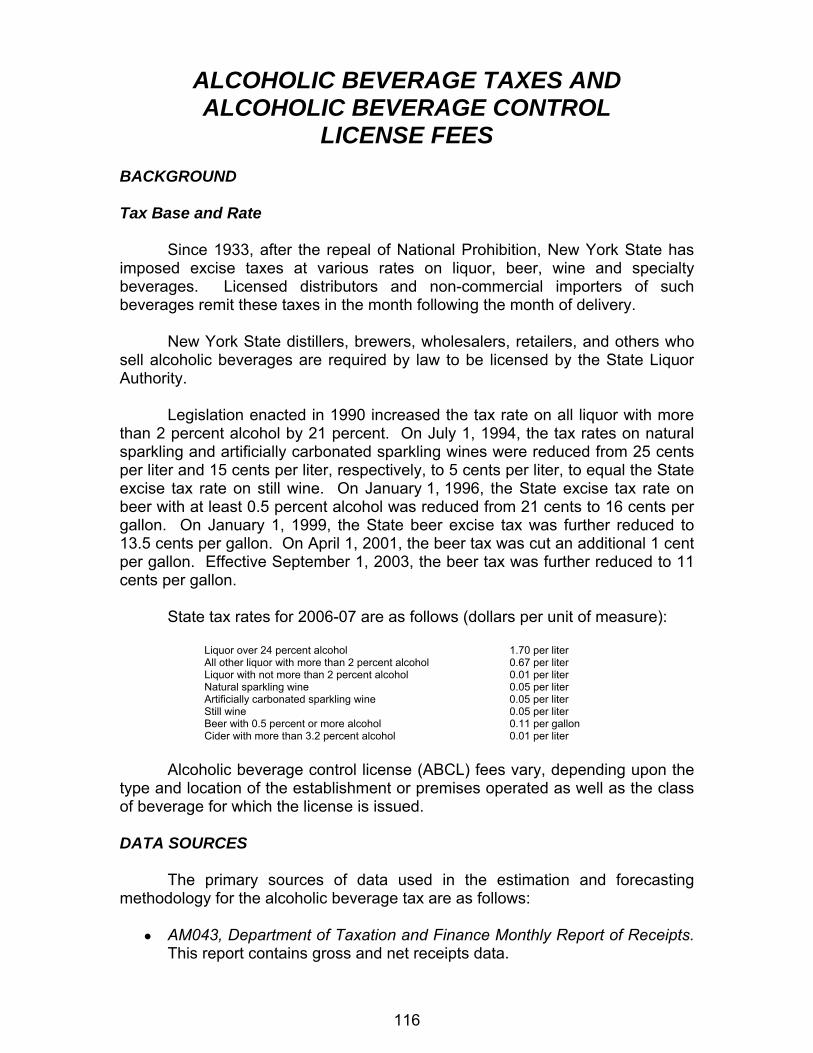
116
ALCOHOLIC BEVERAGE TAXES AND ALCOHOLIC BEVERAGE CONTROL
LICENSE FEES BACKGROUND Tax Base and Rate Since 1933, after the repeal of National Prohibition, New York State has imposed excise taxes at various rates on liquor, beer, wine and specialty beverages. Licensed distributors and non-commercial importers of such beverages remit these taxes in the month following the month of delivery. New York State distillers, brewers, wholesalers, retailers, and others who sell alcoholic beverages are required by law to be licensed by the State Liquor Authority. Legislation enacted in 1990 increased the tax rate on all liquor with more than 2 percent alcohol by 21 percent. On July 1, 1994, the tax rates on natural sparkling and artificially carbonated sparkling wines were reduced from 25 cents per liter and 15 cents per liter, respectively, to 5 cents per liter, to equal the State excise tax rate on still wine. On January 1, 1996, the State excise tax rate on beer with at least 0.5 percent alcohol was reduced from 21 cents to 16 cents per gallon. On January 1, 1999, the State beer excise tax was further reduced to 13.5 cents per gallon. On April 1, 2001, the beer tax was cut an additional 1 cent per gallon. Effective September 1, 2003, the beer tax was further reduced to 11 cents per gallon. State tax rates for 2006-07 are as follows (dollars per unit of measure):
Liquor over 24 percent alcohol 1.70 per liter All other liquor with more than 2 percent alcohol 0.67 per liter Liquor with not more than 2 percent alcohol 0.01 per liter Natural sparkling wine 0.05 per liter Artificially carbonated sparkling wine 0.05 per liter Still wine 0.05 per liter Beer with 0.5 percent or more alcohol 0.11 per gallon Cider with more than 3.2 percent alcohol 0.01 per liter
Alcoholic beverage control license (ABCL) fees vary, depending upon the type and location of the establishment or premises operated as well as the class of beverage for which the license is issued. DATA SOURCES The primary sources of data used in the estimation and forecasting methodology for the alcoholic beverage tax are as follows:
● AM043, Department of Taxation and Finance Monthly Report of Receipts. This report contains gross and net receipts data.
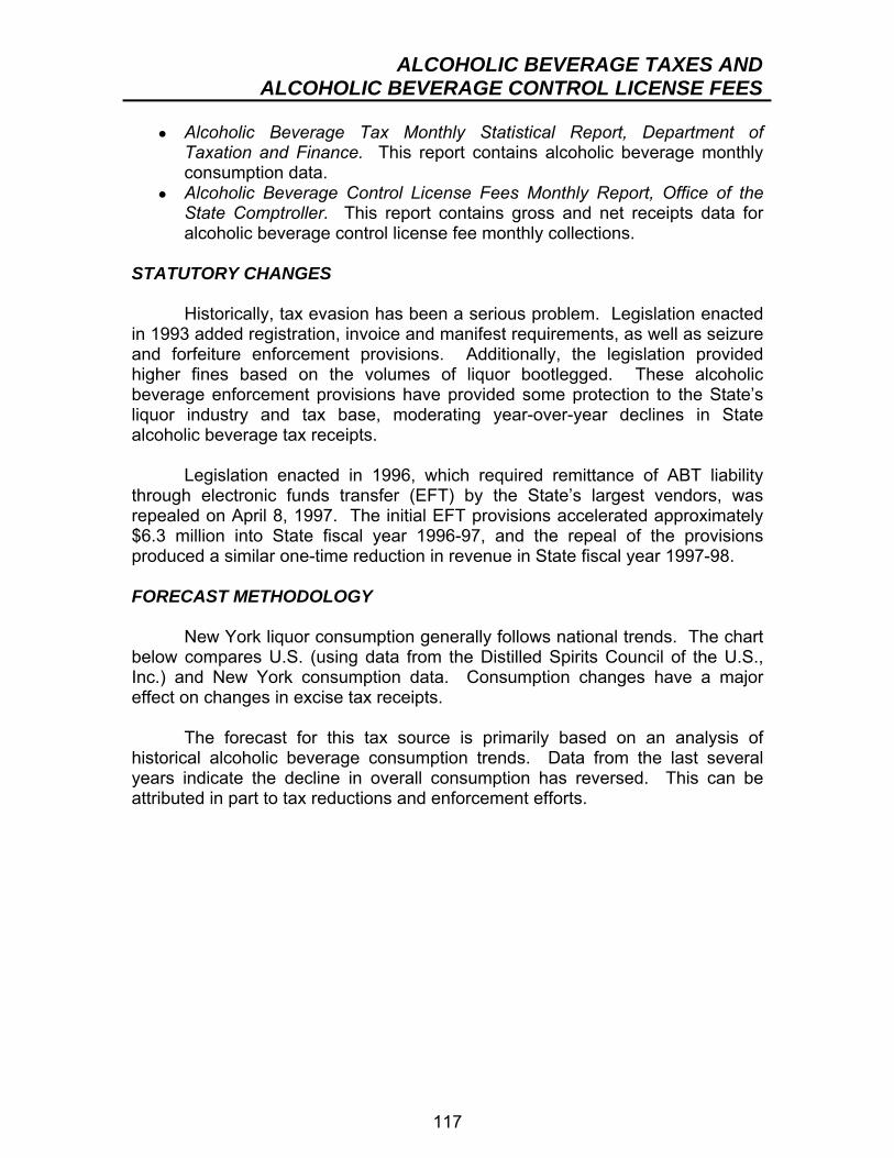
ALCOHOLIC BEVERAGE TAXES ANDALCOHOLIC BEVERAGE CONTROL LICENSE FEES
117
● Alcoholic Beverage Tax Monthly Statistical Report, Department of Taxation and Finance. This report contains alcoholic beverage monthly consumption data.
● Alcoholic Beverage Control License Fees Monthly Report, Office of the State Comptroller. This report contains gross and net receipts data for alcoholic beverage control license fee monthly collections.
STATUTORY CHANGES Historically, tax evasion has been a serious problem. Legislation enacted in 1993 added registration, invoice and manifest requirements, as well as seizure and forfeiture enforcement provisions. Additionally, the legislation provided higher fines based on the volumes of liquor bootlegged. These alcoholic beverage enforcement provisions have provided some protection to the State’s liquor industry and tax base, moderating year-over-year declines in State alcoholic beverage tax receipts. Legislation enacted in 1996, which required remittance of ABT liability through electronic funds transfer (EFT) by the State’s largest vendors, was repealed on April 8, 1997. The initial EFT provisions accelerated approximately $6.3 million into State fiscal year 1996-97, and the repeal of the provisions produced a similar one-time reduction in revenue in State fiscal year 1997-98. FORECAST METHODOLOGY New York liquor consumption generally follows national trends. The chart below compares U.S. (using data from the Distilled Spirits Council of the U.S., Inc.) and New York consumption data. Consumption changes have a major effect on changes in excise tax receipts. The forecast for this tax source is primarily based on an analysis of historical alcoholic beverage consumption trends. Data from the last several years indicate the decline in overall consumption has reversed. This can be attributed in part to tax reductions and enforcement efforts.
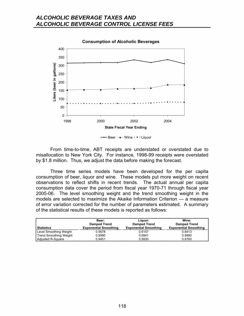
ALCOHOLIC BEVERAGE TAXES AND ALCOHOLIC BEVERAGE CONTROL LICENSE FEES
118
Consumption of Alcoholic Beverages
0
50
100
150
200
250
300
350
400
1998 2000 2002 2004
State Fiscal Year Ending
Lite
rs (b
eer i
n ga
llons
)
Beer Wine Liquor From time-to-time, ABT receipts are understated or overstated due to misallocation to New York City. For instance, 1998-99 receipts were overstated by $1.8 million. Thus, we adjust the data before making the forecast. Three time series models have been developed for the per capita consumption of beer, liquor and wine. These models put more weight on recent observations to reflect shifts in recent trends. The actual annual per capita consumption data cover the period from fiscal year 1970-71 through fiscal year 2005-06. The level smoothing weight and the trend smoothing weight in the models are selected to maximize the Akaike Information Criterion — a measure of error variation corrected for the number of parameters estimated. A summary of the statistical results of these models is reported as follows: Statistics
Beer: Damped Trend
Exponential Smoothing
Liquor: Damped Trend
Exponential Smoothing
Wine: Damped Trend
Exponential Smoothing Level Smoothing Weight 0.5678 0.6157 0.8413 Trend Smoothing Weight 0.9990 0.6941 0.9990 Adjusted R-Square 0.9451 0.9930 0.8760
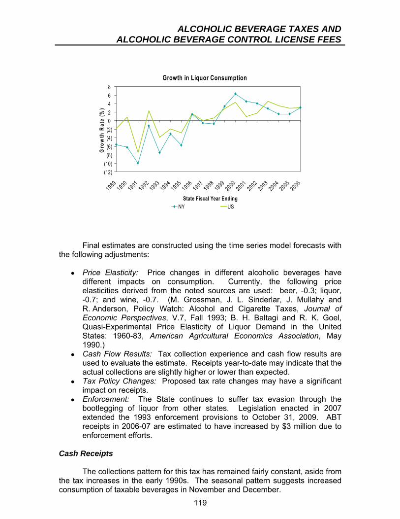
ALCOHOLIC BEVERAGE TAXES ANDALCOHOLIC BEVERAGE CONTROL LICENSE FEES
119
Growth in Liquor Consumption
(12)(10)
(8)(6)(4)(2)02468
19891990
19911992
19931994
19951996
19971998
19992000
20012002
20032004
20052006
State Fiscal Year Ending
Gro
wth
Rat
e (%
)
NY US
Final estimates are constructed using the time series model forecasts with the following adjustments:
● Price Elasticity: Price changes in different alcoholic beverages have different impacts on consumption. Currently, the following price elasticities derived from the noted sources are used: beer, -0.3; liquor, -0.7; and wine, -0.7. (M. Grossman, J. L. Sinderlar, J. Mullahy and R. Anderson, Policy Watch: Alcohol and Cigarette Taxes, Journal of Economic Perspectives, V.7, Fall 1993; B. H. Baltagi and R. K. Goel, Quasi-Experimental Price Elasticity of Liquor Demand in the United States: 1960-83, American Agricultural Economics Association, May 1990.)
● Cash Flow Results: Tax collection experience and cash flow results are used to evaluate the estimate. Receipts year-to-date may indicate that the actual collections are slightly higher or lower than expected.
● Tax Policy Changes: Proposed tax rate changes may have a significant impact on receipts.
● Enforcement: The State continues to suffer tax evasion through the bootlegging of liquor from other states. Legislation enacted in 2007 extended the 1993 enforcement provisions to October 31, 2009. ABT receipts in 2006-07 are estimated to have increased by $3 million due to enforcement efforts.
Cash Receipts The collections pattern for this tax has remained fairly constant, aside from the tax increases in the early 1990s. The seasonal pattern suggests increased consumption of taxable beverages in November and December.
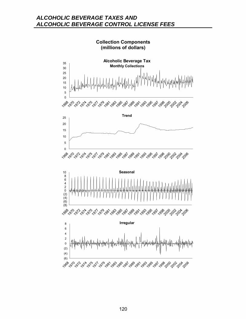
ALCOHOLIC BEVERAGE TAXES AND ALCOHOLIC BEVERAGE CONTROL LICENSE FEES
120
Collection Components
(millions of dollars)
05
101520253035
1968
1970
1972
1974
1975
1977
1979
1981
1983
1985
1987
1989
1991
1993
1995
1997
1998
2000
2002
2004
2006
Alcoholic Beverage TaxMonthly Collections
0
5
10
15
20
25
1968
1970
1972
1974
1975
1977
1979
1981
1983
1985
1987
1989
1991
1993
1995
1997
1998
2000
2002
2004
2006
Trend
(8)(6)(4)(2)02468
10
1968
1970
1972
1974
1975
1977
1979
1981
1983
1985
1987
1989
1991
199319
9519
9719
9820
0020
02200
420
06
Seasonal
(6)
(4)
(2)
0
2
4
6
8
1968
1970
1972
1974
1975
1977
1979
1981
1983
1985
1987
1989
1991
1993
1995
1997
1998
2000
2002
2004
2006
Irregular
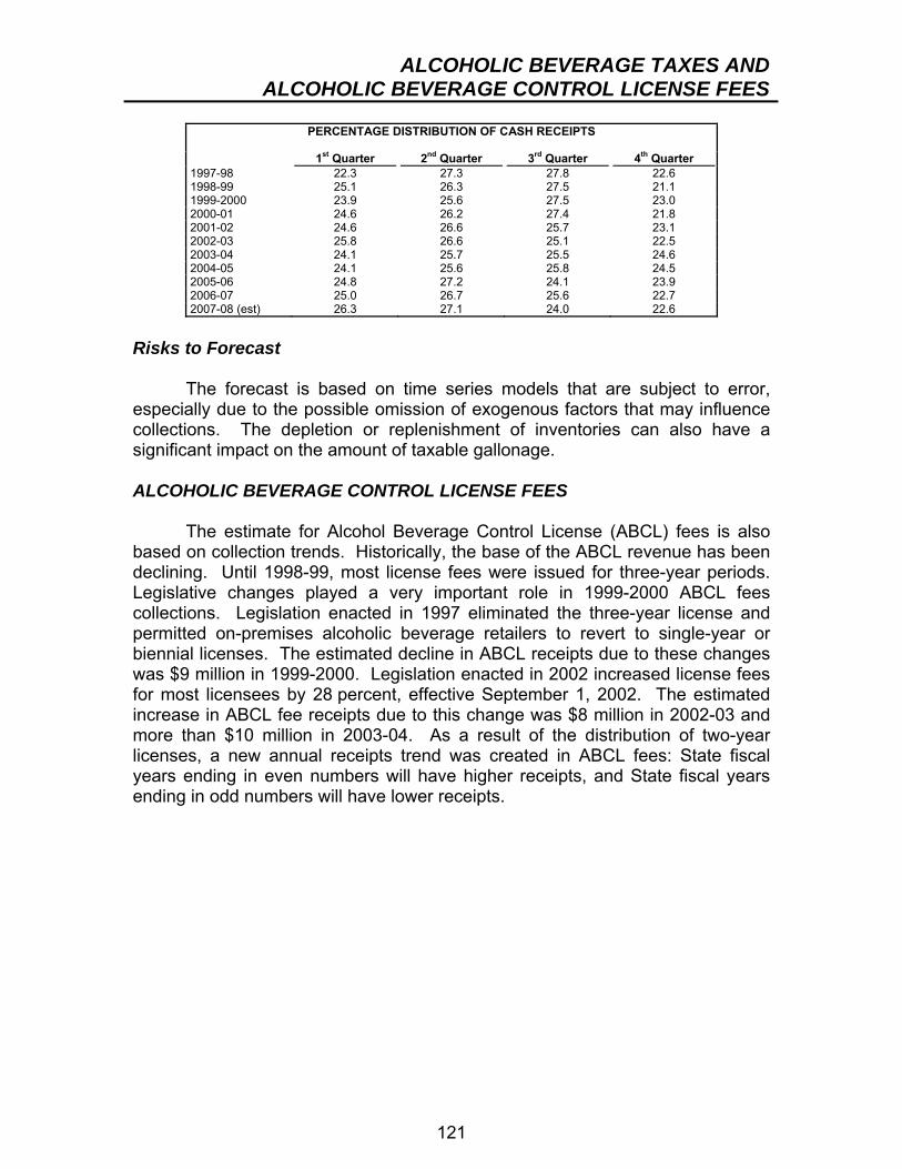
ALCOHOLIC BEVERAGE TAXES ANDALCOHOLIC BEVERAGE CONTROL LICENSE FEES
121
PERCENTAGE DISTRIBUTION OF CASH RECEIPTS
1st Quarter 2nd Quarter 3rd Quarter 4th Quarter 1997-98 22.3 27.3 27.8 22.6 1998-99 25.1 26.3 27.5 21.1 1999-2000 23.9 25.6 27.5 23.0 2000-01 24.6 26.2 27.4 21.8 2001-02 24.6 26.6 25.7 23.1 2002-03 25.8 26.6 25.1 22.5 2003-04 24.1 25.7 25.5 24.6 2004-05 24.1 25.6 25.8 24.5 2005-06 24.8 27.2 24.1 23.9 2006-07 25.0 26.7 25.6 22.7 2007-08 (est) 26.3 27.1 24.0 22.6
Risks to Forecast The forecast is based on time series models that are subject to error, especially due to the possible omission of exogenous factors that may influence collections. The depletion or replenishment of inventories can also have a significant impact on the amount of taxable gallonage. ALCOHOLIC BEVERAGE CONTROL LICENSE FEES The estimate for Alcohol Beverage Control License (ABCL) fees is also based on collection trends. Historically, the base of the ABCL revenue has been declining. Until 1998-99, most license fees were issued for three-year periods. Legislative changes played a very important role in 1999-2000 ABCL fees collections. Legislation enacted in 1997 eliminated the three-year license and permitted on-premises alcoholic beverage retailers to revert to single-year or biennial licenses. The estimated decline in ABCL receipts due to these changes was $9 million in 1999-2000. Legislation enacted in 2002 increased license fees for most licensees by 28 percent, effective September 1, 2002. The estimated increase in ABCL fee receipts due to this change was $8 million in 2002-03 and more than $10 million in 2003-04. As a result of the distribution of two-year licenses, a new annual receipts trend was created in ABCL fees: State fiscal years ending in even numbers will have higher receipts, and State fiscal years ending in odd numbers will have lower receipts.
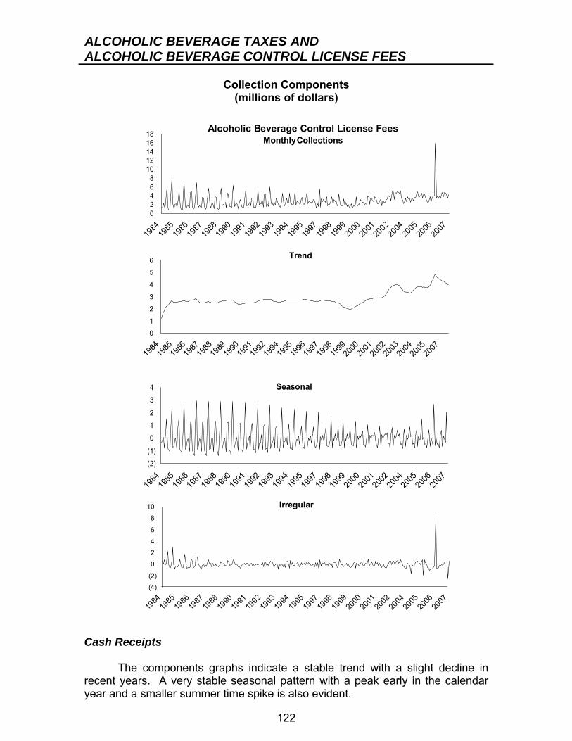
ALCOHOLIC BEVERAGE TAXES AND ALCOHOLIC BEVERAGE CONTROL LICENSE FEES
122
Collection Components (millions of dollars)
02468
1012141618
1984
1985
1986
1987
1988
1990
1991
1992
1993
1994
1995
1997
1998
1999
2000
2001
2002
2004
2005
2006
2007
Alcoholic Beverage Control License Fees Monthly Collections
0
1
2
3
4
5
6
1984
1985
1986
1987
1988
1989
1990
1991
1992
1994
1995
1996
1997
1998
1999
2000
2001
2002
2003
2004
2005
2007
Trend
(2)
(1)
0
1
2
3
4
1984
1985
1986
1987
1988
1990
1991
1992
1993
1994
1995
1997
1998
1999
2000
2001
2002
2004
2005
2006
2007
Seasonal
(4)
(2)
0
2
4
6
8
10
1984
1985
1986
1987
1988
1990
1991
1992
1993
1994
1995
1997
1998
1999
2000
2001
2002
2004
2005
2006
2007
Irregular
Cash Receipts The components graphs indicate a stable trend with a slight decline in recent years. A very stable seasonal pattern with a peak early in the calendar year and a smaller summer time spike is also evident.
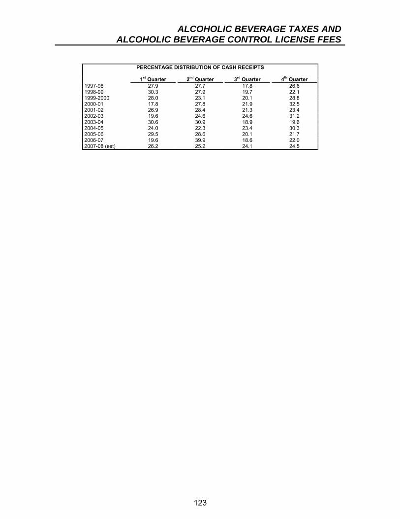
ALCOHOLIC BEVERAGE TAXES ANDALCOHOLIC BEVERAGE CONTROL LICENSE FEES
123
PERCENTAGE DISTRIBUTION OF CASH RECEIPTS
1st Quarter 2nd Quarter 3rd Quarter 4th Quarter 1997-98 27.9 27.7 17.8 26.6 1998-99 30.3 27.9 19.7 22.1 1999-2000 28.0 23.1 20.1 28.8 2000-01 17.8 27.8 21.9 32.5 2001-02 26.9 28.4 21.3 23.4 2002-03 19.6 24.6 24.6 31.2 2003-04 30.6 30.9 18.9 19.6 2004-05 24.0 22.3 23.4 30.3 2005-06 29.5 28.6 20.1 21.7 2006-07 19.6 39.9 18.6 22.0 2007-08 (est) 26.2 25.2 24.1 24.5
124
HIGHWAY USE TAX BACKGROUND Tax Base and Rate A highway use tax is imposed on commercial vehicles using the public highways of the State. The highway use tax (HUT) includes three components: the truck mileage tax, the fuel use tax, and a highway use registration system. All highway use tax receipts are earmarked to the Dedicated Highway and Bridge Trust Fund. The truck mileage tax (TMT) is levied on commercial vehicles having a loaded gross weight of more than 18,000 pounds or, at the option of the carrier, an unloaded weight in excess of 8,000 pounds for trucks and 4,000 pounds for tractors. The tax is imposed at rates graduated according to gross vehicle weight. The tax is calculated by multiplying the number of “laden” or “unladen” miles traveled on public highways of the State by the appropriate tax rate. The fuel use tax is a complement to the motor fuel tax and the sales tax and is levied on commercial vehicles. In contrast to the motor fuel tax, which is imposed on the amount of fuel purchased within the State, the fuel use tax is imposed on fuel purchased outside but used within New York. This tax is levied on the basis of the number of miles traveled on the public highways of the State. The aggregate fuel use tax rate is the sum of the appropriate motor fuel tax rate and the sales tax rate. The statewide rate for the sales tax component is equal to the State rate of 8 cents per gallon for motor fuel and diesel motor fuel plus the lowest county sales tax rate. A credit or refund is allowed for motor fuel tax or sales tax paid on fuels purchased but not used within the State. Commercial carriers, who are liable for the TMT, must purchase a certificate of registration. In 2007, the registration system replaced the permit system in order to adhere to a 2005 Federal transportation bill. This bill stated that States were no longer authorized to issue highway use tax permits. The registration system is based on the license plate number of a vehicle. The cost structure has not changed. The Commissioner of Taxation and Finance could deny registration if the carrier has not paid monies due from any other tax. There is now a civil penalty for any person who fails to obtain a certificate of registration when it is required. Administration Most taxpayers remit the TMT on a monthly basis. The tax is remitted on or before the last day of each month for the proceeding month. Fuel use taxpayers file quarterly with their home state under the rules of the International Fuel Use Tax Agreement (IFTA). The home state subsequently distributes the funds to the state where the liability occurred. The highway use permits are currently issued and renewed every three years.
HIGHWAY USE TAX
125
DATA SOURCES The primary sources of data used in the estimation and forecasting methodology for the highway use tax are as follows:
● AM043, Department of Taxation and Finance Monthly Report of Receipts. This report contains gross and net receipts data.
● Various U.S. and New York government agencies, including the U.S. Bureau of Economic Analysis of the Commerce Department. These agencies provide economic data used in the econometric equation.
STATUTORY CHANGES Truck Mileage Tax Since 1951, the TMT has been levied on commercial vehicles having a loaded gross weight of more than 18,000 pounds. In 1961, the State gave carriers the option of using an unloaded weight basis to compute truck mileage tax liability. A motor carrier pays tax based on both the number of miles driven on the public highways of this State and the weight of the vehicle. For State fiscal years 1990-91 through 1992-93, the economic recession suppressed the demand for trucking. However, 1990 legislative changes contributed to large increases in highway use tax receipts. Legislation enacted in 1990 applied the truck mileage tax to New York State Thruway mileage. It also imposed a supplemental tax that effectively doubled truck mileage tax rates for all roadways other than the Thruway. Legislation enacted in 1994 reduced the truck mileage tax rates imposed on New York State Thruway mileage by one-half and eliminated such rates on January 1, 1996. The supplemental tax rate was reduced by 50 percent on January 1, 1999 (1998 legislation), and an additional 20 percent on April 1, 2001 (2000 legislation). Fuel Use Tax Legislation in 1977 expanded the fuel use tax to include a sales and use tax component. This law change altered the impact of fuel price changes on fuel use tax receipts. Based on this law, increases in fuel prices inhibited fuel consumption, thereby lowering tax collections; in contrast, price increases raised the sales tax component rate and thereby fuel use tax collections. Legislation in 1994 permitted taxpayers who purchase more fuel in New York State than they consume in the State to claim refunds or credits for all excess payments of State fuel use taxes beginning January 1, 1995, and authorized the State to join the federally mandated International Fuel Tax Agreement (IFTA) on January 1, 1996. Legislation in 1995 reduced the automotive diesel fuel excise tax rate from 10 cents per gallon to 8 cents per gallon. As a result, the diesel fuel tax
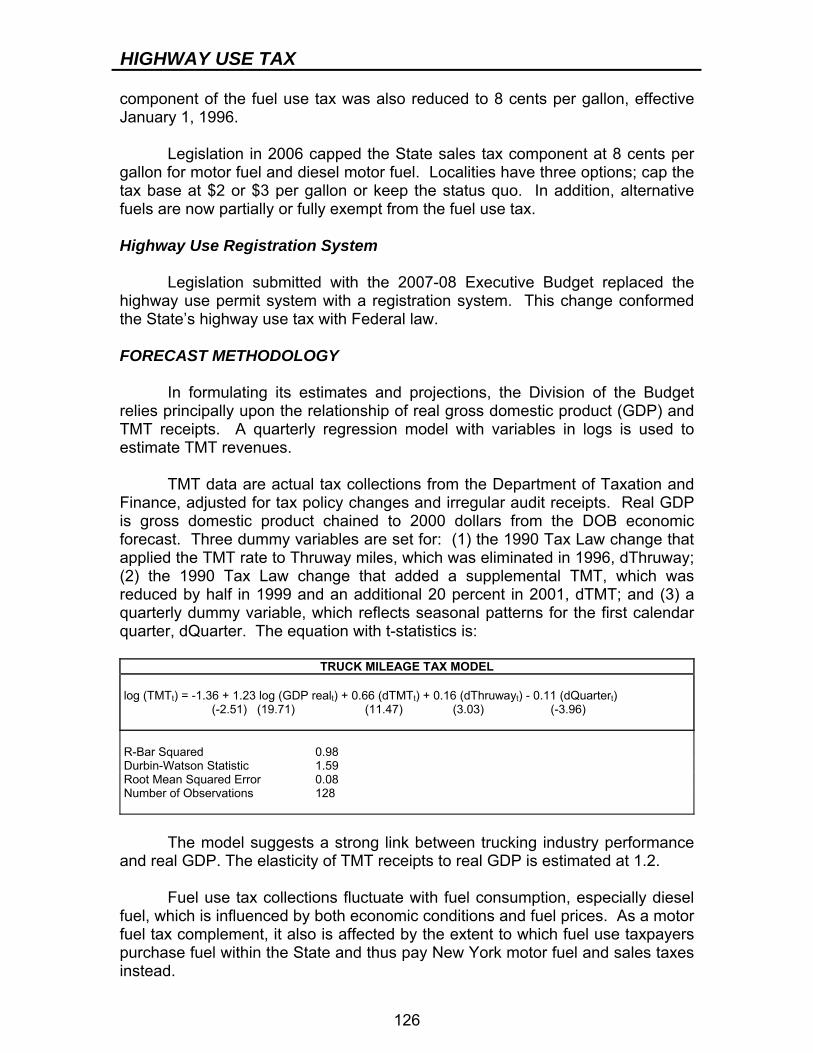
HIGHWAY USE TAX
126
component of the fuel use tax was also reduced to 8 cents per gallon, effective January 1, 1996. Legislation in 2006 capped the State sales tax component at 8 cents per gallon for motor fuel and diesel motor fuel. Localities have three options; cap the tax base at $2 or $3 per gallon or keep the status quo. In addition, alternative fuels are now partially or fully exempt from the fuel use tax. Highway Use Registration System Legislation submitted with the 2007-08 Executive Budget replaced the highway use permit system with a registration system. This change conformed the State’s highway use tax with Federal law. FORECAST METHODOLOGY In formulating its estimates and projections, the Division of the Budget relies principally upon the relationship of real gross domestic product (GDP) and TMT receipts. A quarterly regression model with variables in logs is used to estimate TMT revenues. TMT data are actual tax collections from the Department of Taxation and Finance, adjusted for tax policy changes and irregular audit receipts. Real GDP is gross domestic product chained to 2000 dollars from the DOB economic forecast. Three dummy variables are set for: (1) the 1990 Tax Law change that applied the TMT rate to Thruway miles, which was eliminated in 1996, dThruway; (2) the 1990 Tax Law change that added a supplemental TMT, which was reduced by half in 1999 and an additional 20 percent in 2001, dTMT; and (3) a quarterly dummy variable, which reflects seasonal patterns for the first calendar quarter, dQuarter. The equation with t-statistics is:
TRUCK MILEAGE TAX MODEL log (TMTt) = -1.36 + 1.23 log (GDP realt) + 0.66 (dTMTt) + 0.16 (dThruwayt) - 0.11 (dQuartert) (-2.51) (19.71) (11.47) (3.03) (-3.96) R-Bar Squared 0.98 Durbin-Watson Statistic 1.59 Root Mean Squared Error 0.08 Number of Observations 128 The model suggests a strong link between trucking industry performance and real GDP. The elasticity of TMT receipts to real GDP is estimated at 1.2. Fuel use tax collections fluctuate with fuel consumption, especially diesel fuel, which is influenced by both economic conditions and fuel prices. As a motor fuel tax complement, it also is affected by the extent to which fuel use taxpayers purchase fuel within the State and thus pay New York motor fuel and sales taxes instead.
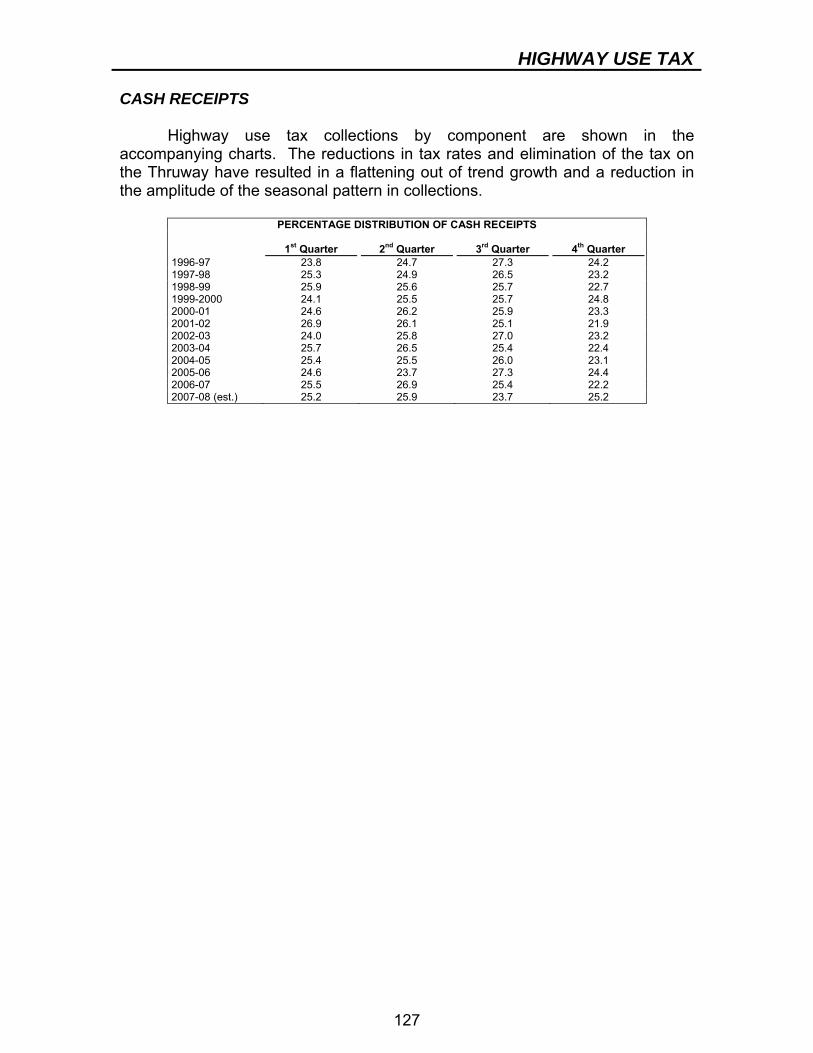
HIGHWAY USE TAX
127
CASH RECEIPTS Highway use tax collections by component are shown in the accompanying charts. The reductions in tax rates and elimination of the tax on the Thruway have resulted in a flattening out of trend growth and a reduction in the amplitude of the seasonal pattern in collections.
PERCENTAGE DISTRIBUTION OF CASH RECEIPTS 1st Quarter 2nd Quarter 3rd Quarter 4th Quarter 1996-97 23.8 24.7 27.3 24.2 1997-98 25.3 24.9 26.5 23.2 1998-99 25.9 25.6 25.7 22.7 1999-2000 24.1 25.5 25.7 24.8 2000-01 24.6 26.2 25.9 23.3 2001-02 26.9 26.1 25.1 21.9 2002-03 24.0 25.8 27.0 23.2 2003-04 25.7 26.5 25.4 22.4 2004-05 25.4 25.5 26.0 23.1 2005-06 24.6 23.7 27.3 24.4 2006-07 25.5 26.9 25.4 22.2 2007-08 (est.) 25.2 25.9 23.7 25.2
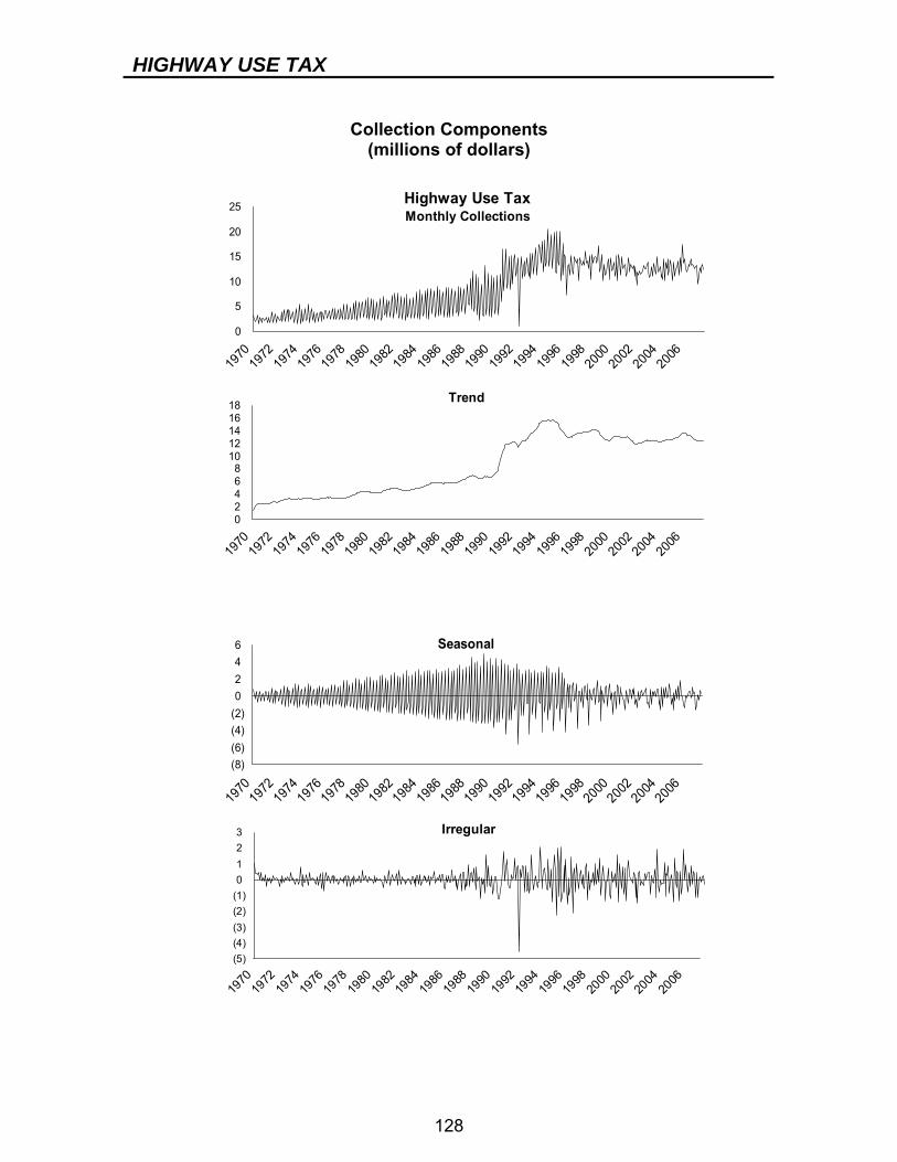
HIGHWAY USE TAX
128
Collection Components
(millions of dollars)
0
5
10
15
20
25
1970
1972
1974
1976
1978
1980
1982
1984
1986
1988
1990
1992
1994
1996
1998
2000
2002
2004
2006
Highway Use TaxMonthly Collections
02468
1012141618
1970
1972
1974
1976
1978
1980
1982
1984
1986
1988
1990
1992
1994
1996
1998
2000
2002
2004
2006
Trend
(8)(6)(4)(2)0246
1970
1972
1974
1976
1978
1980
1982
1984
1986
1988
1990
1992
1994
1996
1998
2000
2002
2004
2006
Seasonal
(5)(4)(3)(2)(1)0123
1970
1972
1974
1976
1978
1980
1982
1984
1986
1988
1990
1992
1994
1996
1998
2000
2002
2004
2006
Irregular
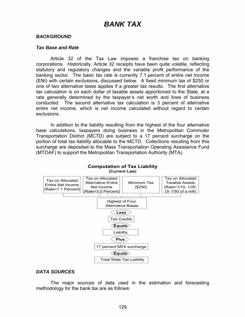
129
BANK TAX BACKGROUND Tax Base and Rate Article 32 of the Tax Law imposes a franchise tax on banking corporations. Historically, Article 32 receipts have been quite volatile, reflecting statutory and regulatory changes and the variable profit performance of the banking sector. The basic tax rate is currently 7.1 percent of entire net income (ENI) with certain exclusions, discussed below. A fixed minimum tax of $250 or one of two alternative taxes applies if a greater tax results. The first alternative tax calculation is on each dollar of taxable assets apportioned to the State, at a rate generally determined by the taxpayer’s net worth and lines of business conducted. The second alternative tax calculation is 3 percent of alternative entire net income, which is net income calculated without regard to certain exclusions. In addition to the liability resulting from the highest of the four alternative base calculations, taxpayers doing business in the Metropolitan Commuter Transportation District (MCTD) are subject to a 17 percent surcharge on the portion of total tax liability allocable to the MCTD. Collections resulting from this surcharge are deposited to the Mass Transportation Operating Assistance Fund (MTOAF) to support the Metropolitan Transportation Authority (MTA).
Tax on AllocatedEntire Net Income(Rate=7.1 Percent)
Tax on AllocatedTaxable Assets
(Rate=1/10, 1/25,Or 1/50 of a mill)
Minimum Tax($250)
Tax on AllocatedAlternative Entire
Net Income(Rate=3.0 Percent)
Highest of Four Alternative Bases
Tax Credits
Liability
17 percent MTA surcharge
Less
Equals
Computation of Tax Liability(Current Law)
Plus
EqualsTotal State Tax Liability
DATA SOURCES The major sources of data used in the estimation and forecasting methodology for the bank tax are as follows:
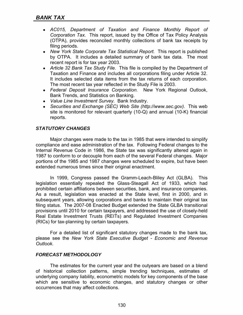
BANK TAX
130
● AC015, Department of Taxation and Finance Monthly Report of Corporation Tax. This report, issued by the Office of Tax Policy Analysis (OTPA), provides reconciled monthly collections of bank tax receipts by filing periods.
● New York State Corporate Tax Statistical Report. This report is published by OTPA. It includes a detailed summary of bank tax data. The most recent report is for tax year 2003.
● Article 32 Bank Tax Study File. This file is compiled by the Department of Taxation and Finance and includes all corporations filing under Article 32. It includes selected data items from the tax returns of each corporation. The most recent tax year reflected in the Study File is 2003.
● Federal Deposit Insurance Corporation. New York Regional Outlook, Bank Trends, and Statistics on Banking.
● Value Line Investment Survey. Bank Industry. ● Securities and Exchange (SEC) Web Site (http://www.sec.gov). This web
site is monitored for relevant quarterly (10-Q) and annual (10-K) financial reports.
STATUTORY CHANGES Major changes were made to the tax in 1985 that were intended to simplify compliance and ease administration of the tax. Following Federal changes to the Internal Revenue Code in 1986, the State tax was significantly altered again in 1987 to conform to or decouple from each of the several Federal changes. Major portions of the 1985 and 1987 changes were scheduled to expire, but have been extended numerous times since their original enactment. In 1999, Congress passed the Gramm-Leach-Bliley Act (GLBA). This legislation essentially repealed the Glass-Steagall Act of 1933, which had prohibited certain affiliations between securities, bank, and insurance companies. As a result, legislation was enacted at the State level, first in 2000, and in subsequent years, allowing corporations and banks to maintain their original tax filing status. The 2007-08 Enacted Budget extended the State GLBA transitional provisions until 2010 for certain taxpayers, and addressed the use of closely-held Real Estate Investment Trusts (REITs) and Regulated Investment Companies (RICs) for tax-planning by certain taxpayers. For a detailed list of significant statutory changes made to the bank tax, please see the New York State Executive Budget - Economic and Revenue Outlook. FORECAST METHODOLOGY The estimates for the current year and the outyears are based on a blend of historical collection patterns, simple trending techniques, estimates of underlying company liability, econometric models for key components of the base which are sensitive to economic changes, and statutory changes or other occurrences that may affect collections.
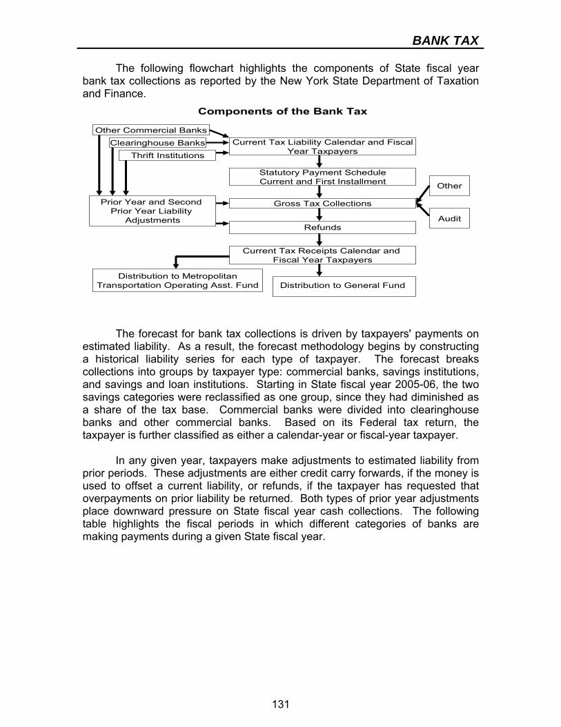
BANK TAX
131
The following flowchart highlights the components of State fiscal year bank tax collections as reported by the New York State Department of Taxation and Finance.
Components of the Bank Tax
Current Tax Liability Calendar and FiscalYear Taxpayers
Distribution to MetropolitanTransportation Operating Asst. Fund
Statutory Payment ScheduleCurrent and First Installment
Gross Tax Collections
Refunds
Current Tax Receipts Calendar and Fiscal Year Taxpayers
Prior Year and Second Prior Year Liability
Adjustments
Thrift Institutions
Other Commercial Banks
Other
Audit
Distribution to General Fund
Clearinghouse Banks
The forecast for bank tax collections is driven by taxpayers' payments on estimated liability. As a result, the forecast methodology begins by constructing a historical liability series for each type of taxpayer. The forecast breaks collections into groups by taxpayer type: commercial banks, savings institutions, and savings and loan institutions. Starting in State fiscal year 2005-06, the two savings categories were reclassified as one group, since they had diminished as a share of the tax base. Commercial banks were divided into clearinghouse banks and other commercial banks. Based on its Federal tax return, the taxpayer is further classified as either a calendar-year or fiscal-year taxpayer. In any given year, taxpayers make adjustments to estimated liability from prior periods. These adjustments are either credit carry forwards, if the money is used to offset a current liability, or refunds, if the taxpayer has requested that overpayments on prior liability be returned. Both types of prior year adjustments place downward pressure on State fiscal year cash collections. The following table highlights the fiscal periods in which different categories of banks are making payments during a given State fiscal year.
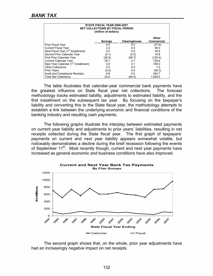
BANK TAX
132
STATE FISCAL YEAR 2006-2007 NET COLLECTIONS BY FISCAL PERIOD
(million of dollars)
Other Savings Clearinghouse Commercial Prior Fiscal Year 0.4 0.0 (37.9) Current Fiscal Year 2.3 0.0 48.3 Next Fiscal Year (1st Installment) 2.0 0.0 35.9 Second Prior Calendar Year (0.1) (2.0) 14.8 First Prior Calendar Year (26.5) (65.7) (125.4) Current Calendar Year 35.7 2.7 728.8 Next Year Calendar (1st Installment) 4.5 4.1 185.0 Other Collections 0.0 0.0 1.5 Prior Years (0.2) 0.5 (36.3) Audit and Compliance Receipts 6.8 0.0 244.7 Total Net Collections 24.9 (60.5) 1,059.5
The table illustrates that calendar-year commercial bank payments have the greatest influence on State fiscal year net collections. The forecast methodology tracks estimated liability, adjustments to estimated liability, and the first installment on the subsequent tax year. By focusing on the taxpayer’s liability and converting this to the State fiscal year, the methodology attempts to establish a link between the underlying economic and financial conditions of the banking industry and resulting cash payments. The following graphs illustrate the interplay between estimated payments on current year liability and adjustments to prior years’ liabilities, resulting in net receipts collected during the State fiscal year. The first graph of taxpayers’ payments on current and next year liability appears somewhat volatile, but noticeably demonstrates a decline during the brief recession following the events of September 11th. Most recently though, current and next year payments have increased as general economic and business conditions have also improved.
Current and Next Year Bank Tax Payments By Filer Groups
0
200
400
600
800
1000
1200
1994
1995
1996
1997
1998
1999
2000
2001
2002
2003
2004
2005
2006
2007
State Fiscal Year Ending
$ in
Mill
ions
Calendar Fiscal
The second graph shows that, on the whole, prior year adjustments have had an increasingly negative impact on net receipts.
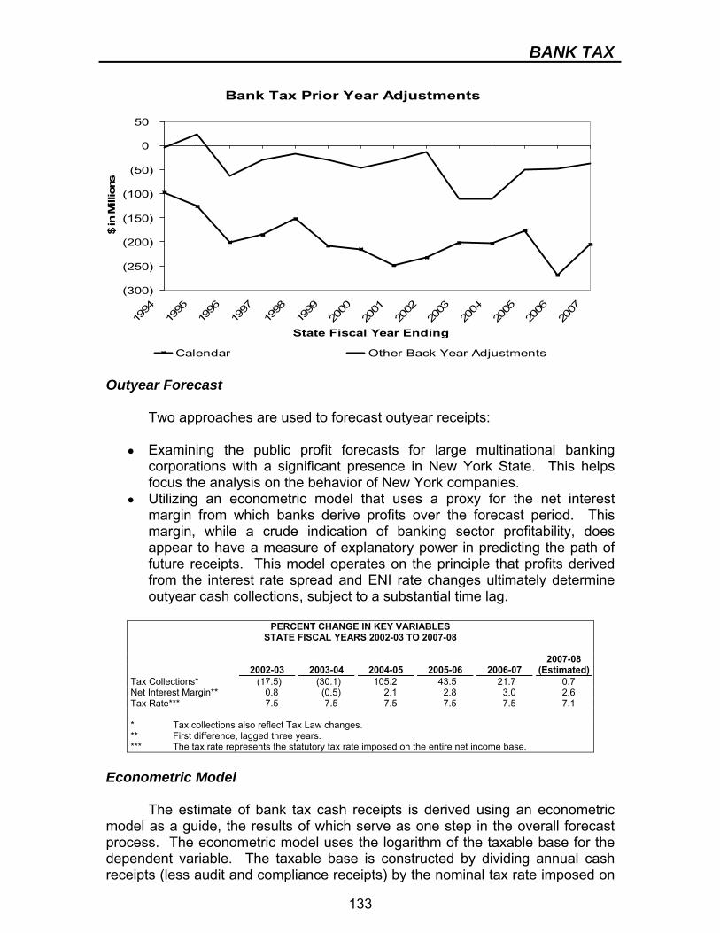
BANK TAX
133
Bank Tax Prior Year Adjustments
(300)
(250)
(200)
(150)
(100)
(50)
0
50
1994
1995
1996
1997
1998
1999
2000
2001
2002
2003
2004
2005
2006
2007
State Fiscal Year Ending
$ in
Mill
ions
Calendar Other Back Year Adjustments Outyear Forecast Two approaches are used to forecast outyear receipts:
● Examining the public profit forecasts for large multinational banking corporations with a significant presence in New York State. This helps focus the analysis on the behavior of New York companies.
● Utilizing an econometric model that uses a proxy for the net interest margin from which banks derive profits over the forecast period. This margin, while a crude indication of banking sector profitability, does appear to have a measure of explanatory power in predicting the path of future receipts. This model operates on the principle that profits derived from the interest rate spread and ENI rate changes ultimately determine outyear cash collections, subject to a substantial time lag.
PERCENT CHANGE IN KEY VARIABLES
STATE FISCAL YEARS 2002-03 TO 2007-08
2007-08 2002-03 2003-04 2004-05 2005-06 2006-07 (Estimated)Tax Collections* (17.5) (30.1) 105.2 43.5 21.7 0.7 Net Interest Margin** 0.8 (0.5) 2.1 2.8 3.0 2.6 Tax Rate*** 7.5 7.5 7.5 7.5 7.5 7.1 * Tax collections also reflect Tax Law changes. ** First difference, lagged three years. *** The tax rate represents the statutory tax rate imposed on the entire net income base.
Econometric Model The estimate of bank tax cash receipts is derived using an econometric model as a guide, the results of which serve as one step in the overall forecast process. The econometric model uses the logarithm of the taxable base for the dependent variable. The taxable base is constructed by dividing annual cash receipts (less audit and compliance receipts) by the nominal tax rate imposed on
BANK TAX
134
the ENI base for that year. Utilization of this method provides historical values for the dependent variable that exhibit a stronger correlation to the model regressors through time, as they are free of exogenous tax rate effects. The estimated bank tax base is then multiplied by the current law nominal tax rate on the ENI base to provide a baseline, net bank tax cash receipts estimate. Dependent Variable
● The logarithm of the taxable bank tax base, calculated as described above.
Net Interest Margin.
● The spread between the 10-year U.S. Treasury rate and the effective Federal Funds rate, lagged three years (12 quarters).
Bank Base
● Net bank tax collections divided by that year’s nominal ENI tax rate, converted to logs and lagged one full year (four quarters). This attempts to capture the effect of the cyclical element of the bank tax payment structure on future cash collections.
Dq2
● A dummy variable to account for seasonality with respect to second quarter collections.
Bank Rate
● The nominal bank tax rate applied to the ENI base for a given period, currently 7.1 percent. The ENI base is the base under which the majority of tax liability is incurred.
The Durbin-Watson statistic at a 95 percent confidence interval results in a failure to reject the null hypothesis that there is no significant serial correlation. The model implies a long-run elasticity with respect to the net interest margin of about 0.17.
BANK TAX CASH RECEIPTS MODEL Log(Bank Base t) = 3.007 - 0.269 * log(Bank Base t-4) + 0.363 * (Dq2) + 0.216 * log(Net Interest Margin t-12) + errort (7.32) (-1.70) (2.96) (4.09) Net Bank Tax Cash Receiptst = Bank Base t * Bank Rate ( 0.071) R-Bar Squared 0.4438 Durbin-Watson Statistic 1.8559 Root Mean Squared Error 0.3430 Number of Observations 43
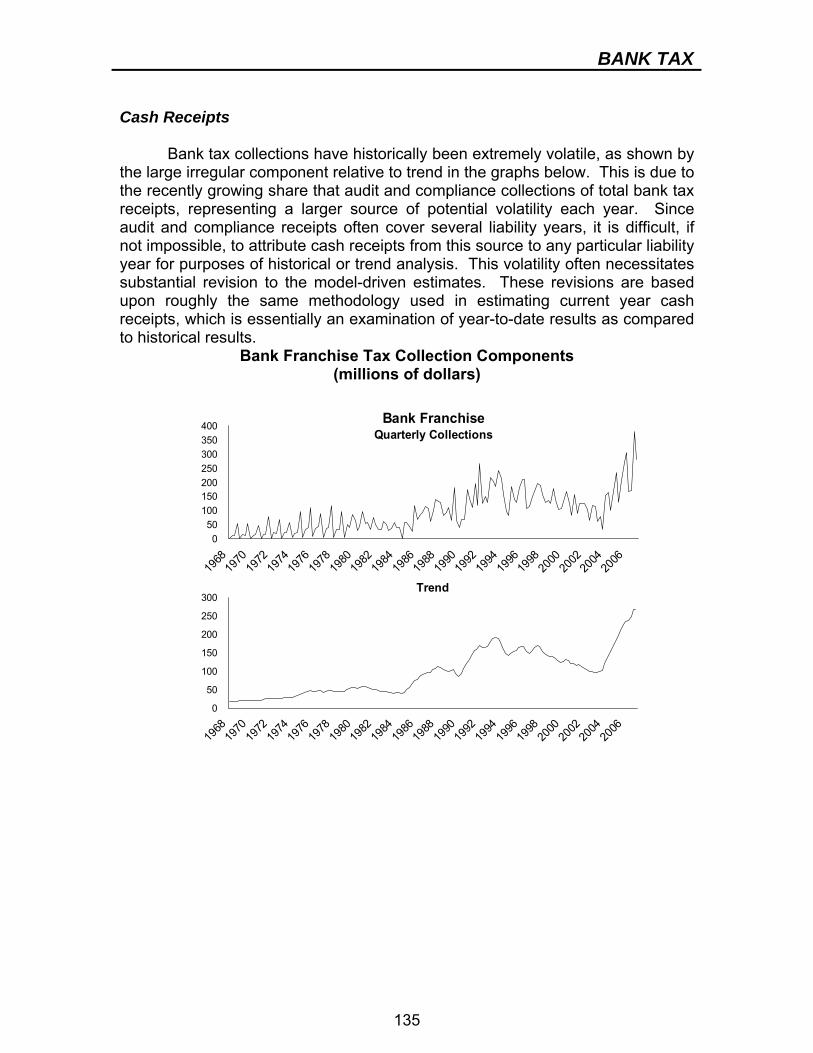
BANK TAX
135
Cash Receipts Bank tax collections have historically been extremely volatile, as shown by the large irregular component relative to trend in the graphs below. This is due to the recently growing share that audit and compliance collections of total bank tax receipts, representing a larger source of potential volatility each year. Since audit and compliance receipts often cover several liability years, it is difficult, if not impossible, to attribute cash receipts from this source to any particular liability year for purposes of historical or trend analysis. This volatility often necessitates substantial revision to the model-driven estimates. These revisions are based upon roughly the same methodology used in estimating current year cash receipts, which is essentially an examination of year-to-date results as compared to historical results.
Bank Franchise Tax Collection Components (millions of dollars)
050
100150200250300350400
1968
1970
1972
1974
1976
1978
1980
1982
1984
1986
1988
1990
1992
1994
1996
1998
2000
2002
2004
2006
Bank FranchiseQuarterly Collections
0
50
100
150
200
250
300
1968
1970
1972
1974
1976
1978
1980
1982
1984
1986
1988
1990
1992
1994
1996
1998
2000
2002
2004
2006
Trend
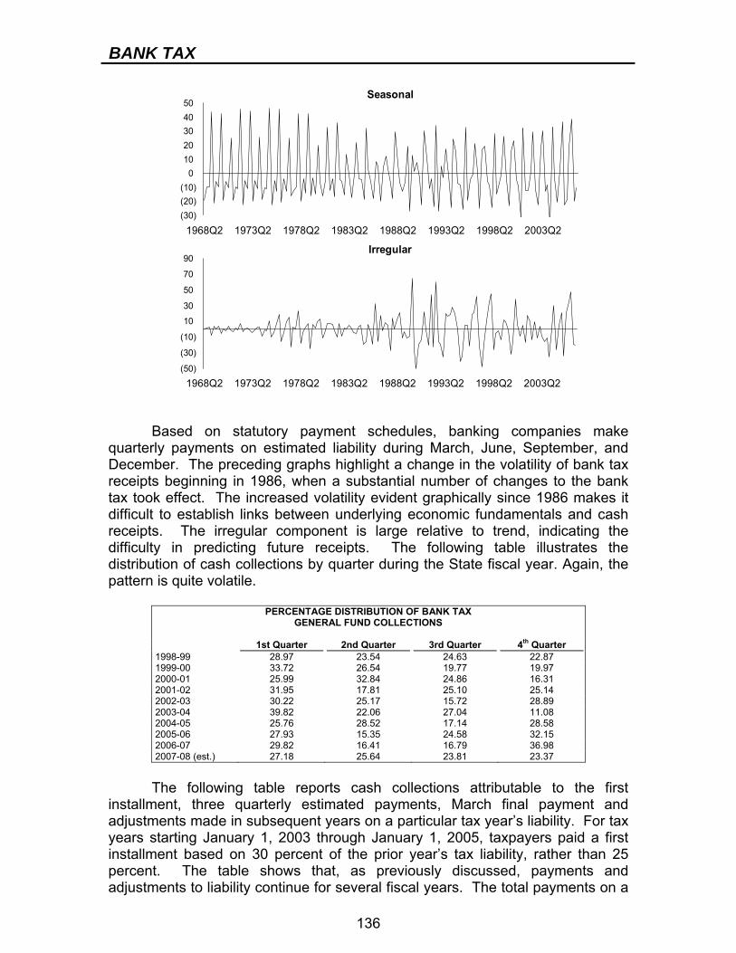
BANK TAX
136
(30)(20)(10)
01020304050
1968Q2 1973Q2 1978Q2 1983Q2 1988Q2 1993Q2 1998Q2 2003Q2
Seasonal
(50)
(30)
(10)
10
30
50
70
90
1968Q2 1973Q2 1978Q2 1983Q2 1988Q2 1993Q2 1998Q2 2003Q2
Irregular
Based on statutory payment schedules, banking companies make quarterly payments on estimated liability during March, June, September, and December. The preceding graphs highlight a change in the volatility of bank tax receipts beginning in 1986, when a substantial number of changes to the bank tax took effect. The increased volatility evident graphically since 1986 makes it difficult to establish links between underlying economic fundamentals and cash receipts. The irregular component is large relative to trend, indicating the difficulty in predicting future receipts. The following table illustrates the distribution of cash collections by quarter during the State fiscal year. Again, the pattern is quite volatile.
PERCENTAGE DISTRIBUTION OF BANK TAX GENERAL FUND COLLECTIONS
1st Quarter 2nd Quarter 3rd Quarter 4th Quarter 1998-99 28.97 23.54 24.63 22.87 1999-00 33.72 26.54 19.77 19.97 2000-01 25.99 32.84 24.86 16.31 2001-02 31.95 17.81 25.10 25.14 2002-03 30.22 25.17 15.72 28.89 2003-04 39.82 22.06 27.04 11.08 2004-05 25.76 28.52 17.14 28.58 2005-06 27.93 15.35 24.58 32.15 2006-07 29.82 16.41 16.79 36.98 2007-08 (est.) 27.18 25.64 23.81 23.37
The following table reports cash collections attributable to the first installment, three quarterly estimated payments, March final payment and adjustments made in subsequent years on a particular tax year’s liability. For tax years starting January 1, 2003 through January 1, 2005, taxpayers paid a first installment based on 30 percent of the prior year’s tax liability, rather than 25 percent. The table shows that, as previously discussed, payments and adjustments to liability continue for several fiscal years. The total payments on a
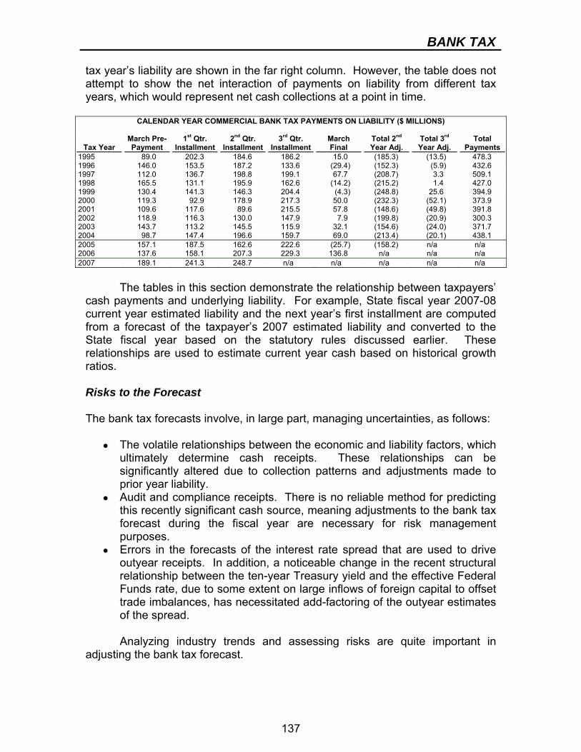
BANK TAX
137
tax year’s liability are shown in the far right column. However, the table does not attempt to show the net interaction of payments on liability from different tax years, which would represent net cash collections at a point in time.
CALENDAR YEAR COMMERCIAL BANK TAX PAYMENTS ON LIABILITY ($ MILLIONS)
Tax Year
March Pre- Payment
1st Qtr. Installment
2nd Qtr. Installment
3rd Qtr. Installment
March Final
Total 2nd
Year Adj. Total 3rd
Year Adj. Total
Payments 1995 89.0 202.3 184.6 186.2 15.0 (185.3) (13.5) 478.3 1996 146.0 153.5 187.2 133.6 (29.4) (152.3) (5.9) 432.6 1997 112.0 136.7 198.8 199.1 67.7 (208.7) 3.3 509.1 1998 165.5 131.1 195.9 162.6 (14.2) (215.2) 1.4 427.0 1999 130.4 141.3 146.3 204.4 (4.3) (248.8) 25.6 394.9 2000 119.3 92.9 178.9 217.3 50.0 (232.3) (52.1) 373.9 2001 109.6 117.6 89.6 215.5 57.8 (148.6) (49.8) 391.8 2002 118.9 116.3 130.0 147.9 7.9 (199.8) (20.9) 300.3 2003 143.7 113.2 145.5 115.9 32.1 (154.6) (24.0) 371.7 2004 98.7 147.4 196.6 159.7 69.0 (213.4) (20.1) 438.1 2005 157.1 187.5 162.6 222.6 (25.7) (158.2) n/a n/a 2006 137.6 158.1 207.3 229.3 136.8 n/a n/a n/a 2007 189.1 241.3 248.7 n/a n/a n/a n/a n/a
The tables in this section demonstrate the relationship between taxpayers’ cash payments and underlying liability. For example, State fiscal year 2007-08 current year estimated liability and the next year’s first installment are computed from a forecast of the taxpayer’s 2007 estimated liability and converted to the State fiscal year based on the statutory rules discussed earlier. These relationships are used to estimate current year cash based on historical growth ratios. Risks to the Forecast The bank tax forecasts involve, in large part, managing uncertainties, as follows:
● The volatile relationships between the economic and liability factors, which ultimately determine cash receipts. These relationships can be significantly altered due to collection patterns and adjustments made to prior year liability.
● Audit and compliance receipts. There is no reliable method for predicting this recently significant cash source, meaning adjustments to the bank tax forecast during the fiscal year are necessary for risk management purposes.
● Errors in the forecasts of the interest rate spread that are used to drive outyear receipts. In addition, a noticeable change in the recent structural relationship between the ten-year Treasury yield and the effective Federal Funds rate, due to some extent on large inflows of foreign capital to offset trade imbalances, has necessitated add-factoring of the outyear estimates of the spread.
Analyzing industry trends and assessing risks are quite important in adjusting the bank tax forecast.
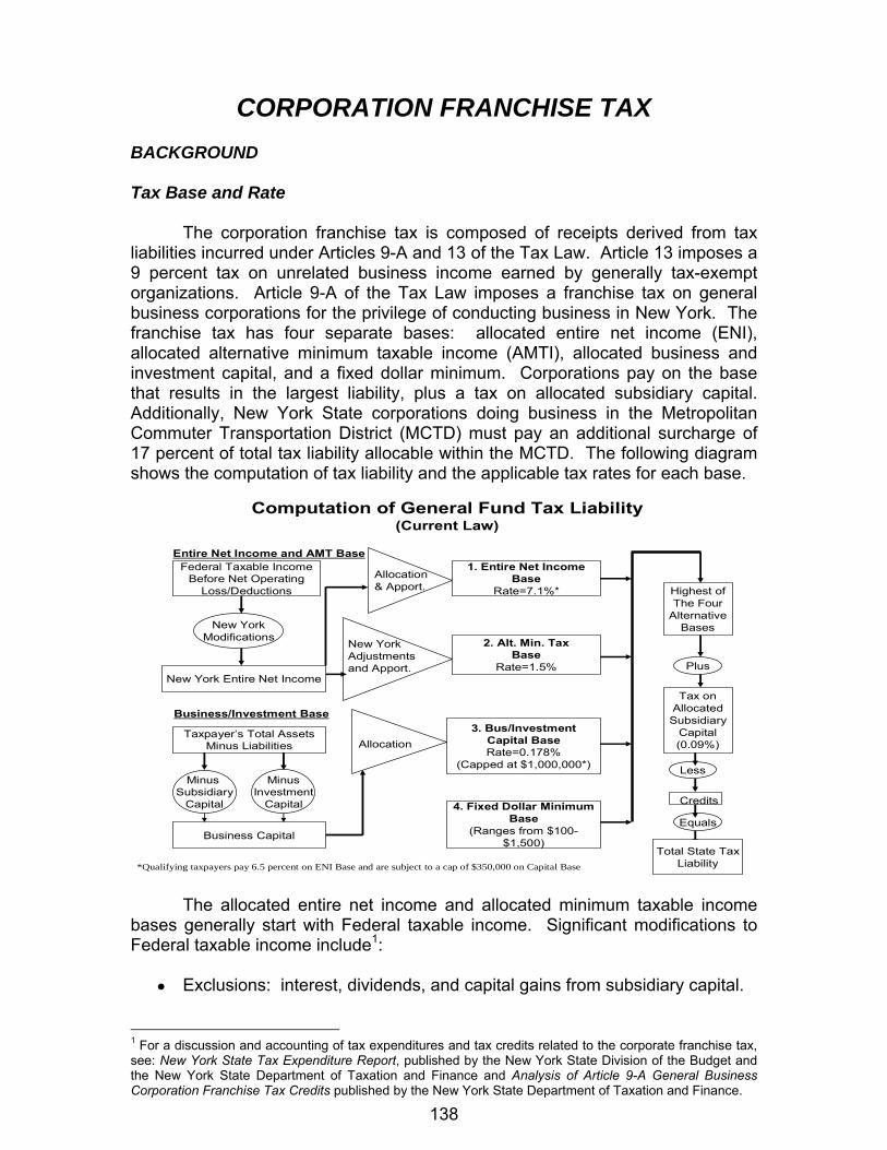
138
CORPORATION FRANCHISE TAX
BACKGROUND Tax Base and Rate The corporation franchise tax is composed of receipts derived from tax liabilities incurred under Articles 9-A and 13 of the Tax Law. Article 13 imposes a 9 percent tax on unrelated business income earned by generally tax-exempt organizations. Article 9-A of the Tax Law imposes a franchise tax on general business corporations for the privilege of conducting business in New York. The franchise tax has four separate bases: allocated entire net income (ENI), allocated alternative minimum taxable income (AMTI), allocated business and investment capital, and a fixed dollar minimum. Corporations pay on the base that results in the largest liability, plus a tax on allocated subsidiary capital. Additionally, New York State corporations doing business in the Metropolitan Commuter Transportation District (MCTD) must pay an additional surcharge of 17 percent of total tax liability allocable within the MCTD. The following diagram shows the computation of tax liability and the applicable tax rates for each base.
Federal Taxable IncomeBefore Net Operating
Loss/Deductions
Entire Net Income and AMT Base
New YorkModifications
New York Entire Net Income
1. Entire Net IncomeBase
Rate=7.1%*
2. Alt. Min. TaxBase
Rate=1.5%
Allocation& Apport.
New York Adjustments and Apport.
Business/Investment Base
AllocationTaxpayer’s Total Assets
Minus Liabilities
Minus Subsidiary
Capital
MinusInvestment
Capital
Business Capital
3. Bus/InvestmentCapital BaseRate=0.178%
(Capped at $1,000,000*)
4. Fixed Dollar MinimumBase
(Ranges from $100-$1,500)
Highest ofThe Four
AlternativeBases
Plus
Tax onAllocatedSubsidiary
Capital(0.09%)
Less
Equals
Credits
Total State TaxLiability
Computation of General Fund Tax Liability(Current Law)
*Qualifying taxpayers pay 6.5 percent on ENI Base and are subject to a cap of $350,000 on Capital Base
The allocated entire net income and allocated minimum taxable income bases generally start with Federal taxable income. Significant modifications to Federal taxable income include1:
● Exclusions: interest, dividends, and capital gains from subsidiary capital.
1 For a discussion and accounting of tax expenditures and tax credits related to the corporate franchise tax, see: New York State Tax Expenditure Report, published by the New York State Division of the Budget and the New York State Department of Taxation and Finance and Analysis of Article 9-A General Business Corporation Franchise Tax Credits published by the New York State Department of Taxation and Finance.
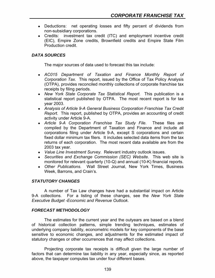
CORPORATE FRANCHISE TAX
139
● Deductions: net operating losses and fifty percent of dividends from non-subsidiary corporations.
● Credits: investment tax credit (ITC) and employment incentive credit (EIC), Empire Zone credits, Brownfield credits and Empire State Film Production credit.
DATA SOURCES The major sources of data used to forecast this tax include:
● AC015 Department of Taxation and Finance Monthly Report of Corporation Tax. This report, issued by the Office of Tax Policy Analysis (OTPA), provides reconciled monthly collections of corporate franchise tax receipts by filing periods.
● New York State Corporate Tax Statistical Report. This publication is a statistical report published by OTPA. The most recent report is for tax year 2003.
● Analysis of Article 9-A General Business Corporation Franchise Tax Credit Report. This report, published by OTPA, provides an accounting of credit activity under Article 9-A.
● Article 9-A Corporation Franchise Tax Study File. These files are compiled by the Department of Taxation and Finance and include all corporations filing under Article 9-A, except S corporations and certain fixed dollar minimum tax filers. It includes selected data items from the tax returns of each corporation. The most recent data available are from the 2003 tax year.
● Value Line Investment Survey. Relevant industry outlook issues. ● Securities and Exchange Commission (SEC) Website. This web site is
monitored for relevant quarterly (10-Q) and annual (10-K) financial reports. ● Other Publications. Wall Street Journal, New York Times, Business
Week, Barrons, and Crain’s. STATUTORY CHANGES A number of Tax Law changes have had a substantial impact on Article 9-A collections. For a listing of these changes, see the New York State Executive Budget -Economic and Revenue Outlook. FORECAST METHODOLOGY The estimates for the current year and the outyears are based on a blend of historical collection patterns, simple trending techniques, estimates of underlying company liability, econometric models for key components of the base sensitive to economic changes, and adjustments for the estimated impact of statutory changes or other occurrences that may affect collections. Projecting corporate tax receipts is difficult given the large number of factors that can determine tax liability in any year, especially since, as reported above, the taxpayer computes tax under four different bases.
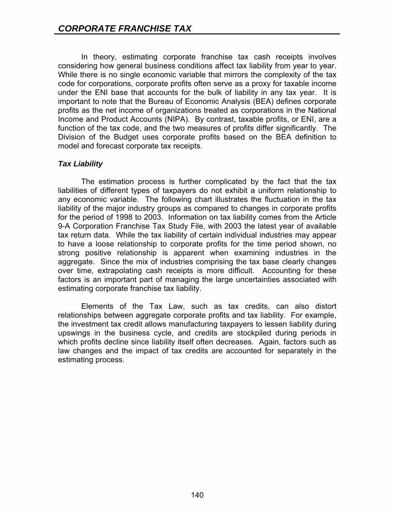
CORPORATE FRANCHISE TAX
140
In theory, estimating corporate franchise tax cash receipts involves considering how general business conditions affect tax liability from year to year. While there is no single economic variable that mirrors the complexity of the tax code for corporations, corporate profits often serve as a proxy for taxable income under the ENI base that accounts for the bulk of liability in any tax year. It is important to note that the Bureau of Economic Analysis (BEA) defines corporate profits as the net income of organizations treated as corporations in the National Income and Product Accounts (NIPA). By contrast, taxable profits, or ENI, are a function of the tax code, and the two measures of profits differ significantly. The Division of the Budget uses corporate profits based on the BEA definition to model and forecast corporate tax receipts. Tax Liability The estimation process is further complicated by the fact that the tax liabilities of different types of taxpayers do not exhibit a uniform relationship to any economic variable. The following chart illustrates the fluctuation in the tax liability of the major industry groups as compared to changes in corporate profits for the period of 1998 to 2003. Information on tax liability comes from the Article 9-A Corporation Franchise Tax Study File, with 2003 the latest year of available tax return data. While the tax liability of certain individual industries may appear to have a loose relationship to corporate profits for the time period shown, no strong positive relationship is apparent when examining industries in the aggregate. Since the mix of industries comprising the tax base clearly changes over time, extrapolating cash receipts is more difficult. Accounting for these factors is an important part of managing the large uncertainties associated with estimating corporate franchise tax liability. Elements of the Tax Law, such as tax credits, can also distort relationships between aggregate corporate profits and tax liability. For example, the investment tax credit allows manufacturing taxpayers to lessen liability during upswings in the business cycle, and credits are stockpiled during periods in which profits decline since liability itself often decreases. Again, factors such as law changes and the impact of tax credits are accounted for separately in the estimating process.
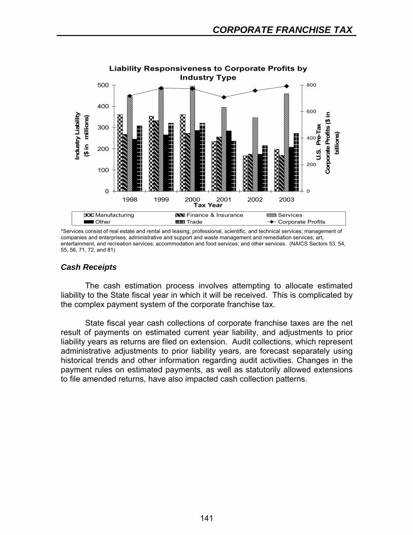
CORPORATE FRANCHISE TAX
141
Liability Responsiveness to Corporate Profits by Industry Type
0
100
200
300
400
500
1998 1999 2000 2001 2002 2003Tax Year
Indu
stry
Lia
bilit
y ($
in
mill
ions
)
0
200
400
600
800
U.S
. Pr
e-Ta
x C
orpo
rate
Pro
fits
($ in
bi
llion
s)
Manufacturing Finance & Insurance ServicesOther Trade Corporate Profits
*Services consist of real estate and rental and leasing; professional, scientific, and technical services; management of companies and enterprises; administrative and support and waste management and remediation services; art, entertainment, and recreation services; accommodation and food services; and other services. (NAICS Sectors 53, 54, 55, 56, 71, 72, and 81) Cash Receipts The cash estimation process involves attempting to allocate estimated liability to the State fiscal year in which it will be received. This is complicated by the complex payment system of the corporate franchise tax. State fiscal year cash collections of corporate franchise taxes are the net result of payments on estimated current year liability, and adjustments to prior liability years as returns are filed on extension. Audit collections, which represent administrative adjustments to prior liability years, are forecast separately using historical trends and other information regarding audit activities. Changes in the payment rules on estimated payments, as well as statutorily allowed extensions to file amended returns, have also impacted cash collection patterns.
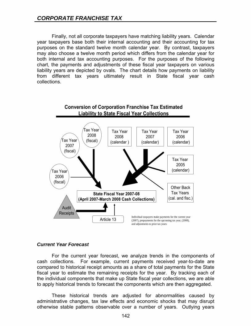
CORPORATE FRANCHISE TAX
142
Finally, not all corporate taxpayers have matching liability years. Calendar year taxpayers base both their internal accounting and their accounting for tax purposes on the standard twelve month calendar year. By contrast, taxpayers may also choose a twelve month period which differs from the calendar year for both internal and tax accounting purposes. For the purposes of the following chart, the payments and adjustments of these fiscal year taxpayers on various liability years are depicted by ovals. The chart details how payments on liability from different tax years ultimately result in State fiscal year cash collections.
Conversion of Corporation Franchise Tax Estimated Liability to State Fiscal Year Collections
Tax Year2006
(fiscal)
Tax Year2008
(calendar )
Tax Year 2007
(calendar)
Tax Year2006
(calendar)
Tax Year 2005
(calendar)
Other BackTax Years
(cal. and fisc.)State Fiscal Year 2007-08
(April 2007-March 2008 Cash Collections)
AuditReceipts
Tax Year 2007
(fiscal)
Tax Year 2008
(fiscal)
Individual taxpayers make payments for the current year (2007), prepayments for the upcoming tax year, (2008), and adjustments to prior tax years
Article 13
Current Year Forecast For the current year forecast, we analyze trends in the components of cash collections. For example, current payments received year-to-date are compared to historical receipt amounts as a share of total payments for the State fiscal year to estimate the remaining receipts for the year. By tracking each of the individual components that make up State fiscal year collections, we are able to apply historical trends to forecast the components which are then aggregated. These historical trends are adjusted for abnormalities caused by administrative changes, tax law effects and economic shocks that may disrupt otherwise stable patterns observable over a number of years. Outlying years
CORPORATE FRANCHISE TAX
143
may either be ignored entirely, or contrarily, extensive analysis may be performed in an attempt to uncover useful information that may continue to affect current results. The current forecasting methodology tracks the seven liability payment streams and the other unassigned liability payments (other back year calendar and audits and compliance receipts) indicated in the figure above to arrive at estimates of State fiscal year collections. Considerable attention has been given recently to the tracking and estimation of audit and compliance receipts. While nearly impossible to predict, survey information from the Department of Taxation and Finance allows us to continually adjust our estimate of audit and compliance receipts for the current year. The following two graphs illustrate the major payment streams analyzed within a State fiscal year (2nd prior calendar payments and other back year payments have been combined). The first graph shows the relatively stable upward trend in payments on current year estimated tax from calendar year tax payments. However, the second graph shows the large and somewhat erratic largely negative adjustments to cash based on prior year adjustments.
Article 9-A Current and Next Year Payments By Filer Groups
0.0
0.5
1.0
1.5
2.0
2.5
1981 1984 1987 1990 1993 1996 1999 2002 2005
State Fiscal Year Ending
$ in
Bill
ions
Fiscal Calendar
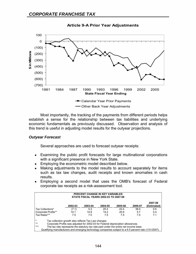
CORPORATE FRANCHISE TAX
144
Article 9-A Prior Year Adjustments
(700)
(600)
(500)
(400)
(300)
(200)
(100)
0
100
1981 1984 1987 1990 1993 1996 1999 2002 2005State Fiscal Year Ending
$ in
Mill
ions
Calendar Year Prior Payments
Other Back Year Adjustments Most importantly, the tracking of the payments from different periods helps establish a sense for the relationship between tax liabilities and underlying economic fundamentals as previously discussed. Observation and analysis of this trend is useful in adjusting model results for the outyear projections. Outyear Forecast Several approaches are used to forecast outyear receipts:
● Examining the public profit forecasts for large multinational corporations with a significant presence in New York State.
● Employing the econometric model described below. ● Making adjustments to the model results to account separately for items
such as tax law changes, audit receipts and known anomalies in cash results.
● Employing a second model that uses the OMB's forecast of Federal corporate tax receipts as a risk-assessment tool.
PERCENT CHANGE IN KEY VARIABLES
STATE FISCAL YEARS 2002-03 TO 2007-08
2007-08 2002-03 2003-04 2004-05 2005-06 2006-07 (Estimated)Tax Collections* (7.1) 5.3 25.4 43.4 38.0 0.6 Corporate Profits** 14.1 14.9 14.2 20.9 5.7 5.4 Tax Rates*** 7.5 7.5 7.5 7.5 7.5 7.1 * Tax collection growth also reflects Tax Law changes. ** Corporate Profits was adjusted for 2002-03 for Federal depreciation allowances. *** The tax rate represents the statutory tax rate paid under the entire net income base. Qualifying manufacturers and emerging technology companies subject to a 6.5 percent rate (1/31/2007).
CORPORATE FRANCHISE TAX
145
DOB Corporate Franchise Tax Cash Receipts Model The estimate of corporate franchise tax cash receipts is derived using an econometric model as a guide, the results of which serve as one part of the overall process. The econometric model relates gross corporate franchise tax collections to corporate profits, previous collection patterns and the nominal tax rate in effect at that time. Dependent Variable
● The logarithm of gross corporate franchise tax receipts, less audit and compliance receipts.
Corp. Prof.
● The logarithm of U.S. corporate profits, lagged one quarter. Gross 9-A
● The logarithm of gross corporate franchise tax collections, lagged a full year (four quarters). This attempts to capture the effect of the cyclical element of the corporate franchise tax payment structure on future cash collections.
9-A Rate
● The nominal corporate franchise tax rate applied to the ENI base for a given period, lagged one year (four quarters). The ENI base is the base under which the majority of tax liability is incurred. The recent reduction in the AMT rate, while potentially meaningful to individual taxpayers, does not significantly impact the liability of the tax base at-large.
d013
● A dummy variable that accounts for an anomaly in cash receipts in the third quarter of 2001. Cash collections were disrupted due to the events of September 11th, 2001.
dQ1
● A dummy variable that adjusts for the seasonality resulting from the typically larger first calendar year quarter (last State fiscal year quarter) cash receipts. Calendar year tax filers (which incur the majority of tax liability) typically report a portion of two tax liability years in this quarter. In March, both the final payment on the closing tax year's liability, as well as a pre-payment on the new tax year's liability, is due for these taxpayers. This seasonality is clearly demonstrated in the tables showing decomposition of the series later in this section.
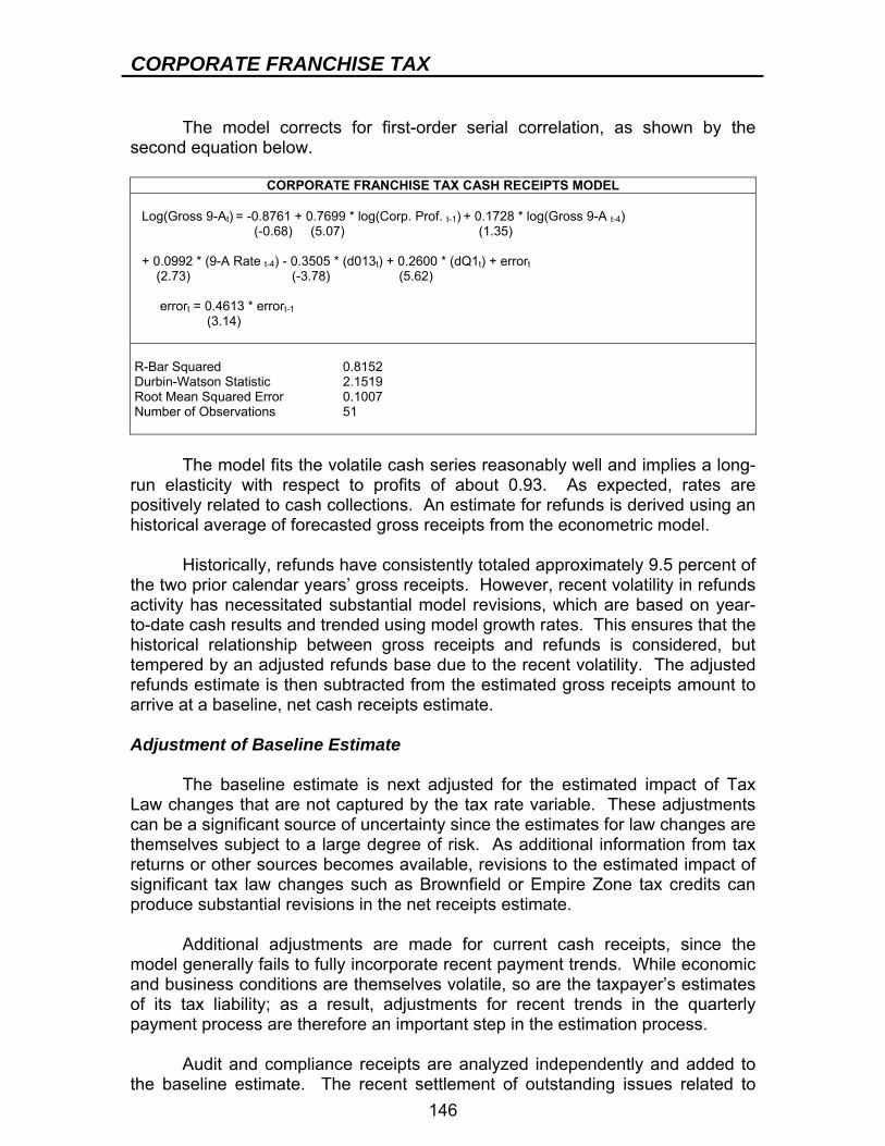
CORPORATE FRANCHISE TAX
146
The model corrects for first-order serial correlation, as shown by the second equation below.
CORPORATE FRANCHISE TAX CASH RECEIPTS MODEL Log(Gross 9-At) = -0.8761 + 0.7699 * log(Corp. Prof. t-1) + 0.1728 * log(Gross 9-A t-4) (-0.68) (5.07) (1.35) + 0.0992 * (9-A Rate t-4) - 0.3505 * (d013t) + 0.2600 * (dQ1t) + errort (2.73) (-3.78) (5.62) errort = 0.4613 * errort-1 (3.14) R-Bar Squared 0.8152 Durbin-Watson Statistic 2.1519 Root Mean Squared Error 0.1007 Number of Observations 51 The model fits the volatile cash series reasonably well and implies a long-run elasticity with respect to profits of about 0.93. As expected, rates are positively related to cash collections. An estimate for refunds is derived using an historical average of forecasted gross receipts from the econometric model. Historically, refunds have consistently totaled approximately 9.5 percent of the two prior calendar years’ gross receipts. However, recent volatility in refunds activity has necessitated substantial model revisions, which are based on year-to-date cash results and trended using model growth rates. This ensures that the historical relationship between gross receipts and refunds is considered, but tempered by an adjusted refunds base due to the recent volatility. The adjusted refunds estimate is then subtracted from the estimated gross receipts amount to arrive at a baseline, net cash receipts estimate. Adjustment of Baseline Estimate The baseline estimate is next adjusted for the estimated impact of Tax Law changes that are not captured by the tax rate variable. These adjustments can be a significant source of uncertainty since the estimates for law changes are themselves subject to a large degree of risk. As additional information from tax returns or other sources becomes available, revisions to the estimated impact of significant tax law changes such as Brownfield or Empire Zone tax credits can produce substantial revisions in the net receipts estimate. Additional adjustments are made for current cash receipts, since the model generally fails to fully incorporate recent payment trends. While economic and business conditions are themselves volatile, so are the taxpayer’s estimates of its tax liability; as a result, adjustments for recent trends in the quarterly payment process are therefore an important step in the estimation process. Audit and compliance receipts are analyzed independently and added to the baseline estimate. The recent settlement of outstanding issues related to
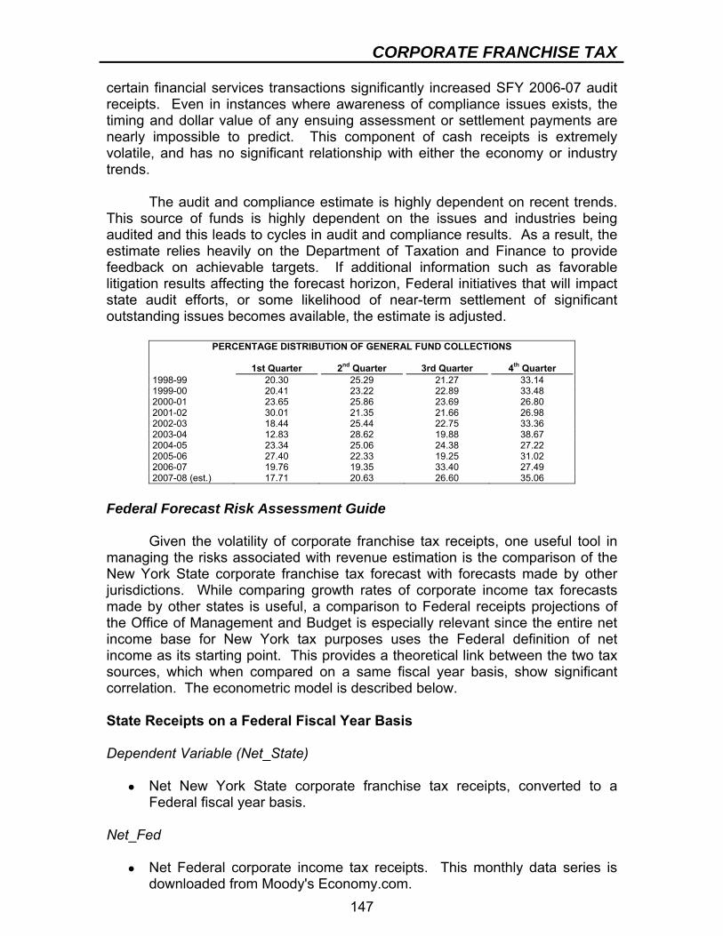
CORPORATE FRANCHISE TAX
147
certain financial services transactions significantly increased SFY 2006-07 audit receipts. Even in instances where awareness of compliance issues exists, the timing and dollar value of any ensuing assessment or settlement payments are nearly impossible to predict. This component of cash receipts is extremely volatile, and has no significant relationship with either the economy or industry trends. The audit and compliance estimate is highly dependent on recent trends. This source of funds is highly dependent on the issues and industries being audited and this leads to cycles in audit and compliance results. As a result, the estimate relies heavily on the Department of Taxation and Finance to provide feedback on achievable targets. If additional information such as favorable litigation results affecting the forecast horizon, Federal initiatives that will impact state audit efforts, or some likelihood of near-term settlement of significant outstanding issues becomes available, the estimate is adjusted.
PERCENTAGE DISTRIBUTION OF GENERAL FUND COLLECTIONS
1st Quarter 2nd Quarter 3rd Quarter 4th Quarter 1998-99 20.30 25.29 21.27 33.14 1999-00 20.41 23.22 22.89 33.48 2000-01 23.65 25.86 23.69 26.80 2001-02 30.01 21.35 21.66 26.98 2002-03 18.44 25.44 22.75 33.36 2003-04 12.83 28.62 19.88 38.67 2004-05 23.34 25.06 24.38 27.22 2005-06 27.40 22.33 19.25 31.02 2006-07 19.76 19.35 33.40 27.49 2007-08 (est.) 17.71 20.63 26.60 35.06
Federal Forecast Risk Assessment Guide Given the volatility of corporate franchise tax receipts, one useful tool in managing the risks associated with revenue estimation is the comparison of the New York State corporate franchise tax forecast with forecasts made by other jurisdictions. While comparing growth rates of corporate income tax forecasts made by other states is useful, a comparison to Federal receipts projections of the Office of Management and Budget is especially relevant since the entire net income base for New York tax purposes uses the Federal definition of net income as its starting point. This provides a theoretical link between the two tax sources, which when compared on a same fiscal year basis, show significant correlation. The econometric model is described below. State Receipts on a Federal Fiscal Year Basis Dependent Variable (Net_State)
● Net New York State corporate franchise tax receipts, converted to a Federal fiscal year basis.
Net_Fed
● Net Federal corporate income tax receipts. This monthly data series is downloaded from Moody's Economy.com.
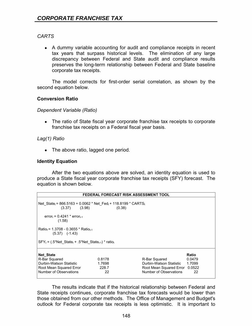
CORPORATE FRANCHISE TAX
148
CARTS
● A dummy variable accounting for audit and compliance receipts in recent tax years that surpass historical levels. The elimination of any large discrepancy between Federal and State audit and compliance results preserves the long-term relationship between Federal and State baseline corporate tax receipts.
The model corrects for first-order serial correlation, as shown by the second equation below. Conversion Ratio Dependent Variable (Ratio)
● The ratio of State fiscal year corporate franchise tax receipts to corporate franchise tax receipts on a Federal fiscal year basis.
Lag(1) Ratio
● The above ratio, lagged one period. Identity Equation After the two equations above are solved, an identity equation is used to produce a State fiscal year corporate franchise tax receipts (SFY) forecast. The equation is shown below.
FEDERAL FORECAST RISK ASSESSMENT TOOL Net_Statet = 866.5163 + 0.0062 * Net_Fedt + 118.8199 * CARTSt (3.37) (3.98) (0.38) errort = 0.4241 * errort-1 (1.58) Ratiot = 1.3708 - 0.3655 * Ratiot-1 (5.37) (-1.43) SFYt = (.5*Net_Statet + .5*Net_Statet-1) * ratiot Net_State Ratio R-Bar Squared 0.8178 R-Bar Squared 0.0479 Durbin-Watson Statistic 1.7698 Durbin-Watson Statistic 1.7099 Root Mean Squared Error 228.7 Root Mean Squared Error 0.0522 Number of Observations 22 Number of Observations 22 The results indicate that if the historical relationship between Federal and State receipts continues, corporate franchise tax forecasts would be lower than those obtained from our other methods. The Office of Management and Budget's outlook for Federal corporate tax receipts is less optimistic. It is important to
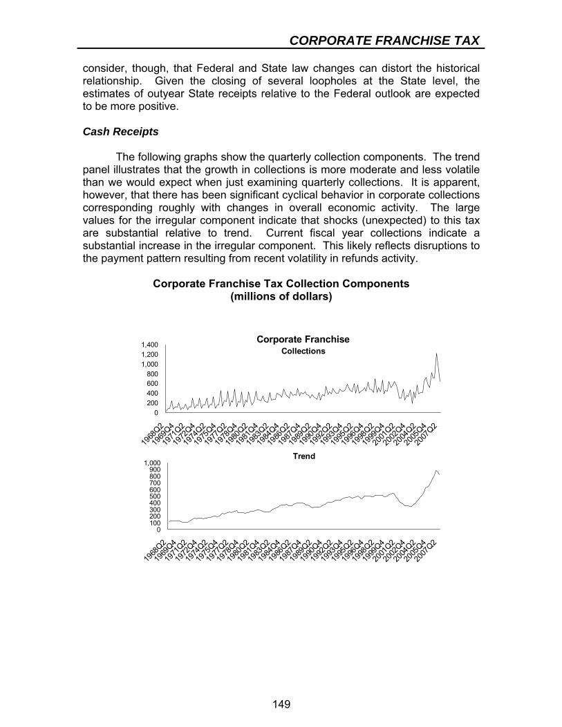
CORPORATE FRANCHISE TAX
149
consider, though, that Federal and State law changes can distort the historical relationship. Given the closing of several loopholes at the State level, the estimates of outyear State receipts relative to the Federal outlook are expected to be more positive. Cash Receipts The following graphs show the quarterly collection components. The trend panel illustrates that the growth in collections is more moderate and less volatile than we would expect when just examining quarterly collections. It is apparent, however, that there has been significant cyclical behavior in corporate collections corresponding roughly with changes in overall economic activity. The large values for the irregular component indicate that shocks (unexpected) to this tax are substantial relative to trend. Current fiscal year collections indicate a substantial increase in the irregular component. This likely reflects disruptions to the payment pattern resulting from recent volatility in refunds activity.
Corporate Franchise Tax Collection Components (millions of dollars)
0200400600800
1,0001,2001,400
1968
Q2
1969
Q4
1971
Q2
1972
Q4
1974
Q2
1975
Q4
1977
Q2
1978
Q4
1980
Q2
1981
Q4
1983
Q2
1984
Q4
1986
Q2
1987
Q4
1989
Q2
1990
Q4
1992
Q2
1993
Q4
1995
Q2
1996
Q4
1998
Q2
1999
Q4
2001
Q2
2002
Q4
2004
Q2
2005
Q4
2007
Q2
Corporate FranchiseCollections
0100200300400500600700800900
1,000
1968
Q2
1969
Q4
1971
Q2
1972
Q4
1974
Q2
1975
Q4
1977
Q2
1978
Q4
1980
Q2
1981
Q4
1983
Q2
1984
Q4
1986
Q2
1987
Q4
1989
Q2
1990
Q4
1992
Q2
1993
Q4
1995
Q2
1996
Q4
1998
Q2
1999
Q4
2001
Q2
2002
Q4
2004
Q2
2005
Q4
2007
Q2
Trend
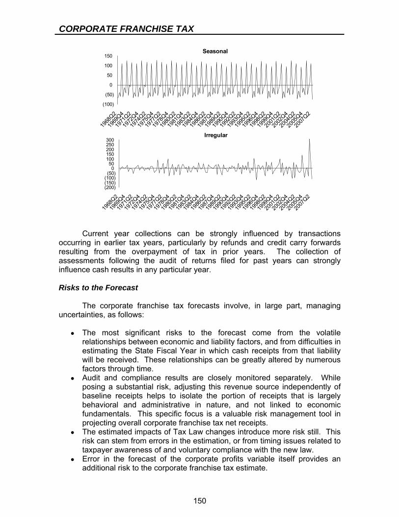
CORPORATE FRANCHISE TAX
150
(100)
(50)
0
50
100
150
1968
Q2
1969
Q4
1971
Q2
1972
Q4
1974
Q2
1975
Q4
1977
Q2
1978
Q4
1980
Q2
1981
Q4
1983
Q2
1984
Q4
1986
Q2
1987
Q4
1989
Q2
1990
Q4
1992
Q2
1993
Q4
1995
Q2
1996
Q4
1998
Q2
1999
Q4
2001
Q2
2002
Q4
2004
Q2
2005
Q4
2007
Q2
Seasonal
(200)(150)(100)(50)
050
100150200250300
1968
Q2
1969
Q4
1971
Q2
1972
Q4
1974
Q2
1975
Q4
1977
Q2
1978
Q4
1980
Q2
1981
Q4
1983
Q2
1984
Q4
1986
Q2
1987
Q4
1989
Q2
1990
Q4
1992
Q2
1993
Q4
1995
Q2
1996
Q4
1998
Q2
1999
Q4
2001
Q2
2002
Q4
2004
Q2
2005
Q4
2007
Q2
Irregular
Current year collections can be strongly influenced by transactions occurring in earlier tax years, particularly by refunds and credit carry forwards resulting from the overpayment of tax in prior years. The collection of assessments following the audit of returns filed for past years can strongly influence cash results in any particular year. Risks to the Forecast The corporate franchise tax forecasts involve, in large part, managing uncertainties, as follows:
● The most significant risks to the forecast come from the volatile relationships between economic and liability factors, and from difficulties in estimating the State Fiscal Year in which cash receipts from that liability will be received. These relationships can be greatly altered by numerous factors through time.
● Audit and compliance results are closely monitored separately. While posing a substantial risk, adjusting this revenue source independently of baseline receipts helps to isolate the portion of receipts that is largely behavioral and administrative in nature, and not linked to economic fundamentals. This specific focus is a valuable risk management tool in projecting overall corporate franchise tax net receipts.
● The estimated impacts of Tax Law changes introduce more risk still. This risk can stem from errors in the estimation, or from timing issues related to taxpayer awareness of and voluntary compliance with the new law.
● Error in the forecast of the corporate profits variable itself provides an additional risk to the corporate franchise tax estimate.

CORPORATE FRANCHISE TAX
151
As a result, analyzing industry trends, monitoring the forecasts of other tax jurisdictions, constantly reevaluating the impact of large tax expenditures, and balancing risks resulting from audit and compliance receipts are quite important in adjusting the Division of the Budget corporate franchise tax forecast.
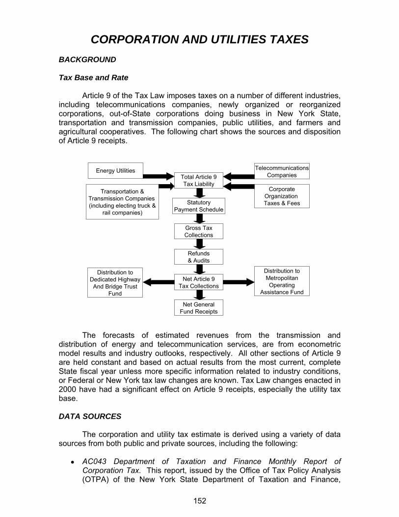
152
CORPORATION AND UTILITIES TAXES BACKGROUND Tax Base and Rate Article 9 of the Tax Law imposes taxes on a number of different industries, including telecommunications companies, newly organized or reorganized corporations, out-of-State corporations doing business in New York State, transportation and transmission companies, public utilities, and farmers and agricultural cooperatives. The following chart shows the sources and disposition of Article 9 receipts.
TelecommunicationsCompanies
CorporateOrganization Taxes & Fees
Energy Utilities
Transportation &Transmission Companies (including electing truck &
rail companies)
Total Article 9Tax Liability
StatutoryPayment Schedule
Gross TaxCollections
Refunds& Audits
Net Article 9Tax Collections
Net GeneralFund Receipts
Distribution toMetropolitanOperating
Assistance Fund
Distribution toDedicated Highway
And Bridge TrustFund
The forecasts of estimated revenues from the transmission and distribution of energy and telecommunication services, are from econometric model results and industry outlooks, respectively. All other sections of Article 9 are held constant and based on actual results from the most current, complete State fiscal year unless more specific information related to industry conditions, or Federal or New York tax law changes are known. Tax Law changes enacted in 2000 have had a significant effect on Article 9 receipts, especially the utility tax base. DATA SOURCES The corporation and utility tax estimate is derived using a variety of data sources from both public and private sources, including the following:
● AC043 Department of Taxation and Finance Monthly Report of Corporation Tax. This report, issued by the Office of Tax Policy Analysis (OTPA) of the New York State Department of Taxation and Finance,
CORPORATION AND UTILITIES TAXES
153
provides reconciled monthly collections of corporation and utilities taxes receipts by filing periods.
● New York State Corporate Tax Statistical Report. This report, issued by the OTPA, provides a detailed summary of corporation and utilities taxes data. The most recent report is for tax year 2003.
● Value Line Investment Survey. Electricity, Natural Gas, and the Telecommunication Industries summaries are used in the estimation process.
● Securities and Exchange Commission (SEC) Web Site (http://www.sec.gov). This web site is monitored for relevant quarterly (10-Q) and annual (10-K) financial reports.
● Public Service Commission. Reports annual utility data. ● Other Publications. Wall Street Journal, New York Times, Business
Week, Barron's, and Crain’s. STATUTORY CHANGES Legislation enacted in 2000 changed the base and rate of many of the taxes imposed under the corporation and utilities taxes. Between January 1, 2000, and January 1, 2005, the gross receipts tax imposed on the transmission and distribution of gas and electricity utility services was reduced from 3.25 percent to 2 percent for residential customers and was gradually eliminated for non-residential customers. In addition, the tax on the sale of the energy commodity was gradually eliminated. Effective January 1, 2000, the franchise tax imposed on public utilities and waterworks, gas, electric, steam heating, lighting and power companies was repealed, and these taxpayers became subject to the corporate franchise tax imposed under Article 9-A of the Tax Law. FORECAST METHODOLOGY The estimates for the current year and the outyears for public utilities and telecommunications companies are based on a blend of historical collection patterns, simple trending techniques, estimates of underlying company liability, econometric models for key components of the base sensitive to economic or consumption changes, and statutory changes or other occurrences that may affect collections. The sections of the CUT (e.g., license fees and taxes on farmers and agricultural cooperatives) that tax other industries are kept constant because their relatively low contribution to total CUT receipts. This approach focuses the analysis on those sections of tax receipts within the CUT with the greatest amount of variation. Electricity and Natural Gas Energy revenues (electricity and natural gas) typically include the sale of the commodity and charges from transportation, transmission, distribution or delivery of energy. Before 2000, all revenues were taxed at the same rate. As discussed above, total utility tax revenues now come from transportation and distribution charges from residential customers only.
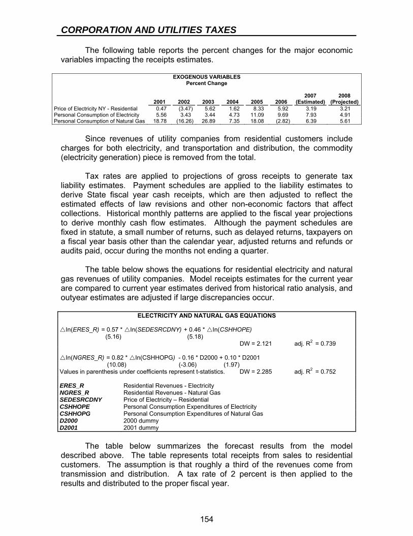
CORPORATION AND UTILITIES TAXES
154
The following table reports the percent changes for the major economic variables impacting the receipts estimates.
EXOGENOUS VARIABLES Percent Change
2007 2008 2001 2002 2003 2004 2005 2006 (Estimated) (Projected)Price of Electricity NY - Residential 0.47 (3.47) 5.62 1.62 8.33 5.92 3.19 3.21 Personal Consumption of Electricity 5.56 3.43 3.44 4.73 11.09 9.69 7.93 4.91 Personal Consumption of Natural Gas 18.78 (16.26) 26.89 7.35 18.08 (2.82) 6.39 5.61
Since revenues of utility companies from residential customers include charges for both electricity, and transportation and distribution, the commodity (electricity generation) piece is removed from the total. Tax rates are applied to projections of gross receipts to generate tax liability estimates. Payment schedules are applied to the liability estimates to derive State fiscal year cash receipts, which are then adjusted to reflect the estimated effects of law revisions and other non-economic factors that affect collections. Historical monthly patterns are applied to the fiscal year projections to derive monthly cash flow estimates. Although the payment schedules are fixed in statute, a small number of returns, such as delayed returns, taxpayers on a fiscal year basis other than the calendar year, adjusted returns and refunds or audits paid, occur during the months not ending a quarter. The table below shows the equations for residential electricity and natural gas revenues of utility companies. Model receipts estimates for the current year are compared to current year estimates derived from historical ratio analysis, and outyear estimates are adjusted if large discrepancies occur.
ELECTRICITY AND NATURAL GAS EQUATIONS
In(ERES_R) = 0.57 * In(SEDESRCDNY) + 0.46 * In(CSHHOPE) (5.16) (5.18) DW = 2.121 adj. R2 = 0.739
In(NGRES_R) = 0.82 * In(CSHHOPG) - 0.16 * D2000 + 0.10 * D2001 (10.08) (-3.06) (1.97) Values in parenthesis under coefficients represent t-statistics. DW = 2.285 adj. R2 = 0.752 ERES_R Residential Revenues - Electricity NGRES_R Residential Revenues - Natural Gas SEDESRCDNY Price of Electricity – Residential CSHHOPE Personal Consumption Expenditures of Electricity CSHHOPG Personal Consumption Expenditures of Natural Gas D2000 2000 dummy D2001 2001 dummy The table below summarizes the forecast results from the model described above. The table represents total receipts from sales to residential customers. The assumption is that roughly a third of the revenues come from transmission and distribution. A tax rate of 2 percent is then applied to the results and distributed to the proper fiscal year.
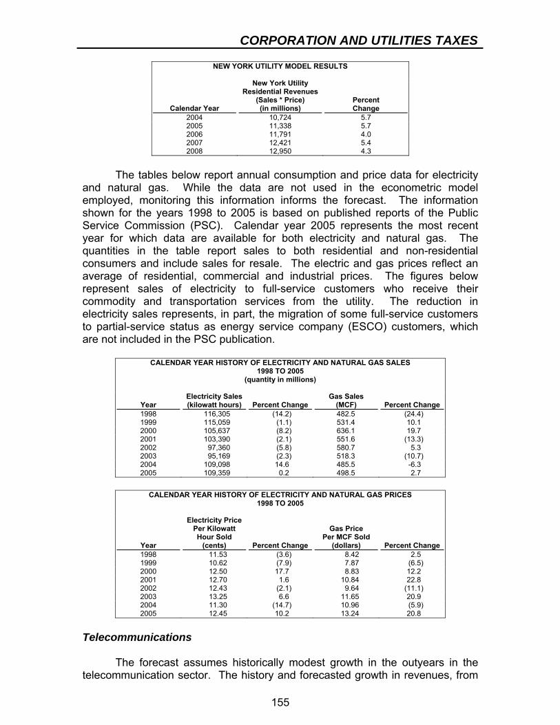
CORPORATION AND UTILITIES TAXES
155
NEW YORK UTILITY MODEL RESULTS
Calendar Year
New York Utility Residential Revenues
(Sales * Price) (in millions)
Percent Change
2004 10,724 5.7 2005 11,338 5.7 2006 11,791 4.0 2007 12,421 5.4 2008 12,950 4.3
The tables below report annual consumption and price data for electricity and natural gas. While the data are not used in the econometric model employed, monitoring this information informs the forecast. The information shown for the years 1998 to 2005 is based on published reports of the Public Service Commission (PSC). Calendar year 2005 represents the most recent year for which data are available for both electricity and natural gas. The quantities in the table report sales to both residential and non-residential consumers and include sales for resale. The electric and gas prices reflect an average of residential, commercial and industrial prices. The figures below represent sales of electricity to full-service customers who receive their commodity and transportation services from the utility. The reduction in electricity sales represents, in part, the migration of some full-service customers to partial-service status as energy service company (ESCO) customers, which are not included in the PSC publication.
CALENDAR YEAR HISTORY OF ELECTRICITY AND NATURAL GAS SALES 1998 TO 2005
(quantity in millions)
Year
Electricity Sales (kilowatt hours)
Percent Change
Gas Sales (MCF)
Percent Change
1998 116,305 (14.2) 482.5 (24.4) 1999 115,059 (1.1) 531.4 10.1 2000 105,637 (8.2) 636.1 19.7 2001 103,390 (2.1) 551.6 (13.3) 2002 97,360 (5.8) 580.7 5.3 2003 95,169 (2.3) 518.3 (10.7) 2004 109,098 14.6 485.5 -6.3 2005 109,359 0.2 498.5 2.7
CALENDAR YEAR HISTORY OF ELECTRICITY AND NATURAL GAS PRICES
1998 TO 2005
Year
Electricity Price Per Kilowatt Hour Sold
(cents)
Percent Change
Gas Price
Per MCF Sold (dollars)
Percent Change 1998 11.53 (3.6) 8.42 2.5 1999 10.62 (7.9) 7.87 (6.5) 2000 12.50 17.7 8.83 12.2 2001 12.70 1.6 10.84 22.8 2002 12.43 (2.1) 9.64 (11.1) 2003 13.25 6.6 11.65 20.9 2004 11.30 (14.7) 10.96 (5.9) 2005 12.45 10.2 13.24 20.8
Telecommunications The forecast assumes historically modest growth in the outyears in the telecommunication sector. The history and forecasted growth in revenues, from
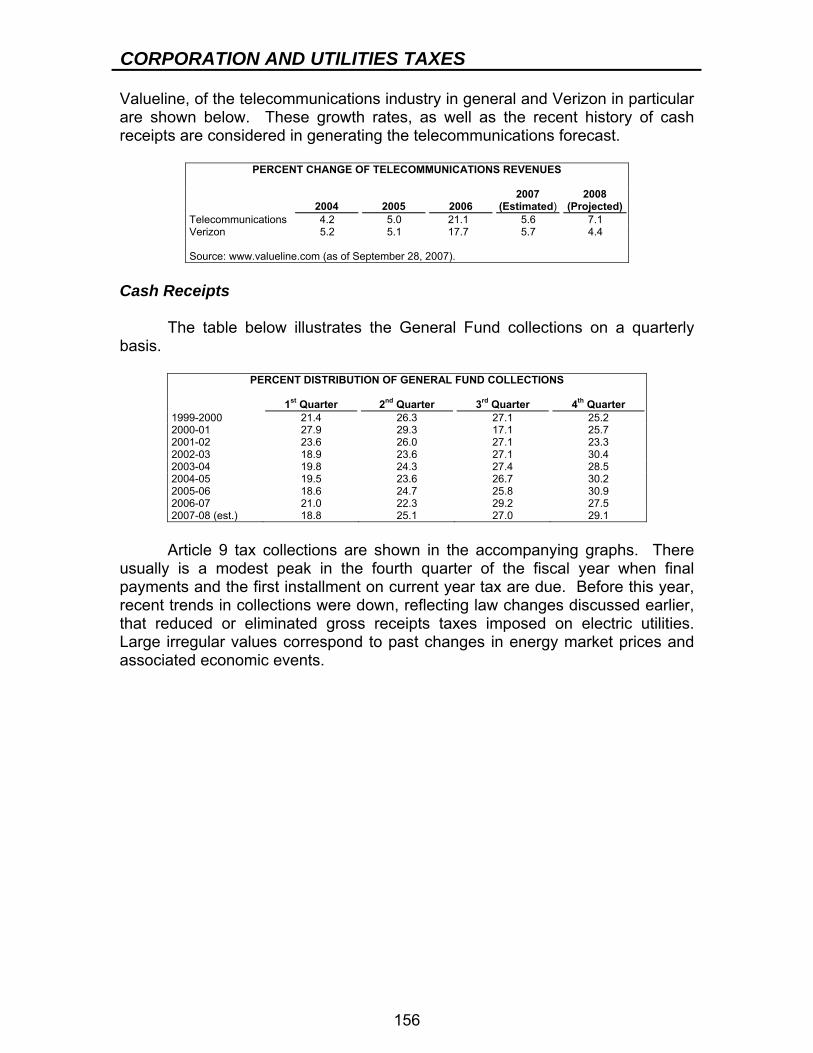
CORPORATION AND UTILITIES TAXES
156
Valueline, of the telecommunications industry in general and Verizon in particular are shown below. These growth rates, as well as the recent history of cash receipts are considered in generating the telecommunications forecast.
PERCENT CHANGE OF TELECOMMUNICATIONS REVENUES
2007 2008 2004 2005 2006 (Estimated) (Projected) Telecommunications 4.2 5.0 21.1 5.6 7.1 Verizon 5.2 5.1 17.7 5.7 4.4 Source: www.valueline.com (as of September 28, 2007).
Cash Receipts The table below illustrates the General Fund collections on a quarterly basis.
PERCENT DISTRIBUTION OF GENERAL FUND COLLECTIONS
1st Quarter 2nd Quarter 3rd Quarter 4th Quarter 1999-2000 21.4 26.3 27.1 25.2 2000-01 27.9 29.3 17.1 25.7 2001-02 23.6 26.0 27.1 23.3 2002-03 18.9 23.6 27.1 30.4 2003-04 19.8 24.3 27.4 28.5 2004-05 19.5 23.6 26.7 30.2 2005-06 18.6 24.7 25.8 30.9 2006-07 21.0 22.3 29.2 27.5 2007-08 (est.) 18.8 25.1 27.0 29.1
Article 9 tax collections are shown in the accompanying graphs. There usually is a modest peak in the fourth quarter of the fiscal year when final payments and the first installment on current year tax are due. Before this year, recent trends in collections were down, reflecting law changes discussed earlier, that reduced or eliminated gross receipts taxes imposed on electric utilities. Large irregular values correspond to past changes in energy market prices and associated economic events.
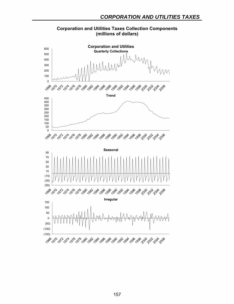
CORPORATION AND UTILITIES TAXES
157
Corporation and Utilities Taxes Collection Components (millions of dollars)
0
100
200
300
400
500
600
1968
1970
1972
1974
1976
1978
1980
1982
1984
1986
1988
1990
1992
1994
1996
1998
2000
2002
2004
2006
Corporation and UtilitiesQuarterly Collections
050
100150200250300350400450
1968
1970
1972
1974
1976
1978
1980
1982
1984
1986
1988
1990
1992
1994
1996
1998
2000
2002
2004
2006
Trend
(50)(30)(10)1030507090
1968
1970
1972
1974
1976
1978
1980
1982
1984
1986
1988
1990
1992
1994
1996
1998
2000
2002
2004
2006
Seasonal
(150)
(100)
(50)
0
50
100
150
1968
1970
1972
1974
1976
1978
1980
1982
1984
1986
1988
1990
1992
1994
1996
1998
2000
2002
2004
2006
Irregular

CORPORATION AND UTILITIES TAXES
158
Risks to the Forecast The corporate and utilities forecasts involve managing uncertainties as follows:
● examining economic factors such as energy prices, changes in supply and demand, business market conditions, changes in technology, and general inflation; and
● analyzing statutory, regulatory and administrative changes, including Federal tax law changes, that affect tax rates and bases.
159
INSURANCE TAXES BACKGROUND Tax Base and Rate The Tax Law imposes a franchise tax on insurance companies and premiums tax on independently procured insurance. The Insurance Law also imposes retaliatory taxes and other premiums taxes on certain insurance brokers. As discussed in more detail below, legislation enacted in 2003 and effective for tax years beginning January 1, 2003 changed the structure of the insurance tax. Life Insurers For life insurers, the tax structure includes two components. The first component is an income-based tax computed on the highest of four bases, plus a tax on subsidiary capital. The second component is a tax based on gross direct premiums, less return premiums thereon, written on risks located or resident in New York. Minimum and maximum limitations are applied to total tax liability before credits. The minimum limitation is 1.5 percent of premiums and the maximum limitation is 2 percent of premiums. The income component is imposed on one of several measures of an insurance corporation’s economic activity within the State. Most taxpayers pay under the entire net income (ENI) base. For taxable years starting on and after January 1, 2007, the tax rate on ENI equals 7.1 percent. Taxpayers allocate receipts according to the ratio of New York premiums and payroll to total premiums and payroll nationwide. The following chart depicts the structure of the insurance tax imposed on life insurers.
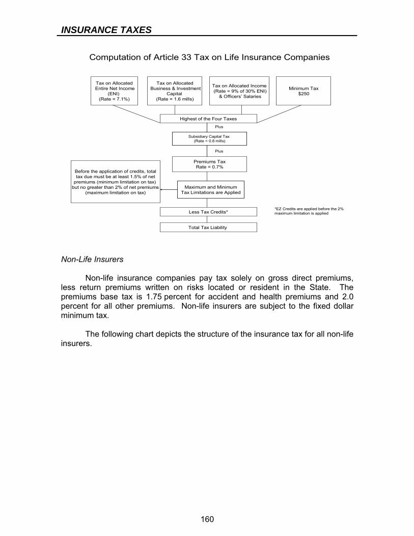
INSURANCE TAXES
160
Computation of Article 33 Tax on Life Insurance Companies
Tax on AllocatedEntire Net Income
(ENI) (Rate = 7.1%)
Tax on AllocatedBusiness & Investment
Capital (Rate = 1.6 mills)
Tax on Allocated Income(Rate = 9% of 30% ENI)
& Officers’ Salaries
Minimum Tax$250
Highest of the Four Taxes
Premiums TaxRate = 0.7%
Plus
Less Tax Credits*
Total Tax Liability
Subsidiary Capital Tax (Rate = 0.8 mills)
Plus
Maximum and MinimumTax Limitations are Applied
*EZ Credits are applied before the 2% maximum limitation is applied
Before the application of credits, totaltax due must be at least 1.5% of net
premiums (minimum limitation on tax) but no greater than 2% of net premiums
(maximum limitation on tax)
Non-Life Insurers Non-life insurance companies pay tax solely on gross direct premiums, less return premiums written on risks located or resident in the State. The premiums base tax is 1.75 percent for accident and health premiums and 2.0 percent for all other premiums. Non-life insurers are subject to the fixed dollar minimum tax. The following chart depicts the structure of the insurance tax for all non-life insurers.
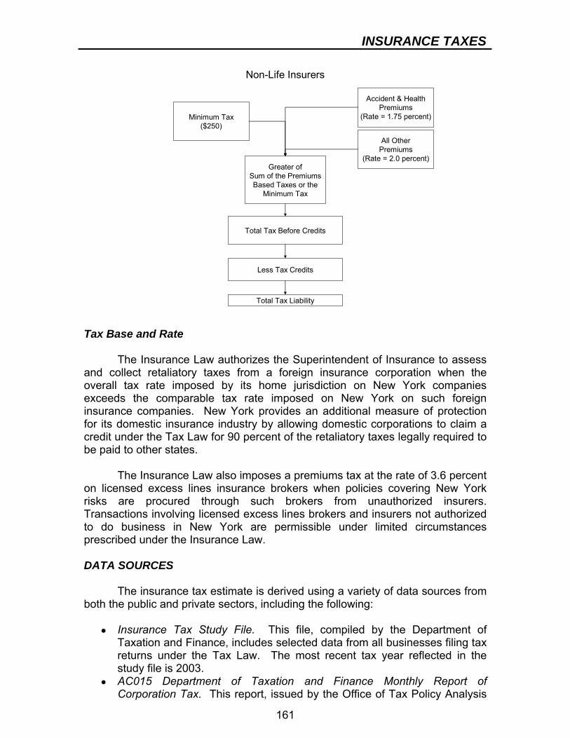
INSURANCE TAXES
161
Accident & HealthPremiums
(Rate = 1.75 percent)
Greater ofSum of the PremiumsBased Taxes or the
Minimum Tax
Total Tax Before Credits
Less Tax Credits
Total Tax Liability
Non-Life Insurers
Minimum Tax($250)
All OtherPremiums
(Rate = 2.0 percent)
Tax Base and Rate The Insurance Law authorizes the Superintendent of Insurance to assess and collect retaliatory taxes from a foreign insurance corporation when the overall tax rate imposed by its home jurisdiction on New York companies exceeds the comparable tax rate imposed on New York on such foreign insurance companies. New York provides an additional measure of protection for its domestic insurance industry by allowing domestic corporations to claim a credit under the Tax Law for 90 percent of the retaliatory taxes legally required to be paid to other states. The Insurance Law also imposes a premiums tax at the rate of 3.6 percent on licensed excess lines insurance brokers when policies covering New York risks are procured through such brokers from unauthorized insurers. Transactions involving licensed excess lines brokers and insurers not authorized to do business in New York are permissible under limited circumstances prescribed under the Insurance Law. DATA SOURCES The insurance tax estimate is derived using a variety of data sources from both the public and private sectors, including the following:
● Insurance Tax Study File. This file, compiled by the Department of Taxation and Finance, includes selected data from all businesses filing tax returns under the Tax Law. The most recent tax year reflected in the study file is 2003.
● AC015 Department of Taxation and Finance Monthly Report of Corporation Tax. This report, issued by the Office of Tax Policy Analysis
INSURANCE TAXES
162
(OTPA) at the New York State Department of Taxation and Finance, provides reconciled monthly collections of insurance tax receipts by filing periods.
● New York State Corporate Tax Statistical Report. This report is published by the Department of Taxation and Finance’s OTPA. It provides a detailed summary of insurance tax data. The most recent report is for tax year 2003.
● Value Line Investment Survey. Insurance Industry. ● Securities and Exchange Commission (SEC) Website. This web site is
monitored for relevant quarterly (10-Q) and annual (10-K) financial reports. ● New York State Insurance Department. Detail on lines of property and
casualty insurance and data from premiums taxes and retaliatory taxes imposed under the Insurance Law.
● Other Publications. Wall Street Journal, New York Times, Business Week, Barron's, A.M. Best Review, and Crain’s.
STATUTORY CHANGES Effective in tax years beginning January 1, 2003, legislation changed the tax imposed on non-life insurance companies from a franchise tax based on income to a franchise tax based solely on gross direct premiums less return premiums. Accident and health premiums are subject to a tax rate of 1.75 percent, and all other non-life premiums are subject to a tax rate of 2 percent. Non-life insurance companies are subject to a minimum tax of $250. The structure of the franchise tax on income imposed on life insurance companies was not changed; however, a minimum tax of no less than 1.5 percent of premiums (computed prior to the application of tax credits) was imposed. Effective in tax years beginning January 1, 2007, the rate imposed on the ENI base for life insurers was changed from 7.5 percent to 7.1 percent. For a detailed list of significant statutory changes made to the insurance tax, please see the 2007-08 New York State Executive Budget - Economic and Revenue Outlook. FORECAST METHODOLOGY The estimates for the current year and the outyears are based on a blend of historical collection patterns, simple trending techniques, estimates of underlying company liability, econometric models for key components of the base sensitive to economic or consumption changes, and statutory changes or other occurrences that may impact collections. Insurance premiums are divided into three broad categories: property and casualty, life and health, and accident and health, sold by non-life insurance companies. Net income is aggregated over life insurance companies and modeled separately. The insurance tax model currently uses four equations to estimate liability for life insurance, accident and health, ENI, and property and casualty, as are discussed later in a table.
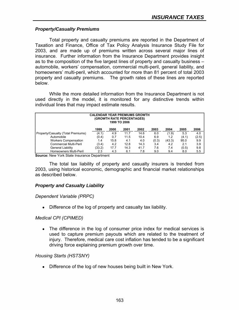
INSURANCE TAXES
163
Property/Casualty Premiums Total property and casualty premiums are reported in the Department of Taxation and Finance, Office of Tax Policy Analysis Insurance Study File for 2003, and are made up of premiums written across several major lines of insurance. Further information from the Insurance Department provides insight as to the composition of the five largest lines of property and casualty business – automobile, workers’ compensation, commercial multi-peril, general liability, and homeowners’ multi-peril, which accounted for more than 81 percent of total 2003 property and casualty premiums. The growth rates of these lines are reported below. While the more detailed information from the Insurance Department is not used directly in the model, it is monitored for any distinctive trends within individual lines that may impact estimate results.
CALENDAR YEAR PREMIUMS GROWTH (GROWTH RATE PERCENTAGES)
1999 TO 2006
1999 2000 2001 2002 2003 2004 2005 2006 Property/Casualty (Total Premiums) (4.1) 4.9 11.7 14.6 6.0 (1.9) 5.3 4.0 Automobile (0.4) 0.7 11.5 10.4 6.9 1.2 (4.1) (2.5) Workers Compensation 1.4 15.8 4.1 4.0 (0.3) (43.3) 95.0 9.9 Commercial Multi-Peril (3.4) 4.2 12.8 14.3 3.4 4.2 2.1 3.9 General Liability (33.2) 17.7 14.3 41.7 7.6 7.4 (0.5) 9.8 Homeowners Multi-Peril 2.3 4.3 6.1 7.8 9.0 9.4 8.0 5.5
Source: New York State Insurance Department The total tax liability of property and casualty insurers is trended from 2003, using historical economic, demographic and financial market relationships as described below. Property and Casualty Liability Dependent Variable (PRPC)
● Difference of the log of property and casualty tax liability. Medical CPI (CPIMED)
● The difference in the log of consumer price index for medical services is used to capture premium payouts which are related to the treatment of injury. Therefore, medical care cost inflation has tended to be a significant driving force explaining premium growth over time.
Housing Starts (HSTSNY)
● Difference of the log of new houses being built in New York.
INSURANCE TAXES
164
Dummy Variable 2001 and 2002 (D0102)
● The model also includes a dummy variable for 2001 and 2002 to account for significant changes due to September 11, 2001. The dummy has a value of one for 2001 and 2002 when premiums grew extraordinarily in order to recover cost increases, and zero otherwise.
Dummy Variable for 1988 (D88)
● Used to capture extraordinary fluctuations in the data series. Life Insurance Liability Dependent Variable (PRLH)
● Difference in the log of life insurance liability. Medical CPI (CPIMED)
● This variable is used to capture increases in healthcare costs. Tax Rate (THL)
● The tax difference in the tax rate for life/health is included to capture responses in premiums to tax law changes.
Residential Population Ages 0 to 24 (NR024NY)
● First difference in the log of resident population ages 0 to 24. This variable is included to reflect the fact that people tend to get accident/health insurance when they have children.
Dummy Variable 1998 (D98)
● The dummy has a value of one if 1998, or 0 otherwise, to account for large fluctuations in premiums during that year.
Dummy Variable 2001(D01)
● The model also includes a dummy variable for 2001 to account for significant changes due to the events of September 11, 2001.
Accident/Health Liability Dependent Variable (PRAH)
● Difference in the log of accident/health liability.
INSURANCE TAXES
165
Housing Starts in New York (HSTSNY)
● First difference in the log of housing starts in New York. As home ownership increases, it is assumed that accident/health insurance coverage will increase as well. A three-year lag of this variable is also included, suggesting a three-year lag in coverage for a considerable share of new homeowners.
Medical CPI - 1992 (TrendCPI)
● Rate of inflation of medical costs, indexed to 1992. Dummy Variable 1991 and 1992 (D91_92)
● The dummy has a value of one if 1991, negative one if 1992, or 0 otherwise.
Liability From Entire Net Income Base Dependent Variable (TXENI)
● First difference in the tax collected on entire net income. Starting with the 2003 tax year, only life insurers calculate the entire net income base in arriving at their tax liability. Model results are scrutinized for this large change in the tax base, and future changes to the estimation methodology may be necessary as a result.
10-Year Treasury Bond Rate (TRATE10)
● The first difference in the ten-year Treasury note rate. Dummy Variable 2001 and 2002 (D01_02)
● The dummy has a value of one if 2001, negative one if 2002, or 0 otherwise.
To further refine the net income estimate, an analysis of industry trends with particular attention to industry leaders is used. Several publications, including Value Line and Best’s, provide estimates of the future earnings of the industry as a whole and industry leaders with a large New York presence.
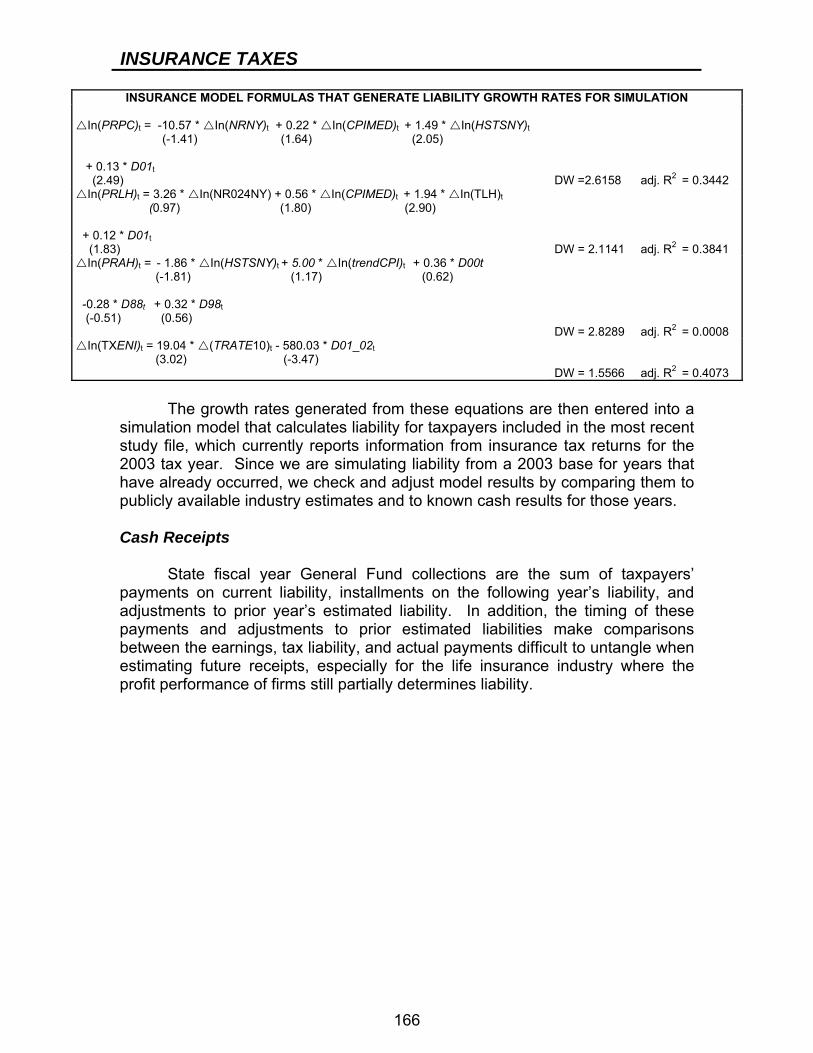
INSURANCE TAXES
166
INSURANCE MODEL FORMULAS THAT GENERATE LIABILITY GROWTH RATES FOR SIMULATION
In(PRPC)t = -10.57 * In(NRNY)t + 0.22 * In(CPIMED)t + 1.49 * In(HSTSNY)t (-1.41) (1.64) (2.05) + 0.13 * D01t (2.49) DW =2.6158 adj. R2 = 0.3442
In(PRLH)t = 3.26 * In(NR024NY) + 0.56 * In(CPIMED)t + 1.94 * In(TLH)t (0.97) (1.80) (2.90) + 0.12 * D01t (1.83) DW = 2.1141 adj. R2 = 0.3841
In(PRAH)t = - 1.86 * In(HSTSNY)t + 5.00 * In(trendCPI)t + 0.36 * D00t (-1.81) (1.17) (0.62) -0.28 * D88t + 0.32 * D98t (-0.51) (0.56) DW = 2.8289 adj. R2 = 0.0008
In(TXENI)t = 19.04 * (TRATE10)t - 580.03 * D01_02t (3.02) (-3.47) DW = 1.5566 adj. R2 = 0.4073
The growth rates generated from these equations are then entered into a simulation model that calculates liability for taxpayers included in the most recent study file, which currently reports information from insurance tax returns for the 2003 tax year. Since we are simulating liability from a 2003 base for years that have already occurred, we check and adjust model results by comparing them to publicly available industry estimates and to known cash results for those years. Cash Receipts State fiscal year General Fund collections are the sum of taxpayers’ payments on current liability, installments on the following year’s liability, and adjustments to prior year’s estimated liability. In addition, the timing of these payments and adjustments to prior estimated liabilities make comparisons between the earnings, tax liability, and actual payments difficult to untangle when estimating future receipts, especially for the life insurance industry where the profit performance of firms still partially determines liability.
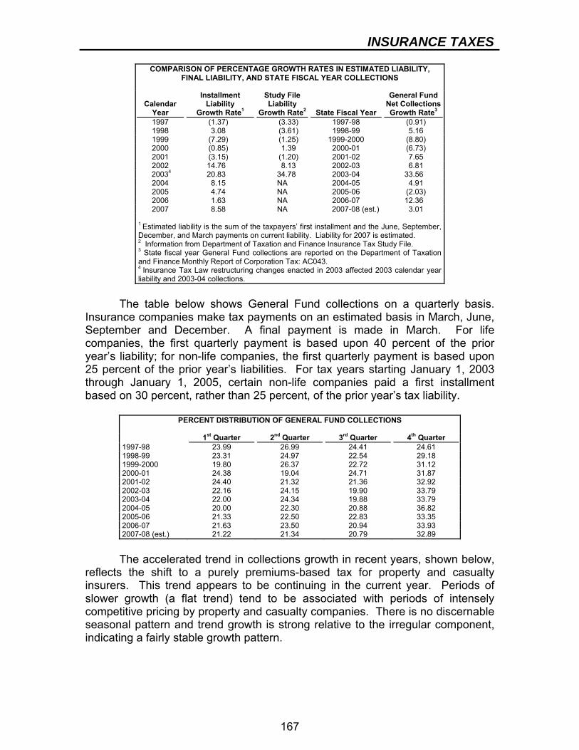
INSURANCE TAXES
167
COMPARISON OF PERCENTAGE GROWTH RATES IN ESTIMATED LIABILITY, FINAL LIABILITY, AND STATE FISCAL YEAR COLLECTIONS
Calendar Year
Installment Liability
Growth Rate1
Study File Liability
Growth Rate2
State Fiscal Year
General Fund Net Collections Growth Rate3
1997 (1.37) (3.33) 1997-98 (0.91) 1998 3.08 (3.61) 1998-99 5.16 1999 (7.29) (1.25) 1999-2000 (8.80) 2000 (0.85) 1.39 2000-01 (6.73) 2001 (3.15) (1.20) 2001-02 7.65 2002 14.76 8.13 2002-03 6.81
20034 20.83 34.78 2003-04 33.56 2004 8.15 NA 2004-05 4.91 2005 4.74 NA 2005-06 (2.03) 2006 1.63 NA 2006-07 12.36 2007 8.58 NA 2007-08 (est.) 3.01
1 Estimated liability is the sum of the taxpayers’ first installment and the June, September, December, and March payments on current liability. Liability for 2007 is estimated. 2 Information from Department of Taxation and Finance Insurance Tax Study File. 3 State fiscal year General Fund collections are reported on the Department of Taxation and Finance Monthly Report of Corporation Tax: AC043. 4 Insurance Tax Law restructuring changes enacted in 2003 affected 2003 calendar year liability and 2003-04 collections.
The table below shows General Fund collections on a quarterly basis. Insurance companies make tax payments on an estimated basis in March, June, September and December. A final payment is made in March. For life companies, the first quarterly payment is based upon 40 percent of the prior year’s liability; for non-life companies, the first quarterly payment is based upon 25 percent of the prior year’s liabilities. For tax years starting January 1, 2003 through January 1, 2005, certain non-life companies paid a first installment based on 30 percent, rather than 25 percent, of the prior year’s tax liability.
PERCENT DISTRIBUTION OF GENERAL FUND COLLECTIONS
1st Quarter 2nd Quarter 3rd Quarter 4th Quarter 1997-98 23.99 26.99 24.41 24.61 1998-99 23.31 24.97 22.54 29.18 1999-2000 19.80 26.37 22.72 31.12 2000-01 24.38 19.04 24.71 31.87 2001-02 24.40 21.32 21.36 32.92 2002-03 22.16 24.15 19.90 33.79 2003-04 22.00 24.34 19.88 33.79 2004-05 20.00 22.30 20.88 36.82 2005-06 21.33 22.50 22.83 33.35 2006-07 21.63 23.50 20.94 33.93 2007-08 (est.) 21.22 21.34 20.79 32.89
The accelerated trend in collections growth in recent years, shown below, reflects the shift to a purely premiums-based tax for property and casualty insurers. This trend appears to be continuing in the current year. Periods of slower growth (a flat trend) tend to be associated with periods of intensely competitive pricing by property and casualty companies. There is no discernable seasonal pattern and trend growth is strong relative to the irregular component, indicating a fairly stable growth pattern.
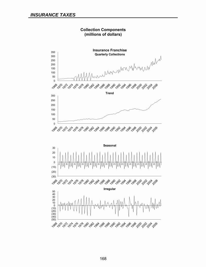
INSURANCE TAXES
168
Collection Components
(millions of dollars)
050
100150200250300350
1968
1970
1972
1974
1976
1978
1980
1982
1984
1986
1988
1990
1992
1994
1996
1998
2000
2002
2004
2006
Insurance FranchiseQuarterly Collections
0
50
100
150
200
250
300
1968
1970
1972
1974
1976
1978
1980
1982
1984
1986
1988
1990
1992
1994
1996
1998
2000
2002
2004
2006
Trend
(30)
(20)
(10)
0
10
20
30
1968
1970
1972
1974
1976
1978
1980
1982
1984
1986
1988
1990
1992
1994
1996
1998
2000
2002
2004
2006
Seasonal
(50)(40)(30)(20)(10)
01020304050
1968
1970
1972
1974
1976
1978
1980
1982
1984
1986
1988
1990
1992
1994
1996
1998
2000
2002
2004
2006
Irregular

INSURANCE TAXES
169
Risks to the Forecast The insurance forecast involves managing uncertainty about turning points in the premiums cycle, and therefore premiums growth, caused by:
● the underwriting discipline and performance of industry members; ● changes in surplus and reserves resulting from investment portfolio and
annuity sales and results; ● changes in the demographic and competitive environment, including
regulatory changes; and ● unexpected weather-related or other catastrophes.
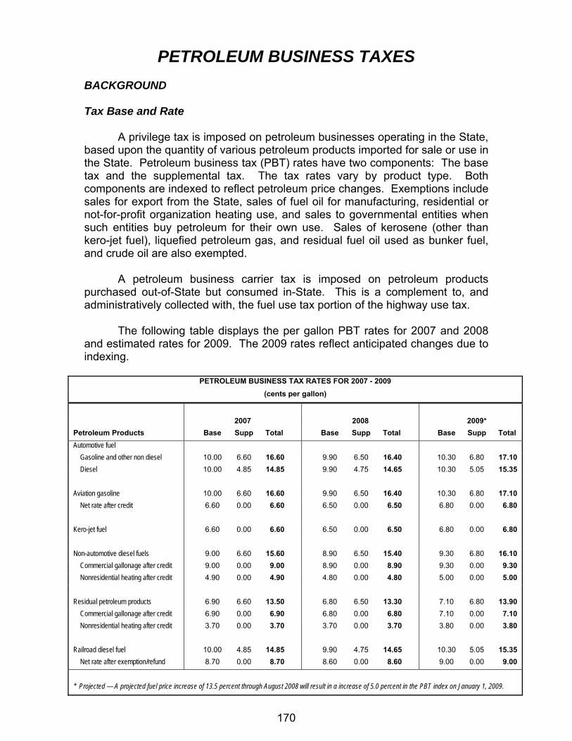
170
PETROLEUM BUSINESS TAXES BACKGROUND Tax Base and Rate A privilege tax is imposed on petroleum businesses operating in the State, based upon the quantity of various petroleum products imported for sale or use in the State. Petroleum business tax (PBT) rates have two components: The base tax and the supplemental tax. The tax rates vary by product type. Both components are indexed to reflect petroleum price changes. Exemptions include sales for export from the State, sales of fuel oil for manufacturing, residential or not-for-profit organization heating use, and sales to governmental entities when such entities buy petroleum for their own use. Sales of kerosene (other than kero-jet fuel), liquefied petroleum gas, and residual fuel oil used as bunker fuel, and crude oil are also exempted. A petroleum business carrier tax is imposed on petroleum products purchased out-of-State but consumed in-State. This is a complement to, and administratively collected with, the fuel use tax portion of the highway use tax. The following table displays the per gallon PBT rates for 2007 and 2008 and estimated rates for 2009. The 2009 rates reflect anticipated changes due to indexing.
PETROLEUM BUSINESS TAX RATES FOR 2007 - 2009 (cents per gallon)
2007 2008 2009* Petroleum Products Base Supp Total Base Supp Total Base Supp Total Automotive fuel Gasoline and other non diesel 10.00 6.60 16.60 9.90 6.50 16.40 10.30 6.80 17.10 Diesel 10.00 4.85 14.85 9.90 4.75 14.65 10.30 5.05 15.35 Aviation gasoline 10.00 6.60 16.60 9.90 6.50 16.40 10.30 6.80 17.10 Net rate after credit 6.60 0.00 6.60 6.50 0.00 6.50 6.80 0.00 6.80 Kero-jet fuel 6.60 0.00 6.60 6.50 0.00 6.50 6.80 0.00 6.80 Non-automotive diesel fuels 9.00 6.60 15.60 8.90 6.50 15.40 9.30 6.80 16.10 Commercial gallonage after credit 9.00 0.00 9.00 8.90 0.00 8.90 9.30 0.00 9.30 Nonresidential heating after credit 4.90 0.00 4.90 4.80 0.00 4.80 5.00 0.00 5.00 Residual petroleum products 6.90 6.60 13.50 6.80 6.50 13.30 7.10 6.80 13.90 Commercial gallonage after credit 6.90 0.00 6.90 6.80 0.00 6.80 7.10 0.00 7.10 Nonresidential heating after credit 3.70 0.00 3.70 3.70 0.00 3.70 3.80 0.00 3.80 Railroad diesel fuel 10.00 4.85 14.85 9.90 4.75 14.65 10.30 5.05 15.35 Net rate after exemption/refund 8.70 0.00 8.70 8.60 0.00 8.60 9.00 0.00 9.00 * Projected — A projected fuel price increase of 13.5 percent through August 2008 will result in a increase of 5.0 percent in the PBT index on January 1, 2009.
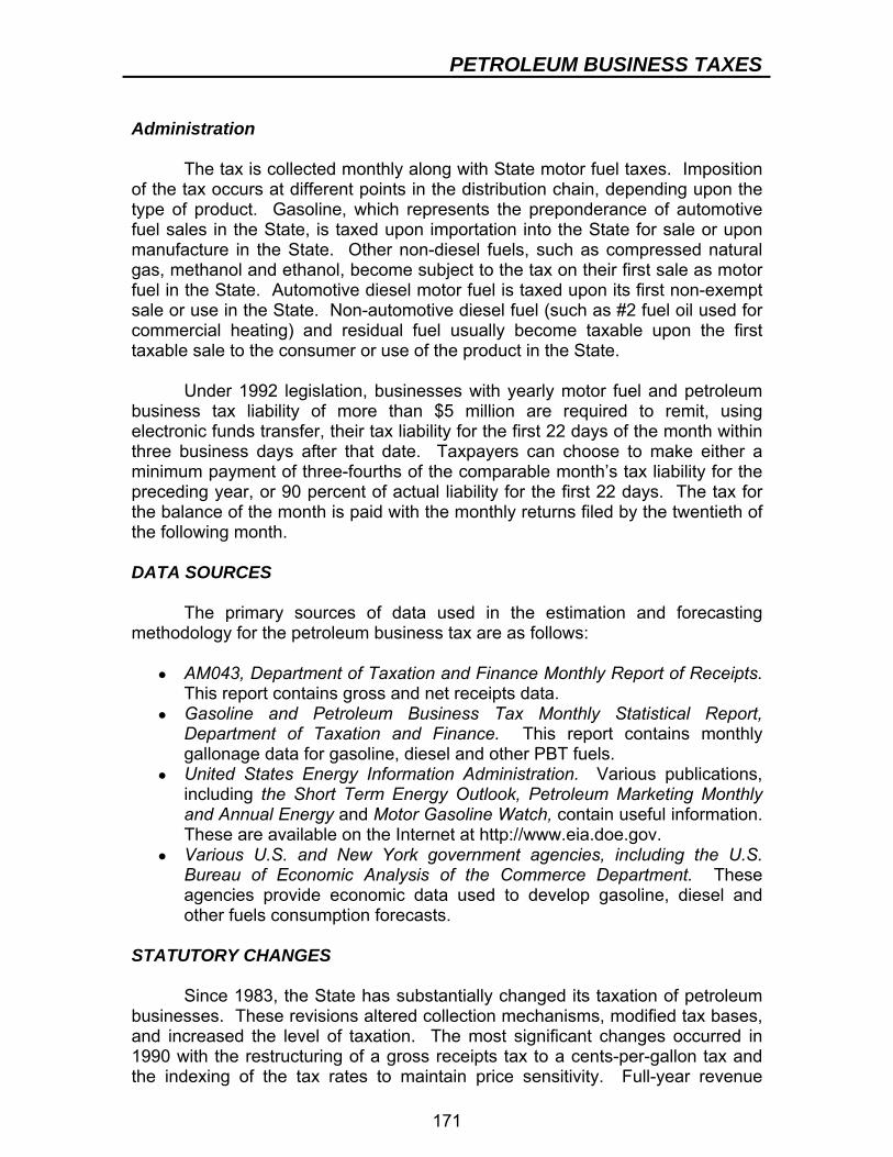
PETROLEUM BUSINESS TAXES
171
Administration The tax is collected monthly along with State motor fuel taxes. Imposition of the tax occurs at different points in the distribution chain, depending upon the type of product. Gasoline, which represents the preponderance of automotive fuel sales in the State, is taxed upon importation into the State for sale or upon manufacture in the State. Other non-diesel fuels, such as compressed natural gas, methanol and ethanol, become subject to the tax on their first sale as motor fuel in the State. Automotive diesel motor fuel is taxed upon its first non-exempt sale or use in the State. Non-automotive diesel fuel (such as #2 fuel oil used for commercial heating) and residual fuel usually become taxable upon the first taxable sale to the consumer or use of the product in the State. Under 1992 legislation, businesses with yearly motor fuel and petroleum business tax liability of more than $5 million are required to remit, using electronic funds transfer, their tax liability for the first 22 days of the month within three business days after that date. Taxpayers can choose to make either a minimum payment of three-fourths of the comparable month’s tax liability for the preceding year, or 90 percent of actual liability for the first 22 days. The tax for the balance of the month is paid with the monthly returns filed by the twentieth of the following month. DATA SOURCES The primary sources of data used in the estimation and forecasting methodology for the petroleum business tax are as follows:
● AM043, Department of Taxation and Finance Monthly Report of Receipts. This report contains gross and net receipts data.
● Gasoline and Petroleum Business Tax Monthly Statistical Report, Department of Taxation and Finance. This report contains monthly gallonage data for gasoline, diesel and other PBT fuels.
● United States Energy Information Administration. Various publications, including the Short Term Energy Outlook, Petroleum Marketing Monthly and Annual Energy and Motor Gasoline Watch, contain useful information. These are available on the Internet at http://www.eia.doe.gov.
● Various U.S. and New York government agencies, including the U.S. Bureau of Economic Analysis of the Commerce Department. These agencies provide economic data used to develop gasoline, diesel and other fuels consumption forecasts.
STATUTORY CHANGES Since 1983, the State has substantially changed its taxation of petroleum businesses. These revisions altered collection mechanisms, modified tax bases, and increased the level of taxation. The most significant changes occurred in 1990 with the restructuring of a gross receipts tax to a cents-per-gallon tax and the indexing of the tax rates to maintain price sensitivity. Full-year revenue
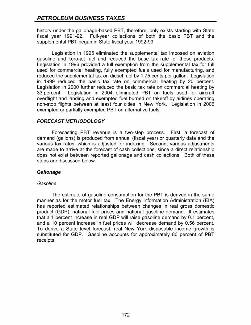
PETROLEUM BUSINESS TAXES
172
history under the gallonage-based PBT, therefore, only exists starting with State fiscal year 1991-92. Full-year collections of both the basic PBT and the supplemental PBT began in State fiscal year 1992-93. Legislation in 1995 eliminated the supplemental tax imposed on aviation gasoline and kero-jet fuel and reduced the base tax rate for those products. Legislation in 1996 provided a full exemption from the supplemental tax for full used for commercial heating, fully exempted fuels used for manufacturing, and reduced the supplemental tax on diesel fuel by 1.75 cents per gallon. Legislation in 1999 reduced the basic tax rate on commercial heating by 20 percent. Legislation in 2000 further reduced the basic tax rate on commercial heating by 33 percent. Legislation in 2004 eliminated PBT on fuels used for aircraft overflight and landing and exempted fuel burned on takeoff by airlines operating non-stop flights between at least four cities in New York. Legislation in 2006 exempted or partially exempted PBT on alternative fuels. FORECAST METHODOLOGY Forecasting PBT revenue is a two-step process. First, a forecast of demand (gallons) is produced from annual (fiscal year) or quarterly data and the various tax rates, which is adjusted for indexing. Second, various adjustments are made to arrive at the forecast of cash collections, since a direct relationship does not exist between reported gallonage and cash collections. Both of these steps are discussed below. Gallonage Gasoline The estimate of gasoline consumption for the PBT is derived in the same manner as for the motor fuel tax. The Energy Information Administration (EIA) has reported estimated relationships between changes in real gross domestic product (GDP), national fuel prices and national gasoline demand. It estimates that a 1 percent increase in real GDP will raise gasoline demand by 0.1 percent, and a 10 percent increase in fuel prices will decrease demand by 0.56 percent. To derive a State level forecast, real New York disposable income growth is substituted for GDP. Gasoline accounts for approximately 80 percent of PBT receipts.
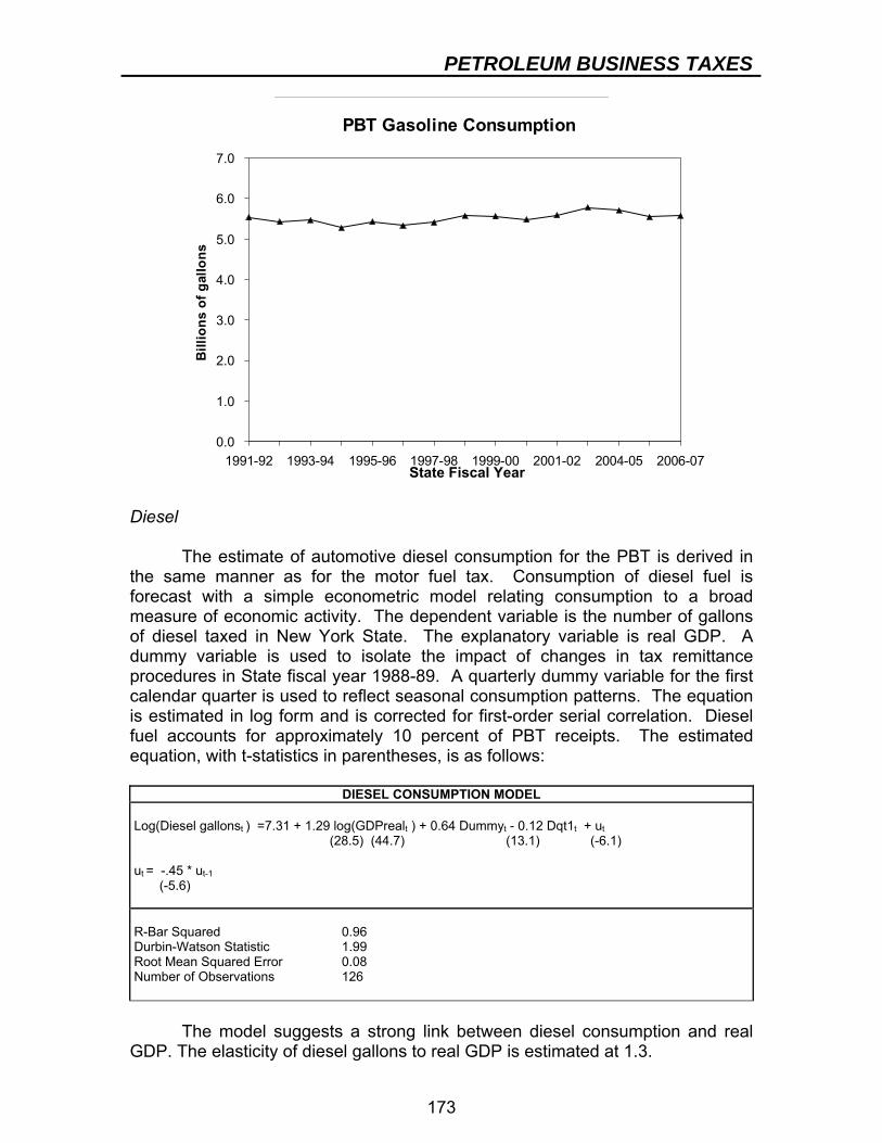
PETROLEUM BUSINESS TAXES
173
PERCENT CHANGE IN EXOGENOUS VARIABLES
Real NY
Disposable IncomeNY
Gasoline Price 1996-97 1.9 7.8 1997-98 2.4 (5.0) 1998-99 4.2 (12.4) 1999-2000 0.9 21.7 2000-01 4.1 18.6 2001-02 (0.1) (9.3) 2002-03 3.0 5.7 2003-04 2.8 8.8 2004-05 2.6 20.0 2005-06 -0.6 23.2 2006-07 1.1 8.8 2007-08 (est.) 2.9 3.2
Diesel The estimate of automotive diesel consumption for the PBT is derived in the same manner as for the motor fuel tax. Consumption of diesel fuel is forecast with a simple econometric model relating consumption to a broad measure of economic activity. The dependent variable is the number of gallons of diesel taxed in New York State. The explanatory variable is real GDP. A dummy variable is used to isolate the impact of changes in tax remittance procedures in State fiscal year 1988-89. A quarterly dummy variable for the first calendar quarter is used to reflect seasonal consumption patterns. The equation is estimated in log form and is corrected for first-order serial correlation. Diesel fuel accounts for approximately 10 percent of PBT receipts. The estimated equation, with t-statistics in parentheses, is as follows:
DIESEL CONSUMPTION MODEL Log(Diesel gallonst ) =7.31 + 1.29 log(GDPrealt ) + 0.64 Dummyt - 0.12 Dqt1t + ut (28.5) (44.7) (13.1) (-6.1) ut = -.45 * ut-1 (-5.6) R-Bar Squared 0.96 Durbin-Watson Statistic 1.99 Root Mean Squared Error 0.08 Number of Observations 126 The model suggests a strong link between diesel consumption and real GDP. The elasticity of diesel gallons to real GDP is estimated at 1.3.
PBT Gasoline Consumption
0.0
1.0
2.0
3.0
4.0
5.0
6.0
7.0
1991-92 1993-94 1995-96 1997-98 1999-00 2001-02 2004-05 2006-07
Bill
ions
of g
allo
ns
State Fiscal Year

PETROLEUM BUSINESS TAXES
174
Utility Residual Fuels Residual fuels are burned by electric utilities to produce electricity. They can switch to natural gas (which is not subject to the PBT) depending upon relative prices and State regulatory policy, which requires utilities to burn residual fuels during times of high residential demand for natural gas. On average, residual fuel accounts for more than 5 percent of PBT receipts. Rates/Indexing Since 1990, basic and supplemental PBT tax rates have been subject to separately computed annual adjustments on January 1 of each year to reflect the change in the Producer Price Index for refined petroleum products (PPI) for the 12 months ending August 31 of the immediately preceding year. The tax rates, therefore, increase as prices rise and decrease as prices fall. The monthly history of the PPI is published by the Bureau of Labor Statistics of the United States Department of Labor. The Division of the Budget forecasts the PPI based on historical data. Beginning January 1, 1996, the PBT rate index has been adjusted annually subject to a maximum change of 5 percent of the current rate in any year. As a result, the PBT rate index decreased by 5 percent on January 1, 2003, and increased by 5 percent on January 1, 2004 through January 1, 2007. The PBT index will decrease by 1.2 percent on January 1, 2008. It should be noted that, in general, the statute also requires the base and the supplemental gasoline rates to be rounded to the nearest tenth of one cent. As a result, the actual increases or decreases in the tax rates from indexing are usually slightly different than the full percentage change dictated by the tax rate index. Rates are also affected by statutory changes that may complement or offset the changes due to indexing. Adjustments After generating a demand forecast and applying the appropriate tax rates, adjustments are made for refunds, credits, pay schedule lags, accounting delays, historical and year-to-date collection patterns and tax law and administrative changes. Cash Receipts See Motor Fuel section for component graphs for gasoline and diesel taxes.
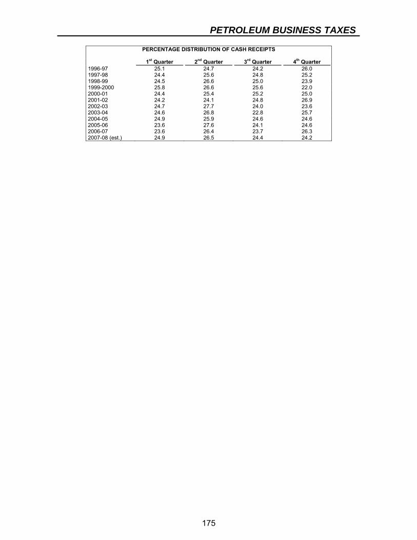
PETROLEUM BUSINESS TAXES
175
PERCENTAGE DISTRIBUTION OF CASH RECEIPTS
1st Quarter 2nd Quarter 3rd Quarter 4th Quarter 1996-97 25.1 24.7 24.2 26.0 1997-98 24.4 25.6 24.8 25.2 1998-99 24.5 26.6 25.0 23.9 1999-2000 25.8 26.6 25.6 22.0 2000-01 24.4 25.4 25.2 25.0 2001-02 24.2 24.1 24.8 26.9 2002-03 24.7 27.7 24.0 23.6 2003-04 24.6 26.8 22.8 25.7 2004-05 24.9 25.9 24.6 24.6 2005-06 23.6 27.6 24.1 24.6 2006-07 23.6 26.4 23.7 26.3 2007-08 (est.) 24.9 26.5 24.4 24.2
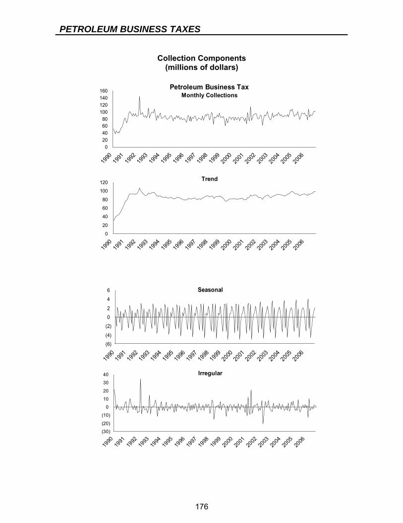
PETROLEUM BUSINESS TAXES
176
Collection Components
(millions of dollars)
020406080
100120140160
1990
1991
1992
1993
1994
1995
1996
1997
1998
1999
2000
2001
2002
2003
2004
2005
2006
Petroleum Business TaxMonthly Collections
0
20
40
60
80
100
120
1990
1991
1992
1993
1994
1995
1996
1997
1998
1999
2000
2001
2002
2003
2004
2005
2006
Trend
(6)
(4)
(2)
0
2
4
6
1990
1991
1992
1993
1994
1995
1996
1997
1998
1999
2000
2001
2002
2003
2004
2005
2006
Seasonal
(30)
(20)
(10)
0
10
20
30
40
1990
1991
1992
1993
1994
1995
1996
1997
1998
1999
2000
2001
2002
2003
2004
2005
2006
Irregular
PETROLEUM BUSINESS TAXES
177
Risks to the Forecast Historically, PBT receipts have remained relatively stable under a wide variety of political and economic conditions. However, due to the difficulty in predicting fuel prices, inventories, and weather conditions, the current PBT revenue estimate has some inherent risks. Among these risks, the variation of fuel prices is the most noteworthy. Global economic and political conditions, as well as market forces, can affect fuel prices. For example, between January 1999 and October 1999, the world crude oil price increased by 116 percent. More recently, gasoline and diesel fuel prices have fluctuated by more than sixty cents in 2006. Changes in fuel prices may change fuel consumption, especially residual fuel consumption. The growth rate of utility residual fuel consumption exhibited volatility during the last five years, ranging from a negative 56 percent to a positive 147 percent. Fuel price changes may also change fuel inventories, the PBT index, and tax rates.
178
ESTATE TAX TAX BASE AND RATE New York imposes a tax on the estates of deceased State residents and on that part of a nonresident’s estate made up of real and tangible personal property located within New York State. The New York estate tax is based on the estate tax provisions of the Federal Internal Revenue Code as amended through July 22, 1998, with New York modifications. The tax base is calculated by first determining the value of the gross estate using Federal estate tax provisions. The Federal gross estate comprises the total amount of real estate, stocks and bonds, mortgages, notes, cash, insurance on decedent's life, jointly owned property, other miscellaneous property, transfers during decedent's life, powers of appointment, and annuities that the decedent owned. The Federal gross estate is reduced by the Qualified Conservation Easement Exclusion and the following deductions: funeral expenses and expenses incurred in administering property subject to claims; debts of the decedent; mortgages and liens; net losses during administration; expenses incurred in administration of the property not subject to claims; bequests to a surviving spouse (marriage deduction); charitable, public, and similar gifts; and a qualified family-owned business interest deduction. This yields the taxable estate for New York and becomes the basis for calculating New York’s estate tax. The total value of all items of real and tangible personal property of the taxpayer located outside of New York State is divided by the taxpayer’s Federal gross estate to arrive at the proportion of the estate outside New York State. This proportion is then used to allocate the Federal credit for state death taxes to New York to arrive at the New York State estate tax. New York’s estate tax is calculated by using the Unified Rate Table and the table for computing the maximum New York State credit for state death taxes as they were in effect on July 22, 1998. The New York estate tax is equal to the amount of the credit for state death taxes, which can not exceed the amount of the Federal tax based on the July 22, 1998 rates and the current State unified credit. The computation of maximum New York State credit for state death taxes is a graduated schedule with rates that range from 0.8 percent on adjusted taxable estates in excess of $40,000 but less than $90,000, to 16 percent on adjusted taxable estates for New York State of $10,040,000 or more. Estates of $1 million or less are exempt from the estate tax, corresponding to the exemption level from the unified credit. ADMINISTRATION The estate tax is due on or before the date fixed for filing the return. To avoid interest charges, payment must be made within nine months after the date of death. The Commissioner of Taxation and Finance may grant an extension of
ESTATE TAX
179
12 months from the date fixed for payment and, in extreme cases, may extend the time of payment to four years from the date of death. DATA SOURCES The primary sources of data used in the estimation and forecasting of the estate tax are as follows:
● AM043, Department of Taxation and Finance Monthly Report of Receipts. This report contains gross and net receipts data.
● Various reports, Department of Taxation and Finance. Other reports supplementing the AM043 provide information on data such daily receipts.
● Office of the State Comptroller. Monthly reports containing collection data. ● Various U.S. and New York government agencies, including the U.S.
Bureau of Economic Analysis of the Commerce Department. These agencies provide economic data used in the econometric equations.
STATUTORY CHANGES Legislation enacted in 1990 modernized the administration of the estate tax, imposed a State generation-skipping transfer tax, and revised the method for computing liability. Legislation enacted in 1991 increased the estimated estate tax payable within six months of the date of death from 80 percent to 90 percent, with the balance of the tax due payable within nine months of the date of death. Legislation enacted in 1994 provided a special estate tax credit of 5 percent of the first $15 million of qualified assets for estates consisting of small business interest, and increased the maximum unified credit allowed against State estate tax liability from $2,750 to $2,950. Legislation enacted in 1995 protects the value of a decedent’s principal residence from estate tax liability. A maximum of $250,000 of equity in the decedent’s principal residence may be deducted from the value of the New York gross estate. This special deduction reduces the tax burden of transferring family homes, particularly those which are the primary asset of the estate. Legislation enacted in 1997 significantly reduced State estate tax collections and changed the way the New York State estate tax is imposed. In two steps, the State’s estate tax rate structure, credits and exemptions were eliminated and, instead, the State will only receive an amount equal to the maximum Federal credit for state death taxes (the “pick-up tax”). The first phase of the estate tax legislation increased the amount of the tax credit from $2,950 to $10,000. In addition, the provision requiring 90 percent of the estate tax to be paid within six months of death to avoid underpayment interest was changed to allow seven months.
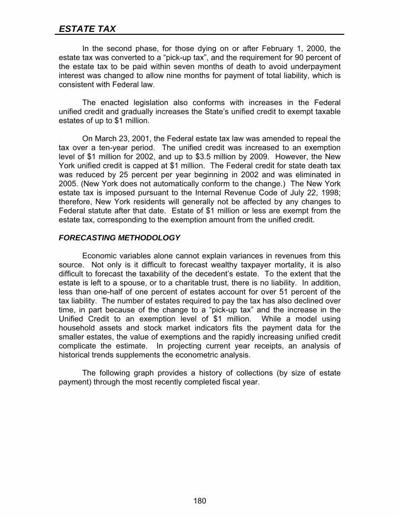
ESTATE TAX
180
In the second phase, for those dying on or after February 1, 2000, the estate tax was converted to a “pick-up tax”, and the requirement for 90 percent of the estate tax to be paid within seven months of death to avoid underpayment interest was changed to allow nine months for payment of total liability, which is consistent with Federal law. The enacted legislation also conforms with increases in the Federal unified credit and gradually increases the State’s unified credit to exempt taxable estates of up to $1 million. On March 23, 2001, the Federal estate tax law was amended to repeal the tax over a ten-year period. The unified credit was increased to an exemption level of $1 million for 2002, and up to $3.5 million by 2009. However, the New York unified credit is capped at $1 million. The Federal credit for state death tax was reduced by 25 percent per year beginning in 2002 and was eliminated in 2005. (New York does not automatically conform to the change.) The New York estate tax is imposed pursuant to the Internal Revenue Code of July 22, 1998; therefore, New York residents will generally not be affected by any changes to Federal statute after that date. Estate of $1 million or less are exempt from the estate tax, corresponding to the exemption amount from the unified credit. FORECASTING METHODOLOGY Economic variables alone cannot explain variances in revenues from this source. Not only is it difficult to forecast wealthy taxpayer mortality, it is also difficult to forecast the taxability of the decedent’s estate. To the extent that the estate is left to a spouse, or to a charitable trust, there is no liability. In addition, less than one-half of one percent of estates account for over 51 percent of the tax liability. The number of estates required to pay the tax has also declined over time, in part because of the change to a “pick-up tax” and the increase in the Unified Credit to an exemption level of $1 million. While a model using household assets and stock market indicators fits the payment data for the smaller estates, the value of exemptions and the rapidly increasing unified credit complicate the estimate. In projecting current year receipts, an analysis of historical trends supplements the econometric analysis. The following graph provides a history of collections (by size of estate payment) through the most recently completed fiscal year.
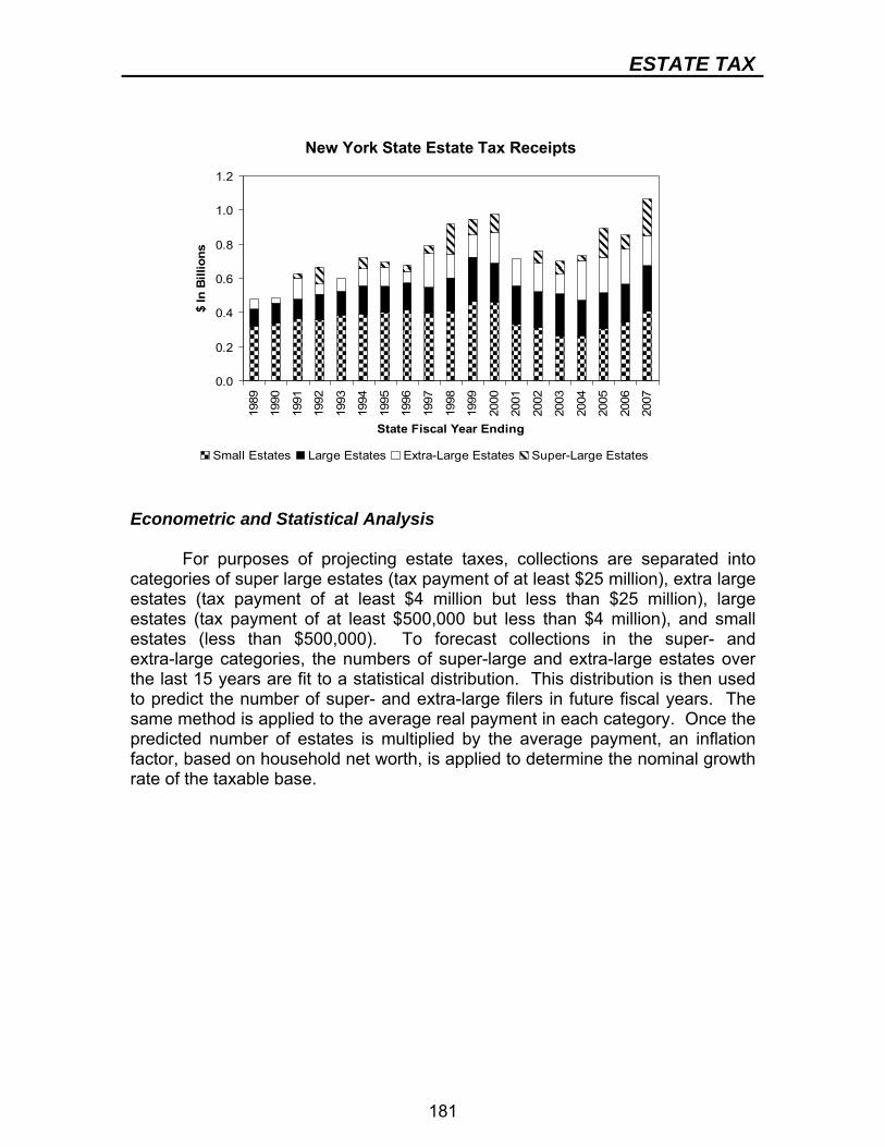
ESTATE TAX
181
New York State Estate Tax Receipts
0.0
0.2
0.4
0.6
0.8
1.0
1.2
1989
1990
1991
1992
1993
1994
1995
1996
1997
1998
1999
2000
2001
2002
2003
2004
2005
2006
2007
State Fiscal Year Ending
$ In
Bill
ions
Small Estates Large Estates Extra-Large Estates Super-Large Estates
Econometric and Statistical Analysis For purposes of projecting estate taxes, collections are separated into categories of super large estates (tax payment of at least $25 million), extra large estates (tax payment of at least $4 million but less than $25 million), large estates (tax payment of at least $500,000 but less than $4 million), and small estates (less than $500,000). To forecast collections in the super- and extra-large categories, the numbers of super-large and extra-large estates over the last 15 years are fit to a statistical distribution. This distribution is then used to predict the number of super- and extra-large filers in future fiscal years. The same method is applied to the average real payment in each category. Once the predicted number of estates is multiplied by the average payment, an inflation factor, based on household net worth, is applied to determine the nominal growth rate of the taxable base.
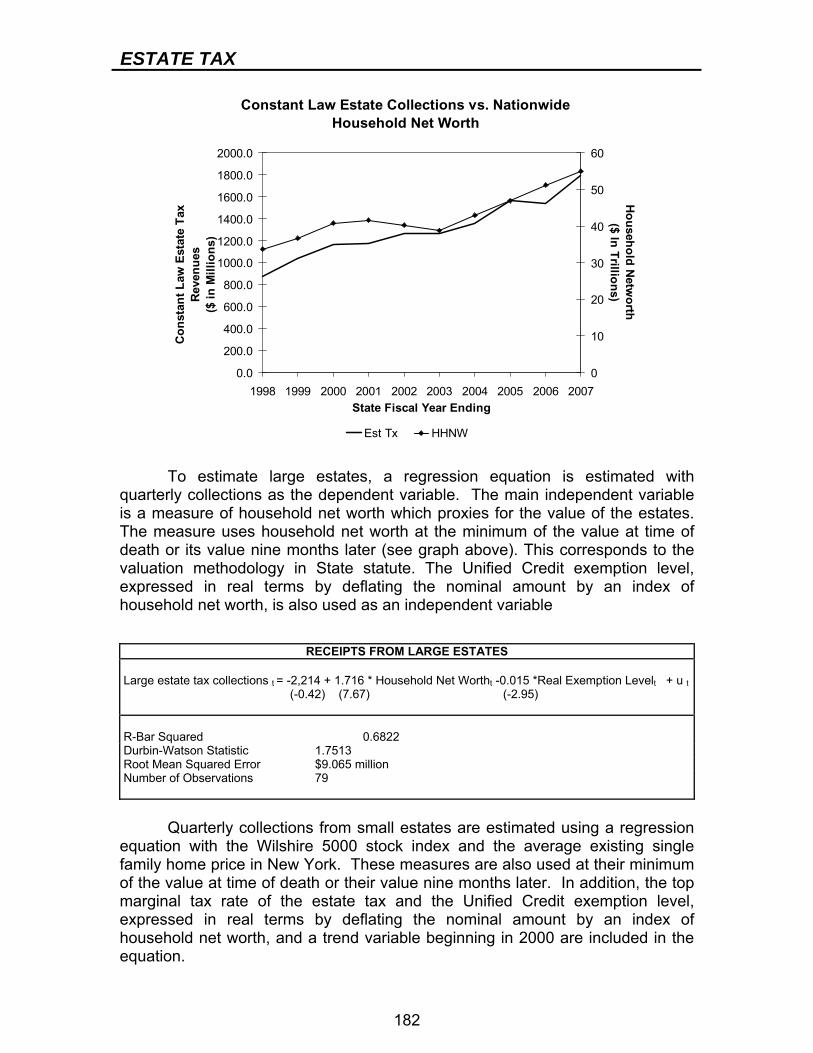
ESTATE TAX
182
Constant Law Estate Collections vs. Nationwide Household Net Worth
0.0
200.0
400.0
600.0
800.0
1000.0
1200.0
1400.0
1600.0
1800.0
2000.0
1998 1999 2000 2001 2002 2003 2004 2005 2006 2007State Fiscal Year Ending
Con
stan
t Law
Est
ate
Tax
Rev
enue
s($
in M
illio
ns)
0
10
20
30
40
50
60
Household N
etworth
($ In Trillions)
Est Tx HHNW
To estimate large estates, a regression equation is estimated with quarterly collections as the dependent variable. The main independent variable is a measure of household net worth which proxies for the value of the estates. The measure uses household net worth at the minimum of the value at time of death or its value nine months later (see graph above). This corresponds to the valuation methodology in State statute. The Unified Credit exemption level, expressed in real terms by deflating the nominal amount by an index of household net worth, is also used as an independent variable
Quarterly collections from small estates are estimated using a regression equation with the Wilshire 5000 stock index and the average existing single family home price in New York. These measures are also used at their minimum of the value at time of death or their value nine months later. In addition, the top marginal tax rate of the estate tax and the Unified Credit exemption level, expressed in real terms by deflating the nominal amount by an index of household net worth, and a trend variable beginning in 2000 are included in the equation.
RECEIPTS FROM LARGE ESTATES Large estate tax collections t = -2,214 + 1.716 * Household Net Wortht -0.015 *Real Exemption Levelt + u t (-0.42) (7.67) (-2.95) R-Bar Squared 0.6822 Durbin-Watson Statistic 1.7513 Root Mean Squared Error $9.065 million Number of Observations 79
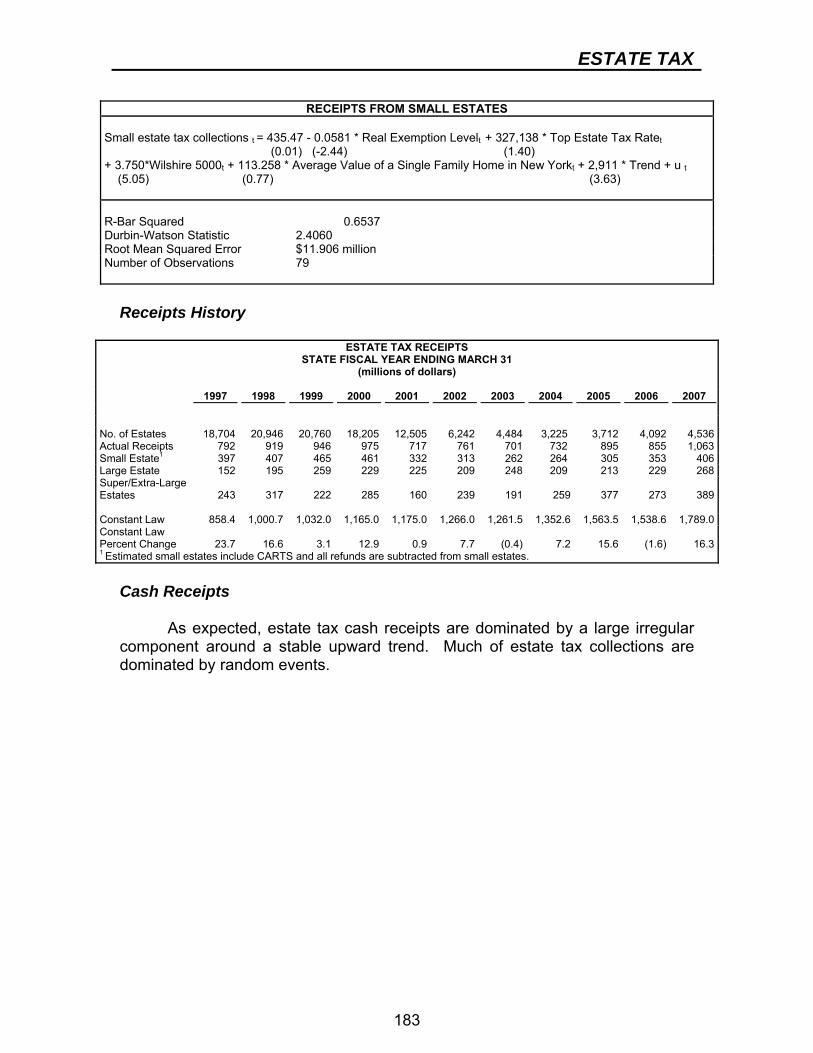
ESTATE TAX
183
Receipts History
ESTATE TAX RECEIPTS STATE FISCAL YEAR ENDING MARCH 31
(millions of dollars)
1997 1998 1999 2000 2001 2002 2003 2004 2005 2006 2007 No. of Estates 18,704 20,946 20,760 18,205 12,505 6,242 4,484 3,225 3,712 4,092 4,536Actual Receipts 792 919 946 975 717 761 701 732 895 855 1,063Small Estate1 397 407 465 461 332 313 262 264 305 353 406Large Estate 152 195 259 229 225 209 248 209 213 229 268Super/Extra-Large Estates 243 317 222 285 160 239 191 259 377 273 389 Constant Law 858.4 1,000.7 1,032.0 1,165.0 1,175.0 1,266.0 1,261.5 1,352.6 1,563.5 1,538.6 1,789.0 Constant Law Percent Change 23.7 16.6 3.1 12.9 0.9 7.7 (0.4) 7.2 15.6 (1.6) 16.31 Estimated small estates include CARTS and all refunds are subtracted from small estates.
Cash Receipts As expected, estate tax cash receipts are dominated by a large irregular component around a stable upward trend. Much of estate tax collections are dominated by random events.
RECEIPTS FROM SMALL ESTATES Small estate tax collections t = 435.47 - 0.0581 * Real Exemption Levelt + 327,138 * Top Estate Tax Ratet (0.01) (-2.44) (1.40) + 3.750*Wilshire 5000t + 113.258 * Average Value of a Single Family Home in New Yorkt + 2,911 * Trend + u t (5.05) (0.77) (3.63) R-Bar Squared 0.6537 Durbin-Watson Statistic 2.4060 Root Mean Squared Error $11.906 million Number of Observations 79
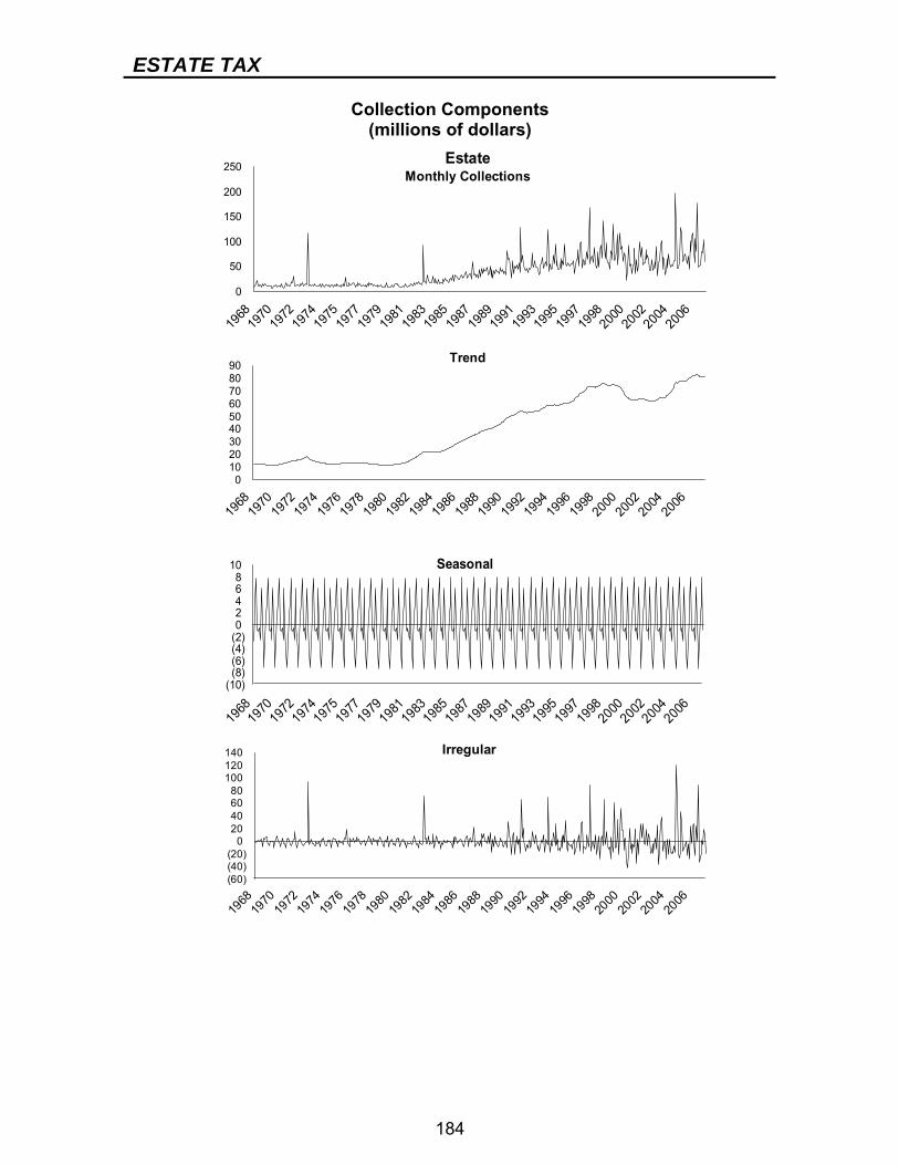
ESTATE TAX
184
Collection Components (millions of dollars)
0
50
100
150
200
250
1968
1970
1972
1974
1975
1977
1979
1981
1983
1985
1987
1989
1991
1993
1995
1997
1998
2000
2002
2004
2006
EstateMonthly Collections
0102030405060708090
1968
1970
1972
1974
1976
1978
1980
1982
1984
1986
1988
1990
1992
1994
1996
1998
2000
2002
2004
2006
Trend
(10)(8)(6)(4)(2)02468
10
1968
1970
1972
1974
1975
1977
1979
1981
1983
1985
1987
1989
1991
199319
9519
9719
9820
0020
02200
420
06
Seasonal
(60)(40)(20)
020406080
100120140
1968
1970
1972
1974
1976
1978
1980
1982
1984
1986
1988
1990
1992
1994
1996
1998
2000
2002
2004
2006
Irregular
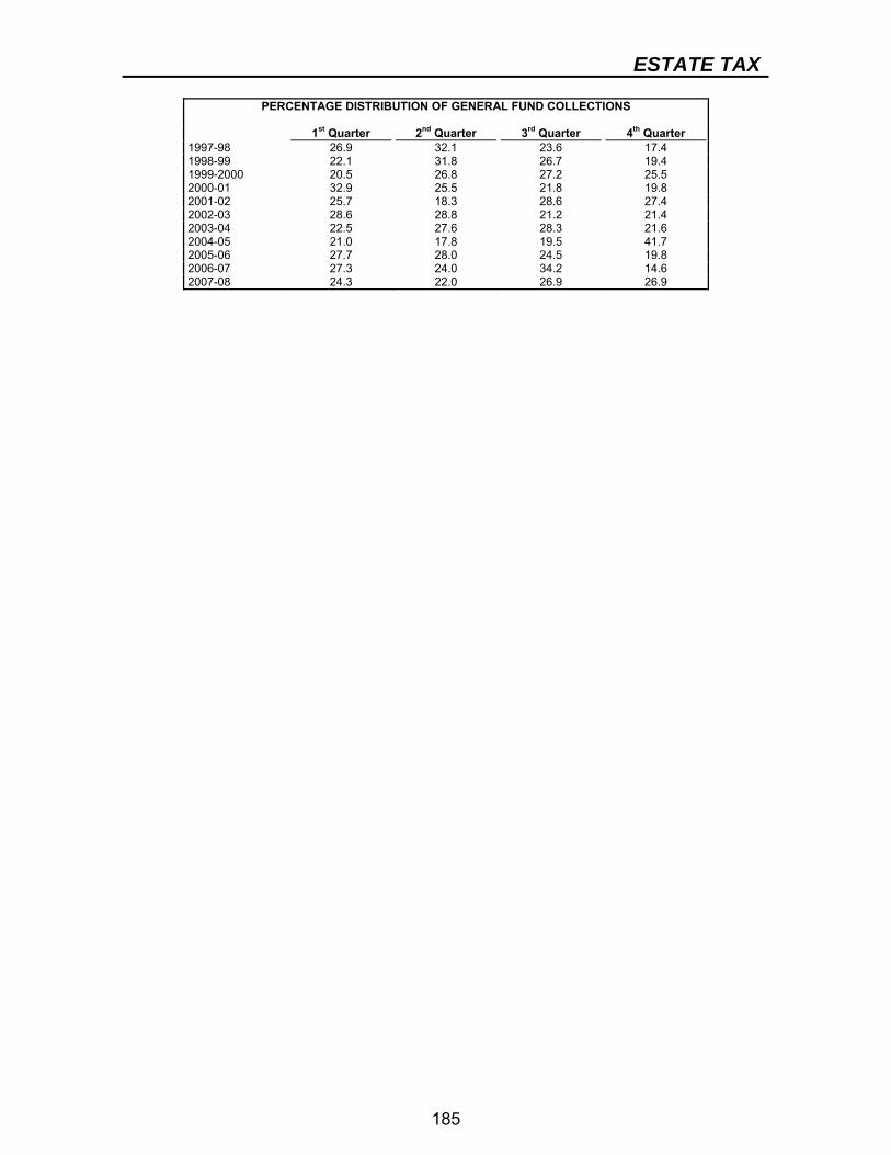
ESTATE TAX
185
PERCENTAGE DISTRIBUTION OF GENERAL FUND COLLECTIONS
1st Quarter 2nd Quarter 3rd Quarter 4th Quarter 1997-98 26.9 32.1 23.6 17.4 1998-99 22.1 31.8 26.7 19.4 1999-2000 20.5 26.8 27.2 25.5 2000-01 32.9 25.5 21.8 19.8 2001-02 25.7 18.3 28.6 27.4 2002-03 28.6 28.8 21.2 21.4 2003-04 22.5 27.6 28.3 21.6 2004-05 21.0 17.8 19.5 41.7 2005-06 27.7 28.0 24.5 19.8 2006-07 27.3 24.0 34.2 14.6 2007-08 24.3 22.0 26.9 26.9
186
REAL ESTATE TRANSFER TAX BACKGROUND Tax Base and Rate The New York State real estate transfer tax (RETT) is imposed on each conveyance of real property or interest therein when the consideration exceeds $500, at a rate of $4.00 per $1,000 of consideration. The tax became effective August 1, 1968. Prior to May 1983, the rate was $1.10 per $1,000 of consideration. An additional “mansion” tax, effective July 1, 1989, is imposed on conveyances of residential real property for which the consideration is $1 million or more at a rate of 1 percent of the total consideration attributable to residential property. The tax rate imposed on conveyances into new or existing real estate investment trusts (REITS) is $2.00 per $1,000 of consideration. For deeded transfers, the tax is paid to a recording agent (generally the county clerk). For non-deeded transactions, payments are made directly to the Commissioner of the Department of Taxation and Finance. All payments are due within 15 days of the transfer. For counties that had more than $1.2 million in liability during the previous calendar year, payments received between the first and fifteenth day of the month are due to the Commissioner by the twenty-fifth day of the same month. Payments received in such counties between the sixteenth and final day of the month are due to the Commissioner by the tenth day of the following month. Payments from all other counties are due to the commissioner by the tenth day of the month following their receipt. DATA SOURCES The primary sources of data used in the estimation and forecasting methodology for the RETT are as follows:
● AMO43, Department of Taxation and Finance Monthly Report of Receipts. This report contains gross and net receipts data.
● RETT 7, Department of Taxation and Finance. This form reports the monthly liability for each county. It is an important source of information, since some counties do not remit payments to the Commissioner according to the statutory schedule.
● Various U.S., New York State and New York City government agencies, including the U.S. Bureau of Economic Analysis of the Commerce Department. These agencies provide economic data used in the econometric equation.
● Various real estate industry sources including : National Association of Realtors, CB Richard Ellis (vacancy rates), Prudential Douglas Ellison Real Estate (Market Reports); and the Furman Center for Real Estate and Urban Policy at NYU School of Law.

REAL ESTATE TRANSFER TAX
187
FORECAST METHODOLOGY Real estate transfer tax collections are dependent on the total value of real estate conveyances, which in turn are a function of the number of conveyances and the price of each individual conveyance. Between 55 percent and 65 percent of monthly collections are the result of activity in New York City and Long Island. Real estate values and the number of transfers in this geographical area are subject to more cyclical behavior than in the remainder of the State. This is due to the nature of the local economy, which is more dependent on financial services than the remainder of the State and the nation as a whole, and to the sometimes speculative nature of expected returns on commercial real estate transactions. A regression equation is estimated with fiscal year liability (excluding the mansion tax) divided by the tax rate, which yields the dollar value of transfers, as the dependent variable. Independent variables in the model are: the mortgage rate, New York housing starts multiplied by an average New York housing price which yields a “value of sold housing” variable, Manhattan vacancy rates, and the national price deflator for nonresidential construction (buildings and other). Mansion tax receipts are estimated using a separate equation, in which the average New York housing price is the primary independent variable. A dummy captures the large increase in collections in SFY 2001-02. As the fiscal year progresses, year-to-date collections and liability are additional factors that determine the current-year estimate. The period of actual observations is SFY 1974-75 to 2006-07.
RETT (NON-MANSION TAX EQUATION) Dollar Value of Transfers = -21,556.7 – 1,373.37*[mortgage rate] + .0058*[value of sold housing] + (-1.22) (-1.44) (4.52) 79,320*[U.S. construction deflator, buildings] - 15.41*[square of Manhattan vacancy rates] (4.52) (-2.65) R-Bar Squared 0.9391 Durbin-Watson Statistic 0.4998 Standard Error of the Regression* $17.7 million Number of Observations 33 *Normalized
RETT (MANSION TAX EQUATION) Mansion Tax Receipts = -154.1 + 1.25*[avg house price] + 19.34*[Dummy for SFY 2001 Increase] (-12.31) (19.34) (0.92) R-Bar Squared 0.9665 Durbin-Watson Statistic 0.6140 Standard Error of the Regression $12.5 million Number of Observations 17
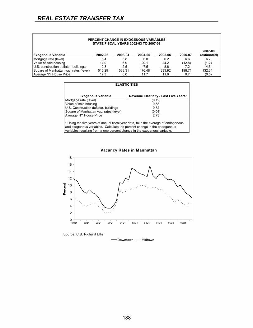
REAL ESTATE TRANSFER TAX
188
PERCENT CHANGE IN EXOGENOUS VARIABLES STATE FISCAL YEARS 2002-03 TO 2007-08
2007-08 Exogenous Variable 2002-03 2003-04 2004-05 2005-06 2006-07 (estimated) Mortgage rate (level) 6.4 5.8 6.0 6.2 6.6 6.7 Value of sold housing 14.0 6.9 20.1 24.2 (12.8) (1.2) U.S. construction deflator, buildings 2.8 2.5 7.5 8.6 7.2 4.3 Square of Manhattan vac. rates (level) 515.29 538.31 476.48 333.92 198.71 132.34 Average NY House Price 12.3 6.0 11.7 11.9 0.7 (0.5)
ELASTICITIES
Exogenous Variable Revenue Elasticity - Last Five Years* Mortgage rate (level) (0.12) Value of sold housing 0.53 U.S. Construction deflator, buildings 0.82 Square of Manhattan vac. rates (level) (0.04) Average NY House Price 2.73 * Using the five years of annual fiscal year data, take the average of endogenous and exogenous variables. Calculate the percent change in the endogenous variables resulting from a one percent change in the exogenous variable.
Vacancy Rates in Manhattan
0
2
4
6
8
10
12
14
16
18
97Q4 98Q4 99Q4 00Q4 01Q4 02Q4 03Q4 04Q4 05Q4 06Q4
Perc
ent
Downtown Midtown
Source: C.B. Richard Ellis

REAL ESTATE TRANSFER TAX
189
Risks to the Forecast Errors in the forecasts of the exogenous variables provide a degree of risk to the real estate transfer tax forecast. Forecast error in prior years can largely be attributed to the forecasts of the exogenous variables and large unanticipated transfers. Variation in the estimate may also occur as a result of administrative changes or unanticipated legislative action. Cash Receipts The accelerating trend in collections in recent years is significant and large irregular values relative to trend indicate the significant volatility in this series. The typical payment behavior of all counties is used to estimate State cash receipts.
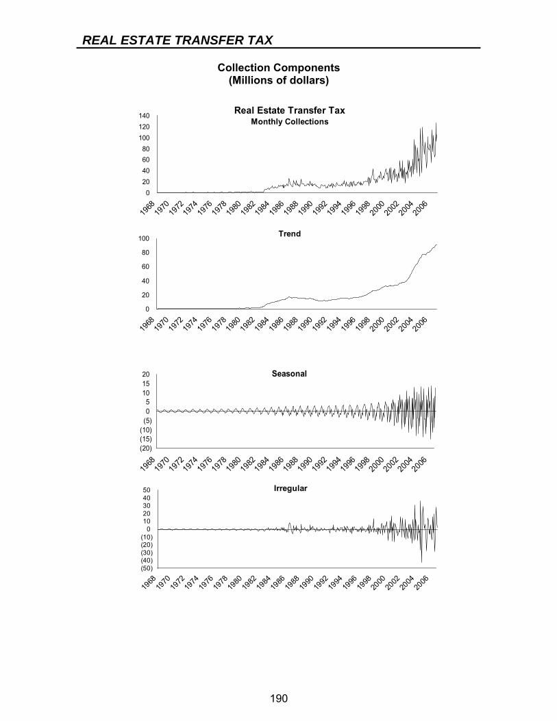
REAL ESTATE TRANSFER TAX
190
Collection Components (Millions of dollars)
020406080
100120140
1968
1970
1972
1974
1976
1978
1980
1982
1984
1986
1988
1990
1992
1994
1996
1998
2000
2002
2004
2006
Real Estate Transfer TaxMonthly Collections
0
20
40
60
80
100
1968
1970
1972
1974
1976
1978
1980
1982
1984
1986
1988
1990
1992
1994
1996
1998
2000
2002
2004
2006
Trend
(20)(15)(10)(5)05
101520
1968
1970
1972
1974
1976
1978
1980
1982
1984
1986
1988
1990
1992
1994
1996
1998
2000
2002
2004
2006
Seasonal
(50)(40)(30)(20)(10)
01020304050
1968
1970
1972
1974
1976
1978
1980
1982
1984
1986
1988
1990
1992
1994
1996
1998
2000
2002
2004
2006
Irregular
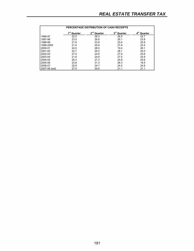
REAL ESTATE TRANSFER TAX
191
PERCENTAGE DISTRIBUTION OF CASH RECEIPTS
1st Quarter 2nd Quarter 3rd Quarter 4th Quarter 1996-97 22.5 28.3 26.5 22.7 1997-98 23.5 26.6 26.1 23.8 1998-99 21.9 33.9 23.4 20.8 1999-2000 21.0 25.8 27.8 25.4 2000-01 24.5 28.0 19.4 28.1 2001-02 22.7 29.2 28.1 20.0 2002-03 27.0 24.8 27.6 20.6 2003-04 21.8 24.8 27.5 25.9 2004-05 26.3 27.3 25.8 20.6 2005-06 23.8 31.3 26.3 18.5 2006-07 25.9 24.7 24.5 24.8 2007-08 (est) 27.0 30.6 21.1 21.1
192
PARI-MUTUEL TAXES TAX BASE AND RATE Since 1940, the pari-mutuel tax has been levied on pari-mutuel wagering activity, conducted first at horse racetracks and later at simulcast theaters and off-track betting (OTB) parlors throughout the State. Each racing association or corporation pays the State a portion of the commission (the “takeout”) withheld from wagering pools (the “handle”) as a tax for the privilege of conducting pari-mutuel wagering on horse races. In general, the tax varies based on the type of racing (thoroughbred or harness), the place where the bet is made (on-track or off-track), and the type of wager (regular, multiple, or exotic). In the 1980s, the on-track harness handle was over $850 million and the effective tax rate was over 8 percent. Currently, the on-track and simulcast handle at harness tracks is marginally over $90 million, with an effective tax rate of 1.1 percent. Similarly, the on-track and simulcast thoroughbred handle has fallen from over $800 million to less than $450 million and its effective tax rate from over 9 percent to 1.5 percent. Off-track betting, which started in 1972, had rapid growth in the 1970s and 1980s, as new facilities came on line and the State increased the hours of operation and types of betting. The handle at OTB's has grown to over $2.0 billion, and its effective tax rate was reduced from over 3 percent to 0.7 percent. ADMINISTRATION The tax is collected by each on-track and off-track racing association, or corporation, and remitted to the State Commissioner of Taxation and Finance each month on the last business day. Such taxes cover the liability due for the period from the 16th day of the preceding month through the 15th day of the current month. DATA SOURCES Data on the pari-mutuel tax come from various sources:
● AM043 Department of Taxation and Finance. Monthly reports containing collection data.
● OTB and Racetracks. Monthly reports are collected from OTB and various racetracks provide data upon request.
● New York State Racing and Wagering Board. The Board provides annual reports and additional information upon request.
● Office of the State Comptroller. Monthly reports containing collection data. STATUTORY CHANGES Over the last two decades, increases in OTB activity and simulcasts, which now account for nearly 80 percent of the statewide handle, have been
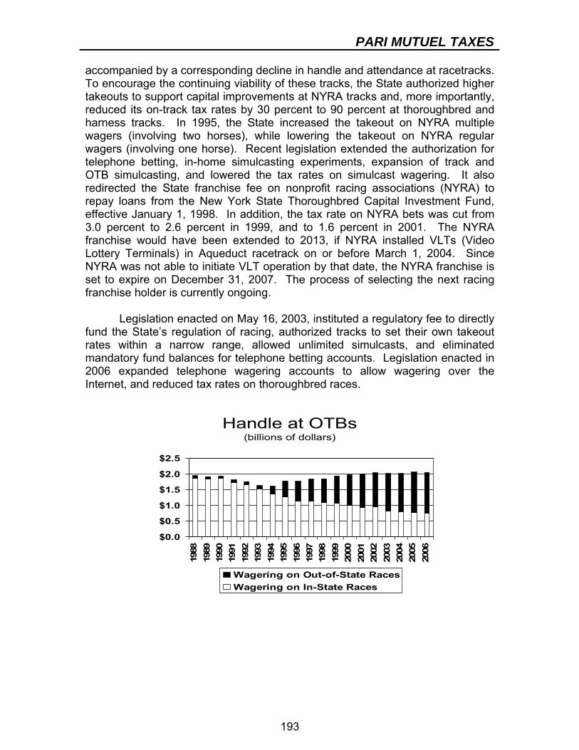
PARI MUTUEL TAXES
193
accompanied by a corresponding decline in handle and attendance at racetracks. To encourage the continuing viability of these tracks, the State authorized higher takeouts to support capital improvements at NYRA tracks and, more importantly, reduced its on-track tax rates by 30 percent to 90 percent at thoroughbred and harness tracks. In 1995, the State increased the takeout on NYRA multiple wagers (involving two horses), while lowering the takeout on NYRA regular wagers (involving one horse). Recent legislation extended the authorization for telephone betting, in-home simulcasting experiments, expansion of track and OTB simulcasting, and lowered the tax rates on simulcast wagering. It also redirected the State franchise fee on nonprofit racing associations (NYRA) to repay loans from the New York State Thoroughbred Capital Investment Fund, effective January 1, 1998. In addition, the tax rate on NYRA bets was cut from 3.0 percent to 2.6 percent in 1999, and to 1.6 percent in 2001. The NYRA franchise would have been extended to 2013, if NYRA installed VLTs (Video Lottery Terminals) in Aqueduct racetrack on or before March 1, 2004. Since NYRA was not able to initiate VLT operation by that date, the NYRA franchise is set to expire on December 31, 2007. The process of selecting the next racing franchise holder is currently ongoing. Legislation enacted on May 16, 2003, instituted a regulatory fee to directly fund the State’s regulation of racing, authorized tracks to set their own takeout rates within a narrow range, allowed unlimited simulcasts, and eliminated mandatory fund balances for telephone betting accounts. Legislation enacted in 2006 expanded telephone wagering accounts to allow wagering over the Internet, and reduced tax rates on thoroughbred races.
Handle at OTBs(billions of dollars)
$0.0
$0.5
$1.0
$1.5
$2.0
$2.5
1988
1989
1990
1991
1992
1993
1994
1995
1996
1997
1998
1999
2000
2001
2002
2003
2004
2005
2006
Wagering on Out-of-State RacesWagering on In-State Races
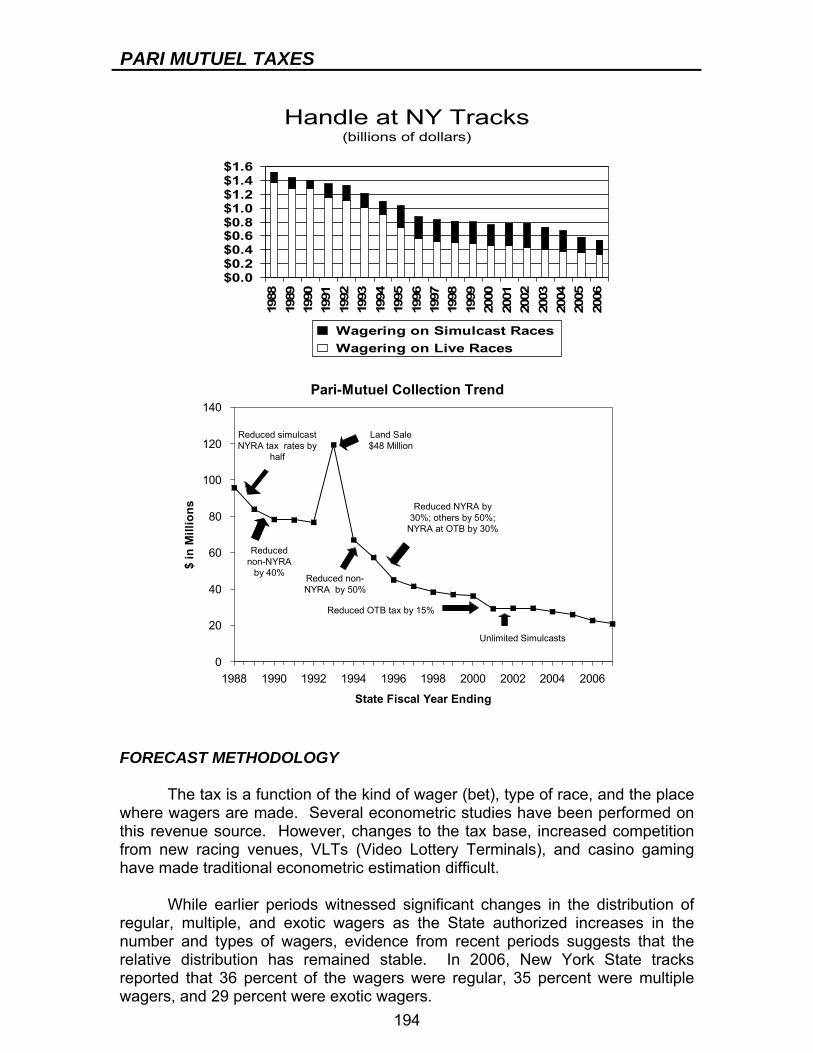
PARI MUTUEL TAXES
194
Handle at NY Tracks(billions of dollars)
$0.0$0.2$0.4$0.6$0.8$1.0$1.2$1.4$1.6
1988
1989
1990
1991
1992
1993
1994
1995
1996
1997
1998
1999
2000
2001
2002
2003
2004
2005
2006
Wagering on Simulcast Races Wagering on Live Races
Pari-Mutuel Collection Trend
0
20
40
60
80
100
120
140
1988 1990 1992 1994 1996 1998 2000 2002 2004 2006
State Fiscal Year Ending
$ in
Mill
ions
Reduced simulcast NYRA tax rates by
half
Reduced non-NYRA
by 40% Reduced non-NYRA by 50%
Land Sale $48 Million
Reduced NYRA by 30%; others by 50%;
NYRA at OTB by 30%
Reduced OTB tax by 15%
Unlimited Simulcasts
FORECAST METHODOLOGY The tax is a function of the kind of wager (bet), type of race, and the place where wagers are made. Several econometric studies have been performed on this revenue source. However, changes to the tax base, increased competition from new racing venues, VLTs (Video Lottery Terminals), and casino gaming have made traditional econometric estimation difficult. While earlier periods witnessed significant changes in the distribution of regular, multiple, and exotic wagers as the State authorized increases in the number and types of wagers, evidence from recent periods suggests that the relative distribution has remained stable. In 2006, New York State tracks reported that 36 percent of the wagers were regular, 35 percent were multiple wagers, and 29 percent were exotic wagers.
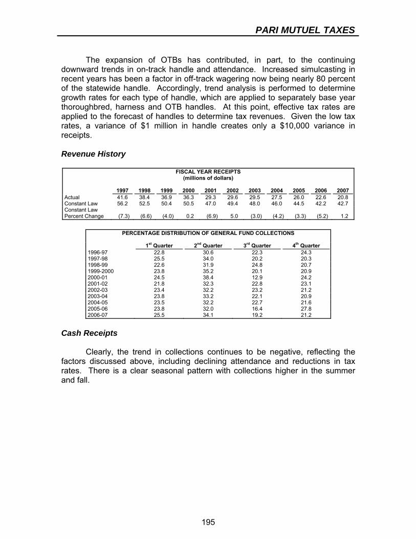
PARI MUTUEL TAXES
195
The expansion of OTBs has contributed, in part, to the continuing downward trends in on-track handle and attendance. Increased simulcasting in recent years has been a factor in off-track wagering now being nearly 80 percent of the statewide handle. Accordingly, trend analysis is performed to determine growth rates for each type of handle, which are applied to separately base year thoroughbred, harness and OTB handles. At this point, effective tax rates are applied to the forecast of handles to determine tax revenues. Given the low tax rates, a variance of $1 million in handle creates only a $10,000 variance in receipts. Revenue History
PERCENTAGE DISTRIBUTION OF GENERAL FUND COLLECTIONS
1st Quarter 2nd Quarter 3rd Quarter 4th Quarter 1996-97 22.8 30.6 22.3 24.3 1997-98 25.5 34.0 20.2 20.3 1998-99 22.6 31.9 24.8 20.7 1999-2000 23.8 35.2 20.1 20.9 2000-01 24.5 38.4 12.9 24.2 2001-02 21.8 32.3 22.8 23.1 2002-03 23.4 32.2 23.2 21.2 2003-04 23.8 33.2 22.1 20.9 2004-05 23.5 32.2 22.7 21.6 2005-06 23.8 32.0 16.4 27.8 2006-07 25.5 34.1 19.2 21.2
Cash Receipts Clearly, the trend in collections continues to be negative, reflecting the factors discussed above, including declining attendance and reductions in tax rates. There is a clear seasonal pattern with collections higher in the summer and fall.
FISCAL YEAR RECEIPTS (millions of dollars)
1997 1998 1999 2000 2001 2002 2003 2004 2005 2006 2007 Actual 41.6 38.4 36.9 36.3 29.3 29.6 29.5 27.5 26.0 22.6 20.8 Constant Law 56.2 52.5 50.4 50.5 47.0 49.4 48.0 46.0 44.5 42.2 42.7 Constant Law Percent Change
(7.3)
(6.6)
(4.0)
0.2
(6.9)
5.0
(3.0)
(4.2)
(3.3)
(5.2)
1.2
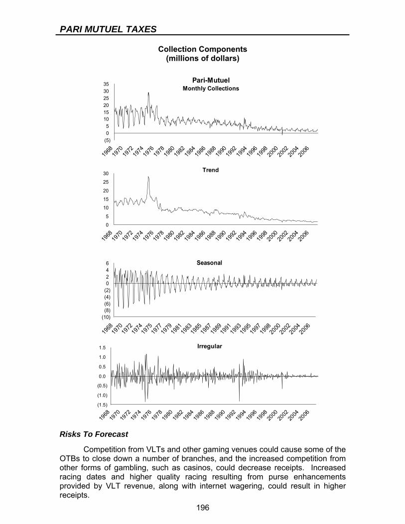
PARI MUTUEL TAXES
196
Collection Components (millions of dollars)
(5)05
101520253035
1968
1970
1972
1974
1976
1978
1980
1982
1984
1986
1988
1990
1992
1994
1996
1998
2000
2002
2004
2006
Pari-Mutuel Monthly Collections
0
5
10
15
20
25
30
1968
1970
1972
1974
1976
1978
1980
1982
1984
1986
1988
1990
1992
1994
1996
1998
2000
2002
2004
2006
Trend
(10)(8)(6)(4)(2)0246
1968
1970
1972
1974
1975
1977
1979
1981
1983
1985
1987
1989
1991
199319
9519
9719
9820
0020
02200
420
06
Seasonal
(1.5)
(1.0)
(0.5)
0.0
0.5
1.0
1.5
1968
1970
1972
1974
1976
1978
1980
1982
1984
1986
1988
1990
1992
1994
1996
1998
2000
2002
2004
2006
Irregular
Risks To Forecast Competition from VLTs and other gaming venues could cause some of the OTBs to close down a number of branches, and the increased competition from other forms of gambling, such as casinos, could decrease receipts. Increased racing dates and higher quality racing resulting from purse enhancements provided by VLT revenue, along with internet wagering, could result in higher receipts.


198
LOTTERY TAX BASE AND RATE In 1966, New York State voters approved a referendum authorizing a State lottery, and ticket sales commenced under the auspices of the Lottery Commission. Under the original lottery legislation, a lotto-type game was offered with 12 drawings a year, 30 percent of gross receipts earmarked to prizes, 55 percent to education, and the remaining 15 percent representing an upper limit on administrative expenses. Since its inception, numerous games have been introduced with varying prize payout schedules to make them attractive to the consumer. In 1973, the New York State Racing and Wagering Board took over operation of the Lottery from the Lottery Commission. The New York State Division of the Lottery was established in 1976, and assumed the operation of the State's Lottery. The Lottery Division, as an independent agency within the Department of Taxation and Finance, manages the operation and sales of the State's Lottery games. The Lottery Division is authorized to operate five types of games:
1. Instant games, sold as scratch-off tickets in which most prizes are won immediately (approximately 60 games are currently being offered for sale with prices ranging from $1 to $20);
2. Lotto games, which are pari-mutuel, pick-your-own-numbers games offering large top prizes, with drawings conducted 11 times weekly: seven 5-of-39 draws (Take-5), two 6-of-59 draws (Lotto 59) and two multi-jurisdictional drawings (Mega Millions). For the Lotto 59 game and the Mega Millions game, the value of any top prize not won is added to the top prize in the subsequent drawing;
3. Daily numbers games, which are fixed-odds games, with two daily drawings where players select either a three-digit number (Daily Numbers), or a four-digit number (Win 4), and Instant Win, an add-on game to Daily Numbers and Win 4;
4. Keno-like games, which are pari-mutuel pick-your-own 10-of-80 numbers games, with drawings conducted either daily (Pick 10) or every four minutes (Quick Draw) during certain intervals. The Lottery Division pays top prizes of $500,000 in Pick 10 and $100,000 in Quick Draw; and
5. Video lottery games, which are lottery games played on video gaming devices. Video Lottery Terminals (VLTs) are currently authorized only at selected thoroughbred and harness tracks.
The Comptroller, pursuant to an appropriation, distributes all net receipts from the lottery directly to school districts for the purposes of providing school aid. This aid also provides special allowances for textbooks for all school children and additional amounts for pupils in approved State-supported schools for the deaf and the blind. The statutory allocation for education for Lotto 59 and Instant Win games is 45 percent of ticket sales; for Take 5, Mega Millions, Daily Numbers, Win 4, and Pick 10 games, 35 percent; for Instant games, 20 percent and 10 percent for

LOTTERY
199
up to three Instant Games per year; for Quick Draw, 25 percent. The Lottery Division sets aside 15 percent of revenue from sales all traditional lottery games for its administration, and the remainder is available to support education. At the end of each fiscal year, any unspent portion of the 15 percent of ticket sales not used for administration is also used for education. The remaining portion of sales revenue is used to pay prizes. For the Video Lottery program, prizes of not less than 90 percent of sales are paid out to determine net machine income (NMI). The NMI is distributed based on graduated schedules with an allocation ranging from 50 percent to 60 percent of net machine income for education, depending on the net machine income of each facility. The Lottery Division retains 10 percent of NMI for administration of the program, with the host racetracks retaining the remaining portion of NMI as a commission. ADMINISTRATION Sales agents are notified electronically by the Lottery Division’s lottery game vendor by Monday of each week of the amount due the State from sales during the previous week. The agent has until Tuesday to deposit sufficient funds in specified joint bank accounts at which time the operations vendor sweeps the moneys and transfers them to the Lottery Division by Wednesday morning. For VLTs, the Division sweeps the accounts daily and the State receives the revenues daily. DATA SOURCES Data is collected from the Division of the Lottery on a weekly and monthly basis. STATUTORY CHANGES Legislation enacted in 1987, 1988, 1991, and 1999 increased the prize allocation for Instant games from 45 percent, to 50 percent, to 55 percent, and finally to 65 percent, respectively. Legislation enacted in 1995 and renewed in 1999, 2001, 2002, 2004, 2005 and 2006 authorized the Quick Draw game through May 31, 2007. Legislation enacted on October 29, 2001, allowed the Lottery Division to enter into multi-jurisdictional agreements to conduct multistate lotto games with a 50 percent prize payout. The State elected to join with the Big Game states, and afterward the name was changed to Mega Millions. In addition, this 2001 legislation allowed the Lottery Division to license the operation of VLTs at selected New York State racetracks. Legislation enacted on January 28, 2002, allowed the Lottery Division to offer up to three 75 percent prize payout Instant ticket games during the fiscal year.

LOTTERY
200
Legislation enacted on April 12, 2005, made the following changes to the VLT program:
● Of the total revenue wagered after payout for prizes, 32 percent of the first $50 million, 29 percent of the next $100 million and 26 percent thereafter shall be paid to the operator of the track.
● In addition, the legislation provided for an additional vendor’s marketing allowance equal to 8 percent of the first $100 million and 5 percent thereafter of total revenue wagered after payout for prizes to be used by the vendor track for the marketing and promotion and associated costs of its operations provided, however, that the allowance shall not exceed 4 percent in any year for a racetrack located in the county of Westchester or Queens.
● The 10 percent of total revenue after payout for prizes used for the expenses of the Lottery Division was not changed in this legislation.
● By implication, of the total revenue wagered after payout for prizes, 54 percent of the first $50 million, 57 percent of the next $100 million and 60 percent thereafter is earmarked for education for tracks located in Westchester or Queens Counties, 50 percent of the first $50 million, 53 percent of the next $50 million and 56 percent of the next $50 million and 59 percent thereafter is earmarked for education from tracks not in Westchester or Queens counties.
● Extended the expiration of the program until December 31, 2017. FORECAST METHODOLOGY Economic conditions seem to have little explanatory power in predicting Lottery receipts. Accordingly, the various games are initially estimated using probability and time series models and are subsequently adjusted for marketing and operational plans, new game introductions, and law changes. Lotto and Mega Millions The sales of Lotto and Mega Millions tickets are volatile because the jackpots can randomly roll up to high amounts. High jackpots produce significant spikes in sales. The forecast of these games uses a simulation model that mimics the actual process and simulates one year of drawings. The model is run for 1,000 iterations (each iteration simulation one year of drawing) to produce output distributions for total sales, total revenue and the seeding necessary to maintain the jackpot levels. Distribution averages are used to predict the most likely receipts outcome. To run the model, the jackpot structure is input and then a regression model based on historical sales-to-jackpot relationships is used to obtain an estimate of the average sales at each jackpot level, correcting for seasonal effects and other factors. After the sales for a specific draw are calculated, another model predicts the average coverage ratio (the combinations actually bet divided by the total number of combinations) at that sales level.
LOTTERY
201
To determine if the jackpot will be hit, a random number generator is used to generate numbers between zero and one. If the random number is less than or equal to the coverage ratio, the jackpot is hit. If the random number is greater than the coverage ratio, the jackpot rolls to the next jackpot level and the model repeats the analysis. The model simulates 104 jackpot draws and thus one full year of results. Since the sales and coverage ratio are not the same every time a given jackpot level is drawn, the average sales and coverage ratio predicted by the regression equations cannot simply be used. Instead, a risk analysis program is used to substitute a probability distribution for sales at each jackpot level and a Latin Hypercube random selection process is used to pick the actual sales at every given jackpot level from the probability distribution. The probability distributions are based upon the historical variance in sales at various jackpot levels. To illustrate, sales of Lotto at a $3 million jackpot level may range between $2.5 million and $4.5 million, with an average of $3.5 million. The $3.5 million would be established using the regression equation and it can be postulated that the actual sales will vary according to a normal distribution with a mean of $3.5 million and a variance of $350,000. The risk analysis would randomly select the actual sales level from the distribution. The next time a $3 million jackpot is encountered, a different sales level would be selected which would produce a different coverage ratio. There are thousands of such distributions employed in the model. Performing the simulation 1,000 times essentially creates 1,000 potential years of results. This allows for the creation of distributions of possible results and evaluation of the probability of achieving a given level of sales. The model also contains features that allow the simulation of potential policy changes or other events that could affect sales, such as Mega Millions impact on Lotto, changing the size of the matrix, the interest rate, the level of seeding and altering the jackpot structure.
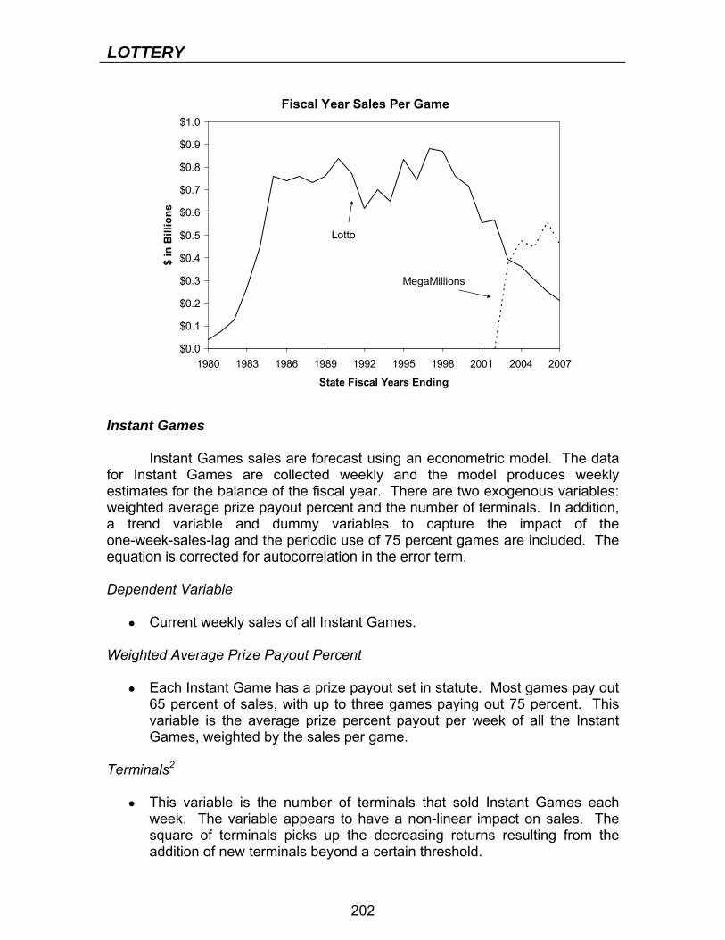
LOTTERY
202
Fiscal Year Sales Per Game
$0.0
$0.1
$0.2
$0.3
$0.4
$0.5
$0.6
$0.7
$0.8
$0.9
$1.0
1980 1983 1986 1989 1992 1995 1998 2001 2004 2007
State Fiscal Years Ending
$ in
Bill
ions
Lotto
MegaMillions
Instant Games Instant Games sales are forecast using an econometric model. The data for Instant Games are collected weekly and the model produces weekly estimates for the balance of the fiscal year. There are two exogenous variables: weighted average prize payout percent and the number of terminals. In addition, a trend variable and dummy variables to capture the impact of the one-week-sales-lag and the periodic use of 75 percent games are included. The equation is corrected for autocorrelation in the error term. Dependent Variable
● Current weekly sales of all Instant Games. Weighted Average Prize Payout Percent
● Each Instant Game has a prize payout set in statute. Most games pay out 65 percent of sales, with up to three games paying out 75 percent. This variable is the average prize percent payout per week of all the Instant Games, weighted by the sales per game.
Terminals2
● This variable is the number of terminals that sold Instant Games each
week. The variable appears to have a non-linear impact on sales. The square of terminals picks up the decreasing returns resulting from the addition of new terminals beyond a certain threshold.
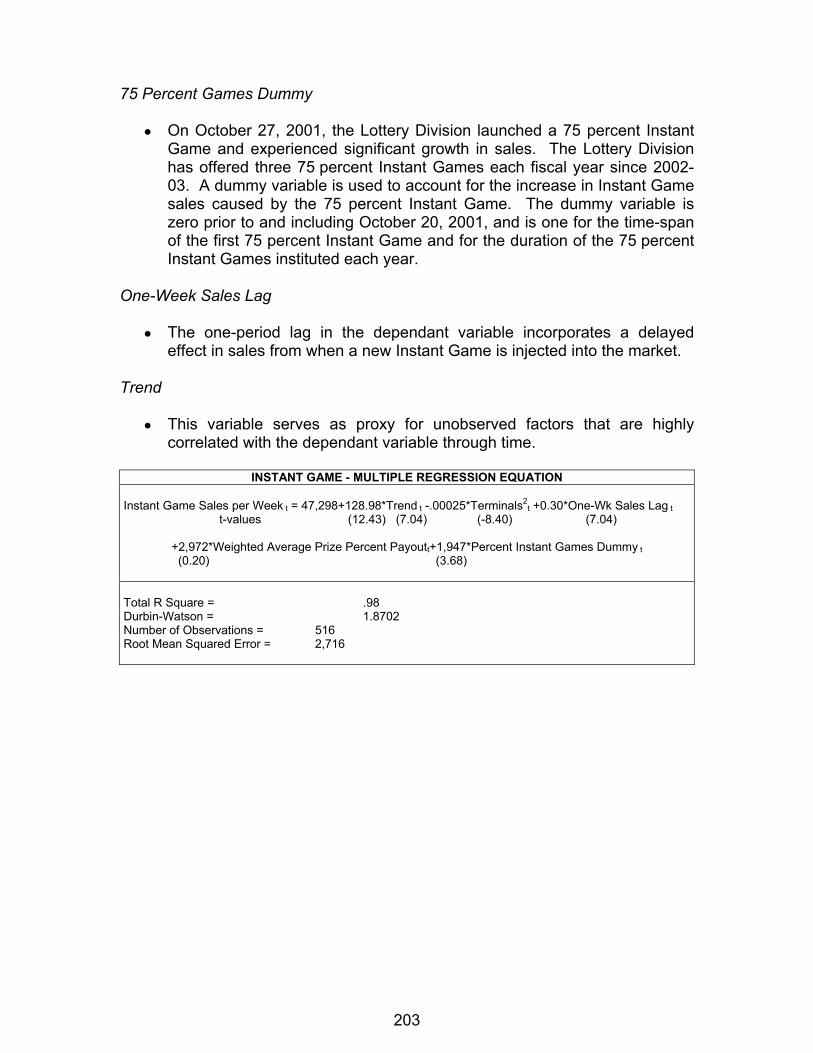
203
75 Percent Games Dummy
● On October 27, 2001, the Lottery Division launched a 75 percent Instant Game and experienced significant growth in sales. The Lottery Division has offered three 75 percent Instant Games each fiscal year since 2002-03. A dummy variable is used to account for the increase in Instant Game sales caused by the 75 percent Instant Game. The dummy variable is zero prior to and including October 20, 2001, and is one for the time-span of the first 75 percent Instant Game and for the duration of the 75 percent Instant Games instituted each year.
One-Week Sales Lag
● The one-period lag in the dependant variable incorporates a delayed effect in sales from when a new Instant Game is injected into the market.
Trend
● This variable serves as proxy for unobserved factors that are highly correlated with the dependant variable through time.
INSTANT GAME - MULTIPLE REGRESSION EQUATION
Instant Game Sales per Week t = 47,298+128.98*Trend t -.00025*Terminals2
t +0.30*One-Wk Sales Lag t t-values (12.43) (7.04) (-8.40) (7.04) +2,972*Weighted Average Prize Percent Payoutt+1,947*Percent Instant Games Dummy t (0.20) (3.68) Total R Square = .98 Durbin-Watson = 1.8702 Number of Observations = 516 Root Mean Squared Error = 2,716
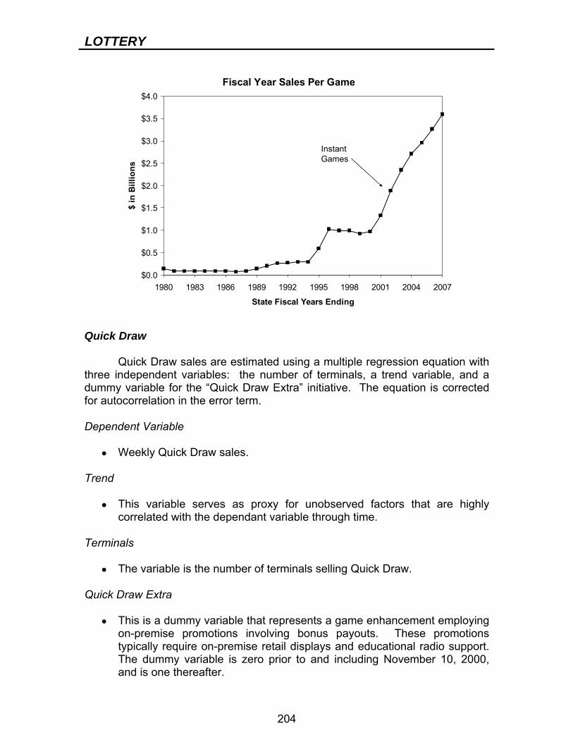
LOTTERY
204
Fiscal Year Sales Per Game
$0.0
$0.5
$1.0
$1.5
$2.0
$2.5
$3.0
$3.5
$4.0
1980 1983 1986 1989 1992 1995 1998 2001 2004 2007
State Fiscal Years Ending
$ in
Bill
ions
Instant Games
Quick Draw Quick Draw sales are estimated using a multiple regression equation with three independent variables: the number of terminals, a trend variable, and a dummy variable for the “Quick Draw Extra” initiative. The equation is corrected for autocorrelation in the error term. Dependent Variable
● Weekly Quick Draw sales. Trend
● This variable serves as proxy for unobserved factors that are highly correlated with the dependant variable through time.
Terminals
● The variable is the number of terminals selling Quick Draw. Quick Draw Extra
● This is a dummy variable that represents a game enhancement employing on-premise promotions involving bonus payouts. These promotions typically require on-premise retail displays and educational radio support. The dummy variable is zero prior to and including November 10, 2000, and is one thereafter.
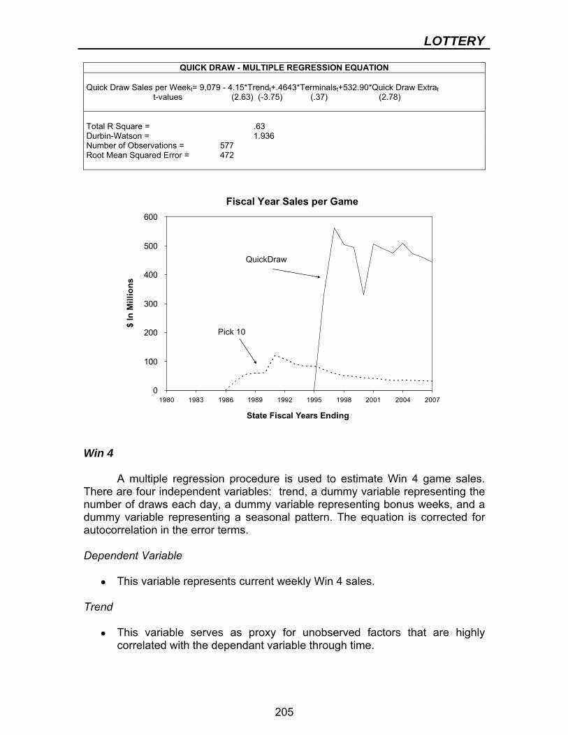
LOTTERY
205
QUICK DRAW - MULTIPLE REGRESSION EQUATION Quick Draw Sales per Weekt= 9,079 - 4.15*Trendt+.4643*Terminalst+532.90*Quick Draw Extrat t-values (2.63) (-3.75) (.37) (2.78) Total R Square = .63 Durbin-Watson = 1.936 Number of Observations = 577 Root Mean Squared Error = 472
Fiscal Year Sales per Game
0
100
200
300
400
500
600
1980 1983 1986 1989 1992 1995 1998 2001 2004 2007
State Fiscal Years Ending
$ In
Mill
ions
QuickDraw
Pick 10
Win 4 A multiple regression procedure is used to estimate Win 4 game sales. There are four independent variables: trend, a dummy variable representing the number of draws each day, a dummy variable representing bonus weeks, and a dummy variable representing a seasonal pattern. The equation is corrected for autocorrelation in the error terms. Dependent Variable
● This variable represents current weekly Win 4 sales. Trend
● This variable serves as proxy for unobserved factors that are highly correlated with the dependant variable through time.

LOTTERY
206
Draws Per Day
● A dummy variable reflecting the number of Win 4 draws per day. On December 2, 2001, the Lottery Division launched a second daily draw, a noon draw for the Numbers and the Win 4 games. The dummy variable is zero prior to and including November 24, 2001, and one thereafter.
Bonus Week
● This is a dummy variable reflecting scheduled promotional bonus weeks for this game. The dummy variable is zero in every week before and after scheduled bonus weeks, and is one during the bonus weeks.
Seasonal Dummy
● Equal to one in the months of February through May and zero during the rest of the year, reflecting historically higher sales during this period of the year.
WIN 4 - MULTIPLE REGRESSION EQUATION
Win 4 Sales per Weekt = 5,703 + 5.94*Trendt+918.8*Draws Per Dayt + 224.87*Bonus Weekt +238.87*Seasonal Dummyt t-values (31.96) (20.15) (7.15) (3.75) (3.98) Total R Square = .98 Durbin-Watson = 2.0374 Number of Observations = 852 Root Mean Squared Error = 313
Daily Numbers Game The Daily Numbers sales are estimated by employing a multiple regression equation. There are four independent variables: the number of draws per day, a trend and a dummy variable representing bonus weeks, and a dummy variable representing a seasonal pattern. The equation is corrected for autocorrelation in the error terms. Dependent Variable
● This variable represents current weekly Daily Numbers sales. Trend
● This variable serves as proxy for unobserved factors that are highly correlated with the dependant variable through time.

LOTTERY
207
Draws Per Day
● This dummy variable reflects the number of Daily Number draws per day. On December 2, 2001, the Lottery Division launched a second daily draw, a noon draw, for the Numbers and the Win 4 games. The dummy variable is zero prior to and including November 24, 2001, and one thereafter.
Bonus Week
● This dummy variable reflects scheduled promotional bonus weeks for this game. The dummy variable is zero in every week before and after scheduled bonus weeks, and is one during the bonus weeks.
Seasonal Dummy
● Equal to one in the months of February through May and zero during the rest of the year, reflecting historically higher sales during this period of the year.
DAILY NUMBERS - MULTIPLE REGRESSION EQUATION
Daily Numbers Sales per Weekt = 11,736 + 2.96*Trendt + 732.29*Draws Per Dayt + 521.13*Bonus Weekt+312.16*Seasonal Dummyt t-values (29.27) (5.34) (3.79) (4.97) (3.09) Total R Square = .85 Durbin-Watson = 1.91 Number of Observations = 601 Root Mean Squared Error = 463
Take 5 Take 5 sales are estimated using a multiple regression equation. There are three independent variables: a variable representing the change in prize payout percent from 40 percent to 50 percent, a variable reflecting the number of draws offered each week, and a dummy variable representing competition from the Mega Millions game. Essentially, these three special events explain most of the change in Take 5 sales. The equation is corrected for autocorrelation in the error terms. Dependent Variable
● This variable represents current weekly Take 5 sales. Trend
● This variable serves as proxy for unobserved factors that are highly correlated with the dependant variable through time.
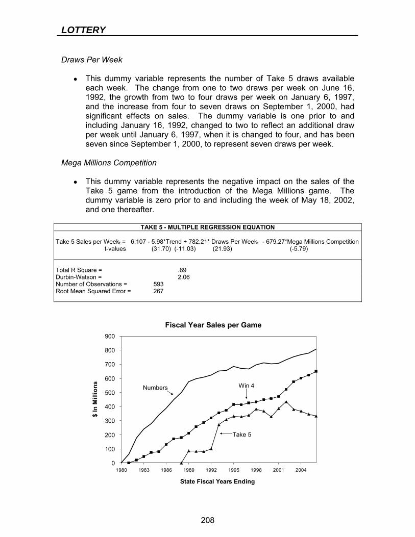
LOTTERY
208
Draws Per Week
● This dummy variable represents the number of Take 5 draws available each week. The change from one to two draws per week on June 16, 1992, the growth from two to four draws per week on January 6, 1997, and the increase from four to seven draws on September 1, 2000, had significant effects on sales. The dummy variable is one prior to and including January 16, 1992, changed to two to reflect an additional draw per week until January 6, 1997, when it is changed to four, and has been seven since September 1, 2000, to represent seven draws per week.
Mega Millions Competition
● This dummy variable represents the negative impact on the sales of the Take 5 game from the introduction of the Mega Millions game. The dummy variable is zero prior to and including the week of May 18, 2002, and one thereafter.
TAKE 5 - MULTIPLE REGRESSION EQUATION
Take 5 Sales per Weekt = 6,107 - 5.98*Trend + 782.21* Draws Per Weekt - 679.27*Mega Millions Competition t-values (31.70) (-11.03) (21.93) (-5.79) Total R Square = .89 Durbin-Watson = 2.06 Number of Observations = 593 Root Mean Squared Error = 267
Fiscal Year Sales per Game
0
100
200
300
400
500
600
700
800
900
1980 1983 1986 1989 1992 1995 1998 2001 2004
State Fiscal Years Ending
$ In
Mill
ions Numbers Win 4
Take 5
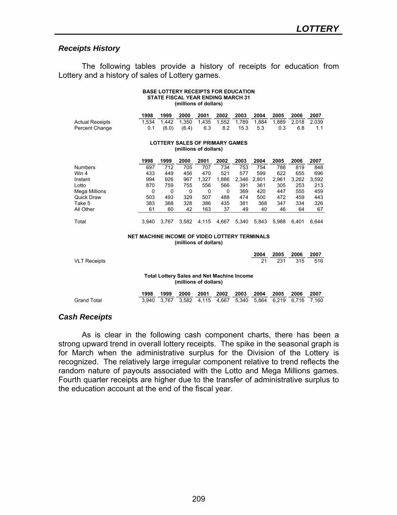
LOTTERY
209
Receipts History The following tables provide a history of receipts for education from Lottery and a history of sales of Lottery games.
BASE LOTTERY RECEIPTS FOR EDUCATION STATE FISCAL YEAR ENDING MARCH 31
(millions of dollars)
1998 1999 2000 2001 2002 2003 2004 2005 2006 2007 Actual Receipts 1,534 1,442 1,350 1,435 1,552 1,789 1,884 1,889 2,018 2,039Percent Change 0.1 (6.0) (6.4) 6.3 8.2 15.3 5.3 0.3 6.8 1.1
LOTTERY SALES OF PRIMARY GAMES
(millions of dollars)
1998 1999 2000 2001 2002 2003 2004 2005 2006 2007 Numbers 697 712 705 707 734 753 754 788 819 848Win 4 433 449 456 470 521 577 599 622 655 696Instant 994 926 967 1,327 1,886 2,346 2,801 2,961 3,262 3,592Lotto 870 759 755 556 566 391 361 305 253 213Mega Millions 0 0 0 0 0 369 420 447 555 459Quick Draw 503 493 329 507 488 474 500 472 459 443Take 5 383 368 328 386 435 381 368 347 334 326All Other 61 60 42 163 37 49 40 46 64 67 Total 3,940 3,767 3,582 4,115 4,667 5,340 5,843 5,988 6,401 6,644
NET MACHINE INCOME OF VIDEO LOTTERY TERMINALS
(millions of dollars)
2004 2005 2006 2007 VLT Receipts 21 231 315 516
Total Lottery Sales and Net Machine Income
(millions of dollars)
1998 1999 2000 2001 2002 2003 2004 2005 2006 2007 Grand Total 3,940 3,767 3,582 4,115 4,667 5,340 5,864 6,219 6,716 7,160
Cash Receipts As is clear in the following cash component charts, there has been a strong upward trend in overall lottery receipts. The spike in the seasonal graph is for March when the administrative surplus for the Division of the Lottery is recognized. The relatively large irregular component relative to trend reflects the random nature of payouts associated with the Lotto and Mega Millions games. Fourth quarter receipts are higher due to the transfer of administrative surplus to the education account at the end of the fiscal year.
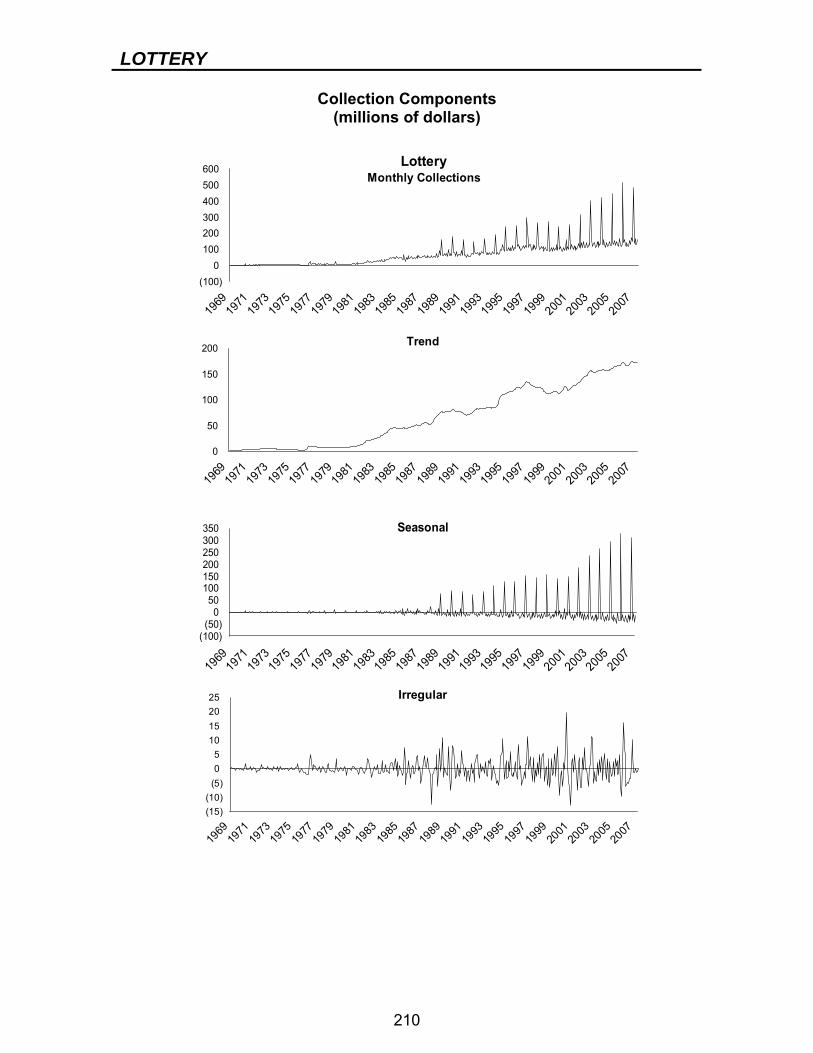
LOTTERY
210
Collection Components (millions of dollars)
(100)0
100200300400500600
1969
1971
1973
1975
1977
1979
1981
1983
1985
1987
1989
1991
1993
1995
1997
1999
2001
2003
2005
2007
LotteryMonthly Collections
0
50
100
150
200
1969
1971
1973
1975
1977
1979
1981
1983
1985
1987
1989
1991
1993
1995
1997
1999
2001
2003
2005
2007
Trend
(100)(50)
050
100150200250300350
1969
1971
1973
1975
1977
1979
1981
1983
1985
1987
1989
1991
1993
1995
1997
1999
2001
2003
2005
2007
Seasonal
(15)(10)
(5)05
10152025
1969
1971
1973
1975
1977
1979
1981
1983
1985
1987
1989
1991
1993
1995
1997
1999
2001
2003
2005
2007
Irregular
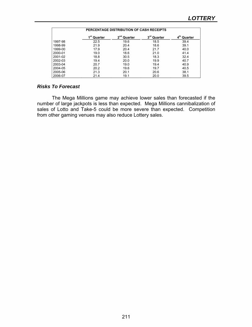
LOTTERY
211
PERCENTAGE DISTRIBUTION OF CASH RECEIPTS
1st Quarter 2nd Quarter 3rd Quarter 4th Quarter 1997-98 22.5 19.6 18.5 39.4 1998-99 21.9 20.4 18.6 39.1 1999-00 17.9 20.4 21.7 40.0 2000-01 19.0 18.6 21.0 41.4 2001-02 18.8 30.5 18.3 32.4 2002-03 19.4 20.0 19.9 40.7 2003-04 20.7 19.0 19.4 40.9 2004-05 20.2 19.6 19.7 40.5 2005-06 21.3 20.1 20.6 38.1 2006-07 21.4 19.1 20.0 39.5
Risks To Forecast The Mega Millions game may achieve lower sales than forecasted if the number of large jackpots is less than expected. Mega Millions cannibalization of sales of Lotto and Take-5 could be more severe than expected. Competition from other gaming venues may also reduce Lottery sales.
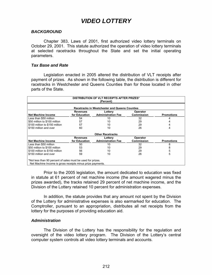
212
VIDEO LOTTERY BACKGROUND Chapter 383, Laws of 2001, first authorized video lottery terminals on October 29, 2001. This statute authorized the operation of video lottery terminals at selected racetracks throughout the State and set the initial operating parameters. Tax Base and Rate Legislation enacted in 2005 altered the distribution of VLT receipts after payment of prizes. As shown in the following table, the distribution is different for racetracks in Westchester and Queens Counties than for those located in other parts of the State.
DISTRIBUTION OF VLT RECEIPTS AFTER PRIZES* (Percent)
Racetracks in Westchester and Queens Counties
Net Machine Income
Revenues for Education
Lottery Administration Fee
Operator Commission
Promotions
Less than $50 million 54 10 32 4 $50 million to $100 million 57 10 29 4 $100 million to $150 million 57 10 29 4 $150 million and over 60 10 26 4
Other Racetracks Net Machine Income
Revenues for Education
Lottery Administration Fee
Operator Commission
Promotions
Less than $50 million 50 10 32 8 $50 million to $100 million 53 10 29 8 $100 million to $150 million 56 10 29 5 $150 million and over 59 10 26 5 *Not less than 90 percent of sales must be used for prizes. Net Machine Income is gross receipts minus prize payments.
Prior to the 2005 legislation, the amount dedicated to education was fixed in statute at 61 percent of net machine income (the amount wagered minus the prizes awarded), the tracks retained 29 percent of net machine income, and the Division of the Lottery retained 10 percent for administration expenses. In addition, the statute provides that any amount not spent by the Division of the Lottery for administrative expenses is also earmarked for education. The Comptroller, pursuant to an appropriation, distributes all net receipts from the lottery for the purposes of providing education aid. Administration The Division of the Lottery has the responsibility for the regulation and oversight of the video lottery program. The Division of the Lottery’s central computer system controls all video lottery terminals and accounts.
VIDEO LOTTERY
213
DATA SOURCES The data available on VLT operations are collected and reported by the Division of the Lottery. STATUTORY CHANGES Legislation was enacted, on October 29, 2001, to allow the Division of the Lottery to license the operation of VLTs at selected New York State racetracks. Additional legislation enacted on May 2, 2003, made the following major adjustments to the VLT program:
● Of the revenue remaining after payment of prizes, the Division of the Lottery retains 10 percent commission, the racetracks receive 29 percent, and 61 percent is dedicated to education.
● Of the 29 percent commission paid to the tracks, the amount allocated to horse racing purses in years one through three is 25.9 percent; in years four and five, 26.7 percent; and in subsequent years, 34.5 percent.
● Of the 29 percent commission paid to the tracks, the harness and thoroughbred Breeders’ funds receive 4.3 percent in the first through fifth years and 5.2 percent in all the following years.
● The racetracks are allowed to enter into agreements with the horse owners for no longer than five years, to allow the tracks to retain a portion of the revenue dedicated to purses for the operation of the facilities. The program expires after ten years.
Legislation enacted on April 12, 2005 revised the distribution of VLT receipts, providing:
● A graduated vendor’s fee that allows participating tracks to receive 32 percent of the first $50 million of revenue after prizes, 29 percent of the next $100 million, and 26 percent of net revenue over $150 million.
● A marketing allowance of 8 percent of the first $100 million of net revenue and 5 percent thereafter. The marketing allowance is limited to 4 percent of net revenue for tracks located in Westchester or Queens counties.
● An extension of the program’s expiration until December 31, 2017. ● The statutory allocations to purses and breeders funds were eliminated.
FORECAST METHODOLOGY The forecasting methodology used by the Division of the Budget relies on a complex simulation model to forecast potential revenues from all facilities that either are in existence or are expected to begin operation during the forecast period. The methodology is modified after a specific facility has operated long enough to produce a sufficient number of observations. At this point, actual operating experience is used to recalibrate the model.
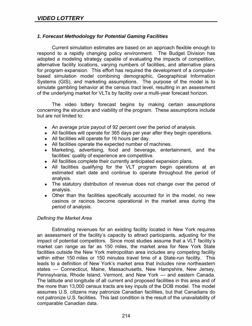
VIDEO LOTTERY
214
1. Forecast Methodology for Potential Gaming Facilities Current simulation estimates are based on an approach flexible enough to respond to a rapidly changing policy environment. The Budget Division has adopted a modeling strategy capable of evaluating the impacts of competition, alternative facility locations, varying numbers of facilities, and alternative plans for program expansion. This effort has required the development of a computer-based simulation model combining demographic, Geographical Information Systems (GIS), and marketing assumptions. The purpose of the model is to simulate gambling behavior at the census tract level, resulting in an assessment of the underlying market for VLTs by facility over a multi-year forecast horizon. The video lottery forecast begins by making certain assumptions concerning the structure and viability of the program. These assumptions include but are not limited to:
● An average prize payout of 92 percent over the period of analysis. ● All facilities will operate for 365 days per year after they begin operations. ● All facilities will operate for 16 hours per day. ● All facilities operate the expected number of machines. ● Marketing, advertising, food and beverage, entertainment, and the
facilities’ quality of experience are competitive. ● All facilities complete their currently anticipated expansion plans. ● All facilities qualifying for the VLT program begin operations at an
estimated start date and continue to operate throughout the period of analysis.
● The statutory distribution of revenue does not change over the period of analysis.
● Other than the facilities specifically accounted for in the model, no new casinos or racinos become operational in the market area during the period of analysis.
Defining the Market Area Estimating revenues for an existing facility located in New York requires an assessment of the facility’s capacity to attract participants, adjusting for the impact of potential competitors. Since most studies assume that a VLT facility’s market can range as far as 150 miles, the market area for New York State facilities outside the New York metropolitan area includes any competing facility within either 150 miles or 150 minutes travel time of a State-run facility. This leads to a definition of New York’s market area that includes nine northeastern states — Connecticut, Maine, Massachusetts, New Hampshire, New Jersey, Pennsylvania, Rhode Island, Vermont, and New York — and eastern Canada. The latitude and longitude of all current and proposed facilities in this area and of the more than 13,000 census tracts are key inputs of the DOB model. The model assumes U.S. citizens may patronize Canadian facilities, but that Canadians do not patronize U.S. facilities. This last condition is the result of the unavailability of comparable Canadian data.

VIDEO LOTTERY
215
An evaluation of the market potential for video lottery terminals and slot machines in New York requires an assessment of four critical market characteristics:
1. The number of potential participants living in the New York market area. 2. The frequency with which participants visit a casino or VLT facility. 3. The amount spent per visit to a facility. 4. The selection of several potential facilities that a participant will visit.
Number of Participants Estimating the potential number of participants begins with a national demographic profile of people who typically patronize casinos. The primary source of this data is gambling industry trade publications. These data indicate the percentage of potential gamblers for four demographic characteristics: age, income, gender, and education. The same data also give an aggregate participation rate for each state. To account for differences among the states’ participation rates, national rates for each demographic variable are adjusted to reflect the state-specific participation rate. Using the adjusted data, the number of participants are estimated by applying state-specific participation rates to each of the four demographic characteristics for each census tract in the nine-state study area. This provides an indication by census tract of how many people in the nine-state market area are likely to visit a casino or VLT facility. To arrive at a multi-year monthly forecast, each of the four demographic characteristics and participation rates are projected by month and census track to March 2012. The appropriate monthly participation rate is applied to each of the four demographic categories in each census tract to arrive at four monthly estimates of the number of potential participants in each census tract. An unweighted average of the four estimates is used to arrive at a final estimate. The estimated participation rates of some fully mature states, such as New Jersey and Connecticut, are increased modestly over the projection period. This provides an estimate of the number of gamblers in each census tract by month through March 2012.
UNITED STATES POPULATIONEDUCATION (Age 25+)
25%
18%
10%
47% No CollegeSome CollegeBachelor's DegreePost Bachelor's
Source: The AGA Survey of USA Casino Entertainment 2006
UNITED STATES CASINOCUSTOMERS EDUCATION (Age 25+)
29%
8%
18%
45% No CollegeSome CollegeBachelor's DegreePost Bachelor's
Source: The AGA Survey of USA Casino Entertainment 2006
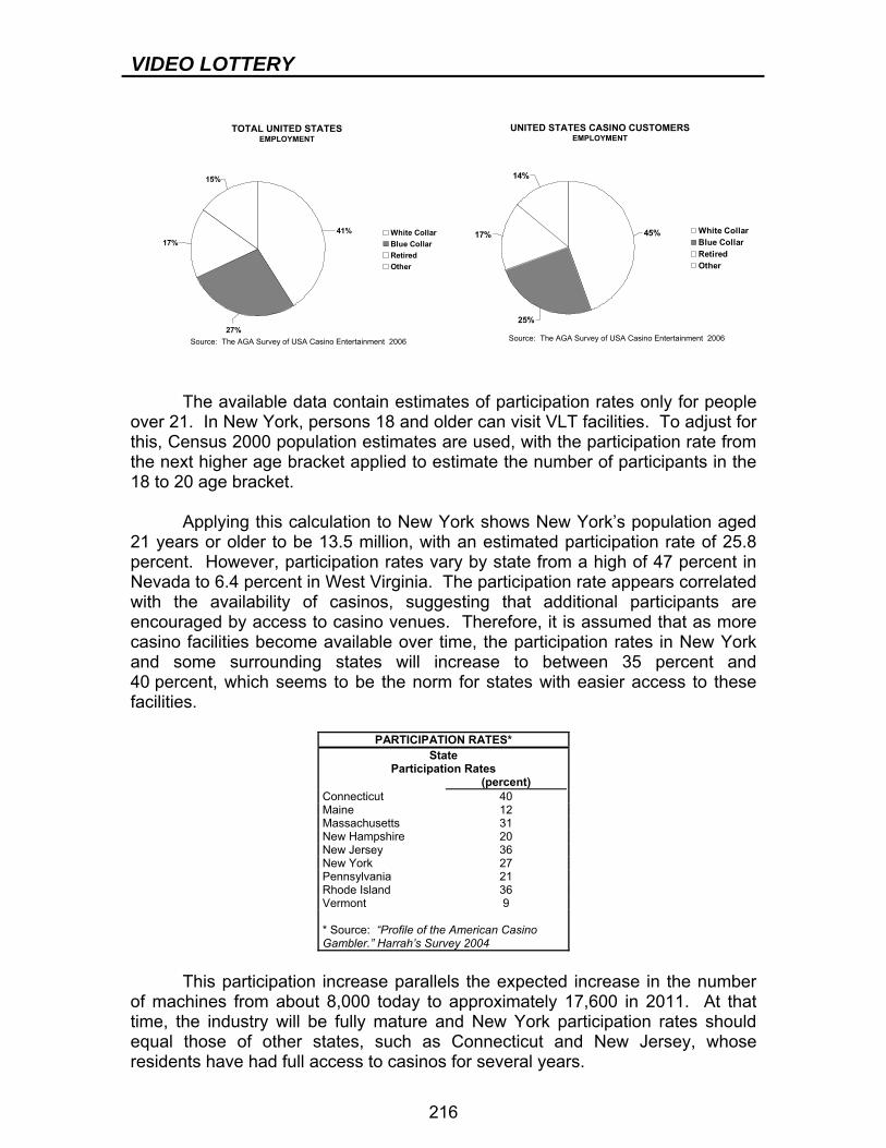
VIDEO LOTTERY
216
The available data contain estimates of participation rates only for people over 21. In New York, persons 18 and older can visit VLT facilities. To adjust for this, Census 2000 population estimates are used, with the participation rate from the next higher age bracket applied to estimate the number of participants in the 18 to 20 age bracket. Applying this calculation to New York shows New York’s population aged 21 years or older to be 13.5 million, with an estimated participation rate of 25.8 percent. However, participation rates vary by state from a high of 47 percent in Nevada to 6.4 percent in West Virginia. The participation rate appears correlated with the availability of casinos, suggesting that additional participants are encouraged by access to casino venues. Therefore, it is assumed that as more casino facilities become available over time, the participation rates in New York and some surrounding states will increase to between 35 percent and 40 percent, which seems to be the norm for states with easier access to these facilities.
PARTICIPATION RATES* State
Participation Rates (percent) Connecticut 40 Maine 12 Massachusetts 31 New Hampshire 20 New Jersey 36 New York 27 Pennsylvania 21 Rhode Island 36 Vermont 9 * Source: “Profile of the American Casino Gambler.” Harrah’s Survey 2004
This participation increase parallels the expected increase in the number of machines from about 8,000 today to approximately 17,600 in 2011. At that time, the industry will be fully mature and New York participation rates should equal those of other states, such as Connecticut and New Jersey, whose residents have had full access to casinos for several years.
TOTAL UNITED STATESEMPLOYMENT
27%
17%
15%
41% White CollarBlue CollarRetiredOther
Source: The AGA Survey of USA Casino Entertainment 2006
UNITED STATES CASINO CUSTOMERSEMPLOYMENT
25%
17%
14%
45% White CollarBlue CollarRetiredOther
Source: The AGA Survey of USA Casino Entertainment 2006

VIDEO LOTTERY
217
The Harrah’s Survey 2006 Profile of the American Casino Gambler cites New York City as already having a 33 percent participation rate and further notes the New York Metro region as the number 1 “feeder” market for casino trips. Number of Visits To estimate the frequency of visits, two approaches are combined. First, several published studies indicate that the closer an individual lives to a casino, the more frequent the visits. One study by KPMG postulated that a typical person within the primary market area of a casino (less than 50 miles) would visit on average ten times per year. A person within the secondary market area (50 miles to 100 miles) would visit six times per year on average and in the tertiary area (100 miles to 150 miles), three times per year. The American Gaming Association survey found that nationally the average casino player visits a casino 6.1 times per year. In the Northeast region, the average casino player visits 8.5 times per year. Again, the Profile gives the average number of visits by state; it appears that the number of visits increases in states with higher participation rates. The analysis has been calibrated using both studies, and the results from both approaches are relatively close. The number of visits is estimated monthly by census tract as population and participation rates rise over time, and are combined to produce a final forecast. Amount Gambled To determine the amount of income spent per visit, two studies were used. Oregon completed a study that indicated that the average person would gamble approximately 1.16 percent of annual income on all forms of gaming. On the other hand, KPMG, in its study of gambling in Michigan, postulated that people in the primary market area would be willing to lose $40 each time they visited a casino, in the secondary market area $50 each time, and in the tertiary market area $65 each time. To derive the amount of gambling dollars using the KPMG methodology, the loss per visit was increased or decreased by indexing these amounts by the ratio of the per capita income of each census tract to the per capita income in Michigan. To grow the amount gambled in each census tract, personal income and population were increased by the growth rate between the 1990 and 2000 census. This allowed for growth in the amount gambled in the primary, secondary, and tertiary market areas by month through 2011. This also allowed calculation of the total amount of gambling dollars in each census tract by multiplying personal income by the Oregon average percentage of income gambled. Somewhat surprisingly, these two methodologies produced similar results. The amount gambled in each census tract is forecast monthly to 2011 as a function of the growth in population, income, and participation rates. Defining the Market Area for Each Facility The VLT analysis next concentrates on allocating the aggregate number of visits and gaming dollars in New York’s market area to the potential venues. There are several existing facilities in New York, the surrounding states and Canada, and over the next five years, new facilities may open. Each facility will
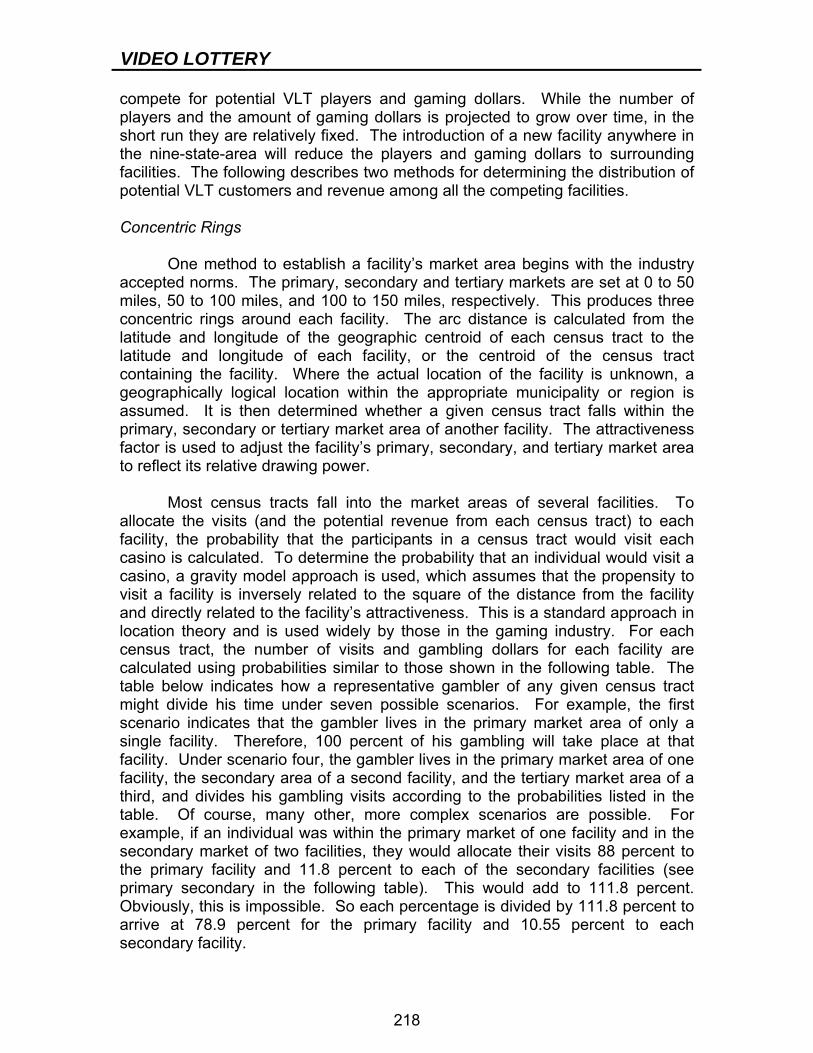
VIDEO LOTTERY
218
compete for potential VLT players and gaming dollars. While the number of players and the amount of gaming dollars is projected to grow over time, in the short run they are relatively fixed. The introduction of a new facility anywhere in the nine-state-area will reduce the players and gaming dollars to surrounding facilities. The following describes two methods for determining the distribution of potential VLT customers and revenue among all the competing facilities. Concentric Rings One method to establish a facility’s market area begins with the industry accepted norms. The primary, secondary and tertiary markets are set at 0 to 50 miles, 50 to 100 miles, and 100 to 150 miles, respectively. This produces three concentric rings around each facility. The arc distance is calculated from the latitude and longitude of the geographic centroid of each census tract to the latitude and longitude of each facility, or the centroid of the census tract containing the facility. Where the actual location of the facility is unknown, a geographically logical location within the appropriate municipality or region is assumed. It is then determined whether a given census tract falls within the primary, secondary or tertiary market area of another facility. The attractiveness factor is used to adjust the facility’s primary, secondary, and tertiary market area to reflect its relative drawing power. Most census tracts fall into the market areas of several facilities. To allocate the visits (and the potential revenue from each census tract) to each facility, the probability that the participants in a census tract would visit each casino is calculated. To determine the probability that an individual would visit a casino, a gravity model approach is used, which assumes that the propensity to visit a facility is inversely related to the square of the distance from the facility and directly related to the facility’s attractiveness. This is a standard approach in location theory and is used widely by those in the gaming industry. For each census tract, the number of visits and gambling dollars for each facility are calculated using probabilities similar to those shown in the following table. The table below indicates how a representative gambler of any given census tract might divide his time under seven possible scenarios. For example, the first scenario indicates that the gambler lives in the primary market area of only a single facility. Therefore, 100 percent of his gambling will take place at that facility. Under scenario four, the gambler lives in the primary market area of one facility, the secondary area of a second facility, and the tertiary market area of a third, and divides his gambling visits according to the probabilities listed in the table. Of course, many other, more complex scenarios are possible. For example, if an individual was within the primary market of one facility and in the secondary market of two facilities, they would allocate their visits 88 percent to the primary facility and 11.8 percent to each of the secondary facilities (see primary secondary in the following table). This would add to 111.8 percent. Obviously, this is impossible. So each percentage is divided by 111.8 percent to arrive at 78.9 percent for the primary facility and 10.55 percent to each secondary facility.
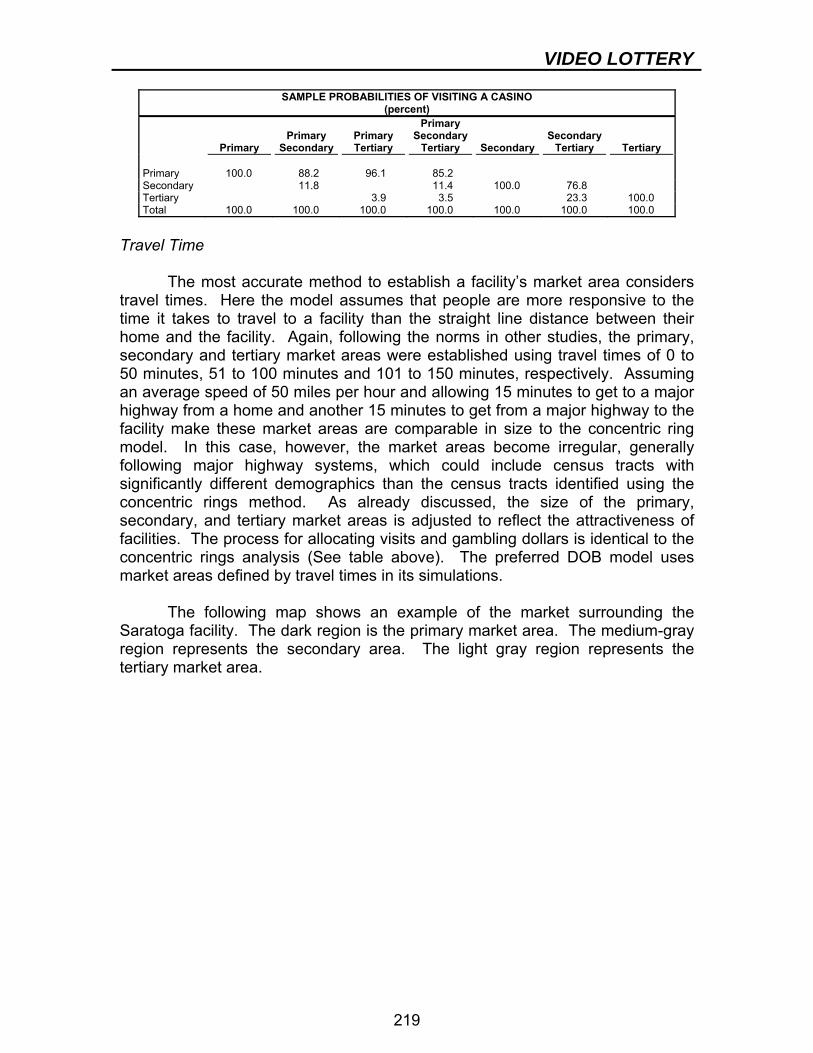
VIDEO LOTTERY
219
SAMPLE PROBABILITIES OF VISITING A CASINO (percent)
Primary
Primary
Secondary
Primary Tertiary
Primary Secondary
Tertiary
Secondary
Secondary
Tertiary
Tertiary Primary 100.0 88.2 96.1 85.2 Secondary 11.8 11.4 100.0 76.8 Tertiary 3.9 3.5 23.3 100.0 Total 100.0 100.0 100.0 100.0 100.0 100.0 100.0
Travel Time The most accurate method to establish a facility’s market area considers travel times. Here the model assumes that people are more responsive to the time it takes to travel to a facility than the straight line distance between their home and the facility. Again, following the norms in other studies, the primary, secondary and tertiary market areas were established using travel times of 0 to 50 minutes, 51 to 100 minutes and 101 to 150 minutes, respectively. Assuming an average speed of 50 miles per hour and allowing 15 minutes to get to a major highway from a home and another 15 minutes to get from a major highway to the facility make these market areas are comparable in size to the concentric ring model. In this case, however, the market areas become irregular, generally following major highway systems, which could include census tracts with significantly different demographics than the census tracts identified using the concentric rings method. As already discussed, the size of the primary, secondary, and tertiary market areas is adjusted to reflect the attractiveness of facilities. The process for allocating visits and gambling dollars is identical to the concentric rings analysis (See table above). The preferred DOB model uses market areas defined by travel times in its simulations. The following map shows an example of the market surrounding the Saratoga facility. The dark region is the primary market area. The medium-gray region represents the secondary area. The light gray region represents the tertiary market area.
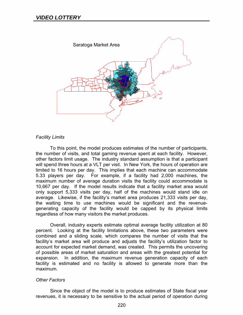
VIDEO LOTTERY
220
Saratoga Market Area
Facility Limits To this point, the model produces estimates of the number of participants, the number of visits, and total gaming revenue spent at each facility. However, other factors limit usage. The industry standard assumption is that a participant will spend three hours at a VLT per visit. In New York, the hours of operation are limited to 16 hours per day. This implies that each machine can accommodate 5.33 players per day. For example, if a facility had 2,000 machines, the maximum number of average duration visits the facility could accommodate is 10,667 per day. If the model results indicate that a facility market area would only support 5,333 visits per day, half of the machines would stand idle on average. Likewise, if the facility’s market area produces 21,333 visits per day, the waiting time to use machines would be significant and the revenue-generating capacity of the facility would be capped by its physical limits regardless of how many visitors the market produces. Overall, industry experts estimate optimal average facility utilization at 80 percent. Looking at the facility limitations above, these two parameters were combined and a sliding scale, which compares the number of visits that the facility’s market area will produce and adjusts the facility’s utilization factor to account for expected market demand, was created. This permits the uncovering of possible areas of market saturation and areas with the greatest potential for expansion. In addition, the maximum revenue generation capacity of each facility is estimated and no facility is allowed to generate more than the maximum. Other Factors Since the object of the model is to produce estimates of State fiscal year revenues, it is necessary to be sensitive to the actual period of operation during
VIDEO LOTTERY
221
each fiscal year and to the competitive effects of other facilities. For the tracks, the most recent information available from the Lottery Division is used to specify expected start dates and the initial number of machines, expansion of existing facilities, and changes in machine counts. The model also has the ability to add new facilities anywhere in the Northeast and to adjust to any expansion plans anticipated by the tracks or other facilities. To attempt to reflect the competitive impact of the recently authorized Native American casinos on the State’s VLT facilities and visa versa, start dates and the number of terminals at each anticipated facility are assumed. At this time, however, the start dates, the number of machines and other parameters for the new Native American casinos are highly speculative, but to avoid over-estimating revenues from VLT facilities this factor must be considered. Simulation Model Aggregate Results Aggregate results for this model depend upon the combination of gaming facilities open during a particular fiscal year and other factors such as start dates, quantity of VLTs or slots offered, additional amenities, and several other situational gaming factors. Given an almost infinite number of different scenarios, estimated results of the quantity of gamblers, total net machine income, and total visits can be illustrated in a low to high range. The higher numbers in the range assume a more mature gaming market in year 2011, when New York State’s gaming participation has attained levels comparable to adjacent states. 2. Forecast Methodology Subsequent to the Opening of a VLT or Casino Facility The factors effecting receipts for existing facilities are not unlike that for potential facilities. In addition to the assumptions concerning the market area, number of participants, number of visits and amount gambled, data on marketing and promotions can be included in the analysis. After a facility has been opened long enough to compile a historic data series, the simulation model is calibrated to approximate the attractiveness factor. Historical data on each facility’s net machine income trends can now be incorporated into the forecast. Consideration is also given to expansion and improvements to facilities as well as competition from other gaming venues. Currently, there are eight VLT facilities in operation: Saratoga Gaming and Raceway, Finger Lakes Gaming and Racetrack, Fairgrounds Gaming and Raceway at Buffalo, Mighty M Gaming at Monticello, Yonkers Raceway, Tioga Downs, Batavia Downs, and Vernon Downs. It is currently anticipated that and Aqueduct will open in 2009.
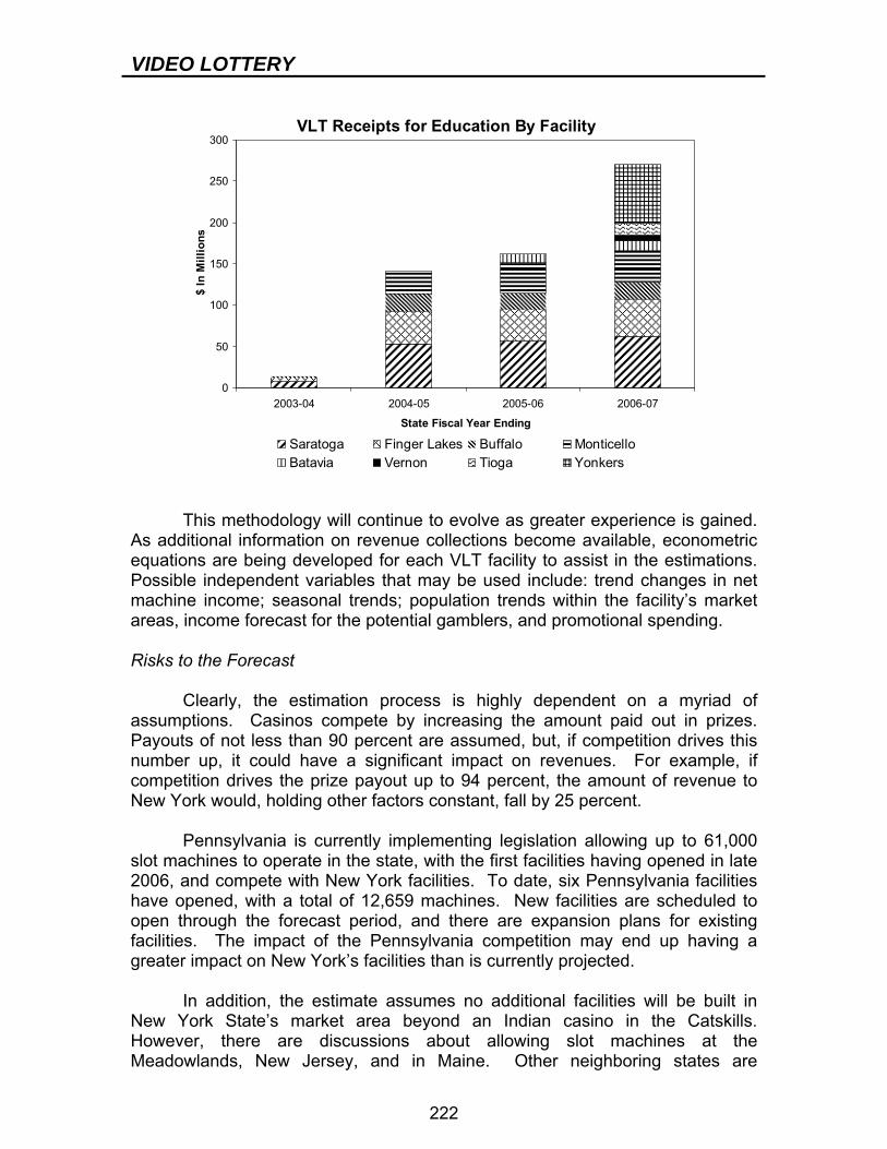
VIDEO LOTTERY
222
VLT Receipts for Education By Facility
0
50
100
150
200
250
300
2003-04 2004-05 2005-06 2006-07
State Fiscal Year Ending
$ In
Mill
ions
Saratoga Finger Lakes Buffalo MonticelloBatavia Vernon Tioga Yonkers
This methodology will continue to evolve as greater experience is gained. As additional information on revenue collections become available, econometric equations are being developed for each VLT facility to assist in the estimations. Possible independent variables that may be used include: trend changes in net machine income; seasonal trends; population trends within the facility’s market areas, income forecast for the potential gamblers, and promotional spending. Risks to the Forecast Clearly, the estimation process is highly dependent on a myriad of assumptions. Casinos compete by increasing the amount paid out in prizes. Payouts of not less than 90 percent are assumed, but, if competition drives this number up, it could have a significant impact on revenues. For example, if competition drives the prize payout up to 94 percent, the amount of revenue to New York would, holding other factors constant, fall by 25 percent. Pennsylvania is currently implementing legislation allowing up to 61,000 slot machines to operate in the state, with the first facilities having opened in late 2006, and compete with New York facilities. To date, six Pennsylvania facilities have opened, with a total of 12,659 machines. New facilities are scheduled to open through the forecast period, and there are expansion plans for existing facilities. The impact of the Pennsylvania competition may end up having a greater impact on New York’s facilities than is currently projected. In addition, the estimate assumes no additional facilities will be built in New York State’s market area beyond an Indian casino in the Catskills. However, there are discussions about allowing slot machines at the Meadowlands, New Jersey, and in Maine. Other neighboring states are

VIDEO LOTTERY
223
considering authorizing racinos, and there are continual expansions at Foxwoods, Mohegan Sun and Turning Stone. On the other hand, the market for video lottery gaming could be greater than anticipated, especially in the New York City metropolitan area. If this proves to be correct, the estimates of net machine income could be understated and the estimates of losses due to competition might be too high.


Part III - Spending Methodologies

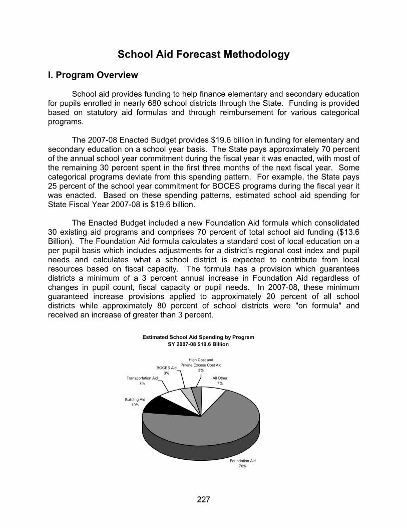
227
School Aid Forecast Methodology I. Program Overview School aid provides funding to help finance elementary and secondary education for pupils enrolled in nearly 680 school districts through the State. Funding is provided based on statutory aid formulas and through reimbursement for various categorical programs. The 2007-08 Enacted Budget provides $19.6 billion in funding for elementary and secondary education on a school year basis. The State pays approximately 70 percent of the annual school year commitment during the fiscal year it was enacted, with most of the remaining 30 percent spent in the first three months of the next fiscal year. Some categorical programs deviate from this spending pattern. For example, the State pays 25 percent of the school year commitment for BOCES programs during the fiscal year it was enacted. Based on these spending patterns, estimated school aid spending for State Fiscal Year 2007-08 is $19.6 billion. The Enacted Budget included a new Foundation Aid formula which consolidated 30 existing aid programs and comprises 70 percent of total school aid funding ($13.6 Billion). The Foundation Aid formula calculates a standard cost of local education on a per pupil basis which includes adjustments for a district’s regional cost index and pupil needs and calculates what a school district is expected to contribute from local resources based on fiscal capacity. The formula has a provision which guarantees districts a minimum of a 3 percent annual increase in Foundation Aid regardless of changes in pupil count, fiscal capacity or pupil needs. In 2007-08, these minimum guaranteed increase provisions applied to approximately 20 percent of all school districts while approximately 80 percent of school districts were "on formula" and received an increase of greater than 3 percent.
Estimated School Aid Spending by ProgramSY 2007-08 $19.6 Billion
All Other7%
Foundation Aid70%
Building Aid10%
BOCES Aid3%
High Cost and Private Excess Cost Aid
3%
Transportation Aid7%

SCHOOL AID
228
II. Key Forecasting Data and Assumptions Education Law requires the State Education Department (SED) to release school district specific data three times a year on February 15, May 15 and November 15 for the purposes of calculating school aid. Traditionally, the November 15 database forms the basis for Executive Budget forecasts. The February and May database updates are used to revise forecasts of school aid to individual districts. Data factors from the School Aid Databases that drive school aid include the following:
District wealth and fiscal capacity based on income per pupil and actual valuation of taxable property per pupil. Pupil needs such as measures of student poverty, student special education needs counts of students with limited English proficiency and geographic scarcity. Approved Spending for instructional materials, transportation, school construction and other needs. District expenditures for such purposes are reviewed and approved by SED. Pupil counts such as public school attendance, counts of students eligible for free and reduced price lunch programs, pupils with limited ability in English and the like. In addition to these school district specific measures, the recently enacted
Foundation Aid formula provides for an adjustment of the standard cost of lower education for changes in the consumer price index (CPI). DOB’s U.S. Macroeconomic model forecasts CPI and this forecast is incorporated into school aid projections.
Below are examples of three of the largest school aid formulas/programs,
providing details of the data elements and detail regarding the formula models and assumptions. For the 2007-08 school year, the aid calculations detailed below (Foundation Aid, Transportation Aid and Building Aid) amount to $16.8 billion, or 85 percent, of total State school aid funding. For the remaining expense-based categorical programs, the DOB performs multi-year growth trend analyses to develop a forecast. Foundation Aid ($13,640 million) In the 2007-08 School Year, Foundation Aid allocates $13.6 billion in State funds, a $1.1 billion or 8.8 percent increase from the 2006-07 School Year. Over the next four years, Foundation Aid is expected to grow by $5.5 billion to a total of $18.1 billion in 2010-11.
SCHOOL AID
229
The per pupil Foundation Aid calculation is based on the standard cost of education determined by the SED. This is the cost of educating an "average" student in schools that are performing well as measured by SED Statewide test results. The standard cost of education per pupil ($5,258 for 2007-08) is estimated to be $5,662 for the 2010-11 School Year. This standard cost of education is adjusted on an annual basis to increases in the CPI. Additional adjustments are made to take into account pupil needs and regional cost variations. A Pupil Needs Index, which ranges from 1.0 to 2.0, adjusts the standard cost of education amount for students in poverty—those eligible for free and reduced price lunch as measured by census poverty data—limited English proficient pupils, and students educated in the State's rural districts. Regional cost adjustments are based on an SED analysis of median salaries for 59 professional occupations other than teaching. Indices are established for nine labor market regions and range from 1.000 for counties in the North Country and Mohawk Valley to 1.425 for Long Island and New York City. For the 2010-11 School Year, the Foundation Aid per pupil amount will be the greater of $5,662 times the pupil needs index and regional cost index minus (a) an expected local tax-based contribution, or (b) multiplied by a wealth adjusted state aid ratio. The resulting per pupil amount will be multiplied by a district’s TAFPU (Total Aidable Foundation Pupil Units). The TAFPU count is based on a district's average daily membership (average school year enrollment), with an additional weighting for special education pupils. To determine the amount of Foundation Aid a district receives each year, a phase-in factor is applied to the calculated four-year increase, based on data updates submitted by school districts. For example, in the 2007-08 School Year, a district will receive the sum of its 2006-07 base year aids, plus 20 percent of its Foundation Aid increase for 2010-11. The table below provides a summary of the planned phase-in scheduling of Foundation Aid. In any given year, a district is guaranteed a minimum 3 percent increase from the prior year.
School Year 2007-08 2008-09 2009-10 2010-11 Phase-in increase 20% 22.5% 27.5% 30% Cumulative Phase-in 20% 42.5% 70% 100%
Building Aid ($1,768 million) Building Aid provides reimbursement for capital projects authorized by local voters. A district’s aid is determined using an SED-approved cost allowance multiplied by the district's aid ratio which is based on a district’s property wealth per pupil. Building Aid to school districts is determined using assumed amortization for individual projects. The State provides reimbursement for a building project over a period ranging from fifteen to thirty years, depending on the type of project, and a Statewide average interest rate that is reflective of actual bonding at the time that the project is initiated. The Big Five City school districts (New York City, Buffalo, Rochester, Syracuse, and

SCHOOL AID
230
Yonkers) and any district using the Dormitory Authority of the State of New York (DASNY) as the borrowing vehicle may use their actual interest rates. Current statute provides for several Building Aid tiers; a variety of reimbursement rates depending on the time period when a building project was initiated and the type of school district. The State’s 207 “high need” school districts (which are determined by SED and include the Big Five City school districts) are provided with an additional incentive, so that a maximum of 98 percent of their approved costs may be reimbursed as Building Aid. In order to project annual and future Building Aid, a number of different factors are taken into account. Current project costs and aid in each of the several tiers are calculated. Pertinent factors include the trends in “aidable costs” (how much of district costs are falling within the cost allowances), projections for the additional school construction projects in the State using trends in past growth, the current Statewide average interest rate, and any changes in statute that may have a impact on overall Building Aid (such as the incentives for high needs districts noted above and EXCEL discussed below). In 2006-07, Building Aid was supplemented by EXCEL (Expanding our Children’s Education and Learning), a $2.6 billion construction program (with $1.8 billion allocated for New York City). EXCEL-related monies can be used to fund the local share of building projects (including costs that would otherwise exceed maximum cost allowances established by SED. It is likely that this will drive additional building projects, which will be reimbursable through regular Building Aid. This expected increase in building projects due to the availability of EXCEL funding for the local share is built into the current forecast. Transportation Aid ($1,424 million) School districts receive Transportation Aid based on approved operating and capital expenses for the transportation of approximately 2.3 million students statewide. The State reimburses districts for transportation-related expenses already incurred, and reimbursement is adjusted to reflect school district property wealth, enrollment and geographic sparsity factors. Depending on these factors, districts may receive between 6.5 percent to 90 percent reimbursement for their transportation-related expenses. The 2007-08 Enacted Budget provides $1.4 billion in Transportation Aid to districts statewide, an increase of $84 million over the 2006-07 school year or 6.2 percent. Over the last 5 years Transportation Aid has grown on average by $81 million or 7.2 percent annually.
Several factors may affect how much districts spend for transportation purposes
in any given year including inflation, fuel costs, staff salaries, and the unexpected breakdown or scheduled replacement of vehicles. In general, transportation-related expenses are paid on a one-year lag. Expenses generated in the 2006-07 School Year are eligible for reimbursement in the 2007-08 School Year. Since contracts and capital

SCHOOL AID
231
purchases must be approved by the Commissioner of Education in order to be considered for State Aid reimbursement, this provides district’s with the necessary time to report data to SED and for SED staff to review submitted expenses and to calculate eligible aid. Reimbursement is based on claims filed by school districts and approved by SED.
Aid on all types of transportation capital expenses, including garage rentals, leases and vehicle and equipment purchases is paid based on assumed amortization schedules using a statewide average interest rate.
DOB forecasts transportation aid growth by looking at multi-year trends in claims and projecting forward these growth patterns. In addition, adjustments may be made to current-year forecasts based on anticipated changes in fuel costs or approved capital expenses.
III. Four-Year School Aid Investment and Spending Projections
School Aid is expected to increase by more than $7.6 billion over the 2006-07 base year by the 2010-11 School Year. The major programs expected to have the largest increase are Foundation Aid ($5.5 billion), Expense-based Aids such as Building, Transportation, High Cost and Private Excess Cost and BOCES Aids ($1.28 billion), and Universal Prekindergarten ($350 million). Spending Projections
Risks and Variations to Forecasting Model The key variable that impacts the school aid forecasts are periodic database updates. As discussed, existing statute requires individual school districts to provide data for school aid calculation purposes to SED. The data from the November 15th database is used for the annual Executive Budget school aid proposal for the
2007-08 2008-09Annual $ Change 2009-10
Annual $ Change 2010-11
Annual $ Change
Foundation Aid 13,640 14,891 1,251 16,406 1,515 18,060 1,654Universal Pre-kindergarten 395 492 97 592 100 642 50Additional Pre-kindergarten 43 0 (43) 0 0 0 0High Tax Aid 100 0 (100) 0 0 0 0Supplemental Public Excess Cost 21 0 (21) 0 0 0 0New York City Academic Achievement Grant 89 0 (89) 0 0 0 0EXCEL Building Aid 112 184 72 197 13 197 0
Expense-Based Aids (Building, Transportation, High Cost and Private Excess Cost, BOCES) 4,437 4,627 190 5,080 453 5,575 495Other Aid Categories/Initiatives 807 807 0 944 137 1,044 100
Total School Aid 19,644 21,001 1,357 23,219 2,218 25,518 2,299Cumulative Increase since 2006-07 3,120 5,338 7,637
Four Year School Aid Projection -- School Year Basis(millions of dollars)
SCHOOL AID
232
succeeding school year. School districts have additional opportunities to update their data in February and May. Typically, it is the revised data that is used for school aid calculations for the Enacted Budget and for future adjustments to monies due to individual districts.
In recent years, statute has provided that, for a particular school year, individual
districts may not receive an apportionment greater than that provided for in the Enacted Budget. Any excess aid due to new or revised claims for state aid will be paid in September of the following school year, thereby limiting the fiscal year liability in any given year. A statute of limitations provision provides prior year adjustments, subject to funding appropriated for this purpose, for district claims that are not submitted in a timely manner.
Over the last three years, school aid has increased due to additional claims
submitted by school districts to SED after enactment of the State Budget. In the 2006-07 school year, there were $222 million in gross additional formula-based claims submitted by school districts and adjustments reported by SED ($176 million net of SED reclassifications), including $195 million in claims submitted by New York City. These increased claims have resulted in the amount of New York City's school aid growing subsequent to budget enactment, as summarized below:
Medicaid Forecast I. Program Overview
New York City Shares of Formula-Based Aid School Year at time of Enactment
(millions of dollars)
New York City Shares of Formula-Based Aid School Year as of May 2007 Update
(millions of dollars)
New York City Shares of Formula-Based Aid
School Year Change (millions of dollars)
Statewide New
York City
Statewide New York City
Statewide New York City
NYC % of
Increase 2006-07 16,891 6,478 2006-07 17,116 6,651 2006-07 225 173 76.89% 2005-06 15,791 6,050 2005-06 15,795 6,054 2005-06 4 4 Increase 1,100 428 Increase 1,321 597 Increase 221 169 76.47% 0 0 2005-06 15,643 5,941 2005-06 15,795 6,054 2005-06 152 113 74.34% 2004-05 14,812 5,618 2004-05 14,804 5,604 2004-05 -8 -14 Increase 831 323 Increase 991 450 Increase 160 127 79.38% 0 0 2004-05 14,680 5,467 2004-05 14,804 5,604 2004-05 124 137 110.48% 2003-04 13,940 5,180 2003-04 13,885 5,158 2003-04 -55 -22
Increase 740 287 Increase 919 446 Increase 179 159 88.83%
233
Medicaid Forecast I. Program Overview
Medicaid, which is jointly financed by the Federal government, the State and local governments (e.g., counties and New York City) provides health care services, including long term care, for low income, mentally-ill, disabled and elderly individuals. Prior to 2006, for most services the non-Federal share of Medicaid costs was shared equally between the State and local governments. Since that time, local contributions have been capped at the 2005 level, with a statutorily specified annual increase.
The Department of Health (DOH) is the single State agency responsible for
administering the Medicaid program. A number of other State agencies, including the Office of Mental Health (OMH), the Office of Mental Retardation and Developmental Disabilities (OMRDD), the Office of Alcoholism and Substance Abuse Services (OASAS), the Office of Children and Family Services (OCFS) and the State Education Department (SED) use Medicaid to finance health care services provided to their clients.
New York provides nearly all services allowed by the Federal Government and
other services as authorized through Federal waivers. Services are provided to an average of just over 3 million clients each month (a total of nearly 4 million individuals are enrolled in Medicaid) by a network of over 60,000 eligible health care providers or through managed care contracts with specific health plans.
Roughly one-half of the State’s Medicaid recipients are enrolled in managed care
plans, while the balance access services on a fee-for-service basis. Currently, 24 counties participate in mandatory enrollment of Medicaid recipients in managed care plans, except for populations that cannot be enrolled in managed care (e.g., children in foster care ) and those that can only be enrolled on a voluntary basis (e.g., individuals with HIV/AIDS).
The Medicaid program uses various methods to determine provider reimbursement levels. On a fee-for-service basis, these methods are tailored to the service provided and include service-based fees and provider specific rates. Managed care plans receive capitated (e.g., fixed) payments per enrolled patient on a monthly basis. Various control mechanisms (e.g., utilization thresholds, prior authorization) are also employed to ensure that services are medically necessary and consistent with Federal guidelines. Providers submit claims for fee-for-service reimbursement that are processed through a computerized claims payment system or Medicaid Management Information System (MMIS) – called eMedNY, which is operated by a private contractor under the oversight of the Department of Health. Medicaid Managed Care premiums are also paid though MMIS. Each year more than 440 million claims are processed through MMIS. This system generates a payment only after verifying that the claim does not
MEDICAID
234
deviate from established control mechanisms, including recipient eligibility, provider standing and service authorization. Providers are paid on a weekly basis and generally on a two week lag after the claim is approved. II. Key Forecasting Data and Assumptions Factors Impacting the Medicaid Forecast
Medicaid spending in any State fiscal year is determined by the price of the services provided through the program (e.g., nursing homes, hospitals, prescription drugs) and the utilization of those services (reflects both the number of individuals enrolled in Medicaid and the amount of services they use). Medicaid price and utilization, in turn, are influenced by a multitude of factors including economic conditions, litigation, changes in the health care market place, prescription drug pricing and product development by manufacturers, complex reimbursement formulas which themselves are affected by another set of factors (e.g., length of hospital stays), total enrollment in Medicaid and the behavior of recipients accessing services. The State share of Medicaid spending is also dependent on the local government contribution towards Medicaid costs – which is now determined pursuant to the 2005 Medicaid Cap legislation – and Federal funding, which can be affected by both statutory and administrative changes at the Federal level. Forecasting Methodology/Data State Medicaid disbursements are forecast on a cash basis and updated on a quarterly basis, consistent with the schedule for revising the State Financial Plan. Disbursements are evaluated both on a weekly basis using data on aggregate cycle payments and based upon a detailed review of monthly service category claims data, generated by MMIS. The forecast is used to evaluate current year spending and project spending for the next budget year. Spending estimates in the out-years are developed based upon these estimates and compared for consistency with the Medicaid growth factors estimated by the Federal Congressional Budget Office. The Medicaid forecast involves an evaluation of all major service categories using a standard approach. The forecast uses category-specific MMIS data provided by the Department of Health (DOH) on a monthly basis. This includes detail on total paid claims and premiums, retroactive spending adjustments and caseload. This data is incorporated into mathematical models that are used to predict future expenditure patterns based upon historical expenditure patterns and seasonal trends. The models also consider non-MMIS data (e.g., managed care enrollment, Federal Medicare premiums, trends in the pharmaceutical industry) in certain areas to generate program-specific expenditure projections. The forecast only applies to Medicaid spending in DOH’s budget and does not reflect additional spending in OMRDD, OMH, OASAS, OCFS or SED.
MEDICAID
235
In general, the monthly actual data for the current year is annualized with consideration of price (e.g., the cost of services) and utilization (which reflects caseload, or the number of recipients, and the level of services used by those recipients) trends and seasonal patterns. These estimates are then adjusted to incorporate planned changes that are not yet reflected in the actual claims data (e.g., reimbursement changes, State or Federal policy changes). This process develops a revised estimate of annual spending. The revised estimate is then compared to the previous disbursement estimates and variances are identified. Variances are evaluated and quantified as impacting the price or utilization of the services. Significant variances form the basis for updating overall Medicaid disbursement estimates in the next State Financial Plan Update.
In addition to a detailed claims based analysis, aggregate weekly cash
disbursements are regularly evaluated against expected values to monitor variances and predict future spending levels. This provides another check of spending patterns, as different models may be more or less sensitive to seasonal variations or longer-term trends.
III. Forecast Projection Models
The following describes the specific forecasting methodologies used for
estimating Medicaid State funds spending for services provided on a fee-for-service basis (costs are incurred based on the specific services provided); for services provided through managed care or Family Health Plus health plans (costs are based on monthly plan premiums) and for the costs of the statutory cap on local government contributions towards their Medicaid costs. The same basic methodology is used to project fee-for-service across all service categories (e.g., hospitals, nursing homes, physicians) while managed care spending is projected using a different enrollment and premium based methodology. A sample forecast is provided for the hospital inpatient category and the specific methodology used for managed care/Family Health Plus is also described. A number of cash adjustments (e.g., nursing home assessments, HCRA revenues, fraud recoveries) are netted against the State funds spending estimate to calculate the Medicaid General Fund appropriations. Fee-for-Service – (Sample Forecast for Hospital Inpatient) Fee-for-service hospital inpatient Medicaid spending is based upon a complex reimbursement rate which is predicated primarily on the number of patient discharges and the costs associated with those discharges. There are also a number of other factors which are used in determining the specific reimbursement rates for over 200 hospitals in New York State (e.g., length of hospital stay, hospital patient volume, case mix, volume, capital costs). The Department of Health (DOH) updates the hospital rates annually.
MEDICAID
236
DOB projects inpatient spending – for both current and future years – by using actual claims (e.g., spending) data, generated by MMIS, and adjusting that data to produce an annual DOH hospital inpatient spending estimate for the current year. Specifically, the claims data is adjusted for:
• spending in State-operated Mental Health and Substance Abuse facilities (which is budgeted in other State agencies);
• the projected shift of recipients from fee-for-service to managed care;
• seasonal spending modifications based upon prior year patterns for price and
utilization (e.g., more hospital spending occurs in winter months) ;
• policy changes not yet implemented (from Enacted Budget or Federal actions);
• utilization changes based on a comparison of prior year to current year actual spending;
• the timing of rate actions/Federal State Plan Amendment approvals; and
• “off-line” payments not reflected in the claims data (generally one-time lump sum payments and other cash adjustments, e.g., disproportionate share payments).
This current year estimate becomes the new base for projecting spending in the Budget Year and out-years. Generally, the same approach is followed. Further adjustments to the Budget Year projection include year-to-year price and utilization growth; incremental changes to policy initiatives; consideration of actions that newly occur in that year; and an annual projection of savings from the continuation of shifting individuals from FFS to managed care. Annual growth projections in price and utilization are determined by historical experience of year-to-year changes in discharges and price per discharge. DOB, on a monthly basis, reviews current claims data compared to data for the previous five to ten years. These trends, as well as Congressional Budget Office forecasts, are identified and incorporated into the recast.

MEDICAID
237
Fee-for Service Projection Model
(Hospital Inpatient Services)
Current Year Projection CY= Sytd + Rytd + (Sytd * SEp / 52 * Cyr) + (Sytd * SEu / 52 * Cyr) + M1,2, etc Budget Year Projection BY = (CY - Rytd) + Rytd + (CY- Rytd * U) + (CY- Rytd * P) + M 1, 2, etc
CY = Current Year Projection
BY = Budget Year Projection
Sytd = Year to Date Spending
Rytd = Retroactive Spending (e.g., payments made for prior periods) Year to Date
Cyr = # of Cycles Remaining in Year
SEp = Seasonal Factor for Price (based on prior yr spending patterns)
SEu = Seasonal Factor for Utilization (based on prior yr spending patterns)
P = Price Rate (based on historical trends)
U = Utilization Rate (based on historical trends)
M = Manual Adjustments (e.g., lump sum and offline payments, managed care
shift, Federal actions, timing adjustments, cost containment implementation) Managed Care/Family Health Plus Medicaid managed care and Family Health Plus (FHP) expenditures result from set monthly premiums paid for clients enrolled in prepaid health insurance plans, generally referred to as Health Maintenance Organizations (HMOs). Currently, 28 plans participate in Medicaid managed care and 26 in Family Health Plus (a number of plans participate in both programs). Annual premium rates, which are provider specific, are determined by an actuarial-based rate setting methodology established by DOH. Managed care/Family Health Plus spending is a function of enrollment, the number and type of plans that participate and changes in premium rates. Forecasting expenditures for the current year involves utilizing monthly MMIS data for the plans, including claims (expenditure) data, service units and beneficiary data. For price, the forecast uses annual premium costs submitted by DOH and approved by DOB. For utilization, monthly actuals create the basis for a per member per month (PMPM) average premium price, which is then annualized for the cost of new enrollees. An average premium price, based upon actual data, is used because premium rates vary widely by region, by plan, and by Medicaid eligibility group. For example, premium rates for Temporary Assistance for Needy Families (TANF) individuals – low income recipients who qualify for public assistance benefits – are generally lower than those for elderly, blind or disabled individuals who qualify for Supplemental Security Income (SSI).

MEDICAID
238
Managed care and FHP enrollment projections, estimated by DOH, are used in the estimation process for both current and out-year projections. Projections are based on current enrollment of plans, as well as anticipated new enrollment. Out-year adjustments are made according to administrative or statutory actions, such as a premium freeze. In a separate analysis, the managed care forecast examines, by category of service, expected changes in utilization resulting from the shifting of spending from the various fee-for-service categories (e.g., hospitals) to managed care as individuals enroll in managed care plans. Such shifts can result from an individual choosing to enroll in managed care, the expansion of mandatory managed care to additional counties or other policy changes such as the recent initiative requiring SSI individuals to enroll in managed care. Shift costs are also adjusted for a one-time increase associated with enrollment in managed care in which payments are made in advance of services being provided (as opposed to fee-for-service for which there is a claiming lag). Given that managed care enrollment is currently more than 2 million and the program is matured, the impacts of these adjustments are relatively minimal as fewer recipients are shifting from fee-for-service.
For example, this forecast provides an estimated savings attributable to the mandatory enrollment of SSI individuals into managed care. Savings result when SSI individuals utilize certain medical services to a lesser extent, such as clinics or inpatient hospitalization. These utilization percentages are based on actual SSI claims data provided by DOH.
Managed Care Projection Model
Current Year Projection CY = Sytd + P + U + M Out-Year Projection OY = PYSB + P + A + U + M
CY = Current Year Projection
Sytd = Year to Date Spending
P = Price of Full Annual Cost of Premiums l/12 Months Multiplied by Remaining Months in Fiscal Year
PYSB = Prior Year Spending Base (Annualized from Prior Year)
A = Annualization of Estimated Costs of Base Enrollees from Previous Year
U = Utilization ( e.g., Estimated Number of New Enrollees Multiplied by Cost of Premiums)
M = Manual Adjustments (e.g., timing, overlap payments from Fee-for-Service to Managed Care) OY = Out Year Projection
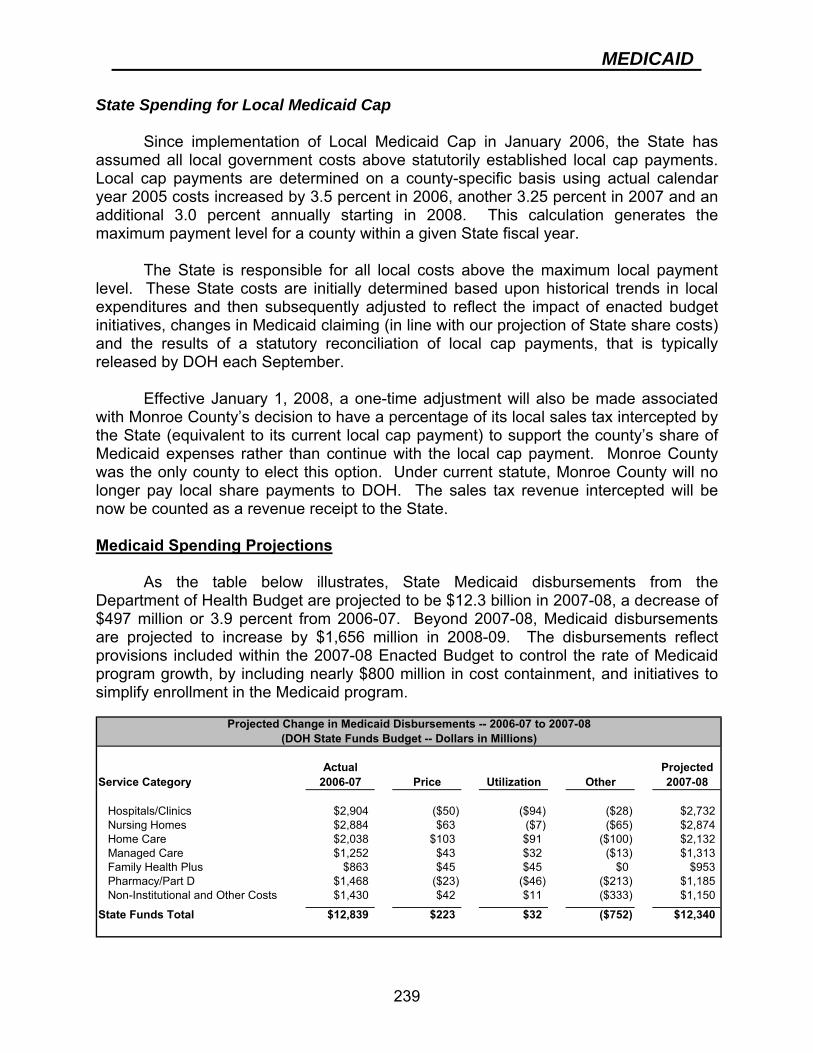
MEDICAID
239
State Spending for Local Medicaid Cap Since implementation of Local Medicaid Cap in January 2006, the State has assumed all local government costs above statutorily established local cap payments. Local cap payments are determined on a county-specific basis using actual calendar year 2005 costs increased by 3.5 percent in 2006, another 3.25 percent in 2007 and an additional 3.0 percent annually starting in 2008. This calculation generates the maximum payment level for a county within a given State fiscal year. The State is responsible for all local costs above the maximum local payment level. These State costs are initially determined based upon historical trends in local expenditures and then subsequently adjusted to reflect the impact of enacted budget initiatives, changes in Medicaid claiming (in line with our projection of State share costs) and the results of a statutory reconciliation of local cap payments, that is typically released by DOH each September. Effective January 1, 2008, a one-time adjustment will also be made associated with Monroe County’s decision to have a percentage of its local sales tax intercepted by the State (equivalent to its current local cap payment) to support the county’s share of Medicaid expenses rather than continue with the local cap payment. Monroe County was the only county to elect this option. Under current statute, Monroe County will no longer pay local share payments to DOH. The sales tax revenue intercepted will be now be counted as a revenue receipt to the State. Medicaid Spending Projections As the table below illustrates, State Medicaid disbursements from the Department of Health Budget are projected to be $12.3 billion in 2007-08, a decrease of $497 million or 3.9 percent from 2006-07. Beyond 2007-08, Medicaid disbursements are projected to increase by $1,656 million in 2008-09. The disbursements reflect provisions included within the 2007-08 Enacted Budget to control the rate of Medicaid program growth, by including nearly $800 million in cost containment, and initiatives to simplify enrollment in the Medicaid program.
Actual ProjectedService Category 2006-07 Price Utilization Other 2007-08
Hospitals/Clinics $2,904 ($50) ($94) ($28) $2,732Nursing Homes $2,884 $63 ($7) ($65) $2,874Home Care $2,038 $103 $91 ($100) $2,132Managed Care $1,252 $43 $32 ($13) $1,313Family Health Plus $863 $45 $45 $0 $953Pharmacy/Part D $1,468 ($23) ($46) ($213) $1,185Non-Institutional and Other Costs $1,430 $42 $11 ($333) $1,150
State Funds Total $12,839 $223 $32 ($752) $12,340
Projected Change in Medicaid Disbursements -- 2006-07 to 2007-08(DOH State Funds Budget -- Dollars in Millions)
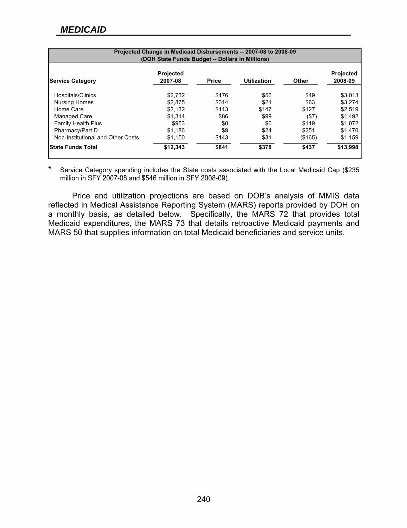
MEDICAID
240
Projected ProjectedService Category 2007-08 Price Utilization Other 2008-09
Hospitals/Clinics $2,732 $176 $56 $49 $3,013Nursing Homes $2,875 $314 $21 $63 $3,274Home Care $2,132 $113 $147 $127 $2,519Managed Care $1,314 $86 $99 ($7) $1,492Family Health Plus $953 $0 $0 $119 $1,072Pharmacy/Part D $1,186 $9 $24 $251 $1,470Non-Institutional and Other Costs $1,150 $143 $31 ($165) $1,159
State Funds Total $12,343 $841 $378 $437 $13,998
Projected Change in Medicaid Disbursements -- 2007-08 to 2008-09(DOH State Funds Budget -- Dollars in Millions)
* Service Category spending includes the State costs associated with the Local Medicaid Cap ($235
million in SFY 2007-08 and $546 million in SFY 2008-09).
Price and utilization projections are based on DOB’s analysis of MMIS data reflected in Medical Assistance Reporting System (MARS) reports provided by DOH on a monthly basis, as detailed below. Specifically, the MARS 72 that provides total Medicaid expenditures, the MARS 73 that details retroactive Medicaid payments and MARS 50 that supplies information on total Medicaid beneficiaries and service units.
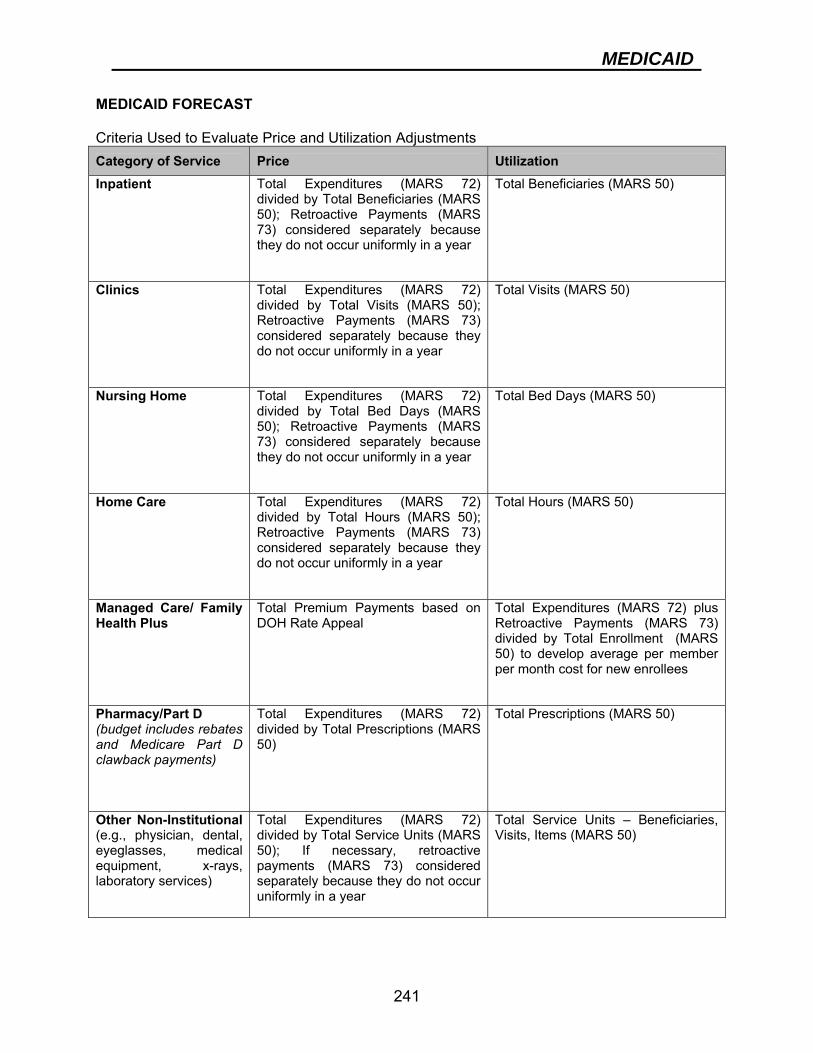
MEDICAID
241
MEDICAID FORECAST Criteria Used to Evaluate Price and Utilization Adjustments Category of Service Price Utilization Inpatient Total Expenditures (MARS 72)
divided by Total Beneficiaries (MARS 50); Retroactive Payments (MARS 73) considered separately because they do not occur uniformly in a year
Total Beneficiaries (MARS 50)
Clinics Total Expenditures (MARS 72) divided by Total Visits (MARS 50); Retroactive Payments (MARS 73) considered separately because they do not occur uniformly in a year
Total Visits (MARS 50)
Nursing Home Total Expenditures (MARS 72) divided by Total Bed Days (MARS 50); Retroactive Payments (MARS 73) considered separately because they do not occur uniformly in a year
Total Bed Days (MARS 50)
Home Care Total Expenditures (MARS 72) divided by Total Hours (MARS 50); Retroactive Payments (MARS 73) considered separately because they do not occur uniformly in a year
Total Hours (MARS 50)
Managed Care/ Family Health Plus
Total Premium Payments based on DOH Rate Appeal
Total Expenditures (MARS 72) plus Retroactive Payments (MARS 73) divided by Total Enrollment (MARS 50) to develop average per member per month cost for new enrollees
Pharmacy/Part D (budget includes rebates and Medicare Part D clawback payments)
Total Expenditures (MARS 72) divided by Total Prescriptions (MARS 50)
Total Prescriptions (MARS 50)
Other Non-Institutional (e.g., physician, dental, eyeglasses, medical equipment, x-rays, laboratory services)
Total Expenditures (MARS 72) divided by Total Service Units (MARS 50); If necessary, retroactive payments (MARS 73) considered separately because they do not occur uniformly in a year
Total Service Units – Beneficiaries, Visits, Items (MARS 50)
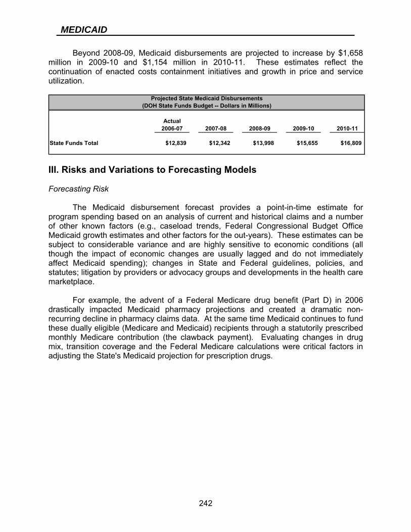
MEDICAID
242
Beyond 2008-09, Medicaid disbursements are projected to increase by $1,658 million in 2009-10 and $1,154 million in 2010-11. These estimates reflect the continuation of enacted costs containment initiatives and growth in price and service utilization.
Actual2006-07 2007-08 2008-09 2009-10 2010-11
State Funds Total $12,839 $12,342 $13,998 $15,655 $16,809
Projected State Medicaid Disbursements(DOH State Funds Budget -- Dollars in Millions)
III. Risks and Variations to Forecasting Models Forecasting Risk The Medicaid disbursement forecast provides a point-in-time estimate for program spending based on an analysis of current and historical claims and a number of other known factors (e.g., caseload trends, Federal Congressional Budget Office Medicaid growth estimates and other factors for the out-years). These estimates can be subject to considerable variance and are highly sensitive to economic conditions (all though the impact of economic changes are usually lagged and do not immediately affect Medicaid spending); changes in State and Federal guidelines, policies, and statutes; litigation by providers or advocacy groups and developments in the health care marketplace.
For example, the advent of a Federal Medicare drug benefit (Part D) in 2006 drastically impacted Medicaid pharmacy projections and created a dramatic non-recurring decline in pharmacy claims data. At the same time Medicaid continues to fund these dually eligible (Medicare and Medicaid) recipients through a statutorily prescribed monthly Medicare contribution (the clawback payment). Evaluating changes in drug mix, transition coverage and the Federal Medicare calculations were critical factors in adjusting the State's Medicaid projection for prescription drugs.
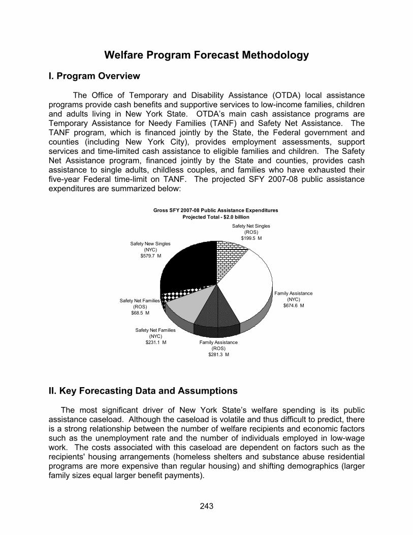
243
Welfare Program Forecast Methodology I. Program Overview
The Office of Temporary and Disability Assistance (OTDA) local assistance programs provide cash benefits and supportive services to low-income families, children and adults living in New York State. OTDA’s main cash assistance programs are Temporary Assistance for Needy Families (TANF) and Safety Net Assistance. The TANF program, which is financed jointly by the State, the Federal government and counties (including New York City), provides employment assessments, support services and time-limited cash assistance to eligible families and children. The Safety Net Assistance program, financed jointly by the State and counties, provides cash assistance to single adults, childless couples, and families who have exhausted their five-year Federal time-limit on TANF. The projected SFY 2007-08 public assistance expenditures are summarized below:
Gross SFY 2007-08 Public Assistance Expenditures
Projected Total - $2.0 billionSafety Net Singles
(ROS)$199.5 M
Family Assistance (NYC)
$674.6 M
Family Assistance (ROS)
$281.3 M
Safety Net Families (NYC)
$231.1 M
Safety New Singles (NYC)
$579.7 M
Safety Net Families (ROS)
$68.5 M
II. Key Forecasting Data and Assumptions
The most significant driver of New York State’s welfare spending is its public assistance caseload. Although the caseload is volatile and thus difficult to predict, there is a strong relationship between the number of welfare recipients and economic factors such as the unemployment rate and the number of individuals employed in low-wage work. The costs associated with this caseload are dependent on factors such as the recipients' housing arrangements (homeless shelters and substance abuse residential programs are more expensive than regular housing) and shifting demographics (larger family sizes equal larger benefit payments).
WELFARE
244
The welfare model provides forecasts for TANF families and Safety Net recipients separately for New York City (NYC) and for the rest of the State (ROS). ROS includes rural upstate and western New York as well as the wealthier, more densely populated suburban counties of the Hudson Valley and Long Island. The forecast for TANF families includes those families that have exhausted their five-year Federal time-limit (Safety Net families).
Current Population Survey data indicate that welfare recipients who work tend to be concentrated in industries that have large numbers of relatively low-wage entry level jobs. For convenience, we refer to employment aggregated across these industries as “entry-level employment.” Additional factors believed to be relevant to labor market entry include unemployment rates, the level of the minimum wage, and the size of the Earned Income Tax Credit (EITC) - a refundable credit aimed at low-income working families with children.
DOB uses econometric models to forecast entry-level employment and unemployment rates separately for NYC and for ROS. Many of the input variables used in these models, such as statewide unemployment rates, statewide employment in entry-level industries, and real wages in the finance and insurance sector, are derived from DOB’s macroeconomic model for the New York State economy. In a second set of econometric models, welfare caseloads are estimated conditional on the forecasts for entry-level employment levels, unemployment rates, and other relevant variables. Thus, the caseload forecasts are fully consistent with DOB’s overall economic outlook. A) Forecasting Regional Employment and Unemployment Rates
Entry-level employment is defined here as employment aggregated over the following sectors: manufacturing; retail trade; administrative and support and waste management and remediation services; arts, entertainment, and recreation; accommodation and food services; and other services. Regional entry-level employment is assumed to be driven by the same factors that drive statewide employment growth in those same industries. Statewide entry-level employment growth is used as a proxy for those factors.
Estimation results suggest that a one-percent increase in statewide entry-level employment increases NYC entry-level employment by about 1.3 percent and ROS entry-level employment by 0.9 percent. Growth in ROS entry-level employment is also lifted by wage growth in the finance and insurance sector, though with a lag. Finance and insurance sector wages have a large spillover effect onto the rest of the State economy as commuters spend their incomes in their counties of residence.
Estimation results also indicate that a one-percentage point increase in the statewide unemployment rate is predicted to increase the NYC unemployment rate by about 1.1 percentage points, while a one-percent increase in finance and insurance industry wages is estimated to increase the NYC unemployment rate by 0.07 percentage points with a lag. A one-percentage point rise in the State’s unemployment
WELFARE
245
rate is estimated to increase the ROS unemployment rate by about 0.9 percentage points. B) Forecasting Welfare Caseloads
Table 1 shows the specifications for the welfare caseload equations.28 Caseloads are estimated to vary with entry-level employment levels and unemployment rates, as well as with various measures related to compensation deemed particularly relevant for entry-level workers. These measures include the statewide average nonfarm wage, the State minimum wage level, and the EITC. The models also contain measures that attempt to capture the impact of administrative and programmatic efforts at the national, State, and local levels to reduce welfare dependency, including changes in eligibility criteria such as the added work requirements and term limits introduced with the passage of the Federal Personal Responsibility and Work Opportunity Reconciliation Act of 1996 (PRWORA) - which replaced the old welfare program.
Growth in the New York City TANF population is a function of the prior quarter’s TANF population and the impact of local and State administrative efforts lasting from the first quarter of 1995 through the third quarter of 2001.29 In addition, an increase in statewide nonfarm wage growth is estimated to result in a decrease in caseload growth with a two-quarter lag. Higher NYC entry-level employment levels are estimated to reduce caseloads five quarters later.
Changes in the minimum wage rate and the maximum EITC benefit also have an impact on TANF caseloads in New York City, though the magnitude of these impacts appears to have changed with the introduction of work requirements and term limits under PRWORA. Starting in the first quarter of 1997, a one-percent increase in the minimum wage is estimated to reduce the NYC caseload by about 0.08 percent. This result suggests that during the period since welfare reform, the incentive for welfare recipients to find work when the minimum wage increases overrides employers’ incentive to reduce their demand for workers in response to higher labor costs. Prior to welfare reform, a one-percent increase in the minimum wage actually raised the welfare caseload by about 0.06 percent. Similarly, a one-percent increase in the maximum EITC benefit amount is estimated to lower the NYC TANF caseload as of the beginning of 1997, while having virtually no impact prior to that year.
The TANF caseload growth for the rest of the state also depends on its own past value, past values of ROS entry-level employment growth, and administrative efforts. Changes in both the maximum EITC benefit and the minimum wage fail to have a significant impact on ROS caseloads.
28 In this report, the “caseload” is defined as the number of recipients. 29 The estimated endpoint for these efforts is presumed to coincide with the terrorist attacks of September 11.
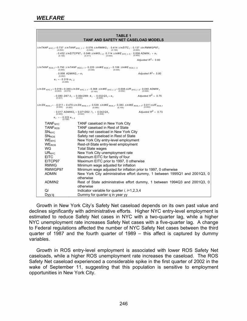
WELFARE
246
TABLE 1
TANF AND SAFETY NET CASELOAD MODELS
TANFNYC TANF caseload in New York City TANFROS TANF caseload in Rest of State SNNYC Safety net caseload in New York City SNROS Safety net caseload in Rest of State WENYC New York City entry-level employment WEROS Rest-of-State entry-level employment WG Total State wages URNYC New York City unemployment rate EITC Maximum EITC for family of four EITCP97 Maximum EITC prior to 1997, 0 otherwise RMWG Minimum wage adjusted for inflation RMWGP97 Minimum wage adjusted for inflation prior to 1997, 0 otherwise ADMIN New York City administrative effort dummy, 1 between 1995Q1 and 2001Q3, 0
otherwise ADMIN2 Rest of State administrative effort dummy, 1 between 1994Q3 and 2001Q3, 0
otherwise Qi Indicator variable for quarter i, i=1,2,3,4 Dyy:q Dummy for quarter q in year yy
Growth in New York City’s Safety Net caseload depends on its own past value and
declines significantly with administrative efforts. Higher NYC entry-level employment is estimated to reduce Safety Net cases in NYC with a two-quarter lag, while a higher NYC unemployment rate increases Safety Net cases with a five-quarter lag. A change to Federal regulations affected the number of NYC Safety Net cases between the third quarter of 1987 and the fourth quarter of 1989 – this affect is captured by dummy variables.
Growth in ROS entry-level employment is associated with lower ROS Safety Net
caseloads, while a higher ROS unemployment rate increases the caseload. The ROS Safety Net caseload experienced a considerable spike in the first quarter of 2002 in the wake of September 11, suggesting that this population is sensitive to employment opportunities in New York City.
− − +−
+ − −− −
=
−
Δ Δ Δ Δ Δ
Δ Δ Δ +
NYC t NYC t t t t
t t NYC t t t
TANF TANF RMWG EITC RMWGP
EITCP WG WE ADMIN e
Adj
, , 1(0.052) (0.040) (0.109) (0.065)
2 , 5(0.002)(0.109) (0.011) (0.044)
ln 0.737 ln 0.076 ln 0.414 ln 0.137 ln 97
0.432 ln 97 0.046 ln 0.114 ln 0.008
− −
−
−
=
Δ = Δ − Δ − Δ
+ =
=−
Δ = + Δ
ROS t ROS t ROS t ROS t
t t
t t
NYC t NY
usted R
TANF TANF WE WE
ADMIN e Adjusted R
e e
SN SN
, , 1 , , 3(0.055) (0.036) (0.036)
2
(0.002)
2(0.099)
, (0.003) (0.075)
2 0.80
ln 0.750 ln 0.220 ln 0.106 ln
0.008 2 0.80
0.319
ln 0.018 0.340 ln − − −
−
− Δ + Δ −
− + − + =
Δ = − + Δ −
C t NYC t NYC t t
t t t t
ROS t ROS t
WE UR ADMIN
D87:3 D Q e Adjusted R
SN SN
, 1 , 2 , 5(0.002) (0.006)(0.163)
(0.021) (0.020) (0.009)
, , 1(0.004) (0.082)
2
0.368 ln 0.008 0.040
0.080 0.064 89 : 4 0.032 3 0.75
ln 0.011 0.470 ln 0.53 −
−
Δ − Δ + Δ
− + + =
= −
ROS t ROS t ROS t
t t t
t t
WE WE UR
ADMIN D Q Adjusted R
e e
, , 1 ,(0.004)(0.080) (0.105)
(0.005) (0.022) (0.009)
2(0.109)
2
9 ln 0.383 ln 0.011
0.017 2 0.071 02 : 1 0.042 4 0.73
0.222
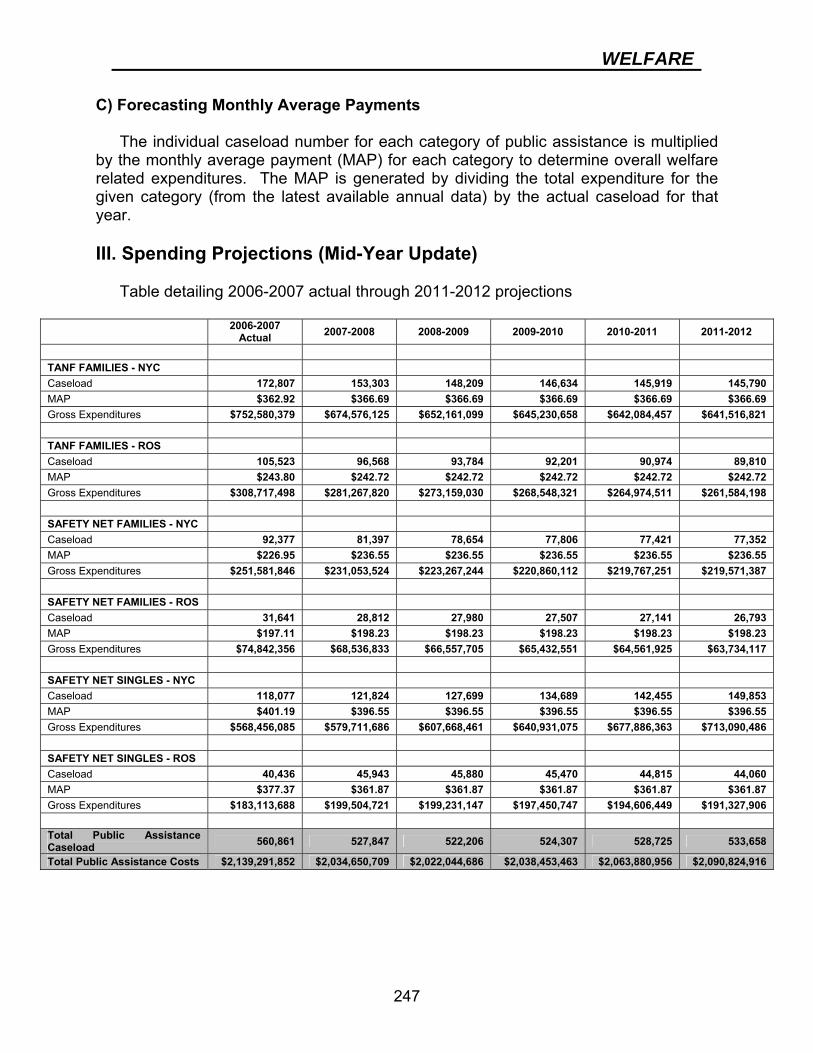
WELFARE
247
C) Forecasting Monthly Average Payments
The individual caseload number for each category of public assistance is multiplied by the monthly average payment (MAP) for each category to determine overall welfare related expenditures. The MAP is generated by dividing the total expenditure for the given category (from the latest available annual data) by the actual caseload for that year. III. Spending Projections (Mid-Year Update)
Table detailing 2006-2007 actual through 2011-2012 projections
2006-2007 Actual 2007-2008 2008-2009 2009-2010 2010-2011 2011-2012
TANF FAMILIES - NYC Caseload 172,807 153,303 148,209 146,634 145,919 145,790 MAP $362.92 $366.69 $366.69 $366.69 $366.69 $366.69 Gross Expenditures $752,580,379 $674,576,125 $652,161,099 $645,230,658 $642,084,457 $641,516,821 TANF FAMILIES - ROS Caseload 105,523 96,568 93,784 92,201 90,974 89,810 MAP $243.80 $242.72 $242.72 $242.72 $242.72 $242.72 Gross Expenditures $308,717,498 $281,267,820 $273,159,030 $268,548,321 $264,974,511 $261,584,198 SAFETY NET FAMILIES - NYC Caseload 92,377 81,397 78,654 77,806 77,421 77,352 MAP $226.95 $236.55 $236.55 $236.55 $236.55 $236.55 Gross Expenditures $251,581,846 $231,053,524 $223,267,244 $220,860,112 $219,767,251 $219,571,387 SAFETY NET FAMILIES - ROS Caseload 31,641 28,812 27,980 27,507 27,141 26,793 MAP $197.11 $198.23 $198.23 $198.23 $198.23 $198.23 Gross Expenditures $74,842,356 $68,536,833 $66,557,705 $65,432,551 $64,561,925 $63,734,117 SAFETY NET SINGLES - NYC Caseload 118,077 121,824 127,699 134,689 142,455 149,853 MAP $401.19 $396.55 $396.55 $396.55 $396.55 $396.55 Gross Expenditures $568,456,085 $579,711,686 $607,668,461 $640,931,075 $677,886,363 $713,090,486 SAFETY NET SINGLES - ROS Caseload 40,436 45,943 45,880 45,470 44,815 44,060 MAP $377.37 $361.87 $361.87 $361.87 $361.87 $361.87 Gross Expenditures $183,113,688 $199,504,721 $199,231,147 $197,450,747 $194,606,449 $191,327,906 Total Public Assistance Caseload 560,861 527,847 522,206 524,307 528,725 533,658
Total Public Assistance Costs $2,139,291,852 $2,034,650,709 $2,022,044,686 $2,038,453,463 $2,063,880,956 $2,090,824,916

WELFARE
248
IV. Risks and Variations to Forecasting Model
A major risk factor in the welfare caseload forecast entails using monthly average payments that are one year old in the projection of future costs– the alternative would be to trend MAP for each category of public assistance. However, due to the variances in the growth patterns of these different groups, trending would most likely result in inflated projections. In addition to the MAP issue, there are numerous other factors that can impact costs, from a sudden downturn in the economy to policy and/or administrative changes that make it easier to become eligible for or remain on public assistance.
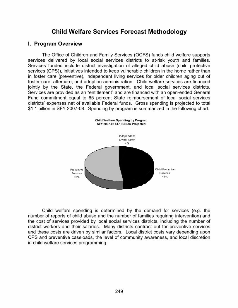
249
Child Welfare Spending by ProgramSFY 2007-08 $1.1 Billion Projected
Independent Living, Other
4%
Child Protective Services
44%
Preventive Services
52%
Child Welfare Services Forecast Methodology I. Program Overview The Office of Children and Family Services (OCFS) funds child welfare supports services delivered by local social services districts to at-risk youth and families. Services funded include district investigation of alleged child abuse (child protective services (CPS)), initiatives intended to keep vulnerable children in the home rather than in foster care (preventive), independent living services for older children aging out of foster care, aftercare, and adoption administration. Child welfare services are financed jointly by the State, the Federal government, and local social services districts. Services are provided as an “entitlement” and are financed with an open-ended General Fund commitment equal to 65 percent State reimbursement of local social services districts’ expenses net of available Federal funds. Gross spending is projected to total $1.1 billion in SFY 2007-08. Spending by program is summarized in the following chart:
Child welfare spending is determined by the demand for services (e.g. the number of reports of child abuse and the number of families requiring intervention) and the cost of services provided by local social services districts, including the number of district workers and their salaries. Many districts contract out for preventive services and these costs are driven by similar factors. Local district costs vary depending upon CPS and preventive caseloads, the level of community awareness, and local discretion in child welfare services programming.
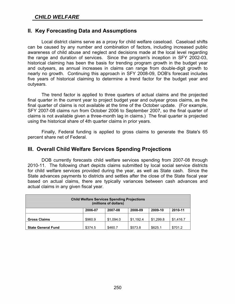
CHILD WELFARE
250
II. Key Forecasting Data and Assumptions Local district claims serve as a proxy for child welfare caseload. Caseload shifts can be caused by any number and combination of factors, including increased public awareness of child abuse and neglect and decisions made at the local level regarding the range and duration of services. Since the program's inception in SFY 2002-03, historical claiming has been the basis for trending program growth in the budget year and outyears, as annual increases in claims can range from double-digit growth to nearly no growth. Continuing this approach in SFY 2008-09, DOB's forecast includes five years of historical claiming to determine a trend factor for the budget year and outyears. The trend factor is applied to three quarters of actual claims and the projected final quarter in the current year to project budget year and outyear gross claims, as the final quarter of claims is not available at the time of the October update. (For example, SFY 2007-08 claims run from October 2006 to September 2007, so the final quarter of claims is not available given a three-month lag in claims.) The final quarter is projected using the historical share of 4th quarter claims in prior years. Finally, Federal funding is applied to gross claims to generate the State's 65 percent share net of Federal. III. Overall Child Welfare Services Spending Projections DOB currently forecasts child welfare services spending from 2007-08 through 2010-11. The following chart depicts claims submitted by local social service districts for child welfare services provided during the year, as well as State cash. Since the State advances payments to districts and settles after the close of the State fiscal year based on actual claims, there are typically variances between cash advances and actual claims in any given fiscal year.
Child Welfare Services Spending Projections
(millions of dollars)
2006-07 2007-08 2008-09 2009-10 2010-11
Gross Claims $960.9 $1,094.0 $1,192.4 $1,299.8 $1,416.7
State General Fund $374.5 $460.7 $573.8 $625.1 $701.2

CHILD WELFARE
251
IV. Risks in Child Welfare Services Forecast Local district claiming is generally difficult to predict. Claiming patterns are affected by: the lack of predictability in service utilization as districts vary in their responses to child welfare service needs; varying individual service needs and costs; districts' flexibility to submit claims long after the close of a fiscal year, leaving open the final settlement of the year (addressed in SFY 2007-08 through implementation of local district claiming deadlines in 07-08 and beyond); and variances in the financial capacity of districts to invest in child welfare services as districts must first invest in programs and then receive reimbursement. While program volatility is mitigated by the use of historical trends to project future expenditures, large swings in claims and sudden environmental changes (e.g.; a high profile child abuse case that prompts additional reporting) are difficult to anticipate.
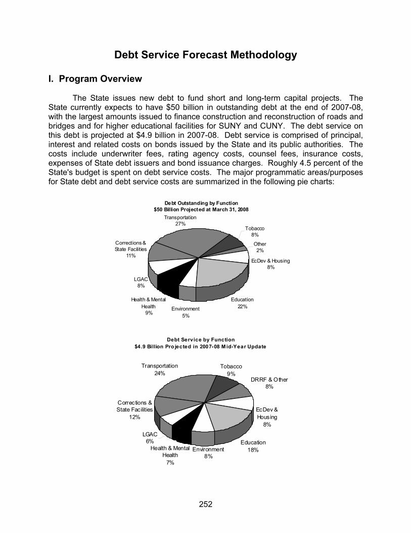
252
Debt Service Forecast Methodology
I. Program Overview The State issues new debt to fund short and long-term capital projects. The
State currently expects to have $50 billion in outstanding debt at the end of 2007-08, with the largest amounts issued to finance construction and reconstruction of roads and bridges and for higher educational facilities for SUNY and CUNY. The debt service on this debt is projected at $4.9 billion in 2007-08. Debt service is comprised of principal, interest and related costs on bonds issued by the State and its public authorities. The costs include underwriter fees, rating agency costs, counsel fees, insurance costs, expenses of State debt issuers and bond issuance charges. Roughly 4.5 percent of the State's budget is spent on debt service costs. The major programmatic areas/purposes for State debt and debt service costs are summarized in the following pie charts:
Debt Outstanding by Function$50 Billion Projected at March 31, 2008
Education22%
Corrections & State Facilities
11%
Tobacco8%
Health & Mental Health
9%
Transportation27%
Other2%
EcDev & Housing8%
LGAC 8%
Environment5%
Debt Service by Function$4.9 Billion Pro jected in 2007-08 M id-Year Update
Education18%Health & Mental
Health7%
LGAC 6%
Transportation24%
EcDev & Housing
8%
Corrections & State Facilities
12%
DRRF & Other8%
Environment8%
Tobacco9%
DEBT SERVICE
253
DOB prepares a detailed five-year projection of State debt levels and related
costs twice annually, including all the major areas of existing and planned debt levels. This information (the “Capital Program and Financing Plan”) is available on the DOB website (www.budget.state.ny.us) and is provided with the Executive and Enacted Budgets and major data is updated quarterly with each Financial Plan Update.
II. Overview of Debt Service Forecast
The DOB uses a multi-faceted approach to forecast debt service costs as described in detail below. This includes forecasts for both fixed and variable interest rate costs and projections for the amount of new fixed and variable rate debt that is planned to be issued to finance capital projects over the next five year period.
The State makes annual payments of roughly equal amounts over the life of a
bond-financing (“level debt service”), similar to the repayment terms of a typical home mortgage. Therefore, the State’s annual costs for an individual bond financing generally remain the same each year until the debt is retired, with greater interest payments occurring in the earlier years and greater principal payments in the later years.
Many consider debt service to be a “fixed” cost. In reality, debt service costs can
change relatively quickly, and are affected by legislation that determines both the size of capital projects and whether the capital projects will be debt-financed (which drives future debt service costs) or “pay-as-you-go” where current resources are used to finance capital spending and no debt service costs result. For example, in the current fiscal year, virtually the entire amount of State-related debt service is for the payment of bonds issued in prior years. By 2011-12, based on the current forecast, that share will drop to 70 percent of the projected State debt service in that year. To a lesser extent, debt service costs fluctuate due to the impact of refundings (which lower existing debt service costs), movements in interest rates for variable rate debt, changes in the demand for State debt, and other market dynamics.
The debt service forecast is comprised of two distinct, but related, components
(1) the costs for debt obligations that have already been issued and (2) the projected new debt service costs for bonds that have yet to be issued to finance capital projects authorized by legislation. The debt service forecast is less likely to vary significantly for debt that has already been issued, and more subject to change for debt that has not yet been issued. The different factors affecting each category are summarized below.
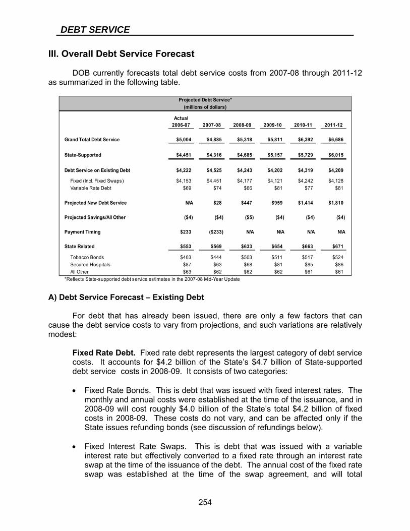
DEBT SERVICE
254
III. Overall Debt Service Forecast DOB currently forecasts total debt service costs from 2007-08 through 2011-12
as summarized in the following table.
A) Debt Service Forecast – Existing Debt
For debt that has already been issued, there are only a few factors that can cause the debt service costs to vary from projections, and such variations are relatively modest:
Fixed Rate Debt. Fixed rate debt represents the largest category of debt service costs. It accounts for $4.2 billion of the State’s $4.7 billion of State-supported debt service costs in 2008-09. It consists of two categories:
• Fixed Rate Bonds. This is debt that was issued with fixed interest rates. The
monthly and annual costs were established at the time of the issuance, and in 2008-09 will cost roughly $4.0 billion of the State’s total $4.2 billion of fixed costs in 2008-09. These costs do not vary, and can be affected only if the State issues refunding bonds (see discussion of refundings below).
• Fixed Interest Rate Swaps. This is debt that was issued with a variable interest rate but effectively converted to a fixed rate through an interest rate swap at the time of the issuance of the debt. The annual cost of the fixed rate swap was established at the time of the swap agreement, and will total
Actual 2006-07 2007-08 2008-09 2009-10 2010-11 2011-12
Grand Total Debt Service $5,004 $4,885 $5,318 $5,811 $6,392 $6,686
State-Supported $4,451 $4,316 $4,685 $5,157 $5,729 $6,015
Debt Service on Existing Debt $4,222 $4,525 $4,243 $4,202 $4,319 $4,209
Fixed (Incl. Fixed Swaps) $4,153 $4,451 $4,177 $4,121 $4,242 $4,128 Variable Rate Debt $69 $74 $66 $81 $77 $81
Projected New Debt Service N/A $28 $447 $959 $1,414 $1,810
Projected Savings/All Other ($4) ($4) ($5) ($4) ($4) ($4)
Payment Timing $233 ($233) N/A N/A N/A N/A
State Related $553 $569 $633 $654 $663 $671
Tobacco Bonds $403 $444 $503 $511 $517 $524 Secured Hospitals $87 $63 $68 $81 $85 $86 All Other $63 $62 $62 $62 $61 $61*Reflects State-supported debt service estimates in the 2007-08 Mid-Year Update
Projected Debt Service*(millions of dollars)
DEBT SERVICE
255
roughly $222 million of the $4.2 billion of fixed costs in 2008-09. Although the State pays a fixed swap rate and this cost is known, there can be a difference between the variable rates paid to bondholders and the variable rate received from swap counterparties by the State. The “basis risk” between these variable rates used to hedge each other is accounted for in the variable rate projections discussed below. Based on past experience, this difference is not significant (in 2006-07, the State received $2 million more than it paid).30
Variable Rate Debt. Another potential variance from the forecast for existing debt is that actual interest rates will vary on the roughly $2.5 billion of net variable rate debt that has been previously issued. Such variable rate costs also include the basis risk discussed earlier. The variable rate debt service costs are projected to total $66 million in 2008-09 based primarily on a projected 3.3 percent tax exempt interest rate, 25 basis points less than in 2007-08.
While changes in variable rate debt costs can impact debt service costs, they create little significant overall Financial Plan impact since the variation is typically offset by the amount of revenue received from interest earnings on the State’s short term assets (the Short-Term Investment Pool “STIP”). The earnings on STIP will typically move in the same direction as the variable rate debt service costs. If interest rates rise, the State’s interest revenues increase from higher STIP earnings which offsets the State’s higher debt service costs (and vice versa), such that there is little material risk to the State’s overall financial plan. The State’s variable rate policy and statutory limits are designed to balance these risks, and are described in detail on the DOB website.
B) Debt Service Forecast – New Debt
Some aspects for projecting new debt service costs are relatively clear, including the amount of debt that is statutorily authorized to be issued and the total amount of bond-financed capital spending that is statutorily authorized to be spent.
But some aspects are less clear until more specific information becomes
available about the authorized capital projects, including:
• Whether certain types of capital projects are eligible for lower cost tax-exempt financing or require more expensive taxable financing.
• The length of time the debt will be outstanding (e.g., 10 years or 30 years),
which is primarily determined by the useful life of the projects being financed.
• The timing of annual spending for each of the approved capital projects which typically “ramp up” over a multi-year period (e.g., the State is still spending for General Obligation capital projects approved by the voters in the 1980s).
30 See the DOB website for more information on interest rate swaps, policies, statutory limits and performance, including a comprehensive report of the State’s swap portfolio issued on October 30, 2007.
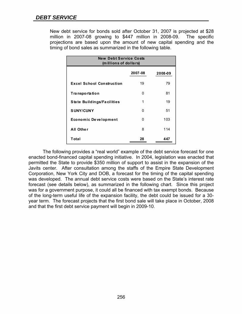
DEBT SERVICE
256
New debt service for bonds sold after October 31, 2007 is projected at $28 million in 2007-08 growing to $447 million in 2008-09. The specific projections are based upon the amount of new capital spending and the timing of bond sales as summarized in the following table.
The following provides a “real world” example of the debt service forecast for one enacted bond-financed capital spending initiative. In 2004, legislation was enacted that permitted the State to provide $350 million of support to assist in the expansion of the Javits center. After consultation among the staffs of the Empire State Development Corporation, New York City and DOB, a forecast for the timing of the capital spending was developed. The annual debt service costs were based on the State’s interest rate forecast (see details below), as summarized in the following chart. Since this project was for a government purpose, it could all be financed with tax exempt bonds. Because of the long-term useful life of the expansion facility, the debt could be issued for a 30-year term. The forecast projects that the first bond sale will take place in October, 2008 and that the first debt service payment will begin in 2009-10.
2007-08 2008-09
Excel School Construction 19 79
Tra nsporta tion 0 81
Sta te Buildings/Fa cilities 1 19
SUNY/CUNY 0 51
Economic De ve lopment 0 103
All Othe r 8 114
Total 28 447
New Debt Service Costs(m illions of dolla rs)
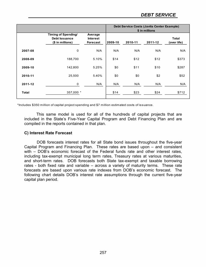
DEBT SERVICE
257
This same model is used for all of the hundreds of capital projects that are
included in the State’s Five-Year Capital Program and Debt Financing Plan and are compiled in the reports contained in that plan. C) Interest Rate Forecast
DOB forecasts interest rates for all State bond issues throughout the five-year Capital Program and Financing Plan. These rates are based upon – and consistent with – DOB’s economic forecast of the Federal funds rate and other interest rates, including tax-exempt municipal long term rates, Treasury rates at various maturities, and short-term rates. DOB forecasts both State tax-exempt and taxable borrowing rates - both fixed rate and variable – across a variety of maturity terms. These rate forecasts are based upon various rate indexes from DOB’s economic forecast. The following chart details DOB’s interest rate assumptions through the current five-year capital plan period.
Timing of Spending/Debt Issuance ($ in millions)
Average Interest Forecast 2009-10 2010-11 2011-12
Total(over life)
2007-08 0 N/A N/A N/A N/A N/A
2008-09 188,700 5.10% $14 $12 $12 $373
2009-10 142,800 5.25% $0 $11 $10 $287
2010-11 25,500 5.40% $0 $0 $2 $52
2011-12 0 N/A N/A N/A N/A N/A
Total 357,000 * $14 $23 $24 $712
*Includes $350 million of capital project spending and $7 million estimated costs of issuance.
Debt Service Costs (Javits Center Example)$ in millions
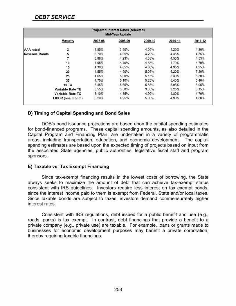
DEBT SERVICE
258
D) Timing of Capital Spending and Bond Sales
DOB’s bond issuance projections are based upon the capital spending estimates for bond-financed programs. These capital spending amounts, as also detailed in the Capital Program and Financing Plan, are undertaken in a variety of programmatic areas, including transportation, education, and economic development. The capital spending estimates are based upon the expected timing of projects based on input from the associated State agencies, public authorities, legislative fiscal staff and program sponsors. E) Taxable vs. Tax Exempt Financing
Since tax-exempt financing results in the lowest costs of borrowing, the State always seeks to maximize the amount of debt that can achieve tax-exempt status consistent with IRS guidelines. Investors require less interest on tax exempt bonds, since the interest income paid to them is exempt from Federal, State and/or local taxes. Since taxable bonds are subject to taxes, investors demand commensurately higher interest rates.
Consistent with IRS regulations, debt issued for a public benefit and use (e.g.,
roads, parks) is tax exempt. In contrast, debt financings that provide a benefit to a private company (e.g., private use) are taxable. For example, loans or grants made to businesses for economic development purposes may benefit a private corporation, thereby requiring taxable financings.
Maturity 2007-08 2008-09 2009-10 2010-11 2011-12
AAA-rated 3 3.55% 3.90% 4.05% 4.20% 4.20%Revenue Bonds 5 3.70% 4.05% 4.20% 4.35% 4.35%
7 3.88% 4.23% 4.38% 4.53% 4.53%10 4.05% 4.40% 4.55% 4.70% 4.70%15 4.30% 4.65% 4.80% 4.95% 4.95%20 4.55% 4.90% 5.05% 5.20% 5.20%25 4.65% 5.00% 5.15% 5.30% 5.30%30 4.75% 5.10% 5.25% 5.40% 5.40%
10 TX 5.45% 5.65% 5.85% 5.95% 5.95%Variable Rate TE 3.55% 3.30% 3.35% 3.25% 3.15%Variable Rate TX 5.10% 4.85% 4.90% 4.80% 4.70%
LIBOR (one month) 5.20% 4.95% 5.00% 4.90% 4.80%
Projected Interest Rates (selected)Mid-Year Update
DEBT SERVICE
259
F) Bond Maturities
State-related debt is issued with maturities based upon the useful life of the capital project being financed, with a maximum term of 30 years for tax exempt debt and 10 years for taxable borrowings. The maturities vary for each bond sale depending on the specific component programs and projects that are being financed. Generally, debt maturities for ongoing projects are as follows:
• Transportation – 20 years • Higher Education (SUNY and CUNY) - 30 years • Mental Health – various up to 30 years • Environment – 20 years • Correctional Facilities – 30 years • State office buildings and other facilities – primarily 20 years • Housing programs - 30 years • Economic development – 20 years • Equipment purposes – generally 3 to 5 years • Taxable Debt - maximum term – 10 years
G) Projected Savings/All Other
The current debt service forecast incorporates projected savings associated with
a variety of legislatively-enacted and administrative debt management initiatives. Generally, these savings are based on expected bond performance, refunding opportunities, and negotiations with legislative fiscal committees as part of the Enacted Budget. Most of the savings target results from potential refunding opportunities. With refundings, the State effectively replaces higher interest rate debt with lower cost debt, which is dependent on current market interest rates and compliance with DOB’s refunding criteria encompassed in its debt policies. (The debt policies are described in detail on the DOB website.)
In addition, the projections incorporate the fiscal impacts of support costs for
variable rate debt, bond trustee fees, public authority fees associated with their staff costs for administering the State’s debt programs and interest earnings on bond proceeds, consistent with IRS limitations.
H) Payment Timing
Debt service payments are scheduled to be made to bond trustees pursuant to contractual commitments made at the time of each bond sale. In certain circumstances, usually related to earlier than expected processing of paperwork, payments are made sooner than originally planned. For example, at the end of 2006-07 $233 million of payments were made on March 27 that were originally scheduled for early April. These timing changes have no impact on ultimate total debt service costs, but sometimes impact cash-basis results in a given fiscal year.
DEBT SERVICE
260
IV. Variation in Forecast As discussed previously, only a relatively small portion of the State’s debt service
spending forecast is subject to change since most of the costs are based on debt that has already been issued in a fixed rate mode. However, over time, bonds that are projected to be issued comprise a growing portion of the State’s debt service spending.
The two key elements that have the greatest potential to result in variances from
the projected annual level of debt service costs are (1) the timing of new capital spending in each fiscal year, and the resultant timing and amount of new bond sales and (2) the interest rate forecast, including whether rates are above or below projected levels, with the most immediate impact felt on variable rate bonds.
In terms of the interest rate forecast:
• An increase or decrease of one percent in variable interest rates from DOB’s
current forecast (from 3.3 percent to either 2.3 percent or 4.3 percent for tax exempt debt) would result in a $40 million variance from 2008-09 projections.
• The impact of a consistent 1 percent change from DOB’s projected fixed interest rate forecast (for example, from 5.10 percent to either 4.10 percent or 6.10 percent for 30-year tax exempt debt in 2008-09) has a cumulatively larger impact with each subsequent fiscal year – from $33 million in 2008-09 to $147 million by 2011-12.
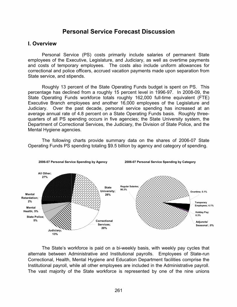
261
Personal Service Forecast Discussion I. Overview
Personal Service (PS) costs primarily include salaries of permanent State employees of the Executive, Legislature, and Judiciary, as well as overtime payments and costs of temporary employees. The costs also include uniform allowances for correctional and police officers, accrued vacation payments made upon separation from State service, and stipends.
Roughly 13 percent of the State Operating Funds budget is spent on PS. This percentage has declined from a roughly 15 percent level in 1996-97. In 2008-09, the State Operating Funds workforce totals roughly 162,000 full-time equivalent (FTE) Executive Branch employees and another 16,000 employees of the Legislature and Judiciary. Over the past decade, personal service spending has increased at an average annual rate of 4.8 percent on a State Operating Funds basis. Roughly three-quarters of all PS spending occurs in five agencies; the State University system, the Department of Correctional Services, the Judiciary, the Division of State Police, and the Mental Hygiene agencies.
The following charts provide summary data on the shares of 2006-07 State
Operating Funds PS spending totaling $9.5 billion by agency and category of spending.
The State’s workforce is paid on a bi-weekly basis, with weekly pay cycles that alternate between Administrative and Institutional payrolls. Employees of State-run Correctional, Health, Mental Hygiene and Education Department facilities comprise the Institutional payroll, while all other employees are included in the Administrative payroll. The vast majority of the State workforce is represented by one of the nine unions
2006-07 Personal Service Spending by Agency
Regular Salaries; 90.3%
Adjuncts/Seasonal ; 0%
Holiday Pay; 0.3%
Overtime; 5.1%
Temporary Employees; 4.1%
2006-07 Personal Service Spending by Category
All Other; 27%
Mental Retardation;
2%
Mental Health; 5%
State Police; 5%
Judiciary; 13%
Correctional Services;
20%
State University;
28%
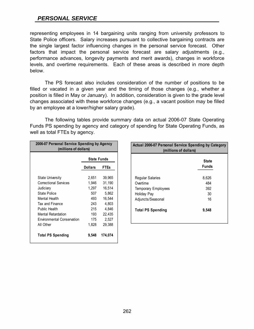
PERSONAL SERVICE
262
representing employees in 14 bargaining units ranging from university professors to State Police officers. Salary increases pursuant to collective bargaining contracts are the single largest factor influencing changes in the personal service forecast. Other factors that impact the personal service forecast are salary adjustments (e.g., performance advances, longevity payments and merit awards), changes in workforce levels, and overtime requirements. Each of these areas is described in more depth below.
The PS forecast also includes consideration of the number of positions to be filled or vacated in a given year and the timing of those changes (e.g., whether a position is filled in May or January). In addition, consideration is given to the grade level changes associated with these workforce changes (e.g., a vacant position may be filled by an employee at a lower/higher salary grade).
The following tables provide summary data on actual 2006-07 State Operating Funds PS spending by agency and category of spending for State Operating Funds, as well as total FTEs by agency.
State Funds
Regular Salaries 8,626 Overtime 484 Temporary Employees 392 Holiday Pay 30 Adjuncts/Seasonal 16
Total PS Spending 9,548
Actual 2006-07 Personal Service Spending by Category(millions of dollars)
Dollars FTEs
State University 2,651 39,965 Correctional Services 1,946 31,190 Judiciary 1,297 16,514 State Police 507 5,862 Mental Health 493 16,544 Tax and Finance 243 4,803 Public Health 215 4,846 Mental Retardation 193 22,435 Environmental Conservation 175 2,527 All Other 1,828 29,388
Total PS Spending 9,548 174,074
State Funds
2006-07 Personal Service Spending by Agency(millions of dollars)
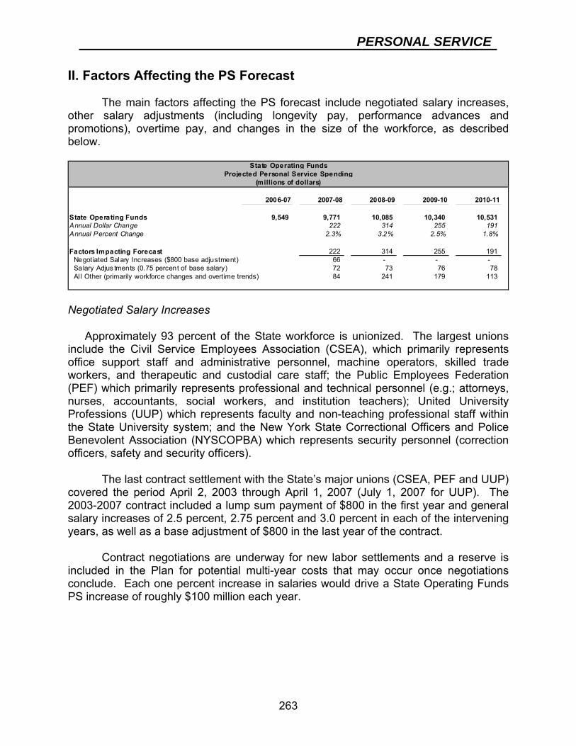
PERSONAL SERVICE
263
II. Factors Affecting the PS Forecast The main factors affecting the PS forecast include negotiated salary increases,
other salary adjustments (including longevity pay, performance advances and promotions), overtime pay, and changes in the size of the workforce, as described below.
2006-07 2007-08 2008-09 2009-10 2010-11
State Operating Funds 9,549 9,771 10,085 10,340 10,531 Annual Dollar Change 222 314 255 191 Annual Percent Change 2.3% 3.2% 2.5% 1.8%
Factors Impacting Forecast 222 314 255 191 Negotiated Salary Increases ($800 base adjustment) 66 - - - Salary Adjus tments (0.75 percent of base salary) 72 73 76 78 Al l Other (primarily workforce changes and overtime trends) 84 241 179 113
State Operating FundsProjected Personal Service Spending
(millions of dollars)
Negotiated Salary Increases
Approximately 93 percent of the State workforce is unionized. The largest unions include the Civil Service Employees Association (CSEA), which primarily represents office support staff and administrative personnel, machine operators, skilled trade workers, and therapeutic and custodial care staff; the Public Employees Federation (PEF) which primarily represents professional and technical personnel (e.g.; attorneys, nurses, accountants, social workers, and institution teachers); United University Professions (UUP) which represents faculty and non-teaching professional staff within the State University system; and the New York State Correctional Officers and Police Benevolent Association (NYSCOPBA) which represents security personnel (correction officers, safety and security officers).
The last contract settlement with the State’s major unions (CSEA, PEF and UUP) covered the period April 2, 2003 through April 1, 2007 (July 1, 2007 for UUP). The 2003-2007 contract included a lump sum payment of $800 in the first year and general salary increases of 2.5 percent, 2.75 percent and 3.0 percent in each of the intervening years, as well as a base adjustment of $800 in the last year of the contract.
Contract negotiations are underway for new labor settlements and a reserve is included in the Plan for potential multi-year costs that may occur once negotiations conclude. Each one percent increase in salaries would drive a State Operating Funds PS increase of roughly $100 million each year.
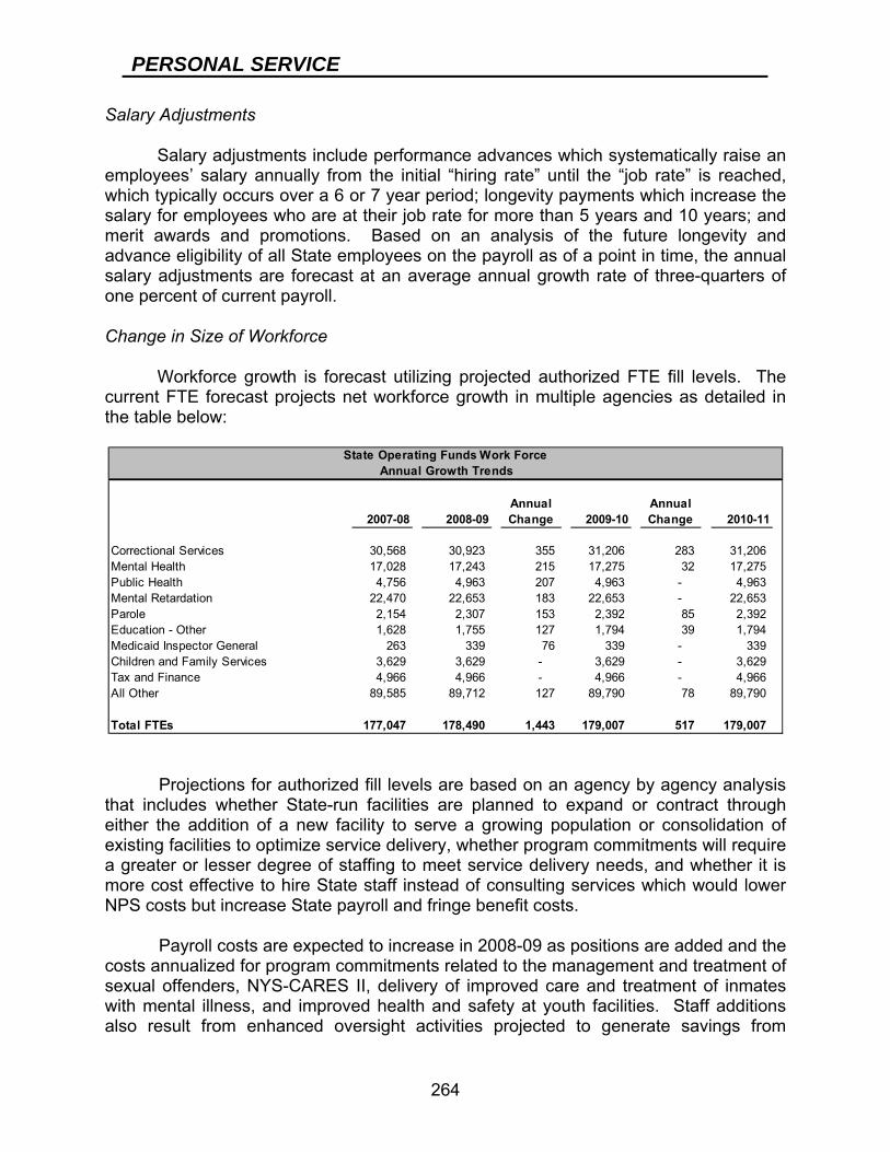
PERSONAL SERVICE
264
Salary Adjustments
Salary adjustments include performance advances which systematically raise an employees’ salary annually from the initial “hiring rate” until the “job rate” is reached, which typically occurs over a 6 or 7 year period; longevity payments which increase the salary for employees who are at their job rate for more than 5 years and 10 years; and merit awards and promotions. Based on an analysis of the future longevity and advance eligibility of all State employees on the payroll as of a point in time, the annual salary adjustments are forecast at an average annual growth rate of three-quarters of one percent of current payroll.
Change in Size of Workforce
Workforce growth is forecast utilizing projected authorized FTE fill levels. The current FTE forecast projects net workforce growth in multiple agencies as detailed in the table below:
Projections for authorized fill levels are based on an agency by agency analysis that includes whether State-run facilities are planned to expand or contract through either the addition of a new facility to serve a growing population or consolidation of existing facilities to optimize service delivery, whether program commitments will require a greater or lesser degree of staffing to meet service delivery needs, and whether it is more cost effective to hire State staff instead of consulting services which would lower NPS costs but increase State payroll and fringe benefit costs.
Payroll costs are expected to increase in 2008-09 as positions are added and the costs annualized for program commitments related to the management and treatment of sexual offenders, NYS-CARES II, delivery of improved care and treatment of inmates with mental illness, and improved health and safety at youth facilities. Staff additions also result from enhanced oversight activities projected to generate savings from
Annual Annual2007-08 2008-09 Change 2009-10 Change 2010-11
Correctional Services 30,568 30,923 355 31,206 283 31,206 Mental Health 17,028 17,243 215 17,275 32 17,275 Public Health 4,756 4,963 207 4,963 - 4,963 Mental Retardation 22,470 22,653 183 22,653 - 22,653 Parole 2,154 2,307 153 2,392 85 2,392 Education - Other 1,628 1,755 127 1,794 39 1,794 Medicaid Inspector General 263 339 76 339 - 339 Children and Family Services 3,629 3,629 - 3,629 - 3,629 Tax and Finance 4,966 4,966 - 4,966 - 4,966 All Other 89,585 89,712 127 89,790 78 89,790
Total FTEs 177,047 178,490 1,443 179,007 517 179,007
State Operating Funds Work ForceAnnual Growth Trends

PERSONAL SERVICE
265
increased Medicaid audit and fraud prevention and tax audit and compliance efforts. Other additions across numerous agencies, including Education and Public Health, reflect FTE increases commensurate with authorized fill levels.
The annual projected FTE increase of 2,973 in 2007-08, at an average cost of $55,000 per employee, results in an estimated annual increase in PS costs of roughly $163 million on a full year basis. Likewise, the expected annual FTE increases of 1,443 in 2008-09 and 517 in 2009-10 result in estimated higher PS costs of roughly $79 million and $28 million, respectively.
Overtime Costs
In addition, overtime costs are also taken into consideration based on prior agency specific experience. Overtime costs comprised roughly 5 percent of the State Operating Funds personal service spending in 2006-07. Approximately two-thirds of overtime costs were generated by the Department of Correctional Services and the Mental Hygiene agencies, as detailed in the table below.
2006-07Correctional Services 158 Mental Health 78 Mental Retardation 68 SUNY 44 State Police 43 Judiciary 34 All Other 59
Total Overtime 484 5 Year Average Annual Growth 10.3%
State Operating FundsOvertime
(millions of dollars)
Overview of the Workforce Cost Projection Tool (WCPT)
To support the analysis of the above factors that influence annual payroll projections, DOB uses an automated system, the Workforce Cost Projection Tool (WCPT). The WCPT projects future salary requirements for existing State employees for use by agency fiscal officers in the development of their Personal Service budget requests and by budget examiners in the development of their Personal Service budget recommendations.
The WCPT projects future salary costs for existing State employees from a payroll file that is produced by the Office of the State Comptroller’s (OSC’s) payroll
PERSONAL SERVICE
266
system. The projection methodology related to the various salary cost components is discussed in more detail below. Annual-Salaried Employee Salary Projections
The WCPT projects annual-salaried employee costs by calculating the future salaries of each annual-salaried employee listed in the base payroll and aggregating the results. The system does this by using the full time annual salary that appears in the base payroll file as its starting point, and adding planned salary increases, performance advances, longevity payments and lump-sum payments where applicable. The addition of salary increases, including performance advances and longevity payments, is dependent upon union contract provisions. “Additional” or “Other” Compensation
“Additional” or “other” compensation includes annual payments such as location pay, geographic differentials, and shift differentials, that are paid to employees in addition to their base salaries. Eligibility for various types of additional compensation depends upon a variety of factors including the bargaining unit to which the employee’s position is assigned, the employee’s work location, the employee’s designated work hours and the nature of the employee’s work responsibilities. “Episodic” and “Non-Annual” Salaried Employee Costs
DOB began projecting “episodic” and “non-annual” salaried employee costs through the WCPT in 2006 for the 2007-2008 fiscal year. Episodic earnings are those earnings, such as overtime and standby pay, that are not as predictable as other contract terms. These earnings are summarized into earnings categories, such as non-annual salaried employee costs, overtime and lump-sum payments, and then aggregated by agency, fund, account, program, bargaining unit and union over 26 pay periods. Adjustments for Changes in Workforce Composition
DOB methodologies for projecting outyear annual salaries, additional compensation, episodic earnings, and non-annual salaried employee costs assume that there will be no change in the composition of the State workforce, such as new hires, separations, promotions, transfers, or position reclassifications or reallocations. Therefore, for a given budget year, adjustments must be made to the WCPT’s projections for these changes as well as for suballocations to other agencies and planned increases to non-statutory salaries. These adjustments are typically made by agency fiscal officers and DOB examiners during budget development.
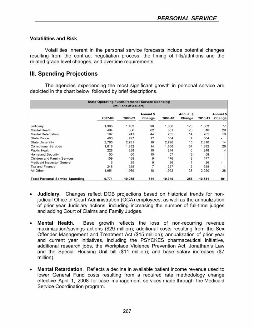
PERSONAL SERVICE
267
Volatilities and Risk
Volatilities inherent in the personal service forecasts include potential changes resulting from the contract negotiation process, the timing of fills/attritions and the related grade level changes, and overtime requirements.
III. Spending Projections The agencies experiencing the most significant growth in personal service are depicted in the chart below, followed by brief descriptions.
Annual $ Annual $ Annual $2007-08 2008-09 Change 2009-10 Change 2010-11 Change
Judiciary 1,365 1,463 98 1,586 123 1,663 77 Mental Health 494 556 62 581 25 610 29 Mental Retardation 197 241 44 255 14 265 10 State Police 480 497 17 504 7 504 - State University 2,765 2,781 16 2,796 15 2,810 14 Correctional Services 1,818 1,832 14 1,866 34 1,892 26 Public Health 228 238 10 244 6 248 4 Homeland Security 50 60 10 57 (3) 58 1 Children and Family Services 159 168 9 176 8 177 1 Medicaid Inspector General 16 25 9 26 1 26 - Tax and Finance 248 255 7 257 2 258 1 All Other 1,951 1,969 18 1,992 23 2,020 28
Total Personal Service Spending 9,771 10,085 314 10,340 255 10,531 191
State Operating Funds Personal Service Spending(millions of dollars)
• Judiciary. Changes reflect DOB projections based on historical trends for non-
judicial Office of Court Administration (OCA) employees, as well as the annualization of prior year Judiciary actions, including increasing the number of full-time judges and adding Court of Claims and Family Judges.
• Mental Health. Base growth reflects the loss of non-recurring revenue
maximization/savings actions ($29 million); additional costs resulting from the Sex Offender Management and Treatment Act ($15 million); annualization of prior year and current year initiatives, including the PSYCKES pharmaceutical initiative, additional research jobs, the Workplace Violence Prevention Act, Jonathan’s Law and the Special Housing Unit bill ($11 million); and base salary increases ($7 million).
• Mental Retardation. Reflects a decline in available patient income revenue used to
lower General Fund costs resulting from a required rate methodology change effective April 1, 2008 for case management services made through the Medicaid Service Coordination program.

PERSONAL SERVICE
268
• State Police. The spending growth is driven primarily by the State Police’s takeover of patrol costs on Interstate highway 84 in 2008-09 that were previously financed with proceeds from toll revenues that have been discontinued.
• State University. The total workforce for SUNY is approximately 40,000 positions
supported by State Operating Funds including tuition revenues and other non-General Fund revenue sources. The annual growth is driven largely by costs associated with contractual salary increases, multi-year initiatives and legislative additions.
• Correctional Services. Growth is primarily attributable to the Sex Offender
Management and Treatment Act and the restricted use of special housing units for mentally ill inmates that are expected to result in an increased need for correction officers, thus driving higher workforce levels.
• Public Health. Growth primarily reflects the annualization of 79 new positions
included in the 2007-08 Budget as well as anticipated cost increases associated with filling vacant positions.
• Homeland Security. Reflects personal service costs of National Guard response to
ongoing heightened alert status (Orange Alert). This response covers activities such as statewide infrastructure protection, New York City Orange Alert protection, airport security measures, northern border security, and security at the Empire State Plaza.
• Children and Family Services. Increases primarily reflect the expected loss of
non-recurring Federal revenue used to offset General Fund costs ($5 million) and the additional annualized cost of 218 new youth facility jobs added part way through 2007-08 ($4 million).
• Medicaid Inspector General. This newly created agency is expected to continue to
expand operations in 2008-09 in order to be able to fulfill the agency's goals. The agency expects PS costs to increase as currently vacant positions are filled.
• Tax and Finance. Changes reflect the annualization of roughly 200 additional full-
time employees added for enhanced audit activity and information technology purposes.
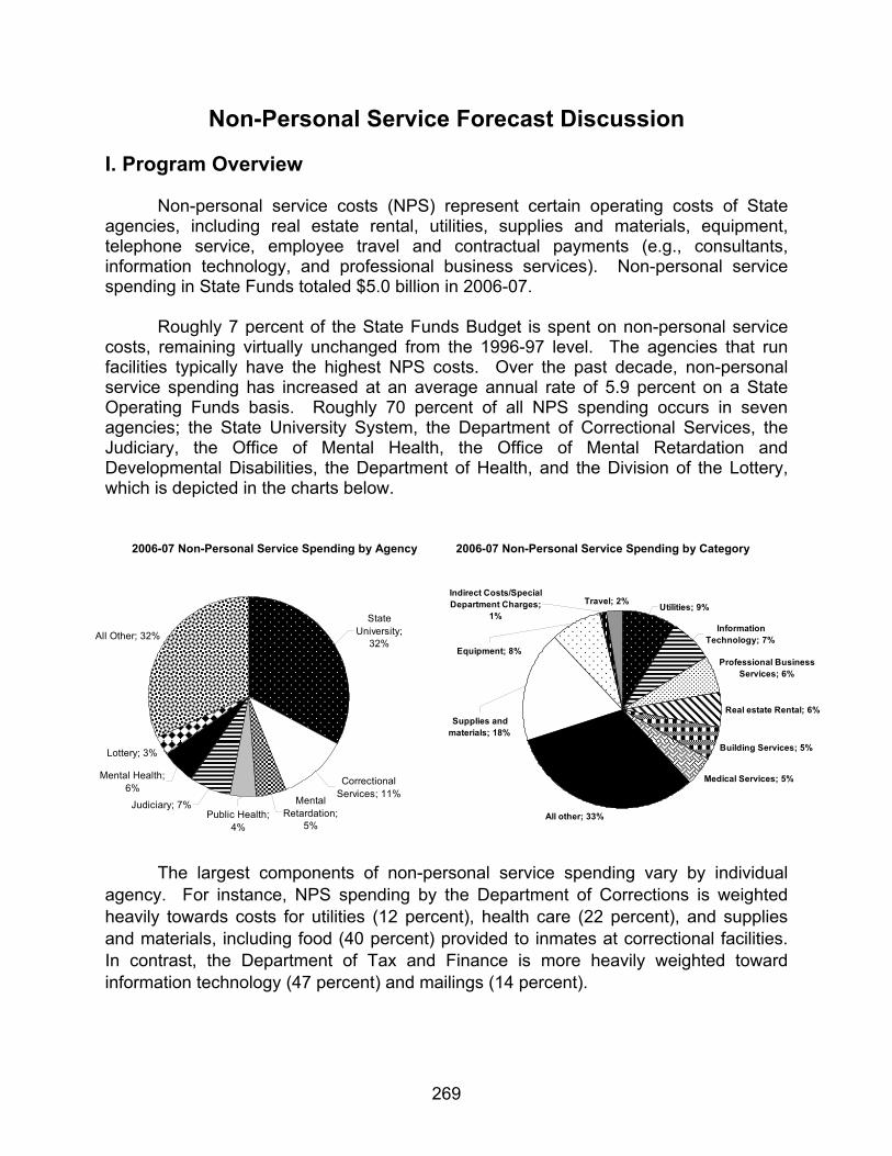
269
Non-Personal Service Forecast Discussion I. Program Overview
Non-personal service costs (NPS) represent certain operating costs of State
agencies, including real estate rental, utilities, supplies and materials, equipment, telephone service, employee travel and contractual payments (e.g., consultants, information technology, and professional business services). Non-personal service spending in State Funds totaled $5.0 billion in 2006-07.
Roughly 7 percent of the State Funds Budget is spent on non-personal service
costs, remaining virtually unchanged from the 1996-97 level. The agencies that run facilities typically have the highest NPS costs. Over the past decade, non-personal service spending has increased at an average annual rate of 5.9 percent on a State Operating Funds basis. Roughly 70 percent of all NPS spending occurs in seven agencies; the State University System, the Department of Correctional Services, the Judiciary, the Office of Mental Health, the Office of Mental Retardation and Developmental Disabilities, the Department of Health, and the Division of the Lottery, which is depicted in the charts below.
The largest components of non-personal service spending vary by individual agency. For instance, NPS spending by the Department of Corrections is weighted heavily towards costs for utilities (12 percent), health care (22 percent), and supplies and materials, including food (40 percent) provided to inmates at correctional facilities. In contrast, the Department of Tax and Finance is more heavily weighted toward information technology (47 percent) and mailings (14 percent).
Lottery; 3%
All Other; 32%
Mental Health; 6%
Judiciary; 7%Public Health;
4%
Mental Retardation;
5%
Correctional Services; 11%
State University;
32%
2006-07 Non-Personal Service Spending by Agency 2006-07 Non-Personal Service Spending by Category
Utilities; 9%
Information Technology; 7%
Professional Business Services; 6%
Real estate Rental; 6%
Building Services; 5%
Medical Services; 5%
All other; 33%
Travel; 2%
Equipment; 8%
Supplies and materials; 18%
Indirect Costs/Special Department Charges;
1%
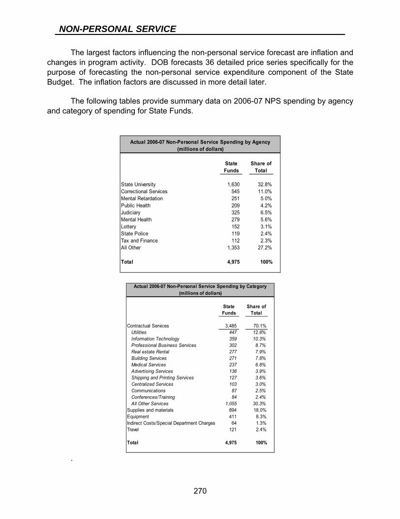
NON-PERSONAL SERVICE
270
State Funds
Share of Total
State University 1,630 32.8%Correctional Services 545 11.0%Mental Retardation 251 5.0%Public Health 209 4.2%Judiciary 325 6.5%Mental Health 279 5.6%Lottery 152 3.1%State Police 119 2.4%Tax and Finance 112 2.3%All Other 1,353 27.2%
Total 4,975 100%
Actual 2006-07 Non-Personal Service Spending by Agency(millions of dollars)
State Funds
Share of Total
Contractual Services 3,485 70.1%Utilities 447 12.8%Information Technology 359 10.3%Professional Business Services 302 8.7%Real estate Rental 277 7.9%Building Services 271 7.8%Medical Services 237 6.8%Advertising Services 136 3.9%Shipping and Printing Services 127 3.6%Centralized Services 103 3.0%Communications 87 2.5%Conferences/Training 84 2.4%All Other Services 1,055 30.3%
Supplies and materials 894 18.0%Equipment 411 8.3%Indirect Costs/Special Department Charges 64 1.3%Travel 121 2.4%
Total 4,975 100%
Actual 2006-07 Non-Personal Service Spending by Category(millions of dollars)
The largest factors influencing the non-personal service forecast are inflation and changes in program activity. DOB forecasts 36 detailed price series specifically for the purpose of forecasting the non-personal service expenditure component of the State Budget. The inflation factors are discussed in more detail later.
The following tables provide summary data on 2006-07 NPS spending by agency and category of spending for State Funds.
.
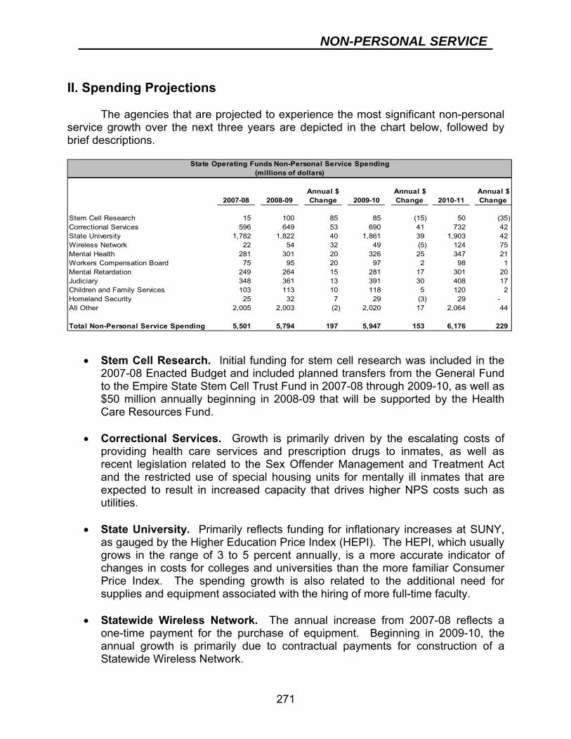
NON-PERSONAL SERVICE
271
II. Spending Projections
The agencies that are projected to experience the most significant non-personal
service growth over the next three years are depicted in the chart below, followed by brief descriptions.
Annual $ Annual $ Annual $2007-08 2008-09 Change 2009-10 Change 2010-11 Change
Stem Cell Research 15 100 85 85 (15) 50 (35) Correctional Services 596 649 53 690 41 732 42 State University 1,782 1,822 40 1,861 39 1,903 42 Wireless Network 22 54 32 49 (5) 124 75 Mental Health 281 301 20 326 25 347 21 Workers Compensation Board 75 95 20 97 2 98 1 Mental Retardation 249 264 15 281 17 301 20 Judiciary 348 361 13 391 30 408 17 Children and Family Services 103 113 10 118 5 120 2 Homeland Security 25 32 7 29 (3) 29 - All Other 2,005 2,003 (2) 2,020 17 2,064 44
Total Non-Personal Service Spending 5,501 5,794 197 5,947 153 6,176 229
State Operating Funds Non-Personal Service Spending(millions of dollars)
• Stem Cell Research. Initial funding for stem cell research was included in the 2007-08 Enacted Budget and included planned transfers from the General Fund to the Empire State Stem Cell Trust Fund in 2007-08 through 2009-10, as well as $50 million annually beginning in 2008-09 that will be supported by the Health Care Resources Fund.
• Correctional Services. Growth is primarily driven by the escalating costs of
providing health care services and prescription drugs to inmates, as well as recent legislation related to the Sex Offender Management and Treatment Act and the restricted use of special housing units for mentally ill inmates that are expected to result in increased capacity that drives higher NPS costs such as utilities.
• State University. Primarily reflects funding for inflationary increases at SUNY,
as gauged by the Higher Education Price Index (HEPI). The HEPI, which usually grows in the range of 3 to 5 percent annually, is a more accurate indicator of changes in costs for colleges and universities than the more familiar Consumer Price Index. The spending growth is also related to the additional need for supplies and equipment associated with the hiring of more full-time faculty.
• Statewide Wireless Network. The annual increase from 2007-08 reflects a
one-time payment for the purchase of equipment. Beginning in 2009-10, the annual growth is primarily due to contractual payments for construction of a Statewide Wireless Network.

NON-PERSONAL SERVICE
272
• Mental Health. Reflects overall inflationary increases, including assumed 4
percent increases for energy costs; roughly 10 percent for pharmacy costs that is primarily driven by increased costs for psychotropic drugs ($15 million), and a significant increase in utilization projected as people with mental illness are living longer and using more drugs as they age; and additional costs resulting from the Sex Offender Management and Treatment Act ($3 million).
• Worker’s Compensation Board. Funding increase to allow the continuation of benefit payments to injured workers covered by bankrupt self-insurance plans.
• Mental Retardation. Primarily reflects a 2.5 percent overall inflationary increase
($9 million), as well as a roughly 10 percent increase for pharmacy costs ($5 million) that is primarily driven by increased costs for certain drugs which tend to be more expensive and a significant projected increase in utilization consistent with increasing life expectancy.
• Judiciary. The increase is driven by inflation and increasing court security costs,
Law Guardian/Assigned Counsel costs and additional costs generated by each new judgeship. In 2009-10 new regulations regarding maximum caseload for Law Guardians, as well as increased State aid for improving town and village courts and the maturation of the civil confinement program for sexual offenders, all contribute to escalating NPS costs.
• Children and Family Services. Growth is driven by the loss of Federal
revenues supporting development costs of the child welfare computer system ($5 million), general inflation ($3 million) and projected Office for Technology rate increases for services provided to the agency ($1 million).
• Homeland Security. Primarily reflects costs driven by the Oneida Training
Center project, which will provide training of all State First Responders/Potential First Responders in the event of an emergency (e.g., a terrorist attack or natural disaster).
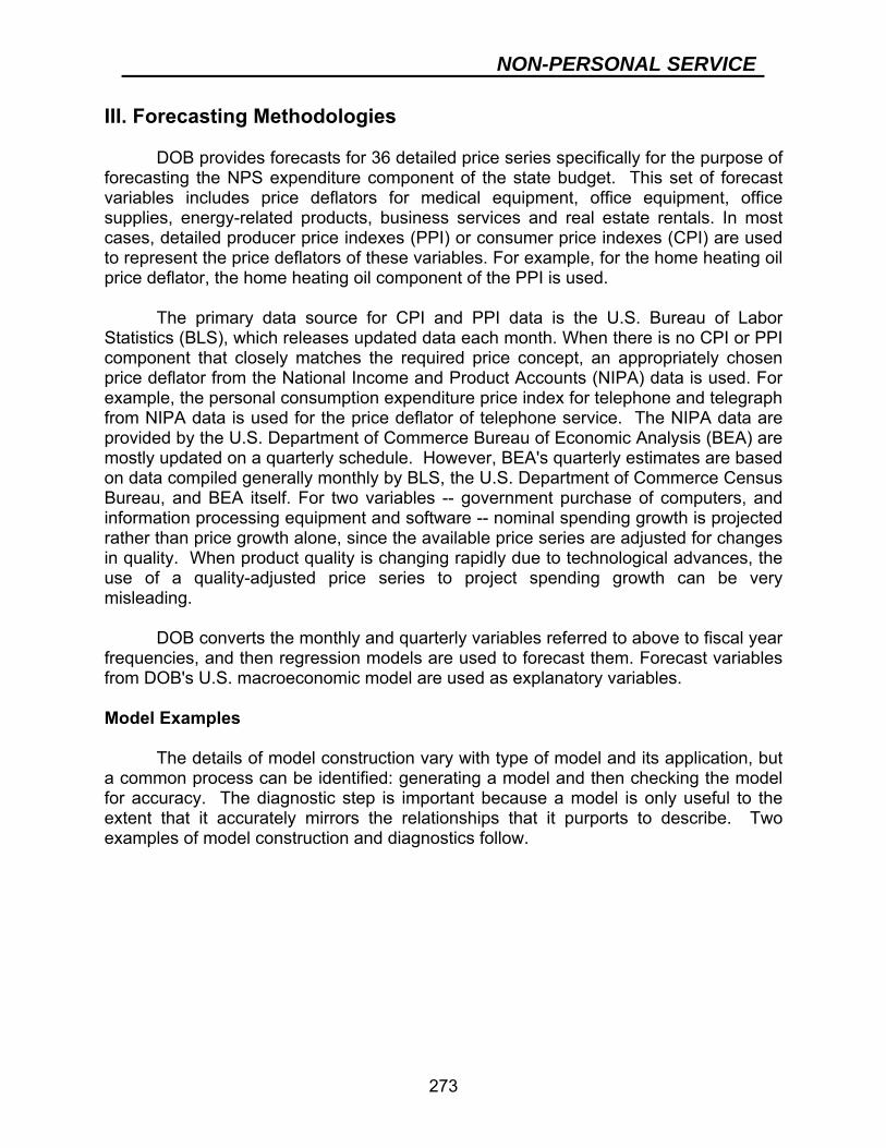
NON-PERSONAL SERVICE
273
III. Forecasting Methodologies
DOB provides forecasts for 36 detailed price series specifically for the purpose of forecasting the NPS expenditure component of the state budget. This set of forecast variables includes price deflators for medical equipment, office equipment, office supplies, energy-related products, business services and real estate rentals. In most cases, detailed producer price indexes (PPI) or consumer price indexes (CPI) are used to represent the price deflators of these variables. For example, for the home heating oil price deflator, the home heating oil component of the PPI is used.
The primary data source for CPI and PPI data is the U.S. Bureau of Labor
Statistics (BLS), which releases updated data each month. When there is no CPI or PPI component that closely matches the required price concept, an appropriately chosen price deflator from the National Income and Product Accounts (NIPA) data is used. For example, the personal consumption expenditure price index for telephone and telegraph from NIPA data is used for the price deflator of telephone service. The NIPA data are provided by the U.S. Department of Commerce Bureau of Economic Analysis (BEA) are mostly updated on a quarterly schedule. However, BEA's quarterly estimates are based on data compiled generally monthly by BLS, the U.S. Department of Commerce Census Bureau, and BEA itself. For two variables -- government purchase of computers, and information processing equipment and software -- nominal spending growth is projected rather than price growth alone, since the available price series are adjusted for changes in quality. When product quality is changing rapidly due to technological advances, the use of a quality-adjusted price series to project spending growth can be very misleading.
DOB converts the monthly and quarterly variables referred to above to fiscal year frequencies, and then regression models are used to forecast them. Forecast variables from DOB's U.S. macroeconomic model are used as explanatory variables. Model Examples
The details of model construction vary with type of model and its application, but a common process can be identified: generating a model and then checking the model for accuracy. The diagnostic step is important because a model is only useful to the extent that it accurately mirrors the relationships that it purports to describe. Two examples of model construction and diagnostics follow.
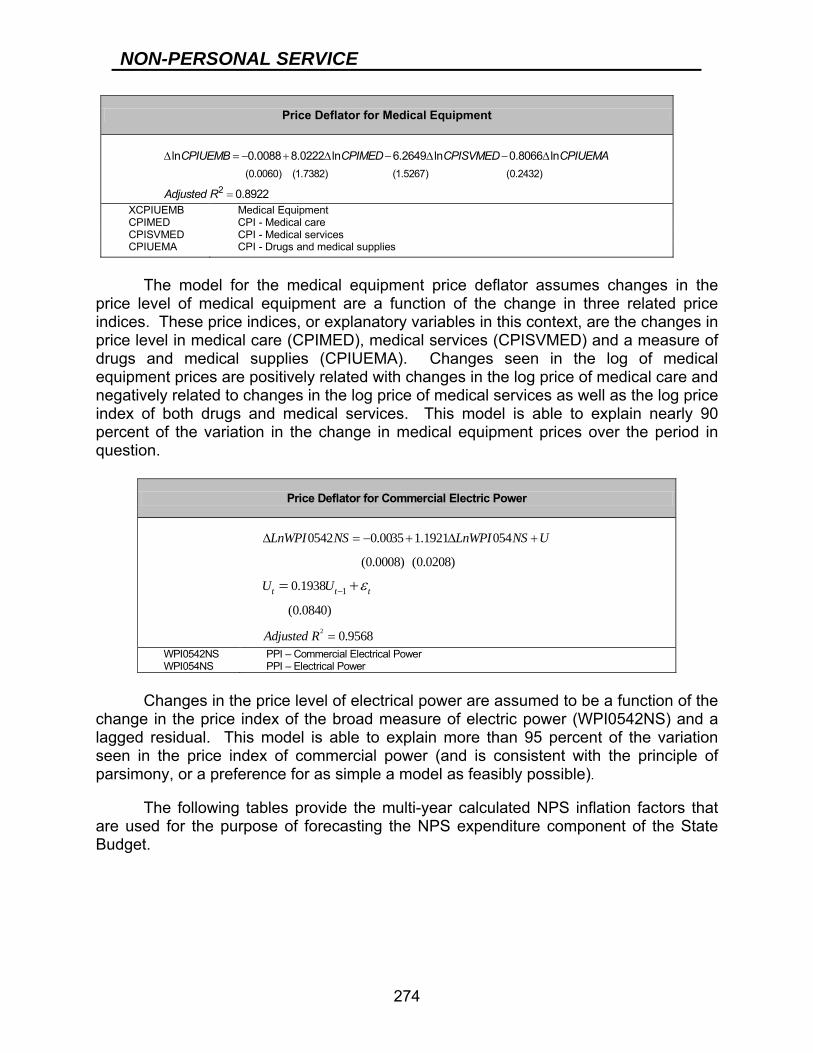
NON-PERSONAL SERVICE
274
Price Deflator for Medical Equipment
Δ = − + Δ − Δ − Δ
=2
(0.0060) (1.7382) (1.5267) (0.2432)
ln 0.0088 8.0222 ln 6.2649 ln 0.8066 ln
0.8922
CPIUEMB CPIMED CPISVMED CPIUEMA
Adjusted R
XCPIUEMB Medical Equipment CPIMED CPI - Medical care CPISVMED CPI - Medical services CPIUEMA CPI - Drugs and medical supplies
The model for the medical equipment price deflator assumes changes in the price level of medical equipment are a function of the change in three related price indices. These price indices, or explanatory variables in this context, are the changes in price level in medical care (CPIMED), medical services (CPISVMED) and a measure of drugs and medical supplies (CPIUEMA). Changes seen in the log of medical equipment prices are positively related with changes in the log price of medical care and negatively related to changes in the log price of medical services as well as the log price index of both drugs and medical services. This model is able to explain nearly 90 percent of the variation in the change in medical equipment prices over the period in question.
Changes in the price level of electrical power are assumed to be a function of the change in the price index of the broad measure of electric power (WPI0542NS) and a lagged residual. This model is able to explain more than 95 percent of the variation seen in the price index of commercial power (and is consistent with the principle of parsimony, or a preference for as simple a model as feasibly possible).
The following tables provide the multi-year calculated NPS inflation factors that
are used for the purpose of forecasting the NPS expenditure component of the State Budget.
Price Deflator for Commercial Electric Power
2
1
0542 0.0035 1.1921 054
(0.0008) (0.0208)
0.1938
(0.0840)
0.9568
t t t
LnWPI NS LnWPI NS U
U U
Adjusted R
ε−
Δ = − + Δ +
=
= +
WPI0542NS PPI – Commercial Electrical Power WPI054NS PPI – Electrical Power
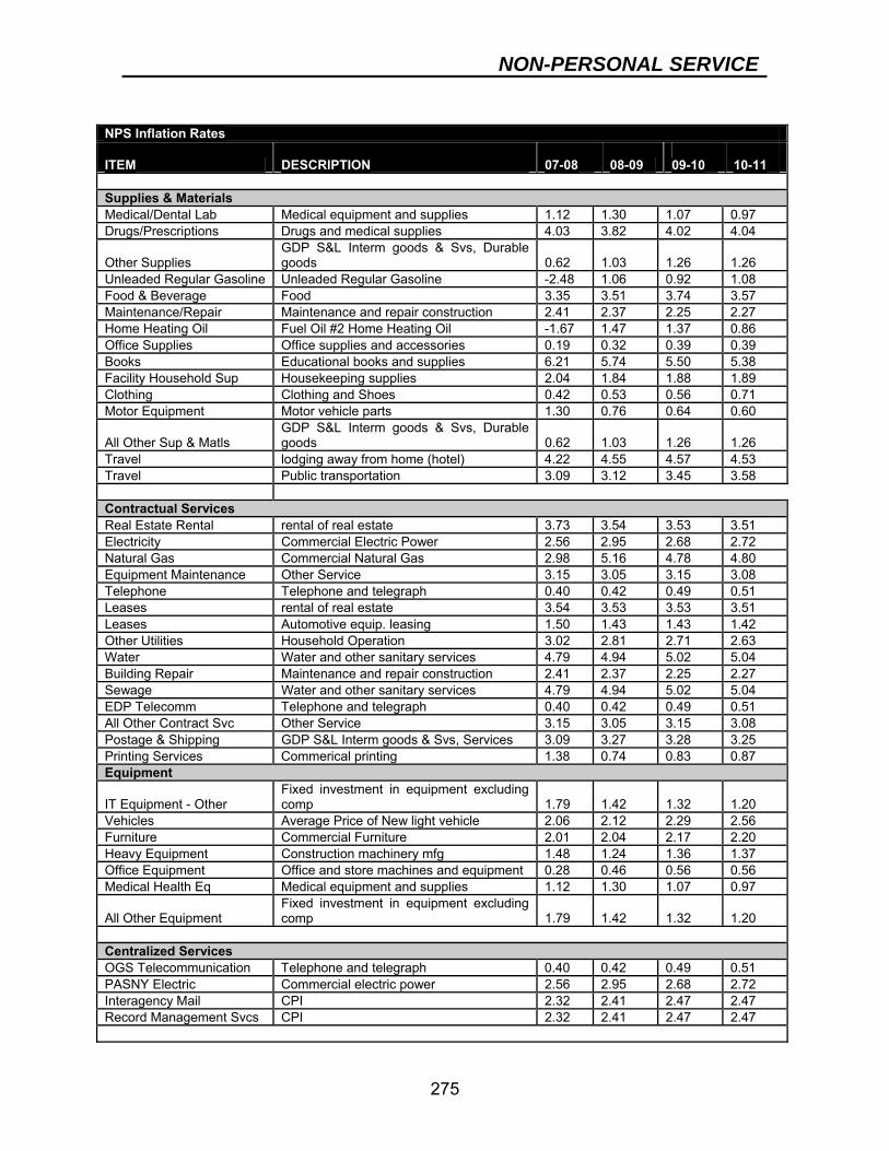
NON-PERSONAL SERVICE
275
NPS Inflation Rates
ITEM DESCRIPTION 07-08 08-09 09-10
10-11
Supplies & Materials Medical/Dental Lab Medical equipment and supplies 1.12 1.30 1.07 0.97 Drugs/Prescriptions Drugs and medical supplies 4.03 3.82 4.02 4.04
Other Supplies GDP S&L Interm goods & Svs, Durable goods 0.62 1.03 1.26 1.26
Unleaded Regular Gasoline Unleaded Regular Gasoline -2.48 1.06 0.92 1.08 Food & Beverage Food 3.35 3.51 3.74 3.57 Maintenance/Repair Maintenance and repair construction 2.41 2.37 2.25 2.27 Home Heating Oil Fuel Oil #2 Home Heating Oil -1.67 1.47 1.37 0.86 Office Supplies Office supplies and accessories 0.19 0.32 0.39 0.39 Books Educational books and supplies 6.21 5.74 5.50 5.38 Facility Household Sup Housekeeping supplies 2.04 1.84 1.88 1.89 Clothing Clothing and Shoes 0.42 0.53 0.56 0.71 Motor Equipment Motor vehicle parts 1.30 0.76 0.64 0.60
All Other Sup & Matls GDP S&L Interm goods & Svs, Durable goods 0.62 1.03 1.26 1.26
Travel lodging away from home (hotel) 4.22 4.55 4.57 4.53 Travel Public transportation 3.09 3.12 3.45 3.58 Contractual Services Real Estate Rental rental of real estate 3.73 3.54 3.53 3.51 Electricity Commercial Electric Power 2.56 2.95 2.68 2.72 Natural Gas Commercial Natural Gas 2.98 5.16 4.78 4.80 Equipment Maintenance Other Service 3.15 3.05 3.15 3.08 Telephone Telephone and telegraph 0.40 0.42 0.49 0.51 Leases rental of real estate 3.54 3.53 3.53 3.51 Leases Automotive equip. leasing 1.50 1.43 1.43 1.42 Other Utilities Household Operation 3.02 2.81 2.71 2.63 Water Water and other sanitary services 4.79 4.94 5.02 5.04 Building Repair Maintenance and repair construction 2.41 2.37 2.25 2.27 Sewage Water and other sanitary services 4.79 4.94 5.02 5.04 EDP Telecomm Telephone and telegraph 0.40 0.42 0.49 0.51 All Other Contract Svc Other Service 3.15 3.05 3.15 3.08 Postage & Shipping GDP S&L Interm goods & Svs, Services 3.09 3.27 3.28 3.25 Printing Services Commerical printing 1.38 0.74 0.83 0.87 Equipment
IT Equipment - Other Fixed investment in equipment excluding comp 1.79 1.42 1.32 1.20
Vehicles Average Price of New light vehicle 2.06 2.12 2.29 2.56 Furniture Commercial Furniture 2.01 2.04 2.17 2.20 Heavy Equipment Construction machinery mfg 1.48 1.24 1.36 1.37 Office Equipment Office and store machines and equipment 0.28 0.46 0.56 0.56 Medical Health Eq Medical equipment and supplies 1.12 1.30 1.07 0.97
All Other Equipment Fixed investment in equipment excluding comp 1.79 1.42 1.32 1.20
Centralized Services OGS Telecommunication Telephone and telegraph 0.40 0.42 0.49 0.51 PASNY Electric Commercial electric power 2.56 2.95 2.68 2.72 Interagency Mail CPI 2.32 2.41 2.47 2.47 Record Management Svcs CPI 2.32 2.41 2.47 2.47
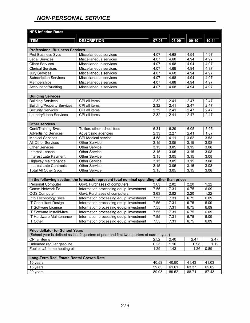
NON-PERSONAL SERVICE
276
NPS Inflation Rates
ITEM DESCRIPTION 07-08 08-09 09-10
10-11
Professional Business Services Prof Business Svcs Miscellaneous services 4.07 4.68 4.94 4.97 Legal Services Miscellaneous services 4.07 4.68 4.94 4.97 Client Services Miscellaneous services 4.07 4.68 4.94 4.97 Clerical Services Miscellaneous services 4.07 4.68 4.94 4.97 Jury Services Miscellaneous services 4.07 4.68 4.94 4.97 Subscription Services Miscellaneous services 4.07 4.68 4.94 4.97 Memberships Miscellaneous services 4.07 4.68 4.94 4.97 Accounting/Auditing Miscellaneous services 4.07 4.68 4.94 4.97 Building Services Building Services CPI all items 2.32 2.41 2.47 2.47 Building/Property Services CPI all items 2.32 2.41 2.47 2.47 Security Services CPI all items 2.32 2.41 2.47 2.47 Laundry/Linen Services CPI all items 2.32 2.41 2.47 2.47 Other services Conf/Training Svcs Tuition, other school fees 6.31 6.29 6.05 5.95 Advertising Services Advertising agencies 2.33 2.27 2.41 1.87 Medical Services CPI Medical service 4.58 4.11 3.62 3.53 All Other Services Other Service 3.15 3.05 3.15 3.08 Other Services Other Service 3.15 3.05 3.15 3.08 Interest Leases Other Service 3.15 3.05 3.15 3.08 Interest Late Payment Other Service 3.15 3.05 3.15 3.08 Highway Maintenance Other Service 3.15 3.05 3.15 3.08 Interest Late Contracts Other Service 3.15 3.05 3.15 3.08 Total All Other Svcs Other Service 3.15 3.05 3.15 3.08 In the following section, the forecasts represent total nominal spending rather than prices Personal Computer Govt. Purchases of computers 3.63 2.82 2.20 1.22 Comm Network Eq Information processing equip. investment 7.55 7.31 6.75 6.09 OGS Computer Govt. Purchases of computers 3.63 2.82 2.20 1.22 Info Technology Svcs Information processing equip. investment 7.55 7.31 6.75 6.09 IT Consultant Design Information processing equip. investment 7.55 7.31 6.75 6.09 IT Software License Information processing equip. investment 7.55 7.31 6.75 6.09 IT Software Install/Mtce Information processing equip. investment 7.55 7.31 6.75 6.09 IT Hardware Maintenance Information processing equip. investment 7.55 7.31 6.75 6.09 IT Other Information processing equip. investment 7.55 7.31 6.75 6.09 Price deflator for School Years (School year is defined as last 2 quarters of prior and first two quarters of current year) CPI all items 2.52 2.40 2.47 2.47 Unleaded regular gasoline 0.23 1.10 0.98 1.12 Fuel oil #2 home heating oil 1.29 1.43 1.26 0.89 Long-Term Real Estate Rental Growth Rate 10 years 40.58 40.90 41.43 41.03 15 years 59.83 61.61 63.37 65.02 20 years 89.93 89.52 88.71 87.43
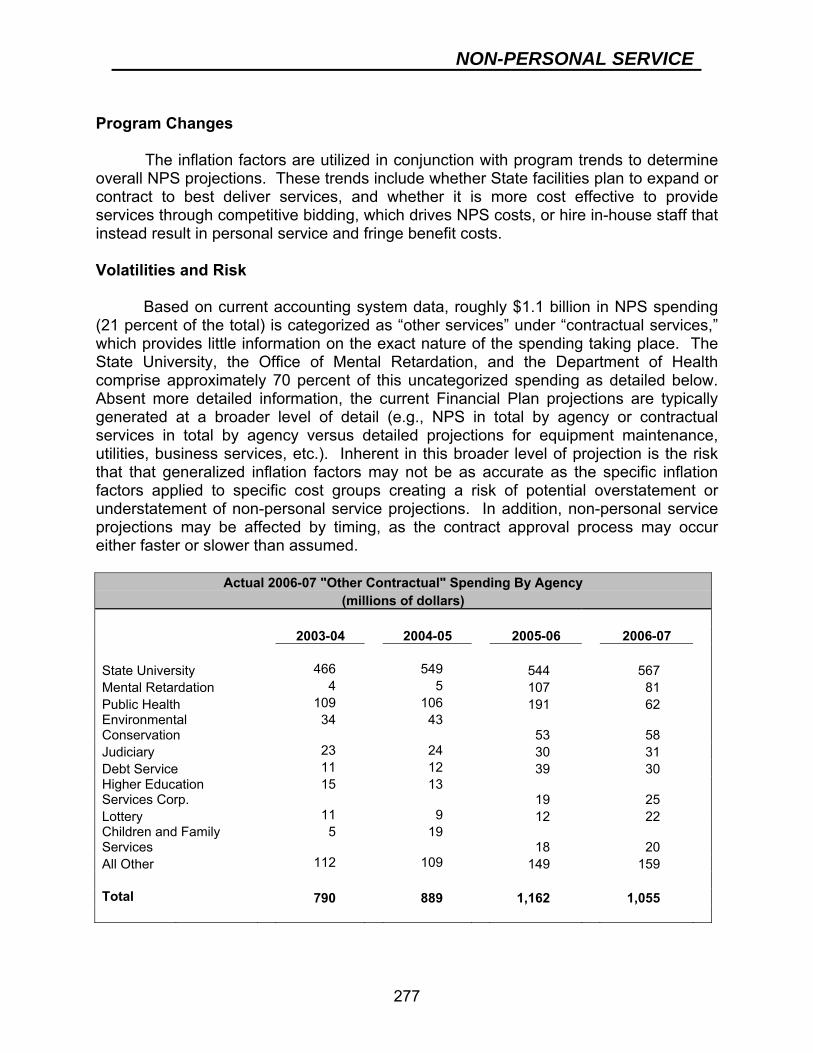
NON-PERSONAL SERVICE
277
Program Changes
The inflation factors are utilized in conjunction with program trends to determine overall NPS projections. These trends include whether State facilities plan to expand or contract to best deliver services, and whether it is more cost effective to provide services through competitive bidding, which drives NPS costs, or hire in-house staff that instead result in personal service and fringe benefit costs.
Volatilities and Risk
Based on current accounting system data, roughly $1.1 billion in NPS spending (21 percent of the total) is categorized as “other services” under “contractual services,” which provides little information on the exact nature of the spending taking place. The State University, the Office of Mental Retardation, and the Department of Health comprise approximately 70 percent of this uncategorized spending as detailed below. Absent more detailed information, the current Financial Plan projections are typically generated at a broader level of detail (e.g., NPS in total by agency or contractual services in total by agency versus detailed projections for equipment maintenance, utilities, business services, etc.). Inherent in this broader level of projection is the risk that that generalized inflation factors may not be as accurate as the specific inflation factors applied to specific cost groups creating a risk of potential overstatement or understatement of non-personal service projections. In addition, non-personal service projections may be affected by timing, as the contract approval process may occur either faster or slower than assumed.
Actual 2006-07 "Other Contractual" Spending By Agency (millions of dollars)
2003-04 2004-05 2005-06 2006-07 State University 466 549 544 567 Mental Retardation 4 5 107 81 Public Health 109 106 191 62 Environmental Conservation
34 43 53 58
Judiciary 23 24 30 31 Debt Service 11 12 39 30 Higher Education Services Corp.
15 13 19 25
Lottery 11 9 12 22 Children and Family Services
5 19 18 20
All Other 112 109 149 159 Total 790 889 1,162 1,055

278
Employee Health Insurance I. Program Overview
Background
Approximately 650,000 employees, retirees and their dependents are enrolled in the State's health insurance program. The number increases to over a million people if local government enrollees are included.
The State's share of health insurance premiums for employees and current retirees is 90 percent for individual coverage and 75 percent for dependent coverage. Employees and retirees contribute 10 percent and 25 percent for individual coverage and dependent coverage, respectively. However, the weighted average or "blended" contribution shares for the Empire Plan for both individual and dependent coverage result in an 86 percent employer share and 14 percent employee/retiree share -- after including all retirees and factoring in the value of the sick leave credit, where a retiree can use his/her unused sick leave credits to pay for part or all of his/her share of the health insurance premium. For retirees only, the employer share grows to more than 91 percent due to the sick leave credit described above and the fact that for pre-1982 retirees the State taxpayers pay 100 percent of the health insurance premium cost for individual coverage and 75 percent for dependent coverage.
The total 2007 annual cost of health insurance is $5,876 for individual coverage and $13,177 for family coverage. For the 2007-08 fiscal year the State is expected to spend an estimated $2.6 billion for employee/retiree health insurance (including the health insurance costs of the Legislature and the Judiciary.)
Spending Trend
Since 1995, the State's cost of employee health insurance has grown dramatically, more than doubling in a ten year period with an average of nine percent year-to-year growth over the past five years. These cost increases are attributed primarily to:
• the increased cost of health care generally, including prescription drugs;
• the extent of utilization by employees, retirees and dependents; and • the type and level of benefits provided under the State’s health
insurance plan, which for the most part are determined in collective bargaining with the State’s employee unions.
EMPLOYEE HEALTH INSURANCE
279
Current Challenges
The State is now actively negotiating with its employee unions on health insurance and other benefits, as well as compensation. The outcome of those negotiations will significantly shape the health insurance program and its costs and savings measures for the duration of the agreements.
A second major challenge involves implementation of a new accounting rule promulgated by the Governmental Accounting Standards Board (GASB). “GASB 45” requires the State and other public employers to report their post-employment health insurance liabilities for current employees and retirees starting in 2008. An actuarial analysis completed by Buck Consultants earlier this year concluded that the State's estimated liability is approximately $49.7 billion.
Although GASB 45 requires public employers to report their post-employment health insurance liabilities, it does not require pre-funding of those benefits. The State Health Insurance Council, consisting of the Director of Employee Relations, the President of the Civil Service Commission, and DOB, is continuing to evaluate long-term funding strategies for this liability.
II. Key Forecasting Data and Assumptions
The first step in forecasting employee health insurance costs for the Executive Budget begins in late Summer/early Fall with the establishment of Health Insurance premium rates for the coming year. The Department of Civil Service, in consultation with the Governor's Office of Employee Relations and DOB, negotiates the premium rates with the various health insurance carriers. Negotiations are based on a review of current experience and trends, leading to a projection of increases in such factors as utilization, the cost of claims, administrative costs and the impact of regulatory costs. When negotiations with the carriers are complete, the rates are sent to DOB for final approval. New premiums typically take effect at the beginning of the calendar year.
Data on current and projected enrollments (employee and retiree) are provided by the Department of Civil Service, as the ongoing administrator of the Plan.
A third factor in projecting the costs is the impact of any scheduled changes to benefit provisions that are generated from collective bargaining.
EMPLOYEE HEALTH INSURANCE
280
III. Spending Projections
Once the premium rates are approved, the employee health insurance costs for the new fiscal year can be estimated. The State’s health insurance premium cost is calculated by multiplying the enrollment figures for active State employees and retirees, by the respective new premium rates for individual and family coverage. The active State employee enrollment accounts for both the current workforce and any expected growth in the workforce. The retiree enrollment is based on current enrollment, adjusted for mortality rates and expected growth in the retiree population.
The total premium is then added to the Medicare Part B premium paid by the State on behalf of retirees. The State reimburses retirees for their Medicare B premiums because Medicare becomes the first payer for retirees’ medical costs, thereby reducing the State's costs. The costs of the State payment obligations under the sick leave credit program and the productivity enhancement program are added to the other components to generate the State's Employee Health Insurance estimate for the upcoming fiscal year. The sick leave credit and productivity enhancement programs allow retirees and active employees, respectively, to trade their sick leave days for reduced health insurance premiums, with the difference paid by the State.
The outyear forecasts are based on expected health insurance cost trends, utilization, and any expected enrollment changes that would result from anticipated fluctuations in the size of the State workforce. Every three of four years there may be additional increases or decreases to account for changes resulting from collective bargaining. The State and employee unions often agree upon changes to the design of the health insurance benefit that result in cost increases/decreases.
Employee Health Insurance Estimates (billions of dollars)
2006-07 2007-08 % 2008-09 % 2009-10 % 2010-11 %
Total $2.43 $2.56 5.5% $2.77 8.1% $3.01 8.7% $3.28 8.8%
Active Employees $1.52 $1.57 3.6% $1.70 8.1% $1.85 8.7% $2.01 8.7%
Retirees $0.91 $0.99 8.6% $1.07 7.9% $1.17 8.9% $1.27 9.0%
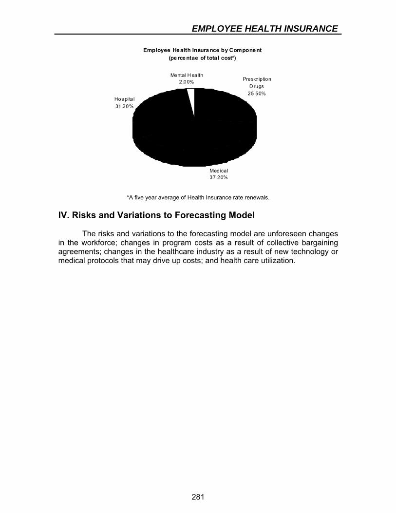
EMPLOYEE HEALTH INSURANCE
281
*A five year average of Health Insurance rate renewals. IV. Risks and Variations to Forecasting Model
The risks and variations to the forecasting model are unforeseen changes in the workforce; changes in program costs as a result of collective bargaining agreements; changes in the healthcare industry as a result of new technology or medical protocols that may drive up costs; and health care utilization.
Employee Health Insurance by Component(percentae of tota l cost*)
Pres cr iption D rugs
25.50%
Medical37.20%
Hos pi tal31.20%
Mental H ealth2.00%
282
Pensions I. Program Overview
Most State employees are members of the New York State and Local Retirement System, which consists of the Employees’ Retirement System (ERS) and the Police and Fire Retirement System (PFRS). Depending on the System and the benefit “tier” to which an individual employee belongs, employee contributions may or may not be required. In all cases, however, the State as employer must make annual payments to the System to fund the pension benefits that are promised to State employees. These pension benefits are protected by the State Constitution from any diminution. Although most State employees are members of ERS or PFRS, certain employees of the State University of New York and the State Education Department are enrolled in one of two other retirement systems: the New York State Teachers’ Retirement System (TRS) or the Optional Retirement Program (ORP). Unless specifically stated, the process and dollar amounts stated in this document apply only to State employees enrolled in ERS and PFRS.
The State's payments (as well as payments by local government employers for their employees, and employee contributions) go into the Common Retirement Fund (CRF), which, as of March 31, 2007, was valued at approximately $155 billion. The CRF holds the assets of both ERS, the system for civilian State and local government employees, and PFRS, the system for State and local government police officers and firefighters. The State Comptroller is the sole trustee of both of these systems.
In the late 1990's, the need for the State's annual pension payment was obviated by the extraordinary market returns of the Common Retirement Fund. Conversely, the stock market decline at the beginning of the current decade caused a dramatic increase in the State's annual pension payment. Significant benefit enhancements (including the elimination of the required three percent employee contribution by Tier 3 and Tier 4 employees after ten years of service and the implementation of cost of living adjustments) which were approved in 2000 also contributed to such increases.
II. Key Forecasting Data and Assumptions
Pension estimates result from the interplay of the two factors that determine the State's pension contribution, namely:
• The employer contribution rates determined by the Office of the State Comptroller (OSC), which are based on factors such as life expectancies, estimates of when employees typically retire, and the performance of the Common Retirement Fund, which holds the assets of the New York State and Local Retirement System. Employer contribution rates are set at the higher of an actuarially-determined rate based on the above factors, or a minimum contribution rate of 4.5 percent as prescribed by law.

PENSIONS
283
• Estimates of the State's salary base. These estimates begin with the current salary base and factor in known trends and planned changes, such as contractual salary increases resulting from collective bargaining and staffing changes associated with statutory or other mandates.
The employer contribution rates set by OSC are multiplied by the State's
salary base to determine the State's annual pension contribution. This calculation is adjusted for other pension costs such as administrative costs, prior year reconciliations, any unique amortization costs and the Group Life Insurance Program.
Calculating the pension cost estimate begins in earnest when OSC releases the employer contribution rates for the upcoming fiscal year, typically in early September. At this point, the rates are multiplied by DOB estimates of the State salary base to project the budget year pension payment. This amount is later refined when the State receives the "October Estimate" from OSC. This estimate, which OSC is statutorily required to provide, gives an in-depth analysis of the State's pension payment for the budget year and breaks down the various components of the payment, including normal costs, administrative costs, charges stemming from amortization of the State’s 2004-05 and 2005-06 obligations, reconciliation charges, group life insurance charges, and other charges associated with enacted legislation. OSC is also statutorily required to provide an updated budget year estimate in December and February, although these estimates are usually unchanged from the October Estimate.
Although outyear pension payments are ultimately dictated by the Retirement System, DOB staff work to anticipate changes by regularly monitoring the State's salary base and tracking the performance of the Common Retirement Fund. Tracking and forecasting the State's salary base is done by using information both from OSC and DOB and by keeping in mind any anticipated changes to the State's salary base, such as raises negotiated through the collective bargaining process or planned changes in the size of the State workforce. The Common Retirement Fund's annual performance is usually announced by OSC sometime after the end of each fiscal year.
Another factor that affects employer pension contribution rates is the use of the accounting technique known as smoothing. Used to reduce the year-to-year fluctuations in employer contribution rates from volatile investment returns, this process measures assets by averaging the gains and losses of equity investments over a five-year period. The smoothing process used by the Retirement System recognizes equity investment gains and losses at the rate of 20 percent per year for five years. As a result, the market performance in prior years can also affect employer contribution rates for an upcoming fiscal year.
A preliminary indication of outyear contribution rates is provided in the Comptroller’s Comprehensive Annual Financial Report (CAFR), but those rates are not intended to be hard estimates. The latest outyear projections by the Comptroller are contained in the CAFR for State fiscal year 2006-07, released on October 9, 2007. As shown below, these projections show that the ERS
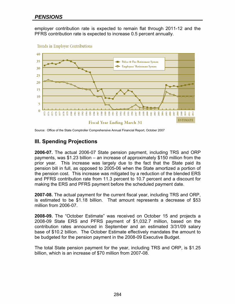
PENSIONS
284
employer contribution rate is expected to remain flat through 2011-12 and the PFRS contribution rate is expected to increase 0.5 percent annually.
Source: Office of the State Comptroller Comprehensive Annual Financial Report, October 2007
III. Spending Projections 2006-07. The actual 2006-07 State pension payment, including TRS and ORP payments, was $1.23 billion – an increase of approximately $150 million from the prior year. This increase was largely due to the fact that the State paid its pension bill in full, as opposed to 2005-06 when the State amortized a portion of the pension cost. This increase was mitigated by a reduction of the blended ERS and PFRS contribution rate from 11.3 percent to 10.7 percent and a discount for making the ERS and PFRS payment before the scheduled payment date. 2007-08. The actual payment for the current fiscal year, including TRS and ORP, is estimated to be $1.18 billion. That amount represents a decrease of $53 million from 2006-07. 2008-09. The “October Estimate” was received on October 15 and projects a 2008-09 State ERS and PFRS payment of $1,032.7 million, based on the contribution rates announced in September and an estimated 3/31/09 salary base of $10.2 billion. The October Estimate effectively mandates the amount to be budgeted for the pension payment in the 2008-09 Executive Budget. The total State pension payment for the year, including TRS and ORP, is $1.25 billion, which is an increase of $70 million from 2007-08.
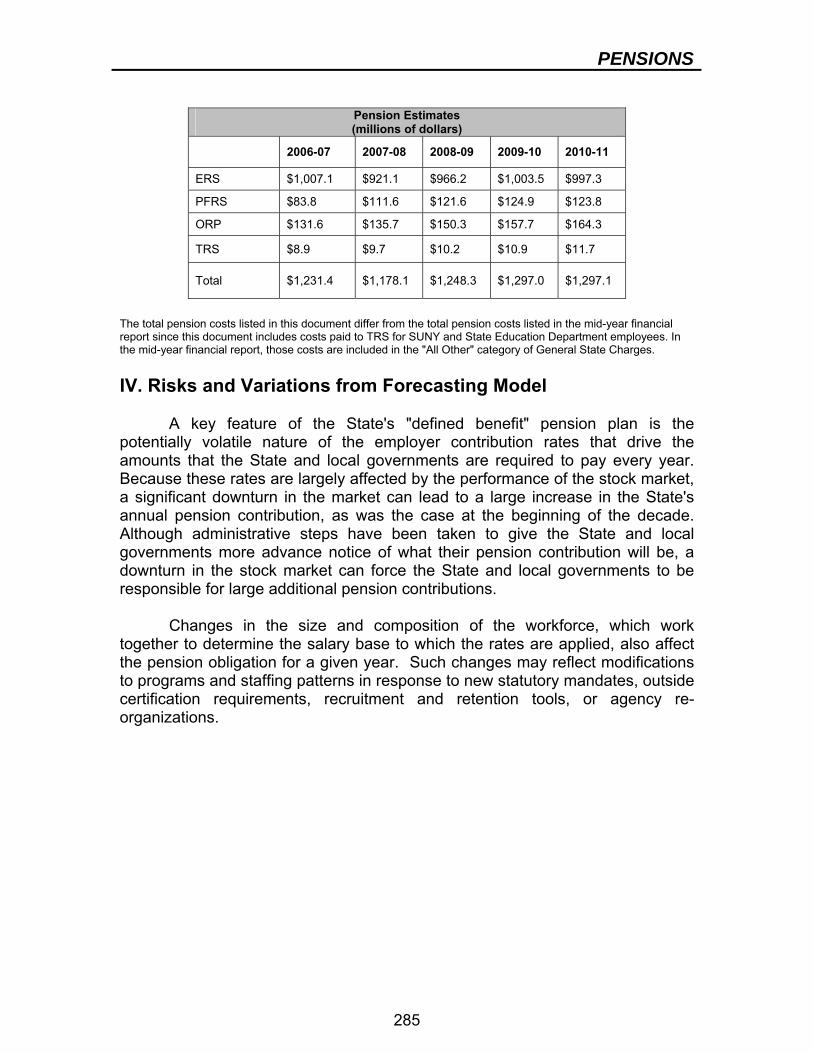
PENSIONS
285
Pension Estimates (millions of dollars)
2006-07 2007-08 2008-09 2009-10 2010-11
ERS $1,007.1 $921.1 $966.2 $1,003.5 $997.3
PFRS $83.8 $111.6 $121.6 $124.9 $123.8
ORP $131.6 $135.7 $150.3 $157.7 $164.3
TRS $8.9 $9.7 $10.2 $10.9 $11.7
Total $1,231.4 $1,178.1 $1,248.3 $1,297.0 $1,297.1
The total pension costs listed in this document differ from the total pension costs listed in the mid-year financial report since this document includes costs paid to TRS for SUNY and State Education Department employees. In the mid-year financial report, those costs are included in the "All Other" category of General State Charges. IV. Risks and Variations from Forecasting Model
A key feature of the State's "defined benefit" pension plan is the potentially volatile nature of the employer contribution rates that drive the amounts that the State and local governments are required to pay every year. Because these rates are largely affected by the performance of the stock market, a significant downturn in the market can lead to a large increase in the State's annual pension contribution, as was the case at the beginning of the decade. Although administrative steps have been taken to give the State and local governments more advance notice of what their pension contribution will be, a downturn in the stock market can force the State and local governments to be responsible for large additional pension contributions.
Changes in the size and composition of the workforce, which work together to determine the salary base to which the rates are applied, also affect the pension obligation for a given year. Such changes may reflect modifications to programs and staffing patterns in response to new statutory mandates, outside certification requirements, recruitment and retention tools, or agency re-organizations.


