Patrizia

NON DESTRUCTIVE TESTING

Ultrasonic Correlation Spectroscopy: new techniques forthe Nondestructive Evaluation of strongly scattering media

J. H. Pagea, M. L. Cowana and D. A. Weitzb

aDepartment of Physics and Astronomy, University of Manitoba, Winnipeg, MB R3T 2N2, CanadabDepartment of Physics and DEAS, Harvard University, Cambridge, MA 02138

Two new techniques in ultrasonic correlation spectroscopy, Dynamic Sound Scattering and Diffusing Acoustic WaveSpectroscopy, are described. Their potential for characterizing the dynamics of strongly scattering materials is illustrated withexperimental data on the motion of particles in fluidized beds.

Recent progress in understanding the propagationof acoustic waves in strongly scattering materials [1,2]has facilitated the development of two new techniquesin ultrasonic correlation spectroscopy [3]: DynamicSound Scattering (DSS) and Diffusing Acoustic WaveSpectroscopy (DAWS). These techniques providesensitive and complementary probes of the dynamicsof such systems, where direct imaging of theindividual scatterers (e.g. particles or inclusions) maybecome impossible due to the dominance of acousticspeckle. Rather than regarding speckle as adeleterious effect, these techniques exploit theexistence of speckle to obtain information on thescatterer dynamics, by measuring and analysing thetemporal fluctuations that occur in a speckle patternwhenever the scatterers are moving. Using correlationspectroscopy, the motion of the scatterers can bemeasured even when the variance exceeds the meanvelocity of the scatterers, yielding a wide range ofdynamic information that has not previously beenobtained in ultrasonic scattering experiments. In thispaper, we outline the basic principles behind DSS andDAWS, illustrating their potential as nondestructiveevaluation techniques with experimental results on thedynamics of fluidized beds.

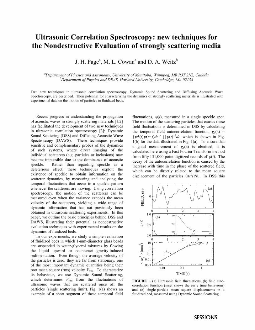
In our experiments, we study a simple realizationof fluidized beds in which 1-mm-diameter glass beadsare suspended in water-glycerol mixtures by flowingthe liquid upward to counteract gravity-inducedsedimentation. Even though the average velocity ofthe particles is zero, they are far from stationary, oneof the most important dynamic quantities being theirroot mean square (rms) velocity Vrms. To characterizeits behaviour, we use Dynamic Sound Scattering,which determines Vrms from the fluctuations ofultrasonic waves that are scattered once off theparticles (single scattering limit). Fig. 1(a) shows anexample of a short segment of these temporal field

fluctuations, ψ(t), measured in a single speckle spot.The motion of the scattering particles that causes thesefield fluctuations is determined in DSS by calculatingthe temporal field autocorrelation function, g1(τ) =fψ*(t)ψ(t+τ)dt / fGψ(t)G2dt, which is shown in Fig.1(b) for the data illustrated in Fig. 1(a). To ensure thata good measurement of g1(τ) is obtained, it iscalculated here using a Fast Fourier Transform methodfrom fifty 131,000-point digitized records of ψ(t). Thedecay of the autocorrelation function is caused by theincrease with time in the phase of the scattered field,which can be directly related to the mean squaredisplacement of the particles H∆r2(τ)I. In DSS this

0.01 0.1 11E-3

0.010.1

110

(c)

τ 2

< ∆r

y2 > (m

m2 )

TIME (s)

0 1 2 3 40.0

0.5

1.0(b)

g 1(τ)

0 1 2 3 4

0

(a)

FIEL

D, ψ

(τ)

0.0 0.2 0.40.0

0.5

1.0

FIGURE 1. (a) Ultrasonic field fluctuations, (b) field auto-correlation function (inset shows the early time behaviour)and (c) single-particle mean square displacements in afluidized bed, measured using Dynamic Sound Scattering.

relationship gives g1(τ) = exp[−q2H∆ri2(τ)I/6], where q

≡ k – k′ = 2k=sin(θ/2) is the scattering wave vector, kand k′ are the incident and scattered wave vectors inthe medium, θ is the scattering angle, and the subscripti in H∆ri

2(τ)I denotes the component parallel to q. Bymeasuring the field fluctuations at a particularscattering angle and direction of q, any of the threeorthogonal components of H∆r2(τ)I can be determined,as shown in Fig. 1(c) for the vertical (y) component(parallel to the fluid flow direction). At early times,H∆ry

2(τ)I increases quadratically with time, indicatingballistic particle motion with H∆ry

2(τ)I = H∆Vy2Iτ 2; thus

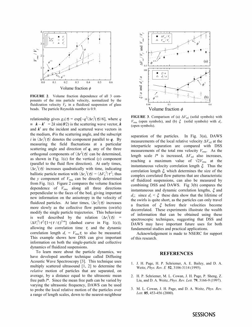
the y component of Vrms can be directly determinedfrom Fig. 1(c). Figure 2 compares the volume fractiondependence of Vrms along all three directionsperpendicular to the faces of the bed, giving importantnew information on the anisotropy in the velocity offluidized particles. At later times, H∆ri

2(τ)I increasesmore slowly as the collective flow patterns (swirls)modify the single particle trajectories. This behaviouris well described by the relation H∆ri

2(τ)I =H∆Vi

2Iτ.2/[1+(τ=/τc)2-m] (dashed curve in Fig. 1(c)),allowing the correlation time τc and the dynamiccorrelation length dc = Vrmsτc to also be measured.This example shows how DSS can give importantinformation on both the single-particle and collectivedynamics of fluidized suspensions.

To learn more about the particle dynamics, wehave developed another technique called DiffusingAcoustic Wave Spectroscopy [3]. This technique usesmultiply scattered ultrasound [1, 2] to determine therelative motion of particles that are separated, onaverage, by a distance equal to the ultrasonic meanfree path l*. Since the mean free path can be varied byvarying the ultrasonic frequency, DAWS can be usedto probe the local relative motion of the particles overa range of length scales, down to the nearest-neighbour

separation of the particles. In Fig. 3(a), DAWSmeasurements of the local relative velocity ∆Vrel at theinterparticle separation are compared with DSSmeasurements of the total rms velocity Vrms. As thelength scale l* is increased, ∆Vrel also increases,reaching a maximum value of √2Vrms at theinstantaneous velocity correlation length ξ. Thus thecorrelation length ξ, which determines the size of thecomplex correlated flow patterns that are characteristicof fluidized suspensions, can also be measured bycombining DSS and DAWS. Fig 3(b) compares theinstantaneous and dynamic correlation lengths, ξ anddc; since dc < ξ these data show that the lifetime ofthe swirls is quite short, as the particles can only travela fraction of ξ before their velocities becomedecorrelated. These experiments illustrate the wealthof information that can be obtained using thesespectroscopic techniques, suggesting that DSS andDAWS may have important future uses for bothfundamental studies and practical applications.

Acknowledgement is made to NSERC for supportof this research.

REFERENCES

1. J. H. Page, H. P. Schriemer, A. E. Bailey, and D. A.Weitz, Phys. Rev. E 52, 3106-3114 (1995).

2. H. P. Schriemer, M. L. Cowan, J. H. Page, P. Sheng, Z.Liu, and D. A. Weitz, Phys. Rev. Lett. 79, 3166-9 (1997).

3. M. L. Cowan, J. H. Page, and D. A. Weitz, Phys. Rev.Lett. 85, 453-456 (2000).

0.0 0.1 0.2 0.3 0.4 0.5 0.60

1

2

3

4

x

z

y

φ

Vy Vx Vz

φ 1/2

φ 1/3V rms /

V f

Volume fraction φ

FIGURE 2. Volume fraction dependence of all 3 com-ponents of the rms particle velocity, normalized by thefluidization velocity Vf, in a fluidized suspension of glassbeads. The particle Reynolds number is 0.9.

0.04 0.1 0.6

10

100

0.3

1

(b)

φ 1

ξ / a dc / a

φ -1/3

ξ /

a a

nd d

c / a

Volume fraction φ

(a)

φ 1

∆Vrel / Vf

Vrms / Vf

φ 1/3

∆Vre

l / V f a

nd V

rms /

V f

FIGURE 3. Comparison of (a) ∆Vrel (solid symbols) withVrms (open symbols), and (b) ξ (solid symbols) with dc.(open symbols).

A Non-Contact NDE Technique for Inspection ofRailroad Wheels

S. Jayaraman1, R. Alers2, B. Tittmann1

1Department of Engineering Science & Mechanics, Pennsylvania State University, University Park, PA 16802, USA.2Sonic Sensors, San Louis Obispo, CA, USA

A variety of defects like surface and sub-surface cracks in locomotive wheels might lead to their catastrophic failures. Hence, it isnecessary that the railroad wheels be inspected non-destructively regularly for the defects. This paper essentially concentrates onthe use of non-contact non-destructive techniques to inspect the locomotive wheels. The non-contact NDE technique employed iselectro-magnetic acoustic transducer (EMAT) method. Longitudinal and Shear wave EMATs were used to detect surface, sub-surface and internals flaws, depending on the flaw characteristics.

INTRODUCTION

Millions of tons of materials and waste are transportedon rails every year. There were more than 1500derailments in USA alone last year. The currentmethods for wheel crack detection are archaic, timeconsuming and require highly skilled operators toperform. None of the current methods can detect cracksbeneath the surface. All methods require at least 20hours of work per locomotive, as the wheels must beremoved and carefully cleaned. Considering what acritical role the integrity of the locomotive wheel playsin the safety of trains, it is vital that these methods beimproved. The biggest challenges for using a moreadvanced system to detect cracks in wheels are theneed to remove the wheel from the locomotive andclean it. The motivation for these experiments is (1) toevaluate the usefulness of the different wave modes indetecting surface and interior flaws and (2) to testperformance when intimate contact can not beachieved, because of possible residual deposits (dirt,oil, rust etc) on the tire walls.

EMAT TECHNIQUE

Non-contact NDE techniques have the advantage thatthe inspecting surface need not be cleaned. There areonly a few viable methods that can be used withoutcontact; we will focus on Eddy Current method andEMAT (Electromagnetic Acoustic Transducers)technique. EMATs are ultrasonic transmitters that donot need to have contact with the material to createstrong acoustic waves. A permanent magnet is placednear the surface of the sample, creating a magneticfield within the sample. A wire with an AC current isthen placed near the surface of the sample, creating analternating field within the sample, which creates eddycurrents. These eddy currents interact with the

permanent magnetic field and create deformations inthe material due to Lorentz force.

RESULTS

Experiments were conducted at the Penn StateUltrasonics laboratory on rail sections, and onlocomotive wheels at the Austrian OEBB. The resultsfrom both are presented below:

SAW EMATs

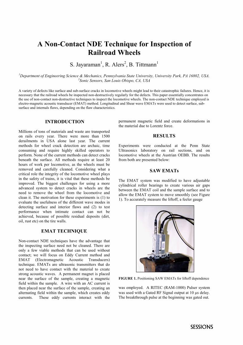
The EMAT system was modified to have adjustablecylindrical roller bearings to create various air gapsbetween the EMAT coil and the sample surface and toallow the EMAT system to move smoothly (see Figure1). To accurately measure the liftoff, a feeler gauge

FIGURE 1. Positioning SAW EMATs for liftoff dependence

was employed. A RITEC (RAM-1000) Pulser systemwas used with a Gated RF Signal output at 10 �s delay.The breakthrough pulse at the beginning was gated out.

A signal with a frequency of 1.01 MHz and amplitudeof 1.2 V was used as input to the EMAT system. Theintensity of the driving signal was damped by – 40 dB(or 10-4 less intensity) so that the signal could berecorded without overloading the oscilloscope. Thesignal was then recorded at a distance of about 32-mmwith several different liftoff positions. For low liftoff,the signal was clearly visible without much signalprocessing. However, for high liftoff, the signalwas much clearer for more signal summation averages.Therefore, for a low liftoff of 0.53 mm the signal wasonly summed over 7 signals (see figure 2), while for aliftoff of 1.2 mm the signal was summed for 100signals. Higher liftoff values than 1.2 mm did notprovide distinct peaks even with summations ofsignals.

FIGURE 2. Signal at liftoff of 0.53 mm (at 7 continuousaverages)

Normal Beam Shear Wave EMATs

It is possible to generate waves with a propagationdirection perpendicular to the surface (incident angle 0degrees), using normal beam EMATs. This isespecially useful for detecting interior cracks parallel tothe surface. Angle EMATs do have the disadvantagethat the reflected signal propagates to some other placedepending on the position of the flaw, but for someapplications this is very useful. An application specificnormal beam EMAT could be designed for pulse/echouse, which eases evaluation set-up.

Results from Austrian OEBB

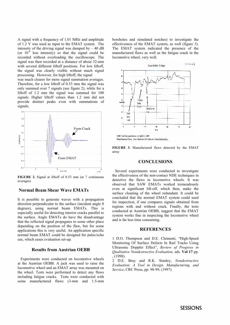
Experiments were conducted on locomotive wheelsat the Austrian OEBB. A jack was used to raise thelocomotive wheel and an EMAT array was mounted onthe wheel. Tests were performed to detect any flawsincluding fatigue cracks. Tests were conducted withsome manufactured flaws (3-mm and 1.5-mm

boreholes and simulated notches) to investigate theeffectiveness of the EMAT system, as well (figure 3).The EMAT system indicated the presence of themanufactured flaws as well as the fatigue crack in thelocomotive wheel, very well.

FIGURE 3. Manufactured flaws detected by the EMATarray

CONCLUSIONS

Several experiments were conducted to investigatethe effectiveness of the non-contact NDE techniques indetective the flaws in locomotive wheels. It wasobserved that SAW EMATs worked tremendouslyeven at significant lift-off, which then, make thesurface cleaning of the wheel redundant. It could beconcluded that the normal EMAT system could usedfor inspection, if one compares signals obtained fromregions with and without crack. Finally, the testsconducted at Austrian OEBB, suggest that the EMATsystem works fine in inspecting the locomotive wheeland is far less time consuming.

REFERENCES

1 D.O. Thompson and D.E. Chimenti, “High-SpeedMonitoring Of Surface Defects In Rail Tracks UsingUltrasonic Doppler Effect”, Review of Progress inQualitative Nondestructive Evaluation, eds. Vol 17 pp., (1998).2 D.E. Bray and R.K. Stanley, NondestructiveEvaluation: A Tool in Design, Manufacturing, andService, CRC Press, pp. 98-99, (1997).

From Crack

From EMAT

Applying of Sonoelasticity in Visualizingthe Internal Structure of a Composite

V. Chiroiua

aInstitute of Solid Mechanics, Romanian Academy, P. O. Box 1-863, Bucharest 70701, Romania

This is an attempt to solve the identification problem of the defect parameters on the basis of a free vibrating plate, for whichthe dimensions of the defect are comparable with the average grain size. The effect of shear waves is taken into considerationby considering a third-order theory for the displacement field.

1. IDENTIFICATION OF DEFECTS

Sonoelasticity is a technique, which combinesexternally applied vibrations with Doppler detection ofthe response throughout the medium for visualizing itsinternal structure (Gao, Parker and Alam [1]). Acomplete derivation of the micropolar elasticityequations was given by Eringen and Suhubi [2]. Thereare four basic waves traveling at four distinct phasevelocities into the plate. But only two coupled shearwaves have the wavelengths comparable to defects ofinterest. By writting the shear displacement vectoru and the microrotation vector � in terms of vector

potentials U and � u U� � � , �� �U 0 � �� � � , �� �� 0 (1.1)

these potentials must verify the equations( ) ,c c U c U tt2

232 2

32� � � � � ��

c U tt42 2

02

022� � � � � �� � � � � , (1.2)

where

c22��

� , c3

2��

�

cj4

2�

�

�, c5

2�

�� �

� , �

�

�02�

j (1.3)

The set C � {� � � � �, , , , } representsmaterial moduli, j is microinertia, vk is uk t, , � k t, .

We employ rectangular coordinates xk ( k � 1 2 3, , )or ( x x x y x z1 2 3� � �, , ).Suppose that the plane waves propagating in thepositive direction of the unit vector n have the form )](exp[0 vtrnikSS ��� (1.4)

where },{ �US � and },{0 BAS � with A B,

complex constant vectors, kv

�

�

the wave number

and r the position vector. Consider a plate of thicknessH , length a and width b . We suppose a small cube-defect cantered at ),,( 000 zyx with the side �a isembedded into the plate. The size of the defect iscomparable with the grain size and is characterized bya set of constants C0 � {� � � � � � �0 0 0 0 0 0 0, , , , , , }Over the whole medium we can write

),,(),,( 0* zyxCCzyxC �� (1.5)

���

�mediumsurrfor

defectforCzyxC

.,0,

),,( 00 (1.6)

Suppose that the defect is described by thecomponents: the centre ),,( 000 zyx , the side �a ,

and the set of parameters {� � �0 0 0, , }. Theobjective of the optimisation procedure is to minimisethe difference between the measured NFs

)(PQmes and the computed ones )(PQcalc where

}...{ 21 NQ ���� [3].

2. NUMERICAL RESULTS

For illustration we consider a polycrystalline metalplate whose grain size is approximately05 10 5. �

� m . In order to simplify the numericalstudies we suppose that this material is characterizedby� �� � 40GPa ,� � 0 2. GPa ,� � �� � � 3GN ,

j m� ��6 25 10 7 2. and � � 1160 3Kg m/ . The

plate dimensions are: a mm� 100 , b mm� 110 ,H mm� 2 . Consider a cubic defect of the side

� �a 2 10 5�

� m , located in ( , , )15 15 0� , andcharacterized by � �0 4� � , � �0 4� � ,� �0 � , � �0 � , � �0 � , � �0 � and� �0 15� �. . We have:x0 15 9� . , y0 14 2� � . , z0 0� ,

� �a 2 9 10 5. �� m ,� �0 4 2� �. ,

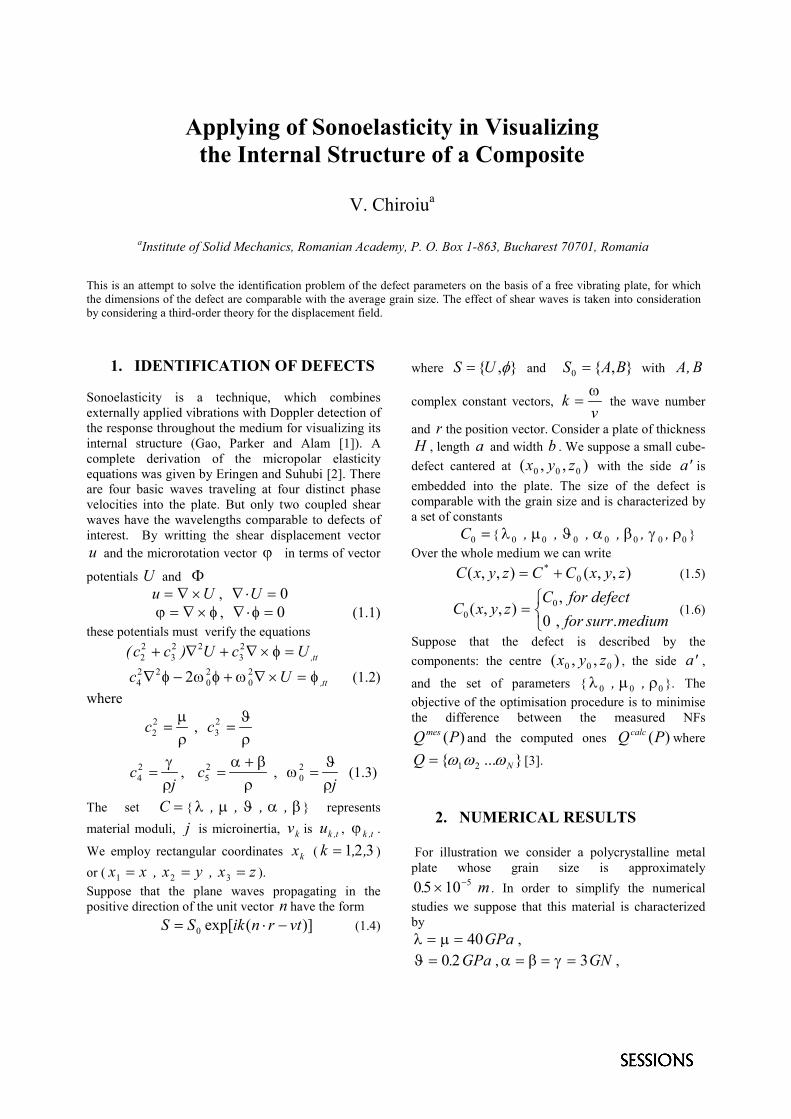
� �0 381� �.and � �0 168� �. . In figure 1 snapshots of thenondimensionless displacement and microrotationamplitudes at 100�t �s as functions ofnondimensionless spatial coordinates are displayed.

FIGURE 1 Snapshots of displacement and microrotation amplitudes at 100�t s as functions of spatial

coordinates

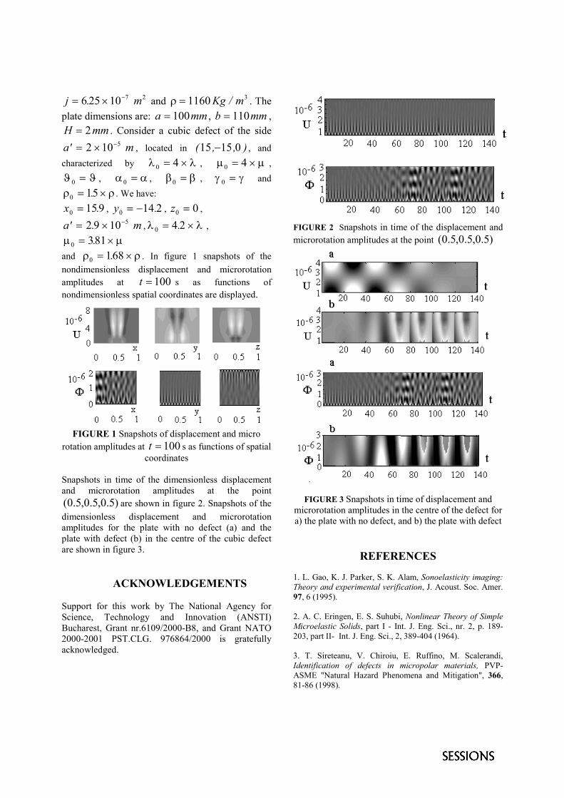
Snapshots in time of the dimensionless displacementand microrotation amplitudes at the point

)5.0,5.0,5.0( are shown in figure 2. Snapshots of thedimensionless displacement and microrotationamplitudes for the plate with no defect (a) and theplate with defect (b) in the centre of the cubic defectare shown in figure 3.

ACKNOWLEDGEMENTS

Support for this work by The National Agency forScience, Technology and Innovation (ANSTI)Bucharest, Grant nr.6109/2000-B8, and Grant NATO2000-2001 PST.CLG. 976864/2000 is gratefullyacknowledged.

FIGURE 2 Snapshots in time of the displacement andmicrorotation amplitudes at the point )5.0,5.0,5.0(

FIGURE 3 Snapshots in time of displacement andmicrorotation amplitudes in the centre of the defect fora) the plate with no defect, and b) the plate with defect

REFERENCES

1. L. Gao, K. J. Parker, S. K. Alam, Sonoelasticity imaging:Theory and experimental verification, J. Acoust. Soc. Amer.97, 6 (1995).

2. A. C. Eringen, E. S. Suhubi, Nonlinear Theory of SimpleMicroelastic Solids, part I - Int. J. Eng. Sci., nr. 2, p. 189-203, part II- Int. J. Eng. Sci., 2, 389-404 (1964).

3. T. Sireteanu, V. Chiroiu, E. Ruffino, M. Scalerandi,Identification of defects in micropolar materials, PVP-ASME "Natural Hazard Phenomena and Mitigation", 366,81-86 (1998).

On Estimating Concrete Porosity by Ulrasonic Non-Destructive Testing

L.Vergaraa, R.Mirallesa, J.Gosálbeza, F.J.Juanesa, L.G. Ullateb, J.J. Anayab, M. G.Hernándezb, M.A.G. Izquierdob

aETSI Telecomunicación , Univesidad Politécnica de Valencia,Camino de Vera s/n, 46022 Valencia, EspañabInstituto de Automática Industrial (CSIC), La Poveda,28500, Arganda del Rey , Madrid, España

Premature damage of mortar and concrete structures, due to environmental action, demands procedures to estimate durability ofthis type of components. Mortar or concrete composition (e.g., grain size, type and percentage of sand) may have some influencein the durability, but it is mainly related to porosity, which determines the interaction between aggressive agents and material. Inthis work, several NDE ultrasonic methods to estimate porosity of mortar are presented and evaluated. In these methods porosityis related to (1) the material structural noise, (2) sound velocity and (3) ultrasonic attenuation. In all these methods mortar isconsider to be formed by only two phases: solid and pores.

INTRODUCTION

In recent years, an increase in the number ofstructures presenting symptoms of premature damagehas taken place due to the action of different aggressiveprocesses. This has made necessary to improve thescientific knowledge of the physical and chemicalmechanisms which deteriorate the concrete, as much asof the procedure to evaluate its durability, in order tomitigate the high cost of repairing and maintenance ofthese structures. The processes that affect the durabilityof concrete are mostly related to its porous structure,which determines the interaction between concrete andits environment. Pores and capillaries in the interior ofconcrete will propitiate destructive processes, whichcommonly start on the surface. in the penetration ofaggressive agents since it has no contact with theexterior. Due to the complexity of concrete, it was decided tostart analysing a simpler substance like mortar. For theexperimental verification, there has been prepared a setof 120 mortar probes with normalised sand (prisms of asize of 16x4x4 cm) adjusted to the water percentageused in the preparation of cement paste. Fivepercentages of water/cement were taken into account:0.45, 0.50, 0.55, 0.60, and 0.65. Thus, generating 24probes for each percentage; 12 of which were used toconduct destructive tests of porosity measure; 6 for theNDE grain noise approach and 6 for NDE based onvelocity and attenuation analysis. Varying the waterpercentage in the cement paste is an easy and reliableprocedure to obtain different porosity levels. Theprobes were made by AIDICO (Instituto Tecnológicode la Construcción, Valencia, Spain), which was alsoresponsible to perform the destructive testing to verifythe actual porosity of the probes .

CHARACTERISATION BASED ONSTRUCTURAL NOISE

The first work consisted in the extraction ofstatistical parameters of the ultrasonic signal, linked tothe pulse spectrum (instantaneous frequency,bandwidth, cepstral and correlation analysis,...). Toillustrate this, figure 1 shows the average dependencybetween the first value of the cepstrum sequence andthe water/cement percentage. Cepstral analysis is onethe standard procedures for extracting pulseinformation from material or tissue structural noise [1].The transducer frequency was 1MHz and the samplingfrequency 5MHz. The curves are the result ofaveraging ten measures, taken on each probe for eachwater/cement percentage. Alike curves were obtainedfrom other spectral parameters. In a general manner,clear tendencies in the variation of the parameters withwater/cement percentage are observed. Nevertheless,not with the grade of monotonicity (increasing ordecreasing) that would be necessary to determine aprecise technique of porosity measure. It should benoted that the average grain size in all the probes wasthe same.

FIGURE 1. Cepstrum coefficient versus water-cement ratio

CHARACTERISATION BASED ON THEVELOCITY OF SOUND

To apply a micro-mechanic model to the mortar, weconsider the material to be formed by a solid phase,which occupy a volume Vm, plus the pores, whichoccupy a volume Vi (Vm +Vi=1). We also consider thatthe capillary pores (of a size inferior to the micron)have a cylindrical and extended shape, and that itsdistribution is random in the solid phase. Starting fromthese hypotheses, an expression can be achieved thatrelated the velocity of propagation in the medium withporosity [2], as follows:

),,,( , XTCfv klmnm

ji ρ= (1)

where v indicates the propagation velocity of theacoustic waves. Cm

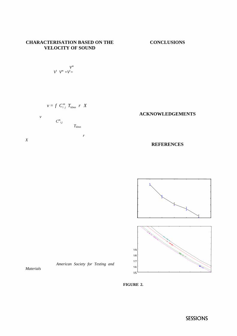
i,j determine the constants ofelasticity of the solid phase, Tklmn indicates the tensorterms which contain the size, distribution andorientation of pores in the material, ρ is the density andX the porosity percentage. The average velocity has been measured on the sixprobes of each group, by means of two transducersoperating in transmission, in dry, and using a contact ofrubber. Three points per probe have been measured.Figure 2a shows, for a 1 MHz transducer, thedistribution of measures per groups of probes, and thestandard deviation of measured values in each group.As can be seen, the velocity of propagation is aparameter capable of discerning the groups of probeswith different water/cement percentages. In 2b it canbe seen curves that relate porosity and velocityregarding the micro-mechanic model. Each curve hasbeen obtained by finding the parameters of the model(1) for each water-cement percentage group of probes.For finding the model parameters we need the averageporosity measure obtained by destructive methods in agiven group, and the average velocity obtained byNDE ultrasonic methods in the same group. Note infigure 2b that each group produces a different modelfitting, although the curves are close enough to give apromising method for a precise measure of porosity.On them have also been drawn the points obtainedfrom the measure of porosity by destructive methods(circles) and measure of velocity by means ofultrasonic (x). The destructive technique for measuringthe porosity is the one described in the standard ASTMC 642-90 of the American Society for Testing andMaterials.

CONCLUSIONS

Two ultrasonic methods to estimate porosity in mortarhave been presented. The method based on the velocityof acoustic propagation offers satisfying results forestimating porosity in mortar. On the other hand, themethods based on structural noise, and on attenuationof material present clear tendencies. Yet, not with theprecision that would be necessary to be considered areliable technique to measure porosity. Applying thesame methods to an actually two-phase material (e.g.hydrated cement mass) we will be able to reach thescientific knowledge of the procedures to evaluatedurability in composite cements

ACKNOWLEDGEMENTS

This work has been supported by SpanishAdministration under grants CICYT TAP97-1128 andDPI2000-0619.

REFERENCES

1. Jensen JA, Leeman S. Nonparametric Estimation ofUltrasound Pulses, IEEE Trans. on Biomedical Engineering1994; 41(10):929-936.2. Hernandez MG, Izquierdo MA, Ibáñez A, Anaya JJ,Gómez-Ullate L. Porosity estimation of concrete byultrasonic NDE. Ultrasonics 2000; 38:531-533.

FIGURE 2. a) Velocity measures of the 5 groups ofprobes. b) Theoretical curves of porosity -- applyingthe micro-mechanic model

3600

3700

3800

3900

4000

4100

4200

45 50 55 60 65

a)

3500 3600 3700 3800 3900 4000 4100 420015

16

17

18

19

20

21

22

23

45%

50%

55%

60%65%b)

Using HF Ultrasonic Shear Waves for Determination ofElastic Properties of Fresh Special Concrete

R. Čopa and M. Maletićb

aUniversity of Ljubljana, Faculty of Maritime Studies and Transport, 6320 Portoroz, SloveniabUniversity of Zagreb, Faculty of Electrical Engineering and Computing, 10000 Zagreb, Croatia

Testing methods should be quick, with the low costs, combined with a high accuracy and performed by the well-qualifiedexperts with long experience. All non-destructive methods in the civil engineering are new but the variety of tasks and testingtechniques are enormous. Testing methods for measuring the properties of a fresh concrete are of special interest because it ispossible to predict the properties of concrete prior to its placement on the basis of its results. Particularly exciting isestablishing the correlation between these new methods and the standard mechanical tests. Such type of testing method needsto be developed.

THE SEARCH FOR THE NEWTESTING METHODS

According to the definition agreed upon by RILEM'sTechnical Committee TC 145-WSM, special freshconcrete is such concrete which, in its fresh state,cannot be adequately assessed by one or morecommon standard workability tests.

The interaction between the material and theultrasound could be used to obtain information on thematerial structure. Generally, a wide range of thematerial parameters could be determined by ultrasonicmeans but some of them, such as the elastic moduli,are really well established [1].

Propagation of the Ultrasonic WavesThe propagating velocity of the ultrasonic longitudinalwaves’ sound pulses, passing through the fresh mortar,will start to diminish almost immediately after themixing of a mortar has been finished. The researcherscould make their measurements even fifteen minutesbefore the end of the induction period [2]. In thisinitial period the concrete matrix is still in the state ofsolution sol. About two hours after the mixing of amortar has been finished, the maximum rate of changeof the sound pulses velocity occurred and it showedthe increase of velocity; such change took place beforethe significant amount of hydration products has beenformed, and much earlier then the increase ofpenetration resistance has started. About less than fivehours after the mixing of a mortar has been finished,the penetration resistance started to increase rapidly.

At that time the compressive strength has just began todevelop [3].

REFLECTION OF THE ULTRASONICSHEAR WAVES

This method is based on the ultrasonic shear wavesreflection from the upper layer of the hardeningcement paste. For the choice of the right wave length λthe Rayleigh scattering criteria is accepted: λ > d,where ‘d’ is the maximum grain size. To avoid zeroerrors the amplitudes of the incident wave and the firstreflected wave are measured [4].

The shear modulus of elasticity and the viscosity aredetermined by the acoustic attenuation of the normalincident waves and the reflected waves. It changes inthe course of the hydration process. The amplitude ofthe incident waves A1, amplitude of the reflectedwaves A2 and their related phase Φ were measured.The reflection coefficient r0 (Eq.1) and the complexreflection coefficient r were calculated.

2 2 10

1 2 1

(1)A Z ZrA Z Z

−= =+

Z R iX= + Complex optical impedance2 2( ) (2)G R X ρ= −

The error of omitting Φ is insignificant for themagnitude of shear elastic modulus G [5]. For thisreason the set-up for ultrasonic measuring shear elasticmodulus G is more simple (Eq.2). This kind ofconfiguration of the measuring set-up has been usedalso by other researchers [6].

FIGURE 1. Set-up of the simple and law-costultrasonic measuring system.

An Experimental System And ResultsThe personal computer was used as a systemsupervisor and a storage unit. It was also used as aninitial trigger for the signal generator and anoscilloscope (Fig.1). So, the probe excitation pulsescoincided with the samples of data. In order toimprove the signal-to-noise ratio, waveform averagingwas performed by an oscilloscope, which was appliedfor the signal analysis as well.

FIGURE 2. The change of a shear modulus duringthe hydration of a pure Portlant cement.

The slope dr0/dt of the hydration process r0 = f (t)defines the geometry of the grain growth (Fig.2). Thisderived from the kinetic model of Avrami [7] andcoincides with the scanning electron microscopy of thecement paste hydration [3]. The maximum value r0 = f(t) correlate with the mechanical properties of ahardened concrete. To consider such correlation agood repetition of the measuring results is to beassured. The external pressure has the greatestinfluence on the buffer. For this reason we started to

make all our samples of the cement mortar in the samegeometrical size and of the same weight.

The signal analysis is performed in the last step bypartitioning the signal into the discrete windows in thetime domain what refers to the appearance of theincident and reflected waves in the order as theypassing through a medium. Further, this windows areto be transformed into the frequency domain foradditional filtering and interpretation. The number ofthe discrete frequency bands is defined (Eq.3):

( )1 2

21 (3)2

n

RMSm

V Xω

ω=

= ∑

The initial experimental studies has shown that, bothappearance and decay of the discrete frequency bandsdepend upon the composition of the substance whichhas been tested. Consequently the composition of aconcrete mortar could be find out, on the bases of itssample test and subsequently frequency domain signalanalysis.

CONCLUSIONEvery testing method has the two aspects: theresearcher’s point of view and the contractor’s point ofview. The applicable testing method should combinethe both of them: should be quick, with the low costs,with a high accuracy and performed by the well-qualified experts with a long experience.

REFERENCES[1] SMITH, R.L. Ultrasonic materials characterization.

NDT International, February 1987, vol.20, n.1,p.43-48.

[2] KEATING, J. et al. Comparison of shear modulusand pulse velocity techniques to measure the build-up of structure in fresh cemente pastes used in oilwell cementing. Cement and Concrete Research.1989, vol.19, p.554-566.

[3] CASSON, R.B. et al. The use of ultrasonicvelocity, penetration resistance and electronmicroscopy to study the rheology of fresh concrete.Edit by Skalny J. Cocrete Rheology. Boston:Materiels Research Society, Nov.1982, p.66-75.

[4] KRAUTKRÄMER, J., KRAUTKRÄMER, H.Ultrasonic testing of materials. 2nd ed. Berlin:Spring-Verlag, 1969, p.460-466.

[5] STEPIŠNIK, J., LUKAČ, M., KUCUVAN, I.Measurement of cement hydratation by ultrasonics.Ceramic Bulletin. 1981, vol.60, no.4, p.481-483.

[6] D'ANGELO, R. et al. Method for measuringcement thickening times. Unitet States Patent, 5412 990. 1995, May 9.

[7] BURKE, J. The kinetics of phase transformationsin metals. Oxford: Pergamon Press, 1965.

0 10 20 30 40 500 ,0

0 ,1

0 ,2

0 ,3

0 ,4

0 ,5

0 ,6

0 ,7

0 ,8

0 ,9Hydration of portlant cement PC 52.5rw/c=0,4; humidity 96%

r 0 = A

2/A1

Time t [hours]

Advances in Air-coupled Ultrasonic Testingin the Frequency Range 750 kHz to 1 MHz

E. Blomme, D. Bulcaen and F. DeclercqKatholieke Hogeschool Zuid-West-Vlaanderen, dept. VHTI

Doorniksesteenweg 145, 8500 Kortrijk, Belgium

Non-contact air-coupled ultrasonic measurements and imaging experiments are presented in a wide range of materials such ascoated textile, aluminium, thin casting and spot welds on steel. All measurements have been performed by either frequencyswept sinusoidal signals or modulated chirp signals in the frequency range 0.75 – 1 MHz using piezoelectric transducers withmatching layers.

INTRODUCTION

The advantage of ultrasonic NDT is well known: itis applicable to almost all kinds of matter, transparentor not, it requires none or very few preparation of thesample, it is versatile, non-hazardous, safe andrelatively inexpensive. On the other hand, ultrasonicNDT suffers from a severe limitation: all conventionalmethods are either contact or immersion techniques.As a consequence, most ultrasonic methods do notcome into consideration for on-line testing.

This is changing… Thanks to the progress in non-contact ultrasonic technology, contact-free ultrasonicinspection, evaluation and imaging methods are beingdeveloped. In the present contribution, recentexperiments are reported with respect to air-coupledultrasound applied to a wide diversity of materials.

THE MEASUREMENT SYSTEM

The air-coupled piezoelectric transducers (typeULTRAN, NCT-series of Ultranlabs, Second WaveSystems) have been implemented into two differentelectronic systems: a first system operating incontinuous mode, a second system in pulse mode. Inthe former case, frequency-swept sinusoidal signals areapplied and each point of a B- or C-scan results from apeak amplitude. In the latter case, use has been madeof NCA1000, an ultrasonic pulser/receiver instrumentfrom VN Instruments Ltd. based upon the synthesis ofa computer generated chirp and pulse compressionalgorithms [1]. In this case, each point of a scan resultsfrom an integrated response [2]. All results have beenobtained in transmission mode at sound frequenciesbetween 0.75 and 1.03 MHz and at normal incidence ofthe sound beam. In all cases, the air gap at transmitterside was between 2 and 3 cm and at receiver sidebetween 0.5 and 1 cm.

EXPERIMENTS

We shall report here on some experiments dealingwith various (flat) materials, i.e. materials with aparallel front and backside. Related examples andadditional comments can be found elsewhere [1,2].

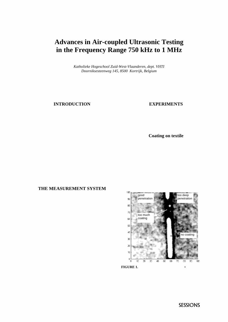
Coating on textile

Figure 1 shows a non-contact C-scan based oncontinuous 1 MHz air-coupled ultrasound of a piece oftextile on which a protecting coating has been appliedone-sidedly (80 g/m²). On the right part, too muchpressure was exercised resulting into too deeppenetration of the coating into the textile. On the leftpart, the coating was applied correctly. A strip with toomuch coating separates both regions. The left and rightpart can be clearly distinguished from each other (notethe difference in gray level).

FIGURE 1. C-scan of a piece of textile (100 × 100 mm) one-sidedly coated (f = 1 MHz, continuous mode, T: ∅ 12.5 mm,R: ∅ 3 mm).

goodpenetration

too deeppenetration

too muchcoating

no coating

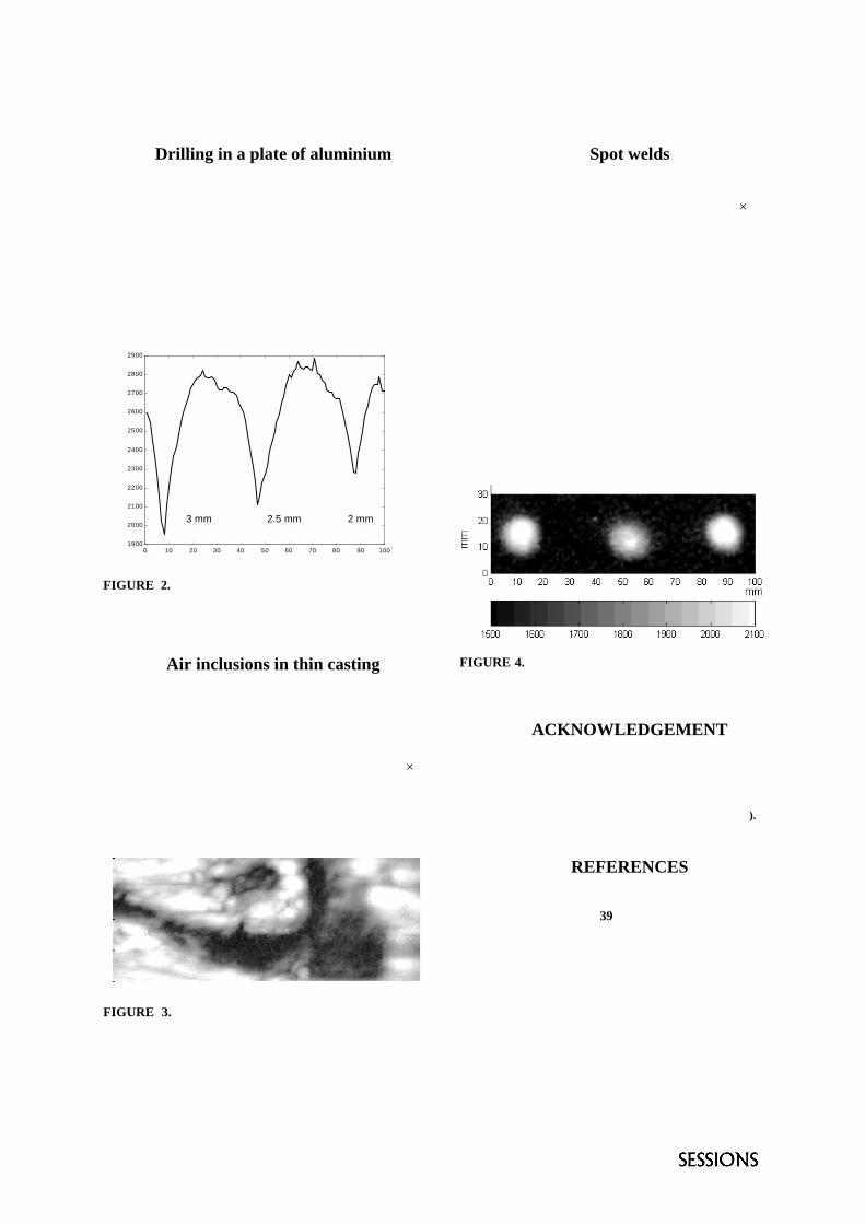
Drilling in a plate of aluminium

Figure 2 shows the result of a B-scan along analuminium plate of 8 mm thickness in which laterally 3cylindrical holes are drilled with different diameters (2,2.5 and 3 mm). In this case ultrasonic chirps have beenused of centre frequency 0.76 MHz and 200µs pulseduration. The reduction of the received signal (thestrongest at ∅ 3 mm) is significant. The example isrelevant in view of the detection of flaws in materialswith high acoustic impedance.

FIGURE 2. Line scan along a 100 mm long area of analuminium plate containing 3 holes of resp. diameter 3, 2.5and 2 mm; the vertical scale refers to arbitrary units (f = 0.76MHz, pulse mode, T: ∅ 12.5 mm, R: ∅ 3 mm);

Air inclusions in thin casting

This example opens interesting perspectives for thenon-contact inspection of thin castings. The black areason the C-scan in figure 3 reveal a pattern of many tinyair inclusions in a zamac plate (an alloy of zinc andaluminium) of 2 mm thickness over an area of 7 × 4cm. The image has been obtained by continuousultrasound of 1.03 MHz, which is one of the resonantfrequencies of the plate.

FIGURE 3. C-scan of a zamac plate with a pattern ofhundreds of small air inclusions (f = 1.03 MHz, continuousmode, T: ∅ 12.5 mm, R: ∅ 3 mm).

Spot welds

The last example deals with spot welds on steel. Infigure 4, a C-scan is shown of an area of 10 × 3 cmfrom a plate consisting of two sheets of steel (1mm +3 mm) joined together by 3 spot welds (∅ 6 mm). Themiddle spot has been applied at 50% of the electriccurrent and hence is of less quality (although stillacceptable as local melting of the sheets is established).The scale refers to arbitrary amplitude units. The weldof decreased quality can clearly be distinguished (notethe significantly lower brightness of the spot). Thedark areas between the welds demonstrate the very badtransmission at places where no melting takes place.There the sheets of steel are not bounded and separatedby an air layer. In view of the high acoustic impedanceof steel, this result is very promising for non-contacton-line testing of spot weld quality, provided thesample is accessible from both sides.

FIGURE 4. C-scan of 3 spot welds on steel (f = 0.75 MHz,continuous mode, T: ∅ 12.5 mm, R: ∅ 12.5 mm).

ACKNOWLEDGEMENT

Work supported by the Institute for the Promotionof Innovation by Science and Techology in Flanders(IWT) and several Flemish companies within theframework of HOBU-Fund projects (980076/000197).

REFERENCES

1. T.H. Gan, D.A. Hutchins, D.R. Billson and D.W.Schindel, Ultrasonics 39,181-194 (2001).

2. E. Blomme, D. Bulcaen and F. Declercq, “Air-coupledultrasonic NDE: experiments in the frequency range 750kHz to 2 MHz”. Accepted for publication in NDT&EInternational.

0 10 20 30 40 50 60 70 80 90 1001900

2000

2100

2200

2300

2400

2500

2600

2700

2800

2900

∅ 3 mm ∅ 2 mm∅ 2.5 mm

Lamb wave conversion at the bevelled edge of a plate.

Nicolas Wilkie-Chancellier, Hugues Duflo, Alain Tinel and Jean Duclos

Laboratoire d'Acoustique Ultrasonore et d'Electronique (L.A.U.E), CNRS (UMR 6068),Université du Havre, Place Robert Schuman, BP 4006, 76610 Le Havre, France

e.mail : nicolas.wilkie@iut.univ-lehavre.fr

The theory of Lamb wave in a plate and the wave reflection at a free edge is well known. This paper presents an experimentalstudy of mode conversions that occur when an incident wave is reflected at the straight edge of a plate. Then, the results arecompared to numerical computations (Finite element method). A Lamb mode is excited in a steel plate (A1 mode) and the normalcomponent of surface wave displacements is measured with a laser vibrometer. These displacement values are connected with thewave power flow to perform an energy balance. The propagation of an incident wave (A1 mode) in a steel plate and its reflectionon the bevelled edge of the plate is also simulated by a finite element calculation for several angles.

Introduction

Lamb waves [1] are frequently used for nondestructive evaluation of plane structures because theyare propagating without attenuation if the structure islocated in the vacuum. In practice, structures havefinite dimensions. Several researchers have tried toexplain this phenomenon. Studies have been realised tostudy Lamb wave propagation and their reflection on astraight edge of a plate. We present an experimentalstudy of Lamb wave conversion at the straight free endof a plate in vacuum. Then, the propagation of Lambmodes and their reflection at the extremity aresimulated by the finite element method (F.E.M.) toconfirm experimental results. Then, several results arepresented for various plates bevelled at differentangles.

Experimentation

In order to study the Lamb mode conversion at theend of a plate, we realise the following experimentalset-up. The description of the bevelled plate is shownin Figure1.

x3

x1

x2

α

FIGURE 1. Description of the bevelled plate.

A pulse generator sends a tension pulse to a piezo-composite emitting transducer. The transducer is set upon a Plexiglas wedge inclined with regard to thenormal of plate surface to generate a wave. Thetransducer inclination is selected to obtain a particularLamb mode. We use a He-Ne laser vibrometer tomeasure normal displacements on the plate surface byinterferometry. The laser vibrometer is installed on an

orthogonal translation, which allow complete scan of aline (in the Ox1 direction) on the surface plate by 0.2mm step. The temporal signal, visualised by anumerical oscilloscope, is transmitted to a computerand stored. After the acquisition of the temporal signal at eachposition, we compute two successive Fouriertransforms, one temporal and the other spatial, in orderto observe Lamb modes in the dual space [2]. Then, wecan represent the Lamb mode amplitudes versus wavenumber K for a given thickness-frequency product.This representation allows recognising differentmodes. The amplitude of a Lamb mode is connected tothe corresponding energy by the relation that existsbetween the normal displacement on surface plate andthe Poynting vector flow through a straight section ofthe plate. After this treatment, we plot the convertedmodes energies curves when the t A1 mode is incident.An experimentation has been realised with α=90°.Results are shown in third part.

Finite elements calculation

A transient analysis method is performed. Thestudied plate is isotropic. Then, a two-dimensionalmesh is modelled (Ox1x2) to describe Lamb wavepropagation, which is not associated to stresses ordisplacements in the third direction. The mesh iscomposed of plane elements with four nodes. Thestudied inoxydable steel plate is 40 mm long and 2 mmthick. Its caracteristics are: E=2,0043.1011 N.m2

(Young Modulus), υ=0,29 (Poisson coefficient),ρ=7800 kg.m-3 (density). To generate a Lamb mode in the plate, we use thedisplacements related to this mode which aretheoretically computed at any point in the thickness ofthe plate. Indeed, Torvik [3] had suggested that thewaves, propagating in a plate into vacuum, are thesame as the waves in the infinite plates. The normal

and tangential components of the Lamb wavedisplacements are imposed on nodes at the end of theplate (x1=0). These components vary sinusoidally inphase quadrature. Five periods are applied to perform aquasi-harmonic study. The interest of this technicgeneration is that it needs no distance for Lamb modeestablishment. Indeed, for the nodes near from the endof the plate, the wave seems to be propagated on aninfinite plate. We collect the normal displacements onthe surface of the plate and we use the same treatmentas for the experimentation. Then we can executeenergy balances for the bevelled plate. Calculationshave been realised with plates bevelled at differentangles (α=90°, 85° and 80°).

Results

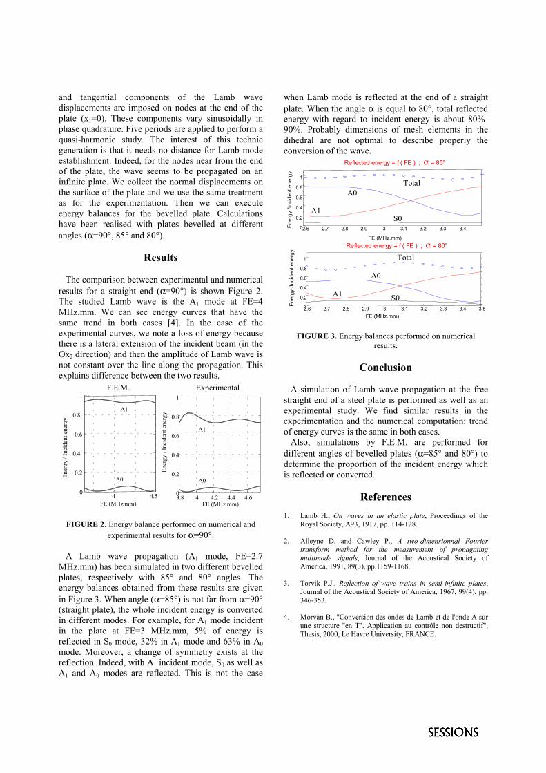
The comparison between experimental and numericalresults for a straight end (α=90°) is shown Figure 2.The studied Lamb wave is the A1 mode at FE=4MHz.mm. We can see energy curves that have thesame trend in both cases [4]. In the case of theexperimental curves, we note a loss of energy becausethere is a lateral extension of the incident beam (in theOx2 direction) and then the amplitude of Lamb wave isnot constant over the line along the propagation. Thisexplains difference between the two results.

3.8 4 4.2 4.4 4.60

0.2

0.4

0.6

0.8

1

FE (MHz.mm)

Experimental

A1

A0

Ene

rgy

/ Inc

iden

t ene

rgy

FE (MHz.mm)

Ene

rgy

/ Inc

iden

t ene

rgy

4 4.50

0.2

0.4

0.6

0.8

1

A1

A0

F.E.M.

FIGURE 2. Energy balance performed on numerical andexperimental results for α=90°.

A Lamb wave propagation (A1 mode, FE=2.7MHz.mm) has been simulated in two different bevelledplates, respectively with 85° and 80° angles. Theenergy balances obtained from these results are givenin Figure 3. When angle (α=85°) is not far from α=90°(straight plate), the whole incident energy is convertedin different modes. For example, for A1 mode incidentin the plate at FE=3 MHz.mm, 5% of energy isreflected in S0 mode, 32% in A1 mode and 63% in A0

mode. Moreover, a change of symmetry exists at thereflection. Indeed, with A1 incident mode, S0 as well asA1 and A0 modes are reflected. This is not the case

when Lamb mode is reflected at the end of a straightplate. When the angle α is equal to 80°, total reflectedenergy with regard to incident energy is about 80%-90%. Probably dimensions of mesh elements in thedihedral are not optimal to describe properly theconversion of the wave.

FE (MHz.mm)

En

erg

y /I

ncid

ent

en

erg

y

Reflected energy = f ( FE ) ; α = 85°

2.6 2.7 2.8 2.9 3 3.1 3.2 3.3 3.40

0.2

0.4

0.6

0.8

1

S0A1

A0Total

2.6 2.7 2.8 2.9 3 3.1 3.2 3.3 3.4 3.50

0.2

0.4

0.6

0.8

1

FE (MHz.mm)

En

erg

y /I

ncid

ent

en

erg

y

Reflected energy = f ( FE ) ; α = 80°

S0A1

A0

Total

FIGURE 3. Energy balances performed on numericalresults.

Conclusion

A simulation of Lamb wave propagation at the freestraight end of a steel plate is performed as well as anexperimental study. We find similar results in theexperimentation and the numerical computation: trendof energy curves is the same in both cases. Also, simulations by F.E.M. are performed fordifferent angles of bevelled plates (α=85° and 80°) todetermine the proportion of the incident energy whichis reflected or converted.

References

1. Lamb H., On waves in an elastic plate, Proceedings of theRoyal Society, A93, 1917, pp. 114-128.

2. Alleyne D. and Cawley P., A two-dimensionnal Fouriertransform method for the measurement of propagatingmultimode signals, Journal of the Acoustical Society ofAmerica, 1991, 89(3), pp.1159-1168.

3. Torvik P.J., Reflection of wave trains in semi-infinite plates,Journal of the Acoustical Society of America, 1967, 99(4), pp.346-353.

4. Morvan B., "Conversion des ondes de Lamb et de l'onde A surune structure "en T". Application au contrôle non destructif",Thesis, 2000, Le Havre University, FRANCE.

Effect of Laser Intensities on Transient ThermalDeformation of Alumina (Al2O3) Substrate

S. Jayaraman, R. Halter, B. Tittmann

Department of Engineering Science & Mechanics, Pennsylvania State University, PA 16802, USA

One of the major problems during the laser drilling process in the electronic component industry has been identified as thecracking and failure of the ceramic substrates. The cracking and failure is due to large localized thermal stresses within thenarrow heat-affected zone on the ceramics. An electronic speckle pattern interferometer (ESPI) system was designed and used totake speckle pattern images of the ceramic surface during the laser drilling process. Two different laser intensities were used fordrilling and the deformation of the ceramic was observed to be different in each of the case. Using commercial software, thespeckle fringe images were image processed to quantify whole-field transient out-of-plane displacement measurements.

1. INTRODUCTION

Laser machining has been used to heat treat, cut,weld, and drill electronic ceramics by the electronicmanufacturing industries in particular [1 Because of theproperties of ceramics, the large, focused heat fluxrates which allow material melting and ablation, mayalso produce large localized thermal stresses within thenarrow heat-affected zone, which can lead to micro-cracks, significant decreases in strength, and evencatastrophic failure during the shaping process [2].Monitoring the thermal stresses in ceramic specimensduring the laser shaping process directly is a difficulttask. Measuring the transient deformation however,may be an alternative solution. There are numerousmethods for measuring deformation in general. Opticalmethods such as electronic speckle patterninterferometer (ESPI) have the advantages of beingnon-contact, having high temporal resolution, and withthe inclusion of a microscopic lens, are able tovisualize small areas of interest.

2. PRINCIPLE OF FRINGEFORMATION

When two interfering electromagnetic waves (such asthe reference and object beams in an interferometer),having some fixed-phase relationship relative to oneanother, are superimposed, the result is referred to asinterference. If two speckle patterns are subtracted oradded, fringe patterns will be observed. Since thephase difference ��(r) is a function of thedisplacement of the object surface, information aboutthe relative displacement of different parts of thesurface can be obtained from the position of thespeckle fringes. Brightness on the TV monitor thatshows subtracted images of the speckle pattern isminimum when ��(r) = 2n�, n = 0,1,2,3… as dark

lines. Phase difference, ��(r) due to displacement d atany point on the object surface can be related to thispath difference � by:

This equation gives the relationship between thephase difference and the displacement vector d. For theoptical system, the probed phase change due todisplacement may be expressed by

where z is the out-of-plane component of displacementvector d, �1 is the angle of the object beam to thesurface normal (z-axis) and �2 is the angle of theobservation direction to the surface normal (z-axis).

3. EXPERIMENTAL SETUP ANDPROCEDURE

The specimens used were aluminum oxide (Al2O3)wafers and were chosen because of their importance tothe electronic industry [source]. Each specimen was athin circular wafer with a radius of 25 mm and athickness of 0.5 mm. A 1.5 kW (max power) CO2laser (Coherent General) and a 60 W (max power)CO2 laser were used as the drilling beams andimpinged perpendicularly upon the specimen. Theprocedure consisted of drilling the specimen with aCW beam for 200 milliseconds in case of higherintensity and for 4 seconds in the case of lowerintensity laser, and capturing the speckle images usingthe designed MESPI system. The design can be dividedinto two parts: optical and electronic. Optical

� � ��� drλπ2∆φ

� � � �21A cosθθ coszλ2πr∆ ��φ

(1)

(2)

components consisted of a laser, mirrors, long distancemicroscope, polarizer, spatial filters, and beamsplitters. The electronics consisted of a CCD camera,PCI interface board, and a PC. A NEWPORT portableoptical table, with vibration isolation legs, was used tohouse the system in order to provide a portable andvibration free environment. A He-Ne laser, with anapproximate output power of 15 mW at a wavelengthof 632 nm, was used as the light source. An Infinitymodel K-2 long distance microscope was used to viewthe drilling area. A spatial filter, consisting of an iris,microscope objective and a pinhole, was used to cleanthe beam, creating a smooth and nearly ideal Gaussianintensity profile. The CCD camera offered a double-exposure feature that created two exposures on a singleimage. A fringe skeleton method was used to separateand analyze the fringe patterns obtained directly fromthe double exposed image. This analysis wasaccomplished using Adobe Photoshop™ and theFringe Processor™ developed by the Bremen Instituteof Applied Beam Technology.

4. RESULTS AND DISCUSSION

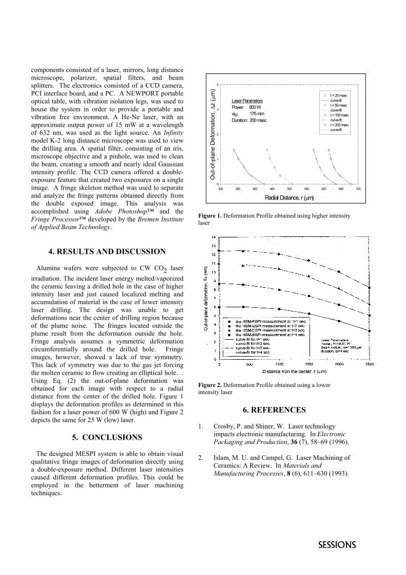
Alumina wafers were subjected to CW CO2 laserirradiation. The incident laser energy melted/vaporizedthe ceramic leaving a drilled hole in the case of higherintensity laser and just caused localized melting andaccumulation of material in the case of lower intensitylaser drilling. The design was unable to getdeformations near the center of drilling region becauseof the plume noise. The fringes located outside theplume result from the deformation outside the hole.Fringe analysis assumes a symmetric deformationcircumferentially around the drilled hole. Fringeimages, however, showed a lack of true symmetry.This lack of symmetry was due to the gas jet forcingthe molten ceramic to flow creating an elliptical hole. .Using Eq. (2) the out-of-plane deformation wasobtained for each image with respect to a radialdistance from the center of the drilled hole. Figure 1displays the deformation profiles as determined in thisfashion for a laser power of 600 W (high) and Figure 2depicts the same for 25 W (low) laser.

5. CONCLUSIONS

The designed MESPI system is able to obtain visualqualitative fringe images of deformation directly usinga double-exposure method. Different laser intensitiescaused different deformation profiles. This could beemployed in the betterment of laser machiningtechniques.

Figure 1. Deformation Profile obtained using higher intensitylaser

Figure 2. Deformation Profile obtained using a lowerintensity laser

6. REFERENCES

1. Crosby, P. and Shiner, W. Laser technologyimpacts electronic manufacturing. In ElectronicPackaging and Production, 36 (7), 58–69 (1996).

2. Islam, M. U. and Campel, G. Laser Machining ofCeramics: A Review. In Materials andManufacturing Processes, 8 (6), 611–630 (1993).

Radial Distance, r (�m)300 350 400 450 500 550 600 650 700

Out

-of-p

lane

Def

orm

atio

n, �

z ( �

m)

0

1

2

3

4

t = 25 mseccurve-fitt = 50 mseccurve-fitt = 100 mseccurve-fitt = 200 mseccurve-fit

Laser ParametersPower: 600 Wwo: 175 mmDuration: 200 msec

Liquid Density Measurement by Ultrasound Scattering

J. Mathieu, P. Schweitzer

L.I.E.N., Faculté des Sciences, Université Henri Poincaré - NANCY I, B.P. 239, 54506 VANDOEUVRE-LES-NANCY CEDEX, FRANCE.

mathieu@lien.u-nancy.fr The ultrasound pressure scattered by a wire depends on the density of the liquid in which the wire is immersed. In this article, one proposes a new method based on this principle to measure the density of a liquid. The used theoretical concepts are developed and some simulated results are shown.

INTRODUCTION

The ultrasound pressure scattered by a wire depends on the density of the liquid in which the wire is immersed. The Resonant Scattering Theory (RST) [1] allows expressing this dependence. The first paragraph develops the used theoretical concepts.

A new method to measure the density of a liquid is proposed. It is based on the last-mentioned principle. The second paragraph exposes the method and some simulated results.

LIQUID DENSITY VERSUS SCATTERED ULTRASOUND

PRESSURE

The ultrasound pressure scattered by a wire is proportional to the form function:

P k f kas ( ) ( )! " (1)

The form function depends on the liquid density as

follows [1]:

f kaka

emm m

i

m

m

"

# $

%

"

% & #'( ) ( ) sin( )( )2 1

34

0() *

*(

(2)

with

)msi msi m

%+%

,-.

2 01 0

(3)

and

* /0 12 1m m

m m L T

m m L Tka ka k a k a

ka k a k a%

$$

3

45

6

78

#tan tan ( ) tan ( ) tan ( , )tan ( ) tan ( , )

1 ,

tan ( , )19

9m kLa kTa ! 0 (4)

Other ‘tan’ functions are expressed by cylindrical Bessel functions. 9 is the wire density, 90 is the searched liquid density in which the wire is immersed, k L , k T are the compression and the shear wave numbers in the wire, k is the compression wave number in the liquid and a is the wire radius.

The relation between the scattered ultrasound pressure and the liquid density is expressed by the four equations. It is clearly non-linear.

LIQUID DENSITY MEASUREMENT METHOD

A wire of known dimension and acoustical properties

is immersed into the fluid. A transducer is used to insonify the wire and to receive the backscattered echo by this wire. The spectrum P ks

w ( ) of the received echo is calculated. To normalize this spectrum with regard to the different perturbing parameters (acoustical attenuation, directivity of the transducer, measuring chain spectrum), a gauging backscattered echo is used. So a block is placed in the liquid instead of the wire, all other parameters of the measuring chain being constant besides. The spectrum P ks

b ( ) of the received echo from the block is calculated. The normalized wire echo spectrum is then calculated by:

P kP kP k

ssw

sb( )

( )( )

% (6)

All these steps permit to obtain the form function as expressed in the equation (1).

These experiments are sufficient to find the liquid density by comparing P ks ( ) to the theory given by equations from (2) to (4). But the presented gauging method is not rather precise to give a good precision in

the liquid density measurements. So our liquid density measurement method integrates

a supplementary gauging step. It consists to operate exactly as expressed above with water instead of the liquid. The result is noted P ks

/ ( ) . This step can be realized only once.

Then, the following ratio r(k) is calculated:

r k

P kP k

P kP k

P kP k

s

s

s

s

s

s

( )

( )( )

( )( )

( )( )

max

/

/max

/

/max

%

#

&100 (7)

The ratio r(k) is a non-linear characteristic of the density of the liquid. It must be compared with the theory in order to determine the density.

The theory can be represented by a set of simulated ratio t(ka) calculated for different values of liquid density using:

t ka

f kaf ka

f kaf ka

f kaf ka

liquid

liquid

water

water

water

water

( )

( )( )

( )( )

( )( )

max max

max

%

#

&

"

"

"

"

"

"

100 (8)

where a is the size of the wire. For the good value of the liquid density, we have:

r k t ka( ) ( )% (9) The equations (7) and (8) are calculated in a limited

bandwidth corresponding to the experimental measuring chain. It is of course interesting to select an interval of ka where the form function has the strongest sensitivity with regard to the density. It can be shown that the corresponding interval of ka is [0.4 ; 0.9]. The operating frequency of the transducer is then chosen considering the interval of ka and the size a of the wire.

The sensitivity of the method is of the order of the relative difference (in proportion) between the liquid and the water.

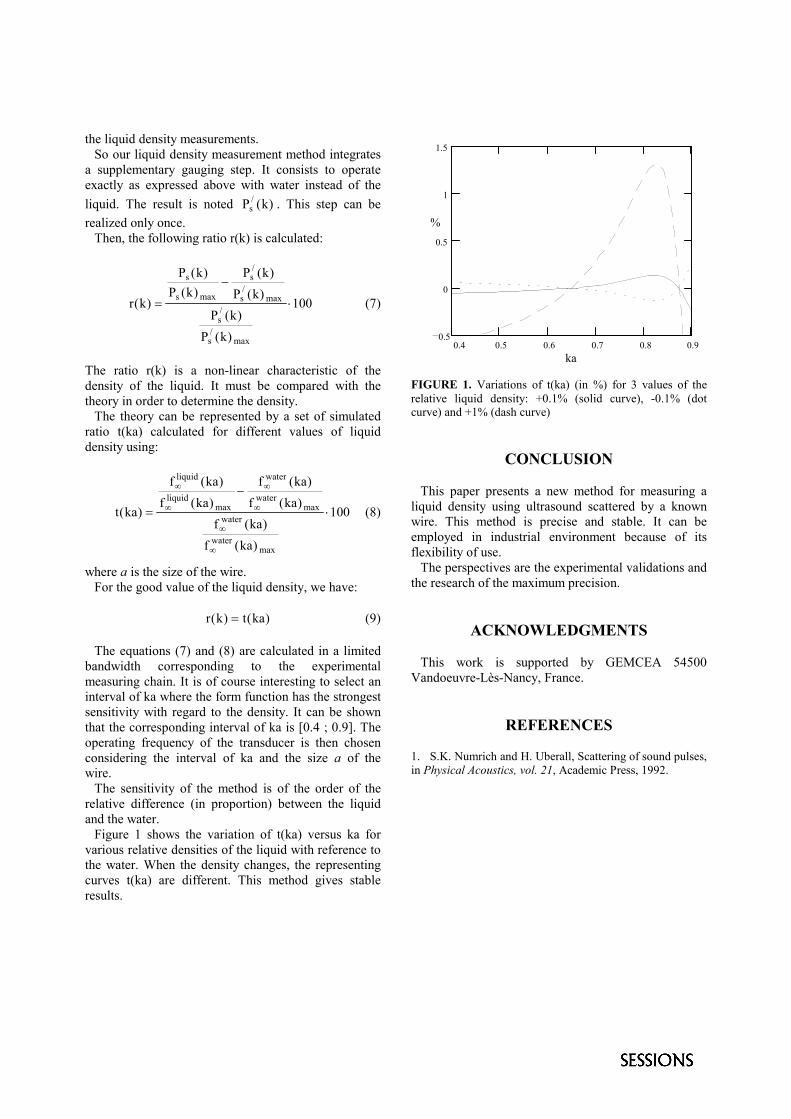
Figure 1 shows the variation of t(ka) versus ka for various relative densities of the liquid with reference to the water. When the density changes, the representing curves t(ka) are different. This method gives stable results.

0.4 0.5 0.6 0.7 0.8 0.90.5

0

0.5

1

1.5

FIGURE 1. Variations of t(ka) (in %) for 3 values of the relative liquid density: +0.1% (solid curve), -0.1% (dot curve) and +1% (dash curve)

CONCLUSION

This paper presents a new method for measuring a liquid density using ultrasound scattered by a known wire. This method is precise and stable. It can be employed in industrial environment because of its flexibility of use.

The perspectives are the experimental validations and the research of the maximum precision.

ACKNOWLEDGMENTS

This work is supported by GEMCEA 54500 Vandoeuvre-Lès-Nancy, France.

REFERENCES 1. S.K. Numrich and H. Uberall, Scattering of sound pulses, in Physical Acoustics, vol. 21, Academic Press, 1992.

ka

%

Accurate measurements of thermodynamic and transport properties of industrial gases with acoustic resonators

K. A. Gillis, J. J. Hurly, and M. R. Moldover

Process Measurements Division, National Institute of Standards and Technology, 20899 Gaithersburg, MD, USA

Acoustic resonators have been developed at NIST as tools to measure the thermodynamic and transport properties of gases. High Q cylindrical acoustic resonators are routinely used to measure the speed of sound in gases with uncertainties of 0.01% or less. Model intermolecular potentials are fitted to the acoustic data to obtain virial coefficients, gas densities ρ? and heat capacities CP with uncertainties of 0.1% as well as estimates of the viscosity η and thermal conductivity λ with uncertainties of less than 10 %. The viscosity is measured directly with uncertainties of less than 1 % using the Greenspan acoustic viscometer, a novel acoustic resonator developed at NIST. A novel resonator is used to measure the Prandtl number (Pr = ηCP/λ) with uncertainties of about 2 %. This paper summarizes our work with these resonators and their applications to numerous gases including very reactive gases used in semiconductor processing.

OVERVIEW

The National Institute of Standards and Technology (NIST) has an on-going research program to obtain accurate thermodynamic and transport property data of industrial gases. The gases that we study include ones that may be toxic, corrosive, reactive, flammable, or unstable at high temperature. We have studied more than 20 gases including refrigerants, chlorine, boron trichloride, tungsten hexafluoride, hydrogen bromide, carbon monoxide, and carbon tetrafluoride. These data are part of the Database of the Thermophysical Properties of Gases Used in the Semiconductor Industry accessible over the web at http://properties.nist.gov/SemiProp/. The success of this program has required the development of special gas-filled resonators and dosing systems to overcome the difficulties associated with the measurement and safe handling of these gases.

In order to obtain the desired data, this work exploits fundamental relationships between the acoustic and thermodynamic properties of gases through the use of high precision acoustic resonators [1]. We measure the frequency response of the resonators and its dependence on temperature and pressure. The results are analyzed with detailed acoustic models of gas-filled resonators, together with a calibration with argon.

In practice, the high precision of this technique is overshadowed by the uncertainty in the gas composition. This uncertainty is due to the presence of unknown impurities in the commercial sample and/or impurities that are generated during the scope of the study. Impurities of the latter type are

particularly troublesome because their concentration may change with time and the rate of change may depend on the temperature. Therefore, materials compatibility is a primary consideration. For this work, we have constructed acoustic resonators and gas handling systems in which stainless steel or Monel and gold are the only materials that the test gas touches [2].

With a low loss (high Q) cylindrical resonator, we obtain speed of sound, heat capacity, and density data over a wide range of temperature and pressure. The uncertainties in these data are typically ±0.01% for speed of sound, ±0.1% for the ideal gas heat capacity, and ±0.1% for the density. For some gases, we can also measure the average relaxation time of internal degrees of freedom [1].

Two other resonators developed in this program have geometries that are optimized for measuring the transport properties of gases. These “lossy” resonators exhibit greater thermal and viscous damping making them more suitable for accurately measuring the viscous or thermal diffusivity. The Greenspan acoustic viscometer [3] is a double Helmholtz resonator with which we have measured gas viscosity with a root-mean-squared (RMS) uncertainty of less than 0.5%. The other resonator is used for measurements of the Prandtl number, which is the ratio of the viscous and thermal diffusivities, with an uncertainty of about 2% [1].

RESONATOR DESIGNS

For our measurements of thermodynamic properties, we use a cylindrical resonator (65 mm

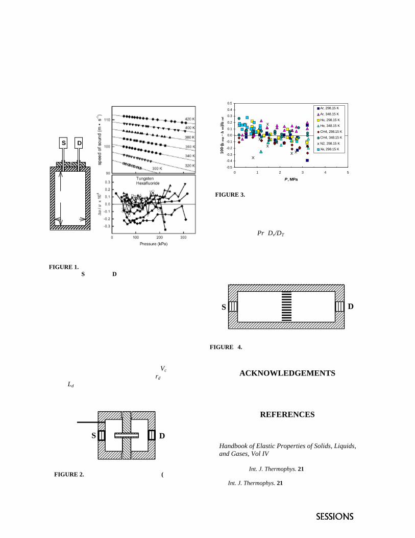
diameter and 140 mm length), as shown in Fig. 1 [2]. Sound is transmitted between the resonator and two remote electro-acoustic transducers (near room temperature) through argon-filled waveguides. Thin diaphragms transmit the sound between the test gas

and the pressure-balanced argon in the waveguides. Thus, the test gas never contacts the elastomers and other non-metal parts of the transducers. Also shown in Fig. 1 are the measured sound speeds in tungsten hexafluoride (WF6) and the deviations from a surface fit [2].

The Greenspan acoustic viscometer (shown in Fig. 2) is a double Helmholtz resonator formed by two identical chambers with volume Vc,(29 cm3) connected by a small duct of radius rd (2 mm) and length Ld.(31 mm). Again, the transducers are isolated from the test gas by thin diaphragms.

Figure 3 shows a comparison of the viscosity measured using the Greenspan viscometer with high quality data from the literature. These measurements have an RMS scatter of about 0.18% [3].

A third resonator (shown in Fig. 4) is designed for Prandtl number Pr=Dv/DT measurements [1]. This is a cylindrical resonator containing an array of ducts in the center region. Odd numbered longitudinal modes are damped primarily by viscous drag in the ducts and even numbered modes are damped primarily by thermal conduction to the duct walls.

ACKNOWLEDGEMENTS

This work was supported, in part, by the U.S. Office of Naval Research.

REFERENCES

1. Moldover, M.R., Gillis, K.A., Hurly, J.J., Mehl, J.B., Wilhelm, J. “Acoustic Measurements in Gases,” in Handbook of Elastic Properties of Solids, Liquids, and Gases, Vol IV, edited by Levy, Academic Press, San Diego, 2000, Ch. 12.

2. Hurly, J.,J., Int. J. Thermophys. 21, 185-206 (2000). 3. Wilhelm, J., Gillis, K.A., Mehl, J.B., and Moldover, M.

R., Int. J. Thermophys. 21, 983-996 (2000).

FIGURE 1. (a) The cylindrical resonator with remote transducers (Source and Detector). (b) Measured speed of sound in WF6 (upper) and deviations from a surface fit (lower) [2].

S D

65 mm

140 mm

(a) (b)

-0.5

-0.4

-0.3

-0.2

-0.1

0.0

0.1

0.2

0.3

0.4

0.5

0 1 2 3 4 5

P, MPa

10

0·(

ηexp

- η

ref)

/ ηre

f

Ar, 298.15 K

Ar, 348.15 K

He, 298.15 K

He, 348.15 K

CH4, 298.15 K

CH4, 348.15 K

N2, 298.15 K

Xe, 298.15 K

FIGURE 3. Deviations of the measured viscosity of several gases from known values. RMS deviations for all the data are about 0.18%.

FIGURE 2. A double Helmholtz resonator (Greenspan acoustic viscometer) used for viscosity measurements.

S D

FIGURE 4. A resonator designed for Prandtl number measurements.

S D

Time-frequency Analysis of Ultrasonic Backscattering Noisein Nondestructive Testing of Materials

J.V. Fuenteb, L.Vergaraa, J.Gosálbeza , R.Mirallesa,aETSI Telecomunicación , Univesidad Politécnica de Valencia,Camino de Vera s/n, 46022 Valencia, EspañabInstituto Tecnológico de la Construcción (AIDICO), Parc Tecnològic,46980, Paterna, Valencia, España

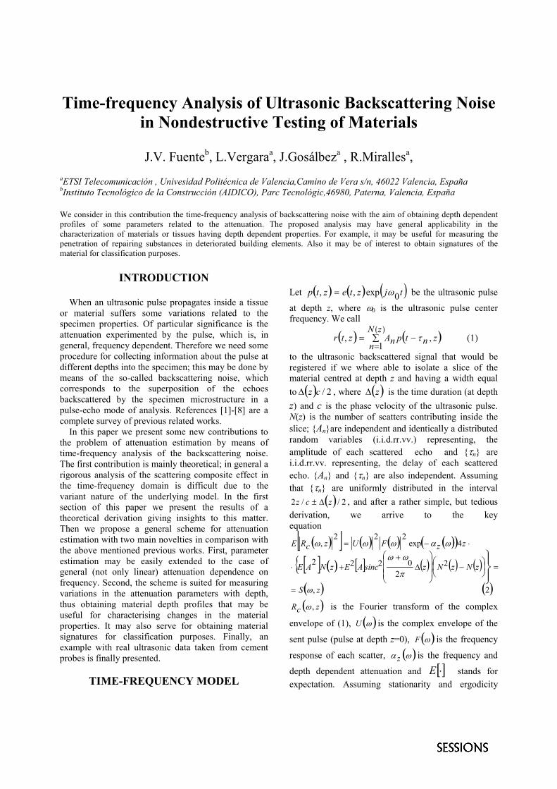
We consider in this contribution the time-frequency analysis of backscattering noise with the aim of obtaining depth dependentprofiles of some parameters related to the attenuation. The proposed analysis may have general applicability in thecharacterization of materials or tissues having depth dependent properties. For example, it may be useful for measuring thepenetration of repairing substances in deteriorated building elements. Also it may be of interest to obtain signatures of thematerial for classification purposes.

INTRODUCTION

When an ultrasonic pulse propagates inside a tissueor material suffers some variations related to thespecimen properties. Of particular significance is theattenuation experimented by the pulse, which is, ingeneral, frequency dependent. Therefore we need someprocedure for collecting information about the pulse atdifferent depths into the specimen; this may be done bymeans of the so-called backscattering noise, whichcorresponds to the superposition of the echoesbackscattered by the specimen microstructure in apulse-echo mode of analysis. References [1]-[8] are acomplete survey of previous related works. In this paper we present some new contributions tothe problem of attenuation estimation by means oftime-frequency analysis of the backscattering noise.The first contribution is mainly theoretical; in general arigorous analysis of the scattering composite effect inthe time-frequency domain is difficult due to thevariant nature of the underlying model. In the firstsection of this paper we present the results of atheoretical derivation giving insights to this matter.Then we propose a general scheme for attenuationestimation with two main novelties in comparison withthe above mentioned previous works. First, parameterestimation may be easily extended to the case ofgeneral (not only linear) attenuation dependence onfrequency. Second, the scheme is suited for measuringvariations in the attenuation parameters with depth,thus obtaining material depth profiles that may beuseful for characterising changes in the materialproperties. It may also serve for obtaining materialsignatures for classification purposes. Finally, anexample with real ultrasonic data taken from cementprobes is finally presented.

TIME-FREQUENCY MODEL

Let � � � � � �tjzteztp 0exp,, �� be the ultrasonic pulse

at depth z, where �0 is the ultrasonic pulse centerfrequency. We call

� �� �

� �zntpzN

n nAztr ,1

, ����

� (1)

to the ultrasonic backscattered signal that would beregistered if we where able to isolate a slice of thematerial centred at depth z and having a width equalto � � 2/cz� , where � �z� is the time duration (at depthz) and c is the phase velocity of the ultrasonic pulse.N(z) is the number of scatters contributing inside theslice; {An}are independent and identically a distributedrandom variables (i.i.d.rr.vv.) representing, theamplitude of each scattered echo and {�n} arei.i.d.rr.vv. representing, the delay of each scatteredecho. {An} and {�n} are also independent. Assumingthat {�n} are uniformly distributed in the interval

� � 2//2 zcz �� , and after a rather simple, but tediousderivation, we arrive to the keyequation

� �� � � � � � � �� �

� � � �� � � � � � � � �

� � � �2,

22

0222

4exp222

,

zS

zNzNzsincAEzNAE

zzFUzcRE

�

�

��

�����

�

���

���

��

���

�

�

���

�

�

�

���

��

���

� �zcR ,� is the Fourier transform of the complex

envelope of (1), � ��U is the complex envelope of the

sent pulse (pulse at depth z=0), � ��F is the frequency

response of each scatter, � ��� z is the frequency and

depth dependent attenuation and � ��E stands forexpectation. Assuming stationarity and ergodicity

along the analysis moving window duration, it can beverified that by means of computing quadratic time-frequency distributions (for example the spectrogram)of the actual register of backscattering noise, we mayobtain estimates of � �zS ,� . On the other hand wemay write

� �� � � � � �zLzzz

zS ,4,,log ���� ��� (3)

Then , depending on the particular application, we maydevise different procedures for estimating � ��� z from

estimates of � �zS ,� . A general scheme is proposed inthe next section.

PROPOSED SCHEME

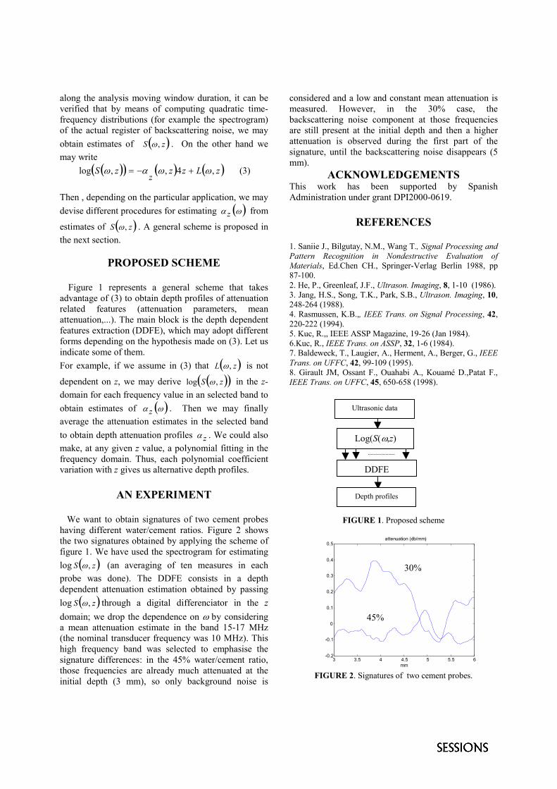
Figure 1 represents a general scheme that takesadvantage of (3) to obtain depth profiles of attenuationrelated features (attenuation parameters, meanattenuation,...). The main block is the depth dependentfeatures extraction (DDFE), which may adopt differentforms depending on the hypothesis made on (3). Let usindicate some of them.For example, if we assume in (3) that � �zL ,� is not

dependent on z, we may derive � �� �zS ,log � in the z-domain for each frequency value in an selected band toobtain estimates of � ��� z . Then we may finallyaverage the attenuation estimates in the selected bandto obtain depth attenuation profiles z� . We could alsomake, at any given z value, a polynomial fitting in thefrequency domain. Thus, each polynomial coefficientvariation with z gives us alternative depth profiles.

AN EXPERIMENT

We want to obtain signatures of two cement probeshaving different water/cement ratios. Figure 2 showsthe two signatures obtained by applying the scheme offigure 1. We have used the spectrogram for estimatinglog � �zS ,� (an averaging of ten measures in eachprobe was done). The DDFE consists in a depthdependent attenuation estimation obtained by passinglog � �zS ,� through a digital differenciator in the zdomain; we drop the dependence on � by consideringa mean attenuation estimate in the band 15-17 MHz(the nominal transducer frequency was 10 MHz). Thishigh frequency band was selected to emphasise thesignature differences: in the 45% water/cement ratio,those frequencies are already much attenuated at theinitial depth (3 mm), so only background noise is

considered and a low and constant mean attenuation ismeasured. However, in the 30% case, thebackscattering noise component at those frequenciesare still present at the initial depth and then a higherattenuation is observed during the first part of thesignature, until the backscattering noise disappears (5mm).

ACKNOWLEDGEMENTSThis work has been supported by SpanishAdministration under grant DPI2000-0619.

REFERENCES

1. Saniie J., Bilgutay, N.M., Wang T., Signal Processing andPattern Recognition in Nondestructive Evaluation ofMaterials, Ed.Chen CH., Springer-Verlag Berlin 1988, pp87-100.2. He, P., Greenleaf, J.F., Ultrason. Imaging, 8, 1-10 (1986).3. Jang, H.S., Song, T.K., Park, S.B., Ultrason. Imaging, 10,248-264 (1988).4. Rasmussen, K.B.,, IEEE Trans. on Signal Processing, 42,220-222 (1994).5. Kuc, R.,, IEEE ASSP Magazine, 19-26 (Jan 1984).6.Kuc, R., IEEE Trans. on ASSP, 32, 1-6 (1984).7. Baldeweck, T., Laugier, A., Herment, A., Berger, G., IEEETrans. on UFFC, 42, 99-109 (1995).8. Girault JM, Ossant F., Ouahabi A., Kouamé D.,Patat F.,IEEE Trans. on UFFC, 45, 650-658 (1998).

FIGURE 1. Proposed scheme

FIGURE 2. Signatures of two cement probes.

Log(S(�,z)

DDFE

Ultrasonic data

Depth profiles

3 3.5 4 4.5 5 5.5 6-0.2

-0.1

0

0.1

0.2

0.3

0.4

0.5

mm

attenuation (db/mm)

30%

45%

A novel test object for quantifying accuracy of smallvolumes scanned with 3D-ultrasound equipment

Chr. Kollmann and H. Bergmanna a,b

Department of Biomedical Engineering & Physics, University of Vienna, Waehringer Guertel 18-20,a

A-1090 Vienna, E-mail : ch.kollmann@bmtp.akh-wien.ac.at Ludwig-Boltzmann-Institute for Nuclear Medicine, Viennab

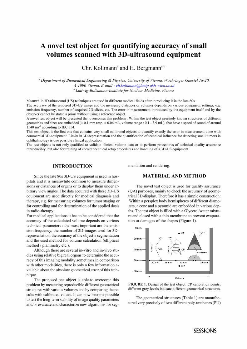
Meanwhile 3D-ultrasound (US) techniques are used in different medical fields after introducing it in the late 80s. The accuracy of the rendered 3D-US image and the measured distances or volumes depends on various equipment settings, e.g.emission frequency, number of acquired 2D-slices, etc. The error in measurement introduced by the equipment itself and by theobserver cannot be stated a priori without using a reference object.A novel test object will be presented that overcomes this problem : Within the test object precisely known structures of differentgeometries and sizes are embedded (± 0.1 mm resp. ± 0.06 mL, volume range : 0.1 - 3.9 mL), that have a speed of sound of around1540 ms according to IEC 854.-1

This test object is the first one that contains very small calibrated objects to quantify exactly the error in measurement done withcommercial 3D-equipment. Limits in 3D-representation and the quantification of technical influence for detecting small tumors inophthalmology is one possible clinical application.The test objects is not only qualified to validate clinical volume data or to perform procedures of technical quality assurancereproducibly, but also for training of correct technical setup procedures and handling of a 3D-US equipment.

INTRODUCTION

Since the late 80s 3D-US equipment is used in hos-pitals and it is meanwhile common to measure dimen-sions or distances of organs or to display them under ar- The novel test object is used for quality assurancebitrary view angles. The data acquired with these 3D-US (QA) purposes, mainly to check the accuracy of geome-equipment are used directly for medical diagnosis and trical 3D-display. Therefore it has a simple construction:therapy, e.g. for measuring volumes for tumor staging or Within a persplex body hemispheres of different diame-for controlling and for determination of the applied dosis ters, a cone and a pyramid are embedded in various dep-in radio-therapy. ths. The test object is filled with a Glycerol/water mixtu-For medical applications it has to be considered that the re and closed with a thin membrane to prevent evapora-accuracy of the calculated volume depends on various tion or damages of the shapes (Figure 1).technical parameters : the most important are the emis-sion frequency, the number of 2D-images used for 3D-representation, the accuracy of the object´s segmentationand the used method for volume calculation (ellipticalmethod / planimetry etc.).

Although there are several in-vitro and in-vivo stu-dies using relative big real organs to determine the accu-racy of this imaging modality sometimes in comparisonwith other modalities, there is only a few information a-vailable about the absolute geometrical error of this tech-nique.

The proposed test object is able to overcome thisproblem by measuring reproducible different geometricalstructures with various volumes and by comparing the re-sults with calibrated values. It can now become possibleto test the long-term stability of image quality parametersand/or evaluate and characterize new algorithms for seg-

mentation and rendering.

MATERIAL AND METHOD

FIGURE 1. Design of the test object. CP calibration points;different grey-levels indicate different geometrical structures.

The geometrical structures (Table 1) are manufac-tured very precisely of two different poly-urethanes (PU)

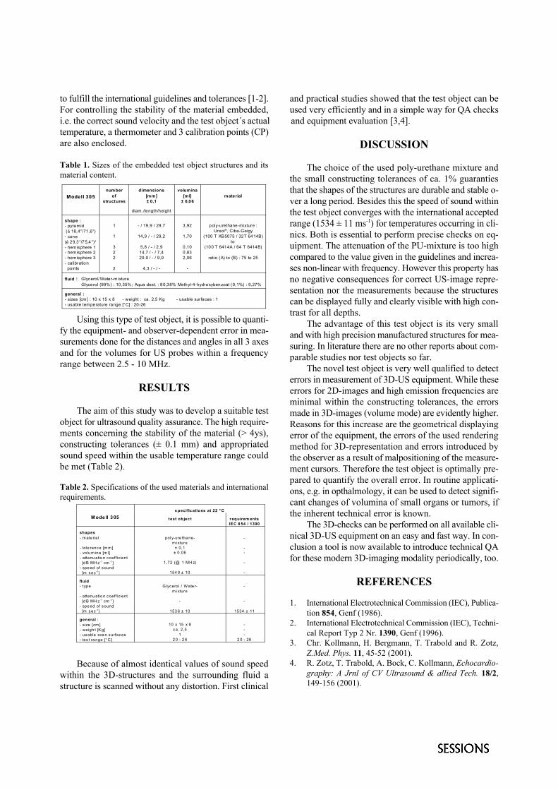
Modell 305number

ofstructures

dimensions[mm]± 0,1

volumina[ml]

± 0,06material

diam./length/height

shape :- pyramid (Ê18,4°/71,6°)- cone(Ê29,3°/75,4°)*- hemisphere 1- hemisphere 2- hemisphere 3- calibration points

1

1

322

2

- / 19,9 / 29,7

14,9 / - / 29,2

5,8 / - / 2,914,7 / - / 7 ,420.0 / - / 9 ,9

4,3 / - / -

3 ,92

1,70

0,100,832,06

-

poly-u rethane-mixture :Ureol®, Ciba-Geigy

(100 T XB5075 / 32T 6414B)to

(100 T 6414A / 64 T 6414B)

ratio (A) to (B) : 75 to 25

fluid : Glycerol/ Water-mixture Glycerol (99%) : 10,35%; Aqua dest. : 80,38% Methyl-4-hydroxybenzoat (0,1%) : 9,27%

general :- sizes [cm] : 10 x 15 x 8 - weight : ca . 2,5 Kg - usable surfaces : 1- usable temperature range [°C] : 20-26

M ode ll 3 05s pecific ations at 22 ° C

test objec t r equirem entsIE C 8 54 / 1390

shapes- m ate rial

- tole rance [m m ]- volu m ina [m l]- attenu atio n coeff icient [d B MH z-1 cm -1]- spe ed of sound [m sec-1]

pol y-ure tha ne-m i xture

± 0,1± 0 ,06

1,72 (@ 1 MH z)

154 0 ± 10

-

--

-

-

fluid- type

- attenu atio n coeff icient [d B MH z-1 cm -1]- spe ed of sound [m sec-1]

G lycerol / W ate r-m i xture

-

153 6 ± 10

-

-

1534 ± 11

general :- size [cm ]- weigh t [K g]- usable sca n surfaces- tes t ra nge [° C]

10 x 15 x 8ca. 2,5

12 0 - 2 6

---

2 0 - 26

to fulfill the international guidelines and tolerances [1-2]. and practical studies showed that the test object can beFor controlling the stability of the material embedded, used very efficiently and in a simple way for QA checksi.e. the correct sound velocity and the test object´s actual and equipment evaluation [3,4].temperature, a thermometer and 3 calibration points (CP)are also enclosed.

Table 1. Sizes of the embedded test object structures and itsmaterial content.

Using this type of test object, it is possible to quanti-fy the equipment- and observer-dependent error in mea-surements done for the distances and angles in all 3 axesand for the volumes for US probes within a frequencyrange between 2.5 - 10 MHz.

RESULTS

The aim of this study was to develop a suitable testobject for ultrasound quality assurance. The high require-ments concerning the stability of the material (> 4ys),constructing tolerances (± 0.1 mm) and appropriatedsound speed within the usable temperature range couldbe met (Table 2).

Table 2. Specifications of the used materials and internationalrequirements.

Because of almost identical values of sound speedwithin the 3D-structures and the surrounding fluid astructure is scanned without any distortion. First clinical

DISCUSSION

The choice of the used poly-urethane mixture andthe small constructing tolerances of ca. 1% guarantiesthat the shapes of the structures are durable and stable o-ver a long period. Besides this the speed of sound withinthe test object converges with the international acceptedrange (1534 ± 11 ms ) for temperatures occurring in cli--1

nics. Both is essential to perform precise checks on eq-uipment. The attenuation of the PU-mixture is too highcompared to the value given in the guidelines and increa-ses non-linear with frequency. However this property hasno negative consequences for correct US-image repre-sentation nor the measurements because the structurescan be displayed fully and clearly visible with high con-trast for all depths.

The advantage of this test object is its very smalland with high precision manufactured structures for mea-suring. In literature there are no other reports about com-parable studies nor test objects so far.

The novel test object is very well qualified to detecterrors in measurement of 3D-US equipment. While theseerrors for 2D-images and high emission frequencies areminimal within the constructing tolerances, the errorsmade in 3D-images (volume mode) are evidently higher.Reasons for this increase are the geometrical displayingerror of the equipment, the errors of the used renderingmethod for 3D-representation and errors introduced bythe observer as a result of malpositioning of the measure-ment cursors. Therefore the test object is optimally pre-pared to quantify the overall error. In routine applicati-ons, e.g. in opthalmology, it can be used to detect signifi-cant changes of volumina of small organs or tumors, ifthe inherent technical error is known.

The 3D-checks can be performed on all available cli-nical 3D-US equipment on an easy and fast way. In con-clusion a tool is now available to introduce technical QAfor these modern 3D-imaging modality periodically, too.

REFERENCES

1. International Electrotechnical Commission (IEC), Publica-tion 854, Genf (1986).

2. International Electrotechnical Commission (IEC), Techni-cal Report Typ 2 Nr. 1390, Genf (1996).

3. Chr. Kollmann, H. Bergmann, T. Trabold and R. Zotz,Z.Med. Phys. 11, 45-52 (2001).

4. R. Zotz, T. Trabold, A. Bock, C. Kollmann, Echocardio-graphy: A Jrnl of CV Ultrasound & allied Tech. 18/2,149-156 (2001).

Properties of Acoustic Emission Signals for Tool ConditionMonitoring (TCM) Applications

G.Pontuale, F.A.Farrelly, A.Petri, L.Pitolli, F.Krogh

Istituto di Acustica "O.M.Corbino", Consiglio Nazionale delle Ricerche, 00133 Rome, Italye-mail pontuale@idac.rm.cnr.it

AbstractAcoustic Emission data from mechanical machining with carbide cutting tools are analyzed, so as to reach a deeperunderstanding of the signal properties for Tool Condition Monitoring applications. They are gathered with a custom-builttransducer capable of collecting signals close to the working point, thus allowing us to perform acquisitions in favorableconditions. By statistical analysis of the time series data and RMS values at various tool wear levels, we find that ageing featurescan be put into evidence in all cases. In particular, the histograms of raw data show that their distribution is power-law above across-over value, with larger events being more numerous in newer cutting tools when compared to more worn-out ones. Forpractical purposes, statistics based on root mean square values are more convenient, and are also capable of discriminatingbetween tool wear levels. The assumption that experimental RMS histograms follow a Beta distribution has been tested, leadingto the observation that direct comparison of the fitting Beta curves with experimental data shows relevant discrepancies, makingthe search of a more appropriate fitting function for the experimental distribution desiderable.

INTRODUCTION

The challenge of extensively using TCM devices andtechniques in industrial manufacturing process hasbecome ever more important. In this field, a continuousimprovement in terms of reliability and practicality ofsensor systems is mandatory, in order to reach thegoals of product quality improvements, reduced non-productive times and thus considerable costs savings.Acoustic Emission (AE) signal analysis has beendemonstrated to be one of the most efficient TCMtechniques which can be applied to machiningprocesses control, as the impressive amount ofliterature on this subject shows [1].

ACOUSTIC EMISSION SIGNAL

Internally generated stress waves, liberated duringdynamic processes in solid materials, can result insudden irreversible release of elastic waves generallycalled Acoustic Emission (AE). In the present case theprincipal sources of these signals can be attributed tosurface deformations (and possibly below the surface)as well as to detachments that take place at the

FIGURE 1. Time series illustrating both continuous AEcomponents and burst AE events.

interface between the machined sample and the worktool. In the analysis of AE signals generated duringtool machining processes, two rather well distinct partscan be identified: a continuous emission and the burstemission exhibiting strong intermittence, and relativelyhigh amplitudes. These AE signal features are wellshown in the time splice of Fig.1.

OPERATIONAL CONDITION ANDEXPERIMENTAL RESULTS

In all measurements, cutting tool inserts are''IMPERO'' PCLNR with 2020/12 type tungstencarbide; the acquisitions have been performed oninserts with three different degrees of wear: new ones,those estimated to be half-way through their life-cycle(50%) and those completely worn through (100%). TheAE transducer used to collect signals is a smallrectangular shaped piezoelectric ceramic (PZT-5)housed inside a little cavity bored into the cutting toolholder such as to protect it from chip damages or liquidcoolant effects, and placed very close to the cuttingtool insert itself in order to limit signal attenuations anddistortions of the propagating elastic wave. Thedetected signal is amplified and filtered in the 200kHz-1MHz range, is then captured by a Tektronixdigital oscilloscope (TDS420) using a 2.5 MHzsampling rate, and finally stored in a PC through anIEEE488 interface. The data has been analyzed bothdirectly in its time series form and through Root MeanSquared (RMS) values.The histograms of the absolute value of time seriesamplitudes taken from measurements performed using

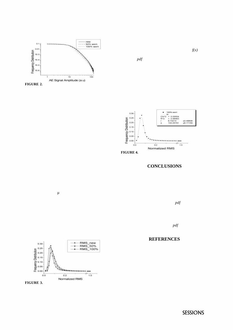
FIGURE 2. The histograms of the absolute values of theamplitude on log-log scale for the 3 levels of wear

inserts in three stages of wear, are portrayed in Fig. 2.The curves exhibit a power-law behavior above across-over value, with a similar slope for all threestages of wear. Furthermore, in this range, the dataderived from measurements using tools with greaterwear, show a smaller frequency count for a given valuein amplitude, this leads to the conclusion that in this setof trials the newer tools are the most active ones interms of acoustic emission. It is interesting to note thatthis power-law behavior has been observed in manystudies on acoustic emission signals, e.g. thoseassociated with the formation of microfractures [2],and is generally associated with scale invariantproperties underlying the physical phenomena understudy. In some cases this has been explained by SOC(Self-Organized Criticality) [3] models. Thesepromising results stimulate us into future investigatingon these AE power-law features correlated with toolwear. The analysis of the RMS has been conductedcalculating values on the basis of 100 points,corresponding to 40 µs. In Fig.3 the overall histogramsof the three families are compared, indicating anoticeable shift towards lower levels of the modalvalue of the frequency distribution for increasing levelsof wear, and a change in the skewness tending towardsvalues compatible with a symmetrical shape. Thisapproach seems to be effective in discriminating toolwear states and could be used as the basis forimplementing algorithms for TCM systems. Inliterature, borrowing from a technique used in the

FIGURE 3. The frequency distribution of RMS values forthe 3 levels of wear.

description of surfaces roughness [4], various attemptshave been made at determining tool condition relyingon the hypothesis that a beta distribution f(x) [5,6],properly describes the Probability DistributionFunction (pdf) of the RMS values. In Fig.4, the best-fitof the frequency distributions of one of the data-sets inFig.3 is shown. From these graphs we see that whilethere is a good matching between the fitting functionand the data sets in the neighborhood of the peaks,some discrepancies are found for RMS values justabove the peak where the curves level off; thisindicates that in this range, the data sets are richer inevents than what the Beta function would indicate.This suggests that a better empirical fitting-functionmay exist.

FIGURE 4. Best-fit of one of the frequency distributions inFig.3 with a Beta function.

CONCLUSIONS

We have seen that it is possible to obtain informationon tool wear conditions analyzing AE time series andRMS values, both capable of showing somediscriminating features. Interesting power-lawcharacteristics have been identified for the time series,through the use of log-log histograms. An often usedmodel for describing the RMS's pdf by way of theBeta distribution has been tested. The comparison ofthe experimental distributions with their Beta functionbest-fit shows a less than perfect matching between thetwo sets; future efforts will be dedicated to thetheoretical form of the RMS's pdf values related topower-law distributed time series.

REFERENCES

1. G.Byrne, D.Dornfeld, I.Inasaki, G.Ketteler, W.Konig andR.Teti, Annals of CIRP, 44-2, 541 (1995)

2. A.Petri, Phil.Mag.B, 77-2, 491 (1998)3. P.Bak, C.Tang and K.Wiesenfeld, Phys.Rev.Lett. 59, 381

(1997)4. D.J.Whitehouse, annals of CIRP, 27, 491 (1978)5. E.Kannatey-Asibu and D.A.Dornfeld, Wear, 76, 247 (1982)6. K.Jemielniak and O.Otman, J.Mat.Proc.Tech. , 76, 192 (1998)

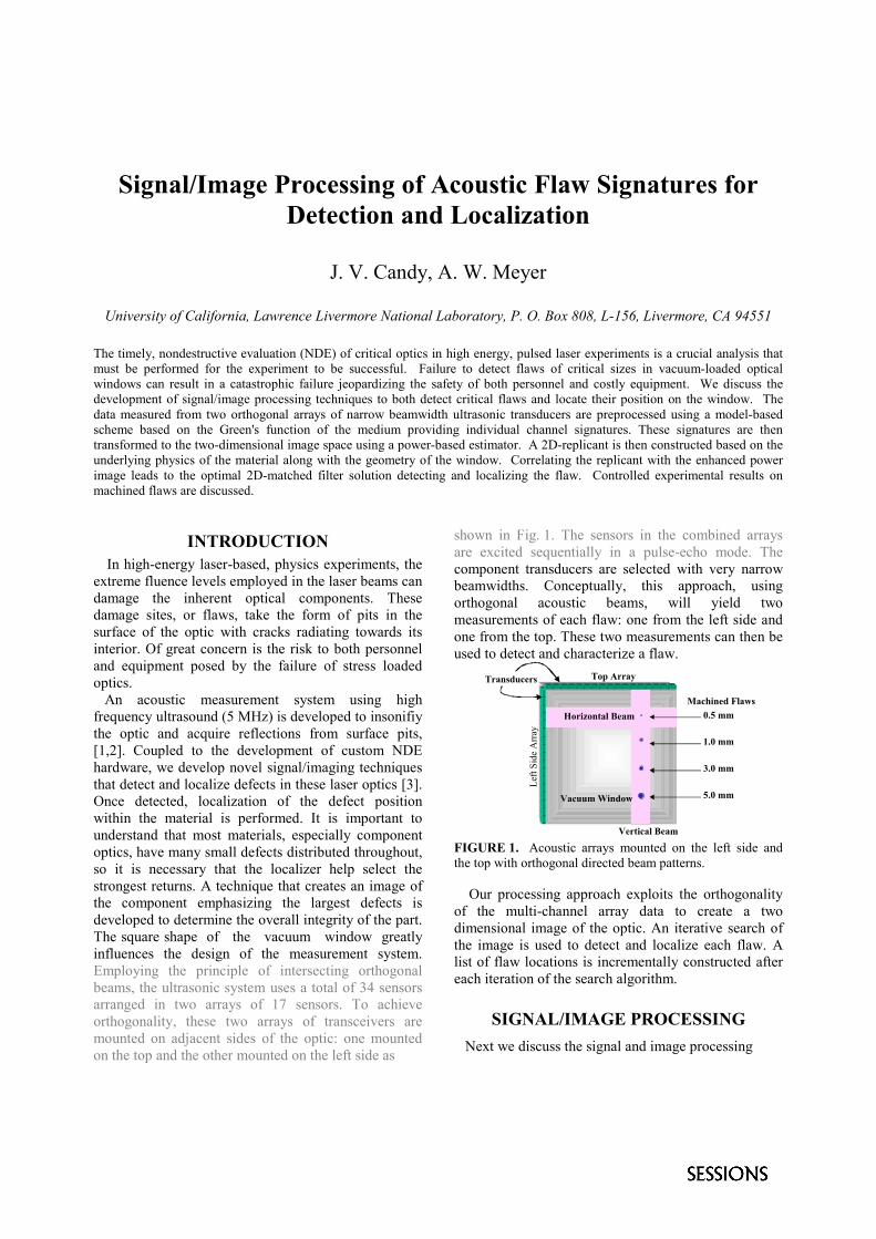
Signal/Image Processing of Acoustic Flaw Signatures forDetection and Localization

J. V. Candy, A. W. Meyer

University of California, Lawrence Livermore National Laboratory, P. O. Box 808, L-156, Livermore, CA 94551

The timely, nondestructive evaluation (NDE) of critical optics in high energy, pulsed laser experiments is a crucial analysis thatmust be performed for the experiment to be successful. Failure to detect flaws of critical sizes in vacuum-loaded opticalwindows can result in a catastrophic failure jeopardizing the safety of both personnel and costly equipment. We discuss thedevelopment of signal/image processing techniques to both detect critical flaws and locate their position on the window. Thedata measured from two orthogonal arrays of narrow beamwidth ultrasonic transducers are preprocessed using a model-basedscheme based on the Green's function of the medium providing individual channel signatures. These signatures are thentransformed to the two-dimensional image space using a power-based estimator. A 2D-replicant is then constructed based on theunderlying physics of the material along with the geometry of the window. Correlating the replicant with the enhanced powerimage leads to the optimal 2D-matched filter solution detecting and localizing the flaw. Controlled experimental results onmachined flaws are discussed.

INTRODUCTION In high-energy laser-based, physics experiments, theextreme fluence levels employed in the laser beams candamage the inherent optical components. Thesedamage sites, or flaws, take the form of pits in thesurface of the optic with cracks radiating towards itsinterior. Of great concern is the risk to both personneland equipment posed by the failure of stress loadedoptics. An acoustic measurement system using highfrequency ultrasound (5 MHz) is developed to insonifiythe optic and acquire reflections from surface pits,[1,2]. Coupled to the development of custom NDEhardware, we develop novel signal/imaging techniquesthat detect and localize defects in these laser optics [3].Once detected, localization of the defect positionwithin the material is performed. It is important tounderstand that most materials, especially componentoptics, have many small defects distributed throughout,so it is necessary that the localizer help select thestrongest returns. A technique that creates an image ofthe component emphasizing the largest defects isdeveloped to determine the overall integrity of the part.The square shape of the vacuum window greatlyinfluences the design of the measurement system.Employing the principle of intersecting orthogonalbeams, the ultrasonic system uses a total of 34 sensorsarranged in two arrays of 17 sensors. To achieveorthogonality, these two arrays of transceivers aremounted on adjacent sides of the optic: one mountedon the top and the other mounted on the left side as

shown in Fig. 1. The sensors in the combined arraysare excited sequentially in a pulse-echo mode. Thecomponent transducers are selected with very narrowbeamwidths. Conceptually, this approach, usingorthogonal acoustic beams, will yield twomeasurements of each flaw: one from the left side andone from the top. These two measurements can then beused to detect and characterize a flaw.

Machined Flaws0.5 mm

1.0 mm

3.0 mm

5.0 mm

Top Array

Left

Side

Arra

y

Horizontal Beam

Vertical Beam

Transducers

Vacuum Window

FIGURE 1. Acoustic arrays mounted on the left side andthe top with orthogonal directed beam patterns.

Our processing approach exploits the orthogonalityof the multi-channel array data to create a twodimensional image of the optic. An iterative search ofthe image is used to detect and localize each flaw. Alist of flaw locations is incrementally constructed aftereach iteration of the search algorithm.

SIGNAL/IMAGE PROCESSING Next we discuss the signal and image processing

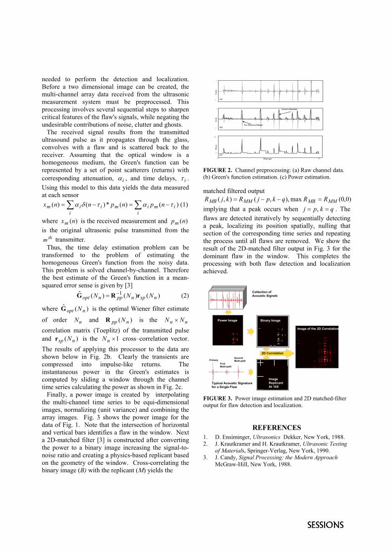
needed to perform the detection and localization.Before a two dimensional image can be created, themulti-channel array data received from the ultrasonicmeasurement system must be preprocessed. Thisprocessing involves several sequential steps to sharpencritical features of the flaw's signals, while negating theundesirable contributions of noise, clutter and ghosts. The received signal results from the transmittedultrasound pulse as it propagates through the glass,convolves with a flaw and is scattered back to thereceiver. Assuming that the optical window is ahomogeneous medium, the Green's function can berepresented by a set of point scatterers (returns) withcorresponding attenuation, i� , and time delays, i� .Using this model to this data yields the data measuredat each sensor

�� ����

iimim

iiim npnpnnx )()(*)()( ����� (1)

where )(nxm is the received measurement and )(npmis the original ultrasonic pulse transmitted from the

thm transmitter. Thus, the time delay estimation problem can betransformed to the problem of estimating thehomogeneous Green's function from the noisy data.This problem is solved channel-by-channel. Thereforethe best estimate of the Green's function in a mean-squared error sense is given by [3]

)()()(ˆ 1nxpnppnopt NNN rRG �

� (2)

where )(ˆnopt NG is the optimal Wiener filter estimate

of order nN and )( npp NR is the nn NN �

correlation matrix (Toeplitz) of the transmitted pulseand )( nxp Nr is the 1�nN cross–correlation vector.The results of applying this processor to the data areshown below in Fig. 2b. Clearly the transients arecompressed into impulse-like returns. Theinstantaneous power in the Green's estimates iscomputed by sliding a window through the channeltime series calculating the power as shown in Fig. 2c. Finally, a power image is created by interpolatingthe multi-channel time series to be equi-dimensionalimages, normalizing (unit variance) and combining thearray images. Fig. 3 shows the power image for thedata of Fig. 1. Note that the intersection of horizontaland vertical bars identifies a flaw in the window. Nexta 2D-matched filter [3] is constructed after convertingthe power to a binary image increasing the signal-to-noise ratio and creating a physics-based replicant basedon the geometry of the window. Cross-correlating thebinary image (B) with the replicant (M) yields the

Vol

tsV

olts

Wat

ts

(a)

(b)

(c)

Pre-Processed Signal

Green’s Function

1

-1

Time (µs)0 155

1

-1

5.5

0

FIGURE 2. Channel preprocessing: (a) Raw channel data.(b) Green's function estimation. (c) Power estimation.

matched filtered output)0,0(max ,),(),( MMMBMMMB RRqkpjRkjR ����

implying that a peak occurs when qkpj �� , . Theflaws are detected iteratively by sequentially detectinga peak, localizing its position spatially, nulling thatsection of the corresponding time series and repeatingthe process until all flaws are removed. We show theresult of the 2D-matched filter output in Fig. 3 for thedominant flaw in the window. This completes theprocessing with both flaw detection and localizationachieved.

PrimaryFirstMulti-path

SecondMulti-path

Typical Acoustic Signaturefor a Single Flaw

Collection ofAcoustic Signals

Power Image

10 20 30 40 50 60

ImageReplicantAt 10X

2D Correlation

Binary Image

Image of the 2D Correlation

FIGURE 3. Power image estimation and 2D matched-filteroutput for flaw detection and localization.

REFERENCES1. D. Ensiminger, Ultrasonics Dekker, New York, 1988.2. J. Krautkramer and H. Krautkramer, Ultrasonic Testing

of Materials, Springer-Verlag, New York, 1990.3. J. Candy, Signal Processing: the Modern Approach

McGraw-Hill, New York, 1988.

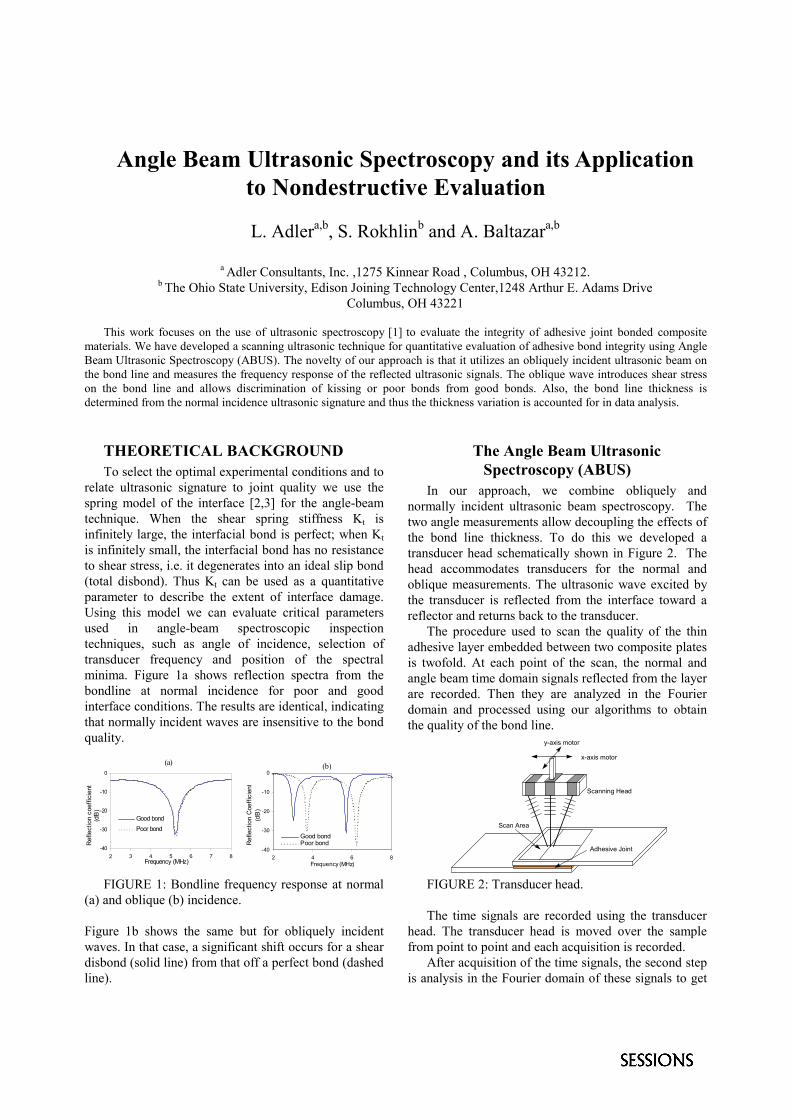
Angle Beam Ultrasonic Spectroscopy and its Applicationto Nondestructive Evaluation

L. Adlera,b, S. Rokhlinb and A. Baltazara,b

a Adler Consultants, Inc. ,1275 Kinnear Road , Columbus, OH 43212.b The Ohio State University, Edison Joining Technology Center,1248 Arthur E. Adams Drive

Columbus, OH 43221

This work focuses on the use of ultrasonic spectroscopy [1] to evaluate the integrity of adhesive joint bonded compositematerials. We have developed a scanning ultrasonic technique for quantitative evaluation of adhesive bond integrity using AngleBeam Ultrasonic Spectroscopy (ABUS). The novelty of our approach is that it utilizes an obliquely incident ultrasonic beam onthe bond line and measures the frequency response of the reflected ultrasonic signals. The oblique wave introduces shear stresson the bond line and allows discrimination of kissing or poor bonds from good bonds. Also, the bond line thickness isdetermined from the normal incidence ultrasonic signature and thus the thickness variation is accounted for in data analysis.

THEORETICAL BACKGROUNDTo select the optimal experimental conditions and to

relate ultrasonic signature to joint quality we use thespring model of the interface [2,3] for the angle-beamtechnique. When the shear spring stiffness Kt isinfinitely large, the interfacial bond is perfect; when Ktis infinitely small, the interfacial bond has no resistanceto shear stress, i.e. it degenerates into an ideal slip bond(total disbond). Thus Kt can be used as a quantitativeparameter to describe the extent of interface damage.Using this model we can evaluate critical parametersused in angle-beam spectroscopic inspectiontechniques, such as angle of incidence, selection oftransducer frequency and position of the spectralminima. Figure 1a shows reflection spectra from thebondline at normal incidence for poor and goodinterface conditions. The results are identical, indicatingthat normally incident waves are insensitive to the bondquality.

FIGURE 1: Bondline frequency response at normal(a) and oblique (b) incidence.

Figure 1b shows the same but for obliquely incidentwaves. In that case, a significant shift occurs for a sheardisbond (solid line) from that off a perfect bond (dashedline).

The Angle Beam UltrasonicSpectroscopy (ABUS)

In our approach, we combine obliquely andnormally incident ultrasonic beam spectroscopy. Thetwo angle measurements allow decoupling the effects ofthe bond line thickness. To do this we developed atransducer head schematically shown in Figure 2. Thehead accommodates transducers for the normal andoblique measurements. The ultrasonic wave excited bythe transducer is reflected from the interface toward areflector and returns back to the transducer.

The procedure used to scan the quality of the thinadhesive layer embedded between two composite platesis twofold. At each point of the scan, the normal andangle beam time domain signals reflected from the layerare recorded. Then they are analyzed in the Fourierdomain and processed using our algorithms to obtainthe quality of the bond line.

FIGURE 2: Transducer head.

The time signals are recorded using the transducerhead. The transducer head is moved over the samplefrom point to point and each acquisition is recorded.

After acquisition of the time signals, the second stepis analysis in the Fourier domain of these signals to get

(b)

-40

-30

-20

-10

0

2 4 6 8Frequency (MHz)

Refle

ctio

n C

oeffi

cien

t(d

B)

Good bondPoor bond

(a)

-40

-30

-20

-10

0

2 3 4 5 6 7 8Frequency (MHz)

Ref

lect

ion

coef

ficie

nt(d

B)

Good bondPoor bond

x-axis motor

y-axis motor

Scanning Head

Adhesive Joint

Scan Area

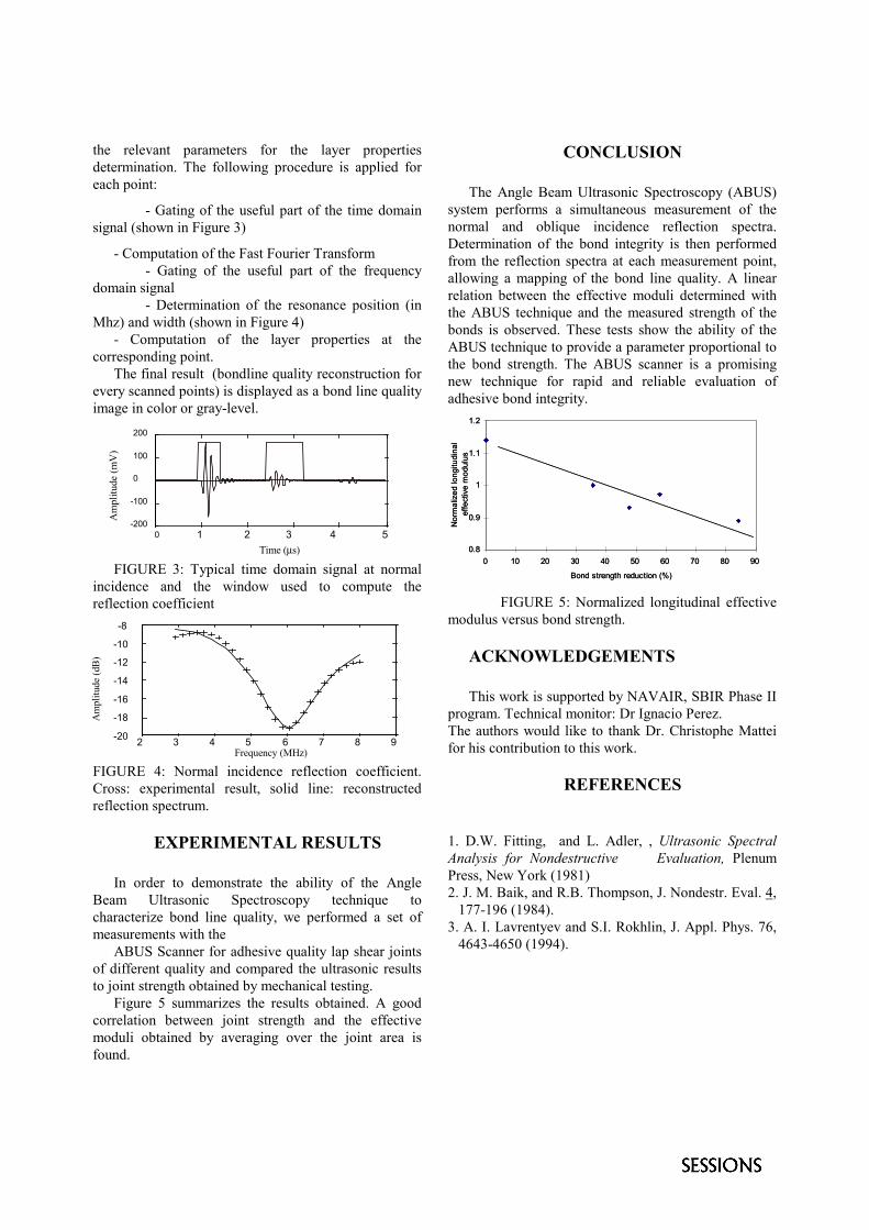
the relevant parameters for the layer propertiesdetermination. The following procedure is applied foreach point:

- Gating of the useful part of the time domainsignal (shown in Figure 3)

- Computation of the Fast Fourier Transform- Gating of the useful part of the frequency

domain signal- Determination of the resonance position (in

Mhz) and width (shown in Figure 4)- Computation of the layer properties at the

corresponding point.The final result (bondline quality reconstruction for

every scanned points) is displayed as a bond line qualityimage in color or gray-level.

FIGURE 3: Typical time domain signal at normalincidence and the window used to compute thereflection coefficient

FIGURE 4: Normal incidence reflection coefficient.Cross: experimental result, solid line: reconstructedreflection spectrum.

EXPERIMENTAL RESULTS

In order to demonstrate the ability of the AngleBeam Ultrasonic Spectroscopy technique tocharacterize bond line quality, we performed a set ofmeasurements with the

ABUS Scanner for adhesive quality lap shear jointsof different quality and compared the ultrasonic resultsto joint strength obtained by mechanical testing.

Figure 5 summarizes the results obtained. A goodcorrelation between joint strength and the effectivemoduli obtained by averaging over the joint area isfound.

CONCLUSION

The Angle Beam Ultrasonic Spectroscopy (ABUS)system performs a simultaneous measurement of thenormal and oblique incidence reflection spectra.Determination of the bond integrity is then performedfrom the reflection spectra at each measurement point,allowing a mapping of the bond line quality. A linearrelation between the effective moduli determined withthe ABUS technique and the measured strength of thebonds is observed. These tests show the ability of theABUS technique to provide a parameter proportional tothe bond strength. The ABUS scanner is a promisingnew technique for rapid and reliable evaluation ofadhesive bond integrity.

FIGURE 5: Normalized longitudinal effectivemodulus versus bond strength.

ACKNOWLEDGEMENTS

This work is supported by NAVAIR, SBIR Phase IIprogram. Technical monitor: Dr Ignacio Perez.The authors would like to thank Dr. Christophe Matteifor his contribution to this work.

REFERENCES

1. D.W. Fitting, and L. Adler, , Ultrasonic SpectralAnalysis for Nondestructive Evaluation, PlenumPress, New York (1981)2. J. M. Baik, and R.B. Thompson, J. Nondestr. Eval. 4,

177-196 (1984).3. A. I. Lavrentyev and S.I. Rokhlin, J. Appl. Phys. 76,

4643-4650 (1994).

2 3 4 5 6 7 8 9-20

-18

-16

-14

-12

-10

-8

Frequency (MHz)

Am

plitu

de (d

B)

0 1 2 3 4 5-200

-100

0

100

200

Am

plitu

de (m

V)

Time (µs) 0.8

0.9

1

1.1

1.2

0 10 20 30 40 50 60 70 80 90

Bond strength reduction (%)

Nor

mal

ized

long

itudi

nal

effe

ctiv

e m

odul

us

0.8

0.9

1

1.1

1.2

0 10 20 30 40 50 60 70 80 90

Bond strength reduction (%)

Nor

mal

ized

long

itudi

nal

effe

ctiv

e m

odul

us

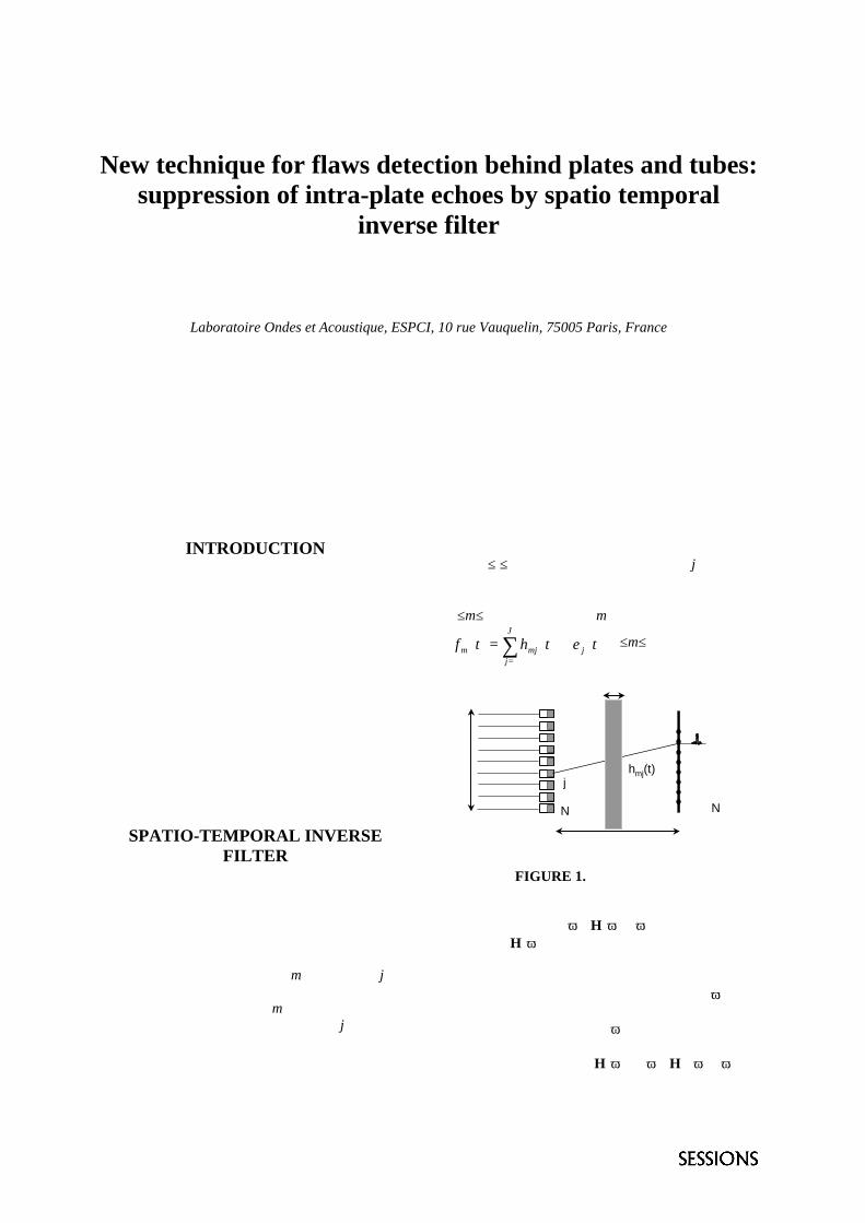
New technique for flaws detection behind plates and tubes:suppression of intra-plate echoes by spatio temporal

inverse filter

J.-F. Aubry, M. Tanter, J.-L. Thomas, and M. Fink

Laboratoire Ondes et Acoustique, ESPCI, 10 rue Vauquelin, 75005 Paris, France

It is very difficult to detect flaws behind plates, ribs or tubes, as the presence of multiple interfaces induces reflected wavefronts that follow the main wave front. Using a time reversal mirror could solve the problem by suppressing the echoes butwould require a complete cavity with transducers surrounding the sample, which is hard to achieve experimentally.We propose here a new focusing technique, called spatio-temporal inverse filter, based on the inversion of the propagationoperator at each frequency within the bandwidth of our transducers. We will show experimental results proving that it ispossible to suppress intra plate echoes by emitting a complex temporal shape with one array of transducers located outside thesample, improving the axial focusing. Effects of the transverse waves that are generated on the interfaces are alsocompensated. Moreover, we will see that the lateral resolution can be greatly enhanced by taking advantage of the geometry ofthe sample. In fact, this promising technique enables to reach the optimal focusing achievable by the focusing apparatus, for agiven aperture of the array and a given bandwidth of the transducers.

INTRODUCTION

Ultrasonic detection of defects behind plates, tubes,spars or ribs is very difficult to achieve because ofmultiple reflections that degrade the focusing. Weexploit here the great potential of a new focusingtechnique based on the inversion of the propagationoperator between the emitting plane characterized bythe emitting array of transducers and the focal plane.After a brief presentation of this technique, we willshow its results while focusing through a titaniumplate. Comparison between the focusing patternobtained with a cylindrical law and this technique willbe presented.

SPATIO-TEMPORAL INVERSEFILTER

A similar method had first been exposed in [1], and thewhole process is fully described in [2,3]. Basically, atitanium plate is placed between an array of piezoelectric transducers and a set of N control points(hydrophones) placed in the focal plane (Figure 1).For each couple (control point m, transducer j), wedefine the impulse response hmj(t), which correspondsto the signal received on the mth control point after atemporal Dirac function is applied on the jth transducerof the array. This response includes all the propagationeffects through the considered medium as well as the

acousto-electric responses of the two elements. Letej(t), 1≤j≤J, being the input signal on the jth transducer.As the transformations are supposed linear andinvariant under a time shift, the output signal fm(t),1≤m≤M, received on the mth control point is given by:

∑=

⊗=J

jjmjm tethtf

1

)()()( , 1≤m≤M.

FIGURE 1. Experimental setup.

A temporal Fourier transform leads in the matrixformalism to: F(ω)=H(ω)E(ω): the propagationoperator H(ω) describes the propagation in themedium from the array to the set of control points.In our case, as we want to focus through the plate, wehave to determine the field distribution E(ω) on thetransducer array that would give rise, after propagationto the field distribution F(ω) (F was chosen to be aspatio-temporal Dirac function) on the control plane.So that one has to invert H(ω): E(ω)=H-1(ω)F(ω).

1

m

j

N

1

N

hmj(t)

100mm

64m

m

Array of transducers Set of controlpoints

25mm

(Titanium)

water

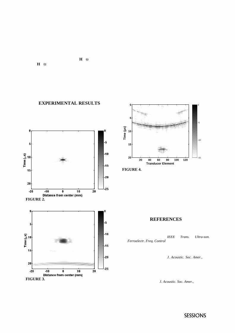
A pseudo-inversion is realized by means of a SingularValue Decomposition in which the physical signals areinverted while the signals below the noise sensitivityof our experimental setup are equated to zero, leadingto a noise-filtered approximation H-1(ω) of the inversematrix H-1(ω).This is performed at each frequency within thebandwidth of the transducer and the final signal toemit on the array of transducers is obtained after goingback to the time domain by inverse Fourier transform.

EXPERIMENTAL RESULTS

The B-scan presented in Fig.2 clearly shows that thefocusing pattern is degraded by intra-plate reflectionswhen using a cylindrical law.

FIGURE 2. B-scan through the plate (cylindrical law).

FIGURE 3. B-scan through the plate (inverse filter).

The B-scan presented in Fig.2 clearly shows that thefocusing pattern is degraded by intra-plate reflections

when using a cylindrical law: a reflected wave frontarrives 10µs after the principal wave front. Thepropagation operator H was then acquired andinverted, giving rise to inverse-filter-derived emissionvector {e(t)} presented on Fig. 4. The B-scan obtainedat focus is plotted on Fig.3: the plate echoes are clearlyremoved, thanks to a second wavefront emitted by thearray at time 17µs (Fig.4) that destructively interferewith the intraplate echoes of the main wavefront (attime 7µs on Fig.4). Moreover, the axial resolution ismuch better thanks to the use of transverse waves, withsmaller acoustic speed than longitudinal waves, thatare less refracted by the plate (emitted at time 2.5µs onFig.4).

-15

-10

-5

0

Tranducer Element

Tim

e (

µs

)

20 40 60 80 100 120

0

5

10

15

20

FIGURE 4. Inverse Filter emission vector {e(t)

Following a calibration process, this technique couldshow extraordinary promise in defect detection behindcomplex structures, but it could also more generallyfind applications in cavities, wave-guides,multiscattering media and in various ultrasonic fieldincluding medical imaging and underwater acoustics.

REFERENCES

1. R. Seip, P. VanBaren, and E. Ebbini, ‘‘Dynamic focusingin ultrasound hyperthermia using implantablehydrophone arrays,’’ IEEE Trans. Ultra-son.Ferroelectr. Freq. Control 41(5), 706713 (1994).

2. M. Tanter, J.-F. Aubry, J. Gerber, J.-L. Thomas, and M.Fink. “Optimal focusing by spatio-temporal inversefilter. I. Basic principles”, J. Acoustic. Soc. Amer., July2001, to be published.

3. J.-F. Aubry, M. Tanter, J. Gerber, J.-L. Thomas, and M.Fink. “Optimal focusing by spatio-temporal inversefilter. II. Application to focusing through absorbing andreverberating media”, J. Acoustic. Soc. Amer., July 2001,to be published.

Bidimensional Ultrasonic Defect IdentificationUsing One Layer Neural Networks

C. Ruginaa

aInstitute of Solid Mechanics, Romanian Academy, str. C-tin Mille nr.15, 70701, Bucharest, Romania.

This paper presents the defect identification in the bidimensional case, on a cross-section of a tridimensional solid,with one or several defects. The inverse method uses a one layer Adaline neural network, with mean square minimization errortraining algorithm. To create a set of training examples, a direct method simulation of ultrasound propagation based on finitedifference is used. The inputs of the neural network are the displacements of the simulated ultrasound wave propagation (directand reflected), in some points, on the boundary of the cross-section, at all discretized time steps. The outputs of the neuralnetwork are the discretized defect’s shape. The results show that even if the method is not perfect, with an adequate number oftraining examples, this kind of neural network gives a good approximation of the defect’s shape.

1. INTRODUCTION

Inverse methods are in general optimizationmethods, which give an approximate solution, basedon iterative calculus of direct problems (geneticalgorithms, simulated annealing algorithm). When thedirect methods, use precise calculus, but expansive incomputation time, iterative inverse methods areinoperative. In industrial NDT, when the metallicobjects are produced in thousands of pieces, solvingthe direct problem for the same shape of the object isuseless. In these cases, the neural networks can beuseful. They “learn” from each direct problem solved,for a fixed shape, in the training process. Once trained,the neural networks can solve, in real time, inverseproblems of defect identification.

2. PROBLEM DESCPTION

In this bidimensional case of defect identification,a discretized rectangular cross-section of atridimensional solid, with ultrasound transceivers andreceivers, are considered. On the discretized cross-section, cells have constant physical properties, voidsbeing represented by null values of these properties(black points on Fig. 1).

T

R

R

R

Fig.1. Transceiver and Receivers position

A gaussian pulse is given by the transceiver T, andthe receivers R record the displacements, on theboundary, at all time steps.

This work is different form the one presented in[3], in the number of receivers considered. In [3]receivers were considered in all points on theboundary, in 5 times steps. Now only 3 receivers areconsidered, but they record the displacements in alltime steps.

The direct method

For the simulation of ultrasonic wave propagationthe method described in [1],[2], similar to the finitedifference method, is used.

Denoting the discretizaton time step with �, thediscretization space step with � on both directions, thedisplacements on x and y directions with u and v, andusing the convention that subscripts i,j and t representsthe node (i,j) at time step t, the recurrence formulas ofthe discretized wave equation are:

� �� � � �

� �� � � �t,1j,1it,1j,1it,1j,1it,1j,1it,j,i

1t,j,it,1j,it,1j,it,j,1it,j,1i1t,j,i

t,1j,1it,1j,1it,1j,1it,1j,1it,j,i

1t,j,it,1j,it,1j,it,j,1it,j,1i1t,j,i

uuuuv122

vvvvvv

vvvvu122

uuuuuu

��������

������

��������

������

��������

������

��������

������

where� � � �

2

2

2

2

4,2

��

������

��

�����

�,� - Lame constants; � - material density

The inverse method

The inverse method uses a one layer Adalineneural network, with mean square minimization errortraining algorithm. For the set of training examples, a

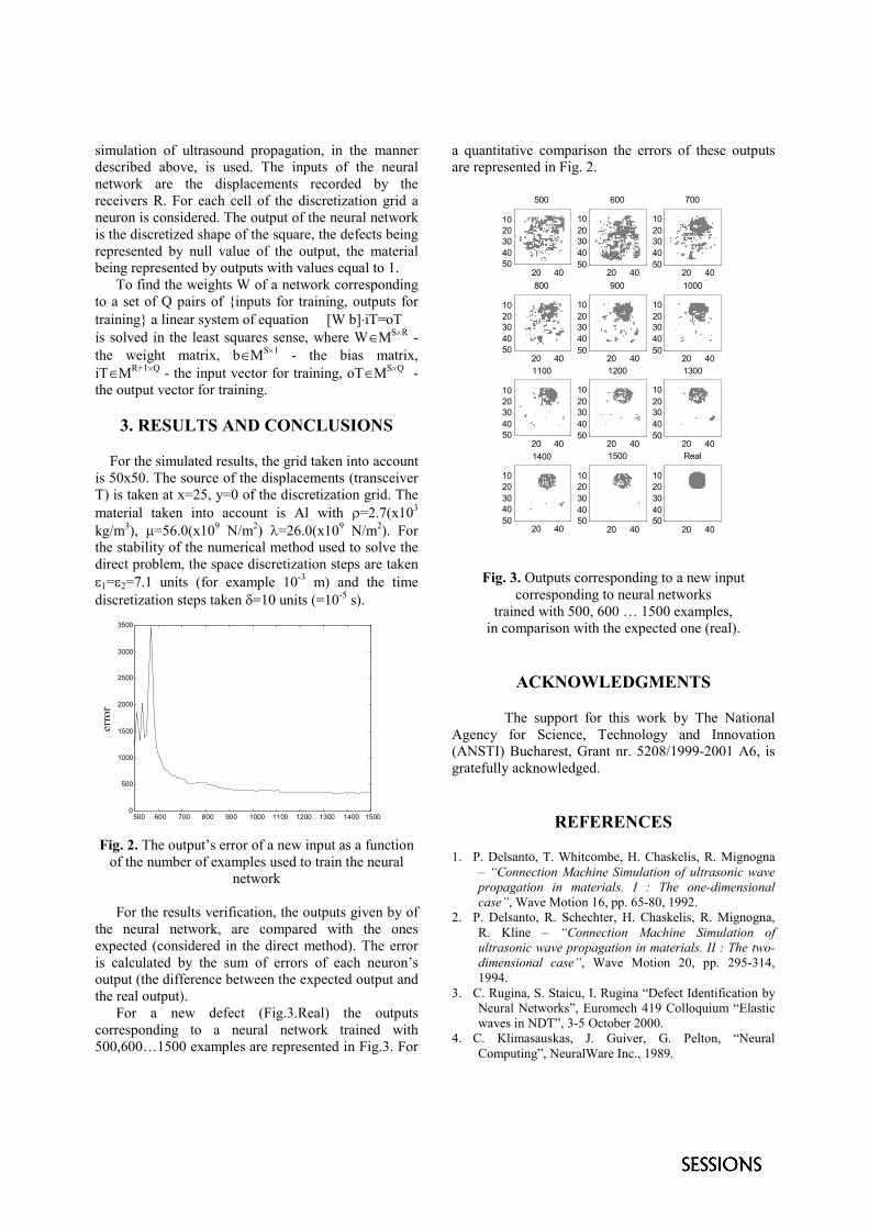
simulation of ultrasound propagation, in the mannerdescribed above, is used. The inputs of the neuralnetwork are the displacements recorded by thereceivers R. For each cell of the discretization grid aneuron is considered. The output of the neural networkis the discretized shape of the square, the defects beingrepresented by null value of the output, the materialbeing represented by outputs with values equal to 1.

To find the weights W of a network correspondingto a set of Q pairs of {inputs for training, outputs fortraining} a linear system of equation [W b]�iT=oTis solved in the least squares sense, where W�MS�R -the weight matrix, b�MS�1 - the bias matrix,iT�MR+1�Q - the input vector for training, oT�MS�Q -the output vector for training.

3. RESULTS AND CONCLUSIONS

For the simulated results, the grid taken into accountis 50x50. The source of the displacements (transceiverT) is taken at x=25, y=0 of the discretization grid. Thematerial taken into account is Al with �=2.7(x103

kg/m3), �=56.0(x109 N/m2) �=26.0(x109 N/m2). Forthe stability of the numerical method used to solve thedirect problem, the space discretization steps are taken�1=�2=7.1 units (for example 10-3 m) and the timediscretization steps taken �=10 units (=10-5 s).

500 600 700 800 900 1000 1100 1200 1300 1400 15000

500

1000

1500

2000

2500

3000

3500

erro

r

Fig. 2. The output’s error of a new input as a functionof the number of examples used to train the neural

network

For the results verification, the outputs given by ofthe neural network, are compared with the onesexpected (considered in the direct method). The erroris calculated by the sum of errors of each neuron’soutput (the difference between the expected output andthe real output).

For a new defect (Fig.3.Real) the outputscorresponding to a neural network trained with500,600…1500 examples are represented in Fig.3. For

a quantitative comparison the errors of these outputsare represented in Fig. 2.

500

20 40

1020304050

600

20 40

1020304050

700

20 40

1020304050

800

20 40

1020304050

900

20 40

1020304050

1000

20 40

1020304050

1100

20 40

1020304050

1200

20 40

1020304050

1300

20 40

1020304050

1400

20 40

1020304050

1500

20 40

1020304050

Real

20 40

1020304050

Fig. 3. Outputs corresponding to a new inputcorresponding to neural networks

trained with 500, 600 … 1500 examples,in comparison with the expected one (real).

ACKNOWLEDGMENTS

The support for this work by The NationalAgency for Science, Technology and Innovation(ANSTI) Bucharest, Grant nr. 5208/1999-2001 A6, isgratefully acknowledged.

REFERENCES

1. P. Delsanto, T. Whitcombe, H. Chaskelis, R. Mignogna– “Connection Machine Simulation of ultrasonic wavepropagation in materials. I : The one-dimensionalcase”, Wave Motion 16, pp. 65-80, 1992.

2. P. Delsanto, R. Schechter, H. Chaskelis, R. Mignogna,R. Kline – “Connection Machine Simulation ofultrasonic wave propagation in materials. II : The two-dimensional case”, Wave Motion 20, pp. 295-314,1994.

3. C. Rugina, S. Staicu, I. Rugina “Defect Identification byNeural Networks”, Euromech 419 Colloquium “Elasticwaves in NDT”, 3-5 October 2000.

4. C. Klimasauskas, J. Guiver, G. Pelton, “NeuralComputing”, NeuralWare Inc., 1989.

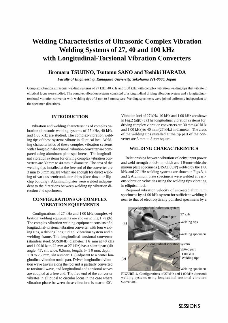
Welding Characteristics of Ultrasonic Complex VibrationWelding Systems of 27, 40 and 100 kHz

with Longitudinal-Torsional Vibration Converters

Jiromaru TSUJINO, Tsutomu SANO and Yoshiki HARADAFaculty of Engineering, Kanagawa University, Yokohama 221-8686, Japan

Complex vibration ultrasonic welding systems of 27 kHz, 40 kHz and 100 kHz with complex vibration welding tips that vibrate in

elliptical locus were studied. The complex vibration systems consisted of a longitudinal driving vibration system and a longitudinal-

torsional vibration converter with welding tips of 3 mm to 8 mm square. Welding specimens were joined uniformly independent to

the specimen directions.

INTRODUCTION

Vibration and welding characteristics of complex vi-bration ultrasonic welding systems of 27 kHz, 40 kHzand 100 kHz are studied. The complex-vibration weld-ing tips of these systems vibrate in elliptical loci. Weld-ing characteristics of these complex vibration systemswith a longitudinal-torsional vibration converter are com-pared using aluminum plate specimens. The longitudi-nal vibration systems for driving complex vibration con-verters are 30 mm to 40 mm in diameter. The area of thewelding tips installed at the free end of the converter are3 mm to 8 mm square which are enough for direct weld-ing of various semiconductor chips (face-down or flip-chip bonding). Aluminum plates were welded indepen-dent to the directions between welding tip vibration di-rection and specimens.

CONFIGURATIONS OF COMPLEXVIBRATION EQUIPMENTS

Configurations of 27 kHz and 100 kHz complex-vi-bration welding equipments are shown in Fig.1 (a)(b).The complex vibration welding equipment consists of alongitudinal-torsional vibration converter with four weld-ing tips, a driving longitudinal vibration system and awelding frame. The longitudinal-torsional converter(stainless steel: SUS304B, diameter: 16 mm at 40 kHzand 100 kHz to 22 mm at 27 kHz) has a slitted part (slitangle: 45˚, slit wide: 0.5 mm, length: 5 - 10 mm, depth:1.8 to 2.2 mm, slit number: 12) adjacent to a center lon-gitudinal vibration nodal part. Driven longitudinal vibra-tion wave travels along the rod and is partially convertedto torsional wave, and longitudinal and torsional wavesare coupled at a free end. The free end of the convertervibrates in elliptical to circular locus in the case wherevibration phase between these vibrations is near to 90˚.

Vibration loci of 27 kHz, 40 kHz and 100 kHz are shownin Fig.2 (a)(b)(c). The longitudinal vibration systems fordriving complex vibration converters are 30 mm (40 kHzand 100 kHz) to 40 mm (27 kHz) in diameter. The areasof the welding tips installed at the tip part of the con-verter are 3 mm to 8 mm square.

WELDING CHARACTERISTICS

Relationships between vibration velocity, input powerand weld strength of 0.3-mm-thick and 10-mm-wide alu-minum plate specimens (JISA1050P) welded by the 100kHz and 27 kHz welding systems are shown in Figs.3, 4and 5. Aluminum plate specimens were welded at vari-ous vibration velocities using the welding tips vibratingin elliptical loci.

Required vibration velocity of untreated aluminumspecimens by a100 kHz system for sufficient welding isnear to that of electrolytically polished specimens by a

FIGURE 1. Configurations of 27 kHz and 100 kHz ultrasonicwelding systems using longitudinal-torsional vibrationconverters.

(a)

(b)

Welding specimen

Slitted part27 kHz

Welding tips

Longitudinal vibration system

Welding specimen

Slitted part100 kHzWelding tips

Longitudinal vibration system

0

5

10

15

20

25

30

Wel

d st

reng

th ( k

gf )

0 2.5 5 7.5 10

Vibration amplitude ( µm )

0.3 mm-thick and 10 mm-widealuminum plates (JISA1100-0

Broken atspecimens part

Welding time : 5.0 s

Static clampingpressure :19 MPa

0

30

60

90

120

Inpu

t pow

er ( W

)

0

10

20

30

40

Wel

d st

reng

th ( k

gf )

0 1 2 3 4Vibration amplitude ( µm )

Static clamping force: 8.6 kgf Welding time: 3.0 s

Weld strength

0.3 mm-thick and 10 mm-widealuminum plates (JISA1100-0P

Input power

0

50

100

150

200

250

300

Inpu

t pow

er ( W

)

0

10

20

30

Wel

d st

reng

th ( k

gf )

0 0.5 1 1.5 2 2.5 3Vibration amplitude ( µm )

Welding time: 5.0 s

Static clamping force: 12.8 MPa

0.3 mm-thick and 5 mm-widealuminum plates (JISA1100-0

( Electrolytically polished )

Input powerWeld strength

Frequency:98.75 kHz

FIGURE 3. Relationship between 27 kHz vibration amplitude,and weld strength of 0.3-mm-thick and 5-mm-wide aluminumplate specimens (JISA1100P-0) (electrolytically polished).

FIGURE 4. Relationship between 40 kHz vibration amplitude,input power and weld strength of 0.3-mm-thick and 5-mm-widealuminum plate specimens (JISA1100P-0).

FIGURE 5. Relationship between 100 kHz vibrationamplitude, input power and weld strength of 0.3-mm-thick and5-mm-wide aluminum plate specimens (JISA1100P-0).

FIGURE 6. Relationship between welding time, input powerand weld strength of 0.3-mm-thick and 5-mm-wide aluminumplates (JISA1100P-0: electrolytically polished) joined by a 100kHz system.

Driving frequency : 27.478 kHz

0.2 m/s

Long

itudi

nal v

ib.v

eloc

ity0.

2 m

/s

Torsional vib.velocity0.1 m/s

0.1

m/s

0.2 m/s0.2

m/s

Torsional vib.velocity

Long

itudi

nal v

ib.v

eloc

ity

Driving frequency: 97.06 kHz

FIGURE 2. Vibration loci of 27 kHz, 40 kHz and 100 kHzcomplex vibration welding tip

27 kHz system. The required vibration velocity for weldstrength of 20 kgf is 1.2 m/s (peak-to-zero value). Therequired vibration amplitude is about 2 µm by a 100 kHzand 40 kHz and 7 µm by a 27 kHz system.

Relationship between welding time and weld strengthof 0.3-mm-thick aluminum specimens (JISA1050P, elec-trolytically polished) joined by a 100 kHz system is shownin Fig.6. The input power is rather large compared withthe other lower frequency systems due to radial vibra-tions of the driving longitudinal vibration source. Thespecimens are welded in short welding time. As weld-ing time increases, weld strength increases up to about1.0 s, but weld strength decreases by excessive long weld-ing time due to vibration fatigue.

CONCLUSION

Complex vibration ultrasonic welding systems of 27kHz, 40 kHz and 100 kHz were studied. The areas of thewelding tips installed at the tip part of the converter are 3mm to 8 mm square which are enough for direct weldingof various semiconductor chips.

Aluminum plates were welded independent to the di-rections between welding tip vibration direction andspecimens. The vibration amplitudes of the welding sys-tems required for obtaining sufficient weld strength aresmaller than a conventional linear vibration system, andbecome smaller as the vibration frequencies becomehigher. The required vibration amplitude of aluminum

plate specimens of the 100 kHz system was small-est among them. Complex vibration systems withlarger welding tip area are also under testing.

These welding systems are effective for di-rect welding of semiconductor tips of IC, LSI(face-down, flip-tip bonding) and packaging ofvarious electronic devices.

AKNOWLEDEMENTS

This work was supported by a Grant-in-Aidfor Scientific Research from the Ministry of Edu-cation, Science, Sports and Culture of Japan.

0

50

100

150

200

250

Inpu

tpow

er ( W

)

0

5

10

15

20

25

Wel

d st

reng

th ( k

gf )

0 2 4 6 8Welding time ( s )

Vibration amplitude: 1.8 µmStatic clamping force: 12.8 MPa

0.3 mm-thick and 5 mm-widealuminum plates (JISA1100-0

( Electrolytically polished )Input power

Weld strength

Frequency:98.75 kHz

(a) 27 kHz (b) 40 kHz (c) 100 kHz

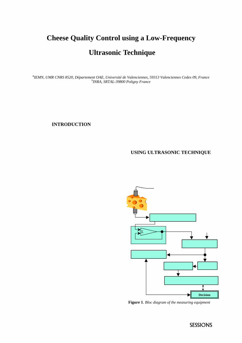
Cheese Quality Control using a Low-Frequency

Ultrasonic Technique

G. Nassara, B. Nongaillarda , L. Camusa and Y Noelb

aIEMN, UMR CNRS 8520, Département OAE, Université de Valenciennes, 59313 Valenciennes Cedex 09, FrancebINRA, SRTAL-39800 Poligny France

An ultrasonic technique using two low-frequency (30 KHz) sensors was carried out for the follow-up and thequality control of cheese in line of production. This technique, working in transmission, capable of quantifyingthe physical properties and those of the openings of cheese by taking account of the measured ultrasonicmagnitudes (velocity and attenuation) and the morphology of wave received. Some modules of signal processinganalysis applied on the measured ultrasonic magnitudes offered a precise vision on the matrix state of cheese andthe physicochemical properties of its texture.

INTRODUCTION

Many food manufacturers produce a visco-elasto-plastics media. This kind of product hasgenerally a very complex mechanical andrheological behaviour. Their physicalcharacterizations, the quality control of totalvolume product require the development of a newinstrumentation. Then, the needs in sensors in thisfield are very significant.

A quality control of the final product can beassumed through the control of manufacturingprocess steps. A product like a matured cheese forexample is generally judged some time after itsmanufacture. Its quality is in particularcharacterized by the visco-elasto-plastic propertiesof the texture as well as by the number and the sizeof the openings (in the case of some cheeses likeComté cheeses) in the structure. Then the state ofthe matrix and the quality of the cheese matterinduce causes of downgrading, which induces asignificant depreciation of the product.

Quality evaluation is carried out through severaltechniques such as percussion, coring and sampling.These methods are long, vague, delayed andintrusive. For this reason, cheese industry seek newmethods in order to evaluate the quality of theproduct as soon as possible during the process. Thenecessary corrections could thus be made, for thefuture production, in the stage of manufacture or byoptimizing the choice of conditioning like time-temperature cycles for example.

In the food industry low-intensity ultrasonicscan be used in process control applications or tomeasure acoustical properties related to the foodquality [1,2,3,4]. Ultrasonic measurements havebeen used to provide information aboutconcentration, location, structure, and physical stateof components in food materials [5].

The advantages of ultrasonic sensors andtechniques over the traditional analytical methodsare speed, nondestructivity, accuracy and fullautomation.

USING ULTRASONIC TECHNIQUE

The suggested method consists in using twoidentical ultrasonic sensors working at a 30 KHzfrequency in transmission mode. These sensors arein direct contact with the surface of cheese and thiswithout any coupling material (Figure 1).

Figure 1. Bloc diagram of the measuring equipment

Acquisition & Numeration

Normalisation

Ref

LP Filter

Average

Transmitter

Spectrum analysis

Temp. Window

Morphological analysis

Decision

Σ

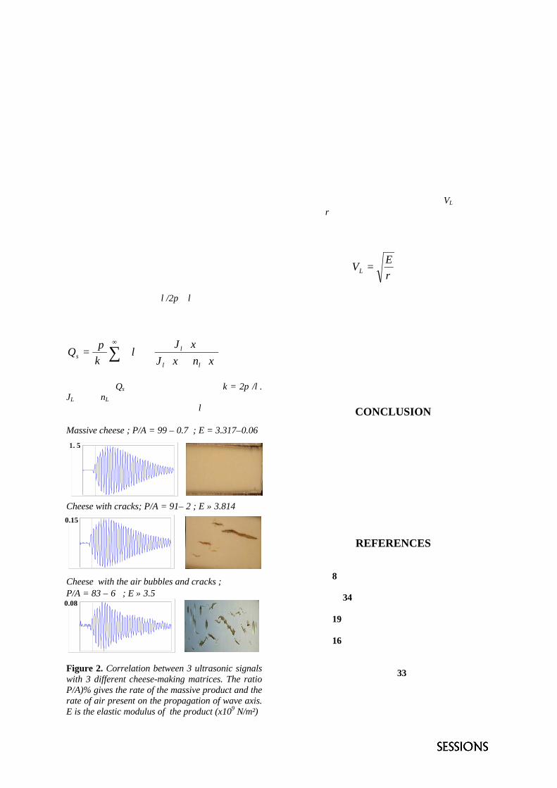
The transmitter is excited by an electric RFsignal and generate an acoustic wave, usingpiezoelectricity, which propagates in the productunder study. On the receiver, the acoustic waveinteraction with the material provides productcharacterization. This wave will be analyzed by asuitable calculation module.

The system expert placed at the output of thechain of analysis has for a purpose to make asuitable decision related to the state or the qualityof cheese.

The electronics which decides the state of thecheese matrix is based on one side on theexpression employing the rate of spectral energy tothe reception according to the rate of the openingsin the structure (1) and on the other side on themeasured ultrasonic magnitudes: velocity andattenuation.

In a viscoelastic medium, the relation bindingthe presence of the air bubbles (openings) ofdiameter R bigger than λ/2π (λ wavelength) withthe ultrasonic scattering, is given, according toNishi [ 6 ], by:

∑∞

++=

022

2

)()(

)()12(

²

4

xnxJxJ

lk

Qll

ls

π(1)

Where , Qs the ultrasonic scattering, k = 2π /λ.JL and nL are the spherical Bessel an Neumannfunctions, of the first kind of order l.

Massive cheese ; P/A = 99 ± 0.7 ; E = 3.317±0.06

Cheese with cracks; P/A = 91± 2 ; E ≈ 3.814

Cheese with the air bubbles and cracks ;P/A = 83 ± 6 ; E ≈ 3.5

Figure 2. Correlation between 3 ultrasonic signalswith 3 different cheese-making matrices. The ratioP/A)% gives the rate of the massive product and therate of air present on the propagation of wave axis.E is the elastic modulus of the product (x109 N/m²)

Figure 2 shows signals displayed by theprogram front panel employed in our step ofcharacterization.

The management of this program was workedout with the LABview software. It should be notedthat the error recorded on the state of the totalmatrix has never exceeded 2%. In other words, with1000 Comté cheeses (Jura-France), analyzed underthe same conditions, ten only were badly correlatedwith the decision given by the integrated expertsystem. This is probably related to very bad surfacequality of that cheese.

In addition, longitudinal velocity VL(m/s) anddensity ρ (Kg/m3) of cheese have made it possibleto estimate with a good approximation, the elasticmodulus E and this through the following relation:

ρE

VL = (2)

It should be noted that measurements on theelastic module gave satisfaction for a value of P/Alocated between 100% and 80%. Beyond 80% thecalculation of E was largely disturbed by themultiple diffusion of ultrasonic energy caused bythe rate of existing air on the axis of wavepropagation.

CONCLUSION

This measuring device led to an early detectionon site of texture anomaly with nondestructiveconditions (no depreciation of the product related toa sampling). Moreover, it allows on line qualitycontrol which would authorize an optimizedmanagement of storage and a relevant sorting ofcheeses at the end of refining (cut or prepackagedfor example).

REFERENCES

1. M.J.W. Povey and D.J. McClements, J. Food.Eng. 8, 217-245, (1988).

2. I. Orlindini and S. Annibaldi, Sci. Latiero-Caseria 34, 20-30, (1983).

3. S. Gunasekaran and C. Ay, J. Food Process.Eng. 19, 63-73, (1996).

4. H.O. Lee, H. Luan and D.G. Daut, J. FoodEng. 16, 127-150, (1992).

5. M.J.W. Povey, Ultrasound in Food Processing,30-65, (1998).

6. R.Y. Nishi, Acoustica 33, 65-74, (1975).

1. 5

0.15

0.08

In sonoelectrochemistry, the effects of ultrasonicirradiation on mass transport processes have beenwidely reported [1]. We recently reported that theultrasound accelerated charge transfer processes innickel deposition system [2]. The present study reportsabout effects of ultrasound on both charge transferprocess and interfacial structure in copperelectrodeposition system. The compositions of electrolyte on copperelectrodeposition were 0.5 M CuSO4 + 0.5M H2SO4and the bath temperature was controlled at (298 ± 3) K.A working electrode (WE) was of 5 mm diametercopper rod (purity 99.99%) imbedded into teflon tubingand the exposed top plane (0.20 cm2) was set apart by 2mm just under the head (1.3 cm diameter) of horn chipof ultrasonic transducer (Shimazu USP-400A, 20 kHz,400 W). A platinum wire was used as a counterelectrode and an Ag/AgCl reference electrode insaturated KCl solution was connected to cell with saltbridge separated by a chip of vycol glass. Theelectrochemical apparatus used were a potentiostat(Fuso 1100L), a function generator (Fuso HECS-321),a transient converter (Riken Denshi TCFL-8000), afrequency response analyzer (NF Electronic InstrumentS-5020), and a personal computer (NEC PC-9801VM2). WE was pretreated by polishing with#2000 emery paper and dipping for several seconds in adilute HNO3.

Results and Discussion Figure 1 shows the effects of ultrtasonic irradiationpower on polarizing curves. The stronger power led tothe more decreasing of overpotential for copperdeposition. The Eeq shifted cathodically by about ten mV

and the inflexion point on current-potential curves shifted

FIGURE 1. Effects of ultrasound on polarizing curves.Power of irradiation is 300 W/cm-2 and scan rate is 10 mV/s.

from Eeq (about 80 mV) to about –1 mA at about 45 mV withirradiation. Table 1 shows the dependence of kineticparameters obtained from Tafel plots on ultrasound.The larger power of ultrasound gave rise to the moreincreasing in the exchanging current densities�i0�andthe standard rate constant for reduction (k0), while thevalues of na (n is the number of electrons involved inrate-determining step, a is the transfer coefficient) weredecreased the more. Figure 2a shows stationarycurrents measured before and after irradiation andFigure 2b is typical current-time transient on a potentialstep chronoamperometric (PSCA) measurements. Asshown in Fig. 2a, the effects of ultrasound on cathodiccurrent changed from depression to promotion at thevicinity of Einf. As shown typically in Fig. 2b, when

The Effects of Ultrasound on Faradaic Processes and theInterfaces of Metal-Electrolyte in Copper Electrodeposition

SystemsK. Kobayashia, A. Chibaa, K. Tsuzukia and N. Minamib

aDepartment of Materials Chemistry, Yokohama National University79-5,Tokiwadai, Hodogaya-ku, Yokohama 240-8501, Japan

bDivision of Research & Development, Tokyo Cathode Laboratory Co., Ltd.25-33, Miyako, Namegawa, Hiki-Gun, Saitama, 355-0812, Japan

It was shown by various electrochemical methods that ultrasound accelerated charge transfer processes in copperelectrodeposition systems. The imposition of ultrasound led to both the negative shift of the equilibrium potential (Eeq) and thenegative shift of the potential of inflexion point�Einf�on current-potential curve by several tens of mV relative to Eeq. The effectsof ultrasound on stationary cathodic currents after potential-stepped changed from depression at more positive stepped potentialsto acceleration at more negative stepped potentials than Einf. The results of faradaic impedance (FI) measurements showed thatthe irradiation of ultrasound increased both faradaic current for reduction and capacitance of the double layer at the metal-electrolyte interface. These results suggest that the ultrasound decreased the thickness of the outer Helmholtz layer at theinterface and accelerated the rate of reduction process. The negative shift of Einf and the decrease of the transfer coefficientsmay be able to be interpreted by Frumkin effect.

-0.100.1

-15

-10

-5

0

Electrode potential / V vs. Ag/AgCl

Cath

odic

cur

rent

/ m

A

no irradiation

40% of power

70% of power

inflexion point

stepped at more positive potentials than Einf, thecathodic currents decreased with irradiation andincreased to somewhat larger values than stationaryvalues with cutoff of irradiation. On the other hand,when stepped at more negative potentials, thoseincreased with irradiation and furthermore increasedslightly even with cutoff of irradiation while thosedecreased gradually to the stationary values withirradiation. Table 2 shows the values ofelectrochemical parameters obtained from FImeasurements. The imposition of ultrasound causedboth the decrease in faradaic charge transfer resistance(Rct), that is, the increase in faradaic currents (If ) andthe increase in capacitance of double layer at the metal-electrolyte interface. These results suggest thatultrasonic irradiation caused the decrease in thicknessof outer Helmholtz layer so that the rate of reductionprocess was accelerated. The negative shift of Einf,from Eeq, the change from depression to promotion at

Table 1. Dependence of electrochemical kinetic parameterson irradiation power

Power i0 na k0 % / Acm-2 / cm s-1

0 5.9×10-4 0.82 6.1×10-6

10 4.0×10-3 0.46 4.1×10-5

40 5.1×10-3 0.40 5.2×10-5

70 6.4×10-3 0.38 6.6×10-5

Table 2. Electrochemical parameters obtained from faradaicimpedance method E U.S.* Rsol Rct Cdl If

/ V / ohm / ohm /10-6F /A cm-2

0.06 off 4.3 249 1.9 6.5×10-4

0.06 on 5.1 195 3.4 8.2 ×10-4

0.04 off 5.6 209 1.8 7.7×10-4

0.04 on 6.6 120 3.8 1.3×10-3

0.02 off 5.7 251 1.4 6.4×10-4

0.02 on 5.4 153 2.6 1.0×10-3

0.00 off 7.1 173 1.4 9.3×10-4

0.00 on 5.6 59 3.1 2.7×10-3

-0.02 off 6.3 134 1.5 1.2×10-3

-0.02 on 5.9 58 2.3 2.8×10-3

-0.04 off 5.8 72 2.2 2.2×10-3

-0.04 on 4.3 20 3.3 7.9×10-3

-0.06 off 5.0 48 2.6 3.3×10-3

-0.06 on 4.2 20 4.4 8.0×10-3

*U.S. is ultrasonic irradiation. A.c. amplitude was 10 mVand frequencies measured were from 100 Hz to 20 kHz.

FIGURE 2. Current transient with irradiation in PSCA.a) Current-potential plots b) Current-time transient. Eachpotential was stepped from 95 mV and the sampling time was0.3 ms.

Einf, and the decrease of na with irradiation may beable to be interpreted by the Frumkin effects.

REFERENCES

1. J.C. Ball and R.G. Compton, Electrochemistry 67�912-919 (1999).2. K. Kobayashi, A. Chiba, and N. Minami, Ultrasonics 38, 676-681

(2000).

0 5 10 15

-1

-0.5

0

on

at 70 mV

at 10 mV

off on off

on off on off

mA

s

-100-50050

-5

-4

-3

-2

-1

0

Electrode potential / mV vs. Ag/AgCl

Cath

odic

cur

rent

/ m

A

a)

b) irradiation

no irradiation

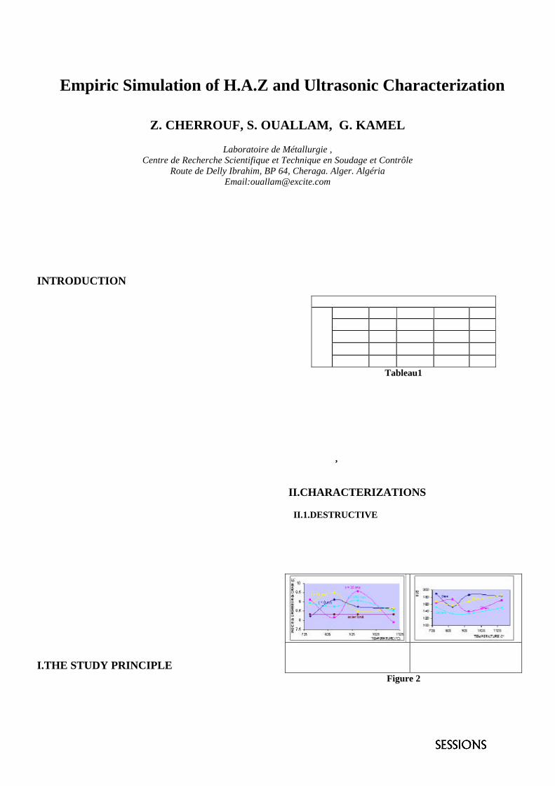
1

Empiric Simulation of H.A.Z and Ultrasonic Characterization

Z. CHERROUF, S. OUALLAM, G. KAMEL

Laboratoire de Métallurgie ,

Centre de Recherche Scientifique et Technique en Soudage et Contrôle Route de Delly Ibrahim, BP 64, Cheraga. Alger. Algéria

Email:ouallam@excite.com During the welding operations, heat supply generates metallurgical phenomena which are difficult to control because of the great thermal gradient , that generates structural transformations and phases transformations some of which are harmful to the welded sets. This is why we have simulated these effects by specific thermal treatments on the E24. These treatments have allowed us to get an information set serving as data base for a welding sequence metallurgical phenomena analysis and also by a destructive and no destructive investigation methods characterisation proceeding.

INTRODUCTION

In welding the material behaviour at a heat time contribution generates some complex and unverifiable structural variations on a variable distance according to the process type used . This zone called heat affected zone (HAZ) is the physico - chemical variation support, of, mechanical feature variations and lead to simulate proceed necessity by thermal treatments to the main temperatures characteristic of this zone [1] This method is very useful for us to understand the metallurgic mechanisms in the HAZ as magnification, the precipitate, the fragility, etc.… Because these phenomena and her consequences cannot be analysed easily on real soldering for high micro structural gradient. For a same steel, being differently thermally treated, to find at an interrelationship between the different characterizations, as well the destructive techniques set that the non destructive procedures one, would drive to establish a simple and efficient basis in the welding structural transformations in metallurgy phenomena understanding. The first part work [1], gives results about destructive tests characterization. In the second part, the objective is to see the metallurgical transformations influence mislead on an elastic wave having crossed the considered zone. The non destructive investigating techniques as ultrasonic are much more used in materials characterization for mechanical property parameters determination. however this domain remains still actual, and this for the parameters diversity going in game. In fact, several studies were interested in the residual constraint assessment by joining the effort applied in one materials to the ultrasonic velocity variation in the effort direction [2], others, on the grain size effect on the ultrasonic waves attenuation [3]. I.THE STUDY PRINCIPLE : It takes a usual thermal treatments set as a basis (tab 1) applied to a E24 type, high thickness construction steel with high elastic limit according to the NFA35.501, used in the

gas spheres storage construction that requires some heat treatments after welding.

Maintenance time 0mn 30mn 1h30 4h 750°C A B C D 850°C A1 B1 C1 D1 950°C A2 B2 C2 D2

T°C

of

H.T

1100°C A3 B3 C3 D3 Tableau1

This objective simulation has to produce some microstructures susceptible to occur in a multi - passes soldering or by post welding heat treatments. After sixteen samples specific heat treatments , some destructive and non destructive investigations have been undertaken while insisting on the parameter influence appreciation, maintaining times and temperatures, in relation to the reference sample intrinsic features. II.CHARACTERIZATIONS II.1.DESTRUCTIVE it allow to understand phases transformations (by metallografic observation and the grain indices assessment ), the mechanical properties of hardness and ductility (by hardness and the resilience measure ) fig 2

Grain indices(G) evolution according to the T°C of heat treatment

HV5 according to the T°C of heat treatment

Figure 2 The study showed in particular, that curves presented a singular point to 900°C witch represent the best features of grain seize, and resilience. [1]

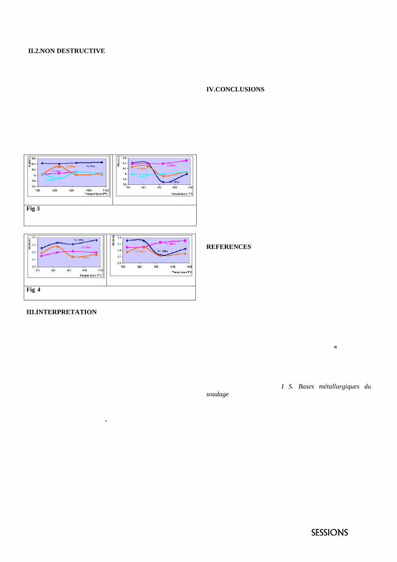
2

II.2.NON DESTRUCTIVE In our work ,we were interested in the metallurgic phenomena effect generated by the heat treatments on ultrasonic velocity .two methods were used ,by transmission and by in immersion Echo at four (04) different frequencies. The essential result is to recover the same singular point than the destructive tests. It is verified by the Hall and Petch relation[4] witch express the dependence between the grains size , in particular, and the yield strength. so the intersection point corresponds to the best heat treatment of the media witch is homogeneous, isotropic and non dispersal in us point of view ..Fig3 and Fig4

Maintenance time 0min

Maintenance time 240mn

Fig 3 the longitudinal waves velocity Vl evolution according to the

heat treatment Temperature for 1Mhz, 2Mhz, 5Mhz and 10Mhz

Maintenance time 0min

Maintenance time 240mn

Fig 4 Transversal waves velocity Vt evolution according to the heat treatment temperature for 1Mhz, 2Mhz, 5Mhz frequencies III.INTERPRETATION The curves analysis (Fig2 ,Fig3, Fig4) show a certain interrelationship between the ultrasonic waves behaviour with the metallurgic and mechanical properties obtained during these heat treatments. It is the 750°C temperature case observed and 0mn maintained time where the transformation phase is partial and do not show any increase of the grain size and the velocity waves is practically negligible .It is not the 850°c temperature case where the velocity increases for 2MHz and decrease for10MHz whereas it remains stationary for 1MHz and 2MHz frequencies. For the 240min maintained time we have noted a Vl velocity reduction, specially at 1Mhz frequency and beyond 850°C temperature. This can be explained by material fragility reduction observed on metallographic which show a decarburising so a reduction of Vickers hardness HV5 and of course increase of resilience. The question is, to confirm this evolution in relation to these phases transformations generated.

This report is as valid for the case for transverse waves velocities (Vt). It is necessary to signal that ultrasonic signal was not obtained for 10MHz frequency for the transverse waves velocities IV.CONCLUSIONS Among all existing curve tracing possibilities ,the choice was made on those who the ultrasonic parameters according to the temperature for a constant maintained time and frequencies. So all formulated interpretation is subjected to be completed in one way or another. Knowing that the relative error of ultrasonic velocity is 100m/s, observations are the following: - The ultrasonic wave propagates itself in a middle inhomogeneous that cannot be considered like isotropy; - The size of grain, the rate of constraints interns, rates of phases in presence (ferrite, perlite), structural morphology type of should be taken into consideration; - The middle is dispersed, the wave velocity present variations according to the frequency; Cases of longitudinal and transverse speed values to points (950°C,30mn,5MHz) and (950°C,240mn,1MHz) should be studied deeper.

REFERENCES [1] Z.cherrouf ,S.Ouallam, G.kamel ,N .ouali « Simulation Empirique de la ZAT d’une Soudure par Traitement Thermique Spécifique sur du E24 » . Journée de mécanique. Ecole Militaire Polytechnique 2000 .Alger 25-26/11/2000 [2] Y.Abdellahoui, H.walaszek ,C.Peyrac ,H.P.lieurade ,M.Cherfaoui « Apport des Ultrasons dans l’Optimisation des Procédure de Soudage » Rev. soudage et techniques connexes .Septembre –octobre1999 [3] Z.cherrouf, N.Ouali , S.ouallam , G.Kamel« The steel grain Magnification Thermal Processing on the Defects Detection in Steel by Ultrasonic » .15Th world conference on non destructive testing- Roma 15-21October2000-10-24 [4] H.GRANJON., « I S. Bases métallurgiques du soudage » publications de la soudure autogène . pages 17-57

Ultrasonic Composite Transducer for NondestructiveTesting of Concrete

C. Micleaa, C. Tanasoiua, A. Gheorghiub, C.F. Micleaa, V. Tanasoiua

aNational Institute for Materials Physics, 96700 Magurele-Bucharest, POBox MG-7, ROMANIAbHyperion University, Faculty of Physics, Bucharest, ROMANIA

The construction and the main characteristics of a PZT ceramic-steel composite transducer destined for nondestructive testingand evaluations of concrete and rocks are presented. A detailed description of the way in which this goal was attained is included.Basic electrical and acoustical measurements have been perfomed and an iterative method for the determination of the workingfrequency has been inferred. The results are displayed in both acoustical and electrical spectra with the resolved equivalent circuitincluded. Experiments using such transducers are proposed.

1. INTRODUCTION

Ultrasonics is able to furnish nondestructive testingtechniques for different materials [1]. It is also used todetect cracks in forged parts and railway lines, or tomeasure the wall thicknesses of laminated sheets. Eachkind of measurement or testing needs a specifictransducer adapted to the kind of material and to itsshape and physical characteristics [2]. The present work reports on the construction andcharacteristics of an ultrasound transducer, with theworking frequency around 40 kHz, used to inspect theconcrete structures either cast on site or in massproduction of prefabricated units.

2. CONSTRUCTION AND WORKINGPRINCIPLES

The technical solution chosen for our transducerwas dictated by the necessity to have the workingfrequency around 40 kHz, since the intrinsicinhomogeneities of the concrete structures limit theupper frequency to somewhere around 50 kHz [3].Consequently, we chose a composite type transducermade of piezoceramic elements and a steel cylinderglued together as shown schematically in figure 1.

FIGURE 1. Schematic view of the transducer

The main parts of the transducer are as follows: sixpiezoceramic discs (1), of 22 mm diameter and 3 mm

thickness are glued in a “sandwich” structure. Theyrepresent the “hot part” of the mechanical oscillator; asteel cylinder (2) with 22 mm diameter and 17 mmthickness, backs the piezoelectric “sandwich” andrepresents the “cold part” of the transducer; a frontmechanically protecting thin (1 mm) steel disc (3), forprotection at the interaction with the rough surface tobe investigated; electrical connections (4) and theprotection case (5). For a single disc, the fundamental thickness mode isin the range of 600 kHz. At this frequency of theacoustic spectrum low order overtones of the radialmode are also present and they will interfere with thefundamental one in a mode coupling process. The usualworking frequency for concrete structures must beunder 100 kHz and in order to reach such values weused the simple solution of six individual discs glued ina “sandwich” structure. In this way the electricalconnections are disposed in derivation and each discreceives a six times smaller e.m.f., which lead to aconsiderable simplification of the electronics.Furthermore, the frequency is still lowered through thelengthening of the system by a passive “cold” material.The steel cylinder is tightly glued to the piezoelectric“sandwich”, which results in a final lengthening ofabout 35 mm, which corresponds to a fundamentalfrequency, for the longitudinal mode, of about 40 kHz. The transducer produces ultraacustic wave packets,which are emitted through the frontal part, into thespecimen. The echo produced by any defect of theinvestigated material, is received with a time delay τ,attenuated and distorted. This change in the pattern ofthe wave packet represents the encrypted history of thematerial’s behavior to the ultrasounds.

3. MEASUREMENTSThe electrical measurements of the transducer were

performed by means of an impedance analyzer, typeHP-4194A. The electrical spectra are displayed infigure 2. From the practical point of view it is veryimportant to know the value of the actual working

4

4

25513

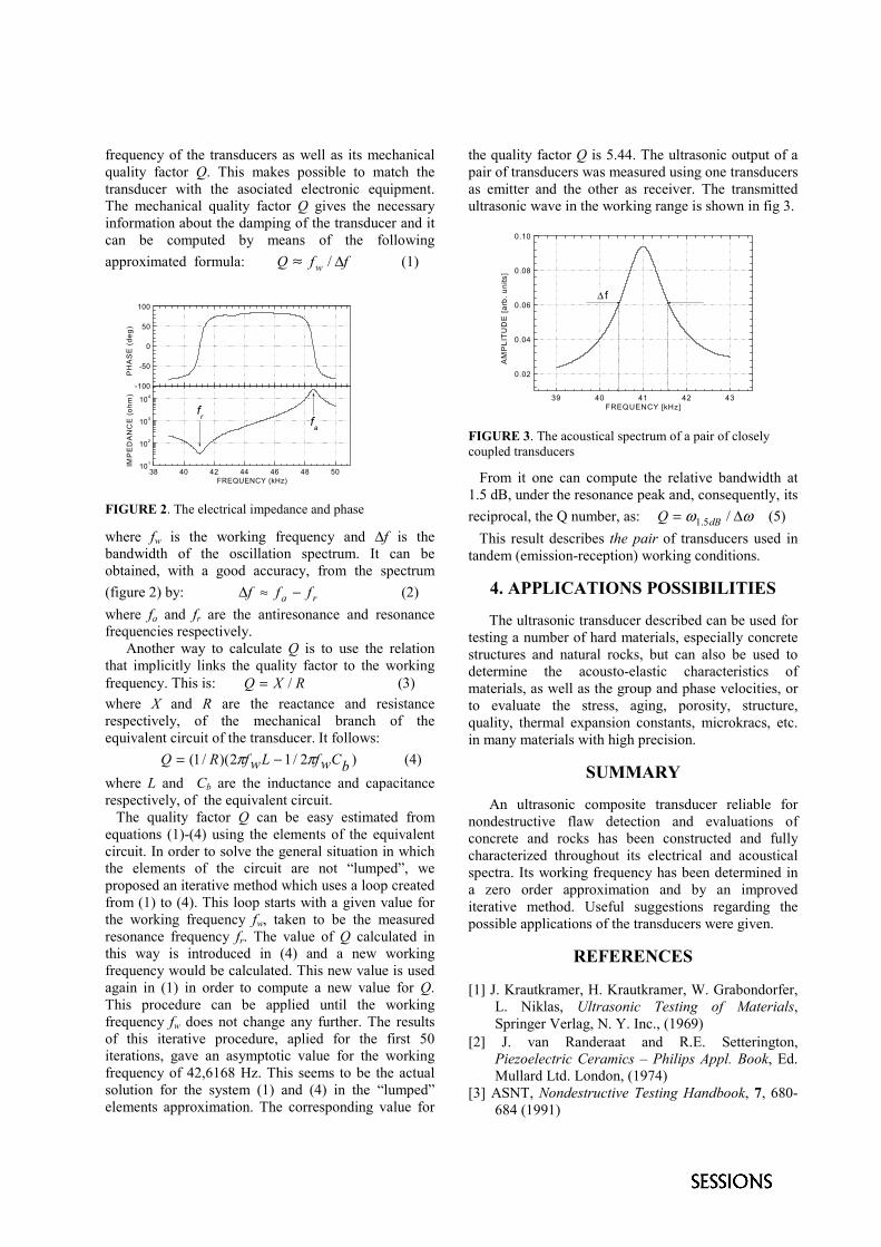
frequency of the transducers as well as its mechanicalquality factor Q. This makes possible to match thetransducer with the asociated electronic equipment.The mechanical quality factor Q gives the necessaryinformation about the damping of the transducer and itcan be computed by means of the followingapproximated formula: ffQ w ∆≈ / (1)

FIGURE 2. The electrical impedance and phase

where fw is the working frequency and ∆f is thebandwidth of the oscillation spectrum. It can beobtained, with a good accuracy, from the spectrum(figure 2) by: ra fff −≈∆ (2)where fa and fr are the antiresonance and resonancefrequencies respectively.

Another way to calculate Q is to use the relationthat implicitly links the quality factor to the workingfrequency. This is: RXQ /= (3)where X and R are the reactance and resistancerespectively, of the mechanical branch of theequivalent circuit of the transducer. It follows:

)2/12)(/1( bCwfLwfRQ ππ −= (4)where L and Cb are the inductance and capacitancerespectively, of the equivalent circuit. The quality factor Q can be easy estimated fromequations (1)-(4) using the elements of the equivalentcircuit. In order to solve the general situation in whichthe elements of the circuit are not “lumped”, weproposed an iterative method which uses a loop createdfrom (1) to (4). This loop starts with a given value forthe working frequency fw, taken to be the measuredresonance frequency fr. The value of Q calculated inthis way is introduced in (4) and a new workingfrequency would be calculated. This new value is usedagain in (1) in order to compute a new value for Q.This procedure can be applied until the workingfrequency fw does not change any further. The resultsof this iterative procedure, aplied for the first 50iterations, gave an asymptotic value for the workingfrequency of 42,6168 Hz. This seems to be the actualsolution for the system (1) and (4) in the “lumped”elements approximation. The corresponding value for

the quality factor Q is 5.44. The ultrasonic output of apair of transducers was measured using one transducersas emitter and the other as receiver. The transmittedultrasonic wave in the working range is shown in fig 3.

FIGURE 3. The acoustical spectrum of a pair of closelycoupled transducers

From it one can compute the relative bandwidth at1.5 dB, under the resonance peak and, consequently, itsreciprocal, the Q number, as: ωω ∆= /5.1 dBQ (5) This result describes the pair of transducers used intandem (emission-reception) working conditions.

4. APPLICATIONS POSSIBILITIES

The ultrasonic transducer described can be used fortesting a number of hard materials, especially concretestructures and natural rocks, but can also be used todetermine the acousto-elastic characteristics ofmaterials, as well as the group and phase velocities, orto evaluate the stress, aging, porosity, structure,quality, thermal expansion constants, microkracs, etc.in many materials with high precision.

SUMMARY

An ultrasonic composite transducer reliable fornondestructive flaw detection and evaluations ofconcrete and rocks has been constructed and fullycharacterized throughout its electrical and acousticalspectra. Its working frequency has been determined ina zero order approximation and by an improvediterative method. Useful suggestions regarding thepossible applications of the transducers were given.

REFERENCES

[1] J. Krautkramer, H. Krautkramer, W. Grabondorfer,L. Niklas, Ultrasonic Testing of Materials,Springer Verlag, N. Y. Inc., (1969)

[2] J. van Randeraat and R.E. Setterington,Piezoelectric Ceramics – Philips Appl. Book, Ed.Mullard Ltd. London, (1974)

[3] ASNT, Nondestructive Testing Handbook, 7, 680-684 (1991)

39 40 41 42 43

0.02

0.04

0.06

0.08

0.10

∆ f

AM

PLI

TU

DE

[arb

. uni

ts]

FREQUENCY [kHz]

38 40 42 44 46 48 50101

102

103

104

fafr

IMP

ED

AN

CE

(ohm

)

FREQUENCY (kHz)

-100

-50

0

50

100

PH

AS

E (

deg)

FAULT DETECTION IN AUTOVEHICLE USING ACOUSTIC SIGNAL PROCESSING

G. Cammarata, G. Fargione, A. Fichera, A. Pagano. A. Risitano

Dip. di Ingegneria Industriale e Meccanica – Università di Catania, Viale A. Doria 6, 95125 Catania, Italy Tel. +39 095 7382450; Fax +39 095 337994, afichera@ift.ing.unict.it apagano@ift.ing.unict.it

This paper aims to present the preliminary results of a new methodology, based on the analysis of externally measured acoustic signals, for the early fault diagnosis in autovehicles. The methodology move from a wide set of experimental tests, performed according to specified test conditions, and collecting acoustic measurements detected on autovehicles presenting no fault as well as autovehicle affected by specific faults. The experimental sound pressure level (SPL) was analysed through two steps: the extraction of the wavelet coefficients, which accounted for the time-frequency characterisation of each experimental time series, and the clustering of the experimental whole set of tests through Kohonen associative memories. The second step, in particular, aimed at creating clusters of tests having distinct wavelet coefficients (i.e. time-frequency behaviours). Finally, the clusters obtained were compared both with the classes collecting autovehicles affected by faults and with those collecting functioning autovehicles. Reported results show the ability of the methodology to address the problem of fault detection.

INTRODUCTION

The possibility to forecast the occurrence of process or component faults represents an important issue in many industrial and automotive applications. The aim of this study is to define an innovative methodology for the fault diagnosis in autovehicles. The proposed approach is based on the application of recently developed soft-computing techniques to the analysis of experimental measurements.

The first step of this study consisted in performing an extensive set of experimental measurements on a sufficiently wide sample of similar autovehicles. The experimental time series were therefore described by means of Wavelet Analysis and their dominant features where extracted. In this way, each experimental test was associated to a vector of features able to give a complete characterisation of its dynamics.

The last step consisted in clustering these vectors by means of a Kohonen Associative Memory. This is a neural network structure whose training is performed in a unsupervised fashion and which possess peculiar and interesting characteristics, particularly useful in the present application.

Obtained results show interesting capability for future applications of the proposed methodology as a general strategy for fault diagnosis.

EXPERIMENTAL TEST GRID

The experimental apparatus consisted of a real-time Larson & Davis phonometer, model 2900 [1], measuring the SPL. It was used to detect, at a frontal distance from the source of 0.7 m, the SPL generated by each of the 30 autovehicles forming the experimental test grid. The length of each test was set at 240 s for a sampling frequency of 20 Hz. In order to ensure standard testing condition for the

whole test grid, the vehicles were tested at the lowest regime conditions, corresponding to an angular velocity of the crankshaft ranging from 950 to 1000 rpm. The experimental test grid was made of 65 tests performed over 30 different samples of the same autovehicles (FIAT Punto) having the same cubic capacity (1242 cm3) and a mileage ranging from 1000 to 15000 km. The experimental test grid was appositely chosen to be formed by 28 “normal” vehicles, i.e. vehicles not affected by strong malfunctioning, and two “failing” vehicles, i.e. vehicles characterised by a relevant problem (in particular, the burn-out of one of the bearings).

WAVELET FEATURE EXTRACTION

The aim of this section is to describe the reasons why wavelet analysis was chosen for features extraction. For an exhaustive description of the theory behind wavelet analysis see [2].

The basic idea consists in analysing the experimental time series applying one of the possible Wavelet Transformation, in order to calculate a limited number of coefficients describing each test. Wavelet analysis allows the characterisation of the signal in the time-frequency domain, which is much more accurate of what can be obtained by means of Fourier Analysis in the time-frequency domain. In fact, the use of FFT would require the choice of a limited number of fixed frequency and the analysis of the corresponding amplitudes; this problem can be hardly addressed as the dominant frequencies characterising each experimental test are in general different from one another and may depends by external factor. On the other hand, wavelet analysis operates by associating a coefficient to separated frequency bands and, therefore, performs a synthetic characterisation of frequency bands and release from the choice of the frequencies to be analysed.

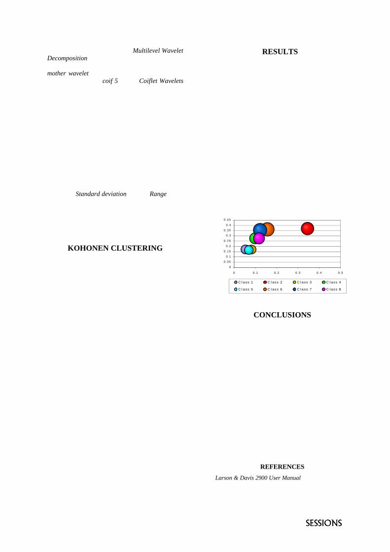
In this study, the approach of Multilevel Wavelet Decomposition was chosen [2], opportunely defining the maximum decomposition level and the mother wavelet. In particular, the mother wavelet herein used was the coif 5, of the Coiflet Wavelets family [2], which has an impulsive nature and was likely to well approximate the time series detected on autovehicle known to be affected by failures. The maximum decomposition level was set to five, which was considered a satisfactory compromise between a sufficiently small number of features and an adequate characterisation of the experimental time series.

Once the wavelet decomposition is performed, a vector of ordered coefficients can be associated to each experimental test. In particular, each vector was made of 15 components, obtained calculating three statistical parameters for each of the five levels of detail. The statistical parameters are the Mean, the Standard deviation and the Range of the time series (amplitude excursion between the maximum and the minimum of the signal).

This vector characterises the state of the process and is likely to be able to give useful information on weather there is a failure or not.

KOHONEN CLUSTERING

Kohonen associative memories (or maps) are neural networks that are trained in an unsupervised modality, i.e. without the influence of the external environment [3]. They can be used to autonomously reveal the existence of similarities in the components of the input vectors and are trained to associate to similar input vectors a specific cluster. The number of neurons of the Kohonen layer corresponds to the number of clusters in which the neural network can map the vectors of the input space. Here it is just mentioned that the existence of inter-layer connections typical of Kohonen maps is useful to give an ordered structure to the output space (i.e. to the clusters), namely self organisation. Using this neural structure, output neurons close to one another correspond to physically similar clusters; vice versa distant clusters represent classes of input vectors characterised by different behaviours. Details on Kohonen maps can be found in [3]. In this study, the vectors collecting the wavelet coefficients were used to train several Kohonen maps in order to cluster the test related to the various autovehicles contained in the experimental matrix according to the similarities shown by the features describing their behaviours.

The optimal clustering was considered that obtained with a 8 neurons Kohonen layers, trained for 10000 epochs.

RESULTS

Figure 1 reports the results of the optimal clustering. Obviously, it is necessary to find an adequate representation, as it is not possible to consider all of the 15 components that represent each experimental test. Therefore, it was chosen here to consider only those three components for which the greatest variations occurred in the whole test grid, which are those whose effect mainly enhances the separation in different clusters. Of these components, two were used as coordinated axes and the third was used as radius of a ball centred in the points of this plane. It can be noticed from the figure that there is one of the class that is indeed well separated from the other (namely class two, corresponding at the top right ball of the plot). This is an important result; in fact, class two collects the tests manifesting a specific mechanical failures, i.e. the above mentioned bearing burn-out. Here it is just mentioned that classes 1-3-5, which form a separate group in Figure 1, collect the experimental tests manifesting a malfunctioning due to spark plug

0

0.05

0.1

0.15

0.2

0.25

0.3

0.35

0.4

0.45

0 0.1 0.2 0.3 0.4 0.5

C lass 1 C lass 2 C lass 3 C lass 4

C lass 5 C lass 6 C lass 7 C lass 8

Fig.1 Separation of the clusters created by the Kohonen map.

CONCLUSIONS

This paper presents a preliminary study of an innovative methodology for fault detection, herein developed for autovehicles. The approach consists in applying to the experimentally detected acoustic time series the modern analytic tools offered by wavelet analysis and neural networks. A wide set of experimental acoustic tests were acquired by means of a phonograph on various autovehicles, a few of which were affected by specific failures.

Statistical information on the behavior of wavelet coefficients were therefore associated to each experiment, in order to be characterise its dynamics in a reliable way. This information wer finally used to cluster the whole set of experimental tests in a few classes in an unsupervised modality. The results of the clustering show that the proposed methodology is able to address with satisfactorily confidence authovehicle fault diagnosis

REFERENCES

[1] Larson & Davis 2900 User Manual, L. & D. Inc, (1992). [2] Donoho, D., Proc. of Symp. in Appl. Math., V. 47, USA, pp. 173-178 (1993). [3] Kohonen T. Self-Organizing Maps, Spr.-Ver., 1995.

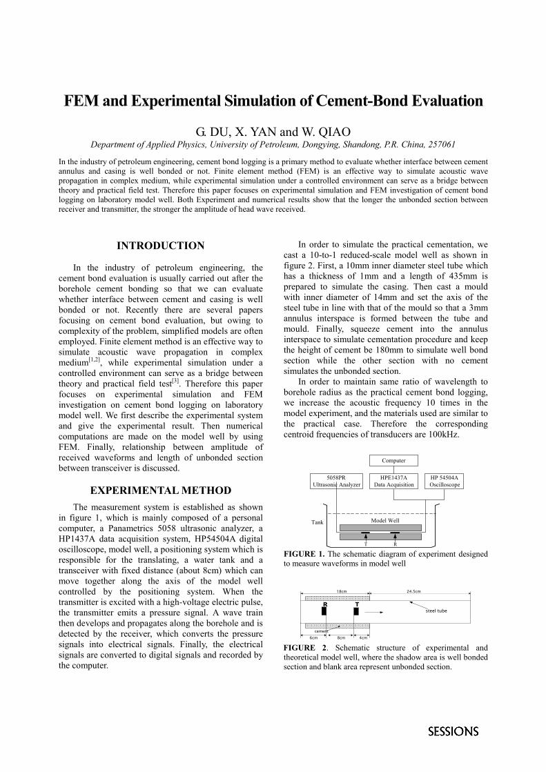
FEM and Experimental Simulation of Cement-Bond Evaluation

G. DU, X. YAN and W. QIAODepartment of Applied Physics, University of Petroleum, Dongying, Shandong, P.R. China, 257061

In the industry of petroleum engineering, cement bond logging is a primary method to evaluate whether interface between cementannulus and casing is well bonded or not. Finite element method (FEM) is an effective way to simulate acoustic wavepropagation in complex medium, while experimental simulation under a controlled environment can serve as a bridge betweentheory and practical field test. Therefore this paper focuses on experimental simulation and FEM investigation of cement bondlogging on laboratory model well. Both Experiment and numerical results show that the longer the unbonded section betweenreceiver and transmitter, the stronger the amplitude of head wave received.

INTRODUCTION

In the industry of petroleum engineering, thecement bond evaluation is usually carried out after theborehole cement bonding so that we can evaluatewhether interface between cement and casing is wellbonded or not. Recently there are several papersfocusing on cement bond evaluation, but owing tocomplexity of the problem, simplified models are oftenemployed. Finite element method is an effective way tosimulate acoustic wave propagation in complexmedium[1,2], while experimental simulation under acontrolled environment can serve as a bridge betweentheory and practical field test[3]. Therefore this paperfocuses on experimental simulation and FEMinvestigation on cement bond logging on laboratorymodel well. We first describe the experimental systemand give the experimental result. Then numericalcomputations are made on the model well by usingFEM. Finally, relationship between amplitude ofreceived waveforms and length of unbonded sectionbetween transceiver is discussed.

EXPERIMENTAL METHODThe measurement system is established as shown

in figure 1, which is mainly composed of a personalcomputer, a Panametrics 5058 ultrasonic analyzer, aHP1437A data acquisition system, HP54504A digitaloscilloscope, model well, a positioning system which isresponsible for the translating, a water tank and atransceiver with fixed distance (about 8cm) which canmove together along the axis of the model wellcontrolled by the positioning system. When thetransmitter is excited with a high-voltage electric pulse,the transmitter emits a pressure signal. A wave trainthen develops and propagates along the borehole and isdetected by the receiver, which converts the pressuresignals into electrical signals. Finally, the electricalsignals are converted to digital signals and recorded bythe computer.

In order to simulate the practical cementation, wecast a 10-to-1 reduced-scale model well as shown infigure 2. First, a 10mm inner diameter steel tube whichhas a thickness of 1mm and a length of 435mm isprepared to simulate the casing. Then cast a mouldwith inner diameter of 14mm and set the axis of thesteel tube in line with that of the mould so that a 3mmannulus interspace is formed between the tube andmould. Finally, squeeze cement into the annulusinterspace to simulate cementation procedure and keepthe height of cement be 180mm to simulate well bondsection while the other section with no cementsimulates the unbonded section.

In order to maintain same ratio of wavelength toborehole radius as the practical cement bond logging,we increase the acoustic frequency 10 times in themodel experiment, and the materials used are similar tothe practical case. Therefore the correspondingcentroid frequencies of transducers are 100kHz.

Tank

5058PRUltrasonic Analyzer

Computer

HPE1437AData Acquisition

Model Well

HP 54504AOscilloscope

T R

FIGURE 1. The schematic diagram of experiment designedto measure waveforms in model well

18cm 24.5cm

cement

TR

6cm 8cm 4cm

steel tube

FIGURE 2. Schematic structure of experimental andtheoretical model well, where the shadow area is well bondedsection and blank area represent unbonded section.

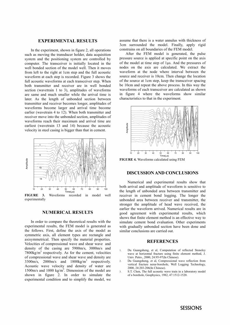
EXPERIMENTAL RESULTS

In the experiment, shown in figure 2, all operationssuch as moving the transducer holder, data acquisitionsystem and the positioning system are controlled bycomputer. The transceiver is initially located in thewell bonded section of the model well. Then it movesfrom left to the right at 1cm step and the full acousticwaveform at each step is recorded. Figure 3 shows thefull acoustic waveforms at each transceiver step. Whenboth transmitter and receiver are in well bondedsection (wavetrain 1 to 3), amplitudes of waveformsare same and much smaller while the arrival time islater. As the length of unbonded section betweentransmitter and receiver becomes longer, amplitudes ofwaveforms become larger and arrival time becomeearlier (wavetrain 4 to 12). When both transmitter andreceiver move into the unbonded section, amplitudes ofwaveforms reach their maximum and arrival time areearliest (wavetrain 13 and 14) because the acousticvelocity in steel casing is bigger than that in cement.

10 20 30 40 50 60 70 80 90 100

10

5

14

1

Ampl

itude

Time(�s)FIGURE 3. Waveforms recorded in model wellexperimentally

NUMERICAL RESULTS

In order to compare the theoretical results with theexperimental results, the FEM model is generated asthe follows. First, define the axis of the model assymmetric axis, all element types are rectangle andaxisymmetrical. Then specify the material properties.Velocities of compressional wave and shear wave anddensity of the casing are 5900m/s, 3000m/s and7800kg/m3 respectively. As for the cement, velocitiesof compressional wave and shear wave and density are3300m/s, 2000m/s and 1800kg/m3 respectively.Acoustic wave velocity and density of water are1500m/s and 1000 kg/m3. Dimension of the model areshown in figure 2. In order to simulate theexperimental condition and to simplify the model, we

assume that there is a water annulus with thickness of3cm surrounded the model. Finally, apply rigidconstrains on all boundaries of the FEM model.

After the FEM model is generated, the pulsepressure source is applied at specific point on the axisof the model at time step of 1�s. And the pressures ofnodes on the axis are calculated. We extract thewaveform at the node where interval between thesource and receiver is 10cm. Then change the locationof the source at 1cm step, keep the transceiver spacingbe 10cm and repeat the above process. In this way thewaveforms of each transceiver are calculated as shownin figure 4 where the waveforms show similarcharacteristics to that in the experiment.

10 20 30 40 50 60 70 80 90 100

Ampl

itude

Time(�s)

FIGURE 4. Waveforms calculated using FEM

DISCUSSION AND CONCLUSIONS

Numerical and experimental results show thatboth arrival and amplitude of waveform is sensitive tothe length of unbonded area between transmitter andreceiver in cement bond logging. The longer theunbonded area between receiver and transmitter, thestronger the amplitude of head wave received, theearlier the waveform arrived. Numerical results are ingood agreement with experimental results, whichshows that finite element method is an effective way tosimulate cement bond evaluation. Other experimentswith gradually unbonded section have been done andsimilar conclusions are carried out.

REFERENCES

1. Du Guangsheng, et al, Computation of reflected Stoneleywave at horizontal fracture using finite element method, J.Univ. Petro., 2000, 24:95-97(In Chinese).

2. Du Guangsheng, et al, Compressional wave reflection fromvertical fracture nerar-borehole, Well Logging Technology,2000, 24:203-206(In Chinese).

3. S.T. Chen, The full acoustic wave train in a laboratory modelof a borehole, Geophysics, 1982, 47:1512-1520.

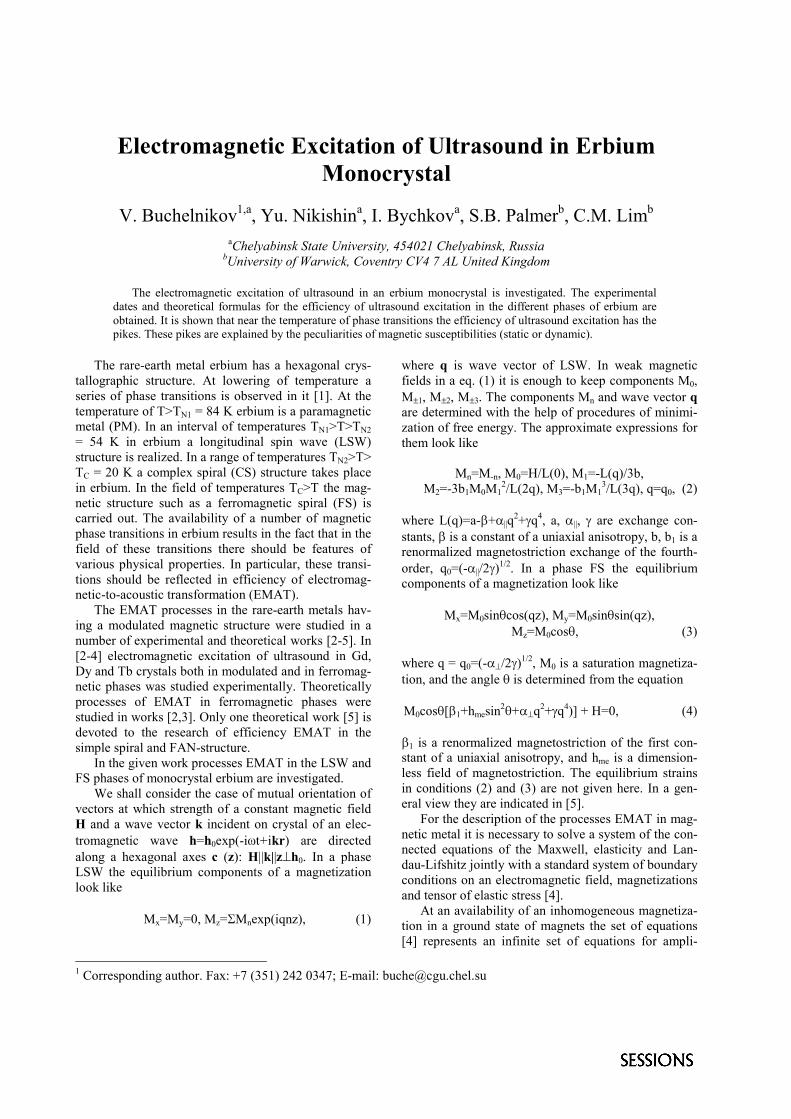
Electromagnetic Excitation of Ultrasound in ErbiumMonocrystal

V. Buchelnikov1,a, Yu. Nikishina, I. Bychkova, S.B. Palmerb, C.M. Limb

aChelyabinsk State University, 454021 Chelyabinsk, RussiabUniversity of Warwick, Coventry CV4 7 AL United Kingdom

The electromagnetic excitation of ultrasound in an erbium monocrystal is investigated. The experimentaldates and theoretical formulas for the efficiency of ultrasound excitation in the different phases of erbium areobtained. It is shown that near the temperature of phase transitions the efficiency of ultrasound excitation has thepikes. These pikes are explained by the peculiarities of magnetic susceptibilities (static or dynamic).

1 Corresponding author. Fax: +7 (351) 242 0347; E-mail: buche@cgu.chel.su

The rare-earth metal erbium has a hexagonal crys-tallographic structure. At lowering of temperature aseries of phase transitions is observed in it [1]. At thetemperature of T>TN1 = 84 K erbium is a paramagneticmetal (PM). In an interval of temperatures TN1>T>TN2= 54 K in erbium a longitudinal spin wave (LSW)structure is realized. In a range of temperatures TN2>T>TC = 20 K a complex spiral (CS) structure takes placein erbium. In the field of temperatures TC>T the mag-netic structure such as a ferromagnetic spiral (FS) iscarried out. The availability of a number of magneticphase transitions in erbium results in the fact that in thefield of these transitions there should be features ofvarious physical properties. In particular, these transi-tions should be reflected in efficiency of electromag-netic-to-acoustic transformation (EMAT).

The EMAT processes in the rare-earth metals hav-ing a modulated magnetic structure were studied in anumber of experimental and theoretical works [2-5]. In[2-4] electromagnetic excitation of ultrasound in Gd,Dy and Tb crystals both in modulated and in ferromag-netic phases was studied experimentally. Theoreticallyprocesses of EMAT in ferromagnetic phases werestudied in works [2,3]. Only one theoretical work [5] isdevoted to the research of efficiency EMAT in thesimple spiral and FAN-structure.

In the given work processes EMAT in the LSW andFS phases of monocrystal erbium are investigated.

We shall consider the case of mutual orientation ofvectors at which strength of a constant magnetic fieldH and a wave vector k incident on crystal of an elec-tromagnetic wave h=h0exp(-i�t+ikr) are directedalong a hexagonal axes c (z): H||k||z�h0. In a phaseLSW the equilibrium components of a magnetizationlook like

Mx=My=0, Mz=�Mnexp(iqnz), (1)

where q is wave vector of LSW. In weak magneticfields in a eq. (1) it is enough to keep components M0,M�1, M�2, M�3. The components Mn and wave vector qare determined with the help of procedures of minimi-zation of free energy. The approximate expressions forthem look like

Mn=M-n, M0=H/L(0), M1=-L(q)/3b,M2=-3b1M0M1

2/L(2q), M3=-b1M13/L(3q), q=q0, (2)

where L(q)=a-�+�||q2+�q4, a, �||, � are exchange con-stants, � is a constant of a uniaxial anisotropy, b, b1 is arenormalized magnetostriction exchange of the fourth-order, q0=(-�||/2�)1/2. In a phase FS the equilibriumcomponents of a magnetization look like

Mx=M0sin�cos(qz), My=M0sin�sin(qz),Mz=M0cos�, (3)

where q = q0=(-��/2�)1/2, M0 is a saturation magnetiza-tion, and the angle � is determined from the equation

M0cos�[�1+hmesin2�+��q2+�q4)] + H=0, (4)

�1 is a renormalized magnetostriction of the first con-stant of a uniaxial anisotropy, and hme is a dimension-less field of magnetostriction. The equilibrium strainsin conditions (2) and (3) are not given here. In a gen-eral view they are indicated in [5].

For the description of the processes EMAT in mag-netic metal it is necessary to solve a system of the con-nected equations of the Maxwell, elasticity and Lan-dau-Lifshitz jointly with a standard system of boundaryconditions on an electromagnetic field, magnetizationsand tensor of elastic stress [4].

At an availability of an inhomogeneous magnetiza-tion in a ground state of magnets the set of equations[4] represents an infinite set of equations for ampli-

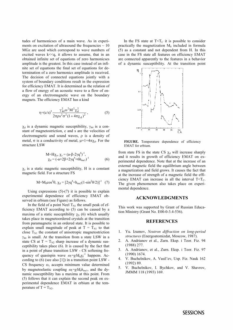
tudes of harmonicses of a main wave. As in experi-ments on excitation of ultrasound the frequencies ~ 10MGz are used which correspond to wave numbers ofexcited waves k<<q, it allows to assume, that in anobtained infinite set of equations of zero harmonicsesamplitude is the greatest. In this case instead of an infi-nite set of equations the final set of equations for de-termination of a zero harmonics amplitude is received.The decision of connected equations jointly with asystem of boundary conditions result in the expressionfor efficiency EMAT. It is determined as the relation ofa flow of energy of an acoustic wave to a flow of en-ergy of an electromagnetic wave on the boundarymagnets. The efficiency EMAT has a kind

�=(c/s)32

d22

2d

22244

)41(s2M

������

���, (5)

d is a dynamic magnetic susceptibility, �44 is a con-stant of magnetostriction, c and s are the velocities ofelectromagnetic and sound waves, is a density ofmetal, � is a conductivity of metal, �=1+4 d. For thestructure LSW

M=Hs, s = (a-�-2�q4)-1,d = (-a+2�+2�q4+6hme1)-1 (6)

s is a static magnetic susceptibility, H is a constantmagnetic field. For a structure FS

M=M0cos2�, d = [2�q4+hme2(1-sin2�/2)]-1 (7)

Using expressions (5)-(7) it is possible to explainexperimental dependence of efficiency EMAT ob-served in erbium (see Figure) as follows.

In the field of a point Neel TN1 the small peak of ef-ficiency EMAT according to (5) can be caused by amaxima of a static susceptibility S (6) which usuallytakes place in magnetoordered crystals at the transitionfrom paramagnetic in an ordered state. It is possible toexplain small magnitude of peak at T = TN1 to thatclose TN1 the constant of anisotropic magnetostriction�44 is small. At the transition from a state LSW in astate CS at T = TN2 sharp increase of a dynamic sus-ceptibility takes place (6). It is caused by the fact thatin a point of phase transition LSW - CS softening fre-quency of quasispin wave �1=gM0�d

-1 happens. Ac-cording to (6) (see also [1]) in a transition point LSW -CS frequency �1 accepts minimum value determinedby magnetoelastic coupling �1=gM0hme1, and the dy-namic susceptibility has a maxima at this point. From(5) follows that it can explain the second peak on ex-perimental dependence EMAT in erbium at the tem-perature of T = TN2.

In the FS state at T<TC it is possible to considerpractically the magnetization M0 included in formula(5) as a constant and not dependent from H. In thiscase in the FS state all features on efficiency EMATare connected apparently to the features in a behaviorof a dynamic susceptibility. At the transition point

from state FS in the state CS d will increase sharplyand it results in growth of efficiency EMAT on ex-perimental dependence. Note that at the increase of anexternal magnetic field the equilibrium angle betweena magnetization and field grows. It causes the fact thatat the increase of strength of a magnetic field the effi-ciency EMAT can increase in all the interval T<TC.The given phenomenon also takes place on experi-mental dependence.

ACKNOWLEDGMENTS

This work was supported by Grant of Russian Educa-tion Ministry (Grant No. E00-0-3.4-536).

REFERENCES

1. Yu. Izumov, Neutron diffraction on long-periodstructures (Energoatomizdat, Moscow, 1987).

2. A. Andrianov et al., Zurn. Eksp. i Teor. Fiz. 94(1988) 277.

3. A. Andrianov, et al., Zurn. Eksp. i Teor. Fiz. 97(1990) 1674.

4. V. Buchelnikov, A. Vasil’ev, Usp. Fiz. Nauk 162(1992) 89.

5. V. Buchelnikov, I. Bychkov, and V. Shavrov,JMMM 118 (1993) 169.

FIGURE. Temperature dependence of efficiencyEMAT for erbium.

Ultrasonic Gas Jet Waveguides for Air-coupled NDED.A. Hutchins, D.-W. Choi and D.R. Billson

School of Engineering, University of Warwick, Coventry CV4 7AL, UK

Studies have been performed of ultrasonic beams in gases, generated by a transducer placed along the axis of a gas jet. Thetransducers used were polymer-based electrostatic devices with a micromachined silicon backplate. The ultrasonic beams emittedfrom the devices in still air were compared to those in the presence of an axial gas jet, using either air or some other gas.Divergence of the beam was noted for an air jet, due to refraction effects. However, when the air was changed to one with alower sound velocity, such as carbon dioxide, the beam was contained within the gas jet, i.e. the gas jet itself was acting as awaveguide. This is an interesting effect, which could be used to increase the lateral resolution of air-coupled ultrasonic images,and could be used in turbulent environments.

INTRODUCTION

Air-coupled ultrasound is being used increasinglyas a method for materials inspection without contact1.In this technique, air is used as the coupling medium tothe sample. Although the acoustic impedancedifference between air and solid materials such asmetals and polymers is large, recent developments intransducer technology have made it possible for signalsto be transmitted through the solid material under test,using air as the coupling medium. The present paperinvestigates the possibility of transmitting ultrasonicsignals along a gas jet, which would act as a form ofwaveguide. Within this waveguide, the propagationcharacteristics can be controlled, so that improvedconditions for transmission could be obtained (e.g.increased directivity and lower attenuation). Suchchanges would be induced by differences in the gasflow velocity and temperature between the gas jet andits surroundings, which in turn lead to a difference inthe acoustic velocity.

The propagation of acoustic waves in a gas jet hasbeen studied extensively2. Acoustic refraction isobserved, as the sound velocity increases in thedirection of flow, and this flow decreases radiallyacross the jet. The result is divergence of the soundfield. In the present application, the aim is to use thegas jet as a propagation medium for an ultrasonicsignal, where confinement of the beam would be anadvantage. One way in which this might be achievedis to change the sound speed in the gas jet itself, so thatit is lower than the surrounding air into which it travels(e.g. by changing the gas or lowering the temperaturein the gas jet). The latter effect has been observed ataudible frequencies within a cold nitrogen gas jet2,where convergence towards the jet axis was seen. Thispaper extends the above research by studying theradiated ultrasonic field from a transducer placed

within the flow of a gas jet, and to determine whetheran effective waveguide can be obtained.

APPARATUS AND EXPERIMENT

Ultrasonic signals were generated using acapacitive transducer, a schematic diagram of which isshown in Figure 1.

FIGURE 1. Diagram of a capacitance transducer.

These transducers use a thin polymer membraneattracted against a machined metal or silicon backplate,which causes a layer of air to be trapped behind themembrane3. It is important in these devices that thebackplate surface features are well-controlled, so thatthe mechanical behaviour of the device can bepredicted. The present device contained amicromachined silicon backplate, against which wasplaced a 5�m thick Mylar polymer membrane, with agrounded metal coating on the outer surface.Frequencies of up to 1MHz could be generated with agood sensitivity. Metal springs were used to hold thetransducer within a polymer tube, at the end of whichan ogive nozzle was placed. The springs minimised

disruption to the air flow within the pipe due theirsmall flow cross-section. This was not crucial,however, due to the use of the ogive nozzle design, asthis tended to smooth out any turbulence caused by thetransducer casing. Both the ultrasonic beam and thegas jet were emitted into the surrounding air throughthis nozzle, so that the gas jet and the ultrasonic beamwere propagating along the same axis.

Spatial variations in both the ultrasonic field andthe gas flow velocity across two–dimensional sectionsthroughout the gas flow were measured, by scanningminiature ultrasonic receivers and flow velocitysensors respectively through the same sections of flow.Scanning was performed in a horizontal plane using anX–Y linear stage, driven by standard stepper motors.These were controlled using a Labview program and a2-axis programmable stepper motor driver unit. Thedata was then displayed on a Tektronix TDS540 digitaloscilloscope, and subsequently transferred to the PCfor storage and later analysis. The transducer within thepipe, and the scanning plane, were carefully alignedwith each other using a HeNe laser. Each scancommenced at the centre of the nozzle aperture as areference point for all scans, over typical distances of80mm axial (z) and 80mm radial (r). Typical scanswere performed by recording data at 1mm spatialintervals. A range of gases could be used for the gasjets, with an adjustable flow rate.

RESULTS AND DISCUSSION

The first experiments measured the ultrasonic fieldemitted from the nozzle, both before and after an air jetwas established. The results for a 5mm diameter ogivenozzle are shown in Figure 2 (a) and (b) respectively.

-5 0 50

5

10

15

-5 0 50

5

10

15

(a) (b)

FIGURE 2. Ultrasonic fields for transient excitation in (a)still air and (b) in an air jet with an exit velocity of 1.7 ms-1.

It can be observed that the introduction of air flowhas caused divergence of the ultrasonic beam, asexpected. The experiments were now repeated forair/helium and air/CO2 mixtures, where the ambientacoustic velocity will be respectively above and below

that of still air. (Note: the velocity in helium is~965ms-1, and ~260ms-1 in CO2). The results, shown inFigures 3 (a) and 3(b), indicate that helium leads toincreased divergence, but that the addition of CO2 leadsto a prominent waveguide effect4.

-5 0 50

5

10

15

-5 0 50

5

10

15

(a) (b)

FIGURE 3. Ultrasonic field for a gas jet containing (a) anair/helium mixture, and (b) an air/ CO2 mixture, both in a5:1 ratio by volume. The exit velocity was 2.0 ms-1.

CONCLUSIONS

The research has demonstrated that an ultrasonicsignal can be propagated along a gas jet, by mounting atransducer within the gas flow. The ogive nozzle actedto smooth the air flow, minimizing disturbance by thetransducer. Air flow was seen to increase ultrasonicbeam divergence, as expected. However, introducinggases with different sound speeds caused interestingeffects. Helium caused further divergence, whereasCO2 produced a well-collimated beam. This is thoughtto have many applications in air-coupled NDE.

ACKNOWLEDGEMENTS

This work was funded by grants from BG plc andthe Engineering and Physical Sciences ResearchCouncil (EPSRC).

REFERENCES

1. W.A. Grandia and C.M. Fortunko, Proc. 1995 IEEEUltrasonics Symp., 1, 697-709 (1995).

2. E. Grande, J. Acoust. Soc. Am., 38, 1063-1064 (1965).3. D.W.Schindel, D.A. Hutchins, L. Zou & M.Sayer, IEEE

Trans. Ultrason. Ferro. Freq. Cont. 42, 42–50 (1995).4. D.A. Hutchins, C.S. McIntyre, D.W. Choi, D.R. Billson

and T.J. Robertson, submitted to J. Acoust. Soc. Am.

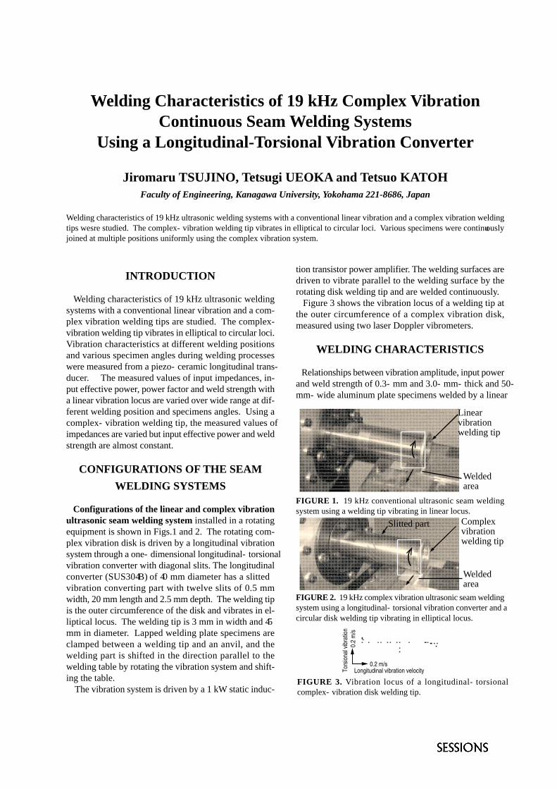
Welding Characteristics of 19 kHz Complex VibrationContinuous Seam Welding Systems

Using a Longitudinal-Torsional Vibration Converter

Jiromaru TSUJINO, Tetsugi UEOKA and Tetsuo KATOHFaculty of Engineering, Kanagawa University, Yokohama 221-8686, Japan

Welding characteristics of 19 kHz ultrasonic welding systems with a conventional linear vibration and a complex vibration weldingtips wesre studied. The complex-vibration welding tip vibrates in elliptical to circular loci. Various specimens were continuouslyjoined at multiple positions uniformly using the complex vibration system.

INTRODUCTION

Welding characteristics of 19 kHz ultrasonic weldingsystems with a conventional linear vibration and a com-plex vibration welding tips are studied. The complex-vibration welding tip vibrates in elliptical to circular loci.Vibration characteristics at different welding positionsand various specimen angles during welding processeswere measured from a piezo-ceramic longitudinal trans-ducer. The measured values of input impedances, in-put effective power, power factor and weld strength witha linear vibration locus are varied over wide range at dif-ferent welding position and specimens angles. Using acomplex-vibration welding tip, the measured values ofimpedances are varied but input effective power and weldstrength are almost constant.

CONFIGURATIONS OF THE SEAM

WELDING SYSTEMS

Configurations of the linear and complex vibrationultrasonic seam welding system installed in a rotatingequipment is shown in Figs.1 and 2. The rotating com-plex vibration disk is driven by a longitudinal vibrationsystem through a one-dimensional longitudinal-torsionalvibration converter with diagonal slits. The longitudinalconverter (SUS304B) of 40 mm diameter has a slittedvibration converting part with twelve slits of 0.5 mmwidth, 20 mm length and 2.5 mm depth. The welding tipis the outer circumference of the disk and vibrates in el-liptical locus. The welding tip is 3 mm in width and 45mm in diameter. Lapped welding plate specimens areclamped between a welding tip and an anvil, and thewelding part is shifted in the direction parallel to thewelding table by rotating the vibration system and shift-ing the table. The vibration system is driven by a 1 kW static induc-

tion transistor power amplifier. The welding surfaces aredriven to vibrate parallel to the welding surface by therotating disk welding tip and are welded continuously. Figure 3 shows the vibration locus of a welding tip atthe outer circumference of a complex vibration disk,measured using two laser Doppler vibrometers.

WELDING CHARACTERISTICS

Relationships between vibration amplitude, input powerand weld strength of 0.3-mm and 3.0-mm-thick and 50-mm-wide aluminum plate specimens welded by a linear

FIGURE 1. 19 kHz conventional ultrasonic seam weldingsystem using a welding tip vibrating in linear locus.

FIGURE 2. 19 kHz complex vibration ultrasonic seam weldingsystem using a longitudinal-torsional vibration converter and acircular disk welding tip vibrating in elliptical locus.

0.2 m/s

0.2

m/s

Longitudinal vibration velocityTors

iona

l vib

ratio

n

FIGURE 3. Vibration locus of a longitudinal-torsionalcomplex-vibration disk welding tip.

Slitted part Complexvibrationwelding tip

Linearvibrationwelding tip

Weldedarea

Weldedarea

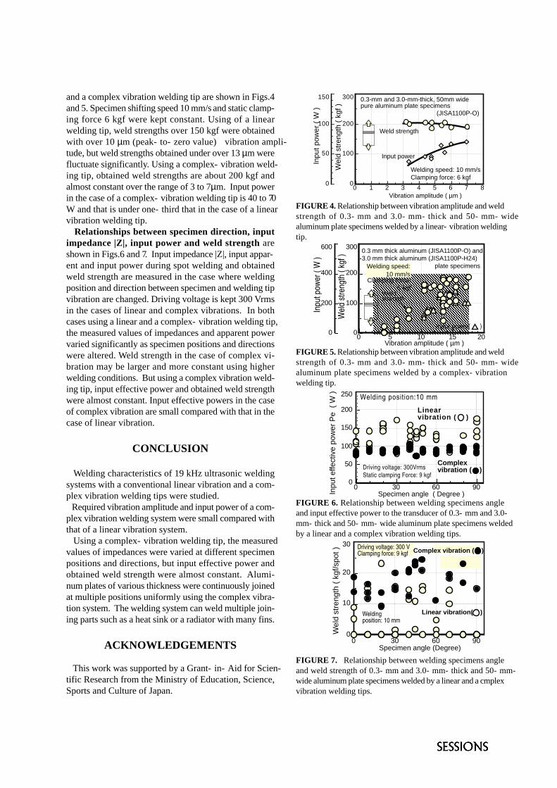
and a complex vibration welding tip are shown in Figs.4and 5. Specimen shifting speed 10 mm/s and static clamp-ing force 6 kgf were kept constant. Using of a linearwelding tip, weld strengths over 150 kgf were obtainedwith over 10 µm (peak-to-zero value) vibration ampli-tude, but weld strengths obtained under over 13 µm werefluctuate significantly. Using a complex-vibration weld-ing tip, obtained weld strengths are about 200 kgf andalmost constant over the range of 3 to 7 µm. Input powerin the case of a complex-vibration welding tip is 40 to 70W and that is under one-third that in the case of a linearvibration welding tip. Relationships between specimen direction, inputimpedance |Z|, input power and weld strength areshown in Figs.6 and 7. Input impedance |Z|, input appar-ent and input power during spot welding and obtainedweld strength are measured in the case where weldingposition and direction between specimen and welding tipvibration are changed. Driving voltage is kept 300 Vrmsin the cases of linear and complex vibrations. In bothcases using a linear and a complex-vibration welding tip,the measured values of impedances and apparent powervaried significantly as specimen positions and directionswere altered. Weld strength in the case of complex vi-bration may be larger and more constant using higherwelding conditions. But using a complex vibration weld-ing tip, input effective power and obtained weld strengthwere almost constant. Input effective powers in the caseof complex vibration are small compared with that in thecase of linear vibration.

CONCLUSION

Welding characteristics of 19 kHz ultrasonic weldingsystems with a conventional linear vibration and a com-plex vibration welding tips were studied. Required vibration amplitude and input power of a com-plex vibration welding system were small compared withthat of a linear vibration system. Using a complex-vibration welding tip, the measuredvalues of impedances were varied at different specimenpositions and directions, but input effective power andobtained weld strength were almost constant. Alumi-num plates of various thickness were continuously joinedat multiple positions uniformly using the complex vibra-tion system. The welding system can weld multiple join-ing parts such as a heat sink or a radiator with many fins.

ACKNOWLEDGEMENTS

This work was supported by a Grant-in-Aid for Scien-tific Research from the Ministry of Education, Science,Sports and Culture of Japan.

FIGURE 4. Relationship between vibration amplitude and weldstrength of 0.3-mm and 3.0-mm-thick and 50-mm-widealuminum plate specimens welded by a linear-vibration weldingtip.

FIGURE 5. Relationship between vibration amplitude and weldstrength of 0.3-mm and 3.0-mm-thick and 50-mm-widealuminum plate specimens welded by a complex-vibrationwelding tip.

FIGURE 6. Relationship between welding specimens angleand input effective power to the transducer of 0.3-mm and 3.0-mm-thick and 50-mm-wide aluminum plate specimens weldedby a linear and a complex vibration welding tips.

FIGURE 7. Relationship between welding specimens angleand weld strength of 0.3-mm and 3.0-mm-thick and 50-mm-wide aluminum plate specimens welded by a linear and a cmplexvibration welding tips.

0

50

100

150

0

100

200

300

0 1 2 3 4 5 6 7 8Vibration amplitude ( µm )

0.3-mm and 3.0-mm-thick, 50mm widepure aluminum plate specimens

Welding speed: 10 mm/sClamping force: 6 kgf

Weld strength

Input power

(JISA1100P-O)

Wel

d st

reng

th (

kgf

)

Inpu

t pow

er (

W )

0

200

400

600

0

100

200

300

0 5 10 15 20Vibration amplitude ( µm )

Input power ( )

Weld strength

0.3 mm thick aluminum (JISA1100P-O) and3.0 mm thick aluminum (JISA1100P-H24)

plate specimens

Clamping force:

6 kgf

Welding speed:10 mm/s

Inpu

t pow

er (

W )

Wel

d st

reng

th (

kgf )

0

50

100

150

200

250

0 30 60 90

Welding position:10 mm

Linearvibration ( )

Inpu

t effe

ctiv

e po

wer

Pe

( W

)

Driving voltage: 300VrmsStatic clamping Force: 9 kgf

Specimen angle ( Degree )

Complexvibration ( )

0

10

20

30

0 30 60 90Specimen angle (Degree)

Weldingposition: 10 mm

Driving voltage: 300 VClamping force: 9 kgf

Linear vibration( )

Wel

d st

reng

th (

kgf

/spo

t ) Complex vibration ( )

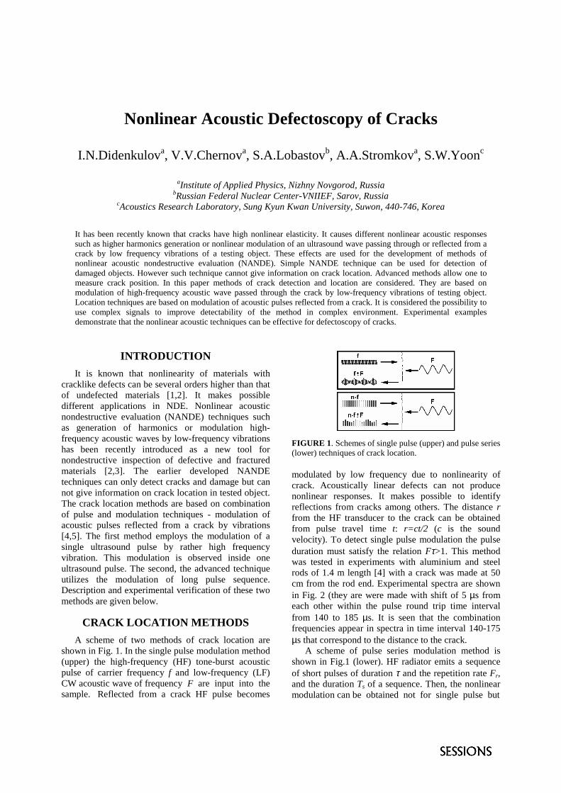
Nonlinear Acoustic Defectoscopy of Cracks

I.N.Didenkulova, V.V.Chernova, S.A.Lobastovb, A.A.Stromkova, S.W.Yoonc

aInstitute of Applied Physics, Nizhny Novgorod, RussiabRussian Federal Nuclear Center-VNIIEF, Sarov, Russia

cAcoustics Research Laboratory, Sung Kyun Kwan University, Suwon, 440-746, Korea

It has been recently known that cracks have high nonlinear elasticity. It causes different nonlinear acoustic responsessuch as higher harmonics generation or nonlinear modulation of an ultrasound wave passing through or reflected from acrack by low frequency vibrations of a testing object. These effects are used for the development of methods ofnonlinear acoustic nondestructive evaluation (NANDE). Simple NANDE technique can be used for detection ofdamaged objects. However such technique cannot give information on crack location. Advanced methods allow one tomeasure crack position. In this paper methods of crack detection and location are considered. They are based onmodulation of high-frequency acoustic wave passed through the crack by low-frequency vibrations of testing object.Location techniques are based on modulation of acoustic pulses reflected from a crack. It is considered the possibility touse complex signals to improve detectability of the method in complex environment. Experimental examplesdemonstrate that the nonlinear acoustic techniques can be effective for defectoscopy of cracks.

INTRODUCTIONIt is known that nonlinearity of materials with

cracklike defects can be several orders higher than thatof undefected materials [1,2]. It makes possibledifferent applications in NDE. Nonlinear acousticnondestructive evaluation (NANDE) techniques suchas generation of harmonics or modulation high-frequency acoustic waves by low-frequency vibrationshas been recently introduced as a new tool fornondestructive inspection of defective and fracturedmaterials [2,3]. The earlier developed NANDEtechniques can only detect cracks and damage but cannot give information on crack location in tested object.The crack location methods are based on combinationof pulse and modulation techniques - modulation ofacoustic pulses reflected from a crack by vibrations[4,5]. The first method employs the modulation of asingle ultrasound pulse by rather high frequencyvibration. This modulation is observed inside oneultrasound pulse. The second, the advanced techniqueutilizes the modulation of long pulse sequence.Description and experimental verification of these twomethods are given below.

CRACK LOCATION METHODSA scheme of two methods of crack location are

shown in Fig. 1. In the single pulse modulation method(upper) the high-frequency (HF) tone-burst acousticpulse of carrier frequency f and low-frequency (LF)CW acoustic wave of frequency F are input into thesample. Reflected from a crack HF pulse becomes

FIGURE 1. Schemes of single pulse (upper) and pulse series(lower) techniques of crack location.

modulated by low frequency due to nonlinearity ofcrack. Acoustically linear defects can not producenonlinear responses. It makes possible to identifyreflections from cracks among others. The distance rfrom the HF transducer to the crack can be obtainedfrom pulse travel time t: r=ct/2 (c is the soundvelocity). To detect single pulse modulation the pulseduration must satisfy the relation Fτ>1. This methodwas tested in experiments with aluminium and steelrods of 1.4 m length [4] with a crack was made at 50cm from the rod end. Experimental spectra are shownin Fig. 2 (they are were made with shift of 5 µs fromeach other within the pulse round trip time intervalfrom 140 to 185 µs. It is seen that the combinationfrequencies appear in spectra in time interval 140-175µs that correspond to the distance to the crack.

A scheme of pulse series modulation method isshown in Fig.1 (lower). HF radiator emits a sequenceof short pulses of duration τ and the repetition rate Fr,and the duration Ts of a sequence. Then, the nonlinearmodulation can be obtained not for single pulse but

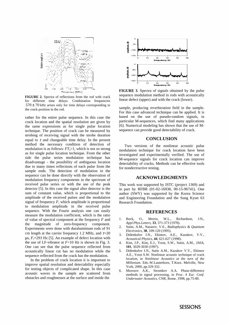
FIGURE 2. Spectra of reflections from the rod with crackfor different time delays. Combination frequencies

70570 ± kHz arises only for time delays corresponding tothe crack position in the rod.

rather for the entire pulse sequence. In this case thecrack location and the spatial resolution are given bythe same expressions as for single pulse locationtechnique. The position of crack can be measured bystrobing of receiving signal with the strobe durationequal to τ and changeable time delay. In the presentmethod the necessary condition of detection ofmodulation is as follows: FTs>1, which is not so strongas for single pulse location technique. From the otherside the pulse series modulation technique hasdisadvantage - the possibility of ambiguous locationdue to many times reflections of each pulse from thesample ends. The detection of modulation in thesequence can be done directly with the observation ofmodulation frequency components in the spectrum ofreceived pulse series or with the use of the peakdetector [5]. In this case the signal after detector is thesum of constant value, which is proportional to theamplitude of the received pulses and the modulationsignal of frequency F, which amplitude is proportionalto modulation amplitude in the received pulsesequence. With the Fourie analysis one can easilymeasure the modulation coefficient, which is the ratioof value of spectral component at the frequency F andthe magnitude of zero-frequency component.Experiments were done with duraluminium rods of 91cm length at the carrier frequency 1.2 MHz, and τ=20µs, Fr=293 Hz [5]. An example of defect location withthe use of LF-vibrator at F=10 Hz is shown in Fig. 3.One can see that the pulse sequence reflected fromacoustically linear cut has no modulation while thesequence reflected from the crack has the modulation.

In the problem of crack location it is important toimprove spatial resolution and detectability especiallyfor testing objects of complicated shape. In this caseacoustic waves in the sample are scattered fromobstacles and roughnesses at the surface and inside the

FIGURE 3. Spectra of signals obtained by the pulsesequence modulation method in rods with acousticallylinear defect (upper) and with the crack (lower).

sample, producing reverberation field in the sample.For this case advanced technique can be applied. It isbased on the use of pseudo-random signals, inparticular M-sequences, which find many applications[6]. Numerical modeling has shown that the use of M-sequence can provide good detectability of crack.

CONCLUSIONTwo versions of the nonlinear acoustic pulse

modulation technique for crack location have beeninvestigated and experimentally verified. The use ofM-sequence signals for crack location can improvedetectability of cracks. Methods can be effective toolsfor nondectructive testing.

ACKNOWLEDGMENTSThis work was supported by ISTC (project 1369) andin part by RFBR (01-02-16938, 00-15-96741). Oneauthor (SWY) was supported by the Korea Scienceand Engineering Foundation and the Sung Kyun 63Research Foundation.

REFERENCES1. Buck, O., Morris, W.L., Richardson, J.N.,

Appl.Phys.Letters, 33, 371-373 (1978).2. Sutin, A.M., Nazarov, V.E., Radiophysics & Quantum

Electronics, 38, 109-120 (1995).3. Didenkulov I.N., Ekimov, A.E., Kazakov, V.V.,

Acoustical Physics, 44, 621-627 (1998).4. Kim, J.P., Kim, E.J., Yoon, S.W., Sutin, A.M., JASA,

101, 3029-3030 (1997).5. Didenkulov I.N., Sutin A.M., Kazakov V.V., Ekimov

A.E., Yoon S.W. Nonlinear acoustic technique of cracklocation, in Nonlinear Acoustics at the turn of theMillenium. Eds.:W.Lauterborn, T.Kurz. Melville, NewYork, 2000, pp.329-332.

6. Morozov A.K., Stromkov A.A. Phase-differencemethods in signal processing, in Proc. 4 Eur. Conf.Underwater Acoustics, CNR, Rome, 1998, pp.75-80.