Non-gaussian dynamic bayesian modelling for panel data

MPRAMunich Personal RePEc Archive

Non-Gaussian dynamic Bayesianmodelling for panel data

Miguel A. Juarez and Mark F. J. Steel

July 2006

Online at http://mpra.ub.uni-muenchen.de/450/MPRA Paper No. 450, posted 15. October 2006

http://mpra.ub.uni-muenchen.de/

http://mpra.ub.uni-muenchen.de/450/

Non-Gaussian Dynamic Bayesian Modelling for

Panel Data

Miguel A. Juárez and Mark F. J. Steel∗

University of Warwick

Abstract

A first order autoregressive non-Gaussian model for analysing panel data is proposed.

The main feature is that the model is able to accommodate fat tails and also skewness,

thus allowing for outliers and asymmetries. The modelling approach is to gain suffi-

cient flexibility, without sacrificing interpretability and computational ease. The model

incorporates individual effects and we pay specific attention to the elicitation of the prior.

As the prior structure chosen is not proper, we derive conditions for the existence of

the posterior. By considering a model with individual dynamic parameters we are also

able to formally test whether the dynamic behaviour is common to all units in the panel.

The methodology is illustrated with two applications involving earnings data and one on

growth of countries.

JEL Classification: C11; C23.

Keywords: autoregressive modelling; growth convergence; individual effects; labour

earnings; prior elicitation; posterior existence; skewed distributions.

1 Introduction

Autoregressive models are used extensively in the analysis of panel or longitudinal data

(Arellano, 2003; Baltagi, 2001; Hsiao and Pesaran, 2004; Liu and Tiao, 1980; Mátyás and

Sevestre, 1995; Sáfadi and Morettin, 2003). In this paper we will assume that the data

available y = yi t form a (possibly unbalanced) panel of i = 1, . . . ,m individuals for each

of which we have Ti consecutive observations, and focus on the first order autoregressive

model:

yi t = βi (1− α) + α yi t−1 + λ−12εi t , (1)

∗Corresponding author: Mark Steel, University of Warwick, Department of Statistics, CV4 7AL, Coventry,

UK. Email: [email protected]

1

CRiSM Paper No. 06-05, www.warwick.ac.uk/go/crism

2 2. The models

where the errors εi t are independent and identically distributed (iid) random quantities cen-

tred at zero with unit precision, and α is the parameter governing the dynamic behaviour

of the panel. The intercepts β = β1, . . . , βm are often called individual effects. It is also

assumed that the process is stationary, i.e. |α| < 1.

The common approach is to assume that the error term in (1) is standard Gaussian,

εi t ∼ N (εi t | 0,1). From a Bayesian perspective, which will be pursued in this paper, prior

distributions must be specified for the model parameters, α,β, λ, and any parameters index-

ing the error distribution. Then, inference is carried out using numerical techniques, usually

Markov chain Monte Carlo (MCMC). See e.g. Chib and Greenberg (1994); Nandram and

Petruccelli (1997); Wang and Ghosh (2002). To account for tail behaviour heavier than Nor-

mal, a useful approach is to specify a Student-tν distribution for the errors, with ν degrees of

freedom (often fixed at a small value) and to incorporate this into the sampler through a scale

mixture of Normals representation of the Student (augmenting with the mixing variables).

In order to achieve more flexibility, Hirano (2002) proposes a semiparametric approach,

with a nonparametric distribution on εit using a Dirichlet process prior. However, such a fully

nonparametric approach sacrifices interpretability and computational ease for the sake of

flexibility. Here we propose a flexible, yet fully parametric, framework, which allows us to

fully maintain control of the properties of the error distribution and facilitates computation,

interpretation, communication and testing.

Section 2 describes the models and the prior elicitation we propose, and provides con-

ditions for posterior propriety. These models are used in Section 3 in the context of three

applications: two involving earnings data (regional averages and individual earnings) and

one on GDP growth of countries. A final section concludes.

2 The models

The Student-tν model described briefly above has been used successfully in a number of ap-

plications. However, asymmetries are often found in real data which this formulation cannot

account for. Also, it seems sensible to let the data determine the tail behaviour, i.e. not to fix

ν in advance but estimate it along with the rest of the parameters.

There are a number of different classes of distributions for modelling unimodal skewed

data, and the most common approach is to modify an originally symmetric distribution. The

most pervasive mechanism is the hidden truncation idea (Arnold and Beaver, 2002), which

underlies the skew-Normal distribution introduced in Azzalini (1985) and is applied to (mul-

tivariate) Student-t distributions in Azzalini and Capitanio (2003). An alternative class of

skewed t distributions was proposed in Jones and Faddy (2003). Arnold and Beaver (2002)

and Genton (2004) present an overview of these and other approaches.


2. The models 3

Fernández and Steel (1998) introduced an alternative way of skewing univariate distribu-

tions, namely by scaling a symmetric distribution (around the origin) by reciprocal weights.

We will use these families of distributions in the sequel for a number of reasons: their param-

eters separately control for location, scale, skewness and tail behaviour, with the skewness

parameter being a simple transformation of an interpretable skewness measure, they are

easy to use, and they allow for any amount of skewness at either side of the mode.

Formally, Fernández and Steel (1998) consider a unimodal probability density function f ,

symmetric around zero, such that f (s) = f (|s|) and define the skew version of f , indexed by

γ ∈ R+, as

S f (s | γ) =2

γ + γ−1

[f (sγ) I(−∞,0](s) + f (sγ−1) I(0,∞)(s)

]. (2)

This skew version obviously does not have zero mean (for γ , 1), but still has a unique mode

at zero. Further, γ controls the amount of skewness (in particular, the relative amount of

probability mass to the right of the mode) given that

ϕ = γ2 =P[s> 0 | γ]P[s< 0 | γ]

.

Clearly, S f (s | γ) = S f (−s | 1/γ), so that γ > 1 and 1/γ introduce the same amount of right

and left skewness, respectively. By contrasting (2) with the original symmetric distribution

(the special case when γ = 1), we can test for symmetry.

In particular, we will focus on the skew versions of the Normal and Student-tν (or t) distri-

butions, leading to

SN (ε | γ) =2

γ + γ−1

√1

2πexp

[−1

2ε2

(γ2 I(−∞,0](ε) + γ−2 1(0,∞)(ε)

)], (3)

and

Skt (ε | γ, ν) =2

γ + γ−1

Γ[(ν + 1)/2]Γ[ν/2]

√1ν π

[1 +

1νε2

(γ2 I(−∞,0](ε) + γ−2 1(0,∞)(ε)

)]− ν+12

. (4)

Thus, we will use (1) with εi t distributed according to (3) or (4), for unit i = 1, . . . ,m, and

with T1, . . . ,Tm consecutive measurements in time. This parameterisation allows for a clear

interpretation of α as the parameter governing the dynamics of the panel, λ as driving the

precision in the measurements and βi as an individual location (level) or “individual effect”. In

addition, γ will control the skewness and, in the case of (4), ν determines the tail behaviour.

Since the error distributions have a mode at zero, individual effects are interpreted as the

corresponding modes. Further, these are assumed to be related according to

βi ∼ N (βi | β, τ) , (5)


4 2.1. The prior

which is a commonly used random effects specification, found e.g. in Liu and Tiao (1980),

Nandram and Petruccelli (1997) and Gelman (2006), where β is a common mean and τ the

precision. Within a Bayesian framework, (5) is merely a hierarchical specification of the prior

on the βi ’s. Also, we assume that the initial observed value for individual i is yi 0, on which we

condition throughout, and that the process started a long time ago.

2.1 The prior

For the full skew-t model we will specify a prior of the product form

π(α, β, τ, λ, γ, ν) = π(α)π(β)π(τ)π(λ)π(γ)π(ν) . (6)

Prior for (β, λ):

As we do not want to include strong prior beliefs, we will use the standard “diffuse” prior

for the individual effects’ mean β and for the observational precision, λ

π(β)π(λ) ∝ λ−1 . (7)

Prior for τ :

It is well known that a flat prior on the log of the precision in (5), i.e. π(τ) ∝ τ−1, will yield an

improper posterior (Hill, 1965; Sun et al., 2001). Gelman (2006) analyses this problem in the

context of hierarchical Gaussian models and proposes alternative distributions. Fernández

et al. (1997) give conditions under which the posterior is proper in the context of panel data

with unobserved heterogeneity in the location.

Here, we propose to elicit a proper prior, π(τ), centred at a value τ0. Specifically, we will

use a Gamma distribution with mode at τ0 (for aτ > 1) and use the shape parameter aτ to

control its spread, i.e. τ ∼ Ga (aτ, (aτ − 1)/τ0) or

π (τ | aτ, τ0) =

[(aτ − 1)/τ0

]aτ

Γ[aτ]τaτ−1 exp

[−(aτ − 1)

τ0τ]. (8)

Alternative forms for this prior are easily accommodated within the sampler, given that this will

only affect the conditional distribution on β, τ. As stated above, using the “noninformative”

prior on τ with density proportional to τ−1 would lead to an improper posterior. One com-

mon choice is to use the conditionally-conjugate prior in (8), set its mean at one (i.e. make

τ0 = (aτ − 1)/aτ) and then fix aτ at a value close to zero, in order to let its dispersion grow


2.1. The prior 5

(Spiegelhalter et al., 2004) and to approximate the noninformative prior mentioned above.

This specification allocates a lot of prior mass to low values of the precision. Gelman (2006)

argues that the resulting posterior can be quite sensitive to the particular choice of (small) aτif the data allow mass for τ close to zero.

Therefore, we take aτ = 2 which avoids a lot of prior mass close to zero and we calibrate

the prior to the scaling of the data by choosing the mode τ0 equal to c/s2β, where s2

β is

the (between-group) sample variance of the group means and c > 1 to account for the

influence of the within-group variation. We take c = 2 in our examples, which works well.

This dependence of the prior on a (fairly minor) aspect of the data is inevitable, if we wish

to avoid inadvertently informative priors and make sure that the prior information is never

greatly at odds with the data. However, the fairly small value of aτ (which is combined with

m/2 in the conditional posterior) means that the prior is still relatively vague and prior mass

is spread over a wide range of (reasonable) values.

Prior for γ:

To specify a prior for γ we focus on a more readily interpretable quantity, namely the

(scale-free) amount of skewness, AG, measured as in Arnold and Groeneveld (1995) by one

minus twice the probability mass left of the mode. In the case of the skew family defined

by (2) this is simply a one-to-one function of the relative amount of mass to the right of the

mode, ϕ = γ2

AG =ϕ − 1ϕ + 1

.

This means that we are able to derive equivalent priors, starting from either parameterisa-

tion of the skewness parameter. Clearly, −1 < AG < 1, with negative (positive) values

corresponding to left (right) skewness and AG = 0 for the original, symmetric model.

We propose a Beta prior distribution on AG, rescaled to (-1,1),

π (AG | a,b) =21−a−b

B(a,b)(1 + AG)a−1(1− AG)b−1 a,b > 0 ,

thus implying

π (ϕ | a,b) =1

B(a,b)ϕa−1 (1 + ϕ)−(a+b) ,

an inverted Beta distribution with parameters (a,b,1) (Zellner, 1971, p. 376), which, in turn,

implies that abϕ follows a Snedecor F(2a,2b) distribution with (2a,2b) degrees of freedom. In

particular, setting a = b implies symmetry in the distribution for AG, which we think is sen-

sible in the absence of strong prior beliefs. Thus, ϕ ∼ F(2a,2a) and, therefore, P[ϕ < x] =

P[ϕ > 1/x], which extends directly to the parameterisation on γ, addressing in a natural way

the symmetry between γ and γ−1 described in the discussion following (2). Figure 1 depicts

the implied prior on γ for different values of the hyperparameter a.


6 2.1. The prior

1 2 3 4 5

0.25

0.5

0.75

1

1.25

1.5

1.75

γ

a = 0.5

a = 1

a = 3

a = 10

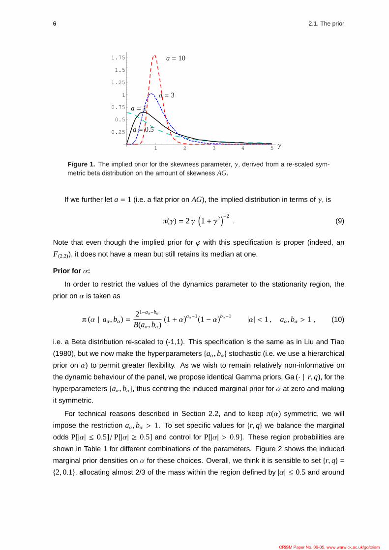
Figure 1. The implied prior for the skewness parameter, γ, derived from a re-scaled sym-metric beta distribution on the amount of skewness AG.

If we further let a = 1 (i.e. a flat prior on AG), the implied distribution in terms of γ, is

π(γ) = 2γ(1 + γ2

)−2. (9)

Note that even though the implied prior for ϕ with this specification is proper (indeed, an

F(2,2)), it does not have a mean but still retains its median at one.

Prior for α:

In order to restrict the values of the dynamics parameter to the stationarity region, the

prior on α is taken as

π (α | aα,bα) =21−aα−bα

B(aα,bα)(1 + α

)aα−1(1− α)bα−1 |α| < 1 , aα,bα > 1 , (10)

i.e. a Beta distribution re-scaled to (-1,1). This specification is the same as in Liu and Tiao

(1980), but we now make the hyperparameters aα,bα stochastic (i.e. we use a hierarchical

prior on α) to permit greater flexibility. As we wish to remain relatively non-informative on

the dynamic behaviour of the panel, we propose identical Gamma priors, Ga (· | r,q), for the

hyperparameters aα,bα, thus centring the induced marginal prior for α at zero and making

it symmetric.

For technical reasons described in Section 2.2, and to keep π(α) symmetric, we will

impose the restriction aα,bα > 1. To set specific values for r,q we balance the marginal

odds P[|α| ≤ 0.5]/P[|α| ≥ 0.5] and control for P[|α| > 0.9]. These region probabilities are

shown in Table 1 for different combinations of the parameters. Figure 2 shows the induced

marginal prior densities on α for these choices. Overall, we think it is sensible to set r,q =

2,0.1, allocating almost 2/3 of the mass within the region defined by |α| ≤ 0.5 and around


2.1. The prior 7

-1 -0.5 0.5 1

0.2

0.4

0.6

0.8

1(5,0.5)

(2,0.1)

(1,1)

(0.1,0.1)

α

Figure 2. Induced marginal priors for α, with Gamma hyperpriors Ga (· | r,q), and differentcombinations of r, q.

1/40 to the region where |α| ≥ 0.9. Therefore, we will use

π(aα) ∝ aα e−0.1aα , aα > 1 and π(bα) ∝ bα e−0.1bα , bα > 1 . (11)

Table 1. Induced marginal prior probabilities for α with Gamma,Ga (· | r, q), hyperpriors.

r,q (5,0.5) (2,0.1) (1,1) (0.1,0.1)P[|α| ≤ 0.5

]0.805 0.658 0.575 0.495

P[|α| ≥ 0.9

]0.004 0.026 0.056 0.085

Prior for ν:

Finally, for the (skew)-t model, we specify a Gamma(2,0.1) prior for the degrees of free-

dom, given by

π(ν) =ν

100e−ν/10 . (12)

This distribution assigns some mass to large values of ν (virtually implying Normality) as well

as to small values of the degrees of freedom, thus also allowing for thicker tails.

Priors for restrictions of the skew-t model (i.e. Normal, skew-Normal or Student-tν mod-

els) are obtained by deleting the corresponding irrelevant factors in (6).

Once data become available, (1) defines the likelihood which, using the scale mixture of

normals representation for the skew-t model, becomes

l(α,β, γ, λ,ω, ν, aα,bα) ∝ λT2[(ν/2

)ν/2Γ[ν/2]

]T m∏

i=1

Ti∏

t=1

ων+12 −1

i t

[21−aα−bα

B(aα,bα)(1+α

)aα−1(1−α)bα−1]×

[2

γ + γ−1

]Texp

[−1

2

m∑

i=1

Ti∑

t=1

ωi t

(ν + ε2

i t

(γ2 I(−∞,0](εi t) + γ−2 I(0,∞)(εi t)

))],


8 2.2. Propriety of the posterior

where ω = ωi t , i = 1, . . . ,m, t = 1, . . . ,Ti and the ωi t are iid, Gamma(ν/2, ν/2) distributed

mixing parameters, εi t = λ1/2(yi t − βi(1 − α) − α yi t−1

), and T =

∑mi=1 Ti , the total available

observations. This will be combined with the prior structure defined by (6) through (12).

2.2 Propriety of the posterior

Note that (7) makes the joint prior improper. The following theorem states a sufficient condi-

tion under which the resulting posterior is proper (i.e. well-defined as described in Fernández

et al., 1997). The proof is deferred to Appendix A.

Theorem 1.

Consider the Bayesian model defined by (1) (with either (3) or (4)), (5) and (6) through (12).

If T > m+ 1, then the joint posterior is proper .

As will be clear from the proof in the Appendix, the condition bα > 1 in (11) is important in

avoiding non-integrability due to the implied prior on βi(1− α) exploding as α → 1. We also

restrict aα > 1, in order to maintain symmetry on the induced prior for α.

The condition in Theorem 1 is very mild and trivial to check. Indeed, for example, as long

as Ti ≥ 1 with strict inequality for at least two units, the posterior will be proper.

2.3 A model with individual dynamics

In the next section we will analyse three data sets: one comprising average earnings in

14 metropolitan areas (Liu and Tiao, 1980), another with annual labour earnings of young

male household heads (Hirano, 2002) and the third one on GDP of 25 OECD countries. In

these studies, panels were formed not necessarily according to statistical criteria, but rather

geographical, demographical or political affinity, thus we think is sensible to verify whether

the dynamic properties should indeed be pooled. We feel this situation is likely to occur in

practice, so we entertain the “non-pooled” version of (1),

yi t = βi(1− αi) + αiyi t−1 + λ−12εi t , (13)

with individual dynamics parameters αi , i = 1, . . . ,m arising independently from the same

distribution (10). In order to make the comparison fair, the same prior structure and specifi-

cations for the error term εi t will be maintained.

We have a similar result for posterior existence, with the proof sketched in Appendix A.


3. Applications 9

Theorem 2.

Consider the Bayesian model defined by (13) (with either (3) or (4)), (5) and (6) through

(12). If T > 2m, then the joint posterior is proper .

This sufficient condition is somewhat more demanding than the one in Theorem 1, but is

still straightforward to check and quite easily satisfied in practice. If we have more than two

observations per individual on average, we are sure that the posterior exists.

3 Applications

Throughout, we will use the pooled model in (1) and the non-pooled model in (13), each with

the Normal (N), Student-tν (t), skew-Normal (SN; see (3)) and Skew-t (Skt; see (4)) error

distributions. As the posteriors are not of a known form, we implement (Metropolis-Hastings

within Gibbs) MCMC samplers to estimate the parameters. Details of the samplers used as

well as the Matlab code for implementing them are available upon request.

The MCMC samplers were ran for 1.7 × 105 repetitions, dropping the first 2 × 104 (the

burn-in) and then recording every tenth draw, thus ending up with chains of length 15,000.

The parameters of the proposal Metropolis-Hastings distributions were tuned as to achieve

acceptance rates of around 1/3. We will use the formal tool of Bayes factor (BF) to compare

alternative models, calculating the required marginal likelihoods with the method of Newton

and Raftery (1994), with their δ = 0.1. As a check on the numerical accuracy of the latter

method, we also compute Bayes factors through the Savage-Dickey density ratios (Verdinelli

and Wasserman, 1995), where this is feasible. We have successfully used the Bayesian

models and algorithms on two simulated panels (not reported): one set of pooled data and

the other non-pooled.

3.1 Regional average earnings

The data, described in Liu and Tiao (1980), consist of yearly averages of the hourly earn-

ings of production workers within each of 14 metropolitan areas in California (transformed to

growth rates). Each of the series ends in 1977 but have different beginnings, the longest be-

ginning in 1945 and the shortest in 1963. This data set has also been analysed by Nandram

and Petruccelli (1997).

Table 2 shows the log BF in favour of the Normal model with common dynamics. Thus,

negative numbers indicate support for the alternative model in question.1 Our model com-

1For example, the BF for the Normal model versus the skew-Normal, both with common dynamics, isexp(−8.04) = 0.0003. This means that, with unitary prior odds, the posterior odds are more than 3000 toone in favour of the skew-Normal model.


10 3.1. Regional average earnings

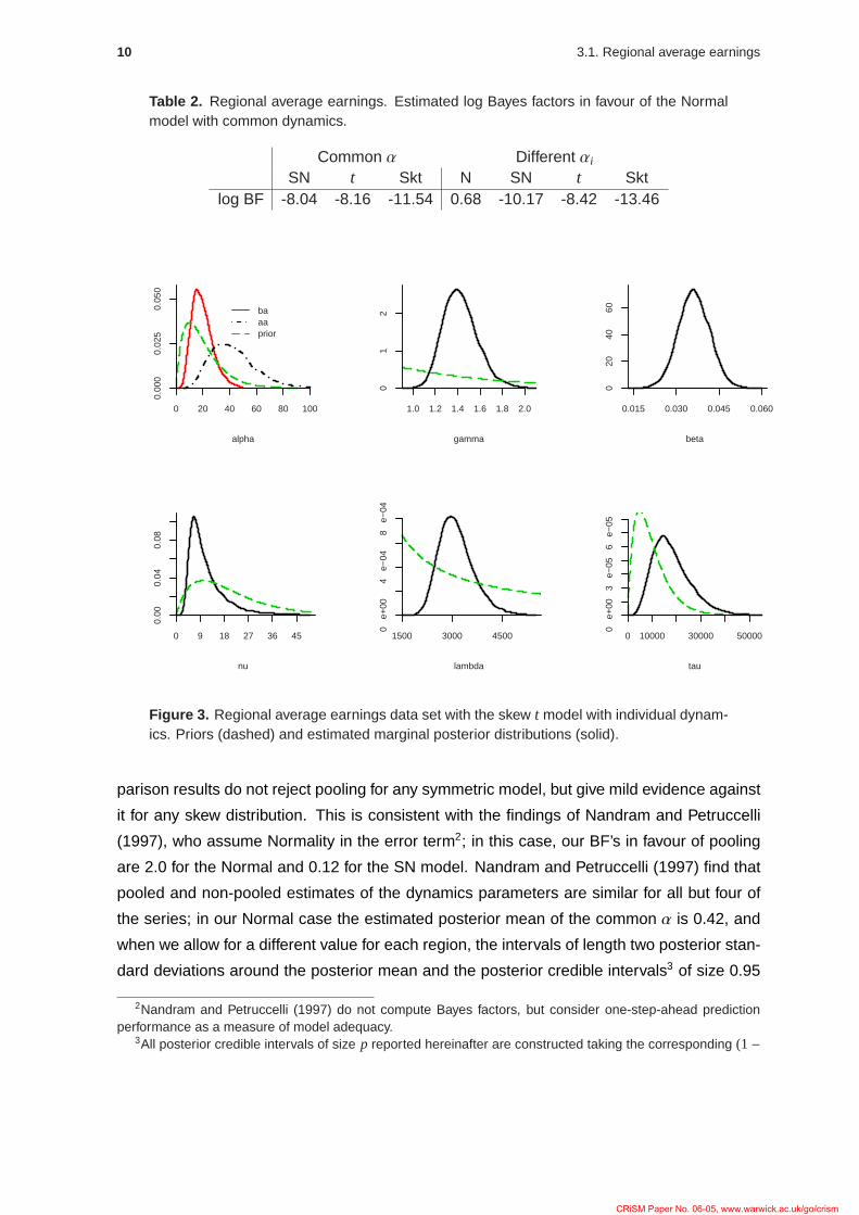
Table 2. Regional average earnings. Estimated log Bayes factors in favour of the Normalmodel with common dynamics.

Common α Different αi

SN t Skt N SN t Sktlog BF -8.04 -8.16 -11.54 0.68 -10.17 -8.42 -13.46

alpha

baaaprior

0 20 40 60 80 100

0.00

00.

025

0.05

0

gamma

1.0 1.2 1.4 1.6 1.8 2.0

01

2

beta

0.015 0.030 0.045 0.060

020

4060

nu

0 9 18 27 36 45

0.00

0.04

0.08

lambda

1500 3000 4500

0 e

+00

4 e

−04

8 e

−04

tau

0 10000 30000 50000

0 e

+00

3 e

−05

6 e

−05

Figure 3. Regional average earnings data set with the skew t model with individual dynam-ics. Priors (dashed) and estimated marginal posterior distributions (solid).

parison results do not reject pooling for any symmetric model, but give mild evidence against

it for any skew distribution. This is consistent with the findings of Nandram and Petruccelli

(1997), who assume Normality in the error term2; in this case, our BF’s in favour of pooling

are 2.0 for the Normal and 0.12 for the SN model. Nandram and Petruccelli (1997) find that

pooled and non-pooled estimates of the dynamics parameters are similar for all but four of

the series; in our Normal case the estimated posterior mean of the common α is 0.42, and

when we allow for a different value for each region, the intervals of length two posterior stan-

dard deviations around the posterior mean and the posterior credible intervals3 of size 0.95

2Nandram and Petruccelli (1997) do not compute Bayes factors, but consider one-step-ahead predictionperformance as a measure of model adequacy.

3All posterior credible intervals of size p reported hereinafter are constructed taking the corresponding (1−


3.2. Individual labour earnings data 11

for each region contain 0.42.

In the modelling scenario with common dynamics, the BF does not distinguish between

the SN and the t models. This could indicate that the model uses heavy tails to account

for asymmetry when the latter feature is not introduced in the model and vice versa. This

interpretation is corroborated by the fact that if the model only includes one of those features,

the latter is invariably exaggerated with respect to the results for the model with both features.

When both skewness and thick tails are included, BF’s indicate evidence in favour of the Skt

models versus the symmetric Student-tν models. The difference in log BF’s is 3.4 and 5.0

for the models with common and individual dynamics. In this case, we can compute the log

Savage-Dickey density ratios, which are 2.4 and 2.9 for the pooled and non-pooled models,

respectively. Overall, the Skt model with different dynamics is preferred (BF=7 versus the Skt

with common α), with estimated posterior medians of Med[γ | y] = 1.38 and Med[ν | y] =

10.1. The estimated marginal posterior density functions are depicted in Figure 3. A more

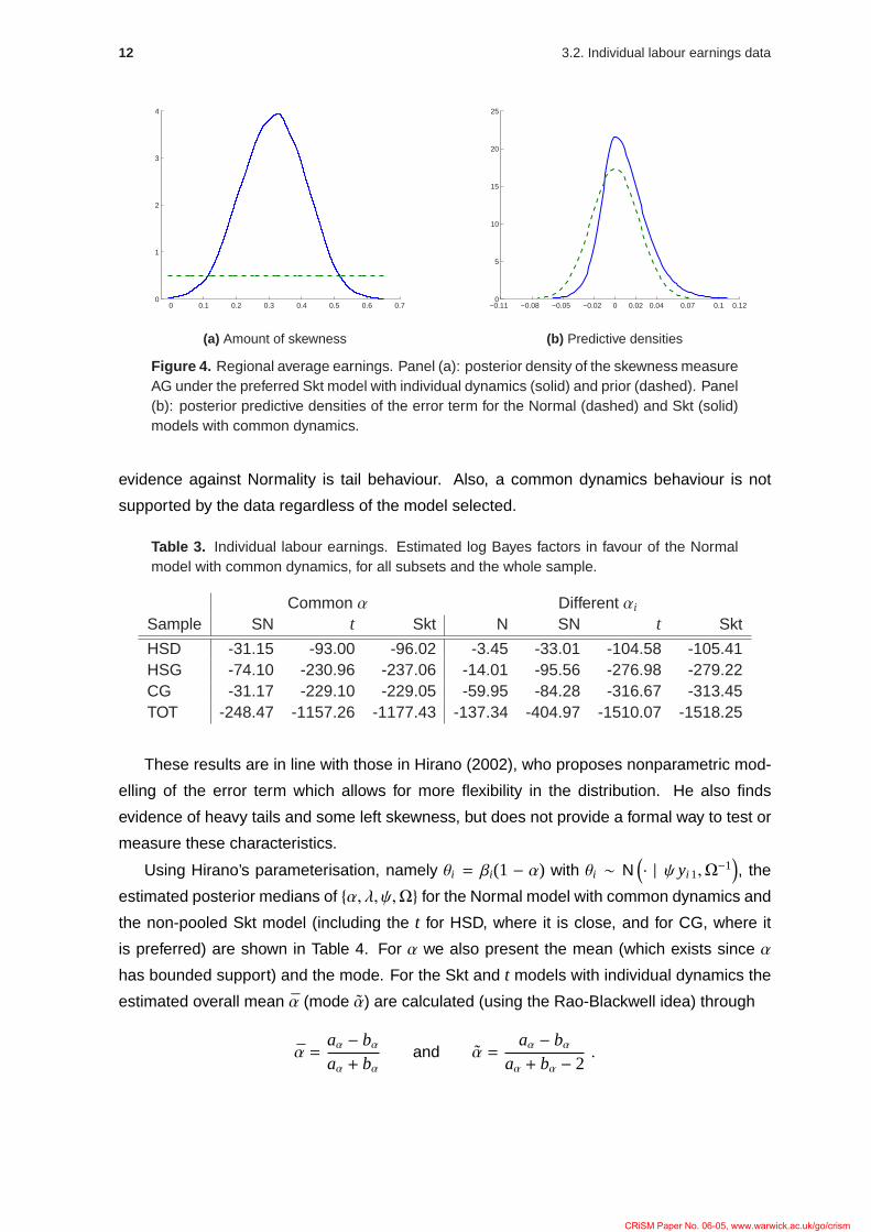
interpretable measure of skewness is AG, the posterior distribution of which is plotted in

Figure 4 (a), clearly indicating the overwhelming evidence in favour of right skewness. The

usual assumption of Normality (as used by Liu and Tiao, 1980 and Nandram and Petruccelli,

1997) is decisively rejected by the data (with BF=1.0× 105 for the pooled case and BF=1.4×106 for the unpooled case).

Of special interest is the behaviour of predictive distributions. Figure 4 (b) depicts the

posterior predictive distributions of the error term for the Normal and Skt models. The un-

equal distribution of the mass at either side of the mode is apparent for the Skt model; also,

the Normal model must adopt a much larger dispersion than the Skt in order to accommodate

the observations in the tails.

3.2 Individual labour earnings data

The data is drawn from the Panel Study of Income Dynamics (PSID) and records annual

labour earnings for males who were heads of households between the ages of 24 and 33,

during the period from 1967 to 1991. The data is filtered as described in Hirano (2002)4,

who constructs three subsets from the resulting 10 years of observations for 516 individuals,

according to their education: high school dropouts (HSD, m = 37), high school graduates

(HSG, m = 100) and college graduates (CG, m = 122). The full sample with m = 516will be

denoted by TOT.

As illustrated in Table 3 the data overwhelmingly favour the heavy-tailed models in both

scenarios. In contrast with the previous example, the feature that provides the strongest

p)/2 and (1 + p)/2 percentiles.4The log of the earnings is regressed on a constant, an indicator for race, indicators for different education

levels and calendar year. The residuals of the least-squares regression are then kept as the “raw data”.


12 3.2. Individual labour earnings data

0 0.1 0.2 0.3 0.4 0.5 0.6 0.70

1

2

3

4

(a) Amount of skewness

−0.11 −0.08 −0.05 −0.02 0 0.02 0.04 0.07 0.1 0.120

5

10

15

20

25

(b) Predictive densities

Figure 4. Regional average earnings. Panel (a): posterior density of the skewness measureAG under the preferred Skt model with individual dynamics (solid) and prior (dashed). Panel(b): posterior predictive densities of the error term for the Normal (dashed) and Skt (solid)models with common dynamics.

evidence against Normality is tail behaviour. Also, a common dynamics behaviour is not

supported by the data regardless of the model selected.

Table 3. Individual labour earnings. Estimated log Bayes factors in favour of the Normalmodel with common dynamics, for all subsets and the whole sample.


Sample SN t Skt N SN t Skt

HSD -31.15 -93.00 -96.02 -3.45 -33.01 -104.58 -105.41HSG -74.10 -230.96 -237.06 -14.01 -95.56 -276.98 -279.22CG -31.17 -229.10 -229.05 -59.95 -84.28 -316.67 -313.45TOT -248.47 -1157.26 -1177.43 -137.34 -404.97 -1510.07 -1518.25

These results are in line with those in Hirano (2002), who proposes nonparametric mod-

elling of the error term which allows for more flexibility in the distribution. He also finds

evidence of heavy tails and some left skewness, but does not provide a formal way to test or

measure these characteristics.

Using Hirano’s parameterisation, namely θi = βi(1 − α) with θi ∼ N(· | ψ yi 1,Ω

−1), the

estimated posterior medians of α, λ, ψ,Ω for the Normal model with common dynamics and

the non-pooled Skt model (including the t for HSD, where it is close, and for CG, where it

is preferred) are shown in Table 4. For α we also present the mean (which exists since α

has bounded support) and the mode. For the Skt and t models with individual dynamics the

estimated overall mean α (mode α) are calculated (using the Rao-Blackwell idea) through

α =aα − bαaα + bα

and α =aα − bα

aα + bα − 2.


3.2. Individual labour earnings data 13

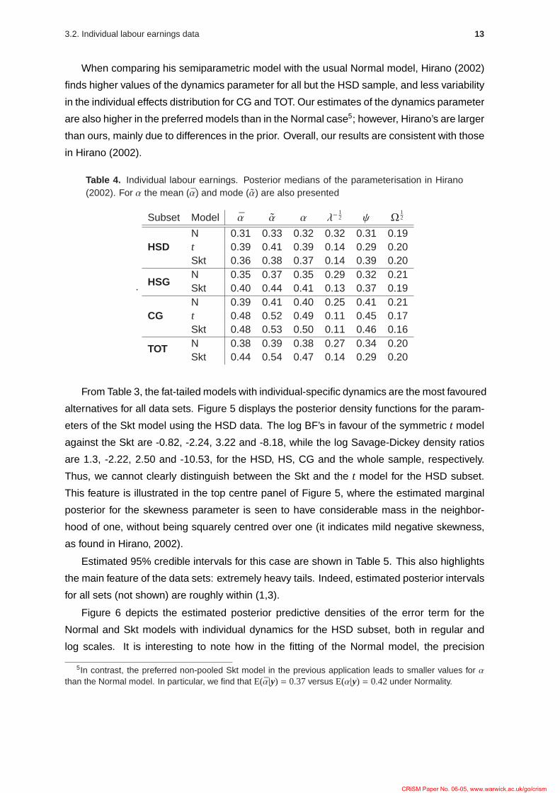
When comparing his semiparametric model with the usual Normal model, Hirano (2002)

finds higher values of the dynamics parameter for all but the HSD sample, and less variability

in the individual effects distribution for CG and TOT. Our estimates of the dynamics parameter

are also higher in the preferred models than in the Normal case5; however, Hirano’s are larger

than ours, mainly due to differences in the prior. Overall, our results are consistent with those

in Hirano (2002).

Table 4. Individual labour earnings. Posterior medians of the parameterisation in Hirano(2002). For α the mean (α) and mode (α) are also presented

.

Subset Model α α α λ−12 ψ Ω

12

N 0.31 0.33 0.32 0.32 0.31 0.19HSD t 0.39 0.41 0.39 0.14 0.29 0.20

Skt 0.36 0.38 0.37 0.14 0.39 0.20N 0.35 0.37 0.35 0.29 0.32 0.21

HSGSkt 0.40 0.44 0.41 0.13 0.37 0.19N 0.39 0.41 0.40 0.25 0.41 0.21

CG t 0.48 0.52 0.49 0.11 0.45 0.17Skt 0.48 0.53 0.50 0.11 0.46 0.16N 0.38 0.39 0.38 0.27 0.34 0.20TOTSkt 0.44 0.54 0.47 0.14 0.29 0.20

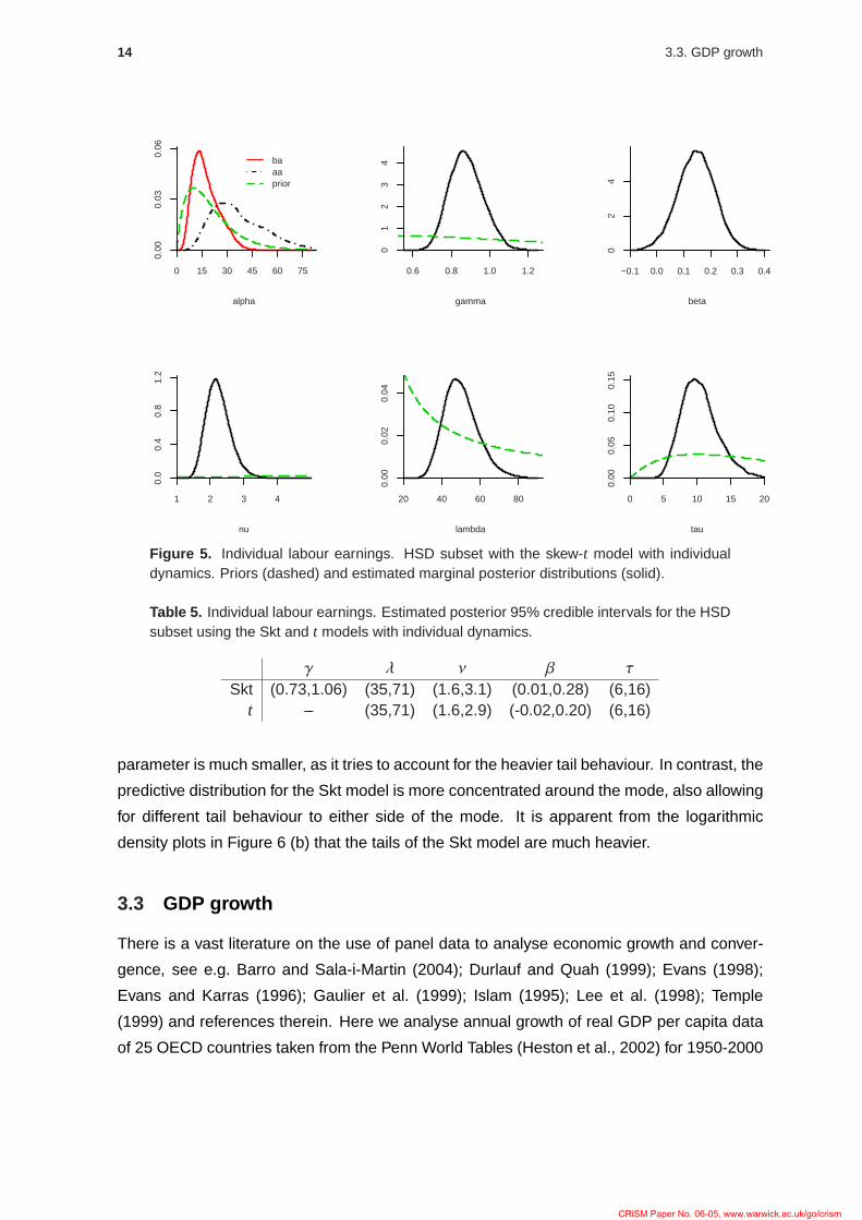
From Table 3, the fat-tailed models with individual-specific dynamics are the most favoured

alternatives for all data sets. Figure 5 displays the posterior density functions for the param-

eters of the Skt model using the HSD data. The log BF’s in favour of the symmetric t model

against the Skt are -0.82, -2.24, 3.22 and -8.18, while the log Savage-Dickey density ratios

are 1.3, -2.22, 2.50 and -10.53, for the HSD, HS, CG and the whole sample, respectively.

Thus, we cannot clearly distinguish between the Skt and the t model for the HSD subset.

This feature is illustrated in the top centre panel of Figure 5, where the estimated marginal

posterior for the skewness parameter is seen to have considerable mass in the neighbor-

hood of one, without being squarely centred over one (it indicates mild negative skewness,

as found in Hirano, 2002).

Estimated 95% credible intervals for this case are shown in Table 5. This also highlights

the main feature of the data sets: extremely heavy tails. Indeed, estimated posterior intervals

for all sets (not shown) are roughly within (1,3).

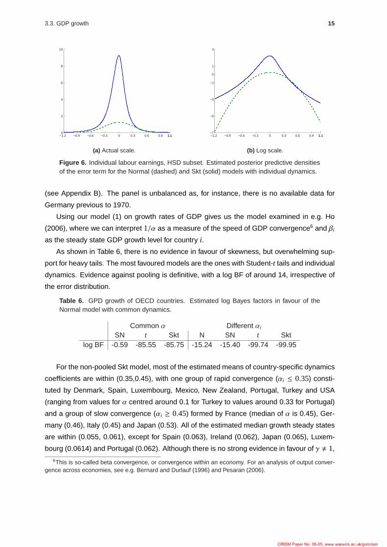
Figure 6 depicts the estimated posterior predictive densities of the error term for the

Normal and Skt models with individual dynamics for the HSD subset, both in regular and

log scales. It is interesting to note how in the fitting of the Normal model, the precision

5In contrast, the preferred non-pooled Skt model in the previous application leads to smaller values for αthan the Normal model. In particular, we find that E(α|y) = 0.37 versus E(α|y) = 0.42 under Normality.


14 3.3. GDP growth

alpha

baaaprior

0 15 30 45 60 75

0.00

0.03

0.06

gamma

0.6 0.8 1.0 1.2

01

23

4

beta

−0.1 0.0 0.1 0.2 0.3 0.4

02

4

nu

1 2 3 4

0.0

0.4

0.8

1.2

lambda

20 40 60 80

0.00

0.02

0.04

tau

0 5 10 15 20

0.00

0.05

0.10

0.15

Figure 5. Individual labour earnings. HSD subset with the skew-t model with individualdynamics. Priors (dashed) and estimated marginal posterior distributions (solid).

Table 5. Individual labour earnings. Estimated posterior 95% credible intervals for the HSDsubset using the Skt and t models with individual dynamics.

γ λ ν β τ

Skt (0.73,1.06) (35,71) (1.6,3.1) (0.01,0.28) (6,16)t – (35,71) (1.6,2.9) (-0.02,0.20) (6,16)

parameter is much smaller, as it tries to account for the heavier tail behaviour. In contrast, the

predictive distribution for the Skt model is more concentrated around the mode, also allowing

for different tail behaviour to either side of the mode. It is apparent from the logarithmic

density plots in Figure 6 (b) that the tails of the Skt model are much heavier.

3.3 GDP growth

There is a vast literature on the use of panel data to analyse economic growth and conver-

gence, see e.g. Barro and Sala-i-Martin (2004); Durlauf and Quah (1999); Evans (1998);

Evans and Karras (1996); Gaulier et al. (1999); Islam (1995); Lee et al. (1998); Temple

(1999) and references therein. Here we analyse annual growth of real GDP per capita data

of 25 OECD countries taken from the Penn World Tables (Heston et al., 2002) for 1950-2000


3.3. GDP growth 15

−1.2 −0.9 −0.6 −0.3 0 0.3 0.6 0.9 1.11.10

2

4

6

8

10

(a) Actual scale.

−1.2 −0.9 −0.6 −0.3 0 0.3 0.6 0.9 1.11.1−7

−5

−3

−1

0

1

3

(b) Log scale.

Figure 6. Individual labour earnings, HSD subset. Estimated posterior predictive densitiesof the error term for the Normal (dashed) and Skt (solid) models with individual dynamics.

(see Appendix B). The panel is unbalanced as, for instance, there is no available data for

Germany previous to 1970.

Using our model (1) on growth rates of GDP gives us the model examined in e.g. Ho

(2006), where we can interpret 1/α as a measure of the speed of GDP convergence6 and βi

as the steady state GDP growth level for country i.

As shown in Table 6, there is no evidence in favour of skewness, but overwhelming sup-

port for heavy tails. The most favoured models are the ones with Student-t tails and individual

dynamics. Evidence against pooling is definitive, with a log BF of around 14, irrespective of

the error distribution.

Table 6. GPD growth of OECD countries. Estimated log Bayes factors in favour of theNormal model with common dynamics.


SN t Skt N SN t Sktlog BF -0.59 -85.55 -85.75 -15.24 -15.40 -99.74 -99.95

For the non-pooled Skt model, most of the estimated means of country-specific dynamics

coefficients are within (0.35,0.45), with one group of rapid convergence (αi ≤ 0.35) consti-

tuted by Denmark, Spain, Luxembourg, Mexico, New Zealand, Portugal, Turkey and USA

(ranging from values for α centred around 0.1 for Turkey to values around 0.33 for Portugal)

and a group of slow convergence (αi ≥ 0.45) formed by France (median of α is 0.45), Ger-

many (0.46), Italy (0.45) and Japan (0.53). All of the estimated median growth steady states

are within (0.055, 0.061), except for Spain (0.063), Ireland (0.062), Japan (0.065), Luxem-

bourg (0.0614) and Portugal (0.062). Although there is no strong evidence in favour of γ , 1,

6This is so-called beta convergence, or convergence within an economy. For an analysis of output conver-gence across economies, see e.g. Bernard and Durlauf (1996) and Pesaran (2006).


16 3.3. GDP growth

around 89% of the posterior mass of γ (AG) is to the right of 1 (0), which could be caused by

the model accounting for these few countries with growth rates above the average. Fat tails

account for the greatest evidence against Normality, with (3.0, 4.7) a 95% posterior credible

interval for ν.

Based on the results above, we decided to break the data up into four disjoint subsets,

as listed in Appendix B: core-EU (CEU), with 13 countries; rest-EU (REU), with m = 6; North

America (NA), m = 3; and East Asia (EA), m = 3, and to estimate a separate model for each

group. The resulting BF’s support pooling within all subsets, and only suggest weak evidence

against pooling for the REU and EA subsets when using either t models (log BF = -1.7 and

-1.4, respectively). As shown in Table 7, there is, again, no real evidence of skewness

in any subset, the salient feature against Normality being fat tails (Med[νCEU | y] = 3.8,

Med[νREU | y] = 4.4, Med[νEA | y] = 13.2). This is true for all but the NA subset, for which

the pooled Normal model is not definitively rejected (Med[νNA | y] = 20.2), with a log BF in

favour of the Normal pooled model against the Skt of around -1.1. The posterior credible

intervals for α of the two European subsets do not overlap, creating two well separated clubs

of slow and rapid growth dynamics, which ties in the concept of convergence clubs in Quah

(1997) and the evidence in favour of different regimes in Durlauf and Johnson (1995) and

Canova (2004). This is not the case for the other two subsets, which might be merged in a

subsequent analysis. An alternative to this grouping into subsets is to use a double-threshold

model as in Hansen (1999) and Ho (2006), which allows for different speeds of convergence

depending on the income levels.

Table 7. GPD growth of OECD countries. Estimated 95% credible intervals for the param-eters using the pooled Normal and Skt models for the four subsets and the whole sample(figures for λ are in thousands and in tens of thousands for τ).

α γ ν β τ (×104) λ (×103)N (0.26, 0.40) – – (0.059, 0.067) (1.09, 6.12) (0.90, 1.12)

CEUSkt (0.36, 0.50) (0.97, 1.19) (3 , 5) (0.050, 0.064) (1.14, 6.23) (1.65, 2.49)

N (-0.07,0.14) – – (0.064, 0.076) (1.12, 11.3) (0.36, 0.50)REU

Skt (0.03, 0.24) (0.88, 1.19) (3, 8) (0.058, 0.080) (4.11, 61.4) (0.61, 1.08)

N (0.20, 0.48) – – (0.049, 0.067) (28, 621) (0.56, 0.88)NA

Skt (0.20, 0.48) (0.74, 1.10) (6, 60) (0.050, 0.084) (85, 1926) (0.63, 1.14)

N (0.21, 0.50) – – (0.039, 0.085) (0.09,1.32) (0.64, 1.01)EA

Skt (0.27, 0.57) (0.85, 1.34) (5, 44) (0.030, 0.080) (0.02, 3.97) (0.75, 1.41)

N (0.19, 0.29) – – (0.059, 0.069) (0.49, 1.63) (0.64, 0.75)OECD

Skt (0.29, 0.40) (0.97,1.13) (3, 5) (0.054, 0.068) (0.05, 1.69) (1.20, 1.60)


4. Conclusions 17

In the case of the European countries, estimates for the dynamics parameter are clearly

lower under Normality than when allowing for fat tails and skewness, thus erroneously sug-

gesting a more rapid convergence in the former case. It is also apparent how the estimated

observation precision, λ, must be much lower in the Normal case in order for the model to

accommodate the observations in the tails. Remarkably, the estimates of the hyperparam-

eter β are fairly similar, indicating that at least the mean of the distribution of the individual

effects is not much affected by the choice of error distribution. In the case of CEU the same

holds for the entire individual effects distribution.

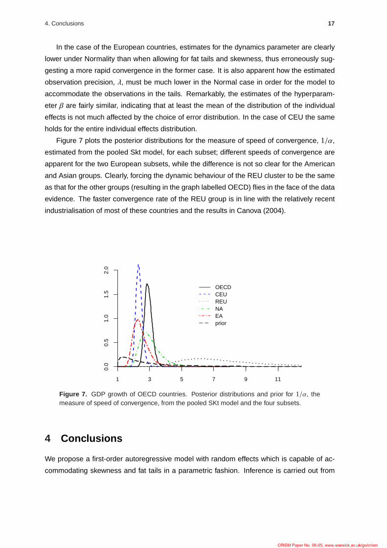
Figure 7 plots the posterior distributions for the measure of speed of convergence, 1/α,

estimated from the pooled Skt model, for each subset; different speeds of convergence are

apparent for the two European subsets, while the difference is not so clear for the American

and Asian groups. Clearly, forcing the dynamic behaviour of the REU cluster to be the same

as that for the other groups (resulting in the graph labelled OECD) flies in the face of the data

evidence. The faster convergence rate of the REU group is in line with the relatively recent

industrialisation of most of these countries and the results in Canova (2004).

1 3 5 7 9 11

0.0

0.5

1.0

1.5

2.0

OECDCEUREUNAEAprior

Figure 7. GDP growth of OECD countries. Posterior distributions and prior for 1/α, themeasure of speed of convergence, from the pooled SKt model and the four subsets.

4 Conclusions

We propose a first-order autoregressive model with random effects which is capable of ac-

commodating skewness and fat tails in a parametric fashion. Inference is carried out from


18 4. Conclusions

a Bayesian perspective and a sensible prior structure is proposed that does not incorporate

strong prior beliefs and which allows for comparisons across models. Further, an alternative

model, which allows the dynamics to change over individuals, is considered. Estimation is

done numerically through MCMC techniques.

The methodology is illustrated with three real data sets. The application to regional av-

erage earnings data strongly favours skewed models with moderately fat tails, whereas the

evidence against Normality for the other data sets mostly centers around fat tails. However,

in some cases fat tails may partially account for skewness and vice versa, and therefore

it is important to treat both quantities as unknown and estimate them simultaneously. The

applications to individual earnings data and to the growth of countries provide conclusive

evidence against the assumption of common dynamics. The latter data, however, allow for

pooling once the individual countries are clustered into four, more homogeneous, groups.

Interestingly, for those cases where fat tails are strongly supported, the usual Normal model

leads to substantially smaller values for the dynamics parameter. This is of particular interest

for the application to economic growth, where this parameter is directly linked to the speed

of GDP convergence.

Several extensions to the model are possible. In some cases, the interest of the re-

searcher lies primarily in the effect of certain covariates. For instance, it may be of special

interest to investigate the degree of influence of race, schooling, etc. on the income dynamics

of individuals; or the effect of human capital, investment, etc. on economic growth. In that

case, it is natural to include a set of covariates grouped in a ti × p matrix Xi , such that

yi t = βi (1− α) + α yi t−1 + xit δ + λ−

12εi t ,

where δ = (δ1, . . . , δp)′ are the additional parameters, with prior π(δ), and xit is the t-th

row of Xi . This can be accommodated straightforwardly within the procedure described in

the paper, just by adding an extra step in the sampler for the new parameters. Such an

extension would be natural for all the applications treated in the paper. Recall that Hirano’s

data (also used in Subsection 3.2) are in fact residuals from a least-squares regression on a

number of covariates, and including these covariates in the model would be preferable, both

from a methodological perspective and an empirical one. Inference on δ might well depend

quite crucially on the distributional assumptions on the error term.

Another extension that is fairly easy to implement is to include in the model a distribution

for yi 0, the initial value, rather than conditioning on a fixed value. This could be particularly

important in cases where the time dimension of the panels are relatively short (such as the

Hirano data).

We feel that testing for heterogeneity from a Bayesian perspective offers a mayor ad-


19

vantage. Bayes factors are well-defined for any number of individuals m and repeated mea-

sures through time Ti , as long as the posteriors and priors on model-specific parameters are

proper. In contrast, most of the alternative frequentist tests are based on semi-asymptotic

results (see e.g. Pesaran et al., 1995, and references therein) whose conditions are often

not met in practice or are difficult to check.

With our methodology we can easily test whether to pool the dynamics across the whole

panel. Of course, trying to find clusters of units exhibiting similar dynamic behaviour can

be of paramount interest in some applications, such as growth economics (Arbia and Piras,

2005; Canova, 2004; Quah, 1997). In this paper, we have used the model with individual dy-

namics to suggest a useful clustering of the individuals into relatively homogeneous groups.

Whereas that often works reasonably well in practice, this approach can be deemed some-

what ad-hoc.7 Thus, we also intend to make the clustering mechanism part of the model and

allow for a free selection of the number and composition of clusters within the model, follow-

ing previous approaches in Canova (2004) and Frühwirth-Schnatter and Kaufmann (2004).

Using a hierarchical framework, this would be a natural extension of the model and algorithm

and is the topic of ongoing research.

Acknowledgements

We gratefully acknowledge comments from participants of the 13th International Conference

on Panel Data, Cambridge. This research was supported by the UK research council EPSRC

under grant number GR/T17908/01.

Appendix A Proofs

A.1 Proof of Theorem 1

The proof is done in two steps. First, we will prove that the posterior is proper for γ > 0 if and

only if (iff) it is proper for γ = 1. Then, we will prove propriety of the posterior for the simpler

cases of the Normal and Student distributions.

For step one, we use Theorem 1 of Fernández and Steel (1998) which states that the

posterior of the skew model is proper iff it is proper when γ = 1. So we write

I =

m∏

i=1

Ti∏

t=1

f (yi t | α, β, γ, τ, λ, ν) dPα dPβ dPγ dPτ dPλ dPν .

7Although it perhaps has the advantage that it is not totally mechanical and considerations beyond statisticalfit can be taken into account, as was done in our application in Subsection 3.3.


20

Clearly f (s) = f (|s|) is decreasing in |s|, so the same upper and lower bounds for the sam-

pling density as in Fernández and Steel (1998) hold, and using gi(θ) = βi (1 − α) + α yi t−1

these bounds are given by

2 λ12

γ + γ−1f

λ12 |yi t − gi(θ)|

h(γ)

,with

h(γ) =

max

γ, γ−1

for the upper bound

minγ, γ−1

for the lower bound.

Therefore, I < ∞ iff I < ∞ under γ = 1.

In step two we write the model as y = X θ + ε, with

y =

y1 1...

y1T1

y2 1...

ym Tm

, X =

1T1 0T1,m−1 y1

0T2,1 1T2 0T2,m−2 y2...

. . . . . ....

0Tm,m−1 1Tm ym

and θ =

β1 (1− α)

β2 (1− α)...

βm (1− α)

α

where yi =yi0, . . . , yiTi−1

, 1k is a k-dimensional vector of ones and 0A,B is an A× B matrix

of zeros. So, y ∈ RT , X is a full column rank matrix of size T × (m+ 1) and θ ∈ Rm+1, with

T =∑m

i=1 Ti the total number of observations.

We now use Theorem 3 of Fernández et al. (1997), which states that the posterior distri-

bution exists if π(θ1, . . . , θm) is bounded, π(α) is proper and T is strictly greater than the rank

of X.

Normal case After integrating out λ we have that the posterior is proper iff the integral

I =

[(y− X θ

)′ (y− X θ

)]−T /2π(θ) dθ

is finite.

From the prior specification, we have for i = 1, . . . ,m

θi | α, β, τ ∼ N(θi | β (1− α), τ/(1− α)2

)

and so

π(θi) =

N

(θi | β (1− α), τ/(1− α)2

)π(β, τ)π(α) dβ dτ dα


21

with π(β, τ) = cτaτ−1 exp[−bττ]. Given that N (· | µ, ϕ) < ϕ1/2, we have that

π(θi) ≤ c

τ12

(1− α)τaτ−1 exp[−bττ] π(α) dτ dα

≤ c′

(1 + α)aα−1(1− α)bα−2 dα,

which is bounded if bα > 1, as imposed in (11).

Therefore, given that the rank of X is m+ 1, I < ∞ if T > m+ 1.

Student case Let us consider the t distribution as a scale mixture of Normals as in Fernán-

dez and Steel (2000). So, after integrating out λ, the posterior is proper if the integral

I =

[(y− X θ

)′Ω

(y− X θ

)]−T /2π(θ)π(Ω | ν)π(ν) dθ dΩ dν

is finite, where Ω = diagωi t, t = 1 . . . ,Ti , i = 1, . . . ,m is a diagonal matrix with the

T (augmented) mixing parameters and π(ωi t | ν) = Ga (ωi t | ν/2, ν/2), i.i.d.

Now we use the same argument as in the Normal case to prove that π(θ1, . . . , θm) is

bounded, provided that bα > 1. Further, Theorem 4(ii) of Fernández and Steel (2000)

provides an upper bound for the integral above if T > m+ 1.

A.2 Proof of Theorem 2

This proof is almost identical to that of Theorem 1, except that the parameterisation in step

two now becomes

X =

1T1 0T1,m−1 y1 0T1,m−1

0T2,1 1T2 0T2,m−1 y2 0T2,m−2...

. . . . . . . . .. . .

...

0Tm,m−1 1Tm 0Tm,m−1 ym

and θ =

β1 (1− α1)

β2 (1− α2)...

βm (1− αm)

α1

α2...

αm

so that X is now a full column rank matrix of size T × 2m and θ ∈ R2m. Following the same

reasoning as in Theorem 1, a sufficient condition for posterior existence is T > 2m.


22

Appendix B List of OECD countries

Core-EU Rest-EU North America East Asia

Austria Great Britain Spain Canada Australia

Belgium Germany Greece Mexico Japan

Switzerland Iceland Ireland USA New Zealand

Denmark Italy Luxembourg

Finland Netherlands Portugal

France Norway Turkey

Sweden

References

Arbia, G. and Piras, G. (2005). Convergence in per-capita GDP across European regions

using panel data models extended to spatial autocorrelation effects, Working Paper 51,

Istituto di Studi e Analisi Economica, Roma.

Arellano, M. (2003). Panel Data Econometrics, Oxford: Oxford University Press.

Arnold, B. C. and Beaver, R. J. (2002). Skewed multivariate models related to hidden trunca-

tion and/or selective reporting, Test, 11, 7–54.

Arnold, B. C. and Groeneveld, R. A. (1995). Measuring skewness with respect to the mode,

The American Statistician, 49, 34–38.

Azzalini, A. (1985). A class of distributions which include the normal ones, Scandinavian

Journal of Statistics, 12, 171–178.

Azzalini, A. and Capitanio, A. (2003). Distributions generated by perturbations of symmetry

with emphasis on a multivariate skew t-distribution, Journal of the Royal Statistical Society,

B, 65, 367–389.

Baltagi, B. (2001). Econometric Analysis of Panel Data, Chichester: Wiley, second ed.

Barro, R. J. and Sala-i-Martin, X. (2004). Economic Growth, Cambridge: MIT Press, second

ed.

Bernard, A. B. and Durlauf, S. N. (1996). Interpreting tests of the convergence hypothesis,

Journal of Econometrics, 71, 161–173.


23

Canova, F. (2004). Testing for convergence clubs in income per capita: A predictive density

approach, International Economic Review, 45, 49–77.

Chib, S. and Greenberg, E. (1994). Bayes inference in regression models with ARMA(p,q)

errors, Journal of Econometrics, 64, 183–206.

Durlauf, S.N. and Johnson, P.A. (1995). Multiple regimes and cross-country growth be-

haviour, Journal of Applied Econometrics, 10, 365–384.

Durlauf, S.N. and Quah, D.T. (1999). The new empirics of economic growth, Handbook of

Macroeconomics Vol.1 (J.B. Taylor and M. Woodford, eds.), Amsterdam: Elsevier, pp. 235–

308.

Evans, P. (1998). Using panel data to evaluate growth theories, International Economic Re-

view, 39, 295–306.

Evans, P. and Karras, G. (1996). Do economies converge? Evidence from a panel of US

states, The review of Economics and Statistics, 78, 348–388.

Fernández, C., Osiewalski, J. and Steel, M. F. J. (1997). On the use of panel data in stochas-

tic frontier models with improper priors, Journal of Econometrics, 79, 169–193.

Fernández, C. and Steel, M. F. J. (1998). On Bayesian modeling of fat tails and skewness,

Journal of the American Statistical Association, 93, 359–371.

Fernández, C. and Steel, M. F. J. (2000). Bayesian regression analysis with scale mixtures

of normals, Econometric Theory, 16, 80–101.

Frühwirth-Schnatter, S. and Kaufmann, S. (2004). Model-based clustering of multiple time

series, mimeo, Johannes Kepler Universität Linz.

Gaulier, G., Hurlin, C. and Jean-Pierre, P. (1999). Testing convergence: A panel data ap-

proach, Annales D’économie et de Statistique, 55-56, 411–427.

Gelman, A. (2006). Prior distributions for variance parameters in hierarchical models,

Bayesian Analysis, 1, 515–534.

Genton, M. G. (2004). Skew-Elliptical Distributions and Their Applications: A Journey Beyond

Normality, Boca Raton: Chapman & Hall.

Hansen, B.E. (1999). Threshold effects in non-dynamic panels: estimation, testing and infer-

ence, Journal of Econometrics, 93, 334–368.


24

Heston, A., Summers, R. and Aten, B. (2002). Penn world table version 6.1,

http://pwt.econ.upenn.edu/php_site/pwt_index.php. Center for International Com-

parisons at the University of Pennsylvania (CICUP).

Hill, B. M. (1965). Inference about variance components in the one-way model, Journal of

the American Statistical Association, 60, 806–825.

Hirano, K. (2002). Semiparametric Bayesian inference in autoregressive panel data models,

Econometrica, 70, 781–799.

Ho, T. (2006). Income thresholds and growth convergence: A panel data approach, The

Manchester School, 74, 170–189.

Hsiao, C. and Pesaran, M. H. (2004). Random coefficient panel data models, IEPR Working

Paper 04.2, University of Southern California.

Islam, N. (1995). Growth empirics: a panel data approach, Quarterly Journal of Economics,

110, 1128–1170.

Jones, M. C. and Faddy, M. J. (2003). A skew extension of the t-distribution, with applications,

Journal of the Royal Statistical Society, B, 65, 159–174.

Lee, M., Longmire, R., Mátyás, L. and Harris, M. (1998). Growth convergence: some panel

data evidence, Applied Economics, 30, 907–912.

Liu, M. C. and Tiao, G. C. (1980). Random coefficient first-order autoregressive models,

Journal of Econometrics, 13, 305–325.

Mátyás, L. and Sevestre, P. (1995). The Econometrics of Panel Data. A handbook of the

theory with applications, The Netherlands: Kluwer, second ed.

Nandram, B. and Petruccelli, J. D. (1997). A Bayesian analysis of autoregressive time series

panel data, Journal of Business and Economic Statistics, 15, 328–334.

Newton, M. A. and Raftery, A. E. (1994). Approximate Bayesian inference with the weighted

likelihood bootstrap, Journal of the Royal Statistical Society, B, 56, 3–48.

Pesaran, M. H. (2006). A pair-wise approach to testing for output and growth convergence,

Journal of Econometrics, forthcoming.

Pesaran, M. H., Smith, R. and Im, K. S. (1995). Dynamic linear models for heterogenous pan-

els, The Econometrics of Panel Data (L. Mátyás and P. Sevestre, eds.), The Netherlands:

Kluwer, pp. 145–195.


25

Quah, D. T. (1997). Empirics for growth and distribution: Stratification, polarization and con-

vergence clubs, Journal of Economic Growth, 2, 27–59.

Sáfadi, T. and Morettin, P. A. (2003). A Bayesian analysis of autoregressive models with

random Normal coefficients, Journal of Statistical Computation and Simulation, 8, 563–

573.

Spiegelhalter, D. J., Abrams, K. R. and Myles, J. P. (2004). Bayesian approaches to clinical

trials and health-care evaluation, Chichester: Wiley.

Sun, D., Tsutakawa, R. K. and He, Z. (2001). Property of posteriors with improper priors in

hierarchical linear mixed models, Statistica Sinica, 11, 77–95.

Temple, J. (1999). The new growth evidence, Journal of Economic Literature, 37, 112–156.

Verdinelli, I. and Wasserman, L. (1995). Computing Bayes factors using a generalization

of the Savage-Dickey density ratio, Journal of the American Statistical Association, 90,

614–618.

Wang, D. and Ghosh, S. K. (2002). Bayesian analysis of random coefficient autoregressive

models, Joint Statistical meeting proceedings.

Zellner, A. (1971). An introduction to Bayesian inference in Econometrics, New York: Wiley.


Documents

Non-gaussian dynamic bayesian modelling for panel data