Embed Size (px)
Citation preview
arX
iv:1
311.
1521
v2 [
hep-
th]
22
Nov
201
3
(Non)–Integrability of Geodesics in D–brane Backgrounds
Yuri Chervonyi and Oleg Lunin
Department of Physics,University at Albany (SUNY),
Albany, NY 12222, USA
Abstract
Motivated by the search for new backgrounds with integrable string theories, we classifythe D–brane geometries leading to integrable geodesics. Our analysis demonstrates that theHamilton–Jacobi equation for massless geodesics can only separate in elliptic or sphericalcoordinates, and all known integrable backgrounds are covered by this separation. In par-ticular, we identify the standard parameterization of AdSp×Sq with elliptic coordinates ona flat base. We also find new geometries admitting separation of the Hamilton–Jacobi equa-tion in the elliptic coordinates. Since separability of this equation is a necessary conditionfor integrability of strings, our analysis gives severe restrictions on the potential candidatesfor integrable string theories.
[email protected], [email protected]
1
Contents
1 Introduction and summary 3
2 Examples: spherical and elliptic coordinates 6
3 Geodesics in D–brane backgrounds 83.1 Reduction to two dimensions . . . . . . . . . . . . . . . . . . . . . . . . . . . . . . . . . . 83.2 Separation of variables and elliptic coordinates . . . . . . . . . . . . . . . . . . . . . . . . 123.3 Properties of the brane sources . . . . . . . . . . . . . . . . . . . . . . . . . . . . . . . . . 17
4 Beyond geodesics: wave equation, Killing tensors, and strings 214.1 Separability of the wave equation . . . . . . . . . . . . . . . . . . . . . . . . . . . . . . . . 214.2 Killing tensor . . . . . . . . . . . . . . . . . . . . . . . . . . . . . . . . . . . . . . . . . . . 234.3 Non–integrability of strings . . . . . . . . . . . . . . . . . . . . . . . . . . . . . . . . . . . 24
5 Geodesics in static Dp–D(p+ 4) backgrounds 27
6 Geodesics in D1–D5 microstates 30
7 Geodesics in bubbling geometries. 35
8 Elliptic coordinates and standard parameterization of AdSp×Sq 39
9 Discussion 44
A Examples of separable Hamilton–Jacobi equations 45A.1 Motion on a sphere . . . . . . . . . . . . . . . . . . . . . . . . . . . . . . . . . . . . . . . . 45A.2 Two–center potential and elliptic coordinates . . . . . . . . . . . . . . . . . . . . . . . . . 46
B Ellipsoidal coordinates 48B.1 Ellipsoidal coordinates for k = 3 . . . . . . . . . . . . . . . . . . . . . . . . . . . . . . . . 48B.2 Ellipsoidal coordinates for k > 3 . . . . . . . . . . . . . . . . . . . . . . . . . . . . . . . . 54
C Equation for geodesics in D–brane backgrounds 56C.1 Particles without angular momentum . . . . . . . . . . . . . . . . . . . . . . . . . . . . . . 57C.2 General case . . . . . . . . . . . . . . . . . . . . . . . . . . . . . . . . . . . . . . . . . . . . 61
D Equations for Killing tensors 62D.1 Killing tensors for the metric produced by D–branes . . . . . . . . . . . . . . . . . . . . . 62D.2 Review of Killing tensors for flat space . . . . . . . . . . . . . . . . . . . . . . . . . . . . . 65
E Non–integrability of strings on D–brane backgrounds 67E.1 Review of analytical non–integrability . . . . . . . . . . . . . . . . . . . . . . . . . . . . . 67E.2 Application to strings in Dp–brane backgrounds . . . . . . . . . . . . . . . . . . . . . . . 69E.3 Application to geometries with integrable geodesics . . . . . . . . . . . . . . . . . . . . . . 71
F Geodesics in bubbling geometries. 72F.1 Geometries with AdS5×S5 asymptotics . . . . . . . . . . . . . . . . . . . . . . . . . . . . . 72F.2 Geometries with pp–wave asymptotics . . . . . . . . . . . . . . . . . . . . . . . . . . . . . 75F.3 Geometries dual to SYM on a circle . . . . . . . . . . . . . . . . . . . . . . . . . . . . . . 78
2
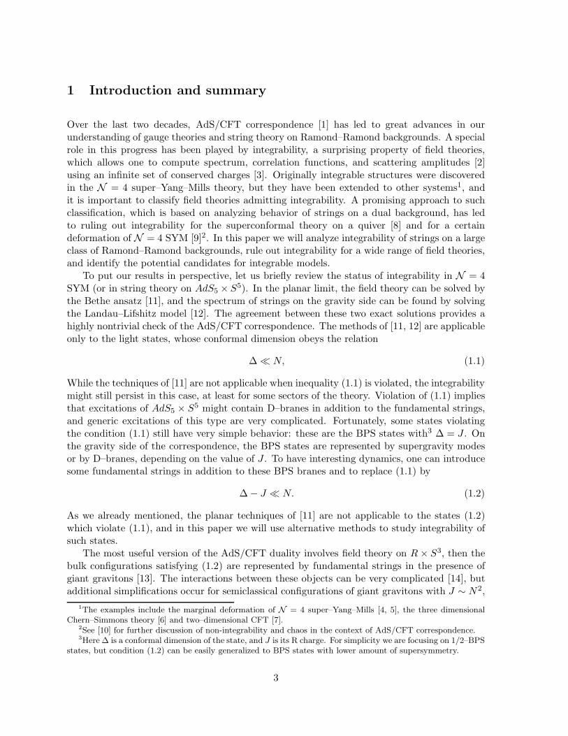
1 Introduction and summary
Over the last two decades, AdS/CFT correspondence [1] has led to great advances in ourunderstanding of gauge theories and string theory on Ramond–Ramond backgrounds. A specialrole in this progress has been played by integrability, a surprising property of field theories,which allows one to compute spectrum, correlation functions, and scattering amplitudes [2]using an infinite set of conserved charges [3]. Originally integrable structures were discoveredin the N = 4 super–Yang–Mills theory, but they have been extended to other systems1, andit is important to classify field theories admitting integrability. A promising approach to suchclassification, which is based on analyzing behavior of strings on a dual background, has ledto ruling out integrability for the superconformal theory on a quiver [8] and for a certaindeformation of N = 4 SYM [9]2. In this paper we will analyze integrability of strings on a largeclass of Ramond–Ramond backgrounds, rule out integrability for a wide range of field theories,and identify the potential candidates for integrable models.
To put our results in perspective, let us briefly review the status of integrability in N = 4SYM (or in string theory on AdS5 × S5). In the planar limit, the field theory can be solved bythe Bethe ansatz [11], and the spectrum of strings on the gravity side can be found by solvingthe Landau–Lifshitz model [12]. The agreement between these two exact solutions provides ahighly nontrivial check of the AdS/CFT correspondence. The methods of [11, 12] are applicableonly to the light states, whose conformal dimension obeys the relation
∆ ≪ N, (1.1)
While the techniques of [11] are not applicable when inequality (1.1) is violated, the integrabilitymight still persist in this case, at least for some sectors of the theory. Violation of (1.1) impliesthat excitations of AdS5 × S5 might contain D–branes in addition to the fundamental strings,and generic excitations of this type are very complicated. Fortunately, some states violatingthe condition (1.1) still have very simple behavior: these are the BPS states with3 ∆ = J . Onthe gravity side of the correspondence, the BPS states are represented by supergravity modesor by D–branes, depending on the value of J . To have interesting dynamics, one can introducesome fundamental strings in addition to these BPS branes and to replace (1.1) by
∆− J ≪ N. (1.2)
As we already mentioned, the planar techniques of [11] are not applicable to the states (1.2)which violate (1.1), and in this paper we will use alternative methods to study integrability ofsuch states.
The most useful version of the AdS/CFT duality involves field theory on R× S3, then thebulk configurations satisfying (1.2) are represented by fundamental strings in the presence ofgiant gravitons [13]. The interactions between these objects can be very complicated [14], butadditional simplifications occur for semiclassical configurations of giant gravitons with J ∼ N2,
1The examples include the marginal deformation of N = 4 super–Yang–Mills [4, 5], the three dimensionalChern–Simmons theory [6] and two–dimensional CFT [7].
2See [10] for further discussion of non-integrability and chaos in the context of AdS/CFT correspondence.3Here ∆ is a conformal dimension of the state, and J is its R charge. For simplicity we are focusing on 1/2–BPS
states, but condition (1.2) can be easily generalized to BPS states with lower amount of supersymmetry.
3
which can be viewed as classical geometries [15]. In this regime of parameters, integrability ofthe sector (1.2) reduces to integrability of strings on the bubbling geometries constructed in[15]. If the CFT is formulated on R3,1, the counterparts of the bubbling geometries are given bybrane configurations describing the Coulomb branch of N = 4 SYM [16]. In the latter case, onecan introduce an additional deformation which connects AdS5 × S5 asymptotics to flat spaceand see whether integrability persists for such configurations.
It turns out that the answer to the last question is no, and this result discovered in [9]was the main motivation for our investigation. As demonstrated in [9], addition of one to theharmonic function describing a single stack of D3 branes destroys integrability of the closedstrings on a new asymptotically-flat background. Since continuation to the flat asymptoticsdestroys the dual field theory, this procedure appears to be more drastic than a transition tothe Coulomb branch, which corresponds to a normalizable excitations, so the latter might havea chance to remain integrable. In this paper we focus on geometries dual to the Coulombbranch of N = 4 SYM (either on R3,1 or on R× S3) and on similar geometries involving otherD branes. A different class of theories, which involves putting D branes on singular manifolds,was explored in [8], where it was demonstrated that strings are not integrable on the conifold.From the point of view of field theory, this result pertains to the vacuum of N = 1 SYM witha quiver gauge group, which is complementary to our analysis of excited states in N = 4 SYM.
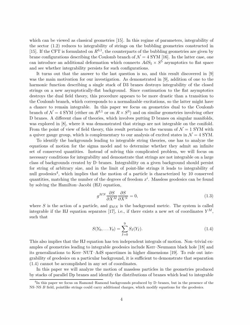
To identify the backgrounds leading to integrable string theories, one has to analyze theequations of motion for the sigma model and to determine whether they admit an infiniteset of conserved quantities. Instead of solving this complicated problem, we will focus onnecessary conditions for integrability and demonstrate that strings are not integrable on a largeclass of backgrounds created by D–branes. Integrability on a given background should persistfor string of arbitrary size, and in the limit of point-like strings it leads to integrability ofnull geodesics4, which implies that the motion of a particle is characterized by 10 conservedquantities, matching the number of the degrees of freedom xi. Massless geodesics can be foundby solving the Hamilton–Jacobi (HJ) equation,
gMN ∂S
∂XM
∂S
∂XN= 0, (1.3)
where S is the action of a particle, and gMN is the background metric. The system is calledintegrable if the HJ equation separates [17], i.e., if there exists a new set of coordinates YM ,such that
S(Y0, . . . Y9) =
9∑
I=0
SI(YI). (1.4)
This also implies that the HJ equation has ten independent integrals of motion. Non–trivial ex-amples of geometries leading to integrable geodesics include Kerr–Neumann black hole [18] andits generalizations to Kerr–NUT–AdS spacetimes in higher dimensions [19]. To rule out inte-grability of geodesics on a particular background, it is sufficient to demonstrate that separation(1.4) cannot be accomplished in any set of coordinates.
In this paper we will analyze the motion of massless particles in the geometries producedby stacks of parallel Dp branes and identify the distributions of branes which lead to integrable
4In this paper we focus on Ramond–Ramond backgrounds produced by D–branes, but in the presence of theNS–NS B field, pointlike strings could carry additional charges, which modify equations for the geodesics.
4
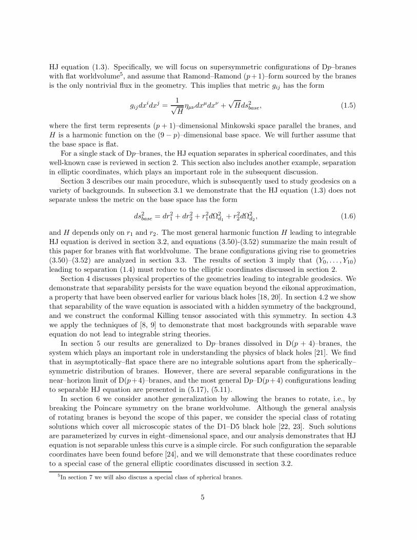
HJ equation (1.3). Specifically, we will focus on supersymmetric configurations of Dp–braneswith flat worldvolume5, and assume that Ramond–Ramond (p+1)–form sourced by the branesis the only nontrivial flux in the geometry. This implies that metric gij has the form
gijdxidxj =
1√Hηµνdx
µdxν +√Hds2base, (1.5)
where the first term represents (p + 1)–dimensional Minkowski space parallel the branes, andH is a harmonic function on the (9 − p)–dimensional base space. We will further assume thatthe base space is flat.
For a single stack of Dp–branes, the HJ equation separates in spherical coordinates, and thiswell-known case is reviewed in section 2. This section also includes another example, separationin elliptic coordinates, which plays an important role in the subsequent discussion.
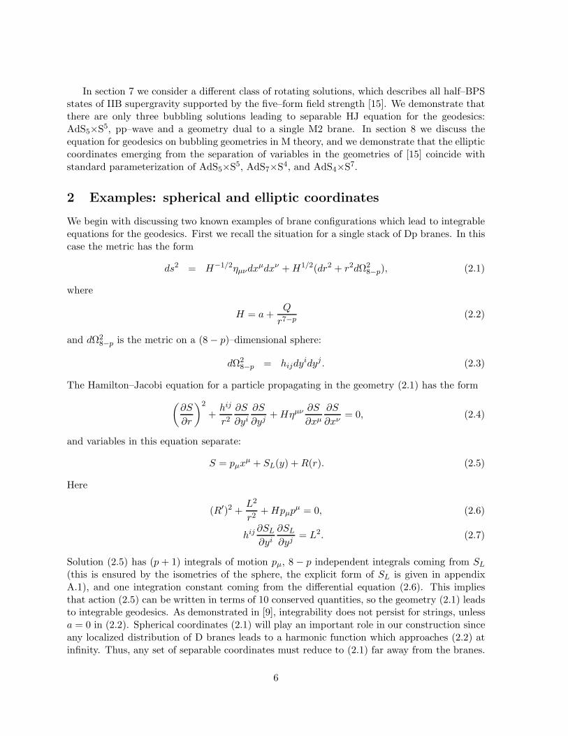
Section 3 describes our main procedure, which is subsequently used to study geodesics on avariety of backgrounds. In subsection 3.1 we demonstrate that the HJ equation (1.3) does notseparate unless the metric on the base space has the form
ds2base = dr21 + dr22 + r21dΩ2d1 + r22dΩ
2d2 , (1.6)
and H depends only on r1 and r2. The most general harmonic function H leading to integrableHJ equation is derived in section 3.2, and equations (3.50)-(3.52) summarize the main result ofthis paper for branes with flat worldvolume. The brane configurations giving rise to geometries(3.50)–(3.52) are analyzed in section 3.3. The results of section 3 imply that (Y0, . . . , Y10)leading to separation (1.4) must reduce to the elliptic coordinates discussed in section 2.
Section 4 discusses physical properties of the geometries leading to integrable geodesics. Wedemonstrate that separability persists for the wave equation beyond the eikonal approximation,a property that have been observed earlier for various black holes [18, 20]. In section 4.2 we showthat separability of the wave equation is associated with a hidden symmetry of the background,and we construct the conformal Killing tensor associated with this symmetry. In section 4.3we apply the techniques of [8, 9] to demonstrate that most backgrounds with separable waveequation do not lead to integrable string theories.
In section 5 our results are generalized to Dp–branes dissolved in D(p + 4)–branes, thesystem which plays an important role in understanding the physics of black holes [21]. We findthat in asymptotically–flat space there are no integrable solutions apart from the spherically–symmetric distribution of branes. However, there are several separable configurations in thenear–horizon limit of D(p+4)–branes, and the most general Dp–D(p+4) configurations leadingto separable HJ equation are presented in (5.17), (5.11).
In section 6 we consider another generalization by allowing the branes to rotate, i.e., bybreaking the Poincare symmetry on the brane worldvolume. Although the general analysisof rotating branes is beyond the scope of this paper, we consider the special class of rotatingsolutions which cover all microscopic states of the D1–D5 black hole [22, 23]. Such solutionsare parameterized by curves in eight–dimensional space, and our analysis demonstrates that HJequation is not separable unless this curve is a simple circle. For such configuration the separablecoordinates have been found before [24], and we will demonstrate that these coordinates reduceto a special case of the general elliptic coordinates discussed in section 3.2.
5In section 7 we will also discuss a special class of spherical branes.
5
In section 7 we consider a different class of rotating solutions, which describes all half–BPSstates of IIB supergravity supported by the five–form field strength [15]. We demonstrate thatthere are only three bubbling solutions leading to separable HJ equation for the geodesics:AdS5×S5, pp–wave and a geometry dual to a single M2 brane. In section 8 we discuss theequation for geodesics on bubbling geometries in M theory, and we demonstrate that the ellipticcoordinates emerging from the separation of variables in the geometries of [15] coincide withstandard parameterization of AdS5×S5, AdS7×S4, and AdS4×S7.
2 Examples: spherical and elliptic coordinates
We begin with discussing two known examples of brane configurations which lead to integrableequations for the geodesics. First we recall the situation for a single stack of Dp branes. In thiscase the metric has the form
ds2 = H−1/2ηµνdxµdxν +H1/2(dr2 + r2dΩ2
8−p), (2.1)
where
H = a+Q
r7−p(2.2)
and dΩ28−p is the metric on a (8− p)–dimensional sphere:
dΩ28−p = hijdy
idyj . (2.3)
The Hamilton–Jacobi equation for a particle propagating in the geometry (2.1) has the form
(
∂S
∂r
)2
+hij
r2∂S
∂yi∂S
∂yj+Hηµν
∂S
∂xµ∂S
∂xν= 0, (2.4)
and variables in this equation separate:
S = pµxµ + SL(y) +R(r). (2.5)
Here
(R′)2 +L2
r2+Hpµp
µ = 0, (2.6)
hij∂SL∂yi
∂SL∂yj
= L2. (2.7)
Solution (2.5) has (p + 1) integrals of motion pµ, 8 − p independent integrals coming from SL(this is ensured by the isometries of the sphere, the explicit form of SL is given in appendixA.1), and one integration constant coming from the differential equation (2.6). This impliesthat action (2.5) can be written in terms of 10 conserved quantities, so the geometry (2.1) leadsto integrable geodesics. As demonstrated in [9], integrability does not persist for strings, unlessa = 0 in (2.2). Spherical coordinates (2.1) will play an important role in our construction sinceany localized distribution of D branes leads to a harmonic function which approaches (2.2) atinfinity. Thus, any set of separable coordinates must reduce to (2.1) far away from the branes.
6
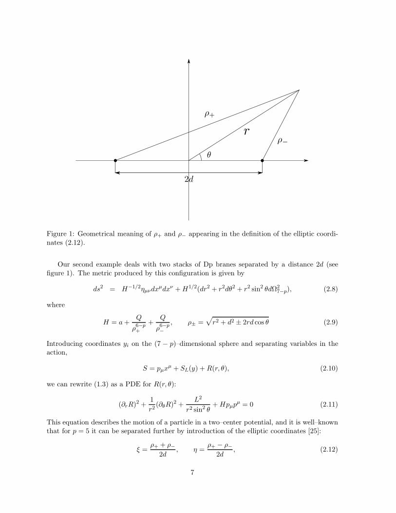
Figure 1: Geometrical meaning of ρ+ and ρ− appearing in the definition of the elliptic coordi-nates (2.12).
Our second example deals with two stacks of Dp branes separated by a distance 2d (seefigure 1). The metric produced by this configuration is given by
ds2 = H−1/2ηµνdxµdxν +H1/2(dr2 + r2dθ2 + r2 sin2 θdΩ2
7−p), (2.8)
where
H = a+Q
ρ6−p+
+Q
ρ6−p−
, ρ± =√
r2 + d2 ± 2rd cos θ (2.9)
Introducing coordinates yi on the (7 − p)–dimensional sphere and separating variables in theaction,
S = pµxµ + SL(y) +R(r, θ), (2.10)
we can rewrite (1.3) as a PDE for R(r, θ):
(∂rR)2 +
1
r2(∂θR)
2 +L2
r2 sin2 θ+Hpµp
µ = 0 (2.11)
This equation describes the motion of a particle in a two–center potential, and it is well–knownthat for p = 5 it can be separated further by introduction of the elliptic coordinates [25]:
ξ =ρ+ + ρ−
2d, η =
ρ+ − ρ−2d
, (2.12)
7
In appendix A.2 we review the separation procedure that leads to (2.10) and write down theexplicit form of R (see (A.16)). For future reference we quote the asymptotic relation betweenelliptic and spherical coordinates:
ξ =r
d+
d
2rsin2 θ +O
(
1
r3
)
, η = cos θ +d2
2r2cos θ sin2 θ +O
(
1
r4
)
. (2.13)
This completes our review of spherical and elliptic coordinates, and in the remaining partof this paper we will investigate whether the separation of variables persists for more generalgeometries produced by Dp–branes.
3 Geodesics in D–brane backgrounds
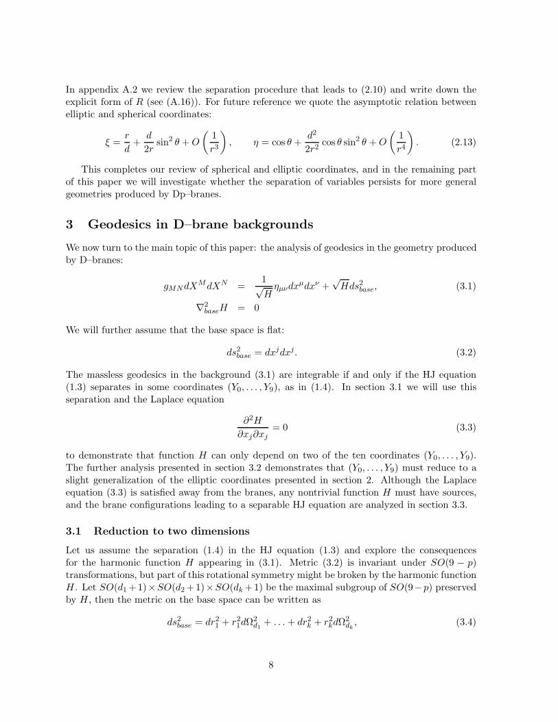
We now turn to the main topic of this paper: the analysis of geodesics in the geometry producedby D–branes:
gMNdXMdXN =
1√Hηµνdx
µdxν +√Hds2base, (3.1)
∇2baseH = 0
We will further assume that the base space is flat:
ds2base = dxjdxj. (3.2)
The massless geodesics in the background (3.1) are integrable if and only if the HJ equation(1.3) separates in some coordinates (Y0, . . . , Y9), as in (1.4). In section 3.1 we will use thisseparation and the Laplace equation
∂2H
∂xj∂xj= 0 (3.3)
to demonstrate that function H can only depend on two of the ten coordinates (Y0, . . . , Y9).The further analysis presented in section 3.2 demonstrates that (Y0, . . . , Y9) must reduce to aslight generalization of the elliptic coordinates presented in section 2. Although the Laplaceequation (3.3) is satisfied away from the branes, any nontrivial function H must have sources,and the brane configurations leading to a separable HJ equation are analyzed in section 3.3.
3.1 Reduction to two dimensions
Let us assume the separation (1.4) in the HJ equation (1.3) and explore the consequencesfor the harmonic function H appearing in (3.1). Metric (3.2) is invariant under SO(9 − p)transformations, but part of this rotational symmetry might be broken by the harmonic functionH. Let SO(d1+1)×SO(d2+1)×SO(dk+1) be the maximal subgroup of SO(9−p) preservedby H, then the metric on the base space can be written as
ds2base = dr21 + r21dΩ2d1 + . . .+ dr2k + r2kdΩ
2dk, (3.4)
8
and H becomes a function of (r1, . . . , rk). Moreover, since all rotational symmetries have beenisolated, we conclude that6
(ri∂j − rj∂i)H 6= 0. (3.5)
If the branes are localized in a compact region, then at sufficiently large values of
R =√
r21 + . . .+ r2k
function H satisfies the Laplace equation
1
rd11
∂
∂r1
[
rd11∂H
∂r1
]
+ . . . +1
rdkk
∂
∂rk
[
rdkk∂H
∂rk
]
= 0, (3.6)
and asymptotic behavior of function H is given by
H ∼ a+Q
(r21 + . . .+ r2k)q. (3.7)
Here a is a parameter, which is equal to zero for the near–horizon geometries and which can beset to one for asymptotically–flat solutions.
Our goal is to classify the backgrounds (3.1) that lead to separable HJ equations forgeodesics, and we begin with separating variables associated with symmetries. Poincare in-variance of (3.1) and rotational invariance of the base metric (3.4) allow us to write the actionappearing in the HJ equation (3.4) as
S = pµxµ +
k∑
i=1
S(di)Li
(Ωdi) + S(r1, . . . rk). (3.8)
Here pµ is the momentum of the particle in p + 1 directions longitudinal to the branes, and
S(di)Li
(Ωdi) is the part of the action that depends on coordinates y1, . . . , ydi of the sphere Ωdi .The label Li represents the angular momentum of a particle along this sphere, and it is definedby relation
hij∂SL∂yi
∂SL∂yj
= L2i . (3.9)
An explicit construction of S(d)L (Ω) is presented in appendix A.1.
Substitution of (3.8) in the HJ equation (1.3) leads to equation for S:
k∑
i=1
(
∂S
∂ri
)2
+L2i
r2i
+Hpµpµ = 0. (3.10)
A special case of this equation with k = 1 separates in spherical coordinates (see section 2),and we will now prove the equation (3.10) does not separate if k > 2. The separation of (3.10)for k = 2 will be discussed in section 3.2.
6If this relation is not satisfied for i = 1, j = 2, then SO(d1 +1)×SO(d2 +1) is enhanced to SO(d1 + d2+2).
9
Separability of equation (3.10) should persist for all values of angular momenta, so we beginwith setting all Lj to zero and p1 = . . . = pp = 0. The resulting equation (3.10) can be viewedas a HJ equation on an effective (k + 1)–dimensional space
ds2 = −H−1dt2 + dr21 + . . .+ dr2k (3.11)
A general theory of separable HJ equations on curved backgrounds has a long history (see [26]),and a complete classification is presented in [27, 28]. In particular, this theory distinguishesbetween ignorable directions (which correspond to Killing vectors) and non-ignorable ones.Clearly, the time direction in (3.11) is ignorable, but (3.11) does not have additional Killingvectors which commute with ∂t. Indeed, any such vector would be a Killing vector of the k–dimensional flat space, so it must be a combination of translations and rotations in ri. However,the asymptotic behavior of function H (3.7) breaks translational symmetry, and our assump-tion (3.5) destroys the rotational Killing vectors, so if the HJ equation for the metric (3.11)separates in some coordinates (t, x1, . . . xk), only one of them (specifically, t) can correspondto an ignorable direction. Moreover, the discrete symmetry t → −t of (3.11) guarantees that tdoes not mix with (x1, . . . xk) in the metric, and such orthogonality leads to simplifications inthe general analysis of [27, 28].
Specifically, according to theorem 6 of [28] separation of variables in (3.11) implies that7
(1) There exist k independent conformal Killing tensors A(a) with components (A(a)ij , A
(a)tt ).
(2) Each of the one–forms dxl = ωlidri is a simultaneous eigenform of all Aij(a) with eigenvalues
ρ(a,l). This implies that a projector P (l)ij onto dx
l satisfies equation
(Aij(a) − ρ(a,l)gij)P (l)j
k = 0. (3.12)
(3) The metric in coordinates dxl is diagonal, so projectors P (l)ij commute with Aij
(a)and
gij , and projectors with different values of l project onto orthogonal subspaces. Since thenumber of projectors is equal to the number of coordinates, we arrive at the decomposition
Aij(a) =
k∑
l
ρ(a,l)hlPij(l), gij =
k∑
l
hlPij(l) (3.13)
(4) The components of A(a) along the Killing direction satisfy an overdefined system of differ-ential equations:
∂i
[
Att(a)
]
−k∑
l
ρ(a,l)Pi(l)j∂jg
tt = 0 (3.14)
Notice that in [28] the theorem is formulated in terms of coordinates xi, so it does not usethe projectors. For our purposes the covariant formulation given above is more convenient, inparticular, to rule our the separation of variables, we will have to work in the original coordinates
7The discussion of [27, 28] is more general: it allows mixing between ignorable and essential coordinates.
10
ri and demonstrate that the required Killing tensors A(a) do not exist. Notice that equation(3.14) can be rewritten in the form which does not refer to projectors (and thus to coordinatesxi): multiplying this equation by gij and using (3.13), we find
gij∂j(Att(a))−Aij(a)∂jg
tt = 0. (3.15)
This relation is equivalent to (tti) component of the equation for the Killing tensor A(a).
The theorem quoted above implies that A(a)ij are conformal Killing tensors on the k–dimensional
base of (3.11), and, for the flat base, all such tensors can be written as quadratic combinationsof k(k + 3)(k + 4)(k + 5)/12 Killing vectors [29]8:
A(a)ij =
∑
m,n
b(a)m,nV(m)i V
(n)j (3.16)
Equations (3.12) and (3.15) give severe restrictions on coefficients b(a)m,n, but fortunately the
consequences of (3.12) have been analyzed elsewhere. Indeed, equation (3.12) does not involvegtt, so it remains the same for H = 1, when (3.11) gives the flat space, and the correspondingHJ equation gives an eikonal approximation for the standard wave equation. It is well-knownthat in 3 + 1 dimensions (k = 3) the latter can only be separated in ellipsoidal coordinatesand their special cases [26], and generalization of this result to k > 3 is presented in [27, 28].This leads to the conclusion that the HJ equation in the metric (3.11) with k > 2 can onlyseparate in ellipsoidal coordinates or in the degenerate form thereof. Before ruling out thispossibility, we briefly comment on the peculiarities of the two–dimensional base. In this casethe conformal group becomes infinite-dimensional, so the base space admits an infinite numberof the conformal Killing tensors. This situation will be analyzed in section 3.2.
To summarize, we concluded that for k > 2, the HJ equation can only be separable in somespecial case of ellipsoidal coordinates (x1, . . . , xk), which are defined by [30, 31]
r2i = −
∏
j
(a2i + xj)
∏
j 6=i
1
(a2j − a2i )
. (3.17)
Here (a1, . . . , ak) is the set of positive constants, which specify the ranges of variables xi:
x1 ≥ −a21 ≥ x2 ≥ −a22 ≥ . . . xk ≥ −a2k, (3.18)
Rewriting the metric (3.11) in terms of xi and substituting the result into (3.10), we find theHJ equation in ellipsoidal coordinates (see appendix B for detail):
k∑
i=1
1
h2i
(
∂S
∂xi
)2
+L2i
r2i
+Hpµpµ = 0. (3.19)
Here hi is defined by
h2i =1
4
∏
j 6=i
(xi − xj)
∏
j
1
a2j + xi
. (3.20)
8The explicit form of the conformal Killing vectors is given in appendix D.2.
11
Function H appearing in (3.19) must satisfy equation (3.6) away from the sources, and ap-pendix B we demonstrate that for such functions equation (3.19) never separates in ellipsoidalcoordinates. This shows that the HJ equation can only be integrable for k = 1 (the situationconsidered in section 2) and for k = 2, which will be analyzed in the next subsection.
3.2 Separation of variables and elliptic coordinates
In the last subsection we have demonstrated that the HJ equation (3.10) is not integrable unlessthe flat base has the form (3.4) with k ≤ 2 and H is a function of r1 and r2 only. In section 2we have already discussed k = 1 and this subsection is dedicated to the analysis of k = 2. Tosimplify some formulas, we slightly deviate from the earlier notation and write the metric (3.1)with the base (3.4) for k = 2 as
ds2 =1√Hηµνdx
µdxν +√H(dr2 + r2dθ2 + r2 cos2 θdΩ2
m + r2 sin2 θdΩ2n), (3.21)
The connection to coordinates of (3.4) is obvious:
r1 = r cos θ, r2 = r sin θ, (3.22)
with d1 = m,d2 = n. The arguments presented in the last subsection ensure that H appearingin (3.21) can only depend on r and θ, i.e., the distribution of Dp branes that sources thisharmonic function is invariant under SO(m+ 1)× SO(n+ 1) rotations. Notice that
p = 7−m− n. (3.23)
The Poincare and SO(m+1)×SO(n+1) symmetries of (3.21) lead to a partial separationof the Hamilton–Jacobi equation (1.3) for geodesics (this equation is a counterpart of (3.8)):
S = pµxµ + S
(m)L1
(y) + S(n)L2
(y) +R(r, θ), (3.24)
where S(m)L1
and S(n)L2
satisfy differential equations
hij∂S
(m)L1
∂yi∂S
(m)L1
∂yj= L2
1, hij∂S
(n)L2
∂yi∂S
(n)L2
∂yj= L2
2, (3.25)
and L1, L2 are angular momenta on the spheres. An explicit solution of equations (3.25) ispresented in appendix A.1.
Substitution of (3.24) into (1.3) leads to the equation for R(r, θ):
(∂rR)2 +
1
r2(∂θR)
2 +L21
r2 cos2 θ+
L22
r2 sin2 θ+ pµp
µH(r, θ) = 0. (3.26)
We recall that H(r, θ) is a harmonic function describing the distribution of D branes, so awayfrom the sources it satisfies the Laplace equation on the base of the ten–dimensional metric(3.21):
1
rm+n+1∂r(r
m+n+1∂rH) +1
r2 sinn θ cosm θ∂θ(sin
n θ cosm θ∂θH) = 0. (3.27)
12
Let us assume that the massless HJ equation (3.26) separates in coordinates (x1, x2). Inparticular, this implies that the metric in (x1, x2) must have a form [32, 33]
dr2 + r2dθ2 = A(x1, x2)[
eg1(dx1)2 + eg2(dx2)
2]
, (3.28)
where g1(x1, x2) and g2(x1, x2) satisfy the Stackel conditions:
∂j∂igl − ∂jgl ∂igl + ∂jgl ∂igj + ∂igl ∂jgi = 0, i 6= j (3.29)
We wrote the Stackel conditions (3.29) for an arbitrary number of coordinates to relate to ourdiscussion in section 3.1, but in the present case (k = 2) equation (3.29) gives only two relations(i = 1, j = 2, l = 1, 2):
∂2∂1g1 + ∂2g1 ∂1g2 = 0, ∂2∂1g2 + ∂1g2 ∂2g1 = 0 (3.30)
In particular, we find that
g1 − g2 = f1(x1)− f2(x2), (3.31)
so by adjusting function A in (3.28) we can set
g1 = f1(x1), g2 = f2(x2). (3.32)
We can further redefine variables, x1 → x1(x1), x2 → x2(x2) to set g1 = g2 = 0, at least locally.9
Introducing x = x1, y = x2, we rewrite (3.28) as
dr2 + r2dθ2 = A(x, y)[
dx2 + dy2]
. (3.33)
To summarize, we have demonstrated that in two dimensions the Stackel conditions (3.29) implythat coordinates xi separating the HJ equation are essentially the same as the conformally–Cartesian coordinates (x, y) in (3.33)10. In higher dimensions, conditions (3.29) are less strin-gent than the requirement for coordinates xi to be conformally–Cartesian: for example, condi-tions (3.29) are satisfied by spherical coordinates that have
g1 = 0, g2 = 2 lnx1, g2 = 2 ln(x1 sinx2), (3.34)
but there is no change of coordinates of the form xi(xi) that allows one to write
(dx1)2 + x21dx
22 + [x1 sinx2]
2(dx3)2 = A
∑
(dxi)2. (3.35)
Moreover, for k > 2, a relation
k∑
i=1
(dri)2 = A
k∑
i=1
(dxi)2 (3.36)
9Notice that separation in variables (x1, x2) implies separation in (x1, x2).10Although any two–dimensional metric can be written as A[(dx1)
2 +(dx2)2] in some coordinates, a priori the
HJ equation does not have to separate in (x1, x2). It is the Stackel conditions (3.30) that guarantee that any setof separable coordinates can be rewritten in a conformally–flat form without destroying the separation.
13
implies that A must be equal to constant, so if conformally–Cartesian coordinates xi separatethe HJ equation, then xi must be Cartesian11.
Returning to k = 2, we will now find restrictions on A(x, y) and H(r, θ). First we defineR(x, y) by
R(x, y) ≡ R(r, θ). (3.37)
Then equation (3.33) can be used to rewrite (3.26) in terms of R, and we find the necessaryand sufficient conditions for the Hamilton–Jacobi equation (3.26) to be separable:
(∂rR)2 +
1
r2(∂θR)
2 =1
A(x, y)
[
(∂xR)2 + (∂yR)
2]
, (3.38)
L21
r2 cos2 θ+
L22
r2 sin2 θ−M2H(r, θ) =
1
A(x, y)[U1(x) + U2(y)] . (3.39)
Here M is an effective mass in (p + 1) dimensions defined by
M2 = −pµpµ. (3.40)
The construction of the most general harmonic function H(r, θ) that admits the separationof variables (3.38)–(3.39) will be performed in three steps:
1. Determine the restrictions on function A(x, y) imposed by equation (3.38).
2. Use equation (3.39) to find H(r, θ) corresponding to a given A(x, y). (3.41)
3. Use the Laplace equation (3.27) to find further restrictions on A(x, y).
To implement the first step, it is convenient to introduce complex variables
z = x+ iy, w = lnr
l+ iθ. (3.42)
Here l is a free parameter which has dimension of length. Rewriting equation (3.38) in termsof complex coordinates,
∂wR∂wR =l2ew+w
A∂zR∂zR. (3.43)
we conclude that12
∂z
∂w
∂z
∂w= 0, (3.44)
so z(w, w) is either holomorphic or anti–holomorphic. Without loss of generality we assumethat
z = h(w), (3.45)
11To see this, one has to evaluate the Riemann tensor for both sides of (3.36).12The alternative solution, ∂zR = ∂zR = 0, leads to R = R = const, which does not solve (3.26).
14
then equation (3.43) gives an expression for A(x, y):
A =l2ew+w
|h′|2 =r2
|h′|2 (3.46)
The second step amounts to rewriting equation (3.39) as
H(r, θ) =1
M2
[
L21
r2 cos2 θ+
L22
r2 sin2 θ− |h′|2
r2
[
U1
(
h+ h
2
)
+ U2
(
h− h
2i
)]]
. (3.47)
Implementation of the third step amounts to finding expressions for h(w) and U1(x), U2(y)which are consistent with Laplace equation (3.27) for function H. Physically interesting con-figurations correspond to branes distributed in a compact spacial region, so at large values of rfunction H behaves as
H = a+Q
r7−p+O(rp−8). (3.48)
Here Q is the total brane charge, and a is a parameter, which can be set to zero for asymptoti-cally flat space, and which is equal to zero for the near–horizon geometry of branes (cf. equation(2.2)). Keeping only the two leading terms in (3.48), we conclude that the Hamilton–Jacobiequation (3.26) separates in coordinates (r, θ), and the solution is similar to the first examplediscussed in section 2. The subleading corrections in (3.48) obstruct the separation in sphericalcoordinates, but for some harmonic functions H the Hamilton–Jacobi equation (3.26) separatesin a different coordinate system, as in the second example discussed in section 2. Notice thatat large values of r the new coordinate system must approach spherical coordinates since (3.48)depends only on r, and for elliptic coordinates such asymptotic reduction was given by equation(2.13).
In appendix C we construct the most general expressions for h(w), U1(x), U2(y) by startingwith asymptotic relations (3.48) and
z = w +O
(
l
r
)
, (3.49)
and writing expansions in powers of l/r. Notice that these asymptotics lead to the unique valueof l for a given configuration of branes (for example, l = d/2 in (3.55)). Requiring that function(3.47) satisfies the Laplace equation (3.27), the boundary condition (3.48), and remains regularat sufficiently large r, we find three possible expressions for h and U1, U2:
13
I : h(w) = w, H =Q
rm+n, U1(r) = − QM2
rm+n−2, U2(θ) =
L21
cos2 θ+
L22
sin2 θ. (3.50)
II : h(w) = ln
[
1
2
ew +√
e2w − 4
]
, H =1
(cosh2 x− cos2 y)
Q
sinhn−1 x coshm−1 x.
13To avoid unnecessary complications in (3.50)–(3.53) we set a = 0 in these expressions, but constant a canbe added to the harmonic function without destroying the separation (3.39). This leads to minor changes in U1
and U2.
15
U1(x) = − Q(Md)2
sinhn−1 x coshm−1 x− L2
1
cosh2 x+
L22
sinh2 x, U2(y) =
L21
cos2 y+
L22
sin2 y. (3.51)
III : h(w) = ln
[
1
2
ew +√
e2w + 4
]
, H =1
(cosh2 x− sin2 y)
Q
sinhm−1 x coshn−1 x.
U1(x) = − Q(Md)2
sinhm−1 x coshn−1 x− L2
2
cosh2 x+
L21
sinh2 x, U2(y) =
L21
cos2 y+
L22
sin2 y. (3.52)
The derivation of these constraints is presented in appendix C.For six– and seven–branes14 (i.e., for m+n < 2), harmonic function is slightly more general:
I : H = − 1
M2r2
[
C1
rm+n−2+
C3
sinn−1 θ cosm−1 θ
+C4
sinn−1 θF
(
m− 1
2,3− n
2,m+ 1
2; cos2 θ
)]
II : H =1
(cosh2 x− cos2 y)
[
Q
sinhn−1 x coshm−1 x+
P
sinm−1 y cosn−1 y
]
, (3.53)
III : H =1
(cosh2 x− sin2 y)
[
Q
sinhm−1 x coshn−1 x+
P
cosm−1 y sinn−1 y
]
.
The terms proportional to P are ruled out by the boundary condition (3.48) for p < 6, but theyare allowed for p = 6, 7.
Notice that case III can be obtained from case II by interchanging the spheres Sm and Sn,so, without loss of generality, we can focus on solutions I and II. Case I corresponds to sphericalcoordinates, and case II corresponds to elliptic coordinates discussed in the second example ofsection 2: as demonstrated in appendix C, expression (3.51) for h(w),
h(w) = ln
[
1
2
ew +√
e2w − 4
]
, (3.54)
is equivalent to
cosh x =ρ+ + ρ−
2d, cos y =
ρ+ − ρ−2d
, ρ± =√
r2 + d2 ± 2rd cos θ, d = 2l. (3.55)
Thus (x, y) are equivalent to the elliptic coordinates (ξ, η) defined by (2.12). For future refer-ence, we rewrite the metric (3.21) in terms of x and y (see (C.12)):
ds2 =1√Hηµνdx
µdxν +√Hds2base, (3.56)
ds2base = 4l2[
(cosh2 x− cos2 y)(dx2 + dy2) + sinh2 x sin2 ydΩ2n + cosh2 x cos2 ydΩ2
m
]
.
14Condition (3.23) as well as restrictions m,n ≥ 0 imply that ansatz (3.21) covers only p ≤ 7
16
3.3 Properties of the brane sources
In section 3.2 we have classified the geometries which lead to separable Hamilton–Jacobi equa-tions for geodesics. The Laplace equation (3.27) played an important role in our construction,but this equation is only satisfied away from the sources. In this subsection we will analyzethe solutions (3.50)–(3.52) to find the sources of the Poisson equation and to identify the cor-responding distribution of branes. As already discussed in section 2, the spherically symmetricdistribution (3.50) corresponds to a single stack of Dp branes.
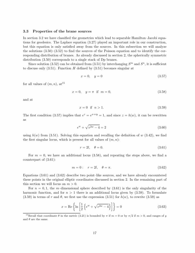
Since solution (3.52) can be obtained from (3.51) by interchanging Sm and Sn, it is sufficientto discuss only (3.51). Function H defined by (3.51) becomes singular at
x = 0, y = 0 (3.57)
for all values of (m,n), at15
x = 0, y = π if m = 0, (3.58)
and at
x = 0 if n > 1. (3.59)
The first condition (3.57) implies that ez = ex+iy = 1, and since z = h(w), it can be rewrittenas
ew +√
e2w − 4 = 2 (3.60)
using h(w) from (3.51). Solving this equation and recalling the definition of w (3.42), we findthe first singular locus, which is present for all values of (m,n):
r = 2l, θ = 0. (3.61)
For m = 0, we have an additional locus (3.58), and repeating the steps above, we find acounterpart of (3.61):
m = 0 : r = 2l, θ = π. (3.62)
Equations (3.61) and (3.62) describe two point–like sources, and we have already encounteredthese points in the original elliptic coordinates discussed in section 2. In the remaining part ofthis section we will focus on m > 0.
For n = 0, 1, the m–dimensional sphere described by (3.61) is the only singularity of theharmonic function, and for n > 1 there is an additional locus given by (3.59). To formulate(3.59) in terms of r and θ, we first use the expression (3.51) for h(w), to rewrite (3.59) as
x = Re
ln
[
1
2
ew +√
e2w − 4
]
= 0 (3.63)
15Recall that coordinate θ in the metric (3.21) is bounded by π if m = 0 or by π/2 if m > 0, and ranges of yand θ are the same.
17
(a) m = 0, n ≤ 1 (b) m = 0, n > 1
(c) m > 0, n ≤ 1 (d) m > 0, n > 1
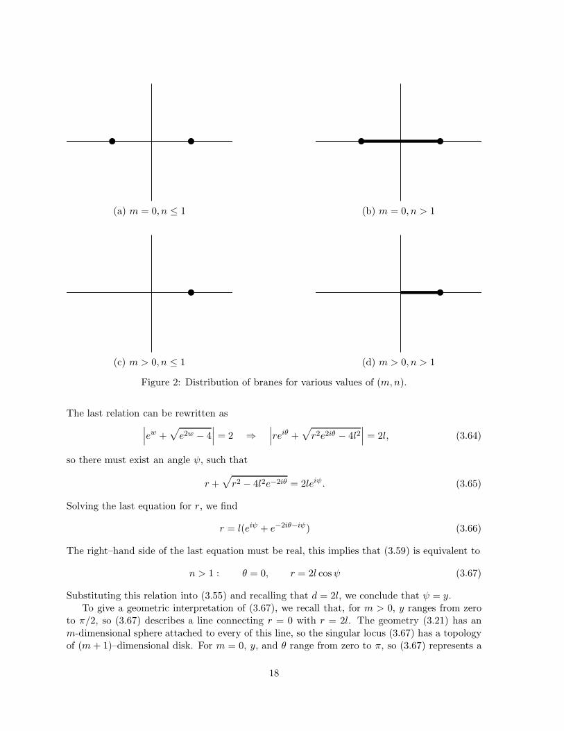
Figure 2: Distribution of branes for various values of (m,n).
The last relation can be rewritten as∣
∣
∣ew +
√
e2w − 4∣
∣
∣= 2 ⇒
∣
∣
∣reiθ +
√
r2e2iθ − 4l2∣
∣
∣= 2l, (3.64)
so there must exist an angle ψ, such that
r +√
r2 − 4l2e−2iθ = 2leiψ. (3.65)
Solving the last equation for r, we find
r = l(eiψ + e−2iθ−iψ) (3.66)
The right–hand side of the last equation must be real, this implies that (3.59) is equivalent to
n > 1 : θ = 0, r = 2l cosψ (3.67)
Substituting this relation into (3.55) and recalling that d = 2l, we conclude that ψ = y.To give a geometric interpretation of (3.67), we recall that, for m > 0, y ranges from zero
to π/2, so (3.67) describes a line connecting r = 0 with r = 2l. The geometry (3.21) has anm-dimensional sphere attached to every of this line, so the singular locus (3.67) has a topologyof (m+ 1)–dimensional disk. For m = 0, y, and θ range from zero to π, so (3.67) represents a
18
line connecting two singular points (3.61), (3.62). The pictorial representation of singular lociin (r, θ) plane is given in figure 2.
We will now combine (3.61) and (3.67) to analyze the brane distribution for m > 0.
(a) n = 0.In this case, the m–dimensional sphere described by (3.61) is the only singularity of theharmonic function, and in the vicinity of this singularity we find
H =Qx
x2 + y2+ regular (3.68)
To give a geometric interpretation of this expression, we consider the base metric (3.21) inthe vicinity of singularity (3.61):
ds29−p ≈ (2l)2dΩ2m + dr2 + (2l)2dθ2. (3.69)
It is convenient to introduce polar coordinates (R,Φ) by
r = 2l +R cos Φ, 2lθ = R sinΦ. (3.70)
Recalling that θ varies from −π2 to π
2 when n = 0, we conclude that Φ ∈ [0, 2π) (orΦ ∈ [−π, π), see below), as long as R remains small. Then metric (3.69) takes the standardform
ds29−p ≈ (2l)2dΩ2m + dR2 +R2dΦ2. (3.71)
To write (x, y) in terms of (R,Φ), we use the real form (3.55) of the holomorphic map(3.51). In particular, for small x and y we find
x2 + y2 ≈ 2(cosh x− cos y) =2ρ−2l
=2
2l
√
(r − 2l)2 + 4rl(1− cos θ) ≈ R
l(3.72)
x2 ≈ 2(cosh x− 1) ≈ 1
2l
[
(r − 2l) +√
(r − 2l)2 + 4rl(1− cos θ)]
≈ R
lcos2
Φ
2.
Extraction of the square root from the last expression should be done carefully: positivityof the harmonic function (3.68) (or (3.51)) requires that x > 0. Thus we can write
x =
√
R
lcos
Φ
2, (3.73)
as long as Φ ∈ [−π, π). The range Φ ∈ [0, 2π) is equivalent from the point of view of (3.70),but it leads to a more complicated counterpart of (3.73), and it will not be explored further.Substitution of (3.72) and (3.73) into equation (3.68) leads to a simple expression for theharmonic function in the vicinity of the sources:
H = Q
√
l
Rcos
Φ
2+ regular (3.74)
We recall that R = 0 corresponds to them–dimensional sphere (3.61) with radius 2l. Noticethat this expression never becomes negative since Φ ∈ [−π, π).
19
(b) n = 1.Here again, the m–dimensional sphere described by (3.61) is the only singularity of theharmonic function, and in the vicinity of this singularity we find
H =A
x2 + y2+ regular =
Al
R+ regular (3.75)
As before, we used (3.72) to rewrite the harmonic function in terms of coordinates (3.70),and in this case
ds29−p ≈ (2l)2dΩ2m + dR2 +R2dΦ2 +R2 sin2 Φdφ2, 0 ≤ Φ < π
Formula (3.75) gives a standard harmonic function in three dimensions transverse to Sm,so this configuration corresponds to D–branes uniformly distributed over Sm.
(c) n > 1.In this case the singularity consists of a line (3.67) connecting r = 0 and (3.61) with sphereSm fibered over it. In the vicinity of θ = 0, the base of the metric (3.21) becomes
ds29−p ≈ dr2 + r2dΩ2m + r2dθ2 + r2θ2dΩ2
n, (3.76)
and the locus (3.67) is an m+ 1–dimensional ball with metric
ds2sing ≈ dr2 + r2dΩ2m, 0 ≤ r < 2l (3.77)
The singularity corresponds to x = 0 (recall (3.57) and (3.59)), and the leading contributionto the harmonic function (3.51) for small x is
H =1
x2 + sin2 y
Q
xn−1+ . . . (3.78)
For small x, metric (3.56) becomes
ds2base ≈ 4l2 cos2 ydΩ2m + 4l2(x2 + sin2 y)
[
dx2 + dy2]
+ 4l2x2 sin2 ydΩ2n. (3.79)
Away from y = 0, we can neglect x2 in comparison with sin2 y, then function (3.78) describesthe Coulomb potential produced by D–branes uniformly distributed over Sm. Rewriting(3.79) as
ds2base ≈ dR2 +R2dΩ2m + (4l2 −R2)
[
dx2 + x2dΩ2n
]
, (3.80)
we find the charge density ρ:
H =ρ
[(4l2 −R2)x2](n−1)/2+ . . . ,
ρ = 4l2Q(4l2 −R2)n−3
2 = (2l)n−1Q sinn−3 y (3.81)
As expected, the charge density vanishes on the boundary (3.61) of the ball, where y = 0.
To summarize, we found that for n ≤ 1 the brane sources are localizes on the m–dimensionalsphere, they produce a Coulomb potential (3.75) for n = 1 and a potential (3.74) with afractional power of the radial coordinate R for n = 0. For n > 1, the branes are located on aline connecting r = 0 and (3.61) with sphere Sm fibered over it ((R,Ωm) subspace of (3.80)).These sources produce a Coulomb potential in (n+1) transverse directions with charge density(3.81).
20
4 Beyond geodesics: wave equation, Killing tensors, and strings
The main goal of this paper is identification of backgrounds which can potentially lead tointegrable string theories. As discussed in the introduction, integrability can be ruled out bylooking at relatively simple equations for the light modes of strings (massless particles), andin the last section we demonstrated that classical equations of motion for such particles areintegrable only for the harmonic functions given by (3.50)–(3.52). It is natural to ask whetherseparability of the HJ equation (1.3) in the elliptic coordinates (3.55) persists at the quantumlevel and whether it is related to some hidden symmetry of the system. In section 4.1 weanalyze integrability of the wave equation, a quantum counterpart of (1.3), and in section 4.2we identify the Killing tensor responsible for the separation. Finally in section 4.3 we investigatethe question whether integrability of geodesics persists for finite size strings.
4.1 Separability of the wave equation
In this subsection we will analyze the wave equation which governs dynamics of a minimally–coupled massless scalar:
1√−g ∂M(
gMN√−g∂NΨ)
= 0. (4.1)
Most Dp–branes generate a nontrivial dilaton, so the last equation would look differently in thestring and in the Einstein frames16, and here we will focus on the most interesting case of theEinstein frame:
g(E)MNdx
MdxN = e−Φ/2
[
1√Hηµνdx
µdxν +√Hds2base
]
, e2Φ = H(3−p)/2. (4.2)
Since the HJ equation (1.3) arises in the eikonal approximation of (4.1), the arguments presentedin sections 3 imply that (4.1) is not integrable unless the metric ds2base has the form (3.56) andH is given by (3.51)17, although these conditions are not sufficient for integrability of (4.1)18.
To write the wave equation in the geometry (4.2), we recall the metric on the base (3.56),
ds2base = (cosh2 x− cos2 y)(dx2 + dy2) + sinh2 x sin2 ydΩ2n + cosh2 x cos2 ydΩ2
m, (4.3)
and introduce a convenient notation:
A = (cosh2 x− cos2 y), X = sinhn x coshm x, Y = sinn y cosm y. (4.4)
Evaluating the determinant of the metric,
√
−g(E) = e−5Φ/2H2−p/2X(x)Y (y)A, (4.5)
16Unlike (4.1), the HJ equation (1.3) is invariant under conformal rescaling of the metric, so the results ofsection 3 are valid in both the string and the Einstein frames.
17Solution (3.50) leads to a trivial separation in spherical coordinates, and solution (3.52) reduces to (3.51).18For example, as we will see below, equation (4.1) does not separate if gMN is a metric in the string frame,
although it still reduces to (1.3) in the eikonal approximation.
21
and substituting (4.2), (4.3), (4.5) into (4.1), we find the wave equation:
H∂µ∂µΨ+
1
sinh2 x sin2 y∆ΩnΨ+
1
cosh2 x cos2 y∆ΩmΨ
+H(p−3)/2e2Φ
AXY
∂x
[
H(3−p)/2e−2ΦXY ∂xΨ]
+ ∂y
[
H(3−p)/2e−2ΦXY ∂yΨ]
= 0 (4.6)
This equation separates since H(3−p)/2e−2Φ = 1 (see (4.2)). Specifically, if we write19
Ψ = eipµxµ
Yk(Ωm)Yl(Ωn)F (x)G(y), (4.7)
then (4.6) splits into two ordinary differential equations with separation constant Λ:
[
−(
a cosh2 x+Q
sinhn−1 x coshm−1 x
)
pµpµ − l(l + n− 1)
sinh2 x+k(m+ k − 1)
cosh2 x
]
F
+1
X
[
XF ′]′= ΛF (4.8)
apµpµ cos2 y −
[
l(l + n− 1)
sin2 y+k(m+ k − 1)
cos2 y
]
G+1
Y
[
Y G′]′= −ΛG (4.9)
We used the expression for the harmonic function,
H = a+1
(cosh2 x− cos2 y)
Q
sinhn−1 x coshm−1 x(4.10)
found in section 3 (see (3.51), (3.52)).Let us now demonstrate that the wave equation (4.1) does not separate in the string metric
unless p = 3. The string–frame counterpart of (4.6) can be obtained by formally setting e2Φ = 1in that equation:
H∂µ∂µΨ+
1
sinh2 x sin2 y∆ΩnΨ+
1
cosh2 x cos2 y∆ΩmΨ
+H(p−3)/2
AXY
∂x
[
H(3−p)/2XY ∂xΨ]
+ ∂y
[
H(3−p)/2XY ∂yΨ]
= 0 (4.11)
Clearly, the multiplicative separation (4.7) does not work for this equation unless p = 3. Sincecoordinates (x, y) are uniquely fixed by the discussion of the HJ equation (which is an eikonallimit of (4.11)) presented in section 3, to rule out the separation, it is sufficient to show that asubstitution of
Ψ = eipµxµ
Yk(Ωm)Yl(Ωn)F (x)G(y)P (x, y) (4.12)
19Here Yk(Ωm) and Yl(Ωn) are standard spherical harmonics with angular momenta k and l. For example,∆Ωn
Yl(Ωn) = −l(l + n− 1)Yl(Ωn).
22
into (4.11) does not lead to separate equations for F and G for any fixed function P (x, y). Todemonstrate this, we perform such substitution and rewrite the result as
−A[
Hpµpµ +
l(l + n− 1)
sinh2 x sin2 y+k(k +m− 1)
cosh2 x cos2 y
]
+H(p−3)/2
P
1
X∂x
[
H(3−p)/2X∂xP]
+1
Y∂y
[
H(3−p)/2Y ∂yP]
+1
F
F ′′ + F ′∂x ln[
H(3−p)/2XP 2]
(4.13)
+1
G
G′′ +G′∂y ln[
H(3−p)/2Y P 2]
= 0
Since H and P are fixed functions, the first two lines of (4.13) remain the same for all F andG, so equation (4.13) does not separate unless its third line is only a function of x and the forthline is only a function of y. This implies that
∂x∂y ln[
H(3−p)/2P 2]
= 0 ⇒ P = H(p−3)/4P1(x)P2(y). (4.14)
Functions P1 and P2 can be absorbed into F and G (recall (4.12)), so we set P1 = P2 = 1.Direct substitution into (4.13) shows that the third line of that equation obstructs separationunless p = 3.
To summarize, we have demonstrated that while the HJ equation is integrable in the ellipticcoordinates (3.55), its quantum version may or may not be separable depending on the frame.In particular, the equation for the minimally–coupled massless scalar separates in the Einstein,but not in the string frame.
4.2 Killing tensor
Separation the Hamilton–Jacobi and Klein–Gordon equations implies an existence of nontrivialconserved charges which are associated with symmetries of the background. In the simplestcase, such symmetries are encoded in the Killing vectors, which correspond to invariance of themetric under reparametrization
xM → xM + VM (x), (4.15)
where VM (x) satisfies the equation
VM ;N + VN ;M = 0. (4.16)
This symmetry guarantees a conservation of the charge
QV = VM ∂S
∂xM, (4.17)
and momenta pµ appearing in (3.8) were examples of such charges. Although not every separa-tion of variables can be associated with Killing vector (separation between x and y coordinatesfound in sections 3 and 4.1 is our prime example), the general theory developed in [18, 27, 28, 34]
23
guarantees that any such separation is related to a symmetry of the background, which is en-coded by a (conformal) Killing tensor. In this subsection we will discuss the conformal Killingtensor associated with separation (3.51) and (4.8)–(4.9).
The conformal Killing tensor of rank two satisfies equation
∇(MKNL) =1
2W(MgNL), (4.18)
which is solved in appendix D. Here we will deduce the same solution by using the separationof variables found in section 3. A conformal Killing tensor KMN always implies that
I = KMN∂MS∂NS (4.19)
is an integral of motion of the massless HJ equation20, so KMN can be extracted from the knowseparation. Going to the eikonal approximation in (4.6) with harmonic function (4.10), we find
[
a cosh2 x+Q
sinhn−1 x coshm−1 x
]
∂µS∂µS +
1
sinh2 xhij∂iS∂jS
− 1
cosh2 xhij ∂iS∂jS + ∂xS∂xS (4.20)
= −a∂µS∂µS − 1
sin2 yhij∂iS∂jS − 1
cos2 yhij ∂iS∂jS − ∂yS∂yS
For separable solutions, both sides of this equation must be constant, and identifying thisconstant with −I in (4.19), we find
KMNpMpN = apµpµ +
1
sin2 yhijpipj +
1
cos2 yhij pipj + pypy (4.21)
In appendix D this expression is derived in a geometrical way by solving the equation (4.18)for the Killing tensor.
4.3 Non–integrability of strings
In section 3 we have classified all supersymmetric configurations of Dp–branes that lead tointegrable equations for null geodesics. Specifically, we demonstrated that a metric (3.1)–(3.2)leads to a separable HJ equation (1.3) if and only if it has the form
ds2 =1√Hηµνdx
µdxν +√H(dr2 + r2dθ2 + r2 cos2 θdΩ2
m + r2 sin2 θdΩ2n) (4.22)
with the harmonic function H from (3.50)–(3.52). In this subsection we will investigate whetherintegrability of geodesics extends to strings with finite size. Our discussion will follow the logicpresented in [9], and to compare our results with ones from that paper we rewrite the metricin terms of a new function f = H1/4 so the metric (4.22) becomes:
ds2 =1
f2ηµνdx
µdxν + f2(dr2 + r2dθ2 + r2 cos2 θdΩ2m + r2 sin2 θdΩ2
n). (4.23)
20A Killing tensor KMN , which has VM = 0 in (4.18), implies that (4.19) is an integral of motion of the massiveHJ equation.
24
To demonstrate integrability of strings on a particular background, one has to find an infinite setof integrals of motions, and this ambitious problem has only been solved for very few geometries[35, 5]. However, to rule out integrability of sigma model on a given background, it is sufficientto start with a particular solution and look at linear perturbations around it. If such linearizedproblem has no integrals of motion, one concludes that the original system is not integrable.This approach has been used in [8, 9] to rule out integrability of strings on the conifold andon the asymptotically–flat geometry produced by a single stack of Dp–branes. The analysispresented in this subsection is complimentary to [9]: we still focus on the near–horizon limit(where strings are known to be integrable for a single stack), but allow a nontrivial distributionof sources.
The equation for linear perturbations around a given solution of a dynamical system isknown as Normal Variational Equation (NVE) [36], and to determine whether NVE is inte-grable, one can use the Kovacic algorithm21[37]. Thus to demonstrate that the string theoryon a particular background is not integrable one needs to perform the following steps:
1. write down the equations of motion
2. compute the variational equations
3. choose a particular solution and consider the normal equations (NVE)
4. algebrize NVE (rewrite equations as differential equations with rational coefficients) andtransform them to normal form to make NVE be suitable for using the Kovacic algorithm
5. apply the Kovacic algorithm to the obtained NVE, if it fails the system is non–integrable.
Now we apply this method to check integrability of strings in the background (4.23). We beginwith looking at the Polyakov action
S = − 1
4πα′
∫
dσdτGMN (X)∂aXM∂aXN . (4.24)
supplemented by the Virasoro constraints
GMN˙XMX
′N = 0, (4.25)
GMN (˙XM XN +X
′MX′N ) = 0. (4.26)
For a specific string ansatz on 2–sphere,
x0 = t(τ), r = r(τ), φ = φ(σ), θ = θ(τ), (4.27)
the system has an effective Lagrangian density
L = −f−2t2 + f2r2 + f2r2(− sin2 θφ′2 + θ2). (4.28)
21The Kovacic algorithm is implemented in Maple and one can use the function kovacicsols to check integrabilityof particular physical systems.
25
Equations of motion for cyclic variables t, φ lead to two integrals of motion (E and ν), andcombining this with Virasoro constraint (4.26) we find
t = Ef2,
φ′ = ν = const, (4.29)
E2 = r2 + r2θ2 + ν2r2 sin θ2.
These equations can be derived from the effective Lagrangian
L = f2(r2 + r2θ2 − r2 sin2 θν2 − E2). (4.30)
Expanding around a particular solution,
r =E
νsin ντ , θ =
π
2, (4.31)
we find the following NVE for η ≡ δθ (see appendix E.2 for detail):
η′′
+
[
r
r2+ 2
(
f ′rf
+1
r
)]
η′ −[
f′′
θθ
f
1
r2− 3
(
f ′θf
)2 1
r2−(
f ′θf
)2 ν2
r2− f
′′
θθ
f
ν2
r2+ν2
r2
]
η = 0. (4.32)
To proceed we need to choose a particular configuration corresponding to the specific func-tion f . In section 3 we have demonstrated that equations for geodesics are integrable onlyif function H is given by (3.50)–(3.53), and here we consider (3.51) ignoring the P–term in(3.53)22:
H = f4 =Q
cosh2 x− cos2 ysinh1−n x cosh1−m x
=d2Q
ρ+ρ−
[
ρ+ + ρ−2d
]1−m[
(
ρ+ + ρ−2d
)2
− 1
]1−n2
, (4.33)
ρ± =√
r2 + d2 ± 2rd cos θ.
Here we used the map (3.55) between the coordinates (x, y) and (ρ+, ρ−). After carrying outall calculations one obtains the following NVE
η′′
+U
Dη = 0,
U = E4[
−d4(n− 1)2 − 2d2r2(
(m− 3)n− 5m+ n2 + 2)
− r4(m+ n− 4)(m+ n)]
+2E2r2ν2[
d4((n− 2)n + 5) + 2d2r2(m(n− 5) + (n− 4)n+ 9)
+r4(
m2 + 2m(n− 3) + (n− 6)n + 4)
]
− r4ν4[
d4(n− 3)(n + 1) (4.34)
+2d2r2(
(m− 5)n− 5m+ n2 + 4)
+ r4(
m2 + 2m(n − 4) + (n − 8)n − 4)
]
,
D = 16r2(
d2 + r2)2
[E2 − (rν)2]2.
22We will discuss NVE associated with this term in appendix E.3.
26
Application of the Kovacic algorithm to (4.34) shows that the system is not integrable unlessd = 0, m + n = 4 (this corresponds to AdS5×S5). Detailed description of the method used inthis section and complete calculations are presented in appendices E.1–E.3.
To summarize, we have demonstrated that integrability of geodesics discussed in section 3does not persist for classical strings, and AdS5×S5 is the only static background produced bya single type of D–branes placed on a flat base that leads to an integrable string theory23.
5 Geodesics in static Dp–D(p+ 4) backgrounds
In the sections 2-3 we analyzed geodesics in the backgrounds produced by a single type ofD branes. However, some of the most successful applications of string theory to black holephysics [21] and to study of strongly coupled gauge theories [38] involve intersecting branes,and in this section our analysis will be extended to a particular class of brane intersections.Specifically, we will extend the results of sections 3 to 1/4–BPS configurations involving Dp andD(p+ 4) branes. The geometries produced by such “branes inside branes” continue to play animportant role in understanding the physics of black holes, and a progress in understanding ofthe infall problem and Hawking radiation requires a detailed analysis of geodesics and waves onthe backgrounds produced by Dp–D(p+4) systems. In this section we will continue to explorestatic configurations, and a large class of stationary solutions produced by D1–D5 branes willbe analyzed in the next section.
Let us consider massless geodesics in the geometry produced by Dp and D(p+ 4) branes:
ds2 =1√H1H2
ηµνdxµdxν +
√
H1H2ds2base +
√
H1
H2dz24 . (5.1)
The first and the second terms describe the spaces parallel/transverse to the entire Dp–D(p+4)system, and the four–dimensional torus represented by dz24 is wrapped by D(p+4) branes. Weassume that Dp branes are smeared over the torus24. Metric (5.1) contains two harmonicfunctions, H1 and H2, which are sourced by Dp and D(p + 4) branes. Away from the sources,these functions satisfy the Laplace equation on the (5 − p)–dimensional flat base with metricds2base.
Let us assume that geometry (5.1) leads to a separable Hamilton–Jacobi equation. Thenarguments presented in section 3.2 imply that H2 can only depend on two coordinates, (r1, r2),where metric ds2base has the form (3.4). To see this, we separate the Killing directions in theaction
S = pµxµ + qiz
i + Sbase, (5.2)
and rewrite the HJ equation (1.3) as
(∇Sbase)2 + pµpµH1H2 + qiqiH2 = 0. (5.3)
23Analysis presented in this subsection does not rule out integrability on backgrounds containing NS–NSfluxes in addition to D–branes or on geometries produced by several types of branes, such as Dp–D(p+4) systemdiscussed in the next section.
24Some localized solutions are also known [39], but we will not discuss them here.
27
Here we define
M2 = −pµpµ, N2 = qiqi (5.4)
If a given distribution of branes corresponds to integrable geodesics, then equation (5.9) shouldbe separable for all allowed values of M and N . Since equation (5.9) is analytic in theseparameters, separability must persist even in the unphysical region where M = 0 and N isarbitrary25. In this region, equation (5.3) reduces to (3.26) with H → H2, pµp
µ → N2, thenarguments presented in section 3.1 reduce the problem to H2(r, θ) with base space
ds2base = dr2 + r2dθ2 + r2 cos2 θdΩ2m + r2 sin2 θdΩ2
n, (5.5)
and the analysis of section 3.2 leads to three possible solutions ((3.50), (3.51), (3.52)) for (x, y)and H2.
Let us now demonstrate that H1 can only be a function of r and θ. Indeed, separation forM = 0 implies that
Sbase = S(y, y) +R(r, θ), (5.6)
where yi are coordinates on Sm, and yj are coordinates on Sn. Substituting (5.5), (5.6) into(5.3) and differentiating the result with respect to yk, we find
∂
∂yk
[
1
r2 cos2 θhij
(
∂S
∂yi
)(
∂S
∂yj
)
+1
r2 sin2 θhij
(
∂S
∂yi
)(
∂S
∂yj
)
−H1H2M2
]
= 0. (5.7)
Rewriting this relation as
∂H1
∂yk=
1
M2H2
∂
∂yk
[
1
r2 cos2 θhij
(
∂S
∂yi
)(
∂S
∂yj
)
+1
r2 sin2 θhij
(
∂S
∂yi
)(
∂S
∂yj
)]
,
we conclude that H1 develops unphysical singularities at θ = 0, π2 for arbitrarily large r unless(∂H1/∂yk) = 0. Similar argument demonstrates that (∂H1/∂yk) = 0, so H1 can only dependon (r, θ).
To summarize, separability of the HJ equation (5.3) requires the functions H1 and H2 todepend only on (r, θ), then the action has the form (3.24),
S = pµxµ + qiz
i + S(m)L1
(y) + S(n)L2
(y) +R(r, θ), (5.8)
where S(m)L1
and S(n)L2
satisfy equations (3.25). This results in the HJ equation
(∂rR)2 +
1
r2(∂θR)
2 +L21
r2 cos2 θ+
L22
r2 sin2 θ−H1H2M
2 +N2H2 = 0, (5.9)
and our analysis of separation at M = 0 leads to three possible solutions ((3.50), (3.51), (3.52))for (x, y) and H2. As already discussed in section 3.2, solutions (3.51) and (3.52) are relatedby interchange of two spheres, so without loss of generality, we will focus on (3.50) and (3.51).
25For asymptotically–flat solutions, H1 and H5 go to one at infinity, so M > N .
28
Spherical coordinates (3.50) lead to separable equation (5.9) if an only if H1 and H2 do notdepend on θ, and since these functions have to be harmonic we find
H1 = a+Qprm+n
, H2 = a+Qp+4
rm+n. (5.10)
Here a = 1 for asymptotically–flat space, and a = 0 for the near–horizon solution. Thecorresponding metric (5.1) gives the geometry produced by a single stack of Dp–D(p+4) branes[40].
Separation in the elliptic coordinates (3.51) leads to
H2 = a+1
(cosh2 x− cos2 y)
A
sinhn−1 x coshm−1 x, (5.11)
coshx =ρ+ + ρ−
2d, cos y =
ρ+ − ρ−2d
, ρ± =√
r2 + d2 ± 2rd cos θ, (5.12)
and now we will determine the corresponding function H1. Equation (5.9) separates in coordi-nates (5.12) if and only if
N2H2 −M2H1H2 =1
(cosh2 x− cos2 y)[V1(x) + V2(y)] . (5.13)
Since H2 is already given by (5.11), the last relation implies that26
H1H2 =1
(cosh2 x− cos2 y)
[
V1(x) + V2(y)]
. (5.14)
First we set a = 0 in (5.11), then equation (5.14) becomes
H1 =1
Qsinhn−1 x coshm−1 x
[
V1(x) + V2(y)]
. (5.15)
To determine V1(x) and V2(y), we recall that, away from the sources, function H1 must satisfythe Laplace equation (C.13):
1
sinhn x coshm x
∂
∂x
[
sinhn x coshm x∂H1
∂x
]
+1
sinn y cosm y
∂
∂y
[
sinn y cosm y∂H1
∂y
]
= 0 (5.16)
Substituting (5.15) into (5.16) and performing straightforward algebraic manipulations, we findthe most general solutions for H1:
D0-D4: (m,n) = (3, 0) H1 = C1 + C2
arctan[
tanhx
2
]
+sinhx
2 cosh2 x
(m,n) = (2, 1) H1 = C1 +C2
cosh x
1 + coshx ln[
tanhx
2
]
(m,n) = (1, 2) H1 = C1 +
C2
2√2 sinhx
−1 + 2 sinhx(
arctanh[
tanhx
2
]
+ 2Π[
−1;− arcsin[
tanhx
2
]
|1])
26Notice that M 6= 0 due to equation (5.9).
29
(m,n) = (0, 3) H1 = C1 + C2
cothx+ ln[
tanhx
2
]
D1-D5: (m,n) = (2, 0) H1 = C1 + C2 tanhx
(m,n) = (1, 1) C1 + C2 ln[tanh x] + C3 ln[tan y] + C4 ln[sin(2y) sinh(2x)]
(m,n) = (0, 2) H1 = C1 + C2 coth x
D2-D6: (m,n) = (1, 0) H1 = C1 + C2 arctan[
tanhx
2
]
(m,n) = (0, 1) H1 = C1 + C2 ln[
tanhx
2
]
D3-D7: (m,n) = (0, 0) H1 = C1 + C2x (5.17)
Here Π[n;φ|m] is the incomplete elliptic integral.So far we have assumed that a = 0 in H2. The case a = 1, Q = 0 corresponds to Dp branes
only, so it is covered by discussion in section 3. Solutions with nonzero a and Q can be analyzedby looking at formal perturbation theory in a, and it turns out that H1 must be constant forsuch solutions.
6 Geodesics in D1–D5 microstates
In the last three sections we have analyzed geodesics in a variety of static backgrounds producedby D–branes. In general, supersymmetric geometries are guaranteed to have a time–like (orlight–like) Killing vector, so they must be stationary, but not necessarily static. In particular,an interest in stationary geometries produced by the D1–D5 branes has been generated by thefuzzball proposal for resolving the black hole information paradox [22, 41]. According to thispicture, microscopic states accounting for the entropy of a black hole have nontrivial structurethat extents to the location of the naıve horizon, and the black hole geometry emerges as acourse graining over such structures. Although the vast majority of fuzzballs is expected tobe quantum, some fraction of microscopic states should be describable by classical geometries,and study of this subset has led to important insights into qualitative properties of genericmicrostates [42].
The fuzzball program has been particularly successful in identifying the microscopic statescorresponding to D1–D5 black hole, where all microstate geometries have been constructed in[22, 23]. Moreover, a strong support for the fuzzball picture came from analyzing the propertiesof these metrics [43], and success of this study was based on separability of the wave equationon a special classes of metrics. In this paper we have been focusing on separability of the HJequation as necessary condition for integrability of strings, but such separability also impliesseparability of the wave equation. This provides an additional motivation for studying the HJequation for microscopic states in the D1–D5 system.
In this section we will mostly focus on the HJ equation for particles propagating on metricsconstructed in [22], and extension to the geometries for the remaining microstates of D1–D5black holes [23] will be discussed in the end. The solutions of [22],
ds2 =1√H1H2
[
−(dt−Aidxi)2 + (du+Bidx
i)2]
+√
H1H2dxidxi +
√
H1
H2dz24 ,
d(⋆xdH1) = d(⋆xdH2) = 0, dB = − ⋆x dA, (6.1)
30
generalize the static metric (5.1) with p = 1 by allowing the branes to vibrate on the fourdimensional base, which is transverse to D1 and D5, and geometries of [23] account for fluc-tuations on the torus. While the metric (6.1), supplemented by the appropriate matter fieldsgiven in [22], always gives a supersymmetric solution of supergravity away from the sources,the bound states of D1 and D5 branes, which are responsible for the entropy of a black hole,have additional relations between H1, H2 and A. Such bound states are uniquely specified bya closed contour Fi(v) in four non–compact directions, and the harmonic functions are givenby [22]27
H1 = α+Q5
L
∫ L
0
|F|2dv|x− F|2 , H2 = α+
Q5
L
∫ L
0
dv
|x− F|2 , Ai = −Q5
L
∫ L
0
Fidv
|x− F|2 . (6.2)
Remarkably, the resulting metric (6.1) is completely smooth and horizon–free in spite of anapparent coordinate singularity at the location of the contour [23]. To avoid unnecessarycomplications, we will focus on a special case |F| = 1 (which leads to H1 = H2 ≡ H), althoughour results hold for arbitrary F.
Applying the arguments presented in section 3.1 to metric (6.1), we conclude that thisgeometry must preserve U(1) × U(1) symmetry of the base space, i.e., the profile Fi(v) mustbe invariant under shifts of φ and ψ in28
dxidxi = dr2 + r2dθ2 + r2 cos2 θdψ2 + r2 sin2 θdφ2. (6.3)
This implies that the singular curve, xi = Fi(v) can only contain concentric circles with radiir = (R1, R2, . . . , Rn) in the θ = π
2 plane and concentric circles with radii r = (R1, R2, . . . , Rl) inthe θ = 0 plane. First we focus on circles in the θ = π
2 plane and demonstrate that separabilityof the HJ equation implies that n = 1. Then we will show that n = 1 also implies that l = 0.
1. Circles in the (x1, x2) plane.
For a single circular contour (r = R1, θ =π2 ), the integrals (6.2) have been evaluated in [24],
and superposition of these results gives the harmonic functions for several circles:
H = α+
n∑
i=1
Qifi, A =
n∑
i=1
2QiRisifi
r2 sin2 θ
r2 +R2i + fi
dφ,
fi =√
(r2 +R2i )
2 − 4r2R2i sin
2 θ. (6.4)
Here Qi is a five–brane charge of a circle with radius Ri, and si is a sign that specifies thedirection for going around this circle.
Let us assume the the HJ equation (1.3) separates in some coordinates. Metric (6.1) haseight Killing directions (t, u, φ, ψ and the torus), they can be separated in the action:
S = ptt+ puu+ Jφφ+ Jψψ + qizi + S(r, θ), (6.5)
27Relations (6.2) contain a constant parameter α. Solutions with α = 1 correspond to asymptotically–flatgeometries, and metrics with α = 0 asymptote to AdS3×S3.
28This is a counterpart of (3.4) with d1 = d2 = 1 and the base in (3.21) with m = n = 1.
31
Our assumption of integrability amounts to further separation of S(r, θ) in some coordinates(x, y). In particular, for Jψ = Jφ = pu = 0, the HJ equation (1.3) in the metric (6.1) can bewritten as
(∂rS)2 +
1
r2(∂θS)
2 − p2t
[
H2 − (Aφ)2
r2 sin2 θ
]
= 0. (6.6)
This equation looks very similar to (3.26), but in practice it is easier to analyze: we don’tneed to impose the Laplace equation (as we did for (3.26)), since the explicit forms of Hand A are known (see (6.4)). The discussion of section 3.2 implies that (6.6) should beviewed as a relation between h(w) (which is defined by (3.42) and (3.45)) and (R1, . . . , Rn).In particular, substitution of the perturbative expansion (C.2) for h(w) leads to an infiniteset of constraints on (R1, . . . , Rn). To write these constraints, we introduce a convenientnotation:
Dk =
n∑
j=1
Qj(sjRj)k. (6.7)
Then separation in (k + 2)-rd order of perturbation theory gives a constraint
(D0)k−1Dk = (D1)
k k ≥ 1. (6.8)
Already the first nontrivial relation (k = 2) implies that R1 = R2 = . . . = Rn, so it isimpossible to have more than one circle (see below). We conclude that the HJ equation doesnot separate on the background (6.1), (6.4) unless n = 1. The remaining constraints (6.8)for k > 2 are automatically satisfied for this case.
We will now prove that equation (6.8) with k = 2 implies that R1 = . . . = Rn, and thereaders who are not interested argument can go directly to part 2. Let us order the radii byR1 ≥ R2 ≥ . . . ≥ Rn and define a function
G(R1, . . . Rn) ≡ D0D2 − (D1)2. (6.9)
Then the derivative
∂G
∂R1= 2Q1(D0R1 − s1D1) = 2Q1
n∑
j=1
Qj(R1 − s1sjRj) (6.10)
is positive unless R1 = . . . = Rn and s1 = . . . = sn, so function G reaches its minimal valuewhen all radii are equal, and it is this value,
Gmin = G(R1, . . . R1) =[
∑
Qj
] [
∑
QjR21
]
−[
∑
QjsjR1
]2= 0, (6.11)
that gives (6.8) for k = 2. We conclude the equation G = 0 implies that R1 = . . . = Rn.
2. Circles in orthogonal planes.
32
Having established that separation requires to have at most one circle in θ =π
2plane, we
conclude that the same must be true about θ = 0 plane, but in principle it is possible tohave one circle in each of the two planes. In this case we find
H = α+2∑
i=1
Qifi, A =
2Q1R1r2 sin2 θ
f1(r2 +R21 + f1)
dφ+2Q2R2r
2 cos2 θ
f2(r2 +R22 + f2)
dψ,
f1 =√
(r2 +R21)
2 − 4r2R21 sin
2 θ, f2 =√
(r2 +R22)
2 − 4r2R22 cos
2 θ (6.12)
and for Jψ = Jφ = py = 0 the HJ equation becomes
(∂rS)2 +
1
r2(∂θS)
2 − p2t
[
H2 − (Aφ)2
r2 sin2 θ− (Aψ)
2
r2 cos2 θ
]
= 0 (6.13)
Fifth order of perturbation theory gives a relation Q1Q2 = 0, which implies that there is noseparation in the geometry produced by two orthogonal circles.
3. Separable coordinates.
The perturbative procedure implemented in part 1 also gives the expression for h(w) in termsof Dk for the configurations satisfying (6.8):
h(w) = ln
[
1
2
(
ew +
√
e2w +D1
lD0
)]
. (6.14)
We have already encountered this holomorphic function in (3.51)–(3.52) (depending on thesign of D1), and demonstrated that it corresponds to elliptic coordinates (3.55) or (C.28).For completeness we present the expression for H2 that clearly demonstrates the separationof variables in (6.6):
H2 =1
A
[
2αD0 +16e2xD6
0l4
(4e2xD20l
2 +D21)
2+ α2
(
e2x +e−2xD4
1
16l4D40
)
+α2
2
(
D1
lD0
)2
cos 2y
]
,
A = l2(sinh2 x+ cos2 y). (6.15)
4. Separation with non–vanishing angular momenta.
So far we have demonstrated that the HJ equation with Jψ = Jφ = pu = 0 separates onlyfor microstate whose harmonic functions are given by (6.4) with k = 1, and separationtakes place in the elliptic coordinates (6.14), (3.55). A direct check demonstrates that thisseparation persists for all values of momenta, when the relevant HJ equation is
(∂rS)2 +
1
r2(∂θS)
2 +(Bψpu − Jψ)
2
r2 cos2 θ+
(Jφ +Aφpt)2
r2 sin2 θ+H2(p2u − p2t ) = 0 (6.16)
and29
H = α+Q
f, Aφ =
2Qa
f
r2 sin2 θ
r2 + a2 + f, Bψ =
2Qa
f
r2 cos2 θ
r2 + a2 + f(6.17)
f =
√
(r2 + a2)2 − 4r2a2 sin2 θ.
29To compare with [24], we replaced R1 in (6.4) by a and f1 by f .
33
To summarize, we have demonstrated that the HJ equation (1.3) separates for the stationaryD1–D5 geometry (6.1)–(6.2) with |F| = 1 if and only if the string profile is circular, i.e., theharmonic functions are given by (6.17).
Notice that integrability of (6.16) follows from separability of the wave equation in thebackground (6.1), (6.17), which has been discovered long time ago [20, 43]. Let us clarify therelation between variables used in these papers and the elliptic coordinates (3.55), (6.14).
To separate the wave equation in the metric (6.1) with harmonic functions (6.17), onecan use the coordinates (r′, θ′) which appear naturally if the D1–D5 solution is viewed as anextremal limit of a black hole [44, 20, 43]:
ds2 = − 1
H
(
dt− aQ
fsin2 θ′dφ
)2
+1
H
(
du+aQ
fcos2 θ′dψ
)2
+ dzidzi
+Hf
[
(dr′)2
(r′)2 + a2+ (dθ′)2
]
+H[
(r′ cos θ′)2dψ2 + (r2 + a2) sin2 θ′dφ2]
,
f = (r′)2 + a2 cos2 θ′, H = α+Q
f. (6.18)
The relation between (r, θ) and (r′, θ′) was found in [24]30
r =
√
(r′)2 + a2 sin2 θ′, cos θ =r′ cos θ′
√
(r′)2 + a2 sin2 θ′. (6.19)
Looking at the (r′, θ′) sector of the metric:
ds2 = (Q+ f)
[
(dr′)2
(r′)2 + a2+ (dθ′)2
]
(6.20)
we arrive at natural “conformally–Cartesian” coordinates (x, y):
r′ = a sinhx, θ′ = y. (6.21)
Substituting this into (6.19) we find the expressions for (r, θ) in terms of (x, y):
r = a
√
sinh2 x+ sin2 y, cos θ =sinhx cos y
√
sinh2 x+ sin2 y, (6.22)
Using the definitions (3.42), we conclude that
w ≡ ln r + iθ =1
2ln[
sinh2 x+ sin2 y]
+ i arccos
[
sinhx cos y√
sinh2 x+ sin2 y
]
= ln(sinh z). (6.23)
is a holomorphic function of z = x + iy, as expected from the general analysis presented insection 3.2. Inverting the last expression, we recover the relation (3.54).
z = ln
[
1
2
(
ew +√
e2w + 1)
]
. (6.24)
Thus we conclude that coordinates (6.21) used in [44, 43] are essentially the elliptic coordinatesup to a minor redefinition of r′. We will come back to this feature in section 8.
30This comes from interchanging (r, θ) with (r′, θ′) in formula (4.7) of [24] and (6.18) is obtained from settingQ1 = Q5 in equation (5.12) in that paper.
34
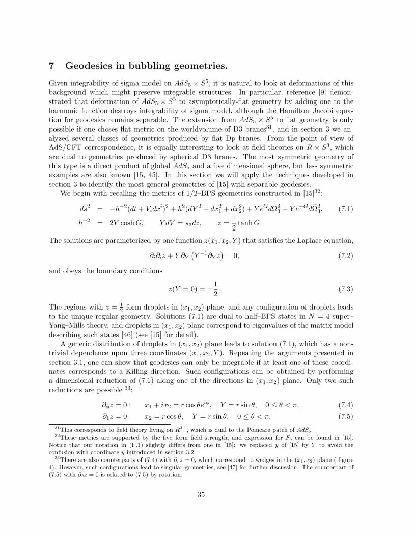
7 Geodesics in bubbling geometries.
Given integrability of sigma model on AdS5 × S5, it is natural to look at deformations of thisbackground which might preserve integrable structures. In particular, reference [9] demon-strated that deformation of AdS5 × S5 to asymptotically-flat geometry by adding one to theharmonic function destroys integrability of sigma model, although the Hamilton–Jacobi equa-tion for geodesics remains separable. The extension from AdS5 × S5 to flat geometry is onlypossible if one choses flat metric on the worldvolume of D3 branes31, and in section 3 we an-alyzed several classes of geometries produced by flat Dp branes. From the point of view ofAdS/CFT correspondence, it is equally interesting to look at field theories on R × S3, whichare dual to geometries produced by spherical D3 branes. The most symmetric geometry ofthis type is a direct product of global AdS5 and a five dimensional sphere, but less symmetricexamples are also known [15, 45]. In this section we will apply the techniques developed insection 3 to identify the most general geometries of [15] with separable geodesics.
We begin with recalling the metrics of 1/2–BPS geometries constructed in [15]32:
ds2 = −h−2(dt+ Vidxi)2 + h2(dY 2 + dx21 + dx22) + Y eGdΩ2
3 + Y e−GdΩ23, (7.1)
h−2 = 2Y coshG, Y dV = ⋆3dz, z =1
2tanhG
The solutions are parameterized by one function z(x1, x2, Y ) that satisfies the Laplace equation,
∂i∂iz + Y ∂Y(
Y −1∂Y z)
= 0, (7.2)
and obeys the boundary conditions
z(Y = 0) = ±1
2. (7.3)
The regions with z = 12 form droplets in (x1, x2) plane, and any configuration of droplets leads
to the unique regular geometry. Solutions (7.1) are dual to half–BPS states in N = 4 super–Yang–Mills theory, and droplets in (x1, x2) plane correspond to eigenvalues of the matrix modeldescribing such states [46] (see [15] for detail).
A generic distribution of droplets in (x1, x2) plane leads to solution (7.1), which has a non-trivial dependence upon three coordinates (x1, x2, Y ). Repeating the arguments presented insection 3.1, one can show that geodesics can only be integrable if at least one of these coordi-nates corresponds to a Killing direction. Such configurations can be obtained by performinga dimensional reduction of (7.1) along one of the directions in (x1, x2) plane. Only two suchreductions are possible 33:
∂φz = 0 : x1 + ix2 = r cos θeiφ, Y = r sin θ, 0 ≤ θ < π, (7.4)
∂1z = 0 : x2 = r cos θ, Y = r sin θ, 0 ≤ θ < π. (7.5)
31This corresponds to field theory living on R3,1, which is dual to the Poincare patch of AdS5
32These metrics are supported by the five–form field strength, and expression for F5 can be found in [15].Notice that our notation in (F.1) slightly differs from one in [15]: we replaced y of [15] by Y to avoid theconfusion with coordinate y introduced in section 3.2.
33There are also counterparts of (7.4) with ∂rz = 0, which correspond to wedges in the (x1, x2) plane ( figure4). However, such configurations lead to singular geometries, see [47] for further discussion. The counterpart of(7.5) with ∂2z = 0 is related to (7.5) by rotation.
35
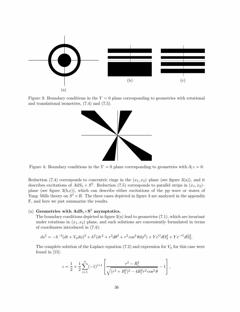
(a)
(b) (c)
Figure 3: Boundary conditions in the Y = 0 plane corresponding to geometries with rotationaland translational isometries, (7.4) and (7.5).
Figure 4: Boundary conditions in the Y = 0 plane corresponding to geometries with ∂rz = 0.
Reduction (7.4) corresponds to concentric rings in the (x1, x2)–plane (see figure 3(a)), and itdescribes excitations of AdS5 × S5. Reduction (7.5) corresponds to parallel strips in (x1, x2)–plane (see figure 3(b,c)), which can describe either excitations of the pp–wave or states ofYang–Mills theory on S1×R. The three cases depicted in figure 3 are analyzed in the appendixF, and here we just summarize the results.
(a) Geometries with AdS5×S5 asymptotics.The boundary conditions depicted in figure 3(a) lead to geometries (7.1), which are invariantunder rotations in (x1, x2) plane, and such solutions are conveniently formulated in termsof coordinates introduced in (7.4):
ds2 = −h−2(dt+ Vφdφ)2 + h2(dr2 + r2dθ2 + r2 cos2 θdφ2) + Y eGdΩ2
3 + Y e−GdΩ23.
The complete solution of the Laplace equation (7.2) and expression for Vφ for this case werefound in [15]:
z =1
2+
1
2
n∑
i=1
(−1)i+1
r2 −R2i
√
(r2 +R2i )
2 − 4R2i r
2 cos2 θ− 1
,
36
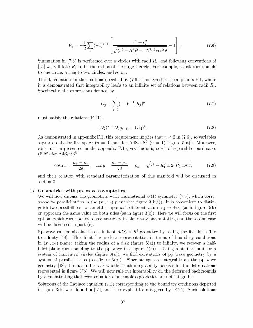
Vφ = −1
2
n∑
i=1
(−1)i+1
r2 + r2i√
(r2 +R2i )
2 − 4R2i r
2 cos2 θ− 1
, (7.6)
Summation in (7.6) is performed over n circles with radii Ri, and following conventions of[15] we will take R1 to be the radius of the largest circle. For example, a disk correspondsto one circle, a ring to two circles, and so on.
The HJ equation for the solutions specified by (7.6) is analyzed in the appendix F.1, whereit is demonstrated that integrability leads to an infinite set of relations between radii Ri.Specifically, the expressions defined by
Dp ≡n∑
j=1
(−1)j+1(Rj)p (7.7)
must satisfy the relations (F.11):
(D2)k−1D2(k+1) = (D4)
k. (7.8)
As demonstrated in appendix F.1, this requirement implies that n < 2 in (7.6), so variablesseparate only for flat space (n = 0) and for AdS5×S5 (n = 1) (figure 5(a)). Moreover,construction presented in the appendix F.1 gives the unique set of separable coordinates(F.22) for AdS5×S5
cosh x =ρ+ + ρ−
2d, cos y =
ρ+ − ρ−2d
, ρ± =√
r2 +R21 ± 2rR1 cos θ, (7.9)
and their relation with standard parameterization of this manifold will be discussed insection 8.
(b) Geometries with pp–wave asymptoticsWe will now discuss the geometries with translational U(1) symmetry (7.5), which corre-spond to parallel strips in the (x1, x2) plane (see figure 3(b,c)). It is convenient to distin-guish two possibilities: z can either approach different values x2 → ±∞ (as in figure 3(b)or approach the same value on both sides (as in figure 3(c)). Here we will focus on the firstoption, which corresponds to geometries with plane wave asymptotics, and the second casewill be discussed in part (c).
Pp–wave can be obtained as a limit of AdS5 × S5 geometry by taking the five–form fluxto infinity [48]. This limit has a clear representation in terms of boundary conditionsin (x1, x2) plane: taking the radius of a disk (figure 5(a)) to infinity, we recover a half-filled plane corresponding to the pp–wave (see figure 5(c)). Taking a similar limit for asystem of concentric circles (figure 3(a)), we find excitations of pp–wave geometry by asystem of parallel strips (see figure 3(b)). Since strings are integrable on the pp–wavegeometry [48], it is natural to ask whether such integrability persists for the deformationsrepresented in figure 3(b). We will now rule out integrability on the deformed backgroundsby demonstrating that even equations for massless geodesics are not integrable.
Solutions of the Laplace equation (7.2) corresponding to the boundary conditions depictedin figure 3(b) were found in [15], and their explicit form is given by (F.24). Such solutions
37
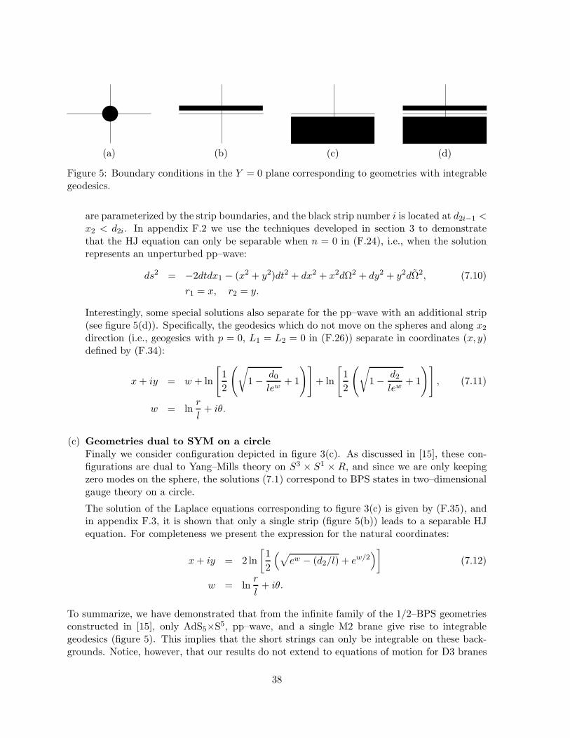
(a) (b) (c) (d)
Figure 5: Boundary conditions in the Y = 0 plane corresponding to geometries with integrablegeodesics.
are parameterized by the strip boundaries, and the black strip number i is located at d2i−1 <x2 < d2i. In appendix F.2 we use the techniques developed in section 3 to demonstratethat the HJ equation can only be separable when n = 0 in (F.24), i.e., when the solutionrepresents an unperturbed pp–wave:
ds2 = −2dtdx1 − (x2 + y2)dt2 + dx2 + x2dΩ2 + dy2 + y2dΩ2, (7.10)
r1 = x, r2 = y.
Interestingly, some special solutions also separate for the pp–wave with an additional strip(see figure 5(d)). Specifically, the geodesics which do not move on the spheres and along x2direction (i.e., geogesics with p = 0, L1 = L2 = 0 in (F.26)) separate in coordinates (x, y)defined by (F.34):
x+ iy = w + ln
[
1
2
(
√
1− d0lew
+ 1
)]
+ ln
[
1
2
(
√
1− d2lew
+ 1
)]
, (7.11)
w = lnr
l+ iθ.
(c) Geometries dual to SYM on a circleFinally we consider configuration depicted in figure 3(c). As discussed in [15], these con-figurations are dual to Yang–Mills theory on S3 × S1 × R, and since we are only keepingzero modes on the sphere, the solutions (7.1) correspond to BPS states in two–dimensionalgauge theory on a circle.
The solution of the Laplace equations corresponding to figure 3(c) is given by (F.35), andin appendix F.3, it is shown that only a single strip (figure 5(b)) leads to a separable HJequation. For completeness we present the expression for the natural coordinates:
x+ iy = 2 ln
[
1
2
(
√
ew − (d2/l) + ew/2)
]
(7.12)
w = lnr
l+ iθ.
To summarize, we have demonstrated that from the infinite family of the 1/2–BPS geometriesconstructed in [15], only AdS5×S5, pp–wave, and a single M2 brane give rise to integrablegeodesics (figure 5). This implies that the short strings can only be integrable on these back-grounds. Notice, however, that our results do not extend to equations of motion for D3 branes
38
(which are expected to be integrable, as least for 1/2–BPS objects) since the HJ equation (1.3)did not take into account coupling to the RR field. We also found that the separable coordinates(x, y) given by (7.9) are the same elliptic coordinates (or their limits) as the one encountered insection 3.2, and in the next section we will discuss the relation between (x, y) and the standardparameterization of AdS5×S5.
8 Elliptic coordinates and standard parameterization of AdSp×Sq
In the last section we have demonstrated that the HJ equation for geodesics on 1/2–BPS geome-tries of [15] separates only for AdS5×S5 and for its pp–wave limit. Moreover, this separationhappens in the elliptic coordinates (7.9). On the other hand, equations for supergravity fieldson AdS5×S5 are usually analyzed in the standard parameterization34:
ds2 = L2[
− cosh2 ρdt2 + dρ2 + sinh2 ρdΩ23 + dχ2 + cos2 χdφ2 + sin2 χdΩ2
]
(8.1)
and the detailed study of [49] uses the explicit SO(4, 2) × SO(6) symmetry of this metricto separate the resulting equations and to find the mass spectrum of supergravity modes onAdS5×S5. This suggests a close relation between the elliptic coordinates and (8.1), which will beclarified in this subsection. We will also discuss the elliptic coordinates for AdS7×S4, AdS4×S7,and AdS3×S3.
Standard parameterization of AdS5×S5.To relate the standard parameterization (8.1) with elliptic coordinates (7.9), we first recall
the map between (8.1) and variables used in (7.1) (see [15]):
x1 + ix2 = L2 cosh ρ cosχeiφ, Y = L2 sinh ρ sinχ, φ = φ− t. (8.2)
Comparing this with (7.4), we relate the standard coordinates (8.1) with (r, θ),
L2 sinh ρ sinχ = r sin θ, L2 cosh ρ cosχ = r cos θ, (8.3)
and substitution into (7.9) gives
ρ± = R1 [cosh ρ± cosχ] ⇒ x = ρ, y = χ. (8.4)
We conclude that the standard coordinates (8.1) on AdS5×S5 can be viewed as elliptic coordi-nates on the base of the LLM geometries (7.1) in IIB supergravity.
1/2–BPS geometries in M-theory.Let us now turn to the LLM geometries in M-theory [15]:
ds211 = −4e2λ(1 + Y 2e−6λ)(dt+ Vidxi)2 +
e−4λ
1 + Y 2e−6λ
[
dY 2 + eD(dx21 + dx22)]
+ 4e2λdΩ25 + Y 2e−4λdΩ2
2
e−6λ =∂YD
Y (1− Y ∂YD), Vi =
1
2ǫij∂jD.
34We denoted an azimuthal direction on S5 by χ to avoid confusion with coordinate θ introduced in (7.4).
39
Metric (8.5) is parameterized by one function D satisfying the Toda equation,
(∂21 + ∂22)D + ∂2Y eD = 0, (8.5)
on a three–dimensional base,
ds2base = dY 2 + eD[
dx21 + dx22]
, (8.6)
and some known boundary conditions in the Y = 0 plane. Although (8.5) is much more com-plicated than the Laplace equation (7.2), we expect that repetition of the arguments presentedin section 7 ensures that function D can only depend on two rather than three variables, andin this case (8.5) can be rewritten as a Laplace equation via a nonlocal change of variables [50].Specifically, for the rotationally–invariant case, it is convenient to rewrite the metric on thebase as35
ds2base = dY 2 + eD[
dR2 +R2dφ2]
= dY 2 + eD[
dX2 + dφ2]
(8.7)
Function D = D + 2 lnR defined above satisfied the same Toda equation (8.5) as D, and interms of (X,Y ) this equation can be rewritten as
∂2XD + ∂2Y eD = 0 (8.8)
The Toda equation with translational invariance along x1 can also be written as (8.7)–(8.8)after a replacement (x1, x2,D) → (φ,X, D). A nonlocal change of coordinates [50, 15],
eD = ζ2, Y = ζ∂ζV, X = ∂ηV, (8.9)
maps the nonlinear Toda equation (8.8) into the Laplace equation for function V :
ζ−1∂ζ(ζ∂ζV ) + ∂2ηV = 0. (8.10)
Unfortunately, the boundary conditions for V are rather complicated [15] (see [51] for a detaileddiscussion), and simple expressions for D and Vφ similar to (7.6) are not known. Nevertheless,the results presented in sections 6 and 7 strongly suggest that the HJ equation on the geometries(8.5) would only separate on the most symmetric backgrounds: AdS7×S4, AdS4×S7, and the ppwave. Let us discuss the relation between the standard parameterizations of these backgroundsand the elliptic coordinates.
Since elliptic coordinates are only defined in flat space, we begin with rewriting the (X,Y )sector of (8.7) in a conformally–flat form. It turns out that this is accomplished by going tocoordinates (ξ, η) defined by (8.9), and metric (8.7) becomes
ds2base = ζ2[
(∂ζ∂ηV )2 + (∂2ηV )2] (
dζ2 + dη2)
+ dφ2
(8.11)
After introducing the standard polar parameterization (r, θ),
ζ = r sin θ, η = r cos θ, (8.12)
35We introduced an obvious notation: x1 + ix2 = Reiφ, X = lnR.
40
one can define the elliptic coordinates by (3.55). We will now compare these coordinates withthe standard parameterization of AdS7×S4 and AdS4×S7.
Standard parameterization of AdS7×S4.Solution corresponding to AdS7×S4,
ds2 = 4L2[
dρ2 + sinh2 ρdΩ25 − cosh2 ρdt2
]
+ L2[
dχ2 + sin2 χdΩ22 + cos2 χdφ2
]
, (8.13)
is given by equation (3.15) in [15] with a replacement r → 2 sinh ρ:
x1 + ix2 = cosh2 ρ cosχeiφ, Y =1
L3sinh2 ρ sinχ, eD =
1
L6tanh2 ρ. (8.14)
Substitution into (8.9) gives the expression for ζ and equations for V :
ζ =1
2L3sinh(2ρ) cos χ, ∂ζV = tanh ρ tanχ, ∂ηV = ln
[
cosh2 ρ cosχ]
. (8.15)
Coordinate η can be determined using the relation dη = ⋆2dζ (recall (8.11) and (ρ, χ) sector of(8.13)):
η =1
2L3cosh(2ρ) sinχ. (8.16)
For completeness we also write the expression for V , which comes from integrating the differ-ential equations in (8.15), although it will not play any role in our discussion:
V =1
2L3sinχ
[
cosh(2ρ) ln(cosχ cosh2 ρ)− 1]
+1
2L3ln
[
tanχ+ π
2
2
]
.
To deduce the elliptic coordinates, we begin with finding the counterpart of equations (8.3)by rewriting the left–hand sides of (8.12) in terms of (ρ, χ):
1
2L3sinh(2ρ) cos χ = r sin θ,
1
2L3cosh(2ρ) sin χ = r cos θ. (8.17)
Substitution of these relations into the definition (3.55) with R1 = 1/(2L3), leads to identifica-tion of the elliptic coordinates (x, y) with (ρ, χ) (compare with equation (8.4)):
x = 2ρ, y =π
2− χ. (8.18)
This implies that the standard parameterization of AdS7×S4 has a simple geometrical meaning:coordinates (ρ, χ) coincide with elliptic coordinates on the two–dimensional space spanned by(η, ζ).
Standard parameterization of AdS4×S7.Solution corresponding to AdS4×S7,
ds2 = L2[
dρ2 + sinh2 ρdΩ22 − cosh2 ρdt2
]
+ 4L2[
dχ2 + sin2 χdΩ25 + cos2 χdφ2
]
,
41
is given by equation (3.16) in [15] with a replacement r → 2 sinh ρ:
x1 + ix2 =√
cosh ρ cosχeiφ, Y =1
L3sinh ρ sin2 χ, eD =
4
L6cosh ρ sin2 χ. (8.19)
Substitution into (8.9) gives the expression for ζ and η:
ζ =1
L3cosh ρ sin(2χ), η = − 1
L3sinh ρ cos(2χ). (8.20)
For completeness we also give the equations for V and their solution:
∂ζV =1
2tanh ρ tanχ, ∂ηV = ln
[
√
cosh ρ cosχ]
V =1
2L3
[
sinh ρ− 2 arctan[
tanhρ
2
]
− 2 cos(2χ) sinh ρ ln[
√
cosh ρ cosχ]]
.
Combining (8.20), and analog of (8.12)36,
ζ = r cos θ, η = −r sin θ. (8.21)
and (3.55) with R1 = 1/(L3), we identify the elliptic coordinates (x, y) with (ρ, χ) (comparewith equations (8.4) and (8.18)):
x = ρ, y =π
2− 2χ. (8.22)
Standard parameterization of AdS3×S3.As our final example of elliptic coordinates, we consider AdS3×S3 in global parameterization,
which can be obtained by taking the near horizon limit (H → Q/f) in (6.18) [52]:
ds2 = Q
[
−((r′)2 + a2)dt2
Q2+
(dr′)2
(r′)2 + a2+
(r′du)2
Q2+ (dθ′)2 + sin2 θ′dφ2 + cos2 θ′dψ2
]
,
φ = φ+a
Qt, ψ = ψ +
a
Qu. (8.23)
Rewriting the metric in terms of the elliptic coordinates defined by (6.21):
ds2 = Q
[
− cosh2 x(adt)2
Q2+ dx2 + sinh2 x
(adu)2
Q2+ dy2 + sin2 ydφ2 + cos2 ydψ2
]
,
(8.24)
we conclude that these coordinates give the standard parameterization of AdS3×S3.
Pp–wave limits of AdSp×Sq.We conclude this section by commenting on the pp–wave limits of AdSp×Sq.The pp–wave limit of AdS5×S5,
ds2 = −2dtdx1 − (r21 + r22)dt2 + dr21 + r21dΩ
2 + dr22 + r22dΩ2, (8.25)
36We redefined angle θ in (8.12). Alternatively, one can keep (8.12) and shift θ in (3.55).
42
is obtained by taking
z =1
2
x2√
x22 + Y 2, V =
1
2
1√
x22 + Y 2dx1 (8.26)
in (7.1) and setting
Y = r1r2, x2 =1
2(r21 − r22). (8.27)
This leads to a very simple relation for the polar coordinates defined by (7.5)
r1 =√2r cos
θ
2, r2 =
√2r sin
θ
2. (8.28)
Equation for geodesics in the geometry (8.25) separates in variables (r1, r2), which can beobtained from the elliptic coordinates (8.3)–(8.4) by taking the pp–wave limit:
L→ ∞, fixed r1 = Lx, r2 = Ly. (8.29)
We conclude that in the pp–wave limit, the elliptic coordinate degenerate into the radii of thethree–spheres.
The pp–wave limit of AdSp×Sq in M theory,
ds2 = −2dtdx1 − (r22 + r25)dt2 + dr22 + r22dΩ
22 + dr25 + r25dΩ
25 (8.30)
is given by equation (3.14) of [15]:
Y =r25r24, x2 =
r254
− r222, eD =
r254
(8.31)
This translates into
ζ =r52, η =
r22, V =
r2r25
8− r32
12= ζ2η − 2
3η3 (8.32)
via (8.9)37. These expressions can be obtained from (8.15)–(8.16) or from (8.20) by taking thelarge–L limits, and in both cases we arrive at a counterpart of (8.29):
L → ∞, fixed r2 = Lx, r5 = L(π
2− y)
. (8.33)
As in the case of the type IIB pp–waves, we conclude that the elliptic coordinates degenerateinto the radii of the spheres.
The pp–wave limit of the AdS3×S3 geometry (8.24) is obtained by writing
y =y√Q, x =
x√Q, u =
Qu
a, t =
Q
2a
(
x+ +x−
Q
)
, ψ =1
2
(
x+ − x−
Q
)
(8.34)
37Since we are dealing with translational rather than rotational symmetry, D = D and X = x2 in (8.9)
43
and sending Q to infinity, while keeping all hatted variables fixed. This results in the metric
ds2 = −dx+dx− − 1
4(x2 + y2)(dx+)2 + dx2 + x2du2 + dy2 + y2dφ2.
Once again, elliptic coordinates degenerate to the radii of the one–spheres.
To summarize, we have demonstrated that in all examples of AdSp×Sq, where the HJequation separates between the sphere and AdS in global coordinates, such separation emergesas a particular case of integrability in elliptic coordinates, and standard parameterization ofAdSp×Sq coincides with elliptic coordinates on the relevant flat base. In the pp–wave limits ofAdSp×Sq, the elliptic coordinates reduce to the radii of the appropriate spheres.
9 Discussion
Integrability of geodesics and Klein–Gordon equation has led to numerous insights into physicsof black holes. While the black hole solutions are few and far between, the large classes ofsupersymmetric geometries are known, and in this article we have classified such solutions withintegrable geodesics. This integrability is demonstrated to imply that the HJ equation mustseparate in the elliptic coordinates. For branes with flat worldvolumes, such separation, thatextends the known result for the spherical coordinates, can only occur for special distributionsof sources, which are analyzed in section 3. For the curved supersymmetric branes, the ellipticcoordinates can only be introduced in the most symmetric cases, and as demonstrated in section7, all these situations reduce to AdSp×Sq or their pp–wave limits.
Our results rule out integrability of N=4 SYM beyond the large N limit. Specifically, weproved that the excitations of strings around heavy supersymmetric states (∆ ∼ N2) are notintegrable. While this is consistent with general expectations, it is somewhat surprising thatnone of the 1/2–BPS geometries give rise to integrable sectors. It would be interesting to extendthis result to states with fewer supersymmetries.
Our results also have unfortunate consequences for the technical progress in the fuzzballprogram. While a large number of geometries corresponding to microscopic states of black holeshave been constructed in the last decade, the detailed calculations of the absorption/emissionrates have only been performed for the simplest cases. Such calculations are based on solvingthe Klein–Gordon equation, and as we demonstrated in section 6, this equation, as well as theHamilton–Jacobi equation for geodesics, cannot separate beyond the known cases. Our resultsdo not imply that a study of geodesics on a particular background is hopeless. A lot of usefulinformation can be extracted by performing numerical integration of the equations of motionand by studying some special configurations rather than generic geodesics.
Acknowledgements
We thank Hai Lin and Filip Petrescu for useful discussions. This work is supported in part byNSF grant PHY-1316184.
44
A Examples of separable Hamilton–Jacobi equations
In this appendix we provide some technical details pertaining to derivation of the results pre-sented in sections 2 and 3. In particular, we write down the explicit expressions for SL onthe sphere (A.7), the complete integral for R in the elliptic coordinates (A.16) and make theconnection between the holomorphic function introduced in (3.45) and the standard ellipticcoordinates (2.12).
A.1 Motion on a sphere
While discussing separation of variables in the Hamilton–Jacobi equation, on several occasionswe have encountered equation
hij∂S
(k)Lk
∂yi∂S
(k)Lk
∂yj= L2
k, (A.1)
on a k–dimensional sphere Sk (see, for example, (2.7), (3.25)). In this appendix we will writethe complete integral of (3.25) using induction.
Writing the metric on Sk as
hijdyidyj = dy2k + sin2 ykdΩ
2k−1, (A.2)
and splitting S(k)L as
S(k)Lk
(y1, . . . , yk) = Fk(yk) + S(k−1)Lk−1
(y1, . . . , yk−1), (A.3)
we can rewrite equation (A.1) as
(F ′k)
2 +L2k−1
sin2 yk= L2
k, (A.4)
hij∂S
(k−1)Lk−1
∂yi
∂S(k−1)Lk−1
∂yj= L2
k−1, (A.5)
Solving the first equation38,
Fk =
∫
dyksin yk
√
L2k sin
2 yk − L2k−1, (A.6)
and applying induction, we arrive at the complete integral of (A.1) that depends on k parametersLj:
S(k)Lk
(y1, . . . , yk) =
k∑
j=2
∫
dyjsin yj
√
L2j sin
2 yk − L2j−1 + L1y1. (A.7)
This explicit solution should be substituted into (2.5).
38Although the integral in (A.6) can be performed, the result is not very illuminating.
45
A.2 Two–center potential and elliptic coordinates
In section 2 we reviewed separation of variables in elliptic coordinates, and here we presentsome details of that construction.
The motion of a particle in the geometry produced by two stacks of Dp branes is governedby the Hamilton–Jacobi equation (2.11)
(∂rR)2 +
1
r2(∂θR)
2 +L2
r2 sin2 θ+Hpµp
µ = 0, (A.8)
where H is given by (2.9)
H = a+Q
ρ6−p+
+Q
ρ6−p−
, ρ± =√
r2 + d2 ± 2rd cos θ (A.9)
To rewrite (A.8) in terms the elliptic coordinates (ξ, η) defined by (2.12), we notice that (A.8)can be viewed as a Hamilton–Jacobi equation corresponding to an effective Lagrangian for rand θ:
Leff = r2 + r2θ2 − L2
r2 sin2 θ−Hpµp
µ. (A.10)
Rewriting the last expression in terms of ξ, η,
Leff = d2(ξ2 − η2)
[
ξ2
ξ2 − 1+
η2
1− η2
]
− L2
d2(ξ2 − 1)(1 − η2)−Hpµp
µ (A.11)
and going back to the Hamilton–Jacobi equation for S(ξ, η), we find
1
d2(ξ2 − η2)
[
(ξ2 − 1)(∂ξR)2 + (1− η2)(∂ηR)
2 +
(
1
ξ2 − 1+
1
1− η2
)
L2
]
+Hpµpµ = 0.
(A.12)
This equation separates in variables (ξ, η) is and only if
(ξ2 − η2)H = U1(ξ) + U2(η). (A.13)
Rewriting the harmonic function (A.9) in terms of elliptic coordinates, we find that the lefthand side of the last expression,
(ξ2 − η2)H = (ξ2 − η2)
[
a+Q
[d(ξ + η)]6−p+
Q
[d(ξ − η)]6−p
]
, (A.14)
separates only for p = 5. In this case equation (A.12) becomes
[
(ξ2 − 1)(∂ξR)2 +
L2
ξ2 − 1+ pµp
µ(aξ2 + 2Qξ)
]
+
[
(1− η2)(∂ηR)2 +
L2
1− η2− pµp
µaη2]
= 0, (A.15)
46
and its complete integral is
R =
∫
dξ√
ξ2 − 1
[
−λ− L2
ξ2 − 1+M2(aξ2 + 2Qξ)
]1/2
+
∫
dη√
1− η2
[
λ− L2
1− η2−M2aη2
]1/2
(A.16)
Here λ is a separation constant and M2 = −pµpµ.To embed the elliptic coordinates in the general framework presented in section 3.2, we have
to find the holomorphic function h(w) defined by (3.45). Comparing the kinetic terms in (A.12)with equation (3.38), we find the relation
1
d2(ξ2 − η2)
[
(ξ2 − 1)(∂ξR)2 + (1− η2)(∂ηR)
2]
=1
A(x, y)
[
(∂xR)2 + (∂yR)
2]
,
which leads to expressions for (ξ, η) in terms of (x, y):
ξ = coshx, η = cos y. (A.17)
The relation between coordinates (r, θ) and (x, y) looks rather complicated (see (2.12)),
cosh x = ξ ≡ ρ+ + ρ−2d
, cos y = η ≡ ρ+ − ρ−2d
(A.18)
ρ± =√
r2 + d2 ± 2rd cos θ, (A.19)
but it can be simplified by making use of the complex variables (3.42).First we rewrite equations (A.18) as an expression for z in terms of ξ and η:
ex = ξ +√
ξ2 − 1, eiy = η + i√
1− η2
z = x+ iy = ln[
(ξ +√
ξ2 − 1)(η + i√
1− η2)]
(A.20)
Next we recall the definition (3.42) of the complex variable w and use (A.19) to write ρ± interms of it:
ρ+ =√
(r + deiθ)(r + de−iθ) = d
√
(
l
dew + 1
)(
l
dew + 1
)
, ρ− = d
√
(
l
dew − 1
)(
l
dew − 1
)
.
To simplify the expressions for various ingredients appearing in (A.20) it is convenient to defineholomorphic functions W±:
W+ ≡√
l
dew + 1, W− ≡
√
l
dew − 1. (A.21)
Then we find
ξ =W+W+ +W−W−
2, η =
W+W+ −W−W−
2.
√
ξ2 − 1 =W−W+ +W+W−
2,
√
1− η2 =W−W+ −W+W−
2i.
47
Substitution of these results into (A.20) leads to the desired relation between z and w:
z = ln
[
1
4(W+ +W−)
2((W+)2 − (W−)
2)
]
= ln
[
l
dew +
√
l2
d2e2w − 1
]
(A.22)
Finally, the asymptotic behavior (3.49) determines l in terms of d: l = d/2.As expected from the discussion in section 3.2, z turns out to be a holomorphic function:
z = h(w) = ln
[
1
2
ew +√
e2w − 4
]
. (A.23)
Finally, by comparing (A.15) with (3.38), (3.39), we extract the expressions for the potentialsU1(x) and U2(y):
U1(x) =L2
sinh2 x−M2(a cosh2 x+ 2Q cosh x)
U2(y) =L2
sin2 y+M2a cos2 y. (A.24)
To summarize, in this section we demonstrated that the HJ equation (A.8) with H given by(A.9) separates in the elliptic coordinates (2.12), (A.20), and the relevant potentials are givenby (A.24). We also embedded the elliptic coordinates into the general discussion presented insection 3.2 by deriving equation (A.23).
B Ellipsoidal coordinates
As demonstrated in section 3.1, if the HJ equation (3.10) separates for k > 2, such separationmust occur in ellipsoidal coordinates, including degenerate cases. In this appendix we willdemonstrate that a combination of the Laplace equation (3.6) and the requirement (3.5) rulesout such separation. To avoid unnecessary complications, we will first give the detailed discus-sion of the k = 3 case, and in section B.2 we will comment on minor changes which emergefrom generalization to k > 3.
B.1 Ellipsoidal coordinates for k = 3
The ellipsoidal coordinates have been introduced by Jacobi [30], and there are several equivalentdefinitions. We will follow the notation of [53].
Ellipsoidal coordinates, (x1, x2, x3) are defined as three solutions of a cubic equation for x:
r21x+ a2
+r22
x+ b2+
r23x+ c2
= 1, (B.1)
where a > b > c > 0 and r1, r2, r3 correspond to our rk from (3.4). The roots are arranged inthe following order:
x1 ≥ −c2 ≥ x2 ≥ −b2 ≥ x3 ≥ −a2 (B.2)
48
Coordinates (r1, r2, r3) can be expressed through (x1, x2, x3) by39
r1 = ±[
(x1 + a2)(x2 + a2)(x3 + a2)
(b2 − a2)(c2 − a2)
]1/2
, r2 = ±[
(x1 + b2)(x2 + b2)(x3 + b2)
(c2 − b2)(a2 − b2)
]1/2
,
r3 = ±[
(x1 + c2)(x2 + c2)(x3 + c2)
(a2 − c2)(b2 − c2)
]1/2
.
In terms of the elliptic coordinates, the metric of the flat three dimensional space becomes
ds2 = dx21 + dr22 + dr23 = h21dx21 + h22dx
22 + h23dx
23, (B.3)
h21 =(x1 − x2)(x1 − x3)
4R1, R1 = (x1 + a2)(x1 + b2)(x1 + c2)
Expressions for h2, h3, R2, R3 are obtained by making a cyclic permutation of indices. Tosimplify the formulas appearing below, it is convenient to introduce dij ≡ xi − xj .
In ellipsoidal coordinates equation (3.10) becomes
4
d12d13d23
[
d23R1(∂1S)2 + d31R2(∂2S)
2 + d12R3(∂3S)2]
+3∑
j=1
L2j
r2j+Hpµp
µ = 0. (B.4)
Before imposing the Laplace equation (3.6) we will demonstrate that separation requires thatd1 = d2 = d3 = 0 in (3.4). Indeed, the separation implies that
S(x1, x2, x3) = S1(x1) + S2(x2) + S3(x3). (B.5)
Then multiplying equation (B.4) by d12d13d23 and applying ∂21∂22 to the result, we find a relation
which does not involve S:
∂21∂22
d12d13d23
3∑
j=1
L2j
r2j+Hpµp
µ
= 0. (B.6)
Let us assume that d1 > 0 in (3.4), then the last relation must hold for all values of L1, thus
∂21∂22
[
d12d13d23r21
]
= ∂21∂22
[
(b2 − a2)(c2 − a2)d12d13d23(x1 + a2)(x2 + a2)(x3 + a2)
]
= 0. (B.7)
This condition can only be satisfied if a = b, this degenerate case corresponds to oblatespheroidal coordinates:
r1 + ir2 =
[
(x1 + a2)(x2 + a2)
a2 − c2
]1/2
eiφ, r3 = ±[
(x1 + c2)(x2 + c2)
c2 − a2
]1/2
(B.8)
We will now demonstrate that separation of the HJ equation in spheroidal coordinates impliesthat ∂φH = 0, i.e., violation of (3.5) for i = 1, j = 2. This will falsify our assumption d1 > 0,and similar arguments will show that separability of the HJ equation requires d2 = d3 = 0.
39We recall that rj must be non-negative if dj > 0 in (3.4), otherwise rj varies from minus infinity to infinity.
49
To simplify notation and to connect to our discussion in section 3.2 it is convenient to usean alternative form of the oblate spheroidal coordinates (B.8):
x1 = (a2 − c2) cosh2 x− a2, x2 = (a2 − c2) cos2 y − a2 (B.9)
This gives expressions for the radii:
r1 + ir2 = A coshx cos yeiφ, r3 = ±A sinhx sin y, A =√
a2 − c2, (B.10)
and the metric becomes
ds2 = A2(sinh2 x+ sin2 y)(dx2 + dy2) +A2 cosh2 x cos2 ydφ2 (B.11)
Notice that these are precisely the elliptic coordinates found in section 3.2. The HJ equation(3.10) in coordinates (x, y) has the form
(∂xS)2 + (∂yS)
2
A2(sinh2 x+ sin2 y)+
1
A2 cosh2 x cos2 y(∂φS)
2 +3∑
j
L2j
r2j+Hpµp
µ = 0, (B.12)
and it does not separate unless
H cosh2 x cos2 y = X(x, y) + Φ(φ) (B.13)
Recalling that at large values of x function H does not depend on φ (see (3.7)), we concludethat Φ′(φ) = 0, then ∂φH = 0 everywhere. As already mentioned, this relation violates thecondition (3.5), so our assumption d1 > 0 was false. Repeating this arguments for the remainingtwo spheres, we conclude that d1 = d2 = d3 = 0 in (3.4) and (3.6).
We will now combine the integrability condition (B.6),
∂2i ∂2j [d12d13d23H] = 0, (B.14)
with Laplace equation (3.6) to rule out separability of the HJ equation in ellipsoidal coordinates,
4
d12d13d23
[
R1d23(∂1S)2 + d31R2(∂2S)
2 + d12R3(∂3S)2]
+Hpµpµ = 0. (B.15)
Since we have already established that d1 = d2 = d3 = 0, equation (3.6) reduces to the Laplaceequation on a flat three–dimensional space formed by (r1, r2, r3), and it can be rewritten interms of ellipsoidal coordinates using (B.3):
4
d12d31d23
[
d23√
R1∂1(√
R1∂1H) + d31√
R2∂2(√
R2∂2H) + d12√
R3∂3(√
R3∂3H)]
= 0.
(B.16)
In the remaining part of this subsection we will demonstrate that equations (B.14), (B.16),(3.5), (3.7) are inconsistent with separability of (B.15).
Let us assume that the HJ equation (B.15) separates. Although the ellipsoidal coordinatesare restricted by (B.2) the formal separation (B.5) must persist beyond this range. In particular,
50
it is convenient to look at the limit x1 → x2, where x2 is kept as a free parameter. The Laplaceequation (B.16) guarantees that H remains finite in this limit, then equation (B.15) reduces to
[
R1(S′1)
2 −R2(S′2)
2]
x1=x2= 0 (B.17)
This implies that
S1(x1) = F (x1), S2(x2) = F (x2) (B.18)
with the same function F . Repeating this argument for x1 = x3, we conclude that
S3(x3) = F (x3). (B.19)
Rewriting (B.15) in terms of F , we conclude that H must be symmetric under interchange ofits arguments40, and combination of this symmetry with integrability conditions (B.14) leadsto severe restrictions on the form of H.
Taking (i, j) = (1, 2) in (B.14), and solving the resulting equation, we find
H =1
d12d13d23[G1(x1, x3)x2 +G2(x2, x3)x1 +G01(x1, x3) +G02(x2, x3)] , (B.20)
where G1, G2, G01, G02 are some undetermined functions of their arguments. Applying (B.14)with different values of (i, j), we find further restrictions on the form of H:
H =1
d12d13d23
∑
i 6=j
Gij(xi)xj +∑
i
G0i(xi)
(B.21)
Symmetry of H under interchange of any pair of coordinates implies that G0i = 0, matrix Gijis anti-symmetric, and all Gij can be reduced to a single function41 G:
H =1
d12d13d23[G(x1)(x2 − x3) +G(x2)(x3 − x1) +G(x3)(x1 − x2)]
=G(x1)
d12d13+G(x2)
d21d23+G(x3)
d31d32. (B.22)
Notice that constant and linear functions G lead to H = 0, and quadratic G gives constant H.Substitution of (B.22) into (B.16) leads to a complicated equation for function G:
R1d23d12d13
G′′1 − 2
d23d212d
213
(d12 + d13)R1G′1 +
d232d12d13
R′1G
′1
+d23
d212d213
[
3(R1 −R0)− (x1x2 + x1x3 + x2x3)R′′
0
2−R′
0(x1 + x2 + x3)− 3x1x2x3
]
G1
+perm = 0 (B.23)
Here we used a shorthand notation: R0 = R(0), R′0 = R′(0), R′′
0 = R′′(0), R1 = R(x1),G1 = G(x1). Equation (B.23) should work around x2 = x3 as long as x1 is sufficiently large42,
40Of course, such formal interchange takes us outside of the physical range (B.2).41Specifically, G12 = −G21 = G23 = −G32 = G31 = −G13 so it is convenient to introduce G ≡ G12.42All sources of the harmonic function are localized in some finite region of space, which cannot protrude to
large x1, which is analogous to radial coordinate.
51
so it can be expanded in powers of d23. Taking the leading piece proportional to d23, multiplyingby d312, differentiating the result four times with respect to x1, we find a closed–form equationfor F (x1) ≡ G′′′
1 :
10R′′′F + 15R′′1F
′ + 9R′1F
′′ + 2R1F′′′ = 0. (B.24)
To analyze this equation, it is convenient to set c = 0 by shifting xi, a2, b2 by −c2 (see definition
(B.3)), and set a = 1 by rescaling xi. The resulting equation (B.24) has a general solution
F (x) =(b2 + 2x+ x2)(b2 − x2)(b2 + 2xb2 + x2)
x5/2(b2 + x)5/2(1 + x)5/2(C1 +C2I2 + C3I3) , (B.25)
where
I2 =
∫ x
q
x3/2(1 + x)3/2(b2 + x)3/2
(x2 + b2 + 2xb2)2(b2 + 2x+ x2)2dx,
I3 =
∫ x
q
x3/2(1 + x)3/2(b2 + x)3/2
(x2 + b2 + 2xb2)2(b2 + 2x+ x2)2x(1 + x)(b2 + x)
(b2 − x2)2dx (B.26)
The low limit of integration, q, will be defined in a moment. Function H should remain finiteand smooth as long as x1 is sufficiently large, this implies that functions G(x2) and G(x3) mustbe finite for all 0 ≥ x2 ≥ −b2 ≥ x3 ≥ −1 (recall the region (B.2) and our normalization c = 0,a = 1), so function G(x) must be well–defined for all 0 > x > −1. This gives restrictions on C2
and C3.We will now demonstrate that function G(x) cannot remain finite for x < −b and x > −b
unless C3 = 0. Let us choose q = −b− ε and assume that function G(p) is finite. Recalling thedefinition of F (F (x) = G′′′(x)), we find
G(x) =
∫ x
qdy1
∫ y1
qdy2
∫ y2
qdy3F (y3) +G(q) + (x− q)G′(q) +
1
2(x− q)2G′′(q) (B.27)
As x changes from −b− ε to −b+ δ, the last three terms as well as contributions proportionalto C1 and C2 remain finite, so we focus on the term containing C3:
G3(x) = C3
∫ x
qdy1
∫ y1
qdy2
∫ y2
qdy3(b+ y3)f(y3)I3(y3)
= C3
∫ x
qdy1
∫ y1
qdy2
∫ y2
qdy3(b+ y3)f(y3)
∫ y3
q
g(y)
(b+ y)2(B.28)
Here we introduced two functions,
f(x) =(b2 + 2x+ x2)(b− x)(b2 + 2xb2 + x2)
x5/2(b2 + x)5/2(1 + x)5/2,
g(x) =x3/2(1 + x)3/2(b2 + x)3/2
(x2 + b2 + 2xb2)2(b2 + 2x+ x2)2x(1 + x)(b2 + x)
(b+ x)2, (B.29)
52
which remain finite and non–zero in some vicinity of x = −b. Changing the order of integrationin (B.28), we find
G3(x) = C3
∫ x
q
g(y)
(b+ y)2dy
∫ x
ydx3(b+ y3)f(y3)
∫ x
y3
dy2
∫ x
y2
dy1
= C3
∫ x
q
g(y)
(b+ y)2dy
∫ x
ydy3(b+ y3)f(y3)
(x− y3)2
2(B.30)
The integral in the right–hand side does not make sense at x > −b unless∫ x
−bdy3(b+ y3)f(y3)
(x− y3)2
2= 0, (B.31)
which is clearly not the case. We conclude that G3(x) (and thus G(x)) is ill–defined at x > −bunless C3 = 0.43 Once C3 is set to zero, a similar analysis in a vicinity of x =
√1− b2 − 1 leads
to C2 = 0, and integrating the resulting F (x), we find
G(x) = C1
√
x(x+ b2)(x+ 1) + C3x2 + C4x+ C5 (B.32)
Putting back a and c, we can rewrite the last expression as
G(x) = C1
√
(x+ a2)(x+ b2)(x+ c2) + C3x2 + C4x+ C5, (B.33)
This function gives the most general solution of (B.24) consistent with physical requirementsimposed on G, and direct substitution of (B.33) into (B.23) shows that the correspondingfunction H (see (B.22)) is harmonic.
Although solution (B.33) is well-defined everywhere (unlike contributions proportional toC2 and C3), the corresponding harmonic function (B.22) has singular points at arbitrarily largex1 unless C1 = 0. Indeed, consider (B.22) near x2 = −b2, x3 = −b2 for large x1:
H =G(x1)
d12d13+G(x2)
d21d23+G(x3)
d31d32
= C1
√
(b2 − c2)(b2 − a2)
d21d23
[
√
x2 + b2 −√
x3 + b2]
+ finite
= C1
√
(b2 − c2)(b2 − a2)
d21d23
d32√x2 + b2 +
√x3 + b2
+ finite (B.34)
= C1
√
(b2 − c2)(b2 − a2)
d21(√x2 + b2 +
√x3 + b2)
+ finite
This harmonic function diverges as x2 and x3 approach −b2 unless C1 = 0.
To summarize, we have demonstrated that separation of the HJ equation in ellipsoidalcoordinates with k = 3 implies that the transverse space is three–dimensional, and the harmonicfunction is given by (B.22) with
G(x) = C3x2 + C4x+ C5. (B.35)
43 Although a simpler analysis shows that I3 is ill–defined for x > −b, this condition by itself is not sufficientto rule out C3: in particular, had function f satisfied (B.31), G3(x) would have existed for x > −b, even thoughI3 would have not.
53
Such harmonic function, H = C3, does not satisfy the required boundary condition (3.7), soellipsoidal coordinates for k = 3 do not no separate the HJ equation for geodesics in D–branebackgrounds. In the next subsection we will outline the extension of this result to k > 3.
B.2 Ellipsoidal coordinates for k > 3
After giving a detailed description of ellipsoidal coordinates for k = 3, we will briefly commenton the extension of the results obtained in the last subsection to k > 3.
The ellipsoidal coordinates in higher dimensions were introduced in [30]44:
r2i = −
∏
j
(a2i + xj)
∏
j 6=i
1
(a2j − a2i )
. (B.36)
Here ri are the k radii introduced in (3.4), and xi are ellipsoidal coordinates corresponding tok root of an algebraic equation
k∑
i=1
r2kx+ a2k
= 1, (B.37)
The ranges of ellipsoidal coordinates are analogous to (B.2) in the three–dimensional case:
x1 ≥ −a21 ≥ x2 ≥ −a22 ≥ . . . xk ≥ −a2k. (B.38)
In terms of the ellipsoidal coordinates, the radial part of the metric (3.4),
ds2r = dr21 + . . . + dr2k, (B.39)
becomes
ds2r =
k∑
i=1
h2i (dxi)2, h2i ≡
1
4
∏
j 6=i
(xi − xj)
∏
j
1
a2j + xi
(B.40)
To simplify some formulas appearing below, it is convenient to define
Di =∏
j 6=i
(xi − xj), Ri =∏
j
(a2j + xi), D =∏
i<j
(xi − xj). (B.41)
A counterpart of the HJ equation (B.4) for k > 3 is
4k∑
i=1
RiDi
(∂iS)2 +
k∑
j=1
L2j
r2j+Hpµp
µ = 0. (B.42)
Assuming that this equation separates in ellipsoidal coordinates,
S(x1, . . . , xk) = S1(x1) + . . .+ Sk(xk), (B.43)
44We use a slightly modified notation to connect with discussion in the last subsection.
54
and applying derivatives to (B.42), we find one of the integrability conditions (cf. (B.6)):
∂n−1i ∂n−1
j
[
D
k∑
l=1
L2l
r2l+Hpµp
µ
]
= 0 (B.44)
As before, this relation can be used to show that d1 = d2 = . . . = dk = 0 in (3.4). Indeed,for d1 > 0, equation (B.44) must be satisfied for all values of L1, then
∂n−11 ∂n−1
2
[
D
r21
]
= −
∏
j>1
(a2j − a21)
∂n−11 ∂n−1
2
[
D
R1
]
= 0 (B.45)
The last relation is false, and the easiest way to see this is to notice that the leading contributionin the vicinity of x1 = −a21 comes when all ∂1 derivatives hit (x1 + a21)
2, giving n–order pole,however, the remaining ∂2 derivatives do not killD. As before the degenerate case (e.g., a2 = a1)requires a separate consideration, and it can be eliminated using the arguments that followedequation (B.8).
Next, we demonstrate that functions S and H must have a formal symmetry under inter-change of their arguments. Indeed, taking the limit x1 → x2 in (B.42), we find a counterpartof (B.17):
[
R1d12D1
(S′1)
2 − R2d21D2
(S′2)
2
]
x1=x2
= 0 (B.46)
This and other similar limits imply that
S1(x1) = F (x1), S2(x2) = F (x2), . . . Sk(xk) = F (xk), (B.47)
then equation (B.42) ensures the symmetry of H.45
Modifying the arguments that led to (B.22), we conclude that
H =∑ G(xi)
Di. (B.48)
Indeed, integrability condition (B.44) for (i, j) = (1, 2) gives
H =1
D
[
k−2∑
l=0
Cl(x2, x3 . . . xk)xl1 −
k−2∑
l=0
Cl(x1, x3 . . . xk)xl2
]
. (B.49)
Symmetry of H implies that Cl and Cl have the same functional form. Repeating this argumentfor other pairs (i, j), we find
H =1
D
∑
j
(k−2)(k−1)∑
l=0
Gl(xj)Pl [x1 . . . xj−1, xj+1 . . . xk] , (B.50)
45Recall that we already established that d1 = d2 = . . . = dk = 0, so angular momenta disappear from (B.42).
55
where Pl is a polynomial of l–th degree, which is anti-symmetric under interchange of any pairof its arguments. Any such polynomial is proportional to
P [y1 . . . . . . yk−1] ≡∏
i<j
(yi − yj), (B.51)
which already has degree (k − 1)(k − 2), so P(k−1)(k−2) = P and using the relation
P [x1 . . . xj−1, xj+1 . . . xk]Dj = (−1)j+1D,
we find
H =1
D
∑
j
G(k−2)(k−1)(xj)
cP [x1 . . . xj−1, xj+1 . . . xn]
=∑
j
G(xj)
Dj(B.52)
This proves (B.48).Since we have already established that d1 = d2 = . . . = dk = 0, it becomes easy to write the
Laplace equation (3.6) in ellipsoidal coordinates (cf. (B.16)):
k∑
i=1
√RiDi
∂i
[√Ri∂iH
]
= 0. (B.53)
Substitution of (B.48) into (B.53) leads to a counterpart of equation (B.23):
R1
D21
G′′1 − 2
R1
D21
[
1
d12+
1
d13+ . . .+
1
d1k
]
G′1 +
1
2D21
R′1G
′1
+
R1
D1∂21
(
1
D1
)
+R′
1
2D1∂1
(
1
D1
)
+
k∑
j=2
RjDj
2
D1d21j+
R′j
2Dj
1
D1d1j
G1
+perm = 0, (B.54)
Repeating the analysis which led from equation (B.23) to (B.33) for k = 3, we find the mostgeneral solution of (B.54) that exists for all x ∈ (−a2j ,−a2j+1):
G(x) = C
√
∏
j
(a2j + x) +
k−1∑
j=0
Cjxj . (B.55)
RequiringH to remain finite at sufficiently large x1, we conclude that most integration constantsin the last relation must vanish, and H must be a constant, just as in the k = 3 case.
C Equation for geodesics in D–brane backgrounds
In this appendix we implement the program outlined in section 3.2. Specifically, we introducethe perturbative expansions (C.2) for functions h(w), U1(x) and U2(y), substitute the resultsinto (3.47), and find the restrictions imposed by the Laplace equation (3.27).
56
C.1 Particles without angular momentum
First we analyze the harmonic function (3.27) for L1 = L2 = 0, and angular momenta will beadded in the next subsection. To stress the fact that we are dealing with this special case, thepotentials will be denoted as U1(x), U2(y). Far away from the sources, the harmonic function isgiven by (3.48), and Laplace equation separates in spherical coordinates, so we find the leadingasymptotics46:
x+ iy ≈ lnr
l+ iθ, H ≈ Q
r7−p. (C.1)
In this appendix we will construct the most general function H and coordinates (x, y) whichsatisfy four conditions:
(a) The Hamilton–Jacobi equation (1.3) separates in variables (x, y).
(b) Away from the sources, function H(r, θ) satisfies the Laplace equation (3.27).
(c) At large values of r, function H and coordinates (x, y) approach the asymptotic expressionsgiven by (C.1).
(d) The sources are localized at finite values of r, in particular, H is regular for r > R.
To derive the expressions for (x, y) and H consistent with (C.1), it is convenient to introduceexpansions in powers of l/r ∼ e−w ∼ e−x:
h(w) = w +∑
k>0
ake−kw, U1(x) = e(2−n−m)x
[
1 +∑
k>0
bke−kx
]
. (C.2)
Substituting this into the Laplace equation (3.27), matching the results for all powers of l/r,and resumming the series using Mathematica, we find that the most general solution for h(w)is parameterized by one constant a2:
h(w) = ln
[
1
2
ew +√
4a2 + e2w
]
, (C.3)
and corresponding potentials are given by47
U1(x) =C1
(ex + a2e−x)n−1(ex − a2e−x)m−1, U2(y) = 0. (C.4)
We now start with coordinates defined by (C.3) and find the most general separable solutionof the Laplace equation (3.27).
First we observe that starting with an arbitrary solution (C.3) and adjusting l, we can seta2 to one of three values (−1, 0, 1). Indeed, solution (C.3), definitions (3.42), and boundaryconditions (C.1) remain invariant under the transformation
l → eλl, w → w − λ, x→ x− λ, a2 → a2e−2λ (C.5)
46Due to linearity of the Laplace equation (3.27), a constant term can always be added to H , so the boundarycondition (C.1) can be easily extended to the asymptotically–flat case H ≈ a+ Q
r7−p.
47For p ≥ 5 we find additional solutions for U1 and U2, which will be discussed below.
57
for any real λ. Since a2 is a real number48, it can be set to zero or to ±1 by choosing anappropriate λ in (C.5). It is convenient to analyze these cases separately.
Case I: a2 = 0, z = w.Variables (x, y) correspond to spherical coordinates, and equation (3.47) becomes
H(r, θ) =1
M2
[
− 1
r2
U1
(
lnr
l
)
+ U2(θ)
]
(C.6)
Definig a new function
U1(r) ≡ U1
(
lnr
l
)
, (C.7)
we find that the Laplace equation (3.27) reduces to two relations:
1
r8−pd
dr
[
r8−pd
dr
U1
r2
]
+λ
r4= 0,
1
r8−pd
dr
[
r8−pd
dr
1
r2
]
U2 +1
r4 sinn θ cosm θ∂θ(sin
n θ cosm θ∂θU2) =λ
r4
with separation constant λ. Solving these equations, we find the harmonic function
H(r, θ) = − 1
M2r2[U1 + U2] = − 1
M2r2
[
C1
r5−p+ C2r
2
+C3
sinn−1 θ cosm−1 θ+
C4
sinn−1 θF
(
m− 1
2,3− n
2,m+ 1
2; cos2 θ
)]
Notice that λ gives constant contributions to U1 and U2, which cancel in the sum. Condition(c) implies that C2 = 0, and condition (d) gives C3 = C4 = 0. We conclude that in this casethe harmonic function is sourced by a single stack of Dp branes:
H(r, θ) =Q
r7−p. (C.8)
Case II: a2 = −1, z = ln
[
1
2(ew +
√
e2w − 4)
]
.
This change of variables has been analyzed in Appendix A.2 (see equation (A.22)). Reversingthe steps which led from (A.18)–(A.19) to (A.22), we can rewrite (C.3) as
cosh x =ρ+ + ρ−
2d, cos y =
ρ+ − ρ−2d
, ρ± =√
r2 + d2 ± 2rd cos θ, d = 2l. (C.9)
Let us now implement the requirements (a)–(d) listed in page 57.(a) As discussed in section 3.2, the Hamilton–Jacobi equation is separable if z = h(w) is a
holomorphic function, and H has the form (3.47):
H = − 1
M2
[ |h′|2r2
[
U1 (x) + U2 (y)]
]
. (C.10)
48This follows from reality of potential U1(x) in (C.4).
58
We recall that in this section we are focusing on the special case L1 = L2 = 0.(b) We will now find the most general function U(r, θ) = U1(x) + U2(y) which satisfies the
Laplace equation (3.27) in the metric
ds29−p = dr2 + r2dθ2 + r2 sin2 θdΩ2n + r2 cos2 θdΩ2
m. (C.11)
Using a relation∣
∣
∣
∣
h′
r
∣
∣
∣
∣
2
=
∣
∣
∣
∣
ew√e2w − 4
1
le(w+w)/2
∣
∣
∣
∣
2
=1
l2|e2w − 4| =1
d2
∣
∣
∣
∣
4e2z
(e2z − 1)2
∣
∣
∣
∣
=1
d2(cosh2 x− cos2 y),
we can rewrite (C.11) in terms of x and y:
ds29−p = d2[
(cosh2 x− cos2 y)(dx2 + dy2) + sinh2 x sin2 ydΩ2n + cosh2 x cos2 ydΩ2
m
]
(C.12)
and to rewrite the Laplace equation (3.27) in these coordinates:
1
sinhn x coshm x
∂
∂x
[
sinhn x coshm x∂H
∂x
]
+1
sinn y cosm y
∂
∂y
[
sinn y cosm y∂H
∂y
]
= 0 (C.13)
We are looking for a separable solution of equation (C.13) which has the form (C.10):
H = − 1
(Md)2(cosh2 x− cos2 y)
[
U1 (x) + U2 (y)]
. (C.14)
Straightforward algebraic manipulations with (C.13) lead to equation for U = U1 (x) + U2 (y)
0 =1
sinhn x coshm x
∂
∂x
[
sinhn x coshm x∂U
∂x
]
+1
sinn y cosm y
∂
∂y
[
sinn y cosm y∂U
∂y
]
−2[(m+ n− 2)(cosh 2x+ cos 2y)− 2(m− n)+ 2(sinh 2x∂x + sin 2y∂y)] U
cosh 2x− cos 2y.
(C.15)
Since the first line of this equation is the sum of x– and y–dependent terms, the second linemust have the same structure, so it can be rewritten as
F (x) +G(y) = 2(m+ n− 2)(U1(x)− U2(y))− 4K(x) + L(y)
cosh 2x− cos 2y(C.16)
K(x) ≡ [(m+ n− 2) cosh 2x− (m− n) + sinh 2x∂x] U1 (C.17)
L(y) ≡ [(m+ n− 2) cos 2y − (m− n) + sin 2y∂y] U2 (C.18)
Consistency of equation (C.16) requires that
K(x) = λ1 cosh 2x+ λ2 cosh2 2x+ λ0, L(y) = −λ1 cos 2y − λ2 cos
2 2y − λ0 (C.19)
with constant λ0, λ1 and λ2. Substituting this K(x), L(y) in (C.17)–(C.18) and solving theresulting equations for U1(x) and U2(y), we find
U1 =1
coshm−1 x sinhn−1 x
[
C1 +1
2
∫
dxK(x) coshm−2 x sinhn−2 x
]
U2 =1
cosm−1 y sinn−1 y
[
C2 +1
2
∫
dyL(y) cosm−2 y sinn−2 y
]
(C.20)
59
The last two equations give necessary, but not sufficient condition for U = U1 (x) + U2 (y) tosolve (C.15). Going back to equation (C.15), we can now rewrite it as
1
sinhn x coshm x
∂
∂x
[
sinhn x coshm x∂U1
∂x
]
+1
sinn y cosm y
∂
∂y
[
sinn y cosm y∂U2
∂y
]
+2(m+ n− 2)(U1(x)− U2(y))− 4λ1 − 4λ2(cosh 2x+ cos 2y) = 0.
This relation is satisfied identically for all λ0, λ1 and λ2.(c) Although expressions (C.20) produce solutions of the Laplace equation (C.15) for all
K(x) and L(x) given by (C.17)–(C.18), the resulting harmonic function (C.14) may not satisfythe boundary conditions (C.1). To analyze these boundary conditions, we find the leadingbehavior of H at large values of r by substituting the asymptotic expressions for various coor-dinates,
h(w) ≈ w, x ≈ lnr
l, y ≈ θ, (C.21)
in equations (C.14), (C.17)–(C.18), (C.20). We conclude that the leading contribution to Hsatisfies the boundary conditions (C.1)49 for the following values of (C2, λ1, λ2):
m = n = 0 : λ2 = 0;
m+ n = 1 : λ2 = 0;
m = n = 1 : λ0 = λ1 = λ2 = 0; (C.22)
(m,n) = (2, 0) or (0, 2) : λ1 = λ2 = 0, C2 = 0;
m+ n > 2 : λ0 = λ1 = λ2 = 0, C2 = 0.
(d) Function H given by (C.14), (C.20), (C.19) satisfies the Laplace equation and theboundary conditions (C.1) for all values of (C2, λ1, λ2) listed in (C.22). However, regularity ofH at sufficiently large values of r imposes some additional requirements. First we notice thatregularity in the asymptotic region (C.21) implies that U2(y) must remain finite for all valuesof y. This gives additional restrictions for the first three cases listed in (C.22)
m = n = 0 or m+ n = 1 or m = n = 1 : λ1 = 0, λ2 = −λ0. (C.23)
and to additional restriction λ0 = 0 for (m,n) = (2, 0) or (0, 2). Since for m = n = 1 theconstant C2 can be absorbed into C1, restrictions (C.22), (C.23) can be summarized as
m+ n ≤ 1 : λ0 = λ1 = λ2 = 0;
m+ n > 1 : λ0 = λ1 = λ2 = 0, C2 = 0. (C.24)
For m+ n > 1 we recover the solution (C.4):
p < 6 : U1 =C1
coshm−1 x sinhn−1 x, U2 = 0, (C.25)
49We recall that 7− p = m+ n due to (3.23).
60
and for m+ n ≤ 1 we find three special cases:
(p,m, n) = (7, 0, 0) : U1 =C1
2sinh 2x, U2 =
C2
2sin 2y
(p,m, n) = (6, 1, 0) : U1 = C1 sinhx, U2 = C2 sin y (C.26)
(p,m, n) = (6, 0, 1) : U1 = C1 coshx, U2 = C2 cos y
The corresponding harmonic function is given by (C.33).
Case III: a2 = 1, z = ln[
ew +√e2w + 4
]
.
This change of variables can be obtained from case 2 by making replacements50
w → w − iπ
2, z → z − iπ
2⇒ θ → θ − π
2, y → y − π
2, (C.27)
which lead to
cosh x =ρ+ + ρ−
2d, sin y =
ρ+ − ρ−2d
, ρ± =√
r2 + d2 ± 2rd sin θ, (C.28)
Repeating the steps which led to (C.25), we arrive at
p < 6 : U1 =C1
coshn−1 x sinhm−1 x, U2 = 0. (C.29)
while the counterpart of (C.26) becomes
(p,m, n) = (7, 0, 0) : U1 =C1
2sinh 2x, U2 =
C2
2sin 2y
(p,m, n) = (6, 0, 1) : U1 = C1 sinhx, U2 = C2 cos y (C.30)
(p,m, n) = (6, 1, 0) : U1 = C1 coshx, U2 = C2 sin y
The corresponding harmonic function is given by (C.34).
C.2 General case
As shown in the last subsection, the harmonic function (3.47),
H(r, θ) =1
M2
[
L22
r2 sin2 θ+
L21
r2 cos2 θ− |h′|2
r2[U1 (x) + U2 (y)]
]
. (C.31)
solves the Laplace equation (3.27) as long as L1 = L2 = 0 and U1(x), U2(y) are given by (C.25)or (C.26). We will now find the potentials U1(x) and U2(y) for non-zero values of L1 and L2.
Recalling the change of coordinates (C.9), we can write the first two terms in (C.31) as
L22
r2 sin2 θ+
L21
r2 cos2 θ=
L22
d2 sinh2 x sin2 y+
L21
d2 cosh2 x cos2 y
=1
d2(cosh2 x− cos2 y)
[(
L22
sinh2 x− L2
1
cosh2 x
)
+
(
L22
sin2 y+
L21
cos2 y
)]
(C.32)
50Notice that this replacement also interchanges Sn and Sm in (3.21).
61
Then the harmonic function (C.31) can be rewritten as
H(r, θ) = − |h′|2M2r2
[
U1(x) + U2(y)]
= − 1
(Md)2(cosh2 x− cos2 y)
[
U1(x) + U2(y)]
, (C.33)
U1(x) = U1(x) +L22
sinh2 x− L2
1
cosh2 x, U2(y) = U2(y) +
L21
cos2 y+
L22
sin2 y,
where U1 and U2 are given by (C.25) or (C.26).Reparametrization (C.28) can be obtained from (C.9) by making the replacement (C.27),
then instead of (C.33) we find51
H(r, θ) = − |h′|2M2r2
[
U1(x) + U2(y)]
= − 1
(Md)2(cosh2 x− sin2 y)
[
U1(x) + U2(y)]
, (C.34)
U1(x) = U1(x) +L21
sinh2 x− L2
2
cosh2 x, U2(y) = U2(y) +
L21
cos2 y+
L22
sin2 y.
In this case, functions U1 and U2 are given by (C.29) or (C.30).
D Equations for Killing tensors
In section 4.2 we discussed the Killing tensors associated with separation of the HJ equation inelliptic coordinates. The detailed calculations are presented in this appendix.
D.1 Killing tensors for the metric produced by D–branes
In this appendix we will solve the equations for Killing tensors in the geometry (4.2)–(4.3)and derive the expression (4.21). To simplify some formulas appearing below, we modify theparameterization of (4.2)–(4.3):
ds2 = FGdxµdxµ + F[
A(dx2 + dy2) + eBdΩ2m + eCdΩ2
n
]
(D.1)
and introduce four types of indices:
R1,p : µ, ν, . . . ; (x, y) : i, j, . . . ; Sm : a, b, . . . ; Sn : a, b, . . . (D.2)
Separation of the wave equation implies an existence of rank-two conformal Killing tensorswhich satisfy equation (4.18)
∇(MKNL) =1
2W(MgNL). (D.3)
51Notice that the interchange sin θ ↔ cos θ is accompanied by the interchange of angular momenta L1 ↔ L2
62
We begin with analyzing (xxx) and (yyy) components of this relation:
∇xKxx =1
2Wxgxx ⇒ W x = 2∇xK
xx,
∇yKyy =1
2Wygyy ⇒ W y = 2∇yK
yy. (D.4)
Substituting this into (xxy) component and recalling that gxx = gyy, we find
∇yKxx + 2∇xKxy =1
2Wygxx = ∇yKyy ⇒ ∇y(K
yy −Kxx) = 2∇xKxy. (D.5)
Using the explicit expressions for the Christoffel symbols,
Γxxx = Γyxy = −Γxyy =1
2∂x ln gxx, Γyyy = Γxxy = −Γyxx =
1
2∂y ln gyy, (D.6)
equation (D.5) can be rewritten as
∂y(Kyy −Kxx) = 2∂xK
xy. (D.7)
Combining this with a similar relation coming from (xyy) component of (D.3),
∂x(Kxx −Kyy) = 2∂yK
xy, (D.8)
we conclude that
Kyy = Kxx +N, 2dKxy = ⋆2dN. (D.9)
so Kxy and N ≡ Kxx −Kyy are dual harmonic functions. We also quote the expressions forWi, which can be obtained by evaluating the covariant derivatives in (D.4):
Wx = 2 (∂x [gxxKxx] +Kxy∂ygyy) , Wy = 2 (∂y [gyyK
yy] +Kxy∂xgxx) . (D.10)
Next we look at the Killing equation (D.3) with three legs on R1,p:
∂(µKνλ) − 2Γi(µνKλ)i =1
2FGW(ληµν). (D.11)
Using the expression for the relevant Christoffel symbol,
Γiµν = −1
2gij∂jgµν = − 1
2FA∂i(FG)ηµν , (D.12)
we can rewrite (D.11) as an equation for a conformal Killing tensor on R1,p:
∂(λKµν) =1
2η(µνZλ), Zλ ≡
[
GFWλ −2
FA∂i(FG)Kλi
]
. (D.13)
Tensors satisfying this equation have already been encountered in section 3.1, and the generalsolution of (D.13) has been found in [29]:
Kµν = Aηµν +BabK(a)µ K(b)
ν , (D.14)
Zµ = 4Babf(a)K(b)
µ .
63
Here K(a)µ are conformal Killing vectors on R1,p,
∇(µK(a)ν) = f (a)ηµν , (D.15)
and coefficients A, Bab can depend on the directions transverse to R1,p. Solutions of equation
(D.1) are reviewed in Appendix D.2. The conformal Killing vectors K(a)µ are responsible for
separation on R1,p (which is already taken into account in the ansatz (3.8)), and to study theseparation in (x, y) coordinates52, it is sufficient to focus on the first term in (D.14), which isinvariant under ISO(p, 1) transformations. Repeating this arguments for equation (D.3) withthree legs on the spheres, we conclude that the Killing tensor responsible for separation of xand y is invariant under SO(m+ 1)× SO(n+ 1)× ISO(p, 1), in particular, this implies that
KMNpMpN = K1(x, y)ηµνpµpν +K2(x, y)h
abpapb +K3habpapb +Kijpipj, (D.16)
Wµ = 0, Wa = 0, Wa = 0.
Here hab and hab are metrics on Sm and Sn. Ansatz (D.16) ensures that all components ofequation (D.3) which do not contain legs along x or y are satisfied.
Next we look at (x, µ, ν) and (y, µ, ν) components:
∂iKµν − 4Γλi(µKν)λ − 2ΓjµνKij =1
2Wigµν (D.17)
Taking into account the expressions for the Christoffel symbols,
Γλiµ =1
2δλµ∂i ln(FG), Γjµν = − 1
2FAηµν∂j(FG), (D.18)
we can rewrite equation (D.17) as
∂i(Kµν)−Kijη
µν 1
FA∂j
1
FG=
1
2Wig
µν ⇒ ∂iK1 +Kij
FA∂j
1
FG=
1
2FGWi (D.19)
Similar analysis of equations along sphere directions gives:
∂iK2 −Kij
FA∂je−B
F=e−B
2FWi, ∂iK3 −
Kij
FA∂je−C
F=e−C
2FWi (D.20)
Equations (D.9), (D.10), (D.19), (D.20) give a complete system which is equivalent to (D.3) forthe ansatz (D.16).
In the special case Kxx = Kxy = 0 (which corresponds to the Killing tensor (4.21)), we find
Kyy = c, Wx = 0, Wy = 2c∂y(AF ), ∂xK1 = ∂xK2 = ∂xK3 = 0 (D.21)
∂yK1 = c∂yA
G, ∂yK2 = c∂y
A
eB, ∂yK2 = c∂y
A
eC(D.22)
52In contrast to the explicit symmetries related to Killing vectors, the origin of separation in (x, y) is usuallycalled a “hidden symmetry”.
64
Integrability conditions require that
∂x∂yA
G= ∂x∂y
A
eB= ∂x∂y
A
eC(D.23)
and they are satisfied by our solution (4.2), (4.3), (4.10). As expected, we did not get anyrestrictions on function F from (D.1) since conformal rescaling of the metric does not affectequations for the null geodesics. However, as demonstrated in section 4.1, separability of theHJ equation does not persist for the wave equation unless function F has a special form. Inparticular, we found that the wave equation on the D–brane background is only separable inthe Einstein frame.
To summarize, we have demonstrated that metric (D.1) possesses a conformal Killing tensorof the form (D.16) if and only if equations (D.9), (D.10), (D.19), (D.20) are satisfied. Inthe special case Kxx = Kxy = 0, the system reduces to equations (D.21)–(D.22), and theirintegrability conditions are given by (D.23). Application of this construction to the geometry(4.2)–(4.3) gives (4.21).
D.2 Review of Killing tensors for flat space
In the last subsection we have encountered Killing equations on R1,p space and on a sphere,
∂(λKµν) = g(µνWλ) (D.24)
and we chose the simplest solution,
Kµν = Kgµν , Wµ = 0, ∂µK = 0. (D.25)
In this section we review the most general solution of (D.24).Killing tensors on symmetric spaces were studied in [29], where it was shown that the most
general solution of (D.24) on a sphere can be written as
Kµν = Aηµν +BabK(a)µ K(b)
ν , (D.26)
Wµ = 4Babf(a)K(b)
µ ,
where K(a)µ are conformal Killing vectors satisfying equation
∇(µK(a)ν) = f (a)ηµν . (D.27)
Although an explicit solution of equation (D.27) was not given in [29], it can be easily derived,and in this section we will present such derivation for flat space since this case played animportant role in the construction presented in section 3.153. Out result can be easily extendedto the conformal Killing tensors on a sphere.
Consider the equation for the Conformal Killing Vector (CKV) on flat space:
∂iKj + ∂jKi = 2fδij (D.28)
53Specifically, an explicit construction of Killing tensors (D.26), (D.41) can be used to show that any coordinatesystem leading to separation of the Laplace equation in flat space with d > 2 is a special case of the ellipsoidalcoordinates (3.17).
65
From equations with i = j we conclude that
∂1K1 = ∂2K2 = . . . = f (D.29)
Then applying ∂1∂2 to the (1, 2) component of equation (D.28),
∂1K2 + ∂2K1 = 0, (D.30)
we find a restriction on f :
(∂21 + ∂22)f = 0 ⇒ f = g(x1 + ix2, x3, x4 . . .) + g(x1 + ix2, x3, x4 . . .). (D.31)
In two dimensions this exhausts all equations for the CKV, thus the most general solution isparameterized by one holomorphic function F :
d = 2 : K1 = F (x1 + ix2) + cc, K2 = iF (x1 + ix2) + cc, f = ∂1K1. (D.32)
For d ≥ 3 we can combine (D.30) with its counterparts for the (1, 3) and (2, 3) component of(D.28) to further restrict the form of f . Differentiating (D.30) with respect to x3 and combiningthe result with
∂2∂1K3 + ∂2∂3K1 = 0, ∂1∂2K3 + ∂1∂3K2 = 0, (D.33)
we conclude that
∂2∂3K1 = 0 ⇒ ∂2∂3f = 0. (D.34)
Repetition of this argument for all i 6= j gives
∂i∂jf = 0 ⇒ f =∑
hj(xj). (D.35)
Substituting this into (D.31), we find a relation between D1 and D2:
h′′1(x1) + h′′2(x2) = 0 ⇒ h1 = D1x21 +A1x1 +B1
h2 = D2x22 +A2x2 +B2
, D2 = −D1. (D.36)
Similar arguments show that
D3 = −D2, D3 = −D1 ⇒ Di = 0. (D.37)
To summarize, we have demonstrated that f is a linear function,
f = Aixi +B, (D.38)
and (D.29) leads to the following expressions for K1, K2:
K1 = x1Ajxj −A1x
21
2+Bx1 + h1(x2, x3, . . .),
K2 = x2Bjxj −B2x
22
2+Bx2 + h2(x1, x3, . . .).
66
Substitution of these relations into (D.30) gives an equation for h1 and h2:
A2x1 + ∂2h1(x2, x3, . . .) +A1x2 + ∂1h2(x1, x3, . . .) = 0, (D.39)
and the solution reads
h1(x2, x3, . . .) = −A1x22
2+ x2h12(x3, . . .) + h1(x3, . . .)
h2(x1, x3, . . .) = −A2x21
2− x1h12(x3, . . .) + h2(x3, . . .)
Equation (D.34) implies that ∂3h12 = 0. Analogs of (D.34) with different indices ensure thath12 does not depend on (x4, . . . , xd), this leads to the complete determination of h1 as a functionof x2:
h1(x2, x3, . . .) = −A1x22
2+ C12x2 + h1(x3, . . .)
(D.40)
Repeating this argument for other pairs, we find the most general expression for Ki:
Ki = (Ajxj)xi −Air
2
2+Bxi + Cijxj +Di, Cij = −Cji (D.41)
To summarize, we have demonstrated that any conformal Killing vector in flat space has form(D.41) with constant parameters Ai, B, Cij . The arguments of [29] imply that the generalKilling tensor on such space can be written as combination of such Killing vectors (D.26) withadditional constants A, Bab.
E Non–integrability of strings on D–brane backgrounds
In section 3 we have classified Dp–brane backgrounds leading to integrable geodesics, and insection 4.3 we outlined the procedure for studying dynamics of strings on such geometries. Thisappendix contains technical details supporting the analysis of section 4.3. Appendix E.1 reviewsone of the approaches to integrable systems, and section E.2 applies this general constructionto specific configurations of strings on Dp–brane backgrounds. In particular, in appendix E.3we focus on the geometries leading to integrable geodesics54 and rule out integrability of stringsfor the majority of such backgrounds.
E.1 Review of analytical non–integrability
A dynamical system is called integrable if the number of integrals of motion is equal to thenumber of degrees of freedom. To demonstrate that a system is not integrable, it is sufficient tolook at linear perturbations around a particular solution and to demonstrate that the resultinglinear equations do not have a sufficient number of integrals of motion. The equation for linearperturbations is known as the Normal Variational Equation (NVE), and the Kovacic algorithm
54As discussed in the Introduction, integrability of geodesics is a necessary condition for integrability of strings.
67
[37] gives a powerful analytical tool for studying this equation [36]. Let us outline the proceduredeveloped in [36].
Consider a Hamiltonian system parameterized by canonical variables as (xi, pi), (i rangesfrom 1 to N). To rule out integrability using NVE, one has to perform the following steps.
1. Start with a Hamiltonian and write down the equations of motion
H =1
2
N∑
i=1
pi + V (x1, ..., xN ), (E.1)
xi =∂H
∂pi= fi(x1, ..., xN , p1, ..., pN ),
pi = −∂H∂xi
= gi(x1, ..., xN , p1, ..., pN ), (E.2)
i = 1, ..., N.
2. Write the full variational equations of (E.2):
δxi =N∑
j=1
∂fj∂xj
δxj +N∑
i=j
∂fj∂pj
δpj ,
δpi =
N∑
j=1
∂gj∂xj
δxj +
N∑
j=1
∂gj∂pj
δpj , (E.3)
i = 1, ..., N.
3. Choose a particular solution xi = xi, pi = pi, i = 1, ..., N and one pair of the canonicalcoordinates, (xk, pk). The Normal Variational Equation (NVE) is a subsystem of (E.3)with i = k:
δxk =N∑
j=1
∂fj∂xj
δxj
∣
∣
∣
xi,pi+
N∑
i=j
∂fj∂pj
δpj
∣
∣
∣
xi,pi, (E.4)
δpk =
N∑
j=1
∂gj∂xj
δxj
∣
∣
∣
xi,pi+
N∑
j=1
∂gj∂pj
δpj
∣
∣
∣
xi,pi.
4. Rewrite the system (E.4) as a second-order differential equation for δxk:
δxk + q(t)δxk + r(t)δxk = 0, (E.5)
or in the standard notation
η + q(t)η + r(t)η = 0, δxk = η. (E.6)
Equation (E.6) is known as NVE [36].
68
5. Make the NVE suitable for using the Kovacic algorithm, namely, algebrize the NVE (i.e.rewrite it as differential equation with rational coefficients) by using a change of variablest→ x(t):
η′′
+
(
x
x2+q(t(x))
x
)
η′ +r(t(x))
x2η = 0, F ′ ≡ dF
dx. (E.7)
The Kovacic algorithm requires the coefficients in this equation to be rational functionsof x. The next step is to convert (E.7) to the normal form by redefining function η:
η′′(x) + U(x)η(x) = 0. (E.8)
6. Apply the Kovacic algorithm to (E.8), and if it fails then the system is not integrable.
A more detailed explanation of these steps, containing several examples, can be found in [9].
E.2 Application to strings in Dp–brane backgrounds
Let us now apply the NVE method described in Appendix E.1 to equations for strings in theDp–brane background given by (3.21):
ds2 =1√Hηµνdx
µdxν +√H(dr2 + r2dθ2 + r2 cos2 θdΩ2
m + r2 sin2 θdΩ2n). (E.9)
To compare with [9] we introduce a notation f = H1/4. The Polyakov action for the string,
S = − 1
4πα′
∫
dσdτGMN (X)∂aXM∂aXN , (E.10)
leads to the equations of motion and Virasoro constraints,
GMN˙XMX
′N = 0, (E.11)
GMN (˙XM XN +X
′MX′N ) = 0. (E.12)
To demonstrate that system is not integrable, it is sufficient to look only at a specific sectorand show that the number of conserved quantities does not match the number of variables.Specifically, we consider the following ansatz:
x0 = t(τ), r = r(τ), φ = φ(σ), θ = θ(τ). (E.13)
All other coordinates are considered to be constants. Substitution (E.13) into (E.10) leads tothe Lagrangian
L = −f−2t2 + f2r2 + f2r2(− sin2 θφ′2 + θ2). (E.14)
Solving the equations of motion for cyclic variables t, φ
t = Ef2,
φ′ = ν = const, (E.15)
69
and substituting the Virasoro constraint (E.12),
E2 = r2 + r2θ2 + ν2r2 sin θ2, (E.16)
back to the original Lagrangian (E.14) we obtain the effective Lagrangian
L = f2(r2 + r2θ2 − r2 sin2 θν2 − E2), (E.17)
and the corresponding Hamiltonian
H =p2r4f2
+p2θ
4f2r2+ f2ν2r2 sin2 θ + E2. (E.18)
Hamiltonian equations for θ and pθ are
θ =pθ
2f2r2,
(E.19)
pθ =f ′θ2f3
(
p2r +p2θr2
)
− 2ff ′θν2r2 sin2 θ − 2f2ν2r2 sin θ cos θ.
Let us choose a particular solution
θ =π
2, pθ = 0 (E.20)
corresponding to a string wrapped on the equator of S2 and moving only in r. Then by shiftingcoordinate τ we can set r(0) = 0, and the Virasoro constraint (E.12) gives
r = r(τ) =E
νsin ντ . (E.21)
Expanding (E.19) around solution (E.20)–(E.21), we get equations for variations:
δθ =δpθ
2f2r2,
(E.22)
δpθ =f
′′
θθδθ
2f3p2r −
3
2
f ′θf4f ′θδθp
2r − 2f ′θδθ − 2ff
′′
θθδθν2r2 + 2f2ν2r2δθ.
Substituting pr = 2f2r into the last equation, we find equation for δpθ,
δpθ =[
2f′′
θθr2 − 6(f ′θ)
2r2 − 2(f ′θ)2ν2r2 − 2ff
′′
θθν2r2 + 2f2ν2r2
]
δθ,
and substitution of this result into (E.22) leads to the NVE for δθ ≡ η:
η + 2r
(
f ′rf
+1
r
)
η −[
f′′
θθ
f
(
r
r
)2
− 3
(
f ′θf
)2( r
r
)2
−(
f ′θf
)2
ν2 − f′′
θθ
fν2 + ν2
]
η = 0.
70
Finally by changing variable r =E
νsin ντ we obtain
η′′
+
[
r
r2+ 2
(
f ′rf
+1
r
)]
η′−[
f′′
θθ
f
1
r2− 3
(
f ′θf
)2 1
r2−(
f ′θf
)2 ν2
r2− f
′′
θθ
f
ν2
r2+ν2
r2
]
η = 0. (E.23)
To summarize, in this Appendix we have derived the NVE for the metric (E.9) and the“pulsating” string ansatz (E.13). To analyze the resulting equation (E.23) the function f shouldbe specified. In the next Appendix E.3 we consider a particular function f corresponding tothe most general geodesics-integrable harmonic function derived in section 3.
E.3 Application to geometries with integrable geodesics
In this Appendix we consider the most general harmonic function H = f4 leading to integrablegeodesics (see (3.51) and (3.53)). First we express this particular f in terms of (r, θ), then weuse NVE (E.23) derived in the previous Appendix to check its integrability. The first step leadsto
f4 =d2
ρ+ρ−
Q
[
(
ρ+ + ρ−2d
)2
− 1
]1−n2[
ρ+ + ρ−2d
]1−m
+P
[
1−(
ρ+ − ρ−2d
)2]
1−m2[
ρ+ − ρ−2d
]1−n
, n+m < 2 (E.24)
f4 =d2Q
ρ+ρ−
[
ρ+ + ρ−2d
]1−m[
(
ρ+ + ρ−2d
)2
− 1
]1−n2
, n+m ≥ 2 (E.25)
where we used the mapping between (x, y) and (ρ+, ρ−), namely
cosh x =ρ+ + ρ−
2d, cos y =
ρ+ − ρ−2d
. (E.26)
The NVEs for P = 0 are the same in both cases (E.24), (E.25):
η′′
+U
Dη = 0,
U = E4[
−d4(n− 1)2 − 2d2r2(
(m− 3)n− 5m+ n2 + 2)
− r4(m+ n− 4)(m+ n)]
+2E2r2ν2[
d4((n− 2)n + 5) + 2d2r2(m(n− 5) + (n− 4)n+ 9)
+r4(
m2 + 2m(n− 3) + (n− 6)n + 4)
]
− r4ν4[
d4(n− 3)(n + 1) (E.27)
+2d2r2(
(m− 5)n− 5m+ n2 + 4)
+ r4(
m2 + 2m(n − 4) + (n − 8)n − 4)
]
,
D = 16r2(
d2 + r2)2
[E2 − (rν)2]2.
Application of the Kovacic algorithm shows non–integrability of the system unless d = 0 andm+ n = 4. The integrable case corresponds to strings on AdS5 × S5, then equation (E.27),
η′′
+5x2 − 2
4(x2 − 1)2η = 0, x ≡ rν
E, (E.28)
71
coincides with (3.26) from [9].Non–vanishing P–term in (E.24) for n = 0,m = 0 and n = 0,m = 1 gives rise to divergences
at θ = π/2 (f(r, π/2) = 0), so the NVE around solution (E.20) is not well defined. The lastremaining case of (E.24) is n = 1,m = 0. Setting Q = 0 gives the following NVE
η′′ +E4(3d2 + 2r2) + E2ν2(2d4 − d2r2 − 5r4) + r2ν4(d4 + 4d2r2 + 6r4)
4(d2 + r2)2(E2 − r2ν2)2η = 0. (E.29)
Using the Kovacic algorithm we see that this term corresponds to an integrable system. Unfor-tunately the corresponding geometry is unphysical since it has singularities at arbitrarily largevalues of r. To see this we recall that metric (E.9) becomes singular when f = 0, and functionf vanishes at ρ+ − ρ− = 2d, which corresponds to θ = 0 and arbitrary value of r (recall (2.9)).
To summarize, in this appendix we have demonstrated that supergravity backgrounds withintegrable geodesics do not lead to integrable string theories, with the exception of AdS5 × S5.
F Geodesics in bubbling geometries.
In this appendix we will present the analysis of geodesics in the 1/2–BPS geometries constructedin [15]. Our conclusions are summarized in section 7.
The BPS geometries constructed in [15] are supported by the five–form field strength, andthe metric is given by
ds2 = −h−2(dt+ Vidxi)2 + h2(dY 2 + dx21 + dx22) + Y eGdΩ2
3 + Y e−GdΩ23, (F.1)
h−2 = 2Y coshG, Y dV = ⋆3dz, z =1
2tanhG,
where function z(x1, x2, Y ), which satisfies the Laplace equation,
∂i∂iz + Y ∂Y(
Y −1∂Y z)
= 0, (F.2)
obeys the boundary conditions
z(Y = 0) = ±1
2. (F.3)
As discussed in section 7, only three classes of configurations can potentially lead to integrablegeodesics, and we will discuss these classes in three separate subsections.
F.1 Geometries with AdS5×S5 asymptotics
The boundary conditions depicted in figure 3(a) lead to geometries (F.1) which are invariantunder rotations in (x1, x2) plane, and such solutions are conveniently formulated in terms ofcoordinates introduced in (7.4):
ds2 = −h−2(dt+ Vφdφ)2 + h2(dr2 + r2dθ2 + r2 cos2 θdφ2) + Y eGdΩ2
3 + Y e−GdΩ23.
(F.4)
72
The complete solution of the Laplace equation (F.2) and expression for Vφ for this case werefound in [15]:
z =1
2+
1
2
n∑
i=1
(−1)i+1
r2 −R2i
√
(r2 +R2i )
2 − 4R2i r
2 cos2 θ− 1
,
Vφ = −1
2
n∑
i=1
(−1)i+1
r2 + r2i√
(r2 +R2i )
2 − 4R2i r
2 cos2 θ− 1
, (F.5)
Summation in (F.5) is performed over n circles with radii Ri, and following conventions of [15],we take R1 to be the radius of the largest circle. For example, a disk corresponds to one circle,a ring to two circles, and so on.
To write the HJ equation (1.3) in the metric (F.4), we notice that coordinates (t, φ), as wellas two spheres, separate in a trivial way, this gives
S = −Et+ Jφ+ S(3)L1
(y) + S(3)L2
(y) + T (r, θ), (F.6)
where S(3)L1
(y) and S(3)L2
(y) satisfy equations (3.25). Then equation (1.3) becomes
0 = −(
h4 −V 2φ
r2 cos2 θ
)
E2 +
(
∂T
∂r
)2
+1
r2
(
∂T
∂θ
)2
+2Vφ
r2 cos2 θJE +
J2
r2 cos2 θ+L21(
12 − z)
Y 2+L22(z +
12)
Y 2. (F.7)
We begin with analyzing equations for geodesics with L1 = L2 = J = 0:
(∂rT )2 +
1
r2(∂θT )
2 −(
h4 −V 2φ
r2 cos2 θ
)
E2 = 0, (F.8)
which is similar to (3.26). To evaluate the last term in (F.8), we need expressions (F.5) as wellas relation
h4 = −(z + 12 )(z − 1
2)
Y 2= −(z + 1
2)(z − 12)
r2 sin2 θ.
Applying the techniques developed in section 3 to (F.8), we conclude that this equation isseparable if and only if there exists a holomorphic function g(w) = x+ iy, such that
r2
|g′(w)|2
(
h4 −V 2φ
r2 cos2 θ
)
= U1(x) + U2(y). (F.9)
Complex variable w is defined in terms of (r, θ) by (3.42). To find g(w), we employ the sameperturbative technique that was used to derive (3.50)–(3.52): starting with a counterpart of(C.2),
g(w) = w +∑
k>0
ake−kw, U1(x) = e−2x
[
1 +∑
k>0
bke−kx
]
, (F.10)
73
and solving (F.9) order–by–order in e−x, we find the necessary condition for the existence of asolution:
(D2)k−1D2(k+1) = (D4)
k. (F.11)
Here we defined combinations of Rj appearing in (F.5):
Dp ≡n∑
j=1
(−1)j+1(Rj)p. (F.12)
Relations (F.11) are clearly satisfied for n = 0 (flat space) and for n = 1 (AdS5×S5), and wewill now demonstrate that they fail for n ≥ 2.
If n ≥ 2 in (F.12), we can define ε ≡ R2/R1 < 1 and
Dp ≡n∑
j=2
(−1)j+1(Rj)p. (F.13)
Notice that
|Dp| ≤n∑
j=2
(Rj)p ≤ (n − 1)(R2)
p < (n− 1)(εR1)p. (F.14)
Rewriting an infinite set of relations (F.11) as
D2D2(k+1) = D4D2k, (F.15)
and extracting explicit powers of R1 in the last relation we find an equation
D2 −R−21 D4 = R
2(1−k)1 D2k −R−2k
1 D2k+2. (F.16)
Then inequality (F.14) implies that
|D2 −R−21 D4| ≤ R
2(1−k)1 |D2k|+R−2k
1 |D2k+2| < (n− 1)ε2kR21(1 + ε2). (F.17)
The left–hand side of this inequality does not depend on k, and the right–hand side goes tozero as k goes to infinity (n is an arbitrary but fixed number), then we conclude that
D2 = R−21 D4 ⇒ D2 = R−2
1 D4. (F.18)
Substituting this into (F.15), we express all Dk through D2 and R1:
D2k+2 = R21D2k = . . . = R2k
1 D2, (F.19)
then inequality (F.14) ensures that D2 = 0:
|D2| = R−2k1 |D2k+2| = (n− 1)R2
1ε2k+2 → 0 as k → ∞. (F.20)
On the other hand, the definition (F.13) implies that D2 is strictly negative55, as long as n ≥ 2.We conclude that relation (F.11) holds only for n = 0, 1. To show this for all values of n we
55Recall that (R2)2 > (R3)
2 > . . . (Rn)2.
74
used an infinite set of relations (F.11), however, for any given n is it sufficient to use (F.11)with k = 0, . . . , n. Note that the equations with k = 0, 1 are trivial.
Going back to the solution with n = 1, we can extract the relevant holomorphic functionand potential U1(x) (see (F.9))
g(w) = ln
[
1
2
(
ew +√
e2w − (R1/l)2)
]
,
U1(x) =e2xE2R2
1
l2(e2x + (R1/2l)2)2, U2(y) = 0. (F.21)
We recall the w is defined by (3.42), and this relation has a free dimensionful parameter l,which can be chosen in a convenient way. Setting l = R1/2, we recover the standard ellipticcoordinates (3.51), which can also be rewritten as (3.55):
coshx =ρ+ + ρ−
2d, cos y =
ρ+ − ρ−2d
, ρ± =√
r2 +R21 ± 2rR1 cos θ. (F.22)
The relation between (x, y) and standard coordinates on AdS5×S5 will be discussed in section8.
We now go back to the general HJ equation (F.7) and show that presence of (angular)momenta does not spoil separation of the HJ equation for n = 1 (F.21). To prove this weexpress the contribution from momenta as sums of two functions U1(x) + U2(y) (analogouslyto (F.9)). A series of transformations is resulted in
r2
|g′(w)|2(
2Vφ
r2 cos2 θJE +
J2
r2 cos2 θ
)
= −32e2x(R1/l)2JE
(4e2x + (R/l)2)2−[
16e2x(R1/l)2
(4e2x + (R1/l)2)2+
1
cos2 y
]
J2,
r2
|g′(w)|2L21(
12 − z)
Y 2=
16L21e
2x(R1/l)2
(−4e2x + (R1/l)2)2, (F.23)
r2
|g′(w)|2L22(z +
12)
Y 2=
L22
sin2 y.
Clearly the right hand sides of these relations are separable.
F.2 Geometries with pp–wave asymptotics
We will now discuss the geometries with translational U(1) symmetry (7.5), which correspondto parallel strips in the (x1, x2) plane (see figure 3(b,c)). It is convenient to distinguish twopossibilities: z can either approach different values x2 → ±∞ (as in figure 3(b)) or approachthe same value on both sides (as in figure 3(c)). In this subsection we will focus on the firstoption, which corresponds to geometries with plane wave asymptotics, and the second case willbe discussed in subsection F.3.
Pp–wave can be obtained as a limit of AdS5 × S5 geometry by taking the five–form flux toinfinity [48]. This limit has a clear representation in terms of boundary conditions in (x1, x2)plane: taking the radius of a disk to infinity, we recover a half-filled plane corresponding to
75
the pp–wave (see figure 5(c)). Taking a similar limit for a system of concentric circles, we findexcitations of pp–wave geometry by a system of parallel strips (see figure 3(b)). Since stringsare integrable on the pp–wave geometry [48], it is natural to ask whether such integrabilitypersists for the deformations represented in figure 3(b). In this subsection we will rule outintegrability on the deformed backgrounds by demonstrating that even equations for masslessgeodesics are not integrable.
Solutions of the Laplace equation (F.2) corresponding to the boundary conditions depictedin figure 3(b) are given by [15]
z = − x2 − d0
2√
(x2 − d0)2 + Y 2− 1
2
n∑
i=1
[
x2 − d2i√
(x2 − d2i)2 + Y 2− x2 − d2i−1√
(x2 − d2i−1)2 + Y 2
]
,
(F.24)
V1 = − 1
2√
(x2 − d0)2 + Y 2− 1
2
n∑
i=1
[
1√
(x2 − d2i)2 + Y 2− 1√
(x2 − d2i−1)2 + Y 2
]
,
V2 = 0.
Here n is the number of black strips (strip number i is located at d2i−1 < x2 < d2i), and x2 = d0is the boundary of the half–filled plane. We will assume that the set of dj is ordered:
d2N > d2N−1 > . . . > d1 > d0. (F.25)
Although one can shift x2 to set d0 = 0, we will keep this value free and use the shift symmetrylater to simplify some equations.
Repeating the steps performed in the last subsection, we write the counterpart of (F.6)
S = −Et+ px1 + S(3)L1
(y) + S(3)L2
(y) + T (r, θ), (F.26)
where coordinates (r, θ) are defined by (7.5). The HJ equation is given by the counterpart of(F.7):
0 = −(
h4 − V 21
)
E2 +
(
∂T
∂r
)2
+1
r2
(
∂T
∂θ
)2
+2pV1E + p2 +L21(
12 − z)
Y 2+L22(z +
12)
Y 2. (F.27)
As before, we begin with analyzing this equation for L1 = L2 = p = 0:
(∂rT )2 +
1
r2(∂θT )
2 −(
h4 − V 21
)
E2 = 0. (F.28)
Results of section 3 ensure that equation (F.28) is separable if and only if there exists a holo-morphic function g(w), such that
r2
|g′(w)|2(
h4 − V 21
)
= U1 (x) + U2 (y) , (F.29)
where complex variable w is defined by (3.42) and x + iy = g(w). Solving equation (F.29) inperturbation theory, we find relations for di, which are much more complicated that (F.11).
76
Introducing the convenient notation Dp =
2n∑
j=1
(−1)j(dj)p as in the previous subsection we find
two options for the relations between Di:
D4 =D3
2 +D23
D2, D5 = 2D2D3 +
D33
D22
, D6 = D32 + 3D3
3 +D4
3
D32
, (F.30)
D7 =D3(D
32 +D2
3)(3D32 +D2
3)
D42
, D8 = D42 + 6D2D
23 +
5D43
D22
+D6
3
D52
, . . .
or
D4 =D2
2
2+
8D23
9D2, D5 =
5D2D3
6+
20D33
27D22
, D6 =D3
2
4+D2
3 +16D4
3
27D32
, (F.31)
D7 =7D3(9D
32 + 8D2
3)2
972D42
, D8 =D4
2
8+
8D2D23
9+
80D43
81D22
+256D6
3
729D52
, . . .
The systems (F.30) and (F.31) are complicated, but they can be analyzed using Mathematica,and here we just quote the result: equation (F.29) has no solutions if n > 1 in (F.24).
One special case can be studied analytically: setting D1 = D3 = 0 in (F.30) and (F.31) wefind simple sets of relations:
D2i+1 = 0, D2i = Di2, or D2i+1 = 0, D2i =
Di2
2i−1, i ≥ 1. (F.32)
Interestingly, the same system of equations (F.45) will be encountered in the next subsection56,where we will prove that n ≤ 1.
For n = 0 equation (F.29) gives no restrictions on g(w) since h4 − V 21 = 0 for the pp–
wave. Going back to (F.27) and requiring it to separate for all (p, L1, L2), we find the standardpp–wave coordinates:
ds2 = −2dtdx1 − (r21 + r22)dt2 + dr21 + r21dΩ
2 + dr22 + r22dΩ2, (F.33)
r1 = x, r2 = y.
To write the solution for n = 1, it is convenient to choose d1 = 0 by shifting x2. This gives for(F.29)
g(w) = w + ln
[
1
2
(
√
1− d0le−w + 1
)]
+ ln
[
1
2
(
√
1− d2le−w + 1
)]
(F.34)
U1(x) = − 128d0d2l2e2xE2
(d0d2 − 16l2e2x)2, U2(y) = 0.
Analysis of the HJ equation (F.27) with non-vanishing momenta p, L1, L2 is much more com-plicated than in case of geometries with AdS5 × S5 asymptotics, so we performed perturbativeanalysis. Specifically we compared the function g(w) separating momenta terms with g(w)from (F.34) separating the rest of the HJ equation (F.27) and saw that g(w) and g(w) are notcompatible for n = 1.
We conclude that solution with n = 0 (the standard pp–wave) always gives separablegeodesics, solution with n = 1 leads to integrable geodesics only for vanishing momenta, andsolutions with n ≥ 2 never gives integrable geodesics.
56Solutions (F.32) correspond to D1 = 1 and to D1 = 2 in (F.45).
77
F.3 Geometries dual to SYM on a circle
Finally we consider configuration depicted in figure 3(c). As discussed in [15], these configura-tions are dual to Yang–Mills theory on S3 × S1 ×R, and since we are only keeping zero modeson the sphere, the solutions (F.1) correspond to BPS states in two–dimensional gauge theoryon a circle.
Following the discussion presented in the last subsection, we arrive at equations (F.27) and(F.28), however, instead of (F.24) we find
z = −1
2
n∑
i=1
[
x2 − d2i√
(x2 − d2i)2 + Y 2− x2 − d2i−1√
(x2 − d2i−1)2 + Y 2
]
,
V1 = −1
2
n∑
i=1
[
1√
(x2 − d2i)2 + Y 2− 1√
(x2 − d2i−1)2 + Y 2
]
, (F.35)
V2 = 0.
where n is the number of black strips (strip number i is located at d2i−1 < x2 < d2i), and weassume that the set of dj is ordered:
d2n > d2n−1 > . . . > d1. (F.36)
Solving equation (F.29) in perturbation theory (here we again start with (F.27) in absence ofmomenta), we find a sequence of restrictions on the set of di. Introducing a convenient notation
Dp =2n∑
j=1
(−1)j(dj)p, (F.37)
we can write the first three equations as
D21D4 − 2D1D3D2 +D3
2 = 0,
D31D5 −D2
1D23 −D1D3D
22 +D4
2 = 0, (F.38)
D41D6 − 3D2
1D2D23 +D3D
32D
21 = 0.
Notice that inequality (F.36) ensures that D1 > 0, but we can set D2 = 0 by introducing a shift
dn → dn + α. (F.39)
Indeed, D1 remains invariant under this shift, and D2 transforms as
D2 → D2 + 2αD1, (F.40)
so by choosing an appropriate α, we can set D2 = 0. This choice leads to great simplificationsin (F.38), in particular, we find that D4 = 0. We will now show that D2p = 0 for all values ofp.
First we observe that the structure of our perturbative expansion guarantees that restrictionat order p− 1 has the form
Dp−21 Dp + P [Dp,Dp−1, . . . ,D1] = 0. (F.41)
78
where P is some polynomial of p arguments. Next we notice that if any configuration ofstrips leads to a separable Hamilton–Jacobi equation, the configuration which is obtained bythe reflection about x2 axis must have the same property. The reflection corresponds to thetransformation
d′i = −d2N+1−i ⇒ D′2k = −D2k, D′
2k+1 = D2k+1, (F.42)
so if equations (F.41) are solved by the set Dk, they should also be solved by the set D′k.
We can now use induction to demonstrate that any solution of (F.41) with D2 = 0 must have
D2k = 0 for all k. (F.43)
The statement is trivial for k = 1, and we assume that it holds for all k < K. Then equation(F.41) for p = 2K becomes
D2K−21 D2K + P [D2K−1, 0,D2K−3, 0 . . . ,D1] = 0 (F.44)
This equation is symmetric under (F.42) if and only if D2K is equal to zero57. This completesthe proof of (F.43) by induction.
For configurations satisfying (F.43) perturbative expansion becomes very simple, and re-strictions of di can be formulated as
(D1)p−1D2p+1 = (D3)
p, p ≥ 1. (F.45)
Moreover, restrictions (F.43) can be used to simplify the expressions for D2p+1. Let us demon-strate that two sets,
d22n−1, d22n−3, . . . , d
21 and d22n, d22n−4, . . . , d
22, (F.46)
contain the same elements, although these elements may appear in different order. Indeed,consider
d+ = maxd22n−1, d22n−3, . . . , d
21, d− = maxd22n, d22n−4, . . . , d
22 (F.47)
and assume that d+ > d−. Then
D2p =
n∑
j=1
[
(d2j−1)2p − (d2j)
2p]
≥ (d+)2p − (n − 1)(d−)
2p (F.48)
becomes positive for sufficiently large p, thus relations (F.43) imply that d+ ≤ d−. Similarargument shows that d+ ≥ d−, so d+ = d− and using (F.36) we conclude that d2n = −d1.Repeating this argument for the sets
d22n−3, . . . , d21 and d22n−2, . . . , d
22, (F.49)
we find d2n−2 = −d3, and continuing this procedure we conclude that58
dj = −d2n+1−j . (F.50)
57We also used that D1 is always positive.58Notice that symmetry (F.42) and conditions (F.43) are not sufficient for this conclusion: equation (F.36)
played a crucial role in or derivation.
79
For such distribution we find an alternative expression for D2p+1:
D2p+1 = 2
2n∑
j=n+1
(−1)j+1(dj)2p+1 (F.51)
Combining (F.37) and (F.50), we conclude that
d2n > d2n−1 > . . . > dn+1 > 0, (F.52)
so equations (F.45), (F.51) are very similar to equations (F.12), (F.11), and we can used thesame logic59 to conclude that n = 1.
To separate equation (F.28) for one strip, it is convenient to set d1 = 0 by shifting the originof x2. Then we find
g(w) = 2 ln
[
1
2
(
√
ew − (d2/l) + ew/2)
]
,
U1(x) =8d2le
xE2
(d2 + 4lex)2, U2(y) = 0. (F.53)
Now we go back to the original HJ equation (F.27) containing non-vanishing momentaL1, L2, p and demonstrate that momenta do not spoil separability. Here we consider the sepa-rable case of one strip.
Based on the logic used through the entire paper separability of each momentum p, L1, L2
requires
r2
|g′(w)|2
[
2pV1E + p2 +L21(
12 − z)
Y 2+L22(z +
12)
Y 2
]
= U1(x) + U2(y), (F.54)
Expressing the left–hand side of (F.54) in terms of (x, y) and using the holomorphic functiong(w) from (F.53), we find
U1(x) = p2(
d42256l4
e−2x + e2x)
+8L2
1d2ex[(d2/l)
2 + 16e2x]
l[(d2/l)2 − 16e2x]2+
8d2L22ex
l(d2/l + 4ex)2,
U2(y) = −2pEd2lcos y − p2
8l2d22 cos 2y +
L22
sin2 y. (F.55)
Thus addition of momenta does not spoil separability.
All results obtained in this appendix can be summarized by listing all bubbling geometriesleading to separable geodesics (here we use the language introduced in [15] to describe thesolutions):
1. AdS5 × S5: the boundary conditions are given by the disk depicted in figure 5(a).
2. Pp–wave: the boundary conditions are depicted in figure 5(c).
3. Single M2 brane: the boundary conditions (one strip) are depicted in figure 5(b).
4. Pp–wave with an additional strip (see figure 5(d)): geodesics are only separable in allmomenta and angular momenta vanish.
59The proof would not work without inequality (F.52).
80
References
[1] J. M. Maldacena, Adv. Theor. Math. Phys. 2, 231 (1998), hep-th/9711200;S. S. Gubser, I. R. Klebanov and A. M. Polyakov, Phys. Lett. B 428, 105 (1998),hep-th/9802109;E. Witten, Adv. Theor. Math. Phys. 2, 253 (1998), hep-th/9802150.
[2] N. Beisert et al., Lett. Math. Phys. 99, 3 (2012) arXiv:1012.3982 [hep-th].
[3] L. Dolan, C. R. Nappi and E. Witten, JHEP 0310, 017 (2003), hep-th/0308089;L. Dolan, C. R. Nappi and E. Witten, hep-th/0401243.
[4] O. Lunin and J. M. Maldacena, JHEP 0505, 033 (2005), hep-th/0502086.
[5] S. Frolov, JHEP 0505, 069 (2005), hep-th/0503201.
[6] O. Aharony, O. Bergman, D. L. Jafferis and J. Maldacena, JHEP 0810, 091 (2008),arXiv:0806.1218 [hep-th];J. A. Minahan and K. Zarembo, JHEP 0809, 040 (2008), arXiv:0806.3951 [hep-th];D. Gaiotto, S. Giombi and X. Yin, JHEP 0904, 066 (2009), arXiv:0806.4589 [hep-th];N. Gromov and P. Vieira, JHEP 0901, 016 (2009), arXiv:0807.0777 [hep-th].
[7] A. Babichenko, B. Stefanski, Jr. and K. Zarembo, JHEP 1003, 058 (2010), arXiv:0912.1723[hep-th].
[8] P. Basu and L. A. Pando Zayas, Phys. Lett. B 700, 243 (2011), arXiv:1103.4107 [hep-th];Phys. Rev. D 84, 046006 (2011), arXiv:1105.2540 [hep-th].
[9] A. Stepanchuk and A. A. Tseytlin, J. Phys. A 46, 125401 (2013), arXiv:1211.3727 [hep-th].
[10] L. A. Pando Zayas and C. A. Terrero-Escalante, JHEP 1009, 094 (2010), arXiv:1007.0277[hep-th];P. Basu, D. Das, A. Ghosh and L. A. Pando Zayas, JHEP 1205, 077 (2012),arXiv:1201.5634 [hep-th].
[11] J. A. Minahan and K. Zarembo, JHEP 0303, 013 (2003), hep-th/0212208;N. Beisert and M. Staudacher, Nucl. Phys. B 670, 439 (2003), hep-th/0307042;G. Arutyunov, S. Frolov and M. Staudacher, JHEP 0410, 016 (2004), hep-th/0406256.
[12] B. Stefanski, Jr. and A. A. Tseytlin, JHEP 0405, 042 (2004) hep-th/0404133.
[13] J. McGreevy, L. Susskind and N. Toumbas, JHEP 0006, 008 (2000), hep-th/0003075;V. Balasubramanian, M. Berkooz, A. Naqvi and M. J. Strassler, JHEP 0204, 034 (2002),hep-th/0107119.
[14] V. Balasubramanian, D. Berenstein, B. Feng and M.-X. Huang, JHEP 0503, 006 (2005),hep-th/0411205;R. de Mello Koch, J. Smolic and M. Smolic, JHEP 0706, 074 (2007), hep-th/0701066;JHEP 0709, 049 (2007), hep-th/0701067.
81

[15] H. Lin, O. Lunin and J. M. Maldacena, JHEP 0410, 025 (2004), hep-th/0409174.
[16] P. Kraus, F. Larsen and S. P. Trivedi, JHEP 9903, 003 (1999), hep-th/9811120.
[17] V. I. Arnold, Mathematical Methods of Classical Mechanics, Springer, 1997.
[18] B. Carter, Commun. Math. Phys. 10, 280 (1968); Phys. Rev. 174, 1559 (1968).
[19] V. P. Frolov, P. Krtous and D. Kubiznak, JHEP 0702, 005 (2007) hep-th/0611245.
[20] M. Cvetic and F. Larsen, Phys. Rev. D 56, 4994 (1997), hep-th/9705192.
[21] A. Strominger and C. Vafa, Phys. Lett. B 379, 99 (1996), hep-th/9601029.
[22] O. Lunin and S. D. Mathur, Nucl. Phys. B 623, 342 (2002), hep-th/0109154.
[23] O. Lunin, J. M. Maldacena and L. Maoz, hep-th/0212210.
[24] O. Lunin and S. D. Mathur, Nucl. Phys. B 610, 49 (2001) hep-th/0105136.
[25] L. D. Landau and E. M. Lifschitz, Mechanics, Butterworth-Heinemann, 1976.
[26] P. M. Morse, H. Feshbach, Methods of Theoretical Physics, McGraw-Hill, 1953.
[27] E. G. Kalnins, W. Miller, SIAM J. MATH. ANAL. Vol. 12, No. 4, July 1981.
[28] E. G. Kalnins, W. Miller, SIAM J. MATH. ANAL. Vol. 14, No. 1, January 1983.
[29] G. J. Weir, J. Math. Phys. 18, 1782 (1977).
[30] C. G. J. Jacobi, “Vorlesungen uber Dynamik”. Published by A Clebsch, Berlin: GeorgReimer, 1866.
[31] E. G. Kalnins, J. M. Kress, W. Miller, Journal of Nonlinear Mathematical Physics VolumeNumber 01/2005; 12(2):209-229.
[32] P. Stackel, Habilitationsschrift. Halle, 1891.
[33] L. P. Eisenhart, Riemanian Geometry, Princeton University Press, 1997.
[34] E. G. Kalnins, W. Miller, Advances in Mathematics, Vol. 51, No. 1, January 1984.
[35] I. Bena, J. Polchinski and R. Roiban, Phys. Rev. D 69, 046002 (2004), hep-th/0305116.
[36] S. L. Ziglin, Funct. Anal. Appl. 16 (1982), 181-189; Funct. Anal. Appl., 17 (1983), pp. 617;J. J. Morales-Ruiz and J. P. Ramis, Methods Appl.Anal. 8, 33-111 (2001).
[37] J. J. Kovacic, The Annals if Mathematics 49 (1948), no. 1, pp. 1-42.
[38] A. Hanany and E. Witten, Nucl. Phys. B 492, 152 (1997), hep-th/9611230;A. Giveon and D. Kutasov, Rev. Mod. Phys. 71, 983 (1999), hep-th/9802067.
[39] S. A. Cherkis and A. Hashimoto, JHEP 0211, 036 (2002), hep-th/0210105.
82
[40] G. T. Horowitz and A. Strominger, Nucl. Phys. B 360, 197 (1991);G. T. Horowitz and A. A. Tseytlin, Phys. Rev. D 51, 2896 (1995), hep-th/9409021;A. A. Tseytlin, Class. Quant. Grav. 14, 2085 (1997), hep-th/9702163.
[41] S. D. Mathur, Fortsch. Phys. 53, 793 (2005), hep-th/0502050.
[42] O. Lunin, JHEP 0404, 054 (2004), hep-th/0404006;S. Giusto, S. D. Mathur and A. Saxena, Nucl. Phys. B 701, 357 (2004), hep-th/0405017;Nucl. Phys. B 710 (2005) 425, hep-th/0406103;S. Giusto and S. D. Mathur, Nucl. Phys. B 729, 203 (2005), hep-th/0409067;I. Bena and N. P. Warner, Lect. Notes Phys. 755, 1 (2008) hep-th/0701216;I. Bena, N. Bobev and N. P. Warner, Phys. Rev. D 77, 125025 (2008), arXiv:0803.1203[hep-th].
[43] O. Lunin and S. D. Mathur, Nucl. Phys. B 615, 285 (2001), hep-th/0107113.
[44] M. Cvetic and D. Youm, Nucl. Phys. B 476, 118 (1996), hep-th/9603100.
[45] A. Donos, Phys. Rev. D 75, 025010 (2007), hep-th/0606199;E. Gava, G. Milanesi, K. S. Narain and M. O’Loughlin, JHEP 0705, 030 (2007),hep-th/0611065;B. Chen et. al, JHEP 0710, 003 (2007), arXiv:0704.2233 [hep-th];O. Lunin, JHEP 0809, 028 (2008), arXiv:0802.0735 [hep-th].
[46] S. Corley, A. Jevicki and S. Ramgoolam, Adv. Theor. Math. Phys. 5, 809 (2002),hep-th/0111222;D. Berenstein, JHEP 0407, 018 (2004), hep-th/0403110.
[47] A. E. Mosaffa and M. M. Sheikh-Jabbari, JHEP 0604, 045 (2006), hep-th/0602270.
[48] D. E. Berenstein, J. M. Maldacena and H. S. Nastase, JHEP 0204, 013 (2002),hep-th/0202021.
[49] H. J. Kim, L. J. Romans and P. van Nieuwenhuizen, Phys. Rev. D 32, 389 (1985).
[50] R. S. Ward, Class. Quant. Grav. 7, L95 (1990).
[51] H. Lin and J. M. Maldacena, Phys. Rev. D 74, 084014 (2006), hep-th/0509235.
[52] V. Balasubramanian, J. de Boer, E. Keski-Vakkuri and S. F. Ross, Phys. Rev. D 64, 064011(2001), hep-th/0011217;J. M. Maldacena and L. Maoz, JHEP 0212, 055 (2002), hep-th/0012025.
[53] L. D. Landau and E. M. Lifschitz, Electrodynamics of Continuous Media, Butterworth-Heinemann, 1984.
83


