Embed Size (px)
Citation preview

RESTRICTIONS AND EXTENSIONS OF SEMIBOUNDEDOPERATORS
PALLE JORGENSEN, STEEN PEDERSEN, AND FENG TIAN
To the memory of William B. Arveson.
Abstract. We study restriction and extension theory for semibounded Her-mitian operators in the Hardy space H2 of analytic functions on the disk D.
Starting with the operator zd
dz, we show that, for every choice of a closed
subset F ⊂ T = ∂D of measure zero, there is a densely defined Hermitian
restriction of zd
dzcorresponding to boundary functions vanishing on F . For
every such restriction operator, we classify all its selfadjoint extension, and foreach we present a complete spectral picture.
We prove that different sets F with the same cardinality can lead to quitedifferent boundary-value problems, inequivalent selfadjoint extension opera-tors, and quite different spectral configurations. As a tool in our analysis,we prove that the von Neumann deficiency spaces, for a fixed set F , havea natural presentation as reproducing kernel Hilbert spaces, with a Hurwitzzeta-function, restricted to F × F , as reproducing kernel.
Contents
1. Introduction 21.1. Unbounded Operators 41.2. Graphs of Partial Isometries D+ −→ D− 61.3. Prior Literature 71.4. Organization of the Paper 72. Restrictions of Selfadjoint Operators 82.1. Conventions and Notation. 82.2. The Case When H is Semibounded 93. Semibounded Operators 103.1. Selfadjoint Extensions 124. The Spectrum of Hζ . 135. Quadratic Forms 245.1. Lower Bounds for Restrictions 256. The Hardy space H2. 286.1. Domain Analysis 29
2010 Mathematics Subject Classification. 47L60, 47A25, 47B25, 35F15, 42C10, 34L25, 35Q40,81Q35, 81U35, 46L45, 46F12.
Key words and phrases. Unbounded operators, deficiency-indices, Hilbert space, reproduc-ing kernels, boundary values, unitary one-parameter group, scattering theory, quantum states,quantum-tunneling, Lax-Phillips, spectral representation, spectral transforms, scattering opera-tor, Poisson-kernel, exponential polynomials, Shannon kernel, discrete spectrum, scattering poles,Hurwitz zeta-function, Hilbert transform, Hardy space, analytic functions, Szegö kernel, semi-bounded operator, extension, quadratic form, Friedrichs, Krein, Fourier analysis.
1
arX
iv:1
203.
1104
v1 [
mat
h.SP
] 6
Mar
201
2

RESTRICTIONS AND EXTENSIONS OF SEMIBOUNDED OPERATORS 2
6.2. The Szegö Kernel 306.3. D±(LF ) as RKHSs 356.4. A Comparison 466.5. The Operator L∗ 487. The Friedrichs Extension 527.1. The Domain of the Adjoint Operator 568. Higher Dimensions 57Acknowledgments 60References 60
1. Introduction
In this paper, we study a model for families of semibounded but unboundedselfadjoint operators in Hilbert space. It is of interest in our understanding ofthe spectral theory of selfadjoint operators arising from extension of a single semi-bounded Hermitian operator with dense domain. Up to unitary equivalence, themodel represents a variety of spectral configurations of interest in the study of spe-cial functions, in the theory of Toeplitz operators, and in applications to quantummechanics, and to signal processing.
We study a duality between restrictions and extensions of semibounded (un-bounded) operators. Since the spectrum of a selfadjoint semibounded operator iscontained in a half-line, it is useful to work with spaces of analytic functions. Tonarrow the field down to a manageable scope, we pick as Hilbert space the familiarHardy space H2 of analytic functions on the complex disk D with square-summablecoefficients. (As a Hilbert space, of course H2 is a copy of l2(N0), but l2 does notcapture all the harmonic analysis of the Hardy space H2.)
Traditionally, the study of semibounded operators is viewed merely as a specialcase of the wider context of Hermitian, or selfadjoint operators. But semiboundeddoes suggest that some measure (in this case, a spectral resolution) is supportedin a halfline, say [0,∞), and thus, this in turn suggests analytic continuation, andHilbert spaces of analytic functions (see, e.g., [ABK02]). In this paper, we takeseriously this idea.
Now the operator H := zd
dzis selfadjoint on its natural domain in H2 with
spectrum N0 (the natural numbers including 0). We show (section 6) that, for
every measure-zero closed subset F of the circle T = ∂D, H (= zd
dz) in H2 has a
well defined and densely defined Hermitian restriction operator LF , and we find itsselfadjoint extensions. They are indexed by the unitary operators in a reproducingkernel Hilbert space (RKHS) of functions on F , where the reproducing kernel inturn is a restriction of Hurwitz’s zeta-function.
This RKHS-feature in the boundary analysis is one way that the boundary-value problems in Hilbert spaces of analytic functions are different from more tra-ditional two sided boundary-value problems; see e.g., [JPT11a, JPT11b]. Two-sided boundary-value problems may be attacked with an integration by parts, or,in higher real dimensions, with Greens-Gauss-Stokes. By contrast, boundary-valuetheory is Hilbert spaces of analytic functions must be studied with the use of dif-ferent tools.
RESTRICTIONS AND EXTENSIONS OF SEMIBOUNDED OPERATORS 3
While it is possible, for every subset F of T (closed, measure zero), to write downparameters for all the selfadjoint extensions of LF , to find more explicit formulas,and to compute spectra, it is helpful to first analyze the special case when the setF is finite. Even the special case when F is a singleton is of interest. We beginwith a study of this in sections 3 and 4 below.
More generally, we show in section 6 that, when F is finite, that then the cor-responding Hermitian restriction operator LF has deficiency indices (m,m) wherem is the cardinality of F . Moreover we prove that the variety of all selfadjointextensions of LF will then be indexed (bijectively) by a compact Lie group G(F )depending on F .
There is a number of differences between boundary value problems in L2-spacesof functions in real domains, and in Hilbert spaces of analytic functions.
Our present study is confined here to one complex variable, and to the Hardy-space H2 on the disk D in the complex plane. The occurrence of the above men-tioned family of compact Lie groups is one way our analysis of extensions andrestrictions of operators is different in the complex domain.
There are others (see section 6 for details). Here we outline one such strikingdifference:
Recall that for a Hermitian partial differential operators P acting on test func-tions in bounded open domains Ω ⊂ Rn, the adjoint operators will again act asPDOs.
Specifically, in studying boundary value problems in the Hilbert space L2(Ω),initially one takes a given Hermitian P to be defined on a Schwartz space of func-tions on Ω, vanishing with all their derivatives on ∂Ω. This realization of P iscalled the minimal operator, Pmin for specificity, and it is L2-Hermitian with densedomain in L2(Ω).
The adjoint of Pmin is denoted P ∗ and it is defined relative to the inner productin the Hilbert space L2(Ω). And this adjoint is the maximal operator Pmax. Thecrucial fact is that Pmax is again a (partial) differential operator. Indeed it is theoperator P acting on the domain of functions f ∈ L2(Ω) such that Pf is again inL2(Ω), where the meaning of Pf in the weak sense of distributions. This followsconventions of L. Schwartz, and K. O. Friedrichs; see e.g., [DS88b, Gru09, AB09].
Turning now to the complex case, we study here the operator Q := zd
dzin the
Hardy-space H2 on the disk D, and its realization as a Hermitian operator withdomain equal to one in a family of suitable dense linear subspaces in H2. These Her-mitian operators will have equal deficiency spaces (in the sense of von Neumann),and they will depend on conditions assigned on chosen closed subsets F ⊂ ∂D), of(angular) measure 0.
When such a subset F is given, let QF be the corresponding restriction operator.But now the adjoint operators Q∗F , defined relative to the inner product in H2, turnout no longer to be differential operators; they are different operators. The natureof these operators Q∗F is studied in sect 6.5.
In section 6, we study the operator zd
dzin the Hardy space H2 of the disk D,
one such Hermitian operator LF for each closed subset F ⊂ ∂D of zero angularmeasure. For functions f ∈ D(L∗F ) we have boundary values f , i.e., extensions
from D to D (= closure). But then the function zd
dzf may have simple poles at

RESTRICTIONS AND EXTENSIONS OF SEMIBOUNDED OPERATORS 4
the points ζ ∈ F . We show (Corollary 6.33) that the contribution to BF (f, f) (see(1.6)) is
BF (f, f)ζ = =(Cζ(f)f(ζ)
)(1.1)
where = stands for imaginary part, and Cζ(f) is the residue of the meromorphic
function z 7→ z
(d
dzf
)(z) at the pole z = ζ (∈ F ⊂ ∂D.)
Note that (1.1), for the boundary form in the study of deficiency indices in theHardy space H2, contrasts sharply with the more familiar analogous formula forthe boundary value problems in the real case, i.e., on an interval.
In section 8, we consider a higher dimensional version of the Hardy-Hilbert spaceH2, the Arveson-Drury space H
(AD)d , d > 1. While the case d > 1 does have a
number of striking parallels with d = 1, there are some key differences. The reasonfor the parallels is that the reproducing kernel, the Szegö kernel for H2 extendsfrom one complex dimension to d > 1 almost verbatim, [Arv98, Dru78].
A central theme in our paper (d = 1) is showing that the study of von Neumannboundary theory for Hermitian operators translates into a geometric analysis onthe boundary of the disk D in one complex dimension, so on the circle ∂D.
We point out in sect 8 that multivariable operator theory is more subtle. Indeed,Arveson proved [Arv98, Coroll 2] that the Hilbert norm in H
(AD)d , d > 1, cannot
be represented by a Borel measure on Cd. So, in higher dimension, the question of"geometric boundary" is much more subtle.
1.1. Unbounded Operators
Before passing to the main theorems in the paper, we recall a classificationtheorem of von Neumann which will be used. Starting with a fixed Hermitianoperator with dense domain in Hilbert space, and equal indices, von Neumann’sclassification ([vN32b, vN32a, AG93, DS88b, Kat95]) shows that the variety of allselfadjoint extensions, and their spectral theory, can be understood and classifiedin the language of an associated boundary form, and the set of all partial isometriesbetween a pair of deficiency-spaces. It has numerous applications. One significanceof the result lies in the fact that the two deficiency-spaces typically have a smalldimension, or allow for a reduction, reflect an underlying geometry, and they arecomputable.
Lemma 1.1 (see e.g. [DS88b]). Let L be a closed Hermitian operator with densedomain D0 in a Hilbert space. Set
D± = ψ± ∈ dom(L∗) |L∗ψ± = ±iψ±C (L) = U : D+ → D− |U∗U = PD+ , UU
∗ = PD− (1.2)
where PD± denote the respective projections. Set
E (L) = S |L ⊆ S, S∗ = S.
Then there is a bijective correspondence between C (L) and E (L), given as follows:If U ∈ C (L), and let LU be the restriction of L∗ to
ϕ0 + f+ + Uf+ |ϕ0 ∈ D0, f+ ∈ D+. (1.3)

RESTRICTIONS AND EXTENSIONS OF SEMIBOUNDED OPERATORS 5
Then LU ∈ E (L), and conversely every S ∈ E (L) has the form LU for someU ∈ C (L). With S ∈ E (L), take
U := (S − iI)(S + iI)−1 |D+(1.4)
and note that(1) U ∈ C (L), and(2) S = LU .Vectors f ∈ dom(L∗) admit a unique decomposition
f = ϕ0 + f+ + f− (1.5)
where ϕ0 ∈ dom(L), and f± ∈ D±. For the boundary-form B(·, ·), we have
B(f, f) =1
2i(〈L∗f, f〉 − 〈f, L∗f〉)
= ‖f+‖2 − ‖f−‖2 . (1.6)
Note, the sesquilinear form B in (1.6) is the boundary form referenced in (1.1)above.
Proof sketch (Lemma 1.1). We refer to the cited references for details. The key stepin the verification of formula (1.6) for the boundary form B(f, f), f ∈ dom(L∗), isas follows: Let f = ϕ0 +f+ +f−. After each of the two terms 〈L∗f, f〉 and 〈f, L∗f〉are computed, we find cancellation upon subtraction, and only the two ‖f±‖2 termssurvive; specifically:
〈L∗f, f〉 − 〈f, L∗f〉
= i(‖f+‖2 − ‖f−‖2
)− (−i)
(‖f+‖2 − ‖f−‖2
)= 2i
(‖f+‖2 − ‖f−‖2
).
While there are earlier studies of boundary forms (in the sense of (1.6)) in thecontext of Sturm-Liouville operators, and Hermitian PDOs in bounded domains inRn, e.g., [BMT11, BL10], there appear not to be prior analogues of this in Hilbertspaces of analytic functions in bounded complex domains.
Terminology. We shall refer to eq. (1.5) as the von Neumann decomposition;and to the classification of the family of all selfadjoint extensions (see (1.3) & (1.4))as the von Neumann classification.
Lemma 1.2.(1) Consider the von Neumann decomposition
D(L∗) = D(L) + D+ + D− (1.7)
in (1.5); then the boundary form B(f, g) vanishes if one of the vectors for g from D(L∗) is in D(L).
(2) Every subspace S ⊂ D(L∗) such that B(f, f) = 0, ∀f ∈ S, is the graph ofa partial isometry from D+ into D−.
(3) Introducing the inner product
〈f, g〉∗ = 〈f, g〉+ 〈L∗f, L∗g〉 (1.8)
f, g ∈ D(L∗), we note that the three terms in the decomposition (1.7) aremutually orthogonal w.r.t. the inner product 〈·, ·〉∗ in (1.8).

RESTRICTIONS AND EXTENSIONS OF SEMIBOUNDED OPERATORS 6
Proof. All assertions (1)-(3) follow from a direct computation, and use of the defi-nitions.
It follows from (2) in Lemma 1.2, that the boundary form B(·, ·) passes to thequotient (D(L∗)/D(L))× (D(L∗)/D(L)).
1.2. Graphs of Partial Isometries D+ −→ D−
In section 6, we will compute the partial isometries between defect spaces ina Hardy space H2 in terms of boundary values and residues. But we begin withaxioms of the underlying geometry in Hilbert space.
Lemma 1.3. Let L be a Hermitian symmetric operator with dense domain in aHilbert space H , and let x± ∈ D± be a pair of vectors in the respective deficiency-spaces. Suppose
‖x+‖ = ‖x−‖ > 0. (1.9)Then the system
y2 :=1
2i(x+ − x−)
y3 :=1
2(x+ + x−)
(1.10)
satisfy yi ∈ D(L∗), i = 2, 3, and
L∗y2 = y3, and L∗y3 = −y2. (1.11)
Conversely, if y2, y3 is a pair of non-zero vectors in D(L∗) such that (1.11) holds;then
x+ = y3 + iy2 ∈ D+ andx− = y3 − iy2 ∈ D−,
(1.12)
and (1.9) holds.
Proof. The result follows from Lemmas 1.1 and 1.2 together with a simple compu-tation.
Corollary 1.4. Let L and D± (deficiency-spaces) be as in the lemma. Let U :D+ −→ D− be a partial isometry, and let x+ be in the initial space of U . Then theHermitian extension H of L given by
H (x+ + Ux+) = i (x+ − Ux+) (1.13)
is specified equivalently by the two vectors y2 and y3 as follows:
y2 ∈ D(H) and Hy2 = y3; or y3 ∈ D(H) and Hy3 = −y2 (1.14)
where y2 =
1
2i(x+ − Ux+), and
y3 =1
2(x+ + Ux+).
(1.15)
In particular, for the boundary form B(·, ·) on D(L∗) from (1.6), we have B(yi, yi) =0 for i = 2, 3.
Proof. This follows from the lemma since a pair of vectors x± ∈ D± is in the graphof a partial isometry D+ −→ D− if and only if (1.9) holds.

RESTRICTIONS AND EXTENSIONS OF SEMIBOUNDED OPERATORS 7
1.3. Prior Literature
There are related investigations in the literature on spectrum and deficiencyindices. For the case of indices (1, 1), see for example [ST10, Mar11]. For a studyof odd-order operators, see [BH08]. Operators of even order in a single intervalare studied in [Oro05]. The paper [BV05] studies matching interface conditions inconnection with deficiency indices (m,m). Dirac operators are studied in [Sak97].For the theory of selfadjoint extensions operators, and their spectra, see [Šmu74,Gil72], for the theory; and [Naz08, VGT08, Vas07, Sad06, Mik04, Min04] for recentpapers with applications. For applications to other problems in physics, see e.g.,[AHM11, PR76, Bar49, MK08]. And [Chu11] on the double-slit experiment. Forrelated problems regarding spectral resolutions, but for fractal measures, see e.g.,[DJ07, DHJ09, DJ11].
The study of deficiency indices (n, n) has a number of additional ramificationsin analysis: Included in this framework is Krein’s analysis of Voltera operators andstrings; and the determination of the spectrum of inhomogenous strings; see e.g.,[DS01, KN89, Kre70, Kre55].
Also included is their use in the study of de Branges spaces, see e.g., [Mar11],where it is shown that any regular simple symmetric operator with deficiency indices(1, 1) is unitarily equivalent to the operator of multiplication in a reproducing ker-nel Hilbert space of functions on the real line with a sampling property). Furtherapplications include signal processing, and de Branges-Rovnyak spaces: Charac-teristic functions of Hermitian symmetric operators apply to the cases unitarilyequivalent to multiplication by the independent variable in a de Branges space ofentire functions.
1.4. Organization of the Paper
The central themes in our paper are presented, in their most general form, insections 6 and 7. However, in sections 2 through 5, we are preparing the groundleading up to section 6, beginning with some lemmas on unbounded operators insection 2.
Further in sections 3 and 4 (before introducing harmonic analysis in the Hardyspace H2), we begin with an analysis of model operators in the Hilbert space l2(N0).In sections 3 and 4, it will be helpful to restrict our analysis to the case of deficiencyindices (1, 1).
The reason for beginning with the Hilbert space l2(N0) is that some computationsare presented more clearly there. But they will then be used in section 6 wherewe introduce operators in the Hardy space H2 (of analytic functions on the disk Dwith l2-coefficients.)
It is only with the use of kernel theory for H2, and its subspaces, that we are ableto make precise our results for the case of deficiency indices (m,m) where m canbe any number in N ∪ ∞. For the case when our operators have indices (m,m),m > 1, the possibilities encompass a rich variety. Indeed, there is a boundaryvalue problem for every choice of a closed subset F ⊂ T = ∂D of measure zero.In fact we prove that even different sets F with the same cardinality can leadto quite different boundary-value problems, inequivalent extension operators, andquite different spectral configurations for the selfadjoint extensions.

RESTRICTIONS AND EXTENSIONS OF SEMIBOUNDED OPERATORS 8
2. Restrictions of Selfadjoint Operators
The general setting here is as sketched above; see especially Lemma 1.1, a state-ment of von Neumann’s theorem yielding a classification of the selfadjoint extensionsof a fixed Hermitian operator L with dense domain in a given Hilbert space H ,and L having equal deficiency indices.
Below we will be concerned with the converse question: Given an unboundedselfadjoint operator in H ; what are the parameters for the variety of all closed Her-mitian restrictions having dense domain in H . The answer is given below, wherewe further introduce the restriction on the possibilities by the added requirementof semi-boundedness.
Our main reference regarding unbounded operators in Hilbert space will be[DS88b], but we will be relying too on results from [AG93] on spectral theoryin the case of indices (m,m) with m finite, [Kat95] on closed quadratic forms, and[Gru09] for distribution theory and semibounded operators.
2.1. Conventions and Notation.
• H - a complex Hilbert space;• H - selfadjoint operator in H ;• D(H) - domain of H, dense in H ;• For ξ ∈ C, =(ξ) 6= 0, the resolvent operator
R(ξ) = (ξI −H)−1
is well defined; it is bounded, i.e.,
‖R(ξ)‖H→H ≤ |=(ξ)|−1, and (2.1)
R(ξ)∗ = R(ξ) (2.2)• ⊥ - orthogonal complement.
Question: What are the closed restriction operators L for H, such that D(L) isdense, where D(L) is the domain of L?
The answer is given in the following lemma:
Lemma 2.1. Let H , H, and ξ, be as above, in particular, =(ξ) 6= 0 is fixed. Thenthere is a bijective correspondence between (1) and (2) as follows:
(1) L is a closed restriction of H with dense domain D(L) in H ; and(2) M is a closed subspace in H such that
M ∩D(H) = 0; (2.3)
where the correspondence L to M is
M = ψ ∈H∣∣ ψ ∈ D(L∗), L∗ψ = ξψ; (2.4)
while, from M to L, it is:
D(L) =(R(ξ) M
)⊥. (2.5)
Proof. From (1) to (2). Let L be a restriction operator as in (1), i.e., with D(L)dense in H . Then L is Hermitian, and therefore,
L ⊂ L∗. (2.6)
It follows in particular that D(L∗) is also dense.

RESTRICTIONS AND EXTENSIONS OF SEMIBOUNDED OPERATORS 9
By von Neumann’s theory, [DS88b], we conclude that, for every ξ ∈ C s.t.=(ξ) 6= 0, the subspaces Mξ in (2.4) have the same dimension. In particular, L hasdeficiency indices (n, n) where n = dim M. We pick a fixed ξ ∈ C, =(ξ) 6= 0. Itfurther follows from [DS88a] that M is closed.
We now prove that M satisfies (2.3). If M = 0, there is nothing to prove. Nowsuppose ψ ∈M and ψ 6= 0. Since L ⊆ H, from (2.6) we get
L ⊂ H ⊂ L∗, (2.7)
and therefore if ψ ∈ D(H), it follows that
〈ψ,L∗ψ〉 = 〈ψ,Hψ〉 ∈ R.But (2.4) implies:
〈ψ,L∗ψ〉 = ξ 〈ψ,ψ〉 = ξ ‖ψ‖2 . (2.8)Since =(ξ) 6= 0, we have a contradiction. Hence (2.3) must hold.
From (2) to (1). Let M be a closed subspace satisfying (2.3). Then define thesubspace D(L) as in (2.5). Let L := H
∣∣D(L)
, i.e., defined to be the restriction of Hto this subspace.
The key step in the argument is the assertion that D(L), so defined, is dense inH . We will prove the implication:
ψ ∈ D(L)⊥ =⇒ ψ = 0 (2.9)
By (2.5), we haveD(L) =
(R(ξ) M
)⊥= R(ξ)
(M⊥
).
Hence, ψ ∈ D(L)⊥ ⇐⇒⟨R(ξ)ψ,m⊥
⟩=
⟨ψ,R(ξ)m⊥︸ ︷︷ ︸
∈D(L)
⟩= 0, ∀m⊥ ∈M⊥.
But M = M⊥⊥, since M is closed. Hence R(ξ)ψ ∈ M ∩ D(H) = 0; and thereforeψ = 0; which proves (2.9).
2.2. The Case When H is Semibounded
There is an extensive general theory of semibounded Hermitian operators withdense domain in Hilbert space, [AG93, DS88b, Kat95]. One starts with a fixedsemibounded Hermitian operator L, and then passes to a corresponding quadraticform qL [Kat95]. The lower bound for L is defined from qL.
Now, the initial operator L will automatically have equal deficiency indices, and,in the general case (Lemma 2.1), there is therefore a rich variety of possibilities forthe selfadjoint extensions of L . In this paper, we will be concerned with particularmodel examples of semibounded operators, typically have much more restrictedparameters for their selfadjoint extensions than what is possible for more generalsemibounded operators. Nonetheless, there are many instances of operators arisingin applications which are unitarily equivalent to the “simple” model. Some will bediscussed in detail in sections 5 and 6 below.
Definition 2.2. We say that a Hermitian operator L with dense domain D(L) ina fixed Hilbert space H is semibounded if there is a number b > −∞ such that
〈x, Lx〉 ≥ b ‖x‖2 , for all x ∈ D(L). (2.10)

RESTRICTIONS AND EXTENSIONS OF SEMIBOUNDED OPERATORS 10
Then the best constant b, valid for all x in (2.10), will be called the greatest lowerbound (GLB.)
Lemma 2.3. Suppose a selfadjoint operator H has a lower bound b. If c ∈ Rsatisfies −∞ < c < b, then, in the parameterization from Lemma 2.1, we may take
M = ψ ∈H∣∣ ψ ∈ D(L∗), L∗ψ = c ψ, (2.11)
and, in the reverse direction,
D(L) =((H − cI)−1M
)⊥. (2.12)
This will again be a bijective correspondence between:(1) all the closed and densely defined restrictions L of H, and(2) all the closed subspaces M in H satisfying
M ∩D(H) = 0. (2.13)
Proof. The argument is the same as that used in the proof of Lemma 2.1, mutatismutandis.
3. Semibounded Operators
Below we consider the particular semibounded Hermitian operator L with itsdense domain in the Hilbert space l2(N0) of square-summable one-sided sequences.(Our justification for beginning with l2 is the natural and known isometric iso-morphism l2 ' H2 (with the Hardy space); see [Rud87] and section 6 below fordetails.) It is specified by a single linear condition, see (3.3) below, and is obtainedas a restriction of a selfadjoint operator H in l2(N0) having spectrum N0. While0 is in the bottom of the spectrum of H, it is not a priori clear that the greatestlower bound for its restriction L will also be 0, (see sect. 5 for details.) After all,finding the lower bound for L is a quadratic optimization problem with constraints.Nonetheless we prove (Lemma 5.1) that L also has 0 as its lower bound.
For p > 0, let `p be the set of complex sequence x = (xk)∞k=0 such that∑|xk|p <
∞. The operator H (xk) = (kxk) with domain
D(H) = x ∈ `2 : Hx ∈ `2 (3.1)
is selfadjoint in the Hilbert space l2.
Lemma 3.1. D (H) is a subspace of `1. In particular,∑xk is absolutely convergent
for all x in D (H). More generally, for m ∈ N0, we have:
D(Hm) ⊂ lp if p >2
2m+ 1. (3.2)
Proof. By Cauchy-Schwarz, we have∑|xk| =
∑ 1
k|kxk| ≤
(∑ 1
k2
)1/2 (∑|kxk|2
)1/2
.
The second part (3.2) follows from an application of Hölder’s inequality.
Remark 3.2. The proof shows that φ : (xk) →∑xk is a continuous functional
D(H)→ C, when D(H) is equipped with the graph norm.

RESTRICTIONS AND EXTENSIONS OF SEMIBOUNDED OPERATORS 11
Consider the operator L on `2 determined by (Lx)k = k xk with domain
D(L) = D0 =x ∈ D (H) :
∑xk = 0
. (3.3)
Note D(L) has co-dimension one as a subspace of D(H).
Lemma 3.3. D0 is dense in `2.
Proof. The assertion follows from Lemma 2.3 above, but we include a direct proofas well, as this argument will be used later.
The set of sequences `fin with only a finite number of non-zero terms is dense in`2. Suppose x = (xk) , xk = 0 for k > n, and A =
∑xk. Let ym = (ym,k)
∞k=0 in `fin
be determined by
ym,k =
xk if k < n
−Am if mn ≤ k < m(n+ 1)
.
Then
‖x− ym‖2 =
∞∑k=0
|xk − ym,k|2 =
m(n+1)−1∑k=mn
|A|2
m2=|A|2
m→ 0
as m→∞.
Since φ is continuous L is a closed operator. Furthermore,
L ⊂ H ⊂ L∗ (3.4)
since L ⊂ H and H is selfadjoint.Here, containment in (3.4) for pairs of operators means containment of the re-
spective graphs.
Lemma 3.4. Every complex number is an eigenvalue of L∗ of multiplicity one.
Proof. The case when ξ has non-zero imaginary part is covered by Lemma 2.1.Since D(L) is dense in `2 we have
L∗y = ξy ⇐⇒ 〈(L∗ − ξ) y, x〉 = 0,∀x ∈ D(L)
⇐⇒⟨y,(L− ξ
)x⟩
= 0,∀x ∈ D(L)
⇐⇒∞∑0
yk(k − ξ)xk = 0,∀x ∈ D(L).
Considering xk = −xk+1 = 1 and xj = 0 for all j 6= k, k + 1 we conclude
y0ξ = y1
(1− ξ
)= y2
(2− ξ
)= · · · = yk
(k − ξ
)= · · ·
Hence, if k − ξ 6= 0 for all k, then
yk =y0 ξ
k − ξ,∀k ≥ 1.
And, if k0 − ξ = 0, then yk = 0 for all k 6= k0.

RESTRICTIONS AND EXTENSIONS OF SEMIBOUNDED OPERATORS 12
3.1. Selfadjoint Extensions
As a consequence of the lemma, L has deficiency indices (1, 1) and the corre-sponding defect spaces are
D± = Cx±where
(x±)k =1
k ∓ i, k ≥ 0. (3.5)
In particular, we have the von Neumann formula (eq. (1.7) in Lemma 1.2; and alsosee [DS88b, pg 1227, Lemma 10])
D(L∗) = D(L)⊕ Cx+ ⊕ Cx−. (3.6)
By von Neumann (Lemma 1.1), any selfadjoint extension of L is of the form
D(Lθ) = D(L) + C (x+ + e(θ)x−)
Lθ (x+ ax+ + a e(θ)x−) = Lx+ aix+ − a e(θ)ix−, x ∈ D(L), a ∈ C.
Alternatively, if ζ = e(θ) = ei2πθ, let
(y2)k =1
1 + k2(3.7)
and(y3)k =
k
1 + k2(3.8)
where L∗y2 = y3, and L∗y3 = −y2. This is an application of Lemma 1.3.Then
1
k − i+
ζ
k + i= (1 + ζ)
k
1 + k2+ i(1− ζ)
1
1 + k2.
Hencex+ + ζx− = (1 + ζ)y3 + i(1− ζ)y2.
Similarly, the selfadjoint extension operators Lθ = He(θ) satisfies
Lθ(x+ + ζx−) = −(1 + ζ)y2 + i(1− ζ)y3.
Consequently, if Hζ = Lθ, then
D(Hζ) = D(L) + C(1 + ζ)y3 + i(1− ζ)y2 (3.9)
and
Hζ(x+ a((1 + ζ)y3 + i(1− ζ)y2)) = Lx+ a (−(1 + ζ)y2 + i(1− ζ)y3) . (3.10)
Remark 3.5. y2 is in D(H) and not in D(L), hence D(H) = D (H−1) . Since bothH and H−1 are restrictions of L∗ we conclude that H = H−1 = L1/2.
We say an operator has discrete spectrum if it has empty essential spectrum.
Theorem 3.6. Every selfadjoint extention of L has discrete spectrum of uniformmultiplicity one.
Proof. Since L has finite deficiency indices and one of its selfadjoint extentions hasdiscrete spectrum, so does every selfadjoint extension of L, see e.g. [dO09, Section11.6].
Consider some selfadjoint extension Hζ of L. If λ is an eigenvalue for Hζ and xis a corresponding eigenvector, then
L∗x = Hζx = λx

RESTRICTIONS AND EXTENSIONS OF SEMIBOUNDED OPERATORS 13
since Hζ is a restriction of L∗. Hence the multiplicity claim follows from Lemma3.4.
In conclusion, we add that an application of Lemma 2.1 to H = l2(N0) and theabove results (sect 3) yield the following:
Corollary 3.7. Any bounded sequence α = (an) /∈ l2 induces a densely definedrestriction operator Lα with domain
x = (xn) ∈ D(H) s.t. the boundary condition∑n∈N0
anxn = 0 holds
. (3.11)
Proof. One uses the arguments from Lemmas 3.4 and 2.1, mutatis mutandis.
Remark 3.8. There are densely defined (1, 1) restrictions for H not accounted forin Corollary 3.7.
To see this, recall (Lemma 2.1) that all the (1, 1) restrictions Lα of H are definedfrom a boundary condition ∑
k∈N0
(1 + k)ykxk = 0, (3.12)
where y ∈ l2\D(H). So that α = ((1 + k) yk)k as in (3.11). If every one of these((1 + k) yk)k were in l∞, (by the uniform boundedness principle) we would gety ∈ l2
∣∣ ‖y‖2 ≤ 1contained in the Hilbert cube, which is a contradiction. (Life
outside the Hilbert cube.)
4. The Spectrum of Hζ .
In this section we analyze the spectrum of each of the selfadjoint extensionsof the basic Hermitian operator L from section 3. Since L has deficiency indices(1, 1), it follows from Lemma 2.1 that the selfadjoint extensions are parameterizedbijectively by the circle group T = z ∈ C | |z| = 1.
While the case of indices (1, 1) may seem overly special, we show in section 6below that our detailed analysis of the (1, 1) case has direct implication for thegeneral configuration of deficiency indices (m,m), even including m =∞.
For the (1, 1) case, we have a one-parameter family of selfadjoint extensions ofthe initial Hermitian operator L. These are indexed by ζ ∈ T, or equivalently byR/Z via the rule ζ = e(t) = ei2πt, t ∈ R/Z.
Now fix t ∈ R/Z, say − 12 < t ≤ 1
2 ; let K := (1 + π coth(π))/2; let γ be theEuler’s constant; set
ψ(z) := −γ + (z − 1)
∞∑k=0
1
(k + 1) (k + z); (4.1)
and setG(z) := <ψ(i) − ψ(−z), z ∈ C. (4.2)
We will use < and = to denote real part, and imaginary part, respectively. Thefunction ψ in (4.1) is the digamma function; see e.g., [AS92, CSLM11].
For fixed t, we then show that the spectrum of the selfadjoint extension Lt := Hζ ,ζ = e(t), is the set of solutions λ = λn(t) ∈ R to the equation
G(λ) = K tan(πt). (4.3)
See Figure 4.3. We prove in Lemma 4.10 that K = =(ψ(i)).

RESTRICTIONS AND EXTENSIONS OF SEMIBOUNDED OPERATORS 14
Theorem 4.1. Let Hζ be the selfadjoint extension in (3.10) with domain D(Hζ)in (3.9). Let λ ∈ R be an eigenvalue of Hζ with the corresponding eigenfunctionx ∈ D(Hζ), i.e.,
Hζx = λx, x ∈ D(Hζ).
Then λ is a zero of the function
F (λ) :=
∞∑k=0
λ(1 + ζ)k + iλ(1− ζ) + (1 + ζ)− i(1− ζ)k
(k − λ) (1 + k2). (4.4)
Conversely, every eigenvalue of Hζ arises this way.
Proof. Suppose Hζx = λx, i.e.,
Lx+ a (−(1 + ζ)y2 + i(1− ζ)y3) = λx+ λa((1 + ζ)y3 + i(1− ζ)y2)
in term of coordinates
kxk + a−(1 + ζ) + i(1− ζ)k
1 + k2= λxk + λa
(1 + ζ)k + i(1− ζ)
1 + k2.
Solving for xk we get
(k − λ)xk = aλ ((1 + ζ)k + i(1− ζ)) + (1 + ζ)− i(1− ζ)k
1 + k2
hence
xk = aλ(1 + ζ)k + iλ(1− ζ) + (1 + ζ)− i(1− ζ)k
(k − λ) (1 + k2).
Hence λ is an eigenvalue for Hζ iff F (λ) = 0, where F (λ) is given in (4.4).
Remark 4.2. Considering now a 2π-periodic interval, and setting ζ = cos(t)+i sin(t)we see that
F (λ) = (1 + cos(t))
∞∑k=0
1 + λk
(k − λ) (1 + k2)− sin(t)
∞∑k=0
1
1 + k2
+ i
((cos(t)− 1)
∞∑k=0
1
(1 + k2)+ sin(t)
∞∑k=0
1 + λk
(k − λ) (1 + k2)
)(4.5)
Note if cos(t) = −1, then Lt = H is selfadjoint with spec(H) = N0; see eq. (3.1).If cos(t) 6= −1, then λ is an eigenvalue iff
∞∑k=0
1 + λk
(k − λ) (1 + k2)=
sin(t)
1 + cos(t)
∞∑k=0
1
1 + k2(4.6)
Remark 4.3. In fact,∞∑k=1
cos(k x)
k2 + a2=
π
2a
cosh(a(π − x))
sinh(aπ)− 1
2a2, 0 ≤ x ≤ 2π.
Hence
K :=
∞∑k=0
1
1 + k2=π
2
cosh(π)
sinh(π)+
1
2=π
2coth(π) +
1
2' 18.708598. (4.7)

RESTRICTIONS AND EXTENSIONS OF SEMIBOUNDED OPERATORS 15
Theorem 4.4. If cos(t) 6= −1, then the selfadjoint operator Lt = He(t) correspond-ing to ζ = e(t) via von Neumann’s formula (3.6) has pure point spectrum of thefollowing form
spectrum(Lt) = λn(t)n∈N0where (4.8)
λ0(t) < 0, and n− 1 < λn(t) < n, for n ∈ N; (4.9)
see Figure 4.3.
Proof. To begin with, we take a closer look at formula (4.6). Set
G(λ) =
∞∑k=0
1 + λ k
(k − λ) (1 + k2)
and note thatsin (t)
1 + cos (t)= tan (t/2). We see that (4.6) is equivalent to the following
equation
G(λ) = tan
(t
2
)K (4.10)
(using now a 2π-periodic-interval), where K =
∞∑k=0
1
1 + k2, see Remark 4.3 and
(4.7).To solve (4.10), note that d
dλG(λ) may be computed via a differentiation underthe
∑k∈N0
- summation. We then get
G′(λ) =
∞∑k=0
1
(k − λ)2, and G′′(λ) =
∞∑k=0
2
(k − λ)3 . (4.11)
In particular, G′(λ) > 0 when λ /∈ N0 and G′′(λ) > 0 when λ < 0.Let k0 ≥ 0 be an integer. Write
G(λ) =1 + λ k0
(k0 − λ) (1 + k20)
+
∞∑k = 0k 6= k0
1 + λ k
(k − λ) (1 + k2).
By the Weierstrass M -test, the sum
h(λ) =
∞∑k = 0k 6= k0
1 + λ k
(k − λ) (1 + k2)
is absolutely convergent on any compact set not containing k0. In particular, h(λ)is bounded on any compact set not containing k0. On the other hand
limλk0
1 + λ k0
(k0 − λ) (1 + k20)
= −∞ and limλk0
1 + λ k0
(k0 − λ) (1 + k20)
=∞.
We have verified that the graph of g roughly looks like Figure 4.1.To finish verifying rigorously that this figure illustrates the behavior of G, it
remains to show that there is a negative root; and to show G(λ)→ −∞ as λ→ −∞.

RESTRICTIONS AND EXTENSIONS OF SEMIBOUNDED OPERATORS 16
-3 -2 -1 1 2 3 4
-10
-5
5
10
Figure 4.1. Graph of G(λ), and a root between −2 and −1.
To see that there is root between −1 and −2 we calculate as follows:
G(−1) =
∞∑k=0
1− k(1 + k) (1 + k2)
= 1−∞∑k=2
k − 1
(1 + k) (1 + k2)
G(−2) =
∞∑k=0
1− 2k
(2 + k) (1 + k2)=
1
2−∞∑k=1
2k − 1
(2 + k) (1 + k2)
hence
G(−1) > 1−∞∑k=2
k − 1
(1 + k) (1 + k2)= 2− π coth(π)
2≈ 0.423326
G(−2) <1
2−(
1
3 · 2+
3
4 · 5+
5
5 · 10+
7
6 · 17+
9
7 · 26
)= − 215
6188.
Hence there is a root between −2 and −1, by the intermediate value theorem.Finally, it remains to show that G(λ)→ −∞ as λ→ −∞.Write
G(−λ) =
∞∑k=0
1− λ k(k + λ) (1 + k2)
for λ > 0. Since
0 ≤∞∑k=0
1
(k + λ) (1 + k2)≤∞∑k=0
1
k (1 + k2)<∞,
we need to show∞∑k=0
λ k
(k + λ) (1 + k2)→∞
as λ→∞. Observe that
d
dλ
λ k
(k + λ) (1 + k2)=
k2
(k + λ)2 (1 + k2)> 0.

RESTRICTIONS AND EXTENSIONS OF SEMIBOUNDED OPERATORS 17
-1 ´ 10100-8 ´ 1099
-6 ´ 1099-4 ´ 1099
-2 ´ 1099
-230.0
-229.5
-229.0
-228.5
-228.0
-227.5
-227.0
-226.5
Figure 4.2. limλ→−∞
G(λ) = −∞
Hence by Monotone Convergence Theorem
limλ→∞
∞∑k=0
λ k
(k + λ) (1 + k2)=
∞∑k=0
limλ→∞
λ k
(k + λ) (1 + k2)
=
∞∑k=0
k
1 + k2=∞.
The convergence is logarithmic as illustrated by Figure 4.2.Now fix t such that cos(t) 6= −1. The intersection points in (4.10) can be con-
structed as follows:The first coordinates of the intersection points of the horizontal line y = tan (t/2)
and the curve y = G(λ) are points
S(t) := λn(t)n∈N0 . (4.12)
Each of the intervals (−∞, 0), and (n, n + 1), n = 0, 1, 2, . . . contains preciselyone point from S(t). Hence, the numbers in S(t) from (4.12) can be assigned anindexing such that the monotone order relations in (4.9) are satisfied.
Corollary 4.5. For every b < 0, there is a unique selfadjoint extension Hb of Lsuch that b is the bottom of the spectrum of Hb.
Corollary 4.6. If ζ = e(t) 6= −1, λn(t), n = 0, 1, 2, . . . are the eigenvalues of Lt,and
yn,k(t) =λn(t)
k − λn(t),∀k ≥ 0, (4.13)
then yn(t) = (yn,k(t))∞k=0 , n = 0, 1, 2, . . . is an orthogonal basis for `2; in particular,∑
k∈N0
1
(k − λn(t)) (k − λm(t))= 0, n 6= m.
Proof. By Theorem 3.6 the spectrum of Lt is discrete and has multiplicity one. ByTheorem 4.4 no eigenvalue λn(t) is an integer. By, the proof of, Lemma 3.4 theyn(t) are the eigenvectors for Lt.

RESTRICTIONS AND EXTENSIONS OF SEMIBOUNDED OPERATORS 18
Λ0HtL Λ1HtL Λ2HtL Λ3HtL Λ4HtL
K tant
2
-2 -1 1 2 3 4 5Λ
-4
-2
2
4
6
8GHΛL
Figure 4.3. The set S(t) of intersection points.
Remark 4.7. The norm of yn(t) can be evaluated in terms of gamma functions∞∑k=0
(λn(t)
k − λn(t)
)2
= λn(t)2ψ′ (−λn(t))
where ψ, known as the ψ function, is the logarithmic derivative
ψ(t) =Γ′(t)
Γ(t)
of the gamma function Γ(t) =´∞
0e−xxt−1dx. The derivatives of the ψ function are
called polygamma functions [ŞB11].
Theorem 4.8. Let t be fixed such that cos(t) 6= −1. Let λn(t), n ∈ N0, be theeigenvalues of Lt enumerated as in Theorem 4.4, then
n− λn(t)→ 0
as n→∞.
Proof. The ψ function has the series expansion [AS92],
ψ(z) = −γ +
∞∑k=0
(1
k + 1− 1
k + z
), (4.14)
where γ is the Euler constant. Consequently, a computation shows that
G(λ) =∑k∈N0
1 + λk
(k − λ) (1 + k2)
=1
2(ψ(i) + ψ(−i)− 2ψ(−λ))
= < (ψ(i))− ψ(−λ). (4.15)

RESTRICTIONS AND EXTENSIONS OF SEMIBOUNDED OPERATORS 19
Using this identity and (4.14) we find
G(λ)−G(λ− 1) = G(1
2)−G(−1
2) +
ˆ λ
12
d
dx(G(x)−G(x− 1)) dx
=∑k∈N0
1 + 12k(
k − 12
)(1 + k2)
−∑k∈N0
1− 12k(
k + 12
)(1 + k2)
+
ˆ λ
12
(∑k∈N0
1
(k − x)2 −
∑k∈N0
1
(k + 1− x)2
)dx
=∑k∈N0
4
4k2 − 1+
ˆ λ
12
1
x2dx
= −2 +(2− λ−1
)= −λ−1. (4.16)
Caution. Note that in equating the two sides, it is understood that the commonpoles on the LHS have been cancelled, so only one contribution from a pole remains,from the pole at λ = 0. While cancellation of poles is ∞ −∞, nonetheless, ourassertion is precise because we verify agreement of the residues at the poles thatare subtracted.
With this caution, we note that (4.15) and (4.16) extend to C, i.e., that bothequations now will be valid for all complex values of λ.
Hence, if λ = n+ ε with n ≥ 0 and 0 < ε < 1, then
G(λ) = G(n+ ε) = G(ε)− 1
1 + ε− 1
2 + ε− · · · − 1
n+ ε
< G(ε)− 1
2− 1
3− · · · − 1
n+ 1.
Since∑∞k=2 1/k is divergent the result follows.
Remark 4.9. The proof of Theorem 4.8 shows, the graph of G(λ), n < λ < n+ 1, isobtained from the graph ofG(λ), n−1 < λ < n, by shifting the point (λ−1, G(λ−1))to the point
(λ,G(λ− 1)− 1
λ
).
Lemma 4.10. The function C 3 z 7→ ψ(z) in (4.14) in Theorem 4.8 is mero-morphic with simple poles at z ∈ −N0, all residues are −1; and ψ(·) is reflectionsymmetric, i.e., ψ(z) = ψ(z), z ∈ C.
Moreover, for the two functions <ψ and =ψ, we have the following formulas
<ψ(x+ iy) = −γ +∑k∈N0
(x− 1)(x+ k) + y2
(k + 1) ((x+ k)2
+ y2)(4.17)
=ψ(x+ iy) =∑k∈N0
y
(x+ k)2
+ y2(4.18)
for all x+ iy ∈ C; where γ is the Euler–Mascheroni constant. (Note the occurrenceof the kernels of Poisson and of the Hilbert transform. Indeed, the formula (4.18)for =ψ(z) is a sampling of the Poisson kernel for the upper half plane, sampledon the x-axis with points from N0 as sample points.)

RESTRICTIONS AND EXTENSIONS OF SEMIBOUNDED OPERATORS 20
In particular the numbers
<ψ(i) = −γ +∑k∈N0
1− k(k + 1) (k2 + 1)
≈ 0.0946503 (4.19)
=ψ(i) =∑k∈N0
1
k2 + 1=
1
2(1 + π coth(π)) = K; (4.20)
see (4.3).
Proof. The first assertion in the lemma follows from (4.14) and the following re-duction:
ψ(z) = −γ + (z − 1)∑k∈N0
1
(k + z) (k + 1). (4.21)
Fix n ∈ N0; thenlimz→−n
(z + n)ψ(z) = −1.
From (4.14), we see that
ψ(x+ iy) = −γ +∑k∈N0
(1
k + 1− 1
(x+ k) + iy
)
= −γ +∑k∈N0
(1
k + 1− x+ k
(x+ k)2
+ y2
)+ i
∑k∈N0
y
(x+ k)2
+ y2
= −γ +∑k∈N0
(x− 1)(x+ k) + y2
(k + 1) ((x+ k)2
+ y2)+ i
∑k∈N0
y
(x+ k)2
+ y2.
The desired results follow from this.
Remark 4.11. As a consequence of the Lemma 4.10, we get the following:For every
v := K tan(πt) ∈ R, (see (4.3)) (4.22)
and every n ∈ N, let
Dv,n :=
z ∈ C :
∣∣∣∣z − (n− 1
2)
∣∣∣∣ < rn
where rn ∈ ( 1
2 , 1), and such that G(z)− v has only one zero in Dv,n. Then, by theargument principle,
1
2πi
˛∂Dv,n
zG′(z)
G(z)− vdz =
∑(zeros)−
∑(poles) (4.23)
= λn(t)− (2n− 1) . (4.24)
See Figure 4.3. Therefore,
λn(t) = (2n− 1) +1
2πi
˛∂Dv,n
zG′(z)
G(z)− vdz, n ∈ N. (4.25)

RESTRICTIONS AND EXTENSIONS OF SEMIBOUNDED OPERATORS 21
The proof of Theorem 4.4 shows that for each n, t → λn(t) is a continuousfunction λn : (−π, π)→ R, when n ≥ 1 and λ0 : (−∞, 0)→ R, such that
λn(t) n as t π for all n ≥ 0
λn(t) n− 1 as t −π for all n ≥ 1, and (4.26)λ0(t) −∞ as t −π.
The case t = ±π has spectrum N0. In particular,⋃ζ∈T
spectrum (Hζ) =⋃
t∈(−π,π]
spectrum (Lt) = R
and the unions are disjoint.In the proof of Theorem 4.8 we saw that the λ0(t) −∞ as t −π is loga-
rithmic. The purpose of the next result is to establish rates of convergence for theremaining limits in (4.26).
Theorem 4.12. Let λn(t), n ∈ N0, be the eigenvalues of Lt enumerated as inTheorem 4.4 and let γ0 = 2γ + ψ(i) + ψ(−i), where γ is the Euler constant and ψis the digamma function, then γ0 ≈ −1.34373 and for −π < t < π we have
λ0(t) ≈ −π − t2K
− γ0
2
(π − t2K
)2
, when t ≈ π
λn(t) ≈ n− π − t2K
+
(−γ0 + 2
n∑k=1
1
k
)(π − t2K
)2
, when t ≈ π
λn+1(t) ≈ n+π + t
2K+
(−γ0 + 2
n∑k=1
1
k
)(π + t
2K
)2
, when t ≈ −π
for all n ≥ 1. Here K = 12 (1 + π coth(π)) ≈ 2.07667.
Proof. Recall, see Figure 4, when−π < t < π, the eigenvalues of Lt are the solutions−∞ < λ0(t) < 0, and for n ≥ 1, n− 1 < λn(t) < n to
G (λn(t)) = K tan(t/2) (4.27)
and
G(λ) =
∞∑k=0
1 + λk
(k − λ) (1 + k2)=
1
2(ψ(i) + ψ(−i)− 2ψ(−λ))
= <ψ(i) − ψ(−λ). (4.28)
Here
ψ(z) = −γ +
∞∑k=0
z − 1
(k + 1)(k + z)(4.29)
is the digamma function and γ is the Euler constant.Since we would like to find the asymptotics of t→ λn(t) at the asymptotes, it is
convenient to rewrite (4.27) as
g(λ) = cot(t/2)/K, (4.30)

RESTRICTIONS AND EXTENSIONS OF SEMIBOUNDED OPERATORS 22
-2 2 4
-10
-5
5
10
15
Figure 4.4. G(λ),K tan(t/2) = 6
where g(λ) = 1/G(λ) when λ /∈ N0 and g(λ) = 0 when λ ∈ N0. Then g is analyticin a neighborhood of n for all n ∈ N0. Note cot(t/2)→ 0 as t→ ±π. Let In be theopen interval containing n whose endpoints are roots of G(λ) and let
hn(x) = (g |In)−1
(x).
For each n ≥ 0, hn is the inverse of a restriction of g satisfying hn(0) = n.By construction of hn we can rewrite (4.30) as
hn (cot(t/2)/K) =
λn+1(t), when 0 < t < π
λn(t), when − π < t < 0,
for n = 0, 1, 2, . . .Hence, to investigate the asymptotics of λn(t) as t π and ast −π, we need to investigate the asymptotics of hn (cot(t/2)/K) as t π andas t −π. We will do this by writing down a few terms of the Taylor series at 0of hn for each n.
As noted above hn(0) = n. It is easy to see that
h′n(x) =1
g′ (hn(x))and
h′′n(x) = − g′′ (hn(x))
(g′ (hn(x)))3 .
Hence, using that hn(0) = n, we see that to calculate the derivatives of hn(x), atx = 0, it is sufficient to calculate the derivatives
g′(n), g′′(n), . . . .

RESTRICTIONS AND EXTENSIONS OF SEMIBOUNDED OPERATORS 23
-2 2 4
-2
-1
1
2
3
Figure 4.5. g(λ) = 1/G(λ), cot(t/2) = K
Using (4.28) and g(x) = 1/G(x), we get g(x) = 2/ (ψ(i) + ψ(−i)− 2ψ(−x)) , so
g′(x) =−4ψ′(−x)
(ψ(i) + ψ(−i)− 2ψ(−x))2
=−ψ′(x)
(<ψ(i) − ψ(−x))2 , (4.31)
and
g′′(x) =4ψ′′(−x) (ψ(i) + ψ(−i)− 2ψ(−x)) + 16 (ψ′(−x))
2
(ψ(i) + ψ(−i)− 2ψ(−x))3 .
=ψ′′(−x) (<ψ(i) − ψ(−x)) + 2 (ψ′(−x))
2
(<ψ(i) − ψ(−x))3 . (4.32)
To calculate ψ′′(n) we need some more information of ψ(x). By (4.14)
ψ(−x) = −γ +1
x+
∞∑k=1
(1
k− 1
k − x
). (4.33)
Hence
ψ′(−x) =
∞∑k=0
1
(k − x)2and ψ′′(−x) = −2
∞∑k=0
1
(k − x)3. (4.34)
Plugging (4.33) and (4.34) into (4.31) we see that the numerator and denominatorare meromorphic functions with poles of the same order at x = n. It follows that
g′(n) = −1, for all n ≥ 0.

RESTRICTIONS AND EXTENSIONS OF SEMIBOUNDED OPERATORS 24
Similarly, it follows from (4.33), (4.34), and (4.32) that
g′′(0) = −2γ − ψ(i)− ψ(−i) = −γ0
g′′(n) = −γ0 + 2
n∑k=1
1
k, for all n ≥ 1.
So that h′n(0) = −1 for all n ≥ 0, h′′0(0) = −γ0, and h′′n(0) = −γ0 + 2∑nk=1
1k .
Hence,
λ0(t) ≈ −cot(t/2)
K− γ0
2
(cot(t/2)
K
)2
, when t ≈ π
and for all n ≥ 1,
λn(t) ≈ n− cot(t/2)
K+
(−γ0 + 2
n∑k=1
1
k
)(cot(t/2)
K
)2
, when t ≈ π
λn+1(t) ≈ n− cot(t/2)
K+
(−γ0 + 2
n∑k=1
1
k
)(cot(t/2)
K
)2
when t ≈ −π.
Using
cot(t/2) =π − t
2+
(π − t)3
24+
(π − t)7
240+O
((π − t)7
)= −π + t
2+
(π + t)3
24+
(π + t)7
240+O
((π + t)7
),
completes the proof.
5. Quadratic Forms
In this section we show that the basic Hermitian operator L from section 3 haszero as its lower bound, i.e., that no positive number is a lower bound for L.
LetQL(x) = 〈x, Lx〉 =
∑k∈N0
k |xk|2 , x ∈ D0.
Lemma 5.1. The quadratic form QL has greatest lower bound zero.
Proof. Clearly, QL(x) ≥ 0 for all x ∈ D(L). What is the largest constant c suchthat
QL(x) ≥ c 〈x, x〉 , x ∈ D(L) ?
Clearly, c ≥ 0.Next we will minimize ∑
k∈N0
k |xk|2
subject to the constraints∑k∈N0
|xk|2 = 1 and∑k∈N0
xk = 0. (5.1)
Indeed, we prove GLB(L) = 0.

RESTRICTIONS AND EXTENSIONS OF SEMIBOUNDED OPERATORS 25
To do this, set sn =
n∑i=1
1
i, n = 1, 2, . . . . , and
x(n)j =
−sn if j = 01j if 1 ≤ j ≤ n0 if j > n.
Note (x(n)) ∈ D0 = D(L), for all n. Then
QL(x(n))∥∥x(n)∥∥2
2
=
∑ni=1 i
(x
(n)i
)2
(∑ni=1 x
(n)i
)2
+∑ni=1
(x
(n)i
)2
=
∑ni=1
1i(∑n
i=11i
)2+∑ni=1
1i2
=sn
(sn)2
+∑ni=1
1i2
∼ 1
sn→ 0.
Recall that
limn→∞
n∑i=1
1
i= limn→∞
sn =∞ and
limn→∞
n∑i=1
1
i2=π2
6.
5.1. Lower Bounds for Restrictions
The result from Lemma 5.1 in the present section, while dealing with an example,illustrates a more general question: Consider a selfadjoint operator H in a Hilbertspace H having its spectrum spec(H) contained in the halfline [0,∞), and with0 ∈ spec(H). Then every densely defined Hermitian restriction L of H will definea quadratic form QL also having 0 as a lower bound. But, in general, the greatestlower bound (GLB) for such a restriction may well be strictly positive.
The particular restriction L in Lemma 5.1 does have GLB(QL) = 0; and thiscoincidence of lower bounds will persist for a general family of cases to be consideredin section 6.
Nonetheless, as we show below, there are other related semibounded selfadjointoperators H with 0 in the bottom of spec(H), and having densely defined restric-tions L such that GLB(QL) is strictly positive. We now outline such a class ofexamples. The deficiency indices will be (2, 2).
We begin by specifying the selfadjoint operator H and then identifying its re-striction L. We do this by identifying D(L) as a subspace in D(H), still with D(L)dense in the ambient Hilbert space H . But to analyze the operators we will haveoccasion to switch between two different ONBs. To do this, it will be convenient torealize vectors in H in cosine and sine-Fourier bases for L2(0, π). In this form, ouroperators may be specified as −(d/dx)2 with suitable boundary conditions. Thereason for the minus-sign is to make the operators semibounded.

RESTRICTIONS AND EXTENSIONS OF SEMIBOUNDED OPERATORS 26
But establishing the stated bounds is subtle, and inside the arguments, we willneed to alternate between the two Fourier bases in L2(0, π). Indeed, inside theproof we switch between the two ONBs. This allows us to prove GLB(QL) = 1,i.e., establishing the best lower bound for the restriction L; strictly larger than thebound for H.
Hence vectors in our Hilbert space H will have equivalent presentations boththe form of l2 (square-summable sequences, one of each of the two orthogonal bases)and of L2(0, π). To get a cosine-Fourier representation for a function f ∈ L2(0, π),make an even extension Fev of f , i.e., extending f to (−π, π), then make a cosine-Fourier series for Fev, and restrict it back to (0, π). To get a sine-Fourier series forf , do the same but now using instead an odd extension Fodd of f to (−π, π).
Let H (s) := l2(N0), with the standard basis
ek = (0, . . . , 0, 1kth, 0, . . .), k ∈ N0. (5.2)
Let H be the selfadjoint operator in H (s) specified by
D (s)(H) =α = (an) ∈ l2
∣∣ (n2an)∈ l2, n ∈ N0
(5.3)
(Hα)n = n2an, ∀α ∈ D(H). (5.4)
In particular, He0 = 0, and so infspec(H) = 0.Consider the restriction
L ⊂ H (5.5)
with domain
D(s)1 :=
(an) ∈ D(H)
∣∣∣ ∞∑n=0
a2n =
∞∑n=0
a2n+1 = 0
(5.6)
Let H (c) := L2(0, π). Using Fourier series, there is a natural isometric isomor-phism
H (s) 'H (c), (5.7)
corresponding to the two orthogonal bases in L2(0, π). Recall that, for all f ∈L2(0, π),
f(x) =
∞∑n=0
an cos(nx) (5.8)
=
∞∑n=1
bn sin(nx). (5.9)
Note that the two right-hand sides in (5.8) and (5.9) correspond to even and odd2π-periodic extensions of f(x).
Remark 5.2. In (5.6), e0 ∈ D(H)\D (s)1 . To see this, note that while the constant
function f0 ≡ 1/√π on (0, π) has e0 as its cos-representation via (5.8), its sin-
representation (bn) via (5.9) is as follows:
bn =
√3π
11+2k if n = 1 + 2k, odd, and
0 if n = 2k, even.

RESTRICTIONS AND EXTENSIONS OF SEMIBOUNDED OPERATORS 27
Lemma 5.3. Let f ∈ L2(0, π), and assume that f ′ and f ′′ ∈ L2(0, π); then thecombined boundary conditions
f = f ′ = 0 at the two endpoints x = 0 and x = π (5.10)
take the form∞∑n=0
a2n =
∞∑n=0
a1+2n = 0 (5.11)
using the cos-representation (5.8), while in the sin-representation (5.9) for f , thesame conditions (5.10) take the equivalent form:
∞∑n=1
n b2n =
∞∑n=0
(1 + 2n)b1+2n = 0. (5.12)
Proof. Direct substitution of (5.8) into (5.10) yields∑n∈N0
an =∑n∈N0
(−1)nan = 0
which simplifies to (5.11). If instead we substitute (5.9) into (5.10), we get∑n∈N
n bn =∑n∈N
(−1)nn bn = 0
which simplifies into (5.12).
Definition 5.4. We set D ⊂ L2(0, π) to be the dense subspace given by any oneof the three equivalent systems of conditions (5.10), (5.11), and (5.12).
Lemma 5.5. Let H = L2(0, π) be as above, and let D be the dense subspacespecified in Definition 5.4. We set
H = −(d
dx
)2 ∣∣∣∣f∣∣ f=
∑n∈N0
an cos(nx), (n2an)∈l2 (5.13)
i.e., restriction. (This is the Neumann-operator.)It follows that H is selfadjoint with spectrum spec(H) =
n2∣∣ n ∈ N0
, and we
setL := H
∣∣D. (5.14)
Then L is a densely defined restriction of H and its deficiency indices are (2, 2).
Proof. See Lemma 2.3 and the discussion above. Note that D arises from D(H)by imposition of the two additional linear conditions (5.11). Hence the deficiencyindices are (2, 2).
Under (5.7), we have the following correspondence:
D (s) ←→ D (c) :=f, f ′′ ∈H (c)
;
D(s)1 ←→ D
(c)1 :=
f ∈H (c)
∣∣ f(0) = f(π) = 0
(Dirichlet)
D(s)2 ←→ D
(c)2 :=
f ∈H (c)
∣∣ f ′(0) = f ′(π) = 0
(Neumann)
Moreover,(H,D (s))←→
(− (d/dx)
2,D (c)
)selfadjoint

RESTRICTIONS AND EXTENSIONS OF SEMIBOUNDED OPERATORS 28
and for the restriction operator,
(L,D)←→ (− (d/dx)2,D)
where D is the dense subspace in Definition 5.4.
Lemma 5.6. Let (L,D) be the restriction of H to D . Then
inf
〈α,Lα〉2‖α‖22
∣∣∣ α ∈ D
= 1. (5.15)
Proof. For all α = (an) ∈ D (s), let
fα(x) :=
∞∑n=0
an cos(nx) =
∞∑n=1
bn sin(nx)
where we have switched in H (c) = L2(0, π) from the cosine basis to sine basis,(an) 7→ (bn). Then, for all α ∈ D , we have:
〈α,Lα〉l2 =⟨fα,− (d/dx)
2fα
⟩H (c)
=
∞∑n=1
n2 |bn|2 ≥∞∑n=1
|bn|2 = ‖α‖2l2 . (5.16)
The desired result follows.
Remark 5.7. Note that (5.16) may be restated as a Poincaré inequality [AB09,YL11] as follows:
Let f ∈ L2(0, π) be such that f ′ and f ′′ are in L2, and f = f ′ = 0 at theendpoints x = 0, and x = π; thenˆ π
0
|f ′(x)|2 dx ≥ˆ π
0
|f(x)|2 dx. (5.17)
6. The Hardy space H2.
It is well known that there are two mirror-image versions of the basic l2-Hilbertspace l2(N0) of one-sided square-summable sequences: On one side of the mirrorwe have plain l2(N0), the discrete version; and on the other, there is the Hardyspace H2 of functions f(z), analytic in the open disk D in the complex plane,and represented with coefficients from l2(N0). (See (6.1)-(6.2) below.) By “mirror-image” we are here referring to a familiar unitary equivalence between the two sides,see [Rud87]. This other viewpoint, involving complex power series, further makesuseful connections to special function theory. In this connection, the followingmonographs [AS92, EMOT81] are especially relevant to our discussion below.
Introducing the analytic version H2 further allows us to bring to bear on ourproblem powerful tools from reproducing kernel theory, from harmonic analysis andanalytic function theory (see e.g., [Rud87]). The reproducing kernel for H2 is thefamiliar Szegö kernel. This then further allows us to assign a geometric meaning toour boundary value problems, formulated initially in the language of von Neumanndeficiency spaces. In the context of geometric measure theory, the reproducingkernel approach was used in [DJ11] in a related but different context.
Under the natural isometric isomorphism of l2 onto H2, the domain D(H) inl2(N0) is mapped into a subalgebra A (H2) in H2, a Banach algebra, consisting of

RESTRICTIONS AND EXTENSIONS OF SEMIBOUNDED OPERATORS 29
functions on the complex disk having continuous extensions to the closure of thedisk D, and with absolutely convergent power series.
Lemma 6.1. Under the isomorphism l2 'H2, the selfadjoint operator H becomes
zd
dz, and the domain of its restriction L consists of continuous functions f on D,
analytic in D, f ∈ A (H2), such that f(1) = 0.
6.1. Domain Analysis
There is a natural isometric isomorphism l2(N0) ' H2 where H2 is the Hardyspace of all analytic functions f on D := z ∈ C
∣∣ |z| < 1, with coefficients(xk) ∈ l2(N0),
f(z) =∑k=N0
xkzk, (6.1)
and where
‖f‖2H2= sup
r<1
ˆ 1
0
|f(r e(t))|2 dt
; (6.2)
see [Rud87]. (In (6.2), we used e(t) := ei2πt, t ∈ R.)
Lemma 6.2. Under the unitary isomorphism l2(N0) ' H2 : x = (xk) 7→ f(z) =∑k∈N0
xkzk, the selfadjoint operator H : x 7→ (k xk) becomes f 7→ z d
dz , and
D(H)→ A (H2) (6.3)
where A (H2) is the Banach algebra of functions f ∈H2 with continuous extensionf to D.
The unitary one-parameter group U(t)t∈R generated by H = z ddz in H2 is
(U(t)f) (z) = f (e(t)z) , (6.4)
for all f ∈H2, t ∈ R, and all z ∈ D (= the disk) where e(t) = ei2πt.
Proof. Since D(H) ⊂ l1(N), the power series f(z) =∑k∈N
xkzk is absolutely con-
vergent for all z ∈ D when x ∈ D(H) ⊂ l1(N0), but f 7→ f does not map ontoA (H2).
Corollary 6.3. The operators U(t)t∈R in (6.4) extend to a contraction semigroupU(t) ; t ∈ C, t = s+ iσ, σ > 0, i.e., analytic continuation in t to the upper half-place C+, and
‖U(s+ iσ)f‖H2≤ ‖f‖H2
, f ∈H2,
holds for all s+ iσ ∈ C+.
Proof. Follows from Lemma 6.1, and a substitution of e(s+ iσ)z into eq. (6.1) and(6.4).
Lemma 6.4. Under the isomorphism x→ f(z) =∑k∈N0
xkzk, the defect vector y =(
11+k
)k∈N0
is mapped into
y(z) = −1
zlog (1− z) , z ∈ D\0. (6.5)

RESTRICTIONS AND EXTENSIONS OF SEMIBOUNDED OPERATORS 30
Under the isomorphism x→ fx(z) =∑k∈N0
xkzk, the domain D(L) of the restriction
L is f ∈H2
∣∣ ⟨y,(I + zd
dz
)f
⟩H2
= 0
=f ∈ D (H)
∣∣ f(1) = 0. (6.6)
Proof. Immediate.
Theorem 6.5. Let Φ be the Lerch’s transcendent [EMOT81, AS92],
Φ(z, s, v) =∑k∈N0
zk
(k + v)s . (6.7)
(Recall that Φ converges absolutely for all v 6= 0,−1,−2, . . ., with either z ∈ D, orz ∈ ∂D = T and <(s) > 1. )
Under the isomorphism l2(N0) ' H2, the defect vectors(
1
k ∓ i
)k∈N0
in (3.5)
are mapped tox±(z) = Φ(z, 1,∓i); (6.8)
and eq. (6.5) can be written as
y(z) = Φ(z, 1, 1). (6.9)
Moreover, the eigenvectors(
λn(t)k−λn(t)
)k∈N0
in (4.13) are mapped to
yn,t(z) = λn(t) Φ(z, 1,−λn(t)).
Hence, for all t ∈ R, the set yn,tn∈N0 forms an orthogonal basis for H2.
Proof. Follows from Lemma 6.1, Theorems 4.1 and 4.4.
6.2. The Szegö Kernel
In understanding the defect spaces D±, and the partial isometries between them,we will be making use of the Szegö kernel. It is the reproducing kernel for the Hardyspace H2, i.e., a function K on D× D such K(·, z) ∈H2, z ∈ D; and
f(z) = 〈K(·, z), f〉H2, f ∈H2. (6.10)
(Note our inner product is linear in the second variable.)The following formula is known
K(w, z) =1
1− zw. (6.11)
Our main concern is properties of functions f ∈H2 on the boundary ∂D.
Lemma 6.6. The following offers a correspondence between the two representationsl2(N0) and H2, see (6.1)-(6.2). Consider the two operators L and H from sections3-4. In the H2 model, we have H = z d
dz , L = H∣∣D(L)
, and
D(L) = f ∈H2
∣∣ f(1) = 0
where f is the boundary function (see [Rud87, ch11]), i.e., for e(x) ∈ T = ∂D, a.a.x ∈ R/Z ' [0, 1), setting e(x) := ei2πx, Fatou’s theorem states existence a.e. of thefunction f as follows:
f(x) = limz→e(x)
f(z). (non-tangentially) (6.12)

RESTRICTIONS AND EXTENSIONS OF SEMIBOUNDED OPERATORS 31
We make the identification f(e(x)) ' f(x) with f Z-periodic. Under the correspon-dence: f ←→ f , we have
f(z) =
ˆ 1
0
f(x)
1− e(x)zdx (6.13)
where the RHS in (6.13) is a Szegö -kernel integral. Moreover,
zd
dzf ←→ 1
2πi
d
dxf . (6.14)
As a result, for the vectors in the two defect-spaces D± in Lemma 1.1, we have
f+(z) =
ˆ 1
0
e−2πx
1− e(x)zdx
=1− e−2π
2πi
∞∑n=0
zn
n− i, and
f−(z) =
ˆ 1
0
e2πx
1− e(x)zdx
= −e2π − 1
2πi
∞∑n=0
zn
n+ i.
Proof. The key ingredient in the proof is the representation of f(z) ∈H2 as kernelintegrals arising from the corresponding boundary versions f(x) ' f(e(x)) wheree(x) = ei2πx, and f is as in (6.12). The kernel integral in (6.13) is a reproducingproperty for the Szegö-kernel, see [Rud87].
To show that the transform f(z) ←→ f(x) (Fatou a.e. extension to ∂D) is anorm-preserving isomorphism of H2 onto a closed subspace in L2(of a periodic interval),we check that
f(z) =
∞∑n=0
cnzn (6.15)
where the coefficients (cn) in (6.19) are also the Fourier-coefficients of the functionf in (6.12). But for z ∈ D, i.e., |z| < 1, we may expand the RHS in (6.13) as follows
f(z) =∞∑n=0
znˆ 1
0
e(−nx)f(x)dx.
But
cn =
ˆ 1
0
e(nx)f(x)dx (6.16)
are the f -Fourier coefficients over the period interval [0, 1). The result follows fromthis as follows
‖f‖2H2=
∞∑n=0
|cn|2 (by Lemma 6.2)
=
ˆ 1
0
∣∣∣f(x)∣∣∣2 dx (by (6.16) and Parseval applied to f)
=∥∥∥f∥∥∥2
L2(0,1).

RESTRICTIONS AND EXTENSIONS OF SEMIBOUNDED OPERATORS 32
Let H = zd
dzbe the selfadjoint operator in Lemma 6.1.
Corollary 6.7. Under the boundary correspondence (6.12)-(6.13) in Lemma 6.6,if f ∈ D(H) ⊂ H2; then the boundary function f is a well-defined and continuousfunction on T ' [0, 1) ' R/Z. If further f ∈ D(H2), then f (= the boundaryfunction) is Lipschitz, i.e.,∣∣∣f(x)− f(y)
∣∣∣ ≤ Const · |x− y| . (6.17)
Proof. By Lemma 6.6 and Conclusions 6.11, the operator
H2 3 f 7→ f ∈ L+ ⊂ L2(T) (6.18)
is an isometric isomorphism of H2 onto L+. Moreover, see the proof of Lemma6.6, if f ∈ D(H), then
f(e(x)) =∑n∈N0
cne(nx), x ∈ R/Z (6.19)
with (cn) ∈ l2 and (ncn) ∈ l2, see eq. (6.15)-(6.16). Hence (cn) in (6.19) is in l1, byCauchy-Schwarz, see Lemma 3.1. Therefore, by domination, the boundary functionf in (6.19) is uniformly continuous on T.
Assume now that f ∈ D(H2); then (n2cn) ∈ l2, and therefore:∣∣∣f(x)− f(y)∣∣∣ ≤ |x− y| 2π
∞∑n=1
|n cn|
≤ |x− y| 2π(π2
6
)1/2( ∞∑n=1
n4 |cn|2)1/2
≤ |x− y| 2π2
√6
∥∥H2f∥∥
H2,
which is the desired Lipschitz estimate (6.17).
Corollary 6.8. Consider the selfadjoint operator H = z ddz in H2 (as in Lemma
6.2). For f ∈ D(H2), consider the boundary function f as in Lemma 6.6, and set
D±1 :=f ∈ D(H2)
∣∣ f(1) = f(−1) = 0
(6.20)
and set
L2 := H2
∣∣∣∣D±1
, (6.21)
then L2 is a densely defined restriction of H2, and
GLB(QL2) = 1. (6.22)
Proof. An inspection shows that this example is unitarily equivalent to the oneconsidered in Lemmas 5.3 and 5.5. Indeed, if f ∈ D(H2) has the representationf(z) =
∑n∈N0
anzn, then the two conditions in (6.20) translate into∑
n∈N0
an =∑n∈N0
(−1)nan = 0;

RESTRICTIONS AND EXTENSIONS OF SEMIBOUNDED OPERATORS 33
or equivalently, ∑n∈N0
a2n =∑n∈N0
a1+2n = 0;
compare with (5.11). Hence the result follows from Lemma 5.5.
Remark 6.9. In using the unit-interval I = [0, 1] as range of the independent variablex in the representation H2 3 f(z)←→ f(x) via (6.12) we use the parameterization
I 3 x 7→ e(x) = ei2πx ∈ T = ∂D. (6.23)
To justify the correspondence f(x) ←→ f(e(x)) for a function f on R, as in f =e−2πx, or e2πx, it is understood that we use 1-periodic versions of these functions,see Figure 6.1 and 6.2 below
-4 -3 -2 -1 0 1 2 3 4x
Figure 6.1. Periodic version of e−2πx
-4 -3 -2 -1 0 1 2 3 4x
Figure 6.2. Periodic version of e2πx
WARNING The role of the periodization (illustrated in Figures 6.1-6.2, and in(6.23)) is important. Indeed, if the period-interval used in Figs 1-2 is changed from[0, 1) into [− 1
2 ,12 ), we get the following related function y2(x) = e−2π|x|; see also
Figure 6.3 below:
-
7
2-
5
2-
3
2-
1
2
1
2
3
2
5
27
2
x
Figure 6.3. Periodic version of e−2π|x|, periodic-interval [− 12 ,
12 )
and
y2(z) =
ˆ 12
− 12
e−2π|x|
1− e(x)zdx
=1
(2π)2
∞∑n=0
zn
1 + n2; (6.24)

RESTRICTIONS AND EXTENSIONS OF SEMIBOUNDED OPERATORS 34
and we recovers the l2(N0)-sequence (y2)n :=1
1 + n2used in sections 3-4 above.
Remark 6.10. In the isometric realization from Lemma 6.6 of the Hardy spaceH2 as a closed subspace inside L2(I) we are selecting a specific a period intervalI. Avoiding a choice, an alternative to L2(I) is the Hilbert space L2(R/Z) wherethe quotient group R/Z is given its invariant quotient measure on R/Z. With theidentification of R/Z with T = ∂D, this is Haar measure on the one-torus T. Ofthese three equivalent versions of Hilbert space, perhaps L2(R/Z) is more naturalas it doesn’t presuppose a choice of period interval.
The closed subspace L+ in L2(R/Z) corresponding to H2 under (6.12) in Lemma6.6 is of course the subspace of L2 functions that have their Fourier coefficientsvanish on the negative part of Z. This subspace L+ in L2(R/Z) is invariant underperiodic translation (U(t)f)(x) = f(x + t). Indeed this unitary one-parametergroup U(t), acting in L+, has as its infinitesimal generator our standard selfadjointoperator H from Lemmas 3.1 and 6.6. Note that the spectrum of H is N0 whenH is realized as a selfadjoint operator in L+; not in L2(R/Z). One can adapt thisapproach in order to get realizations of the other selfadjoint extensions of L, andtheir associated unitary one-parameter groups.
Remark 6.11. Conclusions (Toeplitz operators). In our study of selfadjoint ex-tensions, we are making use of three (unitarily equivalent) realizations of Toeplitzoperators; taking here “Toeplitz operator” to mean “matrix corner” of an operatorin an ambient L2 space, i.e., restriction of an operator T in ambient L2, followedby the projection P onto the subspace; in short, PTP .
But it is helpful to realize these “matrix corners” in any one of three equivalentways; hence three equivalent ways of realizing operators T in the ambient Hilbertspace and PTP in its closed subspace:
(1) realize the subspace as L+ inside L2(R/Z), where L+ is the subspace ofL2-functions with vanishing negative Fourier coefficients;
(2) or we may take the subspace to be the Hardy space H2 inside L2(T). Orequivalently,
(3) we can work with the subspace of one-sided l2 sequences inside two-sided;so the subspace l2(N0) inside l2(Z).
So there are these three different but unitarily equivalent formulations; each onebrings to light useful properties of the operators under consideration.
One detail which makes the analysis more difficult here as compared with themore classical case of L2 is the study of unitary one-parameter groups: for example,periodic translation, U(t) : f 7→ f(x + t), leaves invariant the subspace; but therelated quasi-periodic translation does not.
Remark 6.12. In our model, we have L ⊂ H ⊂ L∗ (see (3.4)). As a result of (3.7),(3.8) and Remark 3.5, we see that
dim D(H)/D(L) = dim D(L∗)/D(H) = 1 (6.25)
(the two quotients are both one-dimensional); hence
D(L∗) = D(H) + CPL+ψ. (6.26)

RESTRICTIONS AND EXTENSIONS OF SEMIBOUNDED OPERATORS 35
ambientHilbertspace
closed subspace D(H) D(L) D(L∗)
case 1
l2(Z)l2(N0)
x ∈ l2(N0)s.t.
(k xk) ∈ l2
x ∈ D(H)s.t.∑
k xk = 0D(H) + Cy3
case 2
L2(T)
H2(D)(Hardy space)
f ∈H2
s.t.z ddz f ∈H2
f ∈ D(H)s.t.
f(1) = 0D(H) + Cy3
case 3
L2(R/Z)'
L2(I)
I = [0, 1)
L+ = f ∈L2∣∣ f(n) =
0, n ∈ Z−
f ∈ L+
s.t.ddxf ∈ L
2
f ∈ D(H)s.t. f(0) =f(1) = 0
D(H)+CPL+ψ,
ψ(x) =1 0 ≤ x < 1
2
−1 12 ≤ x < 1
Table 1. Three models of Toeplitz operator analysis.
The choice of the generating vector ψ is not unique. For example, let T be thetriangular wave, i.e.,
T (x) =1
2− |x| , x ∈ [−1
2,
1
2]; (6.27)
which has Fourier series
T (x) =1
4+
2
π2
∞∑n=1
1
(2n− 1)2cos(2π(2n− 1)x), x ∈ [−1
2,
1
2]. (6.28)
Differentiating (6.27), we get the Haar wavelet ψ as in Table 1; and where
ψ(x) = − 4
π
∞∑n=1
1
2n− 1sin(2π(2n− 1)x), x ∈ (−1
2,
1
2). (6.29)
It follows that (PL+
ψ)
(x) =2i
π
∞∑n=1
1
2n− 1e2n−1(x). (6.30)
Note the Fourier coefficients satisfy((PL+ψ
)∧(n))∈ l2(N0)
but (n(PL+
ψ)∧
(n))/∈ l2(N0).
6.3. D±(LF ) as RKHSs
For a fixed closed subset F of ∂D of zero angular measure, we identified inCorollary 6.14 an associated Hermitian operator LF with dense domain in theHardy space H2, see (6.33) and (6.34). Below we compute the corresponding pairof deficiency subspaces (see Lemma 1.2). While they are closed subspaces in H2, itturns out that they can be computed with reference to only the given closed set F .

RESTRICTIONS AND EXTENSIONS OF SEMIBOUNDED OPERATORS 36
To this end we show in Theorem 6.18 that each deficiency subspace is a reproducingkernel Hilbert space (RKHS) with a positive definite kernel function on F ×F . Thekernel is not the Szegö kernel, but rather the Hurwitz zeta function computed ondifferences of points in F (angular variables), see (6.47) below. From this we showthat the partial isometries between the two deficiency spaces "is" a compact groupG(F ), a Lie group if F is finite. With this, we prove in Corollary 6.26 a formulafor the spectrum of each of the selfadjoint extensions of LF .
Corollary 6.13. Let z1, z2, . . . , zn be a finite set of distinct points ∈ C s.t. |zi| = 1,1 ≤ i ≤ n; and set
Dzi = f ∈ D (H)∣∣ f(zi) = 0, 1 ≤ i ≤ n; (6.31)
then
Ln := zd
dz
∣∣Dzi
(6.32)
is Hermitian with dense domain in H2, and with deficiency indices (n, n).
Proof. This is an application of Lemma 2.3.
Corollary 6.14. Let F ⊂ T = z ∈ C∣∣ |z| = 1 = ∂D be a closed subset of zero
Haar measure, e.g., some fixed Cantor subset of T; and set
DF := f ∈ DH2(zd
dz)∣∣ f = 0 on F, (6.33)
then
LF := zd
dz
∣∣D(F )
(6.34)
is Hermitian with dense domain in the Hardy space H2, and with deficiency indices(∞,∞).
Proof. Follows again from the general result in Lemma 2.3. Since F has Haarmeasure 0, one verifies that the closed subspace M in H2 defined for DF in (6.33)(via Lemma 2.3) is closed in H2 and satisfies
M ∩D(zd
dz) = 0. (6.35)
Remark 6.15. Let A (H2) be the Banach algebra introduced in Lemma 6.2, and letF ⊂ T be a closed subset specified as in Corollary 6.14. Let LF be the Hermitianrestriction operator in (6.34), and L∗F its adjoint operator. Then both domainsD(LF ) and D(L∗F ) are invariant under pointwise multiplication by functions a fromA (H2), i.e.,
(af) (z) = a(z)f(z), a ∈ A (H2), f ∈H2, and z ∈ D. (6.36)
Hence this action of A (H2) passes to the quotient
D(L∗F )/D(LF ) ' D+(LF ) + D−(LF ). (6.37)
Corollary 6.16. Let F ⊂ T be a closed subset of zero measure, see Corollary 6.14and (6.33). Let x± ∈ l2(N0) be the sequences from (3.5), i.e., x±(k) = (k ∓ i)−1,k ∈ N0. Then the two deficiency subspaces in H2 derived from (6.34)
D±(LF ) = f± ∈ D(L∗F )∣∣ L∗F f± = ±if± (6.38)
RESTRICTIONS AND EXTENSIONS OF SEMIBOUNDED OPERATORS 37
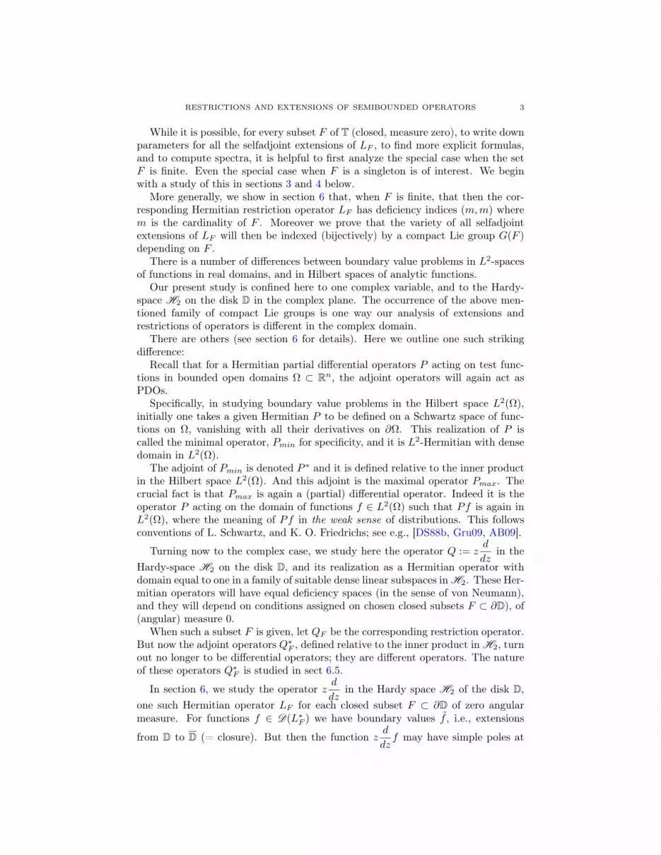
are as follows: For θ ∈ F , set
f(θ)± (z) :=
∞∑n=0
e(−n θ)n∓ i
zn; (6.39)
i.e., the expansion coefficients for f (θ)± are
f(θ)± (n) = e(n θ)x±(n), n ∈ N0. (6.40)
Then D±(LF ) is the closed span in H2 of the functions in (6.39), as θ ranges overF .
Proof. We will do the detailed steps for any f (θ)+ (·)
∣∣ θ ∈ F ⊂ D+(LF ), as theother case for D−(LF ) is the same argument, mutatis mutandis.
Note that functions ϕ ∈ D(LF ) are given by the condition
ϕ(θ) ' ϕ(e(θ)) = 0, ∀θ ∈ F (6.41)
where we use the usual identification θ ←→ e(θ) = ei2πθ with points in a periodinterval ' points in T. For ϕ ∈ D(LF ), set xn = ϕ(n), i.e., ϕ(z) =
∑n∈N0
xnzn. Then
for θ ∈ F , we have; (nxn) ∈ l2(N0), and:
0 = ϕ(θ) =
∞∑n=0
xne(n θ)
=
⟨e(n θ)
n− i, (n+ i)xn
⟩l2(N0)
=⟨f
(θ)+ , (LF + iI)ϕ
⟩H2
(6.42)
where, in the last step, we used the isomorphism l2(N0) 'H2 of Lemma 6.2. Therespective subscripts 〈·, ·〉l2(N0) and 〈·, ·〉H2
indicates the reference Hilbert spaceused.
Since (6.42) holds for all θ ∈ F , it follows that each f (θ)+ ∈ D(LF ), so the asserted
“=” in the Corollary follows.
Remark 6.17. If θ and ρ ∈ I (= the period interval), then the H2-inner product ofthe two functions f (θ)
+ and f (θ)− is as follows:⟨
f(θ)+ , f
(ρ)+
⟩H2
=
∞∑n=0
e(n(θ − ρ))
1 + n2= Z(θ − ρ, 1, 2) (6.43)
where Z is the Hurwitz-zeta function.
Theorem 6.18. Let the closed subset F ⊂ T be as in Corollary 6.16 and let LF bethe corresponding Hermitian unbounded and densely defined operator in the Hardyspace H2. Then each of the two defect spaces D±(LF ) in (6.38) is a reproducingkernel Hilbert space (RKHS) with RK equal to the Hurwitz zeta function (6.43).
Proof. For the theory of RKHS, see for example [Nel57, Alp92, ABK02]. In sum-mary, given a set F and a positive definite kernel K(α, β)(α,β)∈F×F then theRKHS, H (K) is the completion of finitely supported functions ϕ on F , i.e.,
ϕ : F → C (6.44)

RESTRICTIONS AND EXTENSIONS OF SEMIBOUNDED OPERATORS 38
in the pre-Hilbert inner product:
〈ϕ,ψ〉H (K) :=∑α
∑β
ϕ(α)ψ(β)K(α, β). (6.45)
The positive definite property in (6.45) is the assertion that
〈ϕ,ϕ〉H (K) =∑∑F×F
ϕ(α)ϕ(β)K(α, β) ≥ 0 (6.46)
for all finitely supported functions ϕ, see (6.44).To establish the theorem, take
K(α, β) =
∞∑n=0
e(n(α− β))
1 + n2= Z(α− β, 1, 2) (6.47)
where the expression in (6.47) is the Hurwitz zeta function.We will denote the Hurwitz zeta-function simply
Z(x) :=
∞∑n=0
e(nx)
1 + n2. (6.48)
Continue the proof now for D+(LF ) (the other case is by the same argument),recall from Corollary 6.16 that if ϕ is a finitely supported function on F (see (6.44)and (6.39)) then
(Tϕ) (z) =∑α∈F
ϕ(α)f(α)+ (z). (6.49)
By (6.49) and (6.45), we conclude that
‖Tϕ‖2H2= ‖ϕ‖2H (KHurwitz) .
But this means that T in (6.49) extends by closure and completion to become anisometric isomorphism of the RKHS H (K) onto D+(LF ) ⊂H2.
Lemma 6.19. Let Z be as in (6.43), and write
Z(x) =
∞∑n=0
e(nx)
1 + n2
=
∞∑n=0
cos(2πnx)
1 + n2+ i
∞∑n=1
sin(2πnx)
1 + n2
= f(x) + ig(x) (6.50)
where f := <(Z), and g := =(Z). Then
f(x) =π
2
∑n∈Z
e−2π|x+n| +1
2. (6.51)
Moreover, (f∣∣[0,1]
)(x) =
π
2
cosh(2π(x− 12 ))
sinh(π)+
1
2. (6.52)
Therefore, f is the 1-periodic extension of the RHS in (6.52).

RESTRICTIONS AND EXTENSIONS OF SEMIBOUNDED OPERATORS 39
Proof. From Remark 4.3, we see that
f(x) =
∞∑n=0
cos(2πnx)
1 + n2=π
2
cosh(2π(x− 12 ))
sinh(π)+
1
2, x ∈ [0, 1]. (6.53)
It is well-known that for causal sequences in l2(N0) 'H2, the real and imaginaryparts of the corresponding Fourier transform are related via the Hilbert transform.Thus, we have
g(θ) = p.v.ˆ 1
0
f(t) cot (π(θ − t)) dt (6.54)
where cot(π(θ − x)) is the Hilbert-kernel. See Figure 6.4 below.
ReHZL
ImHZL
-2 -1 1 2x
-0.5
0.5
1.0
1.5
2.0
Figure 6.4. The real and imaginary parts of the Hurwitz zeta-function Z(x). Note that Z(x) is real-valued at Z/2.
Let ψ(x) := e−2π|x|, so that
ψ(λ) =
ˆ ∞−∞
ψ(x)e−i2πλxdx =1
π
1
1 + λ2.
For any function f on R, define
(PERf) (x) :=∑n∈Z
f(x+ n).
It follows that (see [BJ02])
(PERψ) (x) =∑n∈Z
ψ(n)e(nx)
=1
π
∑n∈Z
e(nx)
1 + n2=
1
π+
2
π
∞∑n=1
cos(2πnx)
1 + n2. (6.55)
Eq. (6.51) follows from this.
RESTRICTIONS AND EXTENSIONS OF SEMIBOUNDED OPERATORS 40
For x ∈ [0, 1], we also have
(PERψ) (x) =∑n∈Z
e−2π|x+n|
= e−2πx∞∑n=0
e−2πn + e2πx∞∑n=1
e−2πn
=cosh(2π(x− 1
2 ))
sinh(π). (6.56)
Combine (6.51) and (6.56), we get the desired result in (6.52).
Lemma 6.20. The following Fourier integral identities hold:ˆ ∞0
cos(2πλx)
1 + λ2dλ = πe−2π|x| (6.57)
ˆ ∞0
sin(2πλ)
1 + λ2dλ =
1
2
(e−2πxli
(e2πx
)− e2πxli
(e−2πx
))(6.58)
where li(x) is the logarithmic integral
li(x) =
ˆ x
0
dt
ln t, x > 0; (6.59)
and for 0 < x < 1, the RHS in (6.59) denotes Cauchy principal value.
Proof. Eq. (6.57) can be verified directly. For (6.58), see [Boc59, page 67].
Corollary 6.21. Let Z be the Hurwitz zeta-function in (6.43), and let g = =(Z).Set
ϕ(x) :=1
2
(e−2πxli
(e2πx
)− e2πxli
(e−2πx
)); (6.60)
theng(x) = (PER ϕ) (x) =
∑n∈N
ϕ(x+ n). (6.61)
Proof. See [BJ02]. Figure 6.5 below illustrates the approximation
limN→∞
N∑n=−N
ϕ(x+ n) = g(x) (= =Z) .
Lemma 6.22. Hurwitz zeta-function is positive definite on R, i.e., if ϕ : R→ C isany finitely supported function on R, then∑
x
∑y
ϕ(x)ϕ(y)Z(x− y) ≥ 0. (6.62)
Proof. Computation of the double-sum in (6.62) yields
∞∑n=0
1
1 + n2
∣∣∣∣∣∑x
ϕ(x) e(nx)
∣∣∣∣∣2
≥ 0. (6.63)
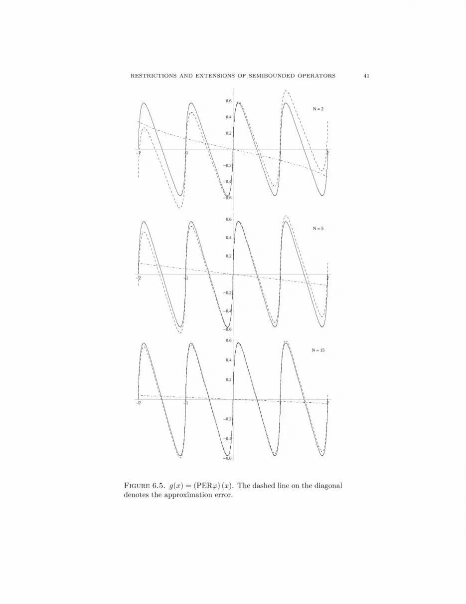
RESTRICTIONS AND EXTENSIONS OF SEMIBOUNDED OPERATORS 41
N = 2
-2 -1 1 2
-0.6
-0.4
-0.2
0.2
0.4
0.6
N = 5
-2 -1 1 2
-0.6
-0.4
-0.2
0.2
0.4
0.6
N = 15
-2 -1 1 2
-0.6
-0.4
-0.2
0.2
0.4
0.6
Figure 6.5. g(x) = (PERϕ) (x). The dashed line on the diagonaldenotes the approximation error.

RESTRICTIONS AND EXTENSIONS OF SEMIBOUNDED OPERATORS 42
The next results yield a representation of all the partial isometries between thetwo defect spaces determined by some chosen and fixed finite subset F of T, asin Corollary 6.13. But, by von Neumann’s classification (Lemma 1.1), this willthen also be a representation of all the selfadjoint extensions of the basic Hermitianoperator LF in (6.32) determined by the set F . If the cardinality of F ism, then theoperator LF has deficiency indices (m,m), and the partial isometries map betweenm-dimensional deficiency-spaces.
Corollary 6.23. Let Z be the Hurwitz zeta function from (6.50), and let F ⊂ Tbe a finite subset. Let
LF := Hf∈H2
∣∣ z ddz f∈H2, f=0 on F. (6.64)
Then the partial isometries UF between the two deficiency spaces D±(LF ) from thevon Neumann decomposition (1.3) in Lemma 1.1 are in bijective correspondencewith #F ×#F complex matrices (Mα,β)(α,β)∈F×F satisfying∑∑
(γ,ξ)∈F×F
Mγ,αZ(γ − ξ)Mξ,β = Z(α− β) (6.65)
for all (α, β) ∈ F × F .
Proof. In Theorem 6.18, we showed that each of the two deficiency spaces D±(LF )is an isomorphic image of the same RKHS, the one from the kernel
KZ(α, β) = Z(α− β) (6.66)
where Z = ZHurwitz is the Hurwitz zeta-function. Hence a partial isometry UF :D+(LF )→ D−(LF ), onto, will be acting on functions ϕ on F via the representation(6.49)
UF (∑α∈F
ϕ(α)f(α)+ ) =
∑α∈F
(Mϕ) (α)f(α)− (6.67)
where Mϕ on the RHS in (6.67) has the following matrix-representation:
(Mϕ) (α) =∑β∈F
Mα,βϕ(β). (6.68)
But we are also viewingM as an operator in l2(F ) which is finite-dimensional sinceF is assumed finite.
Substituting (6.68) into (6.67), and unravelling the isometric property of UF , thedesired conclusion (6.65) follows. To see this, notice (from Theorem 6.18) that∥∥∥∥∥∑
α∈Fϕ(α)f
(α)+
∥∥∥∥∥2
H2
=∑∑
(α,β)∈F×F
ϕ(α)ϕ(β)Z(α− β). (6.69)
Corollary 6.24. Let F ⊂ T be a finite subset (of distinct points), #F = m, andlet
KF (α, β) := Z(α− β) , (α, β) ∈ F × F (6.70)be the corresponding kernel defined from restricting the Hurwitz zeta-funciton Z.
(1) Then KF (·, ·) is (strictly) positive definite on the vector space VF = CF =all complex-valued functions on F , i.e., KF (·, ·) has rank #F .

RESTRICTIONS AND EXTENSIONS OF SEMIBOUNDED OPERATORS 43
(2) The (#F ) × (#F ) complex matrices M satisfying (6.65) form a compactLie group G(F ) of transformations in VF = CF .
Proof. Setm := #F . The key step in the proof is the assertion that the sesquilinearform KF (·, ·) in (6.70) has full rank, i.e., that its eigenvalues are all strictly positive.
Then it follows from Lie theory (see e.g., [Hel08]) that
G(F ) = M∣∣m×m complex matrix s.t. (6.65) holds (6.71)
is a compact Lie group as stated.It follows from (6.62) and (6.69) that KF (·, ·) is positive semi-definite. To show
that it has full rank = m, we must check that if ϕ ∈ VF = CF satisfying∑β∈F
KF (α, β)ϕ(β) = 0, ∀α ∈ F (6.72)
then ϕ = 0.Let ϕ ∈ VF satisfying (6.72). Using (6.69), note that (6.72) implies∑
β∈F
Z(α− β)ϕ(β) = 0, ∀α ∈ F, (6.73)
and therefore, by (6.63) ∑β∈F
ϕ(β)e(nβ) = 0, ∀n ∈ N0. (6.74)
Now index the points β in F as follows β1, . . . , βm, with corresponding ζj :=e(βj) = ei2πβj ,1 ≤ j ≤ m; and set Nm := 0, 1, 2, . . . ,m − 1; then the matrix(e(nβj)) 1≤j≤m, n∈Nm is a Vandermonde matrix
1 1 · · · · · · 1ζ1 ζ2 · · · · · · ζmζ21 ζ2
2 · · · · · · ζ2m
......
......
...ζm−11 ζm−1
2 · · · · · · ζm−1m
(6.75)
with determinant ∏1≤j<k≤m
(ζk − ζj) 6= 0.
Hence, translating back to the sesquilinear form KF , we conclude that KF isstrictly positive definite, and that, therefore G(F ) is a compact Lie group of m×mcomplex matrices.
We proved that whenever a finite subset F ⊂ T is chosen as above, and if M isan element in the corresponding Lie group G(F ), then there is a unique selfadjointextension HM corresponding to the partial isometry induced by M , acting betweenthe two deficiency spaces for LF . In the next result we compute the spectrum ofHM . Each HM has pure point spectrum as LF has finite deficiency indices (m,m)where m = (#F ). Since for finite index all selfadjoint extensions have the sameessential spectrum [AG93]; and as a result we have pure point-spectrum.

RESTRICTIONS AND EXTENSIONS OF SEMIBOUNDED OPERATORS 44
Example 6.25. Let the closed subset F of ∂D consist of the two points z± = ±1.Then the compact group G(F ) from Corollary 6.24 is (up to conjugacy) the groupof 2× 2 complex matrices preserving the quadratic form
C2 3 (z1, z2) 7→ Kev |z1|2 +Kodd |z2|2 (6.76)
where
Kev :=
∞∑n=0
1
1 + (2n)2, and
Kodd :=
∞∑n=0
1
1 + (1 + 2n)2;
(6.77)
i.e., the splitting of the summation∑k∈N0
=1
2(1 + π coth(π)) into even and odd
parts.
Proof. Computation of the Hurwitz zeta-function at the two points F = ±1yields the two numbers Kev and Kodd in (6.77).
Note 0 < Kodd < Kev. Hence when the matrix KZF in (6.47) is computed forF = ±1, we get for eigenvalues the two numbers in (6.77). The correspondingsystem of normalized eigenvectors in C2 is
1√2
(11
),
1√2
(1−1
).
The assertion in (6.77) follows from this.
Corollary 6.26. Let F ⊂ T be finite, and let M ∈ G(F ) where G(F ) is theLie group from Corollary 6.24. Then λ ∈ R is in the spectrum of the selfadjointextension HM if and only if there is some ψ ∈ CF (a complex valued function onF ) such that λ is a root in the following function
FM (λ) :=∑k∈N0
∑α∈F
e(kα)ψ(α)(λ− i)(k + i) + (Mψ) (α)(λ+ i)(k − i)
(k − λ) (k2 + 1). (6.78)
Moreover, we have
dFMdλ
(λ) =∑k∈N0
∑α∈F
e(kα)ψ(α) + (Mψ) (α)
(k − λ)2 . (6.79)
It follows that the selfadjoint extension HM has the same qualitative spectralconfiguration as we described in our results from section 4, which deal only with thespecial case of deficiency indices (1, 1). From our spectral generating function FMand its derivative, given above, it follows that the spectral picture in the (m,m) caseis qualitatively the same, now for m > 1, as we found in section 4 in the special caseof m = 1 : Only point-spectrum: and when one of the selfadjoint extensions HM isfixed, we get eigenvalues distributed in each of the intervals (−∞, 0), and [n, n+ 1)for n ∈ N0. But excluding (−∞, 0) for the case of the Friedrichs extension.
Proof. Now the partial isometries UM : D+(LF ) → D−(LF ) from Lemma 1.1 aregiven by CF 3 ϕ 7→ Mϕ ∈ CF via the formula (6.65) from Corollary 6.24, where

RESTRICTIONS AND EXTENSIONS OF SEMIBOUNDED OPERATORS 45
M ∈ G(F ). For ψ ∈ CF , set
f+(ψ) =∑α∈F
ψ(α)f(α)+ =
∑α∈F
(∑k∈N0
ψ(α)e(kα)
k − izk
)∈ D+(LF ); (6.80)
and
f−(ψ) =∑α∈F
ψ(α)f(α)− =
∑α∈F
(∑k∈N0
ψ(α)e(kα)
k + izk
)∈ D−(LF ). (6.81)
Using now the characterization of the selfadjoint extensions HM (M ∈ G(F )) ofthe initial operator LF , we get:
HM (g + f+(ψ) + f−(Mψ)) = Lg + i (f+(ψ)− f−(Mψ)) (6.82)
valid for all g ∈ D(LF ), and all ψ ∈ CF . Indeed by Lemma 1.2 the vectors f inD(HM ) must have the form
f = g + f+(ψ) + f−(Mψ) (6.83)
where g ∈ D(LF ), i.e., g(α) = 0, ∀α ∈ F , and where ψ ∈ CF . But (6.83) has anl2(N0)-representation as follows (k ∈ N0):
fk = gk +∑α∈F
ψ(α)e(kα)
k − i+∑α∈F
(Mψ) (α)e(kα)
k + i. (6.84)
For details on (Mψ)(α), see (6.67).Hence, the eigenvalue problem (for λ ∈ R)
HMf = λf, f ∈ D(HM ) (6.85)
takes the following form:
kgk + i∑α∈F
e(kα)
(ψ(α)
k − i− (Mψ) (α)
k + i
)= λgk + λ
∑α∈F
e(kα)
(ψ(α)
k − i+
(Mψ) (α)
k + i
); (6.86)
which in turn simplifies as follows: The function
FM (λ) =∑k∈N0
∑α∈F
e(kα)
(k − λ)
[λ
(ψ(α)
k − i+
(Mψ) (α)
k + i
)− i(ψ(α)
k − i− (Mψ) (α)
k + i
)]=
∑k∈N0
∑α∈F
e(kα)ψ(α)(λ− i)(k + i) + (Mψ) (α)(λ+ i)(k − i)
(k − λ) (k2 + 1).
So ψ ∈ CF must be such that the function
F(ψ)M (λ) =
∑k∈N0
∑α∈F
e(kα)ψ(α)(λ− i)(k + i) + (Mψ) (α)(λ+ i)(k − i)
(k − λ) (k2 + 1)(6.87)
has λ as a root, i.e., FM (λ) = 0 must hold for points λ ∈ spect(HM ); and converselyif FM (λ) = 0, then the vector f in (6.84) will be an eigenvector, note∑
k∈N0
gk e(kα) = 0, ∀α ∈ F.

RESTRICTIONS AND EXTENSIONS OF SEMIBOUNDED OPERATORS 46
We proceed to verify (6.79). Setting
A := ψ(α) (k + i)
B := (Mψ) (α) (k − i)
and
gk,α(λ) :=A(λ− i) +B(λ+ i)
(k − λ) (k2 + 1);
then from (6.78), we have
FM (λ) =∑k∈N0
∑α∈F
e(kα)gk,α(λ).
Note that
g′k,α(λ) =(A+B) k − i(A−B)
(k − λ)2
(k2 + 1), (6.88)
and the numerator in (6.88) is given by
(A+B) k − i(A−B)
= k (ψ(α) (k + i) + (Mψ) (α) (k − i))− i (ψ(α) (k + i)− (Mψ) (α) (k − i))= ψ(α) (k(k + i)− i(k + i)) + (Mψ) (α) (k(k − i) + i(k − i))= (ψ(α) + (Mψ) (α))
(k2 + 1
).
Substitute the above equation into (6.88), we get
g′k,α(λ) =(ψ(α) + (Mψ) (α))
(k2 + 1
)(k − λ)
2(k2 + 1)
=ψ(α) + (Mψ) (α)
(k − λ)2 .
It follows thatdFMdλ
=∑k∈N0
∑α∈F
g′k,α(λ)
=∑k∈N0
∑α∈F
e(kα)ψ(α) + (Mψ) (α)
(k − λ)2
which is eq. (6.79).Note in the computation of the derivative we get cancellation of the factor (k2+1)
in numerator and denominator.
6.4. A Comparison
Below we offer a comparison of the extension theory in the subspace L+ and inthe ambient Hilbert space L2(R/Z) ' L2(I), where we are using the usual identifi-cation between the quotient R/Z and a choice of a period interval I. There is a slightnotational ambiguity, as L may be understood as refer to a Hermitian operator withdense domain, referring each of the two Hilbert spaces L+ and L2(R/Z) ' L2(I),where I = [0, 1); see Table 1. But the boundary conditions f(0) = f(1) = 0 makesense in both cases; and in both cases, it is understood that f and d
dxf are in L2.

RESTRICTIONS AND EXTENSIONS OF SEMIBOUNDED OPERATORS 47
Lemma 6.27. Let L be the above mentioned Hermitian operator with dense domainD(L) in L2(R/Z). For ζ = e(θ) ∈ T, let Hθ(= Hζ) be the corresponding selfadjointextension; see the von Neumann classification, Lemma 1.1, and let H (θ) be theHilbert space:
f : R→ C measurable, and in L2loc; (6.89)
f(x+ n) = e(nθ)f(x), ∀x ∈ R,∀n ∈ Z; and (6.90)
‖f‖2H (θ) =
ˆR/Z|f(x)|2 dx <∞ (6.91)
(Note that the integral in (6.91) makes sense on account of (6.90), i.e., |f |2 is a1-periodic function on R. )
(1) Then for every θ, the restriction mapping H (θ)Tθ→ L2(I) is a unitary
isometric isomorphism, and
Uθ(t) = TθU(t)T ∗θ , t ∈ R, on L2(I) (6.92)
yields all the unitary one-parameter groups Uθ(t) corresponding to theselfadjoint extensions of L. In (6.90) RHS, U(t)t∈R is the periodic trans-lation f 7→ f(x+ t) acting in the Hilbert space H (θ).
(2) If θ ∈ [0, 1) is the parameter of the von Neumann classification, thenUθ(t)t∈R in (6.90) leaves invariant the subspace L+ if and only if θ = 0.
Proof. See the discussion above. The construction in (6.90) is an example of aninduced representation; induction from Z up to R; see [Mac88].
It follows from (6.92) that for fixed θ ∈ [0, 1) the spectrum of the unitary one-parameter group Uθ(t)t∈R and its selfadjoint generator Hθ in L2(I) ' L2(R/Z)is eθ+n
∣∣n ∈ Z, where eϕ(x) = e(ϕx) = ei2πϕx. Now let PL+ be the projection ofL2(I) onto L+, then a computation yields∥∥PL+
eϕ∥∥2
= 1− sin2(πϕ)
π2ζ1(ϕ).
see Lemma 6.28 and Figure 6.6 below. Apply this to ϕ = θ + n, and the lastconclusion in the lemma follows from this.
Lemma 6.28. Let
ζ1(ϕ) =
∞∑n=1
1
(ϕ+ n)2(6.93)
be the Hurwitz zeta function. (Note, the summation in (6.93) begins at n = 1.)Then ∥∥PL+
eϕ∥∥2
= 1− sin2(πϕ)
π2ζ1(ϕ). (6.94)
Proof. In the verification of (6.94), it is convenient to choose I = [− 12 ,
12 ) as period
interval in the duality of Lemma 6.2. For PL+eϕ we get
PL+eϕ =
∞∑n=0
〈en, eϕ〉L2(I) en
=
∞∑n=0
sinπ(ϕ− n)
π(ϕ− n)en; and

RESTRICTIONS AND EXTENSIONS OF SEMIBOUNDED OPERATORS 48
-4 -2 2 4j
0.2
0.4
0.6
0.8
1.0
Sin2 HΠ j L
Π2
Ζ1HjL
Figure 6.6. The function sin2(πϕ)π2 ζ1(ϕ)
therefore ∥∥PL+eϕ∥∥2
=
∞∑n=0
sin2(π(ϕ− n))
(π(ϕ− n))2 (by Parseval)
=sin2(πϕ)
π2
∞∑n=0
1
(ϕ− n)2 .
Now compare this to
1 = ‖eϕ‖2L2(I) =sin2(πϕ)
π2
∑n∈Z
1
(ϕ− n)2 ;
also by Parseval. Subtraction yields
1−∥∥PL+eϕ
∥∥2=
sin2(πϕ)
π2ζ1(ϕ). (6.95)
To get this, change variable in the summation range −∞ < n ≤ −1. The desiredconclusion (6.94) is now immediate from (6.95).
6.5. The Operator L∗
We now turn to von Neumann’s boundary theory for the Hermitian operatorsLF in the complex case (see Corollary 6.14), so the case when the Hilbert spaceis H2 (= the Hardy space). We already proved that the deficiency subspaces (inthe sense of von Neumann), are different from their analogues for boundary valueproblems in the real case, see e.g., Theorem 6.18. The two deficiency spaces areRKHSs, and they depend on conditions assigned on the prescribed closed subsetF ⊂ ∂D, of (angular) measure 0.
When such a subset F is fixed, let LF be the corresponding Hermitian operator.But now the adjoint operators L∗F , defined relative to the inner product in H2,turns out no longer to be differential operators. The nature of these operators L∗Fdepends on use of analytic function theory in an essential way, and it is studied

RESTRICTIONS AND EXTENSIONS OF SEMIBOUNDED OPERATORS 49
below. By analogy to the real case, one might guess that L∗F is again a differentialoperator acting on a suitable domain in H2, but it is not; – not even in the simplestcase when the set F is a singleton.
Lemma 6.29. Let L be the Hermitian operator as before, i.e., L is the restriction
of H = zd
dzon the dense domain D(L) in H2, consisting of functions f ∈ D(H)
s.t. f(1) = 0. On meromorphic functions f , set
(CP1f) (z) :=(
limw→1
(w − 1)f(w)) 1
z − 1(6.96)
=1
z − 1
1
2πi
˛γ at z=1
f(w)dw (6.97)
where the contour is chosen as a circle centered at z = 1. Then on its domain, asan operator, L∗ acts as follows:
L∗ = (1− CP1) zd
dz. (6.98)
Proof. Recall that in our model in the Hardy space, we have L ⊂ H ⊂ L∗ (see(3.4)), and
dim D(H)/D(L) = dim D(L∗)/D(H) = 1.
In particular, the two defect vectors (3.7) and (3.8) have the following representa-tion:
y2 =
(1
1 + n2
)n∈N0
7→ ρ2(z) :=
∞∑n=0
zn
1 + n2(6.99)
y3 =
(n
1 + n2
)n∈N0
7→ ρ3(z) :=
∞∑n=0
n zn
1 + n2. (6.100)
By von Neumann’s theory, the domain of L∗ is characterized by
D(L∗) =ϕ(z) + aρ2(z) + bρ3(z)
∣∣ ϕ ∈ D(L), and a, b ∈ C
; (6.101)
and
L∗ (ϕ(z) + aρ2(z) + bρ3(z)) = Lϕ(z) + aρ2(z) + bρ3(z)
= zd
dzϕ(z) + aρ3(z)− bρ2(z). (6.102)
Note for all z ∈ D, we have
zd
dzρ2(z) =
∞∑n=0
n zn
1 + n2= ρ3(z);
and
zd
dzρ3(z) =
∞∑n=0
n2 zn
1 + n2
= −∞∑n=0
zn
1 + n2+
∞∑n=0
zn
= −ρ2(z) +1
1− z.

RESTRICTIONS AND EXTENSIONS OF SEMIBOUNDED OPERATORS 50
As a result, for all f(z) = ϕ(z) + aρ2(z) + bρ3(z) ∈ D(L∗), we see that(zd
dzf
)(z) = z
d
dzϕ(z) + aρ3(z)− bρ2(z) +
b
1− z
= (L∗f) (z) +b
1− z. (6.103)
Now, the last term in the above equation has a simple pole at z = 1, and it isextracted by the map CP1 in (6.97) as follows:
b
1− z= CP1z
d
dzf. (6.104)
Hence (6.103) and (6.104) together yield
(L∗f) (z) =
(zd
dzf
)(z)− CP1z
d
dzf
= (1− CP1) zd
dzf(z)
which is (6.98).
Corollary 6.30. If g ∈ D(L∗) is such that zd
dzg ∈H2, then
L∗g = zd
dzg. (6.105)
Lemma 6.29 generalizes naturally to the operator LF , where the boundary con-ditions are specified by a finite subset F ⊂ T; see Corollaries 6.13 and 6.14.
Theorem 6.31. Let F = ζjmj=1 be a finite subset of T = ∂D. Let LF with domainD(LF ) be as Corollary 6.14. Specifically,
D(LF ) =
f ∈H2
∣∣ z ddzf ∈H2, f = 0 on F
. (6.106)
Recall LF has deficiency-indices (m,m). Set
(CPF (f)) (z) :=
m∑j=1
(limw→ζj
(w − ζj) f(w)
)1
z − ζj. (6.107)
Then L∗ acts on D(L∗) as follows:
L∗ = (1− CPF ) zd
dz. (6.108)
In justifying formula (6.108) we need the following
Lemma 6.32. Let F = ζjmj=1 ⊂ ∂D be as above, and let D(L∗F ) be the domainof the adjoint operator (LF )
∗ acting in H2.Then the functions in the subspace
GF :=
zd
dzf∣∣ f ∈ D(L∗F )
(6.109)
have the following properties:(1) Every g ∈ GF is analytic in D;(2) But not every g ∈ GF is in H2;

RESTRICTIONS AND EXTENSIONS OF SEMIBOUNDED OPERATORS 51
(3) The functions g ∈ GF are meromorphic with possible poles of order at mostone, and the poles are contained in F .
Proof. The justification of conclusions (1)-(3) in the lemma will follow from thecomputations below, but we already saw that
g(z) := zd
dzρ3(z) = −ρ2(z) +
1
1− z
holds, where ρ2 and ρ3 are the functions in (6.99)-(6.100). Note that g = zd
dzρ3 ∈ GF
where F = 1 is the singleton.
Proof of Theorem 6.31. See the proof of Lemma 6.29. In detail:The system of vectors
f(j)± (z) =
∞∑n=0
ζn
j
n∓ izn =
∞∑n=0
1
n∓ i(ζjz)n
(6.110)
is a generating system of vectors for the two deficiency spaces D(F )± for LF .
Introducing, R2(w, z) = ρ2(wz), and R3(w, z) = ρ3(wz) for z ∈ D, and w ∈ ∂D,we conclude that D+ + D− is spanned by the 2m functions
z 7→ R2(ζj , z) and z 7→ R3(ζj , z). (6.111)
Moreover,z ddzR3(ζj , z) = −R2(ζj , z) + 1
1−ζjz
z ddzR2(ζj , z) = R3(ζj , z), z ∈ D, i ≤ j ≤ m,
(6.112)
where we recall that the second term of the RHS in (6.112) is the Szegö-kernel,
KSz (ζj , z) =(1− ζjz
)−1= − ζj
z − ζj, z ∈ D, 1 ≤ j ≤ m. (6.113)
Hence, application of CPF (in (6.107)) to KSz (ζj , ·) yields
CPFKSz (ζj , z) = KSz (ζj , z), z ∈ D. (6.114)
Combining this with the arguments from the proof of Lemma 6.29, we nowconclude that the desired formula (6.108) holds on D(L∗F ) = D(LF ) + D+ + D−,where we used (6.110) and Corollary 6.16 in the last step.
Corollary 6.33. Let F = ζjmj=1 ⊂ T and LF be as in Theorem 6.31. Then theboundary form in (1.6) is given by
B(f, f) = =
m∑j=1
Cj(f)f(ζj)
(6.115)
for all f ∈ D(L∗), where
Cj(f) := limw→ζj
(w − ζj)(wd
dwf(w)
), j = 1, 2, . . . ,m; (6.116)
and f is the continuous extension of f onto the boundary ∂D. Note that Cj(f) is
the residue of zd
dzf at the simple pole z = ζj, j = 1, 2, . . . ,m.

RESTRICTIONS AND EXTENSIONS OF SEMIBOUNDED OPERATORS 52
Proof. By eq. (6.108), we have
〈L∗f, f〉 =
⟨zd
dzf, f
⟩−⟨CPF z
d
dzf, f
⟩〈f, L∗f〉 =
⟨f, z
d
dzf
⟩−⟨f, CPF z
d
dzf
⟩.
Note by (6.107) and (6.116), we see that
CPF zd
dzf(z) =
m∑j=1
Cj(f)KSz (ζj , z)
where KSz (ζj , z) is the Szegö-kernel (6.113).Hence
2iB(f, f) = 〈L∗f, f〉 − 〈f, L∗f〉
= 2i=⟨
f, CPF zd
dzf
⟩
= 2i=
m∑j=1
〈f, Cj(f)KSz (ζj , z)〉
= 2i=
m∑j=1
Cj(f)f(ζj)
and (6.115) follows from this.
7. The Friedrichs Extension
In sections 3 and 4 we introduced a particular semibounded operator L, and weproved that its deficiency indices are (1, 1). In section 6 we explored its relevancefor the study of an harmonic analysis in the Hardy space H2 of the complex diskD. We further proved that 0 is an effective lower bound for L (Lemma 5.1.) Wefurther proved that every selfadjoint extension of L has pure point-spectrum, uni-form multiplicity one. Moreover (Corollary 4.5), for every b < 0, we showed thatthere is a unique selfadjoint extension Hb of L such that b is the smallest eigenvalueof Hb.
Now, in general, for a semibounded Hermitian operator L, there are two distin-guished selfadjoint extensions with the same lower bound, the Friedrichs extension,and the Krein extension; and in general they are quite different. For example, inboundary-value problems, these two selfadjoint extensions correspond to Dirichletvs Neumann boundary conditions, respectively.
But for our particular operator L from sections 3 and 4, we show that the two theFriedrichs extension, and the Krein extension, must coincide. While this may beobtained from abstract arguments, nonetheless, it is of interest to compute explic-itly this unique extension. Indeed, the abstract characterizations in the literature([DS88b, Kre55, AG93, Gru09]) of the two, the Friedrichs extension and the Kreinextension, are given only in very abstract terms.
Moreover, in general, it is not true that when a semibounded selfadjoint operatorH is restricted, that its Friedrichs extension will coincide with H. But it is true for

RESTRICTIONS AND EXTENSIONS OF SEMIBOUNDED OPERATORS 53
our particular model operator H. We now turn to the details of the study of theselfadjoint extensions of L.
Let H = l2(N0), and define the selfadjoint operator H as in section 3,
(Hx)k = k xk, k ∈ N0 (7.1)
andD(H) = x ∈ l2
∣∣ k xk ∈ l2. (7.2)
On the dense domain
D0 := D(L) = x ∈ D(H)∣∣ ∑k∈N0
xk = 0, (7.3)
setL := H
∣∣D0, (7.4)
i.e., L is the restriction of H to the dense domain D0 specified in (7.3).
Lemma 7.1. For the domain of L∗ (the adjoint operator), we have
D(L∗) = D0 + Cy2 + Cy3 (7.5)
as a direct sum, where
(y2)k =1
1 + k2, k ∈ N0 (7.6)
and
(y3)k =k
1 + k2, k ∈ N0, (7.7)
see sect. 3.
Proof. The details for this formula (7.5) are contained in section 3.
Theorem 7.2. The operator H from (7.1)-(7.2) is the Friedrichs extension of L.
Proof. We denote the Friedrichs extension by HFriedrichs. On D0 from (7.3), wedefine the quadratic form
Q(x) := QL(x) = 〈x, Lx〉l2 + ‖x‖22 =∑k∈N0
k |xk|2 + ‖x‖22 , x ∈ D0. (7.8)
HenceQ(x) ≥ ‖x‖22 , for all x ∈ D0. (7.9)
Let HQ be the Hilbert completion of the pre-Hilbert space (D0, Q). Then from (7.9),we see that HQ is naturally contained in l2, i.e., containment with a contractiveembedding mapping HQ → l2, and bounded by 1; and moreover that (
√k xk) ∈ l2
holds for x ∈HQ. From [DS88a, p. 1240], we infer that
D(HFriedrichs) = D(L∗) ∩HQ. (7.10)
In addition to (7.10), we shall also need the following lemma.
Lemma 7.3. The selfadjoint operator H in (7.1) has as domain
D(H) = D0 + Cy2. (7.11)

RESTRICTIONS AND EXTENSIONS OF SEMIBOUNDED OPERATORS 54
Proof. ( ⊆ ) Let x ∈ l2 satisfy (7.2), and set
t :=∑k∈N0
1
1 + k2=
1
2(1 + π coth(π)) , and (7.12)
s :=∑k∈N0
xk; then (7.13)
z := x−(st
)y2 (7.14)
satisfies∑k∈N0
zk = 0.
Consequently, z ∈ D0, and therefore x ∈ RHS(7.11). Since y2 ∈ D(H), the otherinclusion “⊇” in (7.11) is clear.
We now continue with the proof of Theorem 7.2. We claim that the intersectionin (7.10) coincides with (7.11). Indeed, by (7.5), every x ∈ D(L∗) has the form
x = z + a y2 + b y3 (7.15)
where z ∈ D0, and a, b ∈ C. This decomposition is unique. If x is also in HQ, itfollows from (7.8)-(7.9) that x ∈ l2, and
(√k xk
)∈ l2. Since both terms z and a y2
satisfy the last condition, we conclude that the last term b y3 in (7.15) will as well.
But since√k (y3)k =
k3/2
1 + k2/∈ l2, we conclude that b = 0. Hence (7.15) reduces to
x = z + a y2; and this is in D(H) by Lemma 3.1. We proved that
D(H) = D(HFriedrichs)
and therefore H = HFriedrichs.
Corollary 7.4. Let the Hermitian operator L and its domain D(L) = D0 be as inTheorem 7.2, see also eq (3.3); then the Friedrichs and the Krein extensions of Lcoincide as selfadjoint operators in l2(N0).
Proof. For the definition of the Krein extension, see e.g., [AG93, sect. 107, p 367-8].To understand it, it is useful to introduce the following inner product on D(L∗) inthe general case of the von Neumann decomposition (1.5). For f, g ∈ D(L∗) set
〈f, g〉∗ = 〈f, g〉+ 〈L∗f, L∗g〉 . (7.16)
In this inner product 〈·, ·〉∗, the three subspaces D(L), and D± in (1.5) are mutuallyorthogonal, and, for f± ∈ D±, we have
‖f±‖2∗ = 〈f±, f±〉∗ = 2 ‖f±‖2 . (7.17)
Return now to the particular example with L in l2(N0) as described in thecorollary, and in Theorem 7.2, we introduce the standard ONB in l2(N0), en
∣∣ n ∈N0 where en(k) = δn,k for all n, k ∈ N0, and δn,k denoting the Kronecker-delta.
A computation shows that e0 ∈ D(L∗), and L∗e0 = 0.Clearly, e0 /∈ D(L). Moreover,
〈e0, x±〉∗ = ±i (7.18)
where (x±)n =1
n∓ iare the defect-vectors from (3.5).

RESTRICTIONS AND EXTENSIONS OF SEMIBOUNDED OPERATORS 55
We now define a selfadjoint extension K of L as follows
D(K) = D(L) + C e0 (7.19)
andK(ϕ+ c e0) = Lϕ (7.20)
for all ϕ ∈ D(L) and all c ∈ C.We see from (1.8), (7.17), and (7.18) that the co-dimension of D(L) in D(K) is
one. From (7.20), we get
〈ϕ+ c e0,K(ϕ+ c e0)〉 = 〈ϕ+ c e0, Lϕ〉= 〈ϕ,Lϕ〉+ c 〈e0, Lϕ〉= 〈ϕ,Lϕ〉+ c 〈L∗e0, ϕ〉= 〈ϕ,Lϕ〉 ≥ 0.
Since L has indices (1, 1), we conclude that the operator Kdefined in (7.19)-(7.20)is selfadjoint and semibounded, K ≥ 0; moreover Ke0 = 0, from (7.20).
We claim thatKen = n en, ∀n ∈ N0. (7.21)
This holds for n = 0. If n > 0, then en − e0 ∈ D(L), and
L(en − e0) = n en. (7.22)
Hence
Ken = K(en − e0 + e0)
= L(en − e0) by (7.20)
= n en by (7.22)
which is the desired conclusion (7.21).
Corollary 7.5. Among all the selfadjoint extensions of L in (7.3) and (7.4), theFriedrichs extension is the only one having its spectrum contained in [0,∞).
Proof. First note from Theorem 7.2 that spectrum(HFridrichs) = N0. But if Hθ isone of the other (different) selfadjoint extension of L in the von Neumann classifi-cation, we found in Theorem 4.4 that the spectrum has the form
λ0 < 0, n− 1 < λn < n, n = 1, 2, . . . (7.23)
with λn = λn(θ) depending on θ in the von Neumann classification. The conclusionfollows.
Corollary 7.6. Let L be the semibounded operator in (7.3) and (7.4) with defi-ciency indices (1, 1). Then for every selfadjoint extension Hθ in the von Neumannclassification we have resolvent operator
R(ξ,Hθ) = (ξI −Hθ)−1, =ξ 6= 0 (7.24)
in the Hilbert-Schmidt class.
Proof. From the eigenvalue list in (7.23) we note that∑n
∣∣∣(ξ − λn)−1∣∣∣2 <∞.

RESTRICTIONS AND EXTENSIONS OF SEMIBOUNDED OPERATORS 56
7.1. The Domain of the Adjoint Operator
In Lemma 7.1 and Theorem 7.2, we considered H = l2(N0), and a Hermitiansymmetric operator L with dense domain
D(L) =
x = (xk)k∈N0
∈ l2∣∣∣ (kxk) ∈ l2, and
∑k∈N0
xk = 0
. (7.25)
In consideration of the selfadjoint extensions of L, we used the domain D(L∗) andthe two vectors x± (see (3.5)), and the pair y2, y3 (see (7.6) & (7.7)), and
z = (zk)k∈N0, zk =
1
1 + k. (7.26)
These vectors all lie in D(L∗)\D(L); i.e., they are in the domain of the larger ofthe two operators, L ⊂ L∗. Recall
D(L∗)/D(L) = 2. (7.27)
The fact that special choices are needed results from the following:
Proposition 7.7. Let n ∈ N0, then the basis vectors en (en = (δn,k), k ∈ N0) arein D(L∗); and
L∗en = n en.
Moreover, the Friedrichs extension H of L is the unique selfadjoint extension s.t.en∣∣ n ∈ N0
⊆ D(H). (7.28)
Proof. Let y2, y3, and t :=∑k∈N0
11+k2 be as in (7.6), (7.7), and (7.12). Then set
en =
(en −
1
ty2
)︸ ︷︷ ︸∈D(L)
+1
ty2︸︷︷︸
∈D(L∗)
(7.29)
Since D(L) ⊂ D(L∗), it follows that en ∈ D(L∗).
Fix n. Since ϕ = en −1
ty2 satisfies
ϕk =
− 1
t (1 + k2)if k 6= n
1− 1
t (1 + n2)if k = n,
(7.30)
it follows that∑k∈N0
ϕk = 0, and so ϕ ∈ D(L). As a result, using L ⊂ L∗, we obtain
the following:
L∗en = Lϕ+1
tL∗y2. (7.31)
Now use L∗y2 = y3 (see section 3) in eq. (7.31) to compute L∗en as follows:If n, k ∈ N0, from (7.30) we obtain:
(L∗en) (k) =
− k
t(1 + k2)+
k
t(1 + k2)= 0 if k 6= n
n
(1− 1
t(1 + n2)
)+
n
t(1 + n2)= n if k = n.
RESTRICTIONS AND EXTENSIONS OF SEMIBOUNDED OPERATORS 57
Hence, (L∗en) (k) = nδn,k = nen(k); or L∗en = n en as asserted.
In Lemma 1.2 and (7.16), we introduced the graph-norm on D(L∗), i.e.,
‖f‖2∗ = ‖L∗f‖2 + ‖f‖2 , f ∈ D(L∗). (7.32)
The selfadjoint extensions H of L satisfy
L ⊆ H ⊆ L∗. (7.33)
Set‖f‖2H := ‖Hf‖2 + ‖f‖2 , f ∈ D(H). (7.34)
We now have the following result:
Proposition 7.8. Let L and H be as in (7.1) and (7.4). Then spanenn∈N isdense in D(H) w.r.t. the graph-norm ‖·‖H , but not dense in D(L∗) w.r.t. the othergraph-norm ‖·‖∗.
Proof. The first assertion in the proposition is clear (we say that spanen is acore for H.).
We now show that ρ3 ∼ y3 and ρ2 ∼ y2 are mutually orthogonal in D(L∗)relative to the inner product 〈·, ·〉∗ from (7.16) and (7.32).
Indeed, ρ3 ∈ D(L∗), and L∗ρ3 = −ρ2 (see (6.99) & (6.100)). Hence
〈ρ2, ρ3〉∗ = 〈ρ2, ρ3〉+ 〈L∗ρ2, L∗ρ3〉
= 〈ρ2, ρ3〉+ 〈ρ3,−ρ2〉 = 0.
Using the details from the proof of Corollary 7.4, we conclude that
ρ3 ∈ D(L∗)D(H) (7.35)
where in (7.35) refers to 〈·, ·〉∗.
Corollary 7.9. In the computation of L∗F in sect. 6, we must have a term not like
zd
dz; see Theorem 6.31.
8. Higher Dimensions
Now there is a higher dimensional version of our analysis in section 6 above (forthe Hardy-Hilbert space H2). This is the Arveson-Drury space H
(AD)d , d > 1.
While the case d > 1 does have a number of striking parallels with d = 1 fromsection 6, there are some key differences as well.
The reason for the parallels is that the reproducing kernel, the Szegö kernel(6.11), extends from one complex dimension to d > 1 almost verbatim. This is akey point of the Arveson-Drury analysis [Arv98, Dru78].
In section 6, for d = 1, we showed that the study of von Neumann boundarytheory for Hermitian operators translates into a geometric analysis on the boundaryof the disk D in one complex dimension, so on the circle ∂D.
It is the purpose of this section to show that multivariable operator theory ismore subtle. A main reason for this is a negative result by Arveson [Arv98, Coroll2] stating that the Hilbert norm in H
(AD)d , d > 1, cannot be represented by a Borel
measure on Cd. So, in higher dimension, the question of “geometric boundary” ismuch more subtle. Contrast this with eq (6.2) and Lemma 6.2 above.
The Szegö kernel Kw(z) = (1− wz)−1 (see (6.11)) in higher dimensions, i.e., Cdis called the Arveson-Drury kernel, see [Arv00, Arv98, Dru78].

RESTRICTIONS AND EXTENSIONS OF SEMIBOUNDED OPERATORS 58
Let z = (z1, . . . . , zd) ∈ Cd, α = (α1, . . . , αd) ∈ Nd0, i.e., αi ∈ N0; and set〈w, z〉 =
∑dj=1 wjzj ,
‖z‖2 =∑dj=1 |zj |
2,
(8.1)
and
K(AD)w (z) :=
1
1− 〈w, z〉. (8.2)
Then the corresponding reproducing kernel Hilbert space (RKHS) is called theArveson-Drury Hilbert space. It is a Hilbert space of analytic functions in
z = (z1, . . . . , zd) ∈ Bd =z ∈ Cd
∣∣ ‖z‖ < 1, (8.3)
(see (8.1).)Since, for d = 1,
zd
dzKw(z) =
wz
(1− wz)2 = wzKw(z)2,
zj∂
∂zjKw(z) = wjzjKw(z)2; and
in higher dimensions,d∑j=1
zj∂
∂zjKw(z) = 〈w, z〉Kw(z)2
= = −Kw(z) +Kw(z)2; (8.4)
it is natural to view H(AD)d as a direct extension of the Hardy space H2 from
section 6 above.But H
(AD)d is also a symmetric Fock space over the Hilbert space Cd, i.e.,
H(AD)d = Focksymm(Cd), see (8.1) and [Arv98].
Set Hj := zj∂
∂zj, and H :=
d∑j=1
Hj =
d∑j=1
zj∂
∂zj= the Arveson-Dirac operator,
andD(H) =
f ∈H
(AD)d
∣∣Hf ∈H(AD)d
. (8.5)
We know [Arv00] that Hj is a commuting family of selfadjoint operators inH
(AD)d .
For α = (α1, . . . , αd) ∈ Nd0, set n = |α| =d∑j=1
αj ; then(n
α
)=
n!
α1!α2! · · ·αd!are
the multinomial coefficients. It follows that
‖zα11 · · · z
αdd ‖
2
H(AD)d
=
(n
α
)−1
. (8.6)
Hence, iff(z) =
∑α∈Nd0
c(α)zα, (8.7)

RESTRICTIONS AND EXTENSIONS OF SEMIBOUNDED OPERATORS 59
zα := zα11 zα2
2 · · · zαdd , is in H
(AD)d , then
‖f‖2H
(AD)d
=
∞∑n=0
∑|α|=n
(n
α
)−1
|c(α)|2 . (8.8)
In H(AD)d , d > 1, the analogue of D(L) = D0, in Lemma 6.6, and Lemma 3.3, is
D0 =
f = fc ∈ D(H)∣∣ ∑α∈Nd0
c(α) = 0
. (8.9)
It is a dense linear subspace in H(AD)d .
Theorem 8.1. The operator familyHj
∣∣ 1 ≤ j ≤ dis a commuting family and
each Hj is essentially selfadjoint on D0.
Remark 8.2. Comparing the theorem with Lemma 6.6, and Corollary 6.13, we notethat the unitary one-parameter groups acting on H
(AD)d , d > 1, are more stable
than is the case for d = 1, (where the unitary one-parameter groups are acting inH2.) In short, “unitary motion” in Cd for d > 1 does not get trapped at “points.”
Proof of Theorem 8.1. To prove the theorem, we may use a result of Nelson [Nel59]showing now instead that
d∑j=1
H2j (8.10)
is essentially selfadjoint on D0.We must therefore show that, if g ∈H
(AD)d , and⟨
g,
I +
d∑j=1
H2j
fc
⟩H
(AD)d
= 0 (8.11)
for all fc ∈ D0, then it follows that g = 0.Hence, suppose (8.11) holds for some g ∈H
(AD)d , g(z) =
∑α∈N0
b(α)zα, then
∑α∈Nd0
(|α|α
)−1
b(α)
1 +
d∑j=1
α2j
c(α) = 0 (8.12)
for all fc ∈ D0.Consider α ∈ Nd0\(0) fixed, and set:
c(β) =
−1 β = (0, 0, . . . , 0)
1 β = α
0 β ∈ Nd0\0, α,(8.13)
and set n = |α|. Then, by (8.12), we have
b(α) = b(0)
(n
α
)1 +
d∑j=1
α2j
, (8.14)

RESTRICTIONS AND EXTENSIONS OF SEMIBOUNDED OPERATORS 60
and therefore (by (8.6) & (8.8)), that
‖g‖2H
(AD)d
= |b(0)|2∑α∈Nd0
(|α|α
)1 +
d∑j=1
α2j
2 . (8.15)
Since∑|α|=n
(n
α
)= dn, we conclude from (8.14) & (8.15) that b(0) = 0, and therefore
that g = 0 in H(AD)d .
Nelson’s theorem implies that∑dj=1H
2j is essentially selfadjoint on D0 (in (8.9)),
and the desired conclusion follows.
Acknowledgments
The co-authors, some or all, had helpful conversations with many colleagues,and wish to thank especially Professors Daniel Alpay, Ilwoo Cho, Dorin Dutkay,Alex Iosevich, Paul Muhly, Yang Wang, and Qingbo Huang. And going back intime, Bent Fuglede (PJ, SP), and Robert T. Powers, Ralph S. Phillips, DerekRobinson (PJ). The first named author was supported in part by the NationalScience Foundation, via a VIGRE grant.
References
[AB09] Daniel Alpay and Jussi Behrndt, Generalized Q-functions and Dirichlet-to-Neumannmaps for elliptic differential operators, J. Funct. Anal. 257 (2009), no. 6, 1666–1694.MR 2540988 (2010g:47077)
[ABK02] Daniel Alpay, Vladimir Bolotnikov, and H. Turgay Kaptanoğlu, The Schur algorithmand reproducing kernel Hilbert spaces in the ball, Linear Algebra Appl. 342 (2002),163–186. MR 1873434 (2002m:47019)
[AG93] N. I. Akhiezer and I. M. Glazman, Theory of linear operators in Hilbert space, DoverPublications Inc., New York, 1993, Translated from the Russian and with a prefaceby Merlynd Nestell, Reprint of the 1961 and 1963 translations, Two volumes boundas one. MR 1255973 (94i:47001)
[AHM11] S. Albeverio, R. Hryniv, and Y. Mykytyuk, Inverse scattering for discontinuousimpedance Schrödinger operators: a model example, J. Phys. A 44 (2011), no. 34,345204, 8. MR 2823449
[Alp92] Daniel Alpay, A theorem on reproducing kernel Hilbert spaces of pairs, Rocky Moun-tain J. Math. 22 (1992), no. 4, 1243–1258. MR 1201089 (94b:46035)
[Arv98] William Arveson, Subalgebras of C∗-algebras. III. Multivariable operator theory, ActaMath. 181 (1998), no. 2, 159–228. MR 1668582 (2000e:47013)
[Arv00] , The curvature invariant of a Hilbert module over C[z1, · · · , zd], J. ReineAngew. Math. 522 (2000), 173–236. MR 1758582 (2003a:47013)
[AS92] Milton Abramowitz and Irene A. Stegun (eds.), Handbook of mathematical functionswith formulas, graphs, and mathematical tables, Dover Publications Inc., New York,1992, Reprint of the 1972 edition. MR 1225604 (94b:00012)
[Bar49] V. Bargmann, On the connection between phase shifts and scattering potential, Rev.Modern Physics 21 (1949), 488–493. MR 0032069 (11,248g)
[BH08] Horst Behncke and D. B. Hinton, Eigenfunctions, deficiency indices and spectra ofodd-order differential operators, Proc. Lond. Math. Soc. (3) 97 (2008), no. 2, 425–449.MR 2439668 (2009g:34216)
[BJ02] Ola Bratteli and Palle Jorgensen, Wavelets through a looking glass, Applied and Nu-merical Harmonic Analysis, Birkhäuser Boston Inc., Boston, MA, 2002, The world ofthe spectrum. MR 1913212 (2003i:42001)
RESTRICTIONS AND EXTENSIONS OF SEMIBOUNDED OPERATORS 61
[BL10] Jussi Behrndt and Matthias Langer, On the adjoint of a symmetric operator, J. Lond.Math. Soc. (2) 82 (2010), no. 3, 563–580. MR 2739056 (2012c:47062)
[BMT11] Jussi Behrndt, Roland Möws, and Carsten Trunk, Eigenvalue estimates for singularleft-definite Sturm-Liouville operators, J. Spectr. Theory 1 (2011), no. 3, 327–347.MR 2831756
[Boc59] Salomon Bochner, Lectures on Fourier integrals. With an author’s supplement onmonotonic functions, Stieltjes integrals, and harmonic analysis, Translated by MorrisTenenbaum and Harry Pollard. Annals of Mathematics Studies, No. 42, PrincetonUniversity Press, Princeton, N.J., 1959. MR 0107124 (21 #5851)
[BV05] Pallav Kumar Baruah and M. Venkatesulu, Deficiency indices of a differential operatorsatisfying certain matching interface conditions, Electron. J. Differential Equations(2005), No. 38, 9 pp. (electronic). MR 2135249 (2006b:34074)
[Chu11] Nikolay L. Chuprikov, From a 1D completed scattering and double slit diffraction tothe quantum-classical problem for isolated systems, Found. Phys. 41 (2011), no. 9,1502–1520. MR 2823781
[CSLM11] Chao-Ping Chen, H. M. Srivastava, Li Li, and Seiichi Manyama, Inequalities andmonotonicity properties for the psi (or digamma) function and estimates for theEuler-Mascheroni constant, Integral Transforms Spec. Funct. 22 (2011), no. 9, 681–693. MR 2832199
[DHJ09] Dorin Ervin Dutkay, Deguang Han, and Palle E. T. Jorgensen, Orthogonal exponen-tials, translations, and Bohr completions, J. Funct. Anal. 257 (2009), no. 9, 2999–3019. MR 2559724 (2011a:42040)
[DJ07] Dorin Ervin Dutkay and Palle E. T. Jorgensen, Fourier frequencies in affine iter-ated function systems, J. Funct. Anal. 247 (2007), no. 1, 110–137. MR 2319756(2008f:42007)
[DJ11] , Affine fractals as boundaries and their harmonic analysis, Proc. Amer. Math.Soc. 139 (2011), no. 9, 3291–3305. MR 2811284
[dO09] César R. de Oliveira, Intermediate spectral theory and quantum dynamics, Progressin Mathematical Physics, vol. 54, Birkhäuser Verlag, Basel, 2009. MR 2723496
[Dru78] S. W. Drury, A generalization of von Neumann’s inequality to the complex ball, Proc.Amer. Math. Soc. 68 (1978), no. 3, 300–304. MR 480362 (80c:47010)
[DS88a] Nelson Dunford and Jacob T. Schwartz, Linear operators. Part I, Wiley ClassicsLibrary, John Wiley & Sons Inc., New York, 1988, General theory, With the assistanceof William G. Bade and Robert G. Bartle, Reprint of the 1958 original, A Wiley-Interscience Publication. MR 1009162 (90g:47001a)
[DS88b] , Linear operators. Part II, Wiley Classics Library, John Wiley & Sons Inc.,New York, 1988, Spectral theory. Selfadjoint operators in Hilbert space, With theassistance of William G. Bade and Robert G. Bartle, Reprint of the 1963 original, AWiley-Interscience Publication. MR 1009163 (90g:47001b)
[DS01] Harry Dym and Lev A. Sakhnovich, On dual canonical systems and dual matrix stringequations, Operator theory, system theory and related topics (Beer-Sheva/Rehovot,1997), Oper. Theory Adv. Appl., vol. 123, Birkhäuser, Basel, 2001, pp. 207–228.MR 1821914 (2003d:47063)
[EMOT81] Arthur Erdélyi, Wilhelm Magnus, Fritz Oberhettinger, and Francesco G. Tricomi,Higher transcendental functions. Vol. I, Robert E. Krieger Publishing Co. Inc., Mel-bourne, Fla., 1981, Based on notes left by Harry Bateman, With a preface by MinaRees, With a foreword by E. C. Watson, Reprint of the 1953 original. MR 698779(84h:33001a)
[Gil72] Richard C. Gilbert, Spectral representation of selfadjoint extensions of a symmetricoperator, Rocky Mountain J. Math. 2 (1972), no. 1, 75–96. MR 0290147 (44 #7332)
[Gru09] Gerd Grubb, Distributions and operators, Graduate Texts in Mathematics, vol. 252,Springer, New York, 2009. MR 2453959 (2010b:46081)
[Hel08] Sigurdur Helgason, Geometric analysis on symmetric spaces, second ed., Mathemat-ical Surveys and Monographs, vol. 39, American Mathematical Society, Providence,RI, 2008. MR 2463854 (2010h:22021)
[JPT11a] Palle Jorgensen, Steen Pedersen, and Feng Tian, Momentum Operators in Two In-tervals: Spectra and Phase Transition (submitted) http://arxiv.org/abs/1110.5948v1.

RESTRICTIONS AND EXTENSIONS OF SEMIBOUNDED OPERATORS 62
[JPT11b] , Translation Representations and Scattering By Two Intervals (submitted)http://arxiv.org/abs/1201.1447.
[Kat95] Tosio Kato, Perturbation theory for linear operators, Classics in Mathematics,Springer-Verlag, Berlin, 1995, Reprint of the 1980 edition. MR 1335452 (96a:47025)
[KN89] M. G. Kreın and A. A. Nudel′man, Some spectral properties of a nonhomogeneousstring with a dissipative boundary condition, J. Operator Theory 22 (1989), no. 2,369–395. MR 1043733 (91h:47048)
[Kre55] M. G. Krein, On some cases of the effective determination of the density of a nonuni-form string by its spectral function, 2 Pine St., West Concord, Mass., 1955, Translatedby Morris D. Friedman. MR 0075403 (17,740f)
[Kre70] M. G. Kreın, Čebyšev-Markov inequalities in the theory of the spectral functions of astring, Mat. Issled. 5 (1970), no. vyp. 1 (15), 77–101. MR 0284863 (44 #2087)
[Mac88] George W. Mackey, Induced representations and the applications of harmonic analysis,Harmonic analysis (Luxembourg, 1987), Lecture Notes in Math., vol. 1359, Springer,Berlin, 1988, pp. 16–51. MR 974302 (90c:22021)
[Mar11] R. T. W. Martin, Representation of simple symmetric operators with deficiency indices(1, 1) in de Branges space, Complex Anal. Oper. Theory 5 (2011), no. 2, 545–577.MR 2805419
[Mik04] V. A. Mikhaılets, The general spectrum of a family of selfadjoint extensions, Dopov.Nats. Akad. Nauk Ukr. Mat. Prirodozn. Tekh. Nauki (2004), no. 1, 18–21. MR 2107793(2006h:47040)
[Min04] V. S. Mineev, Physics of selfadjoint extensions: the one-dimensional scattering prob-lem for Coulomb potential, Teoret. Mat. Fiz. 140 (2004), no. 2, 310–328. MR 2101710(2005h:81414)
[MK08] R. Martin and A. Kempf, Approximation of bandlimited functions on a non-compactmanifold by bandlimited functions on compact submanifolds, Sampl. Theory SignalImage Process. 7 (2008), no. 3, 281–292. MR 2493860 (2010g:42006)
[Naz08] S. A. Nazarov, Selfadjoint extensions of the operator of the Dirichlet problem in athree-dimensional domain with an edge, Sib. Zh. Ind. Mat. 11 (2008), no. 1, 80–95.MR 2535251 (2010h:35065)
[Nel57] Edward Nelson, Kernel functions and eigenfunction expansions, Duke Math. J. 25(1957), 15–27. MR 0091442 (19,969f)
[Nel59] , Analytic vectors, Ann. of Math. (2) 70 (1959), 572–615. MR 0107176 (21#5901)
[Oro05] Yu. B. Orochko, Deficiency indices of an even-order one-term symmetric differen-tial operator that degenerates inside an interval, Mat. Sb. 196 (2005), no. 5, 53–82.MR 2154782 (2006d:47081)
[PR76] Robert T. Powers and Charles Radin, Average boundary conditions in Cauchy prob-lems, J. Functional Analysis 23 (1976), no. 1, 23–32. MR 0450732 (56 #9025)
[Rud87] Walter Rudin, Real and complex analysis, third ed., McGraw-Hill Book Co., NewYork, 1987. MR 924157 (88k:00002)
[Sad06] I. V. Sadovnichaya, A new estimate for the spectral function of a selfadjoint extensionin L2(R) of the Sturm-Liouville operator with a uniformly locally integrable potential,Differ. Uravn. 42 (2006), no. 2, 188–201, 286. MR 2246943 (2007e:34155)
[Sak97] L. A. Sakhnovich, Deficiency indices of a system of first-order differential equations,Sibirsk. Mat. Zh. 38 (1997), no. 6, 1360–1361, iii. MR 1618473 (98k:34133)
[ŞB11] Hamdullah Şevli and Necdet Batır, Complete monotonicity results for some functionsinvolving the gamma and polygamma functions, Math. Comput. Modelling 53 (2011),no. 9-10, 1771–1775. MR 2782863
[Šmu74] Ju. L. Šmul′jan, Closed Hermitian operators and their selfadjoint extensions, Mat.Sb. (N.S.) 93(135) (1974), 155–169, 325. MR 0341161 (49 #5911)
[ST10] Luis O. Silva and Julio H. Toloza, On the spectral characterization of entire opera-tors with deficiency indices (1, 1), J. Math. Anal. Appl. 367 (2010), no. 2, 360–373.MR 2607264 (2011d:47053)
[Vas07] F.-H. Vasilescu, Existence of the smallest selfadjoint extension, Perspectives in opera-tor theory, Banach Center Publ., vol. 75, Polish Acad. Sci., Warsaw, 2007, pp. 323–326.MR 2341359
RESTRICTIONS AND EXTENSIONS OF SEMIBOUNDED OPERATORS 63
[VGT08] B. L. Voronov, D. M. Gitman, and I. V. Tyutin, Construction of quantum observablesand the theory of selfadjoint extensions of symmetric operators. III. Selfadjoint bound-ary conditions, Izv. Vyssh. Uchebn. Zaved. Fiz. 51 (2008), no. 2, 3–43. MR 2464732(2009j:47161)
[vN32a] J. von Neumann, Über adjungierte Funktionaloperatoren, Ann. of Math. (2) 33 (1932),no. 2, 294–310. MR 1503053
[vN32b] , Über einen Satz von Herrn M. H. Stone, Ann. of Math. (2) 33 (1932), no. 3,567–573. MR 1503076
[YL11] Qiao-Hua Yang and Bao-Sheng Lian, On the best constant of weighted Poincaréinequalities, J. Math. Anal. Appl. 377 (2011), no. 1, 207–215. MR 2754820(2012a:35007)
(Palle E.T. Jorgensen) Department of Mathematics, The University of Iowa, IowaCity, IA 52242-1419, U.S.A.
E-mail address: [email protected]: http://www.math.uiowa.edu/~jorgen/
(Steen Pedersen) Department of Mathematics, Wright State University, Dayton,OH 45435, U.S.A.
E-mail address: [email protected]: http://www.wright.edu/~steen.pedersen/
(Feng Tian) Department of Mathematics, Wright State University, Dayton, OH45435, U.S.A.
E-mail address: [email protected]: http://www.wright.edu/~feng.tian/