OPTIMAL CONTROL APPLICATIONS AND METHODSOptim. Control Appl. Meth. 2010; 31:351–364Published online 1 September 2009 in Wiley InterScience (www.interscience.wiley.com). DOI: 10.1002/oca.909

Sequential quadratic programming and analytic hierarchy process for nonlinearmultiobjective optimization of a hydropower network

S. Ali A. Moosavian∗,†,‡, Ali Ghaffari§ and Amir Salimi¶

Department of Mechanical Engineering, Advanced Robotics and Automated Systems (ARAS) Laboratory,K. N. Toosi University of Technology, Tehran, Iran

SUMMARY

In this paper, an optimal annual scheduling for power generation (i.e. rule curves and volume of water releases) in serialor parallel hydropower plants is developed. Multiobjective programming and weighted sum method are used to converta multiobjective problem to a single objective one. Furthermore, to obtain viable alternatives under existing uncertainty,some random weight vectors in the whole weighting space are generated and for each weight vector an optimal solutionis found using sequential quadratic programming (SQP). Then, analytic hierarchy process (AHP) is used to select the bestsolution according to a given criterion, and determine the most preferred one. Besides, this method does not require choosinga priori preference for the objective function, thus making an ideal tool for handling complicated multiobjective modelsand easy to use with the aid of computer programs. Combination of multiobjective optimization and multicriteria decisionanalysis (MCDA) is an integrated methodology that is capable of dealing with complex water management problems.Various scenarios for dry, median, and wet years are assumed based on stochastic flows from external sources (e.g. floodingrivers, unexpected rains, etc.) coming into each reservoir, and turbine power generation is obtained from hill diagramsprovided by the manufacturer. The application of this methodology is illustrated in a case study for optimal scheduling ofKaroon River Basin, where the decision support system and optimization routines are implemented in MATLAB. The totalenergy productions for 10 optimized solutions under dry, median, and wet scenarios (generated from forty-year historicalinflow records) are calculated, and specific water consumption for each reservoir is obtained in different months. Thiscan significantly help decision makers to have an optimal and more intelligent management over energy productions inhydropower plants and associated thermal power plants. Copyright q 2009 John Wiley & Sons, Ltd.

Received 25 May 2008; Revised 30 May 2009; Accepted 22 June 2009

KEY WORDS: multiobjective optimization; stochastic-weighted sum method; sequential quadratic programming;multicriteria decision analysis; analytical hierarchy process

∗Correspondence to: S. Ali A. Moosavian, Department of Mechan-ical Engineering, #19 Pardis Alley, Sadra Street, Vanak Square,19991 43344, PO Box: 19395-199, K. N. Toosi University ofTechnology, Tehran, Iran.

†E-mail: moosavian@kntu.ac.ir‡Associate Professor.§Professor.¶Graduate student.

1. INTRODUCTION

The optimal annual operational scheduling ofhydropower plants and reservoirs network has becomeone of the most important subjects for electric powergeneration companies over the last decades. The aimis determining the reservoirs water release volumein each period (e.g. a month, a season, etc.) and

Copyright q 2009 John Wiley & Sons, Ltd.

352 S. A. A. MOOSAVIAN, A. GHAFFARI AND A. SALIMI

reservoirs storages at the beginning of each periodthat (under technological and operational constraints)maximizes operational benefit and performance (i.e.rule curves), and minimizes water spillage over ahorizon time (e.g. a year). Owing to existence ofuncertainties in optimization problem input data (likerandom water inflows to reservoirs) and nonlineari-ties in problem formulation, the optimal hydropowerplants operational scheduling problem is thus a largecomplex multiobjective and multivariable with variousconstraints optimization problem. Therefore, to solvethis problem a highly rational mathematical modelingof hydropower plant operation is required. Applyingmathematical modeling and various optimization tech-niques for solving these kinds of optimal problemsare developed by many authors in recent years. Thesetechniques include linear programming (LP), nonlinearprogramming (NLP), dynamic programming (DP),stochastic dynamic programming (SDP), and heuristicprogramming such as Genetic algorithms, Fuzzy logic,and Neural Networks [1–6].

Optimization models are based on explicitly spec-ified objective functions, criteria for evaluation ofoptimal results, and constraints as limitations [7].Multiobjective function solving techniques can becategorized into two major classes: (i) Aggregationapproaches; (ii) Pareto domination approaches. Usingobjective functions to evaluate the preferences ofthe defined objectives and the dominance of solutionsets is commonly expressed in aggregation approach.On the other hand, when no priority information isinvestigated or is available before the search, Paretodomination approach is commonly used [8]. Paretodomination approach is based on whether one solutionis dominated by others instead of a single compar-ative value [9]. The set of Pareto optimal solutionspresents the trade-off among the different objectives.A Pareto solution is the one for which any improve-ment in one objective can only take place if at leastother objective deteriorates [10, 11]. Various multi-objective optimization algorithms have been appliedbased on the Pareto domination approach [12, 13].Whereas a single solution could not optimize allobjective functions, the final solution of a multiob-jective problem should be one of the accord choicesthat can best satisfy the decision makers’ preferences.

Multiobjective methods can be divided into three maincategories based on acquiring the preference informa-tion procedures and using that in decision analysisprocesses [14]:

(i) Priori articulation of preference information,(ii) Progressive articulation of preference informa-

tion,(iii) Posteriori articulation of preference informa-

tion.

Priori articulation of the decision-makers’ preferencesis the most popular way that means different objectivesare converted to a single item before accomplishingthe actual optimization operation. Various approachesin this field have been proposed, including weightedsum [15], utility theory [16], acceptability functions[17, 18], goal programming [19–21], non-linear combi-nation [22, 23], and fuzzy logic [24–26]. Among thesemethods weighted-sum is the most conventional one.However, it could get only one or a few Pareto solu-tions and could not generate a set of Pareto solutions.Among various attempts made to get a set of Paretosolutions using the weighted sum method in one singlerun, choosing random weight (i.e. different combina-tions of the weights) is the general approach to obtaina set of Pareto solutions [27–29].

Multicriteria decision analysis (MCDA) method is a‘divide and conquer’ strategy that is used to reassemblethe parts to present a coherent overall image to decision-makers and subdivides a complicated result into parts toseparately deal easily. MCDA includes many differenttypes of procedures, such as a technique for order pref-erence by similarity to ideal solution, AHP, outrankingmethods, Elimination Et Choice Translating Realityand PROMETHEE. The AHP technique is a flexibledecision making tool for multiobjective problems, andhas been employed in the evaluation model [30–32].It enables decomposition of a problem into a hier-archy, and assures that both qualitative and quantita-tive aspects of the considered problem are incorporatedin the evaluation process. It is composed of severalpreviously existing but unassociated concepts and tech-niques such as hierarchical structuring of complexity,pair wise comparisons, redundant judgments, an eigen-vector method for deriving weights with consistencyconsiderations.

Copyright q 2009 John Wiley & Sons, Ltd. Optim. Control Appl. Meth. 2010; 31:351–364DOI: 10.1002/oca

SEQUENTIAL QUADRATIC PROGRAMMING AND ANALYTIC HIERARCHY PROCESS 353

Here, weighted sum method with formation ofrandom weight vectors, and AHP is applied to over-come hydropower generation scheduling complexities.The results are used to a field case study in KaroonRiver Basin. The advantages of the presented optimiza-tion method versus other works are using a combinationof multiobjective optimization and MCDA. Thiscombination offers decision makers a methodologyto quantify the qualitative knowledge in complicatedplanning problems, and could help them obtain prac-tical alternatives under various uncertainties. Also,using AHP permits decision makers to apply their idealindicators to specify best solution. Furthermore, usinga sixth-order polynomial to express forebay and tail-race water levels instead of constant values, to obtainactual power generation from turbine hill diagram withassuming forbidden operation zones instead of usingtheoretical formula, make the presented hydropowerplant model more operative than previous models withconstant water levels. Also, the value of energy genera-tion in different months is included in the optimizationmodel and specific water consumption is introducedas an important parameter to reach optimal operationof a hydropower network that has been rarely used byother authors.

In this study, first a description of AHP method andsequential quadratic programming (SQP) algorithmwill be presented. In Section 3, an optimization modelis developed and corresponding objective functions andconstraints are introduced. Next, the results obtainedfrom application of this research to Karoon Riverhydropower network are illustrated. The total energyproduction for 10 optimized solutions under dry,median, and wet scenarios is calculated, and specificwater consumption for each reservoir is obtained indifferent months.

2. OPTIMIZATION METHODOLOGY

2.1. Stochastic-weighted sum method

Assume that f(x)=( f1(x), f2(x), . . . , fk(x))T as criteriavector includes k objective functions that belong toa feasible region R f (1×k), and x=(x1, x2, . . . , xn)T

includes decision variables where x∈ Rx (1×n).

Various objective functions are calculated in theircorresponding different units and most of them havedifferent order of magnitudes. So, it is desirable thatthe ranges of different criteria become roughly equal,using a scaling method for the objective function.Three methods are available for scaling the objectivefunctions: (a) Normalization, (b) Using of 10 raisedto an appropriate power, (c) Application of rangeequalization factors [10]. Here, normalization methodis used.

If x∗ ∈ Rx is considered as an optimal variable vector,then f∗ ∈ R f is an optimal solution corresponding to x∗.Components f ∗

i (i=1,2, . . . ,k) of ideal criterion vector(f∗ ∈ R f ) are obtained by maximizing each of the objec-tive functions individually subjected to correspondingconstraints. So, a payoff matrix is formed by using thedecision vectors obtained when calculating the idealcriterion vector. On the i th row of the payoff matrixthere are values of all objective functions calculatedat the point where fi has its maximum value. Payoffmatrix can be expressed as follows:

F=

⎡⎢⎢⎢⎢⎢⎣

f1(x∗1) f2(x∗

1) · · · fk(x∗1)

f1(x∗2) f2(x∗

2) fk(x∗2)

......

...

f1(x∗k) f2(x∗

k) · · · fk(x∗k)

⎤⎥⎥⎥⎥⎥⎦k×k

(1a)

Denoting fi (x∗i ) by f ∗

i , then f∗ is at the main diagonalof the matrix. The minimal value of the i th columnin the payoff matrix is selected as an estimate of thelower bound of the i th objective ( f Li ) over the Paretooptimal solutions. According to the payoff matrix, eachobjective function fi (x)(i=1,2, . . . ,k) is replaced bya function as follows:

�( fi (x))= fi (x)− f Lif ∗i − f Li

(1b)

In this case, the range of each new objective function is[0,1]. In order to generate uniform distribution weightvectors, the weight interval of one objective function(i.e. independent objective function) is divided into jsubintervals. Suppose a problem with two objectivefunctions where the first objective f1(x) is an inde-pendent one and the weight interval of (0,1) has been

Copyright q 2009 John Wiley & Sons, Ltd. Optim. Control Appl. Meth. 2010; 31:351–364DOI: 10.1002/oca

354 S. A. A. MOOSAVIAN, A. GHAFFARI AND A. SALIMI

uniformly divided into j subintervals. The weight forf1(x) (expressed with � j

1) could be selected randomlyin j th interval, and then the weight for f2(x) couldbe decided by � j

2 =1−� j1. The set of Pareto solutions

can be obtained by solving batches of weighted sumproblems as follows:

Minimizek∑

i=1�i�( fi (x)) where �i�0 and

k∑i=1

�i =1

It should be noted that if an objective function fi is tobe maximized, it is equivalent to minimize (− fi ).

2.2. AHP evaluation model

2.2.1. Multiobjective decision analysis. Suppose thereare n optimized solutions that need to be ranked. Eachsolution has m performance indicators. Then the indexmatrix can be expressed as follows [33]:

Pm×n =[pij] (2)

where pij is the i th index of the j th solution,i=1,2, . . . ,m and j =1,2, . . . ,n. According to thecharacteristics of the performance indicators, thesolutions could be classified into two types:

(I) The biggest index value, the largest optimalmembership degree;

(II) The biggest objective value, the least optimalmembership degree;

These two types can be described as

(rij)I = pijmax(pi1, pi2, . . . , pin)

(3a)

(rij)II = min(pi1, pi2, . . . , pin)

pij(3b)

Then, the index matrix can be transferred to a member-ship degree matrix based on Equations (3a) and (3b):

Rm×n =[rij] (4)

where rij is the membership degree of the i th indexof the j th solution, i=1,2, . . . ,m and j =1,2, . . . ,n.

From the above definitions, 1 and 0 are the extremevalues of the membership function. The ideal andinferior vectors are denoted by I=(1,1, . . . ,1)T andJ=(0,0, . . .0)T, respectively. If the preference indiceshave different weights, then the weighting vector canbe expressed as:

x=(�1,�2, . . . ,�m)T,m∑j=1

� j =1 (5)

From matrix R, membership function vector r j =(r1 j ,r2 j , . . . ,rmj)T can be obtained for solution j . Thedistance between r j and I is given by:

‖r j −I‖P ={

m∑i=1

(�i |rij−1|)P}1/P

(6)

The distance between r j and J is:

‖r j −J‖P ={

m∑i=1

(�i |rij−0|)P}1/P

(7)

When P=2, the distance is also known as the generalEuclidean weighted distance.

Assuming that the relative optimal membershipdegree is chosen and denoted by z j , then the relativeoptimal membership degree to the inferiority can bedenoted by 1−z j . In order to obtain the optimalvalue of the relative optimal membership degree forthe j th solution z j and 1−z j can be viewed asweights. Thus, optimal membership degree functioncan be expressed as:

H(z j ) = z2j

{m∑i=1

(�i |rij−1|)P}2/P

+(1−z j )2{

m∑i=1

(�i rij)P}2/P

(8)

where z j that minimizes H(z j ) is desired for a decision-maker. Therefore:

dH(z j )

dz j=0

Copyright q 2009 John Wiley & Sons, Ltd. Optim. Control Appl. Meth. 2010; 31:351–364DOI: 10.1002/oca

SEQUENTIAL QUADRATIC PROGRAMMING AND ANALYTIC HIERARCHY PROCESS 355

Then, the optimal membership degree of solution Pj isobtained as follows:

z j = 1

1+[∑m

i=1 (�i |rij−1|)P∑mi=1 (�i rij)P

]2/P (9)

2.2.2. Hierarchical structure. The AHP is a type ofMCDA procedure where the key feature is a perfor-mance matrix, or consequence table. Each row of thetable describes an indicator, and each column describesthe performance of the options against each indicator,or the solutions. Commonly, MCDA techniques applynumerical analysis to a performance matrix in twostages:

(a) Scoring: the expected consequences of eachoption are assigned a numerical score on strengthof preference scale for each option and eachindicator. More preferred options score higheron the scale and less preferred options scorelower.

(b) Weighting: numerical weights are assigned foreach indicator to define the relative valuations ofa shift between the top and bottom of the chosenscale.

The AHP evaluation model is scored by the member-ship degree, which was described in Equation (3), andthe weighting vector in Equation (5) is used to showthe chosen scale of each indicator. Finally, optimizedsolutions can be ranked according to value of z j inEquation (9).

3. OPTIMIZATION MODEL

3.1. System dynamics

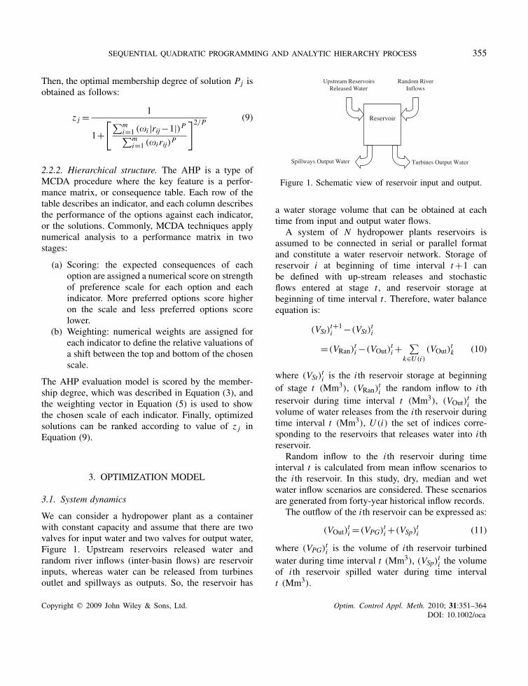
We can consider a hydropower plant as a containerwith constant capacity and assume that there are twovalves for input water and two valves for output water,Figure 1. Upstream reservoirs released water andrandom river inflows (inter-basin flows) are reservoirinputs, whereas water can be released from turbinesoutlet and spillways as outputs. So, the reservoir has

Reservoir

Upstream Reservoirs Released Water

Random River Inflows

Spillways Output Water Turbines Output Water

Figure 1. Schematic view of reservoir input and output.

a water storage volume that can be obtained at eachtime from input and output water flows.

A system of N hydropower plants reservoirs isassumed to be connected in serial or parallel formatand constitute a water reservoir network. Storage ofreservoir i at beginning of time interval t+1 canbe defined with up-stream releases and stochasticflows entered at stage t , and reservoir storage atbeginning of time interval t . Therefore, water balanceequation is:

(VSt)t+1i −(VSt)

ti

=(VRan)ti −(VOut)

ti +

∑k∈U (i)

(VOut)tk (10)

where (VSt)ti is the i th reservoir storage at beginningof stage t (Mm3), (VRan)ti the random inflow to i threservoir during time interval t (Mm3), (VOut)ti thevolume of water releases from the i th reservoir duringtime interval t (Mm3), U (i) the set of indices corre-sponding to the reservoirs that releases water into i threservoir.

Random inflow to the i th reservoir during timeinterval t is calculated from mean inflow scenarios tothe i th reservoir. In this study, dry, median and wetwater inflow scenarios are considered. These scenariosare generated from forty-year historical inflow records.

The outflow of the i th reservoir can be expressed as:

(VOut)ti =(VPG)ti +(VSp)

ti (11)

where (VPG)ti is the volume of i th reservoir turbinedwater during time interval t (Mm3), (VSp)ti the volumeof i th reservoir spilled water during time intervalt (Mm3).

Copyright q 2009 John Wiley & Sons, Ltd. Optim. Control Appl. Meth. 2010; 31:351–364DOI: 10.1002/oca

356 S. A. A. MOOSAVIAN, A. GHAFFARI AND A. SALIMI

In this model, we assume that in the i th reservoir atstage t , power generation duration is (TPG)ti and waterpasses from Ut

i turbines with flow (QPG)ti . Therefore,(VPG)ti is stated as:

(VPG)ti =Uti (TPG)ti (QPG)ti (12)

Power generated in the i th reservoir units at stage t(Pt

i ) depends on the net water head (Hnet)ti , turbined

outflow (QPG)ti , number of activated units (Uti ) at stage

t , and the turbine/generator efficiency (�i ):

Pti =9.81×10−3�iU

ti (Hnet)

ti (QPG)ti (13)

where Pti and (Hnet)

ti are expressed in MW and m.

The generator efficiency is constant but the turbineefficiency depends on the net water head (Hnet)

ti ,

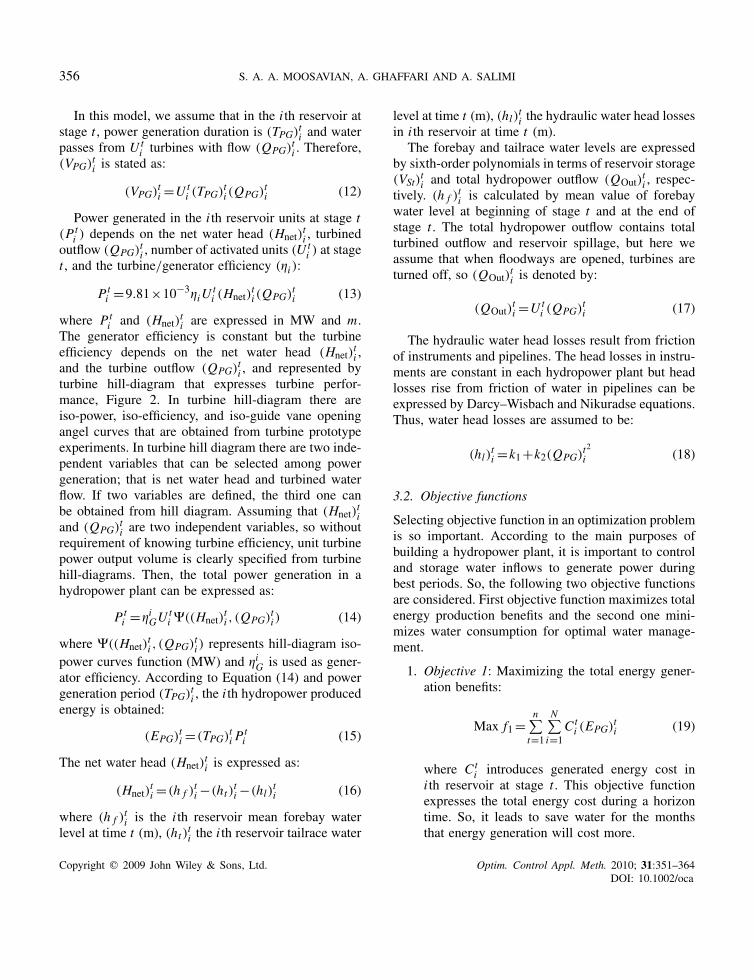
and the turbine outflow (QPG)ti , and represented byturbine hill-diagram that expresses turbine perfor-mance, Figure 2. In turbine hill-diagram there areiso-power, iso-efficiency, and iso-guide vane openingangel curves that are obtained from turbine prototypeexperiments. In turbine hill diagram there are two inde-pendent variables that can be selected among powergeneration; that is net water head and turbined waterflow. If two variables are defined, the third one canbe obtained from hill diagram. Assuming that (Hnet)

ti

and (QPG)ti are two independent variables, so withoutrequirement of knowing turbine efficiency, unit turbinepower output volume is clearly specified from turbinehill-diagrams. Then, the total power generation in ahydropower plant can be expressed as:

Pti =�iGU

ti �((Hnet)

ti , (QPG)ti ) (14)

where �((Hnet)ti , (QPG)ti ) represents hill-diagram iso-

power curves function (MW) and �iG is used as gener-ator efficiency. According to Equation (14) and powergeneration period (TPG)ti , the i th hydropower producedenergy is obtained:

(EPG)ti =(TPG)ti Pti (15)

The net water head (Hnet)ti is expressed as:

(Hnet)ti =(h f )

ti −(ht )

ti −(hl)

ti (16)

where (h f )ti is the i th reservoir mean forebay water

level at time t (m), (ht )ti the i th reservoir tailrace water

level at time t (m), (hl)ti the hydraulic water head lossesin i th reservoir at time t (m).

The forebay and tailrace water levels are expressedby sixth-order polynomials in terms of reservoir storage(VSt)ti and total hydropower outflow (QOut)

ti , respec-

tively. (h f )ti is calculated by mean value of forebay

water level at beginning of stage t and at the end ofstage t . The total hydropower outflow contains totalturbined outflow and reservoir spillage, but here weassume that when floodways are opened, turbines areturned off, so (QOut)

ti is denoted by:

(QOut)ti =Ut

i (QPG)ti (17)

The hydraulic water head losses result from frictionof instruments and pipelines. The head losses in instru-ments are constant in each hydropower plant but headlosses rise from friction of water in pipelines can beexpressed by Darcy–Wisbach and Nikuradse equations.Thus, water head losses are assumed to be:

(hl)ti =k1+k2(QPG)t

2

i (18)

3.2. Objective functions

Selecting objective function in an optimization problemis so important. According to the main purposes ofbuilding a hydropower plant, it is important to controland storage water inflows to generate power duringbest periods. So, the following two objective functionsare considered. First objective function maximizes totalenergy production benefits and the second one mini-mizes water consumption for optimal water manage-ment.

1. Objective 1: Maximizing the total energy gener-ation benefits:

Max f1=n∑

t=1

N∑i=1

Cti (EPG)ti (19)

where Cti introduces generated energy cost in

i th reservoir at stage t . This objective functionexpresses the total energy cost during a horizontime. So, it leads to save water for the monthsthat energy generation will cost more.

Copyright q 2009 John Wiley & Sons, Ltd. Optim. Control Appl. Meth. 2010; 31:351–364DOI: 10.1002/oca

SEQUENTIAL QUADRATIC PROGRAMMING AND ANALYTIC HIERARCHY PROCESS 357

Figure 2. Hill-diagram of Karoon 1 turbines.

2. Objective 2: Minimizing the mean specific waterconsumption:

Min f2= 1

nN

n∑t=1

N∑i=1

(VPG)ti

(EPG)ti(20)

The volume of turbined water that generates1MWh electrical energy is called specific waterconsumption (m3/MWh). This objective functionaims to generate more energy by using less waterduring a horizon time, so leads to optimal waterusage in producing more energy.

3.3. Constraints

The following five types of constraints are considered:

1. Volume of outflow water limitations:

(VOut)ti�(VRan)

ti +(Vu)

ti +

∑k∈U (i)

(VOut)tk (21)

The useful water equals to (Vu)ti=(VSt)ti −(VSt)min

i where (VSt)mini is the possible reservoir

storage. This constraint means that volume ofoutput water during a specified period should notcause decreasing water level to minimum turbineintake head.

Copyright q 2009 John Wiley & Sons, Ltd. Optim. Control Appl. Meth. 2010; 31:351–364DOI: 10.1002/oca

358 S. A. A. MOOSAVIAN, A. GHAFFARI AND A. SALIMI

2. Net head water level limitations:

(hnet)mini �(hnet)

ti�(hnet)

maxi (22)

According to turbine design concepts, net headwater is limited, so this limitation is consideredwith the inequality form of Equation (22).

3. Reservoir storage bounds:

(VSt)mini �(VSt)

ti�(VSt)

maxi (23)

Minimum water storage limit is the water volumethat can generate power at that forebay level andthe maximum storage volume is equal to themaximum reservoir capacity.

4. Turbine inflow limitations:

GLi ((Hnet)

ti )�(QPG)ti�GU

i ((Hnet)ti ) (24)

According to hill-diagram and normal operationzone, turbine inflow is limited but these limitationbounds vary with net head water. Thus GL

i andGU

i are turbine inflow lower and upper limitationfunctions that are obtained from hill-diagram.

5. Spillage limitations:

0�(VSp)ti�(VSp)

maxi (25)

where (VSp)maxi is determined from maximum

spillage flow (QSp)maxi and duration of time

interval. This constraint expresses that accordingto spillway structure, maximum volume of spilledwater at a specified time period is limited.

4. REAL AND SIMULATION RESULTS

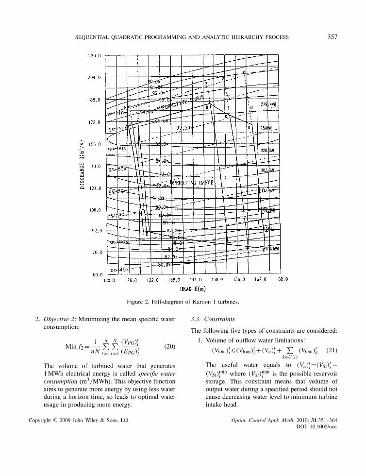
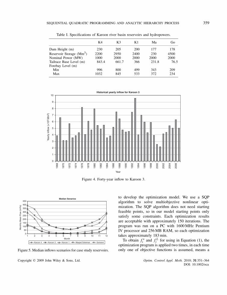
Karoon river basin, the largest basin in the Iran, isselected to implement the developed optimizationmethodology. The Karoon basin network consistsof five hydropower plants with nominal capacityof 8000 (MW). The system has four storage reser-voirs and one run-of-river plant. Figure 3 shows thereservoirs schematically and some specifications aredescribed in Table I.

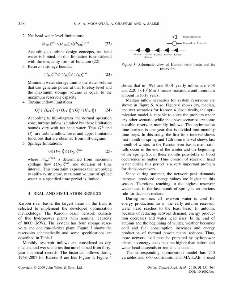
Monthly reservoir inflows are considered as dry,median, and wet scenarios that are obtained from forty-year historical records. The historical inflows during1968–2007 for Karoon 3 are like Figure 4. Figure 4

Karoon4Karoon1 Karoon3Masjed Soleima

Gotvan

Storage Reservoir

Run-of-River Reservoir

Figure 3. Schematic view of Karoon river basin and itsreservoirs.

shows that in 1993 and 2001 yearly inflow are 9.58and 2.20 (×103Mm3) means maximum and minimumamount in forty years.

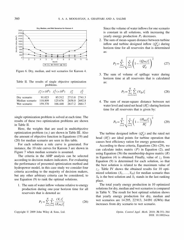
Median inflow scenarios for system reservoirs areshown in Figure 5. Also, Figure 6 shows dry, median,and wet scenarios for Karoon 4. Specifically, the opti-mization model is capable to solve the problem underany other scenario, while the above scenarios are somepossible reservoir monthly inflows. The optimizationtime horizon is one year that is divided into monthlytime steps. In this study, the first time interval showsfirst month of spring and 12th time interval shows lastmonth of winter. In the Karoon river basin, main rain-falls occur in the end of the winter and the beginningof the spring. So, in these months possibility of floodoccurrence is higher. Thus control of reservoir headwater during this period is a very important problemfor decision-makers.

Since during summer, the network peak demandsincrease, produced energy values are higher in thisseason. Therefore, reaching to the highest reservoirwater head in the last month of spring is an obviousrule for decision-makers.

During summer, all reservoir water is used forenergy production, so in the early autumn reservoirwater head reaches to the least head. In autumn,because of reducing network demand, energy produc-tion decreases and water head rises. In the end ofautumn and the beginning of winter, weather becomescold and fuel consumption increases and energyproduction of thermal power plants reduces. Thus,more network load must be prepared by hydropowerplants, so energy costs become higher than before andwater head descends or remains constant.

The corresponding optimization model has 240variables and 660 constraints, and MATLAB is used

Copyright q 2009 John Wiley & Sons, Ltd. Optim. Control Appl. Meth. 2010; 31:351–364DOI: 10.1002/oca

SEQUENTIAL QUADRATIC PROGRAMMING AND ANALYTIC HIERARCHY PROCESS 359

Table I. Specifications of Karoon river basin reservoirs and hydropowers.

K4 K3 K1 Ma Go

Dam Height (m) 230 205 200 177 178Reservoir Storage (Mm3) 2200 2950 2400 230 4500Nominal Power (MW) 1000 2000 2000 2000 2000Tailrace Base Level (m) 843.4 661.7 366 231.8 76.5Forebay Level (m)

Min 996 800 499 343 209Max 1032 845 533 372 234

Historical yearly inflow for Karoon 3

0

1

2

3

4

5

6

7

8

9

10

1968

1970

1972

1974

1976

1978

1980

1982

1984

1986

1988

1990

1992

1994

1996

1998

2000

2002

2004

2006

Year

Year

ly in

flow

(×

103

Mm

3 )

Figure 4. Forty-year inflow to Karoon 3.

Median Senarios

0

50

100

150

200

250

300

350

400

450

1Month

Mon

thly

Mea

n F

low

(m

3 /s)

Karoon 4 Karoon 3 Karoon 1 Masjed Soleiman Gotvand

2 3 4 5 6 7 8 9 10 11 12

Figure 5. Median inflows scenarios for case study reservoirs.

to develop the optimization model. We use a SQPalgorithm to solve multiobjective nonlinear opti-mization. The SQP algorithm does not need startingfeasible points, so in our model starting points onlysatisfy some constraints. Each optimization resultsare acceptable with approximately 150 iterations. Theprogram was run on a PC with 1600MHz PentiumIV processor and 256MB RAM, so each optimizationtakes approximately 183min.

To obtain f ∗i and f Li for using in Equation (1), the

optimization program is applied two times, in each timeonly one of objective functions is assumed, means a

Copyright q 2009 John Wiley & Sons, Ltd. Optim. Control Appl. Meth. 2010; 31:351–364DOI: 10.1002/oca

360 S. A. A. MOOSAVIAN, A. GHAFFARI AND A. SALIMI

Dry, Median, and Wet Senarios for Karoon 4

0

300

600

900

1200

1500

1800

2100

2400

2700

3000

Month

Mon

thly

Inflo

w (

Mm

3 )

Dry Median Wet

1 2 3 4 5 6 7 8 9 10 11 12

Figure 6. Dry, median, and wet scenarios for Karoon 4.

Table II. The results of single objective optimizationproblems.

f ∗1 (×106) f L1 (×106) f ∗

2 f L2

Dry scenario 91.023 85.512 2713.8 2741.3Median scenario 118.809 125.676 2658.0 2692.8Wet scenario 159.370 166.448 2617.2 2661.7

single optimization problem is solved at each time. Theresults of these two optimization problems are shownin Table II.

Here, the weights that are used in multiobjectiveoptimization problem (wi ) are shown in Table III. Alsothe amount of objective function in Equations (19) and(20) for median scenario are seen in this table.

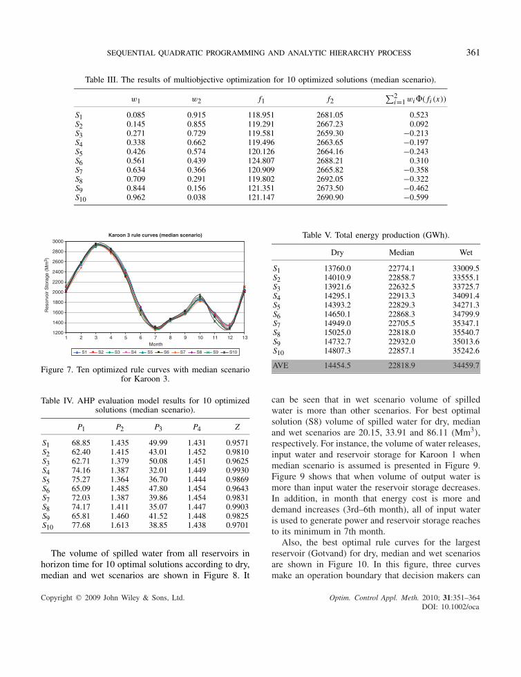
For each solution a rule curve is generated. Forinstance, the 10 rule curves for Karoon 3 are shown inFigure 7 when median scenario is assumed.

The criteria in the AHP analysis can be selectedaccording to decision makers indicators. For evaluatingthe performance of presented optimization method andhydropower model, in this case study we consider fourcriteria according to the majority of decision makers,but any other arbitrary criteria can be considered, touse Equation (9) to rank the optimal solutions.

1. The sum of water inflow volume relative to energyproduction during one-year horizon time for allreservoirs that is denoted as:

P1=N∑i=1

n∑t=1

(Vr )ti(EPG)ti

(26)

Since the volume of water inflows for one scenariois constant in all solutions, with increasing theyearly energy production P1 decreases.

2. The sum of mean-square distance between turbineinflow and turbine designed inflow (Qi

d) duringhorizon time for all reservoirs that is determinedas:

P2=N∑i=1

√√√√ n∑t=1

(1− (QPG)ti

Qid

)2

(27)

3. The sum of volume of spillage water duringhorizon time at all reservoirs that is calculatedas:

P3=N∑i=1

n∑t=1

(VSp)ti (28)

4. The sum of mean-square distance between netwater level and rated net head (Hi

r ) during horizontime for all reservoirs that is given by:

P4=N∑i=1

√√√√ n∑t=1

(1− (Hnet)

ti

H ir

)2

(29)

The turbine designed inflow (Qid) and the rated net

head (Hir ) are ideal points for turbine operation that

causes best efficiency ration for energy generation.According to these criteria, Equations (26)–(29), we

can calculate index matrix (P) in Equation (2), andusing Equation (3b) the membership degree matrix (R)

in Equation (4) is obtained. Finally, value of z j fromEquation (9) is determined for each solution, so thatthe best solution is related to the maximum value ofz j . Table IV shows the obtained results for 10 opti-mized solutions (S1, . . . , S10) for median scenario thusS4 is the best solution and S1 stands in the last rankingplace.

The total yearly energy production in 10 optimizedsolutions for dry, median and wet scenarios is comparedin Table V. The result for best optimal solution showsthat yearly energy production for dry, median andwet scenarios are 14 295, 22 913, 34 091 (GWh) thatincreases from dry scenario to wet scenario.

Copyright q 2009 John Wiley & Sons, Ltd. Optim. Control Appl. Meth. 2010; 31:351–364DOI: 10.1002/oca

SEQUENTIAL QUADRATIC PROGRAMMING AND ANALYTIC HIERARCHY PROCESS 361

Table III. The results of multiobjective optimization for 10 optimized solutions (median scenario).

w1 w2 f1 f2∑2

i=1wi�( fi (x))

S1 0.085 0.915 118.951 2681.05 0.523S2 0.145 0.855 119.291 2667.23 0.092S3 0.271 0.729 119.581 2659.30 −0.213S4 0.338 0.662 119.496 2663.65 −0.197S5 0.426 0.574 120.126 2664.16 −0.243S6 0.561 0.439 124.807 2688.21 0.310S7 0.634 0.366 120.909 2665.82 −0.358S8 0.709 0.291 119.802 2692.05 −0.322S9 0.844 0.156 121.351 2673.50 −0.462S10 0.962 0.038 121.147 2690.90 −0.599

Karoon 3 rule curves (median scenario)

1200

1400

1600

1800

2000

2200

2400

2600

2800

3000

Month

Res

orvo

ir S

tora

ge (

Mm

3 )

S1 S2 S3 S4 S5 S6 S7 S8 S9 S10

1 2 3 4 5 6 7 8 9 10 11 12 13

Figure 7. Ten optimized rule curves with median scenariofor Karoon 3.

Table IV. AHP evaluation model results for 10 optimizedsolutions (median scenario).

P1 P2 P3 P4 Z

S1 68.85 1.435 49.99 1.431 0.9571S2 62.40 1.415 43.01 1.452 0.9810S3 62.71 1.379 50.08 1.451 0.9625S4 74.16 1.387 32.01 1.449 0.9930S5 75.27 1.364 36.70 1.444 0.9869S6 65.09 1.485 47.80 1.454 0.9643S7 72.03 1.387 39.86 1.454 0.9831S8 74.17 1.411 35.07 1.447 0.9903S9 65.81 1.460 41.52 1.448 0.9825S10 77.68 1.613 38.85 1.438 0.9701

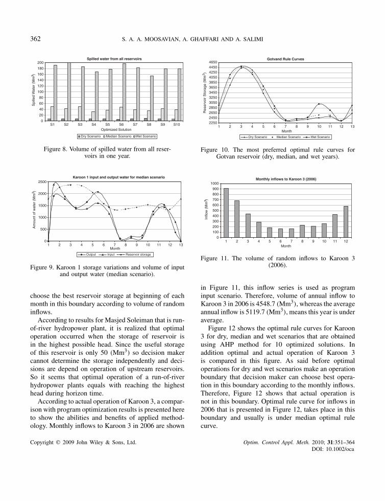
The volume of spilled water from all reservoirs inhorizon time for 10 optimal solutions according to dry,median and wet scenarios are shown in Figure 8. It

Table V. Total energy production (GWh).

Dry Median Wet

S1 13760.0 22774.1 33009.5S2 14010.9 22858.7 33555.1S3 13921.6 22632.5 33725.7S4 14295.1 22913.3 34091.4S5 14393.2 22829.3 34271.3S6 14650.1 22868.3 34799.9S7 14949.0 22705.5 35347.1S8 15025.0 22818.0 35540.7S9 14732.7 22932.0 35013.6S10 14807.3 22857.1 35242.6

AVE 14454.5 22818.9 34459.7

can be seen that in wet scenario volume of spilledwater is more than other scenarios. For best optimalsolution (S8) volume of spilled water for dry, medianand wet scenarios are 20.15, 33.91 and 86.11 (Mm3),respectively. For instance, the volume of water releases,input water and reservoir storage for Karoon 1 whenmedian scenario is assumed is presented in Figure 9.Figure 9 shows that when volume of output water ismore than input water the reservoir storage decreases.In addition, in month that energy cost is more anddemand increases (3rd–6th month), all of input wateris used to generate power and reservoir storage reachesto its minimum in 7th month.

Also, the best optimal rule curves for the largestreservoir (Gotvand) for dry, median and wet scenariosare shown in Figure 10. In this figure, three curvesmake an operation boundary that decision makers can

Copyright q 2009 John Wiley & Sons, Ltd. Optim. Control Appl. Meth. 2010; 31:351–364DOI: 10.1002/oca

362 S. A. A. MOOSAVIAN, A. GHAFFARI AND A. SALIMI

Spilled water from all reservoirs

0

20

40

60

80

100

120

140

160

180

200

Optimized Solution

Spi

lled

Wat

er (

Mm

3 )

Dry Scenario Median Scenario Wet Scenario

S1 S2 S3 S4 S5 S6 S7 S8 S9 S10

Figure 8. Volume of spilled water from all reser-voirs in one year.

Karoon 1 input and output water for median scenario

0

500

1000

1500

2000

2500

Month

Am

ount

of w

ater

(M

m3 )

Output Input Reservoir storage

1 2 3 4 5 6 7 8 9 10 11 12 13

Figure 9. Karoon 1 storage variations and volume of inputand output water (median scenario).

choose the best reservoir storage at beginning of eachmonth in this boundary according to volume of randominflows.

According to results for Masjed Soleiman that is run-of-river hydropower plant, it is realized that optimaloperation occurred when the storage of reservoir isin the highest possible head. Since the useful storageof this reservoir is only 50 (Mm3) so decision makercannot determine the storage independently and deci-sions are depend on operation of upstream reservoirs.So it seems that optimal operation of a run-of-riverhydropower plants equals with reaching the highesthead during horizon time.

According to actual operation of Karoon 3, a compar-ison with program optimization results is presented hereto show the abilities and benefits of applied method-ology. Monthly inflows to Karoon 3 in 2006 are shown

Gotvand Rule Curves

2250245026502850305032503450365038504050425044504650

Month

Res

ervo

ir S

tora

ge (

Mm

3 )

Dry Scenario Median Scenario Wet Scenario

1 2 3 4 5 6 7 8 9 10 11 12 13

Figure 10. The most preferred optimal rule curves forGotvan reservoir (dry, median, and wet years).

Monthly inflows to Karoon 3 (2006)

0

100

200

300

400

500

600

700

800

900

1000

Month

Inflo

w (

Mm

3 )

1 2 3 4 5 6 7 8 9 10 11 12

Figure 11. The volume of random inflows to Karoon 3(2006).

in Figure 11, this inflow series is used as programinput scenario. Therefore, volume of annual inflow toKaroon 3 in 2006 is 4548.7 (Mm3), whereas the averageannual inflow is 5119.7 (Mm3), means this year is underaverage.

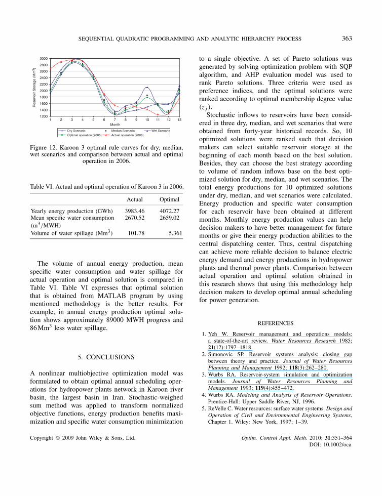
Figure 12 shows the optimal rule curves for Karoon3 for dry, median and wet scenarios that are obtainedusing AHP method for 10 optimized solutions. Inaddition optimal and actual operation of Karoon 3is compared in this figure. As said before optimaloperations for dry and wet scenarios make an operationboundary that decision maker can choose best opera-tion in this boundary according to the monthly inflows.Therefore, Figure 12 shows that actual operation isnot in this boundary. Optimal rule curve for inflows in2006 that is presented in Figure 12, takes place in thisboundary and usually is under median optimal rulecurve.

Copyright q 2009 John Wiley & Sons, Ltd. Optim. Control Appl. Meth. 2010; 31:351–364DOI: 10.1002/oca

SEQUENTIAL QUADRATIC PROGRAMMING AND ANALYTIC HIERARCHY PROCESS 363

1200

1400

1600

1800

2000

2200

2400

2600

2800

3000

Month

Res

ervo

ir S

tora

ge (

Mm

3 )

Dry Scenario Median Scenario Wet ScenarioOptimal operation (2006) Actual operation (2006)

1 2 3 4 5 6 7 8 9 10 11 12 13

Figure 12. Karoon 3 optimal rule curves for dry, median,wet scenarios and comparison between actual and optimal

operation in 2006.

Table VI. Actual and optimal operation of Karoon 3 in 2006.

Actual Optimal

Yearly energy production (GWh) 3983.46 4072.27Mean specific water consumption 2670.52 2659.02(m3/MWH)

Volume of water spillage (Mm3) 101.78 5.361

The volume of annual energy production, meanspecific water consumption and water spillage foractual operation and optimal solution is compared inTable VI. Table VI expresses that optimal solutionthat is obtained from MATLAB program by usingmentioned methodology is the better results. Forexample, in annual energy production optimal solu-tion shows approximately 89000 MWH progress and86Mm3 less water spillage.

5. CONCLUSIONS

A nonlinear multiobjective optimization model wasformulated to obtain optimal annual scheduling oper-ations for hydropower plants network in Karoon riverbasin, the largest basin in Iran. Stochastic-weighedsum method was applied to transform normalizedobjective functions, energy production benefits maxi-mization and specific water consumption minimization

to a single objective. A set of Pareto solutions wasgenerated by solving optimization problem with SQPalgorithm, and AHP evaluation model was used torank Pareto solutions. Three criteria were used aspreference indices, and the optimal solutions wereranked according to optimal membership degree value(z j ).

Stochastic inflows to reservoirs have been consid-ered in three dry, median, and wet scenarios that wereobtained from forty-year historical records. So, 10optimized solutions were ranked such that decisionmakers can select suitable reservoir storage at thebeginning of each month based on the best solution.Besides, they can choose the best strategy accordingto volume of random inflows base on the best opti-mized solution for dry, median, and wet scenarios. Thetotal energy productions for 10 optimized solutionsunder dry, median, and wet scenarios were calculated.Energy production and specific water consumptionfor each reservoir have been obtained at differentmonths. Monthly energy production values can helpdecision makers to have better management for futuremonths or give their energy production abilities to thecentral dispatching center. Thus, central dispatchingcan achieve more reliable decision to balance electricenergy demand and energy productions in hydropowerplants and thermal power plants. Comparison betweenactual operation and optimal solution obtained inthis research shows that using this methodology helpdecision makers to develop optimal annual schedulingfor power generation.

REFERENCES

1. Yeh W. Reservoir management and operations models:a state-of-the-art review. Water Resources Research 1985;21(12):1797–1818.

2. Simonovic SP. Reservoir systems analysis: closing gapbetween theory and practice. Journal of Water ResourcesPlanning and Management 1992; 118(3):262–280.

3. Wurbs RA. Reservoir-system simulation and optimizationmodels. Journal of Water Resources Planning andManagement 1993; 119(4):455–472.

4. Wurbs RA. Modeling and Analysis of Reservoir Operations.Prentice-Hall: Upper Saddle River, NJ, 1996.

5. ReVelle C. Water resources: surface water systems. Design andOperation of Civil and Environmental Engineering Systems,Chapter 1. Wiley: New York, 1997; 1–39.

Copyright q 2009 John Wiley & Sons, Ltd. Optim. Control Appl. Meth. 2010; 31:351–364DOI: 10.1002/oca

364 S. A. A. MOOSAVIAN, A. GHAFFARI AND A. SALIMI

6. Momoh JA, El-Hawary ME, Adapa R. A review of selectedoptimal power flow literature to 1993, part II: Newton, linearprogramming and interior point methods. IEEE Transactionson Systems 1999; 14(1):105–111.

7. Djordjevic B. Cybernetics in Water Resources Management.Water Resources Publications: Highlands, Ranch, CO, U.S.A.,1993.

8. Burke EK, Landa Silva JD. The influence of the fitnessevaluation method on the performance of multiobjective searchalgorithms. European Journal of Operational Research 2006;169:875–897.

9. Khu ST, Madsen H. Multiobjective calibration withPareto preference ordering: an application to rainfall-runoff model calibration. Water Resources Research 2005;41(3):1–14. DOI: 10.1029/2004WR003041.

10. Keeney R, Raiffa H. Decisions with Multiple Objectives—Preferences and Value Tradeoffs. Wiley: New York, U.S.A.,1976.

11. Lin JG. Multiple-objective problems: Pareto-optimal solutionsby method of proper equality constraints. IEEE Transactionson Automatic Control 1976; AC-21(5):641–650.

12. Guariso G, Rinaldi S, Soncini-Sessa R. The managementof Lake Como: a multiobjective analysis. Water ResourcesResearch 1986; 22(2):109–120.

13. Liong SY, Tariq AA, Lee KS. Application of evolutionaryalgorithm in reservoir operations. Journal of the Institution ofEngineers, Singapore 2004; 44(1):39–54.

14. Hwang CL, Masud AS. Multiple Objective Decision Making-Methods and Applications: A Stateof-the-Art Survey. LectureNotes in Economics and Mathematical Systems, vol. 164.Springer: Berlin, 1979.

15. Steuer R. Multiple Criteria Optimization: Theory,Computation and Application. Wiley: New York, 1986.

16. Keeney R, Raiffa H. Decisions with Multiple Objectives—Preferences and Value Tradeoffs. Wiley: New York, 1976.

17. Kim JB, Wallace D. A goal-oriented design evaluationmodel. ASME Design Theory and Methodology Conference.Sacramento: CA, U.S.A., 1997.

18. Wallace DR, Jakiela MJ, Flowers WC. Multiple criteriaoptimization under probabilistic design specifications usinggenetic algorithms. Computer Aided Design 1996; 28:405–421.

19. Tamiz M, Jones D, Romero C. Goal programming for decisionmaking: an overview of the current state-of-the-art. EuropeanJournal of Operational Research 1998; 111:569–581.

20. Charnes A, Cooper WW, Ferguson RO. Optimal estimation ofexecutive compensation by linear programming. ManagementScience 1955; 1:138–151.

21. Charnes A, Cooper WW. Management Models and IndustrialApplications of Linear Programming. Wiley: New York, 1961.

22. Andersson J. A survey of multiobjective optimization inengineering design. Technical Report LiTH-IKP-R-1097,Department of Mechanical Engineering, Linkoping University,Linkoping, Sweden, 2000.

23. Krus P, Palmberg JO, Lohr F, Backlund G. The impactof computational performance on optimisation in aircraftdesign. I MECH E, AEROTECH 95, Birmingham, U.K.,1995.

24. Chiampi M, Ragusa C, Repetto M. Fuzzy approach formultiobjective optimization in magnetics. IEEE Transactionson Magnetics 1996; 32:1234–1237.

25. Chiampi M. Multiobjective optimization with stochasticalgorithms and fuzzy definition of objective function.International Journal of Applied Electromagnetics inMaterials 1998; 9:381–389.

26. Zimmermann HJ. Intelligent system design support by fuzzymulticriteria decision making and/or evolutionary algorithms.IEEE International Conference on Fuzzy Systems, Yokohama,Japan, 1995.

27. Murata T, Ishibuchi H. Multiobjective genetic algorithm andits application to flow-shop scheduling. International Journalof Computers and Engineering 1996; 30(4):957–968.

28. Murata T, Ishibuchi H, Gen M. Specification of geneticsearch directions in cellular multiobjective genetic algorithms.Proceedings of First International Conference on EvolutionaryMulti-Criterion Optimization. Springer: Berlin, 2001;82–95.

29. Jin Y, Okabe T, Sendhoff B. Adapting weighted aggregationfor multiobjective evolution strategies. Proceedings of FirstInternational Conference on Evolutionary Multi-CriterionOptimization, Zurich, Switzerland, 2001.

30. Saaty TL. The Analytical Hierarchy Process, Planning,Priority, Resource Allocation. RWS Publications: U.S.A.,1980.

31. Saaty TL. Axiomatic foundation of the analytic hierarchyprocess. Management Science 1986; 32(7):841–855.

32. Saaty TL. Decision Making for Leaders. RWS Publications:Pittsburgh, U.S.A., 1992.

33. Chen SY. Advanced Water Resources Fuzzy Set Theory andApplication. Jilin University Press: Jilin, 2002.

Copyright q 2009 John Wiley & Sons, Ltd. Optim. Control Appl. Meth. 2010; 31:351–364DOI: 10.1002/oca