Noncommutative symmetric functions

arX

iv:h

ep-t

h/94

0712

4v1

20

Jul 1

994

NONCOMMUTATIVE SYMMETRIC FUNCTIONS

I.M. Gelfand, D. Krob, A. Lascoux,

B. Leclerc, V.S. Retakh and J.-Y. Thibon

http://arXiv.org/abs/hep-th/9407124v1

Israel M. GelfandDepartment of MathematicsRutgers UniversityNew Brunswick, N.J. 08903U.S.A.

Daniel KrobLaboratoire d’Informatique Theorique et ProgrammationUniversite Paris 72, place Jussieu75251 Paris cedex 05France

Alain LascouxLaboratoire d’Informatique Theorique et ProgrammationUniversite Paris 72, place Jussieu75251 Paris cedex 05France

Bernard LeclercLaboratoire d’Informatique Theorique et ProgrammationUniversite Paris 72, place Jussieu75251 Paris cedex 05France

Vladimir S. RetakhDIMACSRutgers UniversityNew Brunswick, N.J. 08903U.S.A.

Jean-Yves ThibonInstitut Gaspard MongeUniversite de Marne-la-Vallee2, rue de la Butte-Verte93166 Noisy-le-Grand cedexFrance

Contents

1 Introduction 3

2 Background 6

2.1 Outline of the commutative theory . . . . . . . . . . . . . . . . . . . . . . . . . . 62.2 Quasi-determinants . . . . . . . . . . . . . . . . . . . . . . . . . . . . . . . . . . . 8

3 Formal noncommutative symmetric functions 14

3.1 Elementary, complete and power sums functions . . . . . . . . . . . . . . . . . . 143.2 Ribbon Schur functions . . . . . . . . . . . . . . . . . . . . . . . . . . . . . . . . 203.3 Quasi-Schur functions . . . . . . . . . . . . . . . . . . . . . . . . . . . . . . . . . 22

4 Transition matrices 26

4.1 S and Λ . . . . . . . . . . . . . . . . . . . . . . . . . . . . . . . . . . . . . . . . . 274.2 S and Ψ . . . . . . . . . . . . . . . . . . . . . . . . . . . . . . . . . . . . . . . . . 284.3 S and Φ . . . . . . . . . . . . . . . . . . . . . . . . . . . . . . . . . . . . . . . . . 294.4 S and R . . . . . . . . . . . . . . . . . . . . . . . . . . . . . . . . . . . . . . . . . 314.5 Λ and Ψ . . . . . . . . . . . . . . . . . . . . . . . . . . . . . . . . . . . . . . . . . 324.6 Λ and Φ . . . . . . . . . . . . . . . . . . . . . . . . . . . . . . . . . . . . . . . . . 334.7 Λ and R . . . . . . . . . . . . . . . . . . . . . . . . . . . . . . . . . . . . . . . . . 334.8 Ψ and R . . . . . . . . . . . . . . . . . . . . . . . . . . . . . . . . . . . . . . . . . 344.9 Φ and R . . . . . . . . . . . . . . . . . . . . . . . . . . . . . . . . . . . . . . . . . 374.10 Φ and Ψ . . . . . . . . . . . . . . . . . . . . . . . . . . . . . . . . . . . . . . . . . 39

5 Connections with Solomon’s descent algebra 43

5.1 Internal product . . . . . . . . . . . . . . . . . . . . . . . . . . . . . . . . . . . . 435.2 Lie idempotents . . . . . . . . . . . . . . . . . . . . . . . . . . . . . . . . . . . . . 475.3 Eulerian idempotents . . . . . . . . . . . . . . . . . . . . . . . . . . . . . . . . . . 535.4 Eulerian symmetric functions . . . . . . . . . . . . . . . . . . . . . . . . . . . . . 55

5.4.1 Noncommutative Eulerian polynomials . . . . . . . . . . . . . . . . . . . . 555.4.2 Noncommutative trigonometric functions . . . . . . . . . . . . . . . . . . 58

5.5 Continuous Baker-Campbell-Hausdorff formulas . . . . . . . . . . . . . . . . . . . 60

6 Duality 64

6.1 Quasi-symmetric functions . . . . . . . . . . . . . . . . . . . . . . . . . . . . . . . 646.2 The pairing between Sym and Qsym . . . . . . . . . . . . . . . . . . . . . . . . . 65

7 Specializations 67

7.1 Rational symmetric functions of n noncommutative variables . . . . . . . . . . . 677.2 Rational (s, d)-symmetric functions of n noncommutative variables . . . . . . . . 707.3 Polynomial symmetric functions of n noncommutative variables . . . . . . . . . . 737.4 Symmetric functions associated with a matrix . . . . . . . . . . . . . . . . . . . . 767.5 Noncommutative symmetric functions and the center of U(gln) . . . . . . . . . . 787.6 Twisted symmetric functions . . . . . . . . . . . . . . . . . . . . . . . . . . . . . 82

8 Noncommutative rational power series 84

8.1 Noncommutative continued S-fractions . . . . . . . . . . . . . . . . . . . . . . . . 848.2 Noncommutative Pade approximants . . . . . . . . . . . . . . . . . . . . . . . . . 898.3 Noncommutative orthogonal polynomials . . . . . . . . . . . . . . . . . . . . . . 908.4 Noncommutative continued J-fractions . . . . . . . . . . . . . . . . . . . . . . . . 92

1

8.5 Rational power series and Hankel matrices . . . . . . . . . . . . . . . . . . . . . . 948.6 The characteristic polynomial of the generic matrix, and a noncommutative Cayley-

Hamilton theorem . . . . . . . . . . . . . . . . . . . . . . . . . . . . . . . . . . . 96

9 Appendix : automata and matrices over noncommutative rings 101

2

1 Introduction

A large part of the classical theory of symmetric functions is fairly independent of theirinterpretation as polynomials in some underlying set of variables X. In fact, if X is sup-posed infinite, the elementary symmetric functions Λk(X) are algebraically independent,and what one really considers is just a polynomial algebra K[Λ1,Λ2, . . .], graded by theweight function w(Λk) = k instead of the usual degree d(Λk) = 1.

Such a construction still makes sense when the Λk are interpreted as noncommutingindeterminates and one can try to lift to the free associative algebra Sym = K〈Λ1,Λ2, . . .〉the expressions of the other classical symmetric functions in terms of the elementary ones,in order to define their noncommutative analogs (Section 3.1). Several algebraic and lin-ear bases are obtained in this way, including two families of “power-sums”, correspondingto two different noncommutative analogs of the logarithmic derivative of a power series.Moreover, most of the determinantal relations of the classical theory remain valid, pro-vided that determinants be replaced by quasi-determinants (cf. [GR1], [GR2] or [KL]).

In the commutative theory, Schur functions constitute the fundamental linear basisof the space of symmetric functions. In the noncommutative case, it is possible to definea convenient notion of quasi-Schur function (for any skew Young diagram) using quasi-determinants, however most of these functions are not polynomials in the generators Λk,but elements of the skew field generated by the Λk. The only quasi-Schur functions whichremain polynomials in the generators are those which are indexed by ribbon shapes (alsocalled skew hooks) (Section 3.2).

A convenient property of these noncommutative ribbon Schur functions is that theyform a linear basis of Sym. More importantly, perhaps, they also suggest some kind ofnoncommutative analog of the fundamental relationship between the commutative theoryof symmetric functions and the representation theory of the symmetric group. The roleof the character ring of the symmetric group is here played by a certain subalgebra Σn ofits group algebra. This is the descent algebra, whose discovery is due to L. Solomon (cf.[So2]). There is a close connection, which has been known from the beginning, betweenthe product of the descent algebra, and the Kronecker product of representations of thesymmetric group. The fact that the homogeneous components of Sym have the samedimensions as the corresponding descent algebras allows us to transport the product ofthe descent algebras, thus defining an analog of the usual internal product of symmetricfunctions (Section 5).

Several Hopf algebra structures are classically defined on (commutative or not) polyno-mial algebras. One possibility is to require that the generators form an infinite sequenceof divided powers. For commutative symmetric functions, this is the usual structure,which is precisely compatible with the internal product. The same is true in the noncom-mutative setting, and the natural Hopf algebra structure of noncommutative symmetricfunctions provides an efficient tool for computing in the descent algebra. This illustratesonce more the importance of Hopf algebras in Combinatorics, as advocated by Rota andhis school (see e.g. [JR]).

This can be explained by an interesting realization of noncommutative symmetricfunctions, as a certain subalgebra of the convolution algebra of a free associative algebra(interpreted as a Hopf algebra in an appropriate way). This algebra is discussed at lengthin the recent book [Re] by C. Reutenauer, where one finds many interesting results which

3

can be immediately translated in the language of noncommutative symmetric functions.We illustrate this correspondence on several examples. In particular, we show that theLie idempotents in the descent algebra admit a simple interpretation in terms of non-commutative symmetric functions. We also discuss a certain recently discovered family ofidempotents of Σn (the Eulerian idempotents), which arise quite naturally in the contextof noncommutative symmetric functions, and explain to a large extent the combinatoricsof Eulerian polynomials. All these considerations are strongly related to the combina-torics of the Hausdorff series, more precisely of its continous analog, which expresses thelogarithm of the solution of a noncommutative linear differential equation as a series ofiterated integrals (cf. [Mag][C2][BMP]). The theory of such series has been initiatedand widely developed by K. T. Chen in his work on homotopy theory (cf. [C3][C4]),starting from his fundamental observation that paths on a manifold can be convenientlyrepresented by noncommutative power series [C1].

The algebra of commutative symmetric functions has a canonical scalar product, forwhich it is self-dual as a Hopf algebra. In the noncommutative theory, the algebra ofsymmetric functions differs from its dual, which, as shown in [MvR], can be identifiedwith the algebra of quasi-symmetric functions (Section 6).

Another classical subject in the commutative theory is the description of the transitionmatrices between the various natural bases. This question is considered in Section 4.It is worth noting that the rigidity of the noncommutative theory leads to an explicitdescription of most of these matrices.

We also investigate the general quasi-Schur functions. As demonstrated in [GR1] or[GR2], the natural object replacing the determinant in noncommutative linear algebra isthe quasi-determinant, which is an analog of the ratio of two determinants. Similarly,Schur functions will be replaced by quasi-Schur functions, which are analogs of the ratioof two ordinary Schur functions. The various determinantal expressions of the classicalSchur functions can then be adapted to quasi-Schur functions (Section 3.3). This provesuseful, for example, when dealing with noncommutative continued fractions and orthog-onal polynomials. Indeed, the coefficients of the S-fraction or J-fraction expansions ofa noncommutative formal power series are quasi-Schur functions of a special type, aswell as the coefficients of the typical three-term recurrence relation for noncommutativeorthogonal polynomials.

A rich field of applications of the classical theory is provided by specializations. Aspointed out by Littlewood, since the elementary functions are algebraically independent,the process of specialization is not restricted to the underlying variables xi, but can becarried out directly at the level of the Λk, which can then be specialized in a totally arbi-trary way, and can still be formally considered as symmetric functions of some fictitiousset of arguments. The same point of view can be adopted in the noncommutative case,and we discuss several important examples of such specializations (Section 7). The mostnatural question is whether the formal symmetric functions can actually be interpretedas functions of some set of noncommuting variables. Several answers can be proposed.

In Section 7.1, we take as generating function λ(t) =∑

k Λk tk of the elementary sym-

metric functions a quasi-determinant of the Vandermonde matrix in the noncommutativeindeterminates x1, x2, . . . , xn and x = t−1. This is a monic left polynomial of degree nin x, which is annihilated by the substitution x = xi for every i = 1, . . . n. Therefore theso-defined functions are noncommutative analogs of the ordinary symmetric functions of n

4

commutative variables. They are actually symmetric in the usual sense. These functionsare no longer polynomials but rational functions of the xi. We show that they can beexpressed in terms of ratios of quasi-minors of the Vandermonde matrix, as in the classicalcase. We also indicate in Section 7.2 how to generalize these ideas in the context of skewpolynomial algebras.

In Section 7.3, we introduce another natural specialization, namely

λ(t) =←−−−∏

1≤k≤n

(1 + txk) = (1 + txn)(1 + txn−1)(1 + txn−2) · · · (1 + tx1) .

This leads to noncommutative polynomials which are symmetric for a special action ofthe symmetric group on the free associative algebra.

In Section 7.4, we take λ(t) to be a quasi-determinant of I + tA, where A = (aij) isa matrix with noncommutative entries, and I is the unit matrix. In this case, the usualfamilies of symmetric functions are polynomials in the aij with integer coefficients, andadmit a simple combinatorial description in terms of paths in the complete oriented graphlabelled by the entries of A. An interesting example, investigated in Section 7.5, is whenA = En = (eij), the matrix whose entries are the generators of the universal envelopingalgebra U(gln). We obtain a description of the center of U(gln) by means of the symmetricfunctions associated with the matrices E1, E2 − I, . . . , En − (n − 1)I. We also relatethese functions to Gelfand-Zetlin bases.

Finally, in Section 7.6, other kinds of specializations in skew polynomial algebras areconsidered.

The last section deals with some applications of quasi-Schur functions to the studyof rational power series with coefficients in a skew field, and to some related points ofnoncommutative linear algebra. We first discuss noncommutative continued fractions, or-thogonal polynomials and Pade approximants. The results hereby found are then appliedto rational power series in one variable over a skew field. One obtains in particular anoncommutative extension of the classical rationality criterion in terms of Hankel deter-minants (Section 8.5).

The n series λ(t) associated with the generic matrix of order n (defined in Section 7.4)are examples of rational series. Their denominators appear as n pseudo-characteristicpolynomials, for which a version of the Cayley-Hamilton theorem can be established(Section 8.6). In particular, the generic matrix posesses n pseudo-determinants, whichare true noncommutative analogs of the determinant. These pseudo-determinants reducein the case of U(gln) to the Capelli determinant, and in the case of the quantum groupGLq(n), to the quantum determinant (up to a power of q).

The theory of noncommutative rational power series has been initiated by M.P. Schut-zenberger, in relation with problems in formal languages and automata theory [Sc]. Thispoint of view is briefly discussed in an Appendix.

The authors are grateful to C. Reutenauer for interesting discussions at various stagesof the preparation of this paper.

5

2 Background

2.1 Outline of the commutative theory

Here is a brief review of the classical theory of symmetric functions. A standard referenceis Macdonald’s book [McD]. The notations used here are those of [LS1].

Denote by X = x1, x2, . . . an infinite set of commutative indeterminates, whichwill be called a (commutative) alphabet. The elementary symmetric functions Λk(X) arethen defined by means of the generating series

λ(X, t) :=∑

k≥0

tk Λk(X) =∏

i≥1

(1 + xit) . (1)

The complete homogeneous symmetric functions Sk(X) are defined by

σ(X, t) :=∑

k≥0

tk Sk(X) =∏

i≥1

(1− xit)−1 , (2)

so that the following fundamental relation holds

σ(X, t) = λ(X,−t)−1 . (3)

The power sums symmetric functions ψk(X) are defined by

ψ(X, t) :=∑

k≥1

tk−1 ψk(X) =∑

i≥1

xi (1− xit)−1 . (4)

These generating series satisfy the following relations

ψ(X, t) =d

dtlog σ(X, t) = −

d

dtlog λ(X,−t) , (5)

d

dtσ(X, t) = σ(X, t) ψ(X, t) , (6)

−d

dtλ(X,−t) = ψ(X, t) λ(X,−t) . (7)

Formula (7) is known as Newton’s formula. The so-called fundamental theorem ofthe theory of symmetric functions states that the Λk(X) are algebraically independent.Therefore, any formal power series f(t) = 1 +

∑k≥1 ak t

k may be considered as the spe-cialization of the series λ(X, t) to a virtual set of arguments A. The other families ofsymmetric functions associated to f(t) are then defined by relations (3) and (5). Thispoint of view was introduced by Littlewood and extensively developped in [Li1]. Forexample, the specialization Sn = 1/n! transforms the generating series σ(X, t) into theexponential function et. Thus, considering σ(X, t) as a symmetric analog of et, one canconstruct symmetric analogs for several related functions, such as trigonometric functions,Eulerian polynomials or Bessel polynomials. This point of view allows to identify theircoefficients as the dimensions of certain representations of the symmetric group [F1][F2].Also, any function admitting a symmetric analog can be given a q-analog, for example bymeans of the specialization X = 1, q, q2, . . . .

6

We denote by Sym the algebra of symmetric functions, i.e. the algebra generated overQ by the elementary functions. It is a graded algebra for the weight function w(Λk) = k,and the dimension of its homogeneous component of weight n, denoted by Symn, is equalto p(n), the number of partitions of n. A partition is a finite non-decreasing sequence ofpositive integers, I = (i1 ≤ i2 ≤ . . . ≤ ir). We shall also write I = (1α1 2α2 . . .), αm beingthe number of parts ik which are equal to m. The weight of I is |I| =

∑k ik and its length

is its number of (nonzero) parts ℓ(I) = r.

For a partition I, we set

ψI = ψα11 ψα2

2 · · · , ΛI = Λα11 Λα2

2 · · · , SI = Sα1

1 Sα22 · · · .

For I ∈ Zr, not necessarily a partition, the Schur function SI is defined by

SI = det (Sik+k−h)1≤h,k≤r (8)

where Sj = 0 for j < 0. The Schur functions indexed by partitions form a Z-basis of Sym,and one usually endows Sym with a scalar product (·, ·) for which this basis is orthonormal.The ψI form then an orthogonal Q-basis of Sym, with (ψI , ψI) = 1α1 α1! 2

α2 α2! · · · Thus,for a partition I of weigth n, n!/(ψI , ψI) is the cardinality of the conjugacy class of Sn

whose elements have αk cycles of length k for all k ∈ [1, n]. A permutation σ in this classwill be said of type I, and we shall write T (σ) = I.

These definitions are motivated by the following classical results of Frobenius. LetCF (Sn) be the ring of central functions of the symmetric group Sn. The Frobeniuscharacteristic map F : CF (Sn) −→ Symn associates with any central function ξ thesymmetric function

F(ξ) =1

n!

∑

σ∈Sn

ξ(σ) ψT (σ) =∑

|I|=n

ξ(I)ψI

(ψI , ψI)

where ξ(I) is the common value of the ξ(σ) for all σ such that T (σ) = I. We can alsoconsider F as a map from the representation ring R(Sn) to Symn by setting F([ρ]) =F(χρ), where [ρ] denotes the equivalence class of a representation ρ (we use the sameletter F for the two maps since this does not lead to ambiguities). Glueing these mapstogether, one has a linear map

F : R :=⊕

n≥0

R(Sn) −→ Sym ,

which turns out to be an isomorphism of graded rings (see for instance [McD] or [Zel]).We denote by [I] the class of the irreducible representation of Sn associated with thepartition I, and by χI its character. We have then F(χI) = SI (see e.g. [McD] p. 62).

The product ∗, defined on the homogeneous component Symn by

F([ρ]⊗ [η]) = F(χρχη) = F([ρ]) ∗ F([η]) , (9)

and extended to Sym by defining the product of two homogeneous functions of differentweights to be zero, is called the internal product.

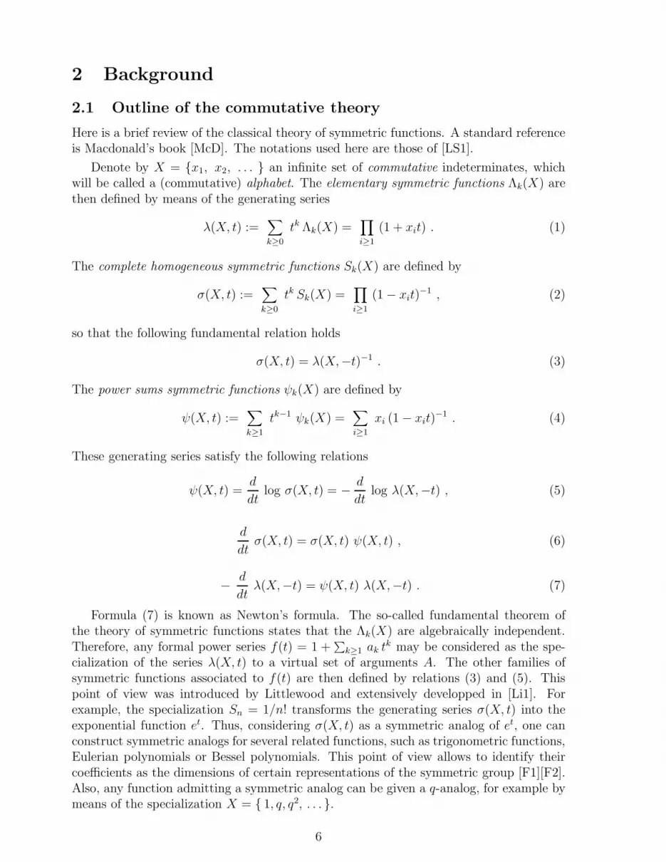
One can identify the tensor product Sym⊗ Sym with the algebra Sym(X, Y ) of poly-nomials which are separately symmetric in two infinite disjoint sets of indeterminates X

7

and Y , the correspondence being given by F ⊗G 7−→ F (X)G(Y ). Denoting by X+Y thedisjoint union of X and Y , one can then define a comultiplication ∆ on Sym by setting∆(F ) = F (X + Y ). This comultiplication endows Sym with the structure of a self-dual Hopf algebra, which is very useful for calculations involving characters of symmetricgroups (see for instance [Gei], [Zel], [ST] or [Th]). The basic formulas are

(F1F2 · · ·Fr) ∗G = µr[(F1 ⊗ F2 ⊗ · · · ⊗ Fr) ∗∆rG] , (10)

where µr denotes the r-fold ordinary multiplication and ∆r the iterated coproduct, and

∆r(F ∗G) = ∆r(F ) ∗∆r(G) . (11)

It will be shown in the sequel that both of these formulas admit natural noncommutativeanalogs. The antipode of the Hopf algebra Sym is given, in λ-ring notation, by

ω(F (X)) = F (−X) . (12)

The symmetric functions of (−X) are defined by the generating series

λ(−X, t) := σ(X,−t) = [λ(X, t)]−1 (13)

and one can more generally consider differences of alphabets. The symmetric functionsof X − Y are given by the generating series

λ(X − Y, t) := λ(X, t) λ(−Y, t) = λ(X, t) σ(Y,−t) . (14)

In particular, ψk(X − Y ) = ψk(X)− ψk(Y ).

There is another coproduct δ on Sym, which is obtained by considering productsinstead of sums, that is

δ(F ) = F (XY ) . (15)

One can check that its adjoint is the internal product :

(δF , P ⊗Q) = (F , P ∗Q) . (16)

This equation can be used to give an intrinsic definition of the internal product, i.e.without any reference to characters of the symmetric group. Also, one can see that twobases (UI), (VJ) of Sym are adjoint to each other iff

σ(XY, 1) =∑

I

UI(X)VI(Y ) . (17)

For example, writing σ(XY, 1) =∏

i σ(Y, xi) and expanding the product, one obtainsthat the adjoint basis of SI is formed by the monomial functions ψI .

2.2 Quasi-determinants

Quasi-determinants have been defined in [GR1] and further developed in [GR2] and [KL].In this section we briefly survey their main properties, the reader being referred to thesepapers for a more detailed account.

8

Let K be a field, n an integer and A = aij, 1 ≤ i, j ≤ n an alphabet of order n2,i.e. a set of n2 noncommutative indeterminates. Let K 6<A 6> be the free field constructedon K and generated by A. This is the universal field of fractions of the free associativealgebra K〈A〉 (cf. [Co]). The matrix A = (aij)1≤i,j≤n is called the generic matrix of ordern. This matrix is invertible over K 6<A 6>.

Let Apq denote the matrix obtained from the generic matrix A by deleting the p-th rowand the q-th column. Let also ξpq = (ap1, . . . , apq, . . . , apn) and ηpq = (a1q, . . . , apq, . . . , anq).

Definition 2.1 The quasi-determinant |A|pq of order pq of the generic matrix A is theelement of K 6<A 6> defined by

|A|pq = apq − ξpq (Apq)−1 ηpq = apq −∑

i6=p,j 6=q

apj ((Apq)−1)ji aiq .

It is sometimes convenient to adopt the following more explicit notation

|A|pq =

∣∣∣∣∣∣∣∣∣∣∣∣∣

a11 . . . a1q . . . a1n...

......

ap1 . . . apq . . . apn

......

...an1 . . . anq . . . ann

∣∣∣∣∣∣∣∣∣∣∣∣∣

.

Quasi-determinants are here only defined for generic matrices. However, using substitu-tions, this definition can be applied to matrices with entries in an arbitrary skew field.In fact, one can even work in a noncommutative ring, provided that Apq be an invertiblematrix.

Example 2.2 For n = 2, there are four quasi-determinants :∣∣∣∣a11 a12

a21 a22

∣∣∣∣ = a11 − a12 a−122 a21 ,

∣∣∣∣a11 a12

a21 a22

∣∣∣∣ = a12 − a11 a−121 a22 ,

∣∣∣∣a11 a12

a21 a22

∣∣∣∣ = a21 − a22 a−112 a11 ,

∣∣∣∣a11 a12

a21 a22

∣∣∣∣ = a22 − a21 a−111 a12 .

The next result can be considered as another definition of quasi-determinants (forgeneric matrices).

Proposition 2.3 Let A be the generic matrix of order n and let B = A−1 = (bpq)1≤p,q≤n

be its inverse. Then one has |A|pq = b−1qp for every 1 ≤ p, q ≤ n.

It follows from Proposition 2.3 that |A|pq = (−1)p+q detA/detApq when the aij arecommutative variables. Thus quasi-determinants are noncommutative analogs of the ratioof a determinant to one of its principal minors. If A is an invertible matrix with entriesin a arbitrary skew field, the above relation still holds for every p, q such that bqp 6= 0.Another consequence of Proposition 2.3 is that

|A|pq = apq −∑

i6=p,j 6=q

apj |Apq|−1

ij aiq ,

which provides a recursive definition of quasi-determinants.

9

Let I be the unit matrix of order n. The expansions of the quasi-determinants of I−Ainto formal power series are conveniently described in terms of paths in a graph. Let An

denote the complete oriented graph with n vertices 1, 2, . . . , n , the arrow from i to jbeing labelled by aij . We denote by Pij the set of words labelling a path in An going fromi to j, i.e. the set of words of the form w = aik1 ak1k2 ak2k3 . . . akr−1j . A simple path is apath such that ks 6= i, j for every s. We denote by SP ij the set of words labelling simplepaths from i to j.

Proposition 2.4 Let i, j be two distinct integers between 1 and n. Then,

|I −A|ii = 1−∑

SPii

w , |I −A|−1ij =

∑

Pji

w . (18)

Example 2.5 For n = 2,

∣∣∣∣1− a11 −a12

−a21 1− a22

∣∣∣∣ = 1− a11 −∑

p≥0

a12 ap22 a21 .

As a general rule, quasi-determinants are not polynomials in their entries, except inthe following special case, which is particularly important for noncommutative symmetricfunctions (a graphical interpretation of this formula can be found in the Appendix).

Proposition 2.6 The following quasi-determinant is a polynomial in its entries :

∣∣∣∣∣∣∣∣∣∣∣∣

a11 a12 a13 . . . a1n

−1 a22 a23 . . . a2n

0 −1 a33. . .

......

. . .. . .

. . . an−1 n

0 . . . 0 −1 ann

∣∣∣∣∣∣∣∣∣∣∣∣

= a1n+∑

1≤j1<j2<...<jk<n

a1j1 aj1+1 j2 aj2+1 j3 . . . ajk+1 n . (19)

We now recall some useful properties of quasi-determinants. Quasi-determinants be-have well with respect to permutation of rows and columns.

Proposition 2.7 A permutation of the rows or columns of a quasi-determinant does notchange its value.

Example 2.8

∣∣∣∣∣∣∣

a11 a12 a13

a21 a22 a23

a31 a32 a33

∣∣∣∣∣∣∣=

∣∣∣∣∣∣∣

a21 a22 a23

a11 a12 a13

a31 a32 a33

∣∣∣∣∣∣∣=

∣∣∣∣∣∣∣

a22 a21 a23

a12 a11 a13

a32 a31 a33

∣∣∣∣∣∣∣.

One can also give the following analogs of the classical behaviour of a determinant withrespect to linear combinations of rows and columns.

10

Proposition 2.9 If the matrix B is obtained from the matrix A by multiplying the p-throw on the left by λ, then

|B|kq =λ |A|pq for k = p ,|A|kq for k 6= p .

Similarly, if the matrix C is obtained from the matrix A by multiplying the q-th columnon the right by µ, then

|C|pl =|A|pq µ for l = q ,|A|pl for l 6= q .

Finally, if the matrix D is obtained from A by adding to some row (resp. column) of Aits k-th row (resp. column), then |D|pq = |A|pq for every p 6= k (resp. q 6= k).

The following proposition gives important identities which are called homological re-lations.

Proposition 2.10 The quasi-minors of the generic matrix A are related by :

|A|ij (|Ail|kj)−1 = −|A|il (|Aij |kl)

−1 ,

(|Akj|il)−1 |A|ij = −(|Aij |kl)−1 |A|kj .

Example 2.11

∣∣∣∣a11 a12

a31 a32

∣∣∣∣−1

∣∣∣∣∣∣∣

a11 a12 a13

a21 a22 a23

a31 a32 a33

∣∣∣∣∣∣∣= −

∣∣∣∣a11 a12

a21 a22

∣∣∣∣−1

∣∣∣∣∣∣∣

a11 a12 a13

a21 a22 a23

a31 a32 a33

∣∣∣∣∣∣∣.

The classical expansion of a determinant by one of its rows or columns is replaced bythe following property.

Proposition 2.12 For quasi-determinants, there holds :

|A|pq = apq −∑

j 6=q

apj (|Apq|kj)−1 |Apj|kq ,

|A|pq = apq −∑

i6=p

|Aiq|pl (|Apq|il)

−1 aiq ,

for every k 6= p and l 6= q.

Example 2.13 Let n = p = q = 4. Then,

∣∣∣∣∣∣∣∣∣

a11 a12 a13 a14

a21 a22 a23 a24

a31 a32 a33 a34

a41 a42 a43 a44

∣∣∣∣∣∣∣∣∣= a44 − a43

∣∣∣∣∣∣∣

a11 a12 a13

a21 a22 a23

a31 a32 a33

∣∣∣∣∣∣∣

−1 ∣∣∣∣∣∣∣

a11 a12 a14

a21 a22 a24

a31 a32 a34

∣∣∣∣∣∣∣

− a42

∣∣∣∣∣∣∣

a11 a12 a13

a21 a22 a23

a31 a32 a33

∣∣∣∣∣∣∣

−1 ∣∣∣∣∣∣∣

a11 a13 a14

a21 a23 a24

a31 a33 a34

∣∣∣∣∣∣∣− a41

∣∣∣∣∣∣∣

a11 a12 a13

a21 a22 a23

a31 a32 a33

∣∣∣∣∣∣∣

−1 ∣∣∣∣∣∣∣

a12 a13 a14

a22 a23 a24

a32 a33 a34

∣∣∣∣∣∣∣.

11

Let P, Q be subsets of 1, . . . , n of the same cardinality. We denote by APQ thematrix obtained by removing from A the rows whose indices belong to P and the columnswhose indices belong to Q. Also, we denote by APQ the submatrix of A whose row indicesbelong to P and column indices to Q. Finally, if aij is an entry of some submatrix APQ

or APQ, we denote by |APQ|ij or |APQ|ij the corresponding quasi-minor.

Here is a noncommutative version of Jacobi’s ratio theorem which relates the quasi-minors of a matrix with those of its inverse. This identity will be frequently used in thesequel.

Theorem 2.14 Let A be the generic matrix of order n, let B be its inverse and let(i, L, P ) and (j,M,Q) be two partitions of 1, 2, . . . , n such that |L| = |M | and|P | = |Q|. Then, one has

|BM∪j,L∪i|ji = |AP∪i,Q∪j|−1ij .

Example 2.15 Take n = 5, i = 3, j = 4, L = 1, 2, M = 1, 3, P = 4, 5 andQ = 2, 5. There holds

∣∣∣∣∣∣∣

a32 a34 a35

a42 a44 a45

a52 a54 a55

∣∣∣∣∣∣∣=

∣∣∣∣∣∣∣

b11 b12 b13b31 b32 b33b41 b42 b43

∣∣∣∣∣∣∣

−1

.

We conclude with noncommutative versions of Sylvester’s and Bazin’s theorems.

Theorem 2.16 Let A be the generic matrix of order n and let P,Q be two subsets of[1, n] of cardinality k. For i /∈ P and j /∈ Q, we set bij = |AP∪i,Q∪j|ij and form thematrix B = (bij)i/∈P,j /∈Q of order n− k. Then,

|A|lm = |B|lm

for every l /∈ P and every m /∈ Q.

Example 2.17 Let us take n = 3, P = Q = 3 and l = m = 1. Then,

∣∣∣∣∣∣∣

a11 a12 a13

a21 a22 a23

a31 a32 a33

∣∣∣∣∣∣∣=

∣∣∣∣∣∣∣∣∣

∣∣∣∣a11 a13

a31 a33

∣∣∣∣∣∣∣∣a12 a13

a32 a33

∣∣∣∣∣∣∣∣a22 a23

a32 a33

∣∣∣∣∣∣∣∣a21 a23

a31 a33

∣∣∣∣

∣∣∣∣∣∣∣∣∣.

Let A be a matrix of order n×p, where p ≥ n. Then, for every subset P of cardinalityn of 1, . . . , p, we denote by AP the square submatrix of A whose columns are indexedby P .

Theorem 2.18 Let A be the generic matrix of order n×2n and let m be an integer in1, . . . , n. For 1 ≤ i, j ≤ n, we set bij = |Aj,n+1,...,n+i−1,n+i+1,...,2n|mj and form thematrix B = (bij)1≤i,j≤n. Then we have

|B|kl = |An+1,...,2n|m,n+k |A1,...,l−1,l+1,...,n,n+k|−1m,n+k |A1,...,n|ml

for every integers k, l in 1, . . . , n.

12

Example 2.19 Let n = 3 and k = l = m = 1. Let us adopt more appropriate notations,writing for example |245| instead of |M2,4,5|14. Bazin’s identity reads

∣∣∣∣∣∣∣

|156| |256| |356||146| |246| |346||145| |245| |345|

∣∣∣∣∣∣∣= |456| |234 |−1 |123| .

We shall also need the following variant of Bazin’s theorem 2.18.

Theorem 2.20 Let A be the generic matrix of order n×(3n− 2) and let m be an integerin 1, . . . , n. For 1 ≤ i, j ≤ n, we set cij = |Aj,n+i,n+i+1,...,2n+i−2|mj and form the matrixC = (cij)1≤i,j≤n. Then we have

|C|11 = |An+1,...,2n|m,2n |A2,3...,n,2n|−1m,2n |A1,...,n|m1 .

Example 2.21 Let n = 3, m = 1, and keep the notations of 2.19. Theorem 2.20 reads

∣∣∣∣∣∣∣

|145| |245| |345||156| |256| |356||167| |267| |367|

∣∣∣∣∣∣∣= |456 | |236 |−1 |123| . (20)

Proof — We use an induction on n. For n = 2, Theorem 2.20 reduces to Theorem 2.18.For n = 3, we have to prove (20). To this end, we note that the specialization 7→ 4 givesback Bazin’s theorem 2.18. Since the right-hand side does not contain 7, it is thereforeenough to show that the left-hand side does not depend on 7. But by Sylvester’s theorem2.16, the left-hand side is equal to

∣∣∣∣|145| |245||156| |256|

∣∣∣∣−∣∣∣∣|245| |345||256| |356|

∣∣∣∣∣∣∣∣|256| |356||267| |367|

∣∣∣∣−1 ∣∣∣∣|156| |256|| 167| |267|

∣∣∣∣

= |456 | |256 |−1 |125| − |456 | |256 |−1 |235||236|−1|126| ,

which is independent of 7. Here, the second expression is derived by means of 2.18 andMuir’s law of extensible minors for quasi-determinants [KL]. The general induction stepis similar, and we shall not detail it. 2

13

3 Formal noncommutative symmetric functions

In this section, we introduce the algebra Sym of formal noncommutative symmetricfunctions which is just the free associative algebra K〈Λ1,Λ2, . . .〉 generated by an infinitesequence of indeterminates (Λk)k≥1 over some fixed commutative field K of characteristiczero. This algebra will be graded by the weight function w(Λk) = k. The homogeneouscomponent of weight n will be denoted by Symn. The Λk will be informally regardedas the elementary symmetric functions of some virtual set of arguments. When we needseveral copies of Sym, we can give them labels A,B, . . . and use the different sets ofindeterminates Λk(A),Λk(B), . . . together with their generating series λ(A, t), λ(B, t), . . .,and so on. The corresponding algebras will be denoted Sym(A), Sym(B), etc.

We recall that a composition is a vector I = (i1, . . . , ik) of nonnegative integers, calledthe parts of I. The length l(I) of the composition I is the number k of its parts and theweigth of I is the sum |I| =

∑ij of its parts.

3.1 Elementary, complete and power sums functions

Let t be another indeterminate, commuting with all the Λk. It will be convenient in thesequel to set Λ0 = 1.

Definition 3.1 The elementary symmetric functions are the Λk themselves, and theirgenerating series is denoted by

λ(t) :=∑

k≥0

tk Λk = 1 +∑

k≥1

tk Λk . (21)

The complete homogeneous symmetric functions Sk are defined by

σ(t) :=∑

k≥0

tk Sk = λ(−t)−1 . (22)

The power sums symmetric functions of the first kind Ψk are defined by

ψ(t) :=∑

k≥1

tk−1 Ψk , (23)

d

dtσ(t) = σ(t) ψ(t) . (24)

The power sums symmetric functions of the second kind Φk are defined by

σ(t) = exp (∑

k≥1

tkΦk

k) , (25)

or equivalently by one of the series

Φ(t) :=∑

k≥1

tkΦk

k= log ( 1 +

∑

k≥1

Sk tk ) (26)

or

φ(t) :=∑

k≥1

tk−1 Φk =d

dtΦ(t) =

d

dtlog σ(t) . (27)

14

Although the two kinds of power sums coincide in the commutative case, they arequite different at the noncommutative level. For instance,

Φ3 = Ψ3 +1

4(Ψ1 Ψ2 −Ψ2 Ψ1) . (28)

The appearance of two families of power sums is due to the fact that one does not have aunique notion of logarithmic derivative for power series with noncommutative coefficients.The two families selected here correspond to the most natural noncommutative analogs.We shall see below that both of them admit interesting interpretations in terms of Liealgebras. Moreover, they may be related to each other via appropriate specializations (cf.Note 5.14).

One might also introduce a third family of power sums by replacing (24) by

d

dtσ(t) = ψ(t) σ(t) ,

but this would lead to essentially the same functions. Indeed, Sym is equiped with severalnatural involutions, among which the anti-automorphism which leaves invariant the Λk.Denote this involution by F −→ F ∗. It follows from (22) and (26) that one also hasS∗

k = Sk, Φ∗k = Φk, and,

d

dtσ(t) = ψ(t)∗ σ(t) ,

with ψ(t)∗ =∑

k≥1 tk−1 Ψ∗k.

Other involutions, to be defined below, send Λk on ±Sk. This is another way to handlethe left-right symmetry in Sym, as shown by the following proposition which expressesψ(t) in terms of λ(t).

Proposition 3.2 One has

−d

dtλ(−t) = ψ(t) λ(−t) . (29)

Proof — Multiplying from left and right equation (24) by λ(−t), we obtain

λ(−t)

(d

dtσ(t)

)λ(−t) = σ(t)−1

(d

dtσ(t)

)σ(t)−1 = ψ(t) λ(−t) .

But one also has

σ(t)−1

(d

dtσ(t)

)σ(t)−1 = −

d

dtσ(t)−1 = −

d

dtλ(−t) .

2

These identities between formal power series imply the following relations betweentheir coefficients.

15

Proposition 3.3 For n ≥ 1, one has

n∑

k=0

(−1)n−k Sk Λn−k =n∑

k=0

(−1)n−k Λk Sn−k = 0 , (30)

n−1∑

k=0

Sk Ψn−k = nSn ,n−1∑

k=0

(−1)n−k−1 Ψn−k Λk = nΛn . (31)

Proof — Relation (30) is obtained by considering the coefficient of tn in the definingequalities σ(t)λ(−t) = λ(−t) σ(t) = 1. The other identity is proved similarly from rela-tions (24) and (29). 2

In the commutative case, formulas (30) and (31) are respectively called Wronski andNewton formulas.

It follows from relation (26) that for n ≥ 1

Φn = nSn +∑

i1+...+im=n,m>1

ci1,...,im Si1 . . . Sim (32)

where ci1,...,im are some rational constants, so that Proposition 3.3 implies in particularthat Sym is freely generated by any of the families (Sk), (Ψk) or (Φk). This observationleads to the following definitions.

Definition 3.4 Let I = (i1, . . . , in) ∈ (N∗)n be a composition. One defines the productsof complete symmetric functions

SI = Si1 Si2 . . . Sin . (33)

Similarly, one has the products of elementary symmetric functions

ΛI = Λi1 Λi2 . . . Λin , (34)

the products of power sums of the first kind

ΨI = Ψi1 Ψi2 . . . Ψin , (35)

and the products of power sums of the second kind

ΦI = Φi1 Φi2 . . . Φin . (36)

Note 3.5 As in the classical case, the complete and elementary symmetric functions formZ-bases of Sym (i.e. bases of the algebra generated over Z by the Λk) while the powersums of first and second kind are just Q-bases.

The systems of linear equations given by Proposition 3.3 can be solved by means ofquasi-determinants. This leads to the following quasi-determinantal formulas.

16

Corollary 3.6 For every n ≥ 1, one has

Sn = (−1)n−1

∣∣∣∣∣∣∣∣∣∣∣∣

Λ1 Λ2 . . . Λn−1 Λn

Λ0 Λ1 . . . Λn−2 Λn−1

0 Λ0 . . . Λn−3 Λn−2...

.... . .

......

0 0 . . . Λ0 Λ1

∣∣∣∣∣∣∣∣∣∣∣∣

, (37)

Λn = (−1)n−1

∣∣∣∣∣∣∣∣∣∣∣∣

S1 S0 0 . . . 0S2 S1 S0 . . . 0S3 S2 S1 . . . 0...

......

. . ....

Sn Sn−1 Sn−2 . . . S1

∣∣∣∣∣∣∣∣∣∣∣∣

, (38)

nSn =

∣∣∣∣∣∣∣∣∣∣∣∣

Ψ1 Ψ2 . . . Ψn−1 Ψn

−1 Ψ1 . . . Ψn−2 Ψn−1

0 −2 . . . Ψn−3 Ψn−2...

.... . .

......

0 0 . . . −n + 1 Ψ1

∣∣∣∣∣∣∣∣∣∣∣∣

, (39)

nΛn =

∣∣∣∣∣∣∣∣∣∣∣∣

Ψ1 1 0 . . . 0Ψ2 Ψ1 2 . . . 0Ψ3 Ψ2 Ψ1 . . . 0...

......

. . ....

Ψn Ψn−1 Ψn−2 . . . Ψ1

∣∣∣∣∣∣∣∣∣∣∣∣

, (40)

Ψn =

∣∣∣∣∣∣∣∣∣∣∣∣

S1 S0 0 . . . 02S2 S1 S0 . . . 03S3 S2 S1 . . . 0...

......

. . ....

nSn Sn−1 Sn−2 . . . S1

∣∣∣∣∣∣∣∣∣∣∣∣

=

∣∣∣∣∣∣∣∣∣∣∣∣

Λ1 2Λ2 . . . (n− 1)Λn−1 nΛn

Λ0 Λ1 . . . Λn−2 Λn−1

0 Λ0 . . . Λn−3 Λn−2...

.... . .

......

0 0 . . . Λ0 Λ1

∣∣∣∣∣∣∣∣∣∣∣∣

. (41)

Proof — Formulas (37) and (38) follow from relations (30) by means of Theorem 1.8 of[GR1]. The other formulas are proved in the same way. 2

Note 3.7 In the commutative theory, many determinantal formulas can be obtained fromNewton’s relations. Most of them can be lifted to the noncommutative case, as illustratedon the following relations, due to Mangeot in the commutative case (see [LS1]).

(−1)n−1 nSn =

∣∣∣∣∣∣∣∣∣∣∣∣

2 Λ1 1 0 . . . 04 Λ2 3 Λ1 2 Λ0 . . . 0

......

......

(2n− 2) Λn−1 (2n− 3) Λn−2 (2n− 4) Λn−3 . . . (n− 1) Λ0

nΛn (n− 1) Λn−1 (n− 2) Λn−2 . . . Λ1

∣∣∣∣∣∣∣∣∣∣∣∣

. (42)

17

To prove this formula, it suffices to note that, using relations (31), one can show as in thecommutative case that the matrix involved in (42) is the product of the matrix

Ψ =

Ψ1 1 0 . . . 0−Ψ2 Ψ1 2 . . . 0Ψ3 −Ψ2 Ψ1 . . . 0...

......

...(−1)n−1 Ψn (−1)n−2 Ψn−1 (−1)n−3 Ψn−2 . . . Ψ1

by the matrix Λ = (Λj−i)0≤i,j≤n−1. Formula (42) then follows from Theorem 1.7 of [GR1].

Proposition 3.3 can also be interpreted in the Hopf algebra formalism. Let us considerthe comultiplication ∆ defined in Sym by

∆(Ψk) = 1⊗Ψk + Ψk ⊗ 1 (43)

for k ≥ 1. Then, as in the commutative case (cf. [Gei] for instance), the elementary andcomplete functions form infinite sequences of divided powers.

Proposition 3.8 For every k ≥ 1, one has

∆(Sk) =k∑

i=0

Si ⊗ Sk−i , ∆(Λk) =k∑

i=0

Λi ⊗ Λk−i .

Proof — We prove the claim for ∆(Sk), the other proof being similar. Note first thatthere is nothing to prove for k = 0 and k = 1. Using now induction on k and relation(31), we obtain

k∆(Sk) =k−1∑

i=0

i∑

j=0

(Sj ⊗ Si−jΨk−i + Si−jΨk−i ⊗ Sj)

=k−1∑

j=0

Sj ⊗ (k−1∑

i=j

Si−jΨk−i) +k−1∑

j=0

(k−1∑

i=j

Si−jΨk−i)⊗ Sj

=k−1∑

j=0

(Sj ⊗ (k − j)Sk−j) +k−1∑

j=0

(k − j)Sk−j ⊗ Sj = kk∑

j=0

(Sj ⊗ Sk−j) .

2

We define an anti-automorphism ω of Sym by setting

ω(Sk) = Λk (44)

for k ≥ 0. The different formulas of Corollary 3.6 show that

ω(Λk) = Sk , ω(Ψk) = (−1)k−1 Ψk .

In particular we see that ω is an involution. To summarize:

18

Proposition 3.9 The comultiplication ∆ and the antipode ω, where ω is the anti-auto-morphism of Sym defined by

ω(Sk) = (−1)k Λk, k ≥ 0 , (45)

endow Sym with the structure of a Hopf algebra.

The following property, which is equivalent to the Continuous Baker-Campbell-Hausdorfftheorem of Magnus [Mag] and Chen [C2], has some interesting consequences.

Proposition 3.10 The Lie algebra generated by the family (Φk) coincides with the Liealgebra generated by the family (Ψk). We shall denote it by L(Ψ). Moreover the differenceΦk −Ψk lies in the Lie ideal L2(Ψ) for every k ≥ 1.

Proof — In order to see that the two Lie algebras L(Ψ) and L(Φ) coincide, it is sufficientto show that Φ lies in L(Ψ). According to Friedrichs’ criterion (cf. [Re] for instance),we just have to check that Φ is primitive for the comultiplication ∆. Using (26) andProposition 3.8, we can now write

∑

k≥1

tk∆(Φk)

k= log (

∑

k≥0

∆(Sk) tk ) = log (UV ) , (46)

where we respectively set U =∑

k≥0 (1 ⊗ Sk) tk and V =

∑k≥0 (Sk ⊗ 1) tk. Since all

coefficients of U commute with all coefficients of V , we have log(UV ) = log(U) + log(V )from which, applying again (26), we obtain

∑

k≥1

tk∆(Φk)

k=∑

k≥1

tk1⊗ Φk

k+

∑

k≥1

tkΦk ⊗ 1

k, (47)

as required. The second point follows from the fact that Φk −Ψk is of order at least 2 inthe Ψi, which is itself a consequence of (32). 2

Example 3.11 The first Lie relations between Φk and Ψk are given below.

Φ1 = Ψ1, Φ2 = Ψ2, Φ3 = Ψ3 +1

4[Ψ1,Ψ2], Φ4 = Ψ4 +

1

3[Ψ1,Ψ3],

Φ5 = Ψ5 +3

8[Ψ1,Ψ4] +

1

12[Ψ2,Ψ3] +

1

72[Ψ1, [Ψ1,Ψ3]]

+1

48[[Ψ1,Ψ2],Ψ2] +

1

144[[[Ψ2,Ψ1],Ψ1],Ψ1] .

It is worth noting that, according to Proposition 3.10, the Hopf structures defined byrequiring the Φk or the Ψk to be primitive are the same. Note also that the antipodalproperty of ω and the fact that

∆(Φk) = 1⊗ Φk + Φk ⊗ 1 (48)

show that we haveω(Φk) = (−1)k−1 Φk . (49)

19

3.2 Ribbon Schur functions

A general notion of quasi-Schur function can be obtained by replacing the classical Jacobi-Trudi determinant by an appropriate quasi-determinant (see Section 3.3). However, asmentioned in the introduction, these expressions are no longer polynomials in the gene-rators of Sym, except in one case. This is when all the subdiagonal elements ai+1,i of theirdefining quasi-determinant are scalars, which corresponds to Schur functions indexed byribbon shaped diagrams. We recall that a ribbon or skew-hook is a skew Young diagramcontaining no 2 × 2 block of boxes. For instance, the skew diagram Θ = I/J withI = (3, 3, 3, 6, 7) and J = (2, 2, 2, 5)

is a ribbon. A ribbon Θ with n boxes is naturally encoded by a composition I = (i1, . . . , ir)of n, whose parts are the lengths of its rows (starting from the top). In the above example,we have I = (3, 1, 1, 4, 2). Following [MM], we also define the conjugate composition I∼

of I as the one whose associated ribbon is the conjugate (in the sense of skew diagrams)of the ribbon of I. For example, with I = (3, 1, 1, 4, 2), we have I∼ = (1, 2, 1, 1, 4, 1, 1).

In the commutative case, the skew Schur functions indexed by ribbon diagrams possessinteresting properties and are strongly related to the combinatorics of compositions anddescents of permutations (cf. [Ge], [GeR] or [Re] for instance). They have been definedand investigated by MacMahon (cf. [MM]). Although the commutative ribbon functionsare not linearly independent, e.g. R12 = R21, it will be shown in Section 4 that thenoncommutative ones form a linear basis of Sym.

Definition 3.12 Let I = (i1, . . . , in) ∈ (N∗)n be a composition. Then the ribbon Schurfunction RI is defined by

RI = (−1)n−1

∣∣∣∣∣∣∣∣∣∣∣∣

Si1 Si1+i2 Si1+i2+i3 . . . Si1+...+in

S0 Si2 Si2+i3 . . . Si2+...+in

0 S0 Si3 . . . Si3+...+in...

......

. . ....

0 0 0 . . . Sin

∣∣∣∣∣∣∣∣∣∣∣∣

(50)

As in the commutative case, we have Sn = Rn and Λn = R1n according to Corollary 3.6.Moreover, the ribbon functions R(1k ,n−k) play a particular role. In the commutative case,they are the hook Schur functions, denoted S(1k ,n−k). We shall also use this notation forthe noncommutative ones.

We have for the multiplication of ribbon Schur functions the following formula, whosecommutative version is due to MacMahon (cf. [MM]).

Proposition 3.13 Let I = (i1, . . . , ir) and J = (j1, . . . , js) be two compositions. Then,

RI RJ = RI⊲J +RI·J

where I ⊲J denotes the composition (i1, . . . , ir−1, ir+j1, j2, . . . , js) and I ·J the composition(i1, . . . , ir, j1, . . . , js).

20

Proof — Using the above notations, we can write that RI is equal to

(−1)k−1

∣∣∣∣∣∣∣∣∣∣

Si1 . . . Si1+...+ik−1

S0 . . . Si2+...+ik−1

......

0 . . . Sik−1

∣∣∣∣∣∣∣∣∣∣

∣∣∣∣∣∣∣∣∣∣

S0 . . . Si2+...+ik−1

0 . . . Si3+...+ik−1

......

0 . . . S0

∣∣∣∣∣∣∣∣∣∣

−1 ∣∣∣∣∣∣∣∣∣∣

Si1 Si1+i2 . . . Si1+...+ik

S0 Si2 . . . Si2+...+ik...

.... . .

...0 0 . . . Sik

∣∣∣∣∣∣∣∣∣∣

,

= R(i1,...,ik−1) (Sik − R−1(i1,...,ik−1)

R(i1,...,ik−2,ik−1+ik)) ,

the first equality following from the homological relations between quasi-determinants ofthe same matrix, and the second one from the expansion of the last quasi-determinantby its last row together with the fact that the second quasi-determinant involved in thisrelation is equal to 1. Hence,

RI Rn = RI⊲n +RI·n . (51)

Thus, the proposition holds for ℓ(J) = 1. Let now J = (j1, . . . , jn) and J ′ = (j1, . . . , jn−1).Then relation (51) shows that

RJ = RJ ′ Rjn− RJ ′⊲jn

.

Using this last identity together with induction on ℓ(J), we get

RI RJ = RI⊲J ′ Rjn+RI·J ′ Rjn

−RI⊲(J ′⊲jn) − RI·(J ′⊲jn) ,

and the conclusion follows by means of relation (51) applied two times. 2

Proposition 3.13 shows in particular that the product of an elementary by a completefunction is the sum of two hook functions,

Λk Sl = R1kl +R1k−1(l+1) . (52)

We also note the following expression of the power sums Ψn in terms of hook Schurfunctions.

Corollary 3.14 For every n ≥ 1, one has

Ψn =n−1∑

k=0

(−1)k R1k(n−k) .

Proof — The identity λ(−t)d

dtσ(t) = ψ(t) implies that

Ψn =n−1∑

k=0

(−1)k (n− k) Λk Sn−k , (53)

and the result follows from (52). 2

Let us introduce the two infinite Toeplitz matrices

S = (Sj−i)i,j≥0 , Λ =((−1)j−i Λj−i

)i,j≥0

, (54)

21

where we set Sk = Λk = 0 for k < 0. The identity λ(−t) σ(t) = σ(t) λ(−t) = 1 isequivalent to the fact that Λ S = S Λ = I. We know that the quasi-minors of theinverse matrix A−1 are connected with those of A by Jacobi’s ratio theorem for quasi-determinants (Theorem 2.14). Thus the ribbon functions may also be expressed in termsof the Λk, as shown by the next proposition.

Proposition 3.15 Let I ∈ Nn be a composition and let I∼ = (j1, . . . , jm) be the conjugatecomposition. Then one has the relation

RI = (−1)m−1

∣∣∣∣∣∣∣∣∣∣∣∣

ΛjmΛjm−1+jm

Λjm−2+jm−1+jm. . . Λj1+...+jm

Λ0 Λjm−1 Λjm−2+jm−1 . . . Λj1+...+jm−1

0 Λ0 Λjm−2 . . . Λj1+...+jm−2

......

.... . .

...0 0 0 . . . Λj1

∣∣∣∣∣∣∣∣∣∣∣∣

.

Proof — This formula is obtained by applying Jacobi’s theorem for quasi-determinants(Theorem 2.14) to the definition of RI . 2

Corollary 3.16 For any composition I, one has

ω(RI) = RI∼.

3.3 Quasi-Schur functions

We shall now consider general quasi-minors of the matrices S and Λ and proceed to thedefinition of quasi-Schur functions. As already mentioned, they are no longer elements ofSym, but of the free field K 6<S1, S2, . . . 6> generated by the Si.

Definition 3.17 Let I = (i1, i2, . . . , in) be a partition, i.e. a weakly increasing sequenceof nonnegative integers. We define the quasi-Schur function SI by setting

SI = (−1)n−1

∣∣∣∣∣∣∣∣∣∣

Si1 Si2+1 . . . Sin+n−1

Si1−1 Si2 . . . Sin+n−2...

.... . .

...Si1−n+1 Si2−n+2 . . . Sin

∣∣∣∣∣∣∣∣∣∣

. (55)

In particular we have Si = Si, S1i = Λi and S1i(n−i) = R1i(n−i). However it must be

noted that for a general partition I, the quasi-Schur function SI reduces in the commuta-tive case to the ratio of two Schur functions SI/SJ , where J = (i1−1, i2−1, . . . , in−1−1).One can also define in the same way skew Schur functions. One has to take the sameminor as in the commutative case, with the box in the upper right corner and the sign(−1)n−1, where n is the order of the quasi-minor. The ribbon Schur functions are the onlyquasi-Schur functions which are polynomials in the Sk, and they reduce to the ordinaryribbon functions in the commutative case. To emphasize this point, we shall also denotethe quasi-Schur function SI/J by SI/J when I/J is a ribbon.

Quasi-Schur functions are indexed by partitions. It would have been possible to definemore general functions indexed by compositions, but the homological relations imply

22

that such functions can always be expressed as noncommutative rational fractions in thequasi-Schur functions. For instance

S42 = −∣∣∣∣S4 S3

S3 S2

∣∣∣∣ = −∣∣∣∣S3 S4

S2 S3

∣∣∣∣ =∣∣∣∣S3 S4

S2 S3

∣∣∣∣ S−13 S2 = S33 S

−13 S2 .

Definition 3.17 is a noncommutative analog of the so-called Jacobi-Trudi formula.Using Jacobi’s theorem for the quasi-minors of the inverse matrix as in the proof ofProposition 3.15, we derive the following analog of Naegelbasch’s formula.

Proposition 3.18 Let I be a partition and let I∼ = (j1, . . . , jp) be its conjugate partition,i.e. the partition whose diagram is obtained by interchanging the rows and columns of thediagram of I. Then,

SI = (−1)p−1

∣∣∣∣∣∣∣∣∣∣

ΛjpΛjp+1 . . . Λjp+p−1

Λjp−1−1 Λjp−1 . . . Λjp−1+p−2

......

. . ....

Λj1−p+1 Λj1−p+2 . . . Λj1

∣∣∣∣∣∣∣∣∣∣

.

Let us extend ω to the skew field generated by the Sk. Then we have.

Proposition 3.19 Let I be a partition and let I∼ be its conjugate partition. There holds

ω(SI) = SI∼ .

Proof — This is a consequence of Proposition 3.18. 2

We can also extend the ∗ involution to the division ring generated by the Si. It followsfrom Definition 2.1 that S∗

I is equal to the transposed quasi-determinant

S∗I = (−1)n−1

∣∣∣∣∣∣∣∣∣∣

Sin Sin+1 . . . Sin+n−1

Sin−1−1 Sin−1 . . . Sin−1+n−2

......

. . ....

Si1−n+1 Si1−n+2 . . . Si1

∣∣∣∣∣∣∣∣∣∣

.

In particular, if I = nk is a rectangular partition, the quasi-Schur function indexed by Iis invariant under ∗.

In the commutative case, Schur functions can also be expressed as determinants ofhook Schur functions, according to a formula of Giambelli. This formula is stated moreconveniently, using Frobenius’ notation for partitions. In this notation, the hook

6

?

-

β

α

23

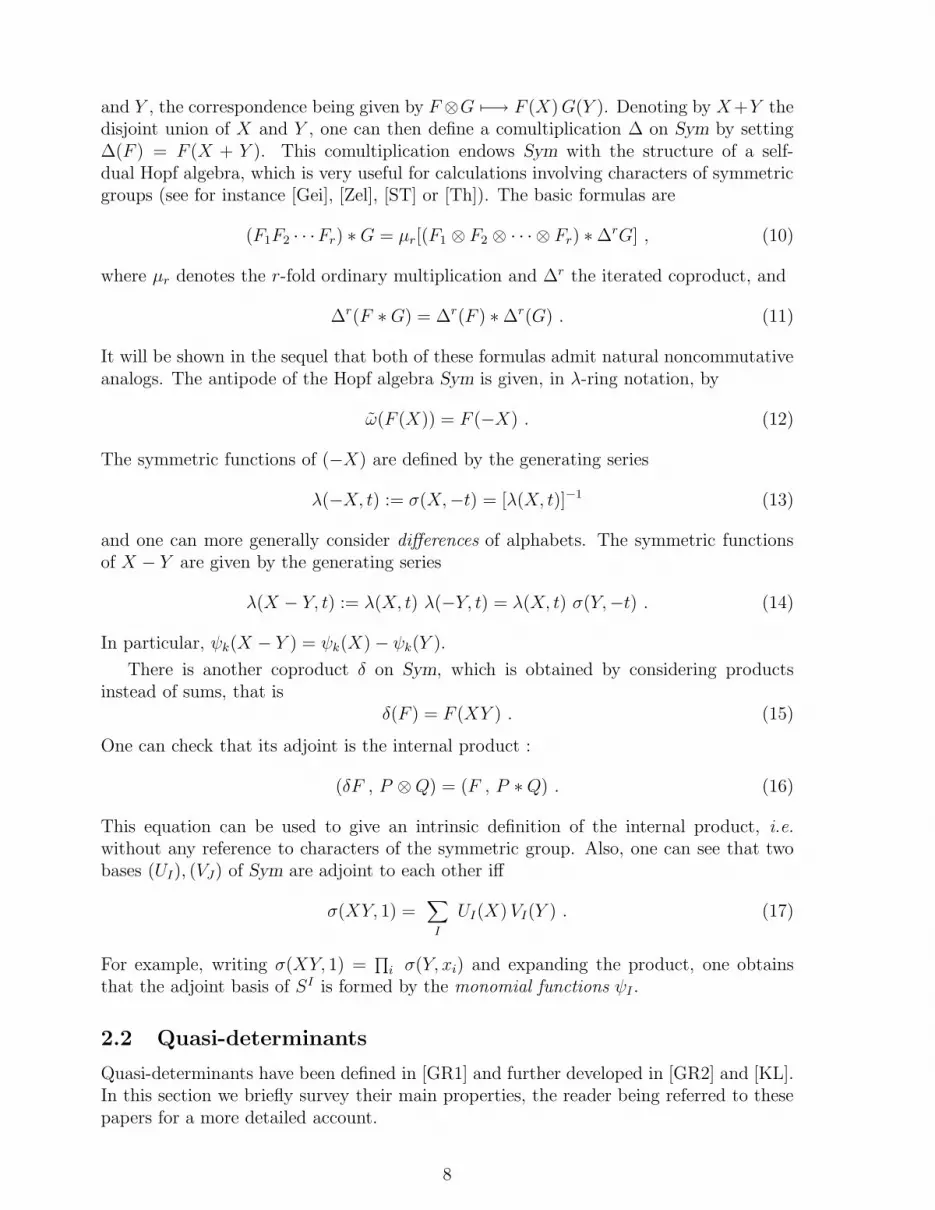
is written (β|α) := 1β (α + 1). A general partition is decomposed into diagonal hooks.Thus, for the partition I = (2, 3, 5, 7, 7) for instance, we have the following decomposition,where the different hooks are distinguished by means of the symbols ⋆, • and ⋄.

⋆ ⋆ ⋆ ⋆ ⋆ ⋆ ⋆⋆⋆⋆⋆

• • • • • ••••

⋄ ⋄ ⋄⋄

It is denoted (134 | 256) in Frobenius’ notation. We can now state.

Proposition 3.20 (Giambelli’s formula for quasi-Schur functions) Let I be a partitionrepresented by (β1 . . . βk | α1 . . . αk) in Frobenius’ notation. One has

SI =

∣∣∣∣∣∣∣∣∣∣

S(β1|α1) S(β1|α2) . . . S(β1|αk)

S(β2|α1) S(β2|α2) . . . S(β2|αk)

......

. . ....

S(βk |α1) S(βk|α2) . . . S(βk|αk)

∣∣∣∣∣∣∣∣∣∣

.

Proof — This is an example of relation between the quasi-minors of the matrix S. Theproposition is obtained by means of Bazin’s theorem for quasi-determinants 2.18. It issufficient to illustrate the computation in the case of I = (2, 3, 5, 7, 7) = (134 | 256). Wedenote by |i1i2i3i4 i5 | the quasi-minor of S defined by

|i1i2i3i4 i5 | =

∣∣∣∣∣∣∣∣∣∣

Si1 Si2 . . . Si5

Si1−1 Si2−1 . . . Si5−1...

.... . .

...Si1−4 Si2−4 . . . Si5−4

∣∣∣∣∣∣∣∣∣∣

.

Using this notation, we have

∣∣∣∣∣∣∣

S(1|2) S(1|5) S(1|6)

S(3|2) S(3|5) S(3|6)

S(4|2) S(4|5) S(4|6)

∣∣∣∣∣∣∣=

∣∣∣∣∣∣∣

|01247 | |012410 | |012411 ||02347 | |023410 | |023411 ||12347 | |123410 | |123411 |

∣∣∣∣∣∣∣,

= |01234| |0247 10|−1 |247 10 11 | = |247 10 11 | = S23577 ,

the second equality following from Bazin’s theorem. 2

There is also an expression of quasi-Schur functions as quasi-determinants of ribbonSchur functions, which extends to the noncommutative case a formula given in [LP]. Tostate it, we introduce some notations. A ribbon Θ can be seen as the outer strip of aYoung diagram D. The unique box of Θ which is on the diagonal of D is called thediagonal box of Θ. The boxes of Θ which are strictly above the diagonal form a ribbondenoted Θ+. Similarly those strictly under the diagonal form a ribbon denoted Θ−.Given two ribbons Θ and Ξ, we shall denote by Θ+& Ξ− the ribbon obtained from Θby replacing Θ− by Ξ−. For example, with Θ and Ξ corresponding to the compositions

24

I = (2, 1, 1, 3, 2, 4), J = (1, 3, 3, 1, 1, 2), Θ+ corresponds to (2, 1, 1, 1), Ξ− to (1, 1, 1, 2)and Θ+& Ξ− to (2, 1, 1, 3, 1, 1, 2). Given a partition I, we can peel off its diagram intosuccessive ribbons Θp, . . . ,Θ1, the outer one being Θp (see [LP]). Using these notations,we have the following identity.

Proposition 3.21 Let I be a partition and (Θp, . . . ,Θ1) its decomposition into ribbons.Then, we have

SI =

∣∣∣∣∣∣∣∣∣∣∣∣∣

SΘ1 SΘ+1 &Θ−

2. . . SΘ+

1 &Θ−

p

SΘ+2 &Θ−

1SΘ2 . . . SΘ+

2 &Θ−

p

......

. . ....

SΘ+p &Θ−

1SΘ+

p &Θ−

2. . . SΘp

∣∣∣∣∣∣∣∣∣∣∣∣∣

.

Proof — The two proofs proposed in [LP] can be adapted to the noncommutative case.The first one, which rests upon Bazin’s theorem, is similar to the proof of Giambelli’sformula given above. The second one takes Giambelli’s formula as a starting point, andproceeds by a step by step deformation of hooks into ribbons, using at each stage themultiplication formula for ribbons and subtraction to a row or a column of a multiple ofan other one. To see how it works, let us consider for example the quasi-Schur functionS235. Its expression in terms of hooks is

S235 =∣∣∣∣R12 R15

R112 R115

∣∣∣∣ .

Subtracting to the second row the first one multiplied to the left by R1 (which doesnot change the value of the quasi-determinant) and using the multiplication formula forribbons, we arrive at a second expression

S235 =

∣∣∣∣R12 R15

R22 R25

∣∣∣∣ .

Now, subtracting to the second column the first one multiplied to the right by R3 wefinally obtain

S235 =∣∣∣∣R12 R123

R22 R223

∣∣∣∣ ,

which is the required expression. 2

25

4 Transition matrices

This section is devoted to the study of the transition matrices between the previouslyintroduced bases of Sym. As we shall see, their description is rather simpler than in thecommutative case. We recall that Sym is a graded algebra

Sym =⊕

n≥0

Symn

Symn being the subspace of dimension 2n−1 generated by the symmetric functions SI ,for all compositions I of n.

The description of the transition matrices can be abridged by using the involution ω.Note that the action of ω on the usual bases is given by

ω(SI) = ΛI , ω(ΛI) = SI , ω(ΨI) = (−1)|I|−ℓ(I) ΨI , ω(ΦI) = (−1)|I|−ℓ(I) ΦI ,

where we denote by I the mirror image of the composition I, i.e. the new compositionobtained by reading I from right to left.

We shall consider two orderings on the set of all compositions of an integer n. The firstone is the reverse refinement order, denoted , and defined by I J iff J is finer thanI. For example, (326) (212312). The second one is the reverse lexicographic ordering,denoted ≤. For example, (6) ≤ (51) ≤ (42) ≤ (411). This ordering is well suited for theindexation of matrices, thanks to the following property.

Lemma 4.1 Let Cn denote the sequence of all compositions of n sorted by reverse lexi-cographic order. Then,

Cn = ( 1 ⊲ Cn−1 , 1 . Cn−1 )

where 1⊲Cn−1 and 1 . Cn−1 denote respectively the compositions obtained from the compo-sitions of Cn−1 by adding 1 to their first part and by considering 1 as their new first part,the other parts being unchanged.

Note 4.2 Writing Sn1 = S1 S

n−11 , Lemma 4.1 proves in particular that

(S1)n =

∑

|I|=n

RI , (56)

a noncommutative analogue of a classical formula which is relevant in the representationtheory of the symmetric group (the left hand side is the characteristic of the regular repre-sentation, which is thus decomposed as the direct sum of all the ribbon representations).This decomposition appears when the regular representation is realized in the space Hn

of Sn-harmonic polynomials, or, which amounts to the same, in the cohomology of thevariety of complete flags (more details will be given in Section 5.2).

For every pair (FI), (GI) of graded bases of Sym indexed by compositions, we denoteby M(F,G)n the transition matrix from the basis (FI) with |I| = n to the basis (GI) with|I| = n indexed by compositions sorted in reverse lexicographic order. Our convention isthat the row indexed by I contains the components of FI in the basis (GJ).

26

4.1 S and Λ

The matrices M(S,Λ)n and M(Λ, S)n are easily described. With the choosen indexation,they appear as Kronecker powers of a simple 2× 2 matrix.

Proposition 4.3 For every n ≥ 1, we have

M(S,Λ)n = M(Λ, S)n =(−1 10 1

)⊗(n−1)

. (57)

Proof — The defining relation σ(−t)λ(t) = 1 shows that

σ(−t) = ( 1−∑

i≥1

Λi ti )−1 = 1 +

∑

k≥1

(−1)k (∑

i≥1

Λi ti )k .

Identifying the coefficients, we get

Sk =∑

|J |=k

(−1)l(J)−k ΛJ ,

so thatSI =

∑

JI

(−1)l(J)−|I| ΛJ ,

for every composition I. The conclusion follows then from Lemma 4.1. Applying ω tothis relation, we see that the same relation holds when S and Λ are interchanged. 2

Example 4.4 For n = 2 and n = 3, we have

M(S,Λ)2 = M(Λ, S)2 =2 11

211

(−1 10 1

),

M(S,Λ)3 = M(Λ, S)3 =

3 21 12 111

32112111

1 −1 −1 10 −1 0 10 0 −1 10 0 0 1

.

As shown in the proof of Proposition 4.3, we have

SI =∑

JI

(−1)ℓ(J)−|I| ΛJ , ΛI =∑

JI

(−1)ℓ(J)−|I| SJ ,

for every composition I. Hence the matrices M(S,Λ)n = M(Λ, S)n are upper triangularmatrices whose entries are only 0, 1 or −1 and such that moreover the non-zero entriesof each column are all equal.

27

4.2 S and Ψ

Before describing the matrices M(S,Ψ)n and M(Ψ, S)n, let us introduce some notations.Let I = (i1, . . . , im) be a composition. We define πu(I) as follows

πu(I) = i1 (i1 + i2) . . . (i1 + i2 + . . .+ im) .

In other words, πu(I) is the product of the successive partial sums of the entries ofthe composition I. We also use a special notation for the last part of the compositionby setting lp(I) = im. Let now J be a composition which is finer than I. Let thenJ = (J1, . . . , Jm) be the unique decomposition of J into compositions (Ji)i=1,m such that|Jp| = ip, p = 1, . . . , m. We now define

πu(J, I) =m∏

i=1

πu(Ji) .

Similarly, we set

lp(J, I) =m∏

i=1

lp(Ji) ,

which is just the product of the last parts of all compositions Ji.

Proposition 4.5 For every composition I, we have

SI =∑

JI

1

πu(J, I)ΨJ ,

ΨI =∑

JI

(−1)ℓ(J)−ℓ(I) lp(J, I) SJ .

Proof — The two formulas of this proposition are consequences of the quasi-determinantalrelations given in Corollary 3.6. Let us establish the first one. According to relation (39)and to basic properties of quasi-determinants, we can write

nSn =

∣∣∣∣∣∣∣∣∣∣∣∣∣∣∣∣∣∣

Ψ1 Ψ2 . . . Ψn−1 Ψn

−1 Ψ1 . . . Ψn−2 Ψn−1

0 −1 . . .Ψn−3

2

Ψn−2

2...

.... . .

......

0 0 . . . −1Ψ1

n+ 1

∣∣∣∣∣∣∣∣∣∣∣∣∣∣∣∣∣∣

.

But this quasi-determinant can be explicitely expanded by means of Proposition 2.6

Sn =∑

|J |=n

1

πu(J)ΨJ . (58)

Taking the product of these identities for n = i1, i2, . . . , im, one obtains the first formulaof Proposition 4.5. The second one is established in the same way, starting from relation(41) which expresses Ψn as a quasi-determinant in the Si. 2

28

Note 4.6 One can also prove (58) by solving the differential equation σ′(t) = σ(t)ψ(t)in terms of iterated integrals. This yields

σ(t) = 1+∫ t

0dt1 ψ(t1)+

∫ t

0dt1

∫ t1

0dt2 ψ(t2)ψ(t1)+

∫ t

0dt1

∫ t1

0dt2

∫ t2

0dt3 ψ(t3)ψ(t2)ψ(t1)+ · · ·

(59)and one obtains relation (58) by equating the coefficients of tn in both sides of (59).

The matrices M(Ψ, S)n have a simple block structure.


M(Ψ, S)n =(M(Ψ, S)n−1 + An−1 −M(Ψ, S)n−1

0 M(Ψ, S)n−1

)

where An is the matrix of size 2n−1 defined by

An =(I2n−2 0

0 M(Ψ, S)n−1

),

M(Ψ, S)0 denoting the empty matrix.

Proof — This follows from Proposition 4.5 and Lemma 4.1. 2


M(S,Ψ)2 =2 11

211

(1/2 1/20 1

), M(Ψ, S)2 =

2 11

211

(2 −10 1

),

M(S,Ψ)3 =

3 21 12 111

32112111

1/3 1/6 1/3 1/60 1/2 0 1/20 0 1/2 1/20 0 0 1

, M(Ψ, S)3 =

3 21 12 111

32112111

3 −1 −2 10 2 0 −10 0 2 −10 0 0 1

.

4.3 S and Φ

We first introduce some notations. Let I = (i1, . . . , im) be a composition and let Jbe a finer composition. As in the preceding section, decompose J = (J1, . . . , Jm) intocompositions with respect to the refinement relation J I, i.e. such that |Jp| = ip forevery p. Then, we set

ℓ(J, I) =m∏

i=1

ℓ(Ji) ,

which is just the product of the lengths of the different compositions Ji. We also denoteby π(I) the product of all parts of I. We also set

sp(I) = ℓ(I)! π(I) = m! i1 . . . im .

and

sp(J, I) =m∏

i=1

sp(Ji) .

The following proposition can be found in [GaR] and in [Re].

29


ΦI =∑

JI

(−1)ℓ(J)−ℓ(I) π(I)

ℓ(J, I)SJ ,

SI =∑

JI

1

sp(J, I)ΦJ .

Proof — Using the series expansion of the logarithm and the defining relation (26) yields

Φn =∑

|J |=n

(−1)ℓ(J)−1 n

ℓ(J)SJ ,

from which the first part of the proposition follows. On the other hand, the series expan-sion of the exponential and the defining relation (25) gives

Sn =∑

|J |=n

1

sp(J)ΦJ ,

which implies the second equality. 2

Note 4.10 It follows from Proposition 4.9 that the coefficients of the expansion of Sn onthe basis ΦI only depend on the partition σ(I) = (1m1 2m2 . . . nmn) associated with I. Infact, one has

sp(I) =(m1 + . . .+mn

m1, . . . , mn

)1m1 . . . nmn m1! . . . mn! ,

which shows that 1/sp(I) is equal to the usual commutative scalar product (Sn , ψσ(I))divided by the number of compositions with associated partition σ(I).


M(S,Φ)2 =2 11

211

(1/2 1/20 1

), M(Φ, S)2 =

2 11

211

(2 −10 1

),

M(S,Φ)3 =

3 21 12 111

32112111

1/3 1/4 1/4 1/60 1/2 0 1/20 0 1/2 1/20 0 0 1

, M(Φ, S)3 =

3 21 12 111

32112111

3 −3/2 −3/2 10 2 0 −10 0 2 −10 0 0 1

.

Note 4.12 One can produce combinatorial identities by taking the commutative imagesof the relations between the various bases of noncommutative symmetric functions. Forexample, taking into account the fact that Ψ and Φ reduce in the commutative case to thesame functions, one deduces from the description of the matrices M(S,Ψ) and M(S,Φ)that ∑

σ(J)=I

1

πu(J)=

1

π(I),

the sum in the left-hand side being taken over all compositions corresponding to the samepartition I.

30

4.4 S and R

The matrices M(S,R)n and M(R, S)n are given by Kronecker powers of 2× 2 matrices.


M(S,R)n =(

1 01 1

)⊗(n−1)

, (60)

M(R, S)n =(

1 0−1 1

)⊗(n−1)

. (61)

Proof — It is sufficient to establish the second relation, since one has

(1 01 1

)−1

=(

1 0−1 1

).

Going back to the definition of a ribbon Schur function and using the same technique asin the proof of Proposition 4.5, one arrives at

RI =∑

IJ

(−1)ℓ(J)−ℓ(I) SJ ,

for every composition I. The conclusion follows again from Lemma 4.1. 2


M(S,R)2 =2 11

211

(1 01 1

), M(R, S)2 =

2 11

211

(1 0−1 1

),

M(S,R)3 =

3 21 12 111

32112111

1 0 0 01 1 0 01 0 1 01 1 1 1

, M(R, S)3 =

3 21 12 111

32112111

1 0 0 0−1 1 0 0−1 0 1 01 −1 −1 1

.

It follows from the proof of Proposition 4.13 that

SI =∑

IJ

RJ , RI =∑

IJ

(−1)ℓ(I)−ℓ(J) SJ , (62)

for every composition I. This is the noncommutative analog of a formula of MacMahon (cf.[MM]). These formulas are equivalent to the well-known fact that the Mobius functionof the order on compositions is equal to µ(I, J) = (−1)ℓ(I)−ℓ(J) if I J and toµ(I, J) = 0 if I ≺ J .

31

4.5 Λ and Ψ

The matrices relating the two bases Λ and Ψ can be described similarly to the matricesrelating S and Ψ with the only difference that the combinatorial descriptions reverse leftand right.


ΛI =∑

JI

(−1)|I|−ℓ(J) 1

πu(J, I)ΨJ ,

ΨI = (−1)|I|∑

JI

(−1)ℓ(J) lp(J, I) ΛJ .

Proof — It suffices to apply ω to the formulas given by Proposition 4.5. 2

The block structure of M(Ψ,Λ)n is also simple.

Proposition 4.16 For n ≥ 2,

M(Ψ,Λ)n =(−An−1 −M(Ψ,Λ)n−1 An−1

0 M(Ψ,Λ)n−1

)

where An is the matrix of size 2n−1 defined by

An =(An−1 An−1

0 M(Ψ,Λ)n−1

),

with A1 = (1) and M1 = (1).

Proof — This follows from Propositions 4.7 and 4.3 using the fact that

M(Ψ,Λ)n = M(Ψ, S)nM(S,Λ)n .

2

Example 4.17 For n = 2 and n = 3, one has

M(Ψ,Λ)2 =2 11

211

(−2 10 1

), M(Λ,Ψ)2 =

2 11

211

(−1/2 1/2

0 1

),

M(Ψ,Λ)3 =

3 21 12 111

32112111

3 −2 −1 10 −2 0 10 0 −2 10 0 0 1

, M(Λ,Ψ)3 =

3 21 12 111

32112111

1/3 −1/3 −1/6 1/60 −1/2 0 1/20 0 −1/2 1/20 0 0 1

.

32

4.6 Λ and Φ

The matrices relating Λ and Φ are again, due to the action of ω, essentially the same asthe matrices relating S and Φ.


ΦI =∑

JI

(−1)|I|−ℓ(J) π(I)

ℓ(J, I)ΛJ ,

ΛI =∑

JI

(−1)|I|−ℓ(J) 1

sp(J, I)ΦJ .

Proof — It suffices again to apply ω to the relations given by Proposition 4.9. 2


M(Λ,Φ)2 =2 11

211

(−1/2 1/2

0 1

), M(Φ,Λ)2 =

2 11

211

(−2 10 1

),

M(Φ,Λ)3 =

3 21 12 111

32112111

3 −3/2 −3/2 10 −2 0 10 0 −2 10 0 0 1

, M(Λ,Φ)3 =

3 21 12 111

32112111

1/3 −1/4 −1/4 1/60 −1/2 0 1/20 0 −1/2 1/20 0 0 1

.

4.7 Λ and R

The matrices M(Λ, R) and M(R,Λ) are again Kronecker powers of simple 2×2 matrices.


M(Λ, R)n =(

0 11 1

)⊗(n−1)

, M(R,Λ)n =(−1 11 0

)⊗(n−1)

.

Proof — This follows from Propositions 4.13 and 4.3, since

M(Λ, R)n = M(Λ, S)nM(S, R)n and M(R,Λ)n = M(R, S)nM(S,Λ)n .

Another possibility is to apply ω to the formulas (62). 2

Note 4.21 Proposition 4.20 is equivalent to the following formulas

ΛI =∑

IJ∼

RJ , RI =∑

I∼J

(−1)ℓ(I∼)−ℓ(J) ΛJ . (63)

33


M(Λ, R)2 =2 11

211

(0 11 1

), M(R,Λ)2 =

2 11

211

(−1 11 0

),

M(Λ, R)3 =

3 21 12 111

32112111

0 0 0 10 0 1 10 1 0 11 1 1 1

, M(R,Λ)3 =

3 21 12 111

32112111

1 −1 −1 1−1 0 1 0−1 1 0 01 0 0 0

.

4.8 Ψ and R

Let I = (i1, . . . , ir) and J = (j1, . . . , js) be two compositions of n. The ribbon decompo-sition of I relatively to J is the unique decomposition of I as

I = I1 • I2 • . . . • Is , (64)

where Ii denotes a composition of length ji for every i and where • stands for · or ⊲as defined in the statement of Proposition 3.13. For example, if I = (3, 1, 1, 3, 1) andJ = (4, 3, 2), we have

I = (31) · (12) ⊲ (11) ,

which can be read on the ribbon diagram associated with I:

⋄ ⋄ ⋄⋄⋆⋆ ⋆

For a pair I, J of compositions of the same integer n, let (I1, . . . , Is) be the ribbondecomposition of I relatively to J as given by (64). We define then psr(I, J) by

psr(I, J) =

(−1)l(I1)+...+l(Is)−s if every Ij is a hook0 otherwise

.

We can now give the expression of ΨI in the basis of ribbon Schur functions.

Proposition 4.23 For any composition I,

ΨI =∑

|J |=n

psr(J, I)RJ . (65)

Proof — This follows from Corollary 3.14 and Proposition 3.13. 2

The block structure of the matrix M(Ψ, R)n can also be described.

34

Proposition 4.24

M(Ψ, R)n =(

An−1 −M(Ψ, R)n−1

M(Ψ, R)n−1 M(Ψ, R)n−1

),

where An is a matrix of order 2n−1, itself given by the block decomposition

An =(

An−1 0M(Ψ, R)n−1 M(Ψ, R)n−1

).

Proof — The result follows from Proposition 4.23 and from Lemma 4.1. 2

The structure of the matrix M(R,Ψ)n is more complicated. To describe it, we intro-duce some notations. For a vector v = (v1, . . . , vn) ∈ Qn, we denote by v[i, j] the vector(vi, vi+1, . . . , vj) ∈ Qj−i. We also denote by v the vector obtained by reading the entriesof v from right to left and by v . w the vector obtained by concatenating the entries of vand w.

Proposition 4.25 1) One can write M(R,Ψ)n in the following way

M(R,Ψ)n =1

n!

(A(R,Ψ)n A(R,Ψ)n

−A(R,Ψ)n B(R,Ψ)n

)

where A(R,Ψ)n and B(R,Ψ)n are matrices of order 2n−2 whose all entries are integersand that satisfy to the relation

A(R,Ψ)n +B(R,Ψ)n = nM(R,Ψ)n−1 .

Hence M(R,Ψ)n is in particular completely determined by the structure of B(R,Ψ)n.

2) The matrix B(R,Φ)n can be block decomposed as follows

B(R,Φ)n =

−B(0)n

−B(00)n

−B(000)n . . .

B(000)n . . .

B(00)n

−B(001)n . . .

B(001)n . . .

B(0)n

−B(01)n

−B(010)n . . .

B(010)n . . .

B(01)n

−B(011)n . . .

B(011)n . . .

(66)

where (B(i1,...,ir)n )r=1,...,n−1 are square blocks of order 2n−1−r.

3) Every block B(i1,...,ir)n has itself a block structure of the form given by (66) with blocks

denoted here B(j1,...,js)(i1,...,in) . These blocks statisfy the two following properties.

– Every block B(j1,...,js)(i1,...,in) of order 2× 2 has the structure

B(j1,...,js)(i1,...,in) =

(p q−p p

),

35

for some integers p, q ∈ Z.

– For every (i1, . . . , in) and (j1, . . . , js), let us consider the rectangular matrix

C(j1,...,js)(i1,...,ir) defined as follows

C(j1,...,js)(i1,...,ir) =

B

(j1,...,js)(i1,...,in)

−B(j1,...,js,0)(i1,...,in) . . .

B(j1,...,js,0)(i1,...,in) . . .

.

If we denote by LC(M) the last column of a matrix M , we then have

LC(B(j1,...,js)(i1,...,ir) ) = (LC(−B(j1,...,js,0)

(i1,...,ir) ) · LC(B(j1,...,js,0)(i1,...,ir) ) ) − LC(C

(j1,...,js)(i1,...,ir) ) .

Note that these recursive properties allow to recover all the block structure of B(R,Ψ)n

from the last column of this matrix.

4) Let Vn be the vector of order 2n−2 corresponding to the last column of B(R,Ψ)n

read from bottom to top. The vector Vn is then determined by the recursive relations

V2 = ( 1 ) ,

Vn[1] = 1 , Vn[2] = n− 1 ,

Vn[1, 2k] + Vn[2k + 1, 2k+1] =(

nk + 1

)Vk[1, 2

k−1] . Vk[1, 2k−1] ,

for k ∈ 1, . . . , n− 4, and

Vn[1, 2n−3] + Vn[2n−3 + 1, 2n−2] = n Vn−1 .

Example 4.26 Here are the first vectors Vn from which the matrix M(R,Ψ)n can berecovered:

V2 = ( 1 ) , V3 = ( 1 2 ) , V4 = ( 1 3 5 3 ) , V5 = ( 1 4 9 6 9 16 11 4 ) ,

V6 = ( 1 5 14 10 19 35 26 10 14 40 61 35 26 40 19 5 ) .

For n = 2, 3, 4 the matrices relating ΨI and RI .

M(Ψ, R)2 =2 11

211

(1 −11 1

) , M(R,Ψ)2 =2 11

211

(1/2 1/2−1/2 1/2

) ,

M(Ψ, R)3 =

3 21 12 111

32112111

1 0 −1 11 1 −1 −11 −1 1 −11 1 1 1

, M(R,Ψ)3 =

3 21 12 111

32112111

1/3 1/6 1/3 1/6−1/3 1/3 −1/3 1/3−1/3 −1/6 1/6 1/31/3 −1/3 −1/6 1/6

,

36

M(Ψ, R)4 =

4 31 22 211 13 121 112 1111

43122211131211121111

1 0 0 0 −1 0 1 −11 1 0 0 −1 −1 1 11 −1 1 −1 −1 1 −1 11 1 1 1 −1 −1 −1 −11 0 −1 1 1 0 −1 11 1 −1 −1 1 1 −1 −11 −1 1 −1 1 −1 1 −11 1 1 1 1 1 1 1

,

M(R,Ψ)4 =

4 31 22 211 13 121 112 1111

43122211131211121111

1/4 1/12 1/8 1/24 1/4 1/12 1/8 1/24−1/4 1/4 −1/8 1/8 −1/4 1/4 −1/8 1/8−1/4 −1/12 1/8 5/24 −1/4 −1/12 1/8 5/241/4 −1/4 −1/8 1/8 1/4 −1/4 −1/8 1/8−1/4 −1/12 −1/8 −1/24 1/12 1/12 5/24 1/81/4 −1/4 1/8 −1/8 −1/12 1/12 −5/24 5/241/4 1/12 −1/8 −5/24 −1/12 −1/12 1/24 1/8−1/4 1/4 1/8 −1/8 1/12 −1/12 −1/24 1/24

.

4.9 Φ and R

The first row of M(Φ, R)n is given by the following formula, which is equivalent to Corol-lary 3.16 of [Re] p. 42.

Proposition 4.27 The expansion of Φn in the basis (RI) is given by

Φn =∑

|I|=n

(−1)ℓ(I)−1

(n−1

ℓ(I)−1

) RI .

Let I, J be two compositions of the same integer n and let I = (I1, . . . , Is) be theribbon decomposition of I relatively to J as given by relation (64). Define phr(I, J) bysetting

phr(I, J) =s∏

i=1

(−1)ℓ(Ii)−1

(|Ii|−1ℓ(Ii)−1

) .

We can now give the expression of ΦI in the basis of ribbon Schur functions.

Corollary 4.28 For every composition I, one has

ΦI =∑

|J |=n

phr(J, I) RJ . (67)

Proof — This is a simple consequence of Propositions 4.27 and 3.13. 2

On the other hand, the structure of the matrix M(R,Φ)n is more intricate.

37

Proposition 4.29 1) Let D(Sn,Φ) be the diagonal matrix constructed with the elementsof the first row of M(R,Φ)n, i.e. the diagonal matrix whose entry of index (I, I) is 1/sp(I)according to Proposition 4.9. Then we can write in a unique way

M(R,Φ)n = N(R,Φ)n D(Sn,Φ)

where N(R,Φ)n is a matrix of order 2n−1 whose all entries are integers.

2) The matrix N(R,Φ)n can be block decomposed as follows

N(R,Φ)n =

A(0)n

A(00)n

A(000)n . . .

−A(000)n . . .

−A(00)n

A(001)n . . .

−A(001)n . . .

−A(0)n

A(01)n

A(010)n . . .

−A(010)n . . .

−A(01)n

A(011)n . . .

−A(011)n . . .

where the blocks (A(i1,...,ir)n )r=1,...,n−1 are of order 2n−1−r. Moreover A(1)

n = N(R,Φ)n−1 and

A(i1,...,ir)n = A

(i2,...,ir)n−1 ,

for every r ∈ 1, . . . , n−2. This shows in particular that the matrix N(R,Φ)n is com-pletely determined by its last column.

3) Let LC(R,Φ)n be the row vector of order 2n−1 which corresponds to the reading ofthe last column of N(R,Φ)n from top to bottom and let Vn be the vector of order 2n−2

defined in the statement of Proposition 4.25. Then, one has

LC(R,Φ)n = Vn . Vn .

Thus LC(R,Φ)n, and hence all the matrix M(R,Φ)n, can be recovered from Vn.

Example 4.30 The matrices relating RI and ΦI for n = 2, 3, 4 are given below.

M(Φ, R)2 =2 11

211

(1 −11 1

), M(R,Φ)2 =

2 11

211

(1/2 1/2−1/2 1/2

),

M(Φ, R)3 =

3 21 12 111

32112111

1 −1/2 −1/2 11 1 −1 −11 −1 1 −11 1 1 1

, M(R,Φ)3 =

3 21 12 111

32112111

1/3 1/4 1/4 1/6−1/3 1/4 −1/4 1/3−1/3 −1/4 1/4 1/31/3 −1/4 −1/4 1/6

,

38

M(Φ, R)4 =

4 31 22 211 13 121 112 1111

43122211131211121111

1 −1/3 −1/3 1/3 −1/3 1/3 1/3 −11 1 −1/2 −1/2 −1/2 −1/2 1 11 −1 1 −1 −1 1 −1 11 1 1 1 −1 −1 −1 −11 −1/2 −1/2 1 1 −1/2 −1/2 11 1 −1 −1 1 1 −1 −11 −1 1 −1 1 −1 1 −11 1 1 1 1 1 1 1

,

M(R,Φ)4 =

4 31 22 211 13 121 112 1111

43122211131211121111

1/4 1/6 1/8 1/12 1/6 1/12 1/12 1/24−1/4 1/6 −1/8 1/6 −1/6 1/6 −1/12 1/8−1/4 −1/6 1/8 1/6 −1/6 −1/12 1/6 5/241/4 −1/6 −1/8 1/12 1/6 −1/6 −1/6 1/8−1/4 −1/6 −1/8 −1/12 1/6 1/6 1/6 1/81/4 −1/6 1/8 −1/6 −1/6 1/12 −1/6 5/241/4 1/6 −1/8 −1/6 −1/6 −1/6 1/12 1/8−1/4 1/6 1/8 −1/12 1/6 −1/12 −1/12 1/24

.

4.10 Φ and Ψ

The problem of expressing Φn as a linear combination of the ΨI is a classical question ofMathematical Physics, known as the problem of the continuous Baker-Campbell-Hausdorffexponents [Mag][C2][Wil][BMP][MP][St][V]. The usual formulation of this problem is asfollows. Let H(t) be a differentiable function with values in some operator algebra, andconsider the solution E(t; t0) (the evolution operator) of the Cauchy problem

∂∂tE(t; t0) = H(t)E(t; t0)

E(t0; t0) = 1

The problem is to express the continuous BCH exponent Ω(t; t0), defined by E(t; t0) =exp Ω(t; t0) in terms of H(t).

Here we merely consider the (equivalent) variant∂E

∂t= E(t)H(t) with t0 = 0, and we

set E(t) = σ(t), H(t) = ψ(t), Ω(t) = Φ(t).The first answer to this question has been given by W. Magnus [Mag]. His formula

provides an implicit relation between Φ(t) and ψ(t), allowing the recursive computationof the coefficients Φn. From our point of view, it rather gives the explicit expression ofΨn in terms of the ΦI . Following [Wil], we shall derive this formula from an identity ofindependent interest:

Lemma 4.31 The derivative of σ(t) = exp Φ(t) is given by

σ′(t) =d

dteΦ(t) =

∫ 1

0e(1−u)Φ(t) dΦ(t)

dteuΦ(t)du . (68)

39

Proof — Expanding σ(t) = eΦ(t) in powers of Φ(t), we have

σ′(t) =d

dt

∑

n≥0

1

n!Φ(t)n =

∑

r,s≥0

Φ(t)rΦ′(t)Φ(t)s

(r + s + 1)!

=∑

r,s≥0

r!s!

(r + s+ 1)!

Φ(t)r

r!Φ′(t)

Φ(t)s

s!,

and using the integral representation

r!s!

(r + s+ 1)!= B(r + 1, s+ 1) =

∫ 1

0(1− u)rusdu

we find

σ′(t) =∑

r,s≥0

∫ 1

0

[(1− u)Φ(t)]r

r!Φ′(t)

[uΦ(t)]s

s!du

=∫ 1

0e(1−u)Φ(t)Φ′(t)euΦ(t)du .

2

To obtain an expression for Ψn, we observe that Lemma 4.31 can be rewritten

σ′(t) = σ(t)∫ 1

0e−uΦ(t)Φ′(t)euΦ(t)du ,

so that

ψ(t) =∫ 1

0e−uΦ(t)Φ′(t)euΦ(t)du (69)

=∫ 1

0

∑

r≥0

(−u)r

r!Φ(t)rΦ′(t)

∑

s≥0

us

s!Φ(t)s du

=∑

r,s≥0

(−1)r

(r + s+ 1)!

(r + s

r

)Φ(t)rΦ′(t)Φ(t)s .

Extracting the coefficient of tn−1, we finally obtain:

Proposition 4.32 The expansion of Ψn in the basis (ΦK) is given by

Ψn =∑

|K|=n

ℓ(K)∑

i=1

(−1)i−1

(ℓ(K)− 1

i− 1

)ki

ΦK

ℓ(K)!π(K).

2

Using the symbolic notation

Φi1 · · ·Φir , F = ad Φi1ad Φi2 · · · ad Φir(F ) = [Φi1 , [Φi2 , [. . . [Φir , F ] . . .]]]

and the classical identity

eabe−a =∑

n≥0

(ad a)n

n!b = ea , b ,

40

we can rewrite (69) as

ψ(t) =∑

n≥0

(−1)n

(n+ 1)!Φ(t)n , Φ′(t) =

1− e−Φ(t)

Φ(t), Φ′(t)

which by inversion gives the Magnus formula:

Φ′(t) =

Φ(t)

1− e−Φ(t), ψ(t)

=∑

n≥0

Bn

n!(adΦ(t))n ψ(t) (70)

the Bn being the Bernoulli numbers.As already mentioned, formula (70) permits the recursive computation of the Φn in

terms of iterated integrals. There exists, however, an explicit expression of this type,which is due to Bialynicki-Birula, Mielnik and Plebanski [BMP] (see also [MP]) andrediscovered by several authors (see e.g. [St][V]). We shall here only state a version ofthis result, postponing the discussion to section 5.5, where the formalism of the internalproduct will be needed.

Recall that an index i ∈ 1, 2, . . . , n − 1 is said to be a descent of a permutationσ ∈ Sn if σ(i) > σ(i+ 1). We denote by d(σ) the number of descents of the permutationσ.

Theorem 4.33 (Continuous BCH formula) The expansion of Φ(t) in the basis (ΨI) isgiven by the series

Φ(t) =∑

r≥1

∫ t

0dt1 · · ·

∫ tr−1

0dtr

∑

σ∈Sr

(−1)d(σ)

r

(r − 1

d(σ)

)−1

ψ(tσ(r)) · · ·ψ(tσ(1)) . (71)

Thus, the coefficient of ΨI = Ψi1 · · ·Ψir in the expansion of Φn is equal to

n∫ 1

0dt1 · · ·

∫ tr−1

0dtr

∑

σ∈Sr

(−1)d(σ)

r

(r − 1

d(σ)

)−1

ti1−1σ(r) · · · t

ir−1σ(1) .

Example 4.34 Here are the transition matrices corresponding to the two bases Ψ andΦ, up to the order n = 4

M(Ψ,Φ)2 = M(Φ,Ψ)2 =2 11

211

(1 00 1

),

M(Ψ,Φ)3 =

3 21 12 111

32112111

1 1/4 −1/4 00 1 0 00 0 1 00 0 0 1

, M(Φ,Ψ)3 =

3 21 12 111

32112111

1 −1/4 1/4 00 1 0 00 0 1 00 0 0 1

,

41

M(Ψ,Φ)4 =

4 31 22 211 13 121 112 1111

43122211131211121111

1 1/3 0 1/12 −1/3 −1/6 1/12 00 1 0 1/4 0 −1/4 0 00 0 1 0 0 0 0 00 0 0 1 0 0 0 00 0 0 0 1 1/4 −1/4 00 0 0 0 0 1 0 00 0 0 0 0 0 1 00 0 0 0 0 0 0 1

,

M(Φ,Ψ)4 =

4 31 22 211 13 121 112 1111

43122211131211121111

1 −1/3 0 0 1/3 0 0 00 1 0 −1/4 0 1/4 0 00 0 1 0 0 0 0 00 0 0 1 0 0 0 00 0 0 0 1 −1/4 1/4 00 0 0 0 0 1 0 00 0 0 0 0 0 1 00 0 0 0 0 0 0 1

.

42

5 Connections with Solomon’s descent algebra

Let us denote by Des (σ) the descent set of a permutation σ, and for each subset A ⊆1, . . . , n− 1, consider the element

D=A =∑

Des (σ)=A

σ ∈ K[Sn] .

It has been shown by Solomon (cf. [So2]) that the subspace of K[Sn] generated by theelements D=A is in fact a subalgebra of K[Sn]. More precisely, there exist nonnegativeintegers dC

AB such thatD=AD=B =

∑

C

dCAB D=C ,

for A,B ⊂ 1, . . . , n − 1. This subalgebra is called the descent algebra of Sn and isdenoted by Σn. A similar algebra can be defined for any Coxeter group (cf. [So2]).

The dimension of Σn as a vector space is obviously 2n−1, that is, the same as thedimension of the space Symn of noncommutative formal symmetric functions of weightn. This is not a mere coincidence : there is a canonical isomorphism between these twospaces, and we shall see below that the whole algebra Sym can be identified with thedirect sum Σ =

⊕n≥0 Σn of all descent algebras, endowed with some natural operations.

5.1 Internal product

Subsets of [n−1] = 1, . . . , n−1 can be represented by compositions of n in the followingway. To a subset A = a1 < a2 < . . . < ak of [n− 1], one associates the composition

c(A) = I = (i1, . . . , ik+1) = (a1, a2 − a1, . . . , ak − ak−1, n− ak) .

A permutation compatible with a ribbon diagram of associated composition I (i.e. yield-ing a standard skew tableau when written in the diagram) has then for descent set c−1(I).It is thus natural to define a linear isomorphism α : Σn −→ Symn by setting

α(D=A) = Rc(A) .

This allows us to define an algebra structure on each homogeneous component Symn

of Sym by transporting the product of Σn. More precisely, we shall use the oppositestructure, for reasons that will become apparent later. The so-defined product will bedenoted by ∗. Hence, for F,G ∈ Symn, we have

F ∗G = α(α−1(G)α−1(F )) .

We then extend this product to Sym by setting F ∗G = 0 if F and G are homogeneousof different weights. The operation ∗ will be called the internal product of Sym, byanalogy with the commutative operation of which it is the natural noncommutative analog.Indeed, let us consider another natural basis of Σn, constituted by the elements

D⊆A =∑

B⊆A

D=B .

Then, according to formula (62),

α(D⊆A) = SI ,

43

where I = c(A) (see also [Re]). Remark that in particular

α(id) = Sn

so that for F ∈ Symn,F ∗ Sn = Sn ∗ F = F ,

and thatα(ωn) = Λn ,

where ωn denotes the maximal permutation (nn− 1 · · · 1) = D=[1,n−1] of Sn. Finally themultiplication formula for D⊆AD⊆B (cf. [So2]) can be be rewritten as follows.

Proposition 5.1 For any two compositions I = (i1, . . . , ip) and J = (j1, . . . , jq), one has

SI ∗ SJ =∑

M∈Mat(I,J)

SM (72)

where Mat(I, J) denotes the set of matrices of nonnegative integers M = (mij) of orderp× q such that

∑s mrs = ir and

∑r mrs = js for r ∈ [1, p] and s ∈ [1, q], and where

SM = Sm11 Sm12 · · · Sm1p· · · Smq1 · · ·Smqp

.

It is well known that the same formula holds for commutative symmetric functions. Inthis case, a product of complete functions SI is the Frobenius characteristic of a permu-tation representation (see [JK]). Thus the passage to commutative symmetric functionstransforms the noncommutative ∗-product into the ordinary internal product (this is notsurprising, since the descent algebra was originally introduced as a noncommutative ana-log of the character ring in the group algebra).

It is thus natural to identify Sym with the direct sum Σ =⊕

n≥0 Σn of all descent al-gebras. The ordinary product of Sym then corresponds to a natural product on Σ, whichwe will call outer product. In fact Σ can be interpreted as a subalgebra of the convolutionalgebra of a free associative algebra (considered as a Hopf algebra for the standard comul-tiplication making the letters primitive). More precisely, it is the subalgebra generatedby the projectors qn onto the homogeneous components Kn〈A〉 of the free algebra K〈A〉(cf. [Re]). The convolution product, denoted ∗ in [Re], corresponds then to the ordinaryproduct of noncommutative symmetric functions, and the composition of endomorphismsto the internal product. This construction has been recently extended to the case of anygraded bialgebra by Patras (cf. [Pa3]).

The noncommutative internal product satisfy some compatibility relations with theordinary product, similar to those encountered in the commutative case. For example onehas the following identity, whose commutative version is a fundamental tool for calcula-tions with tensor products of symmetric group representations (see [Ro], [Li2] or [Th]).

Proposition 5.2 Let F1, F2, . . . , Fr, G ∈ Sym. Then,

(F1F2 · · ·Fr) ∗G = µr [(F1 ⊗ · · · ⊗ Fr) ∗∆rG]

where in the right-hand side, µr denotes the r-fold ordinary multiplication and ∗ standsfor the operation induced on Sym⊗n by ∗.

44

Proof — The formula being linear in each of its arguments, it is sufficient to establish itin the case where the Fi and G are products of complete functions. When the Fk are ofthe form Fk = Sik and G = SJ = Sj1Sj2 · · ·Sjs

, the formula

(Si1Si2 · · ·Sir) ∗ SJ = µr

[(Si1 ⊗ · · · ⊗ Sir) ∗∆rSJ

](73)

is equivalent to the multiplication formula (72). Next, let I(k) = (i(k)1 , i

(k)2 , . . . , i(k)

nk) for

every k = 1, . . . , r, and consider the transformations

µr

[(SI(1)

⊗ · · · ⊗ SI(r)

) ∗∆rG]

= µr

∑

(G)

(SI(1)

∗G(1))⊗ (SI(2)

∗G(2))⊗ · · · ⊗ (SI(r)

∗G(r))

(using Sweedler’s notation for ∆rG)

= µr

∑

(G)

µn1

((S

i(1)1⊗ · · · ⊗ S

i(1)n1

) ∗∆n1G(1)

)⊗ · · · ⊗ µnr

((S

i(r)1⊗ · · · ⊗ S

i(r)nr

) ∗∆nrG(r)

)

(by application of formula (73))

= µr(µn1⊗· · ·⊗µnr)[(S

i(1)1⊗ · · · ⊗ S

i(1)n1

⊗ Si(2)1⊗ · · · ⊗ S

i(r)nr

)∗ (∆n1 ⊗ · · · ⊗∆nr) ∆rG

]

= µn

[(S

i(1)1⊗ · · · ⊗ S

i(1)n1

⊗ · · · ⊗ Si(r)1⊗ · · · ⊗ S

i(r)nr

)∗∆NG

]

(by associativity and coassociativity, with N = n1 + · · ·+ nr)

=(SI(1)

SI(2)

· · ·SI(r))∗G .

2

Example 5.3 To compute S212 ∗ S23, one has to enumerate the matrices with row sumsvector I = (2, 1, 2) and column sums vector J = (2, 3), which yields

S212 ∗ S23 = 2S212 + S2111 + S1112 + S11111 .

Applying Proposition 5.2 and taking into account the fact that Sk ∗F = F for F ∈ Symk

and Sk ∗ F = 0 otherwise, we obtain as well

µ[(S21 ⊗ S2) ∗∆S23

]= µ

[(S21 ⊗ S2) ∗

(S2 ⊗ 1 + S1 ⊗ S1 + 1⊗ S2)×

(S3 ⊗ 1 + S2 ⊗ S1 + S1 ⊗ S2 + 1⊗ S3)

]

= µ[(S21 ⊗ S2) ∗ (S21 ⊗ S2 + S12 ⊗ S11 + S3 ⊗ S2)

]

= 2S212 + S1112 + S11111 + S2111 = S212 ∗ S23 .

45

Example 5.4 One can recognize the involution η : F 7→ F ∗ λ(1) by computing theproducts SI ∗ λ(1). If I = (i1, . . . , ir),

SI ∗ λ(1) = µr [(Si1 ⊗ · · · ⊗ Sir) ∗ (λ(1)⊗ · · · ⊗ λ(1))]

= Λi1 Λi2 · · · Λir = ΛI .

Hence, η is the involutive automorphism whichs sends Sk to Λk. One can check that itsaction on ribbons is given by

η(RI) = RI ∗ λ(1) = RI∼ . (74)

The involution F 7→ λ(1) ∗F is more easily identified in terms of permutations. Sincethe descent set of σω is the complement in 1, . . . , n− 1 of the descent set of σ, one seesthat it is the antiautomorphism

λ(1) ∗RI = RI∼ = ω(RI) .

Other properties of the internal product can be lifted to the noncommutative case.For example, in [At], Atkinson defines maps εI : Symn −→ Symi1⊗Symi2⊗· · ·⊗Symir

by settingεI(F ) = (Si1 ⊗ Si2 ⊗ · · · ⊗ Sir) ∗∆r(F ) (75)

and shows that they are algebra homomorphisms for the internal product. He then usesthem to construct a simplified version of the representation theory of the descent algebra(the first theory was due to Garsia and Reutenauer (cf. [GaR])). The fact that thesemaps are homomorphisms is equivalent to the following important property whose proofmay be adapted from Atkinson’s paper.

Proposition 5.5 The iterated coproduct ∆r is a homomorphism for the internal productfrom Sym into Sym⊗r. In other words, for F,G ∈ Sym

∆r(F ∗G) = ∆rF ∗∆rG .

In the commutative case, Symn endowed with the internal product is interpreted asthe representation ring R(Sn) of the symmetric group, and Symi1 ⊗ Symi2 ⊗ · · · ⊗ Symir

as the representation ring of a Young subgroup SI = Si1 × Si2 × · · · × Sir . With thisinterpretation, the maps εI correspond to the restriction of representations from Sn to SI .

The following consequence is worth noting. Remark that it follows from the structuretheory of Hopf algebras and from Proposition 3.10 that Sym is the universal envelopingalgebra of the free Lie algebra L(Ψ) constituted by its primitive elements.

Corollary 5.6 The internal product preserves the primitive Lie algebra L(Ψ) of Sym.

46

5.2 Lie idempotents

A Lie idempotent is an idempotent of the group algebra K[Sn] which acts as a projectorfrom the free algebra K〈A〉 onto the free Lie algebra L(A) (for the right action of thesymmetric group on words). It turns out that most of the Lie idempotents which havebeen encountered up to now are elements of the descent algebra (cf. [BBG] or [Re]).In this section, we show that these elements appear quite naturally in the theory ofnoncommutative symmetric functions.

In the commutative case, the products of power sums ψI are idempotent (up to ascalar factor) for the internal product. The noncommutative case is more complicated,but the simplest noncommutative internal products of power sums already lead to twointeresting Lie idempotents.

Proposition 5.7 For all n ≥ 1, one has Ψn ∗Ψn = nΨn .

Proof — Recall that the generating series for the Ψn is given by

ψ(t) =∑

n≥1

tn−1 Ψn = λ(−t) σ′(t)

and that ∆ψ(t) = ψ(t) ⊗ 1 + 1 ⊗ ψ(t). Then, using the fact that Ψi ∗ Ψj = 0 for i 6= jand applying Proposition 5.2, we can write

∑

n≥1

(xy)n−1(Ψn ∗Ψn) = ψ(x) ∗ ψ(y) = µ [(λ(−x)⊗ σ′(x)) ∗ (ψ(y)⊗ 1 + 1⊗ ψ(y))]

= µ [(λ(−x) ∗ 1)⊗ (σ′(x) ∗ ψ(y))]

(since σ′(x) has no term of weight 0)

=

∑

n≥1

nxn−1 Sn

∗

∑

n≥1

yn−1 Ψn

=

∑

n≥1

(xy)n−1 nΨn ,

the last equality following from the fact that Sn ∗ F = F for F ∈ Symn. 2

This proposition is in fact equivalent to Dynkin’s characterization of Lie polynomials(see e.g. [Re]). Indeed, recall that the standard left bracketing of a word w = x1x2 · · ·xn

in the noncommuting indeterminates xi is the Lie polynomial

Ln(w) = [· · · [[[x1, x2], x3], x4], . . . , xn] .

In terms of the right action of the symmetric group Sn on the homogeneous componentKn〈A〉 of degree n of the free associative algebra K〈A〉, defined on words by

x1 x2 · · · xn · σ = xσ(1) xσ(2) · · · xσ(n) ,

one can writeLn(w) =

∑

σ∈Sn

aσ (w · σ) = w · θn

47

where θn is an element of Z[Sn]. It is not difficult to show that θn is in fact in Σn andthat one has (cf. [Ga])

θn =n−1∑

k=0

(−1)k D=1,2,...,k .

To see this, one just has to write the permutations appearing in the first θi as ribbontableaux and then to use induction. For example,

θ3 = [[1, 2], 3] = 123 −21 3

−31 2

+321

and it is clear that when expanding θ4 = [θ3, 4] one will only get those (signed) tableauxobtained from the previous ones by adding 4 at the end of the last row, minus thoseobtained by adding 4 on the top of the first column. Thus, in terms of noncommutativesymmetric functions, we have from Corollary 3.14

α(θn) = Ψn ,

so that Proposition 5.7 becomes Dynkin’s theorem : θ2n = n θn, or more explicitely, a

noncommutative polynomial P ∈ K〈X〉 is a Lie polynomial iff Ln(P ) = nP .

The same kind of argument works as well for the power sums of the second kind Φn.

Proposition 5.8 For every n ≥ 1, one has Φn ∗ Φn = nΦn .

Proof — Using the generating series

Φ(t) =∑

n≥1

Φntn

n= log σ(t) =

∑

k≥1

(−1)k−1

k(tS1 + t2S2 + · · ·)k ,

we have

Φ(x) ∗ Φ(y) =∑

n≥1

(−1)n−1

n(xS1 + x2S2 + · · ·)n ∗ Φ(y) .

But, using Proposition 5.2, one has for n > 1

(xS1 + x2S2 + · · ·)n ∗ Φ(y) = µn

∑

i1≥1

xi1Si1

⊗ · · · ⊗

∑

in≥1

xinSin

∗∆nΦ(y)

= 0 ,

since Φ(y) is primitive and∑

i≥1 xiSi has no term of weight zero. Thus, using again the

fact that Sn is a unit for the internal product on Symn, we get

Φ(x) ∗ Φ(y) =

∑

i≥1

xi Si

∗

∑

i≥1

yi Φi

i

=

∑

i≥1

(xy)i Φi

i= Φ(xy) .

2

The element e[1]n = α−1(Φn/n) is thus an idempotent of the descent algebra Σn. Interms of permutations, the formula φ(t) = log (1 + (tS1 + t2S2 + · · ·)) shows that

e[1]n =∑

A⊆1,...,n−1

(−1)|A|

|A|+ 1D⊆A .

48

(compare with [Re] p. 66-67). This idempotent is also a projector onto the free Liealgebra. One way to see this is to compute the products Φn ∗Ψn and Ψn ∗Φn and to useDynkin’s characterization of Lie polynomials.

Proposition 5.9 For every n ≥ 1, one has (i) Ψn ∗Φn = nΦn and (ii) Φn ∗Ψn = nΨn .

Proof — (i) Using Proposition 5.2 and the fact that Φ(y) is primitive for ∆, we have

ψ(x) ∗ φ(y) = (λ(−x) σ′(x)) ∗ Φ(y) = µ [(λ(−x)⊗ σ′(x)) ∗ (Φ(y)⊗ 1 + 1⊗ Φ(y))]

= σ′(x) ∗ Φ(y) = y∑

n≥1

(xy)n−1Φn .

(ii) As above, one can write

Φ(x) ∗ ψ(y) =∑

n≥1

(−1)n−1

n

∑

i≥1

xi Si

n

∗ ψ(y) =

∑

i≥1

xi Si

∗ ψ(y) = xψ(xy) .

2

As already mentioned in Note 4.2, ribbon Schur functions appear in the commutativetheory as the characteristics associated to a certain decomposition of the regular repre-sentation of Sn. To give a precise statement, we need the notion (due to MacMahon, cf.[MM]) of major index of a permutation. Let σ ∈ Sn have descent set

Des (σ) = d1, . . . , dr ⊆ 1, . . . , n− 1 .

Then, by definition, maj (σ) = d1 + · · ·+ dr. We also define the major index of a compo-sition I to be the major index of any permutation with descent composition I. That is,if I = (i1, i2, . . . , im), then

maj (I) = (m− 1)i1 + (m− 2)i2 + · · ·+ im−1 .

Now, if Hn ⊂ C[x1, . . . , xn] denotes the vector space of Sn-harmonic polynomials, and Hkn

its homogeneous component of degree k, it is a classical result that its graded characteristicas a Sn-module is given by

Fq(Hn) :=∑

k≥0

qk F(Hkn) = (q)n Sn

(X

1− q

), (76)

where as usual (q)n = (1 − q)(1− q2) · · · (1− qn), the symmetric functions of X/(1− q)being defined by the generating series

σ

(X

1− q, t

)=

∏

k≥0

σ(X, tqk) . (77)

On the other hand, it is also known that

(q)n Sn

(X

1− q

)=

∑

|C|=n

qmaj (C)RC , (78)

49

where the sum runs over all the compositions C of n, so that

F(Hkn) =

∑

maj (C)=k

RC . (79)

It is therefore of interest to investigate the properties of the noncommutative symmetricfunctions Kn(q) defined by

Kn(q) =∑

|C|=n

qmaj (C)RC . (80)

These functions can be seen as noncommutative analogs of the Hall-Littlewood functionsindexed by column shapes Q(11...1)(X/(1 − q) ; q) (cf. [McD]). One can describe theirgenerating function

k(q) =∑

n≥0

Kn(q)

(q)n

in the following way.

Proposition 5.10 One has

k(q) =←−−∏

k≥0

σ(qk) = · · · σ(q3) σ(q2) σ(q) σ(1) .

Proof — Expanding the product, we have

←−−∏

k≥0

σ(qk) = · · · (· · ·+ qn1i1Si1 + · · ·) · · · (· · ·+ qn2i2Si2 + · · ·) · · · (· · ·+ qnrirSir + · · ·) · · ·

=∑

I

(∑

n1>n2>...>nr≥0

qn1i1+n2i2+···+nrir ) SI

=∑

I

qmaj (I) (∑

m1≥m2≥...≥mr≥0

(qi1)m1 (qi2)m2 · · · (qir)mr ) SI

=∑

I

qmaj (I)

(1− qi1)(1− qi1+i2) · · · (1− qi1+i2+···+ir)SI .

Let Fn(q) be the term of weight n in this series. We want to show that (q)nFn(q) = Kn(q).Working with subsets of [n− 1] = 1, . . . , n− 1 rather than with compositions of n, wecan write

(q)n Fn(q) =∑

A⊆[n−1]

Sc(A) f(A)

where f(A) =∏

t∈A

qt∏

s 6∈A

(1− qs), so that

(q)n Fn(q) =∑

A⊆[n−1]

f(A) (∑

B⊆A

Rc(B) ) =∑

B⊆[n−1]

Rc(B) (∑

A⊇B

f(A) )

But, denoting by A the complementary subset of A in [n− 1] and by Σ(A) = maj (c(A))the sum of all elements of A, we see that

f(A) = qΣ(A) (∑

C⊆A

(−1)|C| qΣ(C) ) =∑

C⊆A

(−1)|C| qΣ(A∪C)

50

=∑

B⊇A

(−1)|B|−|A| qΣ(B) .

It follows now by Mobius inversion in the lattice of subsets of [n− 1] that∑

A⊇B

f(A) = qΣ(B) = qmaj (c(B)) ,

as required. 2

This factorization of k(q) shows in particular that k(q) is grouplike for ∆, which iswell suited for computing internal products of the form F ∗ k(q) by means of Proposition5.2. For example, with J = (j1, . . . , jm), we have

SJ ∗ k(q) = µm [(Sj1 ⊗ · · · ⊗ Sjm) ∗ (k(q)⊗ · · · ⊗ k(q))]

=Kj1(q) · · ·Kjm

(q)

(q)j1 · · · (q)jm

,

and we obtain :

Proposition 5.11 Let J = (j1, . . . , jm) be a composition of n. Then one has

SJ ∗Kn(q) =

[n

j1, j2, . . . , jm

]

q

Kj1(q)Kj2(q) · · · Kjm(q) . (81)

Denote by κn(q) the element of C[q][Sn] such that α(κn(q)) = 1nKn(q) ∈ C[q]⊗ Sym.

Let ζ ∈ C be a primitive nth root of unity. It has been shown by Klyachko (cf. [Kl]) thatκn(ζ) is a Lie idempotent. To derive this result, we begin by considering the specializationat q = ζ of the multinomial coefficient in Proposition 5.11, which shows that SI∗Kn(ζ) = 0as soon as ℓ(I) > 1. Hence, we get

Φn

n∗Kn(ζ) = log σ(1) ∗Kn(ζ)

=∑

r≥1

(−1)r−1

r(∑

ℓ(I)=r

SI ∗Kn(ζ) ) =∑

ℓ(I)=1

SI ∗Kn(ζ) = Kn(ζ) ,

from which it follows that the range of the associated endomophism κn(ζ) of Cn〈A〉 iscontained in the free Lie algebra. To show that κn(ζ) is indeed an idempotent, we mustprove that κn(ζ) ∗ Φn = Φn. As observed in [BBG], it is possible to get a little more.

Proposition 5.12 For every n ≥ 1, one has Kn(q) ∗ Φn = (q)n−1 Φn .

Proof — Let kN(q) = σ(qN−1) σ(qN−2) · · · σ(1). According to Proposition 5.2, we have

kN(q) ∗ Φn = µN

[(σ(qN−1)⊗ σ(qN−2)⊗ · · · ⊗ σ(1)

)∗∆NΦn

]

=(qn(N−1) + qn(N−2) + · · ·+ qn + 1

)Φn

by primitivity of Φn, and taking now the limit forN →∞, we find k(q)∗Φn = (1−qn)−1Φn,whence Kn(q) ∗ Φn = (q)n−1Φn. 2

Taking into account the fact that (ζ)n−1 = n, we obtain Klyachko’s result.

51

Corollary 5.13 Let ζ be a primitive nth root of unity. Then, the element κn(ζ) of C[Sn]defined by

κn(ζ) =1

n

∑

σ∈Sn

ζmaj (σ) σ

is a Lie idempotent.

Note 5.14 The previous results show that it is natural to define noncommutative sym-metric functions of the alphabet 1

1−qA by setting

Sn(1

1− qA) =

Kn(q)

(q)n

.

It can be shown that

limq→1

(1− qn) Ψn(1

1− qA) = Φn(A) ,

which shows that the two families of noncommutative power sums are closely related.

Recall that the Witt numbers ℓn(k) are defined by

ℓn(k) =1

n

∑

d|n

µ(d) kn/d ,

µ being the usual Mobius function. We can then give the following simple characteri-zation of Lie idempotents of the descent algebra in terms of noncommutative symmetricfunctions.

Theorem 5.15 A symmetric function Jn ∈ Symn is the image under α of a Lie idem-potent of Σn iff it has the form

Jn =1

nΨn + Fn

where Fn ∈ L2(Ψ) = [L(Ψ) , L(Ψ)]. Thus, the Lie idempotents form an affine subspacein Σn. The dimension of this affine subspace is d1 = 1 for n = 1 and dn = ℓn(2)− 1 forn ≥ 2.

Proof — This will once more follow from Proposition 5.2. First, we see that ΨI ∗Ψn = 0when ℓ(I) ≥ 2. Hence Fn ∗Ψn = 0 for every Fn ∈ L2(Ψ) ∩ Symn. Since Fn is primitive,we also have

Ψn ∗ Fn = µ [(λ(−1)⊗ σ′(1)) ∗ (Fn ⊗ 1 + 1⊗ Fn)]

= µ[0 + 1⊗ (σ′(1) ∗ Fn)] = nFn

since σ′(1) has no term of weight zero. So, for Fn ∈ L2(Ψ) ∩ Symn and Jn = 1nΨn + Fn,

one has Ψn ∗ Jn = nJn and Jn ∗ Ψn = Ψn, which shows that Jn is the image of a Lieidempotent.

Conversely, suppose that Ψn∗Jn = nJn and Jn∗Ψn = Ψn. Defining Fn by the relationJn = 1

nΨn + Fn, we see that Fn must satisfy Fn ∗ Ψn = 0, so that Fn must be of degree

52

≥ 2 in the generators Ψk, and that Ψn ∗ Fn = nFn, which implies that Fn is primitive.Indeed, Proposition 5.5 shows that

∆(nFn) = ∆Ψn ∗∆Fn = (Ψn ⊗ 1 + 1⊗Ψn) ∗ (∑

(F )

F(1) ⊗ F(2) )

= (Ψn ∗ Fn)⊗ 1 + 1⊗ (Ψn ∗ Fn)

since any element G ∈ Sym satisfies ∆G = G⊗ 1 + 1⊗G+∑

i Pi⊗Qi, where Pi and Qi

are of weight ≥ 1.

The formula for the dimension follows from the Poincare-Birkhoff-Witt theorem ap-plied to the Lie algebra L(Ψ) endowed with the weight graduation. If hn := dimLn(Ψ),where Ln(Ψ) is the subspace of elements of weight n, then

1− t

1− 2t=∏

n≥1

(1

1− tn

)hn

.

Taking logarithms and applying Mobius inversion, one finds hn = ℓn(2). 2

Note 5.16 The fact that the dimension of the homogeneous component Ln(Ψ) of weightn of the Lie algebra L(Ψ) is ln(2) for n ≥ 2 can be combinatorially interpreted. For n ≥ 2,there is an explicit bijection between Ln(Ψ) and the homogeneous component Ln(a, b) ofdegree n of the free Lie algebra L(a, b) on a two letters alphabet. This bijection followsfrom Lazard’s elimination theorem (see [Bo]) which says in particular that the K-moduleL(a, b) is the direct sum of two free Lie algebras

L(a, b) = K a⊕ L((ad a)n · b , n ≥ 0) .

The desired bijection is obtained by considering the Lie morphism from L(Ψ) into L(a, b)mapping Ψn onto (ad a)n · b for n ≥ 1.

Let us define a quasi-idempotent of a K-algebra A as an element π of A such thatπ · π = k π for some constant k ∈ K. Using this terminology, we can restate Theorem5.15 in the following way.

Corollary 5.17 Let πn be an homogeneous element of Symn. The following assertionsare equivalent:

1) πn is the image under α of a Lie quasi-idempotent of Σn.

2) πn belongs to the Lie algebra L(Ψ).

3) πn is a primitive element for ∆.

5.3 Eulerian idempotents

The generating series corresponding to other interesting families of idempotents also have asimple description in terms of noncommutative symmetric functions. Consider for examplethe coefficient of xr in the expansion of σ(1)x, that is, the series

E[r] :=1

r!

∑

k≥1

Φk

k

r

=∑

n≥r

E[r]n (82)

53

where, using again the notation π(I) = i1 i2 · · · ir,

E[r]n =

1

r!

∑

|I|=n,ℓ(I)=r

ΦI

π(I).

It can be shown that the elements e[r]n = α−1(E[r]n ) are idempotents of Σn, called Eulerian

idempotents. They have been introduced independently by Mielnik and Plebanski [MP]as ordering operators acting of series of iterated integrals and by Reutenauer (cf. [Re86])as projectors associated with the canonical decomposition of the free associative algebrainterpreted as the universal enveloping algebra of a free Lie algebra. They also appear inthe works of Feigin and Tsygan [FT] and of Gerstenhaber and Schack (cf. [GS1]), wherethey are used to provide Hodge-type decompositions for various cohomology theories. Ageometric construction of these idempotents has been given by Patras [Pa1]. It seemsthat the Eulerian idempotent e[1]n first appeared in [Ba] and [So1].

Here is a simple argument, due to Loday (cf. [Lod1] or [Lod2]), showing that the e[r]n

are indeed idempotents. Starting from the definition of E[1], i.e. σ(1) = expE[1], we havefor any integer p

σ(1)p = exp(pE[1]) =∑

k≥0

pk (E[1])k

k!=

∑

k≥0

pk E[k] (83)

(setting E[0] = 1). Now, denoting by S [p]n the term of weight n in σ(1)p, that is

S [p]n =

∑

|I|=n,ℓ(I)≤p

SI ,

we haveS [p]

n = pE[1]n + p2E[2]

n + · · ·+ pnE[n]n (84)

so that the transition matrix from the S [i]n to the E[j]

n is the Vandermonde matrix over1, 2, . . . , n, and hence is invertible. Using the easily established fact that

S [p]n ∗ S

[q]n = S [pq]

n (85)

(see below), one deduces the existence of a decomposition E[i]n ∗ E

[j]n =

∑m aijmE

[m]n .

Substituting this relation in (85) by means of (84), one obtains that the coefficients aijm

must satisfy the equation ∑

1≤i,j≤n

pi qj aijm = (pq)m

whose only solution is aijm = 0 except for i = j = m in which case aiii = 1. Note alsothat equation (84) with p = 1 shows that the sum of the e[k]

n is the identity of Σn, so thatthe e[k]

n form a complete family of othogonal idempotents.

Equation (85) is an instance of a quite general phenomenon. Indeed, in any Hopfalgebra A with multiplication µ and comultiplication ∆, one can define Adams operationsψp by setting ψp(x) = µp ∆p(x) (see [FT], [GS2], [Pa2] or [Lod3]). When we take for Athe algebra Sym of noncommutative symmetric functions, these Adams operations aregiven by ψp(F ) = [σ(1)p] ∗ F . Indeed, using Proposition 5.2, we have

[σ(1)p] ∗ F = µp[(σ(1)⊗ · · · ⊗ σ(1)) ∗∆pF ] = µp ∆p(F ) = ψp(F )

54

since σ(1) is the unit element for ∗. This shows that σ(1)p ∗ σ(1)q = σ(1)pq, which isequation (85). In this particular case, the Adams operations can be interpolated into aone-parameter group : for any scalar z 6= 0, one can define ψz(F ) = σ(1)z ∗ F .

From (85) we see that the S [k]n generate a commutative ∗-subalgebra of Symn which

is of dimension n according to (84). We shall call it the Eulerian subalgebra and denoteit by En. The corresponding subalgebra of Σn will also be called Eulerian, and will bedenoted by En.

Example 5.18 From (84) we have S [p]n ∗E

[i]n = piE[i]

n , so that the minimal polynomial ofS [p]

n is f [p]n (x) :=

∏1≤i≤n(x− pi). In [GS1], Gerstenhaber and Schack proved directly that

the minimal polynomial of sn := α−1(S [2]n − S

[1]n ) was f [2]

n (x − 2), and then obtained theEulerian idempotents by Lagrange interpolation, that is by setting

e[j]n =∏

i6=j

(λi − λj)−1 (sn − λi) ,

where λi = 2i−2. More precisely their idempotents are the images of those presented hereby the automorphism of Q[Sn] defined on permutations by σ 7→ sgn (σ)σ.

5.4 Eulerian symmetric functions

The commutative ribbon Schur functions are known to be related to the combinatorics ofEulerian and Euler numbers. These numbers count sets of permutations with constraineddescents. To such a set, one can associate the sum of its elements in the descent algebra,and interpret it as a noncommutative symmetric function. In fact, most of the formulassatisfied by these numbers and their commutative symmetric analogs are specializationsof identities at the level of noncommutative symmetric functions.

5.4.1 Noncommutative Eulerian polynomials

Let us recall that the Eulerian number A(n, k) is defined as the number of permutationsin Sn with exactly k − 1 descents. Thus, A(n, k) is equal to the number of standardribbon-shaped Young tableaux, whose shape is encoded by a composition with exactly kparts, so that A(n, k)/n! is the image by the specialization Si 7−→ 1/i! of the symmetricfunction (introduced by Foulkes in [F2]) :

A(n, k) =∑

|I|=nℓ(I)=k

RI . (86)

These symmetric functions remain meaningful (and can in fact be better understood) inthe noncommutative setting.

Definition 5.19 Let t be an indeterminate commuting with the Si. The noncommutativeEulerian polynomials are defined by

An(t) =n∑

k=1

tk( ∑

|I|=nℓ(I)=k

RI

)=

n∑

k=1

A(n, k) tk . (87)

55

One has for these polynomials the following identity, whose commutative version isdue to Desarmenien (see [De]).

Proposition 5.20 The generating series of the An(t) is

A(t) :=∑

n≥0

An(t) = (1− t) (1− t σ(1− t))−1 . (88)

Proof — Using Proposition 4.13, it is not difficult to see that

∑

|I|=n

tℓ(I)RI = t ( 1 1 )⊗(n−1)(

1 0−t t

)⊗(n−1)

Sn...S1n

= t ( 1−t t )⊗(n−1)

Sn...S1n

,

which means that ∑

|I|=n

tℓ(I)RI =∑

|I|=n

(1− t)n−ℓ(I) tℓ(I) SI . (89)

Hence,A(t) =

∑

I

tℓ(I)RI =∑

I

(1− t)|I|−ℓ(I) tℓ(I) SI .

and it follows that

A(t) =∑

i≥0

(t

1− t

)i ∑

j≥1

(1− t)j Sj

i

=∑

i≥0

(t

1− t

)i

( σ(1− t)− 1 )i

= ( 1−t

1− t( σ(1− t)− 1 ) )−1 .

2

Let us introduce the notation A∗n(t) = (1− t)−nAn(t). Using (89), we see that

A∗(t) :=∑

n≥0

A∗n(t) =

∑

I

(t

1− t

)ℓ(I)

SI .

This last formula can also be written in the form

A∗(t) =∑

k≥0

(t

1− t

)k

(S1 + S2 + S3 + · · · )k (90)

or1

1− t σ(1)=

∑

n≥0

An(t)

(1− t)n+1. (91)

We can also prove equation (90) directly as follows. Writing t/(1− t) = x, the right-hand side is ∑

I

SI xℓ(I) =∑

I

xℓ(I) (∑

JI

RJ )

=∑

J

RJ (∑

JI

xℓ(I) ) =∑

J

RJ xℓ(J) (1 + x)|J |−ℓ(J)

56

(using the bijection between compositions I of n = |J | and subsets of 1, 2, . . . , n − 1and the fact that reverse refinement corresponds to inclusion)

=∑

J

RJtℓ(J)

(1− t)ℓ(J)·( 1

1− t

)n−ℓ(J)=

∑

n≥0

A∗n(t) .

It is not difficult to show, using these identities, that most classical formulas on Eule-rian numbers (see e.g. [FS]) admit a noncommutative symmetric analog. Several of theseformulas are already in the literature, stated in terms of permutations. The followingones have a rather simple interpretation in the noncommutative setting : they just givethe transition matrices between several natural bases of the Eulerian subalgebras.

First, expanding the factors (1−t)−(n+1) in the right-hand side of (91) by the binomialtheorem, and taking the coefficient of tk in the term of weight n in both sides, we obtain

S [k]n =

k∑

i=0

(n + i

i

)A(n, k − i) , (92)

an identity due to Loday, which shows in particular that the noncommutative Eulerianfunctions also span the Eulerian subalgebra. Similarly, one has

An(t)

(1− t)n+1=

∑

k≥0

tk S [k]n ,

so that

A(n, p) =p∑

i=0

(−1)i

(n + i

i

)S [p−i]

n . (93)

Another natural basis of the Eulerian subalgebra En is constituted by the elements

M [k]n :=

∑

|I|=n,ℓ(I)=k

SI . (94)

Indeed, putting x = t/(1− t), we have

∑

k≥0

xk (S1 + S2 + · · ·)k =∑

n≥0

A∗n

(x

1 + x

)=

∑

n≥0

(1 + x)nAn

(x

1 + x

),

so thatn∑

k=1

xk M [k]n =

n∑

j=1

xj (1 + x)n−j A(n, j) . (95)

Another kind of generating function can be obtained by writing

σ(1)x = [1 + (S1 + S2 + · · ·)]x =∑

k≥0

(x

k

)M [k] .

Comparing with σ(1)x = exp (xE[1]), it follows that

n∑

k=1

xk E[k]n =

n∑

k=1

(x

k

)M [k]

n . (96)

One obtains similarly the following expansion of the E[k]n on the basis A(n, i), which is a

noncommutative analog of Worpitzky’s identity (see [Ga] or [Lod1]) :

n∑

k=1

xk E[k]n =

n∑

i=1

(x− i+ 1

n

)A(n, i) . (97)

57

5.4.2 Noncommutative trigonometric functions

The Euler numbers (not to be confused with the Eulerian numbers of the precedingsection), defined by

∑

n≥0

Enxn

n!= tan x+ sec x

can also be given a combinatorial interpretation (see [An]) which is again best understoodin terms of symmetric functions (see [F1], [F2] or [De]). As shown by D. Andre, En is equalto the number of alternating permutations of Sn (σ is alternating if σ1 < σ2 > σ3 < . . . ).An alternating permutation is thus the same as a skew standard tableau of “staircaseribbon” shape, i.e. a ribbon shape indexed by the composition C2k = (2k) = (2, 2, . . . , 2)if n = 2k or C2k+1 = (2k1) = (2, 2, . . . , 2, 1) if n = 2k+1. So the staircase ribbons providesymmetric analogs of the En/n! . As in the preceding section, it is possible to replacethe commutative ribbons by the noncommutative ones. In fact, most of the importantproperties of the tangent numbers E2k+1 are specializations of general identities valid forthe coefficients of the quotient of an odd power series by an even one. Such identities canalso be given for noncommutative power series, but one has to distinguish between rightand left quotients. The existence of a noncommutative interpretation of trigonometricfunctions has been first observed by Longtin (cf. [Lon], see also [MaR]).

Definition 5.21 The noncommutative trigonometric functions associated to the noncom-mutative generic series σ(t) =

∑n≥0 Sn t

n are

SIN =∑

i≥0

(−1)i S2i+1 , COS =∑

i≥0

(−1)i S2i

SEC = (COS)−1 , TANr = SIN · (COS)−1 , TANl = (COS)−1 · SIN .

Definition 5.22 The noncommutative Euler symmetric functions are defined by

T2n = R(2n) , T(r)2n+1 = R(1 2n) , T

(l)2n+1 = R(2n 1) .

These symmetric functions give, as in the commutative case, the expansion of thesecant and of the tangent :

Proposition 5.23 One has the following identities :

SEC = 1 +∑

n≥1

T2n , (98)

TANl =∑

n≥0

T(l)2n+1 , TANr =

∑

n≥0

T(r)2n+1 . (99)

Proof — The three identities being proved in the same way, we only give the proof forthe SEC function. In this case, it is sufficient to prove that

∑

i≥0

(−1)iR2i

1 +

∑

j≥1

R2j

=

∑

i≥0

(−1)iR2i +∑

i≥0,j≥1

(−1)iR2iR2j = 1 . (100)

58

But, according to Proposition 3.13,

R2i R2j =

R2i,2j +R2i+2,2j−1 when j ≥ 2

R2i,2 +R2i+2 when j = 1

for i ≥ 1. Hence the product in the left-hand side of relation (100) is equal to

∑

i≥0

(−1)iR2i +∑

j≥1

R2j +∑

i≥1

(−1)i (R2i,2 +R2i+2 ) +∑

i≥1,j≥2

(−1)i (R2i,2j +R2i+2,2j−1 ) ,

which can be rewritten as follows

1−R2 +∑

j≥1

R2j +∑

i≥1

(−1)iR2i,2 +∑

i≥1,j≥2

(−1)iR2i,2j −∑

i≥2,j≥1

(−1)iR2i,2j

= 1− R2 +∑

j≥1

R2j +∑

i≥1,j≥1

(−1)iR2i,2j −∑

i≥2,j≥1

(−1)iR2i,2j

= 1−R2 +∑

j≥1

R2j −∑

j≥1

R2,2j = 1 .

2

It can also be convenient to consider the symmetric hyperbolic functions

COSH =∑

i≥0

S2i , SINH =∑

i≥0

S2i+1 , SECH = (COSH)−1 ,

TANHl = SINH · SECH and TANHr = SECH · SINH .

Then, arguing as in the proof of Proposition 5.23, one can check by means of Proposition3.13 that one has the following expansions :

SECH = 1 +∑

n≥1

(−1)n T2n ,

TANHl =∑

n≥0

(−1)n T(l)2n+1 and TANHr =

∑

n≥0

(−1)n T(r)2n+1 .

As an illustration of the use of these functions let us consider the sums of hooks

Hn =n−1∑

k=0

R1k ,n−k . (101)

In the commutative case these functions appear for example as the moments of the sym-metric Bessel polynomials (see [Le], [LT]). Here, we compute the inverse of their gener-ating series :

Proposition 5.24 Let H =∑

n≥0 Hn with H0 = 1. Then, one has

H−1 = 1−∑

n≥0

(−1)n T(r)2n+1 = 1− TANHr .

59

Proof — Since 1− TANHr = COSH−1 (COSH − SINH ), the identity to be proved isequivalent to

(∑

i≥0

(−1)iRi ) ( 1 +∑

k≥0,l≥1

R1k ,l ) =∑

j≥0

R2i ,

which can be rewritten as

∑

i≥0

(−1)iRi +∑

k,i≥0,l≥1

(−1)iRiR1k ,l =∑

j≥0

R2i . (102)

But Proposition 3.13 shows that

RiR1k ,l =

Ri,1k,l +Ri+1,1k−1,l when k ≥ 1

Ri,l +Ri+l when k = 0.

Hence the left-hand side of equation (102) can be rewritten in the following way

∑

i≥0

(−1)iRi +∑

k≥0,l≥1

R1k,l +∑

i,l≥1

(−1)i (Ri,l +Ri+l ) +∑

i,k,l≥1

(−1)i (Ri,1k,l +Ri+1,1k−1,l ) ,

which is itself equal to

∑

i≥0

(−1)iRi +∑

k≥0,l≥1

R1k,l +∑

i,l≥1

(−1)iRi,l +∑

i,l≥1

(−1)iRi+l

+∑

i,k,l≥1

(−1)iRi,1k,l +∑

i≥2,k≥0,l≥1

(−1)i−1Ri,1k ,l .

Using now the fact that one has

∑

i,l≥1

(−1)iRi+l = −∑

k≥1

R2k

and ∑

i,k,l≥1

(−1)iRi,1k ,l =∑

i≥2,k,l≥1

(−1)iRi,1k,l −∑

k≥2,l≥1

R1k ,l ,

it is easy to see that this last expression is equal to

1−∑

i≥0

R2i+1 +∑

l≥1

Rl +∑

l≥1

R1,l +∑

i,l≥1

(−1)iRi,l +∑

i≥2,l≥1

(−1)i−1Ri,l =∑

i≥0

R2i .

2

5.5 Continuous Baker-Campbell-Hausdorff formulas

In this section, we shall obtain the main results of [BMP] and [MP] by means of compu-tations with the internal product and noncommutative Eulerian polynomials. To explainthe method, we first treat the problem of the continuous BCH exponents (cf. Section4.10).

For us, the problem is to express Φ(t) in terms of the ΨI . The starting point is towrite

Φ(t) = Φ(1) ∗ σ(t) (103)

60

using σ(t) as a reproducing kernel, and expressing it in the form

σ(t) = 1 +∑

r≥1

∫ t

0dt1 · · ·

∫ tr−1

0dtr ψ(tr) · · ·ψ(t1) .

The problem is thus reduced to the computation of Φ(1) ∗ ψ(tr) · · ·ψ(t1), which is givenby the following lemma:

Lemma 5.25 Let F1, . . . , Fr be primitive for ∆. Then,

Φ(1) ∗ (F1 · · ·Fr) =∑

σ∈Sr

(−1)r

r

(r − 1

d(σ)

)−1

Fσ(1) · · ·Fσ(r) .

That is, if φr := e[1]r = α−1(Φr/r),

Φ(1) ∗ (F1 · · ·Fr) = (F1 · · ·Fr) · φr ,

the right action of a permutation σ ∈ Sr on F1 · · ·Fr being as usual (F1 · · ·Fr) · σ =Fσ(1) · · ·Fσ(r).

Proof — Since Φ(1) = log(1 + (σ(1)− 1)),

Φ(1) ∗ (F1 · · ·Fr) =∑

k≥1

(−1)k

k(σ(1)− 1)k ∗ (F1 · · ·Fr) ,

and by Proposition 5.2

(σ(1)− 1)k ∗ (F1 · · ·Fr) = µk

(σ(1)− 1)⊗k ∗

∑

A1,...,Ak

Fa11· · ·Fa1

m1⊗ · · · ⊗ Fak

1· · ·Fak

mk

where the sum runs over all decompositions 1, . . . , r = A1∪· · ·∪Ak into disjoint subsetsAi = ai

1 < . . . < aimi. This expression is equal to

∑

d(σ)≤k−1

Fσ(1) · · ·Fσ(r) ,

so that

Φ(1) ∗ (F1 · · ·Fr) = (F1 · · ·Fr) ·∑

k≥1

(−1)k−1

k

∑

d(σ)≤k−1

σ = (F1 · · ·Fr) · φr .

2

Using the step function

θ(t) =

1 t > 00 t < 0

and the notations

θi,j = θ(ti − tj), Θn = θ1,2 + θ2,3 + · · ·+ θn−1,n ,

61

formula (71) can be rewritten in the form of [MP]

Φ(t) =∑

r≥1

∫ t

0· · ·

∫ t

0dt1 · · · dtr

(−1)Θr

r

(r − 1

Θr

)−1

ψ(tr) · · ·ψ(t1) (104)

which can be converted into a Lie series by means of Dynkin’s theorem, since we knowthat Φ(t) is in the Lie algebra generated by the Ψi, that is,

Φ(t) =∑

r≥1

∫ t

0· · ·

∫ t

0dt1 · · · dtr

(−1)Θr

r2

(r − 1

Θr

)−1

ψ(tr) · · ·ψ(t1) , (105)

where ψ(tr) · · ·ψ(t1) = adψ(tr) · · · adψ(t2)(ψ(t1)).Looking at the proof of Lemma 5.25, one observes that the argument only depends of

the fact that Φ(1) is of the form g(σ(1)− 1), where g(t) =∑

n≥0 gntn is a power series in

one variable. More precisely, one has the following property, which allows for a similarcomputation of any series of the form g(σ(t)− 1).

Lemma 5.26 Let g(t) =∑

n≥0 gntn ∈ K[[t]] be a formal power series in one variable,

G(t) := g(σ(t) − 1) =∑

n≥0Gntn, Gn ∈ Symn, and γn := α(Gn) ∈ Σn. Then, if the

series F1, . . . , Fr are primitive elements for ∆,

G(1) ∗ (F1 · · ·Fr) = (F1 · · ·Fr) · γr .

2

Using σ(t) as reproducing kernel as in (103), one obtains:

Corollary 5.27 The expression of G(t) in the basis ΨI is given by

G(t) =∑

r≥0

∫ t

0dt1 · · ·

∫ tr−1

0dtr(ψ(tr) · · ·ψ(t1)) · γr .

2

In particular, with g(t) = (1 + t)x, one finds

σ(t)x = 1 +∑

r≥1

∫ t

0dt1 · · ·

∫ tr−1

0dtr

∑

k≥0

xk (ψ(tr) · · ·ψ(t1)) · e[k]r (106)

where the e[k]r are the Eulerian idempotents. Using the expression of Eulerian idempotents

on the basis of descent classes and changing the variables in the multiple integrals, onecan as above get rid of the summations over permutations by introducing an appropriatekernel.

As explained in [BMP] and [MP], such a transformation is always possible, and to findthe general expression of the kernel associated to an arbitrary analytic function g(t), wejust have to find it for the particular series

fz(t) =1

z − t:=

∑

n≥0

1

zn+1tn

62

since by the Cauchy integral formula

G(t) =1

2πi

∮

z=0

g(z)

z − (σ(t)− 1)dz .

Using Corollary 5.27, we have

Fz(t) =∑

r≥0

∫ t

0dt1 · · ·

∫ tr−1

0dtr(ψ(tr) · · ·ψ(t1)) · γr

where the γr = α(Fz,r) are given by

∑

r≥0

Fz,r =1

z − (σ(1)− 1)=

1

z + 1·

1

1− (z + 1)−1σ(1)=∑

n≥0

An

(1

z+1

)

[1− (z + 1)−1]n+1

=∑

n≥0

(z + 1

z

)n+1

An

(1

z + 1

)=∑

I

(z + 1)|I|−(ℓ(I)−1)

z|I|+1RI

(by formula (91)). Thus,

γr =1

zr+1

∑

σ∈Sr

(z + 1)r−d(σ)σ (107)

and

Fz(t) =∑

r≥0

∫ t

0· · ·

∫ t

0dt1 · · · dtr

1

zr+1(z + 1)Θr ψ(tr) · · ·ψ(t1)

so that

G(t) =1

2πi

∮

z=0g(z)Fz(t)dz

=∑

r≥0

∫ t

0· · ·

∫ t

0dt1 · · · dtr Kr[g](t1, . . . , tr) ψ(tr) · · ·ψ(t1) ,

the kernels being given by

Kr[g](t1, . . . , tr) =1

2πi

∮

z=0

g(z)

zr+1(z + 1)Θrdz . (108)

One sees from equation (107) that γr is always in the Eulerian subalgebra, so thatthe direct sum E =

⊕Er appears as a natural operator algebra acting on Chen’s series.

This observation, due to Mielnik and Plebanski, has to be related to the fact that Chen’scomplex for the loop space [C3] can be decomposed under the action of the Eulerianidempotents (see [Pa2], p. 74).

63

6 Duality

As recalled in section 2.1, an important feature of the algebra Sym of commutative sym-metric functions is that it is a self-dual Hopf algebra (for the coproduct ∆ and the standardscalar product). Moreover, the commutative internal product ∗ is dual to the second co-product δ : F 7→ F (XY ), and the two bialgebra structures are intimately related (e.g.each coproduct is a morphism for the product dual to the other one).

Such a situation cannot be expected for the noncommutative Hopf algebra Sym. Areason for this is that ∆ is cocommutative, and cannot be dual to a noncommutativemultiplication. One has thus to look for the dual bialgebra Sym∗ of Sym. It follows froma recent work by Malvenuto and Reutenauer (cf. [MvR]) that this dual can be identifiedwith another interesting generalisation of symmetric functions, that is, the algebra Qsym

of quasi-symmetric functions, whose definition is due to Gessel (see [Ge]).

6.1 Quasi-symmetric functions

Let X = x1 < x2 < x3 < . . . be an infinite totally ordered set of commuting indeter-minates. A formal series f ∈ Q[[X]] is said to be quasi-symmetric if for any two finitesequences y1 < y2 < . . . < yk and z1 < z2 < . . . < zk of elements of X, and any exponentsi1, i2, . . . , ik ∈ N, the monomials yi1

1 yi22 · · · y

ikk and zi1

1 zi22 · · · z

ikk have the same coefficient

in f .

The quasi-symmetric series (resp. polynomials) form a subring denoted by Qsym

(resp. Qsym) of Q[[X]], naturally graded by the graduation (Qsymn) (resp. (Qsymn))inherited from Q[[X]]. A natural basis of Qsymn is then provided by the quasi-monomialfunctions, defined by

MI =∑

y1<y2<...<yk

yi11 y

i22 · · · y

ikk

where I = (i1, . . . , ik) is any composition of n. In particular, the dimension of Qsymn is2n−1 = dimSymn. Another convenient basis, also introduced in [Ge] is constituted bythe functions

FI =∑

JI

MJ

which we propose to call quasi-ribbons.

Let Y be a second infinite totally ordered set of indeterminates and denote by X+Ythe ordered sum of X and Y , i.e. their disjoint union ordered by x < y for x ∈ X andy ∈ Y , and by the previous orderings on X and Y . Using the standard identificationQsym ⊗ Qsym ≡ Qsym(X, Y ) (series which are separately quasi-symmetric in X andY ) defined by f ⊗ g ≡ f(X) g(Y ), Malvenuto and Reutenauer (cf. [MvR]) defined acoproduct γ on Qsym by setting

γ(f) = f(X+Y ) (109)

for f ∈ Qsym. They show that Qsym becomes then a Hopf algebra, with antipode νgiven by

ν(FI) = (−1)|I| FI∼ (110)

where C∼ is the conjugate composition. These operations, when restricted to Sym ⊂Qsym, coincide with the usual ones. That is, when f is a symmetric function, γ(f) =f(X + Y ) and ν(f) = f(−X).

64

As shown in [Ge], the other coproduct δ of Sym can also be extended to Qsym. DefineX×Y to be XY endowed with the lexicographic ordering, i.e x1y1 < x2y2 iff x1 < x2 orx1 = x2 and y1 < y2. The extension of δ to Qsym is then defined by setting

δ(f) = f(X×Y )

for f ∈ Qsym.

6.2 The pairing between Sym and Qsym

It has been shown in [Ge] that the dual space Qsym∗n endowed with the product adjoint to

δ is anti-isomorphic to the descent algebra Σn. The dual Hopf algebra Qsym∗

of the wholealgebra of quasi-symmetric series has been recently identified in [MvR]. If one introducesa pairing between Qsym and Sym by setting

〈MI , SJ〉 = δIJ (111)

for every compositions I, J , the results of [Ge] and [MvR] which are relevant for ourpurposes can be summarized in the following theorem.

Theorem 6.1 1. The pairing (111) induces an isomorphism of Hopf algebras, givenby (SJ)∗ 7→ MI , between the dual Sym∗ of Sym and the Hopf algebra Qsym ofquasi-symmetric series (or equivalently, an isomorphism between the graded dualSym∗gr and the polynomial quasi-symmetric functions Qsym). More precisely, onehas for f, g ∈ Qsym and P,Q ∈ Sym

〈f , PQ〉 = 〈γf , P ⊗Q〉 (112)

〈fg , P 〉 = 〈f ⊗ g , ∆P 〉 (113)

〈f , ωP 〉 = 〈νf , P 〉 . (114)

2. Moreover, the coproduct δ of Qsym is dual to the internal product ∗ of Sym:

〈δf , P ⊗Q〉 = 〈f , P ∗Q〉 . (115)

3. The quasi-ribbons are dual to the ribbons, i.e. 〈FI , RJ〉 = δIJ .

4. The antipode ν of Qsym is given by νFC = (−1)|C| FC∼.

5. Let τ be any permutation with descent composition D(τ) := c(Des τ) = C. Then,

δFC =∑

σπ=τ

FD(π) ⊗ FD(σ) . (116)

6. If g ∈ Qsym is a symmetric function, then

〈g , RC〉 = (g , RC) (117)

where, in the right-hand side, RC stands for the commutative ribbon Schur function.In other words, g =

∑C (g , RC)FC.

65

The pairing (111) can be better understood by means of an analog of the classicalCauchy formula of the commutative theory. Let A be a virtual noncommutative alphabet,and X a totally ordered commutative alphabet as above. Then, one can define thesymmetric functions of the noncommutative alphabet XA by means of the generatingseries

σ(XA, 1) =−→∏

x∈X

σ(A, x) , (118)

the above product being taken with respect to the total order of X. The expansion ofthis infinite product leads at once to the relation

σ(XA, 1) =∑

I

MI(X)SI(A) . (119)

Expanding each SI on the ribbon functions, one obtains the following identities :

σ(XA, 1) =∑

I

MI(X) (∑

JI

RJ(A) ) =∑

J

(∑

IJ

MI(X) ) RJ (A) =∑

J

FJ(X)RJ(A) .

(120)More generally, for any basis (UI) of Sym with dual basis (VI) in Qsym, one has

σ(XA, 1) =∑

I

VI(X)UI(A) . (121)

This property can be used to describe the dual bases of the various bases of Sym. Also,the proof of Proposition 5.10 can be interpreted as a computation of the specializationX = 1, q, q2, . . . of the quasi-symmetric functions MI and FI .

66

7 Specializations

In this section, we study several interesting cases of specialization of the symmetric func-tions defined in Section 3. In particular, we exhibit two realizations of the specializationΛk = 0 for k > n by functions of n noncommuting variables which are symmetric in anappropriate sense. We also consider extensions of the theory to skew polynomial rings,and another kind of specialization associated with a noncommutative matrix. The useof these matrix symmetric functions is illustrated by some computations in the universalenveloping algebra U(gl(n,C)).

In some cases, it is of interest to consider specializations of general quasi-Schur func-tions. On these occasions, the word specialization means ‘specialization of the free fieldK 6<S 6>:= K 6<S0,S1, S2, . . . 6>’, that is, a ring homomorphism η defined on a subringRη of K 6<S 6> containing Sym such that any element of Rη not in the kernel of η has aninverse in Rη. For more details on the category of fields and specializations, see [Co].

7.1 Rational symmetric functions of n noncommutative vari-

ables

We fix n noncommutative indeterminates x1, x2, . . . , xn, the variable t still being a com-mutative indeterminate. We set x = t−1. In the commutative case, the quasi-determinant

g(x) =

∣∣∣∣∣∣∣∣∣∣∣∣

1 . . . 1 1x1 . . . xn xx2

1 . . . x2n x2

......

...xn

1 . . . xnn xn

∣∣∣∣∣∣∣∣∣∣∣∣

reduces to the polynomial

(x− x1) (x− x2) . . . (x− xn) = t−n (1− t x1) (1− t x2) . . . (1− t xn) .

In the noncommutative case, basic properties of quasi-determinants imply that g(x) isagain a monic (left) polynomial of degree n, which vanishes under the substitution x =xi, i = 1, . . . , n. In fact, according to a theorem of Bray and Whaples [BW], if the xi arespecialized to n pairwise nonconjugate elements ci of a division ring, then the polynomial

g(x) =

∣∣∣∣∣∣∣∣∣∣∣∣

1 . . . 1 1c1 . . . cn xc21 . . . c2n x2

......

...cn1 . . . cnn xn

∣∣∣∣∣∣∣∣∣∣∣∣

is the only monic polynomial of degree n such that g(ci) = 0, i = 1, . . . , n. Moreover,g(x) has no other (right) roots, and any polynomial h(x) having all the ci as roots is rightdivisible by g(x), that is, h(x) = q(x) g(x) for some polynomial q.

Thus we are led in the noncommutative case to the following definition.

67

Definition 7.1 The elementary symmetric functions Λk(x1, . . . , xn) are defined by

∑

k≥0

Λk(x1, . . . , xn) (−t)k =

∣∣∣∣∣∣∣∣∣∣∣∣

1 . . . 1 tn

x1 . . . xn tn−1

x21 . . . x2

n tn−2

......

...xn

1 . . . xnn 1

∣∣∣∣∣∣∣∣∣∣∣∣

.

In other words we specialize the symmetric functions of Section 3 by setting

λ(−t) =

∣∣∣∣∣∣∣∣∣∣∣∣

1 . . . 1 tn

x1 . . . xn tn−1

x21 . . . x2

n tn−2

......

...xn

1 . . . xnn 1

∣∣∣∣∣∣∣∣∣∣∣∣

. (122)

The expansion of the quasi-determinant λ(−t) by its last row gives the following result.

Proposition 7.2 For 0 ≤ k ≤ n, we have

Λk(x1, . . . , xn) = (−1)k−1

∣∣∣∣∣∣∣∣∣∣∣∣∣∣∣

1 . . . 1...

...xn−k−1

1 . . . xn−k−1n

xn−k+11 . . . xn−k+1

n...

...xn−1

1 . . . xn−1n

∣∣∣∣∣∣∣∣∣∣∣∣∣∣∣

∣∣∣∣∣∣∣∣∣∣∣∣∣

1 . . . 1...

...xn−k

1 . . . xn−kn

......

xn−11 . . . xn−1

n

∣∣∣∣∣∣∣∣∣∣∣∣∣

−1

.

and Λk(x1, . . . , xn) = 0 for k > n.

Example 7.3 For n = 2, we obtain

Λ1(x1, x2) =∣∣∣∣

1 1x2

1 x22

∣∣∣∣∣∣∣∣

1 1x1 x2

∣∣∣∣−1

= (x22 − x

21)(x2 − x1)

−1 , (123)

Λ2(x1, x2) = −∣∣∣∣x1 x2

x21 x2

2

∣∣∣∣∣∣∣∣

1 1x1 x2

∣∣∣∣−1

= (x22 − x1x2)(x

−11 x2 − 1)−1 . (124)

It is not immediately clear on the expression (124) that Λ2(x2, x1) = Λ2(x1, x2). How-ever, one has the following proposition.

Proposition 7.4 The Λk(x1, . . . , xn) are symmetric functions of the noncommutativevariables x1, x2, . . . , xn, that is, they are invariant under any permutation of the xk.

Proof — By Proposition 2.7, a quasi-determinant is invariant by any permutation of itscolumns. Thus, the generating series (122) is a symmetric function of x1, . . . , xn. Hence,its coefficients are symmetric. 2

We shall now compute the complete symmetric functions Sk(x1, . . . , xn).

68

Proposition 7.5 For every k, n ≥ 0, we have

Sk(x1, . . . , xn) =

∣∣∣∣∣∣∣∣∣

1 . . . 1...

...xn−2

1 . . . xn−2n

xn+k−11 . . . xn+k−1

n

∣∣∣∣∣∣∣∣∣

∣∣∣∣∣∣∣

1 . . . 1...

. . ....

xn−11 . . . xn−1

n

∣∣∣∣∣∣∣

−1

. (125)

Proof — Denote temporarily the right-hand side of (125) by Sk(x1, . . . , xn). To provethat Sk(x1, . . . , xn) = Sk(x1, . . . , xn), it is sufficient to check the identity

∣∣∣∣∣∣∣∣∣∣∣∣

S1(x1, . . . , xn) S2(x1, . . . , xn) . . . Sn−1(x1, . . . , xn) Sn(x1, . . . , xn)

S0(x1, . . . , xn) S1(x1, . . . , xn) . . . Sn−2(x1, . . . , xn) Sn−1(x1, . . . , xn)0 S0(x1, . . . , xn) . . . Sn−3(x1, . . . , xn) Sn−2(x1, . . . , xn)...

.... . .

......

0 0 . . . S0(x1, . . . , xn) S1(x1, . . . , xn)

∣∣∣∣∣∣∣∣∣∣∣∣

= (−1)n−1Λn(x1, . . . , xn) .

This will follow from a slightly generalized form of Bazin’s theorem for quasi-determinants.The computation is illustrated on an example. Take n = k = 3 and denote for short by|i1i2 i3 | the quasi-minor

|i1i2 i3 | =

∣∣∣∣∣∣∣

xi11 xi1

2 xi13

xi21 xi2

2 xi23

xi31 xi3

2 xi33

∣∣∣∣∣∣∣.

Then one has∣∣∣∣∣∣∣

S1(x1, x2, x3) S2(x1, x2, x3) S3(x1, x2, x3)

S0(x1, x2, x3) S1(x1, x2, x3) S2(x1, x2, x3)0 S0(x1, x2, x3) S1(x1, x2, x3)

∣∣∣∣∣∣∣=

∣∣∣∣∣∣∣

|013 | |014 | |015 ||012 | |013 | |014 |

0 |012 | |013 |

∣∣∣∣∣∣∣|012 |−1

=

∣∣∣∣∣∣∣

|235 | |125 | |015 ||234 | |124 | |014 ||233 | |123 | |013 |

∣∣∣∣∣∣∣|012 |−1 = |345 ||234|−1|012 ||012 |−1 ,

= |123 ||012|−1 = Λ3(x1, x2, x3) .

Here, the second equality is obtained by multiplying the columns of the quasi-minors fromthe right by suitable powers of x1, x2, x3. The third equality follows from Theorem 2.20.2

More generally, one can express a quasi-Schur function SI(x1, . . . , xn) as the ratio oftwo quasi-minors of the Vandermonde matrix. This may be seen as a noncommutativeanalog of the classical expression of a Schur function as a ratio of two alternants.

Proposition 7.6 (Cauchy-Jacobi formula for quasi-Schur functions)Let I = (i1, . . . , im) be a partition of length m ≤ n. Set

(s1, . . . , sn) = (0, 1, . . . , n− 1) + (0, . . . , 0, i1, . . . , im) ,

69

(t1, . . . , tn) = (0, 1, . . . , n− 1) + (0, . . . , 0, i1 − 1, . . . , im−1 − 1) .

Then,

SI(x1, . . . , xn) = (−1)m−1

∣∣∣∣∣∣∣

xs11 . . . xs1

n...

. . ....

xsn

1 . . . xsnn

∣∣∣∣∣∣∣

∣∣∣∣∣∣∣∣∣∣∣∣∣

xt11 . . . xt1

n...

...x

tn−m+1

1 . . . xtn−m+1n

......

xtn1 . . . xtn

n

∣∣∣∣∣∣∣∣∣∣∣∣∣

−1

.

Proof — The proof is similar to the proof of Proposition 7.5. 2

Of course all the formulas of Section 3 may be applied to the symmetric functions ofx1, . . . , xn defined in this section. This is worth noting since a direct computation maybe quite difficult even in the simplest cases. For example it is a good exercise to check byhand the formula

(x22−x

21)(x2−x1)

−1(x22−x

21)(x2−x1)

−1 = (x32−x

31)(x2−x1)

−1 +(x22−x1x2)(x

−11 x2−1)−1 ,

that is, S1(x1, x2)2 = S2(x1, x2) + Λ2(x1, x2).

7.2 Rational (s, d)-symmetric functions of n noncommutative vari-

ables

We present here a natural extension of the case studied in Section 7.1. We fix in the sameway n noncommutative variables x1, . . . , xn. Let K be the skew field generated by thesevariables, s an automorphism of K and d a s-derivation of K. Consider an indeterminateX such that

X k = s(k)X + d(k)

for every k ∈ K. The polynomial algebra obtained in this way is denoted K[X, s, d]. Lamand Leroy have defined in this framework a notion of Vandermonde matrix associatedwith the family (xi) which allows to extend the results of Section 7.1 to this more generalcontext. Let us first give the following definition.

Definition 7.7 ([LL]) Let k be an element of K. Its (s, d)-power Pn(k) of order n is theninductively defined by

P0(k) = 1 and Pn+1(k) = s(Pn(k)) k + d(Pn(k)) .

This definition is motivated by the following result. Let f(X) =∑

i fiXi be a

polynomial of K[X, s, d]. Then there exists a unique polynomial q(t) such that

f(X) = q(X) (X − a) +∑

i

fi Pi(a) .

This shows in particular that∑

i fi Pi(a) is the good “evaluation” of f(X) for X = a andhence that Pn(a) really plays the role in the (s, d)-context of the n-th power of a.

We can now introduce the elementary (s, d)-symmetric functions (defined in [LL])which are given by the following specialization of the series λ(t).

70

Definition 7.8 The elementary symmetric functions Λ(s,d)k (x1, . . . , xn) are defined by

∑

k≥0

Λ(s,d)k (x1, . . . , xn) (−t)k =

∣∣∣∣∣∣∣∣∣∣∣∣

1 . . . 1 tn

x1 . . . xn tn−1

P2(x1) . . . P2(xn) tn−2

......

...Pn(x1) . . . Pn(xn) 1

∣∣∣∣∣∣∣∣∣∣∣∣

.

Expanding the quasi-determinant by its last column, we get the following result.

Proposition 7.9 For every k ∈ [0, n], we have

Λ(s,d)k (x1, . . . , xn) = (−1)k−1

∣∣∣∣∣∣∣∣∣∣∣∣∣∣∣

1 . . . 1...

...Pn−k−1(x1) . . . Pn−k−1(xn)Pn−k+1(x1) . . . Pn−k+1(xn)

......

Pn(x1) . . . Pn(xn)

∣∣∣∣∣∣∣∣∣∣∣∣∣∣∣

∣∣∣∣∣∣∣∣∣∣∣∣∣

1 . . . 1...

...Pn−k(x1) . . . Pn−k(xn)

......

Pn−1(x1) . . . Pn−1(xn)

∣∣∣∣∣∣∣∣∣∣∣∣∣

−1

and Λ(s,d)k (x1, . . . , xn) = 0 for every k > n.

Example 7.10 For n = 2, we obtain the following elementary symmetric functions

Λ(s,d)1 (x1, x2) =

∣∣∣∣1 1

s(x1) x1 + d(x1) s(x2) x2 + d(x2)

∣∣∣∣∣∣∣∣

1 1x1 x2

∣∣∣∣−1

= (s(x2) x2 − s(x1) x1 + d(x2 − x1)) (x2 − x1)−1 ,

Λ(s,d)2 (x1, x2) =

∣∣∣∣x1 x2

s(x1) x1 + d(x1) s(x2) x2 + d(x2)

∣∣∣∣∣∣∣∣

1 1x1 x2

∣∣∣∣−1

= (s(x2) x2 + d(x2)− s(x1) x2 − d(x1) x−11 x2) (1− x−1

1 x2)−1 .

Again, Proposition 2.7 shows immediately that the Λ(s,d)k (x1, . . . , xn) are invariant

under any permutation of the noncommutative variables xi.

Using the same method as in Section 7.1, it is also possible to derive the followingquasi-determinantal expression of the complete (s, d)-symmetric functions.

Proposition 7.11 For every k ≥ 0, we have

S(s,d)k (x1, . . . , xn) =

∣∣∣∣∣∣∣∣∣∣∣∣

1 . . . 1x1 . . . xn...

...Pn−2(x1) . . . Pn−2(xn)Pn+k−1(x1) . . . Pn+k−1(xn)

∣∣∣∣∣∣∣∣∣∣∣∣

∣∣∣∣∣∣∣∣∣

1 . . . 1x1 . . . xn...

...Pn−1(x1) . . . Pn−1(xn)

∣∣∣∣∣∣∣∣∣

−1

.

71

We mention that there also exists a (s, d)-version of the Cauchy-Jacobi formula 7.6,obtained by substituting the (s, d)-powers Pj(xi) to the ordinary powers xj

i .

Let us now define the (s, d)-conjugate kl of k ∈ K by l ∈ K as follows

kl = s(l) k l−1 + d(l) l−1 .

We then have the following result (cf. [LL]) which shows that the defining series of theelementary (s, d)-symmetric functions can be factorized in K[X, s, d].

Proposition 7.12 Let (yi) and (zi) be the two families of elements of K defined by

zk =

∣∣∣∣∣∣∣∣∣

1 . . . 1x1 . . . xk...

...Pk−1(x1) . . . Pk−1(xk)

∣∣∣∣∣∣∣∣∣, yk =

∣∣∣∣∣∣∣∣∣

1 . . . 1x1 . . . xk...

...Pk−1(x1) . . . Pk−1(xk)

∣∣∣∣∣∣∣∣∣.

Then the following relations hold in K[X, s, d]

∑

k≥0

Λ(s,d)n−k (x1, . . . , xn) (−X)k = (X − xzn

n ) . . . (X − xz11 ) = (X − xy1

1 ) . . . (X − xyn

n ) .

Proof — We shall only establish the first identity, the second one being proved in thesame way. Before going further, let us define the polynomial V (x1, . . . , xn, X) of K[X, s, d]as follows

V (x1, . . . , xn, X) =

∣∣∣∣∣∣∣∣∣

1 . . . 1 1x1 . . . xn X...

......

Pn(x1) . . . Pn(xn) Xn

∣∣∣∣∣∣∣∣∣.

The desired relation will then follow from the following more explicit lemma.

Lemma 7.13 The following relation holds in K[X, s, d] :

V (x1, . . . , xn, X) = V (xx2−x12 , . . . , xxn−x1

n , X) (X − x1) .

Proof — Let us first recall the following formula which holds in K[X, s, d]

Xn − Pn(k) = (Xn−1 + . . .+Xn−is(Pi(k)) + . . .+ s(Pn(k))) (X − k) , (126)

for every k ∈ K. We also need the easily checked formula

(Pn+1(k)− Pn+1(l)) (k − l)−1 = kPn(k)−Pn(l) (Pn(k)− Pn(l)) (k − l)−1 + s(Pn(l)) , (127)

which holds for every k, l ∈ K. Let us now apply Sylvester’s noncommutative identity tothe quasi-determinant V (x1, . . . , xn, X) with the entry (1, 1) as pivot. We get

V (x1, . . . , xn, X) =

∣∣∣∣∣∣∣∣∣∣∣∣∣

∣∣∣∣1 1x1 x2

∣∣∣∣ . . .∣∣∣∣

1 1x1 X

∣∣∣∣...

. . ....

∣∣∣∣1 1

Pn(x1) Pn(x2)

∣∣∣∣ . . .∣∣∣∣

1 1Pn(x1) Xn

∣∣∣∣

∣∣∣∣∣∣∣∣∣∣∣∣∣

,

72

which can be rewritten as

V (x1, . . . , xn, X) =

∣∣∣∣∣∣∣∣∣∣

x2 − x1 . . . xn − x1 X − x1

P2(x2)− P2(x1) . . . P2(xn)− P2(x1) X2 − P2(x1)...

......

Pn(x2)− Pn(x1) . . . Pn(xn)− Pn(x1) Xn − P − n(x1)

∣∣∣∣∣∣∣∣∣∣

.

Using now relations (126) and (127) and basic properties of quasi-determinants, we obtainthat the last quasi-determinant is equal to

∣∣∣∣∣∣∣∣∣∣∣∣∣

1 . . . 1 1xx2−x1

2 + s(x1) . . . xxn−x1n + s(x1) X + s(x1)

r2(x2) . . . r2(xn) X2 +X s(x1) + s(P2(x1))...

......

rn−1(x2) . . . rn−1(xn) Xn−1 + . . .+ s(Pn−1(x1))

∣∣∣∣∣∣∣∣∣∣∣∣∣

(X − x1) ,

where we set ri(xj) = xPi(xj)−Pi(x1)j (Pi(xj) − Pi(x1)) (xj − x1)

−1 + s(P (Pi(x1)) for everyi, j. Now, appropriate linear combinations of columns will cast this expression into therequired form. 2

Turning back to the proof of Proposition 7.12, we see that it will follow from the lastlemma by induction on n. Indeed, the identity to be shown is a simple consequence ofthe fact that (kl)m = kml for every k, l,m ∈ K. 2

Example 7.14 For n = 2, we have in K[X, s, d]

X2 − Λ(s,d)1 (x1, x2)X + Λ

(s,d)2 (x1, x2) = (X − xx1−x2

1 ) (X − x2) = (X − xx2−x12 ) (X − x1) .

Thus, by expanding the right-hand side, one has

Λ(s,d)1 (x1, x2) = xx1−x2

1 + s(x2) + d(x2) = xx2−x12 + s(x1) + d(x1) ,

Λ(s,d)2 (x1, x2) = xx1−x2

1 x2 = xx2−x12 x1 .

More generally, one obtains in this way expansions of the quasi-determinantal formulaof Proposition 7.9 which look like the familiar commutative expression of the elementarysymmetric functions, especially in the case when d = 0.

7.3 Polynomial symmetric functions of n noncommutative va-

riables

In this section, we fix n noncommutative indeterminates x1, . . . , xn and we specializethe formal symmetric functions of Section 3 by setting

Λk(x1, . . . , xn) =∑

i1>i2>...>ik

xi1 xi2 . . . xik .

That is, we take,

λ(t) =←−−−∏

1≤k≤n

(1 + txk) = (1 + txn) (1 + txn−1) (1 + txn−2) · · · (1 + tx1) , (128)

73

t being a commutative indeterminate. The generating series for the complete functions isthus

σ(t) = λ(−t)−1 =−−−→∏

1≤k≤n

(1− txk)−1 = (1− tx1)

−1 (1− tx2)−1 · · · (1− txn)−1 (129)

so that the complete symmetric functions specialize to

Sk(x1, . . . , xn) =∑

i1≤i2≤...≤ik

xi1 xi2 . . . xik .

The ribbon Schur functions then specialize according to the next proposition. We firstintroduce some vocabulary. Let w = xi1 . . . xik be a word. An integer m is called a descentof w if 1 ≤ m ≤ k − 1 and im > im+1.

Proposition 7.15 Let J = (j1, . . . , jn) be a composition of m. The ribbon Schur functionRJ specializes to

RJ(x1, . . . , xn) =∑

xi1 . . . xim , (130)

the sum running over all words w = xi1 . . . xim whose descent set is exactly equal toj1, j1 + j2, . . . , j1 + . . .+ jk−1.

Proof — Denote temporarily by RJ the polynomials defined by (130). It is clear thatthey satisfy the two relations

R1k = Λk(x1, . . . , xn) ,

RJ RK = RJ⊲K +RJ ·K .

But these relations characterize the ribbon Schur functions (see Section 3.2). ThereforeRJ = RJ(x1, . . . , xn) for any composition J . 2

Example 7.16 Let X = x1, x2, x3. Then

Λ2(X) = x2 x1 + x3 x1 + x3 x2 ,

S2(X) = x21 + x1 x2 + x1 x3 + x2

2 + x2 x3 + x23 ,

R12(X) = x2 x21 + x2 x1 x2 + x2 x1 x3 + x3 x

21 + x3 x1 x2 + x3 x1 x3 + x3 x

22 + x3 x2 x3 ,

R21(X) = x1 x2 x1 + x22 x1 + x1 x3 x1 + x2 x3 x1 + x2

3 x1 + x1 x3 x2 + x2 x3 x2 + x23 x2 .

The functions defined in this section are not invariant under permutation of the varia-bles xi. However, they are still symmetric, i.e. invariant under an action of the symmetricgroup on the free algebra Z〈X〉 different from the usual one. This action, defined in [LS2],is compatible with Young tableaux considered as words in the free algebra. For variousapplications such as standard bases or Demazure’s character formula see [LS3]. We recallthe algorithmic description of the action of simple transpositions.

Consider first the case of a two-letter alphabet X = x1, x2. Let w be a word onX. Bracket every factor x2 x1 of w. The letters which are not bracketed constitute asubword w1 of w. Then, bracket every factor x2 x1 of w1. There remains a subword w2.

74

Continue this procedure until it stops, giving a word wk of type wk = xr1 x

s2. The image

of w under the transposition σ = σ12 is by definition the word wσ in which wk is replacedby wσ

k = xs1 x

r2, and the bracketed letters remain unchanged.

Let us give an example, denoting for short w = xi1 . . . xik by i1 . . . ik. Choose

w = 1 2 2 2 1 2 1 1 1 1 2 1 2 2 2 .

The successive bracketings of w give

1 (2 (2 (2 1) (2 1) 1) 1) 1 (2 1) 2 2 2 ,

and w3 = 1 1 2 2 2. Then wσ3 = 1 1 1 2 2 and wσ = 1 2 2 2 1 2 1 1 1 1 2 1 1 2 2. Returning

now to a general alphabet X = x1, x2 . . . , xn, one defines the action of the simpletransposition σi of xi and xi+1 on the word w, by the preceding rule applied to thesubword w restricted to xi, xi+1, the remaining letters being unchanged. For examplethe image by σ2 of the word w = 2 1 3 1 4 2 1 3 4 3 is wσ2 = 2 1 3 1 4 2 1 2 4 3.

It is proven in [LS2] that w → wσi extends to an action of the symmetric group onZ〈X〉, i.e. that given a permutation µ and a word w, all factorizations of µ = σσ′ . . . σ′′

into simple transpositions produce the same word ((wσ)σ′

. . .)σ′′

denoted wµ. We can nowstate the following proposition.

Proposition 7.17 The polynomial symmetric functions defined above are invariant un-der the previous action of the symmetric group.

Proof — By definition, for any word w and any permutation µ, wµ and w have the samedescents. Therefore the ribbon Schur functions are invariant under this action, and theresult follows from the fact that these functions constitute a linear basis of Sym. 2

Denoting by SYM(Xn) the algebra of polynomial symmetric functions of Xn =x1, . . . , xn, one can see that the algebra Sym of formal symmetric functions can berealized as the inverse limit in the category of graded algebras

Sym ≃ lim←−n

SYM(Xn)

with respect to the projections F (x1, . . . , xp, xp+1, . . . , xp+q) 7−→ F (x1, . . . , xp, 0, . . . , 0).One can thus realize Sym as SYM(X), where X is an infinite alphabet. Note also thatthe homogeneous component of weight k of SYM(Xn) has for dimension

dimSYMk(Xn) =∑

1≤i≤n

(k − 1

i

)

which is equal to the dimension of the space of quasi-symmetric functions of weight kin n variables, and the duality between quasi-symmetric functions and noncommutativesymmetric functions still holds in the case of a finite alphabet.

Note 7.18 The ribbon Schur functions defined in this section are particular cases ofthe noncommutative Schur polynomials defined in [LS2] as sums of tableaux in the freealgebra. However these noncommutative Schur polynomials do not belong in general tothe algebra (or skew field) generated by the elementary symmetric functions Λk(X).

75

7.4 Symmetric functions associated with a matrix

In this section, we fix a matrix A of order n, with entries in a noncommutative ring.Recall first that in the commutative case, one has

det(I + tA) =n∑

k=0

Λk(α) tk , (131)

det(I − tA)−1 =∑

k≥0

Sk(α) tk , (132)

−d

dt(log (det(I − tA))) =

∑

k≥1

Ψk(α) tk−1 , (133)

where α is the set of eigenvalues of A. Formula (132) is commonly known as MacMahon’smaster theorem.

Replacing in (131) the determinant by a quasi-determinant, we arrive at

|I + tA|ii = det(I + tA)(det(I + tAii)

)−1=

+∞∑

k=0

Λk(α− αi) tk (134)

where α−αi denotes the difference in the sense of λ-rings of α and the set αi of eigenvaluesof Aii. We decide to take identity (134) as a definition when the entries of A no longercommute.

Definition 7.19 Let A be a matrix of order n (with entries in an arbitrary ring), and ia fixed integer between 1 and n. The elementary symmetric functions Λk(αi) associatedwith A (and i) are defined by

|I + tA|ii =+∞∑

k=0

Λk(αi) tk .

The others families of noncommutative symmetric functions of A are defined accord-ingly by their generating functions

∑

k≥0

Sk(αi) tk = |I − tA|−1

ii ,

∑

k≥1

Φk(αi) tk−1 = −

d

dtlog (|I − tA|ii) ,

∑

k≥1

Ψk(αi) tk−1 = |I − tA|ii

d

dt|I − tA|−1

ii .

The specializations of the elementary, complete, power sums (of first or second kind)and ribbon functions are polynomials in the entries of A, which can be combinatoriallyinterpreted in terms of graphs.

Proposition 7.20 Let A be the complete oriented graph associated with the matrix A(cf. Section 2.2). Then,

76

1. Sk(αi) is the sum of all words labelling paths of length k going from i to i in A.

2. (−1)k−1 Λk(αi) is the sum of all words labelling simple paths of length k going fromi to i in A.

3. Ψk(αi) is the sum of all words labelling paths of length k going from i to i in A, thecoefficient of each path being the length of the first return to i.

4. Φk(αi) is the sum of all words labelling paths of length k going from i to i in A, thecoefficient of each path being the ratio of k to the number of returns to i.

5. Let I be a composition of k. Then (−1)ℓ(I)−1RI(αi) is the sum of all words labellingpaths of length k going from i to i in A such that every return to i occurs at somelength I∼1 + . . .+ I∼j with j ∈ [1, . . . , r] (where we set I∼ = (I∼j )j=1,r).

Proof — The graphical interpretations of Λk and Sk follow from Proposition 2.4. Theinterpretation of Ψn results then from the formula

Ψk =k∑

j=1

(−1)j−1 j Λj Sk−j .

Similarly, the interpretation of Φk follows from the formula

Φk =k∑

j=1

(−1)k−j k

j(

∑

i1+...+ij=k

Λi1 . . . Λij )

which is a particular case of Proposition 4.18. Finally, the interpretation of RI followsfrom (63). 2

Example 7.21 For a matrix A = (aij) of order n = 3, we have

Λ1(α1) = S1(α1) = Ψ1(α1) = Φ1(α1) = a11 ,

Λ2(α1) = R11(α1) = −a12 a21 − a13 a31 ,

S2(α1) = R2(α1) = a211 + a12 a21 + a13 a31 ,

Ψ2(α1) = Φ2(α1) = a211 + 2 a12 a21 + 2 a13 a31 ,

Λ3(α1) = R111(α1) = a12 a22 a21 + a12 a23 a31 + a13 a32 a21 + a13 a33 a31 ,

S3(α1) = R3(α1) = a311 + a11 a12 a21 + a11 a13 a31 + a12 a21 a11 + a12 a22 a21

+a12 a23 a31 + a13 a31 a11 + a13 a32 a21 + a13 a33 a31 ,

Ψ3(α1) = a311 + a11 a12 a21 + a11 a13 a31 + 2 a12 a21 a11 + 3 a12 a22 a21

+3 a12 a23 a31 + 2 a13 a31 a11 + 3 a13 a32 a21 + 3 a13 a33 a31 ,

Φ3(α1) = a311 +

3

2a11 a12 a21 +

3

2a11 a13 a31 +

3

2a12 a21 a11 + 3 a12 a22 a21

+3 a12 a23 a31 +3

2a13 a31 a11 + 3 a13 a32 a21 + 3 a13 a33 a31 ,

R12(α1) = −a12 a21 a11 − a12 a22 a21 − a12 a23 a31 − a13 a31 a11 − a13 a32 a21 − a13 a33 a31 ,

R21(α1) = −a11 a12 a21 − a11 a13 a31 − a12 a22 a21 − a12 a23 a31 − a13 a32 a21 − a13 a33 a31 .

77

Note 7.22 It follows from Proposition 7.20 that the generating series of the functionsSk(αi), Λk(αi) or Ψk(αi) are all rational in the sense of automata theory (cf. Section 9).Moreover the automata which recognize these series can be explicitely described and haveno multiplicities.

For example, the minimal automaton which recognizes the generating series of thefunctions Ψk(α1) is given, for n = 2, by

m1 m2 m4 m5

m3

- - -

?

@@

@@

@@R

- -?

a12 a21

a12

a21

a22

a22a12 a21

a11

a22

a22

a11

On the other hand, Proposition 7.20 also shows that the generating series of the familyΦk(αi) is not rational (cf. [BR] or [Eil] for more details).

7.5 Noncommutative symmetric functions and the center of U(gln)

In this section, we illustrate the results of Section 7.4 in the particular case when A =En = (eij)i,j=1,n, the matrix of the standard generators of the universal enveloppingalgebra U(gln). Recall that these generators satisfy the relations

[eij , ekl] = δjkeil − δliekj .

The Capelli identity of classical invariant theory indicates that the determinant of thenoncommutative matrix En makes sense, provided that one subtracts 0, 1, 2, . . . n−1 toits leading diagonal (see [Tu] for instance). Thus one defines

detEn =

∣∣∣∣∣∣∣∣∣

e11 e12 . . . e1n

e21 e22 − 1 . . . e2n...

.... . .

...en1 en2 . . . enn − n + 1

∣∣∣∣∣∣∣∣∣

:=∑

σ∈Sn

(−1)ℓ(σ) eσ(1) 1 (eσ(2) 2 − δσ(2) 2) . . . (eσ(n) n − (n− 1)δσ(n) n) .

This is better understood from the following well-known result (see [Ho]).

Theorem 7.23 The coefficients of the polynomial in the variable t

det (I + tEn) =

∣∣∣∣∣∣∣∣∣∣

1 + te11 te12 . . . te1n

te21 1 + t(e22 − 1) . . . te2n...

.... . .

...ten1 ten2 . . . 1 + t(enn − n+ 1)

∣∣∣∣∣∣∣∣∣∣

:=∑

σ∈Sn

(−1)ℓ(σ) (δσ(1) 1 + teσ(1) 1) . . . (δσ(n) n + t(eσ(n) n − (n− 1)δσ(n) n)) .

generate the center Z(U(gln)) of U(gln).

78

It is shown in [GR1] and [GR2] that the Capelli determinant can be expressed as aproduct of quasi-determinants. More precisely, one has

Theorem 7.24 Keeping the notation of Theorem 7.23, det (I + tEn) can be factorized inthe algebra of formal power series in t with coefficients in U(gln)

det(I + tEn) =

(1 + te11)∣∣∣∣1 + t(e11 − 1) te12

te21 1 + t(e22 − 1)

∣∣∣∣ . . .

∣∣∣∣∣∣∣

1 + t(e11 − n + 1) . . . te1n...

...ten1 . . . 1 + t(enn − n+ 1)

∣∣∣∣∣∣∣

and the factors in the right-hand side commute with each other.

Note 7.25 Theorem 7.24 is stated in [GR2] in its formal differential operator version.The above version is obtained by using the classical embedding of U(gln) into the Weyl

algebra K[xij ,∂

∂xij, 1 ≤ i, j ≤ n] of order n2 defined by

eij →n∑

k=1

xik∂

∂xjk.

We adopt the following notations. We write for short Fm = Em − (m − 1)I =(fij)1≤i,j≤m, and we put A = Fm, i = m in Definition 7.19, the symmetric functions thusobtained being denoted by Λk(ǫm). In other words, by Proposition 7.20, the polynomialsΛk(ǫm) are given by

Λk(ǫm) = (−1)k−1∑

1≤i1,...,ik−1≤m−1

fm i1 fi1 i2 . . . fik−1m .

Combining now the two previous theorems we arrive at the following result, concerningthe symmetric functions associated with the matrices E1, E2 − I, . . . , En − (n− 1)I.

Theorem 7.26 The symmetric functions Λk(ǫm) for k ≥ 0 and 1 ≤ m ≤ n generatea commutative subalgebra in U(gln). This algebra is the smallest subalgebra of U(gln)containing the centers Z(U(gl1)), Z(U(gl2)), . . . , Z(U(gln)).

Proof — Let Z denote the subalgebra of U(gln) generated by Z(U(gl1)), . . . , Z(U(gln)).This is of course a commutative algebra. Set

λ(t, ǫm) =∑

k

tk Λk(ǫm) =

∣∣∣∣∣∣∣

1 + t(e11 −m+ 1) . . . te1m...

. . ....

tem1 . . . 1 + t(emm −m+ 1)

∣∣∣∣∣∣∣.

By Theorem 7.23 and Theorem 7.24, one sees that the coefficients of the formal powerseries in t

λm(t) = λ(t, ǫ1)λ(t, ǫ2) . . . λ(t, ǫm)

79

generate the center Z(U(glm)). Therefore the symmetric functions Λk(ǫm) with k ≥ 0and 1 ≤ m ≤ n generate a subalgebra of U(gln) containing Z. Conversely, the polynomialλm−1(t) being invertible in Z[[t]], there holds

λ(t, ǫm) = λm−1(t)−1 λm(t) ,

Hence the symmetric functions Λk(ǫm) belong to Z, which proves the theorem. 2

As a consequence, the center of U(gln) may be described in various ways in terms of thedifferent types of symmetric functions associated with the matrices E1, E2−I, . . . , En−(n− 1)I.

Corollary 7.27 The center Z(U(gln)) is generated by the scalars and either of the fol-lowing families of formal symmetric functions

1. Λ(n)k =

∑

i1+...+in=k

Λi1(ǫ1) . . . Λin(ǫn) , for 1 ≤ k ≤ n,

2. S(n)k =

∑

i1+...+in=k

Si1(ǫ1) . . . Sin(ǫn) , for 1 ≤ k ≤ n,

3. Ψ(n)k =

∑

1≤m≤n

Ψk(ǫm) , for 1 ≤ k ≤ n.

Proof — The functions Λ(n)k are nothing else but the coefficients of the polynomial in t

det (I + tEn), which generate Z(U(gln)) according to Theorem 7.23. Since we are in fact

in a commutative situation, the functions S(n)k and Ψ

(n)k are related to the functions Λ

(n)k

by the basic identities (3) and (5), and thus also generate Z(U(gln)). 2

Example 7.28 The center of U(gl3) is generated by 1, Ψ(3)1 , Ψ

(3)2 , Ψ

(3)3 , where

Ψ(3)1 = e11 + e22 − 1 + e33 − 2 ,

Ψ(3)2 = e211 + (e22 − 1)2 + 2 e21 e12 + (e33 − 2)2 + 2 e31 e13 + 2 e32 e23 ,

Ψ(3)3 = e311 + (e22 − 1)3 + (e22 − 1) e21 e12 + 2 e21 e12 (e22 − 1) + 3 e21 (e11 − 1) e12

+(e33 − 2)3 + (e33 − 2) e31 e13 + (e33 − 2) e32 e23 + 2 e31 e13 (e33 − 2) + 2 e32 e23 (e33 − 2)

+3 e31 e12 e23 + 3 e32 e21 e13 + 3 e31 (e11 − 2) e13 + 3 e32 (e22 − 2) e23 .

The results of this section are strongly connected with Gelfand-Zetlin bases for thecomplex Lie algebra gln. Recall that each irreducible finite-dimensional gln-module V hasa canonical decomposition into a direct sum of one-dimensional subspaces associated withthe chain of subalgebras

gl1 ⊂ gl2 ⊂ . . . ⊂ gln .

These subspaces Vµ are parametrized by Gelfand-Zetlin schemes µ = (µij)1≤j≤i≤n in sucha way that for every m = 1, 2, . . . , n, the module Vµ is contained in an irreducible glm-module with highest weight (µm1, µm2, . . . , µmm). Since each irreducible representation

80

of glm−1 appears at most once in the restriction to glm−1 of an irreducible representationof glm, this set of conditions defines Vµ uniquely (cf. [GZ]). Moreover, the integers µij

must satisfy the condition µij ≥ µi−1 j ≥ µi j+1 for all i, j.

Another characterization of the subspaces Vµ given by Cherednik [Ch] (see also Nazarovand Tarasov [NT]) is the following. The Vµ are exactly the eigenspaces of the smallestsubalgebra Z of U(gln) containing the centers Z(U(gl1)), . . . , Z(U(gln)). Taking intoaccount Theorem 7.26, this description translates into the following proposition.

Proposition 7.29 Let xµ be a non-zero vector of the one-dimensional subspace Vµ para-metrized by the Gelfand-Zetlin scheme µ = (µij)1≤j≤i≤n. Set νij = µij − j + 1 andνi = νi1, . . . , νii (with ν0 = ∅). For every F ∈ Sym and every m = 1, 2, . . . , n, xµ

is an eigenvector of the noncommutative symmetric function F (ǫm). The correspondingeigenvalue is the specialization of F to the alphabet of commutative variables νm − νm−1

(in the sense of λ-rings) :

F (ǫm) xµ = F (νm − νm−1) xµ .

The eigenvalues associated with different µ being pairwise distinct, this characterizes com-pletely the subspaces Vµ.

Proof — Since the Ψk generate Sym, it is enough to prove the proposition in the casewhen F = Ψk. It results from Proposition 7.20 that

Ψk(ǫm) =

∑

1≤i1,...,ik−1≤m

αi1...ik−1(emi1 − (m− 1)δmi1) (ei1i2 − (m− 1)δi1i2) . . . (eik−1m− (m− 1)δik−1m) ,

where the αi1...ik−1are integers and αm...m = 1. Thus, denoting by Nm the subalgebra of

glm spanned by the elements eij, 1 ≤ i < j ≤ m, we see that

∑

1≤j≤m

Ψk(ǫj) −∑

1≤j≤m

(ejj − j + 1)k ∈ U(glm)Nm . (135)

By Corollary 7.27,∑

1≤j≤m Ψk(ǫj) belongs to Z(U(glm)), and therefore acts as a scalaron any irreducible glm-module. By definition, xµ belongs to the irreducible glm-modulewith highest weight (µm1, µm2, . . . , µmm), and we can compute this scalar by acting onthe highest weight vector, which is annihilated by Nm. Therefore, we deduce from (135)that ∑

1≤j≤m

Ψk(ǫj) xµ =∑

1≤j≤m

(µmj − j + 1)k xµ = Ψk(νm) xµ ,

and by difference,

Ψk(ǫm) xµ = (Ψk(νm)−Ψk(νm−1)) xµ = Ψk(νm − νm−1) xµ .

2

81

Example 7.30 Let V be the irreducible gl3-module with highest weight (5, 3, 2). Con-sider the GZ-scheme

µ =5 3 2

4 23

The action of the operator

Ψ3(ǫ3) = (e33 − 2)3 + (e33 − 2) e31 e13 + (e33 − 2) e32 e23 + 2 e31 e13 (e33 − 2)

+2 e32 e23 (e33 − 2) + 3 e31 e12 e23 + 3 e32 e21 e13 + 3 e31 (e11 − 2) e13 + 3 e32 (e22 − 2) e23

on the weight vector xµ is given by

Ψ3(ǫ3) xµ =[53 + (3− 1)3 + (2− 2)3 − 43 − (2− 1)3

]xµ = 68 xµ .

7.6 Twisted symmetric functions

Let K be a skew field, let s be an automorphism of K and let (S(s)i )i≥0 be a family of

K. Let then K[X, s] be the K-algebra of twisted polynomials over K, i.e. of polynomialswith coefficients in K where the variable X satisfies to

X k = s(k)X (136)

for every k ∈ K. Let now σ(t) be the formal power series defined by

σ(t) =+∞∑

i=0

(S(s)i X i) ti .

The symmetric functions Sn = S(s)i X i defined using this generating function belong to

K[X, s]. It is however more interesting to define twisted symmetric functions which belong

to the smallest s-stable algebra generated by the family S(s)i .

Definition 7.31 The twisted symmetric functions S(s)n , Λ(s)

n , Φ(s)n , Ψ(s)

n , R(s)I are the ele-

ments of K defined by

S(s)n = SnX

−n , Λ(s)n = ΛnX

−n , Φ(s)n = ΦnX

−n , Ψ(s)n = ΨnX

−n , R(s)I = RI X

−|I| .

The quasi-determinantal formulas of Section 3.1 can be easily adapted to take care ofthe present situation.

Proposition 7.32

Λ(s)n = (−1)n−1

∣∣∣∣∣∣∣∣∣∣∣∣∣∣∣∣∣

S(s)1 S

(s)2 . . . S

(s)n−1 S(s)

n

s(S(s)0 ) s(S

(s)1 ) . . . s(S

(s)n−2) s(S

(s)n−1)

0 s2(S(s)0 ) . . . s2(S

(s)n−3) s2(S

(s)n−2)

......

. . ....

...

0 0 . . . sn−1(S(s)0 ) sn−1(S

(s)1 )

∣∣∣∣∣∣∣∣∣∣∣∣∣∣∣∣∣

, (137)

82

S(s)n = (−1)n−1

∣∣∣∣∣∣∣∣∣∣∣∣∣∣∣∣∣

Λ(s)1 Λ

(s)2 . . . Λ

(s)n−1 Λ(s)

n

s(Λ(s)0 ) s(Λ

(s)1 ) . . . s(Λ

(s)n−2) s(Λ

(s)n−1)

0 s2(Λ(s)0 ) . . . s2(Λ

(s)n−3) s2(Λ

(s)n−2)

......

. . ....

...

0 0 . . . sn−1(Λ(s)0 ) sn−1(Λ

(s)1 )

∣∣∣∣∣∣∣∣∣∣∣∣∣∣∣∣∣

, (138)

Ψ(s)n = (−1)n−1

∣∣∣∣∣∣∣∣∣∣∣∣∣∣∣∣∣

sn−1(S(s)1 ) sn−1(S

(s)0 ) 0 . . . 0

sn−2(2S(s)2 ) sn−2(S

(s)1 ) sn−2(S

(s)0 ) . . . 0

sn−3(3S(s)3 ) sn−3(S

(s)2 ) sn−3(S

(s)1 ) . . . 0

......

.... . .

...

nS(s)n S

(s)n−1 S

(s)n−2 . . . S

(s)1

∣∣∣∣∣∣∣∣∣∣∣∣∣∣∣∣∣

. (139)

Proof — We only give the proof of the first formula, the other relations being proved inthe same way. According to Corollary 3.6, we have

Λ(s)n Xn = (−1)n−1

∣∣∣∣∣∣∣∣∣∣∣∣∣∣∣∣∣

S(s)1 X S

(s)2 X2 . . . S

(s)n−1X

n−1 S(s)n Xn

S(s)0 S

(s)1 X . . . S

(s)n−2X

n−2 S(s)n−1X

n−1

0 S(s)0 . . . S

(s)n−3X

n−3 S(s)n−2X

n−2

......

. . ....

...

0 0 . . . S(s)0 S

(s)1 X

∣∣∣∣∣∣∣∣∣∣∣∣∣∣∣∣∣

.

Multiplying on the left the k-th row by Xk−1 and using relation (136), we get

Λ(s)n Xn = (−1)n−1

∣∣∣∣∣∣∣∣∣∣∣∣∣∣∣∣∣

S(s)1 X S

(s)2 X2 . . . S

(s)n−1X

n−1 S(s)n Xn

s(S(s)0 )X s(S

(s)1 )X2 . . . s(S

(s)n−2)X

n−1 s(S(s)n−1)X

n

0 s2(S(s)0 )X2 . . . s2(S

(s)n−3)X

n−1 s2(S(s)n−2)X

n

......

. . ....

...

0 0 . . . sn−1(S(s)0 )Xn−1 sn−1(S

(s)1 )Xn

:

∣∣∣∣∣∣∣∣∣∣∣∣∣∣∣∣∣

.

Multiplying on the right the k-th column by X−k, we obtain (137). 2

Using the same method, one can also give suited versions of the other determinantalidentities given in Section 3. It is also interesting to notice that one can generalize theseresults to the case when the variable t satisfies a relation of the form

t k = s(k) t+ d(k)

for every scalar k ∈ K, s being an automorphism of K and d a s-derivation. In such acase, one must consider that the Si are the coefficients of the Laurent series

∑i≥0 Si t

−i.In this framework, it is then easy to adapt the results given here, using formulas whichcan be found in [LL] or [Kr] for instance.

83

8 Noncommutative rational power series

In this section, we demonstrate that noncommutative symmetric functions provide anefficient tool for handling formal power series in one variable over a skew field. Specialattention is paid to rational power series, and to the problem of approximating a givennoncommutative power series F (t) by a rational one, the so-called Pade approximation(Section 8.2). Particular Pade approximants can be obtained by expanding F (t) into anoncommutative continued fraction of J-type or of S-type (Sections 8.1 and 8.4). Thesequence of denominators of the partial quotients of a J-fraction is orthogonal with respectto an appropriate noncommutative scalar product, and it satisfies a three-term recurrencerelation (Section 8.3). The systematic use of quasi-Schur functions enables one to deriveall these results in a straightforward and unified way.

These topics gave rise to an enormous literature in the past twenty years, as shown bythe 250 titles compiled by Draux in his commented bibliography [Dr]. We shall indicateonly a few of them, the reader being referred to this source for precise attributions andbibliographical informations.

Interesting examples of noncommutative rational power series are provided by thegenerating series σ(t, αi) of the complete symmetric functions associated with the genericmatrix of order n defined in Section 7.4. Their denominators appear as noncommutativeanalogs of the characteristic polynomial, for which a version of the Cayley-Hamilton theo-rem can be established. In particular, the generic matrix posesses n pseudo-determinants,which are true noncommutative analogs of the determinant. These pseudo-determinantsreduce in the case of U(gln) to the Capelli determinant, and in the case of the quantumgroup GLq(n), to the quantum determinant (up to a power of q).

8.1 Noncommutative continued S-fractions

Continued fractions with coefficients in a noncommutative algebra have been consideredby several authors, and especially by Wynn (cf. [Wy]). The convergence theory of thesenoncommutative expansions is discussed for example in [Fa]. As in the commutativecase, many formulas can be expressed in terms of quasi-determinants. In this section, wegive the noncommutative analog of Stieltjes continued fractions in terms of quasi-Schurfunctions, and specialize them to the noncommutative tangent defined in Section 5.4.2.

Let a = (ai)i≥0 be a sequence of noncommutative indeterminates. We can associatewith it two types of continued S-fractions, which are the series defined by

a01

1 + a1 t1

. . .1

1 + ant1. . .

= a0 (1 + a1 t(1 + . . .+ an−1 t(1 + an t(1 + . . .)−1)−1 . . .)−1 )−1

(140)

84

and by

11

11

. .. an t+ 1

. .. a1 t+ 1

a0 = ((. . . ((. . .+1)−1an t+1)−1an−1 t+ . . .+1)−1a1 t+1)−1 a0 .

The partial fractions of these infinite continued fractions admit quasi-determinantalexpressions [GR2]. Thus, the n-th convergent of (140) is equal to

a0

∣∣∣∣∣∣∣∣∣∣∣∣

1 a1t 0 . . . 0−1 1 a2t . . . 0...

. . .. . .

. . ....

0 . . . −1 1 ant0 . . . 0 −1 1

∣∣∣∣∣∣∣∣∣∣∣∣

−1

= a0

∣∣∣∣∣∣∣∣∣∣∣∣

1 a2t 0 . . . 0−1 1 a3t . . . 0...

. . .. . .

. . ....

0 . . . −1 1 ant0 . . . 0 −1 1

∣∣∣∣∣∣∣∣∣∣∣∣

∣∣∣∣∣∣∣∣∣∣∣∣

1 a1t 0 . . . 0−1 1 a2t . . . 0...

. . .. . .

. . ....

0 . . . −1 1 ant0 . . . 0 −1 1

∣∣∣∣∣∣∣∣∣∣∣∣

−1

where the two quasi-determinants of the right-hand side are polynomials in t whose ex-

pansion is given by Proposition 2.6.

The following result expresses the coefficients of the noncommutative continued frac-tion expansion of a formal power series as Hankel quasi-determinants, that is, from theviewpoint of noncommutative symmetric functions, as rectangular quasi-Schur functions.Indeed, as illustrated in Section 7, any noncommutative formal power series F (t) maybe seen as a specialization of the generating series σ(t) =

∑k≥0 Sk t

k of the completesymmetric functions Sk. With this in mind, the Hankel quasi-determinants associatedas in the commutative case with F (t) appear as the specializations of the quasi-Schurfunctions indexed by rectangular partitions of the form mn.

Proposition 8.1 Let σ(t) =∑

k≥0 Sk tk be a noncommutative formal power series. Then

one has the following expansion of σ(t) into a left S-fraction:

σ(t) = S01

1− S−10 S1 t

1

1 + S−11 S11 t

1

1− S−111 S22 t

1. . .

1

1 + (−1)n S−1InSIn+1 t

1. . .

where I2 n = (nn) and I2n+1 = (nn+1).

Note 8.2 Throughout this section, we relax for convenience the assumption S0 = 1 madeabove, and we only suppose that S0 6= 0.

85

Proof — Let us introduce the series ρ(t) defined by

σ(t) = S01

1− t ρ(t).

That is,

ρ(t) =1− λ(−t)S0

t=

∑

n≥0

(−1)n−1 Λn+1 S0 tn .

Denote by an(σ) the n-th coefficient of the Stieltjes-type development in right continuedfraction of σ(t). According to the definition of ρ,

an+1(σ) = an(ρ) (141)

for n ≥ 0. We prove by induction on n that

an(σ) = (−1)n S−1InSIn+1

for every n ≥ 0. This is clear for n = 0, 1, and the induction step is as follows. We onlyindicate the case n = 2m, the odd case being similar. According to relation (141) and tothe induction hypothesis, we have

a2m+1(σ) = a2m(ρ) = ∆−1m ∆m+1 (142)

where we set

∆m =

∣∣∣∣∣∣∣∣∣∣

(−1)m−1 Λm+1 S0 (−1)m Λm+2 S0 . . . Λ2m S0

(−1)m Λm S0 (−1)m−1 Λm+1 S0 . . . −Λ2m−1 S0...

.... . .

...−Λ1 S0 Λ2 S0 . . . (−1)m−1 Λm+1 S0

∣∣∣∣∣∣∣∣∣∣

and

∆m+1 =

∣∣∣∣∣∣∣∣∣∣

(−1)m−1 Λm+1 S0 (−1)m Λm+2 S0 . . . −Λ2m+1 S0

(−1)m Λm S0 (−1)m−1 Λm+1 S0 . . . Λ2m S0...

.... . .

...0 −Λ1 S0 . . . (−1)m−1 Λm+1 S0

∣∣∣∣∣∣∣∣∣∣

.

Using now basic properties of quasi-determinants and Naegelbasch’s formula for quasi-Schur functions, we get

∆m =

∣∣∣∣∣∣∣∣∣∣

Λm+1 Λm+2 . . . Λ2m

Λm Λm+1 . . . Λ2m−1...

.... . .

...Λ1 Λ2 . . . Λm+1

∣∣∣∣∣∣∣∣∣∣

S0 = Smm+1 = SI2m+1 .

Arguing in the same way, we have

∆m+1 = −

∣∣∣∣∣∣∣∣∣∣

Λm+1 Λm+2 . . . Λ2m+1

Λm Λm+1 . . . Λ2m...

.... . .

...0 Λ1 . . . Λm+1

∣∣∣∣∣∣∣∣∣∣

S0 = S(m+1)m+1 = SI2m+2 .

The conclusion follows from these last two formulas and from formula (142). 2

Applying ω to the formula given by Proposition 8.1, we get immediately the followingone.

86

Corollary 8.3 Let σ(t) =∑


one has the following expansion :

σ(t) =1

11

1

11

. .. SIn+1 S

−1In

(−1)n t+ 1

. .. S22 S

−111 (−t) + 1

S11 S−11 t+ 1

S1 S−10 (−t) + 1

S0

where I2 n = (nn) and I2n+1 = (nn+1).

The action of ω may also be interpreted in another way in order to obtain the deve-lopment in continued fraction of the inverse of a formal power series.

Corollary 8.4 Let σ(t) =∑


one has the following expansion :

σ(−t)−1 = S01

1− S−10 S1 t

1

1 + S−11 S2 t

1

1− S−12 S22 t

1. . .

1

1 + (−1)n S−1JnSJn+1 t

1. . .

where J2 n = (nn) and J2n+1 = ((n+ 1)n).

We apply now these results to the noncommutative tangent defined in 5.4.2. If we setSi(B) = T

(r)2i+1(A) (A and B being merely labels to distinguish between two families of

formal symmetric functions), so that

t σ(B; t2) = TANr(A; t) =∑

n≥0

T(r)2n+1(A) t2n+1 ,

we can, using Propositions 8.1 and 3.21, identify the coefficients of the continued fractionexpansion of the tangent in terms of staircase quasi-Schur functions. For example, onehas

S333(B) =

∣∣∣∣∣∣∣∣

T(r)7 T

(r)9 T

(r)11

T(r)5 T

(r)7 T

(r)9

T(r)3 T

(r)5 T

(r)7

∣∣∣∣∣∣∣∣=

∣∣∣∣∣∣∣

T(r)3 T

(r)5 T

(r)7

T(r)5 T

(r)7 T

(r)9

T(r)7 T

(r)9 T

(r)11

∣∣∣∣∣∣∣

=

∣∣∣∣∣∣∣

R12 R122 R1222

R122 R1222 R12222

R1222 R12222 R122222

∣∣∣∣∣∣∣= S123456(A) ,

the last equality following from Proposition 3.21.

This identity may be seen as a particular case of the following proposition, whichexpresses more general quasi-determinants in the T

(r)2n+1 as quasi Schur-functions (indexed

by skew partitions). Let ρk denote the staircase partition (1, 2, . . . , k).

87

Proposition 8.5 Let I = (i1, . . . , in) be a partition, such that i1 ≥ n−1. Set N = in +n.Then one has

SI(B) = SρN /J(A) , (143)

where J is the partition whose diagram is obtained by removing from the diagram of ρN ,n successive ribbon shapes indexed by the compositions

12in+n−1, 12in−1+n−3, . . . , 12i1−n+1 .

Proof — This follows from Bazin’s theorem for quasi-determinants. 2

Example 8.6 Take I = (2, 3, 4) so that N = 7. The ribbon shapes to be extractedfrom the diagram of ρ7 are 126, 123, 1. Hence, J = (2, 5), as illustrated by the followingpicture.

⋄ ⋄

•⋆⋆⋄⋄

⋆ ⋆ ⋄ ⋄⋆⋆⋄⋄

⋆ ⋄ ⋄⋄⋄⋄

Thus, S234(B) = S1234567/25(A).

We end this Section by considering the specialization

Si −→ 0 , for i > n .

In this case the continued fraction for TANr(A, t) terminates, and by means of the recur-rence formulas given in [GR2] for computing its numerator and denominator, one obtains

Proposition 8.7 Suppose that Si = 0 for i > n. Then the complete functions Si, i ≤ nmay be expressed as rational functions of the staircase quasi Schur functions Sρi

, i ≤ n.Namely, writing for short ci = S−1

ρiSρi+1

for 1 ≤ i < n and ci = 0 for i ≥ n, one has

S2 =∑

1≤i

ci , S4 =∑

1≤i≤j

ci cj+2 , S6 =∑

1≤i≤j≤k

ci cj+2 ck+4 , . . .

S−11 S3 =

∑

2≤i

ci , S−11 S5 =

∑

2≤i≤j

ci cj+2 , S−11 S7 =

∑

2≤i≤j≤k

ci cj+2 ck+4 , . . .

Proposition 8.7 may be regarded as a noncommutative analog of a classical questioninvestigated by Laguerre and Brioschi. The problem was to express any symmetric poly-nomial of n indeterminates as a rational function of the power sums of odd degree Ψ2k+1

(cf. [Lag], [Po]). Foulkes gave a solution by means of Schur functions. Indeed, in thecommutative case, the only Schur functions belonging to the ring Q[Ψ1,Ψ3,Ψ5, . . .] arethe one indexed by staircase partitions ρn, so that Laguerre’s problem is equivalent toexpressing a symmetric polynomial of n indeterminates as a rational function of the stair-case Schur functions (cf. [F3]). Note that in the noncommutative setting, this no longerholds. For example

S12 = R12 = −1/3 Ψ3 − 1/6 Ψ12 + 1/6 Ψ21 + 1/3 Ψ111 ,

does not belong to Q[Ψ1,Ψ3,Ψ5, . . .]. The fact that the symmetric functions depend onlyon n variables is replaced in Proposition 8.7 by the condition Si = 0 for i > n.

88

8.2 Noncommutative Pade approximants

The classical Pade approximant is the ratio of two determinants, in which all columns,except for the first ones, are identical. In the commutative case, these determinants canbe interpreted as multi Schur functions (see [La]). One obtains a noncommutative analogby replacing determinants by quasi-determinants. Here the problem is to approximate anoncommutative formal series

F (t) = S0 + S1 t+ S2 t2 + . . .+ Sn t

n + . . . , (144)

where the parameter t commutes with the Si, by a rational fraction Q(t)−1P (t) up toa fixed order in t. This kind of computation appears for instance in Quantum FieldTheory ([Be], [GG]), F being in this case a perturbation series, or in electric networkscomputations [BB].

Proposition 8.8 Let S0, S1, . . . , Sm+n be noncommutative indeterminates, and let t bean indeterminate commuting with the Si. We set Ck(t) = S0 +S1 t+ · · ·+Sk t

k (Ck(t) = 0if k < 0), and

Pm(t) =

∣∣∣∣∣∣∣∣∣∣

Cm(t) Sm+1 · · · Sm+n

t Cm−1(t) Sm · · · Sm+n−1...

.... . .

...tn Cm−n(t) Sm−n+1 · · · Sm

∣∣∣∣∣∣∣∣∣∣

, (145)

Qn(t) =

∣∣∣∣∣∣∣∣∣∣

1 Sm+1 · · · Sm+n

t Sm · · · Sm+n−1...

.... . .

...tn Sm−n+1 · · · Sm

∣∣∣∣∣∣∣∣∣∣

. (146)

Then we have

Qn(t) · (S0 + S1 t+ · · ·+ Sm+n tm+n) = Pm(t) +O(tm+n+1) .

Proof — Expanding Qn(t) by its first column and multiplying to the right by S0 +S1 t+· · ·+Sm+n t

m+n, one obtains for the terms in tk with k ≤ m+n the following expression :

∣∣∣∣∣∣∣∣∣∣

Sm+n Sm+1 · · · Sm+n

Sm+n−1 Sm · · · Sm+n−1...

.... . .

...Sm S1 · · · Sm

∣∣∣∣∣∣∣∣∣∣

tm+n +

∣∣∣∣∣∣∣∣∣∣

Sm+n−1 Sm+1 · · · Sm+n

Sm+n−2 Sm · · · Sm+n−1...

.... . .

...Sm−1 S1 · · · Sm

∣∣∣∣∣∣∣∣∣∣

tm+n−1 + · · ·

+ · · · +

∣∣∣∣∣∣∣∣∣∣

S0 Sm+1 · · · Sm+n

0 Sm · · · Sm+n−1...

.... . .

...0 S1 · · · Sm

∣∣∣∣∣∣∣∣∣∣

t0 = Pm(t) ,

since the coefficients of the tk with k > m are zero, the corresponding quasi-determinantshaving two identical columns. 2

89

Definition 8.9 The Pade approximants of the noncommutative series (144) are the ra-tional functions

[m/n] = Qn(t)−1 Pm(t) .

We have for instance

[1/1] = (1− S2 S−11 t)−1 (S0 + (S1−S2 S

−11 S0) t) = S0 + S1 t+ S2 t

2 +O(t3) .

Applying the ∗ involution (cf. 3.1, 3.3, and 8.3 below), one obtains the equivalent expres-sion [m/n] = Rm(t)Tn(t)

−1, where

Rm(t) =

∣∣∣∣∣∣∣∣∣∣

Cm(t) tCm−1(t) . . . tnCm−n(t)Sm+1 Sm . . . Sm−n+1

......

. . ....

Sm+n Sm+n−1 . . . Sm

∣∣∣∣∣∣∣∣∣∣

, (147)

Tn(t) =

∣∣∣∣∣∣∣∣∣∣

1 t . . . tn

Sm+1 Sm . . . Sm−n+1...

.... . .

...Sm+n Sm+n−1 . . . Sm

∣∣∣∣∣∣∣∣∣∣

. (148)

Thus one also has

[1/1] = (S0 + (S1 − S0S−11 S2)t)(1− S

−11 S2t)

−1 .

This last remark may be interpreted as an effective proof of the fact that the ring ofpolynomials in one indeterminate with coefficients in a skew field is an Ore domain. For,given two polynomials P (t) and Q(t) of respective degrees m and n with no common leftfactor, and assuming Q(0) 6= 0, one has

P (t)T (t) = Q(t)R(t) ,

where R(t)T (t)−1 is the Pade approximant [m/n] of the power series Q(t)−1 P (t).

8.3 Noncommutative orthogonal polynomials

Motivated by formula (146), we consider in this section the sequence of polynomials

πn(x) =

∣∣∣∣∣∣∣∣∣∣

Sn · · · S2n−1 xn

Sn−1 · · · S2n−2 xn−1

.... . .

......

S0 · · · Sn−1 1

∣∣∣∣∣∣∣∣∣∣

, (149)

in the commutative variable x. In the case when the Si commute with each other, πn(x) isnone other than the sequence of orthogonal polynomials associated with the moments Si.Thus, when the Si belong to a skew field, these polynomials may be regarded as naturalnoncommutative analogs of orthogonal polynomials. They are indeed orthogonal withrespect to the noncommutative scalar product to be defined now. This scalar product isa formal analog of the matrix-valued ones used for example in [GG] and [BB].

90

Let R be the ring of polynomials in the commutative indeterminate x, with coefficientsin the free field K 6< S0, S1, S2, . . . 6>. Recall that this field is endowed with a naturalinvolution F −→ F ∗ defined as the anti-automorphism such that S∗

i = Si for all i. Thisinvolution is extended to R by putting

(∑

i

ai xi

)∗

=∑

i

a∗i xi .

In particular, we have

πn(x)∗ =

∣∣∣∣∣∣∣∣∣∣

Sn−1 Sn · · · S2n−1...

.... . .

...S0 S1 · · · Sn

1 x · · · xn

∣∣∣∣∣∣∣∣∣∣

.

We define a scalar product 〈. , .〉 in R by

〈∑

i

ai xi ,∑

j

bj xj〉 :=

∑

i,j

ai Si+j b∗j .

This product satisfies the following obvious properties

〈α1 p1(x) + α2 p2(x) , q(x)〉 = α1 〈p1(x) , q(x)〉+ α2 〈p2(x) , q(x)〉 ,

〈p(x) , β1 q1(x) + β2 q2(x)〉 = 〈p(x) , q1(x)〉 β∗1 + 〈p(x) , q2(x)〉 β

∗2 ,

〈q(x) , p(x)〉 = 〈p(x) , q(x)〉∗ ,

〈x p(x) , q(x)〉 = 〈p(x) , x q(x)〉 ,

from which one deduces, by means of 2.12, that

〈πn(x) , xi〉 = Snni , 〈xi , πn(x)〉 = S∗nni ,

for i ≥ n, and that〈πn(x) , xi〉 = 〈xi , πn(x)〉 = 0

for i = 0, 1, . . . , n− 1. Hence we obtain

Proposition 8.10 The sequence of polynomials πn(x) satisfies 〈πn(x) , πm(x)〉 = 0 forn 6= m. 2

As in the commutative case, the sequence πn(x) follows a typical three term recurrencerelation that we shall now explicit. Set

xπn(x) =∑

0≤k≤n+1

a(n)k πk(x) .

It follows from 8.10 that

〈xπn(x) , πk(x)〉 = a(n)k 〈πk(x) , πk(x)〉 = a

(n)k 〈πk(x) , x

k〉 = a(n)k Skk+1 .

On the other hand, if k ≤ n− 2,

〈xπn(x) , πk(x)〉 = 〈πn(x) , x πk(x)〉 = 0

91

and a(n)k = 0 for k = 0, 1, . . . , n− 2. The polynomials πk(x) being monic, it is clear that

a(n)n+1 = 1, and it remains only to compute a(n)

n and a(n)n−1. We have

〈xπn(x) , πn−1(x)〉 = 〈πn(x) , x πn−1(x)〉 = 〈πn(x) , xn〉 = Snn+1 ,

and, also, by expanding the quasi-determinant πn(x) by its last column,

〈xπn(x) , πn(x)〉 = 〈xn+1, πn(x)〉 − S∗(n−1)n−1n S

−1(n−1)n〈xn, πn(x)〉

= S∗nn(n+1) − S

∗(n−1)n−1n S

−1(n−1)n Snn+1 .

Hence we obtain

Proposition 8.11 The noncommutative orthogonal polynomials πn(x) satisfy the threeterm recurrence relation

πn+1(x)− (x− S∗nn(n+1)S

−1nn+1 + S∗

(n−1)n−1n S−1(n−1)n)πn(x)+ Snn+1 S−1

(n−1)n πn−1(x) = 0 (150)

for n ≥ 1. 2

Applying the ∗ involution to (150), we get a similar recurrence for the polynomialsπ∗

n(x), namely

π∗n+1(x)−π

∗n(x) (x− S−1

nn+1 Snn(n+1) + S−1(n−1)n S(n−1)n−1n)+ S−1

(n−1)n Snn+1 πn−1(x) = 0 (151)

Note also that the symmetric function S∗nn(n+1) − S

∗(n−1)n−1n S

−1(n−1)n Snn+1 being equal to

the scalar product 〈xπn(x) , πn(x)〉, it is invariant under the ∗ involution, which gives thefollowing interesting identity

S∗nn(n+1) − S

∗(n−1)n−1n S

−1(n−1)n Snn+1 = Snn(n+1) − Snn+1 S−1

(n−1)n S(n−1)n−1n .

8.4 Noncommutative continued J-fractions

In this section we consider continued fractions of the type

b11

x− a1 + b21

x− a2 + b31

. . .1

x− an + bn+11. . .

(152)

In the commutative case, these fractions are called J-fractions, and their connexion withorthogonal polynomials and Pade approximants is well-known (cf. [Wa]). As observed byseveral authors (see e.g. [GG] [BB], and [Dr] for other references) similar properties holdtrue when (ai) and (bi) are replaced by two sequences of noncommutative indeterminates.

92

Denote by pn(x) qn(x)−1 the n-th partial quotient of (152):

pn(x) qn(x)−1 = b11

x− a1 + b21

x− a2 + b31

. . .1

x− an

It is convenient to put also p0 = 0, q0 = 1. The polynomials pn(x) and qn(x) then satisfythe three term recurrence relation [GR2], [BR]

pn+1 = pn (x− an+1) + pn−1 bn+1 , qn+1 = qn (x− an+1) + qn−1 bn+1 (153)

Comparing with (151), we are led to the following result

Theorem 8.12 Let Si be a sequence of noncommutative indeterminates. The expansionof the formal power series

∑k≥0 Sk x

−k−1 into a noncommutative J-fraction is equal to

b11

x− a1 + b21

. . .1

x− an + bn+11. . .

(154)

where a1 = S1, b1 = S0, and

an = S−1(n−1)n S(n−1)n−1n − S

−1(n−2)n−1 S(n−2)n−2(n−1) ,

bn = S−1(n−2)n−1 S(n−1)n

for n ≥ 2. The n-th partial quotient pn(x) qn(x)−1 is given by

pn(x) =

∣∣∣∣∣∣∣∣∣∣

Sn−1 · · · S2n−2 S2n−1...

. . ....

...S0 · · · Sn−1 Sn

0 · · ·∑n−2

k=0 Sk xn−k−2 ∑n−1

k=0 Sk xn−k−1

∣∣∣∣∣∣∣∣∣∣

, (155)

qn(x) =

∣∣∣∣∣∣∣∣∣∣

Sn−1 · · · S2n−2 S2n−1...

. . ....

...S0 · · · Sn−1 Sn

1 · · · xn−1 xn

∣∣∣∣∣∣∣∣∣∣

, (156)

and one has

pn(x) qn(x)−1 = S0 x−1 + · · ·+ S2n−1 x

−2n +O(x−2n−1) .

93

Proof — This is just a matter of properly relating the results of the previous sections. Wefirst prove that the numerator and denominator of the n-th convergent of (154) admit thequasi-determinantal expressions (155) and (156). To this aim we denote temporarily bypn(x), qn(x) the right-hand sides of (155) and (156), and we check that these polynomialssatisfy the recurrence relations (153). The relation for qn(x) is none other than (151)(with the necessary change of notations). Since q0 = q0 and q1 = q1, we deduce thatqn = qn for all n. The same argument is applied to pn(x). Indeed, it results from (147),(148) and Proposition 8.8 with t = x−1, m = n− 1, that

pn(x) = (∑

k≥0

Sk x−k−1) qn(x) +O(x−2n−1) ,

which shows that pn(x) satisfies the same recurrence relation as qn(x). Since p1 = p1, andp2 = p2 as one easily checks, we get that pn = pn for all n, and the rest of the theoremfollows. 2

8.5 Rational power series and Hankel matrices

Denote by K[[t]] the ring of formal power series in t with coefficients in the skew field K.A series F (t) =

∑k≥0 Sk t

k in K[[t]] is said to be rational iff it is a rational fraction, thatis, iff there exists polynomials P , Q in K[t] such that F (t) = Q(t)−1 P (t).

We begin by extending to the noncommutative case the classical characterization ofrational series by means of Hankel determinants. With every series F (t) =

∑k≥0 Sk t

k inK[[t]] is associated an infinite Toeplitz matrix S = (Sj−i)i,j≥0. The quasi-minors of S areconveniently seen as specializations of quasi-Schur functions and we shall still denote themby SI , the series F being understood. In particular, the quasi-Schur functions indexed byrectangular partitions correspond to Hankel quasi-determinants.

Proposition 8.13 The series F (t) is rational iff S is of finite rank. More explicitely,F (t) = Q−1(t)P (t) where P (t) and Q(t) have respective degrees m and n, and no commonleft factor, iff the submatrix

R =

Sm Sm+1 . . . Sm+n−1

Sm−1 Sm . . . Sm+n−2...

.... . .

...Sm−n+1 Sm−n+2 . . . Sm

is invertible and S(m+1)n(m+p) = 0 for every p ≥ 1. Q and P are then given by formulas(146) and (145).

Proof — Suppose that R is invertible. Then one can define Q and P by formulas (146)(145), and the same computation as in the proof of Proposition 8.8 shows that

Q(t)F (t) = P (t) +∑

p≥1

S(m+1)n(m+p) tm+n+p .

Hence, if S(m+1)n(m+p) = 0 for p ≥ 1, one obtains F (t) = Q−1(t)P (t). Conversely, if F (t)is rational, one can write F (t) = Q−1(t)P (t) with Q(0) = 1, P and Q having no common

94

left factor, that is, P and Q of minimal degree. Therefore, if degQ = n, degP = m, wehave, setting Q(t) =

∑0≤i≤n bi t

i,

∑

0≤i≤n

bi Sr−i = 0 , r ≥ m+ 1 , (157)

which shows that the matrix R has rank less or equal to n. This rank cannot be less thann, otherwise P and Q would not be of minimal degree. Therefore R is invertible, and therelation S(m+1)n(m+p) = 0 follows from (157). 2

The coefficients Si of a rational series F (t) = Q−1(t)P (t) satisfy many remarkableidentities. The following result may be seen as a natural analog of the factorization for-mulas for Schur polynomials in two finite sets of commutative variables given in [BeRe].The reader is referred to [Pr] for algebro-geometric applications of these important rela-tions in the commutative case.

We denote by (I, mn + J) the partition whose Young diagram is

J

I

-m?

6

n

Proposition 8.14 Let F (t) = Q−1(t)P (t) be a rational series, and assume that P (t) andQ(t) have respective degrees m and n, and no common left factor. Let I be a partitionwhose largest part is less or equal to m, J be a partition whose length is less or equal ton, and i, j be integers. There holds

S(1i, mn+J) = S(1i, mn) S−1mn S(mn+J) , (158)

S(I, mn+j) = S(I, mn) S−1mn S(mn+j) . (159)

Replacing each quasi-Schur function SH by the Young diagram of H , relations (158)and (159) are pictured as follows

J

-m?

6

n

?

6i

=

−1

95

I

-m?

6

n

-j

=

−1

The proof of Proposition 8.14 is a consequence of the next Lemma, valid for genericquasi-Schur functions and of independent interest.

Lemma 8.15 Let H = (h1, . . . , hr) be a partition, and j, k be two integers with k ≤ h1.Then, ∣∣∣∣∣

S(k, H+j) S(k, H)

SH+j SH

∣∣∣∣∣ = S(h1+1, h2+1, ... hr+1, hr+j) . (160)

Proof — This is a simple consequence of Bazin’s theorem. 2

Proof of Proposition 8.14 — Let K denote the partition obtained from I by removing itsfirst part. The hypothesis imply that, in the specialization to the series F , the quasi-Schurfunctions S(L, (m+1)n(m+p)) are sent to 0, for any p ≥ 1 and any partition L whose largestpart is less or equal to m+ 1. Therefore, putting H = (K, mn) in (160), we get

S(I, mn+j) = S(I, mn) S−1(K, mn) S(K, mn+j) ,

and formula (159) follows by induction on the length of I. Formula (158) may be provedsimilarly, or derived directly from (159) by means of the involution ω. 2

8.6 The characteristic polynomial of the generic matrix, and a

noncommutative Cayley-Hamilton theorem

In this section, we illustrate the results of Section 8.5 on a fundamental example, namelywe take F (t) to be the generating series σ(t, αi) =

∑k≥0 Sk(αi) t

k = |I − tA|−1ii of the

complete symmetric functions associated with the generic n × n matrix A, and its i-thdiagonal entry aii (cf. Section 7.4). We first prove that this series is rational.

Proposition 8.16 For the generic n× n matrix A = (aij), there holds

σ(t, αi) = Qi(t)−1 Pi(t) ,

Qi and Pi being polynomials of degree n and n − 1 without left common factor, withcoefficients in the free field generated by the entries aij of A. Moreover, assuming thenormalizing condition Qi(0) = Pi(0) = 1, the polynomials Qi(t), Pi(t) are unique.

96

Proof — Let vk denote the i-th row vector of Ak. In other words, the sequence vk isdefined by v0 = (0, . . . , 1, . . . , 0) (the entry 1 is at the i-th place) and, for k ≥ 0, byvk+1 = vk A. The vk may be regarded as vectors in K 6<A 6>n, which is at the same timea left and right n-dimensional vector space on the free field K 6<A 6>. Hence, there existsscalars λ0, λ1, . . . , λn in K 6<A 6> such that one has

λ0 v0 + λ1 v1 + . . .+ λn vn = 0 . (161)

Multiplying (161) from the right by Aj, and using the fact that the i-th component of vk

is equal to Sk(αi), one obtains the relations

∑

0≤p≤n

λp Sp+j(αi) = 0 , j ≥ 0 , (162)

which shows that the rank of the Hankel matrix S(αi) is finite, equal to n. More precisely,we have, ∣∣∣∣∣∣∣∣∣∣

Sn(αi) . . . S2n−1(αi) Sj+n(αi)...

. . ....

...S1(αi) . . . Sn(αi) Sj+1(αi)S0(αi) . . . Sn−1(αi) Sj(αi)

∣∣∣∣∣∣∣∣∣∣

= 0 , j ≥ 0 , (163)

and the conclusion follows from Proposition 8.13. 2

Let Aii denote the (n − 1) × (n − 1) matrix obtained by removing the i-th row andcolumn of A. As was explained in the introduction of Section 7.4, the series σ(t, αi)is a noncommutative analog of det(I − tAii)/det(I − tA), that is, of the ratio of thecharacteristic polynomial of Aii to the characteristic polynomial of A (up to the change ofvariable u = t−1). Therefore, we can regard the polynomials Qi(t) of Proposition 8.16 asnatural analogs of det(I − tA). This is supported by the fact that these polynomials giverise to a form of the Cayley-Hamilton theorem for the generic noncommutative matrix.

For instance, when n = 2, the two polynomials Q1(t), Q2(t) are given by

Q1(t) = 1− (a11 + a12 a22 a−112 ) t+ (a12 a22 a

−112 a11 − a12 a21) t

2 , (164)

Q2(t) = 1− (a22 + a21 a11 a−121 ) t+ (a21 a11 a

−121 a22 − a21 a12) t

2 . (165)

Writing for short Qi(t) = 1− tri(A) t+ deti(A) t2 for i = 1, 2, one can check that

A2 −

(tr1(A) 0

0 tr2(A)

)A +

(det1(A) 0

0 det2(A)

)= 0 , (166)

the Cayley-Hamilton theorem for the generic matrix of order 2. The general result is asfollows. Set

Qi(t) =∑

0≤j≤n

(−1)j L(i)j (A) tj , (167)

Lj(A) =

L(1)j (A) . . . 0

.... . .

...

0 . . . L(n)j (A)

, (168)

for every 1 ≤ i ≤ n.

97

Theorem 8.17 The generic noncommutative matrix A satisfy the following polynomialequation, the coefficients of which are diagonal matrices with entries in K 6<A 6>

∑

0≤j≤n

(−1)j Lj(A)An−j = 0 . (169)

Proof — One has to check that the i-th row vector of the left-hand side of (169) is zero.But this is exactly what is done in the proof of Proposition 8.16. Indeed, keeping thenotations therein, the coefficients L

(i)j (A) of

Qi(t) =

∣∣∣∣∣∣∣∣∣∣

Sn(αi) . . . S2n−1(αi) 1...

. . ....

...S1(αi) . . . Sn(αi) tn−1

S0(αi) . . . Sn−1(αi) tn

∣∣∣∣∣∣∣∣∣∣

, (170)

form a system of solutions λj for the linear system (162), and therefore satisfy (161). 2

Due to the significance of the polynomials Qi(t), we shall give different expressionsof them. The first expression, already encountered, is formula (170). Expanding thisquasi-determinant by its last column, we compute the coefficients

L(i)n−k(A) = (−1)n−k−1

∣∣∣∣∣∣∣∣∣∣∣∣∣∣∣∣

Sn(αi) . . . S2n−1(αi)...

...Sk+1(αi) . . . Sk+n(αi)Sk−1(αi) . . . Sk+n−2(αi)

......

S0(αi) . . . Sn−1(αi)

∣∣∣∣∣∣∣∣∣∣∣∣∣∣∣∣

∣∣∣∣∣∣∣∣∣∣∣∣∣

Sn−1(αi) . . . S2n−2(αi)...

...Sk(αi) . . . Sk+n−1(αi)

......

S0(αi) . . . Sn−1(αi)

∣∣∣∣∣∣∣∣∣∣∣∣∣

−1

, i ≥ 1 .

Recalling that σ(t, αi) = λ(−t, αi)−1, we obtain by means of (145) the following ex-

pressions in terms of the elementary symmetric functions Λj(αi)

Qi(t) =

∣∣∣∣∣∣∣∣∣∣

Λ0(αi)− tΛ1(αi) + . . .+ (−t)n Λn(αi) Λn+1(αi) . . . Λ2n−1(αi)−tΛ0(αi) + . . .+ (−t)n Λn−1(αi) Λn(αi) . . . Λ2n−2(αi)

......

. . ....

(−t)n−1 Λ0(αi) + (−t)n Λ1(αi) Λ2(αi) . . . Λn(αi)

∣∣∣∣∣∣∣∣∣∣

, (171)

L(i)k (A) =

∣∣∣∣∣∣∣∣∣∣

Λk(αi) Λn+1(αi) . . . Λ2n−1(αi)Λk−1(αi) Λn(αi) . . . Λ2n−2(αi)

......

. . ....

Λk−n+1(αi) Λ2(αi) . . . Λn(αi)

∣∣∣∣∣∣∣∣∣∣

. (172)

Also, as shown in the Proof of 8.16, Qi(t) can be expressed in terms of the entries of Ak,

that we denote by a(k)ij . Indeed, one has

Qi(t) =

∣∣∣∣∣∣∣∣∣∣∣∣

a(n)i1 a

(n)i2 . . . a

(n)in 1

......

......

a(1)i1 a

(1)i2 . . . a

(1)in tn−1

a(0)i1 a

(0)i2 . . . a

(0)in tn

∣∣∣∣∣∣∣∣∣∣∣∣

. (173)

98

One can recognize in (173) the exact noncommutative analog of Krylov’s expression forthe characteristic polynomial of a matrix (cf. [Gan]). Thus we find again that, whenspecialized to the commutative generic matrix, all the polynomials Qi(t) reduce to thefamiliar characteristic polynomial (up to the change of variable u = t−1). In particular,the leading coefficients of the Qi(t) provide n noncommutative analogs of the determinant,that we shall call the n pseudo-determinants of the generic n × n matrix A, and denoteby deti(A) , i = 1, . . . , n. They admit the following quasi-determinantal expressions,obtained from (172) and (173)

deti(A) =

∣∣∣∣∣∣∣∣∣∣

Λn(αi) Λn+1(αi) . . . Λ2n−1(αi)Λn−1(αi) Λn(αi) . . . Λ2n−2(αi)

......

. . ....

Λ1(αi) Λ2(αi) . . . Λn(αi)

∣∣∣∣∣∣∣∣∣∣

, (174)

deti(A) = (−1)n−1

∣∣∣∣∣∣∣∣∣∣∣∣

a(n)i1 . . . a

(n)ii . . . a

(n)in

......

...

a(2)i1 . . . a

(2)ii . . . a

(2)in

a(1)i1 . . . a

(1)ii . . . a

(1)in

∣∣∣∣∣∣∣∣∣∣∣∣

. (175)

We shall illustrate the results of this section on two important examples, namely, thecase of the Lie algebra gln, and the case of the quantum group GLq(n).

Example 8.18 We take A to be the matrix En of standard generators of U(gln) (cf.Section 7.5). In this specialization, the pseudo-determinants deti(En) are all equal to theCapelli determinant. More precisely, we have, using the notations of 7.5

Qi(t) = det(I − t(En + (n− 1)I)) =

∣∣∣∣∣∣∣∣∣∣

1−t(e11+n−1) −te12 . . . −te1n

−te21 1−t(e22+n−2) . . . −te2n...

.... . .

...−ten1 −ten2 . . . 1−tenn

∣∣∣∣∣∣∣∣∣∣

,

for all i = 1, . . . , n. Let Q(u) = unQi(u−1) = det(uI − (En + (n − 1)I)) denote the

characteristic polynomial of En. By Theorem 8.17, Q(En) = 0. Consider an irreduciblefinite-dimensional gln-module V with highest weight λ = (λ1, . . . , λn). It follows fromSection 7.5 that the coefficients of Q(u) belong to the center of U(gln), and act upon Vas the elementary symmetric fonctions of the commutative variables λ1 + n− 1, λ2 + n−2, . . . , λn. Therefore, if we denote by Eλ

n = (e(λ)ij ) the matrix whose (i, j)-entry is the

image of eij in the module V , we find that

∏

1≤k≤n

(Eλn − (λk + n− k)) = 0 ,

the so-called characteristic identity satisfied by the generators of gln.

Example 8.19 Here, A is taken to be the matrix Aq = (aij) of the generators of thequantum group GLq(n). Recall that the aij are subject to the following relations

99

aikail = q−1ailaik for k < l, aikajk = q−1ajkaik for i < j,

ailajk = ajkail for i < j, k < l,

aikajl − ajlaik = (q−1−q) ailajk for i < j, k < l .

In this specialization, the pseudo-determinants deti(Aq) are all equal, up to a power of q,to the quantum determinant

∣∣∣∣∣∣∣∣∣

a11 a12 . . . a1n

a21 a22 . . . a2n...

.... . .

...an1 an2 . . . ann

∣∣∣∣∣∣∣∣∣q

:=∑

σ∈Sn

(−q)−ℓ(σ) a1 jσ(1). . . an jσ(n)

.

The other coefficients of the Qi(t) also specialize to polynomials in the aij, and onerecovers the quantum Cayley-Hamilton theorem proved by Zhang in [Zh]. For instance,when n = 3, one obtains

Q1(t) = 1− (a11 + q−1a22 + q−1a33) t

+

(q−1

∣∣∣∣a11 a12

a21 a22

∣∣∣∣q

+ q−1∣∣∣∣a11 a13

a31 a33

∣∣∣∣q

+ q−2∣∣∣∣a22 a23

a32 a33

∣∣∣∣q

)t2 − q−2

∣∣∣∣∣∣∣

a11 a12 a13

a21 a22 a23

a31 a32 a33

∣∣∣∣∣∣∣q

t3 ,

and for n = 2, the Cayley-Hamilton theorem assumes the form

A2q − (q1/2a11 + q−1/2a22)

(q−1/2 0

0 q1/2

)Aq + (a11a22 − q

−1a12a21)

(q−1 0

0 q

)= 0 .

In view of these examples, some questions arise naturally. The coefficients L(i)j (A)

involved in the Cayley-Hamilton theorem for the generic noncommutative matrix A arefairly complicated expressions in terms of the entries aij of A, involving inverses a−1

ij , and

thus belonging to the skew field generated by the aij . Moreover, the L(i)j (A) depend on the

index i, that is, the coefficients of the noncommutative characteristic polynomial are nolonger scalars but diagonal matrices. It seems to be an interesting problem to investigatethe following classes of matrices.

1. The matrices A for which the coefficients L(i)j (A) are polynomials in the entries aij.

2. The matrices A for which the coefficients L(i)j (A) do not depend on i.

As shown by the previous examples, the matrix En of generators of U(gln) belongs toboth classes, while the matrix Aq of generators of GLq(n) belongs to the first one.

100

9 Appendix : automata and matrices over noncom-

mutative rings

Identities between quasi-determinants can often be interpreted in terms of automata. Wepresent here the basic notions of this theory. More information can be found for instancein the classical references [BR] or [Eil].

Let K be a field and let A be a noncommutative alphabet. A K-automaton of ordern over A is a triple A = (I, µ, F ) where

1. I is a row vector of Kn, called the initial vector,

2. µ is a monoid morphism from the free monoid A∗ into Mn(K),

3. F a column vector of Kn, called the final vector.

One can represent graphically an automaton by a labeled graph (also denoted A) whichis defined by

• the set of vertices of A is [1, n] (they are called the states of A),

• for every i, j ∈ [1, n] and for every a ∈ A, there is an arrow going from i to j andlabeled by µ(a)ij a,

• for every vertex i ∈ [1, n], there is an arrow pointing on i and labeled by Ii,

• for every vertex i ∈ [1, n], there is an arrow issued from i and labeled by Fi,

with the convention that one does not represent an arrow labelled by 0. In other words,the generic form of the graph A is the following

i

j-µ(a)ij a

? ?

- Ii

Fi

Ij

Fj

Note that the graph can be identified with the automaton since it encodes both the vectorsI, F and the matrices (µ(a))a∈A which completely define the morphism µ. The behaviourof A is the formal noncommutative power series over A defined by

A =∑

w∈A∗

( I µ(w)F )w ∈ K<<A>> .

The behaviour ofA has a simple graphical interpretation. For every path π= (i1, . . . , in+1)in the graph A going from i1 to in+1 and indexed by the word w = a1 . . . an, we definethe cost c(π) by

c(π) = Ii1 µ(a1)i1,i2 . . . µ(an)in,in+1 Fin+1 .

In other words, the cost of a path is just the product of the elements of k that index thedifferent arrows it encounters on its way. Defining the cost cA(w) of a word w relativelyto A, as the sum of the costs of all paths indexed by w in A, we have by definition,

A =∑

w∈A∗

cA(w)w .

101

It is not difficult to show that

A = I ·

( ∑

a∈A

µ(a) a

)∗

· F ,

where the star M∗ of a matrix M is defined by

M∗ = ( I −M )−1 =∑

n≥0

Mn . (176)

It follows that

I ·

( ∑

a∈A

µ(a) a

)∗

· F =∑

w∈A∗

cA(w)w .

A series f ∈ K <<A>> is said to be recognizable if there exists a K-automaton Aover A for which f = A. On the other hand, one can also define a notion of rationalnoncommutative series in K <<A>>. A series f ∈ K <<A>> is rational in the senseof automata theory if it belongs to the subalgebra Krat <<A>>, which is the smallestsubring of K << A >> which contains K < A > and which is closed under inversion offormal series. One then has the following fundamental theorem of Schutzenberger (1961)(see [BR] or [Eil] for a proof).

Theorem 9.1 A series f ∈ K<<A>> is rational if and only if it is recognizable.

The link between this notion of rationality and the one considered in Section 8 of thepresent paper is provided by a result of Fliess ([Fl], see also [Ca]): when the free field isrealized as the subfield of the field of Malcev-Neumann series over the free group F (A)generated by the K-alpgebra of F (A), one has Krat<<A>>= K<<A>> ∩ K 6<A 6>.

For our purposes, we need only the following particular case. We take A = aij, 1 ≤i, j ≤ n and µ(aij) = Eij, where Eij denotes the n × n matrix with only one nonzeroentry equal to 1 in position i, j. The graph A is then the complete oriented graph on nvertices, the arrow from i to j being labelled by aij . Thus, for n = 2, the graph A is forinstance

1

2

a12

a21

a11

a22

-

6

?

Denoting also by A the n× n matrix (aij), we then have

A = I A∗ F .

In particular, taking all the entries of I and F equal to zero with the exception of oneequal to 1, one obtains a graphical interpretation for any entry of the star of a matrix.That is, denoting by Pij the set of words associated with a path from i to j, one has

(A∗)ij =∑

w∈Pij

w .

102

This leads to the classical formula (see e.g. [BR])(a11 a12

a21 a22

)∗

=(

(a11 + a12 a∗22 a21)

∗ a∗11 a12 (a22 + a21 a∗11 a12)

∗

a∗22 a21 (a11 + a12 a∗22 a21)

∗ (a22 + a21 a∗11 a12)

∗

). (177)

Indeed, the entry (1, 1) of the matrix in the right-hand side of (177) represents the set ofwords labelling a path from 1 to 1 in the automaton A associated with the generic matrixof order 2. Here, the star of a series s in the aij with zero constant coefficient is defined,as in (176), by setting s∗ =

∑n≥0 s

n.

Observe that formulas (2.2) are exactly the images of (177) under the involutive fieldautomorphism ι of K 6<A 6> defined by

ι(aij) =

1− aii if i = j−aij if i 6= j

(178)

(see [Co] p. 89), which maps the generic matrix A on I − A, so that ι(A∗) = A−1.

As an illustration, let us sketch an automata theoretic proof of Proposition 2.6. Thequasi-determinant in the left-hand side of (19) can be written as

D = a1n − (a11 a12 . . . a1,n−1 ) (In−1 −M)−1

a2n

a3n...ann

, (179)

where M denotes the strictly upper triangular matrix defined by

M =

0 a22 . . . a2,n−1

0 0 . . . a3,n−1

......

. . ....

0 0 . . . 0

.

Relation (179) shows that D is essentially equal to the behaviour of the automaton An−1

defined by

• the set of states of An−1 is 1, 2, . . . , n− 1,

• the only edges in An−1 go from i to j with i < j and are labeled by ai+1,j,

• each state i is equiped with an initial and a final arrow, respectively labeled by a1i

and by ai+1,n.

We give below the automaton A4 which illustrates the general structure of An.

1 2 3 4- - - -

?

6

?@

@@R

@@@I

a22 a33 a44a11

a12 a13

a14

a25

a35

a45 a55

' $' $

& %

a24

a23

a34

?

6

?

103

It is now clear that

D = a1n +∑

i<j

a1i (∑

words labelling paths from i to j in An−1 ) aj+1,n ,

which is the right-hand side of (19). 2

104

References

[An] D. Andre, Sur les permutations alternees, J. Math. Pures Appl., 7, (1881), 167-184.

[At] M.D. Atkinson, Solomon’s descent algebra revisited, Bull. London Math. Soc., 24,(1992), 545-551.

[Ba] M. Barr, Harrisson homology, Hochschild homology and triples, J. Algebra, 8,(1968), 314-323.

[BB] S. Basu and N. K. Bose, Matrix Stieltjes series and network models , SIAM J.Math. Anal., 14, (1983), 209-222.

[BeRe] A. Berele and A. Regev, Hook Young diagrams with applications to combinatorics

and to representation theory of Lie superalgebras, Adv. in Math. 64, (1987), 118-175.

[BBG] F. Bergeron, N. Bergeron and A.M. Garsia, Idempotents for the free Lie al-

gebra and q-enumeration, in Invariant theory and tableaux, D. Stanton ed., IMAVolumes in Mathematics and its Applications, Vol. 19, Springer, 1988.

[BR] J. Berstel and C. Reutenauer, Rational series and their languages, EATCSMonographs on Theoretical Computer Science, Vol. 12, Springer, 1988.

[Bo] N. Bourbaki, Groupes et algebres de Lie, Chap. 2 et 3, Hermann, 1972.

[Be] D. Bessis, Pade approximants in Quantum Field Theory, in Pade approximants and

their applications , P.R. Graves-Morris Ed., Academic Press, New York, 1973.

[BMP] I. Bialynicki-Birula, B. Mielnik and J. Plebanski, Explicit solution of the

continuous Baker-Campbell-Hausdorff problem, Annals of Physics 51, (1969), 187-200.

[BW] U. Bray and G. Whaples, Polynomials with coefficients from a division ring, Can.J. Math. 35, (1983), 509-515.

[Ca] G. Cauchon, Series de Malcev-Neumann sur le groupe libre et questions de ratio-

nalite, Theoret. Comp. Sci., 98, (1992), 79-97.

[C1] K. T. Chen, Iterated integrals and exponential homomorphisms, Proc. London Math.Soc, 4, (1954), 502-512.

[C2] K. T. Chen, Integration of paths, geometric invariants and a generalized Baker-

Hausdorff formula, Ann. of Math., 65, (1957), 163-178.

[C3] K. T. Chen, Iterated integrals of differential forms and loop space homology, Ann.of Math., 97, (1973), 217-246.

[C4] K. T. Chen, Iterated path integrals, Bull. Amer. Math. Soc., 83, (1977), 831-879.

[Ch] I.V. Cherednik, A new interpretation of Gelfand-Tzetlin bases, Duke Math. J., 54,(1987), 563-577.

[Co] P.M. Cohn, Skew field constructions, London Math. Soc. Lect. Notes Series, 27,1977.

[De] J. Desarmenien, Fonctions symetriques associees a des suites classiques de nombres,Ann. Sci. Ec. Norm. Sup. 4e serie, 16, (1983), 271-304.

105

[Dr] A. Draux, Bibliographie, Publication ANO-145, Universite de Lille, 1984.

[Eil] S. Eilenberg, Automata, languages and machines, Volume A, Academic Press, 1973.

[Fa] W. Fair, Noncommutative continued fractions, SIAM J. Math. Anal., 2, (1971),226-232.

[FT] B.L. Feigin and B.L. Tsygan, Additive K-theory, K-theory, Arithmetic and Ge-ometry (Seminar, Moscow 1984-1986), Yu. I. Manin (ed.), Springer Lecture Notes inMath., 1289, (1987), 97-209.

[Fl] M. Fliess, Sur le plongement de l’algebre des series rationnelles non commutatives

dans un corps gauche, C. R. Acad. Sci. Paris, 271, (1970), 926-927.

[FS] D. Foata and M.P. Schutzenberger, Theorie geometrique des polynomes

euleriens, Lecture Notes in Math., 138, Springer, 1970.

[F1] H.O. Foulkes, Tangent and secant numbers and representations of symmetric

groups, Discrete Math., 15, (1976), 311-324.

[F2] H.O. Foulkes, Eulerian numbers, Newcomb’s problem and representations of sym-

metric groups, Discrete Math., 30, (1980), 3-49.

[F3] H.O. Foulkes, Theorems of Polya and Kakeya on power-sums, Math. Zeitschr. 65,(1956), 345-352.

[Gan] F. R. Gantmacher, The theory of matrices, Chelsea 1959.

[Ga] A.M. Garsia, Combinatorics of the free Lie algebra and the symmetric group, in

Analysis, et cetera ..., Jurgen Moser Festschrift, Academic press, New York, (1990),309-82.

[GaR] A.M. Garsia and C. Reutenauer, A decomposition of Solomon’s descent algebra,Advances in Math., 77, (1989), 189-262.

[Gei] L. Geissinger, Hopf algebras of symmetric functions and class functions, in Combi-natoire et representations du groupe symetrique, D. Foata ed., Lect. Notes in Math.,579, Springer, (1977), 168-181.

[GR1] I.M. Gelfand and V.S. Retakh, Determinants of matrices over noncommutative

rings, Funct. Anal. Appl., 25, (1991), 91-102.

[GR2] I.M. Gelfand and V.S. Retakh, A theory of noncommutative determinants and

characteristic functions of graphs, Funct. Anal. Appl., 26, (1992), 1-20; Publ. LACIM,UQAM, Montreal, 14, 1-26.

[GZ] I. M. Gelfand and M. L. Zetlin, Finite-dimensional representations of the uni-

modular group, Dokl. Akad. Nauk SSSR, 71, (1950), 825-828.

[GS1] M. Gerstenhaber and D. Schack, A Hodge-type decomposition for commutative

algebra cohomology, J. Pure Appl. Alg., 48, (1987), 229-247.

[GS2] M. Gerstenhaber and D. Schack, The shuffle bialgebra and the cohomology of

commutative algebras, J. Pure Appl. Alg., 70, (1991), 263-272.

[Ge] I. Gessel, Multipartite P -partitions and inner product of skew Schur functions, Con-temporary Mathematics, 34, (1984), 289-301.

106

[GeR] I. Gessel and C. Reutenauer, Counting permutations with given cycle structure

and descent set, J. Comb. Theory A, 64 (1993), 189-215.

[GG] S. Graffi and V. Grecchi, Matrix moments methods in pertubation theory, boson

quantum field models, and anharmonic oscillators, Commun. Math. Phys., 35, (1974),235-252.

[Ho] R. Howe, Remarks on classical invariant theory, Trans. Amer. Math. Soc., 313,(1989), 539-570.

[JK] G. D. James and A. Kerber, The representation theory of the symmetric group,Addison-Wesley, 1981.

[JR] S.A. Joni and G.C. Rota, Coalgebras and algebras in Combinatorics, Stud. Appl.Math., 61, (1979), 93-139.

[Kl] A.A. Klyachko, Lie elements in the tensor algebra, Siberian Math. J. 15 (1974),1296-1304.

[Kr] D. Krob, Some examples of formal series used in non-commutative algebra, Theor.Comput. Sci., 79, (1991), 111-135.

[KL] D. Krob and B. Leclerc, Minor identities for quasi-determinants and quantum

determinants, preprint LITP 93.46, Paris, 1993.

[Lag] E. Laguerre, Sur un probleme d’algebre, Bull. Soc. Math. France 5, 1877, 26-30.

[LL] T.Y. Lam and A. Leroy, Vandermonde and Wronskian matrices over division rings,J. Algebra, 119, 2, (1988), 308-336.

[La] A. Lascoux, Inversion des matrices de Hankel, Linear Algebra Appl., 129, (1990),77-102.

[LP] A. Lascoux and P. Pragacz, Ribbon Schur functions, Europ. J. Combinatorics, 9,(1988), 561-574.

[LS1] A. Lascoux and M.P. Schutzenberger, Formulaire raisonne de fonctions

symetriques, Publ. Math. Univ. Paris 7, Paris, 1985.

[LS2] A. Lascoux and M.P. Schutzenberger, Le monoıde plaxique, in “Noncommuta-tive structures in algebra and geometric combinatorics” (A. de Luca Ed.), Quadernidella Ricerca Scientifica del C. N. R., Roma, 1981.

[LS3] A. Lascoux and M.P. Schutzenberger, Keys and standard bases, in “Invarianttheory and tableaux” (D. Stanton Ed.), Springer, 1990.

[Le] B. Leclerc, Powers of staircase Schur functions and symmetric analogues of Bessel

polynomials, Proceedings of the 5-th Conference on Formal Power Series and AlgebraicCombinatorics (A. Barlotti, M. Delest, R. Pinzani, Eds.), Firenze 1993, 315-328.

[LT] B. Leclerc and J.-Y. Thibon, Analogues symetriques des polynomes de Bessel,C.R. Acad. Sci. Paris, 315, (1992), 527-530.

[Li1] D.E. Littlewood, The theory of group characters, Clarendon Press, Oxford, 1940;2nd ed. 1950.

107

[Li2] D.E. Littlewood, The Kronecker product of symmetric group representations, J.London Math. Soc., 31, (1956), 89-93.

[Lod1] J. L. Loday, Operations sur l’homologie cyclique des algebres commutatives, Invent.Math., 96, (1989), 205-230.

[Lod2] J. L. Loday, Serie de Hausdorff, idempotents euleriens et algebres de Hopf, Exposi-tiones Math., 12, (1994), 165-178.

[Lod3] J. L. Loday, Cyclic homology, Springer, 1992.

[Lon] A. Longtin, Une combinatoire non commutative pour l’etude des nombres secants,Combinatoire Enumerative, P. Leroux and G. Labelle Eds., Montreal 1985, Lect.Notes in Math., 1234, Springer, (1986), 246-266.

[McD] I.G. Macdonald, Symmetric functions and Hall polynomials, Oxford Math. Mono-graphs, Oxford University Press, 1979.

[MM] P.A. MacMahon, Combinatory analysis, Cambridge University Press, 1915, 1916;Chelsea reprint, 1960.

[Mag] W. Magnus, On the exponential solution of differential equations for a linear oper-

ator, Comm. Pure Appl. Math. VII, (1954), 649-673.

[MaR] R. Mantaci and C. Reutenauer, Noncommutative generating functions for de-

scents in classical Weyl groups, LITP Internal Report 93.20, Paris, 1993.

[MvR] C. Malvenuto and C. Reutenauer, Duality between quasi-symmetric functions

and the Solomon descent algebra, preprint UQAM, Montreal, 1993.

[MP] B. Mielnik and J. Plebanski, Combinatorial approach to Baker-Campbell-

Hausdorff exponents, Ann. Inst. Henri Poincare, Section A, vol. XII, (1970), 215-254.

[NT] M. Nazarov and V. Tarasov, Yangians and Gelfand-Zetlin bases, Preprint RIMS,Kyoto, 1993.

[Pa1] F. Patras, Construction geometrique des idempotents euleriens. Filtration des

groupes de polytopes et des groupes d’homologie de Hochschild, Bull. Soc. Math.France, 119, (1991), 173-198.

[Pa2] F. Patras, Homotheties simpliciales, Thesis, Univ. Paris 7, 1992.

[Pa3] F. Patras, L’algebre des descentes d’une bigebre graduee, Preprint Max Planck Inst.MPI/93-9, 1993.

[Po] G. Polya, Remarques sur un probleme d’algebre etudie par Laguerre, J. Math. Pur.Appl. 31, 1951, 37-47.

[Pr] P. Pragacz, Algebro-geometric applications of Schur S- and P -polynomials, in Top-

ics in Invariant Theory ,M. P. Malliavin Ed., Springer Lecture Notes in Math., 1478,1991.

[Re86] C. Reutenauer, Theorem of Poincare-Birkhoff-Witt, logarithm and representa-

tions of the symmetric group whose order are the Stirling numbers, in Combinatoireenumerative, Proceedings, Montreal 1985 (G. Labelle and P. Leroux Eds.), LectureNotes in Math., 1234, Springer, (1986), 267-284.

108

[Re] C. Reutenauer, Free Lie algebras, Oxford University Press, 1993.

[Ro] G. de B. Robinson, Representation theory of the symmetric group, Edinburgh, 1961.

[ST] T. Scharf and J.-Y. Thibon, A Hopf algebra approach to inner plethysm, Adv. inMath., 104, (1994), 30-58.

[Sc] M.P. Schutzenberger, On the definition of a family of automata, Information andControl, 4, (1961), 245-270.

[So1] L. Solomon, On the Poincare-Birkhoff-Witt theorem, J. Comb. Th., 4, (1968), 363-375.

[So2] L. Solomon, A Mackey formula in the group ring of a Coxeter group, J. Algebra,41, (1976), 255-268.

[St] R. S. Strichartz, The Campbell-Baker-Hausdorff-Dynkin formula and solutions of

differential equations, J. Funct. Anal., 72, (1987), 320-345.

[Th] J.-Y. Thibon, Hopf algebras of symmetric functions and tensor products of symmet-

ric group representations, Internat. J. of Alg. Comp., 1, (1991), 207-221.

[Tu] H. W. Turnbull, The theory of determinants, matrices and invariants, Dover, New-York, 1960.

[V] V. A. Vinokurov, The logarithm of the solution of a linear differential equation,

Hausdorff’s formula, and conservation laws, Soviet Math. Dokl., 44, (1992), 200-205.

[Wa] H. S. Wall, Analytic theory of continued fractions, Chelsea, 1973.

[Wil] R.M. Wilcox, Exponential operators and parameter differentiation in Quantum

Physics, J. Math. Phys. 8, (1967), 962-982.

[Wo] M.C. Wolf, Symmetric functions of non-commutative elements, Duke Math. J., 2,(1936), 626-637.

[Wy] P. Wynn, Continued fractions whose coefficients obey a non commutative law of

multiplication, Arch. Rat. Mech. Anal., 12, (1963), 273-312.

[Zel] A. V. Zelevinsky, Representations of finite classical groups, a Hopf algebra ap-

proach, Lect. Notes in Math., 869, Springer, 1981.

[Ze] D. P. Zelobenko, Compact Lie groups and their representations, Amer. Math. Soc.Transl. of Math. Mono., vol. 40, Providence, 1973.

[Zh] J.J. Zhang, The quantum Cayley-Hamilton theorem, preprint, 1991.

109

Documents

Noncommutative symmetric functions