arX

iv:h

ep-p

h/97

0526

7v1

8 M

ay 1

997

UNITU-THEP-9/1997

hep-ph/9705267 TU-GK-97-003

Nucleon Form Factors in a Covariant Diquark–Quark Model†

G. Hellstern, R. Alkofer, M. Oettel and H. Reinhardt

Institute for Theoretical Physics, Tubingen University

Auf der Morgenstelle 14, D-72076 Tubingen, Germany

In a model where constituent quarks and diquarks interact through quarkexchange the Bethe–Salpeter equation in ladder approximation for the nu-cleon is solved. Quark and diquark confinement is effectively parametrizedby choosing appropriately modified propagators. The coupling to exter-nal currents is implemented via nontrivial vertex functions for quarks anddiquarks to ensure gauge invariance at the constituent level. Nucleon ma-trix elements are evaluated in a generalised impulse approximation, andelectromagnetic, pionic and axial form factors are calculated.

Key words: Baryon structure; Diquarks; Bethe-Salpeter equation; FormFactors.PACS: 14.20.DH, 12.39.Ki, 12.40.Yx, 13.40.Gp, 11.10.St

†Supported by COSY under contract 41315266, BMBF under contract 06TU888and Graduiertenkolleg ”Hadronen und Kerne” (DFG Mu705/3).

Preprint submitted to Elsevier Preprint 1 February 2008

1 Introduction

Accelerators like ELSA, CEBAF and COSY will investigate hadron observables at ascale intermediate to the low–energy region where hadron phenomena mainly reflect theunderlying principles of chiral symmetry and its dynamical breakdown, and to the large–momentum regime where the “strong” interaction has the appearance of being a pertur-bation on free–moving quarks and gluons. A theoretical description of the correspondingintermediate energy physics aims at an understanding of the interplay between hadronicdegrees of freedom and their intrinsic quark substructure. At present the descriptionof the intermediate energy region of several GeV, however, requires to use an effectiveparametrization of confinement within a fully relativistic formalism. Furthermore, in thedescription of hadrons as bound states of quarks nonperturbative methods are unavoid-able. On the other hand, for large momentum transfers the perturbative results of QCDshould be met. In this paper we set up a further step in the development of an interpolatingmodel to describe baryon structure in the intermediate energy region.

The basic idea of this model is to parametrize complicated and/or unknown structureswithin baryons by means of two–quark correlations in the overall antisymmetrized color–antitriplet channels. This amounts to describing baryons effectively as bound states ofconstituent quarks and diquarks (for a recent digest of diquark models see e.g. [1]). Guidedby the notion that a fully relativistic Faddeev equation determines baryons as bound statesof three quarks and provides a complete and correct picture of baryons we will study theBethe–Salpeter equation for a diquark–quark system. The minimal physics which hasto be implemented in such a picture is to allow the diquark to couple to two quarks.Such a coupling gives rise to quark exchange between the diquark and the “third” quarkwithin the baryon [2,3]. In this first investigation we will restrict ourselves to this minimalpicture. Note that quark exchange is also required to reinstate the Pauli principle withina Faddeev approach using effective diquarks.

A further important ingredient of our model is the effective parametrization of confine-ment for the constituents of the baryon, the quarks and diquarks. This is achieved bymodifying the propagators of these particles such that no Lehmann representation can befound for these propagators. The price which has to be paid is an essential singularity attimelike infinite momentum carried by these propagators 1 . Note that such a singularityprohibits the use of dispersion relations. Nevertheless, we believe that the benefits of sucha description, the absence of unphysical thresholds, is worth the loss of applicability ofdispersion relations.

Given the fact that there exists numerous models for baryons, different types of bag[5] and soliton [6,7] models as well as non–relativistic 2 [8–10] and relativistic potential

1 Recent studies of a confining interaction within the Klein-Gordon equation revealed an essen-tial singularity in the Isgur-Wise function of heavy quarks [4].2 For a full solution of the nonrelativistic Faddeev equation see ref. [11]. These authors, however,conclude: “As a result any nonrelativistic constituent quark model can at most be consideredas a parametrization of the baryon energy levels, rather than as a dynamical model for lightthree quarks systems. Certainly it will not prove acceptable for future applications such as the

2

models [12], one is tempted to argue that there is no need for another baryon model.A closer inspection, however, reveals that most, if not all, of these models display severeshortcomings when applied to intermediate energy reactions. Furthermore, at low energiesthese models describe e.g. the nucleon reasonably but not overwhelmingly well. Theseremark applies to models being so different as for example the Skyrmion versus the MITbag. Hybrid models like the chiral bag [13,14] have deepened our insight but have not beenable to answer the question of the low–energy structure of the nucleon conclusively. A veryrecent effort to understand quark correlations in a solitonic background on the basis ofthe Nambu–Jona-Lasinio model [15] have revealed that, at least within this model, quarkbinding energies due to a self–consistent solitonic background and due to direct two–quarkand three–quark correlations are of the same order of magnitude [16]. Therefore, one mightargue that low–energy observables are not sufficient to determine the structure of baryonseven qualitatively. On the other hand, high precision data in a momentum regime wherequarks certainly are dominant over collective (solitonic) effects but interactions are stillhighly non–perturbative will help to clarify issues related to the structure of baryons. Theinterpretation of these data, on the other hand, requires a not too complicated modellingof the corresponding reactions. In view of these remarks, we believe that there is still needfor a baryon model adapted to the intermediate energy regime.

This paper is organized as follows: In sect. 2 we describe our model: Constituent quarksand diquarks interact via a Yukawa interaction which represents the fact that a diquarkmay decay into two quarks. We discuss a modification of the quark and diquark propa-gators which allow to mimic confinement efficaciously. In sect. 3 we discuss the diquark–quark Bethe–Salpeter equation for the nucleon. Special emphasis is hereby put on thedecomposition in the Dirac algebra. The components of the nucleon spinor are expandedin hyperspherical harmonics. Numerical solutions including scalar diquarks are presented.In sect. 4 various nucleon form factors are calculated using Mandelstam’s formalism. Thevertex functions of external currents to quarks and diquarks are constructed from thecorresponding Ward identities such that gauge invariance and symmetries are respectedat the constituent level. In sect. 5 we summarize the results obtained so far and give anoutlook.

2 The Model

As noted in the introduction the basic idea of our model is to parametrize complicatedand/or unknown structures within baryons by means of two–quark correlations in theoverall antisymmetrized color–antitriplett channels. Furthermore, it is assumed that scalar(0+) and axialvector (1+) diquarks are sufficient to describe baryons. As we are interestedmainly in the nucleon we will only consider two flavors. Due to the Pauli principle thescalar and axialvector diquarks are then isoscalar and isovector, respectively. The minimalphysics which has to be implemented in such a picture is to allow the diquark to couple

description of electromagnetic form factors, hadronic decays, and other dynamical observablesthat are determined by the behaviour of the baryon wave function and are generally muchinfluenced by quark-quark potential parameters.”

3

to two quarks. Such a coupling gives rise to quark exchange between the diquark andthe “third” quark within the baryon. In this first investigation we will restrict ourselvesto this minimal picture. Note also that quark exchange is required to reinstate the Pauliprinciple on the three–quark level within a Faddeev approach using effective diquarks [3].

Additionally, we want to modify the kinetic terms of the fields in a way that will allowfor an effective parametrization of confinement. We will do this on the Lagrangian levelonly symbolically, and discuss the specific form of these terms in connection with thepropagators used in the Bethe–Salpeter equation.

The above description may be formalized with the help of the following Lagrangian:

L = qA(x)(iγµ∂µ −mq)f(−∂2/m2q)qA(x) + ∆†

A(x)(−∂µ∂µ −m2

s)f(−∂2/m2s)∆A(x)

− 1

4F †

µν(x)f(−∂2/m2a)F

µν(x) +1

2m2

a∆†Aaµ(x)f(−∂2/m2

a)∆µAa(x)

+ǫABC

√2

(

gsqTC(x)Ciγ5 tA

2qB(x)∆∗

A(x) + g∗s∆A(x)qB(x)iγ5CtA2qTC(x)

)

+ǫABC

√2

(

gaqTC(x)C

iγµ

√2

taS2qB(x)∆∗

Aaµ(x) − g∗a∆Aaµ(x)qB(x)taS2

iγµ

√2CqT

C(x)

)

. (1)

Here q(x) describes the constituent quark with mass mq. The scalar and axialvector di-quark field are called ∆ and ∆µ, respectively; their masses are denoted by ms and ma.The diquark field strength tensor is given by F µν = ∂µ∆ν − ∂ν∆µ + [∆µ,∆ν ] as the ax-ialvector diquark field is due to its isospin of non–abelian nature. Note, however, thatwe will not take into account the related self–interactions of this field. The function fstands as reminder that the tree–level propagators of these fields will be modified in orderto describe their confinement. The Yukawa couplings between quarks and diquarks aredenoted by gs and ga. Note that these interactions are renormalizable. Nevertheless, wewill eventually substitute gs and ga by some additional momentum–dependent factors inorder to study the influence of the fact that realistic diquarks are certainly not pointlike.

Writing down the Yukawa interactions there are some ambiguities concerning the phasesof the interaction term. As we have chosen a hermitian interaction term we expect thecoupling constants to be real. The notation using gs,a and g∗s,a is nevertheless chosen inorder to allow for a more complete discussion.

In the Lagrangian (1) color indices are denoted by capital and isospin indices by smallletters. The color coupling via the ǫ–tensor is determined by the assumed color antitripletnature of the diquark allowing for a color singlet interaction term. The matrix tA = τ 2 isthe antisymmetric generator of the isospin group, the matrices taS = {τ 3, 1, τ 1} = {τ τ 2}are the symmetric generators.

As we will use the Bethe–Salpeter equation in Euclidean space we will perform a Wickrotation thereby obtaining an Euclidean action from (1). We will do this by choosing apositive definite metric and hermitian Dirac matrices, {γµ, γν} = 2δµν and ㆵ = γµ.

4

In order to mimic confinement we will choose the function f in the Lagrangian (1) to be

f(x) = 1 − e−d(1+x), (2)

i.e. the (Euclidean) quark and diquark propagators are given by

S(p) =ip/−mq

p2 +m2q

(

1 − e−d(p2+m2q)/m2

q

)

, (3)

DAB(p) = − δAB

p2 +m2s

(

1 − e−d(p2+m2s)/m2

s

)

, (4)

DµνAaBb(p) = −δ

ABδab(δµν + pµpν/m2a)

p2 +m2a

(

1 − e−d(p2+m2a)/m2

a

)

. (5)

Obviously, f modifies these propagators as compared to the ones for free Dirac, Klein–Gordon and Proca particles. It is chosen such that it removes the free particle pole atp2 = −m2

i , i = q, s, a While d = 1 is the minimal way to mimic confinement, we will alsostudy the cases d > 1 where the propagators are less modified for spacelike momenta.The propagators (3,4,5) are free of singularities for all finite p2. However, they possess anessential singularity at timelike infinite momenta, p2 = −∞. There exists no Lehmannrepresentation for these propagators: They describe confined particles. With respect toour calculations the interesting property is simply the non-existence of thresholds relatedto diquark and quark production. 3

The form of the propagators (3,4,5) is motivated from studies in the Munzcek–Nemirovskymodel [17]. In this model the effective low–energy quark–quark interaction is modelledas δ–function in momentum space. These leads to a quark propagator without poleson the real p2 axis and a behaviour for large negative p2 similar to the one of (3) 4 .Recently, it has been shown that within this model diquarks are also confined if oneincludes a non–trivial quark–gluon vertex [19]. The diquark propagator does not have apole and is indeed similar to the form (4,5) whereas meson masses as given by poles ofthe corresponding propagators stay almost unaltered as compared to the model with atree level quark–gluon vertex. Thus, these investigations give us some confidence that aneffective description of confinement via the parametrizations (3,4,5) is indeed sensible.Nevertheless, for comparison we will also use in the following free tree–level propagators,i.e. f ≡ 1.

As the color structure of the propagators is trivial, color indices will be suppressed inthe following. In this paper we will assume isospin symmetry and therefore also suppressisospin indices.

3 Note that these form of the propagators prohibits the use of dispersion relations. This isunavoidable because unitarity is violated by construction.4 Note that an infrared cutoff in the NJL model has similar effects [18].

5

= φ q + φµP φ

pa

pb

= φ q

µ

+ φµ

µ

P φµ

pa

pb

Fig. 1. The Bethe–Salpeter equation for the scalar and axial nucleon vertex functions.

3 Diquark–Quark Bethe–Salpeter Equation for the Nucleon

Using the Lagrangian (1) the Bethe–Salpeter equation for the diquark–quark bound statevertex functions is given by

Φ(p) = −|gs|2∫

d4p′

(2π)4γ5S(−q)γ5S(p′a)D(p′b)Φ(p′)

+

√

3

2g∗sga

∫

d4p′

(2π)4γµS(−q)γ5S(p′a)D

µν(p′b)Φν(p′), (6)

Φµ(p) = −√

3

2gsg

∗a

∫ d4p′

(2π)4γ5S(−q)γµS(p′a)D(p′b)Φ(p′)

− |ga|2∫

d4p′

(2π)4γλS(−q)γµS(p′a)D

λρ(p′b)Φρ(p′). (7)

These equations are diagrammatically represented in fig. 1. Hereby P = pa + pb denotesthe total momentum of the bound state and p or p′ is the relative momentum betweenquark and diquark:

p = (1 − η)pa − ηpb. (8)

The physical solution does not depend on the parameter η ∈ [0, 1], however, as it is knownfrom previous studies of Bethe–Salpeter equations the accuracy of the numerical solutionmay depend on it (see e.g. [20]). In these first exploratory calculations we will only usethe choice which renders the equations (6,7) as simple as possible, η = 1/2.

Using a static (momentum independent) approximation for the quark exchange, theBethe-Salpeter equation (6, 7) can be reduced to a Dirac-type equation which can be

6

solved almost analytically [21], see also [22]. But the resulting baryon vertex functionsare then independent of the relative momentum between quark and diquark and thereforenot suitable for form factor calculations.

To avoid UV divergencies in the integral equations (6) and (7) it is convenient to work witha finite extension of the interaction (quark exchange) in momentum space by modifyingthe exchanged quark propagator according to

S(q) → S(q)Λ2

q2 + Λ2. (9)

While it was shown in ref. [24], that this choice leads to sensible results for the nucleonamplitudes, there is certainly the need to calculate this “form factor”, which can be relatedto the diquark Bethe-Salpeter amplitude, from a microscopic diquark model. Work in thisdirection is under progress [23] (see also [19]).

Note that the color algebra for the eqs. (6,7) projected on the the color singlet has simplyprovided an overall factor −1. The corresponding factor for the color octet channel is 1

2.

As we assume the color singlet channel interaction to be attractive the color octet one isrepulsive. Thus, using confined quarks and diquarks, no states in the octet channel canbe generated.

The isospin Clebsch–Gordan coefficients are given by

(

1 −√

3−√

3 −1

)

(10)

and have been already absorbed in the coefficients in eqs. (6,7).

Eqs. (6,7) determine the Bethe–Salpeter vertex functions Φ(P, p) and Φµ(P, p). They arerelated to the Bethe–Salpeter wave function by multiplication with the free two–particlepropagator,

Ψ(P, p) = S(P/2 + p)D(P/2 − p)Φ(P, p), (11)

Ψµ(P, p) = S(P/2 + p)Dµν(P/2 − p)Φµ(P, p). (12)

3.1 Decomposition in Dirac Algebra

As we want to describe a nucleon with positive energy we use a corresponding projectionfrom the very beginning i.e. we require that the Bethe–Salpeter vertex functions andwave functions are proportional to a positive energy Dirac spinor for a particle withmomentum P and helicity s, u(P, s). For later convenience we define the following Dirac–matrix–valued quantities [25]:

χ(P, p) =∑

s=±1/2

Φ(P, p) ⊗ u(P, s), χµ(P, p) =∑

s=±1/2

Φµ(P, p) ⊗ u(P, s), (13)

7

ω(P, p) =∑

s=±1/2

Ψ(P, p) ⊗ u(P, s), ωµ(P, p) =∑

s=±1/2

Ψµ(P, p) ⊗ u(P, s). (14)

These are then proportional to the positive energy projector

Λ+ =∑

s=±1/2

u(P, s) ⊗ u(P, s) =1

2(1 + P/) (15)

where P µ = P µ/iM is the unit momentum vector parallel to the bound state momentum.Using the projector property (Λ+)2 = Λ+ the vertex functions can be written as

Φ(P, p) = χ(P, p)Λ+u(P, s), (16)

Φµ(P, p) = χµ(P, p)Λ+u(P, s). (17)

The most general Dirac decomposition for the scalar function χ(P, p) involves four inde-pendent Lorentz scalar functions, e.g.

χ(P, p) = a1(P, p) + a2(P, p)P/+ a3(P, p)p/+ a4(P, p)1

2(P/p/− p/P/), (18)

whereas the one for χµ(P, p) decomposes into twelve Lorentz axialvector functions, e.g.

γ5χµ(P, p) = b1(P, p)P

µ + b2(P, p)pµ + b3(P, p)γ

µ + b4(P, p)PµP/+ b5(P, p)p

µp/+ . . . .(19)

Projection onto positive energies leads to two and six independent components, respec-tively. It is advantageous to choose the Dirac matrices in these expansions to be eigen-functions to Λ+. In addition, the expansion coefficients are required to fulfill the Diracequation for a particle of mass ±iM . This leads to

χ(P, p) = S1(P, p)Λ+ + S2(P, p)ΞΛ+ (20)

χµ(P, p) = A1(P, p)γ5PµΞΛ+ + A2(P, p)γ5P

µΛ+

+ B1(P, p)γ5pµT ΞΛ+ +B2(P, p)γ5p

µT Λ+

+ C1(P, p)γ5(i(Pµ1 − γµ) − pµ

T Ξ)Λ+ + C2(P, p)γ5(i(Pµ1 + γµ)Ξ − pµ

T )Λ+

(21)

where

Ξ = −i(p/− P · p)/√

pµTp

µT (22)

is a Dirac matrix whose interpretation is obvious in the center-of-mass frame of the boundstate, see below, and

pµT = pµ − P µ(P · p) and pµ

T = pµT/√

pµTp

µT (23)

are projections of the relative momentum on the direction transverse to the total mo-mentum, pµ

TPµ = 0. Note that the normalization applied in eq. (22) leads to easily in-

8

terpretable expressions of the amplitudes in the rest frame. Nevertheless, for numericaltreatment, we will modify the normalization slightly, see below.

The notation in eqs. (20), (21) is such that an index 1 refers to an operator in the expansionbeing a solution to a Dirac equation with mass +iM (upper component in the rest frameof the bound state) and an index 2 refers to an operator in the expansion being a solutionto a Dirac equation with mass −iM (lower component in the rest frame of the boundstate).

Let us detail this for the case of the scalar diquark. Obviously, in the rest frame of thebound state, P = (0, 0, 0, iM), the operators read

Λ+ =(

1 00 0

)

, ΞΛ+ =(

0 0pσ 0

)

. (24)

Thus, multipliying the amplitude χ with an positive energy spinor u, using the definitionof χ (13) and the relation u(P, s)u(P, t) = E

Mδst = δst (the last equal sign is only valid

because we have specialized to the rest frame of the bound state) one obtains:

Φ(P, p) =(

1S1(P, p)pσS2(P, p)

)

. (25)

As anticipated this is the spinor for a 12

+particle. The more complicated case of the vector

spinor Φµ relating to the amplitude with the axialvector diquark as a constituent is givenin Appendix A.

3.2 Expansion in Hyperspherical Coordinates

In order to obtain a numerical solution of the diquark–quark Bethe–Salpeter equationwe expand the amplitudes Si, Ai, Bi and Ci, i = 1, 2, in hyperspherical harmonics. Thebasic idea hereby is the would–be O(4) symmetry of the Bethe–Salpeter equation if theexchanged particle would be massless. Thus, the hope is that only a few orders are suf-ficient for a numerically precise solution which will be indeed the case, see [24] and thenext section.

First, let us recall that in four dimensional spherical coordinates,

pµ = p(cosφ sin θ sinψ, sinφ sin θ sinψ, cos θ sinψ, cosψ),

the spherical spinor harmonics are given by

Znjlm(ψ, θ, φ) =

√

√

√

√

22l+1(n+ 1)(n− l)!(l!)2

π(n+ l + 1)!sinl ψC1+l

n−l(cosψ)Yjlm(θ, φ). (26)

Hereby the C1+ln−l(cosψ) are the Gegenbauer polynomials [26]. The ones with O(3) angular

9

momentum l = 0 are identical to the Chebychev polynomials of the second kind,

C1n(cosψ) = Tn(cosψ) =

sin(n + 1)ψ

sinψ, (27)

obeying the orthogonality relation

π∫

0

dψ sin2 ψ Tn(cosψ)Tm(cosψ) =π

2δnm (28)

The O(3) spherical spinor harmonics Yjlm(θ, φ) are the usual ones familiar from relativistic

quantum mechanics. They obey the relation

Yjj±1/2,m(p) = −pσYj

j∓1/2,m(p). (29)

Using the usual spherical harmonics Ylm the explicit expression is given by

Yjlm(θ, φ) =

1√2l + 1

±√

l ±m+ 12Yl,m−1/2

√

l ∓m+ 12Yl,m+1/2

(30)

for j = l + 12

and j = l − 12, l > 0, respectively.

The amplitudes in eqs. (20), (21) Si, Ai, Bi and Ci, i = 1, 2, are expanded in Chebychevpolynomials, e.g.

Si(P, p) =∞∑

n=0

inSin(P 2, p2)Tn(P · p) (31)

and analogous for the functions Ai, Bi and Ci.

3.3 Numerical method

For the numerical solution of the Bethe-Salpeter equation we will restrict ourselves inthe following to 0+ diquarks, i.e the solution of eq. (6) with ga = 0. The inclusion of1+ diquarks and accordingly the axialvector amplitudes of the nucleon is much moreinvolved and will be treated in a forthcoming publication. Furthermore we choose equalmasses for the quark and the diquark, mq ≡ ms. Then all dimensional quantities in theBethe-Salpeter equation can be expressed in units of the constituent mass mq. To allowa comparison of our results with the ones reported in [24] we also choose, if not statedotherwise, Λ = 2mq, which basically fixes the width of the interaction in momentumspace.

When working in the rest frame of the bound state we parametrize the relative momentain eq. (6) according to

p′µ = p′(cosφ′ sin θ′ sinψ′, sinφ′ sin θ′ sinψ′, cos θ′ sinψ′, cosψ′), (32)

10

pµ = p(0, 0, sinψ, cosψ). (33)

By changing the normalization for the Dirac matrix in (22) to

Ξ = −i(p/− P · p)/√pµpµ (34)

and denoting the spatial part of the normalized 4−vector p by p, the generic structure ofthe integral equation can be written as

(

1S1(P, p) 0sinψσ3S2(P, p) 0

)

= −g2s

∫

d4p′

(2π)4K(p, p′, P )

(

1S1(P, p′) 0

p′σS2(P, p

′) 0

)

, (35)

K(p, p′, P ) ∼ γ5S(−q)γ5S(p′a)D(p′b) (36)

Using the expansion of the amplitudes in terms of Gegenbauer polynomials (31) andapplying the orthogonality relation (28), we extract the expansion functions (amplitudes)Si,m(p), (i = 1, 2;m = 0..∞) and obtain after integration over φ′

(

S1m(p)S2m(p)

)

= g2s

∞∑

n=0

in−m∫

dΣ

∞∫

0

dp′p′(

K11 K12

K21 K22

)

·(

S1n(p′)S2n(p′)

)

. (37)

By taking the spin degeneracy into account we reduced the problem to two coupled integralequations, where Ki,j, (i, j = 1, 2) now denote real scalar quantities and can be calculatedstraightforwardly. The remaining angular integrals are given by

∫

dΣ =

π∫

0

dψ sin2ψ

π∫

0

dψ′ sin2ψ′

π∫

0

dΘ′ sin Θ′. (38)

For the actual solution the Gegenbauer expansion has to be terminated at a finite n =mmax and due to the structure of eq. (37) m is in the range 0 ≤ m ≤ mmax. Equation(37) is now the most convenient expression of the Bethe-Salpeter equation for numericaltreatment. While the Θ′ integration can be done analytically, we perform the ψ andψ′ integration numerically by means of Gaussian quadratures with appropriate weights(w(z) =

√1 − z2, z = cosψ). The final step is then to discretize p and p′ with kmax grid

points to generate a kmax × kmax mesh in momentum space. Actually we map the interval[0,∞] to [−1, 1] and determine the grid points according to a Gaussian quadrature withGauss-Legendre weights. In this way a (2·mmax·kmax × 2·mmax·kmax) matrix is generatedwhich can be treated as an eigenvalue problem; for a given bound state mass M (whichappears nonlinearly in the integral equation) we seek the corresponding coupling constantgs. In order to test the numerics we solved the eigenvalue problem by straightforwarddiagonalization as well as by an iteration method and found, within numerical accuracy,identical results. When applying the iteration method one starts with initial guesses forthe amplitudes and iterates the matrix equation until gs converges.

As a further check of our numerical procedure we also solved the Bethe-Salpeter equation

11

involving explicitly the wavefunction Ψ(P, p) by iteration,

Φ(P, p) = −g2s

∫

d4p′

(2π)4H(p, p′)Ψ(P, p′) (39)

Ψ(P, p) = D(P/2 − p)S(P/2 + p)Φ(P, p). (40)

Note that the corresponding kernel H ∼ γ5S(−q)γ5 is independent of P , or M , whichin principle allows a fast determination of M with given gs. First we use an adequatedecomposition for Ψ(P, p) as in eq. (25),

Ψ(P, p) =

(

1G1(P, p)

sinψ σ3G2(P, p)

)

. (41)

We then also expand the free two-particle propagator D(P/2 − p)S(P/2 + p) in termsof Gegenbauer polynomials (obtained in the case of tree-level propagators analytically, inthe case of confining propagators numerically). This defines the coefficients uij via therelation

D(P, p)S(P, p)

(

1S1(P, p)

σ3 sinψ S2(P, p)

)

=∞∑

k1=0

ik1

(

uk1

11 uk1

12

σ3 sinψ uk1

21 σ3 sinψ uk1

22

)

×

Tk1(cosψ)

(

S1(P, p)

S2(P, p)

)

. (42)

The final step is the projection onto the expansion coefficients Sim(p) and Gim(p), i = 1, 2,to yield

(

S1m(p)

S2m(p)

)

= g2s

nmax∑

n=0

in−m∫

dΣ

∞∫

0

d|p′| |p′|3(

H ′11 H ′

12

H ′21 H ′

22

)

·(

G1n(p′)

G2n(p)

)

(43)

(

G1n(p)

G2n(p)

)

=mmax∑

m=0

m+nmax∑

k1=0

ik1+m−n(

uk1

11 uk1

12

uk1

21 uk1

22

)

·(

S1m(p)

S2m(p)

)

(44)

|k1 −m| ≤ n ≤ k1 +mk1 +m ≡ n mod 2,

which is suitable for an iteration procedure. Note, that we used the following additiontheorem for Gegenbauer polynomials:

Tn(z)Tm(z) = T|n−m|(z) + T|n−m|+2(z) + . . .+ Tn+m(z). (45)

Once the kernel H(p, p′) was computed on a momentum mesh we iterated Φ(P, p) (ex-panded up to order mmax) taking into account Ψ(P, p) up to order nmax, as expressed in(43).

In the limit nmax → ∞ both methods are by construction equivalent. In the actualcalculations nmax = mmax + 3 proved to be sufficient as the eigenvalues for a given mmax

12

quickly converged due to the asymptotic behaviour of the kernel for higher orders m andn.

Before discussing our numerical results we want to mention that the linear Bethe-Salpeterequation provides no a priori normalization condition. While a physical normalization ofthe bound state amplitudes will be discussed in the next section here we simply demandS10(p1) = 1 (p1 denotes the first grid point of the momentum mesh), which provides apreliminary overall normalization.

3.4 Numerical results

In this subsection we discuss our numerical results. By examining the convergence prop-erties of the integral equation we observed that for kmax ≥ 30 the eigenvalues and eigen-vectors do not depend any more on the size of the momentum mesh. The numericallyobtained amplitudes are shown in figure 2. Type I denotes the calculations where quarkand diquark propagators with poles are included (cf. f ≡ 1 in eq. (2)); type II denotescalculations with confining propagators. When doing the calculation with propagators oftype II we also vary d, the damping factor in the exponentials. As it is seen in the figuresif d is increased, the amplitudes approach the results obtained with type I propagators.For the case d = 10 there is no visible deviation from the type I amplitudes. This featureis expected since for a large damping factor basically only the timelike properties of thequark and diquark propagators are affected by the exponential. We note that the ampli-tudes for the type I calculations are in agreement with the results in [24], which providesa check of our calculation.

type I

mmax M = mq M = 1.9mq M = 1.99mq

0 15.8164 9.9237 8.2132

1 16.1141 9.8853 8.1729

2 16.0809 9.8488 8.1496

3 16.0812 9.8485 8.1494

Table 1Eigenvalues of the Bethe-Salpeter equation with type I propagators for different nucleon masseswhen the expansion in terms of Gegenbauer polynomials is terminated at m = mmax.

From figure (2) it can now be seen that the employed expansion in terms of Gegenbauerpolynomials converge rapidly: The absolute value of subsequent amplitudes (compare e.g.

S11 with S10) decreases roughly by one order of magnitude. So higher orders (n ≥ 3) canbe safely neglected.

13

0.0 2.0 4.0 6.0 8.0 10.0p/mq

0.0

S10(p)

type Itype II, d=1type II, d=5

0.0 2.0 4.0 6.0 8.0 10.0p/mq

-0.7

-0.6

-0.5

-0.4

-0.3

-0.2

-0.1

S20(p)/p

type Itype II, d=1type II, d=5

0.0 2.0 4.0 6.0 8.0 10.0p/mq

-0.30

-0.25

-0.20

-0.15

-0.10

-0.05

S11(p)

Typ ITyp II, d=1Typ II, d=5

0.0 2.0 4.0 6.0 8.0 10.0p/mq

0.000

0.005

0.010

0.015

0.020

0.025

0.030

S21(p)/p

type Itype II, d=1type II, d=5

0.0 2.0 4.0 6.0 8.0 10.0p/mq

0.000

0.005

0.010

0.015

0.020

0.025

0.030

0.035

0.040

S12(p)

type Itype II, d=1type II, d=5

0.0 2.0 4.0 6.0 8.0 10.0p/mq

-0.007

-0.005

-0.003

-0.001

S22(p)/p

type Itype II, d=1type II, d=5

Fig. 2. Bethe-Salpeter amplitudes S10(p)...S22(p) calculated with type I and type II propagators(with different values for d) and with kmax = 30.

14

type II, d=1

mmax M = mq M = 1.9mq M = 1.99mq

0 17.7627 14.0058 13.5747

1 18.2856 14.0938 13.6373

2 18.2502 14.0485 13.5916

3 18.2507 14.0487 13.5918

Table 2Eigenvalues of the Bethe-Salpeter equation with type II and d = 1 propagators for differentbound state masses when the expansion in terms of Gegenbauer polynomials is terminated atm = mmax.

In order to stress this fact, we show in table (1) and (2) how the eigenvalues of theintegral equation converge when more orders of the Gegenbauer expansion are includedin the calculation, i.e. mmax is increased. The same behaviour can be observed when theeigenvectors (amplitudes) are examined; graphically they then become undistinguishable.Thus, we conclude that especially in the “physical region” of the binding energy (mq ≤M ≤ 1.9mq) sufficient convergence is achieved with nmax = 2, thereby including 3 ordersin the expansion.

Though the two methods to solve the Bethe-Salpeter equation (one for the nucleon vertexfunction and one for the wave function) mentioned in the last section are expected togive equivalent results, deviations might arise in the numerical integration procedure.The kernel K(p, p′;P ), including the free two-particle propagator approaches zero muchfaster than H(p, p′) for large values of p′ and for higher orders m,n in the Gegenbauerexpansion. Therefore, using the second method, the number of grid points has to beincreased to obtain the same numerical accuracy; we typically chose 50 points for themomentum mesh. Then the results agree very well within numerical accuracy.

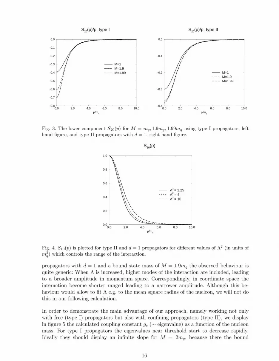
Having in mind that S2(p) describes the lower component of the nucleon Dirac field (whichis usually neglected, e.g. in nonrelativistic calculations), it is surprising that we obtainrather large “small” components. This was also observed in ref. [24]. To study this ingreater detail we plot in figure (3) the amplitude S20(p) for different values of the boundstate mass. For both types of propagators the maximum of the amplitudes S20(p) increaseswhen the binding energy EB = 2mq−M tends to 0. Note however that this result dependson the chosen representation of the fermion field (in our case the Dirac representation) 5 .We will investigate in the next section whether the large lower component of the nucleonspinor has effects on observables where a γ5 is involved in the coupling to the externalcurrent (gA(Q2) and gπNN(Q2)) because this γ-matrix induces a mixing between upperand lower components which give rise to contributions to these observables.

The dependence of the amplitudes on the width of the interaction can be seen from fig.(4). Although we restricted ourselves in the plot to a calculation of S10(p) for type II

5 We thank F. Lenz for this remark.

15

0.0 2.0 4.0 6.0 8.0 10.0p/mq

-0.8

-0.7

-0.6

-0.5

-0.4

-0.3

-0.2

-0.1

0.0

S20(p)/p, type I

M=1M=1.9M=1.99

0.0 2.0 4.0 6.0 8.0 10.0p/mq

-0.4

-0.3

-0.2

-0.1

0.0

S20(p)/p, type II

M=1M=1.9M=1.99

Fig. 3. The lower component S20(p) for M = mq, 1.9mq , 1.99mq using type I propagators, lefthand figure, and type II propagators with d = 1, right hand figure.

0.0 2.0 4.0 6.0 8.0 10.0p/mq

0.0

0.2

0.4

0.6

0.8

1.0

S10(p)

Λ2 = 2.25 Λ2

= 4 Λ2

= 10

Fig. 4. S10(p) is plotted for type II and d = 1 propagators for different values of Λ2 (in units ofm2

q) which controls the range of the interaction.

propagators with d = 1 and a bound state mass of M = 1.9mq the observed behaviour isquite generic: When Λ is increased, higher modes of the interaction are included, leadingto a broader amplitude in momentum space. Correspondingly, in coordinate space theinteraction become shorter ranged leading to a narrower amplitude. Although this be-haviour would allow to fit Λ e.g. to the mean square radius of the nucleon, we will not dothis in our following calculation.

In order to demonstrate the main advantage of our approach, namely working not onlywith free (type I) propagators but also with confining propagators (type II), we displayin figure 5 the calculated coupling constant gs (∼ eigenvalue) as a function of the nucleonmass. For type I propagators the eigenvalues near threshold start to decrease rapidly.Ideally they should display an infinite slope for M = 2mq, because there the bound

16

1.5 1.6 1.7 1.8 1.9 2.0 2.1 2.2M/mq

4.0

6.0

8.0

10.0

12.0

14.0

16.0

Eigenvalue vs. Bound State Mass

type Itype II, d=1type II, d=10

threshold ->

Fig. 5. Eigenvalues of the integral equation as functions of the bound state mass M . In case oftype I propagators, the influence of the quark-diquark threshold is clearly visible.

state decays into its constituents. To observe this feature a much more refined numericalmethod (suitable for extremely loose bound states) would be necessary. Our numericalmethod, which is very robust in a wide range of bound state masses cannot account forthis property, but signals the nearby threshold by a strong sensitivity of gs on M . Whenusing now the confining propagators we get a totally different behaviour: The eigenvaluesare not affected by the “threshold” any more (which in this case is no threshold at all).The function gs is a smooth function and nothing signals the possibility of the decayof the bound state. In this way confinement is realized in our approach: By choosingconfining propagators for the constituents of the nucleon, we exclude its unphysical decayinto free quarks and diquarks. Even when the damping factor d is increased, so that forM ≤ 1.9 the eigenvalues and eigenvectors of a type I calculation are basically recovered,near ”threshold” we again observe confinement.

Before we describe in the next section the application of the so far obtained amplitudesin a calculation of baryonic matrix elements, we want to mention that the numericalsolutions of the Bethe-Salpeter equation can be parametrized for further applicationsvery effectively. By examining the infrared and ultraviolet asymptotics of the amplitudeswe find simple rational functions with parameters fitted to the numerical solutions. Fordetails we refer to appendix B.

4 Nucleon Form Factors

In order to test the validity of the proposed quark-diquark picture of the nucleon, it isnot enough just to solve the corresponding Bethe-Salpeter equation, since its solution,the Bethe-Salpeter amplitudes (or the vertex functions) have no physical interpretationby themselves. It is therefore necessary to use the solution of the Bethe-Salpeter equa-tion to calculate physical observables as, e.g. form factors. Especially we are interested inelectromagnetic form factors of proton and neutron, the pion-nucleon form factor gπNN

17

and the axial form factor gA. These observables are accessible by coupling an appropriateprobing external current to the nucleon.In ref. [28,29] a comparable calculation to our approach was performed in the context ofthe NJL-model (with unconfined quarks and diquarks), but only static properties (vanish-ing momentum transfer) of the nucleon were considered; in ref. [30] spacelike form factorswere calulated (also within the NJL model) but assuming a static quark exchange be-tween quark and diquark and therefore working with a “trivial” nucleon vertex function.A calculation within the Salpeter approach, instead of the here employed fully relativisticBethe-Salpter equation, is reported in ref. [31] and [32]. So far, there exist no work inwhich a) the BS equation was solved without any approximation for the quark exchangeand b) the resulting solution was used to evaluate observables for finite momentum trans-fer to the nucleon. See, however, ref. [24] for a calculation of nucleon structure functionswithin this approach.At this point we make the following remarks: The so far developed picture of a nucleonconsisting of a quark and a scalar diquark with equal masses is certainly to naıve for acorrect descripton of the nucleon and therefore quantitatively agreement with experimen-tal results cannot be expected. Nevertheless we believe that the reported studies are anecessary step in the development of a complete baryon model. Therefore we not even tryto fit e.g. Λ or d to experimental numbers. Our aim is rather to observe, whether certainnucleon properties can be described reasonably.The calculation of hadronic matrix elements between bound state vertex functions is con-veniently performed in Mandelstam’s formalism [33], which will be introduced in the nextsubsection.

4.1 Mandelstam’s Formalism

In order to calculate the matrix element of an external current operator (genericallydenoted by O) between bound state amplitudes we use Mandelstam’s formalism [33] (seealso [29]), which reads in momentum space

〈O(µ)〉 = 〈N(Pf , Sf)|O(µ)|N(Pi, Si)〉 =1

√

4EPfEPi

J(µ)(Pf , Pi), (46)

J(µ)(Pf , Pi) =∫

d4pf

(2π)4

∫

d4pi

(2π)4Ψ(Pf , pf)ΓO(pf , Pf ; pi, Pi)Ψ(Pi, pi). (47)

Here Pi, pi and Pf = Pi +Q, pf denote the total and the relative momenta of the quark-diquark bound state before and after the interaction with the external current, while Ψand Ψ are the properly normalized Bethe-Salpeter wave functions. By writing explicitlythe quark and diquark propagators, which are included in the definition of the BS-wavefunction, we obtain Mandelstam’s prescription in a representation, which contains thenucleon vertex function, calculated in the previous section.

J(µ)(Pf , Pi) =∫

d4pf

(2π)4

∫

d4pi

(2π)4χ(Pf , pf)D(1

2Pf − pf)S(1

2Pf + pf) ×

ΓO(pf , Pf ; pi, Pi)D(12Pi − pi)S(1

2Pi + pi)χ(Pi, pi). (48)

18

Fig. 6. The two diagrams which contribute to the nucleon matrix elements in impulse approxi-mation.

This representation allows the direct evaluation of the nucleon current. The 5-point func-tion ΓO appearing in eq. (47) and (48) describes the coupling of the probing current withmomentum Q to the constituents of the bound state.

In the following we work in a generalized impulse approximation, where the couplingto the diquark and the constituent quark is considered, while we neglect, in this firstcalculation, the coupling to the exchanged quark.Accordingly the 5-point function is defined by

ΓO(pf , Pf ; pi, Pi) = δ(pf − pi − 12Q)D−1(1

2Pi − pi)Γ

q

O(pf , Pf ; pi, Pi)

+δ(pf − pi + 12Q)S−1(1

2Pi + pi)Γ

dO(pf , Pf ; pi, Pi). (49)

Inserting ΓO into eq. (48), one observes that the matrix element is split into a quark anda diquark part

J(µ)(Q2) = Jq

(µ)(Q2) + Jd

(µ)(Q2). (50)

If the external nucleon legs are on their mass shells (P 2i = P 2

f = −M2), the nucleoncurrent depends only on the squared momentum Q2 of the probing external current. Thetwo terms appearing in (50) are given by the loop integrals

Jq(µ)(Q

2) =∫

d4p

(2π)4χ(Pf , pf)S(p+)Γq

(µ)(p+, p−)S(p−)D(pd)χ(Pi, pi), (51)

and

Jd(µ)(Q

2) =∫

d4p

(2π)4χ(Pf , pf)D(p+)Γd

(µ)(p+, p−)D(p−)S(pq)χ(Pi, pi). (52)

In appendix C we discuss the momentum rooting in the loop integrals and their numericalevaluation.Since the Bethe-Salpeter equation does not provide the overall normalization of the boundstate vertex function, a physical normalization condition has to be imposed. The usualrequirement, a unit residue of the bound state propagator at the mass pole [34], which in

19

our formalism reads

∫

d4p

(2π)4χ(P, p)[

∂

∂Pµ

S(12P + p)D(1

2P − p)]χ(P, p) = 2Λ+P µ, (53)

then leads to the correct normalization. Since the quark exchange is independent of thec.m. momentum P , it does not contribute to the normalization of the vertex function.Note that the adjoint vertex function χ(P, p) has to fulfill

χ(P, p) = Λ+χ(P, p) (54)

and is therefore given by χ(P, p) = γ4χ†(P, p)γ4.

4.2 Electromagnetic Form Factors

To determine the electromagnetic (e.m.) form factors one has to calculate the e.m. nu-cleon current. The probing current is an external photon and therefore the quark-photonand the diquark-photon vertex functions are needed to apply Mandelstam’s formalism.Electromagnetic gauge invariance is manifest in the Ward-Takahashi identity,

QµΓµ(p+Q, p) = S−1(p+Q) − S−1(p), (55)

which provides the connection between the longitudinal part of the (di-)quark-photonvertexfunction and the inverse (di-)quark propagator, and for the limit Q2 → 0 in theWard identity

Γµ(p, p) =∂

∂pµS−1(p). (56)

Using vertex functions in accordance with these identities means to respect gauge invari-ance at the constituent level.A vertex function which solves the above identites for the quark-photon coupling is theBall-Chiu vertex [35,36],

(Γqµ)e.m.(p, k) = ΓBC

µ (p, k) = iA(p2) + A(k2)

2γµ

+ i(p+ k)µ

p2 − k2

[

(A(p2) − A(k2))γp+ γk

2− i(B(p2) − B(k2))

]

, (57)

which is determined by the quark self-energy functions A(p2) and B(p2) appearing in thequark propagator

S(p) = −iγ ·pσv(p2) + σs(p

2) = [iγ ·pA(p2) +B(p2)]−1 (58)

and can be read off from eq. (3). The vertex function (57) not only satisfies eqs. (55) and(56), but is also free of kinematical singularities, has the same properties under P,C,Ttransformations as the perturbative vertex iγµ and reduces itself to this vertex in case of

20

bare quarks (this is the case when a type I quark propagator is used). In the following wewill restrict ourselves to the pure longitudinal Ball-Chiu vertex and will not consider anytransversal part, which cannot be determined using e.m. gauge invariance 6 .The vertex function of a nonperturbative (extended) scalar particle, also has to be chosento fulfill eqs. (55) and (56); this is discussed in ref. [38]. Again we will use the simplestlongitudinal diquark-photon vertexfunction

(Γdµ)e.m.(p, k) = −(p+ k)µ

[

p2C(p2) − k2C(k2)

p2 − k2−ms

C(p2) − C(k2)

p2 − k2

]

(59)

which is determined by the self-energy function C(p2) of the diquark propagator

D(p) = − F (p2)

p2 +m2s

= −(

(p2 +m2s)C(p2)

)−1. (60)

The explicit expression can be easily obtained when comparing with eq. (4). In particular,any transversal part of the vertex function, which would describe an anomalous magneticmoment of the scalar diquark will not be considered.To calculate the electromagnetic form factors of the nucleon we insert

Γqµ(p+, p−) = Qq(Γ

qµ)e.m.(p+, p−) (61)

and

Γdµ(p+, p−) = Qd(Γ

dµ)e.m.(p+, p−) (62)

with the charge matrices in isospin space given by

Qq = 12(1

31 + τ z), Qd = 1

3. (63)

into eqs. (51) and (52), respectively, and evaluate the loop integrals. As it is well known,using Lorentz invariance, invariance under P,C,T and the fact that the incoming andoutgoing nucleons are onshell, the longitudinal e.m. nucleon current can be decomposedinto

Je.m.µ (Q2) = Λ+(Pf , Sf )[iMB(Fe(Q

2) − Fm(Q2))Pµ

P 2+ Fm(Q2)γµ]Λ

+(Pi, Si).

(64)

Note that within our formalism the Dirac spinors usually appearing on the right handside of this equation are replaced by the Λ+ projectors. The Lorentz invariant functionsFe(Q

2) and Fm(Q2) denote the electric and magnetic form factor, which can be extractedby taking appropriate traces. Here and in the following subsections the calculations aremost conveniently performed in the Breit-frame (see appendix C).

6 In ref. [37] it was shown that the requirement of multiplicative renormalisibility constrainsthe construction of possible transversal parts of the e.m. vertexfunction.

21

4.3 Pion Nucleon Form Factor

The pion nucleon form factor, which enters into pure hadronic models usually as an inputparameter, has been much debated in the last few years. Especially the value at the pionmass shell is not directly accessible in experiments. For a recent analysis obtained fromdifferent experiments (πN scattering, NN scattering, ...) see ref. [39]. In this respect thereis certainly the need to calculate this observable from a more fundamental quark level.Within our approach the pion nucleon form factor is obtained by coupling an external pioncurrent to the diquark-quark bound state using again Mandelstam’s formalism. Becauseof parity conservation one notes that there is no contribution from the loop integral(52) where the pion would couple to the 0+ diquark. So the relevant nucleon current iscompletely carried by the quark part (51). In order to specify the vertex function forthe pion-quark coupling we use spontaneously broken chiral symmetry and Goldstone’stheorem [40]: In the chiral limit the vertex function, which is nothing else than the pionBethe-Salpeter amplitude, is proportional to the scalar self energy of the quark. This isa consequence of the fact that in the chiral limit (vanishing quark current mass) where,provided the pion mass vanishes (Goldstone’s theorem), the pion Bethe-Salpeter equationis equivalent to the quark Dyson-Schwinger equation. Therefore the proper choice is

Γaπ(P 2

π = Q2 = 0, p2) = iγ5B(p2)

fπ

τa, (65)

where B(p2) is defined in eq. (58) and the experimental pion decay constant fπ = 0.093GeV is used. Although this choice of the pion-quark vertex is valid only at the pion massshell Q2 = 0, we assume that the offshell amplitude does not vary too much with the pionmomentum and therefore the most obvious generalization [41]

Γaπ(Q2, p2) = iγ5

τa

2

1

fπ(B((p− 1

2Q)2) +B((p+ 1

2Q)2)) (66)

of the onshell vertex function is allowed at least for a few hundert MeV around the onshellpoint.When inserting the pion quark vertex function into eq. (51) and evaluating the loopintegral we determine the pion-nucleon form factor. Furthermore since the pion-nucleonmatrix element is parametrized as

Jπ(Q2) = 〈N(Pf , Sf)|jπ(Q2)|N(Pi, Si)〉= Λ+(Pf , Sf)[γ5gπNN(Q2)τa]Λ+(Pi, Si). (67)

the extraction of gπNN(Q2) is straightforward.

4.4 Axial Form Factor

Finally we calculate the axial form factor gA(Q2) of the nucleon. Due to parity, we againhave to consider only the quark part of the nucleon current, since an axial current does

22

not couple to the scalar diquark. To specify the relevant vertex function, where the axialcurrent interacts with the quark, we use the chiral Ward identity which reads

QµΓ5µ(p+Q, p) = S−1(p+Q)γ5 − γ5S−1(p). (68)

This symmetry constraint can be satisfied with the vertex [40]

Γa5µ(p, k) =

(

iA(p2) + A(k2)

2γµ

+ i(p+ k)µ

p2 − k2

[

(A(p2) − A(k2))γp+ γk

2− i(B(p2) +B(k2))

])

γ5τa

2, (69)

that is totally determined by the quark self-energies. Although the axialvector vertexfunction looks, up to the isospin generators and the explicit γ5, very similar to the Ball-Chiu vertex (57) (used in the case of a vector current coupling), there is one importantdifference: In the last term the scalar quark self-energies B(p2) and B(k2) add up, whichin the limit Q = p− k → 0 leads to

QµΓa5µ(p, k) −→ τaB(p2)γ5. (70)

When comparing (70) with eq. (65), the pion-quark vertex, one observes the exact Gold-berger Treiman relation for the quarks in the chiral limit:

limQ→0

iQµΓa5µ(p, k) = fπΓa

π(0, p2). (71)

Stated in other words, in the chiral limit the axialvector quark coupling for vanishingmomentum transfer is completely dominated by the pseudoscalar coupling to a masslesspion (conserved axial current).To examine whether the phenomenologically much more important Goldberger-Treimanrelation on the nucleon level

gπNN = gAM

fπ

(72)

is fulfilled, we have to determine gA(Q2) by taking the matrix element of the axial currentbetween the diquark-quark bound states. After using the axialvector vertex function (69)to evaluate (51) and comparing the result with the familiar decomposition

Jaµ(Q2) = 〈N(Pf , Sf)|ja

µ(Q2)|N(Pi, S)〉

= Λ+(Pf , Sf)τa

2[γµgA(Q2) +QµgP (Q2)]γ5Λ

+(Pi, Si)

(73)

of the matrix element, the invariant form factors are immediately accessible. Note thatbesides gA(Q2), the axial form factor of the nucleon, there exist another form factorgP (Q2), the induced pseudoscalar form factor with a pole at the pion mass shell.

23

4.5 Discussion of Numerical Results

In this subsection we finally show and discuss our results for the nucleon form factors.We will concentrate again on three different cases: Using type I propagators, the solutionof the corresponding Bethe-Salpeter equation and the appropriate vertex functions; usingtype II propagators with d = 1 and with d = 10. The so obtained electromagnetic formfactors of the nucleon are shown in fig. (7).

0.0 0.2 0.4 0.6 0.8 1.0 1.2 1.4 1.6 1.8 2.0Q

2/GeV

2

0.0

0.2

0.4

0.6

0.8

1.0

Fe

P(Q

2)

type Itype II, d=1type II, d=10Dipol

0.0 0.2 0.4 0.6 0.8 1.0 1.2 1.4 1.6 1.8 2.0Q

2/GeV

2

-0.1

0.0

0.1

0.2

0.3

0.4

Fe

N(Q

2)

type Itype II, d=1type II, d=10

0.0 0.2 0.4 0.6 0.8 1.0 1.2 1.4 1.6 1.8 2.0Q

2/GeV

2

0.0

0.2

0.4

0.6

0.8

1.0

1.2

1.4

1.6

1.8

Fm

P(Q

2)

type Itype II, d=1type II, d=10

0.0 0.2 0.4 0.6 0.8 1.0 1.2 1.4 1.6 1.8 2.0Q

2/GeV

2

-0.8

-0.7

-0.6

-0.5

-0.4

-0.3

-0.2

-0.1

0.0

Fm

N(Q

2)

Typ Itype II, d=1type II, d=10

Fig. 7. Electromagnetic form factors of the nucleon.The nucleon mass in all cases is chosen tobe M = 1.9mq and the amplitudes entering the calculation of the matrix elements are obtainedwith Λ = 2mq.

First of all, we mention (as can also be seen in the figures), that it is not possible ingeneral to obtain exact charge conservation. This is due to the impulse approximation,where the coupling of the photon to the exchanged quark (and also to the diquark-quarkform factor) is neglected. Whereas in a Salpeter approach charge conservation can be

24

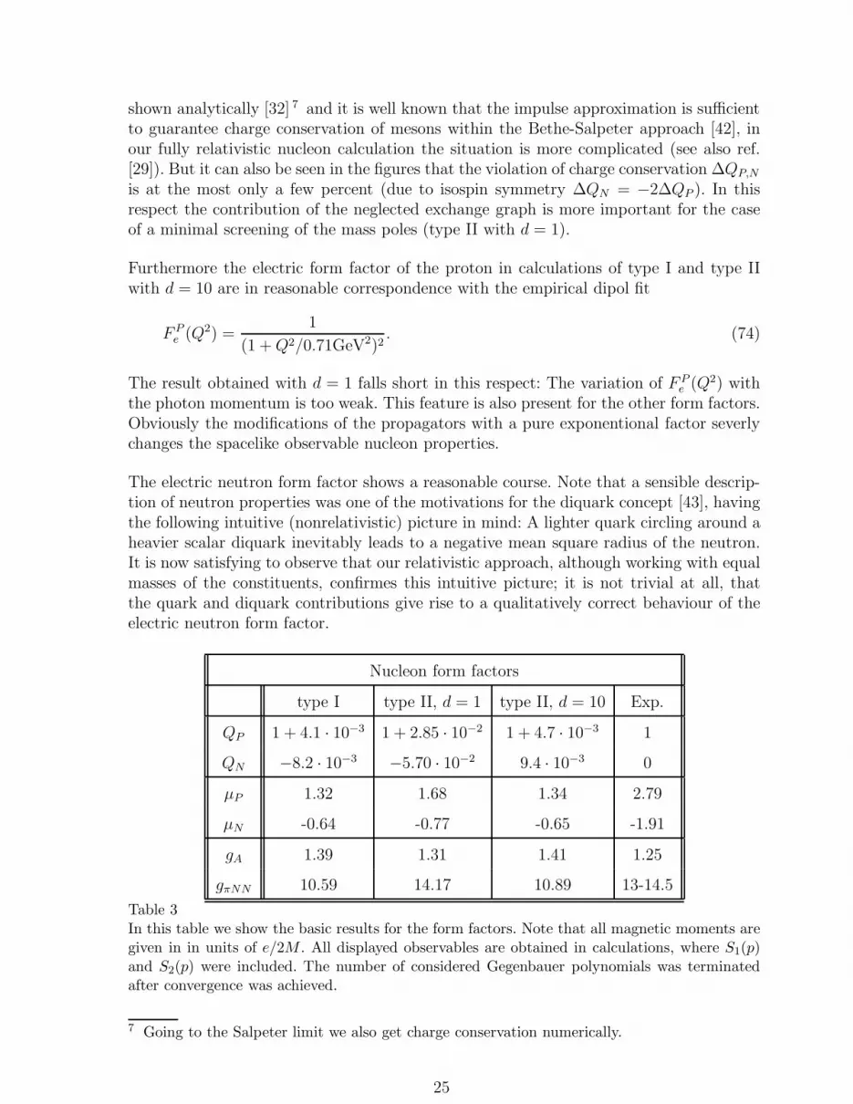
shown analytically [32] 7 and it is well known that the impulse approximation is sufficientto guarantee charge conservation of mesons within the Bethe-Salpeter approach [42], inour fully relativistic nucleon calculation the situation is more complicated (see also ref.[29]). But it can also be seen in the figures that the violation of charge conservation ∆QP,N

is at the most only a few percent (due to isospin symmetry ∆QN = −2∆QP ). In thisrespect the contribution of the neglected exchange graph is more important for the caseof a minimal screening of the mass poles (type II with d = 1).

Furthermore the electric form factor of the proton in calculations of type I and type IIwith d = 10 are in reasonable correspondence with the empirical dipol fit

F Pe (Q2) =

1

(1 +Q2/0.71GeV2)2. (74)

The result obtained with d = 1 falls short in this respect: The variation of F Pe (Q2) with

the photon momentum is too weak. This feature is also present for the other form factors.Obviously the modifications of the propagators with a pure exponentional factor severlychanges the spacelike observable nucleon properties.

The electric neutron form factor shows a reasonable course. Note that a sensible descrip-tion of neutron properties was one of the motivations for the diquark concept [43], havingthe following intuitive (nonrelativistic) picture in mind: A lighter quark circling around aheavier scalar diquark inevitably leads to a negative mean square radius of the neutron.It is now satisfying to observe that our relativistic approach, although working with equalmasses of the constituents, confirmes this intuitive picture; it is not trivial at all, thatthe quark and diquark contributions give rise to a qualitatively correct behaviour of theelectric neutron form factor.

Nucleon form factors

type I type II, d = 1 type II, d = 10 Exp.

QP 1 + 4.1 · 10−3 1 + 2.85 · 10−2 1 + 4.7 · 10−3 1

QN −8.2 · 10−3 −5.70 · 10−2 9.4 · 10−3 0

µP 1.32 1.68 1.34 2.79

µN -0.64 -0.77 -0.65 -1.91

gA 1.39 1.31 1.41 1.25

gπNN 10.59 14.17 10.89 13-14.5

Table 3In this table we show the basic results for the form factors. Note that all magnetic moments aregiven in in units of e/2M . All displayed observables are obtained in calculations, where S1(p)and S2(p) were included. The number of considered Gegenbauer polynomials was terminatedafter convergence was achieved.

7 Going to the Salpeter limit we also get charge conservation numerically.

25

0.0 0.2 0.4 0.6 0.8 1.0 1.2 1.4 1.6 1.8 2.0Q

2/GeV

2

0.0

0.2

0.4

0.6

0.8

1.0

1.2

1.4

Axial form factor gA(Q2)

type Itype II, d=1type II, d=10

0.0 0.2 0.4 0.6 0.8 1.0 1.2 1.4 1.6 1.8 2.0Q

2/GeV

2

0.0

2.0

4.0

6.0

8.0

10.0

12.0

14.0

Pion nucleon form factor gπNN(Q2)

type Itype II, d=1type II, d=10

Fig. 8. The axial form factor gA(Q2) of the nucleon and the pion nucleon form factor gπNN (Q2)are shown for type I and type II with d = 1, 10 calculations respectively.

0.0 0.2 0.4 0.6 0.8 1.0 1.2 1.4 1.6 1.8 2.0Q

2/GeV

2

0.0

0.2

0.4

0.6

0.8

1.0

1.2

1.4

Axial form factor gA(Q2)

type II, d=10

S1 and S2

S1

0.0 0.2 0.4 0.6 0.8 1.0 1.2 1.4 1.6 1.8 2.0Q

2/GeV

2

0.0

2.0

4.0

6.0

8.0

10.0

12.0

14.0

Pion nucleon form factor gπNN(Q2)

type II, d=10

S1 and S2

S1

Fig. 9. The axial form factor gA(Q2) and the pion nucleon form factor gπNN (Q2) are shown fora type II with d = 10 calculation, including only S1(p) or including S1(p)and S2(p).

For both proton and neutron, the magnetic moments are too small. This is, however, notsurprising because large contributions coming from 1+ diquarks are expected for theseobservables ([32], [44]). Nevertheless, the calculated values have magnitudes expectedfrom a calculation involving only 0+ diquarks [30,31].

Before discussing the axial properties of the nucleon, we mention the following behaviourof the form factors: When Λ is decreased, leading to narrower amplitudes in momentumspace (compare fig. (4)), the electric form factors for the type I calculation become steeperand approach the emperical dipol fit. While such a behaviour is expected near threshold[45] we do not observe this feature for type II calculations. In these calculations the formfactors (at leat at small Q2) are very insensitive on Λ and the actual value of the bound

26

state mass.

Our results for the axial and the pion-nucleon form factor are shown in fig. (8). Again,we observe for a type II with d = 1 calculation a relatively small variation of the formfactors with Q2. Furthermore for the calculation including type II propagators with d = 10the similarities to the type I case can be seen. A striking feature, however, is the goodagreement of gA = gA(Q2 = 0) and gπNN = gπNN(Q2 = 0) with the experimental values.gA tends to be slightly too large whereas the pion nucleon coupling constant obtainedwith type I and with type II (d=10) is a little bit too small. Nevertheless, in all casesa qualitatively right behaviour is obtained. This is astonishing, because also for theseobservables (in analogy to the magnetic moments) sizeable contributions from 1+ diquarksare expected. Note that in ref. [29] also a relatively large value of gA has been obtained,including only 0+ diquarks.

By comparing the calculated values of gπNN with the ones obtained form the GoldbergerTreiman relation (72) we observe a violation of the Goldberger Treiman relation up to 30%.This failure also signals the necessity for the inclusion of 1+ diquarks in the calculation. Itis furthermore to be seen how much the exchanged quark contributes to these observables.

In figure (9) we show the influence of the lower component S2(p) of the nucleon Diracfield by comparing the results obtained with all amplitudes with the result obtained withS1(p) alone. It is interesting to note that the values of gπNN(Q2) at small values of themomentum transfer are influenced by S2(p); while the values of gA(Q2) at larger valuesare slightly more affected. Nevertheless we conclude that having a large lower componentis probably only due to the representation chosen for the Dirac matrices. They do nothave a significant effect on observables studied so far.

5 Conclusions and Outlook

In this paper we have developed a covariant diquark-quark model suitable for the calcu-lation of nucleon observables. As discussed, confinement is put in by a modification ofthe free (tree-level) quark and diquark propagators. The structure of the Bethe-Salpeterequation, describing nucleons as diquark-quark bound states interacting through quarkexchange, has been elaborated using an appropriate decomposition of the Bethe-Salpetervertex function in the Dirac algebra. Furthermore, the coefficient functions of the cor-responding Lorentz tensors have been expanded in hyperspherical harmonics, exploitingan approximate O(4) symmetry (which would be exact if the exchanged particle weremassless). After discussing the various numerical methods we presented our results forthe calculation including 0+ diquarks. The advantages of the confining propagators areclearly seen in the absence of unphysical thresholds.

The numerically obtained nucleon vertex function has been fitted to a simple analyticform and then used to calculate nucleon matrix elements and form factors. In particular,we considered electromagnetic, the axial and the pionic form factors of the nucleon. While,due to the various simplifications and approximations, a quantitative agreement of the

27

results with experimental values could not be expected, we nevertheless got reasonableresults. Furthermore, the large lower component of the nucleon Dirac field was shown to bemerely an artefact of the chosen spinor representation. Although, the various observablesdisplayed that the developed picture of a nucleon is still oversimplified, they neverthelessgive us confidence that we are on the right track in obtaining a reasonable and trustablebaryon model. The next step of improvement will be the inclusion of 1+ diquarks in theBethe-Salpeter equation and also in the nucleon matrix elements. Furthermore we planto determine the internal structure of the diquarks (described crudely by the parameterΛ) by a microscopic diquark model.

In order to fully exploit the advantages and possibilities of our covariant and confining ap-proach, the model will soon be applied to other processes. In particular, we will investigatethe different observables associated with the reactions p+γ → K +Λ and p+ p→ K +Λwhich are measured at ELSA [46] and COSY [47], respectively.While in most calculations of nucleon structure functions the distribution functions of theconstituents are merely parametrized (see e.g. [48]), our approach offers the possibility todetermine, in a first step, these distributions, after the constituents are specified. In ref.[24] this was investigated, assuming the scalar diquark to be a spectator and the photoninteracts only with the quark.

We conclude, that the reported studies are a good starting point for further investigations,which certainly will improve our qualitative and quantitative understanding of the baryonstructure.

Acknowledgments We thank Rolf Baurle and Udo Zuckert for their contributions inthe early stages of this work, and G. Piller and K. Kusaka for the very helpful discussionson the numerical solution of the Bethe-Salpeter equation. Helpful remarks by F. Lenz aregratefully acknowleged.

A Dirac Decomposition

We choose the following ansatz for the amplitude χµ

χµ(P, p) = A1(P, p)γ5PµΞΛ+ + A2(P, p)γ5P

µΛ+

+ B1(P, p)γ5pµT ΞΛ+ + B2(P, p)γ5p

µT Λ+

+ C1(P, p)γ5i(Pµ1 − γµ)Λ+ + C2(P, p)γ5i(P

µ1 + γµ)ΞΛ+ (A.1)

In the rest frame of the bound state, P = (0, 0, 0, iM), we obtain by using

Λ+ =(

1 00 0

)

, ΞΛ+ =(

0 0pσ 0

)

. (A.2)

the following expressions:

χ4 =(

pσA1(P, p) 01A2(P, p) 0

)

(A.3)

28

and

χ =(

(pσ)pB1(P, p) 0pB2(P, p) 0

)

+(

σC1(P, p) 0σ(pσ)C2(P, p) 0

)

(A.4)

Using the redefinitions

Bi = Bi − Ci, Ci = Ci

turns eq. (A.1) into eq. (21). In the rest frame this leads to

χ =(

p(pσ)B1(P, p) + i(σ × p)(pσ)C1(P, p) 0pB2(P, p) + i(σ × p)C2(P, p) 0

)

(A.5)

Thus in the rest frame the meaning of the amplitudes is therefore as follows: the am-plitudes Ai are the time components, the components Bi are parallel to the relativethree–momentum of the constituents, and the components in the third line in eq. (21) areorthogonal to the momentum and the spin.

B Analytic fits of the amplitudes

0.0 2.0 4.0 6.0 8.0 10.0p/mq

0e+00

2e-05

4e-05

6e-05

8e-05

1e-04

Fit Quality of S10(p)

Fig. B.1. (S10(p)numeric − S10(p)fit)2 is plotted for the type II calculation with M = 1.9mq .

After solving the Bethe-Salpeter equation the amplitudes S10(p) ... S22(p) are given onlyat the grid points of the momentum mesh. For further use in the calculation of matrixelements this a very unconvenient feature. Therefore we fit rational funtions to them. To dothis the value of every amplitude at each grid point is therefore treated as a “data” pointwith a certain standart deviation σ. We find that the following set of rational functionsare suitable to take the behaviour at small p as well as the behaviour at large p properly

29

Fit coefficients for type I

S10 S11 S12 S20 S21 S22

a1 0.9992 -0.6954 0.03028 -0.4191 0.4113 -0.0127

b1 0.3107 0.3028 0.4617 0.2682 0.1937 0.4090

a2 -0.0002 0.2929 0.0134 -0.1841 -0.3939 -0.0058

b2 7.8284 0.3028 0.1834 0.0792 0.1966 0.2085

χ2σ 6.786 · 10−5 4.025 · 10−5 9.474 · 10−9 1.132 · 10−5 2.347 · 10−8 1.207 · 10−10

Table B.1The fit coefficients for a type I calculation with M = mq and Λ = 2mq are displayed.

Fit coefficients for type II, d = 1

S10 S11 S12 S20 S21 S22

a1 1.6562 -0.9674 0.4988 -0.4168 0.3898 0.5042

b1 0.2437 0.2556 0.1985 0.0924 0.1564 0.1562

a2 -0.6574 0.6342 -0.4686 0.0463 -0.3528 -0.5069

b2 0.3838 0.3293 0.2046 0.0924 0.1613 0.1558

χ2σ 5.305 · 10−4 1.340 · 10−4 5.331 · 10−7 1.035 · 10−4 5.263 · 10−8 3.594 · 10−9

Table B.2The fit coefficients for a type II calculation with d = 1, M = mq and Λ = 2mq are displayed.

into account :

S10(p) =2∑

k=1

ak10

(1 + bk10p2)2

(B.1)

S11(p) =2∑

k=1

ak11p

(1 + bk11p2)2

(B.2)

S12(p) =2∑

k=1

ak12p

2

(1 + bk12p2)3

(B.3)

S20(p) =2∑

k=1

ak20

(1 + bk20p2)3

(B.4)

S21(p) =2∑

k=1

ak21p

2

(1 + bk21p2)3

(B.5)

S22(p) =2∑

k=1

ak22p

3

(1 + bk22p2)4

(B.6)

(B.7)

30

Note, that the momentum p is taken in units of the quark mass. The fit coefficientsak

ij , bkij ; i, j = 1, 2; k = 1, 2 are then determined independently for each amplitude by

performing a χ2 fit. To judge the quality of this procedure we show in fig. (B.1) thesquared deviation

∆2 = (S10(p)numeric − S10(p)fit)2. (B.8)

Suming up the squared deviations then leads to

σ2χ2 =kmax∑

k=1

∆2 =kmax∑

k=1

(S10(k)numeric − S10(k)fit)2, (B.9)

i.e. the merit function χ2 times the squared accuracy of the “data points”. In the tables(B.1) and (B.2) we show the fit coefficients which reproduce the plots for the type I andthe type II with d = 1 amplitudes given in figure (2) within very small deviations.

C Evaluation of the loop integrals

In Section 4.1 we derived the two loop integrals building up the nucleon current. In eq.(51)

Jqµ(Q2) =

∫

d4p

(2π)4χ(Pf , pf)S(p+)Γq

µ(p+, p−)S(p−)D(pd)χ(Pi, pi), (C.1)

the momenta are definded as

p± = p+ 12Pi + 1

2Q± 1

2Q

pd = −p + 12Pi (C.2)

whereas in eq. (52)

Jdµ(Q2) =

∫

d4p

(2π)4χ(Pf , pf)D(p+)Γd

µ(p+, p−)D(p−)S(pq)χ(Pi, pi). (C.3)

the momenta are chosen as

p± = −p + 12Pi + 1

2Q± 1

2Q

pq = p+ 12Pi. (C.4)

As stated in the text, to evaluate these integrals it is useful to work in the Breit-frame

Q = (0, 0, Q3, 0)

Pi = (0, 0,−12Q3, i

√

M2 + 14Q2)

Pf = (0, 0, 12Q3, i

√

M2 + 14Q2), (C.5)

31

and further to express the loop momentum p in 4-dimensional spherical coordinates

p = p (sinφ sin θ cosψ, sinφ sin θ sinψ, sinψ cos θ, cosψ) . (C.6)

While the φ integration is trivial, the integration over p, Θ and ψ has to be performednumerically.

References

[1] Procceedings of the Conference Diquarks 3, Torino, Oct. 28-30,1996; eds.: M. Anselminoand E. Predazzi, to be published by World Scientific.

[2] R. T. Cahill, Austr. J. Phys. 42, 171 (1989).

[3] H. Reinhardt, Phys. Lett. B244, 316 (1990).

[4] M. G. Olsson, e-print hep-ph/9702213.

[5] P. Hasenfratz and J. Kuti, Phys. Rep. 40, 75 (1978).

[6] T. H. R. Skyrme, Proc. Roy. Soc. A260, 127 (1961);see also: G. S. Adkins, C. R. Nappi, and E. Witten, Nucl. Phys. B228, 552 (1983);G. Holzwarth (Ed.), Baryons as Skyrme Solitons (World Scientific Publ. Comp., Singapore,1993).

[7] R. Alkofer, H. Reinhardt, and H. Weigel, Phys. Rep. 265, 139 (1996);C. V. Christov et al., Prog. Part. Nucl. Phys. 37, 1 (1996).

[8] M. Gell-Mann, Phys. Rev. 8, 214 (1964).

[9] G. Karl and E. Obryk, Nucl. Phys. B8, 609 (1968).

[10] D. Faiman and A. W. Hendry, Phys. Rev. 173, 1720 (1968).

[11] L. Ya. Glozman, Z. Papp, W. Plessas, K. Varga and R. F. Wagenbrunn,e-print nucl-th/9705011.

[12] R. P. Feynman, M. Kislinger, and F. Ravndal, Phys. Rev. D3, 2706 (1971).

[13] A. Chodos and C. Thorn, Phys. Rev. D12, 2733 (1975).

[14] M. Rho, Phys. Rep. 240, 1 (1994).

[15] Y. Nambu and G. Jona-Lasinio, Phys. Rev. 122, 345 (1961).

[16] U. Zuckert, R. Alkofer, H. Weigel, and H. Reinhardt, Phys. Lett. B362, 1 (1995);Phys. Rev. C55, 2030 (1997).

[17] H. J. Munczek and A. M. Nemirovsky, Phys. Rev. D 28, 181 (1983).

[18] D. Ebert, T. Feldmann and H. Reinhardt, Phys. Lett. B388, 154 (1996).

[19] A. Bender, C. D. Roberts, and L. v. Smekal, Phys. Lett. B380, 7 (1996).

32

[20] P. Jain and H. J. Munczek, Phys. Rev. D 48 (1993) 5403.

[21] A. Buck, R. Alkofer, and H. Reinhardt, Phys. Lett. B286, 29 (1992);A. Buck and H. Reinhardt, Phys. Lett. B356, 168 (1995).

[22] C. Hanhart and S. Krewald, Phys. Lett. B344, 55 (1995).

[23] G. Hellstern, R. Alkofer and H. Reinhardt, in preparation.

[24] K. Kusaka, G. Piller, A. W. Thomas, A. G. Williams, e-print hep-ph/9609277, to bepublished in Phys. Rev. (1997).

[25] H. Meyer, Phys. Lett. B337, 37 (1994).

[26] M. Abramowitz and I. A. Stegun, Handbook of Mathematical Functions, Dover, New York,1965.

[27] V. Keiner, Z. Phys. A354, 87 (1996).

[28] N. Ishii, W. Bentz, and K. Yazaki, Nucl. Phys. A587, 617 (1995).

[29] H. Asami, N. Ishii, W. Bentz and K. Yazaki, Phys. Rev. C 52, 3388 (1996).

[30] G. Hellstern, C. Weiss, Phys. Lett. B 351 64 (1995).

[31] V. Keiner, Z. Phys. A354, 87 (1996).

[32] V. Keiner, Phys. Rev. C 54, (1996) 3232;PhD Thesis, University of Bonn 1997, http://pythia.itkp.uni-bonn.de/bspub.html.

[33] S. Mandelstam, Proc. Roy. Soc. 233 248 (1955).

[34] C. Itzykson, J.-B. Zuber: Quantum Field Theory, McGraw–Hill (1985).

[35] J. S. Ball and T.W. Chiu, Phys. Rev. D 22 2542 (1980).

[36] D. Kusno, Phys. Rev. D 27 1657 (1983).

[37] D. C. Curtis and M. R. Pennington, Phys. Rev. D46 2663 (1992).

[38] K. Ohta, Phys. Rev. C 41 1213 (1990).

[39] T. E. O. Ericson, Nucl. Phys. A 543 409c (1993);T. E. O. Ericson and B. Loiseau, hep-ph/9612420.

[40] R. Delbourgo, M. D. Scadron, J. Phys. G 5 (1979) 1621.

[41] C. D. Roberts, A. G. Williams, Prog. Part. Nuc. Phys. 33 (1994).

[42] C. D. Roberts, Nucl. Phys. A 605 (1996) 475.

[43] Z. Dziembowski, W. J. Metzger and R. T. Van de Walle, Z. Phys. C 10 231 (1981).

[44] C. Weiss, A. Buck, R. Alkofer and H. Reinhardt, Phys. Lett. B 312 (1993) 6.

[45] R. L. Jaffe, P. F. Mende, Nucl. Phys. B369 (1992) 189.

[46] M. Bockhorst et. al. (SAPHIR), Z. Phys. C63, (1994) 37.

[47] W. Eyrich, private communication.

[48] R. Jakob, P. J. Mulders and J. Rodrigues, e-print hep-ph/9704335.

33