Numerical multiscale methods

A.L.G.A. CoutinhoCenter for Parallel Computing and Department of Civil Engineering

COPPE/Federal University of Rio de JaneiroP.O. Box 68506

Rio de Janeiro, RJ 21945, Brazil

L. P. FrancaUniversity of Colorado Denver

Department of Mathematical and Statistical SciencesP.O.Box 173364, Campus Box 170

Denver, Colorado 80217-3364

F. ValentinNational Laboratory for Scientific Computing - LNCC

Av. Getúlio Vargas, 33325651-070 Petrópolis, RJ, Brazil

Abstract

We restrict the Variational Multiscale Method to a class of methods we denote by Numerical Multiscale Methods.Numerical multiscale methods are methods obtained by enriching the piecewise linear functions with special localfunctions. The enrichment provides additional stabilization via terms obtained by static condensation. The resultingmethods are improvements of the coarse scale solutions by the approximations of the fine scales emanating from theenrichments.

1 IntroductionIn the Variational Multiscale Method [15] the solution to a problem is decomposed as follows:

u = u + u′ ,

where u represents coarse scales and u′ represents fine scales. The decomposition is pretty general and its physicalinterpretation comes from turbulence.

When we make u spanned by the standard piecewise linear finite element space and we make u′ spanned by specialfunctions with local support we have the decomposition of a Numerical Multiscale Method:

u = u1 + ue .

The early studies of special functions includes bubbles and residual-free bubbles [2, 4] and their developmentpreceded the development of the Variational Multiscale Method.

Numerical Multiscale Methods are closely related to stabilized methods. Stabilized methods [5, 8, 7] offer stabilityand convergence features to coarse meshes. They are examples of coarse mesh high accurate methods. These featuresallow simulations with reasonable computing resources. Besides, compatibility restrictions are circumvented usingstabilized methods [16].

To derive stabilized methods we use the principle of enriching lower order polynomials using the standard Galerkinmethod. We start by adding bubble functions to piecewise linears for the advective-diffusive model. We show that thisGalerkin method is equivalent to SUPG with special stabilization parameter produced by the bubble shape functions[2]. The method can be seen as an approximation to the fine scales by the bubble functions. Their effect produces animproved numerical method to the coarse scales. This is an example of a Numerical Multiscale Method. See [18] foran application to the Navier-Stokes equation.

1

Next we present a special class of bubble functions, the so-called residual-free bubble functions [4, 14]. They areobtained by enforcing the bubble part of the solution to satisfy strongly the partial differential equations. We illustratethe method for the advective-diffusive equation.

The solution at element-level of the residual-free bubble functions can be complex. In these cases we approximatethem by a two-level method [9, 12, 13] consisting in solving the partial differential equations by a suitable finiteelement method at the element level. We illustrate this approach with the advective diffusive equation.

The drawback of bubble functions is the enforcement of zero boundary conditions. This can be unacceptable tocertain equations such as the reaction-diffusive equation when the reaction coefficient is much larger than the diffusiveone. To relax the zero boundary constraint, we first consider the Discontinuous Enrichment Method (DEM) withLagrange multipliers to enforce continuity of the discontinuous enrichment functions [6]. Next, we present the Petrov-Galerkin Enrichment Method (PGEM) consisting in enriching the piecewise functions with functions that may notequal to zero in the boundary [11, 10, 1]. The resulting method can be equally seen as a multicale approach wherethe interior functions are approximations to the fine scales that improve the overall method for the coarse scales. Theresulting method is a stabilized-like method.

We conclude the paper with some remarks.

2 Advective-diffusive equationWe illustrate the methods discussed herein with the advective-diffusive model. We wish to find the scalar function usuch that

−κ∆u + a · ∇u = f inΩ ⊂ R2 ,

where Ω is the open bounded domain, κ is the positive constant diffusivity coefficient, a is the velocity field, assumedto be constant in each element, f is a given source, also assumed to be constant in each element.

For simplicity, consider:u = 0 onΓ = ∂Ω .

The corresponding variational formulation is: Find u ∈ H10 (Ω) such that

κ(∇u,∇v) + (a · ∇u, v) = (f, v) ∀v ∈ H10 (Ω) ,

where the space H10 (Ω) and the inner-product (., .) have standard meaning.

To define the Galerkin method we partition the domain into triangles or quadrilaterals and define functions on eachelement that span a space Vh such that:

Vh ⊂ H10 (Ω) .

Then, the Galerkin method is: Find uh ∈ Vh such that

κ(∇uh,∇v) + (a · ∇uh, v) = (f, v) ∀v ∈ Vh .

The standard choice of Vh is to use the space spanned by continuous piecewise linear or bilinear (isoparametric)polynomials, denoted by V1.

Nevertheless, the methodology presents numerical pathologies, such as spurious oscillations, when |a| >> κ. Weillustrate this phenomenon by looking at the propagation of a discontinuity, see Figures 1-2.

2

45

d ud y = 0

d ud x

= 0u = 1

u = 0

a

y

x10

1

Figure 1: Propagation of a discontinuity: problem statement.

GALERKIN METHOD

Figure 2: Propagation of a discontinuity: The Galerkin method solution with bilinear elements.

Instead, we can enrich the space of functions Vh with bubble functions:

Vh = V1 ⊕B ,

i.e. vh ∈ Vh can be written as:vh = v1 +

∑

i

ci ϕi ,

where v1 ∈ V1, ϕi ∈ B and the ϕi’s are bubble basis functions. We require them to vanish on each element boundary,i.e.,

ϕi |K = 0 on ∂K .

Examples of bubble functions are given in Figures 3. In Figure 4 we display the example of a propagation ofdiscontinuity of Figure 1 using residual-free bubbles (RFB) discussed in Section 5.

3

Figure 3: Example of a bubble function over a quadrilateral element.

Figure 4: Propagation of a discontinuity: Solution with the Galerkin method enriched with RFBs (the bilinear part ofthe solution is shown).

3 Stabilized methods

Stabilized methods can be described by adding perturbation terms to the Galerkin method. For example, the SUPGmethod for this problem is: Find uh ∈ Vh such that

κ(∇uh,∇v) + (a · ∇uh, v)− (f, v) +∑

K

(a · ∇uh − κ∆uh − f, τ a · ∇v)K = 0 ∀v ∈ Vh ,

4

where

τ =

hK

2 |a|2 if Pe ≥ 1 ,

h2K

12 κif 0 ≤ Pe < 1 ,

and Pe = |a|2 hK

6 κ , hK is the characteristic length of an element K, |.|2 is the Euclidian norm, and h = maxK hK.The additional perturbation term is introduced so that numerical stability is enhanced and consistency is preserved.

Then convergence follows. In theorem terms [8]: For sufficiently smooth solutions u, the error e = u− uh convergesas follows:

κ ||∇e||20,Ω +∑

K

||τ1/2a · ∇e||20,K ≤ C∑

K

h2 |u|22,K

(H(Pe− 1)h |a|2 + H(1− Pe)κ

),

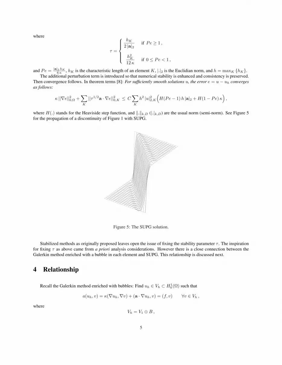
where H(.) stands for the Heaviside step function, and ‖.‖k,D (|.|k,D) are the usual norm (semi-norm). See Figure 5for the propagation of a discontinuity of Figure 1 with SUPG.

Figure 5: The SUPG solution.

Stabilized methods as originally proposed leaves open the issue of fixing the stability parameter τ . The inspirationfor fixing τ as above came from a priori analysis considerations. However there is a close connection between theGalerkin method enriched with a bubble in each element and SUPG. This relationship is discussed next.

4 Relationship

Recall the Galerkin method enriched with bubbles: Find uh ∈ Vh ⊂ H10 (Ω) such that

a(uh, v) = κ(∇uh,∇v) + (a · ∇uh, v) = (f, v) ∀v ∈ Vh ,

whereVh = V1 ⊕B ,

5

i.e. vh ∈ Vh can be written as:vh = v1 + vb ,

where v1 ∈ V1 and vb ∈ B.Since V1 ⊂ Vh and B ⊂ Vh decompose Vh in a direct sum, we can rewrite the Galerkin method as:

a(u1 + ub, v1) = (f, v1) ∀v1 ∈ V1 ,a(u1 + ub, vb) = (f, vb) ∀vb ∈ B .

If we solve for the bubble degrees-of-freedom in the second equation and substitute in the first equation ub = ub(u1, f)(a.k.a. static condensation), the resulting method is related to SUPG, in the case when V1 is the space of piecewise-linears.

Here is the argument: Let ub be spanned by a single bubble shape function on each element, then

ub =Nel∑

K=1

cKϕK , (1)

where Nel is the total elements of the partition.Then taking vb = ϕK into the second equation above at element K:

a(ub, ϕK)K = (f, ϕK)K − a(u1, ϕK)K ,

and using (1) and integrating by parts, it holds

cKa(ϕK , ϕK)K = (f − L∗u1, ϕK)K . (2)

Here L∗ denotes the adjoint operator.Now, the coefficient cK above might be written with respect to residuals. In fact, integrating by parts and using

ϕ |∂K = 0 we arrive at

a(ϕK , ϕK)K = κ||∇ϕK ||2K − (a · ∇ϕK , ϕK)K + (a · n, ϕ2K)∂K

= κ||∇ϕK ||2K .

Hence, substituting the result above into (2) we get:

cK =1

a(ϕK , ϕK)K(f − a · ∇u1, ϕK)K

=1

κ||∇ϕK ||2K(f − a · ∇u1, ϕK)K

=1

κ||∇ϕK ||2K(f − a · ∇u1) |K

∫

K

ϕK . (3)

The second step of static condensation is to compute the effect of the bubbles into the linear part of the solution,i.e., compute the second term in:

a(u1, v1) + a(ub, v1) = (f, v1) ∀v1 ∈ V1 .

Note that the weak form above is of the form: Galerkin method + Perturbation terms = 0 where the perturbation termis a(ub, v1).

6

Next, from (1), integrating by parts and using ϕ |∂K = 0 it holds:

a(ub, v1) = κ(∇ub,∇v1) + (a · ∇ub, v1)

=∑

K

cK

[κ(∇ϕK ,∇v1)K + (a · ∇ϕK , v1)K

]

=∑

K

cK

[− κ(ϕK , ∆v1)K + κ(ϕK ,

∂v1

∂n)∂K

−(ϕK ,a · ∇v1)K + (ϕK ,a · n v1)∂K

]

=∑

K

cK

[− (ϕK ,a · ∇v1)K

]

=∑

K

cK

[− (a · ∇v1) |K

∫

K

ϕK

], (4)

where we used ∆v1 = 0 in K.Combining (4) with (3), we get:

a(ub, v1) =∑

K

(a · ∇u1 − f) |Kκ||∇ϕK ||2K

(a · ∇v1) |K[∫

K

ϕK

]2

=∑

K

[∫K

ϕK

]2κ |K| ||∇ϕK ||2K

(a · ∇u1 − κ∆u1 − f,a · ∇v1)K .

This is like the perturbation term of the SUPG method with:

τ =

[∫K

ϕK

]2κ |K| ||∇ϕK ||2K

. (5)

Remarks:

• When we add any (one) bubble to linear shape functions, under the assumptions given, we can reproduce SUPG,up to the definition of τ .

• The parameter τ will not be affected if we scale the bubble basis function ϕK by a constant.

• For a cubic bubble,∫

KϕK = c h2 and ||∇ϕK ||2K = c so that τ = O(h2/κ), which is the value used in the

diffusive dominated limit only.

• ub is the approximation of fine scales, and u1 represents coarse scales. The bubbles make a correction to improvethe piecewise linear solution.

• Other bubble functions can be devised so that τ = O(h/|a|2) in the advective dominated limit.

Hereafter we examine a systematic construction of bubble functions that can deal with any limit. RFB is next.

5 Residual-free bubbles (RFB)

Consider Lu = f in Ω ,u = 0 on Γ ,

7

where L is a linear elliptic differential operator, u is the unknown scalar function and f is a given source function.The variational formulation is: Find u ∈ V such that

a(u, v) = (f, v) ∀v ∈ V .

Let us split V such thatV = V1 ⊕B ,

where we recall that V1 is the space of continuous piecewise linear (or bilinear) space. Now, the space B is the rest (torecover V ).

Then, it is possible to solve the variational formulation exactly, i.e.,

u = u1 + ub ,

where u1 ∈ V1 and ub ∈ B.The variational formulation can be rewritten as:

a(u1 + ub, v1) = (f, v1) ∀v1 ∈ V1 ,a(u1 + ub, vb) = (f, vb) ∀vb ∈ B .

(6)

If, instead, we approximate the functions in B to have zero value on the boundary of each element, then

u ≈ uh = u1 + ub ,

and the second equation in (6) applies element by element, i.e.,

a(u1 + ub, vb)K = (f, vb)K ∀vb ∈ B .

This implies the PDE locally, i.e.,Lub = −(Lu1 − f) in K ,

ub = 0 on ∂K .

Residual-free bubbles, ub, are the functions satisfying these equations strongly. In one-dimensional problems withcontinuous solution the approximation is exact (see Figure 6), i.e.,

u = uh = u1 + ub .

u

u1

ub

Figure 6: One dimensional residual-free bubbles.

8

For the advective-diffusive equation:L := −κ∆ + a · ∇ ,

thus, the RFB equation is (assuming u1 is spanned by linears):−κ∆ub + a · ∇ub = −(a · ∇u1 − f) in K ,

ub = 0 on ∂K .(7)

Note that under the assumptions of piecewise constant a and f , the solution to this PDE is spanned by a singlebubble basis function:

ub |K = cKϕK .

In addition, note that ϕK is a particular case of the bubble function employed in the argument of Section 4. Withoutany loss of generality, ϕK solves:

−κ∆ϕK + a · ∇ϕK = 1 in K ,ϕK = 0 on ∂K .

(8)

Therefore the Galerkin method enriched with RFB in this case is equivalent to the SUPG method, as described inSection 4, with a τ that will be determined by the explicit solution of (8).

Note that if we multiply the differential equation by ϕK and integrate over the element, then, by integration-by-parts:

∫

K

ϕK = κ(∇ϕK ,∇ϕK)K + (a · ∇ϕK , ϕK )K

= κ||∇ϕK ||2K − (a · ∇ϕK , ϕK )K + (a · n, ϕ2K )∂K

= κ||∇ϕK ||2K . (9)

Thus,

κ||∇ϕK ||2K =∫

K

ϕK . (10)

Substituting it in the expression for τ (5):

τ =

[∫K

ϕK

]2κ |K| ||∇ϕK ||2K

=

∫K

ϕK

|K| .

Thus, all we need is the integral of the residual-free bubble basis function ϕK .To solve (8) in general is hard so we first consider κ → 0 and we solve the limit problem:

a · ∇ϕK = 1 in K ,

ϕK = 0 on ∂K− ,(11)

where ∂K− stands for the inflow boundary in an element (see Figure 7):

∂K− = x ∈ ∂K : a · n(x) ≤ 0 .

9

a

inflow boundary K

Figure 7: Element inflow boundary.

The solution to the limit problem is the pyramid with height ha/|a|2, where ha is the longest segment parallel toa contained in K (see Figure 8).

Kha

a

K

a ha

Figure 8: Advective-diffusive RFB basis function ϕK .

Then, ∫

K

ϕK =13

ha

|a|2 |K| ,

and

τ =

∫K

ϕK

|K| =13

ha

|a|2 .

Note the similarity to τ for SUPG in the advective dominated limit:

τ =12

h

|a|2 .

An error analysis for RFB can be found in [3]. As a way to avoid limit cases, we present next a more involved andgeneral alternative to compute ϕK .

6 Two-level FEM

We recall that the general RFB problem is given byLub = −(Lu1 − f) in K ,

ub = 0 on ∂K .

10

We need to devise a strategy to solve this problem in general. First instead of solving this, we compute:Lϕi = −Lψi in K ,

ϕi = 0 onK ,

where the ψi’s are the local basis functions for u1 andLϕf = f in K ,

ϕf = 0 on K .

Thus, ifu1 =

∑

i

ci ψi ,

thenub =

∑

i

ci ϕi + ϕf .

Substituting the above characterization in the first equation in (6), we get the matrix formulation∑

i

ci [a(ψi, ψj) + a(ϕi, ψj)] = (f, ψj)− a(ϕf , ψj). (12)

The effective strategy to compute problem (12) is as follows: At the pre-processing stage of a finite element code,consider approximating the differential equations for the bubble shape functions ϕi’s and ϕf by another finite elementmethod. To this end, we consider a submesh (a mesh defined for each element, see Figure 10) where we will solve thebubble differential equations with the Galerkin-least squares method (GLS), for example.

Thus for, i = 1, .., nen,

a · ∇ϕi − κ4ϕi = −a · ∇ψi in K ,

ϕi = 0 on ∂K ,

where nen denotes the total of nodes, the unknown bubble basis function ϕi can be approximated by

ϕh∗i =

∑

l

c(i)l ψ∗l ,

where K∗ is an arbitrary element in the submesh with diameter h∗ and ψ∗l is the piecewise linear basis function in thesubmesh, see Figure 9.

KSubmesh

Mesh

Figure 9: Two-level mesh.

11

K -

a

Figure 10: Submesh refines on outflow boundaries.

We then formulate the GLS method in matrix formulation as: for each i (from 1 to nen), find c(i)l , l = 1, 2, .., N∗

such that

∑

l

c(i)l [(a · ∇ψ∗l , ψ∗m) + (κ∇ψ∗l ,∇ψ∗m) + (a · ∇ψ∗l , τ a · ∇ψ∗m)] = (−a · ∇ψi,K , ψ∗m + τ a · ∇ψ∗m) ,

for m = 1, 2, .., N∗. Here N∗ is the total nodes in K.We use the stability parameter τ given as:

τ(x, P eK(x)) =hK

2|a|2 ξ(PeK(x)) ,

PeK(x) =|a(x)|2hK

6κ,

ξ(PeK(x)) =

PeK(x), if 0 ≤ PeK(x) < 1 ,1, if PeK(x) ≥ 1 .

Once the constants c(i)l ’s are found, we get the approximate residual basis function ϕh∗

i . Figures 11-12 illustrateRFB shape functions changing the advection field orientation.

12

00.02

0.04

0

0.050

0.5

1

X−axis

φ1

Y−axis

00.02

0.04

0

0.05−1

−0.5

0

X−axis

φ3

Y−axis

00.02

0.04

0

0.05−0.5

0

0.5

X−axis

φ2

Y−axis

00.02

0.04

0

0.05−0.5

0

0.5

X−axis

φ4

Y−axis

Figure 11: RFB shape functions (45 degree problem).

00.02

0.04

0

0.050

0.5

1

X−axis

φ1

Y−axis

00.02

0.04

0

0.05−1

−0.5

0

X−axis

φ3

Y−axis

00.02

0.04

0

0.05−0.5

0

0.5

X−axis

φ2

Y−axis

00.02

0.04

0

0.05−0.5

0

0.5

X−axis

φ4

Y−axis

Figure 12: RFB shape functions (60 degree problem).

Next, these approximations are then assembled to the global problem (12) in place of the exact residual-free bubblefunction ϕi. The global problem may now be solved for the piecewise-linear (bilinear) part of the solution. See Figures13-17 for numerical results using a two-level FEM approach.

13

45

a

u = 1 u = 0

u = 0u = 1

u = 0y

x10

1

Figure 13: Propagation of a discontinuity

0

0.5

1

0 0.2 0.4 0.6 0.8 1

0

0.5

1

1.5

X−axis

GLS

Y−axis

0

0.5

1

0 0.2 0.4 0.6 0.8 1

0

0.5

1

1.5

X−axis

TLFEM

Y−axis

Figure 14: GLS versus TLFEM (45 degree problem)

0

0.5

1

0 0.2 0.4 0.6 0.8 1

0

0.5

1

1.5

X−axis

GLS

Y−axis

0

0.5

1

0 0.2 0.4 0.6 0.8 1

0

0.5

1

1.5

X−axis

TLFEM

Y−axis

Figure 15: GLS versus TLFEM (60 degree problem).

14

y

x

u=1

u=0

u=2yu=1

0.5

10

Velocity

a

a

1

2

=

=

2y

0

:

Figure 16: Thermal boundary layer problem (κ = 10−6).

0

0.5

1 0

0.2

0.40

0.5

1

1.5

Y−axis

GLS

X−axis

0

0.5

1 0

0.2

0.40

0.5

1

1.5

Y−axis

TLFEM

X−axis

Figure 17: GLS versus TLFEM (thermal boundary layer problem).

7 The Discontinuous Enrichment Method (DEM)

In this case enrichment functions are not required to satisfy a zero boundary condition. They are discontinuousand continuity are enforced weakly via Lagrange multipliers. Enrichment functions are spanned by solutions of:

Lue = 0 inK , (13)

and we solve for (u1, ue, λ):

a(u1, v1) + a(ue, v1)− < λ, v1 > = (f, v1) ,

a(u1, ve) + a(ue, ve)− < λ, ve > = (f, ve) ,

− < u1 + ue, µ > = − < g, µ > ,

where λ is the Lagrange multiplier, g is a target given function, and < ., . > is the duality product over edges. Thismethod has been applied to the Helmholtz and advection-diffusion equations (see [6, 17]).

15

8 The Petrov-Galerkin Enrichment Method (PGEM)

Zero boundary conditions on element edges (or faces in 3D) characterize the RFB approach and enable staticcondensation procedure. Petrov-Galerkin enriched method (PGEM) main idea keeps such desirable local featureas it incorporates more involving boundary conditions. This is accomplished by selecting residual-free bubbles asenrichment of test functions only. As a result, a bubble equation still holds for each element and the trial enrichmentcan be condensed as a function of the piecewise component of the solution and the data.

The way as the missed boundary condition is set is the key-point. Such choice gives rise to distinctive methodsonce the expression of the multiscale component of the solution is available and substituted into the equation tested bythe piecewise polynomial component. Thereby, the method that arises is of stabilized type with an additional stability,which may differ from canonical manners using least-squares or adjoint operators, without compromising consistency.

We illustrate the PGEM by looking at it in reactive-diffusive problems (see [11, 10, 1]). Let us start by recallingthe model: Find u such that

σu − κ4u = f in Ω , (14)u = 0 on ∂Ω ,

where σ, κ ∈ R+ denote the reactive and diffusive constants, respectively, and f is a given data.The usual variational formulation for this problem is given by: Find u ∈ H1

0 (Ω) such that:

a(u, v) = (f, v) ∀ v ∈ H10 (Ω) , (15)

where

a(u, v) := σ(u, v) + κ(∇u,∇v) . (16)

We take the trial enrichment to be in the whole space H10 (Ω) and the test enrichment to be in H1

0 (Th) :=⊕∑

K H10 (K). These are enrichment to piecewise linear u1 and v1. The PGEM becomes: Find u1 + ue such

thata(u1 + ue, v1 + vb) = (f, v1 + vb) ∀ v1 + vb ∈ Vh ⊕H1

0 (Th). (17)

If we take v1 = 0 we have a bubble equation in each element as follows:

Lue = −Lu1 + f (18)= −σu1 + f, (19)

where we used the linearity of u1 in K.For this particular model, the enrichment solves an equation governed by an operator projected along the internal

boundary elements, namely,

σue − κ∂ssue = f − σu1 on ∂K, and ue = 0 at the nodes , (20)

and ue = 0 on ∂Ω.This choice makes the edge residual to be defined with respect to the residual of Lagrange equations restricted to

the edges. As a consequence, well-posedness and global boundary conditions are clearly preserved as it is the strongcontinuity of u1 + ue.

Next, combining (18) and (20) we can represent ue |K by

ue = MK(f − σu1). (21)

This formal representation is then replaced in (17) to obtain a stabilized alike method. Note that (21) needs to becomputed in details, and we do this by using basis functions for u1 in the right-hand-sides of equations (18) and (20).In Figures 18 we depict the basis functions spanning u1 + ue with κ ranging from 10−3 to 1.

16

Figure 18: Basis functions with κ = 1 (top left), κ = 10−1 (top right) and κ = 10−3 (bottom).

Let us consider f = 1/2 defined on the unit square, and subject to the boundary conditions described in Figure 19.We use the unstructured mesh shown in Figure 20.

For a fixed σ = 1 and small κ, boundary layers appear close to the domain boundary. Figure 21 shows thesolutions of the Galerkin and the PGEM, for κ = 10−6. As predicted, the present method perform better than theGalerkin method.

u = 0

u = 0x

y

1.0

u = 1

u = 1

0.0

1.0

Figure 19: Domain.

17

MESH

Figure 20: The unstructured mesh.

GALERKIN METHOD MULTISCALE METHOD

Figure 21: Comparison between Galerkin and the PGEM with κ = 10−6.

9 Concluding RemarksThe decomposition into a piecewise linear part and a local enrichment part enables numerical multiscale methods toproduce approximations that are related to stabilized methods. These approximations are of a multiscale type, wherethe local enrichment part is an approximation of fine scales. The effect of the local enrichment part on the piecewiselinear part of the solution can be viewed as a stabilizing effect of the coarse scales. Numerical multiscale methodsprovide a framework that is computable in general and we presented various strategies to attest its applicability.

18

10 AcknowledgmentsDuring the course of this work L.P. Franca was a Visiting Professor at the Federal University of Rio de Janeiro. Theauthors wish to thank the support of CNPq and Petrobras.

References[1] R. ARAYA, G. R. BARRENECHEA, L. P. FRANCA, AND F. VALENTIN, Stabilization arising from PGEM: A

review and further developments., Appl. Num. Math., 59 (2009), pp. 2065–2081.

[2] F. BREZZI, M. BRISTEAU, L. P. FRANCA, M. MALLET, AND G. ROGÉ, A relationship between stabilizedfinite element methods and the Galerkin method with bubble functions, Comput. Methods Appl. Mech. Engrg.,96 (1992), pp. 117–129.

[3] F. BREZZI, T. J. R. HUGHES, L. MARINI, A. RUSSO, AND E. SÜLI, A priori error analysis of residual-freebubbles for advection-diffusion problems, SIAM J. Numer. Anal., 36 (1999), pp. 1933–1948.

[4] F. BREZZI AND A. RUSSO, Choosing bubbles for advection-diffusion problems, Math. Models Meth. Appl. Sci.,4 (1994), pp. 571–587.

[5] A. N. BROOKS AND T. J. R. HUGHES, Streamline upwind/Petrov-Galerkin formulations for convection dom-inated flows with particular emphasis on the incompressible Navier-Stokes equations, Comput. Methods Appl.Mech. Engrg., 32 (1982), pp. 199–259.

[6] C. FARHAT, I. HARARI, AND L. P. FRANCA, The discontinuous enrichment method, Comput. Methods Appl.Mech. Engrg., 190 (2001), pp. 6455–6479.

[7] L. P. FRANCA AND S. FREY, Stabilized finite element methods: II. The incompressible Navier-Stokes equations,Comput. Methods Appl. Mech. Engrg., 99 (1992), pp. 209–233.

[8] L. P. FRANCA, S. FREY, AND T. J. R. HUGHES, Stabilized finite element methods: I. Application to theadvective-diffusive model, Comput. Methods Appl. Mech. Engrg., 95 (1992), pp. 253–276.

[9] L. P. FRANCA AND A. MACEDO, A two level finite element method and its application to the Helmholtz equation,Int. J. Num. Meth. Engrg., 43 (1998), pp. 23–32.

[10] L. P. FRANCA, A. L. MADUREIRA, L. TOBISKA, AND F. VALENTIN, Convergence analysis of a multiscalefinite element method for singularly perturbed problems., Multiscale Model. Sim.: A SIAM Inter. J., 4 (2005),pp. 839–866.

[11] L. P. FRANCA, A. L. MADUREIRA, AND F. VALENTIN, Towards multiscale functions: Enriching finite elementspaces with local but not bubble-like functions., Comput. Methods Appl. Mech. Engrg., 194 (2005), pp. 3006–3021.

[12] L. P. FRANCA AND A. NESLITURK, On a two-level finite element method for the incompressible Navier-Stokesequations, Int. J. Num. Meth. Eng., 52 (2001), p. 433.

[13] L. P. FRANCA, A. NESLITURK, AND M. STYNES, On the stability of residual-free bubbles for convection-diffusion problems and their approximation by a two-level finite element method, Comput. Methods Appl. Mech.Engrg., 166 (1998), pp. 35–49.

[14] L. P. FRANCA AND A. RUSSO, Deriving upwinding, mass lumping and selective reduced integration by residual-free bubbles, Appl. Math. Letters, 9 (1996), pp. 83–88.

19

[15] T. J. R. HUGHES, Multiscale phenomena: Green’s functions, the Dirichlet-to-Neumann formulation, subgridscale models, bubbles and the origin of stabilized methods, Comput. Methods Appl. Mech. Engrg., 127 (1995),pp. 387–401.

[16] T. J. R. HUGHES, L. P. FRANCA, AND M. BALESTRA, A new finite element formulation for compuationalfluid dynamics: V. Circumventing the Babuska-Brezzi condition: a stable Petrov-Galerkin formulation of theStokes problem accommodating equal-order interpolations, Comput. Methods Appl. Mech. Engrg., 59 (1986),pp. 85–99.

[17] I. KALASHNIKOVA, C. FARHAT, AND R. TEZAUR, A discontinuous enrichment method for the finite element so-lution of high Peclet advection-diffusion problems, Finite Elements in Analysis and Design, 45 (2009), pp. 238–250.

[18] A. MASUD AND R. KHURRAM, A multiscale finite element method for the incompressible Navier-Stokes equa-tions, Comput. Methods Appl. Mech. Engrg., 195 (2006), pp. 1750–1777.

20