Three-Dimensional Mesoscale Dipole Frontal Collisions

SARA DUBOSQ* AND ÁLVARO VIÚDEZ

Institut de Ciències del Mar, CSIC, Barcelona, Spain

(Manuscript received 6 July 2006, in final form 3 November 2006)

ABSTRACT

Frontal collisions of mesoscale baroclinic dipoles are numerically investigated using a three-dimensional,Boussinesq, and f-plane numerical model that explicitly conserves potential vorticity on isopycnals. Theinitial conditions, obtained using the potential vorticity initialization approach, consist of twin baroclinicdipoles, balanced (void of waves) and static and inertially stable, moving in opposite directions. The dipolesmay collide in a close-to-axial way (cyclone–anticyclone collisions) or nonaxially (cyclone–cyclone or an-ticyclone–anticyclone collisions). The results show that the interacting vortices may bounce back andinterchange partners, may merge reaching a tripole state, or may squeeze between the outer vortices. Theformation of a stable tripole from two colliding dipoles is possible but is dependent on diffusion effects. Itis found that the nonaxial dipole collisions can be characterized by the interchange between the domain-averaged potential and kinetic energy. Dipole collisions in two-dimensional flow display also a variety ofvortex interactions, qualitatively similar to the three-dimensional cases.

1. Introduction

Mesoscale vortical structures are frequent phenom-ena in the oceans and atmosphere, and the vortex di-pole, also called vortex pair, vortex couple, double-vortex, or mushroomlike vortex, is one of the simplestamong these mesoscale structures (Carton 2001). Innonrotating fluids, for example, dipoles are spontane-ously generated in Von Kármán wakes in two-di-mensional turbulence (Couder and Basdevant 1986). Adipolar solution in nonrotating two-dimensional fluids,different from the Lamb dipole, was recently found byJuul Rasmussen et al. (1996).

Vortex dipoles have been observed in many places inthe ocean (e.g., Fedorov and Ginzburg 1986; Munk etal. 1987), including the Alaska Coastal Current (Ahlnäset al. 1987), along the Vancouver Island coast (Ikeda etal. 1984), along the California coast (Sheres andKenyon 1989; Simpson and Lynn 1990), south of Mada-gascar (de Ruijter et al. 2004), in Tartar Strait (Ginz-

burg and Fedorov 1984), in the Norwegian Coastal Cur-rent (Johannessen et al. 1989), and in the OyashioFront (east of Japan; Vastano and Bernstein 1984).

Laboratory experiments in rotating tanks show thatbarotropic dipoles can be generated from an impulsivejet (Kloosterziel et al.1993), become important trans-porters of fluid (Eames and Flór 1998), and finally de-cay—for example, because of bottom friction effects(Sansón et al. 2001). Theoretically, Stern (1975) derivedan exact dipolar solution, for nondivergent barotropicflow on the � plane, called the modon (Flierl et al. 1983;McWilliams 1983; Berson and Kizner 2002, and refer-ences therein). Numerically, the generation of oceanicdipoles was investigated using a two-layer, f plane, shal-low-water model by Mied et al. (1991).

Since the dipole is a coherent vortical structure witha propagation speed, it may approach a coast or ob-stacle and rebound (Carnevale et al. 1997; Danaila2004), interact with a sloping boundary (Kloosterziel etal. 1993), or interact with a jet (Vandermeirsh et al.2002). The dipoles may also generate or interact withinertia–gravity waves (Afanasyev 2003; Godoy-Dianaet al. 2006). Furthermore, interactions between dipoles,or collisions, are also possible. These interactions mayoccur in a number of ways, namely, frontal or head-onaxial collisions, head-back (dipole overtaking or merg-ing) axial collisions, oblique collisions, or frontal non-axial collisions (Voropayev and Afanasyev 1994, chap-

* Additional affiliation: École Nationale Supérieure de Tech-niques Avancées, Paris, France.

Corresponding author address: Sara Dubosq, Clayrac, 81630Salvagnac, France.E-mail: sara.dubosq@free.fr

SEPTEMBER 2007 D U B O S Q A N D V I Ú D E Z 2331

DOI: 10.1175/JPO3105.1

© 2007 American Meteorological Society

JPO3105

ter 4). Laboratory experiments, in nonrotating plat-forms, have reproduced axial head-on dipole collisions,and subsequent vortex partner interchange (van Heijstand Flór 1989), as well as oblique dipole collisions(Voropayev and Afanasyev 1992). Two-dimensionalnumerical simulations, in nonrotating fluids, of obliquedipole collisions were carried out by Couder and Bas-devant (1986) in the context of two-dimensional turbu-lence. Head-on and overtaking dipole collisions ofbarotropic equivalent modons on the � plane were nu-merically investigated by McWilliams and Zabusky(1982). Laboratory experiments in rotating fluids on a �plane, confirmed by point-vortex numerical simula-tions, have shown that nonaxial dipole collisions lead toa large mass exchange between the dipoles or the am-bient fluid (Velasco Fuentes and van Heijst 1995).

Here, we take a step forward in our understanding ofdipole interactions by numerically investigating non-axial frontal collisions of mesoscale baroclinic dipoles.Since the vortices are easily characterized by their con-served potential vorticity (PV), we use, as a primarymodel, a three-dimensional numerical algorithm thatexplicitly conserves PV on isopycnals (described in sec-tion 2). The initial conditions, obtained using the PVinitialization approach, consist of twin baroclinic di-poles moving in opposite directions (section 3a). Thetranslating dipoles are balanced (void of waves) andremain always static and inertially stable. We describesix different classes of possible collisions, which dependon the initial distance between the dipoles axes of mo-tion. These cases include the axial cyclone–anticyclonecollision (section 3b) and the nonaxial anticyclone–anticyclone (section 3c) and cyclone–cyclone (section3d) collisions. We show that, besides the familiar close-to-axial collision, there is a rich variety of vortex inter-actions during the dipole collisions, including vortexmerging and splitting, vortex bouncing, vortex squeez-ing, and tripole formation. These processes involve in-terchange between the domain averaged kinetic andpotential energy. Dipole collisions in two-dimensionalflow are also numerically investigated (section 3e), re-sulting also in a variety of vortex interactions, qualita-tively similar to the three-dimensional cases.

2. Numerical model and parameters

The time evolution of the three-dimensional (baro-clinic) dipoles is simulated using a triply periodic, vol-ume-preserving, nonhydrostatic numerical model withthe Boussinesq and f-plane approximations (Dritscheland Viúdez 2003) initialized using the PV initializationapproach (Viúdez and Dritschel 2003). The vertical dis-placement D of isopycnals with respect to the reference

density configuration is D(x, t) � z � d(x, t), whered(x, t) � (�(x, t) � �0)/�z is the depth, or vertical loca-tion, that an isopycnal located at x at time t has in thereference density configuration defined by �0 � �zz,where � is the density, and �0 � 0 and �z � 0 are givenconstants. Static instability occurs when Dz � �D /�z �1. The Rossby number R � /f, and the Froude numberF � h /N , where h and are the horizontal and ver-tical components of the relative vorticity �, respec-tively, f is the constant Coriolis frequency, and N is thetotal Brunt–Väisälä frequency. We simulate here baro-clinic dipoles in the regime of static (Dz � 1) and iner-tial stability (|R |� 1) so that the flow remains largely inhydrostatic balance.

The dimensionless PV anomaly � � � � 1, where� � (� /f � k) · �d is the dimensionless total PV, isrepresented by contours lying on isopycnals, and PVmaterial conservation (d�/dt 0) is made explicit byPV contour advection. The state variables are the com-ponents of the vector potential � (�, �, � ), whichprovide the velocity u (u, �, w) �f � � � and thevertical displacement of isopycnals D ��2� · �,where � � c�1 � f /N is the ratio of f to the meanBrunt–Väisälä frequency N. Since � is triply periodic,u and D are triply periodic as well, while obviously d (or�) is not. This numerical model (referred to as the AB�model) integrates the horizontal components of thedimensionless ageostrophic vorticity Ah � (A , B) ��h/f � c2�hD (appendix A). The horizontal potentials�h (�, �) are obtained every time step by inverting�2�h Ah, while the vertical potential � is obtained byinverting the definition of �(�, �, � ).

The total energy ET � EK � EP, where EK � u2 ��2 � w2 and EP � N2D 2 are the kinetic and potentialenergy, respectively. The domain-averaged total energy�ET� is conserved (appendix B), where

�E��t� �1

nxnynz�i 1

nx

�j 1

ny

�k 1

nz

E�xi, yj, zk, t� �1�

is the domain average of any field E , and nx, ny, and nz

are the dimensions of the numerical grid.We use an nx � ny � nz 1283 grid, with nl 128

isopycnal layers, in a domain of vertical extent Lz 2�(which defines the unit of length) and horizontal ex-tents Lx Ly cLz, with c 100. We take the (mean)buoyancy period (Tbp � 2�/N) as the unit of time bysetting N � 2�. One inertial period (Tip � 2�/f ) equals100Tbp. The time step �t 0.05, and initialization timetI 5Tip. The initialization time is the minimum timerequired for the fluid to reach its initial perturbed statewith minimal generation of inertia–gravity waves.

To avoid the generation of grid-size noise, a bi-

2332 J O U R N A L O F P H Y S I C A L O C E A N O G R A P H Y VOLUME 37

harmonic hyperdiffusion term � �(�4qA , �4

qB), where�q� � (�� /�x, ��/�y, ���/�z) is the gradient operator inthe vertically (quasigeostrophic) stretched space, isadded to the equations for the rate of change of Ah. Thehyperviscosity coefficient � is chosen by specifying thedamping rate (e-folding, ef) of the largest wavenumberin spectral space per inertial period, which was set con-stant to 10.

As a secondary numerical model we use the full pseu-dospectral version of the hybrid AB� algorithm (appen-dix A). This model, referred to as the ABC model, usesthe same grid-based procedures as the AB� model ex-cept that it does not use any of the procedures involvingthe PV contours. The prognostic variables are A � (A,B, C)� �/f� c2�D. Hence, there is no inversion of PV,but only a Poisson equation for all three components ofthe vector potential, �2� A, which is inverted spec-trally every time step. All the parameter settings are thesame except for the hyperviscous damping rate, whichwas significantly increased to maintain numerical sta-bility.

3. Numerical results

a. Initial dipole configuration

The initial dipole consists of two baroclinic vortices,each one defined by a three-dimensional ellipsoidal dis-tribution of PV anomaly �, constant on ellipsoidal sur-faces, which varies linearly with the ellipsoidal volume,with� 0 on the outermost surface, and�min �0.75and �max 0.75 at the center of the cyclone and anti-cyclone, respectively (Fig. 1a). The PV distribution isdiscretized by placing a number of PV contours withineach isopycnal surface crossing through the vortex. Themiddle isopycnal surface (il 65) has the maximumnumber of contours (nc 10). The initial PV contoursare ellipses with a ratio of major (ax) to minor (ay)

semiaxes lengths ax/ay 1.5. The largest ellipse, locatedon the middle isopycnal surface, has ax 0.6c and ay 0.4c. The vortex ellipsoidal shape is initially prescribedonly to facilitate the transition toward an equilibriumshape, largely independent on the initial conditions,reached at the end of the initialization time (explainedbelow).

The vertical semiaxes are a�z 0.4 and a�z 0.27 forthe cyclone (� � 0) and the anticyclone (� � 0), re-spectively. These values were chosen so that the dipoledescribed a straight trajectory (Figs. 1b,c). This asym-metry in the vertical extent of the vortices is due to thePV anomaly being prescribed in the reference configu-ration (flat isopycnals) at the beginning of the initial-ization time (t� 0). During the initialization period(from t� 0 to 5Tip) the isopycnals stretch (in the an-ticyclone) and shrink (in the cyclone) to reach a bal-anced state so that the final adjusted state of the dipoleis not exactly antisymmetric. For the initial conditions(t 0) of the collision simulations we use the state ofthe dipole at t� 19Tip (Fig. 1c, hereinafter just re-ferred to as the initial dipole configuration). At thisstage the PV vortices have long time ago deformedfrom their initial ellipsoidal configuration. Thus, thislarge period of time (19Tip) assures that the initial PVconfiguration of the dipoles has been adjusted to asteady PV distribution.

In the initial dipole configuration the horizontal ve-locity uh in the anticyclone is somewhat larger than inthe cyclone (Fig. 2a), with the maximum horizontal ve-locity, reaching umax � max{|uh|} 0.77, located at thecenter of the dipole. The vertical velocity w (Fig. 2b) is104 times smaller than |uh|, and presents the quadrupo-lar pattern typical of mesoscale quasigeostrophic bal-anced dipoles (Pallàs-Sanz and Viúdez 2006). The iso-pycnal displacement D (D � 0 in the anticyclone; Fig.2c) and the vertical vorticity ( � 0 in the anticyclone;

FIG. 1. Potential vorticity anomaly contours (PV jumps) on the middle isopycnal (il 65) at (a) t� 0, (b) t� 10Tip, and (c) t� 19Tip. PV jump value �� � 0.075 (difference between two consecutive PV contours). Thehorizontal extent is �x �y 2�c/3. The x coordinate of the origin (x0) is (b) 0.85 and (c) 1.5 relative to (a).

SEPTEMBER 2007 D U B O S Q A N D V I Ú D E Z 2333

Fig. 2d) have similar vertical extents in both vortices.The relative vorticity changes sign on the northern andsouthern sides of the dipole with both | | and |D | in theanticyclone larger than in the cyclone. The dipole isstatic and inertially stable with Dzmax � max{Dz(x)} 0.36, R min � min{R (x)} �0.62, R max � max{R (x)} 0.41, and Fmax � max{F (x)} 0.32 at t 0.

Last, the initial PV configuration of the two-dipolefrontal collision simulations is obtained by adding, tothe dipole described above (left dipole, L in Fig. 3), ay-inverted copy of dipole L (right dipole, R in Fig. 3)separated from L by �X � �c (fixed) and �Y (vari-able). The initially prescribed y-offset �Y makes theinitial location of the dipoles change along lines L andR in Fig. 3. Specification of �Y defines, therefore, thedifferent numerical simulations described below. Sincethe two-dipole PV configuration is now different fromthe previous single dipole configuration, the numericalsimulations are initialized from t 0 to 5Tip, usingagain the PV initialization approach. The actual y-off-set between the dipoles, that is, at the end of the ini-tialization period (t 5Tip), is defined as Y � YR � YL,where the y coordinate of the L and R dipole are thegeometric centers of the pair of vortices,

YL �Y L� � Y L

�

2and YR �

Y R� � Y R

�

2, �2�

where the y coordinates Y R and Y L of every vortex aredefined as

Y R� �

���V R�

��x, tI� y dV

���V R�

��x, tI� dV

, etc., �3�

where the integration volumes V L and V

R comprisethe grid locations with |�| � 0.1. We define the dimen-sionless y-offset � as Y per unit of dipole y extent,

� �Y

4ay. �4�

After the initialization time, the dipoles explicitly con-serve PV and approach each other almost steadilyalong the axes y YL (dipole L) and y YR (dipole R).

b. P–N collision

We describe first the familiar frontal, close-to-axialdipole collision. As an example we show a case with

FIG. 3. PV contours at t 0 on isopycnal il 65 (z 0). Theinitial configuration in every case is obtained by shifting horizon-tally the left and right dipoles (comprising vortices L and R )along the L and R lines. The entire domain �x �y 2�c isshown.

FIG. 2. (a) Horizontal distribution at t 0 (t� 19Tip) and z 0 (iz 65) of the horizontal velocity uh (u, �) (onlyevery other vector is plotted). Contours of |uh| are included with contour interval � 0.1 and max{|uh|} 0.77. (b)Horizontal distribution at z �0.147 (iz 62) of vertical velocity w (� 10�5, w ∈ [�5.2, 6.4] � 10�5). South–northvertical distributions at x �0.49 (ix 55, across the dipole center) of (c) vertical displacement of isopycnals D (� 0.5 � 10�2, D ∈ [�7.7, 5.6] � 10�2), and (d) vertical vorticity (� 2.5 � 10�3, ∈ [�3.9, 2.6] � 10�2). Horizontal andvertical extents are �x �y 2c and �z 2, respectively.

2334 J O U R N A L O F P H Y S I C A L O C E A N O G R A P H Y VOLUME 37

� �0.27 (Fig. 4). The dipoles collide in such way thatthe interaction occurs between vortices of opposite PVsign; that is, we have L�–R� and L�–R� interactions.We refer to this case as a P–N collision (positive–negative PV collision). The dipole interaction occursbetween t 14Tip and 20Tip, when the dipoles inter-change vortex partners cleanly, with little PV mixingbetween vortices. After collision, the new dipoles leavethe impinging region and propagate with a straight tra-jectory, which can be approximately obtained followingthe relative extrema of � during the numerical simula-tion (Fig. 5a). Owing to the negative �, the new axis ofmotion is however not perpendicular to the original one(along constant y). In this case, the angle between oldand new dipoles trajectories (!, defined from the tra-jectory of vortex R�) is ! � �/2. An initial � 0 (per-fectly axial collision) results in new dipole trajectoriesperpendicular to the original ones (! �/2), while � �0 results in new dipole trajectories with ! � �/2 (notshown). We show later that the P–N collision is typicalfor a range of values �min � � � �max, where �0.52 ��min and �max � 0.20.

In this P–N case, the flow before, during, and afterthe collision remains always static and inertially stablewith |Dz| � 1 and |R | � 1. Extreme Rossby and Froudenumbers remain quite constant during the dipoles in-teraction (Table 1). Both umax and maximum verticalvelocity wmax � max{w} decrease and Dmax increases

slightly before the dipoles collision, and the oppositechanges happen after collision (Figs. 6 and 7a). Thus,some deceleration (acceleration) of the flow, at least inthe extreme values, occurs before (after) collision. Nu-merically, �ET� is well conserved (Fig. 8a), and there islittle interchange between �EK� and �EP� in the flow(Fig. 8b).

c. N–N collision

We describe next two different classes of dipoles col-lisions in which the dipole interaction occurs mainlybetween the anticyclonic vortices (N–N collisions).

1) CASE N–N(1)

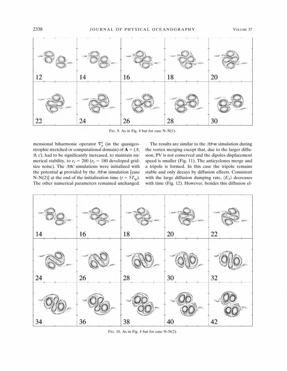
In this case � �0.52 is smaller than in the previouscase so that only the anticyclones collide (collision L�–R�; Fig. 9). The interaction between the anticyclonesresembles, in some way, an elastic collision betweensolid bodies. There is some mass transfer between theinteracting anticyclones (between t � 16–24Tip), al-though their core remain largely isolated.

The anticyclones do not merge due to the influenceof the cyclones. The gradient pressure force exerted bythe outer cyclones induces a linear momentum, in thenew anticyclone partners, opposite to the initial dipolemomentum, preventing the merging of the two anticy-clones and causing the change in direction of the newdipoles. After collision, the anticyclones bounce back

FIG. 4. Time evolution of PV contours on isopycnal il 65 (z 0) for case P–N (time in Tip, �x �y 2�c).

FIG. 5. Grid locations (ix, iy) where |� (ix, iy)| � 0.74 at z 0 (iz 65) from t 0 to the end of thenumerical simulations. Dark areas (grid points marked with symbol *) mean � � �0.74, and light areas(symbol �) mean � � 0.74, for cases (a) P–N, (b) N–N(1), and (c) N–N(2).

SEPTEMBER 2007 D U B O S Q A N D V I Ú D E Z 2335

and join the cyclone of the companion dipole, whichexperiences no trajectory curvature change (Fig. 5b).Thus, this case may be considered as a limit case of thepreviously described class P–N since here, qualitativelyspeaking, the percentage of positive–negative PV colli-sion may be taken as zero, the percentage of negative–negative PV collision as 100%, and ! 0.

As in case P–N, umax reaches a minimum (Fig. 6a),and D a maximum (Fig. 7a), during the interaction pe-riod, with Dmax larger than in case P–N. Here, how-ever, w reaches a maximum during this period (Fig. 6b);Dzmax reaches a significant maximum when the cyclonescollide (Fig. 7b). This maximum is due to the fact thatthe colliding anticyclones (which partially merge) havelarger Dz (Fig. 2c) than the cyclones (which do notmerge). In this case R max and Fmax are very similar tothose in the case P–N (Table 1). The ratio �EP�/�ET�reaches a maximum during the collision, and therefore�EK�/�ET� reaches a minimum (Fig. 8b). Thus, there isan interchange between �EK� and �EP�. This inter-change seems to be due to the deceleration of the flowand deepening of isopycnals during the collision.

The �ET� experiences, however, an increment��ET� � 0.02/2.07 � 0.01 1%, relative to its initialvalue (Fig. 8a). This nonconservative change is related

to the intrinsic numerical diffusion associated to thediscretization of the PV field (which implies contourmerging during the anticyclones partial merging). Weaddress this numerical process in the next case wherethe vortex merging is larger and, therefore, its effectson �ET� are more important.

2) CASE N–N(2)

If � is decreased by a small amount relative to theprevious case N–N(1), setting � �0.56 (i.e., a 7%decrease), the evolution of the dipoles collision is verydifferent (Fig. 10). Initially (t � 16–20Tip) the anticy-clones collide in a way similar to the case N–N(1) (Fig.9). However, here the anticyclones almost fully mergeso that the vortical structure transforms into a tripole.The tripole rotates (t 22–34Tip) with a negative (an-ticyclonic) phase speed, completing at least a rotationof 90° during about 12 inertial periods (Fig. 5c). Thetripole is unstable and eventually the anticyclone splits(t 34–36Tip), and the two-dipole system is recoveredwith an axis of motion rotated about 90° relative to theinitial axis. The rotation angle of the axis of motiondepends on �, first increasing with decreasing �, reach-ing a maximum value of about 150°, and decreasingafterwards. A stable tripole was not found.

FIG. 6. Time evolution of (a) umax and (b) wmax (�10�4) for the different cases (time in Tip).

TABLE 1. Extreme and time-averaged values of R min, R max, F max, and Dz max for the different cases. The time average ranges fromt1 5Tip to t2 {40, 40, 45, 40, 33, 35}Tip (standard deviations are included).

Case R min R max Fmax Dzmax R min R max Fmax Dzmax

P–N �0.63 0.43 0.35 0.37 �0.62 ( 0.002) 0.42 ( 0.01) 0.34 ( 0.009) 0.37 ( 0.001)N–N(1) �0.63 0.43 0.36 0.43 �0.62 ( 0.003) 0.41 ( 0.009) 0.34 ( 0.01) 0.38 ( 0.02)N–N(2) �0.65 0.43 0.36 0.47 �0.63 ( 0.01) 0.41 ( 0.01) 0.34 ( 0.01) 0.40 ( 0.03)P–P(1) �0.63 0.45 0.35 0.37 �0.62 ( 0.002) 0.42 ( 0.02) 0.34 ( 0.006) 0.37 ( 0.002)P–P(2) �0.63 0.50 0.31 0.36 �0.62 ( 0.002) 0.43 ( 0.03) 0.33 ( 0.01) 0.37 ( 0.001)P–P(3) �0.63 0.52 0.35 0.37 �0.62 ( 0.002) 0.43 ( 0.03) 0.34 ( 0.01) 0.37 ( 0.002)

2336 J O U R N A L O F P H Y S I C A L O C E A N O G R A P H Y VOLUME 37

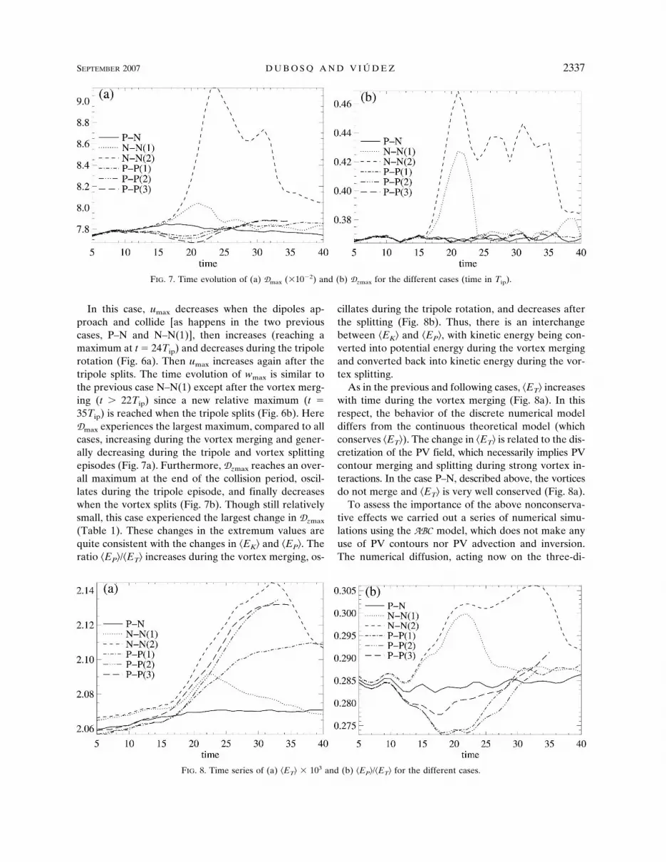
In this case, umax decreases when the dipoles ap-proach and collide [as happens in the two previouscases, P–N and N–N(1)], then increases (reaching amaximum at t 24Tip) and decreases during the tripolerotation (Fig. 6a). Then umax increases again after thetripole splits. The time evolution of wmax is similar tothe previous case N–N(1) except after the vortex merg-ing (t � 22Tip) since a new relative maximum (t 35Tip) is reached when the tripole splits (Fig. 6b). HereDmax experiences the largest maximum, compared to allcases, increasing during the vortex merging and gener-ally decreasing during the tripole and vortex splittingepisodes (Fig. 7a). Furthermore, Dzmax reaches an over-all maximum at the end of the collision period, oscil-lates during the tripole episode, and finally decreaseswhen the vortex splits (Fig. 7b). Though still relativelysmall, this case experienced the largest change in Dzmax

(Table 1). These changes in the extremum values arequite consistent with the changes in �EK� and �EP�. Theratio �EP�/�ET� increases during the vortex merging, os-

cillates during the tripole rotation, and decreases afterthe splitting (Fig. 8b). Thus, there is an interchangebetween �EK� and �EP�, with kinetic energy being con-verted into potential energy during the vortex mergingand converted back into kinetic energy during the vor-tex splitting.

As in the previous and following cases, �ET� increaseswith time during the vortex merging (Fig. 8a). In thisrespect, the behavior of the discrete numerical modeldiffers from the continuous theoretical model (whichconserves �ET�). The change in �ET� is related to the dis-cretization of the PV field, which necessarily implies PVcontour merging and splitting during strong vortex in-teractions. In the case P–N, described above, the vorticesdo not merge and �ET� is very well conserved (Fig. 8a).

To assess the importance of the above nonconserva-tive effects we carried out a series of numerical simu-lations using the ABC model, which does not make anyuse of PV contours nor PV advection and inversion.The numerical diffusion, acting now on the three-di-

FIG. 7. Time evolution of (a) Dmax (�10�2) and (b) Dzmax for the different cases (time in Tip).

FIG. 8. Time series of (a) �ET� � 103 and (b) �EP�/�ET� for the different cases.

SEPTEMBER 2007 D U B O S Q A N D V I Ú D E Z 2337

mensional biharmonic operator �4q (in the quasigeo-

strophic stretched or computational domain) of A (A ,B, C), had to be significantly increased, to maintain nu-merical stability, to ef 200 (ef 180 developed grid-size noise). The ABC simulations were initialized withthe potential � provided by the AB� simulation [caseN–N(2)] at the end of the initialization time (t 5Tip).The other numerical parameters remained unchanged.

The results are similar to the AB� simulation duringthe vortex merging except that, due to the larger diffu-sion, PV is not conserved and the dipoles displacementspeed is smaller (Fig. 11). The anticyclones merge anda tripole is formed. In this case the tripole remainsstable and only decays by diffusion effects. Consistentwith the large diffusion dumping rate, �ET� decreaseswith time (Fig. 12). However, besides this diffusion ef-

FIG. 9. As in Fig. 4 but for case N–N(1).

FIG. 10. As in Fig. 4 but for case N–N(2).

2338 J O U R N A L O F P H Y S I C A L O C E A N O G R A P H Y VOLUME 37

fect, the �EK� and �EP� behave in a way similar to theAB� simulation during the vortex merging, where �EP�/�ET� increases. Further �EK�–�EP� interchange is relatedto oscillations in the cyclones trajectories around theanticyclone. Note that the change of �ET� in the AB�simulation amounts for a change (per Tip) of � � 0.1%of its initial value, while � � �0.3% in the ABC simu-lation. Thus, the process of reaching a stable tripolefrom a two-dipole collision is related to diffusion effectstypical of an irreversible dynamics since the reverseprocess (namely a stable tripole splitting into two di-poles) is a contradiction. The formation of an unstabletripole, followed by tripole splitting, and recovery ofthe two-dipole system is more consistent with a revers-ible dynamics.

d. P–P collision

We describe next three classes of frontal dipoles col-lisions in which � � 0 so that the dipoles interactthrough the positive PV vortices.

1) CASE P–P(1)

In this case � 0.20, the cyclones collide, partiallymerge, but finally split and, in a way similar to caseN–N(1), bounce back interchanging the anticyclonicpartner (Fig. 13). Though there is considerable vortexmerging, the PV core of the cyclones remains isolated(Fig. 14a). The PV filamentation is, however, largerthan in the case N–N(1), and the cyclones after theinteraction become weaker than the anticyclones, sothat the resulting dipoles have negative trajectory cur-vature.

Similar to the previous cases, umax decreases duringthe vortex merging (t 15–19Tip) and increases duringthe vortex splitting (t 23–31Tip) (Fig. 6a). Contrary tothe N–N cases, Dmax decreases during the vortex merg-ing and increases during the vortex splitting (Fig. 7a).These changes of D are probably related to the largedeformation of the cyclones, in comparison to the de-formation of the anticyclones in the cases N–N, dur-ing the vortex interaction (cf. Fig. 13 with Figs. 9 and

FIG. 12. Time series of E � �E � � �E � for E ET � 104, EK � 0.5 � 104, EP � 104,EK/ET� 102, and EP/ET� 102. The time average ( ) ranges over t 5–60Tip, with �ET� 18.5� 10�4, �EK� 13.3 � 10�4, �EP� 5.24 � 10�4, �EK/ET� 71.7 � 10�2, and�EP/ET� 28.3 � 10�2.

FIG. 11. Time evolution from t 5Tip to t 75Tip of �(x, y) at z 0 for the ABC simulation of case N–N(2). Discontinuouscontours mean � � 0, contour interval � 0.08, and x, y ∈ [�2.4, 2.4].

SEPTEMBER 2007 D U B O S Q A N D V I Ú D E Z 2339

10). Consequently, �EP�/�ET� decreases during the cy-clone merging and increases during the cyclone splitting(Fig. 8b).

2) CASE P–P(2)

In this and the following case, the interchange of thevortex partners is not so clear as in the previous case.Here � 0.24; that is, 8% larger than in P–P(1), apercentage similar to that between cases N–N(1) andN–N(2). The cyclones collide and fully merge forming atransitory tripole (Fig. 15). This process is, thus, similarto N–N(2) except that here the vortex merging occursbetween the cyclones and the tripole splits faster intotwo dipoles with little change in the anticyclones tra-jectories (Fig. 14b). These differences are probably dueto the amount of PV (i.e., the volume integration of �)in the cyclone being smaller than in the anticyclones(Figs. 2c,d).

As is characteristic of the P–P collision, the deforma-tion of the cyclone is larger than the deformation of theanticyclones of the N–N collisions. This implies thatDmax and �EP�/�ET� decrease during the cyclone merg-ing (t 15–21Tip) and increase during the cyclonesplitting (Figs. 7a and 8b).

3) CASE P–P(3)

For the last case, we slightly increase � 0.36, that is,a 26% increase relative to P–P(1). In this case the cy-

clones collide but do not fully merge (Fig. 16). Thus,there is no interchange of vortex partners as happens incase P–P(1) (Fig. 13). This case is very similar to theprevious P–P(2) except that here the cyclonic cores re-main mostly isolated, so a tripole episode is not com-pletely reached (cf. Figs. 14b,c). This case is the onlyone in which umax increases during the cyclones im-pingement (Fig. 6a). This increase of umax is probablyrelated to the fact that the interacting cyclones have tosqueeze between the anticyclones, which, having largeramount of PV anomaly, remain more stable and static.

e. Two-dimensional dipole collisions

Numerical simulations with the �2D model, the two-dimensional (2D) version of the AB� model (appendixA), have been also carried out for comparison with the3D results. The process to obtain the initial conditionsfor the 2D dipole was similar to the one in the 3Dsimulations, using a 2D dipole with the same initial PVvalue (�max ��min 0.75) and geometry, and inthe 2D case selecting the adjusted state at t � 15Tip.Though a case-to-case comparison is not strictly pos-sible since a 2D vortex is an entity different from abaroclinic 3D vortex, and the PV criterion is not theunique one to relate both cases, we found that, depend-ing on the y offset, the dipoles may interchange part-ners or squeeze between the outer vortices as in the 3Dcase. A transient 2D tripole state, as long-lasting as in

FIG. 14. As in Fig. 5 but for cases (a) P–P(1), (b) P–P(2), and (c) P–P(3).

FIG. 13. As in Fig. 4 but for case P–P(1).

2340 J O U R N A L O F P H Y S I C A L O C E A N O G R A P H Y VOLUME 37

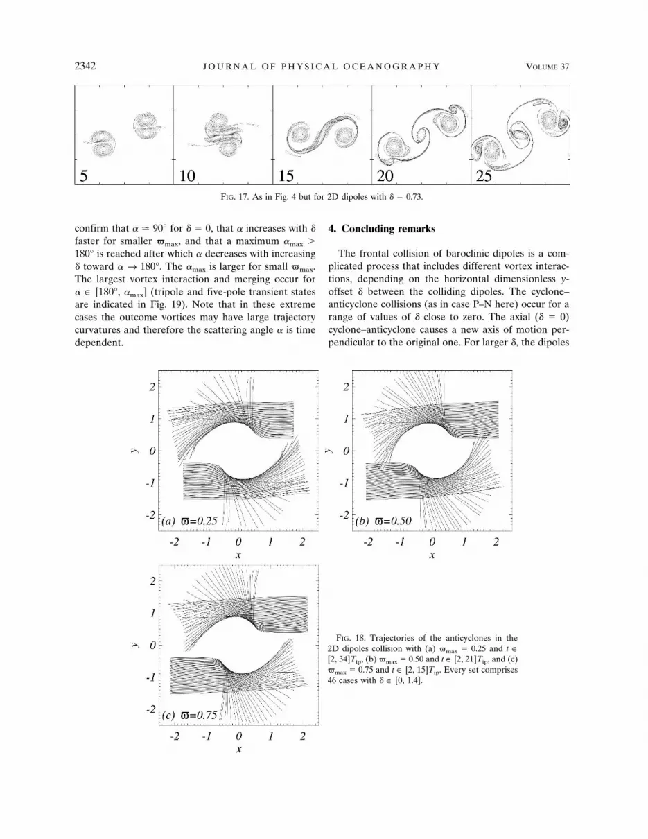
the 3D case, was not found (with �max 0.75). This isprobably due to the larger propagation speed of thedipoles relative to the 3D ones with the same �.However, it was observed as a new temporary state, afive-pole structure (Fig. 17). During the dipole collisionthe inner vortices (the cyclones in this case) merge anda tripole is temporarily formed. The anticyclones arehowever strong enough to tear apart the cyclone, whichsplits in three small cyclones, forming two dipoles witha central cyclone. The dipoles are asymmetric and havea large trajectory curvature.

Longer-lasting temporary tripole states are also pos-sible with 2D dipoles of vortices with smaller �. Thetrajectories of the outer vortices, which are easier tofollow since they do not merge, are displayed in Fig. 18for dipoles with �max 0.25, 0.50, and 0.75, respec-

tively. In the three cases the dipoles behave qualita-tively in a similar way. For small � the vortices exchangepartners and change 90° from their trajectory. As �increases, so does the scattering angle !, up to a maxi-mum value !max after which it diminishes since the di-poles no longer interact. Note that ! increases fasterwith � for small �max (there is a smaller number oftrajectories pointing northward and southward in Fig.18a than in Fig. 18c), which is due to the fact that thedipoles with small�max have slower speed and interact,therefore, during longer times than the dipoles withlarge �max.

The scattering angle ! as a function of � is shown inFig. 19 for the three PV cases. The scattering angle iscomputed by fitting the first and last five points of everytrajectory in Fig. 18 to a straight segment. The results

FIG. 16. As in Fig. 4 but for case P–P(3).

FIG. 15. As in Fig. 4 but for case P–P(2).

SEPTEMBER 2007 D U B O S Q A N D V I Ú D E Z 2341

confirm that ! � 90° for � 0, that ! increases with �faster for smaller �max, and that a maximum !max �180° is reached after which ! decreases with increasing� toward ! → 180°. The !max is larger for small �max.The largest vortex interaction and merging occur for! ∈ [180°, !max] (tripole and five-pole transient statesare indicated in Fig. 19). Note that in these extremecases the outcome vortices may have large trajectorycurvatures and therefore the scattering angle ! is timedependent.

4. Concluding remarks

The frontal collision of baroclinic dipoles is a com-plicated process that includes different vortex interac-tions, depending on the horizontal dimensionless y-offset � between the colliding dipoles. The cyclone–anticyclone collisions (as in case P–N here) occur for arange of values of � close to zero. The axial (� 0)cyclone–anticyclone causes a new axis of motion per-pendicular to the original one. For larger �, the dipoles

FIG. 18. Trajectories of the anticyclones in the2D dipoles collision with (a) �max 0.25 and t ∈[2, 34]Tip, (b) �max 0.50 and t ∈ [2, 21]Tip, and (c)�max 0.75 and t ∈ [2, 15]Tip. Every set comprises46 cases with � ∈ [0, 1.4].

FIG. 17. As in Fig. 4 but for 2D dipoles with � 0.73.

2342 J O U R N A L O F P H Y S I C A L O C E A N O G R A P H Y VOLUME 37

may interact in cyclone–cyclone or anticyclone–anti-cyclone nonaxial collisions, and partially or fully merge.In these cases the interacting vortices may bounce backand interchange partners [cases N–"(1) and P–P(1)],may merge reaching a tripole state [cases N–"(2) andP–P(2)], or just squeeze between the outer vortices andcontinue without interchanging partners [case P–P(3)].The nonaxial dipole collisions may be characterized bythe interchange between the domain averaged potentialand kinetic energy. No significant energy interchangeoccurs, at least within the dipoles parameters used here,in the close-to-axial type of dipole collision.

The formation of a tripole from two colliding dipolesis possible but is dependent on diffusion effects. Forvery small diffusivity the tripole state is only transient[cases N–N(2) and P–P(2) using the AB� model], con-sistent with reversible dynamics. For larger diffusivitythe impinging dipoles may form a stable, though decay-ing, tripole, which is an irreversible process [caseN–N(2) using the ABC model].

This study has shown that new interesting phenom-ena on dipoles collision are possible, though it has ob-viously not exhausted the complete parameter space,which is very large. We have only explored the effect ofchanging the initial horizontal offset between the col-liding dipoles. Other possible variables are the PVanomaly, the size of the vortices, the dipoles trajectorycurvature, and the angle of impingement (oblique col-lisions). Also, it is possible that other phenomena, likethe spontaneous generation of small-scale inertia–

gravity waves, may occur during the collision of bal-anced (void of waves) mesoscale dipoles with larger PVanomalies. This topic is left for future research.

Acknowledgments. We are very thankful to twoanonymous reviewers for their valuable comments. Weacknowledge partial support from the Spanish Ministe-rio de Educación y Ciencia (Grant CGL2005-01450/CLI).

APPENDIX A

The Prognostic Equations

Let �̃ � �/f for any quantity �. From the vorticityequation

d�̃

dt �̃ · �u � uz � fc2k � �hD �A1�

and mass conservation equation

dD

dt w, �A2�

we obtain the equation for A � �̃ � c2�D, that is, theprognostic equation of the ABC model,

dAdt −f k � A � �1 � c2��w � �̃ · �u � c2�u · �D.

�A3�

The AB� model integrates the horizontal compo-nents of (A3), that is, the equation for the rate ofchange of the dimensionless horizontal ageostrophicvorticity Ah � �̃h � c2�hD,

dAh

dt �f k � Ah � �1 � c2��hw � �̃ · �uh

� c2�hu · �D. �A4�

The third prognostic equation is the explicit conserva-tion of potential vorticity d�/dt 0.

Last, the �2D model is the two-dimensional (hori-zontal) version of the AB� model. In this case h D A B � � 0, and the AB�model degeneratesin the PV conservation equation for the PV anomaly�,which becomes identical to the conservation of the di-mensionless vertical vorticity ̃ � /f,

� � � 1 ��̃ � k� · ��z � D� � 1 �̃ �h2�.

�A5�

FIG. 19. Scattering angle !(�) (°) as a function of the y offset andextreme PV anomaly �max. The left branch !(��) �!(�) is notincluded. The solid circles and square indicate transient tripoleand five-pole states, respectively.

SEPTEMBER 2007 D U B O S Q A N D V I Ú D E Z 2343

APPENDIX B

Derivation of ��ET�/�t � 0

Multiplying by u the three-dimensional Boussinesqmomentum equation

du�dt � fk � u ��0� � N2Dk,

where

�N2D ��0g�,

and the density anomaly ��(x, t)� �(x, t)� �zz� �0, weobtain

12

d

dt�u2 � N2D 2� ��0� · �u�,

where we have used the mass conservation equation

dD �dt w.

Thus, in a triply periodic domain

�

�t �u2 � N2D 2� 0.

REFERENCES

Afanasyev, Y., 2003: Spontaneous emission of gravity waves byinteracting vortex dipoles in a stratified fluid: Laboratory ex-periments. Geophys. Astrophys. Fluid Dyn., 97, 79–95.

Ahlnäs, K., T. C. Royer, and T. H. George, 1987: Multiple dipoleeddies in the Alaska Coastal Current detected with Landsatthematic mapper data. J. Geophys. Res., 92, 13 041–13 047.

Berson, D., and Z. Kizner, 2002: Contraction of westward-travelling nonlocal modons due to the vorticity filament emis-sion. Nonlin. Proc. Geophys., 20, 1–15.

Carnevale, G. F., O. U. Velasco Fuentes, and P. Orlandi, 1997:Inviscid dipole-vortex rebound from a wall or coast. J. FluidMech., 351, 75–103.

Carton, X., 2001: Hydrodynamical modeling of oceanic vortices.Surv. Geophys., 22, 179–263.

Couder, Y., and C. Basdevant, 1986: Experimental and numericalstudy of vortex couples in two-dimensional flows. J. FluidMech., 173, 225–251.

Danaila, I., 2004: Vortex dipoles impinging on finite aspect ratiorectangular obstacles. Flow Turb. Comb., 72, 391–406.

de Ruijter, W. P. M., H. M. van Aken, E. J. Beier, J. R. E. Lutje-harms, R. P. Matano, and M. W. Schouten, 2004: Eddies anddipoles around South Madagascar: Formation, pathways andlarge-scale impact. Deep-Sea Res. I, 51, 383–400.

Dritschel, D. G., and A. Viúdez, 2003: A balanced approach tomodelling rotating stably-stratified geophysical flows. J. FluidMech., 488, 123–150.

Eames, I., and J. B. Flór, 1998: Fluid transport by dipolar vortices.Dyn. Atmos. Oceans, 28, 93–105.

Fedorov, K. N., and A. I. Ginzburg, 1986: Mushroom-like currents(vortex dipoles) in the ocean and in a laboratory tank. Ann.Geophys. B-Terr. P., 4, 507–516.

Flierl, G. R., M. E. Stern, and J. A. Whitehead, 1983: The physicalsignificance of modons: Laboratory experiments and generalintegral constraints. Dyn. Atmos. Oceans, 7, 233–263.

Ginzburg, A. I., and K. N. Fedorov, 1984: The evolution of amushroom-formed current in the ocean. Dokl. Akad. NaukUSSR, 274, 481–484.

Godoy-Diana, R., J.-M. Chomaz, and C. Donnadieu, 2006: Inter-nal gravity waves in a dipolar wind: A wave–vortex interac-tion experiment in a stratified fluid. J. Fluid Mech., 548, 281–308.

Ikeda, M., L. A. Mysak, and W. J. Emery, 1984: Observation andmodeling of satellite-sensed meanders and eddies off Van-couver Island. J. Phys. Oceanogr., 14, 3–21.

Johannessen, J. A., E. Svendsen, O. M. Johannessen, and K.Lygre, 1989: Three-dimensional structure of mesoscale ed-dies in the Norwegian coastal current. J. Phys. Oceanogr., 19,3–19.

Juul Rasmussen, J., J. S. Hesthaven, J. P. Lynov, A. H. Nielsen,and M. R. Schmidt, 1996: Dipolar vortices in two-dimen-sional flows. Math. Comp. Simul., 40, 207–221.

Kloosterziel, R. C., G. F. Carnevale, and D. Philippe, 1993: Propa-gation of barotropic dipoles over topography in a rotatingtank. Dyn. Atmos. Oceans, 19, 65–100.

McWilliams, J. C., 1983: Interactions of isolated vortices. II: Mo-don generation by monopole collision. Geophys. Astrophys.Fluid Dyn., 19, 207–227.

——, and N. J. Zabusky, 1982: Interaction of isolated vortices. I:Modons colliding with modons. Geophys. Astrophys. FluidDyn., 19, 207–227.

Mied, R. P., J. C. McWilliams, and G. J. Lindermann, 1991: Thegeneration and evolution of mushroomlike vortices. J. Phys.Oceanogr., 21, 489–510.

Munk, W. H., P. Scully-Power, and F. Zachariasen, 1987: Shipsfrom space (The Bakerian Lecture). Proc. Roy. Soc. London,412A, 231–259.

Pallàs-Sanz, E., and A. Viúdez, 2006: Three-dimensional ageo-strophic motion in mesoscale vortex dipoles. J. Phys. Ocean-ogr., 37, 84–105.

Sansón, L. Z., G. J. F. van Heijst, and N. A. Backx, 2001: Ekmandecay of a dipolar vortex in a rotating fluid. Phys. Fluids, 13,440–451.

Sheres, D., and K. E. Kenyon, 1989: A double vortex along theCalifornia coast. J. Geophys. Res., 94, 4989–4997.

Simpson, J. J., and R. J. Lynn, 1990: A mesoscale eddy dipole inthe offshore California current. J. Geophys. Res., 95, 13 009–13 022.

Stern, M. E., 1975: Minimal properties of planetary eddies. Euro.J. Mar. Res., 33, 1–13.

Vandermeirsch, F. O., X. J. Carton, and Y. G. Morel, 2002: Inter-action between an eddy and a zonal jet. Part II. Two-and-a-half-layer model. Dyn. Atmos. Oceans, 36, 271–296.

van Heijst, G. J. F., and J. B. Flór, 1989: Dipole formation andcollisions in a stratified fluid. Nature, 340, 212–215.

Vastano, A. C., and R. L. Bernstein, 1984: Mesoscale featuresalong the first Oyashio intrusion. J. Geophys. Res., 89, 587–596.

Velasco Fuentes, O. U., and G. J. F. van Heijst, 1995: Collision ofdipolar vortices on a � plane. Phys. Fluids, 7, 2735–2750.

Viúdez, A., and D. G. Dritschel, 2003: Vertical velocity in meso-scale geophysical flows. J. Fluid Mech., 483, 199–223.

Voropayev, S. I., and Y. A. D. Afanasyev, 1992: Two-dimensionalvortex-dipole interactions in a stratified fluid. J. Fluid Mech.,236, 665–689.

——, and ——, 1994: Vortex Structures in a Stratified Fluid. Chap-man and Hall, 230 pp.

2344 J O U R N A L O F P H Y S I C A L O C E A N O G R A P H Y VOLUME 37