Observation of deep water microseisms in the North Atlantic Ocean using tide modulations

Geophysical Research Letters

RESEARCH LETTER10.1002/2014GL062347

Key Points:• Tide modulations of the microseismic

energy are observed atshoreline stations

• Coastal and open-sea microseismicsources coexist in differentfrequency ranges

• Most of the 2–5 s period microseismson the Atlantic coast come fromdeep ocean

Supporting Information:• Text S1• Figure S1• Figure S2• Figure S3• Figure S4• Figure S5• Figure S6• Figure S7

Correspondence to:É. Beucler,[email protected]

Citation:Beucler, É., A. Mocquet, M. Schimmel,S. Chevrot, O. Quillard, J. Vergne, andM. Sylvander (2015), Observationof deep water microseisms in theNorth Atlantic Ocean using tidemodulations, Geophys. Res. Lett.,42, doi:10.1002/2014GL062347.

Received 27 OCT 2014Accepted 19 DEC 2014Accepted article online 28 DEC 2014

Observation of deep water microseisms in the North AtlanticOcean using tide modulationsEric Beucler1, Antoine Mocquet1, Martin Schimmel2, Sébastien Chevrot3, Olivier Quillard1, JérômeVergne4, and Matthieu Sylvander3

1Laboratoire de Planétologie et Géodynamique, CNRS UMR 6112, Université de Nantes, France, 2Department of Structureand Dynamics of the Earth, Institute of Earth Sciences Jaume Almera, Consejo Superior de Investigaciones Científicas,Barcelona, Spain, 3Institut de Recherche en Astrophysique et Planétologie, CNRS UMR 5277, Toulouse, France, 4EOST,CNRS UMR 7516, Strasbourg, France

Abstract Ocean activity produces continuous and ubiquitous seismic energy mostly in the 2–20 s periodband, known as microseismic noise. Between 2 and 10 s period, secondary microseisms (SM) are generatedby swell reflections close to the shores and/or by opposing swells in the deep ocean. However, uniqueconditions are required in order for surface waves generated by deep-ocean microseisms to be observedon land. By comparing short-duration power spectral densities at both Atlantic shoreline and inland seismicstations, we show that ocean tides strongly modulate the seismic energy in a wide period band exceptbetween 2.5 and 5 s. This tidal proxy reveals the existence of an ex situ short-period contribution of theSM peak. Comparison with swell spectra at surrounding buoys suggests that the largest part of this extraenergy comes from deep ocean-generated microseisms. The energy modulation might be also used innumerical models of microseismic generation to constrain coastal reflection coefficients.

1. Introduction

First observations of the seismic energy gain between 2 and 20 s period, defining the microseismic noisefrequency band, go back to the nineteenth century [Bertelli, 1872; Wiechert, 1904]. See Ebeling [2012] for areview of historical research on microseisms. This ubiquitous microseismic noise peaks at two frequencies,defining two distinct processes linking oceanic swells and microseisms [Bernard, 1990; Peterson, 1993; Asteret al., 2008]. Although Earth’s seismic hum can be considered as a third peak [Webb, 2007], it is usuallyattributed to long-period infragravity (IG) waves [Kobayashi and Nishida, 1998; Rhie and Romanowicz, 2004],which is different from the microseisms discussed in this paper. Primary microseisms (PM) lay within the12–17 s period band, both on land and on the ocean bottom [Bromirski et al., 2005]. Their frequencies arecontrolled by the dominant frequency of ocean waves that reach the shallow coastal waters [Haubrichand McCamy, 1969; Gerstoft and Tanimoto, 2007]. Secondary microseisms (SM) are characterized by a moreenergetic and broader peak in the 2–10 s period band, thus at approximately twice the frequency of oceanwaves [Oliver and Page, 1963]. SM can be generated in both shallow and deep waters [Cessaro, 1994; Webb,1998; Chevrot et al., 2007] by a mechanism of nonlinear interactions of oceanic waves propagating inopposite directions generating water pressure oscillations (gravity waves) which convert efficiently intoseismic waves while hitting the ocean floor [Longuet-Higgins, 1950; Hasselmann, 1963]. The most frequentlocation for such opposing swells is near costal surf zone close to the receiver [Bromirski and Duennebier,2002; Tanimoto, 2007]. Many observations also report temporary open-sea SM sources during storms[Oliver and Page, 1963; Cessaro, 1994; Chevrot et al., 2007; Gerstoft and Tanimoto, 2007; Obrebski et al., 2012].Seasonal variations of microseismic noise are observed worldwide [Rhie and Romanowicz, 2004; Stutzmannet al., 2009; Schimmel et al., 2011], with the most energetic sources alternatively located in the Northernand Southern Hemispheres, during their respective winter seasons. Some ocean bottom seismometerstudies in the Pacific Ocean [Stephen et al., 2003; Bromirski et al., 2005] propose to divide the SM (also calledDF for double-frequency) peak into long period for the sources resulting from wave interactions in shallowwater and short period for the microseisms generated in the deep ocean (i.e., in the vicinity of the bottomsensor). However, a variability of oceanic swells is observed with a strong influence of bathymetry on theexcitation of microseisms by resonance in the water column [Kedar et al., 2008] which makes this distinction

BEUCLER ET AL. ©2014. American Geophysical Union. All Rights Reserved. 1

Geophysical Research Letters 10.1002/2014GL062347

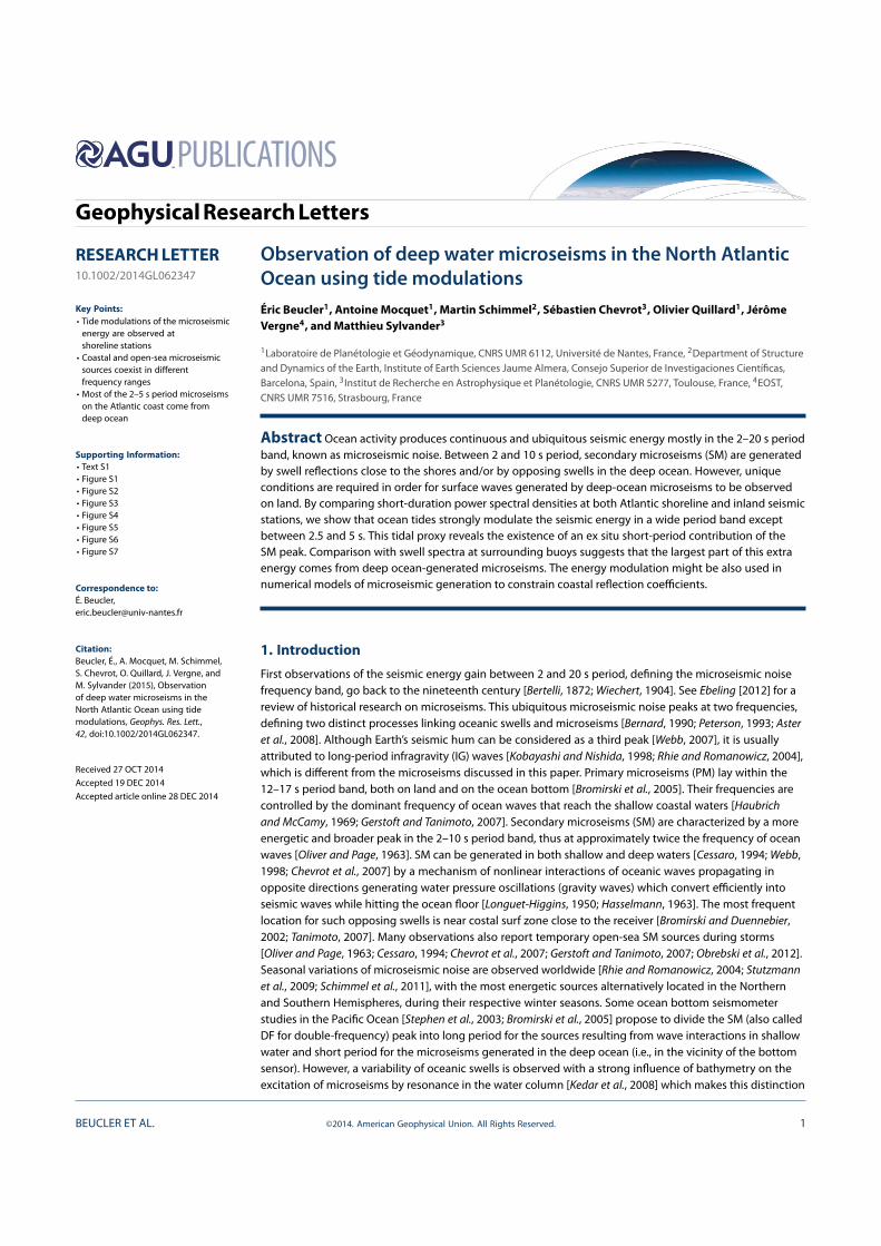
Figure 1. Location of seismic stations and buoys. PY41 and PY48 aretemporary stations deployed less than 150 m from the French Atlantictideline, both on hard rock. VAL station (Irish National Seismic Network)is located about 3 km from the Irish coast and ECH (Geoscope) is takenas a reference inland seismometer. BY (Brittany) and K4 buoys aremaintained by the UK Met Office.

not applicable worldwide. Recent seismicnoise modeling [Ardhuin et al., 2011;Stutzmann et al., 2012; Ardhuin andHerbers, 2013; Sergeant et al., 2013]indicates that coastal reflections can beneglected for periods shorter than 7 s.Both coastal and deep water sourcescan therefore coexist, but some studiesconclude that SM recorded on land aredominated by near-coastal wave activity[Bromirski et al., 2013; Ying et al.,2014]. However, seasonal variabilityleads to a variety of microseismic energydistributions over the frequency range,whatever the distance to the shorelines[Kedar, 2011]. Therefore, finding aproxy to investigate the relationshipsbetween frequency and location ofmicroseism sources may lead to a betterdiscrimination of the different typesof SM. Here we exploit the strong tidemodulations of the seismic energy,previously detected at other places[e.g., Okihiro and Guza, 1995; Thomsonet al., 2006], and we compareobservations of continuous microseismicsignals recorded at both coastal andinland stations.

Two of the four broadband seismic stations (PY41 and PY48) considered in this study were deployed duringthe 3 year PYRenean Observational Portable Experiment (PYROPE) experiment [Chevrot et al., 2014]. Theywere both installed on hard rock, less than 150 m inland from the tideline (Figure 1). PY41 was located insidea seventeenth century citadel surrounded by a quiet tidal bay, while PY48 was installed inside a blockhausof the second world war, built on a sandstone cliff. The tide along this coast is mostly semidiurnal [Llubeset al., 2008; Fund et al., 2012] with large tidal ranges of approximately 0.5–6.5 m. VAL is a permanent broad-band station in the Irish network, Southwest coast of Ireland, 3 km inland. The tidal range at the nearestshore is smaller (1–3.5 m). The Geoscope station ECH [Romanowicz et al., 1984], about 750 km away fromthe Atlantic Ocean, is taken as a reference as a typical inland station. Two UK Met Office buoys located in thenorthern Atlantic are also used (Figure 1). Brittany (hereafter referred to as BY) and K4 buoys are located inthe deep ocean above approximately 2260 m and 2950 m of water height, respectively. Their distance fromthe nearest shores are of 180 km for K4 and 310 km for BY.

2. Short-Duration Power Spectral Densities

For each seismic station component short-duration power spectral densities (PSDs) are computed in the0.2–70 s period band. We preprocess the time series by cutting the continuous signal into 360 s lengthtime windows, with an overlap of 60 s. After removing the instrument response each record is transformedto acceleration between 10 mHz and 10 Hz. A Fourier transform algorithm is used to convert energyinto 10 log10((m∕s2)2∕Hz), which is equivalent to decibel. The final PSD values are computed by takingthe median of four successive power spectra, which gives a measure of seismic power every 20 min.Comparisons with standard PSD packages assess the data processing quality [McNamara and Boaz, 2006].Since earthquakes are not removed, they produce spikes visible for the whole frequency band at allstations. The spectrograms of the vertical components are displayed in Figure 2, for a time window runningfrom 12 to 29 April 2012. Locally predicted tidal ranges, computed by the French Naval Hydrographicand Oceanographic Service, are superimposed on the PY41 and PY48 spectrograms. The correspondingspectrograms for the horizontal components are displayed in Figures S1 and S2 in the supporting



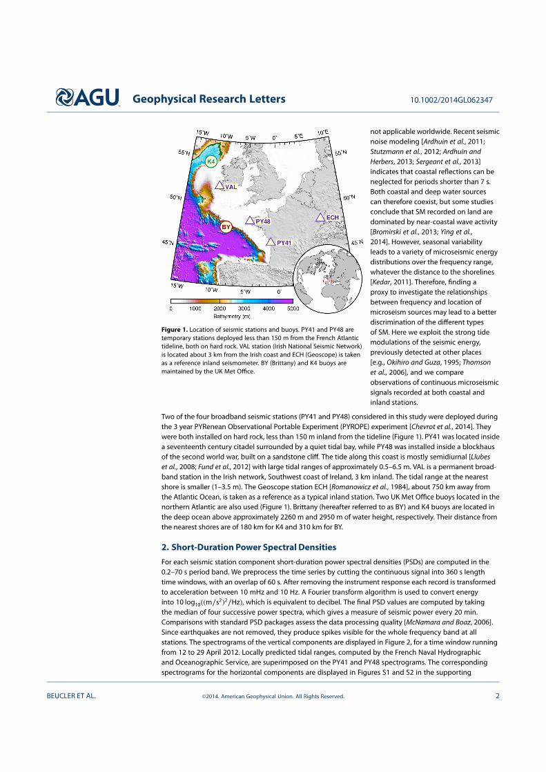
Figure 2. Vertical short-duration power spectrograms during 17 days in April 2012. Periods and frequencies are plottedon the horizontal axes (bottom and top, respectively). PSD are computed between 0.2 and 70 s period. No data selectionhas been performed to remove earthquakes. The local tidal ranges at PY41 and PY48 are represented by magentacurves on the right. The wave heights at Brittany (BY) and K4 buoys (Figure 1) are plotted in brown and green,respectively. The dashed lines highlight some noticeable wave events discussed in the text.

information. For the sake of clarity, we denote hereafter the 2.5–5 s and 5–10 s period bands as SPSM andLPSM (for short- and long-period secondary microseisms, respectively).

The three coastal stations exhibit a larger noise level than the inland station (ECH), especially in the SPSMband, which is significantly wider. For instance, the PSD differences between PY48 and ECH, averaged overthe month of April 2012, amount to 13.2 dB at 3 s period, whereas they do not exceed 4 dB at 7.5 s period.We notice a strong correlation between wave height peaks (dashed lines, Figure 2) and the shape of theSM peak with a broadening toward long periods during storm episodes (time labels B to E). The few hourdelays between the wave height maxima and the increases of both period and energy correspond to thetime taken by swells to travel the distance from the buoys to the nearest shores. The energy in the 12–18s period band (PM peak) increases in concert with ocean swell arrivals on coasts and so with the samedelay times. The very short period energy variations (0.2–2 s), observed also with the same delay times, areconsistent with breaking waves at local shorelines. The broadenings of SM energy toward long periodscan thus be explained by “wave-wave” interactions in shallow waters, which is consistent with near-shoreswell spectra as shown in Figure S3a. The identification of LPSM microseisms on Irish coasts near VAL (timelabel B, Figure 2) and 12 h later on Brittany shorelines near PY48 (time label C) is representative of the stormmigration. At the onset of time label B, the seismometers are observing the formation of the swell inthe fetch, in which short wind generated waves become progressively longer. Few hours later, the swellpropagation toward the coasts induces the typical linear dispersion from long to short waves, as previouslyshown by Chevrot et al. [2007] and Kedar [2011]. This behavior is supported by the numerical wave modelsprovided by Previmer project (see the Acknowledgments section). On the other hand, moderate waveheight peaks (such as time label A) do not necessarily reach the shores and consequently do not producenoticeable LPSM patterns while they are visible in the SPSM window nevertheless. Viewed from ECH,wave-wave interactions at distant coasts (1300 km and 900 km for VAL and PY48, respectively) produce two



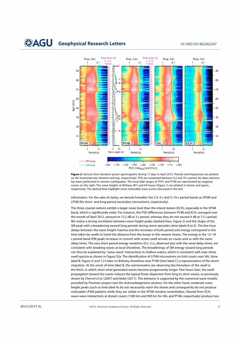
Figure 3. Energy of power spectral density modulations by theprincipal semidiurnal tidal component M2. PSD time seriesof 225 days (10 April to 23 November 2012) are used in thiscomputation. No normalization is applied.

very similar LPSM broadenings, theshort-period energy is largely attenuated.The previous interpretations might bequestioned, since SM frequencies dependon swell spectra, bathymetry, and existenceof opposing waves, which is not easy tobe proved when using isolated buoy datasets. We thus look for additional evidencesusing the strong cyclic pattern that is visibletwice a day, and perfectly synchronizedwith local tidal range oscillations at bothPY41 and PY48. High tides coincide withan increase of microseismic energy over alarge spectral bandwidth and conversely,at low tides, the noise reaches minimumamplitude. At PY41 for instance, PSD valuesincrease up to 20 dB at a 14 s period (greencurve in Figure S4a). The microseismic noiseat this station strongly depends on varioustidal components, including shallow water

harmonics. The same semidiurnal stripes are visible on the PY48 spectrogram with smaller and largermodulations at long and short periods, respectively. The horizontal spectrograms (Figures S1 and S2)show that tides (especially M2 component) modulate the three-component microseismic energy between0.2 s and 70 s period. While tidal modulations of the seismic signal have been previously studied mostly forIG energy [e.g., Dolenc et al., 2005; Young et al., 2013], we report here observations of such modulations inthe microseismic 2–20 s period band. A striking feature of all spectrograms is the lack of semidiurnal stripesin the SPSM band, indicating that the high-and-low tidal cyclic modulations are extremely weak. So, sincecoastal microseismic sources are expected to be influenced by the tides, a distant and larger energy eclipseslocal tidal imprints in this spectral band.

3. M2 Tidal Peak Modulations

The well-known 24 h modulation of the cultural noise can be superimposed on the tidal modulation, whichcontributes to the S1 and S2 peaks, as observed in Figure S4 for PY41. For this reason and because thesemidiurnal M2 tide is known to be the most energetic tidal component, we focus our tidal analysis onthe seismic energy modulation at the M2 frequency (∼1.9323 cpd). For each station, M2 modulationcurves, shown in Figure 3, are computed for each component between 10 April and 23 November 2012(225 days of continuous signal). For each period of the spectrograms shown in Figures 2, S1, and S2, thecorresponding PSD values are extracted as a function of time, with a sampling rate of 0.8333 mHz (1 pointevery 20 min). Four PSD time series, extracted at four periods, are shown as example in Figure S4a forthe vertical component at PY41. The corresponding spectral amplitudes (Figure S4b) then quantify themodulation energies of each PSD time series. In this example, it is clear that the PSD time series at 3 s(magenta curve) is not affected by the M2 frequency, while the three other time series (extracted at 0.43,14, and 50 s) are strongly modulated by at least two tidal peaks (M2, S2, and/or N2 and other shallow watercomponents). The M2 modulation curves displayed in Figure 3 are constructed by computing themodulation energy at the nearest frequency from M2 for each PSD time series defined between 0.2 and 70 s.No normalization of the modulation amplitude is applied in Figure 3. For the sake of comparison, normalizedcurves are displayed in Figure S5 and show the same behavior at coastal stations.

PSD time series at both VAL and ECH are weakly modulated by the M2 frequency, with respect to PY41 andPY48 (Figure 3), although a similar V shape (with a minimum between 2 and 7 s period) can be noticed forVAL in Figure S5. Conversely, the PSD modulation curves at PY41 and PY48, both very close to the shore,confirm a large M2 modulation of the seismic energy. At PY41, the spectrum enhances that energy dependsnot only on M2 but also on various shallow water tidal components (such as M4, see Figure S4b). At PY48,the short-period modulations (lower than 1 s) can be explained by the energy of ocean waves hitting thecliff at high tides. This modulation of the short-period seismic energy is larger than the effect of the swash at



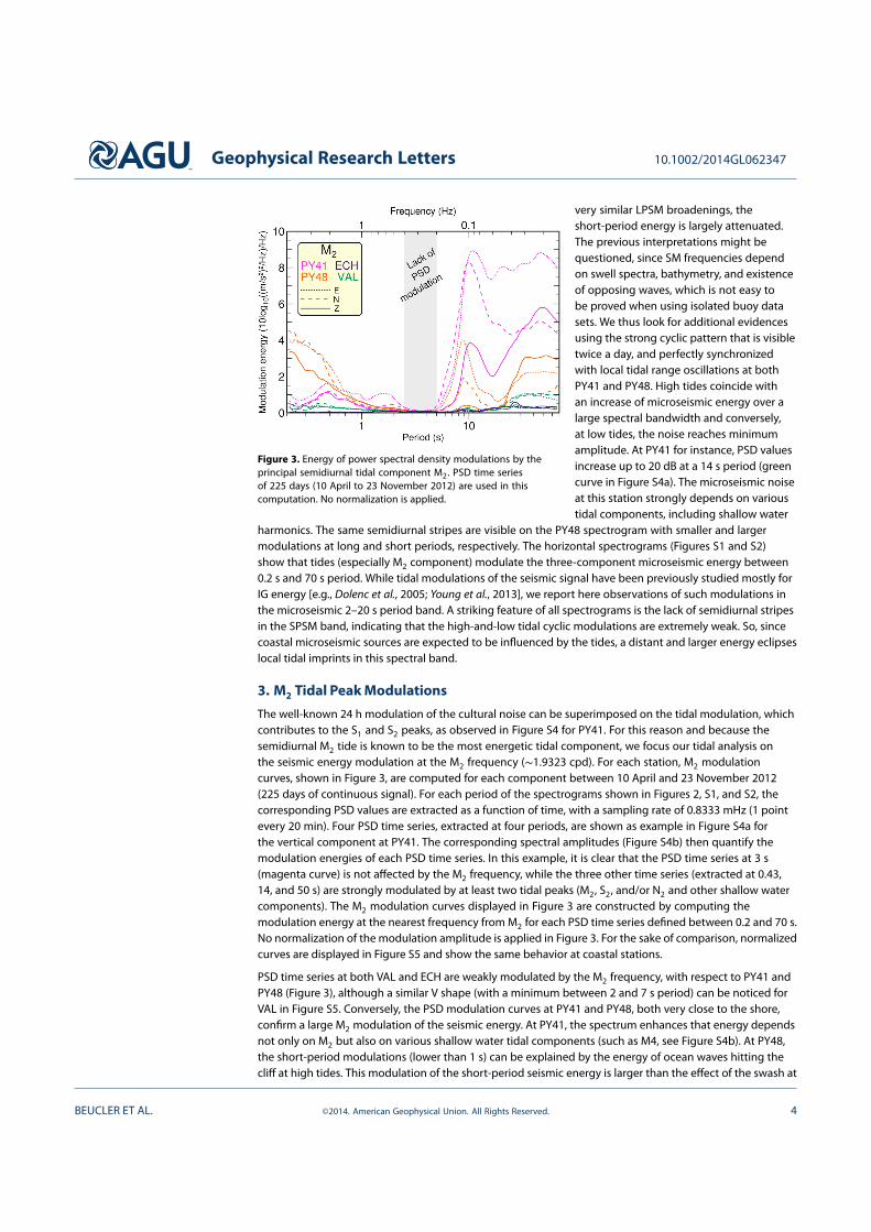
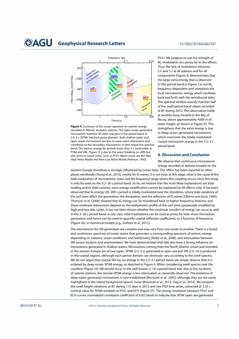
Figure 4. Summary of the ocean signature on seismic energyrecorded at Atlantic shoreline stations. The open ocean-generatedmicroseisms outshine all other energies in the period band of2.5–5 s (SPSM, hatched green domain). Both shallow water andopen ocean microseisms are due to wave-wave interactions andcontribute to the secondary microseisms in their respective spectralband. The seismic energy for periods lower than 2 s (noticeable atPY48 and VAL, Figure 2) is due to the wave breaking on cliffs butalso exists in swash areas, such as PY41. Black curves are the NewHigh Noise Model and New Low Noise Model [Peterson, 1993].

PY41. We propose to use the strength ofM2 modulation as a proxy for in situ effects.Thus, the lack of modulation between2.5 and 5 s at all stations and for allcomponents (Figure 3) demonstrates thatthe large extra energy that is observedin this period band in Figure 2 is not M2

frequency dependent and overprints thelocal microseismic energy which oscillatesback and forth with the semidiurnal tides.This spectral window exactly matches halfof the swell period band values recordedat BY during 2012. This observation holdsat another buoy located in the Bay ofBiscay, above approximately 4560 m ofwater height, as shown in Figure S3. Thisstrengthens that the extra energy is dueto deep ocean-generated microseismswhich overcome the tidally modulatedcoastal microseism energy in the 2.5–5 speriod band.

4. Discussion and Conclusion

We observe that continuous microseismicenergy recorded at stations located on the

western Europe shorelines is strongly influenced by ocean tides. This effect has been reported at otherplaces worldwide [Young et al., 2013], mostly for IG waves. It is not clear, at this stage, what is the cause of thetidal modulation of microseismic noise and the frequency range where this coupling occurs since this studyis only focused on the 0.2–20 s period band. So far, we believe that the most likely explanations are tidalloading and/or tidal currents, since energy amplification cannot be explained by tilt effects only. It has beenobserved that IG energy (20–200 s period) is tidally modulated near the shorelines, where tidal variations ofthe surf zone affect the generation, the dissipation, and the reflection of IG waves [Okihiro and Guza, 1995].Thomson et al. [2006] showed that IG energy can be transferred back to higher-frequency motions, andthese nonlinear interactions depend on the bathymetric profile of the surf zone, perpetually modified byhigh-and-low tide cycles. It has not been shown whether this nonlinear transfers of energy can occur as wellin the 2–20 s period band. In any case, tidal modulations can be used as proxy for near-shore microseismgeneration and hence can be used to quantify coastal reflection coefficients, as a function of frequency(Figure S6), in numerical models [e.g., Ardhuin et al., 2011].

The mechanisms for SM generation are complex and may vary from one ocean to another. There is a broadand continuous spectrum of ocean waves that generates a corresponding spectrum of seismic energydepending on seasons, ocean conditions and bathymetry [Kedar et al., 2008], and attenuation betweenSM source location and seismometers. We have demonstrated that tide also have a strong influence onmicroseisms generated in shallow waters. Microseisms coming from the North Atlantic ocean and recordedin the western Europe are of two types: SPSM (2.5–5 s) generated in open sea and SM (2.5–10 s) producedin the coastal regions, although each period domain can obviously vary according to the swell spectra.We do not argue that coastal SM has no energy in the 2.5–5 s period band, we simply observe that it iseclipsed by deep-ocean SPSM energy, as sketched in Figure 4. When considering swell spectra near thecoastline (Figure S3) SM should occur in the well-known 2–10 s period band, but, due to the locationsof seismic stations, the remote SPSM energy is less attenuated, as classically observed. The existence ofdeep water-generated microseisms is now established [Bromirski et al., 2005], although they are not easilyhighlighted in the inland background seismic noise [Bromirski et al., 2013; Ying et al., 2014]. We comparethe swell height variations at BY during 115 days in 2012 and two PSD time series, extracted at 3.33 s(central value for SPSM window) at PY41 and ECH (Figure S7). The strong correlation between PY41 andECH curves (normalized correlation coefficient of 0.92) tends to indicate that SPSM open sea-generated



microseisms are detectable 700 km away from the coast, but with a larger attenuation of the energyduring propagation in the continental crust. At places where such SPSM exist, both coastal and inlandseismometers can find usefulness for presatellite ocean activity reconstruction. Ambient noiseseismology can also benefit from this result for both tomography and monitoring purposes [Shapiroet al., 2005; Brenguier et al., 2008], since the origin of noise sources can influence the cross-correlationreconstruction. Finally, this observation may also contribute to map the opposing wave locations in thecase of storms migrating toward shorelines, using coastal seismometers, in addition to buoy and satellitedata and so to estimate the storm power. For instance, observations of microseismic signals in Florida(station O62Z, see Figure 3 in Sufri et al. [2014]), clearly display short-period microseisms generated bysuperstorm Sandy at late 21 October 2012. If SPSM overprint also exists in the central western AtlanticOcean, the noticeable energy in the 2.5–5 s can be linked to deep-ocean activity which occurred a fewhours before the National Hurricane Center upgraded Sandy as a tropical storm.

ReferencesArdhuin, F., and H. C. Herbers (2013), Noise generation in the solid earth, oceans and atmosphere, from nonlinear interacting surface

gravity waves in finite depth, J. Fluid Mech., 716, 316–348.Ardhuin, F., E. Stutzmann, M. Schimmel, and A. Mangeney (2011), Ocean wave sources of seismic noise, J. Geophys. Res., 116, C09004,

doi:10.1029/2011JC006952.Aster, R. C., D. E. McNamara, and P. D. Bromirski (2008), Multidecadal climate-induced variability in microseisms, Seismol. Res. Lett., 79(2),

194–202, doi:10.1785/gssrl.79.2.194.Bernard, P. (1990), Historical sketch of microseisms from past to future, Phys. Earth Planet. Inter., 63(3–4), 145–150.Bertelli, T. (1872), Osservazioni sui piccoli movimenti dei pendoli in relazione ad alcuni fenomeni meteorologiche, Boll. Meteorol. Osserv.

Coll. Roma, 9, 19.Brenguier, F., N. Shapiro, M. Campillo, V. Ferrazzini, Z. Duputel, O. Coutant, and A. Nercessian (2008), Towards forecasting volcanic

eruptions using seismic noise, Nat. Geosci., 1(2), 126–130.Bromirski, P. D., and F. K. Duennebier (2002), The near-coastal microseism spectrum: Spatial and temporal wave climate relationships,

J. Geophys. Res., 107(B8), 2166, doi:10.1029/2001JB000265.Bromirski, P. D., F. K. Duennebier, and R. A. Stephen (2005), Mid-ocean microseisms, Geochem. Geophys. Geosyst., 6, Q04009,

doi:10.1029/2004GC000768.Bromirski, P. D., R. A. Stephen, and P. Gerstoft (2013), Are deep-ocean-generated surface-wave microseisms observed on land?, J. Geophys.

Res. Solid Earth, 118, 3610–3629, doi:10.1002/jgrb.50268.Cessaro, R. K. (1994), Sources of primary and secondary microseisms, Bull. Seismol. Soc. Am., 84(1), 142–148.Chevrot, S., M. Sylvander, S. Benahmed, C. Ponsolles, J. M. Lefèvre, and D. Paradis (2007), Source locations of secondary microseisms in

western Europe: Evidence for both coastal and pelagic sources, J. Geophys. Res., 112, B11301, doi:10.1029/2007JB005059.Chevrot, S., et al. (2014), High-resolution imaging of the Pyrenees and Massif Central from the data of the PYROPE and IBERARRAY

portable array deployments, J. Geophys. Res. Solid Earth, 119, 6399–6420, doi:10.1002/2014JB010953.Dolenc, D., B. Romanowicz, D. Stakes, P. McGill, and D. Neuhauser (2005), Observations of infragravity waves at the Monterey ocean

bottom broadband station (MOBB), Geochem. Geophys. Geosyst., 6, Q09002, doi:10.1029/2005GC000988.Ebeling, C. W. (2012), Chapter one—Inferring ocean storm characteristics from ambient seismic noise: A historical perspective,

in Advances in Geophysics, vol. 53, edited by R. Dmowska, pp. 1–33, Elsevier.Frigo, M., and S. G. Johnson (2005), The design and implementation of FFTW3, Proc. IEEE, 93(2), 216–231, special issue on “Program

Generation, Optimization, and Platform Adaptation”.Fund, F., L. Morel, and A. Mocquet (2012), Assessment of the FES2004 derived OTL model in the west of France and preliminary

results about impacts of tropospheric models, in Geodesy for Planet Earth, International Association of Geodesy Symposia,vol. 136, edited by S. Kenyon, M. C. Pacino, and U. Marti, pp. 573–579, Springer, Berlin, doi:10.1007/978-3-642-20338-1_70.

Gerstoft, P., and T. Tanimoto (2007), A year of microseisms in southern California, Geophys. Res. Lett., 34, L20304,doi:10.1029/2007GL031091.

Hasselmann, K. (1963), A statistical analysis of the generation of microseisms, Rev. Geophys., 1(2), 177–210.Haubrich, R., and K. McCamy (1969), Microseisms: Coastal and pelagic sources, Rev. Geophys., 7, 539–571.Kedar, S. (2011), Source distribution of ocean microseisms and implications for time-dependent noise tomography, C. R. Geosci., 343(8–9),

548–557.Kedar, S., M. Longuet-Higgins, F. Webb, N. Graham, R. Clayton, and C. Jones (2008), The origin of deep ocean microseisms in the north

Atlantic ocean, Proc. R. Soc. A, 464(2091), 777–793, doi:10.1098/rspa.2007.0277.Kobayashi, N., and K. Nishida (1998), Continuous excitation of planetary free oscillations by atmospheric disturbances, Nature, 395,

357–360, doi:10.1038/2642.Llubes, M., et al. (2008), Multi-technique monitoring of ocean tide loading in northern France, C. R. Geosci., 340(6), 379–389.Longuet-Higgins, M. S. (1950), A theory of the origin of microseisms, Philos. Trans. R. Soc. London, 243(857), 1–35.McNamara, D. E., and R. Boaz (2006), Seismic noise analysis system using power spectral density probability density functions:

A stand-alone software package, U.S. Geol. Surv. Open File Rep., 2005–1438.Obrebski, M. J., F. Ardhuin, E. Stutzmann, and M. Schimmel (2012), How moderate sea states can generate loud seismic noise in the

deep ocean, Geophys. Res. Lett., 39, L11601, doi:10.1029/2012GL051896.Okihiro, M., and R. T. Guza (1995), Infragravity energy modulation by tides, J. Geophys. Res., 100(C8), 16,143–16,148.Oliver, J., and R. Page (1963), Concurrent storms of long and ultralong period microseisms, Bull. Seismol. Soc. Am., 53(1), 15–26.Peterson, J. (1993), Observations and modelling of seismic background noise, U.S. Geol. Surv. Open File Rep., 93 –322.Rhie, J., and B. Romanowicz (2004), Excitation of Earth’s continuous free oscillations by atmosphere ocean seafloor coupling, Nature,

431, 552–556.

AcknowledgmentsThe Atlantic station deploymentwould not have been possible with-out the help of the municipalitiesof Camaret-sur-mer (PY48) andLe-Château-d’Oléron (PY41). ThePYROPE data set is archived by Geo-data team of ISTerre (Grenoble). PY41and PY48 are now RESIF permanentstations (UNCO and CAMF, respec-tively), and data are freely available(http://www.resif.fr). ECH is a Geo-scope station, and authors would liketo thank Sergei Lebedev for provid-ing VAL continuous data. Figures areproduced using GMT [Wessel et al.,2013], and our data processingcodes use “The Fastest Fourier Trans-form of the West” [Frigo and Johnson,2005] libraries. The buoy data werecollected and made freely availableby the CDOCO in the framework ofPrevimer project and programs thatcontribute to it (http://www.previmer.org). This work is supported by theANR-09-0229-000 (PYROPE project),VIBRIS project (Council of Pays de laLoire), and by the Nantes-AtlantiqueObservatory (OSUNA). M. Schimmelacknowledges support byTopoIberia (CSD2006-00041) andCGL2013-48601-C2-1-R. We would liketo thank the Editor, an anonymousreviewer, and Sharon Kedar for veryconstructive comments. In memoryof Olivier Quillard who installed andmaintained PYROPE stations.

The Editor thanks two anonymousreviewers for their assistance inevaluating this paper.



Romanowicz, B., M. Cara, J.-F. Fels, and D. Rouland (1984), Geoscope: A French initiative in long period three component seismicnetworks, Eos Trans. AGU, 65, 753–754.

Schimmel, M., E. Stutzmann, F. Ardhuin, and J. Gallart (2011), Polarized Earth’s ambient microseismic noise, Geochem. Geophys. Geosyst.,12, Q07014, doi:10.1029/2011GC003661.

Sergeant, A., E. Stutzmann, A. Maggi, M. Schimmel, F. Ardhuin, and M. Obrebski (2013), Frequency-dependent noise sources in the northAtlantic Ocean, Geochem. Geophys. Geosyst., 14, 5341–5353, doi:10.1002/2013GC004905.

Shapiro, N. M., M. Campillo, L. Stehly, and M. H. Ritzwoller (2005), High-resolution surface-wave tomography from ambient seismic noise,Science, 307(5715), 1615–1618, doi:10.1126/science.1108339.

Stephen, R. A., F. N. Spiess, J. A. Collins, J. A. Hildebrand, J. A. Orcutt, K. R. Peal, F. L. Vernon, and F. B. Wooding (2003), Ocean seismicnetwork pilot experiment, Geochem. Geophys. Geosyst., 4(10), 1092, doi:10.1029/2002GC000485.

Stutzmann, E., M. Schimmel, G. Patau, and A. Maggi (2009), Global climate imprint on seismic noise, Geochem. Geophys. Geosyst., 10,Q11004, doi:10.1029/2009GC002619.

Stutzmann, E., F. Ardhuin, M. Schimmel, A. Mangeney, and G. Patau (2012), Modelling long-term seismic noise in various environments,Geophys. J. Int., 191(2), 707–722, doi:10.1111/j.1365-246X.2012.05638.x.

Sufri, O., K. D. Koper, R. Burlacu, and B. de Foy (2014), Microseisms from superstorm Sandy, Earth Planet. Sci. Lett., 402, 324–336, specialissue on {USArray} science.

Tanimoto, T. (2007), Excitation of microseisms, Geophys. Res. Lett., 34, L05308, doi:10.1029/2006GL029046.Thomson, J., S. Elgar, B. Raubenheimer, T. H. C. Herbers, and R. T. Guza (2006), Tidal modulation of infragravity waves via nonlinear energy

losses in the surfzone, Geophys. Res. Lett., 33, L05601, doi:10.1029/2005GL025514.Webb, S. C. (1998), Broadband seismology and noise under the ocean, Rev. Geophys., 36(1), 105–142, doi:10.1029/97RG02287.Webb, S. C. (2007), The Earth’s “hum” is driven by ocean waves over the continental shelves, Nature, 445, 754–756,

doi:10.1038/nature05536.Wessel, P., W. H. F. Smith, R. Scharroo, J. Luis, and F. Wobbe (2013), Generic Mapping Tools: Improved version released, Eos Trans. AGU,

94(45), 409–410, doi:10.1002/2013EO450001.Wiechert, E. (1904), Verhandlugen der zweiten internationalen seismologischen konferenz, Gerlands Beitr. Geophys., 2, 41–43.Ying, Y., C. J. Bean, and P. D. Bromirski (2014), Propagation of microseisms from the deep ocean to land, Geophys. Res. Lett., 41, 6374–6379,

doi:10.1002/2014GL060979.Young, A. P., R. T. Guza, M. E. Dickson, W. C. O’Reilly, and R. E. Flick (2013), Ground motions on rocky, cliffed, and sandy shorelines

generated by ocean waves, J. Geophys. Res. Oceans, 118, 6590–6602, doi:10.1002/2013JC008883.


Documents

Observation of deep water microseisms in the North Atlantic Ocean using tide modulations