The Astrophysical Journal, 799:220 (11pp), 2015 February 1 doi:10.1088/0004-637X/799/2/220C© 2015. The American Astronomical Society. All rights reserved.

OBSERVATIONS AND MODELING OF NORTH–SOUTH ASYMMETRIESUSING A FLUX TRANSPORT DYNAMO

Juie Shetye1, Durgesh Tripathi2, and Mausumi Dikpati31 Armagh Observatory, College Hill, Armagh City BT61 9DG, UK

2 Inter-University Centre for Astronomy and Astrophysics, Post Bag 4, Ganeshkhind, Pune 411007, India3 High Altitude Observatory, National Center for Atmospheric Research, Boulder, CO 80307, USA

Received 2014 January 23; accepted 2014 December 9; published 2015 January 30

ABSTRACT

The peculiar behavior of solar cycle 23 and its prolonged minima has been one of the most studied problems overthe past few years. In the present paper, we study the asymmetries in active region magnetic flux in the northern andsouthern hemispheres during the complete solar cycle 23 and the rising phase of solar cycle 24. During the decliningphase of solar cycle 23, we find that the magnetic flux in the southern hemisphere is about 10 times stronger than thatin the northern hemisphere; however, during the rising phase of cycle 24, this trend is reversed. The magnetic fluxbecomes about a factor of four stronger in the northern hemisphere than in the southern hemisphere. Additionally,we find that there was a significant delay (about five months) in change of the polarity in the southern hemispherein comparison with the northern hemisphere. These results provide us with hints of how the toroidal fluxes havecontributed to the solar dynamo during the prolonged minima in solar cycle 23 and in the rising phase of solarcycle 24. Using a solar flux-transport dynamo model, we demonstrate that persistently stronger sunspot cyclesin one hemisphere could be caused by the effect of greater inflows into active region belts in that hemisphere.Observations indicate that greater inflows are associated with stronger activity. Some other change or difference inmeridional circulation between hemispheres could cause the weaker hemisphere to become the stronger one.

Key words: Sun: activity – Sun: magnetic fields – Sun: photosphere – sunspots

1. INTRODUCTION

Based on the observations of sunspots on the surface ofthe Sun and the relatively well organized poloidal field, whichchanges polarity approximately every 11 yr, it has been univer-sally accepted that the solar magnetic cycle is a dynamo processinvolving the transformation of the polar field into the toroidalfield and subsequent conversion of the toroidal field into thepoloidal field of opposite polarity over the course of approx-imately 11 yr (see, e.g., Babcock 1961 and its citations). Thegeneration and propagation of large-scale magnetic fields viathe dynamo mechanism are considered to be a two-step process.The first step involves shearing of the poloidal component of themagnetic field by differential rotation, which gives rise to theazimuthally directed toroidal magnetic field. This toroidal fieldthen gives rise to the formation of the sunspots and the activeregions (ARs). The second step is the formation of the poloidalcomponent from the toroidal component, which occurs fromthe magnetic flux being liberated by the growth and the decayof the sunspots, with the leading polarity flux moving towardthe equator and the following polarity toward the pole. In somemodels, movement of the following polarity fields toward polesis due to the meridional circulation, as illustrated with both thekinematic dynamo and flux-transport dynamo models (see, e.g.,Wang et al. 1991; Choudhuri et al. 1995 and references therein).

The study of the solar cycle on long timescales indicatesthat the solar cycle is virtually symmetric between the north-ern and southern hemispheres, in the sense that the averageamplitudes, shapes, and durations of cycles are very similar(see, e.g., Goel & Choudhuri 2009). However, there are indi-vidual cycles that are known to be stronger in one hemispherethan the other. For example, just after the Maunder Minimum,almost all the sunspots were observed in the southern hemi-sphere (see, e.g., Ribes & Nesme-Ribes 1993). Asymmetriesbetween the two hemispheres have also been observed in various

solar activity phenomena such as sunspot area, sunspot numbers,faculae, coronal structure, posteruption arcades, coronal ioniza-tion temperatures, polar field reversals, and solar oscillations(see, e.g., Chowdhury et al. 2013; Sykora & Rybak 2010; Gaoet al. 2009; Li et al. 2009; Temmer et al. 2006; Knaack et al.2004, 2005; Tripathi et al. 2004; Atac & Ozguc 1996; Oliver &Ballester 1994; Zolotova et al. 2010; Svalgaard & Kamide 2013and references therein), in addition to long-term hemisphericasymmetries in solar activity in previous solar cycles (see, e.g.,Vizoso & Ballester 1989; Carbonell et al. 1993; Norton &Gallagher 2010).

Further, the rise and fall of solar cycle 23 has been discussedby many authors; it has been found that the behavior of solarcycle 23 is very peculiar for an odd-numbered cycle (Chowdhuryet al. 2013). Cycle 23 showed a slow rise compared to otherodd-numbered cycles and was found to be weak comparedto other odd-numbered cycles (Li et al. 2009; Chowdhuryet al. 2013). Additionally, it shows an unusual second peakduring the declining phase (Li et al. 2009; Mishra & Mishra2012). Moreover, the temporal characteristics of cycle 23, suchas sunspot number and sunspot area, are similar to those ofthe Gleissberg global minimum cycles 11, 13, and 14, whichoccurred between 1880 and 1930, as well as solar cycle 20(Krainev 2012). Analysis of polar field patterns indicates thatpolar field reversal was slower than in the previous two cycles,as discussed in (Dikpati et al. 2004), which could have delayedthe rise of solar cycle 24. The first two years of cycle 24,with low solar activity concentrated in the south, are similarto the cycle that immediately followed the Maunder Minimum(Krainev 2012).

Our motivation for this research is to investigate solar cycle23 and the rise of solar cycle 24 by computing the AR fluxes thatform the toroidal fluxes. We then concentrate on the solar cycleminimum and investigate the asymmetry in the hemisphereswith the aim of addressing the issue related to the deep minimum

1

The Astrophysical Journal, 799:220 (11pp), 2015 February 1 Shetye, Tripathi, & Dikpati

Figure 1. Position of all the ARs formed between 2005 July 22 and 2010 April 12 during the decline phase of solar cycle 22 (top left), the rise phase of solar cycle 23(top right), the decline phase of solar cycle 23 (bottom left), and the rise phase of cycle 24 (bottom right). The location of the AR is based on its nomenclature fromthe NOAA database.

observed in cycle 23. To support our observations, we havecarried out dynamo simulations as mentioned in Belucz &Dikpati (2013). We also investigated the role of meridionalcirculation combined with flux asymmetry for solar cycle 23 bydiscussing different cases related to the asymmetries found. Therest of the paper is organized as follows. In Section 2 we presentthe observations and data selection, followed by magnetic fluxanalysis and results in Section 3. In Section 4 we discuss dynamosimulations and relate them to our observations. In Section 5 wesummarize the results and science.

2. OBSERVATIONS AND DATA

We calculate the line-of-sight (LOS) component of themagnetic field (hereafter B⊥) using the magnetograms recordedby the Michelson Doppler Imager (MDI; Scherrer et al. 1995)on board the Solar Heliospheric Observatory (SOHO). MDI isan instrument used to observe signs and strength of the LOScomponent of the photospheric magnetic field. MDI images theSun using a 1024 × 1024 CCD camera and acquires one full-disk LOS magnetic field each 96 minutes (5 minutes averagedmagneto grams), among other observing sequences, which is

free from atmospheric noise. A full-disk magnetogram of theSun has a resolution of ∼4′′ (2′′ × 2′′ pixel−1) and a field of viewof 34′ × 34′. Preflight per-pixel error in the flux was estimatedat 20 G (20 Mx cm−2) (Scherrer et al. 1995), which was foundto be 14 G in flight, as was reported by Hagenaar (2001).

In the present work, we have used MDI magnetogramsto compute the daily magnetic flux of ARs observed bysolarmonitor.org on the solar disk from 1996 May 6 to 2010April 12 (approximately 5100 days), which covers the finalstages of solar cycle 22, the complete cycle 23, and the risingphase of cycle 24. During this period, we have manuallymonitored evolution of 1948 ARs, which include 286 AR nestsand 6 AR evolutions, where the dispersion stage of ARs wasobserved to be persistent over multiple revolutions. We preferredusing a manual approach over an automated one, as discussedin Zhang et al. (2010) and Stenflo & Kosovichev (2012), so thatwe could eliminate multiple counting of the same AR due tosolar rotation.

Figure 1 shows the location of ARs on the solar disk duringthe declining phase of cycle 22 (top left), the rising phase of solarcycle 23 (top right), the declining phase of solar cycle 23 (bot-tom left), and the rising phase of solar cycle 24 (bottom right).

2

The Astrophysical Journal, 799:220 (11pp), 2015 February 1 Shetye, Tripathi, & Dikpati

0 500 1000 1500 2000 2500 3000 3500 4000 4500 5000 5500−1000

−800

−600

−400

−200

0

200

400

600

800

1000

Observation of 5162 days

arcs

econ

ds

Butterfly diagram representing AR positions between 1996 May 06 to 2010 April 12

MDIDATALOSS

MDIDATALOSS

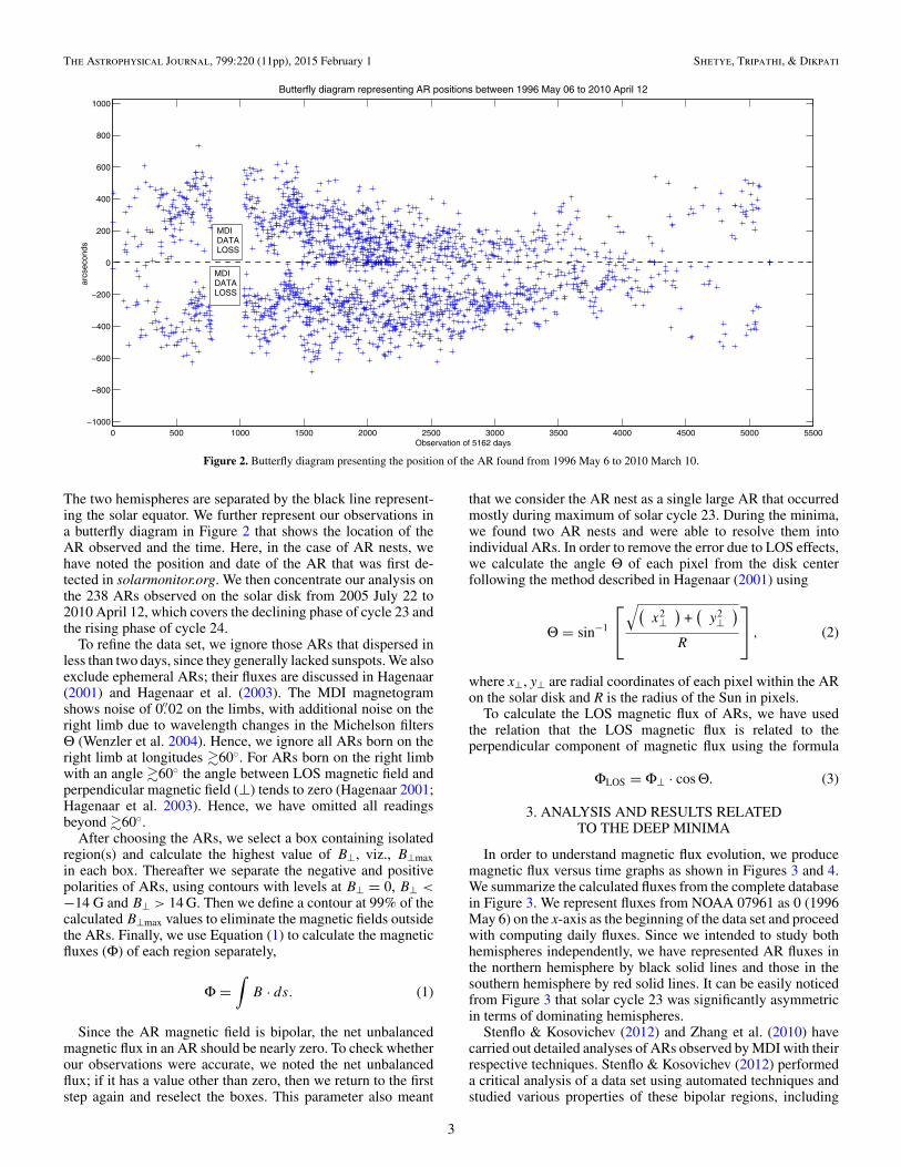
Figure 2. Butterfly diagram presenting the position of the AR found from 1996 May 6 to 2010 March 10.

The two hemispheres are separated by the black line represent-ing the solar equator. We further represent our observations ina butterfly diagram in Figure 2 that shows the location of theAR observed and the time. Here, in the case of AR nests, wehave noted the position and date of the AR that was first de-tected in solarmonitor.org. We then concentrate our analysis onthe 238 ARs observed on the solar disk from 2005 July 22 to2010 April 12, which covers the declining phase of cycle 23 andthe rising phase of cycle 24.

To refine the data set, we ignore those ARs that dispersed inless than two days, since they generally lacked sunspots. We alsoexclude ephemeral ARs; their fluxes are discussed in Hagenaar(2001) and Hagenaar et al. (2003). The MDI magnetogramshows noise of 0.′′02 on the limbs, with additional noise on theright limb due to wavelength changes in the Michelson filtersΘ (Wenzler et al. 2004). Hence, we ignore all ARs born on theright limb at longitudes �60◦. For ARs born on the right limbwith an angle �60◦ the angle between LOS magnetic field andperpendicular magnetic field (⊥) tends to zero (Hagenaar 2001;Hagenaar et al. 2003). Hence, we have omitted all readingsbeyond �60◦.

After choosing the ARs, we select a box containing isolatedregion(s) and calculate the highest value of B⊥, viz., B⊥maxin each box. Thereafter we separate the negative and positivepolarities of ARs, using contours with levels at B⊥ = 0, B⊥ <−14 G and B⊥ > 14 G. Then we define a contour at 99% of thecalculated B⊥max values to eliminate the magnetic fields outsidethe ARs. Finally, we use Equation (1) to calculate the magneticfluxes (Φ) of each region separately,

Φ =∫

B · ds. (1)

Since the AR magnetic field is bipolar, the net unbalancedmagnetic flux in an AR should be nearly zero. To check whetherour observations were accurate, we noted the net unbalancedflux; if it has a value other than zero, then we return to the firststep again and reselect the boxes. This parameter also meant

that we consider the AR nest as a single large AR that occurredmostly during maximum of solar cycle 23. During the minima,we found two AR nests and were able to resolve them intoindividual ARs. In order to remove the error due to LOS effects,we calculate the angle Θ of each pixel from the disk centerfollowing the method described in Hagenaar (2001) using

Θ = sin−1

⎡⎣

√(x2

⊥)

+(

y2⊥

)R

⎤⎦ , (2)

where x⊥, y⊥ are radial coordinates of each pixel within the ARon the solar disk and R is the radius of the Sun in pixels.

To calculate the LOS magnetic flux of ARs, we have usedthe relation that the LOS magnetic flux is related to theperpendicular component of magnetic flux using the formula

ΦLOS = Φ⊥ · cos Θ. (3)

3. ANALYSIS AND RESULTS RELATEDTO THE DEEP MINIMA

In order to understand magnetic flux evolution, we producemagnetic flux versus time graphs as shown in Figures 3 and 4.We summarize the calculated fluxes from the complete databasein Figure 3. We represent fluxes from NOAA 07961 as 0 (1996May 6) on the x-axis as the beginning of the data set and proceedwith computing daily fluxes. Since we intended to study bothhemispheres independently, we have represented AR fluxes inthe northern hemisphere by black solid lines and those in thesouthern hemisphere by red solid lines. It can be easily noticedfrom Figure 3 that solar cycle 23 was significantly asymmetricin terms of dominating hemispheres.

Stenflo & Kosovichev (2012) and Zhang et al. (2010) havecarried out detailed analyses of ARs observed by MDI with theirrespective techniques. Stenflo & Kosovichev (2012) performeda critical analysis of a data set using automated techniques andstudied various properties of these bipolar regions, including

3

The Astrophysical Journal, 799:220 (11pp), 2015 February 1 Shetye, Tripathi, & Dikpati

0 500 1000 1500 2000 2500 3000 3500 4000 4500 5000 55000

0.5

1

1.5

2

2.5

3x 10

25

Observations of 5162 days

Mag

netic

flux

in M

xAR fluxes covering solar cycle 23 and rising phase of solar cycle 24 (total data from 1996 May 06 to 2010 April 12)

Northern Hemisphere

Southern Hemisphere

MDIdataloss

Risingphase ofcycle 24Deep

minimum

Decliningphase ofcycle 23

Maximum ofcycle 23

Figure 3. Comparison of AR flux behavior between the northern and the southern hemispheres from 1996 May 6 to 2010 March 10.

their orientation and the tilt angle variation. Zhang et al. (2010),on the other hand, studied the basic physical parameters, includ-ing the magnetic flux of individual ARs and their distributionwith respect to size as well as magnetic flux. They found thesolar cycle between 1996 and 2008 to be very asymmetric. Interms of number of ARs, they found 938 ARs in the south and792 in the north. We found similar results: we found 1071 ARsin the south and 872 in the north, which makes the asymme-try approximately 12%. Zhang et al. (2010) also studied theasymmetry in the magnetic flux and found that the southernhemisphere was stronger than the northern hemisphere duringthe declining phase of solar cycle 23; we found a similar asym-metry, where we found 10 times more flux emergence in thesouthern hemisphere. These results are also in agreement withthose obtained by (Li et al. 2009) and (Chowdhury et al. 2013),based on sunspot observations.

Figure 3 suggests that the behavior of deep minima maybe related to AR fluxes related to the later part of the decliningphase of cycle 23. Thus, we concentrate our analysis on the latterpart of cycle 23. In order to study the flux behavior therein, weselected the final 1694 days from Figure 3 (i.e., data between the3468th day and the 5162th day) and represented in the graphsin Figure 4. Here we represent our observations with NOAAAR 10791 (northern hemisphere, observed on 2005 July 22 andrepresented by 0 on the x-axis in the top panel of Figure 4). In thesouth we began with NOAA AR 10794 (southern hemisphere,observed on 2005 August 1), both occurring roughly midwayduring the declining phase of cycle 23. We continue until thedispersion of NOAA AR 11060 (in the northern hemisphere on2010 April 12, represented by 1694 on the x-axis in Figure 4) inthe north. In the plots, the blue line indicates the magnetic fluxbehavior during the declining phase of cycle 23, and the blackline indicates the magnetic flux behavior during the rising phaseof cycle 24.

Figure 4 clearly indicates that photospheric magnetic fluxduring the final four years of solar cycle 23 was dominant

in the southern hemisphere, producing a profound north–southasymmetry in terms of AR numbers and magnetic flux. Duringthis period, we found 121 ARs in the southern hemisphere ascompared to 60 ARs in the northern hemisphere. This asym-metry becomes even more pronounced as the cycle progresses.The AR fluxes in the southern hemisphere were approximately10 times stronger than those in the northern hemisphere. But thisbehavior changed completely during the rising phase of cycle24, for which the strength of fluxes in the north is four timesthat in the south. This was observed with 36 ARs emergingin the north compared to 23 in the south. Proceeding towardcycle 24, we find that (see Figure 4) the new cycle began inthe north on the 875th day, which is 2007 December 13, whenthe emergence of an opposite polarity sunspot was observed.In the south the opposite polarity sunspot was observed on the1013th day, which is 2008 May 3. This is 143 days (about fivemonths) after the reversal of polarities in the northern hemi-sphere. Moreover, Figure 4 also clearly shows that the changeof polarity in the northern hemisphere occurred smoothly andquickly, with a mixture of ARs from both cycles for a period of200 days, whereas in the southern hemisphere, the new emerg-ing flux showed a delay.

4. NORTH–SOUTH ASYMMETRIESFROM DYNAMO ACTION

In order to understand how the solar dynamo works and toinvestigate the reason behind our observational results con-cerning the asymmetry between hemispheres, as well as tounderstand the effect of this asymmetry on the deep minima,we have carried out sets of dynamo simulations. Belucz &Dikpati (2013) have shown that differences in the form and am-plitude of meridional circulation between northern and southernhemispheres can cause significant differences in the poloidal,polar, and toroidal fields produced there. The longer the merid-ional circulation differences persisted, the larger the differencesbecame. Belucz & Dikpati (2013) focused on global changes

4

The Astrophysical Journal, 799:220 (11pp), 2015 February 1 Shetye, Tripathi, & Dikpati

0 200 400 600 800 1000 1200 1400 1600 18000

0.5

1

1.5

2

2.5

3

3.5x 10

24

Observations of 1694 days

Mag

netic

flux

in M

xNorthern hemisphere AR fluxes (2005 July 22 − 2010 April 12)

Solar cycle 23Solar cycle 24

0 200 400 600 800 1000 1200 1400 1600 18000

0.5

1

1.5

2

2.5

3

3.5x 10

24

Observations of 1694 days

Mag

netic

flux

in M

x

Southern hemisphere AR fluxes (2005 July 22 − 2010 April 12)

Solar cycle 23Solar cycle 24

Figure 4. AR flux behavior during the deep minimum; the upper panel shows flux behavior in the northern hemisphere, and the lower panel shows AR flux behaviorin the southern hemisphere. The graphs clearly indicate the difference in strengths of magnetic fluxes in both cycles.

in meridional circulation, including amplitude changes of thewhole circulation and differences between one and two cells ineither latitude or depth. The meridional motions of sunspots,pores (Ribes & Bonnefond 1990, and their citations), and othermagnetic features (Komm 1994; Meunier 1999) are related tothe generation of inflows. Observations by Gizon & Birch (2005)show that there are also significant meridional circulation pat-terns in the Sun that are not global, including one that is as-

sociated with ARs themselves. In particular, there are inflowsinto ARs from lower and higher latitudes that can be as largeas 50 m s−1. When averaged in longitude, these inflows cancreate a meridional circulation signal of 5 m s−1 or more. Withmore ARs in one hemisphere compared to the other, the averageinflow should also be larger in the more active hemisphere. Inaddition, since ARs are the source of surface poloidal flux thatmigrates toward the poles and causes polar field reversals, the

5

The Astrophysical Journal, 799:220 (11pp), 2015 February 1 Shetye, Tripathi, & Dikpati

effect of the meridional circulation from the inflows may in factbe larger than represented by the full longitude average. It hasalso been shown that the inflows may play an important rolein the generation of the poloidal field during the final stages ofthe solar cycle (Cameron & Schussler 2012; Jiang et al. 2010).Therefore, we need to assess the role of AR inflows and theirdifferences between northern and southern hemispheres to seehow much difference in solar cycles they can produce.

We have carried out flux-transport dynamo simulations usingthe same model as used in Belucz & Dikpati (2013), in orderto see the role of AR inflows. For the sake of completeness,we briefly repeat the setup of the simulation runs in thefollowing subsection (Section 4.1), which describes the dynamoequations, mathematical forms of the dynamo ingredients, andboundary and initial conditions. Section 4.2 presents the detailedformulation of the treatment of inflow cells, and Section 4.3 theconsequences of the inflow cells.

4.1. Dynamo Simulation Setup

Our starting point is the setup of Belucz & Dikpati (2013).We write the dynamo equations as

∂A

∂t+

1

r sin θ(u.∇)(r sin θA) = η

(∇2 − 1

r2 sin2 θ

)A

+ [SBL(r, θ ) + Stac(r, θ )]

×[

1 +

(Bφ|ov(θ, t)

B0

)2]−1

Bφ|ov(θ, t), (4a)

∂Bφ

∂t+

1

r

[∂

∂r(rurBφ) +

∂

∂θ(uθBφ)

]= r sin θ (Bp.∇)Ω − eφ .

[∇η × ∇ × Bφ eφ

]+ η

(∇2 − 1

r2 sin2 θ

)Bφ, (4b)

in which A(r, θ, t) denotes the vector potential for thepoloidal field, Bφ(r, θ, t) the toroidal field, ur (r, θ ), uθ (r, θ )the meridional flow components, Ω(r, θ ) the differentialrotation, η(r) the depth-dependent magnetic diffusivity,SBL(r, θ ) the Babcock–Leighton-type surface poloidal source,Stac(r, θ ) the tachocline α-effect, and B0 the quenching fieldstrength, which we set to 10 kG in this calculation.

We use the following expressions respectively for theBabcock–Leighton surface source and tachocline α-effect:

SBL(r, θ ) = s1

4

[1 + erf

(r − r1

d1

)]

×[

1 − erf

(r − r2

d2

)]2 sin θ cos θ. (5)

For 0 � θ � π/2,

Stachocline(r, θ ) = s2

4

[1 + erf

(r − r3

d3

)] [1 − erf

(r − r4

d4

)]

· sin(6(θ − π

2 ))e−γ2 (θ− π

4 )2

[eγ3(θ−π/3) + 1], (6a)

and for π/2 � θ � π ,

Stachocline(r, θ ) = s2

4

[1 + erf

(r − r3

d3

)] [1 − erf

(r − r4

d4

)]

· sin(6(θ − π

2 ))e−γ2 (θ− 3π

4 )2

[eγ3(2π/3−θ) + 1]. (6b)

The parameter values used in Equations (5), (6a), and (6b) ares1 = 2.0 m s−1, s2 = 0.5 m s−1, r1 = 0.95 R�, r2 = 0.987 R�,r3 = 0.705 R�, r4 = 0.725 R�, d1 = d2 = d3 = d4 =0.0125 R�, γ2 = 70.0, and γ3 = 40.0. Note that the valuesof s1 and s2 determine the amplitude of the Babcock–Leightonpoloidal source term and the tachocline α-effect, respectively,but the maximum amplitudes of SBL and Stachocline are notexactly 2 m s−1 and 50 cm s−1, but instead ∼1.93 m s−1 and∼37 cm s−1, respectively, for the parameter choices given above.This happens because of the modulation of error functions usedin Equations (5), (6a), and (6b).

The diffusivity profile is given by (for more details, seeDikpati et al. (2002)

η(r)=ηcore +ηT

2

[1 + erf

(r − r5

d5

)]+

ηsuper

2

[1 + erf

(r − r6

d6

)],

(7)in which ηcore = 109 cm2 s−1, ηT = 7 × 1010 cm2 s−1,ηsuper = 3 × 1012 cm2 s−1, r5 = 0.7 R�, r6 = 0.96 R�,d5 = 0.00625 R�, d6 = 0.025 R�. These choices make thisprofile possess a supergranular-type diffusivity value (ηsuper) ina thin layer at the surface, which drops to a turbulent diffusivityvalue (ηT) in the bulk of the convection zone, and at the baseof the convection zone the diffusivity drops quite sharply to amuch lower value (ηcore) to mimic the molecular diffusivity.

The stream function ψ for the steady part of the meridionalcirculation is given by

ψr sin θ = ψ0(θ − θ0)

(θ + θ0)sin

[k

π (r − Rb)

(R� − Rb)

]

× (1 − e−β1rθ

ε ) (1 − eβ2r(θ−π/2)

)e−((r−r0)/Γ)2

. (8)

The streamline flow can be obtained in the northern hemi-sphere by plotting the contours of ψ r sin θ . The stream-lines in the southern hemisphere can be obtained by imple-menting mirror symmetry about the equator. The parametervalues for this stream function are k = 1, Rb = 0.69R,β1 = 0.1/(1.09 × 1010) cm−1, β2 = 0.3/(1.09 × 1010) cm−1,ε = 2.00000001, r0 = (R� − Rb)/5, Γ = 3 × 1.09 × 1010 cm,and θ0 = 0. This choice of the set of parameter values producesa flow pattern that peaks at 24◦ latitude.

In order to perform simulations in nondimensional units, weuse 1.09 × 1010 cm as the dimensionless length and 1.1 × 108 sas the dimensionless time. These choices respectively comefrom setting the dynamo wavenumber, kD = 9.2 × 10−11 cm−1,as the dimensionless length, and the dynamo frequency, ν =9.1 × 10−9 s−1, as the dimensionless time, which means thatthe dynamo wavelength (2π × 1.09 × 1010 cm) is 2π and themean dynamo cycle period (22 yr) is 2π in our dimensionlessunits. Thus, in nondimensional units, the parameters that definethe meridional circulation given in Equation (5) are Rb = 4.41,β1 = 0.1, β2 = 0.3, ε = 2.00000001, r0 = (R� − Rb)/5,Γ = 3, and θ0 = 0. The latitude of the peak flow can be variedby changing β1 and β2; for example, changing β1 from 0.1 to0.8 and β2 from 0.3 to 0.1, a flow pattern can be constructed thatpeaks at 50◦, but for the present study, we fix the latitude of thepeak flow at 24◦.

Considering an adiabatically stratified solar convection zone,we take the density profile as

ρ(r) = ρb[(R�/r) − 1]m, (9)

in which m = 1.5. However, in order to avoid density vanishingat r = R�, which would cause an unphysical infinite flow

6

The Astrophysical Journal, 799:220 (11pp), 2015 February 1 Shetye, Tripathi, & Dikpati

Figure 5. Left: green streamlines show mean meridional circulation, and on top of the green streamlines inflow cells are separately plotted in blue. Right: total flowpattern due to mean flow and inflow cells.

at the surface, we use ρ(r) = ρb[(R�/r) − 0.97]m in oursimulations. Using the constraint of mass conservation, thevelocity components (vr, vθ ) can be computed from

ur = 1

ρr2 sin θ

∂

∂θ(ψr sin θ ), (10a)

uθ = − 1

ρr sin θ

∂

∂r(ψr sin θ ). (10b)

The peak flow speed is determined by a suitable choice of ψ0/ρb.We use a peak flow speed of 14 m s−1 in all simulations.

4.2. Formulation of Inflow Cells

In order to include inflow cells into the steady meridionalcirculation pattern, described in Section 4.1, we incorporate atime-dependent stream function (Ψinflow), which is prescribedas follows:

Ψinflow = ψ0inflow sin

[π (r − rinflow)

(R� − rinflow)

]sin

[2π (θ − θhigh)

(θlow)

].

(11)In Equation (11), ψ0inflow determines the velocity amplitude of theinflow cells, rinflow determines how deep down the inflow cellsextend from the surface, θhigh and θlow determine their extent in θ(colatitude) coordinates, θhigh denoting the cell boundary at thepoleward side and θlow at the equatorward side. Since the inflowcells are normally associated with ARs, their θ locations haveto be a function of time. We implement the time dependencein the θ coordinate of the inflow cells in accordance withthe migration of the latitude zone of sunspots. Thus, we prescribeθhigh and θlow as follows:

θhigh = θcenter − π/18, (12a)

θlow = θcenter + π/18, (12b)

θcenter = θcenterinitial + δtπ/6

τ. (12c)

Here θcenter is the center of the inflow cells, θcenterinitial is thestarting location of the center of the inflow cells, and (π/6/τ )is the migration speed of the center of the inflow cells. Notethat the θ -extent of each of the pair of inflow cells is 10◦. Soin order to make the inflow cells migrate from ∼50◦ latitude tothe equator, we have to make their center migrate from ∼40◦latitude to ∼10◦ latitude. Here τ is approximately one sunspotcycle period (i.e., half of a magnetic cycle period), and δt is thetime step for dynamo field evolution. For simplicity, we assumein this calculation that their extent in depth remains the same.We take rinflow = 0.9 R�.

Figure 5 shows the prescribed form of the inflow circulationcells (see Equations (11), (12a)–(12c)) we have included inthe dynamo model. In the left panel we have superimposedthe inflow circulation streamlines on the single-celled globalmeridional circulation. As mentioned earlier, in our calculationswe have allowed the inflow circulation to reach to a depth of0.9 R� and to latitudes of 10◦ poleward and equatorward ofthe AR latitude. The right panel in Figure 5 shows the totalstreamlines for a case for which the peak global circulation is14 m s−1 and the peak inflow is 15 m s−1.

4.3. Effect of North–South Asymmetry in Inflow Cells

In the simulations, the inflow pattern is introduced into boththe northern and southern hemispheres, but with a much strongerpeak in the south (15 m s−1 in the south versus 1.5 m s−1 inthe north). The choice of this difference is motivated by thefact that there were many more ARs in the south compared tothe north in the declining phase of cycle 23 (see Figure 1), andthe flux in the southern hemisphere was observed to be abouta factor of 10 higher than in the northern hemisphere. In bothhemispheres, the inflow circulation pattern is propagated towardthe equator at a rate consistent with the equatorward migrationof the latitudes of AR appearance. Figure 6 shows the patterns ofmeridional circulation (panels (a)–(d)), toroidal field contours(panels (e)–(h)), and poloidal field lines (panels (i)–(l)) for asequence of time intervals separated by 2.7 yr within a singlesunspot cycle. The simulation was begun a few cycles earlierwith the same weak inflow in both hemispheres; the stronger

7

The Astrophysical Journal, 799:220 (11pp), 2015 February 1 Shetye, Tripathi, & Dikpati

Figure 6. (a)–(d) Snapshots of streamlines at four epochs within a sunspot cycle due to drifting of inflow cells from midlatitude to the equator. Note that the southhas stronger inflow cells in this simulation. (e)–(h) Snapshots of dynamo-generated toroidal fields at the same four epochs; red denotes positive field (going intothe plane of the paper) and blue negative field (coming out of the plane of the paper). (i)–(l) Poloidal field lines; red denotes positive (clockwise) and blue negative(anticlockwise).

inflow in the south was introduced a few months before the firstframes shown.

We see in panel (i) that there is an immediate effect on thesurface poloidal field in the south. By counting the numberof contours of poloidal field lines, we can see this effect inthe form of more concentrated flux in the neighborhood ofthe inflow pattern. Because the extra inflow near the surfaceis slowing down the migration of poloidal flux toward the pole,by panel (j) 2.7 years later, the polar field in the south is weakerand is reversing sign later than in the north. Again the numberof contours reveals that this results in less poloidal flux beingtransported to the bottom in high latitudes to cancel out theprevious poloidal fields. This, in turn, allows the toroidal field

near the bottom in the south to become significantly strongerthan in the north (see panels (f), (g), and (h)). Therefore,we see that the stronger inflows associated with one cyclein one hemisphere can lead to stronger toroidal fields in thathemisphere in the next cycle. This suggests that in the nearlyindependent northern and southern hemispheres the strength ofone hemisphere compared to the other may persist for more thanone cycle. There is observational evidence for this persistence,which is discussed in Dikpati et al. (2007, and reference therein),as well as differences in time of sunspot maximum.

In this particular simulation, the difference in inflow speedwas introduced for a duration of about 12 yr, after which theinflow in the south returned to the same lower value as in the

8

The Astrophysical Journal, 799:220 (11pp), 2015 February 1 Shetye, Tripathi, & Dikpati

Figure 7. (a) Time–latitude diagram of toroidal fields (black-white contours) taken from the base of the convection zone, and surface radial fields (grayscale map) forweak inflow cells of 1.5 m s−1 speed in both hemispheres. (b) Same as in (a), but for 10 times stronger inflow cell in the south compared to the north. The loci ofinflow cells are shown with red dashed lines; a relatively thicker line in the south denotes stronger inflow cells as incorporated in this simulation.

north. Figure 7 shows a butterfly diagram for several cycles thatincludes the time with different inflows. On this diagram theextra inflow in the south occurred for years 5–17. Shading isfor the poloidal field amplitudes, contours for the toroidal fieldamplitude. If we focus on the toroidal field contours, we cansee that the stronger toroidal field in the south persists for morethan one cycle after the extra inflow has been switched off. Thiseffect can clearly be seen in Figure 8, in which the tachoclinetoroidal fields, taken from 45◦ latitude, have been plotted in thenorth (dashed black) and south (solid red) in the top panel. Inthe bottom panel the polar field patterns in the north (dashedblack) and south (solid red) are presented. The effect of even atemporary increase in inflow affects the dynamo well beyond theduration of the extra inflow; even though the maximum effecton the polar field, namely, a continuous increase in the southpolar field, can be seen during the drifting inflow cells until thesunspot minimum, the effect on the tachocline toroidal fields ismore enhanced in the succeeding cycle, because of the increasedpolar fields being advected there by the time of the start of thenext sunspot cycle, thus providing a stronger seed magnetic field.

Cameron & Schussler (2012) found a similar effect, namely, anincrease in polar field at the end of a sunspot cycle and anincrease in the sunspot cycle strength in the succeeding cycle,due to the presence of inflow cells in their surface transportmodel. In reality the extra inflow would persist as long as moreARs are produced in the south, so the effect of this extra inflowwould be even more pronounced and persistent, and inherentlynonlinear.

5. SUMMARY AND DISCUSSION

The peculiar behavior of solar cycle 23 and its prolongedminima has attracted much attention from researchers over thepast few years. There have been various studies taking manydifferent parameters into account. In the present paper we havediscussed the contribution of AR fluxes and their asymmetriesin the northern and southern hemispheres, during solar cycle 23and the rising phase of solar cycle 24, with the aim of addressingthe issue of the deep minimum observed in solar cycle 23.The observations showed that cycle 23 was highly asymmetric.During the rise phase of cycle 23, the northern hemisphere was

9

The Astrophysical Journal, 799:220 (11pp), 2015 February 1 Shetye, Tripathi, & Dikpati

Figure 8. Top: tachocline toroidal fields taken from 45◦ latitude in the north (dashed black) and south (solid red) as a function of time. Bottom: polar fields in thenorth (dashed black) and south (solid red).

dominant over the southern hemisphere, which reversed duringthe decline phase of the cycle.

Further, we concentrated our analysis on the declining phaseof cycle 23 and the rising phase of cycle 24. The analysisshows that the magnetic flux in the southern hemisphere is about10 times stronger than that in the northern hemisphere duringthe declining phase of solar cycle 23. The trend, however, re-versed during the rising phase of solar cycle 24, and magneticflux becomes stronger (about a factor of four) in the northernhemisphere. Moreover, it was found that there was significantdelay (about five months) in changing the polarity in the south-ern hemisphere in comparison with the northern hemisphere.These results may provide us with hints about how the toroidalfluxes would have contributed to the solar dynamo during theprolonged minima in solar cycle 23 and in the rise phase of solarcycle 24.

It has been shown previously by Belucz & Dikpati (2013)that the degree of asymmetry in amplitude between the northernand southern hemispheres can be changed significantly bydifferences in meridional circulation amplitude and/or profilebetween north and south. Here we have demonstrated that the

difference between hemispheres in axisymmetric inflow into ARbelts can lead to differences in peak amplitude that can last formore than one sunspot cycle. In the example shown here, we findthat an increase in inflow in the south, which would accompanymore solar activity there, leads to stronger toroidal fields in thesouth for substantially more than one cycle even after the extrainflow has been shut off. Therefore, this mechanism can leadto persistence of one hemisphere dominating over the other formultiple cycles, as is often observed. In effect, once a largerinflow is established in one hemisphere, its existence providesreinforcement for stronger cycles in that hemisphere to follow.An interesting question is then how the Sun eventually breaksout of this asymmetric pattern to a new one in which the otherhemisphere dominates. Among other possibilities, this couldoccur when some other feature of meridional circulation, suchas its amplitude or profile, changes in one hemisphere relativeto the other.

We thank the referee for important input that has made themanuscript more comprehensive. The authors would also like tothank Robert Cameron for valuable input on the manuscript. Juie

10

The Astrophysical Journal, 799:220 (11pp), 2015 February 1 Shetye, Tripathi, & Dikpati

Shetye thanks IUCAA for the excellent hospitality during hervisit. This project was started at IUCAA. We gratefully acknowl-edge Professor John Gerard Doyle at Armagh Observatory forthe important correction and suggestions. Research at ArmaghObservatory is grant-aided by the Leverhulme Trust, Grant Ref.RPG-2013-014, and the work at High Altitude Observatory, Na-tional Center for Atmospheric Research, in Boulder, Colorado,is partially supported by NASA’s LWS grant with award numberNNX08AQ34G. The National Center for Atmospheric Researchis sponsored by the National Science Foundation. SOHO is aproject of international cooperation between ESA and NASA.

REFERENCES

Atac, T., & Ozguc, A. 1996, SoPh, 166, 201Babcock, H. W. 1961, ApJ, 133, 572Belucz, B., & Dikpati, M. 2013, ApJ, 779, 4Cameron, R. H., & Schussler, M. 2012, A&A, 548, A57Carbonell, M., Oliver, R., & Ballester, J. L. 1993, A&A, 274, 497Choudhuri, A. R., Schussler, M., & Dikpati, M. 1995, A&A, 303, L29Chowdhury, P., Choudhary, D. P., & Gosain, S. 2013, ApJ, 768, 188Dikpati, M., Corbard, T., Thompson, M. J., & Gilman, P. A. 2002, ApJL,

575, L41Dikpati, M., de Toma, G., Gilman, P. A., Arge, C. N., & White, O. R. 2004, ApJ,

601, 1136Dikpati, M., Gilman, P. A., de Toma, G., & Ghosh, S. S. 2007, SoPh, 245, 1Gao, P.-X., Li, K.-J., & Shi, X.-J. 2009, MNRAS, 400, 1383

Gizon, L., & Birch, A. C. 2005, LRSP, 2, 6Goel, A., & Choudhuri, A. R. 2009, RAA, 9, 115Hagenaar, H. J. 2001, ApJ, 555, 448Hagenaar, H. J., Schrijver, C. J., & Title, A. M. 2003, ApJ, 584, 1107Jiang, J., Isik, E., Cameron, R. H., Schmitt, D., & Schussler, M. 2010, ApJ,

717, 597Knaack, R., Stenflo, J. O., & Berdyugina, S. V. 2004, A&A, 418, L17Knaack, R., Stenflo, J. O., & Berdyugina, S. V. 2005, A&A, 438, 1067Komm, R. W. 1994, SoPh, 149, 417Krainev, M. B. 2012, BLPI, 39, 95Li, K. J., Chen, H. D., Zhan, L. S., et al. 2009, JGRA, 114, 4101Meunier, N. 1999, ApJ, 527, 967Mishra, B. N., & Mishra, A. G. 2012, InJPh, 86, 253Norton, A. A., & Gallagher, J. C. 2010, SoPh, 261, 193Oliver, R., & Ballester, J. L. 1994, SoPh, 152, 481Ribes, E., & Bonnefond, F. 1990, GApFD, 55, 241Ribes, J. C., & Nesme-Ribes, E. 1993, A&A, 276, 549Scherrer, P. H., Bogart, R. S., Bush, R. I., et al. 1995, SoPh, 162, 129Stenflo, J. O., & Kosovichev, A. G. 2012, ApJ, 745, 129Svalgaard, L., & Kamide, Y. 2013, ApJ, 763, 23Sykora, J., & Rybak, J. 2010, SoPh, 261, 321Temmer, M., Rybak, J., Bendık, P., et al. 2006, A&A, 447, 735Tripathi, D., Bothmer, V., & Cremades, H. 2004, A&A, 422, 337Vizoso, G., & Ballester, J. L. 1989, SoPh, 119, 411Wang, Y.-M., Sheeley, N. R., Jr., & Nash, A. G. 1991, ApJ, 383, 431Wenzler, T., Solanki, S. K., Krivova, N. A., & Fluri, D. M. 2004, A&A,

427, 1031Zhang, J., Wang, Y., & Liu, Y. 2010, ApJ, 723, 1006Zolotova, N. V., Ponyavin, D. I., Arlt, R., & Tuominen, I. 2010, AN, 331, 765

11