Journal of Educational MeasurementWinter 2011, Vol. 48, No. 4, pp. 419–440

Observed Score Linear Equating with Covariates

Kenny Branberg and Marie WibergUmea University

This paper examined observed score linear equating in two different data collec-tion designs, the equivalent groups design and the nonequivalent groups design,when information from covariates (i.e., background variables correlated with thetest scores) was included. The main purpose of the study was to examine the effect(i.e., bias, variance, and mean squared error) on the estimators of including thisadditional information. A model for observed score linear equating with covariatesfirst was suggested. As a second step, the model was used in a simulation study toshow that the use of covariates such as gender and education can increase the accu-racy of an equating by reducing the mean squared error of the estimators. Finally,data from two administrations of the Swedish Scholastic Assessment Test were usedto illustrate the use of the model.

The overall goal in equating is to adjust scores from different forms of a test sothat the scores can be used interchangeably (Kolen & Brennan, 2004). To perform anequating, data must be collected in such a way that the link between the scales of dif-ferent test forms can be estimated. The traditional approach is to use either “commonitems” (i.e., anchor tests), as in the nonequivalent groups with anchor test design, or“common examinees,” as in the single group design, the equivalent groups design,and the counterbalanced design. (For an overview of traditional equating methods,see Kolen & Brennan, 2004.) In this paper, we considered the use of covariates (i.e.,background variables correlated with the test score) in observed score linear equat-ing. We used three different data collection designs: equivalent groups, nonequivalentgroups with an anchor test, and nonequivalent groups without an anchor test. The re-search presented in this paper is motivated by an interest in the possibility of usinginformation about the examinees’ background to increase the precision of an equat-ing. Further, Holland, Dorans, and Petersen (2007) raise the question of whether itmakes sense to use supplemental information about the examinees and suggest thatthis is an important area for further research. This paper can be seen as a step in thatdirection.

To use information from background variables is not a new idea. Kolen (1990), ina discussion of matching in equating, wrote that “Even though matching on the an-chor test does not work well, there may be other variables to match on that will yieldsubgroups—taking the old and new forms that are more similar than the total groups(or random samples from them)—and result in more accurate equating” (p. 100).Besides Kolen, several other researchers have proposed the inclusion of informationfrom variables other than the anchor test scores in equating designs. Cook, Eignor,and Schmitt (1990) use samples matched on responses to selected questions on theStudent Descriptive Questionnaire. Livingston, Dorans, and Wright (1990) suggestfurther investigation of equating with samples matched on a propensity score. Wright

Copyright c© 2011 by the National Council on Measurement in Education 419

Branberg and Wiberg

and Dorans (1993) use a “selection variable” both for matching of samples and as ananchor. They define this selection variable as a (set of) variable(s) on which subpop-ulations differ. Dorans, Liu, and Hammond (2008) note, with reference to Wrightand Dorans (1993), that “supplementing the anchor test with other variables thataccount for old form and new form differences might improve the accuracy of equat-ing” (p. 84). Liou, Cheng, and Li (2001) use a “surrogate variable” (the averageschool performance in Geography) and some background variables (such as genderand school); the surrogate variable works as a surrogate for the score on an anchortest. Branberg (1997) uses information from background variables in observed scorelinear equating of the Swedish Scholastic Assessment Test (SweSAT).

There also is another way to use additional information in an equating context.To examine population invariance, researchers have performed equating or linkingin subgroups and compared it with the equating or linking in the total group (e.g.,Liu & Holland, 2008; Yang & Gao, 2008; Yi, Harris, & Gao, 2008). A special is-sue of Journal of Educational Measurement (Dorans, 2004) contains a collectionof articles on the subpopulation sensitivity of equating functions with different sub-populations defined by demographic variables. This paper is different from all of theabove-referenced papers in that it suggests a new method for inclusion of backgroundinformation in equating to improve the precision.

One important consideration when using background information is the choiceof variables. We believe that one should try to find variables correlated with thetest scores and, especially in the nonequivalent groups design, variables that can“explain” the differences between the groups. In this paper, we used gender andeducation as covariates in the simulation study. In the numerical illustration withreal data we used gender, education, and age. This choice was determined partlyby the availability of data and partly by the fact that we used data from a test, theSweSAT, where it has been shown that gender, education, and age correlate with thetest score (Branberg, Henriksson, Nyquist, & Wedman, 1990; Stage & Ogren, 2004).

The aim of this study was to present a model for observed score linear equatingusing covariates and to examine the effect (i.e., bias, variance, and mean squarederror) on the estimators of including this type of additional information.

The structure of the paper is as follows. In the next section, we first present a modelfor linear equating with covariates. We then use a simulation study to examine theeffect on the estimators of using the model together with covariates such as genderand education. In the fourth section, we give a numerical illustration of the use of themodel with real data from the SweSAT. The last section contains a discussion andsome concluding remarks.

A Model for Linear Equating with Covariates

Suppose that we have two test forms and one population of potential examinees(in the equivalent groups design) or two populations of potential examinees (in thenonequivalent groups designs). Let Y be the score an examinee would get if testedwith test form Y and X the score an examinee would get if tested with test form X.Assume that the following linear model is appropriate in the population (or in both

420

Linear Equating with Covariates

populations, when we have two populations):

Y = zTβY + εY , (1)

X = zTβX + εX , (2)

E(εY ) = E(εX ) = 0, (3)

V (εY ) = σ2Y , V (εX ) = σ2

X , (4)

where z is a k × 1 vector of covariates (including a constant for the intercept), βY

and βX are k × 1 vectors of coefficients, zTβY and zTβX are the mean test scores inthe subpopulation defined by the values on the covariates, and εY and εX reflect thedifference between each examinee’s score and the mean. The vector of covariatesmay consist of variables such as gender, age, education, etc., but it also may containinteraction terms to allow for different regression effects for different subpopulations.

To equate the two test forms, we need an equating function that maps the scoreson one test form into equivalent scores on the other test form. Let eY be a functionthat takes scores on test form X into new scores, Y ∗. We will say that the test formsare equated by eY , on some population P, if F∗(y) = F(y), for all y, where F∗(y)is the proportion of examinees in P for which Y ∗ ≤ y, and F(y) the proportion forwhich Y ≤ y (Braun & Holland, 1982). In this paper, we assume the existence of alinear equating function

Y ∗ = eY = μY + σY

σX(X − μX ), (5)

where μX , μY , σX , and σY are the observed score population means and populationstandard deviations of X and Y (Kolen & Brennan, 2004, sect. 2.2). This linear equat-ing function is assumed to equate the two test forms in every subpopulation definedby the values on the covariates. In the rest of the paper we will write the equatingfunction as

Y ∗ = eY = b0 + b1 X , (6)

where b0 = μY − μX (σY σ−1X ) and b1 = σY σ−1

X . Note that the equating function issymmetrical. If the two test forms are equated by eY , they also are equated by

X∗ = eX = −b0

b1+ 1

b1Y . (7)

Now, suppose that we have two random samples of examinees and that we giveone of the test forms to one sample and the other test form to the other sample. Let

421

Branberg and Wiberg

nY and nX (with nY + nX = n) be the number of examinees who take test formsY and X, respectively. Further, let Yi and Xi (i = 1, . . . , nY , nY+1, . . . , n) be thei th examinee’s (potential) scores on test form Y and test form X, respectively. Withrandom sampling from large populations, the observed test scores can be seen asobservations on n (approximately) independent random variables with conditionalexpectations and variances given by

E(Yi |zi ) = zTi βY , (8)

E(Xi |zi ) = zTi βX , (9)

V (Yi |zi ) = σ2Y , (10)

and

V (Xi |zi ) = σ2X . (11)

From Equations 6 and 7 and the definition of equating given above, we also have

E(Yi |zi ) = E(Y ∗i |zi ) = b0 + b1 E(Xi |zi ), (12)

E(Xi |zi ) = E(X∗i |zi ) = −b0

b1+ 1

b1E(Yi |zi ), (13)

V (Yi |zi ) = V (Y ∗i |zi ) = b2V (Xi |zi ), (14)

and

V (Xi |zi ) = V (X∗i |zi ) = 1

b21

V (Yi |zi ). (15)

Maximum Likelihood Estimation

To derive maximum likelihood estimators of the equating parameters, we need toextend the model with a distributional assumption. Following Potthoff (1966) andBranberg (1997), we assume that the conditional distribution of Yi , given zi , is nor-mal. This assumption implies the following density function

f (yi |zi ) = 1√σ2

Y 2π

exp

(− 1

2σ2Y

(yi − zT

i βY

)2)

. (16)

422

Linear Equating with Covariates

Using the relationship in Equations 13 and 15, we have the following conditionaldensity function for Xi

f (xi |zi ) = b1√σ2

Y 2π

exp

(− 1

2σ2Y

(b0 + b1xi − zT

i βY

)2)

. (17)

With independent variables, the likelihood function is the product

L =nY∏i=1

f (yi |zi )n∏

i=nY +1

f (xi |zi ), (18)

and the log-likelihood function is therefore

l = nX log b1 − n

2log σ2

Y − n

2log 2π − 1

2σ2Y

nY∑i=1

(yi − zT

i βY

)2

− 1

2σ2Y

n∑i=nY +1

(b0 + b1xi − zTi βY )2.

(19)

Equating the partial derivatives of the log-likelihood function to zero yields thefollowing likelihood equations:

nX σ2Y

b1− b1

n∑i=nY +1

x2i − b0

n∑i=nY +1

xi +n∑

i=nY +1

xi zTi βY = 0, (20)

b1

n∑i=nY +1

xi −n∑

i=nY +1

zTi βY + nX b0 = 0, (21)

−n

2+ 1

2σ2Y

⎛⎝ nY∑

i=1

(yi − zT

i βY

)2 +n∑

i=nY +1

(b0 + b1xi − zT

i βY

)2

⎞⎠ = 0, (22)

nY∑i=1

zi yi −n∑

i=1

zi zTi βY + b1

n∑i=nY +1

zi xi + b0

n∑i=nY +1

zi = 0. (23)

Solving Equation 20 for b0 yields

b0 = 1

nX

⎛⎝ n∑

i=nY +1

zTi βY − b1

n∑i=nY +1

xi

⎞⎠ = 1

nX

n∑i=nY +1

zTi βY − b1 x, (24)

423

Branberg and Wiberg

where

x = 1

nX

n∑i=nY +1

xi (24)

is the sample mean test score on test form X. If we substitute this expression for b0 inEquation 21, we end up with a quadratic equation in b1. With the restriction b1 > 0the solution is

b1 =

n∑i=nY +1

xi zTi βY − x

n∑i=nY +1

zTi βY

2(nX − 1)s2X

+

√√√√√√√√√√

⎛⎜⎜⎜⎜⎜⎝

n∑i=nY +1

xi zTi βY − x

n∑i=nY +1

zTi βY

2(nX − 1)s2X

⎞⎟⎟⎟⎟⎟⎠ + nX σ2

Y

(nX − 1)s2X

,

(25)

where

s2X = 1

nX − 1

n∑i=nY +1

(xi − x)2 (25)

is the sample variance for scores on test form X.From Equations 22 and 23 we have

σ2Y = 1

n

⎛⎝ nY∑

i=1

(yi − zT

i βY

)2 +n∑

i=nY +1

(b0 + b1xi − zT

i βY

)2

⎞⎠ (26)

and

βY =⎛⎝ n∑

i=1

zi zTi )−1(

nY∑i=1

zi yi + b1

n∑i=nY +1

zi xi + b0

n∑i=nY +1

zi

⎞⎠ . (27)

Note that with b0 = 0 and b1 = 1, the estimates in Equations 26 and 27 are equalto the usual maximum likelihood estimates in normal linear regression with all exam-inees treated as one large sample and the two test forms treated as being equivalent.

The maximum likelihood equations can be solved iteratively using the followingprocedure:

1. Set k = 0 and select starting values b(k)0 and b(k)

1 for b0 and b1 , respectively.

2. Use b(k)0 and b(k)

1 in Equation 27 to get β(k+1)Y as an estimate of βY .

424

Linear Equating with Covariates

3. Use b(k)0 , b(k)

1 , and β(k+1)Y in Equation 26 to get σ

2(k+1)Y as an estimate of σ2

Y .

4. Use β(k+1)Y and σ

2(k+1)Y in Equation 25 to get b(k+1)

1 .

5. Use β(k+1)Y and b(k+1)

1 in Equation 24 to get b(k+1)0 .

6. Increase k by one and repeat steps 2–5 until convergence.

In most applications where the different test forms are designed to be as parallelas possible, the starting values b(0)

0 = 0 and b(0)1 = 1 will be quite adequate.

An interesting special case emerges when all parameters in Equations 1 and 2except the intercepts are assumed to be equal to zero. The two regression equationsthen are reduced to

Y = μY + εY (28)

and

X = μX + εX , (29)

where μY and μX are the population means. With the same assumptions as before,we can consider the two samples to be statistically equivalent for the purpose ofestimating the equating function. In this case, the maximum likelihood estimates ofb0 and b1 are reduced to

b0 = y − b1 x (30)

and

b1 =√

nX (nY − 1)s2Y

nY (nX − 1)s2X

. (31)

With equal sample sizes, these are the estimates often used in linear equating withthe equivalent groups design (e.g., Angoff, 1971; Kolen & Brennan, 2004).

A Simulation Study

First, we need a population distribution from which to take samples; in this popula-tion, the true equating function must be known. The next step is to take samples fromthe population and compute estimates of the equating parameters. This is replicatedover and over again to produce an estimate of each estimator’s sampling distribution.Finally, we can use the sampling distributions to compute estimates of the bias, thestandard deviation, and the mean squared error (MSE) of each estimator.

The Population Distributions

As a model for the variation of test scores and values on the covariates, we use themultinomial distribution. Because we want to see how the estimators of the equating

425

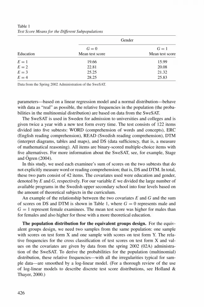
Table 1Test Score Means for the Different Subpopulations

Gender

G = 0 G = 1Education Mean test score Mean test score

E = 1 19.66 15.99E = 2 22.81 20.08E = 3 25.25 21.32E = 4 28.25 25.83

Data from the Spring 2002 Administration of the SweSAT.

parameters—based on a linear regression model and a normal distribution—behavewith data as “real” as possible, the relative frequencies in the population (the proba-bilities in the multinomial distribution) are based on data from the SweSAT.

The SweSAT is used in Sweden for admission to universities and colleges and isgiven twice a year with a new test form every time. The test consists of 122 itemsdivided into five subtests: WORD (comprehension of words and concepts), ERC(English reading comprehension), READ (Swedish reading comprehension), DTM(interpret diagrams, tables and maps), and DS (data sufficiency, that is, a measureof mathematical reasoning). All items are binary-scored multiple-choice items withfive alternatives. For more information about the SweSAT, see, for example, Stageand Ogren (2004).

In this study, we used each examinee’s sum of scores on the two subtests that donot explicitly measure word or reading comprehension; that is, DS and DTM. In total,these two parts consist of 42 items. The covariates used were education and gender,denoted by E and G, respectively. For our variable E we divided the large number ofavailable programs in the Swedish upper secondary school into four levels based onthe amount of theoretical subjects in the curriculum.

An example of the relationship between the two covariates E and G and the sumof scores on DS and DTM is shown in Table 1, where G = 0 represents male andG = 1 represent female examinees. The mean test score was higher for males thanfor females and also higher for those with a more theoretical education.

The population distribution for the equivalent groups design. For the equiv-alent groups design, we need two samples from the same population: one samplewith scores on test form X and one sample with scores on test form Y. The rela-tive frequencies for the cross classification of test scores on test form X and val-ues on the covariates are given by data from the spring 2002 (02A) administra-tion of the SweSAT. To derive the probabilities for the population (multinomial)distribution, these relative frequencies—with all the irregularities typical for sam-ple data—are smoothed by a log-linear model. (For a thorough review of the useof log-linear models to describe discrete test score distributions, see Holland &Thayer, 2000.)

426

Linear Equating with Covariates

The logarithm of the probability p jkl , for the combination of score X = x j (forj = 1, . . . , 43), gender G = k(for k = 0, 1), and education E = l (for l = 1, . . . , 4),is defined as

log(pjkl) = α + γG G +3∑

i=1

γEi Ei +

TX∑i=1

γXi xi

j +3∑

i=1

γGEi GEi

+TX∑i=1

γGXi Gxi

j +3∑

i=1

TX∑i ′=1

γEXii′ Ei x

i ′j ,

(32)

where

Ei ={

1 if i = l

0 if i �= l

are indicator variables used to separate the different levels of education. Note thatwith number right scores, x j is equal to j − 1. A polynomial of degree TX = 6, thatis, fitting the first six moments of the marginal distribution of X to the data, gives avery good fit.

For the multinomial distribution (describing the cross classification of scores ontest form Y and values on the covariates), we use the same model with the exceptionthat the scores on test form X were transformed into scores on test form Y using the(known) equating function.

The population distributions for the nonequivalent groups designs. For thenonequivalent groups with an anchor test design, we had to produce an anchortest because there is no anchor test in the SweSAT. To get a reasonable anchortest, we used a sample of examinees with scores from two test administrations,the 08B (fall) administration and the 09A (spring) administration. These two testforms are designed to measure the same latent trait(s). One of the test forms, the08B administration, was considered to be the regular test and a sample of 20 itemson the other test form, the 09A administration, was used as an external anchor.The length of the anchor test is 20 items, because empirical studies with exter-nal anchor tests have pointed in the direction of 20–60 items (von Davier, Hol-land, & Thayer, 2004; Kolen & Brennan, 2004; Petersen, Marco, & Stewart, 1982).Fitzpatrick (2008) also warns explicitly against using anchor tests smaller than 15items. The anchor test will be denoted test form A, and a randomly selected ex-aminee’s score on test form A is considered to be an observation on the randomvariable A.

As in the equivalent groups design, a multinomial distribution is used as the pop-ulation distribution. The probabilities are given by the relative frequencies from theSweSAT data smoothed by a log-linear model. For the first population, Population

427

Branberg and Wiberg

P, the following log-linear model is fitted to the data:

log(pjklm) = α + γG G +3∑

i=1

γEi Ei +

TX∑i=1

γXi xi

j +TA∑i=1

γAi ai

m +3∑

i=1

γGEi GEi

+TX∑i=1

γGXi Gx j

i +TA∑i=1

γGAi Gai

m +3∑

i=1

TX∑i ′=1

γEXii′ Ei x

i ′j

+3∑

i=1

TA∑i ′=1

γEAii ′ Ei a

i ′j +

IA∑i=1

IX∑i ′=1

γAXii ′ ai

m xi ′j +

3∑i=1

TX∑i ′=1

γGEXii′ GEi x

i ′j

+3∑

i=1

TA∑i ′=1

γGEAii′ GEi a

i ′j , (33)

where am , for m = 1, . . . , 21, is an observation on A. With number right scores, am

is equal to m − 1. For the data used in this application we settle on a model withTX = 5, TA = 5, IX = 2, and IA = 2. TX and TA are the polynomial degrees and thenumber of moments fitted to the marginal distributions of X and A, respectively. IX

and IA define the number and type of cross moments fitted to the joint distributionof X and A. In summary, we fit the log-linear model in Equation 33 to the SweSATdata and used this estimated model to calculate the probabilities in the multinomialdistribution describing the distribution of scores and covariates in Population P. Withthis population model, the means for the different subpopulations are the ones pre-sented in Table 2. As we can see, the highest mean value was in the subpopulationwith E = 4 and G = 0 and the lowest mean value was in the subpopulation withE = 1 and G = 1. The correlation between X and A(not presented in the table)was .78.

For the second population, Population Q, we used the same model but with theprobabilities adjusted as if the number of examinees with G = 0 and E = 3 weretripled and the number of examinees with G = 0 and E = 4 were doubled. Be-cause of this change, the overall ability is higher in Population Q than in Popula-tion P. However, note that the conditional distribution within each subpopulation isunchanged. The subpopulation means presented in Table 2 are the same in both pop-ulations. As in the equivalent groups design, we can use the equating function toobtain the scores on test form Y from the scores on test form X.

For the nonequivalent groups design without any anchor test, we used the samepopulations, but we did not use scores on the anchor test in the equating process.

The Simulations

In both the equivalent groups design and the nonequivalent groups designs, twoindependent samples were generated. Generating observations from a multinomialdistribution is easily done using a computer and a suitable computer program.

With the equivalent groups design we needed two samples from the same pop-ulation. The first sample was generated using a multinomial distribution with the

428

Table 2Means on the Regular Test (X) and the Anchor Test (A) in Different Subpopulations

G = 0 G = 1

Mean X Mean A Mean X Mean A

E = 1 20.354 10.063 18.066 8.283E = 2 21.914 10.677 19.714 9.064E = 3 23.459 11.629 21.351 10.094E = 4 26.349 13.012 24.974 11.758

probabilities given by the log-linear model in Equation 32 fitted to the SweSAT data.For each observation we get a score on test form X and values on the covariates.The second sample was generated from exactly the same distribution with the ex-ception that the variable Y = 2 + X was used instead of X. That is, the parametersof the equating function in the population were set to b0 = 2 and b1 = 1. Knowingthe true values of the parameters is essential if we want to evaluate the efficiency ofthe estimators. Finally, the two samples were used to estimate the equating param-eters using the model and the method described earlier. This procedure was repli-cated 20,000 times, giving us estimates of the sampling distributions. The samplesizes used for the different simulations are nX = nY = 2000, nX = nY = 500, andnX = nY = 200.

The procedure was almost the same when we have the nonequivalent groups de-signs. For the first sample we used a multinomial distribution with the probabilitiesgiven by the log-linear model in Equation 33 fitted to the SweSAT data. For thesecond sample we used the variable Y = 2 + X instead of X. However, with thenonequivalent groups design, we also changed the probabilities in the multinomialdistribution. As described earlier, the probability of getting an observation from thesubpopulation with G = 0 and E = 3 or the subpopulation with G = 0 and E = 4is increased. The effect is that the second sample was generated from a populationhaving a higher overall ability. The number of replications and the sample sizes werethe same as in the equivalent groups design.

Finally, for comparison purposes an equating using the Tucker method (which hassimilar assumptions as the proposed method) was added in the nonequivalent groupswith an anchor test design. A brief description of the Tucker method follows below;for a detailed description, see Kolen & Brennan (2004). The Tucker method is basedon two assumptions: (a) the regressions of X and Y on the anchor scoreA are thesame linear functions in both populations, and (b) the conditional variances of Xand Y given A are the same for both populations (Braun & Holland, 1982; Kolen& Brennan, 2004; von Davier & Kong, 2005). The Tucker method assumes a syn-thetic population S = w1 P + (1 − w2)Q, which is a weighted combination of twopopulations P and Q that take X and Y, respectively. The weights w1 and w2 satisfythe constraint w1 + w2 = 1 (Braun & Holland, 1982, sect. 3.3.2). In our examplesthe samples were given the same weights (w = w1 = w2 = 0.5) because the popula-tions were considered to be equally important (Kolen & Brennan, 2004, sect. 4.1.5).

429

Branberg and Wiberg

Using the above assumptions, the means and standard deviations in Equation 5 canbe derived as

μS(X ) = μP (X ) − wQλP (μP (A) − μQ(A)), (34)

μS(Y ) = μQ(Y ) − wPλQ(μP (A) − μQ(A)), (35)

σ2S(X ) = σ2

P (X ) − wQλ2P

(σ2

P (A) − σ2Q(A)

) + wPwQλ2P (μP (A) − μQ(A))2, (36)

σ2S(Y ) = σ2

Q(Y ) − wPλ2Q

(σ2

P (A) − σ2Q(A)

) + wPwQλ2Q(μP (A) − μQ(A))2, (37)

with λP and λQ as regression slopes defined by λP = σ2P (X , A)/σ2

P (A) and λQ =σ2

Q(Y, A)/σ2Q(A). Plugging the sample equivalents of these parameters into Equation

5, an estimate of the Tucker linear equating transformation is obtained.

Results

Several models with different combinations of covariates and (in the nonequiva-lent groups with an anchor test design) scores on an anchor test were compared. Forall equating with covariates and/or anchor scores, the estimators presented in Equa-tions 24–27 were used except when we used the Tucker method. Some of the moreinteresting results are summarized below. For the reader interested in details, moreresults are available from the authors.

The Equivalent Groups Design

In Table 3, the results from the estimation of b0 and b1 are summarized. The valuespresented in the table are the mean, standard deviation, and MSE for each estimatedsampling distribution, that is, each value in the table is based on 20,000 observa-tions. As we can see, there was almost no bias no matter which model we used. Theestimated expected value of b1 was (rounded to two decimal places) 1.00, which isthe true value of b1, and the estimated expected value of was equal to the true value2.00 or very close to that value. In our view, the tendency for b0 to underestimate b0,especially in small samples, is not large enough to be of any great concern. The de-viation from the true value was in some cases statistically significant (using ordinaryt-tests), but we do not think that it is practically significant.

The standard deviation can obviously be reduced by using covariates. With bothE and G in the model, the standard deviation of b0 was reduced 7.3% (from .495 to.459) when the sample sizes were nX = nY = 2000 and 8.0% when the sample sizeswere nX = nY = 200. The corresponding figures for b1 are 4.7% and 6.0%. We alsocan see that there is no point in adding an interaction between G and E to the model.The standard deviations and the MSE were almost the same as for the model withoutthe interaction.

430

Table 3Estimated Expected Values, μ, Standard Deviations, σ, and Mean Squared Errors ( M SE) ofthe Estimators b0 and b1 for Different Models and Different Samples Sizes in the EquivalentGroups Design

Model Sample Sizes μ(b0) σ(b0) M SE(b0) μ(b1) σ(b1) M SE(b1)

No covariates 2000 1.99 .495 .245 1.00 .0192 .000368500 2.00 .997 .993 1.00 .0389 .001511200 1.96 1.595 2.545 1.00 .0620 .003843

G 2000 1.99 .488 .238 1.00 .0191 .000363500 1.99 .973 .947 1.00 .0380 .001447200 1.96 1.551 2.408 1.00 .0605 .003659

E 2000 1.99 .463 .215 1.00 .0185 .000343500 1.98 .929 .864 1.00 .0371 .001379200 1.94 1.487 2.216 1.00 .0592 .003512

G + E 2000 2.00 .459 .211 1.00 .0183 .000334500 2.00 .924 .853 1.00 .0368 .001354200 1.95 1.467 2.153 1.00 .0583 .003401

G+ E+ G∗E 2000 2.00 .457 .209 1.00 .0183 .000336500 1.98 .922 .851 1.00 .0369 .001363200 1.97 1.457 2.124 1.00 .0582 .003394

In an equating, the most interesting estimators are the estimators of the equatedvalues. In Figure 1, we can see that the MSE for these estimators was reduced whencovariates were used. For every value on X, the two curves showing the MSE forthe models with covariates are below the curve showing the MSE for the modelwithout covariates. In terms of low MSE, the models with covariates were betterthan the model without covariates. In Figure 1, the sample sizes are nX = nY = 500but we obtained the same pattern when the sample sizes were nX = nY = 2000 ornX = nY = 200. Some of these results (for x = 10, x = 20, and x = 30) are pre-sented in Table 4. This table also includes estimated expected values and estimatedstandard deviations. Note that when the sample sizes are nX = nY = 2000 the stan-dard deviation of eY (20) is reduced more than 13% (from .716 to .627) when bothcovariates (without interaction) are used; the MSE is reduced 24.8% (from .0516 to.0388).

In summary, this simulation study indicated that, with an equivalent groups design,the accuracy of the estimators can be improved by using covariates (background vari-ables correlated with the test score). Although the two samples in the study are statis-tically equivalent (they are random samples from the same population), the MSE ofthe estimator of the equated value when x = 20 is reduced almost 25% when genderand education are used as covariates.

The Nonequivalent Groups Designs

In a nonequivalent groups design, the two groups can be nonequivalent in manydifferent ways. In this study, the difference between the two populations is in the

431

Table 4Estimated Expected Values, μ, Standard Deviations, σ, and Mean Squared Errors ( M SE), ofthe Estimators eY (10), eY (20) and eY (30) for Different Models with the Equivalent GroupsDesign

Sample Sizes

200 2000

Model x μ(eY (x)) σ(eY (x)) M SE(eY (x)) μ(eY (x)) σ(eY (x)) M SE(eY (x))

No covariates 10 11.98 1.070 1.145 12.00 .334 .111320 21.99 .716 .513 22.00 .227 .051630 32.01 .806 .650 32.00 .256 .0655

G 10 11.98 1.038 1.078 12.00 .327 .106920 21.99 .692 .479 22.00 .220 .048330 32.01 .782 .612 32.00 .250 .0623

E 10 11.96 .981 .964 11.99 .306 .093420 21.99 .644 .415 22.00 .202 .040730 32.01 .754 .569 32.00 .238 .0567

G + E 10 11.97 .966 .933 12.00 .302 .091320 21.99 .627 .393 22.00 .197 .038830 32.01 .731 .534 32.00 .231 .0532

G + E + 10 11.98 .960 .921 12.00 .300 .0903G∗E 20 22.00 .630 .398 22.00 .196 .0385

30 32.01 .743 .552 32.00 .232 .0538

distribution on the covariates G and E, making the overall ability higher in one ofthe populations (Population Q). In Table 5, some of the results from the estimationof the equating parameters b0 and b1 are shown. When there are no covariates andno anchor test in the model, the estimator used to estimate b0 has a considerablebias. The reason for the bias is that the overall ability is higher in the group takingthe harder test. This difference between the groups disguises some of the differencein difficulty between the test forms. The bias was smaller when we used one ofthe covariates. It became even smaller when we use an anchor test, and it almostdisappeared when we used both G and E, the two variables causing the differencebetween the groups.

The MSE is much smaller when we used models with an anchor test; it was re-duced even further when we used a covariate. With E added to a model with ananchor test, M SE(b0) was reduced 8.7% (from .150 to .137) when the sample sizeswere nX = nY = 2000 and 4.6% when the sample sizes were nX = nY = 500. Whenestimating b1, the pattern was the same but the difference between a model with onlyan anchor test and a model with an anchor test and covariates was smaller. Note,however, that in the absence of an anchor test, a model with the two covariates Gand E gives a rather accurate estimation of the parameters in the equating function,especially when the sample sizes are nX = nY = 2000. An interesting result is thatthe maximum likelihood estimators (MLE), derived using the (false) assumption ofnormality, were slightly more efficient than were the Tucker estimators.

432

Figure 1. The mean squared error (MSE) of eY (x) for three differentmodels with the equivalent groups design and sample sizesnX = nY = 500.

Some of the results from the estimation of the equated values are shown in Figure 2and Table 6. With sample sizes nX = nY = 500, the best model in terms of low MSEwas the model with an anchor test plus E as an additional covariate. However, as wecan see in Figure 2, the difference between this best model and a model with only ananchor test was very small. The results were almost the same when the sample sizesare nX = nY = 2000 (Table 6). With very small sample sizes (nX = nY = 200), theMSE was smallest when we used both E and G together with an anchor test but theimprovement we got by adding G to the model was small.

In small samples (nX = nY = 200 or nX = nY = 500), and with a model wherewe used anchor test scores but no covariates, MLE was better than Tucker estimation(Figure 2 and Table 6). Both estimators have a small bias, but the standard deviationand MSE were smaller for MLE. With a larger sample (nX = nY = 2000), the Tuckermethod performed better when x = 10 and MLE was better when x = 30. However,the differences between the two methods were rather small.

One important result is that, in the absence of an anchor test and with samples aslarge as nX = nY = 2000, the estimation of equated values was quite accurate andwithout bias with only the two covariates G and E in the model.

In summary, the results of this simulation study indicate that with a nonequivalentgroups design the most efficient way to estimate the equating parameters is to usea good anchor test. The accuracy of the estimators can (at least in some cases) be

433

Table 5Estimated Expected Values, μ, Standard Deviations, σ, and Mean Squared Errors ( M SE) ofthe Estimators b0 and b1 for Different Models and Different Samples Sizes with theNonequivalent Groups Design

Model Sample Size μ(b0) σ(b0) M SE(b0) μ(b1) σ(b1) M SE(b1)

No covariates 2000 1.49 .465 .474 1.00 .0193 .000385500 1.49 .937 1.140 1.00 .0388 .001510200 1.46 1.485 2.493 1.00 .0618 .003816

A, Tucker 2000 1.95 .390 .155 1.00 .0172 .000299500 1.94 .787 .623 1.00 .0347 .001203200 1.92 1.251 1.572 1.00 .0552 .003047

A, MLE 2000 1.92 .379 .150 1.00 .0164 .000269500 1.91 .761 .588 1.00 .0329 .001083200 1.88 1.203 1.461 1.00 .0523 .002733

G 2000 1.71 .463 .301 1.00 .0193 .000375500 1.69 .919 .938 1.00 .0383 .001474200 1.66 1.469 2.276 1.00 .0614 .003783

E 2000 1.81 .446 .234 1.00 .0189 .000362500 1.80 .892 .838 1.00 .0378 .001432200 1.79 1.436 2.105 1.00 .0606 .003668

A + G 2000 1.93 .378 .149 1.00 .0164 .000270500 1.91 .763 .590 1.00 .0333 .001110200 1.90 1.199 1.448 1.00 .0521 .002713

A + E 2000 2.00 .375 .137 1.00 .0163 .000266500 1.98 .749 .561 1.00 .0327 .001073200 1.97 1.203 1.448 1.00 .0524 .002745

G + E 2000 1.98 .445 .199 1.00 .0188 .000357500 1.97 .888 .789 1.00 .0380 .001449200 1.95 1.416 2.009 1.00 .0602 .003634

A + G + E 2000 2.00 .376 .141 1.00 .0164 .000270500 1.99 .758 .575 1.00 .0331 .001093200 1.97 1.198 1.00 .0520 .002709

improved by supplementing anchor test scores with observations on covariates, butthe improvement is small. In the absence of an anchor test, the equating can be im-proved if covariates are used to correct for differences between the groups, providedthat we can find covariates that can “explain” these differences. This is of particu-lar interest for testing programs, like the SweSAT, where legislative, administrative,and/or economic restrictions make it difficult to use an anchor test.

Numerical Illustration

To illustrate the use of the model and the techniques presented earlier with realdata, we equated two administrations, 87A (spring) and 87B (fall), of the SweSAT.In the sequel, the variables Y and X are the raw scores on 87A and 87B, respectively.The 1987 SweSAT consisted of six subtests covering the areas of vocabulary, data

434

Table 6Estimated Expected Values, μ, Standard Deviations, σ, and Mean Squared Errors ( M SE) ofthe Estimators eY (10), eY (20), and eY (30) for Different Models with the NonequivalentGroups Design

Sample sizes

200 2000

Model x μ(eY (x)) σ(eY (x)) M SE(eY (x)) μ(eY (x)) σ(eY (x)) M SE(eY (x))

No covariates 10 11.45 .976 1.249 11.46 .307 .386220 21.43 .682 .792 21.43 .215 .375130 31.41 .860 1.087 31.39 .271 .4378

A, Tucker 10 11.92 .763 .589 11.93 .238 .060620 21.91 .456 .215 21.91 .143 .027930 31.91 .666 .451 31.90 .209 .0540

A, MLE 10 11.90 .744 .564 11.92 .235 .062220 21.91 .455 .214 21.91 .144 .028030 31.93 .637 .411 31.91 .200 .0475

G 10 11.69 .966 1.029 11.72 .305 .171620 21.72 .680 .514 21.73 .213 .116830 31.75 .863 .805 31.75 .270 .1370

E 10 11.78 .934 .919 11.79 .290 .127320 21.77 .644 .467 21.77 .201 .092730 31.76 .831 .748 31.75 .261 .1305

A + G 10 11.92 .744 .561 11.93 .235 .060820 21.93 .459 .216 21.93 .146 .026930 31.94 .641 .414 31.93 .203 .0470

A + E 10 11.98 .744 .553 12.00 .232 .053020 22.00 .456 .208 22.00 .143 .020430 32.01 .641 .411 32.00 .200 .0402

G + E 10 11.98 .920 .847 12.00 .291 .084820 22.01 .641 .411 22.02 .204 .042030 32.05 .837 .703 32.04 .264 .0708

G + E + G∗E 10 11.97 .937 .880 12.00 .288 .082720 21.99 .655 .428 22.00 .202 .040730 32.02 .854 .729 32.01 .262 .0685

A + G + E 10 11.98 .742 .552 12.00 .232 .054020 21.99 .456 .208 22.00 .143 .020630 32.01 .638 .407 32.01 .203 .0413

sufficiency, reading comprehension, interpretation of diagrams, tables and maps, so-cial science/general information, and study technique. In total, the test consists of atotal of 144 multiple choice items. For more details about these older versions of theSweSAT, see Henrysson and Wedman (1975).

The SweSAT is given twice a year, with a new test form every time. Because thetest result can be used for several years after the test administration date, resultsfrom different administrations are compared in the selection process and there is

435

Figure 2. Mean squared error (MSE) of eY (x)for six different modelswith the nonequivalent groups design and sample sizes nX = nY = 500.

therefore a need to equate test scores from different test forms. However, none of therequirements for standard equating are fulfilled. There is no anchor test (all itemsare released after the administration of the test), and there may be systematic differ-ences in ability between the examinee groups, which makes an assumption of ran-dom samples from the same population implausible. To adjust for these differences,an important part of the equating process is matching of samples on covariates. (Formore details about the SweSAT and the equating of the SweSAT, see Emons, 1998;Lyren & Hambleton, 2008; and Stage & Ogren, 2004).

Because the SweSAT is designed to measure more than one dimension, it can beargued that the equating should be done on a subtest level. An assumption of differenttest forms measuring the same ability is probably more seriously violated on a totalscore level. On the other hand, the equating actually performed was done on a totalscore level and we will follow that principle in this illustration to make comparisonspossible. The background variables used were gender (G), education (E), and age(Ag). The number of examinees taking the 87A administration was nY = 5923, andthe number of examinees taking the 87B administration was nX = 3666.

Table 7 presents estimates of the equating parameters for different combinationsof covariates together with equated scores using the parameter estimates. In the table,raw scores on 87B were transformed to the 87A scale. The estimates in the first roware given by b1 = s−1

X sY and b0 = y − s−1X sY x, that is, a standard observed score

linear equating using the assumption of random samples from the same population.The estimates in the other rows are given by the estimators in Equations 24–27.

436

Table 7Estimates of the Equating Parameters for Different Models and Equated Scores for SomeSelected Raw Scores on Test Form 87B

Equating Parameters Raw Scores

Covariates in the model b0 b1 50 80 100 130

No covariates 2.91 .995 52.65 82.49 102.38 132.22G 2.88 .994 52.58 82.39 102.27 132.09Ag 2.15 .998 52.06 82.01 101.97 131.92E .77 1.008 51.16 81.39 101.55 131.78G + Ag 2.30 .995 52.03 81.87 101.76 131.60G + E 1.02 1.004 51.22 81.33 101.41 131.53Ag + E .58 1.007 50.95 81.16 101.31 131.53G + Ag + E .73 1.004 50.92 81.03 101.10 131.21

The results in Table 7 indicate that the 87B administration was somewhat moredifficult than the 87A administration. If we ignore differences in distribution on co-variates and act as if the examinee groups are random samples from the same pop-ulation, we would say that the difference between the two administrations is about2–3 points. On the other hand, the equating using all three covariates suggests a dif-ference of about 1 point. According to this latter method, much of the difference seenin the equating with no covariates is not a result of differences between the two testforms but can be “explained” by differences between the two examinee groups inthe distribution on gender, education, and age. If we compare the results from themodels with covariates with the result from the equating with no covariates, we seethat the largest adjustments occurred when E was one of the variables in the model.The explanation is that there is a considerable difference between the two examineegroups in the distribution on education. The proportion of well-educated examineeswas much higher in the group taking test form 87A.

A problem with real data is that we do not know the “true” equating function.However, we do know the estimates that actually were used when the two tests wereequated. These were b0 = 1 and b1 = 1 and therefore were rather close to the resultswe got with our method. This is not a strong argument in support of the method used,but it is an indication that (at least in this case) the estimates are reasonable.

Discussion

The model presented in this paper consists of two parts. First, we have a linearregression part connecting the covariates with the observed scores. Second, we havea linear equating part connecting observed scores on the two test forms with eachother. To relax these linearity assumptions may be an area for future research. Oneinteresting possibility is to investigate the effect of using covariates with an equiper-centile equating function.

To estimate the parameters of the model, we assume a normal distribution anduse maximum likelihood estimation. In our simulation study this works rather well,

437

Branberg and Wiberg

even though the data are generated from a multinomial distribution. To maximize alikelihood function based on normality is only one way of estimating the parameters.One can think of both other distributions and other estimation methods.

One problem with regression-type models is finding relevant variables. Relevantvariables are, in our case, variables correlated with the test scores or, in the nonequiv-alent groups design, variables “explaining” the systematic differences between theexaminee groups. Missing important explanatory variables in a nonequivalent groupsdesign may result in biased estimators; it is the same as treating the samples as sta-tistically equivalent when they are, in fact, nonequivalent. The importance of theproblem will depend on the size of the bias. To investigate the robustness of the esti-mators when important explanatory variables are missing can be an area for furtherresearch.

In the SweSAT, the test forms are administered at different points in time; the as-sumption of equal regression relationships in both populations therefore is equivalentto an assumption of equal regression relationships over time. A violation of this as-sumption usually can be seen as a misspecification of the model. There is a changeover time unexplained by the variables included in the model. If such a change isslow, the assumption of equal regression relationships may be reasonable and thebias small if the time interval between the administrations of the test forms is not toolong.

The evidence from the simulation study in this paper indicates that the accuracyof an equating can be increased by using covariates in the equating process. Withthe equivalent groups design, all the models with covariates were better (in termsof lower MSE) than the model without covariates. We used gender and educationas covariates, a choice more or less determined by the availability of data. With abetter choice of variables based on strong theory and empirical research, it may bepossible to increase the efficiency of the estimators even more. One possibility worthconsidering in future research is to use many variables summarized in a propensityscore, as suggested by Livingston et al. (1990).

In the nonequivalent groups design, using an anchor test is the best method toadjust for the systematic differences between the groups. The results in this paperindicate that the estimation can be (marginally) improved by supplementing the an-chor test with other variables correlated with the test score. In theory, the anchor testA is measuring exactly the same thing as the test forms X and Y. With this in mind,one would expect the anchor test to explain all the differences between the groupsand thus make the use of covariates redundant. However, not all tests are exactlyone-dimensional and not all anchor tests are measuring exactly the same construct(s)as the test forms X and Y. There may be some variation in the test scores not ex-plained by the anchor test. If this is the case, covariates may be used to reduce theMSE of the estimators. It also is possible that covariates can play a role if the anchortest A is short as compared to the test forms X and Y. In this case, one can expectsome systematic variation not explained by the anchor test. As an extreme exampleto illustrate the point, suppose that the anchor test consists of only one item. Eachexaminee will have a score of 0 or 1 on the anchor test. Conditional on the score onthe anchor test, say the group with a score of 0, there will probably be a variation inthe scores on test form X and test form Y that will depend on background variables

438

Linear Equating with Covariates

such as education, gender, and so on. In this case, covariates can be used to reducethe MSE of the estimators.

In the nonequivalent groups design with no anchor test (as in the SweSAT), thecovariates can be used to adjust for the systematic differences between the groups.This is usually not as efficient as the use of an anchor test, but our simulations showthat with the right covariates (i.e., covariates explaining the systematic differencesbetween the groups) the bias can be eliminated. The precision of the estimators alsowas quite good. In the numerical illustration we also showed that the results froman equating of two administrations of the SweSAT were close to the results from theequating actually performed. The overall result, that we can increase the accuracy inthe equating by using covariates when we have nonequivalent groups design with noanchor test, is important since there are several standardized tests (e.g., the SweSAT)that do not have an anchor test.

References

Angoff, W. H. (1971). Scales, norms, and equivalent scores. In R. L. Thorndike (Ed.), Ed-ucational measurement (2nd ed.) (pp. 508–600). Washington, DC: American Council onEducation (Reprinted by Educational Testing Service, Princeton NJ, 1984).

Braun, H. I., & Holland, P. W. (1982). Observed-score test equating: A mathematical analysisof some ETS equating procedures. In P. W. Holland & D. B. Rubin (Eds.), Test equating(pp. 9–49). New York, NY: Academic Press.

Branberg, K. (1997). On test score equating (Statistical Studies No 23). Umea, Sweden: De-partment of Statistics, Umea University.

Branberg, K., Henriksson, W., Nyquist, H., & Wedman, I. (1990). The influence of sex, educa-tion and age on the scores on the Swedish Scholastic Aptitude Test. Scandinavian Journalof Educational Research, 34, 189–203.

Cook, L. L., Eignor, D. R., & Schmitt, A. P. (1990). Equating achievement tests using sam-ples matched on ability (College Board Report 90–2). New York, NY: College EntranceExamination Board.

Dorans, N. J. (Ed.) (2004). Assessing the population sensitivity of equating functions [Specialissue]. Journal of Educational Measurement, 41(1).

Dorans, N. J., Liu, J., & Hammond, S. (2008). Anchor test type and population invariance: Anexploration across subpopulations and test administrations. Applied Psychological Mea-surement, 32(1), 81–97.

Emons, W. H. M. (1998). Nonequivalent groups IRT observed score equating. Its applicabilityand appropriateness for the Swedish Scholastic Aptitude Test (EM No 32). Umea, Sweden:Department of Educational Measurement, Umea University.

Fitzpatrick, A. R. (2008). The impact of anchor-test configuration on student proficiency rates.Educational Measurement: Issues and Practice, 27(4), 34–40.

Henrysson, S., & Wedman, I. (1975). The contents of the Scholastic Aptitude Test (Spanor franSpint, No. 3). Umea, Sweden: Department of Education, Umea University.

Holland, P. W., Dorans, N. J., & Petersen, N. S. (2007). Equating test scores. In C. R. Rao & S.Sinharay (Eds.), Handbook of statistics (Vol. 26, pp. 169–203). Oxford, England: Elsevier.

Holland, P. W., & Thayer, D. T. (2000). Univariate and bivariate loglinear models for dis-crete test score distributions. Journal of Educational and Behavioral Statistics 25(2),133–183.

Kolen, M. J. (1990). Does matching in equating work? A discussion. Applied Measurement inEducation, 3(1), 23–39.

439

Branberg and Wiberg

Kolen, M. J., & Brennan, R. L. (2004). Test equating, scaling and linking: Methods and prac-tices (2nd ed.). New York, NY: Springer.

Liou, M., Cheng, P. E., & Li, M. (2001). Estimating comparable scores using surrogate vari-ables. Applied Psychological Measurement, 25(2), 197–207.

Liu, M., & Holland, P. W. (2008). Exploring population sensitivity of linking functionsacross three law school admission test administrations. Applied Psychological Measure-ment, 32(1), 27–44.

Livingston, S. A., Dorans, N. J., & Wright, N. K. (1990). What combination of sampling andequating methods works best? Applied Measurement in Education, 3(1), 73–95.

Lyren, P.-E., & Hambleton, R. K. (2008). Systematic equating error with the randomly-equivalent groups design: An examination of the equal ability distribution assumption (EMNo 61). Umea, Sweden: Department of Educational Measurement, Umea University.

Petersen, N. S., Marco, N. S., & Stewart, E. E. (1982). A test of adequacy of linear scoreequating models. In P. W. Holland & D. B. Rubin (Eds.), Test equating (pp. 71–135). NewYork, NY: Academic Press.

Potthoff, R. F. (1966). Equating of grades or scores on the basis of a common battery ofmeasurements. In P. R. Krishnaiah (Ed.), Multivariate Analysis: Proceedings of an Interna-tional Symposium held in Dayton, Ohio, June 14–19, 1965 (pp. 541–559). New York, NY:Academic Press.

Stage, C., & Ogren, G. (2004). The Swedish Scholastic Assessment Test (SweSAT). Develop-ment, results and experiences (EM No. 49). Umea, Sweden: Department of EducationalMeasurement, Umea University.

von Davier, A. A., Holland, P. W., & Thayer, D. T. (2004). The kernel method of test equating.New York, NY: Springer.

von Davier, A. A., & Kong, N. (2005). A unified approach to linear equating for the nonequiv-alent groups design. Journal of Educational and Behavioral Statistics, 30, 313–342.

Wright, N. K., & Dorans, N. J. (1993). Using the selection variable for matching or equating(Research Report RR-93–04). Princeton, NJ: Educational Testing Service.

Yang, W.-L., & Gao, R. (2008). Invariance of score linkings across gender groups for formsof a testlet-based college level examination program examination. Applied PsychologicalMeasurement, 32(1), 45–61.

Yi, Q., Harris, D. J., & Gao, X. (2008). Invariance of equating functions across different sub-groups of examinees taking a science achievement test. Applied Psychological Measure-ment, 32(1), 62–80.

Authors

KENNY BRANBERG is a Researcher at the Department of Statistics, Umea University, SE-90187 Umea, Sweden; kenny.branberg@stat.umu.se. His primary research interests includepsychometrics and test equating.

MARIE WIBERG is an Associate Professor, Department of Statistics, Umea University, SE-90187 Umea, Sweden; marie.wiberg@stat.umu.se. Her primary research interests includepsychometrics, test equating, applied statistics, and international large-scale assessments.

440