Of Mice and Models

Marco Ajmone Marsan, Giovanna Carofiglio, Michele Garetto, Paolo Giaccone,Emilio Leonardi, Enrico Schiattarella, and Alessandro Tarello

Dipartimento di Elettronica, Politecnico di Torino, C.so Duca degli Abruzzi 24, Torino, Italy�

firstname.lastname@polito.it

Abstract. Modeling mice in an effective and scalable manner is one of the mainchallenges in the performance evaluation of IP networks. Mice is the name thathas become customary to identify short-lived TCP connections, that form the vastmajority of packet flows over the Internet. On the contrary, long-lived TCP flows,that are far less numerous, but comprise many more packets, are often calledelephants. Fluid models were recently proved to be a promising effective andscalable approach to investigate the dynamics of IP networks loaded by elephants.In this paper we extend fluid models in such a way that IP networks loaded bytraffic mixes comprising both mice and elephants can be studied. We then showthat the newly proposed class of fluid models is quite effective in the analysis ofnetworks loaded by mice only, since this traffic is much more critical than a mixof mice and elephants.

1 Introduction

The traffic on the Internet can be described either at the packet level, modeling thedynamics of the packet generation and transmission processes, or at the flow level,modeling the start times and durations of sequences of packet transfers that correspondto (portions of) a service requested by an end-user. Examples of flows can be either thetrain of packets corresponding to an Internet telephone call, or the one correspondingto the download of a web page. In the latter case, the flow can be mapped onto a TCPconnection. This is the most common case today in the Internet, accounting for thevast majority of traffic. The number of packets in TCP connections is known to exhibita heavy-tailed distribution, with a large number of very small instances (called TCPmice) and few very large ones (called elephants).

Models for the performance analysis of the Internet have been traditionally based ona packet-level approach for the description of Internet traffic and of queuing dynamicsat router buffers. Packet-level models allow a very precise description of the Internetoperations, but suffer severe scalability problems, such that only small portions of realnetworks can be studied.

Fluid models have been recently proposed as a scalable approach to describe thebehavior of the Internet. Scalability is achieved by describing the network and trafficdynamics at a higher level of abstraction with respect to traditional discrete packet-level models. This implies that the short-term random effects typical of the packet-levelnetwork behavior are neglected, focusing instead on the longer-term deterministic flow-level traffic dynamics.

� This work was supported by the Italian Ministry for Education, University and Research,through the FIRB project TANGO.

M. Ajmone Marsan et al. (Eds.): QoS-IP 2005, LNCS 3375, pp. 15–32, 2005.c© Springer-Verlag Berlin Heidelberg 2005

16 Marco Ajmone Marsan et al.

In fluid flow models, during their activity period, traffic sources emit a continu-ous information stream, the fluid flow, which is transferred through a network of fluidqueues toward its destination (also called sink).

The dynamics of a fluid model, which are continuous in both space and time, arenaturally described by a set of ordinary differential equations, because of their intrinsicdeterministic nature.

Fluid models were first proposed in [1–4] to study the interaction between TCP ele-phants and a RED buffer in a packet network consisting of just one bottleneck link, ei-ther ignoring TCP mice [1–3], or modeling them as unresponsive flows [4] introducinga stochastic disturbance. In this case, fluid models offer a viable alternative to packet-based simulators, since their complexity (i.e., the number of differential equations tobe solved) is independent of both the number of TCP flows and the link capacity. InSection 2 we briefly summarize the fluid models proposed in [1–3], which constitutethe starting point for our work.

Structural properties of the fluid model solution were analyzed in [5], while im-portant asymptotic properties were proved in [6, 7]. In the latter works, it was shownthat fluid models correctly describe the limiting behavior of the network when both thenumber of TCP elephants and the bottleneck link capacity jointly tend to infinity.

The single bottleneck model was then extended to consider general multi-bottlenecktopologies comprising RED routers in [3, 8].

In all cases, the set of ordinary differential equations of the fluid model are solvednumerically, using standard discretization techniques.

An alternative fluid model was proposed in [9, 10] to describe the dynamics of theaverage window for TCP elephants traversing a network of drop-tail routers. The be-havior of such a network is pulsing: congestion epochs, in which some buffers areoverloaded (and overflow), are interleaved to periods of time in which no buffer isoverloaded and no loss is experienced, due to the fact that previous losses forced TCPsources to reduce their sending rate. In such a setup, a careful analysis of the averageTCP window dynamics at congestion epochs is necessary, whereas sources can be sim-ply assumed to increase their rate at constant speed between congestion epochs. Thisbehavior allows the development of differential equations and an efficient methodologyto solve them. Ingenious queueing theory arguments are exploited to evaluate the lossprobability during congestion epochs, and to study the synchronization effect amongsources sharing the same bottleneck link. Also in this case, the complexity of the fluidmodel analysis is independent of both the link capacities and the number of TCP flows.

Extensions that allow TCP mice to be considered are outlined in [9, 10] and in [8].In this case, since the dynamics of TCP mice with different size and/or different starttimes are different, each mouse must be described with two differential equations; onerepresenting the average window evolution, and one describing the workload evolu-tion. As a consequence, one of the nicest properties of fluid models, the insensitivity ofcomplexity with respect to the number of TCP flows, is lost.

In [11] a different description of the dynamics of traffic sources is proposed, that ex-ploits partial differential equations to analyze the asymptotic behavior of a large numberof TCP elephants through a single bottleneck link fed by a RED buffer.

Of Mice and Models 17

In [12] we built on the approach in [11], showing that the partial differential equa-tion description of the source dynamics allows the natural representation of mice aswell as elephants, with no sacrifice in the scalability of the model.

The limiting case of an infinite number of TCP mice is considered in [13], whereit is proved that, even in the case of loads lower than 1, deterministic synchronizationeffects may lead to congestion and to packet losses.

When the network workload is composed of a finite number of TCP mice, normallythe link loads (given by the product of the mice arrival rate times the average micelength) are well below link capacities. In this case, the deterministic nature of fluidmodels leads to predict that buffers are always empty, and this fact contradicts the ob-servations made on real packet networks. This discrepancy is due to the fact that, inunderload conditions, the stochastic nature of the input traffic plays a fundamental rolein the network dynamics, which cannot be captured by the determinism of fluid models.

In [12] we first discussed the possibility of integrating stochastic aspects within fluidmodels. We proposed a preliminary solution to the problem, exploiting a hybrid fluid-Montecarlo approach. In [14] we further investigate the possibilities for the integrationof randomness in fluid models, proposing two additional approaches, which rely onsecond-order Gaussian approximations of the stochastic processes driving the networkbehavior.

In this paper, we consider the hybrid fluid-Montecarlo approach proposed in [12],further investigating the impact that different modeling choices can have in different dy-namic scenarios. We present numerical results to show that the hybrid fluid-Montecarloapproach is capable of producing reliable performance predictions for networks thatoperate far from saturation. In addition, we prove the accuracy and the flexibility of themodeling approach by considering both static traffic patterns, from which equilibriumbehaviors can be studied, and dynamic traffic conditions, that allow the investigation oftransient dynamics.

2 Fluid Models of IP Networks

In this section we briefly summarize the fluid model presented in [1–3] and the exten-sion presented in [12].

Consider a network comprising K router output interfaces, equipped with FIFObuffers, feeding links at rate C (the extension to non-homogeneous data rates is straight-forward). The network is fed by I classes of TCP elephants; all the elephants withinthe same class follow the same route through the network, thus experiencing the sameround-trip time (RTT), and the same average loss probability. At time t = 0 all buffersare assumed to be empty. Buffers drop packets according to their instant occupancy,as in drop tail buffers, or their average occupancy, as in RED (Random Early Detec-tion [15]) active queue management (AQM) schemes.

2.1 Elephant Evolution Equations

In [1–3], simple differential equations were developed to describe the behavior of TCPelephants over networks of IP routers adopting a RED AQM scheme. We refer to thisoriginal model with the name MGT.

18 Marco Ajmone Marsan et al.

Consider the ith class of elephants; the temporal evolution of the average windowof TCP sources in the class, Wi(t), is described by the following differential equation:

dWi(t)dt

=1

Ri(t)− Wi(t)

2λi(t) (1)

where Ri(t) is the average RTT for class i, and λi(t) is the loss indicator rate experi-enced by TCP flows of class i. The differential equation is obtained by considering thefact that elephants can be assumed to be always in congestion avoidance (CA) mode,so that the window dynamics are close to AIMD (Additive Increase, Multiplicative De-crease). The window increase rate in CA mode is linear, and corresponds to one packetper RTT. The window decrease rate is proportional to the rate with which congestion in-dications are received by the source, and each congestion indication implies a reductionof the window by a factor two.

In [12] we extended the fluid model presented in [1–3]. In our approach, that willbe named PDFM, rather than just describing the average TCP connection behavior, wetry to statistically model the dynamics of the entire population of TCP flows sharing thesame path. This approach leads to systems of partial derivatives differential equations,and produces more flexible models, which scale independently from the number of TCPflows.

To begin, consider a fixed number of TCP elephants. We use Pi(w, t) to indicatethe number of elephants of class i whose window is ≤ w at time t. For the sake ofsimplicity, we consider just one class of flows, and omit the index i from all variables.The source dynamics are described by the following equation, for w ≥ 1:

∂P (w, t)∂t

=∫ 2w

w

λ(α, t)∂P (α, t)

∂αdα − 1

R(t)∂P (w, t)

∂w(2)

where λ(w, t) is the loss indication rate. The intuitive explanation of the formula is thefollowing. The time evolution of the population described by P (w, t) is governed bytwo terms: i) the integral accounts for the growth rate of P (w, t) due to the sourceswith window between w and 2w that experience losses; ii) the second term describesthe decrease rate of P (w, t) due to sources increasing their window with rate 1/R(t).

2.2 Network Evolution Equations

In both models, Qk(t) denotes the (fluid) level of the packet queue in the kth buffer attime t; the temporal evolution of the queue level is described by:

dQk(t)dt

= Ak(t) [1 − pk(t)] − Dk(t) (3)

where Ak(t) represents the fluid arrival rate at the buffer, Dk(t) the departure rate fromthe buffer (which equals Ck, provided that Qk(t) > 0), and the function pk(t) rep-resents the instantaneous loss probability at the buffer, which depends on the packetdiscard policy at the buffer. An explicit expression for pk(t) is given in [2] for REDbuffers, while for drop-tail buffers:

pk(t) =max(0, Ak(t) − C)

Ak(t)1I{Qk(t)=Bk} (4)

Of Mice and Models 19

If Tk(t) denotes the instantaneous delay of buffer k at time t, we can write:

Tk(t) = Qk(t)/Ck

If Fk indicates the set of elephants traversing buffer k, Aik(t) and Di

k(t) are re-spectively the arrival and departure rates at buffer k referred to elephants in class i, sothat:

Ak(t) =∑i∈Fk

Aik(t)

∫ t+Tk(t)

0

Dk(a) da =∫ t

0

Ak(a) [1 − pk(t)] da

∫ t+Tk(t)

0

Dik(a) da =

∫ t

0

Aik(a) [1 − pk(t)] da

which means that the total amount of fluid arrived up to time t at the buffer leaves thebuffer by time t + Tk(t), since the buffer is FIFO. By differentiating the last equation:

Dik(t + Tk(t))

(1 +

dTk(t)dt

)= Ai

k(t) [1 − pk(t)]

2.3 Source-Network Interactions

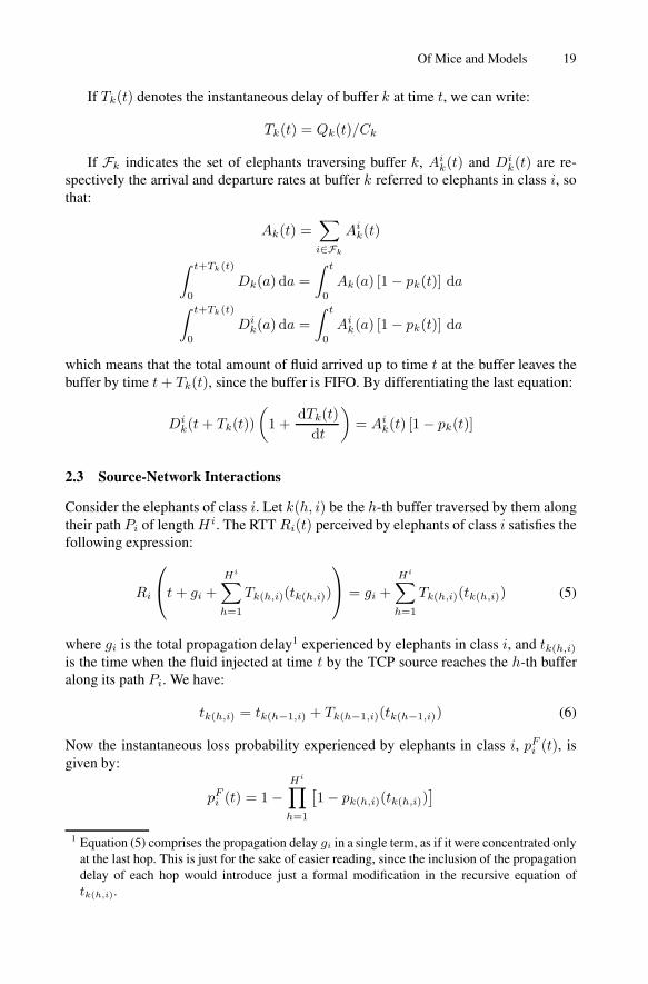
Consider the elephants of class i. Let k(h, i) be the h-th buffer traversed by them alongtheir path Pi of length Hi. The RTT Ri(t) perceived by elephants of class i satisfies thefollowing expression:

Ri

t + gi +

Hi∑h=1

Tk(h,i)(tk(h,i))

= gi +

Hi∑h=1

Tk(h,i)(tk(h,i)) (5)

where gi is the total propagation delay1 experienced by elephants in class i, and tk(h,i)

is the time when the fluid injected at time t by the TCP source reaches the h-th bufferalong its path Pi. We have:

tk(h,i) = tk(h−1,i) + Tk(h−1,i)(tk(h−1,i)) (6)

Now the instantaneous loss probability experienced by elephants in class i, pFi (t), is

given by:

pFi (t) = 1 −

Hi∏h=1

[1 − pk(h,i)(tk(h,i))

]

1 Equation (5) comprises the propagation delay gi in a single term, as if it were concentrated onlyat the last hop. This is just for the sake of easier reading, since the inclusion of the propagationdelay of each hop would introduce just a formal modification in the recursive equation oftk(h,i).

20 Marco Ajmone Marsan et al.

By omitting the class index from the notation, the loss rate indicator λ(w, t) in ourPDFM model can be computed as follows:

λ (w, t + R(t)) =w pF (t)

R(t)(7)

where w/R(t) is the instantaneous emission rate of TCP sources, and the source win-dow at time t + R(t) is used to approximate the window at time t. Intuitively, this lossmodel distributes the lost fluid over the entire population, proportionally to the windowsize.

Finally, in both models:

Ak(t) =∑

i

∑q

riqkDi

q(t) +∑

i

eik

Wi(t)Ri(t)

Ni (8)

where eik = 1 if buffer k is the first buffer traversed by elephants of class i, and 0

otherwise; riqk is derived by the routing matrix, being ri

qk = 1 if buffer k immediatelyfollows buffer q along Pi.

2.4 Mice

The extension of fluid models to a finite population of mice was provided only in [12],thus, here we refer only to the PDFM model.

The model of TCP mice discussed in this section extends the PDFM model reportedin [12], and takes into account the effects of the sources maximum window size Wmax,of the TCP fast recovery mechanism which prevents from halving the window morethan once in each round-trip time, of the initial slow-start phase up to the first loss, andof time-outs.

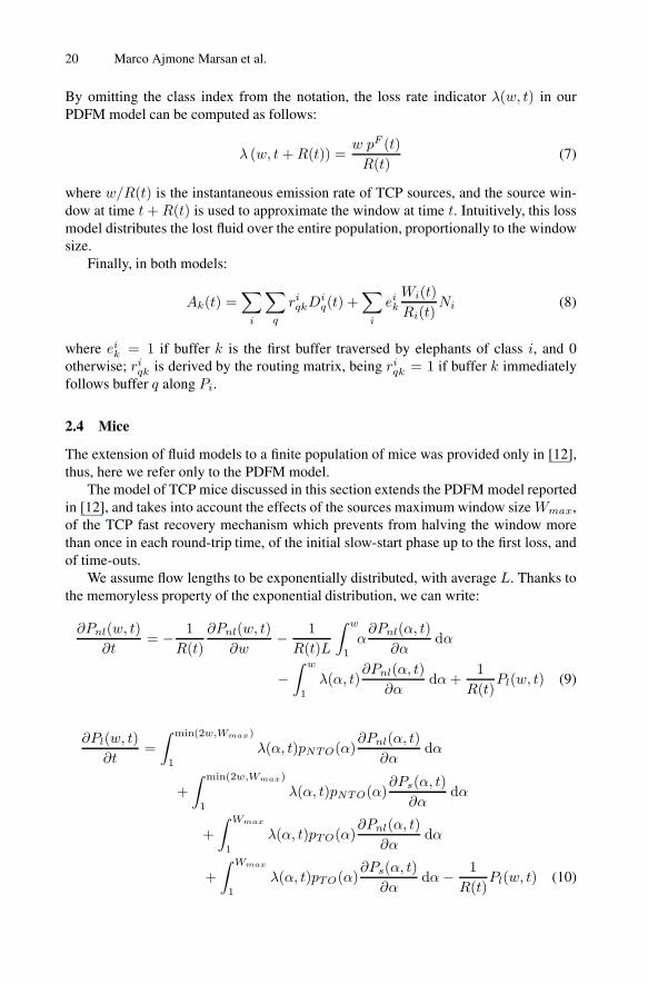
We assume flow lengths to be exponentially distributed, with average L. Thanks tothe memoryless property of the exponential distribution, we can write:

∂Pnl(w, t)∂t

= − 1R(t)

∂Pnl(w, t)∂w

− 1R(t)L

∫ w

1

α∂Pnl(α, t)

∂αdα

−∫ w

1

λ(α, t)∂Pnl(α, t)

∂αdα +

1R(t)

Pl(w, t) (9)

∂Pl(w, t)∂t

=∫ min(2w,Wmax)

1

λ(α, t)pNTO(α)∂Pnl(α, t)

∂αdα

+∫ min(2w,Wmax)

1

λ(α, t)pNTO(α)∂Ps(α, t)

∂αdα

+∫ Wmax

1

λ(α, t)pTO(α)∂Pnl(α, t)

∂αdα

+∫ Wmax

1

λ(α, t)pTO(α)∂Ps(α, t)

∂αdα − 1

R(t)Pl(w, t) (10)

Of Mice and Models 21

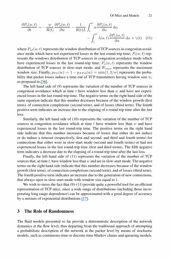
∂Ps(w, t)∂t

= − w

R(t)∂Ps(w, t)

∂w− 1

R(t)L

∫ w

1

α∂Ps(α, t)

∂αdα

−∫ w

1

λ(α, t)∂Ps(α, t)

∂αdα + γ(t) (11)

where Pnl(w, t) represents the window distribution of TCP sources in congestion avoid-ance mode which have not experienced losses in the last round-trip time; Pl(w, t) rep-resents the windows distribution of TCP sources in congestion avoidance mode whichhave experienced losses in the last round-trip time; Ps(w, t) represents the windowdistribution of TCP sources in slow-start mode; and Wmax represents the maximumwindow size. Finally, pTO(w) = 1 − pNTO(w) = min(1, 3/w) represents the proba-bility that packet losses induce a time-out of TCP transmitters having window size w,as proposed in [16].

The left hand side of (9) represents the variation of the number of TCP sources incongestion avoidance which at time t have window less than w and have not experi-enced losses in the last round-trip time. The negative terms on the right hand side of thesame equation indicate that this number decreases because of the window growth (firstterm), of connection completions (second term), and of losses (third term). The fourthpositive term indicates an increase due to the elapsing of a round trip time after the lastloss.

Similarly, the left hand side of (10) represents the variation of the number of TCPsources in congestion avoidance which at time t have window less than w and haveexperienced losses in the last round-trip time. The positive terms on the right handside indicate that this number increases because of losses that either do not induceor do induce a timeout (respectively, first and second, and third and fourth terms) forconnections that either were in slow-start mode (second and fourth terms) or had notexperienced losses in the last round-trip time (first and third terms). The fifth negativeterm indicates a decrease due to the elapsing of a round trip time after the last loss.

Finally, the left hand side of (11) represents the variation of the number of TCPsources that, at time t, have window less than w and are in slow-start mode. The negativeterms on the right hand side indicate that this number decreases because of the windowgrowth (first term), of connection completions (second term), and of losses (third term).The fourth positive term indicates an increase due to the generation of new connections,that always open in slow-start mode with window size equal to 1.

We wish to stress the fact that (9)-(11) provide quite a powerful tool for an efficientrepresentation of TCP mice, since a wide range of distributions (including those incor-porating long range dependence) can be approximated with a good degree of accuracyby a mixture of exponential distributions [17].

3 The Role of Randomness

The fluid models presented so far provide a deterministic description of the networkdynamics at the flow level, thus departing from the traditional approach of attemptinga probabilistic description of the network at the packet level by means of stochasticmodels, such as continuous-time or discrete-time Markov chains and queueing models.

22 Marco Ajmone Marsan et al.

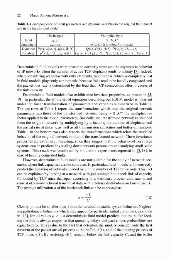
Table 1. Correspondence of input parameters and dynamic variables in the original fluid modeland in the transformed model.

Unchanged Multiplied by η

Input g, L N , B, Cparameters p max γ(t, l), γ(t), min th, max th

Dynamic R(t), λ(w, t), p(t), W (t) Q(t), D(t), A(t), P (w, t), Pmax(t)variables pF (t), T (t), p̄L, w̄(t) PO(w, t), PL(w, t), P (w, t, l), Ps(w, t, l), Ps(w, t)

Deterministic fluid models were proven to correctly represent the asymptotic behaviorof IP networks when the number of active TCP elephants tends to infinity [7]. Indeed,when considering scenarios with only elephants, randomness, which is completely lostin fluid models, plays only a minor role, because links tend to be heavily congested, andthe packet loss rate is determined by the load that TCP connections offer in excess ofthe link capacity.

Deterministic fluid models also exhibit nice invariant properties, as proven in [5,18]. In particular, the whole set of equations describing our PDFM model is invariantunder the linear transformation of parameters and variables summarized in Table 1.The top rows of Table 1 report the transformations which map the original networkparameters into those of the transformed network, being η ∈ IR+ the multiplicativefactor applied to the model parameters. Basically, the transformed network is obtainedfrom the original network by multiplying by a factor η the number of elephants andthe arrival rate of mice γ, as well as all transmission capacities and buffer dimensions.Table 1 in the bottom rows also reports the transformations which relate the modeledbehavior of the original network to that of the transformed network. These invarianceproperties are extremely interesting, since they suggest that the behavior of very largesystems can be predicted by scaling down network parameters and studying small-scalesystems. This result was confirmed by simulation experiments reported in [5, 18], incase of heavily congested links.

However, deterministic fluid models are not suitable for the study of network sce-narios where link capacities are not saturated. In particular, fluid models fail to correctlypredict the behavior of networks loaded by a finite number of TCP mice only. This factcan be explained by looking at a network with just a single bottleneck link of capacityC, loaded by TCP mice that open according to a stationary process with rate γ, andconsist of a unidirectional transfer of data with arbitrary distribution and mean size L.The average utilization ρ of the bottleneck link can be expressed as

ρ =γ L

C(12)

Clearly, ρ must be smaller than 1 in order to obtain a stable system behavior. Neglect-ing pathological behaviors which may appear for particular initial conditions, as shownin [13], for all values ρ < 1 a deterministic fluid model predicts that the buffer feed-ing the link is always empty, so that queueing delays and packet loss probabilities areequal to zero. This is due to the fact that deterministic models consider only the firstmoment of the packet arrival process at the buffer, A(t), and of the opening process ofTCP mice, γ(t). By so doing, A(t) remains below the link capacity C, and the buffer

Of Mice and Models 23

remains empty. Since the loss probability is zero, no retransmissions are needed, andthe actual traffic intensity on the link converges to the nominal link utilization ρ com-puted by (12). This prediction is very far from what is observed in either ns-2 simulationexperiments or measurement setups, that show how queuing delays and packet lossesare non-negligible for a wide range of values ρ < 1. This prediction error is essentiallydue to the fact that, in underload conditions, randomness plays a fundamental role thatcannot be neglected in the description of the network dynamics. Indeed, randomnessimpacts the system behavior at two different levels:

– Randomness at Flow Level is due to the stochastic nature of the arrival and com-pletion processes of TCP mice. The number of active TCP mice in the networkvaries over time, and the offered load changes accordingly.

– Randomness at Packet Level is due to the stochastic nature of the arrival anddeparture processes of packets at buffers. In particular, the burstiness of TCP trafficis responsible for high queueing delays and sporadic buffer overloads, even whenthe average link utilization is much smaller than 1.

3.1 The Hybrid Fluid-Montecarlo Approach

The approach we propose to account for randomness consists in transforming the deter-ministic differential equations of the fluid model into stochastic differential equations,which are then solved using a Montecarlo approach.

More in detail, we consider two levels of randomness:– Randomness at Flow Level. The deterministic mice arrival rate γ(t) in (10) is re-

placed by a Poisson counter with average γ(t). The deterministic mice completionprocess can be replaced by an inhomogeneous Poisson process whose average attime t is represented by the sum of the second terms on the right hand side of (9) and(11). As opposed to the mice arrival process, which is assumed to be exogenous,the mice completion process depends on the network congestion: when the packetloss probability increases, the rate at which mice leave the system is reduced.

– Randomness at Packet Level. The workload emitted by TCP sources, rather thanbeing a continuous deterministic fluid process with rate Wi(t)Ni/Ri(t), can betaken to be a stochastic point process with the same rate. Previous work in TCPmodeling [19, 20] showed that an effective description of TCP traffic in networkswith high bandwidth-delay product is obtained by means of a batched Poisson pro-cess in which the batch size is distributed according to the window size of TCPsources. The intuition behind this result is that, if the transmission time for allpackets in a window is much smaller than the round trip time, packets transmis-sions are clustered at the beginning of each RTT. This introduces a high correlationin the inter-arrival times of packets at routers, that cannot be neglected, since itheavily impacts the buffer behavior. By grouping together all packets sent in a RTTas a single batch, we are able to capture most of the bursty nature of TCP traffic.This approach is very well suited to our model, which describes the window sizedistribution of TCP sources.

An important observation is that the addition of randomness in the model destroysthe invariance properties described in Section 3. This can be explained very simply byconsidering that the loss probability predicted by any analytical model of a finite queue

24 Marco Ajmone Marsan et al.

with random arrivals (e.g., an M/M/1/B queue) depends on the buffer size, usually in anon linear way. Instead, according to the transformations of Table 1, the loss probabilityshould remain the same after scaling the buffer size. In underload conditions, it is clearlywrong to assume that the packet loss probability does not change with variations in thebuffer size.

4 Results for Mice

In this section we discuss results for network scenarios comprising TCP mice. First, weinvestigate the impact of the source emission model in a scenario where only mice areactive. Second, we study the impact of the flow size distribution. Third, we investigatethe invariance properties of the network when mice are present. Finally we study adynamic (non-stationary) scenario in which a link is temporarily overloaded by a flashcrowd of new TCP connection requests.

4.1 Impact of the Source Emission Model

Consider a single bottleneck link fed by a drop-tail buffer, with capacity equal to 1000packets. The link data rate C is 1.0 Gbps, while the propagation delay between TCPsources and buffer is 30 ms. In order to reproduce a TCP traffic load close to what hasbeen observed on the Internet, flow sizes are distributed according to a Pareto distribu-tion with shape parameter equal to 1.2 and scale parameter equal to 4.

Using the algorithm proposed in [17], we approximated the Pareto distribution witha hyper-exponential distribution of the 9-th order, whose parameters are reported inTable 2. The resulting average flow length is 20.32 packets. Correspondingly, 9 classesof TCP mice are considered in our model. The maximum window size is set to 64packets for all TCP sources. Experiments with loads equal to 0.6, 0.8 and 0.9 were run;however, for the sake of brevity, we report here only the results for load equal to 0.9.

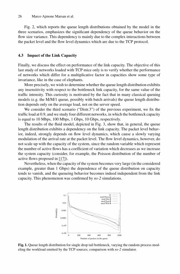
Fig. 1 compares the queue lengths distributions obtained with ns-2, and with thestochastic fluid model. While in the model the flow arrival and completion processeshave been randomized according to a non-homogeneous Poisson process (see Section3.1), different approaches have been tried to model the traffic emitted by sources:

– Poisson: the emitted traffic is a Poisson process with time-varying rate;– Det-B: the emitted traffic is a batch Poisson process with time-varying rate and

constant batch size, equal to the instantaneous average TCP mice window size;– Exp-B: the emitted traffic is a batch Poisson process with time-varying rate and

exponential batch size, whose mean is equal to the instantaneous average TCP micewindow size;

– Win-B: the emitted traffic is a batch Poisson process with time-varying rate, inwhich the batch size distribution is equal to the instantaneous TCP mice windowsize distribution.

The last three approaches were suggested by recent results about the close relation-ship existing between the burstiness of the traffic generated by mice and their windowsize [19].

Of Mice and Models 25

Table 2. Parameters of the hyper-exponential distribution approximating the Pareto distribution.

Prob. mean length

7.88 10−1 6.481.65 10−1 23.263.70 10−2 80.658.34 10−3 279.71.87 10−3 970.24.22 10−4 33769.46 10−5 118622.10 10−5 430864.52 10−6 176198

If we use a Poisson process to model the instants in which packets (or, more pre-cisely, units of fluid) are emitted by TCP sources, the results generated by the fluidmodel cannot match the results obtained with the ns-2 simulator, as can be observed inFig. 1. Instead, the performance predictions obtained with the fluid model become quiteaccurate when the workload emitted by TCP sources is taken to be a Poisson processwith batch arrivals. The best fitting (confirmed also by several other experiments, notreported here for lack of space) is obtained for batch size distribution equal to the instan-taneous TCP mice window size distribution (case Win-B). Note that our proposed classof fluid models naturally provides the information about the window size distribution,whereas the MGT model provides only the average window size.

Table 3 reports the average loss probability, the average queue length, and the av-erage completion time for each class of TCP mice, obtained with ns-2, with the Pois-son and the Win-B models. The Poisson model significantly underestimates the averagequeue length and loss probability, thus producing an optimistic prediction of comple-tion times. The Win-B model moderately overestimates the average queue length andloss probability, as pointed out in [19]. However, for very short flows, completion timepredictions obtained with the Win-B model are slightly optimistic; this is mainly due tothe fact that an idealized TCP behavior (in particular, without timeouts) is consideredin the model.

4.2 Impact of the Flow Size

We now discuss the ability of our model to capture the impact on the network behaviorof the flow size variance.

We consider three different scenarios, in which flow lengths are distributed accord-ing to either an exponential distribution (“Distr.1”), or hyper-exponentials of the secondorder (“Distr.2” and “Distr.3”). For all three scenarios, we keep the average flow sizeequal to 20.32 (this is the average flow size used in the previous subsection), and wevary the standard deviation σ. Detailed parameters of our experiments are reported inTable 4.

Table 5 shows a comparison between the results obtained with the Win-B model andwith ns-2. As in previous experiments, the model moderately overestimates both theaverage loss probability and the average queue length. The discrepancies in the averagecompletion times between model and ns-2 remain within 10%.

26 Marco Ajmone Marsan et al.

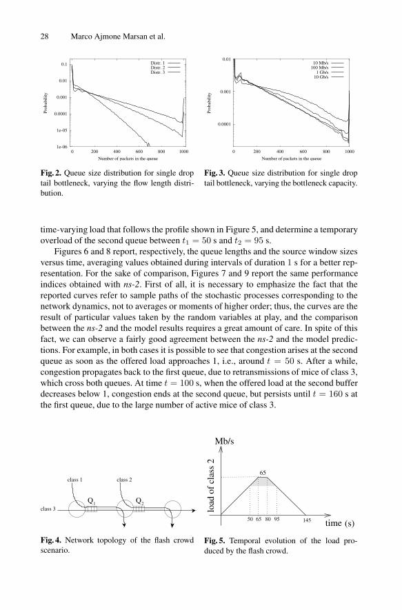
Fig. 2, which reports the queue length distributions obtained by the model in thethree scenarios, emphasizes the significant dependency of the queue behavior on theflow size variance. This dependency is mainly due to the complex interactions betweenthe packet level and the flow level dynamics which are due to the TCP protocol.

4.3 Impact of the Link Capacity

Finally, we discuss the effect on performance of the link capacity. The objective of thislast study of networks loaded with TCP mice only is to verify whether the performanceof networks which differ for a multiplicative factor in capacities show some type ofinvariance, like in the case of elephants.

More precisely, we wish to determine whether the queue length distribution exhibitsany insensitivity with respect to the bottleneck link capacity, for the same value of thetraffic intensity. This curiosity is motivated by the fact that in many classical queuingmodels (e.g. the M/M/1 queue, possibly with batch arrivals) the queue length distribu-tion depends only on the average load, not on the server speed.

We consider the third scenario (“Distr.3”) of the previous experiment, we fix thetraffic load at 0.9, and we study four different networks, in which the bottleneck capacityis equal to 10 Mbps, 100 Mbps, 1 Gbps, 10 Gbps, respectively.

The results of the fluid model, depicted in Fig. 3, show that, in general, the queuelength distribution exhibits a dependency on the link capacity. The packet level behav-ior, indeed, strongly depends on flow level dynamics, which cause a slowly varyingmodulation of the arrival rate at the packet level. The flow level dynamics, however, donot scale up with the capacity of the system, since the random variable which representthe number of active flows has a coefficient of variation which decreases as we increasethe system capacity (consider, for example, the Poisson distribution of the number ofactive flows proposed in [17]).

Nevertheless, when the capacity of the system becomes very large (in the consideredexample, greater than 1 Gbps) the dependence of the queue distribution on capacitytends to vanish, and the queueing behavior becomes indeed independent from the linkcapacity. This phenomenon was confirmed by ns-2 simulations.

1e-06

1e-05

0.0001

0.001

0.01

0.1

0 200 400 600 800 1000

Prob

abili

ty

Number of packets in the queue

nsmod Poisson

mod Det-Bmod Exp-Bmod Win-B

Fig. 1. Queue length distribution for single drop tail bottleneck, varying the random process mod-eling the workload emitted by the TCP sources; comparison with ns-2 simulator.

Of Mice and Models 27

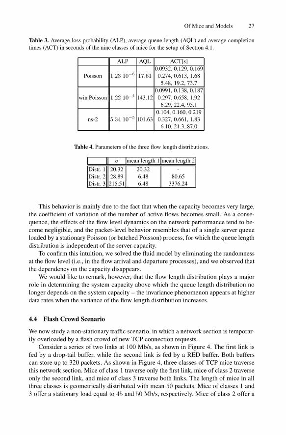
Table 3. Average loss probability (ALP), average queue length (AQL) and average completiontimes (ACT) in seconds of the nine classes of mice for the setup of Section 4.1.

ALP AQL ACT[s]0.0932, 0.129, 0.169

Poisson 1.23 10−6 17.61 0.274, 0.613, 1.685.48, 19.2, 73.7

0.0991, 0.138, 0.187win Poisson 1.22 10−4 143.12 0.297, 0.658, 1.92

6.29, 22.4, 95.10.104, 0.160, 0.219

ns-2 5.34 10−5 101.63 0.327, 0.661, 1.836.10, 21.3, 87.0

Table 4. Parameters of the three flow length distributions.

σ mean length 1 mean length 2

Distr. 1 20.32 20.32 -Distr. 2 28.89 6.48 80.65Distr. 3 215.51 6.48 3376.24

This behavior is mainly due to the fact that when the capacity becomes very large,the coefficient of variation of the number of active flows becomes small. As a conse-quence, the effects of the flow level dynamics on the network performance tend to be-come negligible, and the packet-level behavior resembles that of a single server queueloaded by a stationary Poisson (or batched Poisson) process, for which the queue lengthdistribution is independent of the server capacity.

To confirm this intuition, we solved the fluid model by eliminating the randomnessat the flow level (i.e., in the flow arrival and departure processes), and we observed thatthe dependency on the capacity disappears.

We would like to remark, however, that the flow length distribution plays a majorrole in determining the system capacity above which the queue length distribution nolonger depends on the system capacity – the invariance phenomenon appears at higherdata rates when the variance of the flow length distribution increases.

4.4 Flash Crowd Scenario

We now study a non-stationary traffic scenario, in which a network section is temporar-ily overloaded by a flash crowd of new TCP connection requests.

Consider a series of two links at 100 Mb/s, as shown in Figure 4. The first link isfed by a drop-tail buffer, while the second link is fed by a RED buffer. Both bufferscan store up to 320 packets. As shown in Figure 4, three classes of TCP mice traversethis network section. Mice of class 1 traverse only the first link, mice of class 2 traverseonly the second link, and mice of class 3 traverse both links. The length of mice in allthree classes is geometrically distributed with mean 50 packets. Mice of classes 1 and3 offer a stationary load equal to 45 and 50 Mb/s, respectively. Mice of class 2 offer a

28 Marco Ajmone Marsan et al.

1e-06

1e-05

0.0001

0.001

0.01

0.1

0 200 400 600 800 1000

Prob

abili

ty

Number of packets in the queue

Distr. 1Distr. 2Distr. 3

Fig. 2. Queue size distribution for single droptail bottleneck, varying the flow length distri-bution.

0.0001

0.001

0.01

0 200 400 600 800 1000

Prob

abili

ty

Number of packets in the queue

10 Mb/s100 Mb/s

1 Gb/s 10 Gb/s

Fig. 3. Queue size distribution for single droptail bottleneck, varying the bottleneck capacity.

time-varying load that follows the profile shown in Figure 5, and determine a temporaryoverload of the second queue between t1 = 50 s and t2 = 95 s.

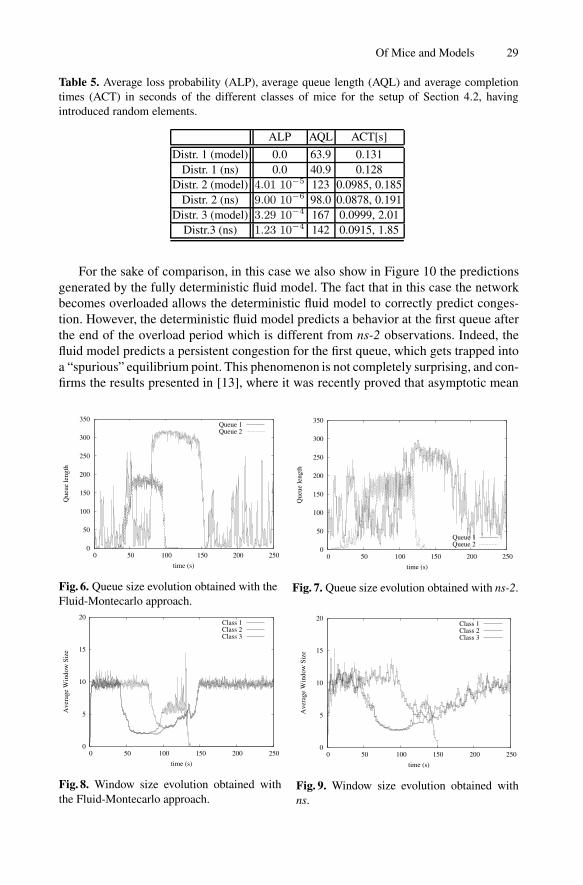
Figures 6 and 8 report, respectively, the queue lengths and the source window sizesversus time, averaging values obtained during intervals of duration 1 s for a better rep-resentation. For the sake of comparison, Figures 7 and 9 report the same performanceindices obtained with ns-2. First of all, it is necessary to emphasize the fact that thereported curves refer to sample paths of the stochastic processes corresponding to thenetwork dynamics, not to averages or moments of higher order; thus, the curves are theresult of particular values taken by the random variables at play, and the comparisonbetween the ns-2 and the model results requires a great amount of care. In spite of thisfact, we can observe a fairly good agreement between the ns-2 and the model predic-tions. For example, in both cases it is possible to see that congestion arises at the secondqueue as soon as the offered load approaches 1, i.e., around t = 50 s. After a while,congestion propagates back to the first queue, due to retransmissions of mice of class 3,which cross both queues. At time t = 100 s, when the offered load at the second bufferdecreases below 1, congestion ends at the second queue, but persists until t = 160 s atthe first queue, due to the large number of active mice of class 3.

Q Q1 2

class 1 class 2

class 3

Fig. 4. Network topology of the flash crowdscenario.

time

load

of

clas

s 2

65

Mb/s

(s)145806550 95

Fig. 5. Temporal evolution of the load pro-duced by the flash crowd.

Of Mice and Models 29

Table 5. Average loss probability (ALP), average queue length (AQL) and average completiontimes (ACT) in seconds of the different classes of mice for the setup of Section 4.2, havingintroduced random elements.

ALP AQL ACT[s]

Distr. 1 (model) 0.0 63.9 0.131Distr. 1 (ns) 0.0 40.9 0.128

Distr. 2 (model) 4.01 10−5 123 0.0985, 0.185Distr. 2 (ns) 9.00 10−6 98.0 0.0878, 0.191

Distr. 3 (model) 3.29 10−4 167 0.0999, 2.01Distr.3 (ns) 1.23 10−4 142 0.0915, 1.85

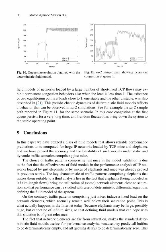
For the sake of comparison, in this case we also show in Figure 10 the predictionsgenerated by the fully deterministic fluid model. The fact that in this case the networkbecomes overloaded allows the deterministic fluid model to correctly predict conges-tion. However, the deterministic fluid model predicts a behavior at the first queue afterthe end of the overload period which is different from ns-2 observations. Indeed, thefluid model predicts a persistent congestion for the first queue, which gets trapped intoa “spurious” equilibrium point. This phenomenon is not completely surprising, and con-firms the results presented in [13], where it was recently proved that asymptotic mean

0

50

100

150

200

250

300

350

0 50 100 150 200 250

Que

ue le

ngth

time (s)

Queue 1Queue 2

Fig. 6. Queue size evolution obtained with theFluid-Montecarlo approach.

0

50

100

150

200

250

300

350

0 50 100 150 200 250

Que

ue le

ngth

time (s)

Queue 1Queue 2

Fig. 7. Queue size evolution obtained with ns-2.

0

5

10

15

20

0 50 100 150 200 250

Ave

rage

Win

dow

Siz

e

time (s)

Class 1Class 2Class 3

Fig. 8. Window size evolution obtained withthe Fluid-Montecarlo approach.

0

5

10

15

20

0 50 100 150 200 250

Ave

rage

Win

dow

Siz

e

time (s)

Class 1Class 2Class 3

Fig. 9. Window size evolution obtained withns.

30 Marco Ajmone Marsan et al.

0

50

100

150

200

250

300

350

0 50 100 150 200 250

Que

ue le

ngth

time (s)

Queue 1Queue 2

Fig. 10. Queue size evolution obtained with thedeterministic fluid model.

0

50

100

150

200

250

300

350

0 50 100 150 200 250

Que

ue le

ngth

time (s)

Queue 1Queue 2

Fig. 11. ns-2 sample path showing persistentcongestion at queue 1.

field models of networks loaded by a large number of short-lived TCP flows may ex-hibit permanent congestion behaviors also when the load is less than 1. The existenceof two equilibrium points at loads close to 1, one stable and the other unstable, was alsodescribed in [21]. This pseudo-chaotic dynamics of deterministic fluid models reflectsa behavior that can be observed in ns-2 simulations. See for example the ns-2 samplepath reported in Figure 11, for the same scenario. In this case congestion at the firstqueue persists for a very long time, until random fluctuations bring down the system tothe stable operating point.

5 Conclusions

In this paper we have defined a class of fluid models that allows reliable performancepredictions to be computed for large IP networks loaded by TCP mice and elephants,and we have proved the accuracy and the flexibility of such models under static anddynamic traffic scenarios comprising just mice.

The choice of traffic patterns comprising just mice in the model validation is dueto the fact that the effectiveness of fluid models in the performance analysis of IP net-works loaded by just elephants or by mixes of elephants and mice was already provedin previous works. The key characteristic of traffic patterns comprising elephants thatmakes them suitable to a fluid analysis lies in the fact that elephants (being modeled asinfinite-length flows) bring the utilization of (some) network elements close to satura-tion, so that performance can be studied with a set of deterministic differential equationsdefining the fluid model of the system.

On the contrary, traffic patterns comprising just mice, induce a fixed load on thenetwork elements, which normally remain well below their saturation point. This iswhat actually happens in the Internet today (because elephants may be large, possiblyhuge, but cannot be of infinite size), so that defining fluid models that can cope withthis situation is of great relevance.

The fact that network elements are far from saturation, makes the standard deter-ministic fluid models useless for performance analysis, because they predict all buffersto be deterministically empty, and all queuing delays to be deterministically zero. This

Of Mice and Models 31

is not what we experience and measure from the Internet. The reason for this discrep-ancy lies in the stochastic nature of traffic, which is present on the Internet, but is notreflected by the standard deterministic fluid models.

The fluid model paradigm that we defined in this paper is capable of accountingfor randomness in traffic, at both the flow and the packet levels, and can thus producereliable performance predictions for networks that operate far from saturation.

The accuracy and the flexibility of the modeling paradigm was proved by consid-ering both static traffic patterns, from which equilibrium behaviors can be studied, anddynamic traffic conditions, that allow the investigation of transient dynamics.

References

1. V.Misra, W.Gong, D.Towsley, “Stochastic Differential Equation Modeling and Analysis ofTCP Window Size Behavior”, Performance’99, Istanbul, Turkey, October 1999.

2. V.Misra, W.B.Gong, D. Towsley, “Fluid-Based Analysis of a Network of AQM Routers Sup-porting TCP Flows with an Application to RED”, ACM SIGCOMM 2000, Stockholm, Swe-den, August 2000.

3. Y.Liu, F.Lo Presti, V.Misra, D.Towsley, “Fluid Models and Solutions for Large-Scale IPNetworks”, ACM SIGMETRICS 2003, San Diego, CA, USA, June 2003.

4. C.V.Hollot, Y.Liu, V.Misra and D.Towsley, “Unresponsive Flows and AQM Performance,”IEEE Infocom 2003, San Francisco, CA, USA, March 2003.

5. R.Pan, B.Prabhakar, K.Psounis, D.Wischik, “SHRiNK: A Method for Scalable PerformancePrediction and Efficient Network Simulation”, IEEE Infocom 2003, San Francisco, CA,USA, March 2003.

6. S.Deb, S.Shakkottai, R.Srikant, “Stability and Convergence of TCP-like Congestion Con-trollers in a Many-Flows Regime”, IEEE Infocom 2003, San Francisco, CA, USA, March2003.

7. P.Tinnakornsrisuphap, A.Makowski, “Limit Behavior of ECN/RED Gateways Under a LargeNumber of TCP Flows”, IEEE Infocom 2003, San Francisco, CA, USA, March 2003.

8. M.Barbera, A.Lombardo, G.Schembra, “A Fluid-Model of Time-Limited TCP flows”, toappear on Computer Networks.

9. F.Baccelli, D.Hong, “Interaction of TCP Flows as Billiards”, IEEE Infocom 2003, San Fran-cisco, CA, USA, March 2003.

10. F.Baccelli, D.Hong, “Flow Level Simulation of Large IP Networks”, IEEE Infocom 2003,San Francisco, CA, USA, March 2003.

11. F.Baccelli, D.R.McDonald, J.Reynier, “A Mean-Field Model for Multiple TCP Connectionsthrough a Buffer Implementing RED”, Performance Evaluation, vol. 49 n. 1/4, pp. 77-97,2002.

12. M.Ajmone Marsan, M.Garetto, P.Giaccone, E.Leonardi, E.Schiattarella, A.Tarello, “UsingPartial Differential Equations to Model TCP Mice and Elephants in Large IP Networks”,IEEE Infocom 2004, Hong Kong, March 2004.

13. F.Baccelli, A.Chaintreau, D.Mc Donald, D.De Vleeschauwer, “A Mean Field Analysis ofInteracting HTTP Flows”, ACM SIGMETRICS 2004, New York, NY, June 2004.

14. G.Carofiglio, E.Leonardi, M.Garetto, M.Ajmone Marsan, A.Tarello, “Beyond Fluid Models:Modelling TCP Mice in IP Networks with Non-Stationary Random Traffic”, submitted forpublication.

15. S.Floyd, V.Jacobson, “Random Early Detection Gateways for Congestion Avoidance”,IEEE/ACM Transactions on Networking, vol. 1, n. 4, pp. 397-413, August 1993.

32 Marco Ajmone Marsan et al.

16. J.Padhye, V.Firoiu, D.Towsley, and J.Kurose, “Modeling TCP Throughput: A Simple Modeland its Empirical Validation,” ACM SIGCOMM’98 - ACM Computer Communication Re-view, 28(4):303–314, September 1998.

17. A.Feldmann, W.Whitt, “Fitting Mixtures of Exponentials to Long-Tail Distributions to Ana-lyze Network Performance Models”, IEEE Infocom 97, Kobe, Japan, April 1997.

18. M.Ajmone Marsan, M.Garetto, P.Giaccone, E.Leonardi, E.Schiattarella, A.Tarello, ”UsingPartial Differential Equations to Model TCP Mice and Elephants in Large IP Networks”,Technical report available at http://www.telematics.polito.it/garetto/papers/TON-2004-leonardi.ps

19. M.Garetto, D.Towsley, “Modeling, Simulation and Measurements of Queuing Delay UnderLong-Tail Internet Traffic”, ACM SIGMETRICS 2003, San Diego, CA, USA, June 2003.

20. M.Garetto, R.Lo Cigno, M.Meo, M.Ajmone Marsan, “Modeling Short-Lived TCP Connec-tions with Open Multiclass Queuing Networks”, Computer Networks Journal, vol. 44, n. 2,pp. 153–176, February 2004.

21. M.Meo, M.Garetto, M.Ajmone Marsan, R.Lo Cigno, “On the Use of Fixed Point Approx-imations to Study Reliable Protocols over Congested Links”, IEEE Globecom 2003, SanFrancisco, CA, December 2003.