Embed Size (px)
Citation preview

EXPERIMENTAL AND MODELLING STUDIES OF
CORROSION FATIGUE DAMAGE IN A LINEPIPE STEEL
A thesis submitted to the University of Manchester for the degree of
Doctor of Philosophy
in the Faculty of Engineering and Physical Sciences
2015
Olusegun Fatoba
School of Materials

2
Table of Contents
Chapter 1 Introduction ............................................................................................ 9
1.1 Background .................................................................................................... 10
1.2 Aims and objectives ....................................................................................... 11
1.3 Thesis outline ................................................................................................. 12
Chapter 2 Literature Review ................................................................................... 13
2.1 Corrosion Damage ......................................................................................... 14
2.2 Fatigue of Metals............................................................................................ 18
2.3 Fatigue Life Prediction .................................................................................. 21
2.4 Behaviour of Short Fatigue Cracks ............................................................... 26
2.5 Fatigue Limit and Non-Propagating Cracks................................................ 32
2.6 Kitagawa-Takahashi Diagram ...................................................................... 33
2.7 Environment Assisted Fatigue ...................................................................... 37
2.8 Crack Nucleation from Corrosion Pits ......................................................... 48
2.9 Corrosion Fatigue Lifetime Modelling ......................................................... 52
Chapter 3 Experimental Methods .......................................................................... 58
3.1 Introduction ................................................................................................... 59
3.2 Material........................................................................................................... 59
3.3 Chemical composition ................................................................................... 60
3.4 Metallography ................................................................................................ 60
3.5 Micro-hardness .............................................................................................. 61
3.6 Electrochemical Testing ................................................................................. 61
3.7 Rationale for use of single artificial pits ....................................................... 63
3.8 Simulation of pit growth ............................................................................... 63
3.9 Mechanical Testing ........................................................................................ 71
3.10 Crack growth measurements ...................................................................... 79
3.11 Image analysis and fractography................................................................ 80
Chapter 4 Modelling Methods ............................................................................... 81
4.1 Introduction ................................................................................................... 82
4.2 FEA modelling techniques ............................................................................ 82
4.3 Analysis of stresses and strains around pits ................................................ 88
4.4 Modelling of the interaction between localised corrosion and stress ........ 90

3
Chapter 5 Experimental Results and Discussion ................................................ 98
5.1 Introduction ................................................................................................... 99
5.2 Material Characterisation .............................................................................. 99
5.3 Stress-strain properties .................................................................................. 102
5.4 Pit growth behaviour ..................................................................................... 109
5.5 Fatigue and corrosion fatigue behaviour ..................................................... 112
5.6 Fracture surface analysis ............................................................................... 145
5.7 Stress-life (S-N) curves .................................................................................. 151
Chapter 6 Finite Element Analysis Results and Discussion............................... 155
6.1 Introduction ................................................................................................... 156
6.2 Mesh convergence study ............................................................................... 157
6.3 Model validation ............................................................................................ 157
6.4 Changes in stress and strain distribution due to pit growth ...................... 159
6.5 Analyses of stress and strain distribution in artificial pits ......................... 169
6.6 Effect of pit-to-pit proximity on stress and strain distribution .................. 173
Chapter 7 CAFE Modelling Results and Discussion .......................................... 179
7.1 Introduction ................................................................................................... 180
7.2 Simulation of the micro-capillary cell .......................................................... 181
7.3 Model parameter sensitivity analysis........................................................... 182
7.4 Influence of model parameters ..................................................................... 186
7.5 Model validation ............................................................................................ 190
7.6 Evolution of pit depth with and without stress .......................................... 195
7.7 Evolution of stress and strain with time ...................................................... 197
7.8 Preliminary results from 3-D cellular automata model .............................. 201
Chapter 8 Fatigue Lifetime Modelling .................................................................. 204
8.1 Introduction ................................................................................................... 205
8.2 Multi-stage damage accumulation model ................................................... 205
8.3 Discussion ...................................................................................................... 226
Chapter 9 General Discussion ................................................................................ 229
9.1 Introduction ................................................................................................... 230
9.2 The fatigue limit ............................................................................................. 230
9.3 Influence of pit size on fatigue strength ....................................................... 231
9.4 Effect of stress on pit development .............................................................. 236
9.5 Pit-to-crack transition behaviour .................................................................. 238

4
9.6 Crack propagation behaviour ....................................................................... 247
9.7 Re-assessment of pit-to-crack transition criteria ......................................... 252
Chapter 10 Conclusions ........................................................................................... 253
Chapter 11 Future Work .......................................................................................... 256
11.1 Experimental work ...................................................................................... 257
11.2 Modelling work............................................................................................ 258
References………………………………………………………………………….259
Appendix………………………………….………………………………………..274

5
NOMENCLATURE
The frequently used acronyms and symbols are listed below. Those which are rarely used
are defined in their context.
𝑎𝑐𝑒: crack extension from pit
API: American Petroleum Institute
ARp: Pit aspect ratio
ARp,avg: Pit aspect ratio
CA – Cellular automata
CAFE – Cellular automata finite element
CF – Corrosion fatigue
CI – Crack initiation
CPZ – Crack propagation zone
cp: Half pit width
dp: Pit depth
dp,avg: Average pit depth
dth: Threshold separation distance between double pits
f: Cyclic frequency
F: Faraday’s constant
FEA – Finite element analysis
FFZ – Fast fracture zone
HSLA: High strength low alloy
HV: Vickers hardness number
ΔK: Stress intensity factor range
ΔKth: Threshold stress intensity factor range
KDF: Corrosion fatigue knockdown factor
LEFM: Linear elastic fracture mechanics
𝑁𝑓: Fatigue lifetime
𝑁𝑖: Crack initiation lifetime
𝑁𝑖,𝑑𝑜𝑢𝑏𝑙𝑒 : Crack initiation lifetime for double pits
𝑁𝑖,𝑠𝑖𝑛𝑔𝑙𝑒: Crack initiation lifetime for a single pit
R: Stress ratio
𝑠𝑐𝑐: Center-to-center distance between double pits
𝑠𝑒𝑒: Edge-to-edge distance between double pits
Δε: Total strain range
Δσ: Stress range
𝜎𝐹𝐿: Fatigue limit

6
“Experimental and Modelling Studies of Corrosion Fatigue Damage in a Linepipe Steel”.
Olusegun Fatoba, Doctor of Philosophy, The University of Manchester, 2015.
ABSTRACT
The work is concerned with the development of a multi-stage corrosion fatigue lifetime
model, with emphasis on pitting as a precursor to cracking. The model is based upon the
quantitative evaluation of damage during the overall corrosion fatigue process.
The fatigue response of as-received API 5L X65 linepipe steel has been investigated in
terms of the evolution of damage during pit development, pit-to-crack transition and
crack propagation. Micro-potentiostatic polarisation was conducted to evaluate role of
stress on pit development. Crack growth rate measurements were conducted on pre-
pitted specimens, which were tested in air and brine, to evaluate the initiation and
propagation behaviour of cracks emanating from artificial pits. Finite element analysis
was undertaken to evaluate the stress and strain distribution associated with the pits. A
cellular automata finite element model was also developed for predicting corrosion
fatigue damage.
Pit growth rate was enhanced under stress. It was considered that the strain localisation
effect of the pit facilitated strain-assisted dissolution. In air, cracks initiated
predominantly from the pit mouth. FEA results indicated that this was due to localisation
of strain towards the pit mouth. In corrosion fatigue, cracks tended to initiate at the pit
base at low stress and at the pit mouth at higher stresses. Crack initiation lifetimes were
shorter in the aggressive environment compared to air and the effect of the environment
on crack initiation lifetime was lower at higher stress levels. Crack initiation lifetime for
double pits generally decreased with decreasing pit-to-pit separation distance.
The microstructure was observed to influence crack growth behaviour in air particularly
in the early stages when cracks were short. The acceleration and retardation in crack
growth were attributed to the resistance of grain boundaries to crack advance. Cracks
sometimes arrested at these barriers and became non-propagating. Introduction of the
environment for a short period appear to eliminate the resistance of the microstructural
barriers thus promoting re-propagation of the previously arrested crack. The continued
crack propagation after the removal of the environment suggests that the influence of the
environment is more important in the early stages of crack growth. Crack growth rates
were higher in the aggressive environment than in air. The degree of environmental
enhancement of crack growth was found to be greater at lower stress levels and at short
crack lengths. Oxide-induced crack closure and crack coalescence were two mechanisms
that also affected crack growth behaviour.
2-D cellular automata finite element simulation results, with and without stress, show
good agreement agreed with experiments i.e. pit depth and pit aspect ratio increase with
time. Results from 3-D cellular automata simulations of pits are also consistent with
experiments.
Fatigue lifetimes were significantly shorter (i) in the brine environment than in air and (ii)
for specimens with double pits compared to single pits of similar depth. Fatigue strength
in air was found to decrease with increasing pit depth. Corrosion fatigue lifetimes
predicted based upon the developed model showed good agreement with the
experimental lifetimes.

7
DECLARATION
I declare that no portion of the work referred to in this thesis has been submitted in
support of an application for another degree or qualification of this or any other
university or other institution of learning.
Signature
COPYRIGHT
i. The author of this thesis (including any appendices and/or schedules to this thesis)
owns any copyright in it (the “Copyright”) and s/he has given The University of
Manchester the right to use such Copyright for any administrative, promotional,
educational and/or teaching purposes.
ii. Copies of this thesis, either in full or in extracts and whether in hard or electronic
copy, may be made only in accordance with the Copyright, Designs and Patents
Act 1988 (as amended) and regulations issued under it or, where appropriate, in
accordance with licensing agreements which the University has from time to time.
This page must form part of any such copies made.
iii. The ownership of any patents, designs, trademarks and any and all other
intellectual property rights except for the Copyright (the “Intellectual Property
Rights”) and any reproductions of copyright works, for example graphs and tables
(“Reproductions”), which may be described in this thesis, may not be owned by
the author and may be owned by third parties. Such Intellectual Property Rights
and Reproductions cannot and must not be made available for use without the
prior written permission of the owner(s) of the relevant Intellectual Property
Rights and/or Reproductions.
iv. Further information on the conditions under which disclosure, publication and
exploitation of this thesis, the Copyright and any Intellectual Property Rights
and/or Reproductions described in it may take place is available in the University
IP Policy, in any relevant Thesis restriction declarations deposited in the
University Library, The University Library’s regulations and in The University’s
policy on Presentation of Theses.

8
ACKNOWLEDGEMENT
I would like to gratefully acknowledge my supervisor, Professor Robert Akid, whose
invaluable guidance, continuous support, kindness, suggestions and constructive
criticisms throughout this research work and during thesis writing, have helped me to
accomplish my academic goals at this level of study.
I would like to thank the School of Materials, Corrosion Protection Centre and the School
of Mechanical, Aerospace and Civil Engineering for the use of laboratory and mechanical
testing facilities.
I am indebted to BP for providing me with full sponsorship funding for this research
work and for providing the test material.
I would like to thank Dr Rafael Leiva-Garcia for his help in developing the CAFE model
and support in using the confocal microscope. I also thank him for his advice and
suggestions during my research and availability for discussion.
I would like to thank Christopher Evans for developing the micro-capillary cell that was
used in generating corrosion pits on the test samples and for providing DIC results that
were used for FEA model validation.
I am thankful to Stuart Morse and David Mortimer for providing technical support
during mechanical testing, Mark Harris and Ian Winstanley who manufactured the
specimens and Teruo Hashimoto for his support on scanning electron microscopy.
Thanks are also due to other staff in the School of Materials and Corrosion Protection
Centre, especially Olwen Richert, Paul Jordan, Steve Blatch and Harry Pickford for their
support in various forms.
I would like to thank Dr Nicolas Larrosa for his assistance with the use of Abaqus
software and with the writing python scripts that were used in the CAFE model.
I am also thankful Dr D. Engelberg and Dr R. Lindsay and Dr Y. Yang for the advice and
suggestions they provided.
I am grateful to my mother for her prayers and encouragement, and my siblings –
Olawale, Kimberly, Olumuyiwa, Onikepeju, Olanrewaju, Iyanuoluwa and Faith, for their
moral support and prayers. I am also grateful to Taiwo Oguntayo, Femi Akanbi and
Sheilla Osondu-Iheke, for their immeasurable support in the last twelve months.
Last but not least, I would like to thank my mates in the BP laboratory, Ashley Broughton,
Gaurav Joshi, Karen Cooper, Dr Clara Escriva-Cerdan, Dr David Mortelo, Jake Andrews,
Melissa Keogh and Dr Dhinakaran Sampat; it was a privilege working with you all.

Chapter 1
Introduction

Chapter 1. Introduction
10
1.1 Background
Top-tensioned risers are critical structures in deep-water oil and gas exploration and
production, which provide a temporary extension of a subsea oil well to a surface facility
(Figure 1.1). They may be subjected to corrosion fatigue (CF) damage from simultaneous
action of internal corrosion (pitting corrosion) and fatigue during operations, which can
lead to a reduction in service lifetime. Managing the structural integrity of these
structures is therefore of utmost importance to guaranteeing safe, reliable and efficient
operation. Current structural integrity challenges include the lack of robust and accurate
methods for lifetime prediction and reliability assessment, as existing methodologies are
time-consuming and conservative with some degree of uncertainty.
Figure 1.1 Schematic of a rigid oil riser connecting a subsea oil well to a surface facility.
In the oil and gas environment, internal pitting corrosion is a significant factor in the
degradation of pipelines carrying oil and gas [2, 3]. In contrast to classic pitting corrosion,
which involves the breakdown of passive film on metals, pitting corrosion in the oil and
gas industry is often associated with the localised breakdown of the iron carbonate and/or
iron sulphide scales that are formed on the internal surface of the linepipe. These pits can
become the preferred sites for crack nucleation when the risers are subjected to cyclic
mechanical loading originating from sources, which include seawater movements, vortex-
Tension leg platform (TLP) Floating production storage
and offloading (FPSO)
Rigid (top-tensioned) riser
Blow out preventer
well-head
Seabed

Chapter 1. Introduction
11
induced vibration, downhole vibration, and etc. The cracks then propagate until failure of
the structure.
Limited advances have been made concerning corrosion fatigue lifetime prediction.
Existing models consider corrosion fatigue as a two-stage process involving pit growth
and long crack growth. They also use notch-based modelling to address fatigue crack
growth from pits by considering pits as equivalent to cracks and inherently applying the
threshold stress intensity factor range, ∆𝐾𝑡ℎ , a conventional Linear Elastic Fracture
Mechanics (LEFM) fracture parameter. However, pitting corrosion fatigue failure is
generally regarded as a multi-stage damage process consisting of surface film breakdown,
pit development, pit-to-crack transition, short crack growth and long crack growth.
Moreover, the prevailing conditions around the pit during and after initiation of short
cracks, notably, strain localisation induced plasticity, causes a breakdown of LEFM
conditions hence, the appropriateness of using LEFM for addressing crack initiation and
growth is questionable. The work presented in this thesis attempts to provide an
alternative modelling methodology which accounts for all damage stages, notably from
pitting through to long crack growth.
1.2 Aims and objectives
This work is part of a broader systematic programme, which has the objectives of
formulating a suitable model for corrosion fatigue lifetime prediction and developing the
understanding of the corrosion fatigue behaviour of API 5L X-65 linepipe steel. The aims
of the present work are to develop a mechanistic understanding of the development of
damage during the CF process and to develop a multi-stage damage accumulation model
for predicting CF lifetime. In order to achieve these aims, the main objectives are as
follows:
1. To evaluate the role of cyclic stress on pit development.
2. To understand the initiation and propagation behaviour of cracks emanating from
single corrosion pits in air and aggressive environment.
3. To understand in detail the initiation and propagation behaviour of cracks
emanating from double corrosion pits in air.

Chapter 1. Introduction
12
4. To investigate the mechanics-based conditions that facilitates the transition of pits
to cracks by evaluating the distribution of stress and strain around pits.
5. To develop a cellular automata finite element model that offers an alternative
method of predicting damage, based upon an understanding of the mechanisms
that facilitate the development of a pit and its transition to a crack during CF
process.
6. To formulate a multi-stage damage accumulation model that is capable of
predicting CF lifetime.
1.3 Thesis outline
This thesis consists of eleven chapters. A literature review on corrosion fatigue damage
mechanisms and corrosion fatigue lifetime modelling is presented in Chapter 2. Details of
the experimental methods and test procedures are described in Chapter 3. Chapter 4
presents the finite element analysis (FEA) procedure for stress and strain analysis and the
development of a cellular automata finite element (CAFE) model for predicting CF
damage. In Chapter 5, experimental results are presented and discussed. The results
obtained from FEA and CAFE studies are discussed in Chapter 6 and Chapter 7
respectively. In Chapter 8, a multi-stage model for predicting lifetimes for fatigue and
corrosion fatigue is presented. Chapter 9 presents a general discussion linking the
experimental and modelling parts of this work. Conclusions drawn from the present work
and suggestions for future work are presented in Chapter 10 and Chapter 11 respectively.

Chapter 2
Literature Review

Chapter 2. Literature Review
14
2.1 Corrosion Damage
2.1.1 Introduction
Corrosion can be generally described as a naturally occurring process which causes
degradation of metallic materials when they are exposed to a corrosive environment [4].
The direct and indirect costs associated with corrosion damage have risen over the years
and impacts significantly on economies of nations. The cost of corrosion was estimated to
be 3 - 4% of the GNP of the USA in 2001 [5]. Corrosion affects industries such as nuclear,
aerospace, marine, defence and oil and gas. In the oil and gas industry, corrosion can
result in fatal accidents, environmental damage and loss of lives (e.g. Carlsbad pipeline
explosion [6], Prudhoe Bay disaster [7], Bhopal gas tragedy [8]).
2.1.2 Localised corrosion in passivating metals
Localised corrosion is associated with high rates of metal penetration at discrete sites.
Examples of localised corrosion are crevice corrosion and pitting corrosion. Pitting
corrosion is an insidious damage process, which occurs on engineering materials that owe
their corrosion resistance to a passive surface film e.g. aluminium alloys and stainless
steels. The protective passive film is susceptible to localised breakdown when exposed to
specific environments, notably, chloride containing environments, where passive film
breakdown results in pitting [9-11]. Under loading, the developed pits can act as initiation
sites for cracks. This phenomenon of environment-assisted cracking has been investigated
extensively and numerous mechanisms and models have been proposed to explain these
damage processes [12-14]. It is worthy of note that the corrosion processes within a pit
produce conditions involving the accumulation of chloride ions and pit solution
acidification, which further stimulates continuous active dissolution within the pit [15]. A
schematic of the processes that take place within an active pit on ferrous alloy in a
chloride environment is shown in Figure 2.1. Generally, the redox reactions separate
spatially during the process, the anodic dissolution occurring within the pit while the
cathodic reactions shift to the exposed surface outside of the pit. The presence of oxidizing
agents in the chloride environment can significantly exacerbate the pitting corrosion
process. A consequence of the anodic dissolution process is the production of positively
charged metal ions, which have to be counterbalanced by cations moving into the pit,

Chapter 2. Literature Review
15
notably Cl-. Consequently, the pit typically contains high concentration of metal anions
e.g. M+Cl-. Hydrolysis of metal ions also leads to pit acidification. Several factors have
been found to influence pitting corrosion of metals and alloys. These include, but not
limited to, alloy composition and microstructure [16], temperature [17], chloride
concentration and pH [18] and surface condition [19]. Further discussion on pitting
corrosion is presented in Section 2.7.5.
Figure 2.1 Schematic of processes occurring in an active pit in NaCl environment [20].
2.1.3 Localised corrosion in oil and gas environment
Internal pitting corrosion is a significant factor in the degradation of pipelines used in the
oil and gas industry [2, 3]. Depending on existing conditions, sweet and sour corrosion
may result in either uniform or localized attack, the latter in the form of pitting, crevice
corrosion, stress corrosion and corrosion fatigue [3, 21]. According to Papavinasam [22],
“most of the internal corrosion of oil and gas pipelines is localized attack, characterised by
loss of metal at discrete areas of the surface with surrounding areas essentially unaffected
or subjected to uniform corrosion”. When the geometrical shapes of the attacked discrete
areas are circular depressions with usually smooth and tapered sides, they are referred to
as ‘pits’. In the case of stepped depressions with vertical sides and a flat bottom, the attack
is referred to as ‘mesa’ attack. Figures 2.2 and 2.3 show schematics of mechanism of
pitting and of the types of corrosion that can occur in an oil and gas pipeline respectively.
Pitting corrosion has been the subject of several investigations that were directed at

Chapter 2. Literature Review
16
understanding sweet and sour corrosion in linepipe steel. Examples of such studies are
Xia et al. [3], Papavinasam et al. [2, 23] and Nesic et al. [24-26]. In contrast to classic pitting
corrosion, which involves the breakdown of passive film on metals, pitting corrosion in
the oil and gas industry is associated with the localised breakdown of the iron carbonate
and/or iron sulphide scales that are formed on the internal surface of the linepipe carrying
oil and gas.
Figure 2.2 Mechanism of pitting corrosion through an iron carbonate scale [27].
Figure 2.3 Schematic of types of corrosion that can occur in a pipeline [21].
Although the mechanisms that are involved during the pitting process are still being
debated, three stages are generally involved: (i) scale formation (FeCO3 – siderite and FeS
– mackinawite in carbon dioxide (sweet) and hydrogen sulphide (sour) environments
respectively) on the internal surface of the pipe, (ii) pit initiation resulting from local
defects or breakdown of the scale through mechanical or chemical processes and (iii) pit
growth stage involving continuous active dissolution of the underlying metal. Some

Chapter 2. Literature Review
17
mechanisms such as differential aeration, pit acidification and point defect mechanism
have been have been invoked from the knowledge of pitting corrosion of passive metals,
in order to explain that of a CO2 environment. However, these have been shown not to
apply as discussed by Nesic [25]. Most CO2 systems are free of oxygen hence, the
differential aeration mechanism cannot be considered. The large changes in pH needed to
explain the pit acidification mechanism are more difficult to achieve due to the strong
buffering capacity of CO2 solution. In addition, acidification is normally related to the
formation of ferric oxides and hydroxides, which are not found in oxygen-free CO2
systems. The point defect mechanism which is valid for mild steel that passivates in a
neutral or alkaline solution does not apply, given the nature of localized corrosion of mild
steel in CO2-containing chloride environment. An increasingly plausible mechanism is
that of galvanic coupling between the pit area exposed to a corrosive environment and the
surrounding surface covered by the corrosion scale i.e. a more noble potential on the
scaled surface (cathode) compared to that of the pit area (anode) [25, 28, 29]. The
difference in open circuit potentials results in an effective polarisation of the pit by the
scaled surface and the rate of metal dissolution can be very high due to the large cathode
to anode area ratio. A schematic illustration of the galvanic effect is shown in Figure 2.4.
In a comprehensive review of pitting corrosion by Nesic [30], factors that can influence
internal localised corrosion of oil and gas pipelines include water chemistry (pH, CO2
partial pressure, acetic acid), temperature, flow conditions, type of steel, inhibition and
differential condensation.
Figure 2.4 Schematic of galvanic mechanistic model for localized CO2 corrosion [29].

Chapter 2. Literature Review
18
2.2 Fatigue of Metals
Fatigue damage is responsible for about 70-80% of the failure cases of mechanical
engineering components and structures [31]. An understanding of crack initiation and
crack propagation mechanisms is therefore essential for optimum design and
maximization of the service life of such components. Generally, pure elastic deformation
cannot cause permanent damage because of the reversible nature of the fatigue process. It
is therefore accepted that failure due to fatigue is related to localized plastic deformation
[32]. Fatigue damage is defined as a process involving the initiation and propagation of
cracks under cyclic loading [31].
2.2.1 Modes of fatigue crack growth
The three basic modes of fatigue growth are: Mode I, Mode II and Mode III schematically
shown in Figure 2.5.
(A) Mode I is the tensile opening mode in which the crack faces separate in a
direction normal to the plane of the crack. Crack propagation is generally by this
mode.
(B) Mode II is the in-plane sliding mode in which the crack faces are mutually
sheared in a direction normal to the crack front. Crack initiation is generally by
this mode.
(C) Mode III is the tearing or anti-plane shear mode in which the crack faces are
sheared parallel to the crack front.
Figure 2.5 Modes of crack growth.
2.2.2 Stages of fatigue crack growth
Fatigue in air is a damage accumulation process consisting of two stages:

Chapter 2. Literature Review
19
Crack initiation
Crack propagation
The crack propagation stage can be subdivided into three stages [31]:
Stage I crack propagation
Stage II crack propagation
Stage III (Final fracture)
Figure 2.6 Schematic representation of crack initiation and growth in polycrystalline metals.
2.2.3 Crack Initiation
Fatigue cracks generally initiate in Mode II in the largest surface grains where
deformation is largest and there is minimum constraint and are generally oriented along
active slip planes, which correspond to the maximum shear planes. In axial loading
system, this occurs at 450 to the loading direction [33]. The local stress is determined by
factors such as magnitude and type of loading, texture of material, and specimen
geometry. In addition, development of intrusions and extrusions resulting from persistent
slip bands, local imperfections such as dents, scratches, voids, defects, existing cracks,
notches, welds and geometric discontinuities, and other physical/manufacturing flaws can
exacerbate local stress concentration and thereby increase the propensity for cracking at
these sites [34]. The local strength may reduce to a minimum at features such as grain
boundaries, twin boundaries, inclusion-matrix interface and second phase-matrix
interfaces [35]. In addition, the fatigue initiation process can be significantly affected by an
aggressive environment by increasing the local stress through development of localised
Surface intrusions and extrusions
Stage I Stage II Fracture

Chapter 2. Literature Review
20
corrosion defects such as corrosion pits and by decreasing the local strength through
embrittlement from adsorption of hydrogen. In smooth specimens, the nucleation of short
cracks depends on boundary conditions (specimen geometry), loading mode, loading
environment and material microstructure (particularly at the free surface of the
specimen). Initiation in smooth surfaces often occurs in the largest grains on the surface of
the specimen where plasticity is largest and there is minimal. In materials with brittle
inclusions, the cracking of the inclusion may result in nucleation of a short crack [36].
Fatigue studies have shown that crack initiation can take up to 90% of the fatigue life in
smooth specimens [31].
2.2.4 Crack propagation
2.2.4.1.1 Stage I Crack Propagation
At this stage, microstructural factors influence the propagation mechanics causing the
crack to exhibit some anomalous behaviour. This stage is schematically represented in the
Figure 2.7. The initiated short cracks propagate until they are decelerated by
microstructural factors such as grain and phase boundaries, inclusions and etc. Plasticity
induced in the grains drives the crack until a dislocation build-up occurs as the crack tip
approaches a grain boundary. Depending on the stress level and orientation of active slip
planes in adjacent grains, the crack growth is activated again and then decelerated while
for some cracks remain dormant thus becoming non-propagating [37]. The observation of
non-propagating cracks gave more insight into the fatigue limit of materials which was
thought to be the stress level below which cracks do not initiate. The fatigue limit is now
defined as the stress level below which cracks can initiate but do not propagate. Hence the
fatigue limit of a material depends on the effective resistance of the microstructural
barriers that has to be overcome by the cracks. Having penetrated the bulk of the material,
after some few grains, the influence of the microstructure becomes minimal while the
crack has become dominant. At this stage, the crack propagation transits to a Stage II
propagation [34, 38].

Chapter 2. Literature Review
21
Figure 2.7 Schematic illustration of stage I and stage II fatigue crack growth stages [38].
2.2.4.1.2 Stage II crack propagation
When the stress intensity factor, K (SIF) increases as a consequence of crack growth or
higher applied loads, slip develops in different planes in the reversed plastic zone at the
crack tip, initiating Stage II cracks, which are usually Mode I cracks. At this stage, the
direction of propagation is perpendicular to the loading direction. An important damage
mechanism in this stage is the development of striations by successive blunting and re-
sharpening of the crack tip.
2.2.4.1.3 Stage III crack propagation
Stage II crack propagation is related to unstable crack growth as the SIF approaches the
critical SIF for fast fracture, KIc. At this stage, crack growth is controlled by static modes of
failure and is very sensitive to the material microstructure, stress level, stress state and the
environment [31, 39, 40]. The material fractures either by brittle or ductile fracture.
2.3 Fatigue Life Prediction
In order to develop methods for predicting fatigue lifetime, an understanding of fatigue
crack growth behaviour and the mechanisms involved is important. In dealing with this
challenge, two basic methodologies are commonly used in fatigue design, namely, ‘Total
Life’ and ‘Damage-Tolerance’ approaches.

Chapter 2. Literature Review
22
2.3.1 Total life methodology
The total life approach involves characterisation of total fatigue life of specimens in inert
and aqueous environments. The relationship between the stress or strain range and the
fatigue life are presented as Stress-Life (S-N) or Strain-Life (E-N) curves, which can be
used for design purposes to estimate the design or residual lives of engineering
components. The application of the S-N method is easier in terms of a quantitative
assessment of fatigue damage. However, a setback is that experimental data can exhibit
significant scatter due to a number of factors including surface finish, flaw distribution
and etc., which can have substantial effect on the crack nucleation stage. In addition,
because the crack initiation life and propagation life are not separated, it is always
difficult to identify the damage mechanisms that govern these two stages of the fatigue
life. Hence, it is generally a conservative approach to fatigue design and analysis. A
typical S-N curve is shown in Figure 2.8. The horizontal line indicates a fatigue limit for
the material and it represents the minimum stress range below which the material will
endure infinite fatigue life [31]. The figure also shows the effect of the environment
whereby the fatigue limit in air has been reduced. The applicability of the total life
approach is dependent on the level of operating stress or strain. These can be classified as
low cycle fatigue, high cycle fatigue and giga cycle fatigue.
Figure 2.8 Typical S-N curve showing the variation of the stress amplitude with the number of
cycles for stainless steel in 2.5% NaCl at 800C [41].

Chapter 2. Literature Review
23
High cycle fatigue
At low stress levels, gross deformation in the material is elastic so the material can
undergo high number of cycles. Hence, fatigue resistance is usually characterised in terms
of the stress range. The S-N curve can be modelled empirically using the Basquin
relationship expressed below [42]:
∆𝜎
2 = 𝜎𝑓
′ (2𝑁𝑓)𝑏 2.6
where ∆𝜎 represents the stress range, 𝜎𝑓′, the fatigue strength coefficient, b, the fatigue
strength exponent and 𝑁𝑓 is the number of cycles to failure.
Low cycle fatigue
In contrast to high cycle fatigue, low cycle fatigue involves stress levels that are high
enough to cause plastic deformation; hence the material can only sustain low number of
cycles. Because deformation is no more elastic, the strain range is used to characterise the
fatigue behaviour of the material. The Coffin-Manson relationship provides method for
modelling the fatigue behaviour of materials [43, 44]:
∆휀𝑝
2 = 휀𝑓
′ (2𝑁𝑓)𝑐
2.7
where ∆휀𝑝 represents the plastic strain range, 휀𝑓 ′ , the fatigue ductility coefficient, c, the
fatigue ductility exponent and 𝑁𝑓 is the number of cycles to failure.
Since the total strain can be decomposed into the elastic and plastic components (Equation
2.8), both Equations 2.6 and 2.7 can be summed as expressed below:
∆𝜀
2 =
∆𝜀𝑒
2 +
∆𝜀𝑝
2 2.8
∆𝜀
2 =
𝜎𝑓 ′
𝐸(2𝑁𝑓)
𝑏+ 휀𝑓
′ (2𝑁𝑓)𝑐 2.9
where ∆휀 is the total strain range and E is the Young's modulus.
2.3.2 Damage tolerance methodology
The relatively recently developed damage tolerance approach invokes LEFM concepts
with the premise that all engineering components are inherently flawed with a pre-
existing crack size. The LEFM approach has been valuable in the analysis of long crack
growth (long crack regime). The fundamental assumptions of LEFM are that a material is

Chapter 2. Literature Review
24
an isotropic continuum and is linearly elastic. Therefore, LEFM is only valid for small-
scale yielding conditions where the plastic deformation at the tip of the crack is small
compared to the size of the crack. Under LEFM conditions, the driving force is
characterised by the SIF range and a similitude concept exists, which links the SIF range
to the crack growth rate. According to the similitude concept, two different cracks
growing in identical materials and thicknesses with the same SIF range will grow at the
same rate [31]. The stress intensity factor is related to the magnitude of the applied
nominal stress and the square root of the crack length by [45]:
𝐾 = 𝑌𝜎√𝜋𝑎 2.10
where σ is the remote applied stress, a is the crack length and Y is a dimensionless
geometrical correction factor.
One or all the modes of crack growth (Mode I, Mode II, Mode III) may be prevalent in the
vicinity of a crack tip. The associated stress intensity factors are be KI, KII and KIII
respectively and the effective SIF can be obtained by summing the prevalent modes
(Equation 2.11). However in many practical cases, the predominant case is that of Mode I
loading.
K = 𝐾𝐼 + 𝐾𝐼𝐼 + 𝐾𝐼𝐼𝐼 2.11
Paris and Erdogan [46] proposed an empirical relationship (Equation 2.12) that correlates
fatigue crack growth rate with the SIF range.
𝑑𝑎𝑑𝑁⁄ = 𝐶(∆𝐾)𝑚 2.12
∆𝐾 = 𝐾𝑚𝑎𝑥 − 𝐾𝑚𝑖𝑛 2.13
where C and m are material, temperature and environment dependent constants, ∆𝐾 is
SIF range and 𝐾𝑚𝑎𝑥 and 𝐾𝑚𝑖𝑛 are the maximum and minimum values of the SIF during a
fatigue cycle.
With the knowledge of the stress range, threshold and critical values of K and the
constants C and m, the fatigue life of engineering structures can be calculated by
integrating the equation between the initial and final crack sizes. LEFM uses crack growth
rate curves to characterise fatigue life of materials. Fatigue crack growth curves,
schematically shown in Figure 2.9, are characteristic plots of da/dN versus ΔK. The plot

Chapter 2. Literature Review
25
has a sigmoidal shape and shows three different regions: Region 1 - Near-threshold
region, Region 2 - Paris region and Region 3 - Rapid growth region. In the near-threshold
region, the crack growth rate is observed to go asymptotically to zero as ΔK approaches a
threshold value, ΔKth. Below this threshold, there will be no crack extension. At ΔK values
just beyond the threshold value, cracks grow in both Mode I and Mode II and their
growth is strongly affected by microstructure, mean stress, stress ratio and environment
hence, the Paris Law is observed to break down. The Paris region is associated with Mode
I cracks and growth rate is related to ΔK according to the Paris Law (Equation 2.12). The
cracks which obey this law are termed long cracks and factors such as mean stress,
microstructure and stress ratio have minor influence on their growth rates. However, the
environment can influence crack growth. The rapid growth region exhibits unstable crack
growth - a rapidly increasing growth rate towards infinity, arising from interactions
between cyclic, ductile tearing and/or brittle fracture mechanisms. In this region, cracks
grow in Mode I and Mode II and crack growth is strongly accelerated with the value of
𝐾𝑚𝑎𝑥 rapidly approaching the fracture toughness of the material (KIc). Crack extension in
this region is dependent on stress ratio. The Paris relationship is only restricted to the
linear region hence, integration over the entire lifetime will yield conservative results. The
crack growth relationship in the near-threshold region was proposed by Donahue et al.
[47] as:
𝑑𝑎𝑑𝑁⁄ = 𝐶(∆𝐾 − ∆𝐾𝑡ℎ)𝑚 2.14
Foreman et al. [48] proposed the crack growth relationship in the rapid growth region as:
𝑑𝑎𝑑𝑁⁄ =
𝐶∆𝐾𝑚
(1−𝑅)𝐾𝑐 − ∆𝐾 2.15
where Kc is the plain strain fracture toughness of the material and R is the stress ratio.
One of the models proposed to describe the entire sigmoidal curve, which has been used
extensively in damage assessment is the NASGRO equation [49]:
𝑑𝑎𝑑𝑁⁄ = 𝐴′ [
1 − 𝑓
1 − 𝑅]
𝑚
∆𝐾𝑚 [1 − ∆𝐾0
∆𝐾]
𝑝
[1 − 𝐾𝑚𝑎𝑥
𝐾𝑚𝑎𝑡]
−𝑞
2.16
where A’, m, p, q are material constants and f is the ratio of the opening and maximum
values of stress intensity factor; this in turn is a function of R. In the Paris region, f = R and
p and q are zero.

Chapter 2. Literature Review
26
Figure 2.9 Schematic representation of crack growth rate (da/dN) versus range of stress intensity
factor [50].
The fracture toughness is a material property which measures resistance to crack
extension. In materials with pre-existing flaws, it is an indication of the amount of stress
that is required to propagate a pre-existing flaw [51]. In practice, the fracture toughness is
an important material property used by engineers in fitness-for-service assessments since
the occurrence of flaws such as inclusions, cracks, voids, weld defects, design
discontinuities, fabrication defects or a combination of these is not completely avoidable
[50].
2.4 Behaviour of Short Fatigue Cracks
It is now well established that the behaviour of short fatigue cracks (Stage I cracks) has a
considerably influence on the fatigue life of engineering components. Under high cycle
fatigue conditions, the propagation of these cracks can take a significant fraction of fatigue
life [52, 53]. The behaviour of short fatigue cracks has received wide attention because of
the inability of the conventional LEFM to provide accurate models to predict their growth
rates [33, 37, 54-59]. It was observed that LEFM only provides more accurate estimates
when flaws are above a certain size [60]. However, when the flaws are smaller than this
threshold size (typically the size of a few grains), application of LEFM leads to non-
conservative predictions. Generally speaking, the reason for this lies in the breakdown of

Chapter 2. Literature Review
27
the similitude concept which results when small-scale yielding conditions are exceeded
due to high stress levels and/or when the material is no more homogenous due to the
effect of microstructural features in the matrix [35].
Different definitions have been suggested for short fatigue cracks. Suresh and Ritchie [61]
suggested that fatigue cracks can be described as being short when:
i. their sizes are comparable to those of the microstructural features such as grain
boundaries. In this case, such cracks can be described as microstructurally short
and the material behaviour cannot be described by continuum mechanics,
ii. when the scale of the local plasticity associated with the crack tip is comparable to
or larger than the size of the crack itself. These cracks can be described as
mechanically short and they invalidate the small-scale yielding assumption of the
LEFM
iii. when they are merely physically short. These physically short cracks can have
lengths typically less than 1 mm.
A short crack was also defined based on the extent of plasticity ahead of the crack tip. A
crack is short if the plastic zone size, 𝑟𝑝 is greater than or equal to one fiftieth of the crack
length, a as given in Equation 2.17 [35]. Ritchie and Lankford [52] also defined short
cracks as those being less than 0.5 – 1 mm in size.
𝑟𝑝 ≥ 𝑎
50 2.17
Three different regimes of short crack growth can be identified based on the behaviour
characteristic of each type of crack. These are microstructurally short cracks, physically
small cracks and highly stresses cracks [33]. These regimes are schematically shown in
Figure 2.13.

Chapter 2. Literature Review
28
Figure 2.10 Three regimes of short crack behaviour [33].
2.4.1 Microstructurally short crack regime
In general, microstructurally short fatigue cracks are fatigue cracks whose size are in the
order or a few times the scale of the microstructural units of the material. They are usually
referred to as Stage I-Mode II cracks because they grow in slip planes that have the
maximum resolved shear stress. Their lengths are typically less than that of a dominant
microstructural barrier, d (Figures 2.10 and 2.11). The dominant factor in this regime is the
surrounding microstructural features such as grain boundaries, twin boundaries, etc.,
which cause fluctuations in crack growth rates. A retardation of crack growth and
possibly crack arrest at these features (d1, d2, d) is often observed as the crack tip
approaches them (points A, B and C). These types of microstructurally short cracks are
referred to as non-propagating cracks. Depending on stress conditions and local
conditions, the cracks can cross the grain boundary and re-initiate in adjacent grains.
Once this happens, growth accelerates and the retardation and re-initiation may be
repeated until the crack size is above a threshold size, d, whereby it can no more be
influenced by the microstructure. Because of the inhomogeneity in the material due to
these microstructural features, LEFM is inapplicable and continuum fracture mechanics
analysis is considered invalid in this region.
2.4.2 Physically small cracks
Mechanically small cracks are fatigue cracks with lengths that are less than the minimum
length for which LEFM is applicable, a, but greater than that of the dominant

Chapter 2. Literature Review
29
microstructural barrier, d (Figure 2.10). These cracks are also referred to as Stage II-Mode I
cracks since they grow in a direction perpendicular to loading. Since the microstructure
has no effect on this type of crack, the expectation is that continuum mechanics approach
can be used to analyse crack growth. However, because they need high stress for
propagation due to their small sizes, their growth is usually accompanied by considerable
plasticity particularly at high growth rates [35]. Consequently, they are normally analysed
using elastic-plastic fracture mechanics. In addition, the effect of crack closure on their
growth can be considerable [62, 63].
2.4.3 Highly stressed cracks
This type of cracks are typically long cracks, hence application of LEFM for their analyses
is valid. However, because the applied stress is very high, normally about 66% of the
cyclic yield strength of the material, such long cracks can behave as short cracks [35].
Hence, they are considered to be highly stressed cracks for which only EPFM analyses in
valid due to the large scale yielding conditions at the crack tip.
The characteristics of short fatigue cracks can be classified generally into three:
Under the same nominal SIF range, they experience higher growth rates than long
cracks [58, 60, 64].
They propagate below the threshold SIF range where long cracks do not propagate
[65].
They exhibit discontinuous accelerations and decelerations in growth patterns
notably in the first stages (Stage I) of fatigue cracking.
Figure 2.11 illustrates the fluctuations due to the effect of grain size. Crack arrest gives rise
to non-propagating cracks that are often observed on fractured surfaces. In addition to
microstructure, other factors that can affect the behaviour of short crack include mean
stress, load ratio, plasticity-induced crack closure and roughness-induced crack closure.

Chapter 2. Literature Review
30
Figure 2.11 Schematic illustration of fluctuations due to the effect of grain size on growth of
microstructurally short cracks [66].
These characteristic behaviour of short cracks has been extensively studied by a number
of researchers. Some of the early works include that of Pearson who first observed
accelerated growth rates for short fatigue cracks in two commercial precipitation-
hardened aluminium alloys [60]. He reported that the grow rate of short fatigue cracks
was as much as hundred times faster than those of long cracks under the same stress
intensity factor range. He also reported that when crack size was greater than 0.127 mm,
the crack growth curve tended towards that of long cracks. The results of some studies
suggest that the higher growth rates observed for short cracks compared to those of long
cracks is due to crack tip shielding and closure in long cracks. Detailed discussion by
Ganglof and Ritchie [67] suggested that shielding or closure can result from different
sources, the most important being plasticity effects, fracture surface roughness and
deposits. De les Rois [58] noted that the higher growth rates is due to the size of the plastic
zone associated with short cracks, which is significantly larger than that which LEFM
predicts.
In the study by Lankford on high strength steel [68], crack growth rate were observed to
decelerate for crack lengths which corresponded to the minimum and maximum prior
austenite grain size. In another survey of studies on the growth of small fatigue cracks in
steels, Lankford showed that the anomalous growth rates are only possible when certain

Chapter 2. Literature Review
31
criteria are met [69]. These include size of microstructure, plastic zone size and the crack
size. De los Rios and co-workers have studied the influence of microstructure on the
growth behaviour of short cracks in carbon steels [58, 70]. They reported that cracks grew
very quickly after initiation but decelerated as they approached microstructural barriers
such as at the ferrite and cementite plates and pearlite bands. They pointed out that crack
growth rate slowed down when the tip of the crack approached these microstructural
barriers and then accelerates again once the crack transverses these barriers. A study on
titanium alloy suggested that the orientation between the grains of a material determines
the degree of crack retardation [71]. When the orientation of an adjacent grain is not
favourable, the crack growth rate would slow down and may possibly arrest. In their
study on plain carbon steel, Ray and co-workers reported fluctuations in crack growth
rates and also crack arrest at certain crack lengths which corresponded with the transition
point between short and long cracks [72]. These fluctuations and crack arrest were
observed to be at crack lengths corresponding to microstructural locations of ferrite-
pearlite interfaces.
Tokaji and co-workers investigated the influence of grain boundaries on growth rate and
the critical length for the applicability of LEFM on a growing short crack in high strength
alloy steel [65]. They reported that the effect of grain boundaries depends on the crack
length; this effect is limited to three times the size of the prior austenite grain of the
material. Above this crack length, the propagation rate of the cracks increased with
increase in crack length but the growth rates were still faster than those of long cracks.
They concluded that the threshold for the applicability of LEFM was at crack length that
is 150 um above that at which the microstructure was dominant. In a survey of
investigations carried out on the behaviour of microstructural short fatigue cracks in
seven different types of steels that were tested under rotating bending and axial loading
regimes, Tokaji and Ogawa made the following conclusions [73]:
the behaviour of these cracks was similar in all the materials
crack growth rates were decreased by grain boundaries, triple points and interface
between faces and also due to crack deflection
crack growth rates were sensitive to grain size; significant deceleration of growth
rates in finer grains than in coarse grains, which resulted in increase in fatigue life.

Chapter 2. Literature Review
32
Other studies have also established that short cracks do propagate at SIF levels that are
below the threshold value for long cracks. For short cracks, Tokaji and co-workers
reported values that were lower than those of long cracks in both fine and coarse grain
microstructures in high strength steels [65]. It is worthy of note that microstructural
features not only improve fatigue resistance by decreasing the growth of short cracks or
arresting them. Another mechanism by which the effective crack growth can also be
reduced is through crack deflection. Cracks can be periodically deflected from their
original growth path by obstacles in their path which tilt or twist the crack front [31, 74].
The anomalous crack growth behaviour of short cracks, notably higher growth rates,
retardation, crack arrest and re-propagation, have been rationalised based on several
mechanisms relating to crack-grain boundary interactions, local residual stresses, crack
closure effect and the extent of crack deflection. The interaction between microstructural
features and the crack tip can lead to: (i) pinning of the slip bands and blocking of
dislocation movement which will lead to crack growth retardation or crack arrest [75], (ii)
changes in the driving force at the crack tip which can be due to the of the crack deflection
resulting from the crystallographic re-orientation of the crack tip during transfer into the
adjacent grain across the grain boundary [76-78] and (iii) retardation of crack growth and
eventual crack arrest until a significant plastic develops in an adjacent grain [79]. Morris
[80], Breat and co-workers [81], and Tokaji and co-workers [65] suggested that the
increase in crack closure as a result of increase in length of short cracks was responsible
for the observed behaviour. Suresh [76] suggested the behaviour was attributable to crack
deflection while Zhai [78] demonstrated that the twist and tilt angles of the crack plane
deflection at the grain boundaries is the determining factor controlling the propagation
rates and path of short cracks.
2.5 Fatigue Limit and Non-Propagating Cracks
The fatigue limit was previously related to the stress range at which cracks did not initiate
and hence, failure will not occur. From observations of the anomalous behaviour of short
cracks, it is now generally accepted that a fatigue limit exists in materials not because
cracks do not initiate but because of the inability of short cracks to propagate due to the
inherent resistance of microstructural features within the material's microstructure [82,
83]. These non-propagating cracks have been observed in both plain [82, 83] notched

Chapter 2. Literature Review
33
components [84-87]. At stress below the fatigue limit, an initiated crack can be arrested at
successive microstructural barriers (d1, d2, d in Figure 2.10) and thus become non-
propagating. However, when the barrier is overcome, the crack can re-propagate. This
could happen at stresses above the fatigue limit as a result of increase in the size of the
local crack tip plastic zone, which was insufficient to cause further crack advance (crack
arrest) at lower stress level, but now sufficient to cause slip within adjacent grains.
Under CF conditions, the fraction of the fatigue life a crack spends crossing
microstructural barriers can reduce significantly and the feature of non-propagating
cracks can be mitigated through the process of strain-assisted dissolution [88, 89].
Investigations by Akid and Murtaza [53, 88-90] showed that the fatigue limit, which is a
threshold length scale for crack propagation in air, may be eliminated by the intermittent
introduction of a corrosive environment. Their explanation is that below this threshold
length, cracks may initiate in air but will arrest at a microstructural barrier. This barrier is
eliminated as the crack is allowed to progress through anodic dissolution, and thus
propagates to a length that will result in failure.
2.6 Kitagawa-Takahashi Diagram
As previously described, two approaches are generally used in fatigue damage
assessment of engineering materials – total life (S-N) approach and damage tolerant
approach (da/dN-ΔK). Although the total life method is simpler, it can involve excessive
scatter in the data and does not provide any information on the different stages of fatigue
damage. Conversely, the damage tolerance approach provides a more accurate way for
characterising fatigue damage when pre-existing flaws are present, however it is only
valid for cases where there is small-scale yielding. Under these circumstances, the use of
as assessment method that links the different stages of crack growth whether cracks
initiated at a surface, defect, or pit is important. The Kitagawa-Takahashi (K-T) diagram
affords this methodology [91]. The K-T diagram is based on the fatigue limit of a plain
material and the threshold stress intensity factor range. Typical K-T diagrams are shown
in Figures 2.12 and 2.13. The K-T diagram consists generally of three components:
Chapter 2. Literature Review
34
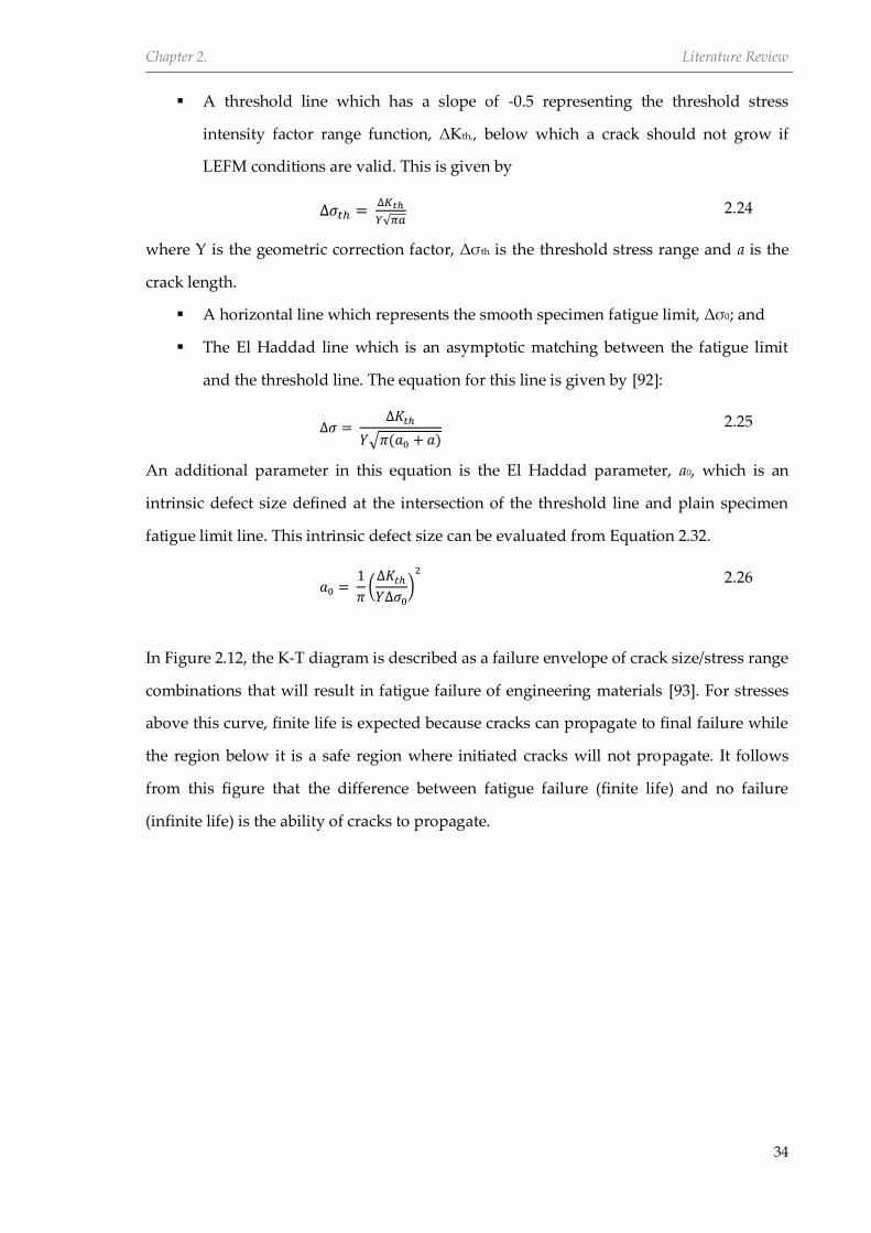
A threshold line which has a slope of -0.5 representing the threshold stress
intensity factor range function, ΔKth,, below which a crack should not grow if
LEFM conditions are valid. This is given by
∆𝜎𝑡ℎ = ∆𝐾𝑡ℎ
𝑌√𝜋𝑎 2.24
where Y is the geometric correction factor, Δσth is the threshold stress range and a is the
crack length.
A horizontal line which represents the smooth specimen fatigue limit, Δσ0; and
The El Haddad line which is an asymptotic matching between the fatigue limit
and the threshold line. The equation for this line is given by [92]:
∆𝜎 = ∆𝐾𝑡ℎ
𝑌√𝜋(𝑎0 + 𝑎) 2.25
An additional parameter in this equation is the El Haddad parameter, a0, which is an
intrinsic defect size defined at the intersection of the threshold line and plain specimen
fatigue limit line. This intrinsic defect size can be evaluated from Equation 2.32.
𝑎0 =
1
𝜋(
∆𝐾𝑡ℎ
𝑌∆𝜎0
)2
2.26
In Figure 2.12, the K-T diagram is described as a failure envelope of crack size/stress range
combinations that will result in fatigue failure of engineering materials [93]. For stresses
above this curve, finite life is expected because cracks can propagate to final failure while
the region below it is a safe region where initiated cracks will not propagate. It follows
from this figure that the difference between fatigue failure (finite life) and no failure
(infinite life) is the ability of cracks to propagate.

Chapter 2. Literature Review
35
Figure 2.12 Schematic showing the Kitagawa-Takahashi diagram and the limiting conditions for
fatigue failure [93].
Figure 2.13 Schematic showing the relationship between the limiting threshold stress and crack
size and the short crack growth and long crack growth regimes of the Kitagawa-Takahashi
diagram [94].
Figure 2.13 describes the K-T diagram based on different types and regimes of crack
growth. These include the microstructurally short crack, physically short crack and long
crack regimes [94]. In the microstructurally short crack regime, where the crack length is
typically of the order of microstructural dimensions, there is an influence of the
microstructure on whether cracks will be arrested or continue to propagate [33, 58, 95]. As
shown in the diagram, a crack with length less than the strongest microstructural barrier
(microstructural threshold), which is at a given distance d, will result in no failure with
respect to the plain fatigue limit, Δσ0. Also, cracks with lengths d1 and d2, shorter than the
Non-propagating cracks

Chapter 2. Literature Review
36
size of the strongest microstructural barrier, d, will be arrested (non-propagating cracks) if
the applied stress range is smaller than the plain fatigue limit [95]. In the long crack
growth regime, the threshold stress intensity factor range defines a limiting condition for
long crack propagation and is independent of crack size for crack lengths greater than a
limiting crack length, l (mechanical threshold). However, above this threshold length, the
stress range required to achieve the limiting stress intensity factor (threshold stress range)
decreases with increase in crack size [37, 69, 95]. This implies that for a given size of long
crack that is greater than the threshold length, crack growth will occur if the applied
stress range is greater than the threshold stress range [95]. The regime between that of
microstructurally short cracks and long cracks represents the physically short cracks and
is the transition between the microstructural, d, and mechanical, l thresholds. In this
region, below the mechanical threshold, the curve deviates from the threshold stress
intensity range line thus indicating that the threshold stress intensity factor for this crack
regime cannot be predicted using LEFM analysis. The curve also approaches the plain
fatigue limit at the microstructural threshold. The physically short crack region is
important because if the defect size is greater than the mechanical threshold, LEFM is
applicable for explaining crack propagation. The ability of the K-T diagram to successfully
define the combination of crack size (microstructural and mechanical thresholds) and
stress range that will lead to failure has given rise to various generalized diagrams, which
can be used for design and residual life assessment purposes. These diagrams, which are
usually in the form of fatigue damage maps, have been generated for different materials
and also applied for fatigue assessments. Venkateswaran et al. [96] generated stress versus
crack length plots at different stress ratios for a ferritic steel weld metal, based on the K-T
diagram. From the generated plots, the limiting stress range required to achieve a desired
fatigue life for the components made from the steel and containing different crack sizes
was determined. Peters et al. [97] examined the effect of applied and residual stresses due
to foreign-object damage and stress ratio on high cycle fatigue failures in a titanium alloy.
In their study, a modified K-T diagram, which describes the limiting conditions for high
cycle fatigue failure, was presented. Various generalised diagrams have also been
proposed for design purposes [98-101].
Chapter 2. Literature Review
37
2.7 Environment Assisted Fatigue
It is generally accepted that the effect of the interaction between the environmental time-
dependent electrochemical processes (corrosion) and applied stress can lead to a
significant reduction in the design life of engineering structures and components. For
instance, materials with good corrosion resistance in the absence of applied stress and
those with superior fatigue strength in air, can exhibit poor behaviour under the conjoint
action of stress and corrosion [102]. Environment assisted cracking (EAC) can generally be
classified into three forms [103]:
Stress corrosion cracking (SCC)
Hydrogen-assisted cracking (HAC)
Corrosion fatigue (CF).
2.7.1 Hydrogen-assisted Cracking (HAC)
HAC involves the diffusion of and build-up of hydrogen in the metal when exposed to
hydrogen-rich environments thus, assisting the initiation and propagation of cracks. This
could be through reduction of surface energy by hydrogen adsorption, reduction in the
inter-atomic bond strength or hydrogen molecules exerting pressure against the wall of
the crack. Effects of hydrogen damage include hydrogen embrittlement, loss of tensile
strength, blistering, hydride formation, micro-perforation and degradation in flow
properties. HAC may also contribute to the failure of materials by SCC and CF. For
instance, in some metal-environment systems under cathodic protection, SCC has been
found to result from hydrogen-induced subcritical crack growth [104].
2.7.2 Stress Corrosion Cracking (SCC)
SCC occurs when a metal is simultaneously subjected to a static stress of sufficient
magnitude and a corrosive environment [105]. Usually, a specific environment and
metallurgical condition, in terms of the composition and structure of the alloy is also a
requirement. For example, the SCC of copper alloys is usually due to the presence of
ammonia in the environment while for stainless steels and aluminium, the presence of
chloride ions is the main cause [106, 107]. In SCC, crack propagates within the material
through the internal structure usually living the outer surface unarmed. Different
mechanisms have been proposed to explain the interaction between stress and corrosion

Chapter 2. Literature Review
38
at the crack tip during SCC damage. They include active path intergranular cracking
[108], film rupture/anodic dissolution [109], and adsorption-related mechanisms [106,
110]. In SCC, the threshold SIF below which cracks will not propagate, 𝐾𝐼𝑠𝑐𝑐:, is typically
below the threshold SIF implying that cracking can occur at far lower SIF values than
when there is no corrosion. SCC is influenced by factors such as material (microstructure,
composition, grain size) [111], mechanical (stress, strain rate) [112],and environment
(temperature, pH, solute concentration, solute species) [113].
2.7.3 Corrosion Fatigue
Historically, corrosion fatigue damage has been recognized as a major cause of failure of
engineering structures hence, it is a major concern for design engineers. CF is a material
degradation process involving the synergistic damage actions of an aggressive
environment and mechanical cyclic loading [114-116]. Generally, the effect of this synergy
on the damage process is more severe than the sum of their individual effects when acting
separately i.e. corrosion or fatigue [31, 102]. Investigations on the fatigue behaviour of
these structures in aggressive environments revealed significant reduction in fatigue
strength in these environments far below that observed in air. In some cases, the fatigue
limit is completely eliminated. Under CF conditions, no matter how low the stress
amplitude is, fracture can eventually occur in the engineering structure [117-120]. This is
in contrast to fatigue in air where crack can nucleate but do not grow (crack arrest) at
stress levels below the fatigue limit. A thorough understanding of the stages of corrosion
fatigue and associated mechanisms is essential in order to optimise design and maximise
the lifetime of structures operating in aggressive environments.
The influence of the environment can be related to the crack initiation and crack growth
processes especially in the early stages of corrosion fatigue damage. In the initiation stage,
the environment can accelerate the nucleation of cracks by creating localised defects such
as corrosion pits. Corrosion pits can act as stress intensifiers and also provide a pit
chemistry that is favourable for crack nucleation [121-124]. After the nucleation of cracks,
the environment can influence crack growth rate through strain-assisted anodic
dissolution. Here, the environment can influence Stage I crack growth by overcoming the
microstructural barriers that retard crack growth or lead to crack arrest. Furthermore, it
can lead to reduction in the Stage I to Stage II transition crack length [36, 88, 89]. A

Chapter 2. Literature Review
39
schematic of the influence of environment on defect size at different stages of fatigue
damage in comparison with that of air is shown in Figure 2.14. The figure highlights a
reduction in the number of cycles at stage I-to-Stage II transition size in the environment.
The environment usually accelerates crack growth rates through anodic dissolution but in
some cases, crack growth rates may be reduced through crack tip blunting and corrosion
product-induced crack closure [122]. Akid [88, 125, 126] reported that the major effect of
the environment is in the early stages of corrosion fatigue crack growth when crack size is
below a critical value. When the crack size is greater than this value, the damage process
is dominated by mechanical factors and the environment has less effect. Consequently,
the air and corrosion fatigue crack growth rates merge since the growth rate is now
controlled by the stress intensity at the crack tip with limited contribution from
environment-assisted growth.
Figure 2.14 Schematic of defect development stages in air and aggressive environment [127].
Results from studies [123, 127, 128] on systems where pits are precursors to cracking have
led to the conclusion that corrosion fatigue can be considered as a multi-stage damage
accumulation process consisting of the following stages: surfaces include surface film
breakdown, pit development, pit-to-crack transition, short crack growth and long crack
growth.

Chapter 2. Literature Review
40
2.7.4 Corrosion Fatigue Mechanisms
The rate of crack growth in CF is governed by the interaction between the chemical and
mechanical mechanisms occurring at the crack tip [103, 129]. CF is such a complex process
that no one mechanism can describe all cases. Generally, the mechanisms that contribute
to CF crack advancement are stress-assisted dissolution (slip dissolution) [110, 130],
corrosion-product-induced crack closure [131] and hydrogen-induced cracking [132, 133]
or combination of any [53, 103, 129, 134, 135].
2.7.4.1 Anodic Dissolution Mechanism
In fatigue cracking, it is known that the crack tip becomes anodic relative to the rest of the
material surface. In this model, the protective film is ruptured either by the applied stress
or halide attack near the crack tip. The exposed base metal is then attacked by the
corrosive media causing dissolution and consequently sharpening of the crack tip
depending on the rate of re-passivation. The re-passivation reaction competes with the
dissolution reaction, and when the rate of the former exceeds that of the latter, the passive
film is repaired and the anodic dissolution process stops. The crack growth rate is
dependent on the rate of anodic dissolution and rate of re-passivation amongst others
[103, 135]. The process then begins all over again with the rupture of the passive film
thereby exposing the metal at the crack tip to the corrosive media. A schematic illustration
of stress-assisted dissolution mechanism is shown in Figure 2.15. Ford [130] verified the
slip dissolution and hydrogen embrittlement mechanisms in Al-Mg alloy and concluded
that crack growth was controlled by slip dissolution. The environment may also
decelerate crack growth rates. This can occur in two ways. The increase of width of cracks
by anodic dissolution effectively decreases the stress intensity factor thereby resulting in
lower SIF available for crack extension. The second is oxide-induced crack closure, where
the corrosion products cause a wedge effect thereby decrease the effective SIF range.
Figure 2.16 shows a schematic of the wedge effect mechanism induced by corrosion
products.

Chapter 2. Literature Review
41
Figure 2.15 Schematic illustration of stress-assisted dissolution mechanism [136].
Figure 2.16 Schematic illustration of the wedge effect mechanism induced by corrosion products
[136].
2.7.4.2 Hydrogen-induced Mechanism
The presence of hydrogen at the crack tip can aid the propagation of cracks under cyclic
loading thereby accelerating the crack growth rate [129]. Gaseous hydrogen environments
can aid in crack growth as the relatively high pressure from diatomic hydrogen gas act as
a localized force in the crack region supplementing the stress on the metal and
consequently accelerate the crack growth rate. Cathodic reactions associated with the
corrosion of the metal release hydrogen ions that combine to form gaseous hydrogen (H2)
within the metal lattice, which results in a pressure build-up in the crack void space [103].
Atomic hydrogen dissolved in a metal can also lead to an increased crack growth rates.
Hydrogen atoms within a metallic crystalline structure can lower the bond strength
between the individual atoms [137, 138]. Moreover, hydrogen atoms generated during the
corrosion process can diffuse through a metallic structure under an applied stress, and
collect near the point of maximum stress [135]. The consequence of dissolved hydrogen in
a metal is that it can reduce the strength of the metal, and if a crack exists, it will

Chapter 2. Literature Review
42
propagate with less resistance where there is a concentration of hydrogen atoms [103,
135]. Adsorbed hydrogen lowers the surface energy of the metal, which facilitates crack
growth. Figure 2.17 shows a schematic of the hydrogen-induced mechanism. In an
electrolyte, the critical steps involve the diffusion of water molecules and hydrogen ions
between the crack walls and the crack tip; production of adsorbable hydrogen atoms at
the crack tip; and diffusion to and adsorption of the hydrogen atoms at preferential
locations ahead of the crack tip [31]. The preferential locations can be grain boundaries or
regions of high stress triaxiality. In situations involving the formation of a passive oxide
film on the freshly created surface, the reaction at the crack tip which influences
dissolution, hydrogen ion reduction, or crack growth is controlled (at a given
electrochemical potential) by three factors: the oxide rupture rate, the solution renewal
rate to the crack tip, and the re-passivation rate [31].
Figure 2.17 Schematic illustration of hydrogen embrittlement mechanism [136].
2.7.5 Corrosion Fatigue Stages
When pits are precursors to corrosion fatigue cracking, the fundamental stages in the
overall crack development process includes surface film breakdown leading to pit
initiation, pit growth, pit-to-crack transition, short crack growth and long crack growth
[139]. These stages are shown schematically in Figure 2.18. A reliable prediction of the
complete corrosion fatigue process in engineering components would require a
quantitative understanding of each stage.

Chapter 2. Literature Review
43
Figure 2.18 Schematic showing the behaviour of fatigue cracks under and corrosion fatigue
conditions [119].
2.7.5.1 Surface Film Breakdown
Most engineering metals and alloy, with the exception of the noble metals, develop, to
some degree, a passive film on the surface as a result of oxidation in air. Depending on
alloy composition, temperature, environment, potential, magnitude of applied stress and
exposure history, this film can vary in structure, composition, electronic conduction,
porosity thickness and protectiveness [140]. These properties of the surface film determine
the inherent resistance of a material to electrochemical damage. The most important
criterion for pitting is the pitting potential below which pitting does not occur and above
which pits nucleate and develop [141]. However, in some type of systems such as mild
steel in chloride-containing solution, no pitting potential is observed. Most metal surfaces
have physical or chemical inhomogeneities that can be more susceptible to attack and
hence, become the favourable sites for pit initiation.
Preferential attack is due to the difference in the properties of the passive film at these
sites from that of other parts of the metal matrix [139]. In steels, these inhomogeneities
include sulphide inclusions, oxide inclusions, second phase precipitates, grain
boundaries, exit points of dislocations and mechanical flaws [142-144]. During pit
initiation, in the presence of depassivating agents like chloride ions, this passive film
breaks down and allows the environment to be in contact with metal surface thereby
allowing active dissolution of the exposed surface (pitting). Mechanisms of passive film

Chapter 2. Literature Review
44
breakdown and pit initiation can be classified into three: passive film penetration [145],
passive film breaking [146] and adsorption [147].
2.7.5.2 Pit Growth
The breakdown of the surface film leads to dissolution (pitting) of the underlying bulk
metal. Pit growth is a time-dependent process that involves two stages: metastable pitting
and pit growth. Metastable pits are pits, which initiate and grow for a limited period of
time before repassivating. Metastable pits have been reported for stainless steel [148-151],
mild steel [152] and aluminium [153, 154]. Pits that survive the metastable stage are
referred to as stable pits and they will continue to grow under favourable environmental
conditions. Frankel [140] and Szklarska [141] both considered pitting to be autocatalytic in
nature; once a pit starts to grow, the conditions developed are such that further pit
growth is promoted. Due to the time-dependent nature of metal dissolution, pit sizes are
also generally time-dependent [155, 156]. Pit growth can be controlled by the same factors
that can limit any electrochemical reaction namely charge transfer (activation), ohmic
effects, mass transport or combination of these factors. The rate of pit growth depends on
several factors including potential [141, 157], temperature [17, 158], chloride ion
concentration [159, 160], alloy effects [161, 162], applied stress [118, 143] and inhibition
[163].
2.7.5.3 Pit-to-crack Transition
The pit-to-crack transition stage is an important stage of the CF process. After initiation,
corrosion pits grow under the influence of cyclic stress and create conditions which
facilitate cracking. These conditions are generally related to local electrochemical and
mechanical factors. When prevailing conditions are favourable, cracks will initiate from
the pits. To model the CF process accurately, it is important to consider this stage.
2.7.5.4 Corrosion Fatigue Cracking
The crack growth stage starts when cracks have initiated from pits. During this stage, the
environment can have varying influence on the growth behaviour.
2.7.5.5 Corrosion Fatigue Long Cracks
As in-air tests, the growth of corrosion fatigue cracks can be characterised using the LEFM
approach but in a simulated operating environment. The propagation rates of long cracks

Chapter 2. Literature Review
45
can be greater than in air. A number of relationships between crack growth rates and
stress intensity factor have been observed in different metal-environment systems. These
may be broadly classified by three patterns of behaviour [31, 164].
True corrosion fatigue (Figure 2.19a) – this type of behaviour is often observed in
materials which are resistant to stress corrosion cracking, thus characterises the
synergistic effects of cyclic loads and aggressive environment. Features of this
type of behaviour are the lower threshold SIF range and increase rate of crack
growth compared to in air. Thus it is possible to predict the extent to which crack
growth is affected by the environment.
Stress corrosion fatigue (Figure 2.19b) – this is typical of where there is a
substantial environment-enhanced sustained-load crack growth component.
Because the effects of stress corrosion and fatigue are additive and can be
superimposed, it is possible to predict corrosion fatigue behaviour when stress
corrosion data in the same environment and fatigue data in air are available.
Above the threshold KISCC for stress corrosion cracking, environment effects are
significant but are negligible below this level.
Combined behaviour (Figure 2.19c) – a complex combination of true corrosion
fatigue and stress corrosion fatigue may also be obtained.
Figure 2.19 Schematic of three types of corrosion fatigue crack growth behaviour (a) true corrosion
fatigue (b) Stress corrosion fatigue (c) combined behaviour [164].
(a) (b) (c)

Chapter 2. Literature Review
46
Corrosion Fatigue Short Cracks
Under corrosion fatigue conditions, the aggressive environment can have significant
effect on the propagation rate of short cracks. Corrosion tends to weaken the resistance of
microstructural barriers such as grain and phase boundaries through metal dissolution
and crack tip expansion and thus enable cracks to re-initiate in the adjacent grains. At
later stages, the effect of corrosion is somewhat hidden by the mechanical driving force,
which would have increased due to crack length increase and therefore, becomes the
controlling parameter. Previous studies have reported higher propagation rates than long
cracks under the same stress intensity factor range [131, 132, 165]. A typical behaviour of
short fatigue cracks under corrosion fatigue conditions was reported by Akid [166] where
crack growth rate in the presence of the environment was plotted as a ratio to that in air
(Figure 2.20). Not only were crack growth rates observed to be retarded by
microstructural features, in this case prior austenite grain boundaries, they were
significantly higher than in air. In addition, the important effect of the environment is
highlighted whereby the ratio increases when the crack approaches a barrier to its growth
and subsequently decreases after crossing the barrier. Previous investigations by Akid
and co-workers [36, 53, 88-90, 125, 126, 128, 166] can be summarised as follows:
aggressive environment influences short fatigue crack growth depending on stress
level and crack size,
microstructural features such as the grain boundaries can cause partial retardation
of propagation of short cracks but growth rates still remain higher than in air,
the influence of microstructure is significant in the short crack growth regime but
less in the long crack regime,
aggressive environment, through strain-assisted dissolution, can eliminate the
microstructural barriers and allow re-propagation of non-propagating cracks, and
strain-assisted anodic dissolution reduces the critical length for Stage I to Stage II
transition thereby reducing the physically small crack regime compared to air
fatigue. The transition crack length can be as low as one to two units of
microstructural dimensions.

Chapter 2. Literature Review
47
Figure 2.20 Ratio of fatigue crack growth rate in 3.5 % NaCl to fatigue crack growth rate in air as
a function of surface crack length [166].
Gangloff [133] reported that the growth of short fatigue cracks in aqueous environments
was faster than long cracks. Piascik and Williard [167] and Tanaka et al. [165, 168]
investigated the growth characteristics of short cracks and reported that the test
environment accelerated the growth rates of short cracks faster than in air. Kondo [169]
also observed in two low alloy steels that short cracks from pits propagated at ΔK values
well below the ΔKth for a long crack for these materials. Corrosion can also influence short
crack growth through oxide-induced crack closure. Suresh et al. [170] reported that at low
stress ratios, near-threshold short crack growth rates were significantly reduced in
aqueous compared to dry environments due to the formation of corrosion deposits on the
crack surfaces, which enhanced crack closure. Gangloff and co-workers suggested that the
higher growth rates of short cracks was due to differences in the local crack tip
environment, which is a consequence of the differences in the electrochemically active
surface-to-volume ratios, which is due to crack size [67, 132, 133, 171]. In a recent review,
Turnbull [172] discussed different electrochemical mechanisms that may determine the
effect of the environment on corrosion fatigue short crack growth. These factors include:
mass transport of reactive species into and out of cracks through pumping action
of opening and closing of cracks due to cyclic loading
changes in crack tip potential which may result from potential drop in the crack
(between the crack tip and crack mouth) and outside the crack (between the crack
mouth and the metal surface away from the crack), both of which affect the extent

Chapter 2. Literature Review
48
crack tip polarisation, and the effect of bulk flow whereby mixing of crack
and bulk solutions can prevent the development of solution chemistry that
propmotes crack growth.
2.7.5.6 Factors affecting corrosion fatigue crack growth
Several variables can influence corrosion fatigue behaviour of metals and alloys. These
may be divided into three main groups: mechanical, metallurgical and environmental.
Metallurgical factors – These include alloy composition [140], distribution of
alloying elements and impurities [140, 173], microstructure [89, 174], welding
defects [116] and heat treatment [175].
Environmental factors – Because corrosion fatigue is a damage process involving
an aggressive environment, factors that influence the concentration of damaging
species will affect the process. These include concentration of damaging species
[176], electrochemical potential [177], pH [177], temperature[178, 179] and
inhibitors [180-182].
Mechanical factors – As corrosion fatigue involves cyclic loading, variables that
influence the loading spectrum will affect corrosion fatigue behaviour. These
include stress range [118, 183, 184], cycle frequency [122, 174, 179, 185], stress ratio
[9, 186], load waveform [134], and residual stresses [187].
2.8 Crack Nucleation from Corrosion Pits
Although corrosion fatigue cracks can initiate from features such as inclusions and grain
boundaries, corrosion pits are generally the preferred sites for crack nucleation in metal-
environment systems where pits are precursors to cracking [9, 16, 117, 121, 123, 167, 169,
188-199]. Figure 2.21 shows an example of the transition from pitting to cracking in
turbine blade steel in chloride environment. The transition represents a stage when
damage transitions from that of a time-dependent corrosion phenomenon to that of a
mechanical cycles-dependent phenomenon [139, 200]. From current understanding, the
growth of corrosion pits under cyclic loading is thought to create conditions, which
facilitate crack nucleation. These conditions are generally thought to be a complex
combination of metallurgical, electrochemical, mechanical and in-service factors [105].

Chapter 2. Literature Review
49
Generally, models for crack initiation in aqueous environment have been based on the
following events:
1. preferential attack at sites where the protective film on the surface of an alloy
under cyclic load has been ruptured.
2. stress concentration at the roots of corrosion pits thus making them crack
nucleation sites.
3. preferential dissolution at regions where plastic deformation is localised, with the
less deformed surrounding regions acting as cathodes.
4. reduction in surface energy of the metal due to the adsorption of environmental
species such as hydrogen.
Figure 2.21 Typical pit-to-crack transition observed on pre-pitted specimen in corrosion fatigue (a)
pit before and (b) after transition [9].
From a mechanical perspective, the presence of geometric discontinuities interrupt the
stress pattern in engineering components and tend to make it non-uniform, and
consequently resulting in an increase in local stress level around the discontinuities.
Hence, corrosion pits can lead to localisation of stress and strain [1, 121, 201-204]. The
magnitude of the increase in local stress and strain can be determined using the
theoretical elastic concentration factor, defined as the ratio of maximum local stress to the
nominal stress. The nominal stress is taken as a reference stress value and is dependent on
geometry of specimen and load type while the local stress is dependent on the geometry

Chapter 2. Literature Review
50
of the discontinuity and applied stress. The stress concentration factor depends only on
the geometry of the discontinuity. It is worthy of note that the stress concentration factor
is an elastic parameter and therefore can only be used as an approximation of the
prevailing stress and strain around the pit. In reality, components containing pits may be
subjected to elastic-plastic conditions depending on pit size and applied stress. In contrast
to elastic conditions where applied stress and strain a linearly related and stresses can
reach unrealistic values, stresses typically do not increase beyond the yield limit of the
material when plastic conditions are employed. This can result in a redistribution of
stresses and strains around a pit and therefore has implications when conducting
mechanics based studies on understanding how corrosion pits facilitate crack nucleation.
For instance, whereas purely plastic analysis of stress and strain around pits showed
similar stress and strain patterns, which is concentrated at the pit bottom, elastic-plastic
analysis of the same pits showed that increase in plastic deformation with increasing
stress resulted in redistribution of stresses and localisation of strain towards the pit mouth
[121, 202]. This also undermines current pit-to-crack transition models, which are based
on the ∆𝐾𝑡ℎ , a parameter that is based small-scale yielding.
Ahn [122] observed a dependence between fatigue limit and pit depth, but only at pit
depths above 150 µm. They also reported a decrease in the number of cycles required to
initiate a surface crack with increasing pit depth and increasing applied stress range. In-
air tests only provide information on the mechanical effect of pits on fatigue life. The
influence of corrosion on fatigue life requires the presence of an aggressive environment.
Anh [122] observed a further reduction in the number of cycles to initiate a crack in 1M
NaCl solution compared to those in air. For the HSLA steel tested, the crack initiation life
in air varied between 65% to 94% compared to 35% to 75%, in the chloride environment.
They concluded that the presence of the environment changed the fatigue behaviour from
being initiation-dominant to propagation-dominant. Pao [205] investigated the influence
of corrosion pits on the fatigue strength of an aluminium alloy and reported that both the
threshold stress intensity and fatigue crack initiation life of polished specimens in air were
reduced by half when pre-existing corrosion pits were present. Wang [206] reported that
the presence of pre-existing corrosion pits produced by immersion in 3.5% NaCl, over
different exposure times, accelerated crack nucleation stage and consequently reducing
fatigue life by up to a factor of 100, compared to smooth specimens. Jones and Hoeppner

Chapter 2. Literature Review
51
[156] investigated the transition of corrosion pits to cracks during corrosion fatigue in
aluminium alloys. They observed that the crack nucleation stage accounted for a large
fraction of the fatigue life. They also reported that pit surface area, pit geometry,
proximity to other surrounding pits and pit depth are quantities which play an important
role in determining when a crack will nucleate from a pit.
There is experimental and in-service evidence indicating that multiple corrosion pits can
initiate and develop close to each other on engineering components [121, 207]. Multiple
pits can coalesce and form larger pits, while the stress fields around those pits that do not
coalesce can interact to influence crack nucleation, leading to crack coalescing into a single
crack [156, 207]. Horner et al. [121] also observed development of multiple pits in high
strength disc steel in a chloride environment. Their observation identified coalescence of
cracks that initiated from adjacent pits as the key factor in crack propagation behaviour.
Although the nucleation of cracks from pits has been correlated with strain localisation,
the location around a pit where a crack will preferably initiate still remains unclear. In
some systems, cracks have been observed to nucleate at the bottom of pits [195, 207, 208]
while in others crack initiation was observed at the pit mouth [9, 121, 202, 209]. From their
tests on stainless steel containing artificial corrosion pits, Masaki [195] observed fatigue
cracks initiated at the bottom of the pits even at nominal stress amplitudes below plain
specimen fatigue limit. The phenomenon of initiation of cracks at the pit bottom was
explained on the basis of the differences in crack initiation stress of the material at the
bottom of the pit compared to the pit mouth. Initiation is favoured at a point where the
local stress is larger than the crack initiation stress of the material (assumed to be equal to
the fatigue strength of an electrochemically polished plain specimen). In Figure 2.22, the
favourable points are Points A and C. However, because the specimens were
mechanically polished, the surface layer will be work-hardened thereby resulting in
increase in the crack initiation stress compared to the bottom. Hence, cracking is favoured
at the pit bottom. Using X-Tay tomography, Turnbull and co-workers [105, 121, 202]
observed crack nucleation at the mouth of pits in high strength steel in corrosion fatigue
(Figure 2.23).

Chapter 2. Literature Review
52
Figure 2.22 Fatigue crack initiation model [195].
Figure 2.23 Example of crack emerging from the pit mouth as observed by X-ray tomography. The
image is best considered as being viewed from inside the steel [202].
2.9 Corrosion Fatigue Lifetime Modelling
There are established methodologies and industry standards for predicting the fatigue life
of engineering structures in air (e.g. R6 [164] and BS 7910 [210]) all of which are based
upon the application of the Paris law, and its various modifications, derived from data
generated from pre-cracked specimens. Likewise, under corrosion fatigue conditions, a
similar approach is employed, although tests are carried out in a simulated aggressive
environment. Since CF is a synergistic process involving mechanical fatigue and
aggressive environment, several models have been proposed to describe the effect of the
latter on fatigue. A brief review of these models is discussed below.
Pit bottom
Short crack initiating
from pit mouth

Chapter 2. Literature Review
53
2.9.1 The Superposition Model
A superposition model was first used to describe corrosion fatigue crack propagation by
Wei and co-workers [211, 212] who considered the total corrosion fatigue crack growth
rate to be the superposition of a plasticity-driven crack extension component with a
second component representing the interaction between plastic deformation and chemical
reactions.
(𝑑𝑎
𝑑𝑁)
𝑒= (
𝑑𝑎
𝑑𝑁)
𝑚 + (
𝑑𝑎
𝑑𝑁)
𝑐𝑓 2.27
where (da/dN)e is the crack growth rate in aggressive environment, (da/dN)m is the rate of
plasticity-driven fatigue crack propagation in an inert environment and (da/dN)cf is the
difference between the total growth rate and ‘pure’ fatigue growth rate representing the
effect of interaction between chemical reactions and plastic deformation.
2.9.2 The Competition Model
In this model [213], corrosion fatigue crack propagation is considered as a competition
between mechanical fatigue and cycle-time dependent corrosion fatigue. The measured
corrosion fatigue growth rate is taken as the fastest (dominant) process.
(da
dN)
e= (
da
dN)
m(θ) + (
da
dN)
cf (∅) 2.28
where θ = 1 - φ (both measured by fractographic analysis).
In an environment dominant cracking process, φ = 1 and the (da/dN)m << (da/dN)cf.
Therefore,
(𝑑𝑎
𝑑𝑁)
𝑒= (
𝑑𝑎
𝑑𝑁)
𝑐𝑓 2.29
2.9.3 Modified Short Crack Growth Model
The Hobson-Brown and Navarro-de les Rios models, previously discussed, were
modified by Akid and Miller [125, 126] to account for environmental effects on both short
and long cracks. In this model, corrosion fatigue crack growth rate incorporates the
summation of crack growth rate in air (representing the mechanical driving force) and
growth rate as a result of dissolution in the environment (representing the chemical
driving force based on anodic dissolution current).

Chapter 2. Literature Review
54
(𝑑𝑎
𝑑𝑁)
𝑒𝑛𝑣= (
𝑑𝑎
𝑑𝑁)
𝑎𝑖𝑟 + (
𝑑𝑎
𝑑𝑁)
𝑑𝑖𝑠𝑠 2.30
(𝑑𝑎
𝑑𝑁)
𝑑𝑖𝑠𝑠= (
𝑀𝑖𝑎
𝑍𝐹𝜌)
1
𝑤 2.31
where M is the atomic weight of the corroding metal, ia is the anodic dissolution current,
Z is the valency, F is the Faraday's constant, ρ is density and w is the cyclic frequency.
2.9.4 Pitting Corrosion Fatigue Models
In material-environment systems where pitting is a precursor to cracking, CF lifetime
prediction is a complex procedure because of the need to account for pit initiation, pit
growth, crack initiation, short crack growth and long crack growth. Current models
proposed to address this [124, 169, 188, 214-217] are based on two-stage process involving
pit growth and long crack growth. The pit growth stage is modelled using the pit growth
theory while the crack growth is modelled using conventional da/dN–ΔK test data. The
point of transition is defined by the threshold SIF range. These models are summarised
below.
2.9.4.1 Hoeppner Model
This mechanistic model [216] was proposed for predicting the critical pit depth to
nucleate a crack under pitting corrosion fatigue conditions. The pit size at a given stress
condition at which a Mode I crack develops was determined from the fatigue crack
growth threshold. The number of cycles required to generate a pit large enough to
develop a Mode I crack, i.e. the time taken to attain the pit depth that satisfies the
threshold condition was determined using pit growth theory while the number of cycles
to propagate the crack to fracture was then determined using SIF range. The total life is
then given by a summation of the two. The model is given by:
𝐾 = 1.1𝜎√𝜋 (𝑎
𝑄) 2.32
𝑑 = 𝐶𝑡3 2.33
where K, σ, a, Q, t, d and C are stress intensity factor, applied stress, pit length, a function
based on crack shape, time taken to attain pit depth for corresponding threshold value, pit
depth and constant dependent upon material and environment respectively.

Chapter 2. Literature Review
55
2.9.4.2 Lindely Model
Lindely et al. [214] proposed a model for determining the threshold stress intensity factor
at which a crack would initiate from a pit by considering corrosion pits as semi-elliptical
sharp cracks. The model was given as:
𝐾𝑡ℎ = ∆𝜎√(𝜋𝑎) [1.13 − 0.07 (
𝑎𝑐)
0.5]
[1 + 1.47 (𝑎𝑐
)1.64
]0.5
2.34
where ΔKth, a and c and Δσ are threshold stress intensity factor, minor axis of semi-
elliptical crack, major axis of semi-elliptical crack and applied stress range respectively.
2.9.4.3 Kawai and Kasai Model
In this model [215], LEFM approach was employed to determine the critical depth from a
fatigue crack would grow by estimating the allowable stress intensity threshold under
corrosion fatigue conditions. The model, which considered corrosion pits as elliptical
cracks, is given as
∆𝐾𝑎𝑙𝑙 = ∆𝜎𝑎𝑙𝑙√𝜋ℎ𝑚𝑎𝑥 2.35
where ΔKall, Δσall, F and hmax are allowable stress intensity threshold, allowable stress range,
geometric factor and maximum pit depth respectively.
2.9.4.4 Kondo Model
Kondo [169] proposed a model by estimating the critical pit condition using both stress
intensity and pit growth relations. The model considered corrosion pits as sharp
hemispherical cracks and proposed that the critical condition for transition is that crack
growth rate must exceed pit growth rate. The model was given as:
∆𝐾𝑝 = 2.24𝜎𝑎√𝜋𝑐
𝛼
𝑄
2.36
𝑐 = 𝐶𝑝𝑡1/3 = 𝐶𝑝(𝑁/𝑓)1/3
2.37
where σa, Q, c, t, N and f represent the stress amplitude, pit aspect ratio, shape factor, pit
radius, number of fatigue cycles and cyclic frequency respectively.

Chapter 2. Literature Review
56
2.9.4.5 Chen Model
Chen et al. [188] proposed a model for predicting crack initiation based on concepts of
fatigue crack growth thresholds and a competing pitting/cracking rate. The transition
criteria from pitting to cracking was proposed as (i) the equivalent stress intensity factor
range must be greater than ∆𝐾𝑡ℎ for long crack growth and (ii) the fatigue crack growth
rate must exceed the pit growth rate. The transition SIF, ∆𝐾𝑡𝑟, crack growth rate and pit
growth rate were given by
∆𝐾𝑡𝑟 =
1.12𝐾𝑡∆𝜎√𝜋𝐶𝑡𝑟
𝛷
2.38
(𝑑𝑎
𝑑𝑁)
𝑝𝑖𝑡=
𝐶𝑝
2𝜋∙ 𝛽2𝑐−2 2.39
(𝑑𝑎
𝑑𝑁)
𝑐𝑟𝑎𝑐𝑘= 𝐶𝐹(𝑘𝑡∆𝜎)𝑛𝛷−𝑛𝑐0.5𝑛𝑓 2.40
where ∆𝐾𝑡𝑟 is SIF for transition, 𝐾𝑡 is elastic stress concentration factor, c is half-pit
diameter, Δσ is applied stress range, Φ is shape factor determined by the pit diameter, β
is pit aspect ratio, f is cyclic frequency, and 𝐶𝐹 , 𝐶𝑝 and n are constants.
2.9.5 Multi-stage Modelling
CF lifetime prediction is a complex procedure because of the need to account for pit
initiation, pit growth, crack initiation, short crack growth and long crack growth. Hence,
the pitting corrosion fatigue models enumerated above are simplified into a two-stage
process consisting of pit growth and long crack growth. The criteria for transitioning from
a pitting to cracking is also defined phenomenologically in that the threshold SIF
associated with a pit must exceed that of the pit and the crack growth rate is greater than
the pit growth rate. Following initiation, the crack is considered to behave as a long
fatigue crack hence crack growth rates can be predicted based on LEFM. Whilst
correlations between model predictions and experiments have been made, a major
concern surrounds the underlying assumptions of these models.
In the pitting corrosion fatigue models, corrosion pits are considered to be effective
cracks, thereby allowing the calculation of a SIF range using LEFM concepts. Therefore,
the threshold SIF is assumed to control the transition of pits to cracks. It is considered that
cracks will not initiate or propagate when the pit depth is lower than a threshold depth.
However, the questions are whether corrosion pits are truly effective cracks and whether

Chapter 2. Literature Review
57
cracks will initiate from pits with depths less than the threshold pit depth. Other concerns
are whether the use of a fracture mechanics parameter, ∆𝐾𝑡ℎ, which is obtained from pre-
cracked specimens is applicable to pits growing on smooth specimens or components.
From the point of view of LEFM, corrosion pits may also induce significant local plasticity
hence, resulting in a breakdown of small-scale yielding condition required for LEFM
analysis. Moreover, the conditions governing pit-to-crack transition will most likely
depend on both mechanical and electrochemical factors rather than the LEFM threshold
fracture parameter presumed in these models. It is also assumed implicitly that, at the
point of crack-pit transition, cracks must have the same depth as the nucleating pit and
that crack initiation will occur at the bottom of a pit. However, recent studies have shown
that cracks can initiate from pit mouth and can have depths that are far smaller than that
of the pit.
Since CF involves the accumulation of damage through different stages, it is considered
that a more realistic approach towards more accurate prediction of CF lifetime would be
that of the formulation of a multi-stage model that accounts for the development of
damage throughout all the corrosion fatigue stages namely surface film breakdown, pit
growth, pit-to-crack transition, short crack growth and long crack growth. This proposed
model is given as
𝑁𝑐𝑓 = 𝑁𝑠𝑓 + 𝑁𝑝𝑔 + 𝑁𝑝𝑡𝑐 + 𝑁𝑐𝑓𝑠𝑐 + 𝑁𝑐𝑓𝑙𝑐 2.41
where 𝑁𝑐𝑓 is the corrosion fatigue life, 𝑁𝑠𝑓, number of cycles to scale break down, 𝑁𝑝𝑔, the
number of cycles for pit growth, 𝑁𝑝𝑡𝑐, the number of cycles to pit-to-crack transition,
𝑁𝑐𝑓𝑠𝑐, the number of cycles for corrosion fatigue short crack growth and 𝑁𝑐𝑓𝑙𝑐 is the
number of cycles to corrosion fatigue long crack growth.
The work reported in this thesis devoted to formulating a multi-stage damage
accumulation model for corrosion fatigue damage and lifetime prediction based upon
observed controlling damage mechanisms and the time-dependent interactions occurring
between corrosion and mechanical loading.

Chapter 3
Experimental Methods

Chapter 3. Experimental Methods
59
3.1 Introduction
The objective of this chapter is to describe the experimental procedures and the materials
that were used throughout this research. It will also describe the techniques that were
applied to analyse the data obtained from the experimental procedures. A detailed
structure of this research programme is outlined in Figure 3.1. This chapter is concerned
only with experimental work while the modelling work is described in Chapter 4.
CM – 3D Laser scanning confocal microscope DM – 3D digital microscope
OM – Optical microscope SEM – Scanning electron Microscope
SR – Surface replication (replica) FEA – Finite element analysis
CAFE – Cellular automata finite element
Figure 3.1 Overall outline of research programme.
3.2 Material
The material used for this study was API 5L X-65 grade steel, which is a high strength low
alloy steel used for linepipe and riser applications in the oil and gas industry. The
material was provided by BP as welded seemless pipe sections which have an internal

Chapter 3. Experimental Methods
60
diameter and wall thickness of 273 mm and 40 mm respectively. Figure 3.2 shows the as-
received pipe sections. The specimens used for all the electrochemical and fatigue testing
carried out in this work were obtained from the parent plate region of the pipe sections.
The material was tested in the ‘as-received’ (quenched and tempered) condition with no
further treatment.
Figure 3.2 As-received sections of the linepipe from which test samples were manufactured.
3.3 Chemical composition
The actual chemical composition for this material as specified in the material specification
data sheet provided by BP is given in Table 3.1.
Table 3.1 Chemical composition of API 5L X65 steel (wt%*).
C Si Mn P Mo V Cr Ni Cu Nb Ti Al S
0.05 0.28 1.08 0.01 0.13 0.06 0.07 0.37 0.16 0.027 0.03 0.037 0.001
3.4 Metallography
Metallographic examination was carried out on the welded cross-section to obtain
information about the microstructure of the material. The metallographic specimen was

Chapter 3. Experimental Methods
61
cut from a section of the girth weld; the section was cut such that it contained the weld,
heat affected zone and parent plate regions. Specimen was hot mounted in conductive
bakelite, ground and polished with SiC paper up to 4,000 grit surface finish and then to 1
µm using diamond paste. It was then etched at room temperature by immersion in 2%
Nital for 15 seconds after which it was rinsed in deionized water and dried in hot air.
Image analysis was carried out using an optical microscope.
3.5 Micro-hardness
The hardness across the weld cross-section was measured on the Vickers scale by
following the ASTM E384 procedure [218]. Hardness testing was carried out on a Struers
Duramin 2 micro-hardness testing machine. Four rows of indentation were made across
the weld cross-section in longitudinal direction of the pipe. The distance between each
row of indentation and that between each indentation along rows was 1 mm and 0.25 mm
respectively. The Vickers hardness numbers reported herein are of the form xxHVyy
where xx and yy represent the hardness number and test force (kgf).
3.6 Electrochemical Testing
The electrochemical characteristics of materials in a given environment of interest play an
important role in their behaviour under corrosion fatigue conditions. Therefore,
understanding the corrosion behaviour of the given metal-environment system is
important. In this present study, micro-electrochemical tests including potential
monitoring and potentiostatic polarization were carried out in a micro-elelctrochemical
cell in order to determine the basic local electrochemical and pit growth behaviour of the
steel in a brine environment. Tests were carried out using a Uniscan Electrochemical
Station which consisted of model SCV370 control unit, model PG580R Potentiostat-
Galvanostat and model M370 software. In micro-electrochemical testing, measurements
were restricted to an area that is equivalent to 0.5 mm in diameter.

Chapter 3. Experimental Methods
62
3.6.1 Electrodes
The working electrode is the specimen obtained from the parent plate region of the pipe.
All stated potential measurements are with respect to silver-silver chloride reference
electrode while the auxiliary electrode is platinum.
3.6.2 Test Solution
Electrochemical and corrosion fatigue tests were carried out in a brine environment. The
composition of brine is given in Table 3.2. The solution was prepared by weighing the
components in required proportions and then dissolving them in deionized water.
Fatigue specimens were pre-pitted using 0.6 M NaCl instead of the brine. This was
because of the high concentration of salts in the brine solution, which always results in
crystallization at the tip of the microcell, which in turn made the pit generation procedure
non-repeatable.
Table 3.2 Composition of Forties Brine test solution
Composition Concentration (mol/L)
NaCl 1.4784
KCl 0.005
CaCl2.2H2O 0.052
MgCl2.6H20 0.0115
SrCl2.6H2O 0.00157
NaHCO3 0.00762
Sodium Acetate 0.029
3.6.3 Electrochemical measurements
Two types of electrochemical measurement were carried out in this work. They include
potential monitoring and potentiostatic polarization. In the former, the evolution of the
OCP of the steel in the test environment over time was monitored under static and flow
conditions. Potentiostatic polarization involves the application of a constant potential to
the surface of the working electrode for a specified duration. The potential difference
between the working electrode and reference electrode is controlled while the current
between the working electrode and auxiliary electrode is measured. In all potentiostatic
measurements carried out in the present work, an anodic potential above the OCP was
applied to the test samples.

Chapter 3. Experimental Methods
63
3.7 Rationale for use of single artificial pits
In metal-environment systems where pits are precursors to cracking, the breakdown of
the passive film can result in development of multiple corrosion pits from which multiple
cracks can initiate [121, 156, 207]. Under this circumstance, the observed deterioration in
fatigue strength will most likely be due to the effect of multiple cracks that resulted from
several corrosion pits. Multiple pits can also interact with each other and influence crack
initiation behaviour. The nucleated cracks can interact with adjacent cracks through crack
coalescence and crack shielding all of which affect the overall fatigue life of the
component. Not only are the complexities involved in lifetime prediction increased due to
the need to account for all these variables, it is also difficult to isolate and evaluate the
individual behaviour of the cracks that may emanate from the pits. By focusing studies on
single pits as precursors for characterising corrosion fatigue crack development, it is
possible to isolate, assess and study the crack initiation and propagation mechanisms that
influence the overall fatigue behaviour of engineering materials. For these reasons, there
is considerable virtue in isolating single corrosion pits and studying the behaviour of the
cracks that nucleate from them. The popularity of this approach is now increasing and has
been employed in several studies [9, 122, 123, 196, 198, 209, 219].
Recently, studies have been carried out using the single corrosion pit approach, where
only one corrosion pit is generated on test specimen. Conventional mechanical methods
include spark erosion [196] and drilling [198], which have the advantage of controlling the
density, size and depth of the pits. However, these methods can introduce additional
experimental variables such as residual stresses and, changes in local microstructure,
which may influence the damage mechanisms and thereby undermine the results
obtained from such investigations. Employing an electrochemical procedure will
eliminate these factors and increase confidence in results. Several studies have been
carried out by generating single pits using electrochemical methods [9, 122, 123, 219].
3.8 Simulation of pit growth
In the present study, the active dissolution (pit growth) stage was simulated using the
microcell. The size of the droplet is deemed to be comparable to the sizes of corrosion pits
observed in-service on components to which this study is focused. Because this work

Chapter 3. Experimental Methods
64
involves the study of pits of pre-determined size, shape and morphology, an
electrochemical procedure was established for pit development. Two groups of pitting
experiments were carried out: the first involved investigating the pit growth behaviour of
the steel in brine environment under the influence of cyclic stress while the second
involved generating artificial pits of specific sizes on fatigue specimens. In both studies,
pit growth was simulated by polarising potentiostatically in the anodic region. In this
method, a fixed anodic potential was applied for a predetermined length of time.
3.8.1 Micro-electrochemical methods
Conventional electrochemical methods are based on carrying out electrochemical
measurements on metallic specimens, whose sizes are usually within a range of the order
of square centimetres, immersed in a specified test solution in a corrosion cell. These
methods have been applied for studying localised corrosion mechanisms including
pitting corrosion. The limitation of these methods is that electrochemical processes on the
surface of the working electrode are assumed to be homogenous hence, electrochemical
data is often averaged over the entire exposed surface area. For instance, in a case where
there are several corrosion pits on the surface of a specimen, measured pitting current
density is derived from all the active corrosion pits. This leads to problems in determining
the current from single pits, assumptions regarding the active pit surface area and
complications associated with hydrogen evolution within pits that can consume a
reasonable fraction of the anodic pit current density. The use of micro-electrochemical
techniques helps eliminate these problems by focusing the electrochemical study to a
small area, thus enabling the study of corrosion processes within the micrometer range.
Micro-electrochemical techniques can be classified as follows: scanning techniques and
small area techniques. Scanning techniques involve scanning a small area on the surface
of an immersed specimen using microelectrodes. However, polarisation of small areas of
the sample and measurement of local corrosion currents is difficult. In small area
techniques, the exposed area for localised corrosion study is decreased and the
polarisation and measurement of local current transients is possible. Examples of small
area techniques are small glass capillary, photoresist and droplet cell (Figure 3.3). In the
present study, the droplet cell and micro-capillary methods were used. Localised

Chapter 3. Experimental Methods
65
electrochemical measurements (micro-potential monitoring, micro-potentiostatic
polarization) were carried out using the Uniscan M370 SDS module.
Figure 3.3 Small area techniques used to study localized corrosion: (a) droplet cell (b) embedded
thin wire technique (c) photoresist technique, and (d) microcapillary cell [220].
3.8.1.1 Scanning Droplet System (SDS)
The SDS was employed for studying the effect of cyclic stress on pit growth. The SDS
(Figure 3.4) is a three-electrode micro-cell used for localized corrosion studies. It works by
constraining a liquid in contact with a sample surface over a small wetted area in form of
a droplet in order to measure electrochemical characteristics at the site of the droplet in
contact with the sample. This offers the ability to spatially resolve electrochemical activity
and to confine it exclusively to a selected quantifiable area of the sample. An additional
feature of the SDS is the inclusion of a pumped liquid handling system to vary the flow
rate of electrolyte over the surface of the sample. This allows the measurements to be
made in relation to flow-rate, whereby reaction product is removed from the corrosion
site, resulting in constantly refreshed solution in the microcell. The wetted surface area of
the sample under investigation acts as the working electrode and the PTFE head contains
the auxiliary and reference electrodes. These are electrically connected to the surface
through the droplet (Figure 3.4c). The capillary radius determines the wetted area (in this
case, the width of the pit). The small distance between the counter electrode and the
sample allows high current densities due to the limited ohmic resistance. As shown in
Figure 3.4a, a precision peristaltic pump controls the flow of electrolyte through the cell
thus ensuring a constant supply of fresh electrolyte. Through the pump, the SDS routes

Chapter 3. Experimental Methods
66
the electrolyte from the reservoir to the SDS tip. The electrolyte is then routed back to the
reservoir for recirculation or disposed.
Figure 3.4 Schematic of the scanning droplet system.
3.8.1.2 Micro-capillary cell
Pre-pitting of fatigue specimens was carried out on a micro-capillary cell (Figure 3.5) that
was developed in-house1. It is essentially a three-electrode system with a capillary
containing the electrolyte, the reference electrode and counter electrode. The tip of the
capillary has a diameter of 500 µm.
3.8.2 Pit growth under stress
To investigate the influence of stress on pit growth, anodic dissolution was simulated
under cyclic loading. This was achieved by simultaneously polarising the test samples
while under cyclic loading. Flat samples dog-bone samples (Figure 3.5), which had their
longitudinal axes parallel to the longitudinal direction of the pipes, were polished using a
series of successively finer grades of SiC abrasive papers up to a 4,000 grit surface finish.
After polishing, the samples were cleaned with de-ionized water, dried in hot air and then
stored in a dry chamber. Prior to testing, a piece of copper wire was spot-welded to the
samples for electrical contact and then degreased using acetone.
1 Micro-capillary cell was developed by Mr. C. Evans.

Chapter 3. Experimental Methods
67
Figure 3.5 Schematic of the micro-capillary cell.
Figure 3.6 Fatigue specimen used to study pit growth under stress.
Fatigue loading of specimens was carried out on a 5 kN computer-controlled hydraulic
machine under load control. The test set-up is shown in Figure 3.7. The test conditions
were stress range: 180 MPa, stress ratio: 0.1, frequency: 2 Hz and temperature: 25 ± 4 0C.
Prior to loading, the gauge section of the specimen was first marked to aid location of the
droplet in its centre. The intersection of the marker lines was carefully cleaned with
acetone and then installed on the fatigue machine. Electrical contact between the
specimen and the grips of fatigue machine was avoided by using a cardboard as a spacer
between the two surfaces. The tip of the microcell was then lowered carefully by moving
the Uniscan Z-axis control until a stable droplet is formed on the sample. The open circuit
potential (OCP) was allowed to reach steady state before starting each test. A potential of
0.2 Volts above the OCP was applied to the sample for a duration ranging between 1 and

Chapter 3. Experimental Methods
68
30 hours while the current was measured and recorded. At specified intervals, the testing
was stopped, the specimen was removed and morphology (depth, width, volume) of the
resulting pit characterised. The experimental values were also compared with their
corresponding theoretical values obtained from electrochemical data using Faraday’s law
(Equation 3.1) [221]. The resulting charge was calculated by integrating the area under the
Current-Time (I-t) plots (Equations 3.2 and 3.3). By assuming hemispherical pit shapes
(pit depth = half pit width), the pit depth can be calculated by determining the cube root
of the theoretical volume. However, the pit depth will be overestimated if the pits are not
truly hemispherical. To obtain realistic values, Equation 3.4 was used instead, where
𝑑𝑝 the pit depth and c is half the pit width. For the electrochemical data, h was set as 4
seconds.
𝑉𝑡ℎ𝑒𝑜𝑟 = (𝑄
𝐹) (
𝑀
𝑧) (
1
𝜌) (3.1)
𝑄 = ∫ 𝐼(𝑡)𝑡
0𝑑𝑡 (3.2)
𝑄 = ∑ {ℎ
2 (𝑖𝑡 + 𝑖𝑡+1)}𝑛
𝑡=0 (3.3)
𝑉𝑡ℎ𝑒𝑜𝑟 = 2
3𝜋 𝑑𝑝 𝑐2 (3.4)
Figure 3.7 Experimental set-up for investigating effect of stress on pit growth.

Chapter 3. Experimental Methods
69
3.8.3 Pre-pitting of fatigue specimens
Artificial corrosion pits having various sizes were generated on plain specimens before
fatigue testing. In the pre-pitting procedure, specimens were first polished to a 4,000 grit
surface finish in order to avoid reduction of the initial pit depth, which results from the
reduction in the thickness of the specimen due to material removal from polishing. The
intersection of the marker lines (the centre of the specimen) was then carefully cleaned
with acetone and the specimen installed on a holder and levelled using a spirit level. The
tip of the microcell was then lowered manually until a droplet contact is established. The
specimen was then polarised potentiostatically in the anodic region by applying a
potential of 0.5 Volts above the OCP for different durations depending on the target pit
depth. Figure 3.7a shows the tip of the capillary placed at the centre if a fatigue specimen,
while Figure 3.7b shows the generated pit. After pre-pitting, the specimens that were used
for in-air tests were lightly re-polished to 4,000 grit surface finish to remove corrosion
products around the pit mouth so that short cracks can be easily observed when they are
initiated. Those used for corrosion fatigue tests were not re-polished because it was
unnecessary. After pit generation, the pit morphology was characterised using a 3D
confocal laser scanning microscope (CLSM).
Figure 3.8 Typical pre-pitted fatigue specimen after re-polishing (Inset: a pit in the gauge section)
(b)
(a)
2 mm

Chapter 3. Experimental Methods
70
The experimental values were also compared with theoretical values, which were
obtained as described in the previous section. The above procedure was also followed
when generating double pits with various separation distances. Figure 3.8 shows a
schematic of two single pits generated close to each other. The pits were aligned such that
they both lie on the mid-axis (P-Q) of the test specimen equidistant from the longitudinal
axis (P’-Q’) of the specimen. The parameters defining the relative position of the double
pits are:
• c, half-width of a single corrosion pit (µm)
• 𝑑𝑝, pit depth (µm)
• 𝑠𝑐𝑐, centre-to-centre distance between two pits (µm)
• 𝑠𝑒𝑒, edge-to-edge distance between two pits (µm)
Figure 3.9 Schematic showing two pits located close to each other, both on a mid-axis (P-Q) and
also positioned equidistant from the longitudinal axis (P’-Q’) of the specimen.
Accurate positioning of the pits was achieved by carrying out the procedure on a Uniscan
Scanning electrochemical workstation [222] which allowed position control in the x-axis,
y-axis and z-axis. Pits were positioned by varying their centre-to-centre distances, d’. This
was achieved by moving the scanning stage along the x-axis (P-Q in Figure 3.8). The
values of d’ employed varied slightly from those measured, d, after the pit generation
procedure. The measured value of d is the summation of the half-width, c, of the two pits
and edge-to-edge distance, s, between them. For this work programme, the three groups
of pits were investigated in order to assess the effect of pit depth and pit geometry (aspect

Chapter 3. Experimental Methods
71
ratio) on fatigue behaviour. Details of each group are listed in Table 3.3. The mean
deviation in the pit depth (target parameter), pit width and aspect ratio was found to be
less than 5%, 3% and 3% respectively. Before fatigue testing, polished specimens were
rinsed in acetone and then kept in a desiccator until fatigue testing.
Table 3.3 Three groups of corrosion pits generated on fatigue specimens. The given mean values of
pit depth are the target values.
Pit depth (µm) Pit Width (µm) Aspect ratio Polarisation time (s)
Group 1 140 ± 6 540 ± 9 0.52 ± 0.01 7400
Group 2 200 ± 6 590 ± 13 0.68 ± 0.01 15000
Group 3 270 ± 8 662 ± 15 0.82 ± 0.02 31000
3.9 Mechanical Testing
In the course of this research, different types of mechanical tests were carried out. These
included monotonic tensile tests, cyclic strain-controlled tests, in-air fatigue tests and
corrosion fatigue tests. In all of these, test specimens were machined from the parent plate
region using electric discharge machining (EDM).
3.9.1 Monotonic tensile testing
Triplicate tensile tests were carried out to characterise the response of the material to
monotonic loading. Apart from the mechanical properties of the material from this test,
data of the yield stress-plastic strain relationship representing the hardening behaviour of
the material was also obtained. The latter, in a digitised form, was used for all finite
element analyses work carried out under static loading. ASTM standardised flat dog-bone
samples were used for this test (Figure 3.9). The longitudinal axis of the specimens is
parallel to the longitudinal direction of the pipes. This test was carried out on a computer-
controlled 50 kN Instron 5569 universal testing machine under displacement control at
room temperature at a strain rate of 1 mm.min-1. Strain was measured using an MTS
634.31F-24 axial extensometer which has a gauge length of 40 mm. Triplicate tests were
carried out following the ASTM E6 procedure [223]. Engineering stress, true stress, true
strain and plastic strain were obtained from the load-strain data recorded on a computer
using Equations 3.5 – 3.8.
𝜎 = 𝑃𝐴⁄ (3.5)

Chapter 3. Experimental Methods
72
𝜎𝑡𝑟𝑢𝑒 = 𝜎 (1 + 휀) (3.6)
휀𝑡𝑟𝑢𝑒 = 𝑙𝑛 (1 + 휀) (3.7)
휀𝑝 = 휀𝑡𝑟𝑢𝑒 − (𝜎𝑡𝑟𝑢𝑒
𝐸⁄ ) (3.8)
where σ is engineering strain (MPa), A is cross-sectional area (mm2), P is load (N), ε is
engineering strain, 𝜎𝑡𝑟𝑢𝑒 is true stress (MPa), 𝜏𝑡𝑟𝑢𝑒 is true strain, 휀𝑝 is plastic strain and E is
Young’s modulus.
Figure 3.10 Geometry of flat tensile test specimen. All dimensions are in ‘mm’.
3.9.2 Cyclic strain-controlled testing
Strain-controlled tests were carried out to characterise the cyclic stress-strain behaviour of
the material at room temperature using ASTM standardised cylindrical hour-glass
specimens (Figure 3.10). Fully reversed push-pull companion cyclic tests were carried out
under total strain control on a computer controlled closed-loop 100 kN Instron 8501 servo-
hydraulic testing machine with total strain amplitude ranging between 0.3% and 1.2%.
Duplicate tests were carried out for each of the six strain amplitudes that were
investigated. A triangular waveform with zero mean strain and constant strain rate of 1.33
x 10-3.s-1 was used. To maintain this strain rate, the frequency was varied between 0.11 -
0.028 Hz depending on total strain amplitude (Table 3.4). A uniaxial dynamic
extensometer with a gauge length of 10 mm and strain range of ±10% was used to
measure and control the strain. Data of load and strain for each cycle during each test was
recorded at a sampling rate of 200 Hz. The true stress was obtained from Equation 3.5
after dividing the measured load by the cross-sectional area of the test specimen. For this
series of test, fatigue life was defined as the number of cycles corresponding to a 2% drop
in the value of the load that was measured at half-life [224]. The half-life is defined as the

Chapter 3. Experimental Methods
73
number of cycles at which the measure load reaches steady state. The experimental set-up
for this test is shown in Figure 3.11. Before testing, the gauge section of test specimens
were carefully ground and polished with a succession of finer grade SiC paper up to 4,000
grit surface finish and then to 1 µm using diamond paste.
Figure 3.11 Geometry of hourglass cyclic test specimen. All dimensions are in ‘mm’.
Table 3.4 Strain-controlled loading frequencies at different strain amplitudes for strain rate of 1.33
x 10-3s-1.
Strain amplitude (%) Frequency (Hz)
0.30 0.1111
0.50 0.0667
0.65 0.0513
0.80 0.0417
1.00 0.0333
1.20 0.0278
Figure 3.12 Experimental set-up for cyclic strain-controlled fatigue testing. Inset: configuration
showing grips, specimen and extensometer.

Chapter 3. Experimental Methods
74
3.9.3 Fatigue/Corrosion Fatigue Testing
Flat dog-bone test specimens (Figure 3.12) were used for this test programme. The
longitudinal axis of the specimens was parallel to the longitudinal direction of the pipes.
Before testing, the gauge section and edges of all test specimens were carefully ground
and polished with a succession of finer grade SiC paper up to 4,000 grit surface finish.
Special care was taken in polishing the edges of the specimens so as to eliminate all
notches or scratches which may act as false crack initiation sites.. Subsequently, the
specimens fatigue loaded, in air or corrosion fatigue, depending upon the test
programme. Constant amplitude uniaxial fatigue testing was performed on plain and pre-
pitted specimens under load control in accordance with ASTM E466 [225]. Tests were
carried out on a computer-controlled closed loop 10 kN Instron EletroPuls E1000 testing
machine. Specimens were secured to the machine by means of pneumatic grips with
serrated flat faces.
Figure 3.13 Geometry of dog-bone fatigue test specimen. All dimensions are in ‘mm’.
3.9.3.1 In-air fatigue tests
In-air tests were conducted on plain and pre-pitted specimens in laboratory air. The pre-
pitted samples had two classes of pits, viz single and double pits. Tests were carried at
various load levels with each test specimen subjected to constant amplitude cyclic loading
until the specimen broke or reached a stage close to fracture. The stress range was
obtained from Equations 3.5 and 3.9.
∆𝜎 = 𝜎𝑚𝑎𝑥 − 𝜎𝑚𝑖𝑛 (3.9)
𝜎𝑎 = (𝜎𝑚𝑎𝑥−𝜎𝑚𝑖𝑛
2) (3.10)
𝑅 = 𝜎𝑚𝑖𝑛
𝜎𝑚𝑎𝑥 (3.11)

Chapter 3. Experimental Methods
75
where 𝜎𝑚𝑎𝑥 is the maximum stress, 𝜎𝑚𝑖𝑛 is minimum stress, 𝜎𝑎 is stress amplitude and R
represents stress ratio.
The maximum stress that was applied during testing of the pre-pitted specimens was
chosen to correspond to the fatigue limit observed for plain specimens. The fatigue limit is
defined as the stress range at which a specimen would be expected to survive a given
number of cycles with a stated probability [226]. In this work, it is the stress range below
which the specimen survived at least 107 cycles without failure. The specimens that did
not fail are indicated as run-outs on S-N plots. Table 3.5 and Table 3.6 show the test
matrix for the type of specimen, pit geometry and applied stress range for specimens
containing single and double pits. The experimental set-up is shown in Figure 3.13.
Figure 3.14 Experimental set-up for in-air fatigue testing. Inset: gauge section of fatigue specimen
containing a corrosion pit.
Pit

Chapter 3. Experimental Methods
76
The standard in-air testing conditions are: stress ratio, R: 0.1, frequency, f: 15 Hz,
temperature: room temperature (25 ± 2 0C) and sinusoidal waveform
are as follows Stress ratio, R: 0.1
Table 3.5 Test matrix for in-air testing of fatigue specimens containing single pits.
Stress range
(MPa)
Plain
Pre-pitted*
𝑨𝑹𝒑 = 0.52 𝑨𝑹𝒑 = 0.68 AR = 0.82
495.0 Y - - -
486.0 Y - - -
477.0 Y - - -
463.0 Y - - -
450.0 Y Y Y Y
427.5 Y Y Y Y
405.0 - - Y Y
382.5 - - Y Y
360.0 - - - Y
𝑨𝑹𝒑 – Pit aspect ratio Y – Tested (-) – Not tested
* The variation in the mean values of aspect ratio is always less than 3%
Table 3.6 Test matrix for in-air testing of fatigue specimens containing double pits.
Stress range
(MPa)
Pre-pitted*
𝑨𝑹𝒑 = 0.68 𝑨𝑹𝒑 = 0.82
405.0 Y Y
427.5 Y Y
𝑨𝑹𝒑 – Pit aspect ratio Y – Tested
* The variation in the mean values of aspect ratio is always less than 3%
3.9.3.2 Corrosion fatigue tests
Corrosion fatigue tests were carried only on pre-pitted specimens in a brine environment.
A test solution circulation loop, which consists of a reservoir, corrosion cell, peristaltic
pump, tubing connections and stop valves for flow control, was used. A schematic of the
three-electrode corrosion cell-specimen assembly is shown in Figures 3.14a and 3.14b. The
corrosion cell has an inlet and outlet for the test solution, individual slots for the reference
and auxiliary electrodes, an inlet and outlet for the circulation loop and glass windows on
the front and back faces (Figure 3.14c). The latter allows for in situ optical measurements
on the specimen surface during testing without disassembling the cell. The naturally
aerated test solution was circulated through the cell at a constant flow rate of 0.3L/hr. This

Chapter 3. Experimental Methods
77
optimum flow rate was chosen to minimise the effect of flow on corrosion fatigue data
and also eliminate the effect of changes in pH which can result from hydrolysis of metal
ions during the test. The test solution in the reservoir was renewed at intervals. All
corrosion fatigue tests were carried out under freely corroding conditions. The maximum
stress that was applied during testing was chosen to correspond to the fatigue limit
observed for plain specimens.
Figure 3.15 Schematic of (a) corrosion cell used for corrosion fatigue testing and (b) corrosion cell-
specimen assembly (c) Test set-up showing corrosion cell-specimen assembly.
The standard corrosion fatigue testing conditions are: stress ratio, R: 0.1, frequency, f: 2
Hz, temperature: room temperature (25 ± 2 0C) and sinusoidal waveform. The
experimental set-up is shown in Figure 3.15. Table 3.7 shows the test matrix for corrosion
fatigue experiments.
(a)
(c)
(b)

Chapter 3. Experimental Methods
78
Figure 3.16 Experimental set-up for corrosion fatigue testing.
Table 3.7 Test matrix for corrosion fatigue testing.
Stress range (MPa) Pre-pitted*
𝑨𝑹𝒑 = 0.52 𝑨𝑹𝒑 = 0.68 𝑨𝑹𝒑 = 0.82
450.0 Y Y Y
427.5 Y Y Y
405.0 Y Y Y
382.5 - - Y
360.0 Y Y -
315.0 - Y Y
𝑨𝑹𝒑 – Pit aspect ratio Y – Tested (-) – Not test
* The variation in the mean values of aspect ratio is always less than 3%.

Chapter 3. Experimental Methods
79
3.10 Crack growth measurements
In the present study, a combination of replication technique and direct observation on
optical and 3D digital microscopes were used to obtain information on fatigue crack
initiation and propagation in air and corrosion environments.
For in-air tests, direction observation on an optical microscope was combined with the
replication technique to aid detection of crack initiation and propagation. The direct
observation method was more helpful in observing crack initiation on fatigue specimens
with double pits. In both methods, fatigue tests were stopped at intervals to detect and to
measure the length of cracks. The direct observation involved uninstalling the specimen
and analysing the cracks in the region around the pit on the optical microscope.
Precaution was taken to ensure that specimens are uninstalled and re-installed correctly.
The replica technique involved cutting a sheet of cellulose acetate material into small
pieces of approximately 20 mm x 10 mm. This size was chosen to eliminate wrapping of
the acetate around the edges of the specimen, which usually results in replicas not lying
flat on the specimen surface. At the time of surface replication, the test was paused, the
specimen was loaded up to the mean load to cause crack opening, acetone was sprayed
on the pit region using an atomiser and the acetate sheet was immediately placed on the
pit region using a tweezer. Duplicate replicas were obtained to ensure consistency. After
drying, the acetate sheet was removed and fixed on a microscope glass slide using
cellotape. The crack lengths were obtained by analysing the replicas on the optical
microscope. Advantages of the replication technique include its effectiveness and its
economy, its ability to detect cracks that are few microns in length and no need for
sophisticated equipment. However, its disadvantage is that only information on crack
length on the surface can be obtained. Crack cannot be measured and has to be obtained
through an alternative method. In this study, specimens that were fractured and those
that cracked but didn’t fracture were both used to determine the shape and aspect ratio of
the cracks. Specimens that did not fail were fractured in liquid nitrogen.
In corrosion fatigue testing, crack initiation and propagation was studied by direct in-situ
observation on a 3D digital microscope. The advantage of this method over the replication
technique is that crack initiation and propagation can be detected and monitored in-situ

Chapter 3. Experimental Methods
80
without removing the specimen from the test solution, which may result in changes in the
chemistry of the bulk solution and solution within the pit and crack. In addition it was
possible to obtain images with a depth of field, which aids observation. In the direct
observation method, the test was stopped at pre-defined intervals, the inlet and outlet of
the corrosion cell was locked using valves and the corrosion cell-specimen assembly
uninstalled. The sealed corrosion cell assembly was then placed in an ultrasonic bath for
10 – 20 minutes to remove corrosion products from the surface, so that cracks can be
readily observed. The assembly was then removed and dried. Crack lengths were then
analysed in the region around the pit, by focusing through the glass window on the
corrosion cell. After analysis, the assembly was re-installed on the fatigue machine, the
valves unlocked and the test re-started.
3.11 Image analysis and fractography
In the course of this research, image analysis was carried out using a combination of
optical, digital, and confocal laser scanning microscopy and scanning electron
microscopy. A Zeiss Axio Vert. A1 optical microscope was used for analysing replicas,
analyses of cracks observed on fatigue specimens that were tested in air and for
metallographic investigation. Corrosion fatigue crack growth analysis was carried out on
a Keyence VKH 5000 Series 3D digital microscope. Both microscopes consist of a
computer-controlled image analysis system incorporating observation, image capture and
measurement capabilities. A Keyence VK-X200K 3D laser scanning microscope was used
to characterize the morphology (width, depth, volume and 3-D profile) of the pits. This
microscope also has the capability for exporting the scanned pit geometry as 3-D CAD
files, which can be used for further finite element analysis. This file export capability was
employed in the finite element modelling part of this research. Two scanning electron
microscope (SEM) instruments, Philips XL-30 FEG/SEM and Zeiss EVO 60 VP/SEM, were
used for crack initiation and fracture surface analysis.

Chapter 4
Modelling Methods

Chapter 4. Modelling Methods
82
4.1 Introduction
For engineering applications where materials are subjected to fatigue, crack initiation is
often the life-limiting stage. Once a crack initiates, it will propagate under favourable
service conditions. When pits are precursors to these cracks, understanding the conditions
that facilitate the evolution of cracks from this type of defect is critical for accurate lifetime
prediction. It has been reported that, apart from electrochemical and metallurgical factors,
the extent of strain localisation can play an important role in determining crack nucleation
behaviour [121, 202, 227-229]. Therefore, detailed understanding of the evolution and
distribution of stress and strain around pits is necessary in order to elucidate the
conditions that facilitate the pit-to-crack transition. The overall goal of the modelling
studies carried out in this research is to obtain more insight into the mechanics-based
conditions and mechanisms that can facilitate crack nucleation from corrosion pits. The
present study was divided into the following categories, which are described in more
detail in the later sections of this chapter:
1. Evaluation of stress and strain distribution due to changes in pit size as a result of
pit growth.
2. Assessment of the influence of stress and strain localisation around corrosion pits
on pit-to-crack transition behaviour.
3. Study of the interaction between localised corrosion and stress.
The following are described in this chapter:
Modelling techniques
Analysis of stresses and strains around pits
Modelling of the interaction between localised corrosion stress
4.2 FEA modelling techniques
4.2.1 Material model
An elastic-plastic material model with isotropic hardening isotropic hardening model was
employed for FEA. This model is a reasonable assumption for remote tension loading and
is characterised by a uniform expansion (hardening) in the size of the yield surface (yield
stress) in all principal directions in the stress space, as plastic straining occurs. For a

Chapter 4. Modelling Methods
83
monotonically increasing load, the current plastic strain increment is history independent
although the preceding yield stress must be exceeded for further plastic flow to occur.
Isotropic hardening data for the material was obtained from tensile stress-strain data. The
yield stress was specified as a tabular function of accumulated plastic strain (see
Appendix A).
4.2.2 Robust modelling of real corrosion pits
Several studies have employed FEA to evaluate stress and strain around pits. In these
studies [1, 121, 194, 201, 202, 230], pits are normally idealized as regular shaped
(hemispherical, cylindrical and ellipsoidal) defects with smooth surface profiles.
However, in reality, corrosion pits seldom have such characteristics. Therefore, the
accuracy of the information acquired from these studies may be open to debate. It is
suggested that a more realistic and accurate approach is to model the actual morphology
of the pits. In the present study, the actual 3-dimensional morphologies of pits were
modelled and analysed in parallel with their idealized counterparts (assuming a
hemispherical shape).
4.2.3 FEA software
All simulations and analyses were conducted on ABAQUS 6.13, which is a general
purpose finite element program [231]. Models of pre-pitted specimens were developed
and submitted as jobs to the in-built ABAQUS Standard Solver using ABAQUS/CAE pre-
processor. Results from the analysis were post-processed using the ABAQUS Viewer.
Further analysis of the results was carried out by writing additional scripts using the
Python scripting language [232], which can communicate directly with the ABAQUS
kernel.
4.2.4 Model development
The procedure involved in the FEA analysis of corrosion pits is enumerated in this
section. Figure 4.1 shows a flow diagram of the steps in the procedure employed for
model development in this study.

Chapter 4. Modelling Methods
84
Figure 4.1 Flow diagram of steps in the procedures employed for model development.
The steps are briefly described below for double pits, but the same procedure also applies
for single pits.
Generation of pits – Figure 4.2a shows example of double pits that were generated
using the pit generation procedure described in Section 3.8.
Characterise pit morphology – the morphology of the generated pits were
characterised using the confocal microscope.

Chapter 4. Modelling Methods
85
Scan pit geometry – the 3-D geometry of the generated pit was obtained by
scanning on the CLSM (Figure 4.2b). The resolution of the scans was 1 µm in x, y
and z – axes. This resolution was necessary to capture the features on the surface
of the pit.
Convert scan to 3-D CAD model – the scanned geometry of the pit was converted
into solid model (Figure 4.2c). In the case of ‘ideal’ pits, experimental data (depth,
width) obtained from the pit morphology characterisation step was used to create
3-D geometry by employing the ABAQUS pre-processor.
Export model to ABAQUS – the solid model of the pit region was exported as a
‘.stp’ file into ABAQUS. A preliminary study showed that the ‘as-is’ CAD file
required very high computing resources - the models could not mesh (with a 128
GB RAM, 48-core processor PC). Hence it was necessary to reduce the size of the
model. Down-sampling by reducing the resolution of the scan data (filtering) was
found not to be a good approach because it eliminated the roughness features
(which are of interest) on the pit surface. The choice approach was to reduce the
size of the model by exporting only the region around the pits (Figure 4.2d). By
using the ‘Merge Instances’ command in ABAQUS, the pit region was then merged
with the full specimen, which had a pre-cut profile similar to that of the external
profile of the exported pit geometry (Figure 4.3).
Mesh model – The accuracy of the predictive ability of a finite element model
depends on accuracy of the mesh model. Generally, a finer mesh results in a more
accurate solution in finite element modelling. However, this usually leads to
increase in computation time and the computing resources required. Balancing
accuracy, computation time and resources satisfactorily requires a mesh
convergence study [233]. Prior to meshing of the model, mesh convergence studies
were carried out to determine the type and optimum sizes of elements that will be
used for meshing. A combination of 3-D 20-node quadratic hexahedral with
reduced integration (C3D20R) and 3-D 10-node quadratic tetrahedral (C3D10)
solid continuum elements were used for 3D analyses. In the CAFE studies, 2-D 4-
node bilinear plane strain quadrilateral (CPE4) elements were used. A higher
density of elements was used in the region around the pit for improved accuracy

Chapter 4. Modelling Methods
86
of results (Figure 4.4). Results of mesh convergence studies are reported in
Chapter 6.
Figure 4.2 Procedure for model development of pre-pitted specimens containing double pits (a)
optical image (b) pit geometries after scanning (c) cross-section of solid CAD model of scan (d) fine
mesh around the pits.
(b)
(c)
(d)
(a)

Chapter 4. Modelling Methods
87
Figure 4.3 Assembly of 3-D models of pit region and specimen.
Figure 4.4. Finer mesh around pits and coarse mesh in other regions.
Specify model inputs – Yield stress and a tabular form of plastic strain and a
Poisson’s ratio of 0.3 were specified as material properties.
Apply loads and boundary conditions – in this step, uniaxial loads and
appropriate boundary conditions were applied to appropriate regions of the
models.
Create and submit job – in this step, the job was created, submitted and solved
using the ABAQUS’s in-built solver.
500 µm
(b)
Coarse
mesh
Finer
mesh

Chapter 4. Modelling Methods
88
Post-processing of results – the results from the analysis was plotted into contour
maps, time history plots, etc. In some cases, for instance CAFE studies, further
analysis of various output variables was carried out.
4.2.5 Mesh convergence
To enhance accuracy of prediction, mesh convergence studies were carried out for both
artificial and ideal 3-D pit models. This ensures that the quantities of interest (stresses and
strains) in the vicinity of the pit are not affected by changing the size of mesh. Employing
an elastic material model, the stress concentration factor (ratio of maximum principal
stress to nominal applied stress) was evaluated for ideal and artificial pits with aspect
ratios (ratio of pit depth to half pit width) of 0.5 and 0.68 respectively. It was not necessary
to consider the strain because of the direct relationship between stress and strain in an
elastic material. The models were partitioned in order to create a finer mesh around and
within the pit and a coarse mesh in other regions. The size of the coarse mesh was fixed
(100 µm) while only the size of the finer mesh was varied for this study.
4.2.6 Model validation
The 3-D FEA model was validated by comparing the values of the predicted elastic stress
concentration factor with results obtained empirically [234] for an ideal pit and with the
surface strain obtained from digital image correlation (DIC)2 analysis of artificial pits. All
model validation results are reported in Chapter 6.
4.3 Analysis of stresses and strains around pits
Understanding the conditions that facilitate the evolution of cracks from corrosion pits is
critical for accurate lifetime prediction. From experiments carried out in the present work,
pits were found to be the precursors to cracking in air and corrosion fatigue. In addition,
the pit-to-crack transition lifetimes depended on pit characteristics, notably pit depth and
pit aspect ratio. The overall goal of this present study is to elucidate the mechanics-based
conditions and mechanisms that can facilitate crack nucleation from these pits. To achieve
2DIC experiment was carried out by Mr. C. Evans as part of his PhD project titled: ‘Understanding Pit-to-Crack Transition’.

Chapter 4. Modelling Methods
89
this, the evolution and distribution of stress and strain around pits were evaluated under
three sub-headings.
4.3.1 Changes in stress and strain distribution due to pit growth
In this study, a quasi-static analysis was carried out to simulate the changes in
distribution of stress and strains as a result of the changes in pit depth and pit aspect
ratio. The artificial pits were modelled by following the procedure described in Section
4.2.4. A corresponding ideal pit was modelled using the experimental characteristics
(depth, width, aspect ratio) of each real artificial pit. Figure 4.5 shows (a) a typical real
artificial pit and (b) its corresponding ideal model. The dimensions of the flat specimen
containing the pits was 20 x 10 x 1.5 mm. Uniaxial stress in tension, equivalent to the
maximum applied during fatigue experiments, was applied to one end of the specimen.
The depth and aspect ratios of the pits were the same as those observed for the pit growth
rate experiments. An isotropic elastic-plastic material model was used for this analysis.
Figure 4.5 Solid models of (a) real and (b) ideal pit (pit depth = 267 µm; aspect ratio = 0.81)
4.3.2 Assessment of the influence stress and strain localisation around corrosion
pits on pit-to-crack transition behaviour.
In this study, a quasi-static analysis was carried out to evaluate the distribution of stress
and strain around real and ideal pits under different conditions in order to understand
the pit-to-crack transition behaviour. The modelling conditions, which involved a
combination of different pit geometries (depth, pit aspect ratio) and levels of loading,
(a)
(b)

Chapter 4. Modelling Methods
90
were selected to simulate those employed in the experiments. In addition to single pits,
double pits were also investigated to understand how the presence of neighbouring pits
can affect stress and strain localisation and consequently the crack initiation site and crack
initiation life. A series of real artificial pits were modelled on fatigue specimens by
following the procedure described in Section 4.2.4. A corresponding ideal pit was
modelled using experimental characteristics (depth, width, aspect ratio, centre-to-centre
distance) of each real artificial pit (Figures 4.2c and 4.4). These pits were modelled on the
full fatigue specimens (Figure 3.13). The depth, aspect ratios, centre-to-centre distances
and applied uniaxial tensile stresses employed in this study are given in Tables 3.5 - 3.7.
4.4 Modelling of the interaction between localised corrosion and stress
Despite the numerous studies that have been reported in the literature, modelling
localised corrosion still presents significant challenges, especially when the complex
processes that are involved such as metal dissolution, passivation and re-passivation, IR
drop, mass transport, hydrolysis and salt precipitation, all of which, have non-linear
behaviour, have to be accounted for. Adding to this challenge is the need to account for
the interaction between corrosion and applied stress. The resulting geometric defects,
notably corrosion pits, can lead to localisation of stress and strain. When evolution of
damage over time is considered, the changing pit geometry (pit development) can induce
dynamic local stress and strain distribution around the pit, which can facilitate crack
nucleation. Given the complicated nature of the physical electrochemical processes
involved, coupled with the dynamic nature of the distribution of stress and strain, a
computational approach to modelling the interaction between localised corrosion and
stress can prove valuable in the understanding of the damage processes and mechanisms
involving pit development and the pit-to-crack transition.
One possible approach for addressing this problem is that of cellular automata (CA). CAs
have proved to be a very powerful tool for simulating a variety of real physical system,
chemical and biological systems [235-237]. They can be used to describe the discrete space
and evolution of systems by applying local deterministic or probabilistic transformation
rules. In contrast to partial differential equations in which space, state and time are
continuous, these three are discrete in CAs [238, 239]. In a CA, the evolution of the state of

Chapter 4. Modelling Methods
91
each cell in the modelling space is determined by the current state of a cell at a discrete
time step and that of its neighbourhood cells [240]. All cells have access to the same set of
states at any time and can assume only a finite number of states. Based on the local
transformation rules, which apply to all the cells in the automaton, all cells are updated
synchronously.
The nature of electrochemical processes, whereby the state of the species in corrosion
reactions changes as a result of interaction with other species around it, makes CA a
potent method for modelling electrochemical damage i.e. metal dissolution. In this
method, the physical metal-environment system is discretised into a metal/film/electrolyte
cellular lattice of sites (also referred to as ‘cells’), where each of the cells in the lattice can
represent different species taking part in the corrosion process. Previous investigations
using CA in corrosion studies include those on uniform corrosion [241-243], pitting
corrosion [240, 244-246] and intergranular corrosion [247]. Historically, the FEM has been
employed for evaluating the local stress and strain distribution around corrosion pits [1,
121, 248]. For a growing pit under static loading conditions, the changes in size and
geometry induce dynamic distributions of local strain around the pit, which can
subsequently influence the rate of pit growth through strain-assisted anodic dissolution
mechanism and facilitate crack nucleation. The damage process is more complicated in
corrosion fatigue because the growing pit with its dynamic strain is now in a cyclic
loading regime. The FEM can be used for re-computation of dynamic stress and strain
distribution associated with a pit geometry corresponding to each time interval. In
addition, appropriate criteria can be specified for crack initiation in FEM.
As previously discussed, FEA can be employed for analysing local stresses and strains
around corrosion pits [1, 121, 248]. Therefore one modelling option is to combine both CA
and FE in the cellular automata finite element (CAFE) approach. In this approach pitting
damage is induced by corrosion, the geometrical output of the CA model is then
introduced to the FE software. By introducing an applied stress, the FE software
determines the local stress and strain associated with the pit geometry. The mesh, with its
associated stress/strain distribution around the pit is returned to the CA where upon
corrosion continues, but taking into account the different stress/strain states of the mesh
(cells). Consequently, the effect of mechanical factors on future corrosion damage can be

Chapter 4. Modelling Methods
92
evaluated by: (i) changing the dissolution kinetics of cells in the CA model subject to local
strains determined by FE; and (ii) changing the geometry of the cellular structure in the
FE model subject to dissolving cells determined by CA. Consecutive execution of the two
analyses with sufficiently small cell size provides a good approximation for the
interaction between corrosion and deformation effects on the development and
localisation of damage.
4.4.1 Configuration of cellular automata modelling space
4.4.1.1 Electrochemical system
Figure 4.8 illustrates the Pourbaix diagram for iron in the presence of water or humid
environments at 250C. This diagram was calculated by considering all possible reactions
associated with iron in wet or aqueous conditions listed in the Table 4.1 and excluding
drier forms of corrosion products such as magnetite (Fe3O4) or iron (ferric) oxide (Fe2O3).
In Figure 4.6, it can be observed that there are four species which have a stable area in the
Pourbaix diagram; they are Fe, Fe2+, Fe3+, Fe(OH)2 and Fe(OH)3. These species will be
considered in the selection of the states that the cells can have in the cellular automata
system. The states considered in the CA model are indicated in Table 4.2. Each state is
represented by a numerical value in the CA matrix.
Figure 4.6 Pourbaix diagram of iron or steel with four concentrations of soluble species, three
soluble species and two wet corrosion products (25oC).

Chapter 4. Modelling Methods
93
Table 4.1 Summary of the possible reactions in the Fe-water system between the species most
stable in wet conditions, aerated at 250C.
Equilibria
1. 2 e- + 2 H+ ↔ 1 H2
2. 4 e- + 1 O2 + 4 H+ ↔ 2 H2O
3. 2 e- + Fe(OH)2 + 2 H+ ↔ 1 Fe + 2 H2O
4. 2 e- + 1 Fe2+ ↔ 1 Fe
5. 2 e- + 1 Fe(OH)3- + 3 H+ ↔ 1 Fe + 3 H2O
6. 1 e- + 1 Fe(OH)3 + 1 H+ ↔ 1 Fe(OH)2 + 1 H2O
7. 1 e- + 1 Fe(OH)3 + 3 H+ ↔ 1 Fe2+ + 3 H2O
8. 1 Fe(OH)3- + 1 H+ ↔ 1 Fe(OH)2 + 1 H2O
9. 1 e- + 1 Fe(OH)3 ↔ 1 Fe(OH)3-
10. 1 Fe3+ + 3 H2O ↔ 1 Fe(OH)3 + 3 H+
11. 1 Fe2+ + 2 H2O ↔ 1 Fe(OH)2 + 2 H+
12. 1 e- + 1 Fe3+ ↔ 1Fe2+
13. 1 Fe2+ + 1 H2O ↔ 1 Fe(OH)+ + 1 H+
14. 1 FeOH+ + 1 H2O ↔ 1Fe(OH)2(sln) + 1 H+
15. 1 Fe(OH)2(sln) + 1 H2O ↔ 1Fe(OH)3- + 1 H+
16. 1 Fe3+ + 1 H2O ↔ 1 FeOH2+ + 1 H+
17. 1 FeOH2+ + 1 H2O ↔ 1 Fe(OH)2+ + 1 H+
18. 1 Fe(OH)2+ + 1 H2O ↔ 1 Fe(OH)3(sln) + 1 H+
19. 1 FeOH+ + 1 H+ ↔ 1 Fe2+ + 1H2O
20. 1 e- + 1 Fe(OH)2+ + 2 H+ ↔ 1 Fe2+ + 2 H2O
21. 1 e- + Fe(OH)3(sln) + 1 H+ ↔ 1 Fe(OH)2(sln) + 1 H2O
22. 1 e- + Fe(OH)3(sln) + 2 H+ ↔ 1 Fe(OH)+ + 2 H2O
23. 1 e- + Fe(OH)3(sln) + 3 H+ ↔ 1 Fe2+ + 3 H2O
Table 4.2. States of the cells in the cellular automata model.
Reaction No Specie Symbol Number
1 Neutral site W 0
2 Acidic site H 1
3 Iron (Fe) M 2
4 Iron (II) ion, Fe2+ R 3
5 Iron (III) ion, Fe3+ D 4
6 Iron (II) Hydroxide Fe(OH)2 P1 5
7 Iron (III) Hydroxide Fe(OH)3 P2 6
8 Capillary wall C 7
In the simulations, a 2-D lattice space of 2000 x 1000 (rows x columns) was normally used.
A CA with Moore neighbourhood was used in this simulation. In the Moore
neighbourhood (Figure 4.8a), all eight neighbours of a particular cell are considered in
contrast to the Neumann neighbourhood which considers only four neighbours (Figure
4.8b). The Moore neighbourhood was adopted because it is a more realistic representation
of electrochemical processes by considering all the neighbours of the objective cell.

Chapter 4. Modelling Methods
94
Figure 4.7 Schematic of cellular space for cellular automata modelling.
Figure 4.8 Schematic of types of neighbourhood (a) Moore (b) Neumann.
4.4.1.2 Evolution rules of cellular automata
The algorithm for the CA model was written in Matlab ® [249]. The model was
formulated into two parts: a corrosion section, which simulates the electrochemical
reactions and a diffusion section, which simulates the diffusion of species into the solution
during the electrochemical damage process. For implementation in the CA, these two
were modelled as two loops.
Rules for corrosion reactions
The first rule represents the forward reaction for dissolution of Fe to Fe2+ considering the
Reaction 4 in Table 4.1. This reaction takes place with a probability P_corr when at least
one acidic site (H) is in contact (the neighbourhood) of the metal site, M (Figure 4.9a). The
second rule is the oxidation of Fe2+ to Fe3+ (Reaction 12 in Table 4.1). This reaction takes
place with probability P_ox and is triggered by the presence of at least one acidic site in
(a) (b)

Chapter 4. Modelling Methods
95
the neighbourhood of Fe2+ (Figure 4.9b). The third rule involves the hydrolysis of Fe2+ to
give Fe(OH)2 taking place with probability P_Hyd1 (Reaction 11 in Table 4.1). For this
reaction to proceed, at least two of the neighbours must be neutral sites (Figure 4.9c). The
final reaction involves the hydrolysis of Fe3+ to Fe(OH)3 (Reaction 10 in Table 4.1). In this
case, at least three neighbours of a Fe3+ site must be neutral sites. The reaction will be take
place with a probability of P_Hyd2 (Figure 4.9d).
Figure 4.9 Corrosion rules used in CA to simulate (a) oxidation of Fe to Fe2+, (b) oxidation of Fe2+ to
Fe3+, (c) hydrolysis of Fe2+ to Fe(OH)2 and (d) hydrolysis of Fe3+ to Fe(OH)3.
Rules for diffusion
The diffusion of some species is considered in the CA model. These species and their
associated probabilities are: Fe2+ [P_diffFeII], Fe3+ [P_diffFeIII], Fe(OH)2 [P_diffFeHyII],
Fe(OH)3 [P_diffFeHyII] and H+ [P_diffH]. Each of these species will diffuse according to
their corresponding probabilities. The diffusion of species except the hydroxides is
assumed to be isotropic, which means that they can move in any direction with the same
probability (Figure 4.10a). In the case of the hydroxides, due to their lower solubility, they
will tend to move in the downward direction with greater probability than in any other
direction (Figure 4.10b). Therefore, a sedimentation factor, Sed, was added in the case of
the hydroxides in order to take account for the precipitation effect.
(a) (b)
(d) (c)
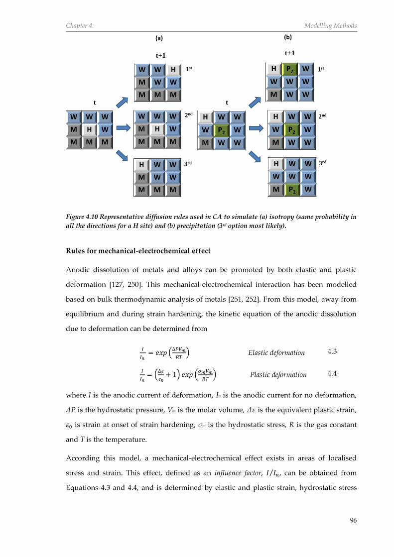
Chapter 4. Modelling Methods
96
Figure 4.10 Representative diffusion rules used in CA to simulate (a) isotropy (same probability in
all the directions for a H site) and (b) precipitation (3rd option most likely).
Rules for mechanical-electrochemical effect
Anodic dissolution of metals and alloys can be promoted by both elastic and plastic
deformation [127, 250]. This mechanical-electrochemical interaction has been modelled
based on bulk thermodynamic analysis of metals [251, 252]. From this model, away from
equilibrium and during strain hardening, the kinetic equation of the anodic dissolution
due to deformation can be determined from
𝐼
𝐼𝑛 = 𝑒𝑥𝑝 (
∆𝑃𝑉𝑚
𝑅𝑇) Elastic deformation 4.3
𝐼
𝐼𝑛= (
∆𝜀
𝜀0+ 1) 𝑒𝑥𝑝 (
𝜎𝑚𝑉𝑚
𝑅𝑇) Plastic deformation 4.4
where I is the anodic current of deformation, In is the anodic current for no deformation,
ΔP is the hydrostatic pressure, Vm is the molar volume, Δε is the equivalent plastic strain,
휀0 is strain at onset of strain hardening, σm is the hydrostatic stress, R is the gas constant
and T is the temperature.
According this model, a mechanical-electrochemical effect exists in areas of localised
stress and strain. This effect, defined as an influence factor, 𝐼 𝐼𝑛⁄ , can be obtained from
Equations 4.3 and 4.4, and is determined by elastic and plastic strain, hydrostatic stress
W W W
M H W
M M M
W W H
M W W
M M M
W W W
M H W
M M M
H W W
M W W
M M M
t+1
t
1st
2nd
3rd
H W W
W P2 W
M W W
t
t+1
H P2 W
W W W
M W W
H W W
W P2 W
M W W
H W W
W W W
M P2 W
1st
2nd
3rd
(a) (b)

Chapter 4. Modelling Methods
97
and pressure stress all of which are obtained from FEA. The magnitude of this factor is
used to specify a probability for changing a metal site from a base state to a reactive state.
4.4.2 Finite element analysis of pit geometry
The dynamic localised stress and strain induced by the growing pit were computed after
five CA time steps using plain strain FEA. Matlab® [249] scripting language was also
used to develop the algorithm that (i) exports the output matrix from the CA, (ii)
automates the relevant parts of the procedure described in Section 4.3.4, (iii) creates an
ABAQUS input file, (iv) creates and submits the job to the ABAQUS standard solver, (v)
uses a python script to output stress and strain tensors from each element, (vi) evaluates
the influence factor based on information on stress and strains, and (vii) modifies the CA
matrix (geometry) accordingly based on the influence factor. Because boundary
conditions and stresses must be applied to continuous surfaces during FE analysis, it was
necessary to ensure that the cells in the boundaries of the metal space do not corrode. This
was achieved by excluding the boundary cells in the metal space from the corrosion
process. Tensile load was applied to evaluate the effect of stress on localised corrosion and
the dynamic strains resulting from a growing pit. The ABAQUS input file is given in
Appendices E1. Because the CAFE model requires the outputs of the FEA as inputs for the
CA, the FEA results were processed further using a subroutine, written in Python
scripting language (Appendix E2), that accesses the ABAQUS output database (.odb file)
and exports the components of the stress, total strain and principal plastic strain tensors in
each element. The parameters in Equation 4.3 and Equation 4.4 were then evaluated from
the stress and strain tensors. The model constants are: Vm = 7.0923×10⁻⁶ m3.mol-1 (for iron),
T = 298 K and R = 8.314 m2 kg s-2 K-1 mol-1. The strain at on-set of strain hardening is taken
as 2%.

Chapter 5
Experimental Results
and Discussion

Chapter 5. Experimental Results and Discussion
99
5.1 Introduction
This chapter presents the results obtained from the present investigations carried out
on API 5L X65 linepipe steel in the as-received condition. The results are presented based
on the main objectives of the experimental part of this research, which include:
1. To characterise the microstructural properties of the material.
2. To establish the baseline mechanical (tensile and fatigue) properties of the material
in air.
3. To establish the basic electrochemical properties of the material.
4. To evaluate pit growth behaviour with and without stress.
5. To evaluate the initiation and propagation behaviour of cracks emanating from
pits in air and aggressive environment.
6. To evaluate the effect of proximity between pits on the initiation and propagation
behaviour of cracks emanating from them.
7. To evaluate the effect of aggressive environment on fatigue endurance behaviour
when corrosion pits are present.
5.2 Material Characterisation
5.2.1 Microstructure
The material was composed mainly of polygonal ferrite grains and equiaxed ferrite grains
(Figure 5.1). Because carbon is present in the material, some amounts of pearlite
microstructure will be expected. However, as can be seen in these micrographs, none was
observed optically, probably due to the very low carbon content (0.05% maximum). From
the analyses of the grain sizes using the linear intercept method [253] and electron
backscattered diffraction (EBSD)3, an average grain size of 15 µm was adopted for the
material. Figure 5.1 also shows that the shapes and sizes of grains in both longitudinal
and long transverse directions are similar but different in the short transverse direction.
The orientation of the longitudinal axis of all the samples used for tensile, cyclic and
fatigue tests was along the longitudinal direction of the pipe.
3 EBSD analysis was carried out by Dr. Yuan Feng Yang of School of Materials, University of Manchester.

Chapter 5. Experimental Results and Discussion
100
Figure 5.1 (a) Schematic of the three directions in a pipe section; and optical micrographs showing
microstructure of the parent plate region of X65 linepipe steel in (b) longitudinal (c) long
transverse and (d) short transverse directions.
5.2.2 Micro-hardness
Figure 5.2 shows the micro-hardness profile in two randomly chosen regions in material.
The average micro-hardness is 206 ± 8 Hv1.0.
Distance from reference line (mm)
0 2 4 6 8 10
Vic
kers
Hard
ness (
HV
1.0
)
190
200
210
220
230
Region 1
Region 2
Figure 5.2 Micro-hardness measurements on X65 steel.
(a) (b)
20 µm
(c)
20 µm
20 µm
(d)

Chapter 5. Experimental Results and Discussion
101
5.2.3 Open circuit potential
In the pit generation procedure and pit growth studies, an anodic potential was applied
with reference to the open circuit potential (OCP) while for corrosion fatigue experiments,
tests were carried out at the free corrosion potential. It was therefore important to
establish this basic electrochemical characteristic of the material in the test environments.
The OCP was monitored in naturally aerated 0.6 M NaCl and brine. The former was
chosen as the test solution for generating pits on fatigue samples and for pit growth
studies in order to overcome the salt crystallisation issue, which was associated with
using the brine (≈ 1.48 M NaCl). Figure 5.3 shows that the free corrosion potential shifted
to more negative values but eventually stabilized with immersion time. The shift towards
the negative direction can be attributed to the progressive degradation of the poor oxide
film on the surface of the steel coupled with the static nature of the test, which limits the
transport of oxygen (cathodic reactant in aerated solution) to the electrolyte-material
interface [15, 254]. This in turn decreases the resistance to the transfer of electrons across
and increases electrochemical activity at the electrolyte-material interface. The stabilized
OCP value was more positive in 0.6 M NaCl (-600 ± 6 mV) than in the Forties brine (-667 ±
5 mV) indicating that the brine is more aggressive (reflecting the higher chloride
concentration) and corrosion rates are more likely to be higher than in 0.6 M NaCl under
the same conditions.
Time x 10-3 (s)
0 20 40 60
Pote
ntial (m
V/A
gA
gC
l)
-700
-650
-600
-550
-500
-450
-400
0.6 M NaCl
Brine
Figure 5.3 OCP measurements in naturally-aerated environments at room temperature.

Chapter 5. Experimental Results and Discussion
102
5.3 Stress-strain properties
5.3.1 Tensile stress-strain behaviour
The deformation response of the material under monotonic loading was evaluated in air
at room temperature. A total of four tests were carried out to establish this. Figure 5.4
shows the representative true and engineering tensile stress-strain curve (MSSC) for the
steel. The material shows discontinuous yielding phenomenon that is peculiar to bcc
(body-centred cubic) materials containing carbon and nitrogen as interstitial atoms [255].
The evaluated tensile properties together with the parameters that define the hardening
behaviour (assumed to be isotropic) are listed in Table 5.1. Some of these properties were
used to define the elastic-plastic material model used for finite element analysis of stress
and strain in Chapter 6.
Strain (%)
0 5 10 15 20 25 30
Str
ess (
MP
a)
300
400
500
600
700
Engineering Stress-Strain Curve
True strain Stress-Strain Curve
Figure 5.4 Monotonic stress-strain curve for X65 steel at room temperature.
5.3.2 Cyclic stress-strain behaviour
This investigation was carried out to understand the cyclic deformation behaviour i.e. the
evolution and mechanisms of damage when this material is subjected to inelastic cyclic
loading. The cyclic mechanical properties were evaluated from the cyclic stress-strain
curve (CSSC), which was obtained by joining the locus of the tips of the stabilized
hysteresis loops that were obtained at different applied strain ranges. The plastic portion
of the CSSC can be written in the form [256]
Necking

Chapter 5. Experimental Results and Discussion
103
∆𝜎
2= 𝐾′ (
∆휀𝑝
2)
𝑛′
5.1
where 𝐾′ is the cyclic hardening coefficient, ∆𝜎 is stress range, ∆휀𝑝 is plastic strain range
and 𝑛′ is the cyclic hardening exponent.
Table 5.1 Tensile properties of X65 linepipe steel at room temperature.
Property Value
Elastic modulus, E (GPa) 211 ± 1
Upper yield strength, YSU (MPa) 520 ± 2
Lower yield strength, YSL (MPa) 516 ± 4
Ultimate tensile strength, UTS (MPa) 614 ± 3
Percentage elongation, %El 15.72 ± 1
Percentage reduction area, %RA 84.11 ± 5
Strength coefficient, K (MPa) 910 ± 8
Strain hardening exponent, n 0.127 ± 0.02
True fracture strength, 𝜎𝑓 (MPa) 1034 ± 25
True fracture ductility, 휀𝑓 (%) 91.63 ± 3
Figure 5.5 shows the CSSC with the tensile curve (MSSC) superposed on it. An
intersection can be observed between the MSSC and CSSC in the hardening region. This
indicates that in the range of strain that was studied, the material exhibits both hardening
and softening (mixed-type) behaviour. The cyclic mechanical properties obtained from
the CSSC are given in Table 5.2. The cyclic yield strength was evaluated at 0.2% offset.
Similar responses have been observed for carbon steel [257-261]. In the region of the CSSC
that lies below the MSSC, cyclic softening occurs while above it, cyclic hardening takes
place. This shows that the cyclic behaviour of the material depends on the applied or
prevailing strain level. Furthermore, the cyclic yield strength is smaller than the tensile
yield strength.

Chapter 5. Experimental Results and Discussion
104
Figure 5.5 Cyclic stress-strain curve for X65 linepipe steel at room temperature.
Table 5.2 Cyclic properties of X65 linepipe steel at room temperature.
Property Value
Cyclic yield strength, YS′(MPa) 420 ± 13
Fatigue strength coefficient, 𝜎𝑓′ (MPa) 802 ± 12
Fatigue strength exponent, b −0.068 ± 0.004
Fatigue ductility coefficient, 휀𝑓′ 0.372 ± 0.031
Fatigue ductility exponent, c −0.584 ± 0.022
Cyclic strength coefficient, 𝐾′(MPa) 923 ± 8
Cyclic strain hardening exponent, 𝑛′ 0.118 ± 0.012
Transition life, 𝑁𝑇(cycles) 7000
5.3.2.1 Evolution of stress and strain
Evolution of the cyclic stress as a function of cycles and as a function of life ratio (ratio of
cycle number to the fatigue life – 𝑁 𝑁𝑓⁄ ) at different strain amplitudes, is shown in Figure
5.6a and Figure 5.6b respectively All the curves exhibit three different regions, namely: a
transient region where the stress amplitude changes rapidly with the number of cycles
(up to 10% of fatigue life); a cyclic saturation region where there is little or no change in
stress amplitude (up to 80% of fatigue life); and a region with a rapid decrease in stress
which can be correlated to the crack propagation process because of the reduction in area
available to support the stress. During cyclic loading of the material, an increase or

Chapter 5. Experimental Results and Discussion
105
decrease in the stress amplitude with increase in number of cycle, indicates cyclic
hardening and softening respectively [262]. Figure 5.6a and Figure 5.6b appears to show
only a general decrease in stress amplitude with number of cycles at all strain amplitudes.
However, observations made in the first few cycles (Figure 5.6c) show that at relatively
high strain amplitudes (> 0.8%), the stress amplitude increases before progressively
decreasing. At total strain amplitudes between 0.3% and 0.65%, only cyclic softening can
be observed since the stress amplitude decreased continuously starting from the first
cycle. In contrast, at 0.8%, 1% and 1.2%, cyclic softening was preceded by an initial period
of cyclic hardening.
Number of Cycles
500 1000 1500
Str
ess a
mplit
ude (
MP
a)
350
400
450
500
550
600
0.50%
0.65%
0.80%
1.00%
1.20%
Life ratio
0.0 0.2 0.4 0.6 0.8 1.0
Str
ess A
mplit
ude (
MP
a)
300
350
400
450
500
550
600
0.30%
0.50%
0.65%
0.80%
1.00%
1.20%
(a)
(b)

Chapter 5. Experimental Results and Discussion
106
Number of Cycles
2 4 6 8 10 12 14 16 18 20
Str
ess A
mplit
ude (
MP
a)
500
520
540
560
5800.30%
0.50%
0.65%
0.80%
1.00%
1.20%
Figure 5.6 Evolution of the stress amplitude (a) with number of cycles; (b) with life ratio; (c) in the
first 20 cycles for different values of strain amplitudes.
This result is consistent with Figure 5.5 and shows that the material exhibits a cyclic
deformation behaviour (hardening and softening) that is dependent on strain amplitude.
Figure 5.7 shows that, in the strain ranges tested, the plastic strain amplitude increases
with increase in number of cycles and with total strain. In terms of plastic strain
amplitude, a decrease with number of cycles indicates cyclic hardening while an increase
indicates softening behaviour [255, 262]. From studies on the cyclic deformation
behaviour of steels, it has been shown that cyclic plastic strain is accompanied by
evolution and modification of the internal structure of the material [260, 261, 263]. The
internal substructure is modified through creation and rearrangement of dislocation
structures, which may involve changes in dislocation density and formation of
microstructures with different substructures depending on level of loading. These
ultimately lead to the observed macroscopic stress-strain response behaviour i.e. cyclic
hardening and cyclic softening. However, the accompanying changes are limited to the
initial period of cycling. Beyond this initial period i.e. in the stabilised region, and for the
majority of the fatigue life, persistent slip bands (PSBs), in which the cyclic plastic strain is
concentrated and redistributed, are formed. As a result of this redistribution, the cyclic
stress-strain response is stabilized and the internal structure of the PSBs is modified [264].
The PSBs lead to the formation of extrusions and intrusions from which cracks are
initiated [255, 264].
(c)

Chapter 5. Experimental Results and Discussion
107
Number of Cycles
0 500 1000 1500
Pla
stic S
train
Am
pltiu
de (
%)
0.2
0.4
0.6
0.8
1.0 0.50%
0.65%
0.80%
1.00%
1.20%
Figure 5.7 Evolution of plastic strain amplitude with number of cycles.
Figure 5.8 presents an example of the surface of a specimen tested at 1% strain amplitude;
showing evidence of multiple crack initiation sites, which can be correlated with the
relatively large level of plasticity (εp ≈ 0.75%) occurring at this strain level (see Figure 5.7).
It can also be observed that one of the cracks appears to be dominant compared to the
others. The location and orientation of the cracks (parallel to loading direction) suggest
that crack coalescence is a likely crack propagation mechanism.
Figure 5.8 Typical surface of a specimen after testing showing dominant crack and several other
smaller cracks. (Total strain amplitude = 1%; Plastic strain amplitude = 0.75%).

Chapter 5. Experimental Results and Discussion
108
5.3.2.2 Stress-life and strain-life relationships
The results for the low cycle fatigue (LCF) life, notably stress amplitude and the plastic
strain amplitude at half-life, are given in Table 5.3. The table illustrates that an increase in
total strain amplitude resulted in increases in stress amplitude and plastic strain
amplitude and a corresponding decrease in fatigue life. The higher plastic strain
magnitudes observed as the total strain increases suggest that an increase in plasticity
resulted in shorter crack initiation lifetimes; hence the observed shorter LCF lives. The
parameters for the Basquin [42] and Coffin-Manson [43, 44] relationships, which are both
combined into Equations 5.2, were also obtained for this material by separating the total
strain into its elastic and plastic components, as shown in Figure 5.9.
∆휀
2=
𝜎𝑓′
𝐸(2𝑁𝑓)
𝑏+ 휀𝑓
′(2𝑁𝑓)𝑐
5.2
where 𝜎𝑓′ is the fatigue strength coefficient, 휀𝑓
′ fatigue ductility coefficient, Nf is number of
cycles to failure, b is fatigue strength exponent and c is fatigue ductility exponent. These
parameters are also given in Table 5.2. It should be noted that the elastic strain values
have been multiplied by the elastic modulus (E) to obtain values of stress.
Figure 5.9 Fatigue strength life and fatigue ductility life curves for X65 linepipe steel.

Chapter 5. Experimental Results and Discussion
109
Table 5.3 Fatigue results for X65 linepipe steel under symmetric strain cycling.
Strain amplitude (%) 0.30 0.50 0.65 0.80 1.00 1.20
Life (cycles) 13421 1466 1061 625 467 294
Stress amplitude (MPa) 416.4 453.2 475.8 491.1 531.3 536.3
Elastic strain amplitude (%) 0.197 0.215 0.226 0.233 0.252 0.254
Plastic strain amplitude (%) 0.103 0.287 0.428 0.568 0.745 0.938
5.4 Pit growth behaviour
5.4.1 Pit growth under no-flow conditions
Pit propagation kinetics (rate of anodic dissolution) was simulated by potentiostatic
polarization of samples in 0.6 M NaCl for different durations of time in an unstressed
condition. Triplicate tests were carried out. The maximum pit depth and pit width in a
test is the average of measurements obtained from four different cross-sectional profiles of
a pit. The results obtained after characterisation of the pits are summarised in Table 5.4.
Theoretical values of pit depth were evaluated from the measured experimental volume
using Faraday’s relationship (Equation 3.4). Figure 5.10 presents plots of experimental
and theoretical mean values of maximum pit depth versus time. Although the theoretical
values show an overestimation of the experimental pit depths, the correlation between
both is fairly good. Figure 5.10 shows that the rate of pit growth decreased with time but
there is a net increase in depth. Because the tests are with a non-flowing solution, the
decrease in pit growth rate is attributed to a diffusion-control mechanism whereby
corrosion products are not able to diffuse away from within the pit, thus limiting the mass
transport of electrochemical species across the metal-electrolyte interface [5, 140, 265]. In
addition, this condition also means that the cathodic species (dissolved oxygen) is also not
easily transported to the reaction site. The coupling of these processes effectively reduces
the rate of anodic dissolution and consequently the pit growth rate. The aspect ratio
(depth : diameter) is generally used to specify the geometry of a corrosion pit and is also
indicative of the severity of a corrosion pit. This has implications for strain localisation
and crack nucleation behaviour. The evolution of the aspect ratio of the pits, with time,
appears to follow the same trend as pit depth because the experimental conditions confine
the diameter of the pit to that of the width of the microcapillary.

Chapter 5. Experimental Results and Discussion
110
Time (hours)
0 2 4 6 8 10
Maxim
um
pit d
epth
(
m)
50
100
150
200
250
300
350
Experimental
Theoretical
Time (hours)
0 2 4 6 8 10
Maxim
um
pit d
epth
(
m)
50
100
150
200
250
300
350
Pit a
spect ra
tio
0.2
0.4
0.6
0.8
1.0
Pit depth
Aspect ratio
Figure 5.10 Maximum pit depth (a) and pit aspect ratio (b) versus time under static conditions.
Table 5.4 Mean value of pit characteristics obtained at different polarization times.
Time (s) Pit depth (µm) Aspect ratio Pit volume (µm3)
1800 71.5 0.281 11074275
3600 112.5 0.459 17753905
5400 133 0.501 21272460
7200 153.5 0.589 25204056
10800 169.5 0.616 33748293
14400 202.5 0.698 46848960
18000 232.5 0.770 51987840
21600 240 0.777 57473818
25200 264 0.800 70647164
28800 273 0.819 78252603
(a)
(b)

Chapter 5. Experimental Results and Discussion
111
5.4.2 Pit growth behaviour under cyclic stress
The influence of cyclic stress on pit growth behaviour was investigated by carrying out
tests with and without applied stress. Figure 5.11 shows the influence of applied cyclic
stress on pit depth. For the same time interval, pit depths are larger under applied stress
compared to when no stress was applied. This observation is consistent with results from
previous studies [117, 124, 127, 250, 251] where relatively larger pit sizes were found with
increasing applied stress. The effect of applied stress on pit growth is generally attributed
to stress-assisted dissolution through increased local electrochemical activity [266, 267].
The strain localisation effect of the pit increases local activity of dislocations to which
higher energy state atoms are associated. The less activation energy required to remove
these atoms results in preferential electrochemical attack, thereby promoting dissolution
of the steel matrix around the pit [268]. It was also observed from Figure 5.11 that the
difference between the two sets of data tends to increase with time. This can also be
associated with the mechanical-electrochemical effect of strain localisation on localised
corrosion. Pit size becomes larger with time and the instantaneous magnitude of strain
due to strain localisation also increases. This is expected to further increase dissolution
rate and pit depth over time.
Time (hours)
0 10 20 30 40
Maxim
um
pit d
epth
(
m)
200
400
600
800
1000
No stress
= 180 MPa
Figure 5.11 Dependence of pit growth rate on cyclic stress.

Chapter 5. Experimental Results and Discussion
112
5.5 Fatigue and corrosion fatigue behaviour
In the present study, fatigue behaviour of plain and pre-pitted specimens was
investigated in air and an aggressive environment. Specifically, tests were carried out to
understand the influence of stress level, pit size (pit size subsequently refers to pit aspect
ratio and pit depth) and operating environment on the behaviour of cracks emanating
from corrosion pits. Plain (un-pitted) specimens were tested in air at stress ranges
between 432 and 495 MPa to establish the baseline fatigue behaviour in air for evaluating
the effects of pitting in air (mechanical) and corrosive environment (mechanical and
corrosion) on fatigue behaviour. For single-pitted specimens tested in air and corrosion
fatigue, three pit depths of 140 µm (𝐴𝑅𝑝 = 0.52), 200 µm (𝐴𝑅𝑝 = 0.68), and 270 µm (𝐴𝑅𝑝 =
0.82) were chosen while stress range was varied between 350 and 450 MPa. In testing of
double-pitted specimens, two stress ranges (427.5 and 405 MPa) and two pit depths: 200
µm (𝐴𝑅𝑝 = 0.68), and 270 µm (𝐴𝑅𝑝 = 0.82) were chosen while the centre-to-centre distance
between the double pits (both having similar aspect ratios) varied between 0.68 and 1.94
mm. Figure 5.12 shows examples of single and double pits with different aspect ratios and
separation distances. In some cases, when crack initiation was observed and/or during
crack propagation, test specimens were unmounted so that optical and SEM images of the
cracks could be obtained.
Figure 5.12 Optical images showing single pit (dp = 202 µm, ARp = 0.67) in (a) and double pits in
(b&c) with similar aspect ratios but different distances separating them: (b) dp.avg = 197 µm, ARp.avg
= 0.69, see = 105 µm, scc = 693 µm (c) dp.avg = 199 µm, ARp.avg = 0.68, see = 479 µm, scc = 1066 µm.
500 µm 500 µm 500 µm
(a)
(c) (b)

Chapter 5. Experimental Results and Discussion
113
5.5.1 Crack initiation behaviour
In order to study the initiation behaviour of cracks emanating from pits, crack initiation
sites and crack initiation lives were analysed and evaluated as a function of pit size, stress
level and test environment in single and double-pitted specimens. The crack initiation site
is the region around the pit where a crack was found while the crack initiation life is the
number of cycles at which a crack was first observed. Because cracking was monitored at
intervals, it was impossible to determine the exact cycle number at which a crack initiated
during the fatigue life. Hence, for all experiments, the crack initiation life and the
corresponding crack length at initiation were defined as:
𝑁𝑖 = 𝑁2− 𝑁1
2 5.3
𝑎𝑖 = 𝑎2 5.4
where Ni is the crack initiation life, N2 is number of cycles where a crack was first
observed, N1 is the number of cycles at the last interval (before crack initiation), ai is crack
length at initiation and a2 is the crack length corresponding to N2.
5.5.1.1 Plain specimens
Where there was cracking on plain (un-pitted) specimens, cracks initiated at either and/or
the corners or the edges of the fatigue specimen (within the dog bone gauge section).
Figure 5.13 shows an example of a crack that initiated from the edge of a specimen. In
samples that did not fail, no evidence of non-propagating cracks was found. Given that
the edges of the specimens were longitudinally polished and rounded, to eliminate any
premature crack nucleation as a result of artefact surface defects produced during
machining, it is thought that some of the cracks might also have initiated from very small
mechanical and microstructural imperfections. Further fractographic analyses will be
required to confirm this (discussed later).

Chapter 5. Experimental Results and Discussion
114
Figure 5.13 Typical crack initiation from edge of a plain specimen in air (Δσ = 468 MPa, crack
length = 668 µm, N/Nf = 0.84; Nf = 8.27 x 10⁵).
5.5.1.2 Pre-pitted specimens
In all the specimens tested in air, fatigue cracks generally initiated predominantly from
the pit mouth irrespective of stress level and pit size (single pits) and separation distance
(in the case of double pits). The cracks observed on the majority of the double-pitted
specimens emanated from the pit mouth in the region separating the two adjacent pits.
Examples of crack initiation from the pit mouth in single pits in air are shown in Figures
5.14 and 5.15 while Figures 5.16 shows that of double-pits. Because of the size of the
cracks relative to the pits, only the regions around the pit where cracks initiated are
shown. The crack tips are indicated with arrows. Since the tests were conducted in air,
these results suggest that the conditions for crack nucleation are more favourable at the
pit mouth than at the pit bottom. Therefore, localisation of the crack initiation site to the
pit mouth can only be attributed to the mechanical effects of pit shape and size. From
previous studies [9, 105, 121, 202, 269], mechanics-based explanations have been given for
this phenomenon. On the one hand, local yielding under loading conditions may result in
redistribution of stresses around pits thereby leading to localisation of plastic strains at
the pit mouth [121, 202]. On the other hand, if pits are considered to be equivalent to
semi-elliptical cracks, the associated stress intensity factor, which varies along the
periphery of the crack, is maximum at the pit mouth and minimum at the pit bottom [9,
269]. Both of these conditions, coupled with the minimum constraint existing at the
surface of the specimen, where the stress field changes from plain strain in the interior to
plane stress at the surface, facilitates crack nucleation near the pit mouth.
Crack tip

Chapter 5. Experimental Results and Discussion
115
Figure 5.14 SEM image showing initiation of short cracks at the mouth of a pit in air.
(Δσ = 427.5 MPa; dp = 266 µm; ARp = 0.82; Ni = 0.81Nf; Nf = 1.03 x 10⁵).
Figure 5.15 SEM image showing initiation of short cracks at the mouth of a pit in air.
(Δσ = 450 MPa; dp = 142 µm; ARp = 0.52; Ni = 0.52Nf; Nf = 7.51 x 10⁵).
Figure 5.16 SEM images showing initiation of short cracks from the mouth of double pits in air. (a)
Δσ = 427.5 MPa, dp = 265 µm, AR = 0.79, see = 398 µm, scc = 1063 µm, Ni = 0.76Nf, Nf = 7.64 x 10⁵
cycles (b) Δσ = 427.5, dp = 268 µm, ARp = 0.83, see = 207 µm, scc = 857 µm, Ni = 0.37Nf, Nf = 5.06 x 10⁵
cycles.
In all the double-pitted specimens tested in air, the pit mouth was also found to be the
preferred site for crack initiation irrespective of stress level, pit size and separation
10 µm
5 µm 5 µm
5 µm 5 µm
10 µm
(a) (b)

Chapter 5. Experimental Results and Discussion
116
distance. Moreover, the cracks emanated in the region separating the two pits i.e. the
region defined by the edge-to-edge distance, 𝑠𝑒𝑒 (see Figure 3.8 for definition of 𝑠𝑒𝑒). This
suggests that the condition for crack initiation is more favourable at the pit mouth and in
the region separating the two pits. It is thought that the proximity of any two pits will
result in an interaction between their stress and/or strain fields. Consequently, strain
levels may increase in this region and thereby result in a higher tendency for crack
nucleation. Further FE analyses carried out to correlate these observations with
interaction between strain distribution around the pits are reported in Chapter 6.
Due to the strain localisation around the pits, it is expected that cracks should initiate at
both sides of a pit after a similar number of cycles. In general, this was not found to be
true. In some of the single-pitted specimens, the crack initiation lives for both cracks
emanating from adjacent sides of the pit differed in 60% of the tests, but not significantly.
Because this difference could not be correlated with pit size and stress range, it is thought
that this behaviour may be due to stochastic nature of crack initiation. Another possibility
is the non-uniform localisation of strain that may have resulted from the real shape of the
pit, which likely concentrated strain to one side of the pit more than the other. Similar
observations were made on double-pitted specimens where the majority of the cracks
initiated at only one of the two pits, except in few cases where cracks initiated at both pits
together. Furthermore, in this case, no correlation was found with pit size, stress level and
separation distance. In addition to the explanation given for the single pit samples, it is
thought that the differences in strain distribution due to variation in the true pit sizes may
be a contributing factor for double pits. It should be noted that only mean values of the
sizes of the double pits are reported in the results whereas, in reality, the depths of the
pits may vary by up to ± 5%. Hence, it is expected that the higher strain localization
associated with relatively deeper pits might favour cracking. However, further analyses of
the experimental data showed that majority of the crack-initiating pits were not always
the pits with a relatively greater depth or aspect ratio.
Observations from previous studies have shown that cracks can initiate from the mouth
[9, 121] as well as the pit bottom [189, 195]. The present results appear to show that cracks
only initiate from the pit mouth. However, no conclusion can be made at this point
because the replica method used in this study only permitted detection of surface cracks.
Therefore it was important to ascertain whether cracks also initiated from other regions

Chapter 5. Experimental Results and Discussion
117
other than the pit mouth. For corrosion fatigue tests, this was not a problem because the
crack observation technique used was capable of detecting cracks everywhere around the
pit. For the tests carried out in air, crack initiation from the pit bottom was assessed by
fractography. The results from fracture surface analysis are reported in a Section 5.6.
In the tests carried out on single-pitted specimens in the Forties brine solution, cracks
were found to initiate from both the mouth and bottom of pits. In previous work on
HSLA steels with properties similar to the steel used in this work, cracks were found to
initiate from the pit bottom [122, 270] while in other steel-environment systems, cracks
initiated from the pit mouth [9, 105, 121, 269] as well as the pit bottom [169, 189, 269].
Figure 5.17 shows crack initiation from the different locations, notably; only the pit mouth
(Figure 5.17a), the pit bottom (Figure 5.17b) or both mouth and pit bottom (Figure 5.17c).
Table 5.5 summarises observations of crack nucleation sites with stress and pit size.
Although no apparent correlation was found with pit size and stress level, the results
generally suggest that crack initiation at the pit bottom tends to occur at relatively lower
stresses and smaller pit size respectively. The only case where cracks initiated at the pit
mouth occurred in the pit with depth of 270 µm (ARp = 0.82) tested at the highest applied
stress range (450 MPa). Comparison with the corresponding test carried out in air,
suggests that crack initiation at the pit mouth in the brine solution might be attributed to
the dominance of the mechanical effect of strain localisation at high stresses at the pit
mouth.
Table 5.5 Crack initiation characteristics from pits tested in brine solution.
Stress range
(MPa) ARp = 0.52 ARp = 0.68 ARp = 0.82
360 No data No data Pit bottom
405 Pit bottom Pit bottom Pit mouth and pit bottom
427.5 Pit bottom Pit mouth and pit bottom Pit mouth and pit bottom
450 Pit mouth and pit bottom Pit mouth and pit bottom Pit mouth
At the crack initiation stage, multiple cracks were often observed at the pit bottom and
sometimes at the pit mouth (Figure 5.17b and 5.17c). As cycling continued, more cracks
initiated at the pit bottom some of which coalesced with each other and also with the
cracks that initiated at the pit mouth thus forming bigger cracks. It was interesting to see

Chapter 5. Experimental Results and Discussion
118
that all the multiple cracks that initiated at the pit bottom are always aligned
perpendicular to the loading direction (Figures 5.17b, 5.17c and 5.18a).
Figure 5.17 Typical corrosion fatigue crack initiation behaviour from (a) pit mouth [Δσ = 450
MPa; dp = 271 µm; Ni = 0.66Nf; Nf = 1.9036 x 10⁵], (b) pit bottom [Δσ = 405 MPa; dp = 141 µm; Ni =
0.779Nf; Nf = 4.17 x 10⁵], and (c) pit mouth and pit bottom [Δσ = 427.5 MPa; dp = 202 µm; Ni =
0.813Nf; Nf = 3.75 x 10⁵]. Loading direction is from top to bottom.
To gain more insight, the test in Figure 5.18a was aborted and the specimen was cleaned,
dried and examined on the SEM. Figure 5.18b shows an SEM image of the pit (with
multiple crack initiation sites at the pit mouth and bottom). The main observation is that
not all the cracks, which appear at the bottom of the pit, have extended into the specimen.
For the cracks that have extended into the specimens, it appears that only those that are
aligned with the cracks at the pit mouth, and perpendicular to the loading direction,
became damaging i.e. coalesced with other cracks to form a larger crack. These results,
which show crack initiation at the pit bottom at stress levels where no cracks were
(a) (b)
(c)

Chapter 5. Experimental Results and Discussion
119
observed at the pit bottom in air, suggest that the conditions for crack initiation were
modified in the aggressive environment. One possible mechanism is that of strain-assisted
dissolution of slip steps (combined with film rupture) resulting from the strain
localization effect of the pit. Under cyclic loading, slip bands may be induced around the
pit due to localised deformation [270]. The higher energy state of metal atoms associated
with dislocations reduces the activation energy is required to remove the atoms from the
material [268, 271]. Consequently, the aggressive environment will lead to preferential
dissolution of the slip steps and promote crack initiation. In addition, electrochemical
changes within the pit, such as changes in local solution composition, pH and
electrochemical potential may also play an important role in the crack initiation
behaviour. Further discussions on these factors in the context of the observations made in
this study will be presented in Chapter 8.
Figure 5.18 Typical corrosion fatigue crack initiation behaviour from pits (a) optical and (b) SEM
images. (Δσ = 427.5 MPa; dp = 266 µm; ARp = 0.82; Ni = 0.754Nf; Nf = 3.13 x 10⁵). Loading direction is
from left to right.
5.5.1.3 Crack initiation lifetime
Single pits – fatigue tested in air and brine solution
Figure 5.19a shows the influence of pit size and stress level on crack initiation lifetimes in
air and brine solution. For a given stress level and pit size, the crack initiation life (Ni)
decreased with increase in pit size and increase in stress level respectively. These trends
were observed in both air and brine environment, thus showing that the overall influence
(a) (b)

Chapter 5. Experimental Results and Discussion
120
of pit size and stress level on crack initiation behaviour from pits in this material appears
to be test environment independent (at these stress levels). This observation is consistent
with reports from previous studies on steel-brine systems [16, 122] and can be attributed
to the mechanical effects of pit size and applied stress on strain localisation at pit sites. An
increase in the pit size and stress level increases the magnitude of the local strain around a
pit and consequently result in greater susceptibly to early crack nucleation [1, 270]. Figure
5.19a also shows a significant reduction in the crack initiation life in the aggressive
environment, compared to air, at all stress levels. The interaction between localised strain
and the environment is expected to further increase susceptibility to cracking through
strain-enhanced dissolution of slip steps [271-273]. Therefore, it easier for cracks to initiate
in a shorter time in the presence of the environment. Comparison between the crack
initiation life plotted as a fraction of fatigue life in air and brine solution is shown in
Figure 5.19b. The notable observation here is that the fractions of lifetime taken for crack
nucleation are generally higher than 60%. This indicates that the fatigue behaviour of the
steel when pits are present depends more on initiation than propagation of cracks.
However, the extent of this dependency is relatively greater in air (70-100%) than in
corrosion fatigue (65-85%). Note that 100% fraction of lifetime represents a sample on
which no crack was found or did not fail after 107 cycles.
Stress range (MPa)
0 20 40 60 80 100
Cra
ck initia
tion life (
cyc
les)
105
106
107
dp = 140 m (ARp = 0.52)
dp = 200 m (ARp = 0.68)
dp = 270 m (ARp = 0.82)
450 427.5405
(a)

Chapter 5. Experimental Results and Discussion
121
Stress range (MPa)
0 20 40 60 80 100
Ni/N
f (%
)
60
70
80
90
100
110
120
dp = 140 m (ARp = 0.52)
dp = 200 m (ARp = 0.68)
dp = 270 m (ARp = 0.82)
450 427.5405
Figure 5.19 Comparison between crack initiation lives in air and brine solution for different stress
levels and pit sizes as function of (a) number of cycles and (b) fraction of total lifetime. [Plain bars
= Air; Hatched pattern bars = Corrosion fatigue].
Double pits – fatigue tested in air
The relationship between crack initiation life and centre-to-centre distance (subsequently
referred to as separation distance) between double pits, for different pit sizes and stress
levels, is shown in Figure 5.20a. As a reference, corresponding values obtained for single
pits are also shown as horizontal lines on the figure. For all the pit sizes and stress levels
studied, a dependency was found between crack initiation lifetime and separation
distance between pits, up to a pit-to-pit separation distance of about 1400 µm. Below this
separation distance, Ni generally decreased with decrease in separation distance. This
indicates that the closer the pits are to each other, the shorter the crack initiation life.
Furthermore, at the same separation distance, stress and pit size influenced crack
initiation life. At a given stress level, Ni was relatively lower for a deeper pit (or larger
aspect ratio) and vice versa. Similarly, at a given pit aspect ratio, Ni decreased when the
stress range increased from 405 to 427.5 MPa. Since these tests were carried out in air,
these results only show the effect of the mechanical interaction between double pits on
crack initiation life. This interaction can be related to the stress and strain fields around
the pits, which depend on pit size and applied stress [1, 201, 204]. The smaller the
(b)

Chapter 5. Experimental Results and Discussion
122
separation distance, the greater the mechanical interaction between pits and the higher
the tendency for the pit to transition to a crack. The dependence of crack initiation life on
pit size and applied stress is attributed to the strain localisation effect of the pits [201, 234].
At a given stress level, increase in pit size will result in greater strain localisation and for a
given pit size, increasing the applied stress level will have similar effect. In all cases, the
overall consequence is a higher tendency to initiate a crack and therefore decrease the
crack initiation life. The present results show that the nucleation of cracks from pits
depends on pit size, applied stress and proximity of pits to each other.
To quantify the effect of pit proximity on overall fatigue life, crack initiation lifetimes
were plotted as a fraction of the total fatigue life (Figure 5.20b). A horizontal has been
drawn on this figure to indicate the mean of the percentage crack initiation lifetimes
obtained for 200 and 270 µm deep single pits cycled at Δσ = 405 and 427.5 MPa. A single
horizontal line was used because the difference between the percentage crack initiation
lifetimes for both pit depths at these two stress ranges was less than 6%. The main
observation is that, depending on separation distance, the interaction between pits
significantly reduced the fraction of the total fatigue required for crack initiation. Whereas
crack initiation life was up to 95% of the fatigue life in the case of single pits, it can be
reduced by as much as a factor of five to about 20% when there is interaction between the
pits. The increase in percentage crack initiation life from about 20% at short separation
distances to about 95% at relatively longer distance indicates that the fatigue behaviour
changed from being dominated by crack propagation, to that of crack initiation, as the pits
become further apart. These results suggest that the fatigue behaviour of the material can
change from being initiation-dominant to propagation-dominant when multiple pits
interact with each other.
It can also be observed in Figure 5.20a that the trends in increase in crack initiation life
appear to be exponential and also tended towards maximum values that are similar to
those obtained for single pits (indicated with horizontal lines). From these results, there
appears to be a threshold, separation distance, beyond which there is little interaction
between pits, in terms of the influence on crack initiation life. This threshold distance was
found to be dependent on the applied stress level and pit aspect ratio. For instance,
increasing the stress level from 405 to 427.5 MPa increased the threshold distance required

Chapter 5. Experimental Results and Discussion
123
to mitigate the combined effect of the pits on crack initiation. The threshold distances
evaluated from Figure 5.20a as the distance when the trend line intersects the horizontal
lines representing the crack initiation lives for the single pits are given in Table 5.6. The
results show that the threshold distance increased with increase in pit size and stress
range.
Center-to-center distance (m)
600 800 1000 1200 1400
Cra
ck initia
tion life, N
i (c
ycle
s)
105
106
107
ARp = 0.68 ( = 405 MPa)
ARp = 0.82 ( = 405 MPa)
ARp = 0.68 ( = 427.5 MPa)
ARp = 0.82 ( = 427.5 MPa)
Center-to-center distance (m)
600 800 1000 1200 1400
Ni/N
f (%
)
0
20
40
60
80
100
ARp = 0.68 ( = 405 MPa)
ARp = 0.82 ( = 405 MPa)
ARp = 0.68 ( = 427.5 MPa)
ARp = 0.82 ( = 427.5 MPa)
Figure 5.20 Crack initiation lives versus separation distance between two pits as a function of pit
size and applied stress plotted in (a) number of cycles and (b) fraction fatigue life. Horizontal lines
represent corresponding values for single pits.
(a)
(b)
ARp = 0.68
(Δσ = 405 MPa)
ARp = 0.82
(Δσ = 405 MPa)
ARp = 0.82
(Δσ = 427.5 MPa)
ARp = 0.68
(Δσ = 427.5 MPa)
Mean percentage
crack initiation
lifetime for single pits

Chapter 5. Experimental Results and Discussion
124
Table 5.6 Estimated threshold values for separation distances between double pits.
Stress range (MPa) dp = 200 µm (ARp = 0.68) dp = 270 µm (ARp = 0.82)
405 860 1040
427.5 980 1210
5.5.2 Crack propagation behaviour
5.5.2.1 Crack development from pits in air
Typical behaviour of the cracks that initiated from single and double pits in air are shown
in Figure 5.21 and Figures 5.22—5.23 respectively. For single pits, cracks initiated from
adjacent sides of the pit mouth and propagated in the direction perpendicular to the
applied stress until failure of the specimen (Figure 5.21). No evidence of crack branching
was found. In some cases, where a crack initiated from only one side of the pit mouth, a
delay in cycles was observed before a second crack initiate from the adjacent side of the
pit mouth. In the tests where this occurred, the delay in crack initiation times is thought to
be random as no correlation was found between the loading conditions and pit sizes.
N/Nf = 0 N/Nf = 0.986
N/Nf = 0.996 N/Nf = 0.998
Figure 5.21 Typical air fatigue crack development from single pits. Images obtained from replicas.
Δσ = 405 MPa, dp = 265 µm, ARp = 0.81, Ni = 5.025 x 10⁵ cycles, Nf = 5.205 x 10⁵ cycles. Arrows
indicate crack tips and loading direction is from left to right.

Chapter 5. Experimental Results and Discussion
125
Crack initiation behaviour for double-pitted specimens exhibited different behaviour.
When only a single crack initiated at the mouth of one of the pits, as was observed in the
majority of the tests, it propagated perpendicularly to the loading direction into the
adjacent pit (Figures 5.22 - 5.23). When two cracks initiated from each of the adjacent pits,
each crack propagates until coalescence occurs (Figures 5.24 - 5.25). It has been suggested
that when two cracks are close enough, the mechanical interaction of the plastic zones at
each of the leading crack tips may cause both cracks to coalesce, causing an abrupt
increase in crack size and acceleration of crack growth [274-277]. It is interesting to note
that deviations in the adjacent crack tips take place just before coalescence occurs. The
deviation is more notable in Figure 5.25 than in Figure 5.24, possibly being due to the
slight offset in the mid-planes of the adjacent pits. Similar observations reported by other
authors [275, 278-280] were attributed to the fact that it is energetically unfavourable for
any two adjacent crack-tips to extend without such deviations. As noted by Forsyth [280],
crack tip offset distance and stress intensity factor level effects determine the conditions
for crack coalescence. It is apparent from Figures 5.24 and 5.25 that the closeness between
the tips of the cracks appears to have facilitated the interaction of the plastic zones at each
of the crack tips, causing both cracks to coalesce. This interaction will also reduce the
tendency of the cracks following crystallographic paths. A schematic of this process is
shown in Figure 5.26. Since, there is a greater offset distance in Figure 5.25, the plastic
zone interaction will be more pronounced and the deviation will be greater than in Figure
5.24.
Another notable observation from Figures 5.24 and 5.25 is that the two cracks appear to
have different growth rates prior to coalescence, with one crack propagating at a rate
faster than the other. From observations made at intervals before coalescence, it appeared
that the smaller crack stopped growing for some time (non-propagating) but re-
propagated just before coalescence occurred. This behaviour may be attributed to the
shielding effect of the larger crack (usually initiated first), which retards the growth rate
of the smaller crack until the latter becomes non-propagating. The is due to the lower
effective stress at the tip of the smaller crack, resulting from the deviation of the lines of
force of the relatively larger crack [281].

Chapter 5. Experimental Results and Discussion
126
N/Nf = 0.41 N/Nf = 0.48
Figure 5.22 Typical fatigue crack development in double-pitted specimens in air. Δσ = 427.5 MPa,
dp(1) = 269 µm, dp(2) = 265 µm, ARp(1) = 0.83, ARp(2) = 0.80, see = 207 µm, scc = 857 µm, Ni = 1.86 x 10⁵
cycles, Nf = 5.06 x 10⁵ cycles. Arrows indicate crack tips and loading direction is from left to right.
N/Nf = 0.71 N/Nf = 0.78
N/Nf = 0.97
Figure 5.23 Typical fatigue crack development in double-pitted specimens in air. Δσ= 405 MPa, dp(1)
= 196 µm, dp(2) = 198 µm, ARp(1) = 0.68, ARp(2) = 0.69, see = 105 µm, scc = 693 µm, Ni = 3.8 x 10⁵ cycles, Nf
= 5.5 x 10⁵ cycles. Arrows indicate crack tips and loading direction is from left to right.
100 µm 100 µm
500 µm
(a) (b)
(c)
(a) (b)
(a) (b)

Chapter 5. Experimental Results and Discussion
127
N/Nf = 0.895
N/Nf = 0.899 N/Nf = 0.917
Figure 5.24 Typical crack coalescence during fatigue crack development in air. Δσ= 427.5 MPa, dp(1)
= 264 µm, dp(2) = 272 µm, ARp(1) = 0.81, ARp(2) = 0.81, see = 525 µm, scc = 1188 µm, Ni = 19.96 x 10⁵ cycles,
Nf = 22.31 x 10⁵ cycles. Loading direction is from left to right.
N/Nf = 0.81 N/Nf = 0.83
Figure 5.25 Typical crack branching during fatigue crack development in air. Δσ = 427.5 MPa, dp(1) =
274 µm, dp(2) = 265 µm ARp(1) = 0.83, ARp(2) = 0.79, see = 398 µm, scc = 1063 µm, Ni = 5.84 x 10⁵ cycles, Nf
= 7.64 x 10⁵ cycles. Loading direction is from left to right.
Point of crack
coalescence
Region of crack tip
deviation and
coalescence
20 µm
200µm
200µm
Crack 2
Crack 1
(a)
(b)
(d) (c)
(a) (b)

Chapter 5. Experimental Results and Discussion
128
Figure 5.26 Schematic showing stages of crack deviation and coalescence involving interaction of
plastic zones on approaching crack tips (after [280]).
It was previously mentioned that there appears to be a threshold separation distance
between pits beyond which the cracking initiation behaviour is similar to that of a single
pit (see Figure 5.20 and Table 5.6). An example where cracks can be seen to initiate and
propagate from only one pit when the separation distance did not influence the crack
initiation lifetime is shown in Figure 5.27. Although the Ni for the single and double pits
may be similar, it was expected that cracks should initiate from both pits since both pits
have similar depth and aspect ratio. However, this was not the case and may be due to
scatter in crack initiation lifetime. For instance, the crack propagation lifetime for this
specimen (3.1 x 10⁵ cycles) may be similar to the scatter in crack initiation lifetime for a
single pit of the same size cycled at the same stress range. In this case, the cracks that
initiated from one pit would likely have propagated to a size that is large enough to
dominate the damage process before cracks could initiate from the other pit.
Irrespective of the different crack propagation behaviour described above, the cracks
propagate, in a direction perpendicular to that of loading, into the adjacent pit. The nature
of propagation of the cracks on the double-pitted specimens made it impractical to
measure crack extension, once a crack propagates to the edge of the adjacent pit or when
two initiated cracks coalesce into a single crack. Therefore, crack propagation data was

Chapter 5. Experimental Results and Discussion
129
only obtained between crack initiation and when a crack propagates to the edge of the
adjacent pit or when two adjacent cracks coalesced.
N/Nf = 0 N/Nf = N/Nf = 0.
Figure 5.27 Typical crack development behaviour in air when there is no interaction between the
strain fields of pits. Δσ = 427.5 MPa, dp(1) = 272 µm, dp(2) = 268 µm ARp(1) = 0.83, ARp(2) = 0.81, see = 703
µm, scc = 1364 µm, Ni = 3.90 x 10⁵ cycles, Nf = 4.18 x 10⁵ cycles. Arrows indicate crack tips and
loading direction is from left to right.
5.5.2.2 Crack development from pits in corrosion fatigue
For corrosion fatigue tests, surface crack extension was monitored in-situ using a digital
microscope. Although the crack initiation behaviour in the aggressive environment
showed that cracks can initiate from the pit bottom, these cracks extended into the
specimen making it difficult to characterise them, in terms of crack extension using optical
observation. An implication of this is that, if a crack initiated first from the pit bottom, the
cycle number at crack initiation and that corresponding to the first crack extension
measurement (at the pit mouth) will be different. This difference was observed to be
significant especially at relatively lower stresses, hence, must be accounted for. Since
crack growth rates are based on surface crack lengths, this difference was only added to
the overall crack initiation life. Figure 5.28 shows typical development of cracks that
initiated from a pit in the brine environment. The white arrows indicate cracks that
initiated from the pit bottom, while the black arrows indicate the cracks that initiated
500µm
(a) (c) (b)

Chapter 5. Experimental Results and Discussion
130
from the pit mouth. In Figure 5.28a, multiple cracks can be observed to have formed at the
mouth and bottom of the pit. Out of the three cracks that initiated from the right side of
the pit mouth, only one became dominant (Figure 5.28b). Similarly, of all the cracks that
seemed to have initiated at the pit bottom, two appeared to have coalesced with other
cracks and thus became dominant. In Figure 5.28c and 5.28d, the dominant cracks at the
pit bottom coalesced with those growing from the mouth and joined at the latter stages of
crack development (Figure 5.28e). In other tests, cracks from the pit mouth and bottom
coalesced during the propagation stage earlier than shown in this example. The fractured
specimen is shown in Figure 5.28f.
N/Nf = 0.864 N/Nf = 0.912
N/Nf = 0.936 N/Nf = 0.983
200 µm
500 µm 500 µm
200 µm
(a) (b)
(c) (d)

Chapter 5. Experimental Results and Discussion
131
N/Nf = 0.99 N/Nf = 1.00
Figure 5.28 Typical corrosion fatigue crack development. White and black arrows indicate cracks
that initiated from pit bottom and the crack tips of those from the pit mouth respectively. Δσ = 405
MPa, dp = 265 µm, ARp = 0.81, Ni = 3.32 x 10⁵ cycles, Nf = 4.19 x 10⁵ cycles. Loading direction is from
top to bottom.
5.5.2.3 Crack growth rates in air and corrosion fatigue
After crack initiation, fatigue crack propagation rates, in both air and brine solution, were
determined by measuring the crack extension ace, which is the crack length extension
beyond the pit mouth. This allows correlation of crack size with short crack behaviour
and dimensions of the microstructure. A schematic of the two is shown in Figure 5.29.
Fatigue crack growth rates, da/dN, were estimated by using the secant method below:
(
𝑑𝑎
𝑑𝑁 )
𝑖+12
= 𝑎𝑖+1 − 𝑎𝑖
𝑁𝑖+1 − 𝑁𝑖
5.5
where ai and ai+1 are two consecutive surface crack lengths at Ni and Ni+1 number of cycles
respectively. Since the fatigue crack growth rate represents the growth of a crack at the
midpoint of two consecutive crack lengths, the corresponding average crack length at this
point is 0.5(ai + ai+1).
500 µm 500 µm
(f) (e)

Chapter 5. Experimental Results and Discussion
132
Figure 5.29 Schematic of surface length and crack extension of cracks that initiated from a pit.
Single pits – fatigue tested in air and corrosion fatigue
Plots of average crack extension from pit mouth versus fraction of fatigue life ((ace)avg –
N/Nf) and crack growth rates (da/dN - (ace)avg) at different stress levels and for different
single pit sizes are shown in Figures 5.30 – 5.36. Cracks that initiate but become non-
propagating are also shown on these plots. The results generally exhibited some scatter,
which was attributed to a number of factors including differences between crack initiation
lives for the two cracks emanating from the two adjacent pit mouth regions, crack
coalescence and the nature of the crack extension monitoring techniques e.g. replicas in
air and digital microscope in brine solution. In addition, the corrosion fatigue data
exhibits more scatter because of the inability to ascertain the exact tip of the fatigue crack
due to surface corrosion, leading to a variation of about 30 µm, giving a scatter of around
3 x 10⁻⁹ m/cycle from the exact value. Nevertheless, all the results show apparent trends in
the data. To assess the influence of the environment, applied stress and pit size on crack
growth behaviour, the results were grouped in terms of pit sizes and stress levels
respectively in both air and brine solution.
Figure 5.30 shows a comparison of plots of crack extension from the pit mouth versus
number of cycles as a fraction of fatigue life for specimens containing 200 µm deep pits
(aspect ratio ≈ 0.68) cycled at different stress levels in air and brine solution. The plots for

Chapter 5. Experimental Results and Discussion
133
a pit depth of 140 µm (aspect ratio ≈ 0.52) cycled at Δσ = 450 MPa are also shown. Figure
5.31 shows similar plots for a 270 µm deep (aspect ratio ≈ 0.82) pit.
N/Nf (%)
70 75 80 85 90 95 100
Avera
ge c
rack e
xte
nsio
n (
m)
0
400
800
1200
= 427.5 MPa
= 450 MPa
= 450 MPa (AR = 0.52)
= 414 MPa
Air
Brine
Figure 5.30 Average crack extension versus fraction of lifetime in air and brine solution at different
stress levels. [dp ≈ 200 µm, ARp = 0.68, R = 0.1, f = air - 15 Hz, brine – 2 Hz]. Crack length data pit
depth of 140 µm (ARp = 0.52) cycled at Δσ = 450 MPa is also shown.
N/Nf (%)
60 70 80 90 100
Avera
ge c
rack e
xte
nsio
n (
m)
0
400
800
1200
= 405 MPa
= 427.5 MPa
= 450 MPa
= 382.5 MPa
Air
Brine
Figure 5.31 Average crack extension versus fraction of lifetime in air and brine solution at different
stress levels. [dp ≈ 270 µm, ARp = 0.82, R = 0.1, f = air - 15 Hz, brine – 2 Hz].
Non-propagating
crack
Non-propagating
crack

Chapter 5. Experimental Results and Discussion
134
For all the tests carried out in air, the results appear to show accelerations and
decelerations in crack growth rate at relatively shorter crack lengths, typically below 150
µm, (Figures 5.32 and 5.33). These results are consistent with other studies where cracks,
which emanated from corrosion pits were found to exhibit oscillations in their growth
rates and sometimes stopped propagating due to crack arrest [21, 55]. A distinctive
characteristic of microstructurally short fatigue cracks is the oscillatory nature of their
growth rates especially in the early stages of crack growth [33, 54, 70, 282]. For cracks
emanating from smooth surfaces, this behaviour is attributed to sensitivity to local
variations in microstructure with the crack growth rates alternately decelerating and
accelerating until dominant microstructural barrier is reached [37, 53, 61, 70, 71]. Typical
microstructural factors, which can retard crack growth, include grain boundaries, second-
phase particles, twin boundaries, inclusions, precipitates, grain orientation, and etc. Crack
arrest occurs at these barriers when cracks are not able to re-propagate into the
neighbouring grain and thus stop propagating and becomes non-damaging. Examples of
crack arrest in air are highlighted in Figures 5.32 and 5.33. For pit depths of 200 and 270
µm, non-propagating cracks were observed at relatively lower stress ranges of 414 and
382.5 MPa respectively.
Crack length (m)
10 100 1000
Cra
ck g
row
th r
ate
(m
/cycle
)
10-10
10-9
10-8
10-7
= 427.5 MPa
= 450 MPa
= 414 MPa
Air
Brine
Figure 5.32Comparison between fatigue crack growth rates in air and brine solution at different
stress levels. [dp ≈ 200 µm, ARp = 0.68, R = 0.1, f = air - 15 Hz, brine – 2 Hz].
Crack arrest

Chapter 5. Experimental Results and Discussion
135
Crack length (m)
10 100 1000
Cra
ck g
row
th r
ate
(m
/cyc
le)
10-11
10-10
10-9
10-8
10-7
= 405 MPa
= 427.5 MPa
= 450 MPa
= 382.5 MPa
Air
Brine
Figure 5.33 Comparison between fatigue crack growth rates in air and brine solution at different
stress levels. [dp ≈ 270 µm, ARp = 0.82, R = 0.1, f = air - 15 Hz, brine – 2 Hz].
Under corrosion fatigue conditions and at relatively short crack lengths, the crack growth
rates were found to be higher than in air at all stress levels and pit depths (Figure 5.34 and
5.35). These results suggest that the presence of the corrosive environment increased crack
growth rates. Many authors have reported higher growth rates for short fatigue cracks in
aggressive environments compared to air [89, 127, 128, 165, 167, 168]. This behaviour may
be attributed to strain-assisted anodic dissolution mechanism which effectively results in
relatively larger crack sizes per unit time compared to air [127, 165]. From Figures 5.34
and 5.35, it can also be observed that the oscillations in crack growth rates observed in air
at relatively short crack lengths seem not to be present in the environment. One of the
factors to which this behaviour can be attributed is the weakening effect of the brine
solution on the resistance of the microstructural barriers [89, 166, 283]. The interaction
between strain localization around the pit and the brine likely resulted in strain-assisted
dissolution which accelerated the transfer of a Stage I shear crack to a Stage II tensile crack
so that the microstructural resistance is eliminated. As concluded by Akid [88, 126, 127],
strain-assisted dissolution can reduce the transition length or eliminate the
microstructural barriers and allow re-propagation cracks.
Crack arrest

Chapter 5. Experimental Results and Discussion
136
Average crack extension (m)
10 100 1000
Cra
ck g
row
th r
ate
(m
/cycle
)
10-10
10-9
10-8
10-7
Air
Brine
Figure 5.34 Comparison between fatigue crack growth rates in air and brine solution for pits with
similar depths. [dp ≈ 140 µm, Δσ = 450 MPa, R = 0.1, f = air - 15 Hz, brine – 2 Hz].
Average crack extension (m)
10 100 1000
Cra
ck g
row
th r
ate
(m
/cycle
)
10-10
10-9
10-8
10-7
dp = 200 m (ARp = 0.68)
dp = 270 m (ARp = 0.82)
Air
Brine
Figure 5.35 Comparison between fatigue crack growth rates in air and brine solution for pits with
different depths. [Δσ = 427.5 MPa, R = 0.1, f = air - 15 Hz, brine – 2 Hz].
At relatively longer crack lengths, above 200-300 µm, the crack growth rates were
generally found to increase with increase in crack lengths with little or no oscillations in
air and brine solution. For a given crack length in this regime, cracks growth rates seem
greater at relatively high stress ranges in air (Figures 5.32 and 5.33). Under corrosion
fatigue conditions, the cracks growth rates may remain higher than in air (Figure 5.32,

Chapter 5. Experimental Results and Discussion
137
5.34 and 5.35) or may decrease to the rates observed in air (Figures 5.33 and 5.36). The
reduction in crack growth rates to those of air may be attributed to the wedging of the
crack surfaces by corrosion products/oxide debris, which can be very significant at low
stress ratios (e.g. R = 0.1). This can lead to a reduction of the effective driving force
available for crack propagation and thereby reduce growth rates [170, 284, 285].
A notable observation that is more apparent in Figures 5.32, is that the effect of the
environment on crack propagation at relatively longer crack lengths seem to be more
significant at a stress range of 427.5 MPa than at 450 MPa. This behaviour can be
explained by considering that the effect of the mechanical driving force, which dominates
crack growth at high stresses, will be reduced such that time-dependent electrochemical
processes increasingly contribute to the crack tip failure process [126, 166]. Therefore, the
crack growth rates will be higher in the environment at relatively lower stress.
Average crack extension (m)
10 100 1000
Cra
ck g
row
th r
ate
(m
/cycle
)
10-11
10-10
10-9
10-8
10-7
10-6
dp = 140 m (ARp = 0.52)
dp = 200 m (ARp = 0.68)
dp = 270 m (ARp = 0.82)
Air
Brine
Figure 5.36 Comparison between fatigue crack growth rates in air and brine solution for pits with
different depths. [Δσ = 450 MPa, R = 0.1, f = air - 15 Hz, brine – 2 Hz].
5.5.3 Behaviour of non-propagating cracks
It was reported in the previous section that non-propagating cracks were observed in air
for pit depths of 200 and 270 µm at stress ranges of 414 and 382.5 MPa respectively.
Previous studies have shown that cracks that emanated from pits can stop growing
thereby become non-damaging [9, 195, 286]. Crack arrest leading to non-propagating

Chapter 5. Experimental Results and Discussion
138
cracks together with the oscillations in crack growth rates suggest that the microstructure
may have played a role in the behaviour of cracks that emanated from the pits. Cracks can
become non-propagating due to crack arrest at stress levels below the fatigue limit
because the mechanical driving force, which is a function of the crack tip plastic zone size,
associated with the initiated crack is not sufficient to cause crack advance by activating
slip planes in adjacent grains [57, 64]. To reveal any influence of the microstructure on
crack arrest, the specimens containing non-propagating cracks were etched in 2% Nital.
Figure 5.37 indicates that the tip of the non-propagating crack appears to be located at the
boundary between two ferrite grains. This is consistent with previous studies, which
reported crack arrest at ferrite-ferrite grain boundaries [283, 287]. Re-propagation of
arrested cracks may be made possible in several ways. As far as the present study is
concerned, two ways would be by increasing the applied stress range, which effectively
increases the mechanical driving force and by removing the microstructural barrier to
crack advance through anodic dissolution. Hence, the two specimens with non-
propagating cracks were further tested by loading one at a higher stress level for a short
period and the other in an aggressive environment.
Figure 5.37 Micrograph showing arrest of a crack at a ferrite grain boundary [Δσ = 382.5 MPa, dp =
274 µm, ARp = 0.82, Ni = 82.56 x 10⁵ cycles]. Loading direction is from top to bottom.
5.5.3.1 Effect of increase in stress range on non-propagating crack
In this test, the specimen previously tested in air at Δσ = 414 MPa and on which a non-
propagating crack was observed was tested further by increasing the stress range from
414 to 425 MPa (increase of 2.7%) for 20,000 cycles to increase the crack length. The stress
range was then reduced to and fatigue cycled at 414 MPa. As shown in Figure 5.38, by
increasing the stress range from 414 to 425 MPa, the previously arrested crack was able to
Crack tip arrest at
ferrite-ferrite
grain boundary
Transgranular
crack
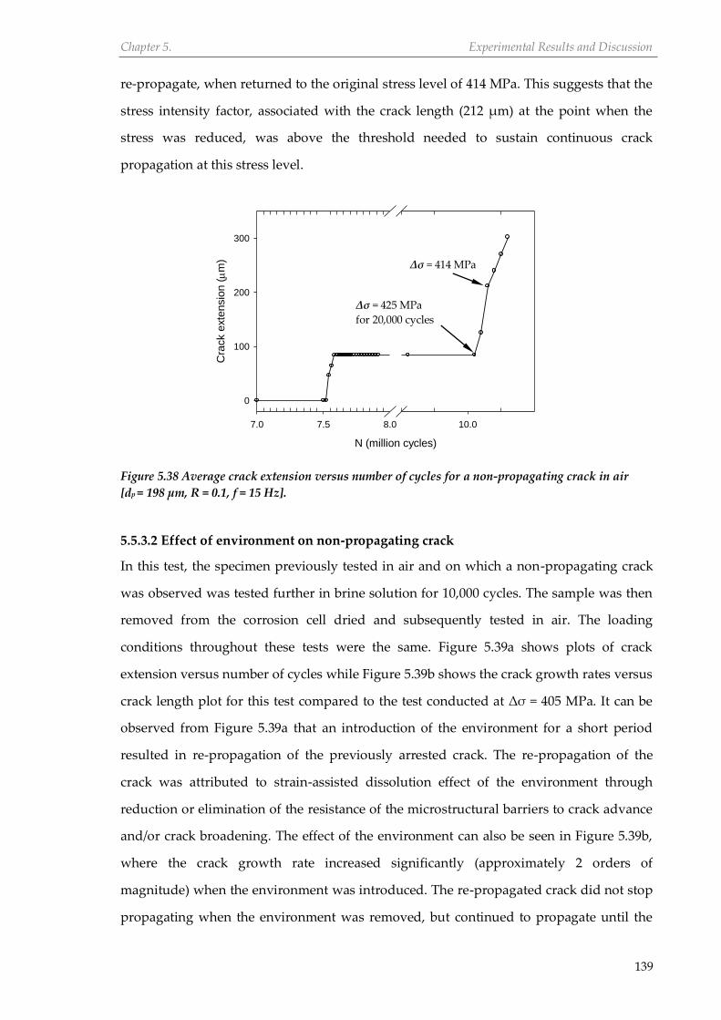
Chapter 5. Experimental Results and Discussion
139
re-propagate, when returned to the original stress level of 414 MPa. This suggests that the
stress intensity factor, associated with the crack length (212 µm) at the point when the
stress was reduced, was above the threshold needed to sustain continuous crack
propagation at this stress level.
N (million cycles)
7.0 7.5 8.0 10.0
Cra
ck e
xte
nsio
n (
m)
0
100
200
300
Figure 5.38 Average crack extension versus number of cycles for a non-propagating crack in air
[dp = 198 µm, R = 0.1, f = 15 Hz].
5.5.3.2 Effect of environment on non-propagating crack
In this test, the specimen previously tested in air and on which a non-propagating crack
was observed was tested further in brine solution for 10,000 cycles. The sample was then
removed from the corrosion cell dried and subsequently tested in air. The loading
conditions throughout these tests were the same. Figure 5.39a shows plots of crack
extension versus number of cycles while Figure 5.39b shows the crack growth rates versus
crack length plot for this test compared to the test conducted at Δσ = 405 MPa. It can be
observed from Figure 5.39a that an introduction of the environment for a short period
resulted in re-propagation of the previously arrested crack. The re-propagation of the
crack was attributed to strain-assisted dissolution effect of the environment through
reduction or elimination of the resistance of the microstructural barriers to crack advance
and/or crack broadening. The effect of the environment can also be seen in Figure 5.39b,
where the crack growth rate increased significantly (approximately 2 orders of
magnitude) when the environment was introduced. The re-propagated crack did not stop
propagating when the environment was removed, but continued to propagate until the
Δσ = 425 MPa
for 20,000 cycles
Δσ = 414 MPa

Chapter 5. Experimental Results and Discussion
140
specimen failed. However, the crack growth rates decreased to values marginally lower
than those observed from tests carried out at a higher stress level (Δσ = 405 MPa). It has
been suggested that continued crack propagation in air is only possible when the length
of a crack is the same as or greater than a threshold crack length [89]. These results
suggest that the environmental was instrumental in promoting growth of the crack from
pits beyond barriers inherent within the microstructure. The continued crack propagation
after removal of the environment suggests that the role of the environment in crack
growth is important in the early stages when the cracks are short.
N (million cycles)
8.0 10.0
Cra
ck length
(
m)
0
200
400
600
800
1000
Crack length (m)
101 102 103
Cra
ck g
row
th r
ate
(m
/cyc
le)
10-10
10-9
10-8
10-7
= 382.5 MPa
= 405 MPa
Figure 5.39 (a) Crack extension versus number of cycles for a non-propagating crack in air
subjected temporarily to an aggressive environment, (b) crack growth rates versus crack length for
data in (a) [dp = 274 µm, ARp = 0.82].
Introduction of
environment
Removal of
environment
Crack initiation
Crack arrest
Introduction of
environment
Removal of
environment
(a)
(b)

Chapter 5. Experimental Results and Discussion
141
5.5.4 Crack propagation lifetimes
5.5.4.1 Single pits – fatigue tested in air and corrosion fatigue
Figures 5.40a shows that the overall propagation lifetime of the cracks emanating from
pits is mainly influenced by the test environment and stress level, whereas the pit size
appears to have no significant effect. Where cracks did not initiate, notably in air, 𝑁𝑝 is
zero hence, no plots were shown for this cases. Generally, 𝑁𝑝 in brine solution are lower
than in air for all stress levels, and increase with decrease in stress levels for both
environments. For a given stress level, there seems to be no apparent differences between
the propagation lifetime observed for different pit sizes. The propagation lifetimes were
plotted as a fraction of fatigue life as shown in Figure 5.40b. The notable observation here
is that, the propagation life ratios are generally less than 40% of the fatigue lives, which
indicates the fatigue behaviour is still dominated by the crack initiation stage in both air
and corrosion fatigue conditions. However, the percentage crack propagation lives
appears to be greater in corrosion fatigue than in air and they generally decrease with
reduction in pit size at a given stress level. This is expected since the fatigue behaviour is
dominated by crack initiation lives, which were earlier shown to increase with decrease in
pit size and are lower (as a fraction of the total fatigue lives) in the brine solution than in
air.
Stress range (MPa)
0 20 40 60 80 100
Cra
ck p
ropagation life, N
p (
cyc
les)
104
105
106
dp = 140 mm (ARp = 0.52)
dp = 200 mm (ARp = 0.68)
dp = 270 mm (ARp = 0.82)
450 427.5405
(a)

Chapter 5. Experimental Results and Discussion
142
Stress range (MPa)
0 20 40 60 80 100
Np/N
f (%
)
0
10
20
30
40
50
dp = 140 m (ARp = 0.52)
dp = 200 m (ARp = 0.68)
dp = 270 m (ARp = 0.82)
450 427.5405
Figure 5.40 Comparison between crack propagation lives in air and brine solution for different
stress levels and pit sizes as function of (a) number of cycles and (b) fraction of total lifetime.
[Plain bars = Air; Hatched pattern bars = Corrosion fatigue]. Arrows indicate that Np & Np/Nf ≈ 0.
5.5.4.2 Double pits – fatigue tested in air
Changes in fatigue behaviour from initiation-dominant to propagation-dominant
behaviour was investigated by plotting propagation lifetimes (𝑁𝑝) and fatigue lifetimes
(𝑁𝑓) as a function of separation distance between the pits (Figures 5.41 – 5.42). 𝑁𝑝 is given
by 𝑁𝑝 = 𝑁𝑓 - 𝑁𝑖. Unlike crack initiation lifetime results, a large scatter in 𝑁𝑝 was observed,
with only a marginal trend, notably that 𝑁𝑝 decreased with increase in separation distance
(see trend lines in Figure 5.41a). Furthermore, for a constant separation distance, whereas
𝑁𝑝 were generally higher at lower stresses, no dependency on pit size was observed. The
scatter in the data is thought to be due to factors which include crack coalescence and
crack initiation from only one or both pits. For instance, at a given stress level and
separation distance, crack coalescence can shorten crack propagation life compared to
when there is no coalescence.
To explain the decrease in 𝑁𝑝 with increasing separation distance, the crack size as a
function of separation distance was considered. At a given stress level, consider two
specimens A and B containing double pits with the same depth but different edge-to-edge
distances 𝑠𝑒𝑒,𝐴 and 𝑠𝑒𝑒,𝐵 respectively where 𝑠𝑒𝑒,𝐴 < 𝑠𝑒𝑒,𝐵. Due to the greater separation
(b)

Chapter 5. Experimental Results and Discussion
143
distance, the effective size and the SIF associated with a crack propagating in the region
separating both pits in specimen B will be greater than in specimen A.
Center-to-center distance (m)
600 800 1000
Cra
ck p
ropagation life,
Np (
'000 c
ycle
s)
200
300
400
500
ARp = 0.68 ( = 405 MPa)
ARp = 0.82 ( = 405 MPa)
ARp = 0.68 ( = 427.5 MPa)
ARp = 0.82 ( = 427.5 MPa)
Center-to-center distance (m)
600 800 1000 1200 1400
Np/N
f (%
)
0
20
40
60
80
100
ARp = 0.68 ( = 405 MPa)
ARp = 0.82 ( = 405 MPa)
ARp = 0.68 ( = 427.5 MPa)
ARp = 0.82 ( = 427.5 MPa)
Figure 5.41 Crack propagation lives versus centre-to-centre distance between two pits as a
function of pit size and applied stress, plotted in terms of (a) number of cycles and (b) fraction
fatigue life.
Consequently, the growth rate will be faster in specimen B and hence, generating a
shorter Np. The SIF is also a function of applied stress for a given crack size, which implies
that increasing the applied stress range will result in faster propagation rate and shorter
𝑁𝑝. This explains why, for the same separation distance, propagation lives tend to be
shorter for tests carried out at Δσ = 427.5 MPa compared to those at 405 MPa. The
(a)
(b)

Chapter 5. Experimental Results and Discussion
144
independency observed between pit size and 𝑁𝑝 also suggests that the role of the former
in the fatigue behaviour in the presence of multiple pits may be limited mainly to the
crack initiation stage.
Re-plotting the data in terms of percentage propagation lifetimes (𝑁𝑝 𝑁𝑓⁄ ) (Figure 5.41b),
as expected, shows a reverse of the trend observed in the percentage crack initiation
(𝑁𝑖 𝑁𝑓⁄ ). For all the stress levels and pit sizes, 𝑁𝑝 𝑁𝑓⁄ generally decreased with increasing
separation distance. Comparison of Figures 5.20b and 5.41b shows that for the pits closest
together, where the mechanical interaction of the pits is expected to be greatest, the
(𝑁𝑖 𝑁𝑓⁄ ) is lowest while the (𝑁𝑝 𝑁𝑓⁄ ) is highest, indicating that fatigue behaviour is
propagation-dominant. As the separation distance increases, the interaction between the
pits reduces and thus, initiation of cracks becomes less likely. Consequently, (𝑁𝑖 𝑁𝑓⁄ )
increases and the fatigue life increasingly becomes initiation-dominant.
The relationship between the overall fatigue lives and separation distance is shown in
Figure 5.42 where fatigue lives can be seen to decrease with decrease in separation
distance at all stress levels and pit sizes. This is consistent with previous observation that
fatigue behaviour of double pitted samples, in air, is controlled by the crack initiation
stage when there is mechanical interaction between the pits.
Center-to-center distance (m)
600 800 1000 1200 1400
Fa
tig
ue
life
, N
f (c
ycle
s)
105
106
107
ARp = 0.68 ( = 405 MPa)
ARp = 0.82 ( = 405 MPa)
ARp = 0.68 ( = 427.5 MPa)
ARp = 0.82 ( = 427.5 MPa)
Figure 5.42 Fatigue lives versus separation distance between two pits as a function of pit size and
applied stress. Horizontal lines represent corresponding values for single pits.
ARp = 0.68
Δσ = 405 MPa
ARp = 0.82
Δσ = 427.5 MPa
ARp = 0.68
Δσ = 427.5 MPa
ARp = 0.82
Δσ = 405 MPa
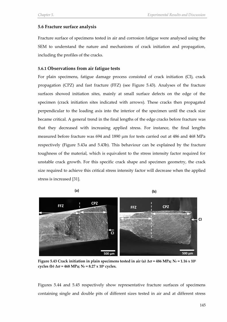
Chapter 5. Experimental Results and Discussion
145
5.6 Fracture surface analysis
Fracture surface of specimens tested in air and corrosion fatigue were analysed using the
SEM to understand the nature and mechanisms of crack initiation and propagation,
including the profiles of the cracks.
5.6.1 Observations from air fatigue tests
For plain specimens, fatigue damage process consisted of crack initiation (CI), crack
propagation (CPZ) and fast fracture (FFZ) (see Figure 5.43). Analyses of the fracture
surfaces showed initiation sites, mainly at small surface defects on the edge of the
specimen (crack initiation sites indicated with arrows). These cracks then propagated
perpendicular to the loading axis into the interior of the specimen until the crack size
became critical. A general trend in the final lengths of the edge cracks before fracture was
that they decreased with increasing applied stress. For instance, the final lengths
measured before fracture was 694 and 1890 µm for tests carried out at 486 and 468 MPa
respectively (Figure 5.43a and 5.43b). This behaviour can be explained by the fracture
toughness of the material, which is equivalent to the stress intensity factor required for
unstable crack growth. For this specific crack shape and specimen geometry, the crack
size required to achieve this critical stress intensity factor will decrease when the applied
stress is increased [31].
Figure 5.43 Crack initiation in plain specimens tested in air (a) Δσ = 486 MPa; Nf = 1.16 x 10⁵
cycles (b) Δσ = 468 MPa; Nf = 8.27 x 10⁵ cycles.
Figures 5.44 and 5.45 respectively show representative fracture surfaces of specimens
containing single and double pits of different sizes tested in air and at different stress
500 µm 500 µm
(a) (b)
CPZ FFZ
CI
CI
CPZ FFZ

Chapter 5. Experimental Results and Discussion
146
levels. Fractographic analyses showed that the fatigue damage process proceeded
through the following stages: crack initiation (CI), crack propagation (CPZ) and fast
fracture (FFZ). These stages, shown in Figure 5.44a, were observed on all fractured
specimens. Some of the samples were fractured in liquid nitrogen to reveal the shape of
the cracks, which was found to be approximately hemispherical. High magnification
analyses suggest that cracks initiated predominantly from the pit mouth. On the single-
pitted specimens, the cracks that initiated at the pit mouth propagated radially outwards
and likely coalesced at some point during the propagation stage. A notable observation at
the bottom of the single pits was the differences in the propagation plane of the two
cracks (Figures 5.44b and 5.44d). Differences in crack planes indicate that there were two
different cracks. This was not observed in any of the double-pitted specimens since either
only a single initiated crack or two cracks coalesced into a dominant crack and then
propagated to failure during the fatigue life of the double-pitted specimens. Figure 5.45d
shows a typical fracture surface of specimen on which the separation distance between
the double pits was above the threshold distance for a particular pit size and stress level.
The fracture surface and crack profile were similar to those of the single-pitted specimens
except the presence of the second pit, which seems not to have any effect on the crack
front. This corroborates the observations made during crack propagation monitoring,
which showed that the double pits seemed to behave as single pits when their separation
distance is above a threshold value.
500 µm 500 µm
(a) (b)
CPZ
FFZ
CI CI

Chapter 5. Experimental Results and Discussion
147
Figure 5.44 SEM images of fracture surface of single-pitted specimens in air. (a) Δσ = 427.5 MPa, dp
= 202 µm, Ni = 0.958 Nf, Nf = 44.97 x 10⁵ cycles; (b) Δσ = 405 MPa, dp = 265 µm, Ni = 0.965 Nf, Nf =
52.05 x 10⁵ cycles; (c) Δσ = 450 MPa, dp = 267 µm, Ni = 0.707Nf = 5.35 x 10⁵ cycles; (d) Δσ = 450 MPa,
dp = 204 µm, Ni = 0.889Nf, Nf = 15.13 x 10⁵ cycles.
Figure 5.45 SEM images of fracture surface of double-pitted specimens in air (a) Δσ = 427.5 MPa,
dp(1) = 268 µm, dp(2) = 274 µm, scc = 776 µm, Ni = 0.7 x 10⁵ cycles, Nf = 3.85 x 10⁵ cycles; (b) Δσ = 405
MPa, dp(1) = 265 µm, dp(2) = 273 µm, scc = 877 µm, Ni = 7.96 x 10⁵ cycles, Nf = 1.196 x 10⁶ cycles; (c) Δσ =
405 MPa, dp(1) = 197 µm, dp(2) = 206 µm, scc = 782 µm, Ni = 1.652 x 10⁶ cycles, Nf = 2.112 x 10⁶ cycles;
(d) Δσ = 427.5 MPa, dp(1) = 203 µm, dp(2) = 195 µm, scc = 1066 µm, Ni = 4.485 x 10⁶ cycles, Nf = 4.795 x
106 cycles. Crack initiation sites are indicated with arrows.
500 µm 500 µm
500 µm 500 µm
500 µm 200 µm
(c) (d)
(a) (b)
(c) (d)

Chapter 5. Experimental Results and Discussion
148
5.6.2 Observations from corrosion fatigue tests
Figures 5.46 shows representative fracture surfaces of single-pitted specimens tested in
brine at different stress levels. Fractographic analyses showed that the corrosion fatigue
damage process also proceeded through crack initiation (CI), crack propagation (CPZ)
and fast fracture (FFZ) (Figure 5.46a and 5.46b). Several white lines emanating from the
pit and the different crack planes observed on the entire test specimens especially at the
pit bottom suggests multiple crack initiation sites (Figure 5.46c and 5.46d). This supports
the observations made during crack growth monitoring where multiple cracks initiated
from the pit bottom. The crack shapes in the aggressive environment were also found to
be approximately hemispherical (see crack depth and width measurement on Figure
5.46a).
Figure 5.46 SEM images of fracture surface of single-pitted specimens in brine. (a&c) Δσ = 427.5
MPa, dp = 266 µm, ARp = 0.82, Ni = 2.36 x 10⁵ cycles, Nf = 3.13 x 10⁵ cycles; (b) Δσ = 450 MPa, dp = 197
µm, ARp = 0.68, Ni = 1.95 x 10⁵ cycles, Nf = 2.44 x 10⁵ cycles; (d) Δσ = 405 MPa, dp = 265 µm, ARp =
0.81, Ni = 2.92 x 10⁵ cycles, Nf = 4.19 x 10⁵ cycles.
200 µm 200 µm
500 µm 500 µm
(a) (b)
(c) (d)
CPZ
FFZ

Chapter 5. Experimental Results and Discussion
149
5.6.3 Aspect ratio of cracks emanating from pits
The replica method for crack monitoring only allows for measurement of the surface
length of cracks; hence, it was impossible to measure the depth of the cracks. However, if
the aspect ratio of a crack is known, it will be possible to make a realistic prediction of its
depth from a known surface length. The aspect ratio, 𝐴𝑅𝑐 , of a surface crack was
evaluated as the ratio of crack depth, dc, to the crack surface length (including the pit
width), ac. The crack shapes of specimens tested in air and brine solution were analysed
by measuring the depth and width of the crack front from the fracture surface of non-
failed specimens, broken in liquid nitrogen. Figures 5.44a, 5.45a and 5.46a show
representative fractographs of the crack shapes in air (single and double pits) and
corrosion fatigue. Irrespective of the test environment, stress level, pit size and number of
pits on the surface of the specimen, the surface cracks appear to have semi-elliptical
shapes. Table 5.7 shows the dimensions and aspect ratios of cracks. It is noted that these
images were taken at N > 0.7Nf, which only represents the crack shapes in the latter stages
of cracking. The different crack planes together with results from in-air crack initiation
behaviour from pit mouth suggest that the cracks in the early stages of cracking were
corner cracks. These corner cracks grew separately on both sides of the pit until they were
at or beyond the root of the pit where they merge into a single semi-elliptical crack.
Table 5.7 Typical aspect ratios of surface cracks emanating from pits in air and corrosion fatigue.
Specimen
No
Stress range
(MPa)
Pit depth
(µm)
Pit aspect
ratio
Crack depth
(µm)
Crack width
(µm)
Crack aspect
ratio
SNAF64 427.5 198 0.68 1020 2528 0.81
SNAF51 450 141 0.52 793 1650 0.96
SN3PAF 427.5 268 0.82 1022 2460 0.83
SNAF39 405 272 0.82 1325 3117 0.85
SNCF59 405 265 0.81 1230 3060 0.80
SNCF61 450 197 0.68 1150 2860 0.80
SNCF84 450 141 0.52 752 1714 0.88
SNCF85 450 271 0.82 1239 2951 0.84
5.6.4 Mechanisms of fatigue damage
For all test types of carried out, the prevalent mechanisms of damage during the fatigue
damage process were identified. Figure 5.47 shows representative low and high
magnifications of morphology of fracture surfaces for tests carried out in air and the brine

Chapter 5. Experimental Results and Discussion
150
solution. In the crack propagation zone, ductile fatigue striations, which are characteristic
of sub-critical transgranular crack growth, were observed in air (Figures 5.47a – 5.47b).
Figure 5.47 Representative morphology of fracture surfaces for tests carried out (a & b) in air
showing fatigue striations, (c & d) in air showing dimple rupture and micro-void coalescence and
(e & f) in brine showing oxide products.
A generally accepted model for rationalizing striation formation in ductile materials is the
repetitive plastic blunting and re-sharpening occurring at the crack tip [288]. Figures 5.47c
10 µm
10 µm 1 µm
1 µm
1 µm 10 µm
(
a
)
(a) (b)
(c) (d)
(e) (f)

Chapter 5. Experimental Results and Discussion
151
– 5.47d show the fast fracture region where damage was by ductile tearing through
dimple rupture and coalescence of microvoids in air and the test environment. In the
aggressive environment, transgranular fracture mode and pronounced oxide products
were found on the fracture surface, which typically indicates anodic dissolution during
crack propagation (Figures 5.47e – 5.47f). On one hand, anodic dissolution process can
lead to enhanced crack growth rates and shorter fatigue lives [16, 122, 289]. On the other
hand, the wedge effect of oxide products can result in oxide-induced crack closure
thereby reducing the crack growth rates [170, 290, 291]
5.7 Stress-life (S-N) curves
The fatigue endurance lifetime (Nf) of pre-pitted specimens in air and brine solution were
obtained from the summation of the crack initiation (Ni) and crack propagation (Np)
stages. The relationship between stress range and cycles to failure for the plain specimens
in air for this material is given in Figure 5.48. It shows that a plain fatigue limit stress
range (450 MPa) exists below which specimens did not fail under these loading conditions
Testing of single and double-pitted specimens in air and corrosion fatigue was carried out
at stress ranges below the plain fatigue limit. Figure 5.48 shows that fatigue lives
generally increased with decrease in stress range in air irrespective of pit size. The S-N
curves for the pitted specimens relative to that of the plain specimen show that fatigue
limit decreased with increasing pit size. Since the applied stresses are below the plain
specimen fatigue limit, these results suggest that the pit acted as a strain localisation site
where cracks initiated, which otherwise, would not initiate in the absence of the pit. The
curves also show that limiting stresses are associated with each pit size at which
specimens did not fail irrespective of whether cracks initiated from the pit or not. The
estimated limiting stress range corresponding to each pit size is given in Table 5.8. The
differences between the minimum stress range at which the specimen did not fail
(including those with non-propagating cracks) and the maximum stress range at which
failure occurred was taken to be the uncertainty in fatigue limit values. The table shows
that a greater pit size generally leads to a lower fatigue limit.

Chapter 5. Experimental Results and Discussion
152
Figure 5.48 S-N endurance curves for plain and single-pitted specimens in air.
Table 5.8 Fatigue limit of X65 steel with and without pits (R = 0.1, f = 15 Hz)
Pit depth (µm) Aspect ratio Fatigue limit (MPa)
Plain - 450
140 0.52 436.5 ± 13.5
200 0.68 414 ± 13.5
270 0.82 382.5 ± 22.5
The endurance curves for double-pitted specimens were also compared with those of
plain and single-pitted specimens. Ideally, double pits, which have different sizes but
identical separation distances can only be compared at the same stress level on the S-N
curve. As discussed previously, the limitation of the experiment procedure employed for
generating the double pits meant that the separation distance between pits of the different
sizes varied, although not significantly (7% maximum). The effect of double pits on
fatigue lives is depicted in Figure 5.49. A shift of the S-N curves to the left, compared to
the single pits, indicates a further reduction in fatigue life when double pits are present;
even for the same stress level and pit sizes. However, the extent of the reduction depends
on the separation distances between the pits. Irrespective of pit size, fatigue lives
generally become shorter with decreasing separation distance between pits and with
increasing stress level. Furthermore, for a given stress level, fatigue lives are shorter when
the pit size increases. It is interesting to note that the slopes of the S-N curves for double

Chapter 5. Experimental Results and Discussion
153
pits with similar separation distances appear to be similar irrespective of pit size and that
the slopes of the curves when see is 200 µm is similar to the slopes of corresponding single
pit sizes. The latter observation suggests that there may be endurance limits that will
correspond to a fatigue life of 107 cycles but will be lower than that associated with that of
single pit.
Figure 5.50 shows the results for the tests conducted in brine solution, plotted with
reference to air tests. It can be observed that fatigue lives are shorter in the brine solution
compared to air. Fatigue lives were also found to increase with decreasing stress range
and decreasing pit size. A progressive decrease in the S-N curve compared to
corresponding in-air plots show the effect of the aggressive environment in the form of a
significant degradation in fatigue performance. Three additional tests (also plotted on the
corrosion fatigue S-N curve) were carried out for each pit size at a lower stress range (350
MPa) to evaluate the possibility of an endurance limit in corrosion fatigue. This chosen
stress was the lowest possible given the available testing time. The trend in the curves for
each pit size suggests a reduction/elimination of the fatigue limit under corrosion fatigue
conditions for all pit sizes.
Figure 5.49 S-N endurance curves for plain, single-pitted and double-pitted specimens in air.
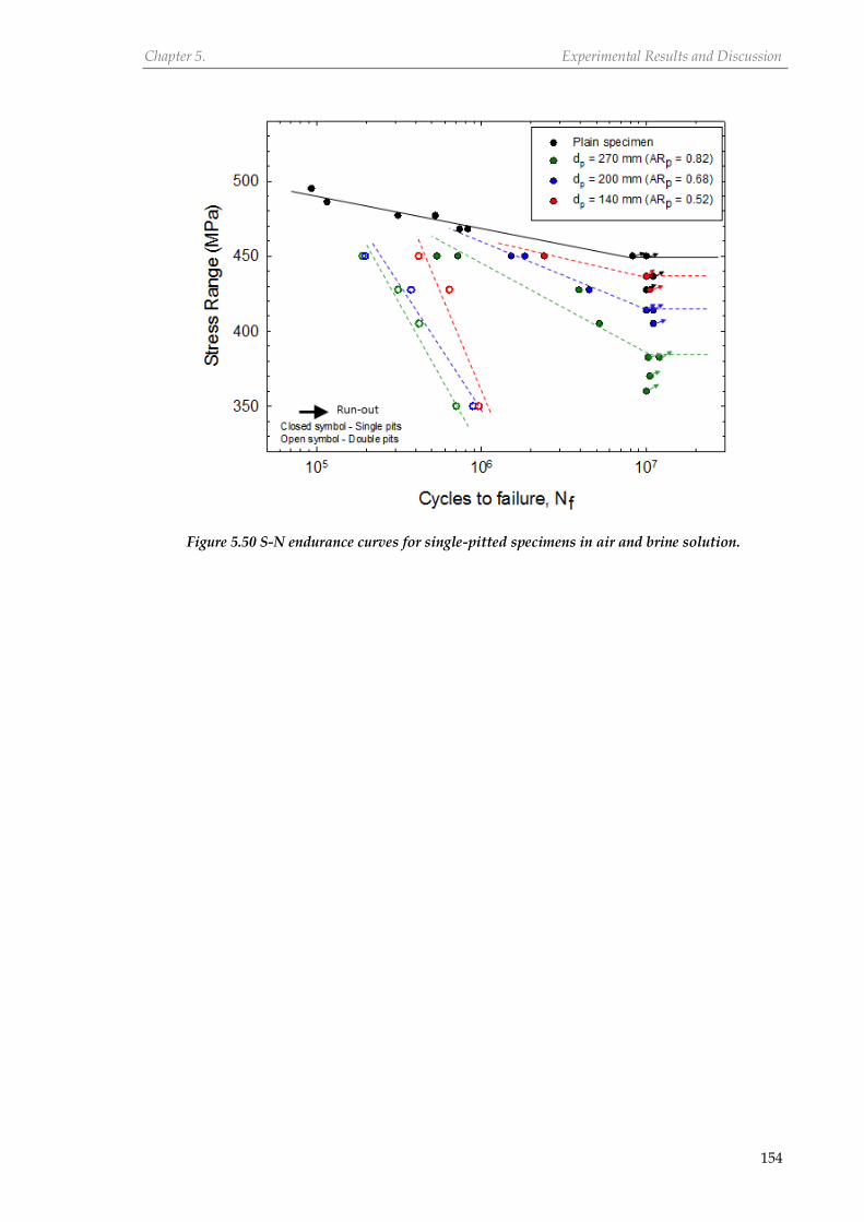
Chapter 5. Experimental Results and Discussion
154
Figure 5.50 S-N endurance curves for single-pitted specimens in air and brine solution.

Chapter 6
Finite Element Analysis
Results and Discussion

Chapter 6. Finite Element Analysis Results and Discussion
156
6.1 Introduction
In many metal-environment systems where corrosion pits are precursors to fatigue cracks,
understanding the conditions that facilitate cracking from corrosion pits is important in
order to predict pit-to-crack transition. As discussed in Chapter 5, the present research
study showed that corrosion pits are the preferred sites for crack nucleation and that the
preferred sites around pits where crack initiate and pit-to-crack transition lifetimes
depend on pit characteristics (pit depth, pit aspect ratio and proximity between pits),
stress level, operating environment and interactions between them. These results
demonstrate that the conditions required for transition depend not only on
electrochemical, but also on mechanical factors. Although the latter, through strain-
assisted dissolution, can influence corrosion kinetics to a large extent, its primary
influence is through stress and strain localization effect, which can induce plasticity in the
vicinity of the pit and thereby result in cracking. Therefore, the relationship between these
mechanical factors, the size, shape and proximity of pits and applied stress must be
appropriately understood for accurate pit-to-crack transition modelling. Although stress
and strain localization effectively increases the maximum stress and strain on a
component, the mechanical response cannot be determined solely by the maximum stress
(elastic stress concentration factor) or strain (elastic strain concentration factor) around the
pit. Other factors such as stress/strain distribution profile (elastic-plastic behaviour), cyclic
loads and material properties must be considered. In the present study, these phenomena
were investigated in detail with a view to gaining greater insight into the mechanics-
based conditions that facilitate emergence of cracks from pits. Based on the results
derived during this study, plausible explanations are postulated to support experimental
observations relating to crack initiation sites and pit-to-crack transition lifetimes.
A detailed FEA was carried out to evaluate the distribution of stress and strain around
‘artificial’ and ‘ideal’ pits of varying sizes, shapes and separation distances, subject to a
remote tensile loads. The artificial pits are those pits obtained experimentally using the
micro-capillary cell, while the ideal pits are idealizations of the experimental pits as
elliptically shaped 3-D models having a smooth surface (see Section 4.4 for description of
procedure). The models of the artificial pits were obtained from 3-D scans by employing a

Chapter 6. Finite Element Analysis Results and Discussion
157
3-D confocal microscope. In general, each or both types of 3-D models were analysed
depending on computational time limitations. The results from the present investigation
have been divided into the following categories:
1. Evaluation of changes in pattern of distribution of stress and strain as a result of
changes in pit sizes due to pit growth.
2. Assessment of the correlations between localisation of crack initiation sites, pit
size, proximity between pits, applied stress and general pit-to-crack transition
behaviour.
6.2 Mesh convergence study
The results presented in Figure 6.1 show that the stress concentration factor converged
after a finer mesh element size of 10 and 5 µm for the ideal and artificial pits respectively.
Therefore, in the finer and coarse regions respectively, element sizes of 10 and 100 µm
were employed for ideal pits and 5 and 100 µm for artificial pits. Depending on pit
characteristics, mesh density around the pits will change to ensure consistency in the size
of elements created around a pit but the levels of accuracy should be similar.
Finer mesh size (m)
1 10 100
Str
ess c
oncentr
ation facto
r
1.2
1.4
1.6
1.8
2.0Ideal pit
Artificial pit
Figure 6.1 Variations of stress concentration factor with finer mesh size.
6.3 Model validation
Figure 6.2 shows that predictions from the FE model are in good agreement with those
obtained empirically. A satisfactory agreement can also be observed in Figure 6.3, which

Chapter 6. Finite Element Analysis Results and Discussion
158
compares the surface strain predictions from the FEA of an artificial pit with those
obtained from DIC experiment. In general, it can be concluded that the FE models of the
ideal and artificial pits are reasonably valid for conducting further investigations on stress
and strain distributions around corrosion pits.
Aspect Ratio (a/c)
0.0 0.5 1.0 1.5 2.0
Str
ess c
oncentr
ation facto
r (K
)
1.0
1.5
2.0
2.5
Str
ain
concentr
ation facto
r (K
)
1.0
1.5
2.0
2.5
Kt - Empirical
K - FEA
K - FEA
Kt = [1 + 6.6(a/2c)]
[1 + 2(a/2c)]
Figure 6.2 Comparison between empirical and FEA model predictions of stress and strain
concentration factors for various pit aspect ratios.
Ref. [1]
(a) (b)
DIC FEA
500 µm
500 µm

Chapter 6. Finite Element Analysis Results and Discussion
159
Figure 6.3 Validation of FEA model predictions and surface strain maps obtained from DIC
measurements for an artificial pit that is 440 µm deep pit and with aspect ratio of 1.1 loaded to
470 MPa in (a & b) and 596 MPa in (c & d). Loading direction is from top to bottom.
6.4 Changes in stress and strain distribution due to pit growth
Since modelling of pit growth in a continuous mode is very challenging, a discretized
approach was adopted in which pit sizes at discrete time intervals were modelled to
simulate pit growth. Thus the influence of time-dependent increasing pit size (pit growth)
on localization of stress and strain was investigated by evaluating the distribution of
stress and strain around pits of different depths and aspect ratios. The modelled pit sizes,
which were obtained from pit growth experiments, were chosen to simulate the
instantaneous pit size at different time periods ranging from 3600 to 28800 seconds. The 3-
D models of fatigue specimens containing the pits were loaded to stresses between 425
and 500 MPa (similar to those applied during experiments). Table 6.1 summarises the
experimental average values of the characteristics of the pits that were modelled.
Table 6.1 Summary of characteristics of pits obtained experimentally.
Time (s) Pit depth (µm) Pit aspect ratio
3600 112 0.44
7200 140 0.52
14400 200 0.68
21600 240 0.78
28800 270 0.82
(d) (c)
DIC FEA
500 µm 500 µm

Chapter 6. Finite Element Analysis Results and Discussion
160
Figure 6.4 shows representative 3-D distribution of stress and total strain in a modelled
pre-pitted flat fatigue specimen containing a 270 µm pit and loaded to 500 MPa. It can be
observed that the critical region where stress and strain are localized is generally in the
vicinity of the pit in the direction perpendicular to the loading axis. This agrees with
experimental observations where cracks were found to initiate from the pits in pre-pitted
specimens due to strain localisation.
Figure 6.4 Representative contour plots showing maximum principal stress distribution (a) and
maximum principal strain distribution (b) around a 270 µm pit in a flat fatigue specimen loaded to
500 MPa.
The localised stresses and strains evaluated as maximum values of the principal stress,
principal strain and plastic strain for each pit size at different stress levels are compared
graphically in Figure 6.5. The corresponding relations of the localised stresses with yield
stress of the material and of localised strains with yield strain (equivalent total strain at
yield point) and nominal strain (elastic strain equivalent to the elastic nominal stress) are
shown in Figures 6.5a, 6.5b and 6.5c respectively. In general, local stresses and strains are
higher than the yield stress and yield strain of the material indicating localised plasticity.
(b)
(a)

Chapter 6. Finite Element Analysis Results and Discussion
161
The localised stress and strain increased with increasing pit depth, pit aspect ratio and
applied stress. Similar findings have been reported in previous studies on the mechanical
effect of pits in structural components [201, 230, 234]. By way of extension, since the
investigated pit characteristics are time-dependent, the results also suggest that the
localised resulting from pits increase with time. This will further intensify these effects as
time increases. An interpretation of this is that a growing pit with increasing size may be
inducing corresponding increasing levels of stress and strain with time, a behaviour
which can be perceived as the pit inducing local dynamic strain. However, it is
conceivable that this intensification would not normally continue endlessly since the
conditions for crack nucleation will be determined by a combination of a critical pit size
and mechanical and electrochemical factors. As dynamic strain, notably dynamic plastic
strain is recognized to result in the nucleation of cracks, it is thought that the plastic strain
rate resulting from the growing pit would increase.
From the perspective of cracking, it has been recognised that localised plastic flow is the
main driving force for fatigue crack nucleation [31, 292, 293]. Based on this premise, the
results shown in Figures 6.5b and 6.5c would suggest that the conditions required for
crack nucleation will be more favoured at relatively larger pit sizes and higher applied
nominal stresses for which local total and plastic strains are relatively higher. In order
words, cracks will tend to initiate more readily i.e. shorter period for crack nucleation, at
relatively larger pit sizes and higher stress levels. This agrees well with experimental
observations in air and aggressive environment reported in Chapter 5 where it was
shown that pit-to-crack transition lifetimes decreased with increase in pit depth, pit aspect
ratio and stress level (see Section 5.5.1.3).
To explain the nucleation of cracks from the pit mouth, the distribution of principal stress,
principal strain and plastic strain in the pit region is examined further by comparing the
cross section in the pit region viewed perpendicular to loading for 112 and 270 µm pits
representing shallow (early stages of pitting) and deep pits (latter stages of pitting).
Representative results for 425 MPa and 500 MPa are presented in Figures 6.6 and 6.7
respectively. It can be observed that stress distributions appears to be uniform around the
pits although the stress tends to be more concentrated at the pit base at relatively higher
stresses and larger pit size (Figure 6.6a&b and 6.7a&b).

Chapter 6. Finite Element Analysis Results and Discussion
162
Nominal stress (MPa)
0 10 20 30 40 50
Local str
ess (
MP
a)
520
560
600
640
112 m
140 m
200 m
240 m
270 m
425 450 475 500
Nominal stress (MPa)
0 10 20 30 40 50
Local to
tal str
ain
(%
)
0.2
0.3
0.4
0.5
0.6112 m
140 m
200 m
240 m
270 m
425 450 475 500
Nominal stress (MPa)
0 10 20 30 40 50
Local pla
stic s
train
(%
)
0.0
0.1
0.2
0.3
0.4112 m
140 m
200 m
240 m
270 m
425 450 475 500
Figure 6.5 Summary of maximum values of (a) local maximum stress (b) local maximum total
strain and (c) local maximum plastic strain for pits of increasing.
Yield stress
Yield strain
Nominal strain
(c)
(a)
(b)

Chapter 6. Finite Element Analysis Results and Discussion
163
Figure 6.6 Comparison between stress distribution (a,b), total strain distribution (c,d), and plastic
strain distribution (e,f) between a 112 µm (a,c,e) and 270 µm (b,d,f) pit loaded at 425 MPa and
viewed perpendicular to the loading axis.
Pit depth = 112 µm, Aspect ratio = 0.44 Pit depth = 270 µm, Aspect ratio = 0.82
(a)
(c) (d)
(e) (f)
(b)

Chapter 6. Finite Element Analysis Results and Discussion
164
Figure 6.7 Comparison between stress distribution (a,b), total strain distribution (c,d), and plastic
strain distribution (e,f) between a 112 µm (a,c,e) and 270 µm (b,d,f) pit loaded at 500 MPa and
viewed perpendicular to the loading axis.
Pit depth = 112 µm, Aspect ratio = 0.44 Pit depth = 270 µm, Aspect ratio = 0.82
(a) (b)
(f) (e)
(d) (c)

Chapter 6. Finite Element Analysis Results and Discussion
165
Qualitative results of inspection of the area around the pit surface (Figure 6.8) at different
load levels shows that the maximum stresses occurred at the pit bottom (see principal
stress section of Table 6.2). Figure 6.6c&e and 6.7c&e show that the distributions of total
strains and plastic strains appear to be concentrated at the base for the shallow pit but
tend to shift away from the base to the region between the pit mouth and pit base. The
maximum strains occurred at different regions depending on pit size (see principal strain
and plastic strain sections of Table 6.2). Whereas the maximum strains are predominantly
located at the base at pit depths up to 200 µm at all stress levels, they are shifted away
from the base to region closer to the pit mouth (point ‘B’ in Figure 6.8) at relatively larger
pit depths. However, further analysis of these deeper pits shows that the differences
between the values at regions B and E (pit base) is generally less than 1%. Therefore, it is
concluded that the strain distribution within the pit are largely uniform from the mouth
to the base of the pit and not concentrated at the pit mouth.
Figure 6.8 Schematic of critical areas of stress and strain concentration around a pit.
Table 6.2 Summary of locations of maximum stresses and strains around pits of various sizes
loaded to different stress levels. (Refer to Figure 6.8—for location of letters A to E).
Principal stress
Pit depth (µm) 425 MPa 450 MPa 475 MPa 500 MPa
112 E E E E
140 E E E E
200 E E E E
240 E E E E
270 E E E E
Principal (total) strain
Pit depth (µm) 425 MPa 450 MPa 475 MPa 500 MPa
112 E E E E
140 E E E E
200 E E E E
240 E B B B
270 B B B B
A
B
C D
E

Chapter 6. Finite Element Analysis Results and Discussion
166
Plastic strain
Pit depth (µm) 425 MPa 450 MPa 475 MPa 500 MPa
112 E E E E
140 E E E E
200 E E E E
240 E D B B
270 B B B B
Figure 6.9 shows comparisons between the maximum values of principal stresses and
strains obtained at the pit mouth (point ‘A’ in Figure 6.8) and pit bottom (point ‘E’ in
Figure 6.8). The main observation is that stresses and strains are generally higher at the pit
bottom than at the pit mouth. This observations is consistent with findings reported in
[234, 269]. In an investigation on the role of mechanics in determining the location if crack
initiation, it was concluded that cracks initiated from the region around a pit where the
maximum principal stress acted [294]. These results would suggest that the mechanical
conditions for crack nucleation are more favourable at the pit bottom hence, cracks should
preferentially initiate at the pit bottom rather than at the pit mouth. However, this is not
in agreement with experimental observations where cracks were found to initiate
predominantly from the pit mouth in air tests and at high stresses in corrosion fatigue
tests.
Applied stress (MPa)
0 10 20 30 40 50 60
Str
ess (
MP
a)
500
520
540
560
580
600
620
425 450 475 500
(a)
Yield stress

Chapter 6. Finite Element Analysis Results and Discussion
167
Applied stress (MPa)
0 10 20 30 40 50 60
Str
ain
(%
)
0.2
0.3
0.4
0.5
0.6
425 450 475 500
Figure 6.9 Comparison between (a) stress distribution, and (b) strain distribution at the pit base
and pit mouth for pits with depths of 112 and 270 µm loaded to different stress levels. White and
grey colour fills are for 112 and 270 µm pits respectively. Plain and hatched patterns are for pit
base and pit mouth respectively.
Further investigation was carried out by considering that a corrosion pit can be modelled
as a two-dimensional semi-elliptical crack hence, the stress intensity associated with a pit
can be estimated. Employing stress intensity factor solutions for a semi-elliptical surface
crack in a semi-infinite plate, Equation 6.4 [295, 296], the values of stress intensity factor
were evaluated at the pit mouth (where Φ = 0) and pit bottom (where Φ = 900) using the
experimental aspect ratios for the 140, 200 and 270 µm pits and Δσ = 450 MPa. These three
pit aspect ratios (a/c < 1) were chosen so as to correlate with those employed for fatigue
testing while the stress was chosen because it was the stress range at which cracks were
able to initiate from the three chosen pits.
𝛥𝐾𝐼 =
𝜎√𝜋𝑎
𝐸(𝑘) [[𝑀1 + 𝑀2 (
𝑎
𝑡)
2
+ 𝑀3 (𝑎
𝑡)
4
] 𝑔 𝑓𝛷𝑓𝑤] 6.4
where 𝛥𝐾𝐼 is the stress intensity factor at a point on the crack surface lying at an angle, Φ,
to the major axis, σ is the applied stress range, E(k) is the shape factor for an ellipse which
is given by the square of the complete elliptical integral of the second kind and M1, M2,
M3, 𝑓𝛷, 𝑓𝑤 and g are boundary correction factors, the expressions for which can be found
in [295]. a, c, t and Φ are defined in Figure 6.10.
(b)
Yield strain

Chapter 6. Finite Element Analysis Results and Discussion
168
Figure 6.10 Schematic representation of stress intensity factor in a corrosion pit.
The results, summarised in Table 6.3, show that the stress intensity values corresponding
to a given pit size are not significantly different at the pit bottom and pit mouth. These
results, which are also in agreement with results from stress and strain distributions
discussed, suggest that conditions for crack nucleation are more favourable at the pit
bottom than at the pit mouth. This is also inconsistent with experimental observations
where cracks initiated predominantly from the pit mouth. In a bid to gain more insight
into the reason for this cracking behaviour, it was conceived that crack nucleation from
the mouth of the pits may be due to stress and strain distribution associated with the real
shape and actual morphology of a pit rather than the ideally uniform and smooth surface
hemispherical shapes assumed for the pits (notably for modelling convenience). Such a
difference may account for the inconsistencies between experimentally observed crack
initiation sites and strain localisation around a pit. Details of this investigation are
presented in the following section.
Table 6.3 Summary of stress intensity factor at the pit mouth and pit bottom at point of pit-to-
crack transition assuming a pit is a 2-D semi-elliptical crack.
Pit depth (µm) Pit mouth
KI (MPa√𝒎)
Pit bottom
KI (MPa√𝒎)
140 3.85 3.97
200 3.26 3.29
270 2.94 3.23

Chapter 6. Finite Element Analysis Results and Discussion
169
6.5 Analyses of stress and strain distribution in artificial pits
6.5.1 Single pits
In this investigation, the distribution of stresses and strains were evaluated in artificial
pits in order to gain insight into pit-to-crack transition behaviour that was observed
experimentally i.e. cracks initiating predominantly from the pit mouth. As discussed in
Section 6.5, results from stress and strain analyses, employing uniform and smooth 3-D
models of pits and LEFM, could not explain this behaviour. Hence, analyses were carried
out on artificial pits instead of ideal pits. The procedure employed for the 3-D modelling
of the artificial pits has been previously described in Section 4.3. It was impractical to
analyse all the pre-pitted specimens mainly because of the excessively large size of the 3-
D pit scans which required significant computing. The alternative was to down-sample
the .step files (i.e. reduction of resolution of scan data) but this resulted in inaccurate pit
profiles. Therefore, only representative pit sizes from which cracks initiated during in-air
and corrosion fatigue tests were selected for this study. A sample containing double pits
was also modelled to evaluate the influence of proximity between pits on crack initiation
lifetimes.
Representative contour plots showing distribution of principal stresses and strains
associated with the simulated pits viewed in the direction perpendicular to the loading
axis are presented in Figures 6.11 - 6.12. These pits are from samples tested in air. The
most notable observation is the localisation of strain towards the pit mouth close to the
specimen surface whereas the stress is concentrated at the pit bottom. Note that the
applied nominal stresses are elastic but the localised stresses and strains are higher than
the material’s yield stress (529 MPa) and yield strain (0.2524 %) thus indicating local
plastic deformation around the pits. The localisation of strain towards the pit mouth can
be ascribed to a reduced constraint to plastic flow at this location [202, 269]. This results in
a preference for the material to yield towards the pit mouth rather than at other regions
where constraint is relatively greater, notably, at the pit bottom.

Chapter 6. Finite Element Analysis Results and Discussion
170
Figure 6.11 Contour plots showing the distribution of (a) principal stress, and (b) principal strain
for a 202 µm deep pit loaded to 500 MPa.
Figure 6.12 Contour plots showing the distribution of (a) principal stress, and (b) principal strain
for a 202 µm deep pit loaded to 500 MPa.
(b)
(a)
(a)
(b)

Chapter 6. Finite Element Analysis Results and Discussion
171
Analyses of the localised strains shows that strains appears to be more localised in the
artificial pits than for ideal smooth pits. For instance, the maximum stress and strain
observed in the artificial pit shown in Figure 6.11 are 713 MPa and 0.73 % respectively
while the corresponding values in an ideal pit of the same size are 637 MPa and 0.55 %.
Similarly for the artificial pit in Figure 6.12, the maximum stress and strain are 761 MPa
and 0.78% while the corresponding values for an ideal pit are 647 MPa and 0.62%. It is
thought that this observed increase may be an artefact associated with the procedure,
therefore further analysis was carried out. This analysis involved comparisons of the
elastic stress concentration factors for the artificial and ideal pits. The differences were
generally less than 4%. Hence, it was concluded that the increased strain localisation
observed for the artificial pits are significant. Since localised plasticity is the main driving
requirement for fatigue crack nucleation [292], it is suggested that cracking will be
promoted at the pit mouth. The present FEA results obtained in this study agree with
those observed for in-air tests where surface cracks were observed to nucleate
predominantly from the pit mouth. The correlation observed with experimental data
appears to highlight the inaccuracies that can be associated with modelling corrosion pits
as ideally smooth and uniform geometric defects. The plots shown in Figure 6.13
represent a pit, in a pre-pitted sample, that was tested in an aggressive environment
(corrosion fatigue). Again, the results are similar to those above i.e. localisation of stress at
the pit bottom and of strains towards the pit mouth. However, analysis of the fracture
surface of the corresponding actual sample (see Figure 5.45c) showed that cracks initiated
from the bottom rather than at the pit mouth. Since the localisation of strains reflects only
the influence of mechanics, comparison with experimental results suggests that the
conditions that facilitate crack nucleation from pits may depend not only on local
stress/strain but also on electrochemical conditions.

Chapter 6. Finite Element Analysis Results and Discussion
172
Figure 6.13 Contour plots showing the distribution of (a) principal stress, and (b) principal strain
for a 266 µm deep pit loaded to 475 MPa.
6.5.2 Double pits
The results of distribution of stress and strain for artificial double pits (pit depth ≈ 200 µm,
aspect ratio ≈ 0.68) are shown in Figure 6.14. The main observation is that the local stress
is concentrated at the pit base (Figure 6.14a), whereas the strain is localised towards the
pit mouth in the region separating the two pits (see black box in Figure 6.14b). From a
purely mechanics perspective, this suggests that the conditions for crack nucleation will
be more favoured in these locations. This would explain the experimental observations
wherein cracks initiated only at the pit mouth and in the region separating two pits. The
non-symmetric distribution of strains in the region of separation between the pits (see
black rectangle in Figure 6.14b) may also explain why cracks sometimes initiated from the
mouth of only one of the pits and not simultaneously, as observed from experiments (see
Figures 5.22 – 5.23). These results also highlight the effect proximity between pits on level
of localised strains i.e. an increase in the level of strains when compared with single pits.
The interpretation is that, an increase in level of localised strain will result in a higher
(b)
(a)

Chapter 6. Finite Element Analysis Results and Discussion
173
tendency for crack and hence, early crack nucleation compared to single pits. Further
investigation on the effect of proximity between pits on distribution of stresses and strains
are presented in the next section.
Figure 6.14 Contour plots showing distribution of (a) principal stress, and (b) principal strain for
double pits loaded to 475 MPa.
6.6 Effect of pit-to-pit proximity on stress and strain distribution
Experimental observations from fatigue tests carried out in air revealed that the proximity
between corrosion pits, pit size and applied stress level play an important role in
determining crack initiation behaviour. In this study, the effect of proximity (separation
distance) between pits on the local mechanical conditions around pits was investigated
further to understand crack nucleation in more details. This was achieved by analysing
the distribution of stress and strains around double ideal pits with varying separation
distances. 3-D models of fatigue specimens with double ideal pits were developed to
simulate experimental conditions. Thus two identical (equal size) coaxial pits were
modelled on flat fatigue samples by following the procedure described in Section 4.4. To
ensure consistency with experiments, pit depths of 200 (aspect ratio = 0.68) and 270 µm
(aspect ratio = 0.82) were investigated at 450 and 475 MPa (these maximum stress values
(a)
(b)

Chapter 6. Finite Element Analysis Results and Discussion
174
correspond to the stress ranges at R = 0.1 employed for testing) while the separation
distance varied between 640 and 1660 µm. An example of 3-D contour plots of equivalent
stress and principal strain around double pits, each with depth of 270 µm and separation
distance of 760 µm loaded to 475 MPa is shown in Figure 6.15. The main observation is
that the numerical values of stress and strain are similar to those of artificial pits.
Figure 6.15 Contour plots showing the distribution of equivalent stress (a) and principal strain (b)
around two 270 µm deep pits with separation distance of 760 µm, loaded to 475 MPa.
The influence of proximity between pits on the distribution of stresses and strain is
illustrated in Figures 6.16 and 6.17. The figures generally reveal interactions between
stress and strain fields around pits depending on the separation distances. The closer the
pits, the higher the tendency for their stress and strain fields to interact. For instance,
whereas there was no interaction between the stress and plastic strain fields of the pits at
a separation distance of 1360 µm (Figures 6.16c and 6.17c), an interaction was observed at
separation distances of 710 and 960 µm (Figure 6.18a&b, 6.17a&b). Further comparisons
also show that whereas the maximum values of equivalent stress are similar, the principal
(a)
(b)

Chapter 6. Finite Element Analysis Results and Discussion
175
and plastic strains increased significantly with decreasing separation distance (Figure
6.18). The maximum values of strain occurred in the region of separation between the
pits. These observations indicates that an interaction between the stress and strain field
around pits further intensifies the strain localisation effects of pits, by increasing the
prevailing strain level compared to when there is no interaction. A consequence of this
will be a higher tendency for crack nucleation with decreasing separation distance.
Therefore, cracks will likely initiate earlier thereby resulting in shorter pit-to-crack
transition lives, compared to the case where there is no interaction.
Figure 6.16 Distribution of equivalent stresses around two 270 µm deep pits with separation
distances of (a) 710 µm, (b) 960 µm, and (c) 1360 µm, loaded to 475 MPa.
(a)
(b)
(c)

Chapter 6. Finite Element Analysis Results and Discussion
176
Figure 6.17 Distribution of plastic strain around two 270 µm deep pits with separation distances
of (a) 710 µm, (b) 960 µm, and (c) 1360 µm, loaded to 475 MPa.
X Data
4 5 6 7 8
Str
ain
(%
)
0.0
0.2
0.4
0.6
0.8
1.0
1.2
1.4
Scc = 710 m
Scc = 960 m
Scc = 1360 m
Principal strain Plastic strain
Figure 6.18 Plot of maximum values of strain as a function of separation distance (𝒔𝒄𝒄) in the
double pitted specimens loaded to 475 MPa.
(a)
(c)
(b)
Yield strain

Chapter 6. Finite Element Analysis Results and Discussion
177
The influence of proximity between pits on stress and strain localisation was further
quantified as a function of pit size and applied stress level. The results generally show
higher local strains for deeper pits (larger aspect ratios) (Figure 6.19) and at higher
stresses (Figure 6.20) at any given separation distance. The results also show that while
equivalent stress remained constant, principal strains and plastic strains increased with
decrease in separation distance between pits. However, the observed increase in strain
was significant only within a range of separations distances, which depend on the pit size
and stress level, as was observed in experiments. At relatively greater separation
distances, the levels of localised strains were just the same as those of individual pits. This
appears to suggest that although proximity between pits could facilitate crack initiation,
this is also dependent on applied stress and pit size. The dependency of the effect of
separation distance on pit size and applied stress can be summarised as follows: the
separation distance below which interaction between strain fields of pits becomes
significant, thereby intensifying localised plasticity and consequently increasing the
tendency for crack nucleation, increases with pit size and applied stress. The present
results are consistent with the experimental results discussed in Section 5.5.1.3.
Separation distance (m)
600 800 1000 1200 1400 1600
Str
ain
(%
)
0.2
0.4
0.6
0.8
1.0
1.2
1.4
Equiv
ale
nt str
ess (
MP
a)
460
480
500
520
540
560
Total strain
Plastic strain
Equivalent stress
Figure 6.19 Plots of equivalent stress, principal strain and plastic strain versus separation
distance between double pits loaded to (a) 450 MPa and. (Pit depth = 200 µm - closed symbols, Pit
depth = 270 - open symbols).

Chapter 6. Finite Element Analysis Results and Discussion
178
Separation distance (m)
600 800 1000 1200 1400 1600
Str
ain
(%
)
0.2
0.4
0.6
0.8Total strain
Plastic strain
Figure 6.20 Plots of total strain and plastic strain versus separation distance for 200 µm deep
double pits at different stress levels (450 MPa – closed symbols, 475 MPa – open symbols).

Chapter 7
CAFE Modelling
Results and Discussion

Chapter 7. CAFE Modelling Results and Discussion
180
7.1 Introduction
One of the objectives of the present work is to develop a computational model that offers
a more accurate prediction of the damage processes, based upon an understanding of the
mechanisms that facilitate the development of a pit and its transition to a crack during
corrosion fatigue damage. This model should be able to simulate the time-dependent
interaction between corrosion and mechanical loading during the pre-crack stages of
corrosion fatigue such that the evolution of localised damage (pitting), under the
influence of applied stress and the evolution of dynamic strain distribution around the
localised defect, can be quantified. Pit size evolution with accompanying stress and strain
distribution, together with information about the threshold strain required for the pit-to-
crack transition, can, then, be used to establish crack nucleation conditions from pits. To
achieve this objective, the model development and validation process was divided into
two stages: (i) Stage I: development of architecture, verification and validation of a 2-
dimensional (2-D) cellular automata finite element (CAFE) model and (ii) Stage II –
development of a 3-D CAFE model from the 2-D model produced in (i). The objective of
this chapter is to present the progress of work on the development of a 3-D semi-
probabilistic CAFE model that allows the simulation of the complex interactions between
chemical reactions taking place in the electrolyte domain and at the metal-electrolyte
interface and mechanical factors such as stress and strain distribution during pit
development. The ultimate goal is to apply the model to simulate the evolution of pitting
under the influence of applied stress and consequently predict crack initiation based on
known mechanics-based transition criterion for cracking4.
A 2-D CAFE model, which couples cellular automata (CA) and finite element method
(FEM) models, has been developed for simulating the interaction between localised
corrosion and mechanical loading at a mesoscopic scale. In the first stage, CA is used to
simulate the electrochemical component of the damage, i.e. changes in the dissolution
kinetics of cells subject to local physical processes and local strains. In the second stage,
the deformation of the cellular structure containing the defect (pit) is analysed by FEM.
Consecutive execution of the CA and FE components, via a feedback loop between them,
4 A PhD project is currently being undertaken by Mr. C. Evans to establish a strain-based transition criterion
(threshold strain) for pit-to-crack transition using digital image correlation of surface strains around pits.

Chapter 7. CAFE Modelling Results and Discussion
181
provides a good approximation of the interaction between the electrochemical (localised
corrosion) and mechanical (fatigue) damage processes.
Simulations were carried out with and without applied stress to understand the influence
of various input parameters on the evolution of pit characteristics and the distribution of
dynamic strains around the pits. Specifically, the role of different model input parameters
on the local corrosion kinetics and evolution of pit characteristics was investigated. The
results obtained from the model together with those obtained from experiments are
presented. In Section 7.8, preliminary results from the 3-D CAFE model are also
presented. In the present work, maximum pit depth, pit aspect ratio and pit volume were
chosen to correlate simulation model outputs with experimental data.
7.2 Simulation of the micro-capillary cell
The source code for the model and simulation of pit development was written in Matlab®
[249] and carried out on a 128 GB RAM Dell Precison T7910 PC with Intel Xenon 48-core
processor. The simulation time for the CA and FEM parts is dependent on the size of the
CA matrix and the size of the pit in the FEA. In the latter, the simulation time increases
with size of the pit especially when there is plasticity. Typical simulation time ranges
from 20 to 40 minutes for CA and 100 to 220 minutes for FEA in each CAFE time step. It is
necessary to establish the initial conditions in order to relate the experimental data with
model outputs, therefore, the real time scale for each simulation is defined as the time step
where the pit volume from the model and experiment at 1800 seconds are equal for any
set of input probabilities.
Because the experimental data were obtained using the microcell, the 2-D CAFE
modelling space was constructed in such a way that the microcell-solution-metal
configuration can be simulated. The micro-capillary cell has already been described in
Section 3.5.2. The region of interest here is the interface between the metal substrate,
electrolyte and the walls of the capillary. A schematic of this configuration is shown in
Figure 7.1a while the corresponding simulated CAFE modelling space is shown in Figure
7.1b. The carbon steel used for the experiment has no passive film on its surface; hence,
the electrolyte is in contact with the substrate at the start of simulation.

Chapter 7. CAFE Modelling Results and Discussion
182
Figure 7.1 Metal-electrolyte-capillary configuration showing (a) schematic of micro-capillary cell
and (b) CAFE modelling sites of the system in (a).
7.3 Model parameter sensitivity analysis
Sensitivity analysis is an important aspect of computational model development. In
sensitivity analysis, the objective is to identify the relative importance of each input
parameter in determining model outputs. Computational models can be classified into
deterministic and stochastic models. In the former, the predictions for a specific set of
identical initial conditions are the same. The latter, like the one developed in this work,
have varying outputs between simulations even if initial conditions and parameter values
are the same [297]. In the sensitivity analysis (SA) of stochastic models, the mean values of
different distributions of output variables are normally compared rather than comparing
two single outputs, as is the case with deterministic models. SA in the present work was
carried out using a screening method, because simulations with CA-based models are
Electrolyte sites
Metal sites
Capillary
surface
(a)
(b)
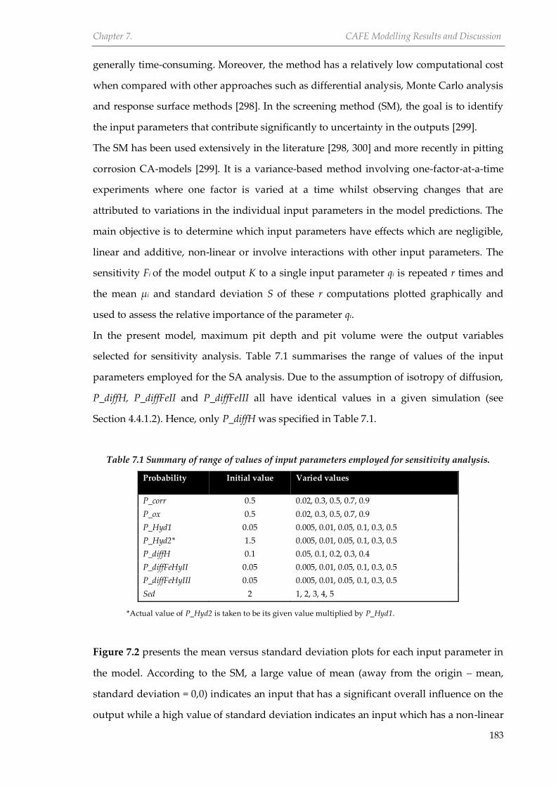
Chapter 7. CAFE Modelling Results and Discussion
183
generally time-consuming. Moreover, the method has a relatively low computational cost
when compared with other approaches such as differential analysis, Monte Carlo analysis
and response surface methods [298]. In the screening method (SM), the goal is to identify
the input parameters that contribute significantly to uncertainty in the outputs [299].
The SM has been used extensively in the literature [298, 300] and more recently in pitting
corrosion CA-models [299]. It is a variance-based method involving one-factor-at-a-time
experiments where one factor is varied at a time whilst observing changes that are
attributed to variations in the individual input parameters in the model predictions. The
main objective is to determine which input parameters have effects which are negligible,
linear and additive, non-linear or involve interactions with other input parameters. The
sensitivity Fi of the model output K to a single input parameter qi is repeated r times and
the mean µi and standard deviation S of these r computations plotted graphically and
used to assess the relative importance of the parameter qi.
In the present model, maximum pit depth and pit volume were the output variables
selected for sensitivity analysis. Table 7.1 summarises the range of values of the input
parameters employed for the SA analysis. Due to the assumption of isotropy of diffusion,
P_diffH, P_diffFeII and P_diffFeIII all have identical values in a given simulation (see
Section 4.4.1.2). Hence, only P_diffH was specified in Table 7.1.
Table 7.1 Summary of range of values of input parameters employed for sensitivity analysis.
Probability Initial value Varied values
P_corr 0.5 0.02, 0.3, 0.5, 0.7, 0.9
P_ox 0.5 0.02, 0.3, 0.5, 0.7, 0.9
P_Hyd1 0.05 0.005, 0.01, 0.05, 0.1, 0.3, 0.5
P_Hyd2* 1.5 0.005, 0.01, 0.05, 0.1, 0.3, 0.5
P_diffH 0.1 0.05, 0.1, 0.2, 0.3, 0.4
P_diffFeHyII 0.05 0.005, 0.01, 0.05, 0.1, 0.3, 0.5
P_diffFeHyIII 0.05 0.005, 0.01, 0.05, 0.1, 0.3, 0.5
Sed 2 1, 2, 3, 4, 5
*Actual value of P_Hyd2 is taken to be its given value multiplied by P_Hyd1.
Figure 7.2 presents the mean versus standard deviation plots for each input parameter in
the model. According to the SM, a large value of mean (away from the origin – mean,
standard deviation = 0,0) indicates an input that has a significant overall influence on the
output while a high value of standard deviation indicates an input which has a non-linear

Chapter 7. CAFE Modelling Results and Discussion
184
influence on the output or an input whose effect on the output depends on its interaction
with other input parameters [298, 300]. The relative importance of each of the input
parameters can also be measured by defining a sensitivity measure: the Euclidean
distance from the origin in the (µ, S) space, denoted by δ. The plots for maximum pit
depth and pit volume, which are presented in Figures 7.2a and 7.2b, generally show the
same trend due to the direct relationship between both outputs. The values of mean for all
the parameters are substantially different from zero, indicating that the pit depth and pit
volume are sensitive to all the input parameters of the model. Similarly, the standard
deviation for each of the input parameters are large, indicating that they have non-linear
effects which depend on their interaction with other input parameters (relatively large S
values). The order of importance 𝛿 determined for all the input factors is summarised in
Table 7.2 and Table 7.3 for maximum pit depth and pit volume respectively. Comparison
of the values shows that all the input parameters are equally important for determining
localised corrosion behaviour. The exceptions are the probabilities of diffusion of acidic
sites (P_diffH) and iron II ions (P_diffFeHyII) and iron III ions (P_diffFeHyII), which are the
most important.
mean (m)
120 140 160 180 200 220 240
Sta
ndard
devia
tion
0
25
50
75
100
125
150
P_corr
P_ox
P_Hyd1
P_Hyd2
P_diffFeHyII
P_diffFeHyIII
Sed
P_diffH
(a)

Chapter 7. CAFE Modelling Results and Discussion
185
meanx 108 (cm
3)
15 20 25 30 35 40
Sta
ndard
devia
tion
0
5
10
15
20
25
30
P_corr
P_ox
P_Hyd1
P_Hyd2
P_diffFeHyII
P_diffFeHyIII
Sed
P_diffH
Figure 7.2 µ-S plots for each of the input parameters associated with (a) maximum pit depth and
(b) pit volume.
Table 7.2 Summary of values of the three sensitivity measures µ, S and 𝜹 associated with the
maximum pit depth for each of the input parameters.
Probability µ (µm) S (µm) 𝜹
P_corr 203 24 204
P_ox 204 22 205
P_Hyd1 198 55 206
P_Hyd2 205 51 211
P_diffH 223 138 263
P_diffFeHyII 187 34 190
P_diffFeHyIII 133 107 171
Sed 161 114 198
Table 7.3 The values of the three sensitivity measures µ, S and 𝜹 associated with the pit volume for
each of the input parameters.
Probability µ x 107 (cm3) S x 107 (cm3) 𝜹 x 107
P_corr 3.23 0.62 3.36
P_ox 3.24 0.90 3.24
P_Hyd1 3.12 1.18 3.34
P_Hyd2 3.34 1.10 3.52
P_diffH 3.34 2.64 4.25
P_diffFeHyII 2.90 6.36 2.97
P_diffFeHyIII 1.96 1.87 2.71
Sed 2.56 2.18 3.36
(b)

Chapter 7. CAFE Modelling Results and Discussion
186
These SA results underscore the complex interactions occurring between several
competing and complex processes taking place during localized corrosion. For instance,
increasing the probability of oxidation of Fe to Fe2+ (P_corr) and probability of oxidation of
Fe2+ to Fe3+ (P_ox) will potentially increase the initial rate of metal dissolution. However,
this effect depends on the availability of acidic sites, which depends on the probability of
its diffusion (P_diffH) and rate of accumulation of corrosion products that are formed as
corrosion progresses. Hydrolysis is a process that can increase or decrease the rate of
corrosion but these effects depend on the availability of water sites and species that are
formed as a result of the oxidation process. Accumulation of corrosion products can
decrease corrosion rate by creating a diffusion barrier for corrosion species but this also
depends on the rate of precipitation of corrosion products (Sed), which in turn is related to
the probability for hydrolysis (P_Hyd1/P_Hyd2).
7.4 Influence of model parameters
Localised corrosion is a complex stochastic process whose kinetics can be affected by
several mechanisms including metal dissolution, diffusion, precipitation, and hydrolysis,
all of which have non-linear behaviour. In the present system, different parameters were
defined that account for these processes and their stochastic nature. From the sensitivity
analysis carried in the previous section, all the input parameters were found to influence
the model outputs. Moreover, they also show interactions with each other. The behaviour
of the CA model was investigated further by evaluating the roles of selected input
parameters on the time-dependent localised corrosion kinetics and evolution of pit depth
and pit volume. Due to computational time limitations, the parameters selected for
further investigation include; oxidation of metal to Fe2+ denoted by P_corr, oxidation of
Fe2+ to Fe3+ denoted by P_ox, hydrolysis of Fe2+ to Fe(OH)2 denoted by P_Hyd1 and
precipitation of Fe(OH)2 and Fe(OH)3 denoted by Sed.
Simulations were carried out by varying the values of each of these probabilities and
fixing other input parameters. The resulting pit depth and pit volume versus time profiles
were determined from the simulations, which were undertaken using a 1000 x 500 lattice.
The width of each cell in the lattice was set to 2.5 µm. Theoretical and experimental data
are also shown on the profiles for the purpose of comparison. Theoretical pit depths were
obtained from Faraday’s law (see Section 3.8.2). The following probabilities were

Chapter 7. CAFE Modelling Results and Discussion
187
employed for the input parameters for the simulations: P_corr – 0.2, P_ox – 0.2, Phyd1 –
0.09, P_Hyd2 – 1.5 P_Hyd1, P_DiffH – 0.5, P_DiffFeII – 0.5, P_DiffFeIII – 0.5, P_DifFeHydII –
0.06, P_DifFeHydIII – 0.06, Sed – 3.4.
7.4.1 Effect of oxidation of Fe to Fe2+
The probability of corrosion, P_corr, was introduced in the model to simulate the rate at
which Fe is oxidized to Fe2+. Higher probability for corrosion increases the tendency for
oxidation, increases the concentration of the corrosion specie, Fe2+, and consequently the
rate of metal dissolution. Figure 7.3 shows the variation of maximum pit depth and pit
volume with time at various P_corr values. The same trend is generally observed for both
pit volume and maximum pit depth i.e. power law relationship with time. This is
expected because of the correlation between metal loss (pit volume) and pit depth as
described by Faraday’s law [301]. It has been observed that a power-law relationship
generally exists between both maximum pit depth and pit volume and time [124, 302].
These results illustrate the time-dependent nature of localised corrosion damage and the
characteristic role of diffusion in this process. These results illustrate the time-dependent
nature of localised corrosion damage and the characteristic role of diffusion in this
process.
(a)

Chapter 7. CAFE Modelling Results and Discussion
188
Figure 7.3. The role of different corrosion probabilities on time-dependent localised corrosion
behaviour. (a) maximum pit depth and (b) pit volume.
The amount of damage generally increases with increase in probability but was not
significantly different at P_corr values of 0.2 and 0.3. This is thought to be a consequence
of diffusion processes whereby there will be a limit to which increasing the rate of
oxidation (increasing P_corr) will have a substantial effect on dissolution rate. The rate of
localised damage will be controlled by the diffusion processes simulated with diffusion
probabilities in the model rather than oxidation rate of Fe to Fe2+.
7.4.2 Effect of accumulation of corrosion products
As mentioned earlier, a sedimentation factor, Sed, was introduced into the model to
account for accumulation of corrosion products (Fe(OH)2 and Fe(OH)3) during localised
dissolution. This simulates a stagnant system where the corrosion products are not able to
be conveyed away from the pit through mass transport, which would otherwise be
possible in a flowing system. The variation of maximum pit depth and pit volume with
time at various Sed values is shown in Figure 7.4. It can be observed that higher values of
Sed result in lower values of maximum pit depth and pit volume at a given time interval.
In addition, for a given Sed value, the rate of damage decreases with time. This generally
indicates that an increase in the rate of accumulation of corrosion products (increase in
Sed) redcues the rate of damage by reducing pit growth and metal loss rate. This
accumulation can determine the rate of metal dissolution through a diffusion control
(b)
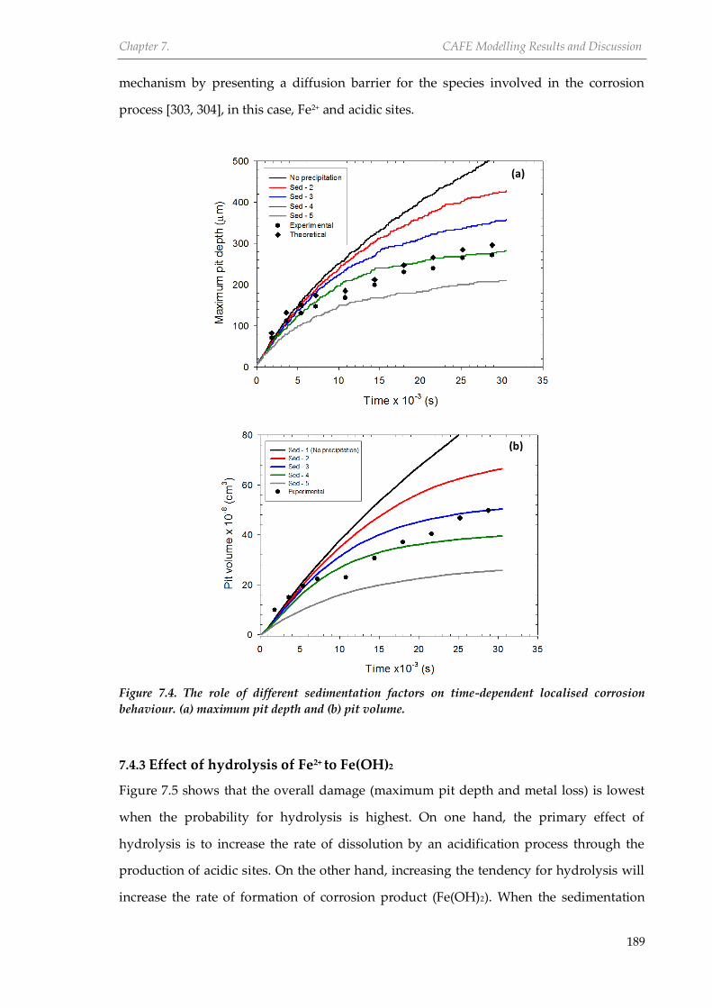
Chapter 7. CAFE Modelling Results and Discussion
189
mechanism by presenting a diffusion barrier for the species involved in the corrosion
process [303, 304], in this case, Fe2+ and acidic sites.
Figure 7.4. The role of different sedimentation factors on time-dependent localised corrosion
behaviour. (a) maximum pit depth and (b) pit volume.
7.4.3 Effect of hydrolysis of Fe2+ to Fe(OH)2
Figure 7.5 shows that the overall damage (maximum pit depth and metal loss) is lowest
when the probability for hydrolysis is highest. On one hand, the primary effect of
hydrolysis is to increase the rate of dissolution by an acidification process through the
production of acidic sites. On the other hand, increasing the tendency for hydrolysis will
increase the rate of formation of corrosion product (Fe(OH)2). When the sedimentation
(a)
(b)

Chapter 7. CAFE Modelling Results and Discussion
190
factor is large enough, more corrosion products accumulate and consequently result in
less damage as discussed above (Section 7.4.2).
Figure 7.6. The influence of different hydrolysis probabilities on time-dependent localised
corrosion behaviour. (a) maximum pit depth and (b) pit volume.
7.5 Model validation
The usefulness of the CAFE model lies in its ability to predict the time-dependent
evolution of depth and geometry of pits and their associated strain distribution. To ensure
that the model can simulate this time-dependent behaviour, its outputs can be compared
with available experimental data through a validation process. As discussed in Sections
7.3 and 7.4, the values of the input parameters determined the time-dependent evolution
of pit depth and pit geometry. Therefore, the validity of the model will depend on a
combination of specific values for each of the defined input probabilities. Since the model
(a)
(b)

Chapter 7. CAFE Modelling Results and Discussion
191
possesses several input parameters, optimization was necessary to obtain a combination
of a specific set of values for each of the input parameters. The optimized model was
obtained by evaluating different combinations of values of input parameters that
minimises the disparity between model predictions and experimental data. The model
was optimized to simulate the two sets of experiments that were carried out in the present
work i.e. with and without (stagnant) flow. The values of probabilities obtained for the
optimized models in each case are given in Table 7.4.
Table 7.4 Summary of probabilities obtained for optimized models for stagnant (without flow)
and flow conditions.
Probability Stagnant With flow
P_corr 0.19 0.20
P_ox 0.30 0.30
P_Hyd1 0.15 0.15
P_Hyd2 0.30 0.30
P_diffH 0.50 0.50
P_diffFeHyII 0.06 0.06
P_diffFeHyIII 0.06 0.06
Sed 3.30 1.10
Representative results obtained from the optimized models together with the
experimental data for stagnant and flowing conditions are shown in Figure 7.6 and Figure
7.7 respectively.
Time x 10-3
(s)
0 5 10 15 20 25 30 35
Maxim
um
pit d
epth
(
m)
0
100
200
300
Theoretical model
Experimental
CA Model
(a)

Chapter 7. CAFE Modelling Results and Discussion
192
Time x 10-3
(s)
0 5 10 15 20 25 30 35
Aspect ra
tio
0.2
0.4
0.6
0.8
Experimental
CA Model
Figure 7.6 Plots of (a) maximum pit depth and (b) pit aspect ratio as a function of time simulating
pit growth under stagnant (without flow) conditions.
Figures 7.6a and 7.7a show that the model predictions for maximum pit depth show good
agreement with experimental data. In terms of pit aspect ratio, correlation with
experimental data was better under stagnant conditions than under flow conditions.
Although these results are satisfactory, further model refinement is still needed to
minimize the variance between the model predictions and experiment results. The results
from three simulations for each model are summarised in Appendix C.
Time x 10-3
(s)
0 20 40 60 80 100
Maxim
um
pit d
epth
(
m)
0
200
400
600
800
Experimental
CA Model
(b)
(a)

Chapter 7. CAFE Modelling Results and Discussion
193
Time x 10-3
(s)
0 20 40 60 80 100
Aspect ra
tio
0.0
0.4
0.8
1.2
1.6
2.0
Experimental
CA Model
Figure 7.7 Plot of (a) maximum pit depth and (b) pit aspect ratio as a function of time simulating
pit growth under flow conditions.
Comparison between the input parameters for the two models (see Table 7.4) shows that
the only difference is the sedimentation factor, which accounts for the accumulation of
corrosion products (Fe(OH)2 and Fe(OH)3). Compared to a Sed value of 3.3 for static
conditions, a lower value of 1.1 under flowing conditions indicates a relatively lower
tendency for corrosion products to accumulate due the mass transport effect of flow [304].
Consequently, the resulting diffusion barrier to corrosion species will be minimized, the
rate of metal loss will increase [304] and rate of pit growth will be higher compared to
when there is no flow [265].
Figure 7.8 shows the cross-sectional profiles of the pits obtained from the CA model at
different times under stagnant conditions compared to the corresponding cross-sectional
profiles of those obtained experimentally. It can be seen that both sets of data show good
correlation, in terms of pit depth and pit width. The disparity between both sets of data in
Figure 7.6 is not apparent in the cross-sectional profiles. This is because the plots shown in
Figure 7.6a are for maximum pit depth, which is defined in the model as the numerical
difference between the minimum and maximum points in the metal space rather than
average pit depth (plotted for experimental data). The same is applicable to the plots for
the pit width (Figure 7.6b). It can also be observed from Figure 7.8 that the profiles
obtained from the model are not as smooth as those from the experiments. This is due to
(b)

Chapter 7. CAFE Modelling Results and Discussion
194
the size of the lattice employed for the study (1000 x 500) for which the cell size is 2.5 µm.
Increasing the size of the lattice will smoothen the pit profile but will increase
computation time exponentially.
Distance (m)
200 400 600 800 1000 1200
Pit d
epth
(
m)
-500
-400
-300
-200
-100
0
Experiment
CA Model
Distance (m)
200 400 600 800 1000 1200
Pit d
epth
(
m)
-500
-400
-300
-200
-100
0
Experiment
CA Model
Distance (m)
200 400 600 800 1000 1200
Pit d
epth
(
m)
-500
-400
-300
-200
-100
0
Experiment
CA Model
Distance (m)
200 400 600 800 1000 1200
Pit d
epth
(
m)
-500
-400
-300
-200
-100
0
Experiment
CA Model
Distance (m)
200 400 600 800 1000 1200
Pit d
epth
(
m)
-500
-400
-300
-200
-100
0
Experiment
CA Model
Distance (m)
200 400 600 800 1000 1200
Pit d
epth
(
m)
-500
-400
-300
-200
-100
0
Experiment
CA Model
Figure 7.8 Comparison between cross-sectional profiles of pits obtained from experiment and CA
model at different times.
The results show good agreement between experimental data and the outputs of the
model (maximum depth, width and cross-sectional profiles of the pits). This gives
Time = 1800 s Time = 3600 s
Time = 7200 s Time = 14400 s
Time = 18000 s Time = 25200 s
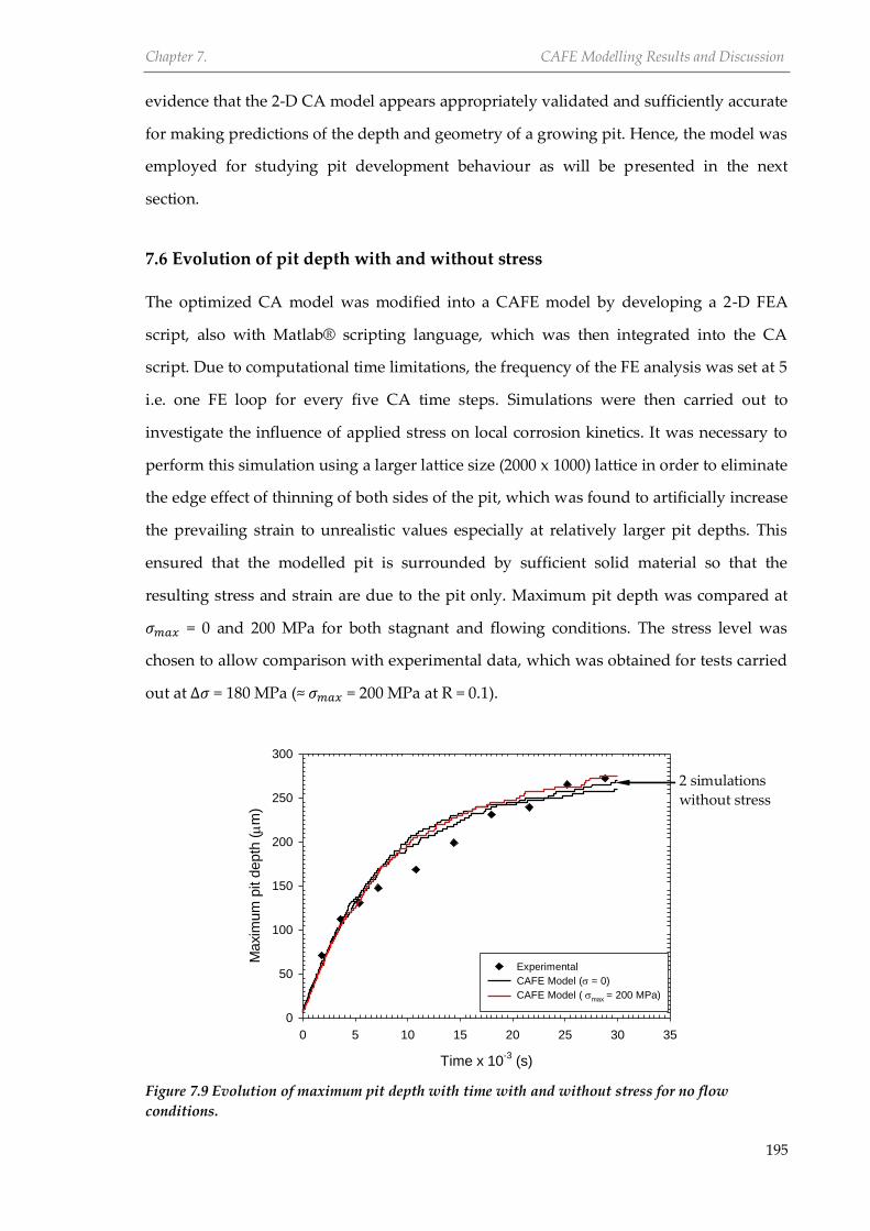
Chapter 7. CAFE Modelling Results and Discussion
195
evidence that the 2-D CA model appears appropriately validated and sufficiently accurate
for making predictions of the depth and geometry of a growing pit. Hence, the model was
employed for studying pit development behaviour as will be presented in the next
section.
7.6 Evolution of pit depth with and without stress
The optimized CA model was modified into a CAFE model by developing a 2-D FEA
script, also with Matlab® scripting language, which was then integrated into the CA
script. Due to computational time limitations, the frequency of the FE analysis was set at 5
i.e. one FE loop for every five CA time steps. Simulations were then carried out to
investigate the influence of applied stress on local corrosion kinetics. It was necessary to
perform this simulation using a larger lattice size (2000 x 1000) lattice in order to eliminate
the edge effect of thinning of both sides of the pit, which was found to artificially increase
the prevailing strain to unrealistic values especially at relatively larger pit depths. This
ensured that the modelled pit is surrounded by sufficient solid material so that the
resulting stress and strain are due to the pit only. Maximum pit depth was compared at
𝜎𝑚𝑎𝑥 = 0 and 200 MPa for both stagnant and flowing conditions. The stress level was
chosen to allow comparison with experimental data, which was obtained for tests carried
out at ∆𝜎 = 180 MPa (≈ 𝜎𝑚𝑎𝑥 = 200 MPa at R = 0.1).
Time x 10-3
(s)
0 5 10 15 20 25 30 35
Maxim
um
pit d
epth
(
m)
0
50
100
150
200
250
300
Experimental
CAFE Model (= 0)
CAFE Model (max= 200 MPa)
Figure 7.9 Evolution of maximum pit depth with time with and without stress for no flow
conditions.
2 simulations
without stress
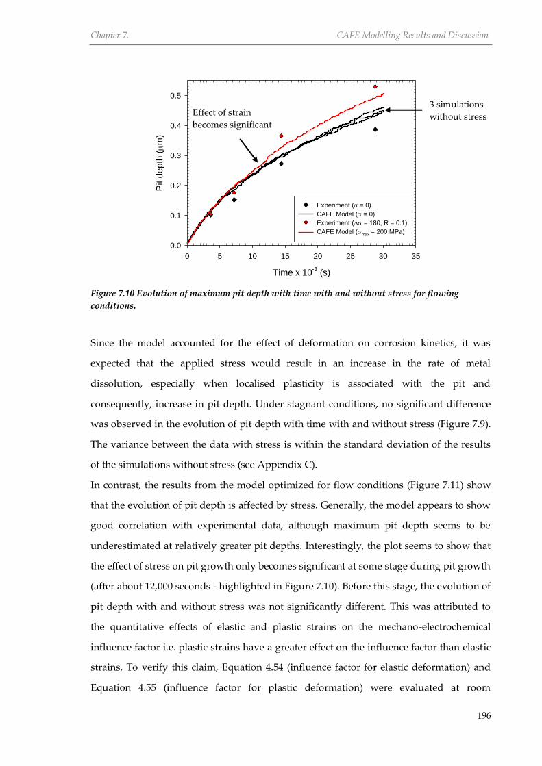
Chapter 7. CAFE Modelling Results and Discussion
196
Time x 10-3
(s)
0 5 10 15 20 25 30 35
Pit d
epth
(
m)
0.0
0.1
0.2
0.3
0.4
0.5
Experiment ( = 0)
CAFE Model ( = 0)
Experiment ( = 180, R = 0.1)
CAFE Model (max= 200 MPa)
Figure 7.10 Evolution of maximum pit depth with time with and without stress for flowing
conditions.
Since the model accounted for the effect of deformation on corrosion kinetics, it was
expected that the applied stress would result in an increase in the rate of metal
dissolution, especially when localised plasticity is associated with the pit and
consequently, increase in pit depth. Under stagnant conditions, no significant difference
was observed in the evolution of pit depth with time with and without stress (Figure 7.9).
The variance between the data with stress is within the standard deviation of the results
of the simulations without stress (see Appendix C).
In contrast, the results from the model optimized for flow conditions (Figure 7.11) show
that the evolution of pit depth is affected by stress. Generally, the model appears to show
good correlation with experimental data, although maximum pit depth seems to be
underestimated at relatively greater pit depths. Interestingly, the plot seems to show that
the effect of stress on pit growth only becomes significant at some stage during pit growth
(after about 12,000 seconds - highlighted in Figure 7.10). Before this stage, the evolution of
pit depth with and without stress was not significantly different. This was attributed to
the quantitative effects of elastic and plastic strains on the mechano-electrochemical
influence factor i.e. plastic strains have a greater effect on the influence factor than elastic
strains. To verify this claim, Equation 4.54 (influence factor for elastic deformation) and
Equation 4.55 (influence factor for plastic deformation) were evaluated at room
3 simulations
without stress Effect of strain
becomes significant

Chapter 7. CAFE Modelling Results and Discussion
197
temperature (298 0K) using elastic and plastic strains obtained from finite element analysis
of an idealised 3-D pit model. Numerical values of the elastic strain at a point just before
onset of plasticity and plastic strain after yielding (equivalent plastic strain - PEEQ of
0.1%) were applied as inputs to the equations. The influence factor obtained was 1.03 for
elastic strain compared to 1.33 for the plastic strain. Conceptually, this means that a given
P_corr value will increase by a factor of 1.03 and 1.33 for elastic and plastic deformation
respectively. Hence, a higher probability for oxidation of Fe to Fe2+ when there is localised
plasticity compared to when there is none. Also in Figure 7.10, similar to the experimental
results, the difference between the maximum pit depth-time plots with and without stress
seems to be increasing progressively with time as the pit become deeper. This agrees with
earlier discussion of the effect of stress on corrosion rate. The onset of plasticity increases
the probability for oxidation of metal, which may result in development of deeper pits. At
a given applied stress level, the plasticity associated with a growing pit (increasing size)
will likely increase progressively with pit size, thereby increasing the pit growth rate.
Comparison between the results presented in Figures 7.9 and 7.10 shows that, whereas the
local corrosion kinetics was not affected significantly by applied stress under stagnant
conditions, the influence was apparent under flow conditions. This suggests that the
influence of mechanical stress depends on other processes taking place in the pit, in this
case, accumulation of corrosion products. Although, deformation (through the mechano-
electrochemical effect) may increase the tendency for dissolution [252, 305] i.e. oxidation
of the Fe (metal sites) to Fe2+, the accumulated corrosion products presented a diffusion
barrier to the reaction species (in this case the acidic sites) required for oxidation to
proceed. Consequently, the rate of metal loss remains unchanged as when no stress is
applied. In the model simulating flow, the reduction in the rate of accumulation of
corrosion products (i.e. relatively lower Sed value of 1.1) results in a lower diffusion
barrier. This coupled with the increased tendency for oxidation as a result of deformation,
will effectively increase the rates of anodic dissolution and pit growth.
7.7 Evolution of stress and strain with time
Understanding the evolution and distribution of stress and strain associated with time-
dependent changes in geometry of a growing pit, in a stressed component, is important in
order predict the conditions necessary for the transition of a pit to crack. Apart from the

Chapter 7. CAFE Modelling Results and Discussion
198
mechano-electrochemical effect on corrosion kinetics, applied stress also induces local
dynamic strain, which is recognized to result in nucleation of cracks around a pit [202].
When plasticity is significant, accumulation of plastic strains and changes in plastic strain
rates increases the dynamic strains and consequently the susceptibility to cracking. Given
that the simulation of continuous growth of a corrosion pit in 3-D is difficult, previous
attempts to evaluate the distribution of stress and strain around pits have been based on a
discretized approach whereby pit sizes at different stages during pit development are
idealized as elliptical/hemispherical models on which FEA is conducted [1, 201, 230, 248,
306, 307]. More recently, the discretized approach has been improved to account for
accumulated plasticity by simulating increment in pit size (pit growth) in a step-wise
manner with retention of the history of the previous step [202]. Although this approach
showed more accurate results, the number of pit size increments that can be simulated is
limited. Furthermore, some assumptions regarding pit shape and actual pit depth have to
be made. From a mechanics-based point of view, the CAFE model can help to overcome
these challenges because:
1. No assumptions are required concerning changes depth, aspect ratio, morphology
and shape symmetry of a growing pit (with time). Strains associated with actual
pits simulated by the model are evaluated.
2. The influence of elastic and plastic deformation on corrosion kinetics and strain
localization is accounted for.
3. Strain distribution corresponding to each pit size at every time step and its
evolution during pit growth can all be evaluated automatically.
Typical Von Mises stress and total strain (maximum principal strain) distributions around
the 2-D pits obtained at different time intervals in a direction parallel to loading are
shown in Figure 7.11 and Figure 7.12 respectively. The results generally show that the
distribution and evolution of stress and strain around a growing pit can be monitored and
evaluated at every stage during pit development irrespective of depth, aspect ratio and
morphology of the pit using the CAFE model. Whereas the extent of strain localization
(evaluated as maximum principal strain) generally increased with time, pit depth and pit
aspect ratio, the maximum effective stress did not change significantly for the range of pit
depths shown. The latter indicates localised yielding given the yield strength of 530 MPa
for this material.

Chapter 7. CAFE Modelling Results and Discussion
199
Figure 7.11 Evolution and distribution of equivalent stress around a growing pit in a static stress
field simulated with the 2-D CAFE model. (𝝈𝒎𝒂𝒙 = 200 MPa).
Time = 3600 seconds
Max. pit depth = 101 µm
Aspect ratio = 0.38
Time = 18000 seconds
Max. pit depth = 242 µm
Aspect ratio = 0.73
Time = 7200 seconds
Max. pit depth = 162 µm
Aspect ratio = 0.55
Time = 10800 seconds
Max. pit depth = 195 µm
Aspect ratio = 0.64

Chapter 7. CAFE Modelling Results and Discussion
200
Figure 7.12 Evolution and distribution of total strain around a growing pit in a static stress field
simulated with the 2-D CAFE model. (𝝈𝒎𝒂𝒙 = 200 MPa).
Time = 3600 seconds
Max. pit depth = 101 µm
Aspect ratio = 0.38
Time = 10800 seconds
Max. pit depth = 195 µm
Aspect ratio = 0.64
Time = 7200 seconds
Max. pit depth = 162 µm
Aspect ratio = 0.55
Time = 18000 seconds
Max. pit depth = 242 µm
Aspect ratio = 0.73
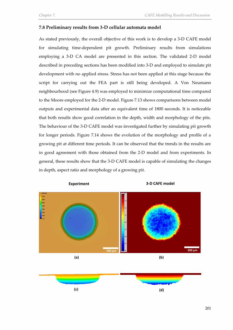
Chapter 7. CAFE Modelling Results and Discussion
201
7.8 Preliminary results from 3-D cellular automata model
As stated previously, the overall objective of this work is to develop a 3-D CAFE model
for simulating time-dependent pit growth. Preliminary results from simulations
employing a 3-D CA model are presented in this section. The validated 2-D model
described in preceding sections has been modified into 3-D and employed to simulate pit
development with no applied stress. Stress has not been applied at this stage because the
script for carrying out the FEA part is still being developed. A Von Neumann
neighbourhood (see Figure 4.9) was employed to minimize computational time compared
to the Moore employed for the 2-D model. Figure 7.13 shows comparisons between model
outputs and experimental data after an equivalent time of 1800 seconds. It is noticeable
that both results show good correlation in the depth, width and morphology of the pits.
The behaviour of the 3-D CAFE model was investigated further by simulating pit growth
for longer periods. Figure 7.14 shows the evolution of the morphology and profile of a
growing pit at different time periods. It can be observed that the trends in the results are
in good agreement with those obtained from the 2-D model and from experiments. In
general, these results show that the 3-D CAFE model is capable of simulating the changes
in depth, aspect ratio and morphology of a growing pit.
(a) (b)
(c) (d)
3-D CAFE model Experiment
200 µm 200 µm
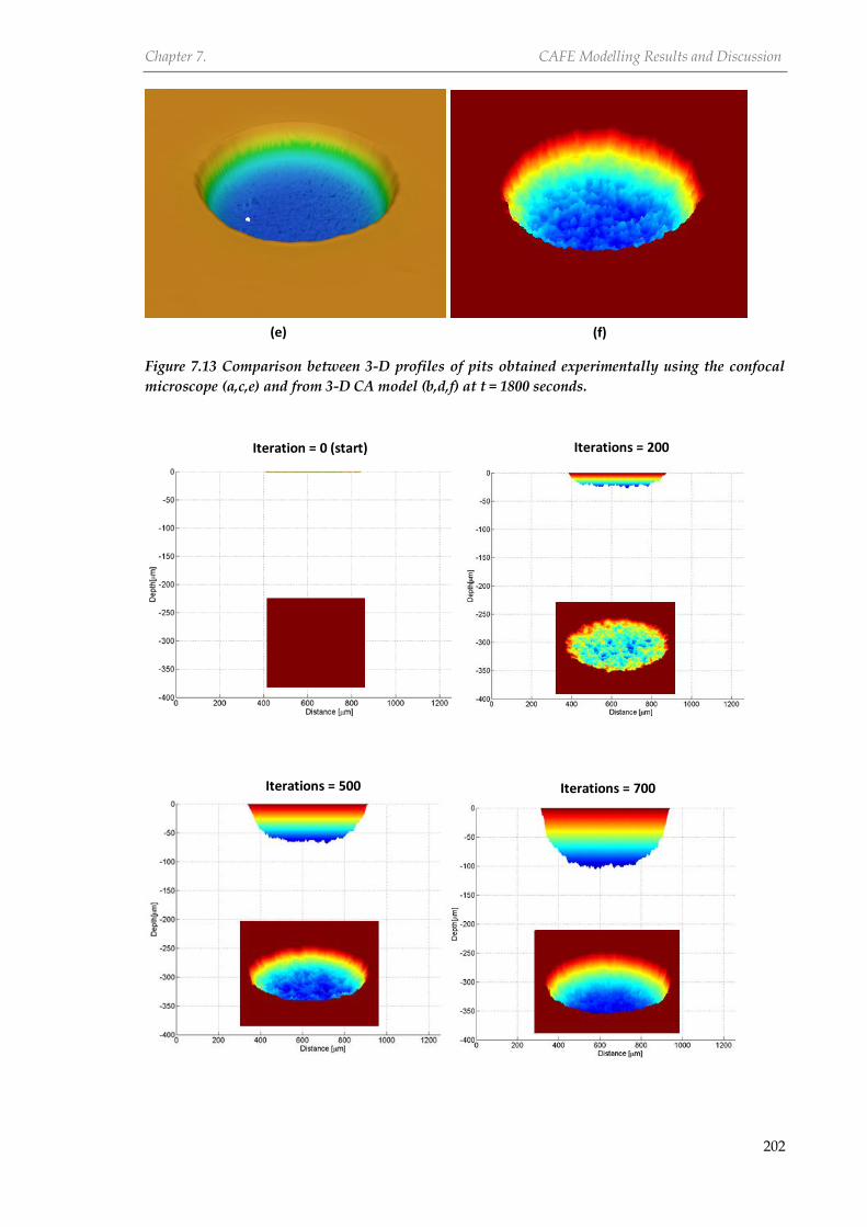
Chapter 7. CAFE Modelling Results and Discussion
202
Figure 7.13 Comparison between 3-D profiles of pits obtained experimentally using the confocal
microscope (a,c,e) and from 3-D CA model (b,d,f) at t = 1800 seconds.
(f) (e)
Iteration = 0 (start) Iterations = 200
Iterations = 500 Iterations = 700
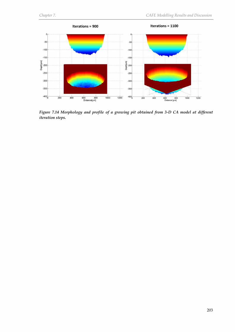
Chapter 7. CAFE Modelling Results and Discussion
203
Figure 7.14 Morphology and profile of a growing pit obtained from 3-D CA model at different
iteration steps.
Iterations = 1100 Iterations = 900

Chapter 8
Fatigue Lifetime
Modelling

Chapter 8. Fatigue Lifetime Modelling
205
8.1 Introduction
Corrosion fatigue is a damage process occurring due to synergistic interaction of
electrochemical, metallurgical and mechanical loading. A predictive approach to lifetime
management based on quantifying the evolution of damage from the earliest stage,
including crack precursor development, is a major undertaking that requires
developments in mechanistic understanding of the controlling processes and modelling
capability. In this chapter, an attempt has been made to develop suitable multi-stage
lifetime models for the air and corrosion fatigue tests carried out in the present study.
8.2 Multi-stage damage accumulation model
The core feature of the present predictive scheme is the quantification of the rate of
damage development during the corrosion fatigue process; a damage process divided into
the following four stages:
1. Pit development
2. Pit-to-crack transition
3. Short crack growth and
4. Long crack growth
Individual empirical model(s) have been developed for predicting the lifetimes (number
of cycles) spent in each these regimes as a function of pit size, microstructure,
environment and stress. The total fatigue lifetime is the accumulated lifetimes expressed
as
𝑁𝑇𝑜𝑡𝑎𝑙 = 𝑁𝑝𝑔 + 𝑁𝑝𝑡𝑐 + 𝑁𝑠𝑐 + 𝑁𝑙𝑐 8.1
where 𝑁𝑇𝑜𝑡𝑎𝑙 is total fatigue life, 𝑁𝑝𝑔 is lifetime taken to generate a pit to specified depth,
𝑁𝑝𝑡𝑐 is lifetime to nucleate a crack from a pit, 𝑁𝑠𝑐 is lifetime to propagate a crack up to the
dominant microstructural barrier, and 𝑁𝑙𝑐is lifetime taken to propagate the crack beyond
this barrier until failure of the specimen. It is worth emphasizing the entire model
development effort is based on corrosion fatigue systems where corrosion pits are
precursors to fatigue cracks. Hence, material-environment systems where cracks emanate
from defects other than corrosion pits are not considered. It was assumed that scale/film
breakdown has already taken place so that active anodic dissolution of the underlying

Chapter 8. Fatigue Lifetime Modelling
206
metal through pit development is the first stage. In subsequent sections, the models
developed for each of the different stages are presented.
8.2.1 Modelling pit growth
The time-dependent pit growth stage involves the evolution of damage (pit depth) with
time. The relationship between pit depth and time may be expressed in the form
𝑑𝑝 = 𝐴𝑝𝑔 ∙ 𝑡𝑛𝑝𝑔 8.2
where 𝑑𝑝 is maximum pit depth (µm), 𝑡 is time (hours), and 𝐴𝑝𝑔 and 𝑛𝑝𝑔 are the pit
growth coefficient and exponent respectively both of which depend on the metal-
environment system. These constants were determined by fitting Equation 8.1 to the
maximum pit depth-time experimental data obtained for tests conducted with and
without stress. The values obtained for 𝐴𝑝𝑔 and 𝑛𝑝𝑔 are 104.2 and 0.654 for the unstressed
test (Δσ = 0) and 118.5 and 0.640 at Δσ = 180 MPa respectively. The coefficient, 𝐴𝑝𝑔, show a
dependency on stress hence, it was expressed as a function of stress range (Equation 8.2)
in order to capture the effect of stress on pit growth.
𝐴𝑝𝑔 = 104.242 (1.008) ∆𝜎 8.3
where ∆𝜎 is the applied stress range (MPa).
Therefore, the general equation for predicting pit development as a function of time was
expressed as
𝑑𝑝 = 104.2 (1.008) ∆𝜎 ∙ 𝑡0.645 8.4
The pit depths predicted from this model at a given stress range (Figure 8.1) show good
correlation with experimental data.
From Equation 8.3, the pit growth lifetime, 𝑁𝑝𝑔, i.e. number of cycles required to generate
a pit of given depth can be predicted by expressing 𝑡 as a function of cyclic frequency, 𝑓,
(i.e. 𝑁 = 𝑡 ∙ 𝑓) as given below.
𝑁𝑝𝑔 = 3600 ∙ 𝑓 [
𝑑𝑝
104.242 (1.0076) ∆𝜎]
1
0.645
8.5

Chapter 8. Fatigue Lifetime Modelling
207
Experimental pit depth (m)
100 1000
Pre
dic
ted p
it d
epth
(
m)
100
1000 Unstressed
Stressed (= 180 MPa)
Figure 8.1 Comparison between experimental and predicted pit depths from pit growth model.
It is recognized that the constants in Equation 8.4 are based on experimental data from
only two stress levels. For the model to be applicable at other stress levels, new values of
constants should be evaluated from the experimental data for stress ranges of interest.
Nevertheless, for analysis purposes, the constants were assumed to be valid at all stress
ranges. Based on Equation 8.4, pit growth lifetime calculations were made for a given pit
depth, stress range and test frequency (2 Hz for the present study).
8.2.2 Modelling pit-to-crack transition lifetimes
The number of cycles to crack initiation in air and corrosion fatigue were experimentally
observed to depend on applied stress and pit size. It is therefore important to predict pit-
to-crack transition lifetimes as a function of these two variables. The relationship between
crack initiation lifetime for single pits, 𝑁𝑝𝑡𝑐, and pit aspect ratio, 𝐴𝑅𝑝, can be expressed as
𝑁𝑝𝑡𝑐 = 𝐺 ∙ (𝐴𝑅𝑝)𝑔 8.6
where G and 𝑔 are material-environment constants. The values of G and 𝑔 in air and
corrosion fatigue, given in Table 8.1, were determined by regression analysis of 𝑁𝑝𝑡𝑐 −
𝐴𝑅𝑝 experimental data obtained at different stress ranges. Both constants depend on stress
hence, both were expressed as a function of stress range, ∆𝜎, as given in Equations 8.7 and
8.8.
±10% error band

Chapter 8. Fatigue Lifetime Modelling
208
𝐺 = 𝐾 ∙ (∆𝜎 )𝑝 8.7
𝑔 = 𝐿 ∙ (∆𝜎 )𝑞 8.8
The values obtained for the constants by regression analysis of data in Table 8.1 are:
K = 1.6 x 1043, L = -1.2 x 10¹³, p = -14.088, and q = -4.811 (air)
K = 8.0 x 10²⁰, L = -1.3 x 10⁵, p = -5.974, and q = -1.845 (corrosion fatigue)
Table 8.1 Summary of material constants for pit-to-crack transition lifetime equation.
Air fatigue Corrosion fatigue
Δσ (MPa) 𝑮 𝒈 𝑮 𝒈
405 2.423 x 10⁶ -3.676 2.056 x 10⁵ -1.983
427.5 2.046 x 10⁶ -2.342 1.623 x 10⁵ -1.752
450 5.434 x 10⁵ -2.222 1.094 x 10⁵ -1.634
Substituting Equations 8.7 and 8.8 into Equation 8.6 yields Equation 8.9, which predicts
pit-to-crack transition lifetimes for known stress range and pit aspect ratio. This model is
based on the assumption that the stress range-pit depth combination has satisfied the pit-
to-crack transition conditions in air and corrosion fatigue i.e. either the stress range is
above the fatigue limit associated with a particular pit size or the pit depth is above the
critical size that will initiate a crack.
𝑁𝑝𝑡𝑐 = 𝐾 ∙ (∆𝜎)𝑝 ∙ (𝐴𝑅𝑝)𝐿∙(∆𝜎)𝑞 8.9
Based on Equation 8.9, pit-to-crack transition lifetimes were calculated for air and
corrosion fatigue environments. The predicted lifetimes together with experimental data
are shown in Figure 8.2.

Chapter 8. Fatigue Lifetime Modelling
209
Experimental Nptc (cycles)
105 106 107
Pre
dic
ted N
ptc
(cyc
les)
105
106
107
= 427.5 MPa, dp = 140 m
= 450 MPa, dp = 140 m
= 405 MPa, dp = 200 m
= 427.5 MPa, dp = 200 m
= 450 MPa, dp = 200 m
= 405 MPa, dp = 270 m
= 427.5 MPa, dp = 270 m
= 450 MPa, dp = 270 m
Experimental Nptc (cycles)
105 106
Pre
dic
ted N
ptc
(cyc
les)
105
106
= 405 MPa, dp = 140 m
= 427.5 MPa, dp = 140 m
= 450 MPa, dp = 140 m
= 405 MPa, dp = 200 m
= 427.5 MPa, dp = 200 m
= 450 MPa, dp = 200 m
= 405 MPa, dp = 270 m
= 427.5 MPa, dp = 270 m
= 450 MPa, dp = 270 m
Figure 8.2 Comparisons between experimental and predicted pit-to-crack transition lifetimes in (a)
air and (b) corrosion fatigue.
8.2.3 Modelling effect of proximity between pits
The decrease in crack initiation lifetimes, when pit-to-pit separation distance decreases, as
observed in air in the present work, reflect the dependency of crack initiation behaviour
on proximity between pits. It is therefore important to account for the influence of
separation distances between pits on the crack initiation lifetimes. Experimental results
showed that this influence is subject to a threshold separation distance, 𝑑𝑡ℎ, schematically
shown in Figure 8.3. In region A, separation distance between pits, d, influences crack
initiation lifetime, but does not, in region B. The transition between both regions has been
±10% error band
(b)
(a)
±25% error band

Chapter 8. Fatigue Lifetime Modelling
210
defined by 𝑑𝑡ℎ. For d < 𝑑𝑡ℎ, 𝑁𝑖 is given by line (1) with d ranging from a minimum value
up to 𝑑𝑡ℎ. For d ≥ 𝑑𝑡ℎ, 𝑁𝑖 is given by line (2) and it tends towards the crack initiation
lifetimes for single pits with similar geometry loaded to the same stress level. Therefore, it
is necessary to model this relationship over the entire possible range of separation
distances. This has been done in the present work by developing equations for 𝑑𝑡ℎ and
lines (1) and (2), highlighted on Figure 8.3. In the present model, d is assumed to always
have a positive value and is greater than a minimum value (obtained by observation) in
order to be able to influence crack initiation behaviour. This means that events such as pit
coalescence are excluded. The model also assumes that the depths and aspect ratios of
two different pits developing close to each other are equivalent.
Figure 8.3 Schematic showing different regions on a crack initiation lifetime-separation distance
plots for double pits in air.
The threshold separation distance is a function of pit aspect ratio and can be expressed in
the form
𝑑𝑡ℎ = 𝐴𝑡ℎ (𝐴𝑅𝑝)𝛽𝑡ℎ 8.10
where 𝑑𝑡ℎ is threshold separation distance, 𝐴𝑅𝑝 is pit aspect ratio, and 𝐴𝑡ℎ and 𝛽𝑡ℎ are
constants whose values depend on material-environment. The values were determined by
non-linear regression analysis of the 𝑑𝑡ℎ-∆𝜎 data in Table 5.6. The values obtained for 𝐴𝑡ℎ
and 𝛽𝑡ℎ are given in Table 8.2, which shows that both constants are stress dependent.
Since all the tests were conducted in air, these constants are expressed as a function of
applied stress range only, as given below.
d < 𝑑𝑡ℎ d ≥ 𝑑𝑡ℎ
N𝑖
𝑑
𝑑𝑡ℎ
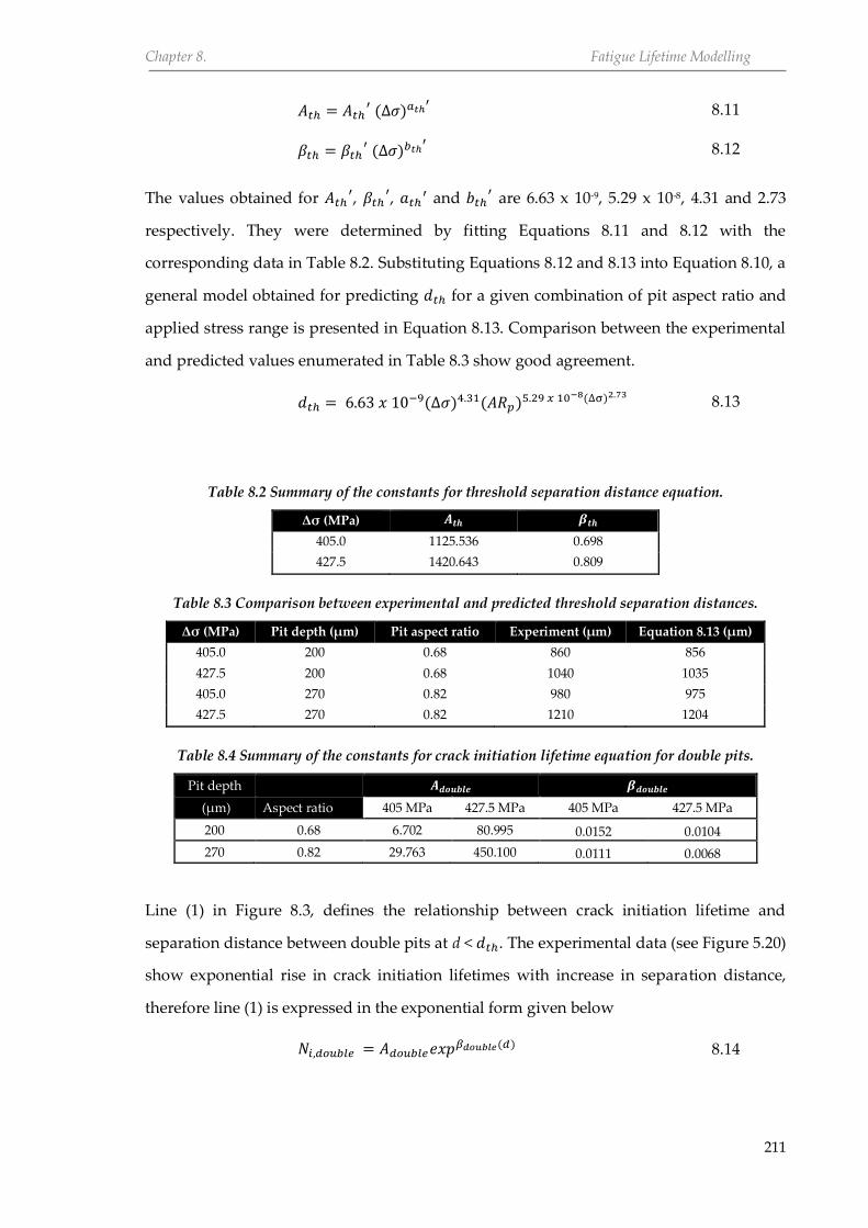
Chapter 8. Fatigue Lifetime Modelling
211
𝐴𝑡ℎ = 𝐴𝑡ℎ′ (∆𝜎)𝑎𝑡ℎ
′ 8.11
𝛽𝑡ℎ = 𝛽𝑡ℎ′ (∆𝜎)𝑏𝑡ℎ
′ 8.12
The values obtained for 𝐴𝑡ℎ′, 𝛽𝑡ℎ
′, 𝑎𝑡ℎ′ and 𝑏𝑡ℎ
′ are 6.63 x 10⁻⁹, 5.29 x 10⁻⁸, 4.31 and 2.73
respectively. They were determined by fitting Equations 8.11 and 8.12 with the
corresponding data in Table 8.2. Substituting Equations 8.12 and 8.13 into Equation 8.10, a
general model obtained for predicting 𝑑𝑡ℎ for a given combination of pit aspect ratio and
applied stress range is presented in Equation 8.13. Comparison between the experimental
and predicted values enumerated in Table 8.3 show good agreement.
𝑑𝑡ℎ = 6.63 𝑥 10−9(∆𝜎)4.31(𝐴𝑅𝑝)5.29 𝑥 10−8(∆σ)2.73 8.13
Table 8.2 Summary of the constants for threshold separation distance equation.
Δσ (MPa) 𝑨𝒕𝒉 𝜷𝒕𝒉
405.0 1125.536 0.698
427.5 1420.643 0.809
Table 8.3 Comparison between experimental and predicted threshold separation distances.
Δσ (MPa) Pit depth (µm) Pit aspect ratio Experiment (µm) Equation 8.13 (µm)
405.0 200 0.68 860 856
427.5 200 0.68 1040 1035
405.0 270 0.82 980 975
427.5 270 0.82 1210 1204
Table 8.4 Summary of the constants for crack initiation lifetime equation for double pits.
Pit depth 𝑨𝒅𝒐𝒖𝒃𝒍𝒆 𝜷𝒅𝒐𝒖𝒃𝒍𝒆
(µm) Aspect ratio 405 MPa 427.5 MPa 405 MPa 427.5 MPa
200 0.68 6.702 80.995 0.0152 0.0104
270 0.82 29.763 450.100 0.0111 0.0068
Line (1) in Figure 8.3, defines the relationship between crack initiation lifetime and
separation distance between double pits at d < 𝑑𝑡ℎ. The experimental data (see Figure 5.20)
show exponential rise in crack initiation lifetimes with increase in separation distance,
therefore line (1) is expressed in the exponential form given below
𝑁𝑖,𝑑𝑜𝑢𝑏𝑙𝑒 = 𝐴𝑑𝑜𝑢𝑏𝑙𝑒𝑒𝑥𝑝𝛽𝑑𝑜𝑢𝑏𝑙𝑒(𝑑) 8.14

Chapter 8. Fatigue Lifetime Modelling
212
where d is the centre-to-centre distance in µm, 𝑁𝑖,𝑑𝑜𝑢𝑏𝑙𝑒 is crack initiation lifetime for two
pits located close to another. 𝐴𝑑𝑜𝑢𝑏𝑙𝑒 and 𝛽𝑑𝑜𝑢𝑏𝑙𝑒 are material constants. Their values (see
Table 8.4) were determined from crack initiation lifetime-centre-to-centre distance
experimental data (see Appendix D) by regression analysis. Note that the subscripts
‘double’ indicate a variable or constant associated with two pits in proximity to each
other. Both constants can be observed to depend on pit size and stress. The constants
were first expressed as a function of pit aspect ratio as
𝐴𝑑𝑜𝑢𝑏𝑙𝑒 = 𝐴𝑑𝑜𝑢𝑏𝑙𝑒′ (𝐴𝑅𝑝)𝑎𝑑𝑜𝑢𝑏𝑙𝑒
′ 8.15
𝛽𝑑𝑜𝑢𝑏𝑙𝑒 = 𝛽𝑑𝑜𝑢𝑏𝑙𝑒′ (𝐴𝑅𝑝)𝑏𝑑𝑜𝑢𝑏𝑙𝑒
′ 8.16
where 𝐴𝑑𝑜𝑢𝑏𝑙𝑒′ , 𝛽𝑑𝑜𝑢𝑏𝑙𝑒
′ , 𝑎𝑑𝑜𝑢𝑏𝑙𝑒′ , and 𝑏𝑑𝑜𝑢𝑏𝑙𝑒
′ are constants, which were then expressed in
terms of stress range in Equations 8.17 - 8.20.
𝐴𝑑𝑜𝑢𝑏𝑙𝑒′ = 𝐴𝑑𝑜𝑢𝑏𝑙𝑒
′′ (∆𝜎) + 𝐶′ 8.17
𝛽𝑑𝑜𝑢𝑏𝑙𝑒′ = 𝛽𝑑𝑜𝑢𝑏𝑙𝑒
′′ (∆𝜎) + 𝐶′′ 8.18
𝑎𝑑𝑜𝑢𝑏𝑙𝑒′ = 𝑎𝑑𝑜𝑢𝑏𝑙𝑒
′′ (∆𝜎)𝑎′′ 8.19
𝑏𝑑𝑜𝑢𝑏𝑙𝑒′ = 𝑏𝑑𝑜𝑢𝑏𝑙𝑒
′′ (∆𝜎)𝑏′′ 8.20
where 𝐴𝑑𝑜𝑢𝑏𝑙𝑒′′ , 𝛽𝑑𝑜𝑢𝑏𝑙𝑒
′′ , 𝑎𝑑𝑜𝑢𝑏𝑙𝑒′′ , 𝑏𝑑𝑜𝑢𝑏𝑙𝑒
′′ , 𝑎′′, 𝑏′′, 𝐶′, and 𝐶′′ are all constants. Their values,
listed below, were obtained from non-linear regression analysis of the constants obtained
from Equations 8.15 and 8.16.
𝐴𝑑𝑜𝑢𝑏𝑙𝑒′′ = 116.80, 𝑎𝑑𝑜𝑢𝑏𝑙𝑒
′′ = 1.39 x 10⁻⁶, 𝑎′′ = 2.591, 𝐶′ = -47159
𝛽𝑑𝑜𝑢𝑏𝑙𝑒′′ = -1.62 x 10⁻⁴, 𝑏𝑑𝑜𝑢𝑏𝑙𝑒
′′ = -2.39 x 10⁻¹⁵, 𝑏′′= 5.693, 𝐶′′ = 7.35 x 10⁻²
Line (2) in Figure 8.3, defines the relationship between crack initiation lifetime and
separation distance between double pits at d ≥ 𝑑𝑡ℎ. Since this is a horizontal line with zero
slope, 𝑁𝑖,𝑑𝑜𝑢𝑏𝑙𝑒 will equate to the statistical distribution of crack initiation lifetime for a
single isolated pit, 𝑁𝑖,𝑠𝑖𝑛𝑔𝑙𝑒 . Thus, 𝑁𝑖,𝑑𝑜𝑢𝑏𝑙𝑒 in this region will be similar to the crack
initiation lifetime at d = 𝑑𝑡ℎ. This can be expressed as
𝑁𝑖,𝑑𝑜𝑢𝑏𝑙𝑒 = 𝐴𝑑𝑜𝑢𝑏𝑙𝑒𝑒𝑥𝑝𝛽𝑑𝑜𝑢𝑏𝑙𝑒(𝑑𝑡ℎ) 8.21
For a given combination of separation distance, pit aspect ratio and applied stress range,
𝑑𝑡ℎ was first calculated from Equation 8.13. The crack initiation lifetimes were then
predicted based upon Equations 8.14 when the given separation distance is less than the

Chapter 8. Fatigue Lifetime Modelling
213
predicted 𝑑𝑡ℎ and based upon Equation 8.21 when separation distance less than 𝑑𝑡ℎ.
Figures 8.4 and 8.5 show the predicted crack initiation lifetimes and the corresponding
experimental values. The numerical values are presented in Appendix D.
Experimental Ni,double
(cycles)
105 106 107
Pre
dic
ted N
i,d
ou
ble (
cyc
les)
105
106
107
Experimental Ni,double
(cycles)
105 106 107
Pre
dic
ted N
i,d
ou
ble (
cyc
les)
105
106
107
Figure 8.4 Comparison between experimental and predicted crack initiation lifetimes in air for 200
µm deep pits (aspect ratio = 0.68) loaded at (a) Δσ = 405MPa and (b) Δσ = 427.5.
(a)
± 25% error band
(b)
± 25% error band
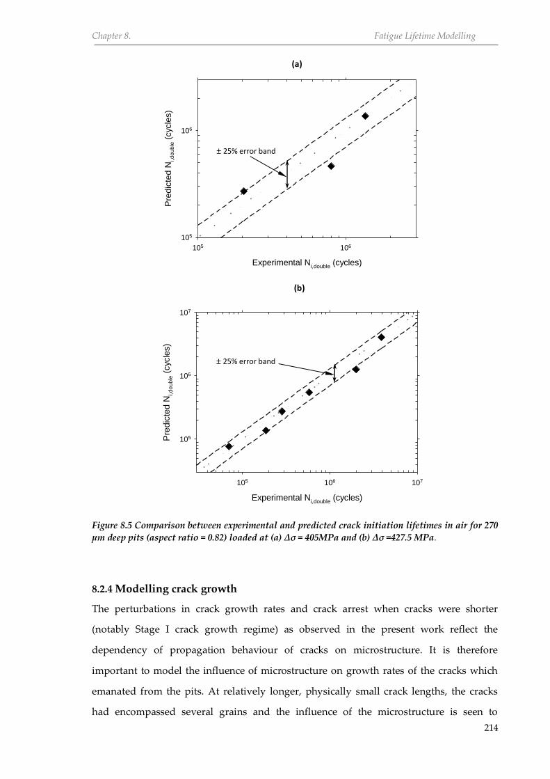
Chapter 8. Fatigue Lifetime Modelling
214
Experimental Ni,double
(cycles)
105 106
Pre
dic
ted N
i,do
ub
le (
cyc
les)
105
106
Experimental Ni,double
(cycles)
105 106 107
Pre
dic
ted N
i,do
ub
le (
cyc
les)
105
106
107
Figure 8.5 Comparison between experimental and predicted crack initiation lifetimes in air for 270
µm deep pits (aspect ratio = 0.82) loaded at (a) Δσ = 405MPa and (b) Δσ =427.5 MPa.
8.2.4 Modelling crack growth
The perturbations in crack growth rates and crack arrest when cracks were shorter
(notably Stage I crack growth regime) as observed in the present work reflect the
dependency of propagation behaviour of cracks on microstructure. It is therefore
important to model the influence of microstructure on growth rates of the cracks which
emanated from the pits. At relatively longer, physically small crack lengths, the cracks
had encompassed several grains and the influence of the microstructure is seen to
± 25% error band
± 25% error band
(a)
(b)

Chapter 8. Fatigue Lifetime Modelling
215
diminish (see Figure 5.31 – 5.35) because the crack has overcome the dominant barrier to
crack growth. In this regime (Stage II crack growth regime), the crack growth rate is an
increasing function of crack length. It is generally accepted that LEFM models cannot
provide accurate predictions of growth rates of cracks exhibiting these types of behaviour
due to the large plastic zone compared to the crack size [33, 82]. Hence, the
microstructural fracture mechanics and elastic-plastic fracture mechanics approaches,
based on the model developed by Hobson et al. [54] for in-air fatigue and later modified
by Akid et al. [36, 89, 183] for corrosion fatigue were adopted in the present work. These
models have been employed to successfully describe the discontinuous growth of short
cracks subject to perturbations arising from resistance of microstructural variables to
crack advance [36, 90, 183].
8.2.4.1 Short fatigue crack growth
According to these models, the propagation behaviour of microstructurally short (Stage I)
cracks can be expressed as
𝑑𝑎𝑠
𝑑𝑁 = 𝐶𝑠. (𝑑𝑖 − 𝑎𝑠) 8.22
where 𝑑𝑎𝑠
𝑑𝑁 is microstructurally short crack growth rate, d is the distance between adjacent
microstructural barriers to crack propagation, 𝑎𝑠 is the surface length of a short crack. 𝐶𝑠
is a material constant which depends on applied stress and environment and can be
expressed as
𝐶𝑠 = 𝐴𝑖. ∆𝜎𝛼𝑖 8.23
where 𝛥𝜎 is the applied stress range and 𝐴 and 𝛼 are also material constants. Combination
of Equations 8.22 and 8.23 yields the general Equation 8.24.
𝑑𝑎𝑠
𝑑𝑁 = 𝐴𝑖. ∆𝛾𝛼𝑖 . (𝑑𝑖 − 𝑎𝑠) for i =1,2......n 8.24
where i is the grain number and nth grain is the average number of grains which equates
the length of the dominant barrier. The constants were determined from experimental
data obtained in air and brine environments.
It is clear that the applicability of Equation 8.24 depends on the establishment of a
microstructural parameter, d, which describes the distance between successive barriers

Chapter 8. Fatigue Lifetime Modelling
216
and a dominant microstructural barrier, the dimensions of which represents the transition
crack length from a short crack growth to long crack growth regimes. Both are
determined by the material’s microstructure and may vary within the same material
depending on the texture. The in-air crack growth rate-crack length data in the regions
with decelerations in crack growth rates were analysed using linear regression analysis to
determine the value of d. The results showed a large variation that reflects the variation in
the material’s grain size suggesting that the values of the transition crack length and the
distances between successive barriers may vary between a range of values. This will relate
to the grain size distribution and actual grain sizes throughout the microstructure. The
transition length in air was estimated by considering the lengths of the observed non-
propagating cracks and the lengths obtained from experimental data. Since the
experimental data represents both short and long crack regimes, the point of inflexion of a
best fit third order polynomial fitted to the data was taken as a close approximation of the
transition length (see Figure 8.6). Table 8.5 shows that the estimated values of the
transition length range between 54 and 146 µm and its mean value is 105 µm.
Figure 8.6 Measured surface crack extension histories and fitted polynomials for different fatigue
tests conducted in air together with non-propagating cracks.
Table 8.5 Estimated values of Stage I to Stage transition length in air.
Δσ (MPa) Pit depth (µm) d (µm)
450 140 132
Non-propagating
cracks

Chapter 8. Fatigue Lifetime Modelling
217
414* 200 92
427.5 200 93
450 200 125
382.5* 270 54
405 270 128
427.5 270 71
450 270 146
* Non-propagating crack
The distances between successive barriers will likely tend toward the size of the largest
grains therefore, a representative value of 25 µm was adopted for the material and
subsequently used in crack growth data analysis. The mean value of the average
transition length (105 µm) was divided by this representative size of the largest grains (25
µm), to obtain n = 4 in Equation 8.24. The coefficient, 𝐶𝑠, in Equation 8.22 was determined
as the slope of plots of 𝑑𝑎𝑠
𝑑𝑁 versus 𝑑𝑖 − 𝑎𝑠 for each successive grain barrier and for each
crack that initiated from a pit. The obtained values are given in Table 8.6.
Table 8.6 Coefficients for short and long crack growth equations in air.
Δσ Short crack growth (𝑪𝒔𝒂 in Equation 8.22) Long crack growth
(𝑪𝒍𝒂 in Equation 8.25)
(MPa) 0 − 25 µ𝑚 25 − 50 µ𝑚 50 − 75 µ𝑚 75 − 100 µ𝑚 100 − 1300 µ𝑚
405 5.063 x 10⁻⁴ 5.063 x 10⁻⁴ 1.454 x 10⁻⁴ 1.090 x 10⁻⁴ 3.077 x 10⁻⁵
427.5 6.531 x 10⁻⁴ 6.531 x 10⁻⁴ 2.279 x 10⁻⁴ 1.133 x 10⁻⁴ 3.564 x 10⁻⁵
450 7.170 x 10⁻⁴ 7.170 x 10⁻⁴ 3.410 x 10⁻⁴ 1.166 x 10⁻⁴ 4.021 x 10⁻⁵
Due to limited experimental data points for crack lengths less than 25 µm, sensible values
could not be obtained for the coefficients for the first grain barrier, 𝑑1. Hence, for analysis
purposes, the coefficients obtained for the second barrier i.e. 𝑑2 were also assumed to be
applicable for 𝑑1. The variations that can be seen in the values of 𝐶𝑠 at the same stress level
indicate that the crack growth rates in different grains are not necessarily the same at a
given stress level. This expected because the growth rate of an individual crack will
depend on the size of the grain in which it is growing and the orientation of the grain’s
slip plane and slip direction with respect to the loading axis. 𝐶𝑠 was expressed as a
function of applied stress range by non-linear regression analysis of the 𝐶𝑠-Δσ data in
Table 8.6 to obtain the constants in Equation 8.24. The values of the constants are:
𝐴𝑖 = 1.18 x 10⁻¹², 1.16x 10⁻²⁵ and 2.33 x 10⁻⁶ (for grains 2 – 4 respectively)
and 𝛼𝑖 = 3.315, 8.092 and 0.640 (for grains 2 – 4 respectively)

Chapter 8. Fatigue Lifetime Modelling
218
with 𝑑𝑖 = 25, 50, 75 and 100 µm.
The crack growth rates in this regime were calculated for air fatigue by substituting the
values of these constants in to Equation 8.24. The results, plotted together with
experimental data, are shown in Figure 8.7.
For corrosion fatigue conditions, there appears to also be perturbations in observed crack
growth rates although not as marked as in air. In order to be able to model the growth
behaviour of corrosion fatigue short cracks, it was assumed that once a crack initiates
from a pit, the microstructure also influences propagation behaviour. Unfortunately there
were insufficient experimental data points for determining 𝐶𝑠 at different stress levels
hence, 𝐴𝑖 and 𝛼𝑖 could also not be determined experimentally. Since the growth rates of
the short cracks were higher in the aggressive environment than in air, a conservative
approach that adopted for modelling crack growth in this regime, was to increase the
values of 𝐶𝑠 obtained in air by a specific factor. This factor should correlate with the
difference in the number cycles taken to propagate a short crack beyond the dominant
microstructural barrier in corrosion fatigue compared to air. From comparative inspection
of experimental crack length-number of cycles data obtained in air and corrosion fatigue,
an average value of 2 seemed appropriate. Therefore, the values obtained for the
constants are:
𝐴𝑖 = 2.95 x 10⁻¹², 2.89 x 10⁻²⁵ and 5.84 x 10⁻⁶ (for grains 2 – 4 respectively)
and 𝛼𝑖 = 3.315, 8.092 and 0.640 (for grains 2 – 4 respectively)
The crack growth rates in corrosion fatigue were calculated using these values for the
constants in Equation 8.24. The results are plotted together with experimental results as
shown in Figure 8.8.

Chapter 8. Fatigue Lifetime Modelling
219
Crack length (m)
10 100 1000
Cra
ck g
row
th r
ate
(m
/cyc
le)
10-10
10-9
10-8
10-7
Experimental
Model
Crack length (m)
10 100 1000
Cra
ck g
row
th r
ate
(m
/cyc
le)
10-10
10-9
10-8
10-7
Experimental
Model
Crack length (m)
10 100 1000
Cra
ck g
row
th r
ate
(m
/cyc
le)
10-10
10-9
10-8
10-7
Experimental
Model
Δσ = 405 MPa, 𝒅𝒑 = 140 µm, 𝑨𝑹𝒑 = 𝟎. 𝟓𝟐
Δσ = 427.5 MPa, 𝒅𝒑 = 200 µm, 𝑨𝑹𝒑 = 𝟎. 𝟔𝟖
(a)
(b)
Δσ = 427.5 MPa, 𝒅𝒑 = 270 µm, 𝑨𝑹𝒑 = 𝟎. 𝟖𝟐
(c)
Eqn 8.24
Eqn 8.27
Eqn 8.24
Eqn 8.27
Eqn 8.27
Eqn 8.24

Chapter 8. Fatigue Lifetime Modelling
220
Crack length (m)
10 100 1000
Cra
ck g
row
th r
ate
(m
/cyc
le)
10-10
10-9
10-8
10-7
Experimental
Model
Crack length (m)
10 100 1000
Cra
ck g
row
th r
ate
(m
/cyc
le)
10-10
10-9
10-8
10-7
Experimental
Model
Crack length (m)
10 100 1000
Cra
ck g
row
th r
ate
(m
/cyc
le)
10-10
10-9
10-8
10-7
Experimental
Model
Figure 8.7 Comparison of predicted and experimental fatigue crack growth rates in air.
Δσ = 450 MPa, 𝒅𝒑 = 140 µm, 𝑨𝑹𝒑 = 𝟎. 𝟓𝟐
Δσ = 450 MPa, 𝒅𝒑 = 200 µm, 𝑨𝑹𝒑 = 𝟎. 𝟔𝟖
Δσ = 450 MPa, 𝒅𝒑 = 270 µm, 𝑨𝑹𝒑 = 𝟎. 𝟖𝟐
(d)
(e)
(f)
Eqn 8.27
Eqn 8.27
Eqn 8.27
Eqn 8.24
Eqn 8.24
Eqn 8.24

Chapter 8. Fatigue Lifetime Modelling
221
Crack length (m)
10 100 1000
Cra
ck g
row
th r
ate
(m
/cyc
le)
10-10
10-9
10-8
10-7
Experimental
Model
Crack length (m)
10 100 1000
Cra
ck g
row
th r
ate
(m
/cyc
le)
10-10
10-9
10-8
10-7
Experimental
Model
Crack length (m)
10 100 1000
Cra
ck g
row
th r
ate
(m
/cyc
le)
10-10
10-9
10-8
10-7
Experimental
Model
(a)
(c)
(b)
Δσ = 427.5 MPa, 𝒅𝒑 = 270 µm, 𝑨𝑹𝒑 = 𝟎. 𝟖𝟐
Δσ = 427.5 MPa, 𝒅𝒑 = 200 µm, 𝑨𝑹𝒑 = 𝟎. 𝟔𝟖
Δσ = 405 MPa, 𝒅𝒑 = 270 µm, 𝑨𝑹𝒑 = 𝟎. 𝟖𝟐
Eqn 8.24
Eqn 8.24
Eqn 8.24
Eqn 8.27
Eqn 8.27
Eqn 8.27

Chapter 8. Fatigue Lifetime Modelling
222
Crack length (m)
10 100 1000
Cra
ck g
row
th r
ate
(m
/cyc
le)
10-10
10-9
10-8
10-7
Experimental
Model
Crack length (m)
10 100 1000
Cra
ck g
row
th r
ate
(m
/cyc
le)
10-10
10-9
10-8
10-7
Experimental
Model
Crack length (m)
10 100 1000
Cra
ck g
row
th r
ate
(m
/cyc
le)
10-10
10-9
10-8
10-7
Experimental
Model
Figure 8.8 Comparison of predicted and experimental crack growth rates in corrosion fatigue.
(d)
(f)
(e)
Δσ = 450 MPa, 𝒅𝒑 = 270 µm, 𝑨𝑹𝒑 = 𝟎. 𝟖𝟐
Δσ = 450 MPa, 𝒅𝒑 = 200 µm, 𝑨𝑹𝒑 = 𝟎. 𝟔𝟖
Δσ = 450 MPa, 𝒅𝒑 = 140 µm, 𝑨𝑹𝒑 = 𝟎. 𝟓𝟐
Eqn 8.27
Eqn 8.24
Eqn 8.24
Eqn 8.24
Eqn 8.27
Eqn 8.27

Chapter 8. Fatigue Lifetime Modelling
223
8.2.4.2 Long fatigue crack growth
In the long crack growth regime, there is little or no influence of microstructure on crack
growth hence, the crack growth rates increase continuously with crack length. The
propagation rate of the cracks in this regime can be expressed as
𝑑𝑎𝑙
𝑑𝑁 = 𝐶𝑙𝑎 . 𝑎𝑙 − 𝐷𝑙
8.25
where 𝑑𝑎𝑙
𝑑𝑁 is long crack growth rate and 𝐷𝑙 is a stress dependent crack growth rate
threshold. 𝐶𝑙𝑎 is stress and environment dependent material constant that may be
expressed as
𝐶𝑙𝑎 = 𝐵. ∆𝜎𝛽 8.26
where 𝛥𝜎 is the applied stress range and B and 𝛽 are material constants.
Substituting Equation 8.26 into Equation 8.25 yields the general Equation 8.27.
𝑑𝑎𝑙
𝑑𝑁 = 𝐵. ∆𝜎𝛽 . 𝑎𝑠 − 𝐷𝑙 8.27
The values of the coefficient, 𝐶𝑙𝑎, at different stress levels were first determined as the
slopes of crack growth rates-crack length data for crack lengths greater than 𝑑𝑡𝑟 in air and
corrosion fatigue i.e. 100 µm (see Table 8.6 for the values of 𝐶𝑙𝑎). Non-linear regression
analysis was then conducted on the Δσ-𝐶𝑙𝑎data to obtain the constants in Equation 8.27. In
air and corrosion fatigue, the values obtained for B and β are 7.301 x 10⁻¹² and 2.542 and
7.604 x 10⁻¹⁹ and 5.240 respectively.
The constant,𝐷𝑙, represents a minimum threshold crack growth rate that is dependent on
the stress range at which the crack growth rate approaches zero. 𝐷𝑙 was therefore
calculated from the fatigue limit by employing the following equation
𝐷𝑙 = 𝐵. (∆𝜎0)𝛽𝑑𝑡𝑟 8.28
where ∆𝜎0 is the fatigue limit.
Since the experimental results showed that the fatigue limit in air is a function of pit size,
different 𝐷𝑙 values were obtained for different pit sizes. The values obtained in air are
given in Table 8.7. To determine the fatigue limit in corrosion fatigue, a trendline was
applied to the corrosion fatigue S-N data. The fatigue limit for each pit size was then

Chapter 8. Fatigue Lifetime Modelling
224
evaluated as the point of intersection at 107 cycles. These were 200, 160 and 140 MPa for
pit aspect ratios of 0.52, 0.68 and 0.82 respectively. Although there appears to be
dependence between both, it is expected that this limiting stress range will be
independent of pit size at these lower stress ranges due to the dominance of corrosion
over that of mechanical damage. Moreover, the difference between predicted number of
cycles at highest – 200 MPa and lowest – 140 MPa stress ranges predicted from the model
is generally less than 3%. Hence, a single value of 140 MPa was adopted as a conservative
fatigue limit of this material in the aggressive environment. This was used to determine
the value of 𝐷𝑙 for corrosion fatigue crack growth (see Table 8.7).
Table 8.7 Calculated values of 𝐷𝑙 for different pit sizes in air and corrosion fatigue.
Pit depth (µm) Aspect ratio Δσ0 (MPa) 𝑫𝒍 (µm/cycle)
Air
𝑫𝒍 (µm/cycle)
Corrosion fatigue
140 0.52 436.5 3.733 x 10⁻³ 1.339 x 10⁻⁵
200 0.68 414.0 3.264 x 10⁻³ 1.339 x 10⁻⁵
270 0.82 382.5 2.667 x 10⁻³ 1.339 x 10⁻⁵
The crack growth rates in this regime, which were calculated using Equation 8.27, are also
shown in Figure 8.7 for air and in Figure 8.8 for corrosion fatigue.
8.2.4.3 Crack propagation lifetimes calculations
The individual lifetimes spent in the short and long crack regimes in air and corrosion
fatigue were calculated by integrating Equation 8.23 in the range 0 to 100 µm. Likewise,
the number of cycles spent in the long crack regime were calculated by integrating
Equation 8.27 in the range 100 µm to the final crack length, 𝑎𝑓. Experimentally, 𝑎𝑓 was
observed for the majority of the tests to be approximately 1300 µm. The crack propagation
lifetimes were then obtained by adding these individual lifetimes. A comparison between
experimental and predicted crack propagation lifetimes is presented in Figure 8.9a for air
and Figure 8.9b for corrosion fatigue. It can be observed that the model predictions show
good agreement with experimental data.
(a)

Chapter 8. Fatigue Lifetime Modelling
225
Experimental Np (cycles)
105
Pre
dic
ted N
p (
cyc
les)
105
= 405 MPa, dp = 270 m
= 427.5 MPa, dp = 200 m
= 427.5 MPa, dp = 270 m
= 450 MPa, dp = 140 m
= 450 MPa, dp = 200 m
= 450 MPa, dp = 270 m
Experimental Np (cycles)
105
Pre
dic
ted N
p (
cyc
les)
105
= 405 MPa, dp = 270 m
= 427.5 MPa, dp = 200 m
= 427.5 MPa, dp = 270 m
= 450 MPa, dp = 200 m
= 450 MPa, dp = 270 m
Figure 8.9 Comparison between experimental and predicted crack propagation lifetimes in (a) air
and (b) corrosion fatigue.
8.2.5 Fatigue lifetime predictions
The total lifetime was obtained as the sum of the lifetimes spent propagating damage in
each of the individual regimes applicable to air (Equation 8.29) and corrosion fatigue
(Equation 8.30).
± 20% error band
± 20% error band
(b)
2
3
2
3
4
4
3 x10⁴
4 5
6
7
8
9
4
5
6
7
8
9

Chapter 8. Fatigue Lifetime Modelling
226
𝑁𝑎𝑓 = 𝑁𝑝𝑡𝑐 + 𝑁𝑠𝑐 + 𝑁𝑙𝑐 8.29
𝑁𝑐𝑓 = 𝑁𝑝𝑔 + 𝑁𝑝𝑡𝑐 + 𝑁𝑠𝑐 + 𝑁𝑙𝑐 8.30
The predicted lifetimes in each regime and their summation i.e. fatigue lifetimes are
summarised in Table 8.8 for air and in Table 8.9 for corrosion fatigue.
Table 8.8 Comparison between experimental and predicted air fatigue lifetimes.
Δσ
(MPa)
𝒅𝒑
(µm)
𝑨𝑹𝒑
𝑵𝒑𝒕𝒄 (cycles)
Eqn. 8.9
𝑵𝒔𝒄 (cycles)
Eqn. 8.24
𝑵𝒍𝒄 (cycles)
Eqn. 8.27
Predicted
lifetime
Experimental
lifetime
405 140 0.52 28134266 - - 28134266 > 10000000
427.5 140 0.52 7831872 - - 7831872 > 10000000
450 140 0.52 2598558 42314 126117 2766989 2400000
405 200 0.68 11142619 - - 11142619 > 10000000
427.5 200 0.68 3834830 49069 142217 4026116 4603000
450 200 0.68 1487404 42314 100569 1630287 1514000
405 270 0.82 5838120 59143 143398 6040661 5205000
427.5 270 0.82 2329835 49069 108126 2487030 3655000
Table 8.9 Comparison between experimental and predicted corrosion fatigue lifetimes.
Δσ
(MPa)
𝒅𝒑
(µm)
𝑨𝑹𝒑
𝑵𝒑𝒈 (cycles)
Eqn. 8.5
𝑵𝒑𝒕𝒄 (cycles)
Eqn. 8.9
𝑵𝒔𝒄 (cycles)
Eqn. 8.24
𝑵𝒍𝒄 (cycles)
Eqn. 8.27
Predicted
lifetime
Experimental
lifetime
405 140 0.52 7165 765572 29497 73357 875591 889000
427.5 140 0.52 6977 490558 24890 55240 577665 669000
450 140 0.52 6795 325066 21709 42210 395780 431300
405 200 0.68 12455 451625 29497 73357 566934 651000
427.5 200 0.68 12130 304255 24890 55240 396514 396000
450 200 0.68 11812 210497 21709 42210 286229 265000
405 270 0.82 19835 312479 29497 73357 435168 447000
427.5 270 0.82 19316 218003 24890 55240 317449 341000
405 140 0.52 18811 155432 21709 42210 238162 249000
8.3 Discussion
Empirical models for predicting fatigue lifetimes of pre-pitted specimens in air and
corrosion fatigue were developed in this work. The lifetime models attempt to quantify
damage at different stages of the fatigue process viz pit growth, pit-to-crack transition,
short crack growth and long crack growth in air and in an aggressive environment. By
accumulating the lifetimes spent in each of these regimes, the overall lifetimes have been
calculated. Experimental results showed that lifetime to crack initiation depend on
applied stress, pit size and environment. The model accounts for these factors thus, the

Chapter 8. Fatigue Lifetime Modelling
227
crack pit-to-crack transition lifetimes can be predicted for a given combination of applied
stress range and pit size in air or in corrosion fatigue. The predicted lifetimes presented in
Figure 8.2 show good agreement with experimental data. A special case of crack initiation
behaviour was also modelled where the crack initiation lifetime, for samples containing
double pits in close proximity, can also be predicted for a known combination of pit size,
and stress range and separation distance between two pits. It can be observed from
Figures 8.4 and 8.5 that the model predictions show good agreement with experimental
data. The disparities between both sets of data may be attributed to inaccuracies in
determining the 𝑑𝑡ℎ values, which were only estimated from experimental data. With
sufficient experimental data points and for a wider range of stress range and pit aspect
ratio, the model can be improved to provide more accurate predictions.
After initiation, the cracks propagate through in the so-called ‘short crack regime’ where
the growth rates of the cracks show perturbations due to the effect of the microstructure.
The model accounts for this effect by modelling deceleration of crack growth rate. After
progressing beyond the dominant microstructural barrier, the effect of the microstructure
diminishes and cracks were assumed to behave as long cracks. The model also predicts
the growth rates of the cracks in this long crack regime based on the fatigue limit for a
given pit size. In the aggressive environment, the crack growth rates are faster than in air,
thereby resulting in shorter lifetimes in both short and long crack regimes. The crack
growth curves generated using the short and long crack growth models, Figures 8.7 and
8.8 respectively, as well as the predicted crack propagation lives, Figure 8.9 all show good
correlation with experimental data.
By accumulating the individual lifetimes spent to initiate a crack and propagate the crack
through the short and long crack regimes to failure, total fatigue lifetime in air was
predicted (see Figure 8.10a). In corrosion fatigue, the overall fatigue lifetime was
predicted by summation of the individual lifetimes spent in the individual regimes
described above, see Figure 8.10b. The predicted lifetimes showed good agreement with
experimental data.

Chapter 8. Fatigue Lifetime Modelling
228
Experimental lifetimes (cycles)
105 106 107
Pre
dcited lifetim
es (
cyc
les)
105
106
107
Experimental lifetimes (cycles)
105 106
Pre
dcited lifetim
es (
cyc
les)
105
106
Figure 8.10 Comparison of experimental and predicted fatigue lifetimes in (a) air and (b) corrosion
fatigue.
±20 error band
(b)
(a)
±20 error band

Chapter 9
General Discussion

Chapter 9. General Discussion
230
9.1 Introduction
The fatigue and corrosion fatigue behaviour of API 5L X-65 HSLA linepipe steel has been
investigated by both experimental and modelling techniques. Results and discussions for
the experimental studies were presented in Chapter 5 while those relating to finite
element analysis and cellular automata finite element model development were reported
in Chapter 6 and Chapter 7 respectively. The objective of this chapter is to present a
general discussion of the overall objectives of this research, while taking into account
evidence from each of the experimental (Chapter 5) and modelling (Chapter 6 and
Chapter 7) studies.
9.2 The fatigue limit
From in-air tests conducted on plain specimens, a limiting stress range was observed
below which cracks did not initiate, therefore the specimens did not fail. This plain
specimen fatigue limit was evaluated to be Δσ = 450 MPa. However, at stress levels below
this stress range, it was found that cracks were still able to initiate and propagate when
pits were present on the specimens, thus suggesting a reduction in the plain specimen
fatigue limit. Observations showed that a limiting stress also exists below which cracks
either did not initiate from a pit, or if initiated, became non-propagating. The fatigue limit
was previously related to a safe stress range below which cracks do not initiate, hence
there will be no failure. However, based on the knowledge of the fatigue limit is not a
consequence of non-initiation of cracks but related with the materials ability to arrest an
initiated crack at this stress range [36, 58, 86, 90]. Therefore, the fatigue limit of metals has
been described as the stress range below which cracks may initiate but do not propagate.
This limiting stress range was found to decrease with increasing pit size (based on
uniaxial loading conditions employed in the tests).
Cracks can become non-propagating when the mechanical driving force at the crack tip is
not sufficient for continued crack propagation. Further investigations suggest that the
arrest of cracks was most likely due to the resistance of the microstructure, the stress
intensity factor range associated with the crack being below the threshold level required
for continued crack propagation or a combination of both. In the inert environment, crack

Chapter 9. General Discussion
231
tips were arrested at ferrite-ferrite grain boundaries whereas no crack arrests were
observed for tests carried out in aggressive environment despite testing at stress levels
well below that at which cracks arrested in air. The ability of the non-propagating cracks
to re-propagate to failure at the previous in-air fatigue limit after (i) increasing the crack
size by cycling at a higher stress level for a very short period and/or (ii) introducing an
aggressive environment, all be it temporarily, showed an elimination of the pitted
specimen fatigue limit. In practice, a momentary transient of the stress range above the in-
air fatigue limit (overload) can increase the length of cracks that previously initiated from
a pit but had arrested, and thereby increase the associated stress intensity factor.
Introduction of the environment may also effectively increase the crack size and/or or
reduce the resistance of the microstructural barrier. In both the above cases, arrested
cracks are able to re-propagate. Therefore, it can be argued that the adoption of the in-air
fatigue limit as a safe operating stress range may only be valid if the operating conditions
exclude any possibility of overloads or aggressive environments.
In contrast to in-air tests, non-propagating cracks were not observed in corrosion fatigue
tests and there appeared to be no apparent fatigue limit at stress ranges as low as 300
MPa. In other words, once cracks initiated, they were able to propagate until failure of the
samples. This highlights the influence an aggressive operating environment can have on
the fatigue properties of materials, notably a reduction of a safe operating stress range.
Although the present study showed that the non-propagating crack re-propagated when
the aggressive environment was introduced, it does not mean that cracks emanating from
pits cannot stop propagating in the presence of an aggressive environment as found in
some material-environment systems [9, 195, 209].
9.3 Influence of pit size on fatigue strength
Stress-life curves, particularly for tests carried out in air (see Figure 5.47), show that
fatigue strength is dependent on pit size. Figure 9.1 reveals that, for the present loading
conditions, the fatigue strength (plotted as a factor of the plain fatigue limit) reduces with
increase in pit size, but only for pit sizes greater than a critical value. This value is
estimated from the plot to be 110 µm, suggesting that the fatigue strength should be
independent of a pit with depth less than 110 µm. To verify this assertion, an additional

Chapter 9. General Discussion
232
test was carried out on a pre-pitted specimen with a pit depth of 90 µm, loaded at Δσ =
450 MPa (i.e. the plain specimen fatigue limit). The aspect ratio of the pit was 0.43. As
indicated on Figure 9.1 (‘Additional test’), no cracks initiated from this pit size hence, it
had no effect on the plain fatigue strength.
From a practical viewpoint and from the above, prediction of the effect of small defects
such as pits on the fatigue strength of structural components is important for design and
lifetime assessment [31, 308]. Two existing models are the fatigue notch factor and
fracture mechanics approaches discussed below.
Pit depth (m)
0 50 100 150 200 250 300
FL
_p
re-p
itte
d/
FL
_p
lain
0.8
0.9
1.0
Aspect ratio
0.0 0.2 0.4 0.6 0.8 1.0
Pit depth
Aspect ratio
Figure 9.1 Fatigue strength reduction factor as a function of depth and pit aspect ratio.
Assessment of pits as notches
This approach assumes that corrosion pits are equivalent to notches due to their
geometric discontinuity effect on stress distribution i.e. stress gradient so that the notch
factor, 𝐾𝑓, defined as the ratio of the fatigue strength of plain specimen to that of a
notched (pre-pitted) specimen at 107 cycles, can be determined. The question in debate is:
are pits equivalent to notches in terms of their effects on fatigue strength?. In order to
answer this, a comparison was made between experimental, 𝐾𝑓, and those calculated
using fracture mechanics models, 𝐾𝑓′. Here the pits were assumed to be blunt notches
since their elastic stress concentration factors are less than 3 [309, 310].
Additional test
Plain fatigue limit

Chapter 9. General Discussion
233
𝐾𝑓′ was calculated using empirical models developed by Peterson [311, 312] (Equation 9.1)
and Smith and Miller [313] (Equation 9.2).
𝐾𝑓′ = 1 +
𝐾𝑇−1
1+ 𝛹 𝑟⁄ (9.1)
𝐾𝑓′ = [1 + 4.67√
𝑎
𝑟]
1
2
(9.2)
where a is the notch depth and r is the notch root radius. 𝛹 is a material constant
calculated to be 226 µm using Equation 9.3 [310] and KT is the stress concentration factor
obtained from finite element analysis.
𝛹 = 0.0254 (2067
𝑆𝑈𝑇𝑆)
1.8
(9.3)
where 𝑆𝑈𝑇𝑆 is ultimate tensile stress (620 MPa for X65 steel).
The calculated fatigue notch factors plotted as a function of pit depth in Figure 9.2
generally show the same trend as the experimental data i.e. increase with pit depth,
indicating that the pit depth governs the fatigue behaviour. However, the models did not
correlate well with the experimental data; the former being generally greater than the
latter by as much as a factor of approximately 1.9. This suggests that assessing these pits
as blunt notches will overestimate their effect on fatigue strength. This overestimation
agrees with previous studies [123]. Moreover, the observation of non-propagating cracks
from pits does not agree with a characteristic of blunt notches, which is that, the initiation
and propagation threshold stresses are the similar so that initiated cracks are able to
propagate at the same stress level [314]. If the pits are equivalent to blunt notches, then
the stress level for initiation should also be sufficient to propagate the initiated crack until
failure. Hence, there should be no non-propagating cracks.
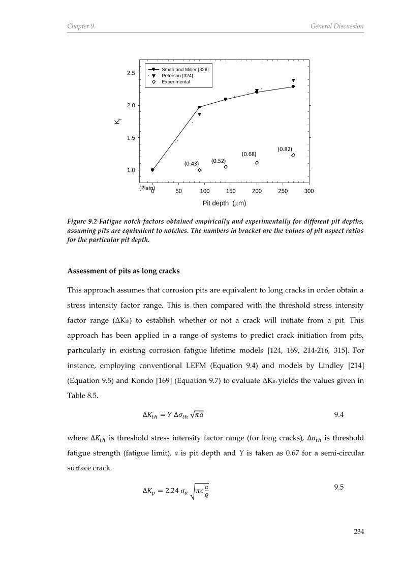
Chapter 9. General Discussion
234
Pit depth (m)
0 50 100 150 200 250 300
Kf
1.0
1.5
2.0
2.5Smith and Miller [326]
Peterson [324]
Experimental
Figure 9.2 Fatigue notch factors obtained empirically and experimentally for different pit depths,
assuming pits are equivalent to notches. The numbers in bracket are the values of pit aspect ratios
for the particular pit depth.
Assessment of pits as long cracks
This approach assumes that corrosion pits are equivalent to long cracks in order obtain a
stress intensity factor range. This is then compared with the threshold stress intensity
factor range (ΔKth) to establish whether or not a crack will initiate from a pit. This
approach has been applied in a range of systems to predict crack initiation from pits,
particularly in existing corrosion fatigue lifetime models [124, 169, 214-216, 315]. For
instance, employing conventional LEFM (Equation 9.4) and models by Lindley [214]
(Equation 9.5) and Kondo [169] (Equation 9.7) to evaluate ΔKth yields the values given in
Table 8.5.
∆𝐾𝑡ℎ = 𝑌 ∆𝜎𝑡ℎ √𝜋𝑎 9.4
where ∆𝐾𝑡ℎ is threshold stress intensity factor range (for long cracks), ∆𝜎𝑡ℎ is threshold
fatigue strength (fatigue limit), a is pit depth and Y is taken as 0.67 for a semi-circular
surface crack.
∆𝐾𝑝 = 2.24 𝜎𝑎 √𝜋𝑐𝛼
𝑄 9.5
(0.52) (0.68)
(0.82)
(Plain)
(0.43)

Chapter 9. General Discussion
235
where ∆𝐾𝑝 is critical pit condition (equivalent to ΔKth), 𝜎𝑎 is half threshold stress range, c
is half pit diameter, 𝛼 is pit aspect ratio and Q is given by
𝑄 = 1 + 1.464 𝛼1.65 9.6
𝐾𝑡ℎ =
∆𝜎𝑡ℎ√(𝜋𝑎)[1.13 − 0.07𝛼0.5]
[1 + 1.47𝛼1.64]0.5
9.7
The changes in ΔKth values as a result of changes in pit depth indicate a clear breakdown
of the application of LEFM conditions to the pits. This is because, under small scale
yielding conditions and with no influence of microstructure, ΔKth should be nominally
independent of crack length [94, 316] (pit size in this case), which is clearly not the case in
the present work. This highlights the difficulty and inaccuracy in applying this approach
for assessing whether or not cracks will initiate from pits. It is therefore expected that
predictions based on this approach will lead to over-conservative lifetime models.
Table 9.1 Calculated threshold stress intensity factor range as a function of pit depth and pit
aspect ratio.
Pit depth (µm) Aspect ratio Fatigue limit (MPa) Eq. (9.4) Eq. (9.5) Eq. (9.7)
90 0.38 450 5.07 6.92 7.44
140 0.52 436.5 6.13 7.76 6.72
200 0.68 414 6.95 8.05 5.85
270 0.82 382.5 7.46 8.61 5.03
Assessment of pits as short cracks
Considering the dependence of the fatigue limit on pit size (see Figure 9.1), the influence
of microstructure leading to crack arrest, and the plastic fields around the pit sizes
employed in the present study, it is sensible to consider pits to be equivalent to short
cracks. The Kitagawa-Takahashi model describes the variation of the limiting threshold
stress that will cause crack initiation, crack arrest or fatigue failure with known pre-
existing crack size, in this case pit size. Based on the empirical relationship proposed by
El-Hadad and co-workers (Equation 9.8) [92] by defining an intrinsic defect size (in the
present case pit size), 𝑎0, for estimating the threshold stress intensity factor range for
small defects, the limiting condition for pit size effect on the fatigue strength can be
captured. Although the physical meaning of the intrinsic defect size is not well
understood, its applicability to pits has been demonstrated [9, 123, 215, 317]. With a ∆𝐾𝑡ℎ

Chapter 9. General Discussion
236
value of 8 MPa√m, 𝑎0 was evaluated from Equation 9.9 as 220 µm. This intrinsic pit size is
appreciably larger than any microstructural characteristics; hence cannot be related to the
material’s microstructure.
∆𝐾𝑡ℎ = 𝑌 ∆𝜎𝑡ℎ √𝜋(𝑎 + 𝑎0) (9.8)
𝑎0 = 1
𝜋(
∆𝐾𝑡ℎ
𝑌∆𝜎𝐹𝐿)
2
(9.9)
The applicability of the assessment of pits as short cracks is illustrated in a Kitagawa type
diagram (Figure 9.3). The curve calculated from Equation 9.8 predicts the transition
between the two limiting conditions i.e. ∆𝜎𝐹𝐿 and ∆𝐾𝑡ℎ . As the pit depth increases, the
fatigue strength decreases progressively from the plain fatigue limit towards that
predicted from Equation 9.4, i.e. deeper pits greater than 1mm can be treated as long
cracks. Although the curve underestimates the effect of pit size on fatigue strength, it
provided a better approximation than when the pits are considered as blunt notches and
long cracks.
Pit depth (m)
101 102 103
Str
ess r
ange (
MP
a)
102
103
Figure 9.3 Kitagawa type diagram illustrating the effect of pit depth on the fatigue limit.
9.4 Effect of stress on pit development
The pit growth regime constitutes an important time-dependent stage in corrosion fatigue
systems, where pits are precursors to cracking. The rate of pit growth may be considered
to be influenced mainly by material properties, local solution chemistry and stress state.
𝜎𝐹𝐿 = constant
Eqn. 9.4
Eqn. 9.8

Chapter 9. General Discussion
237
Some previous studies have shown that pit growth rate can be influenced by the
magnitude of applied stress [117, 124, 250], while other studies suggested that this effect
may depend on the degree of plasticity around the pit [127, 250, 318]. Experimental results
from the present work revealed that cyclic stress promotes local kinetics of dissolution
occurring in the pit by increasing the rate of metal loss, thus increasing the rate of pit
growth. The influence of applied stress on localised dissolution rate is attributed to strain-
assisted dissolution [89, 90]. To offer more insight into this mechanism, the interaction
between local kinetics in the pit and applied stress was investigated by employing a 2-D
CAFE model. The results of this model, which employs an empirical model to account for
the effect of stress on localised corrosion, are consistent with experimental results (see
Figure 7.11) and give more credence to the role of stress in pit development i.e. increased
dissolution rate which in turn results in faster pit growth rate.
A notable observation in the present study is the disparity between the plots of pit depth
versus time with and without stress, which increased as the pits become deeper (greater
aspect ratio) with time (see Figure 5.11). This behaviour was attributed to the strain
localisation effect of a pit, in that the level of localised strain associated with a growing pit
should also increase with time. Firstly, it was confirmed from 3-D FE analysis and from
the 2-D CAFE model that the extent of strain localization increases with pit depth and
with time. This implies that deeper pits would have a relatively greater level of local and
possibly plastic strain if the yield strain is exceeded. It is noted here that the changing
parameter is not applied stress but the size of the pit. Considering that in the mechanism
of strain-assisted dissolution, the extent of the effect of strain on dissolution kinetics
would be proportional to the level of localised strain, it is proposed that a growing pit
(increasing size) will further promote dissolution of the pit’s surrounding matrix due to
its associated localised strain. Therefore, the resultant effect of this process would be an
increase in metal loss under applied stress compared to the unstressed case. Moreover,
the region of the pit where the plastic strain is highest will likely be the most susceptible
to slip dissolution [305], which may have implications for crack nucleation.
The present results show that the strain localization effect of a pit is, not only
mechanistically important for crack initiation, but also influences the rate of pit growth
significantly. An increase in the pit growth rate as a result of increased stress will lead to a
decrease in the fraction of lifetime spent in the pitting regime, prior to the pit-to-crack

Chapter 9. General Discussion
238
transition, thereby shortening corrosion fatigue lifetime. Similarly, lowering the applied
stress will increase this period because it will require a longer time to develop a pit that is
sufficiently deep to promote crack initiation. In the present system where pits are taken to
be the precursors to cracks, consideration of the relationship between pit growth rate and
applied stress is of great importance for the development of realistic corrosion fatigue
models. Therefore, the effect of applied stress was accounted for in the empirical pit
growth model proposed in Equation 8.5. Previous studies have shown that the
relationship between stress and pit growth can be linear or non-linear [124, 250]. For the
present study, it cannot be concluded whether the contribution of stress to pit growth for
the present material-environment system is linear or not since test was conducted at only
one stress level. A more accurate relationship can be obtained if additional tests are
carried out over a wider range of stresses.
9.5 Pit-to-crack transition behaviour
Corrosion pits are generally accepted to be potential sites for crack nucleation. When pits
are precursors to fatigue cracks, the point when pitting transitions to cracking constitutes
a fundamental stage in the overall corrosion fatigue damage process [117, 123, 124, 167,
169, 319]. As discussed by Akid [139, 200], this stage is an important lifetime-controlling
stage because it represents the point when damage transitions from a pitting (time-
dependent) dominated regime to that of a mechanical (cycles-dependent) regime. Despite
the implications that the pit-to-crack transition stage can have on the final lifetime of a
structure, the actual conditions that facilitate the development of cracks from pits are still
not well understood. Current schemes proposed for predicting transition of pits to cracks
are based on the phenomenological model originally proposed in [214, 216] and
developed further by Kondo [169]. The important point to note is that this approach does
not have any mechanistic content relating to the complex interactions occurring between
the metallurgical variables, local solution chemistry and mechanical loading. Moreover,
the assumptions that pits are equivalent to cracks at transition, that cracks will initiate at
the pit base, and that LEFM principles are applicable at the transitions stage, cast doubt
on the validity of these approaches. In the present study, the early stages of fatigue crack
development from pits have been investigated in air and brine environment. The results

Chapter 9. General Discussion
239
are discussed further in this section with the purpose of elucidating the damage
mechanisms that facilitate pit-to-crack transition.
9.5.1 Crack nucleation sites
Previous studies showed that region around pits where cracks nucleate can either be the
pit side/mouth [9, 121, 209] or pit base [169, 189, 195]. In the present work, cracks were
found to initiate predominantly from the pit mouth for tests carried out in air irrespective
of stress level. In corrosion fatigue, cracks initiated from both the mouth and bottom of
pits depending on stress level. These results, which suggest that the conditions for crack
nucleation are more favourable at the pit mouth in air and at both pit mouth and pit base
in the chloride environment, reflect the important roles of local mechanics (strain) and
environment in determining the location of the crack nucleation site. These results also
suggest that, recognising that pits having similar sizes were tested under similar loading
conditions, the presence of an aggressive environment modifies the conditions required
for crack nucleation from pits. These conditions, which are promoted at the pit mouth in
air, appear to be more favoured at both the pit mouth and pit bottom in the brine
environment.
9.5.1.1 Role of local mechanics
For tests carried out in air, the absence of the aggressive environment implies that
electrochemical factors do not play any role. It is also considered that the metallurgy (e.g.
inclusion density, size and distribution, etc.) of the material in the immediate vicinity of
the pit may likely not be exactly the same for all the pits, hence may influence the crack
initiation behaviour. However, this factor is believed not to have any significant effect
because all the pits were generated on the parent plate region hence, the metallurgy can,
notionally, be assumed to be similar. Therefore, for the air tests, crack initiation is thought
to depend mainly on local mechanical conditions around a pit. The crack initiation site
was correlated with local mechanical conditions by evaluating the distribution of stress
and strain around pits. FEA results are those obtained for the artificial pits, generally
show that whereas, stress distribution is localised at the pit bottom, strain localization
occurs on the pit sides towards the mouth (see Figures 6.13 – 6.14). It is proposed that this
strain localization at the pit sides, coupled with the relatively lower constraints and
change in the stress field from that of plane strain at the pit base and sample’s interior to

Chapter 9. General Discussion
240
that of plane stress near the surface will create a condition that favours crack nucleation at
this region of the pit, as observed experimentally, rather than at the pit bottom where the
stress is localised.
9.5.1.2 Role of local environment
Similar stress levels and pit sizes were employed for in-air and corrosion fatigue tests, and
therefore the local mechanical conditions around the pits in both environments, notably
strain localization at the pit mouth, should be similar (see Figure 6.14). Furthermore,
evaluation of the strains associated with the pits showed that the level of local strain
increased with increase in pit size and applied stress (see Figure 6.7). Considering that the
level of localised strain associated with the largest pit (aspect ratio ≈ 0.82) cycled at the
highest stress level of Δσ = 450 MPa is relatively high (≈ 0.65%) compared to lower stress
levels and pit sizes, it is suggested that the cases where cracks nucleated at the pit mouth
in the aggressive environment are likely due to the dominance of local mechanical
conditions at the mouth over electrochemical factors during the corrosion fatigue process.
For relatively smaller pit sizes, at relatively low stress levels, the level of local strains are
reduced thereby undermining the dominance of local mechanics. Consequently,
electrochemical and possibly metallurgical factors are able to influence the local
conditions for crack initiation. Figures 6.13 – 6.14 show the strain distribution around pits
tested in brine environment. Localization of strain occurred towards the pit mouth and
not at the pit base, offering an explanation for the nucleation of cracks at the pit mouth
but not explaining the simultaneous initiation of cracks observed at the pit base (see Table
5.5). At the lowest stress levels (Δσ = 360 - 405 MPa), cracks initiated only at the pit bottom
(also see Table 5.5) suggesting that this behaviour cannot be explained purely from a
mechanics-based viewpoint.
Previous studies have shown that HSLA steels can be susceptible to hydrogen
embrittlement when exposed to fatigue in aqueous environments [320-322]. Other studies
suggested that the electrochemical conditions consisting of pit acidification coupled with
a potential drop in the pit, can occur in such a way that hydrogen ion reduction, which
was not thermodynamically possible (on the iron-water Pourbaix diagram) under
conditions established on the metal surface, is facilitated inside the pit by shifting the
potential in the pit to values below the reversible hydrogen potential [323-326]. Seys et al.

Chapter 9. General Discussion
241
[323] and Fukuzumi et al. [326] showed that some portion of the evolved hydrogen
embrittled the material around the pit and thus facilitated crack nucleation. On this basis,
the slightly acidic (pH ≈ 6) brine solution that was employed for testing and the
hydrolysis that may occur inside the pit suggest that it is possible that a hydrogen-
induced mechanism may play some role in the crack initiation behaviour. Under free
corrosion conditions, one possible cathodic reaction will be proton reduction to release
hydrogen atoms that can adsorb and diffuse into the material at the cathodic sites [137,
138]. This can be aggravated due to the localised strain around the pit [135, 320]. The
consequence, which is a reduction in the local bond energies in the pit region, may
facilitate nucleation of the cracks. However, several reasons are thought to undermine this
mechanism in the present work.
Since the brine solution is also naturally aerated, it is expected that the reduction of
oxygen will be the dominant of the two possible cathodic reactions under open circuit
conditions. Secondly, the occlusion due to the pit and the presence of corrosion products
may deplete availability oxygen in the pit. This will shift most of the cathodic reaction to
the region outside the pit, notably pit mouth, where oxygen is readily available.
Although, some proton reduction may take place in the pit, the dominance of the oxygen
reduction reaction is expected to limit it thereby minimizing or eliminating any adsorbed
hydrogen effect on cracking. Moreover, the generated hydrogen might evolve from the pit
as bubbles [323, 324] instead of adsorbing into the material. Thirdly, the low pH and the
potential drop between the mouth and base of the pit can facilitate hydrogen reduction in
the pit. In terms of the former, it is thought that there may be pH reduction in the pit but
this may not be as low as values that will be obtained if the pits were generated in-situ.
Moreover, potential drop has only been predominantly observed for pits growing on
passive metal-chloride systems where the drop is ascribed to the ohmic drop between the
passive film on the material surface and the active pit surface [327-329] which increases
with pit aspect ratio [330]. Due to the active nature of the carbon steel surface in a brine
environment, the low pit aspect ratios and the expected relatively low acidification
compared to an in-situ-generated pit, the potential difference is not expected to be
significant, although there may be some drop. Hence, it is unlikely that hydrogen
reduction will take place in the pit. Finally, SEM fractography (Figures 5.46 – 5.47) did not
show any evidence of hydrogen embrittlement, notably intergranular fracture mode. This

Chapter 9. General Discussion
242
agrees with previous studies on pre-pitted steel with mechanical properties similar to the
material used in this work [122]. Based on the discussion above, it is reasonable to
conclude that, although a hydrogen-induced mechanism may possibly play some role in
the crack initiation behaviour, this is not expected to be significant under the test
conditions employed in the present study.
Another factor that may have facilitated crack initiation from the pit base is the more
aggressive chemistry that is expected to be at the pit base compared to the pit sides.
Possible changes in the local chemistry in the pit include; low oxygen concentration,
acidification as a result of metal ion hydrolysis [323, 331] and high concentration of
chloride ions by electromigration in response to the increase in metal ions concentration
resulting from hydrolysis [327, 331] and potential drop [327, 330]. However, the
aggressiveness of the pit solution is expected to be small since the pits were not generated
in-situ. This is reflected in the pit depths measured after fracture, which were only slightly
more (maximum of 9% at relatively lower stress ranges compared to no change at the
highest stress range) than those obtained at the beginning of the corrosion fatigue
experiments. Nevertheless, the change in pit depth compared to little change in pit width
(increase in pit aspect ratio) suggests the possibility of an aggressive chemistry at the base
of the pit. Akid and Miller [126, 283] studied low alloy steel in 0.6 M NaCl (pH = 2.0 – 6.0)
at stress levels below air fatigue limit and showed that, at relatively lower solution pH,
the favoured crack initiation mechanism is dissolution of slip band sites and the number
of initiated cracks increased. Therefore, assuming dissolution controlled crack nucleation,
it is possible that a low pH solution at the pit base could unblock dislocation pile-ups and
allow further slip and easier crack initiation.
Based on the above discussion, the main mechanism of crack initiation is considered to be
strain-assisted preferential dissolution of emerging slip steps as a result of the interaction
between localised strain and the aggressive environment [122, 250, 270, 305, 332]. Results
from finite element analysis showed that plasticity is localised around the pits despite
applying loads that are in the elastic regime (see Figures 6.9 and 6.11). During cyclic
loading, slip bands, which are known to be regions of high dislocation density, will
emerge readily in the regions of plasticity [333]. Due to the high energy state of the metal
atoms associated with the induced dislocations and the less activation energy required to
remove these atoms, preferential dissolution is favoured at the emerging slip steps. In

Chapter 9. General Discussion
243
addition, the to-and-fro motion of the slip bands will provide a continuous source of fresh
metal surface for further dissolution, which can, in turn, result in removal of barriers
thereby accelerating the cyclic slip process. A consequence of these interactions is that the
crack nucleation process is facilitated compared to when the aqueous environment is
absent.
Based on the above discussions, it is considered that crack initiation behaviour in the
present work is due to strain-assisted dissolution (SAD) supported by an aggressive
chemistry at the pit base and strain localization at the pit sides. With reference to Table
5.5, the following explanations are proposed:
1. For the deepest pits loaded at the highest stress ranges, strain is localised towards
the pit mouth. As a result of SAD, crack initiation is facilitated thereby resulting in
shorter pit-to-crack transition lifetimes compared to air. Cracks preferentially
nucleated from the pit mouth due to the dominance of local mechanical conditions
over local electrochemical conditions at this site.
2. For shallow pits loaded at the lowest stress ranges, the levels of localised strains
are relatively low and strain localization occurs at the pit bottom. Because the pits
are shallow, the local environment in the pit will be less aggressive compared to
deeper pits hence, SAD is facilitated at the pit bottom where the local strain is
concentrated. Hence, crack will initiate from the pit base.
3. For pit sizes and stress ranges between (1) and (2) above, the strain is localised
towards the pit mouth and the level of local strains is high, but not as high as in (1)
and the local pit chemistry is also more aggressive than in (2). As a result of SAD,
cracks are able to initiate earlier compared to air.
9.5.2 Crack initiation lifetimes
The results of crack initiation lifetimes obtained in this study reflect the dependency of
fatigue lifetimes on local mechanics and local environment in pits. Increasing pit size and
stress range resulted in shorter crack initiation lifetimes in both air and brine
environments (Figure 5.19). Also, shorter crack initiation lifetimes were found in the latter
compared to the former (also see Figure 5.19). The initiation-dominant fatigue behaviour
observed for the present material-environment system suggests that the limiting event

Chapter 9. General Discussion
244
determining fatigue lifetimes is that of crack initiation. Once cracks are initiated, the
propagation lifetimes account for a smaller fraction of the fatigue lifetime compared to the
crack initiation lifetimes (see Figures 5.30 and 5.31). Therefore, it is important to
understand the effects of local conditions (mechanics and environment) around pits on
crack initiation behaviour. This is discussed below.
9.5.2.1 Influence of local mechanics
In air, the early initiation of cracks indicates that the conditions for crack initiation were
more favoured when pits were deeper and when stresses were higher. Since tests were
carried out in air, these conditions mainly depend on local mechanics, although
metallurgical variables can also facilitate the crack initiation event. For instance, the
presence of inclusions in the localised strain field can result in interfacial debonding or
further strain concentration [16, 334, 335] thereby leading to early crack nucleation
compared to when the inclusions are absent. Nevertheless, this and other possible
mechanisms that may be related to metallurgical factors were not observed in the tests.
Moreover, such mechanisms are thought to be dominated by the plastic zone near the pit
mouth when their relative length scales are considered. Although metallurgical variables
may result in scatter of the experimental data, they should not undermine the dominance
of the plasticity that is around the pit. Considering only local mechanics, FE analysis
revealed that crack initiation lifetime behaviour is due to strain localisation as a result of
the mechanical effects of pit geometry and applied stress. Here, damage can be described
as a function of cycles-dependent mechanical fatigue. Increasing either the pit size or the
stress level increases the magnitude of local strain and plasticity. According to mechanical
models of fatigue crack initiation, an inverse relationship exists between plastic strain
magnitude and the number of cycles required to initiate a crack [39, 43, 44].
9.5.2.2 Influence of environment
The results also indicate that a corrosive environment influences the conditions required
for crack initiation and hence, the lifetimes to crack nucleation. In the presence of the test
environment, it is proposed that strain-enhanced dissolution of slip steps occurs such that
cracks initiated earlier than in air. To quantify the effect of the environment on pit-to-
crack transition lifetimes, the ratios of crack initiation lifetimes in air to that obtained in
brine were plotted as a function of pit size and applied stress (Figure 9.4). It can be

Chapter 9. General Discussion
245
observed that since in-air tests reflect only local mechanical conditions, the ratio can be
considered as the contribution of the environment where higher ratios indicate greater
fatigue damage. The present results suggest that the effect of the environment is
dependent on the local mechanical conditions, which in turn depend on applied stress
and pit size. At high stress levels and for deeper pits, the contribution of the local
environment, seen as a reduction in crack initiation lifetime, is minimal. In contrast, the
reduction in crack initiation lifetime is more pronounced at lower stresses as a result of
increase in the contribution of the local environment to damage. In summary, the present
results reveal that, while the synergistic effect of mechanical damage and corrosion can
reduce pit-to-crack transition lifetimes, the extent of reduction appears to depend on the
applied stress ranges. However, no apparent relationship existed between pit-to-crack
transition lifetime and pit size.
Applied stress range (MPa)
400 410 420 430 440 450 460
Ni_
air/N
i_C
F
0
5
10
15
20
25 dp = 140 m (ARp = 0.52)
dp = 200 m (ARp = 0.68)
dp = 270 m (ARp = 0.82)
Figure 9.4 Ratio of crack initiation lifetime in air to crack initiation lifetime in aggressive
environment as a function of applied stress range at different pit depths.
9.5.2.3 Influence of pit-to-pit proximity on crack initiation lifetime
Evidence from the present study reflects the significant influence of pit-to-pit proximity
on determining crack nucleation behaviour and resistance of a material to fatigue failure.
For instance, whereas no crack initiated up to 107 cycles from a single 200 µm deep pit
loaded at Δσ = 405 MPa, cracks initiated when the centre of a pit of similar depth was

Chapter 9. General Discussion
246
located 782 µm from its centre (scc = 782 µm) at the same stress range (see Figure 5.20).
Decreasing the separation distance further to 693 µm reduced the crack initiation lifetime
by a factor of 10. The dependency between crack initiation lifetimes and proximity is
attributed to the mechanical interaction between the strain fields associated with the pits.
This interaction intensifies the level of local strains, which increases with decreasing
separation distance (Figures 6.18 - 6.23). Considering the relationship between localised
plasticity and the number of cycles required to initiate a crack, a decrease in the
separation distance will increase susceptibility to early crack initiation and consequently
shorter crack initiation lifetimes.
Another notable revelation from the present study is that the dependency between
separation distance and crack initiation lifetimes exists only below certain threshold
separation distances, which are also stress range and pit size dependent. This threshold
can be interpreted as an allowable separation distance above which the detrimental effect
of neighbouring pits on crack initiation lifetimes is mitigated. Below this ‘safe’ distance, a
neighbouring pit has a tendency to facilitate crack initiation thus, reducing crack initiation
lifetimes in a manner that increases with decreasing separation distance. It is noted that
these results and discussions relate only to mechanical factors since the tests were carried
out in air. In the presence of an aggressive environment, the results may be different due
to the interaction that will occur between these mechanical and electrochemical factors.
From operational and design perspectives, these findings will have implications. On one
hand, isolated pits that seem to be non-damaging under certain loading conditions may
become damaging when one or more pits develop near them, even under the same
loading conditions. On the other hand, the crack initiation lifetimes of single pit from
which cracks will normally initiate, can be further shortened significantly. In both cases,
the total fatigue lifetimes will be shortened. However, the ranges of separation distance
where this behaviour will or will not occur will depend on the applied stress range.
Increasing the stress range will increase the safe allowable separation distance. Below this
safe distance, the interactions between neighbouring pits should be considered.

Chapter 9. General Discussion
247
9.6 Crack propagation behaviour
After initiation of stage I mode II cracks at the pit-to-crack transition stage, fatigue
damage enters a mechanical regime that is cycles-dominated i.e. physically-short crack
propagation stage. The propagation behaviour of fatigue cracks can be influenced by a
number of factors, including stress level, local material microstructure and environmental
conditions. In the present study, the effect of mechanical loading and local microstructure
on the propagation behaviour of fatigue cracks emanating from pits was investigated in
air and brine environment. The results are discussed further in this section with the
purpose of elucidating the factors affecting and mechanisms contributing to damage i.e.
crack propagation rates.
9.6.1 Growth of surface cracks from pits
In air, analyses of fractographic images and surface replicas show that the fatigue cracks
predominantly initiated at two edges of a pit and propagated separately as corner cracks
until their depth reaches that of the pit. At this point, the propagation rates of the two
edge cracks can be said to have exceeded the pit propagation rate. In corrosion fatigue,
the cracks grow in a similar way to that in air at high stress while at lower stresses, the
corner cracks coalesce with those that initiated from the bottom. The resulting dominant
surface cracks often have shapes that can be described as hemispherical (see Table 5.7).
Assuming a growing pit, a point can also be defined where the crack growth rate will
outrun the pit growth rate. A schematic illustrating crack initiation and propagation
based on the experimental observations from the present study is shown in Figures 9.5 -
9.7.

Chapter 9. General Discussion
248
Figure 9.5 Schematic illustrating initiation and subsequent propagation of crack emanating from
single pits in air.
Figure 9.6 Schematic illustrating initiation and subsequent propagation of crack emanating from
double pits in air.
Before crack initiation
Crack initiation at
the pit mouth
Coalescence of corner cracks
into a dominant crack
Propagation of dominant
crack until failure
[1]
[2]
[3]
[4]
[1]
Before crack initiation
Crack initiation at
the pit mouth
Crack propagation
(crack depth < pit depth)
Crack coalescence
(crack depth ≈ pit depth)
Crack propagation
(crack depth > pit depth)
[2]
[3]
[4]
[5]

Chapter 9. General Discussion
249
Figure 9.7 Schematic illustrating initiation and propagation behaviour around a pit under
corrosion fatigue conditions.
9.6.2 Influence of microstructure on crack propagation
An important factor that influences crack development particularly in the early stages of
crack development where crack lengths are short is the microstructure. The results
obtained in this study reveal that the behaviour of cracks emanating from pits is
dependent upon the local microstructure (see Figures 5.32 – 5.39). Stage I cracks, which
initiated from the pit mouth in air continue their growth in mode II along planes of
maximum shear stress. At low stress level, the cracks experienced retardations in growth
rates and may be arrested at grain boundaries (see Figures 5.32 – 5.33). At higher stress
level, the growth of the cracks was accelerated after experiencing retardations. As the
[1]
Before crack initiation
Crack initiation at the pit
mouth (high stress)
Crack initiation at the pit
bottom (low stress)
Crack initiation at both
mouth and bottom of pit
Coalescence of
initiated cracks
Crack propagation
(crack depth > pit depth)
[2]
[2]
[2]
[3]
[4]

Chapter 9. General Discussion
250
cracks became longer, the oscillations decreased to a minimum until the crack growth
rates increased monotonically with crack length (see Figures 5.32 – 5.36).
This crack growth behaviour may be a result of a combination of several factors notably,
distances between major barriers, grain orientation, grain size and barrier strength. In this
steel, the tips of arrested cracks were observed at grain boundaries (see Figure 5.36). The
average lengths (excluding the pit width) of the non-propagating cracks were different
and it is not clear whether this length is related to variations in pit size, stress level,
texture or any combination of these. Considering that stage I and stage II can be
characterised as regimes where the influence of the local microstructure (notably
perturbations in crack growth rates) is significant and minimum respectively, stage I –
stage II transition crack lengths can be determined. For this study, this length was
observed range between 200 – 300 µm in air and brine environments.
9.6.3 Influence of environment on crack propagation
The results of crack propagation rates obtained in this study reveal the influence of the
environment on the propagation behaviour of cracks emanating from pits and overall
fatigue resistance. A notable role of the environment in the early stages cracking i.e.
microstructural regime found in the present study, is the weakening of the resistance of
the local microstructure to crack propagation so that the cracks, which initially arrested in
air (see Figure 5.33), were able to re-propagate until failure of the specimen (see Figure
5.39). This indicates that the environment aids progress of the cracking process. The
insight from this is that cracks that are deemed non-damaging as a result of crack arrest
may become damaging when an aggressive environment is introduced. Some recent
studies suggested that the growth rates of corrosion fatigue cracks emanating from pits
can be retarded or become non-propagating due to the effect of microstructural barriers
[286, 319]. In the present study, little or no perturbations in crack growth rates and no
non-propagating cracks were observed in corrosion fatigue even at very low stress ranges.
This behaviour may be attributed to the poor corrosion resistance of the material.
The present results indicate that the effect of the environment on crack growth rates is
crack size and stress dependent. This effect, mainly seen as an additional contribution to
mechanical damage via increase in crack growth rates compared to air, is particularly
significant in the early stages of crack when crack lengths were short (see Figure 5.35) and

Chapter 9. General Discussion
251
at lower stress levels (see Figure 5.36). An explanation for the sensitivity of the effect of
the environment to stress level was discussed earlier (see Section 5.4.2). As noted in [172,
272, 336], crack length sensitivity may arise due to mass transport effects and a potential
drop between crack tip and crack mouth. The rates of electrochemical reactions occurring
within a crack will depend on the local chemistry, which is determined to a large extent,
by the rate of mass transport of species between the bulk solution and that in the crack.
That reactive species will have a less likelihood of getting to the crack tip in a longer
crack, as shown for cracks under static stress [337, 338], is not fully supported because of
the pumping action induced by cyclic displacement of crack walls. The greater
displacement for a longer crack is expected to facilitate diffusion of the reactants thereby
increasing dissolution rate. Hence, the reduction in contribution of the aggressive
environment to damage at longer crack lengths, seen as decrease in crack propagation
rates towards those in air, is thought to be a function of: potential drop down the crack
and crack closure. Considering the solution potential down the crack, it is expected that
the potential drop between the crack mouth and crack tip will depend on path length,
conductivity of the solution within the crack and nature of oxide film formed on the crack
walls. For long crack in the present material-environment system and test conditions,
these factors will result in larger potential drop and hence, lower crack tip polarisation
potential and lower crack growth rates than short cracks. The corrosion products
observed on the fracture surfaces of specimens tested in corrosion fatigue (see Figure 5.47)
provides evidence supporting the crack closure mechanism [170, 284, 339].
The convergence between the crack growth rates in air and corrosion fatigue when cracks
were longer, particularly at higher stresses and where there is little effect of
microstructure would suggest that the removal of the environment after a crack has
reached certain lengths, notably in stage II regime, may not increase fatigue life
significantly. Assuming this is true, the important stage in the damage process accounting
for the actual reduction in the CF lifetime will then be the microstructural regime where
the environment increases crack growth rates and weakens microstructural barriers
compared to air. Akid et al. [2, 13] showed that the stage I to stage II transition crack
length can be reduced in a corrosive environment compared to air. However, based on the
observations from the current work, there appears no clear difference between the two
environments.

Chapter 9. General Discussion
252
9.7 Re-assessment of pit-to-crack transition criteria
Observations made in this study permit some comments on the assumptions and criteria
for predicting pit-to-crack transition proposed by Kondo [169]. It is an implicit
assumption in the model that cracks will initiate at the bottom of pits and that pit depth
and crack depth at the point of transition are the same. Results from the present study
however showed that cracks can initiate from the pit mouth and that crack depth and pit
depth are not necessarily the same at the point of transition. The model also assumes
linear elastic fracture mechanics i.e. no plasticity in order to evaluate the ΔK associated
with a pit. FEA results however, have shown that plasticity around pits can be significant,
particularly at high stresses. Lastly, the model does not take into consideration any
possible interactions that may occur between pits that are in close proximity. This study
showed that such interactions are possible and can have substantial effects on pit-to-crack
transition lifetimes. On this basis, it is sensible to suggest that existing corrosion fatigue
lifetime models, which are based on the Kondo criteria, should be re-considered. In
addition to a re-assessment of the underlying assumptions of the pit-to-crack transition
criteria, the influence of local chemistry within and localised plasticity around pits must
be accounted for in order to obtain realistic and more accurate predictive models.

Chapter 10
Conclusions

Chapter 10. Conclusions
254
The fatigue and corrosion fatigue behaviour of API 5L X-65 HSLA linepipe steel has been
investigated. The following conclusions may be drawn:
The parent plate region of the pipe section is composed mainly of polygonal and
equiaxed ferrite grains. An average grain size and average micro-hardness in this
region are 15 µm and 206 HV1.0.
Under symmetric strain cycling, X65 steel showed a mixed-type cyclic behaviour.
Fatigue lives were significantly reduced under corrosion fatigue compared to in
air and the closer the pits, the shorter the fatigue life. Fatigue strength in air
decreased with increasing pit depth. The fatigue strength for specimens with 140,
200 and 270 µm deep pits was 87, 83 and 76%, respectively, of the fatigue strength
of the smooth specimen.
Application cyclic stress increased the rate of pit growth.
In air, cracks were initiated predominantly from the pit mouth irrespective of
stress level. A mechanics-based explanation for this was obtained from FEA of
artificial pits, which indicated that, whereas stress is localised towards the pit
bottom, strain is localised towards the pit mouth. In corrosion fatigue, cracks
initiated from both the mouth and bottom of pits depending on stress level. Cracks
tended to initiate at the pit base at low stress and at the pit mouth at higher
stresses.
For single and double pits in both air and an aggressive environment, crack
initiation lifetime decreased with increasing pit size and stress level. Crack
initiation lifetimes were shorter in corrosion fatigue compared to air. The effect of
the environment on crack initiation lifetime was seen to be stress dependent.
The dependency of crack initiation lifetime on pit-to-pit separation distance was
seen at distances lower than a threshold separation distance, which increased with
stress level and pit depth.
The microstructure played a role in the crack growth behaviour particularly in the
early stages when crack lengths were short. Crack growth rate perturbations
observed in this regime were attributed to the influence of grain boundaries on
crack growth mechanics. Cracks were sometimes arrested grain boundaries,
particularly at relatively low stress levels, and thus became non-propagating. This

Chapter 10. Conclusions
255
resistance of the grain boundaries to crack advance, appeared to be diminished or
eliminated when the aggressive environment was introduced.
Under corrosion fatigue conditions, crack growth rates were generally higher than
in air. The environmental effect, which was seen to be both a function of stress
level and crack length, was greater at lower stress levels and in the early stages
when crack lengths were short. The effect of stress was attributed to the
mechanical driving force dominating crack growth and little time is available for
corrosion processes to contribute to crack-tip failure process.
Results from CAFE simulations showed good agreement with experimental data
i.e. (i) pit depth and pit aspect ratio increase with time, (ii) pit depth under stress
was greater than when no stress was applied, (iii) localised stress and strain
increase with pit depth and with time.
Fatigue and corrosion fatigue lifetimes predicted based upon the developed model
showed good correlation with the experimental fatigue lifetimes.

Chapter 11
Future Work

Chapter 11. Future Work
257
The following have been identified as potential future work:
11.1 Experimental work
Influence of hydrogen embrittlement on pit-to-crack transition
Engineering components under cathodic protection or hydrogen-containing corrosive
environments can be susceptible to hydrogen embrittlement. Corrosion pits, being regions
of high stress/strain concentration compared to other regions of a component, can be
preferred sites for preferred hydrogen trapping. This can in turn influence the initiation
behaviour of cracks emanating from pits. A potential future work would be to investigate
the effect of hydrogen embrittlement on the pit-to-crack transition behaviour in simulated
operating condition.
Corrosion fatigue testing in CO2 and H2S environments
The corrosion fatigue tests carried out in the present work were conducted in naturally
aerated brine at room temperature, which do not simulate the real life operating
conditions. An extension of this study would be to conduct similar tests in high-
temperature high pressure brine/CO2 and brine/H2S environments, which are more
representative of the operating conditions. The results can then be juxtaposed with those
obtained from the present work in order to understand damage evolution in more detail.
Monitoring of evolution of cracks from pits
The point when a pit transitions to a crack is important for corrosion fatigue lifetime
modelling. Identifying this stage of the damage process experimentally and/or in-situ
using conventional methods is challenging. Due to the limitations of the methods used for
monitoring the evolution of cracks from pits in this work, only surface crack lengths could
be detected; it was impossible to evaluate the transition stage accurately, measure crack
depths and visualize the evolution of the cracks, all of which are important for a detailed
understanding of pit-to-crack transition. A non-destructive technique that offers good
prospect of allowing in-situ acquisition of this information is Synchrotron X-ray
tomography. This technique allows 3-D visualisation of the interior structure of a solid
material. An important future work that will elucidate the evolution of cracks from pits in

Chapter 11. Future Work
258
more detail would be to carryout out continuous tomographic analysis of pre-pitted
specimens during fatigue cycling.
TEM micro-analysis of dislocations around pits
Plastic deformation is known to be due to the movement of dislocations through the
lattice structure of metals. It was observed in the present work that plasticity around pits
can be significant. Therefore, understanding how plastic strain and dislocation
substructure evolve around the pit during fatigue cycling can provide insight into the
damage mechanisms and controlling conditions that facilitate pit-to-crack transition. A
useful series of tests would therefore be one which involves fatigue loading specimens
with pre-determined pit size for different number of cycles. Since cracks can initiate from
the mouth or base of pits, Focused Ion Beam technique can be used to obtain samples
from these regions around the pit. The evolution of dislocation density and dislocation
substructures can then be analysed on the TEM.
11.2 Modelling work
Analysis of evolution of stress and strain under cyclic loading
The FEA analysis investigations in this study focused on the application of static loads.
Since corrosion fatigue is characterised by cyclic loading, understanding how this
type of loading affects the conditions that facilitate cracking from pits can assist in
development of lifetime models. A future work would be to investigate the evolution
and distribution of stress and strain around pits as a function of number of cycles
using an appropriate elastic-plastic cyclic material model.
3-D CAFE model development
One of the objectives of the present work is to develop a 3-D cellular automata finite
element model that offers a more accurate prediction of corrosion fatigue damage. A 3-D
CA model has been developed and validated with experimental data; this model offers
good predictions of the evolution of pit characteristics with time. Further work would be
to develop the FE component of the model and validate the results from the complete 3-D
CAFE model with experiments.

References
259
REFERENCES
[1] Cerit M., Genel K., Eksi S. Numerical investigation on stress concentration of corrosion pit.
Engineering Failure Analysis, 2009. 16, p. 2467-2472.
[2] Papavinasam S., Friesen W., Revie R., Doiron A. Predicting Internal Pitting Corrosion of Oil and
Gas Pipelines: A Corrosion Engineering Approach in NACE Corrosion 2005. 2005, NACE. p. 1-17.
[3] Xia Z., Chou K.C., Szklarska-Smialowska Z. Pitting corrosion of carbon steel in CO2 - containing
NaCl Brine. Corrosion, 1989. 45, p. 636-642.
[4] Kresa G., Schutze M. Corrosion Handbook: Corrosive Agents and Their Interaction with Materials,
Volume 7: Sodium Chloride. 2007: Wiley-Vch Verlag GmbH and Co.
[5] Roberge P.R. Corrosion Engineering: Principles and Practice. 2008: McGraw-Hill.
[6] Natural Gas Pipeline Rupture and Fire Near Carlsbad, New Mexico, August 19, 2000. , in Pipeline
Accident Report NTSB/PAR-03/01. February 11,. 2003.
[7] Final Situation Report: The Prudhoe Bay oil spill. Unified Command Joint Information Center.
March 25, 2008.
[8] Varma R., Varma D.R. The Bhopal Disaster of 1984 Bulletin of Science, Technology &Society, 2005.
[9] Schonbauer B.M., Stanzl-Tschegg S.E., Perlega A., Salzman R.N., Rieger N.F., Zhou S., Turnbull
A., Gandy D. Fatigue life estimation of pitted 12% Cr steam turbine blade steel in different
environments and at different stress ratios. International Journal of Fatigue, 2014. 65, p. 33-43.
[10] Sriraman M., Pidaparti R. Crack Initiation Life of Materials Under Combined Pitting Corrosion and
Cyclic Loading. Journal of Materials Engineering and Performance, 2010. 19, p. 7-12.
[11] Liu X.F., Huang S.J., Gu H.C. Crack growth behaviour of high strength aluminium alloy in 3.5%NaCl
solution with corrosion inhibiting pigments. International Journal of Fatigue, 2002. 24, p. 803-809.
[12] Akid R. Effects of the Environment on the Intiation of crack growth, W.A.V.D.S. at al, Editor. 1997,
ASTM International, Philadelphia. p. 3-17.
[13] Turnbull A. Environment-assisted Fatigue in Liquid Environments, in Comprehensive Structural
Integrity, I.M.O.R. Karihaloo, Editor. 2003, Pergamon: Oxford. p. 163-210.
[14] Ebara R. Corrosion fatigue crack initiation behavior of stainless steels. Procedia Engineering, 2010. 2,
p. 1297-1306.
[15] Fontana M.G. Corrosion Engineering. 3rd Edition ed. 1987: McGraw-Hill.
[16] Wang Y., Akid R. Role of Nonmetallic Inclusions in Fatigue, Pitting, and Corrosion Fatigue.
Corrosion, 1996. 52, p. 92-102.
[17] Ovarfort R. Critical pitting temperature measurements of stainless steels with an improved
electrochemical method. Corrosion Science, 1989. 29, p. 987-993.
[18] Wang J.H., Su C.C., Szklarska-Smialowska Z. Effects of Cl− Concentration and Temperature on
Pitting of AISI 304 Stainless Steel. Corrosion, 1988. 44, p. 732-737.
[19] Laycock N.J., Newman R.C. Localised dissolution kinetics, salt films and pitting potentials.
Corrosion Science, 1997. 39, p. 1771-1790.
[20] Frankel G. Pitting corrosion. 2003.
[21] Karami M. Review of Corrosion Role in Gas Pipeline and Some Methods for Preventing It. Journal of
Pressure Vessel Technology, 2012. 134, p. 054501-054501.
[22] Papavinasam S., Doiron A., Revie R. Model to Predict Internal Pitting Corrosion of Oil and Gas
Pipelines. Corrosion, 2010. 66, p. 1-11.
[23] Papavinasam S., Demoz A., Omotoso O., Michaelian K., Revie R. Further validation of an internal
pitting corrosion model, in NACE Corrosion Conference. 2008, NACE International. p. 1-31.
[24] Han J., Yang Y., Nesic S., Brown B.N. Roles of passivation and galvanic effects in localised CO2
corrosion of mild steel. in NACE Corrosion Conference and Expo. 2008. NACE International.
[25] Han J., Brown B.N., Nesic S. Investigation of the Galvanic Mechanism for Localized Carbon Dioxide
Corrosion Propagation Using the Artificial Pit Technique, in NACE Corrosion Conference and Expo.
2010, NACE International. p. 1-12.
[26] Han J., Yang Y., Brown B., Nesic S. Electrochemical Investigation of Localized CO2 Corrosion on
Mild Steel. NACE Corrosion Conference 2007.

References
260
[27] Palacios C.A., Shadley J.R. Characteristics of Corrosion Scales on Steels in a Col-Saturated NaCI
Brine. Corrosion, 1991. 47, p. 122-127.
[28] Han J., Yang Y., Nesic S., Brown B.N. Roles of passivation and galvanic effects in localized CO2
corrosion of mild steel, in NACE Corrosion Conference & Expo. 2008, NACE International. p. 1-19.
[29] Han J., Nesic S., Yang Y., Brown B.N. Spontaneous passivation observations during scale formation
on mild steel in CO2 brines. Electrochimica Acta, 2011. 56, p. 5396-5404.
[30] Nesic S. Key issues related to modelling of internal corrosion of oil and gas pipelines – A review.
Corrosion Science, 2007. 49, p. 4308-4338.
[31] Suresh S. Fatigue of Materials. 1998: Cambridge University Press.
[32] Mughrabi H. Introduction to the viewpoint set on: Surface effects in cyclic deformation and fatigue.
Scripta Metallurgica et Materialia, 1992. 26, p. 1499-1504.
[33] Miller K.J. The behaviour of short fatigue cracks and their initiation Part II - A general summary.
Fatigue & Fracture of Engineering Materials & Structures, 1987. 10, p. 93-113.
[34] Brown M.W., Miller K.J. Intiation and growth of cracks in biaxial fatigue. Fatigue & Fracture of
Engineering Materials & Structures, 1979. 1, p. 231-246.
[35] Miller K.J. The behaviour of short fatigue cracks and their initiation. Part I - A review of two recent
books. Fatigue & Fracture of Engineering Materials & Structures, 1987. 10, p. 75-91.
[36] Murtaza G., Akid R. Modelling short fatigue crack growth in a heat-treated low-alloy steel.
International Journal of Fatigue, 1995. 17, p. 207-214.
[37] Taylor D., Knott J.F. Fatigue crack propagation behaviour of short cracks : Effect of microstructure.
Fatigue and Fracture of Engineering Materials and Structures, 1981. 4, p. 147-155.
[38] Brown M.W. Aspects of Fatigue Crack Growth. Proceedings of the Institution of Mechanical
Engineers, Part C: Journal of Mechanical Engineering Science, 1988. 202, p. 19-29.
[39] Polák J. Fatigue of Steels, in Comprehensive Structural Integrity, I.M.O.R. Karihaloo, Editor. 2007,
Pergamon: Oxford. p. 504-537.
[40] Tanaka K. Fatigue Crack Propagation, in Comprehensive Structural Integrity, I.M.O.R. Karihaloo,
Editor. 2003, Pergamon: Oxford. p. 95-127.
[41] McIntyre P., Nesbitt J., Riley C.C. Improved steels for non-magnetic electrical generator end rings, in
Materials Development in Turbo-machinery Design. 1989, The Institute of Metals: London. p.
193-203.
[42] Basquin H.O. The exponential law of endurance tests, in Proceedings of the ASTM, 10. 1910,
American Society of Testing for Materials. p. 625-630.
[43] Coffin L.F. A study of the Effects of Cyclic Thermal Stresses on a Ductile Metal, in Transactions of
American Society of Mechanical Engineers. 1954. p. 931-950.
[44] Manson S.S. Behavior of Materials Under Conditions of Thermal Stress, in Technical Report No.
1170, National Advisory Committee for Aeronautics, NACA. 1953.
[45] Anderson T.L., ed. Flaw Characterisation. Comprehensive Structural Integrity, ed. R.A.
Ainsworth and K.H. Schalbe. Vol. 7. 2007. 227-242.
[46] Paris P., Erdogan F. A critical analysis of crack propagation Laws. Journal of Basic Engineering,
1963. 85, p. 528-534.
[47] Donahue R.J., Mc H., Clark I., Atanmo P., Kumble R., McEvily A.J. Crack opening displacement
and the rate of fatigue crack growth. International Journal of Fracture, 1972. 8, p. 209-219.
[48] Foreman R.G., Kearney V.E., Engle R.M. Numerical Analysis of crack propagation in cyclic-loaded
structures. Journal of Basic Engineering, 1967. 89, p. 459-464.
[49] NASA Fatigue crack growth computer programme "NASGRO" Version 3.0, in Report JSC-22267B.
2002, NASA: Houston.
[50] Zerbst U., Schwalbe K.H., Ainsworth R.A. An Overview of Failure Assessment Methods in Codes
and Standards, in Comprehensive Structural Integrity, I.M.O.R. Karihaloo, Editor. 2003,
Pergamon: Oxford. p. 1-48.
[51] Anderson T.L. 7.06 - Flaw Characterization, in Comprehensive Structural Integrity, I.M.O.R.
Karihaloo, Editor. 2003, Pergamon: Oxford. p. 227-243.
[52] Ritchie R.O., Lankford J. Small fatigue cracks: a statement of the problem and potential solutions.
Material Science and Engineering A., 1986. 84, p. 11-16.
References
261
[53] Akid R., Wang Y.Z., Fernando U.S. The influence of loading mode and environment on short fatigue
crack growth in a high tensile strength steel, in Corrosion-Deformation Interactions, T.M.J.M. Gras,
Editor. 1993, Les Editions de Physique Les Ulis: Fontainebleau, France. p. 659-670.
[54] Hobson P.D., Brown M.W., les Rios E.R.D. Two Phases of Short Crack growth in a Medium Carbon
Steel, K.J. Miller and E.R. De Los Rios, Editors. 1986, European Group on Fracture (EGF)
Publication No.1. p. 441-459.
[55] Brown M.W. Interfaces between short, long and non-propagating cracks. The Behaviour of Short
Fatigue Cracks, 1986, p. 423-439.
[56] Navarro A., de los Rios E.R. A microstructurally-short fatigue crack growth equation Fatigue &
Fracture of Engineering Materials & Structures, 1988. 11, p. 383-396.
[57] Miller K.J. The short crack problem. Fatigue & Fracture of Engineering Materials & Structures,
1982. 5, p. 223-232.
[58] de los Rios E.R., Tang Z., Miller K.J. Short crack fatigue behaviour in a medium carbon steel. Fatigue
& Fracture of Engineering Materials & Structures, 1984. 7, p. 97-108.
[59] Rodopoulos C.A., de los Rios E.R. Theoretical analysis on the behaviour of short fatigue cracks.
International Journal of Fatigue, 2002. 24, p. 719-724.
[60] Pearson S. Initiation of fatigue cracks in commercial aluminium alloys and the subsequent propagation
of very short cracks. Engineering Fracture Mechanics, 1975. 7, p. 235-247.
[61] Suresh S., Ritchie R.O. Propagation of short fatigue cracks. International Metals Reviews, 1984. 29,
p. 445-476.
[62] Rosenberger A.H., Ghonem H. High temperature elastic–plastic small crack growth behavior in a
nickel-base superalloy. Fatigue & Fracture of Engineering Materials & Structures, 1994. 17, p. 509.
[63] Soniak F., Remy L. Behaviour of long and small cracks in a powder metallurgy superalloy at room and
at high temperature. in Fatigue 87-3rd International Conference on Fatigue and Fatigue
Thresholds. 1987. Charlottesville: EMAS.
[64] Miller K.J. The short fatigue crack problem. Fatigue & Fracture of Engineering Materials &
Structures, 1972. 5, p. 223-232.
[65] Tokaji K., Ogawa T., Harada Y., Ando Z. Limitations of the linear elastic fracture mechanics in
respect of small fatigue cracks and microstructure. Fatigue & Fracture of Engineering Materials &
Structures, 1986. 9, p. 1-14.
[66] Miller K.J., Akid R. The application of fracture mechanics to various metal surface states. Proc Roy Soc
Lond A 1996; 452:1411 – 1432. in Proceedings of the Royal Society. 1996. London.
[67] Gangloff R.P., Ritchie R.O. Environmental effects novel to the propagation of short fatigue crack, in
Fundamentals of deformation and fracture, K.J. Miller, Editor. 1985, Cambridge University
Press: Cambridge. p. 529-558.
[68] Lankford J. Initiation and early growth of fatigue cracks in high strength steel. Engineering Fracture
Mechanics, 1977. 9, p. 617-624.
[69] Lankford J. The influence of microstucture on the growth of small fatigue cracks Fatigue & Fracture of
Engineering Materials & Structures, 1985. 8, p. 161-175.
[70] de Los Rios E.R., Navarro A., Hussain K. Mirostructural variations in short fatigue crack propagation
of a C-Mn steel, in Short fatigue cracks, K.J. Miller and E.R. De Los Rios, Editors. 1992,
Mechanical Engineering Publications. p. 115-132.
[71] Brown C.W., Hicks M.A. A study of short fatigue crack growth behaviour in titanium alloy IM1685.
Fatigue & Fracture of Engineering Materials & Structures, 1983. 6, p. 67-75.
[72] Ray K.K., Narasaiah N., Sivakumar R. Studies on short fatigue crack growth behavior of a plain
carbon steel using a new specimen configuration. Material Science and Engineering A., 2004. 372, p.
81-90.
[73] Tokaji K., Ogawa T. The growth behaviour of microstructurally small fatigue cracks in metals, in Short
fatigue cracks, K.J. Miller and E.R. De Los Rios, Editors. 1992, Mechanical Engineering
Publications.
[74] Faber K.T., Evans A.G. Crack deflection processes: I. Theory. Acta Metallurgica, 1983. 31, p. 565.
[75] Tanaka K., Nakai Y., Yamashita K. Fatigue growth threshold of small cracks. International Journal
of Fatigue, 1981. 17, p. 519-533.

References
262
[76] Suresh S. Crack deflection: Implications for the growth of long and short fatigue cracks. Metallurgical
Transactions, 1983. 14A, p. 2375-2385.
[77] Lankford J. The growth of small fatigue cracks in 7075-T6 aluminum. Fatigue & Fracture of
Engineering Materials & Structures, 1982. 5, p. 233-248.
[78] Zhai T., Wilkinson A.J., Martin J.W. A crystallographic mechanism for fatigue crack propagation
through grain boundaries. Acta Materialia, 2000. 48.
[79] James M.R., Morris W.L. Effect of fracture surface roughness on growth of short fatigue cracks.
Metallurgical Transactions, 1983. 14A, p. 153-155.
[80] Morris W.L. The noncontinuum crack tip deformation behaviour of surface microcracks. Metallurgical
Transactions, 1980. 11A, p. 1117-1123.
[81] Breat J.L., Murdy F., Pineau A. Short crack propagation and closure effect in a 508 steel. Fatigue &
Fracture of Engineering Materials & Structures, 1983. 6, p. 349-358.
[82] Miller K.J., de Los Rios E.R. The behaviuor of short fatigue cracks. EFG Publication 1, ed. K.J. Miller
and E.R. De Los Rios. 1986, London: Instutute of Mechanical Engineering.
[83] Miller K.J. Initiation and growth of short fatigue cracks. in IUTAM Eshelby Memorial Symposium.
1985. Cambridge University Press.
[84] Miller K.J. Fatigue at Notches:A review. Journal of Marine Design and Operations, 2005. Part B, p.
49-62.
[85] Ranganathan N., Aldroe H., Lacroix F., Chalon F., Leroy R., Tougui A. Fatigue crack initiation at
a notch. International Journal of Fatigue, 2011. 33, p. 492-499.
[86] Verreman Y., Espinosa G. Mechanically short crack growth from notches in a mild stee. Fatigue and
Fracture of Engineering Materials and Structures, 1997. 20, p. 129-142.
[87] Allery M.B.P., Birkbeck G. Effect of notch root radius on the initiation and propagation of fatigue
cracks. Engineering Fracture Mechanics, 1972. 4, p. 325-331.
[88] Akid R., Murtaza G. Environment Assisted short crack growth behaviuor of high strength steel, in
Short fatigue cracks, K.J. Miller and E.R. de los Rios, Editors. 1992, Mechanical Engineering
Publications. p. 193-207.
[89] Murtaza G., Akid R. Corrosion fatigue short crack growth behaviour in a high strength steel.
International Journal of Fatigue, 1996. 18, p. 557-566.
[90] Murtaza G., Akid R. Empirical corrosion fatigue life prediction models of a high strength steel.
Engineering Fracture Mechanics, 2000. 67, p. 461-474.
[91] H. K., S. T. Applicability of Fracture Mechanics to very Small Cracks or the Cracks in the Early Stages.
in Proceedings of the Second International Conference on Mechanical Behavior of Materials.
1976. Metals Park, OH: American Society for Metals.
[92] El Haddad M., Topper T. H., N. T.T. Fatigue Life Predictions of Smooth and Notched Specimens.
ASME Journal of Engineering Materials and Technology, 1981. 103, p. 91-96.
[93] Kruzic J.J., Ritchie R.O. Kitagawa-Takahashi diagrams define the limiting conditions for cyclic fatigue
failure in human dentin. Technical Note: Journal of Biomedical Research 2006. Part A, p. 747-751.
[94] Chapetti M.D. Fatigue propagation threshold of short cracks under constant amplitude loading.
International Journal of Fatigue, 2003. 25, p. 1319-1326.
[95] Miller K.J. The two thresholds of fatigue behaviour. Fatigue & Fracture of Engineering Materials &
Structures, 1993. 16, p. 931-939.
[96] Venkateswaran P., Ganesh R.S., Pathak S.D. Generation of stress vs. crack length plots for a ferritic
steel weld metal based on Kitagawa–Takahashi approach. Materials Letters, 2005. 59, p. 495-498.
[97] Peters J.O., Boyce B.L., Chen X., McNaney J.M., Hutchinson J.W., Ritchie R.O. On the application
of the Kitagawa–Takahashi diagram to foreign-object damage and high-cycle fatigue. Engineering
Fracture Mechanics, 2002. 69, p. 1425-1446.
[98] Ciavarella M., Monno F. On the possible generalizations of the Kitagawa–Takahashi diagram and of
the El Haddad equation to finite life. International Journal of Fatigue, 2006. 28, p. 1826-1837.
[99] Atzori B., Lazzarin P. A three-dimensional graphical aid to analyze fatigue crack nucleation and
propagation phases under fatigue limit conditions. International Journal of Fracture, 2002. 118, p.
271-284.

References
263
[100] Rodopoulos C.A., Choi J.H., De Los Rios E.R., Yates J.R. Stress ratio and the fatigue damage map -
Part I: Modelling. International Journal of Fatigue, 2004. 26, p. 739-746.
[101] Rodopoulos C.A., Yates J.R. Fatigue damage tolerant analysis using the fatigue damage map. in The
14th US National Congress of Theoretical and Applied Mechanics. 2002. Virginia.
[102] McAdam D.J. Stress-Strain relationships and the corrosion fatigue of metals. in ASTM 26. 1926.
American Society of Testing and Materials.
[103] Pao P.S. The Mechanisms of Corrosion Fatigue. ASM Handbook: Fatigue and Fracture, 1996. 19, p.
185-192.
[104] Gerhardus H.K. Stress Corrosion Cracking and Hydrogen Embrittlement, in ASM Handbook, S.R.
Lampman, Editor. 1996, ASM International.
[105] Turnbull A., Horner D.A., Connolly B.J. Challenges in modelling the evolution of stress corrosion
cracks from pits. Engineering Fracture Mechanics, 2009. 76, p. 633-640.
[106] Jones R.H. Stress corrosion cracking. Materials Performance and Evaluation. 1992: ASM
International.
[107] Kruger J. Failure by stress corrosion cracking, in Stress Corrosion Cracking, J. Yahalom and A.
Aladjem, Editors. 1980, Freund Publishing House.
[108] Swann P.R. Dislocation substructure vs transgranular stress corrosion susceptibility of single phase
alloys. Corrosion, 1963. 19, p. 102-112.
[109] Logan H.L. Film rupture mechanisms of stress corrosion. Journal of Research, 1952. 48, p. 99-105.
[110] Ford F.P. Current understanding of mechanisms of stress corrosion and corrosion fatigu, in
Environment-Sensitive Fracture, S.W. Dean, E.N. Pugh, and G.M. Ugiansky, Editors. 1984,
ASTM. p. 32-51.
[111] Puiggali M., Zielinski A., Olive J.M., Renauld E., Desjardins D., Cid M. Effect of microstructure on
stress corrosion cracking of an Al-Zn-Mg-Cu alloy. Corrosion Science, 1998. 40, p. 805-819.
[112] Takano M. Effect of Strain Rate on Stress Corrosion Cracking of Austenitic Stainless Steel in MgCl2
Solutions. Corrosion, 1974. 30, p. 441-446.
[113] Ruther W.E., Soppet W.K., Kassner T.F. Effect of Temperature and Ionic Impurities at Very Low
Concentrations on Stress Corrosion Cracking of AISI 304 Stainless Steel. Corrosion, 1988. 44, p. 791.
[114] Angelova D., Akid R. A normalization of corrosion fatigue behaviour: an example using an offshore
structural steel in chloride environments. Fatigue & Fracture of Engineering Materials & Structures,
1999. 22, p. 409-420.
[115] Brunella M.F., di Milano C.P. Effect of Chloride Environments on Fatigue Behavior of AA6061-A1203
Particle Composite. NACE International.
[116] Thorpe T.W., Scott P.M., Rance A., Silvester D. Corrosion fatigue of BS 4360:50D structural steel in
seawater. International Journal of Fatigue, 1983. 5, p. 123-133.
[117] Ebara R. Corrosion fatigue crack initiation in 12% chromium stainless steel. Materials Science and
Engineering: A, 2007. 468–470, p. 109-113.
[118] Nan Z.Y., Ishihara S., Goshima T. Corrosion fatigue behavior of extruded magnesium alloy AZ31 in
sodium chloride solution. International Journal of Fatigue, 2008. 30, p. 1181-1188.
[119] Akid R. Corrosion Fatigue, in Shreir's Corrosion, E. in Chief:Â Â Tony J.A. Richardson, Editor.
2010, Elsevier. p. 928-953.
[120] Krishnan K.N. Mechanism of Corrosion Fatigue in Super Duplex Stainless Steel in 3.5 percent NaCI
Solution. International Journal of Fracture, 1997. 88, p. 205-213.
[121] Horner D.A., Connolly B.J., Zhou S., Crocker L., Turnbull A. Novel images of the evolution of stress
corrosion cracks from corrosion pits. Corrosion Science, 2011. 53, p. 3466-3485.
[122] Ahn S.-H., Lawrence F.V., Metzger M.M. Corrosion fatigue of an HSLA steel. Fatigue & Fracture
of Engineering Materials & Structures, 1992. 15, p. 625-642.
[123] Zhou T.A. Influence of pitting on the fatigue life of a turbine blade steel. Fatigue and Fracture of
Engineering Materials and Structures, 1999. 22, p. 1083-1093.
[124] Ishihara S., Saka S., Nan Z.Y., Goshima T., Sunada S. Prediction of corrosion fatigue lives of
aluminium alloy on the basis of corrosion pit growth law. Fatigue and Fracture of Engineering
Materials and Structures, 2006. 29, p. 472-480.

References
264
[125] Akid R., Miller K.J. The Initiation and Growth of Short Fatigue Cracks in an Aqueous Saline
Environment, P.M. Scott and R.A. Cottis, Editors. 1990, Mechanical Enginerring Publications. p.
415-415.
[126] Akid R., Miller K.J. Short fatigue crack growth behaviour of a low carbon steelunder corrosion fatigue
conditions. Fatigue & Fracture of Engineering Materials & Structures, 1991. 14, p. 637-649.
[127] Akid R. The role of stress-assited localised corrosion in the development of short fatigue cracks, in
Effects of the environment on the initiation of crack growth, ASTM STP 1298, W.A. Van Der
Sluys, R.S. Piascik, and R. Zawierucha, Editors. 1997, Americam Society of Testing and
Materials. p. 3-17.
[128] Akid R. Modelling Environment-Assisted Short Fatigue Crack Growth, in Advances in Fracture
Resistance and Structural Integrity, V.V. Panasyuk, M.C. Pandey, O.Y. Andreykiv, J.F. Knott,
P.R. Rao, R.O. Ritchie, and D.M.R. Taplin, Editors. 1994, Pergamon. p. 261-269.
[129] Barsom J.M. Mechanisms of Corrosion Fatigue below KIscc. International Journal of Fracture, 1971.
7, p. 163-182.
[130] Ford F.P. Quantitative examination of slip-dissolution and hydrogen-embrittlement theories of cracking
in aluminum alloys. Metal Science, 1978. 12, p. 326-334.
[131] Gangloff R.P., Duquette D.J. Corrosion fatigue of metals: A survey of recent advances and issues, in
Chemistry and Physics of Fracture, L.R. Latanision and R.H. Jones, Editors. 1987, Martinus
Nijhoff Publishers: The Netherlands. p. 612-645.
[132] Gangloff R.P., Wei R.P. Small crack-environment interactions: The hydrogen embrittlement
propsective, in Small Fatigue Cracks, R.O. Ritchie and J. Lankford, Editors. 1986, TMS-AIME:
Warrendale, PA.
[133] Gangloff R.P. Crack size effects on the chemical driving force for aqueous corrosion fatigue.
Metallurgical Transactions A, 1985. 16, p. 953-969.
[134] Wang Z.F., Li J., Wang J.Q., Ke W. The influence of loading waveform on corrosion fatigue crack
propagation. Corrosion Science, 1995. 37, p. 1551-1565.
[135] Dong-Hwan Kang J.-K.L., Kim T.-W. Corrosion Fatigue Crack Propagation of High-strength Steel
HSB800 in a seawater environment. Procedia Engineering, 2011. 10, p. 1170-1175.
[136] Komai K. Corrosion Fatigue, in Comprehensive Structural Integrity, I.M.O.R. Karihaloo, Editor.
2003, Pergamon: Oxford. p. 345-358.
[137] Oriani R.A. The diffusion and trapping of hydrogen in steel. Acta Metallurgica, 1970. 18, p. 147-157.
[138] Oriani R.A., Josephic P.H. Equilibrium aspects of hydrogen-induced cracking of steels. Acta
Metallurgica, 1974. 22, p. 1065-1074.
[139] Akid R. Corrosion Fatigue, R.J. A. and et al., Editors. 2010, Elsevier Scientific Publishing
Company, Amsterdam. p. 928-953.
[140] Frankel G.S. Pitting Corrosion of Metals A Review of the Critical Factors. Journal of the
Electrochemical Society, 1998. 145, p. 2186-2198.
[141] Szklarska-Smialowska Z. Pitting Corrosion of Metals. 1986: National Association of Corrosion
Engineers (NACE).
[142] Baker M.A., Castle J.E. The initiation of pitting corrosion of stainless steels at oxide inclusions.
Corrosion Science, 1992. 33, p. 1295-1312.
[143] Grimes L. A Comparative Study of Corosion Pit Morphology in 7075-T6 Aluminium Alloy. 1996.
[144] Szklarska-Smialowska Z., Janik-Czachor M. Pitting corrosion of 13Cr-Fe alloy in Na2SO4 solutions
containing chloride ions. Corrosion Science, 1967. 7, p. 65-72.
[145] Evans V.R. The Passivity of Metals. Part II: The breakdown of the protective film and the origin of
corrosion currents. Journal of the Chemical Society, 1929, p. 92-110.
[146] Sato N. Anodic Breakdown of Passive Films on Metals. Journal of the Electrochemical Society, 1982.
129, p. 255-260.
[147] Hoar T.P. The production and breakdown of the passivity of metals. Corrosion Science, 1967. 7, p.
341-355.
[148] Burstein G.T., Pistorius P.C., Mattin S.P. The nucleation and growth of corrosion pits on stainless
steel. Corrosion Science, 1993. 35, p. 57-62.

References
265
[149] Pistorius P.C., Burstein G.T. Aspects of the effects of electrolyte composition on the occurrence of
metastable pitting on stainless steel. Corrosion Science, 1994. 36, p. 525-538.
[150] Pessall N., Liu C. Determination of critical pitting potentials of stainless steels in aqueous chloride
environments. Electrochimica Acta, 1971. 16, p. 1987-2003.
[151] Pistorius P.C., Burstein G.T. Growth of corrosion pits on stainless steel in chloride solution containing
dilute sulphate. Corrosion Science, 1992. 33, p. 1885-1897.
[152] Tang Y.M., Zuo Y., Zhao X.H. The metastable pitting behaviors of mild steel in bicarbonate and nitrite
solutions containing Cl−. Corrosion Science, 2008. 50, p. 989-994.
[153] Gupta R.K., Sukiman N.L., Cavanaugh M.K., Hinton B.R.W., Hutchinson C.R., Birbilis N.
Metastable pitting characteristics of aluminium alloys measured using current transients during
potentiostatic polarisation. Electrochimica Acta, 2012. 66, p. 245-254.
[154] Davis B.W., Moran P.J., Natishan P.M. Metastable pitting behavior of aluminum single crystals.
Corrosion Science, 2000. 42, p. 2187-2192.
[155] Hoeppner D.W., Arriscorreta C.A. Exfoliation Corrosion and Pitting Corrosion and Their Role in
Fatigue Predictive Modeling: State-of-the-Art Review. International Journal of Aerospace
Engineering, 2012. 2012.
[156] Jones K., Hoeppner D.W. Pit-to-crack transition in pre-corroded 7075-T6 aluminum alloy under cyclic
loading. Corrosion Science, 2005. 47, p. 2185-2198.
[157] Frankel G.S., Stockert L., Hunkeler F., Boehni H. Metastable Pitting of Stainless Steel. Corrosion,
1987. 43, p. 429-436.
[158] Ebrahimi N., Moayed M.H., Davoodi A. Critical pitting temperature dependence of 2205 duplex
stainless steel on dichromate ion concentration in chloride medium. Corrosion Science, 2011. 53, p.
1278-1287.
[159] Baumgartner M., Kaesche H. Aluminum pitting in chloride solutions: morphology and pit growth
kinetics. Corrosion Science, 1990. 31, p. 231-236.
[160] Mizuno T. In-situ analysis of chloride ion concentration within pits during pitting of iron. Corrosion
Science, 1990. 31, p. 497-502.
[161] Newman R.C. The dissolution and passivation kinetics of stainless alloys containing molybdenum—1.
Coulometric studies of Feî—¸Cr and Feî—¸Crî—¸Mo alloys. Corrosion Science, 1985. 25, p. 331-339.
[162] Inturi R.B., Szklarska-Smialowska Z. Dependence of the pitting potential of Al alloys on solubility of
alloying element oxides. Corrosion Science, 1993. 34, p. 705-710.
[163] Sayed S.M., el Shayeb H.A. The measurement of pitting corrosion currents of steel in neutral aqueous
solutions. Corrosion Science, 1988. 28, p. 153-162.
[164] R6 R.I. Evaluation of fatigue and environmental assisted crack growth, in Assessment of the integrity
of structures containing defects. 2010.
[165] Tanaka T., Wei R.P. Growth of short fatigue cracks in HY130 steel in 3.5% NaCl solution.
Engineering Fracture Mechanics, 1985. 21, p. 293-305.
[166] Akid R. The influence of environment upon the accumulation of damage under corrosion fatigue
conditions. Fatigue & Fracture of Engineering Materials & Structures, 1996. 19, p. 277-285.
[167] Piascik R.S., Willard S.A. The growth of small corrosion fatigue cracks in alloy 2024. Fatigue &
Fracture of Engineering Materials & Structures, 1994. 17, p. 1247-1259.
[168] Nakai Y., Tanaka K., Wei R.P. Short-crack growth in corrosion fatigue for a high strength steel.
Engineering Fracture Mechanics, 1986. 24, p. 433-444.
[169] Kondo Y. Prediction of Fatigue Crack Initiation Life Based on Pit Growth. Corrosion, 1989. 45, p.7-11.
[170] Suresh S., Zamiski G.F., Ritchie R.O. Oxide-Induced Crack Closure: An Explanation for Near-
Threshold Corrosion Fatigue Crack Growth Behavior. Metallurgical and Materials Transactions A,
1981. 12, p. 1435-1443.
[171] Gangloff R.P. The criticality of crack size in aqueous corrosion fatigue. Research Mechanics Letters,
1981. 1, p. 299-306.
[172] Turnbull A. The environmentally small/short crack growth effect: current understanding. Corrosion
Reviews, 2012. 30, p. 1-17.
[173] Jargelius-Pettersson R.F.A. Electrochemical investigation of the influence of nitrogen alloying on
pitting corrosion of austenitic stainless steels. Corrosion Science, 1999. 41, p. 1639-1664.

References
266
[174] Gingell A.D.B., King J.E. The effect of frequency and microstructure on corrosion fatigue crack
propagation in high strength aluminium alloys. Acta Materialia, 1997. 45, p. 3855-3870.
[175] Dawson D.B., Pelloux R.M. Corrosion fatigue crack growth of titanium alloys in aqueous
environments. Metallurgical and Materials Transactions B, 1974. 5, p. 723-731.
[176] Tomohiro O., Yoshikazu N., Kenji H. Effect of Sodium Chloride Concentration on Corrosion Fatigue
Strength. 2002. 77, p. 1.19-1.20.
[177] Yu J., Zhao Z.J., Li L.X. Corrosion fatigue resistances of surgical implant stainless steels and titanium
alloy. Corrosion Science, 1993. 35, p. 587-597.
[178] Atkinson J.D., Chen Z. The Effect of Temperature on Corrosion Fatigue Crack Propagation in Reactor
Pressure Vessel Steels.
[179] Nakai Y., Alavi A., Wei R.P. Effects of frequency and temperature on short fatigue crack growth in
aqueous environments. Metallurgical and Materials Transactions A, 1988. 19, p. 543-548.
[180] Jiashen Z., Jingmao Z. Increasing the Fatigue Life of 40Cr Steel in Drilling Muds with Corrosion
Inhibitors. Corrosion, 1993. 49, p. 256-263.
[181] Stoltz R.E., Pelloux R.M. Inhibition of Corrosion Fatigue in 7075 Aluminum Alloys. Corrosion, 1973.
29, p. 13-17.
[182] Panasyuk V.V., Ratych L.V. The methodology of estimating inhibitor effectiveness in corrosion fatigue
crack propagation. Corrosion Science, 1995. 37, p. 391-412.
[183] Angelova D., Akid R. A note on modelling short fatigue crack behaviour. Fatigue and Fracture of
Engineering Materials and Structures, 1998. 21, p. 771-779.
[184] Beretta S., Carboni M., Conte A.L., Regazzi D., Trasatti S., Rizzi M. Crack growth studies in railway
axles under corrosion fatigue: Full-scale experiments and model validation. in 11th International
Conference on the Mechanical Behavior of Materials (ICM11). 2011. Como, Italy: Procedia
Engineering.
[185] Engelhardt G.R., Macdonald D.D. Modelling the crack propagation rate for corrosion fatigue at high
frequency of applied stress. Corrosion Science, 2010. 52, p. 1115-1122.
[186] Jones W.J.D., Blackie A.P. Effect of stress ratio on the cyclic tension corrosion fatigue life of notched
steel BS970:976M33 in sea water with cathodic protection. International Journal of Fatigue, 1989. 11,
p. 417-422.
[187] Hilpert M., Wagner L. Corrosion fatigue behavior of the high-strength magnesium alloy AZ 80.
Journal of Materials Engineering and Performance, 2000. 9, p. 402-407.
[188] Chen G.S., Wan K.C., Gao M., Wei R.P., Flournoy T.H. Transition from pitting to fatigue crack
growth modelling of corrosion fatigue crack nucleation in a 2024-T3 Aluminium Alloy. Material
Science and Engineering A., 1996. 219, p. 1226-132.
[189] Boukerrou A., Cottis R.A. Crack initiation in the corrosion fatigue of structural steels in salt solutions.
Corrosion Science, 1993. 35, p. 577-585.
[190] Chen G.S., Duquette D.J. Corrosion fatigue of a precipitation-hardened Al-Li-Zr alloy in a 0.5 M
sodium chloride solution. Metallurgical and Materials Transactions A, 1992. 23, p. 1563-1572.
[191] J. Congleton R.A.O., Parkins R.N. Corrosion-fatigue Crack Nucleation in 1.5 Mn-0.5Si Steel.
Materials Technology, 1982. 9, p. 94-103.
[192] Fang B.Y., Eadie R.L., Chen W.X., Elboujdaini M. Pit to crack transition in X-52 pipeline steel in
near neutral pH environment Part 1 – formation of blunt cracks from pits under cyclic loading.
Corrosion Engineering Science and Technology, 2010. 45, p. 302-313.
[193] Palin-Luc T., Perez-Mora R., Bathias C., Dominguez G., Paris P.C., Arana J.L. Fatigue crack
initiation and growth on a steel in the very high cycle regime with sea water corrosion. Engineering
Fracture Mechanics, 2010. 77, p. 1953-1962.
[194] Burns J.T., Larsen J.M., Gangloff R.P. Driving forces for localized corrosion-to-fatigue crack transition
in Al–Zn–Mg–Cu. Fatigue & Fracture of Engineering Materials & Structures, 2011. 34, p. 745-773.
[195] Masaki K., Ochi Y., Matsumura T. Small crack property of austenitic stainless steel with artificial
corrosion pit in long life regime of fatigue. International Journal of Fatigue, 2006. 28, p. 1603-1610.
[196] Rokhlin S.I., Kim J.Y., Nagy H., Zoofan B. Effect of pitting corrosion on fatigue crack initiation and
fatigue life. Engineering Fracture Mechanics, 1999. 62, p. 425-444.

References
267
[197] Dolley E.J., Lee B., Wei R.P. The effect of pitting corrosion on fatigue life. Fatigue & Fracture of
Engineering Materials & Structures, 2000. 23, p. 555-560.
[198] Chen G.S., Wan K.C., Gao M., Wei R.P., Flournoy T.H. Transition from pitting to fatigue crack
growth—modeling of corrosion fatigue crack nucleation in a 2024-T3 aluminum alloy. Materials
Science and Engineering: A, 1996. 219, p. 126-132.
[199] Goto M., Nisitani H. Crack initiation and propagation behaviour of heat-treated carbon steel in
corrosion fatigue Fatigue & Fracture of Engineering Materials & Structures, 1992. 15, p. 353-363.
[200] Akid R., Dmytrakh I.M., Gonzalez-Sanchez J. Fatigue damage accumulation: Aspects of
environmental interaction. Materials Science, 2006. 42, p. 42-53.
[201] Cerit M. Numerical investigation on torsional stress concentration factor at the semi elliptical corrosion
pit. Corrosion Science, 2013. 67, p. 225-232.
[202] Turnbull A., Wright L., Crocker L. New insight into the pit-to-crack transition from finite element
analysis of the stress and strain distribution around a corrosion pit. Corrosion Science, 2010. 52, p.
1492-1498.
[203] Pidaparti R.M., Patel R.R. Modeling the Evolution of Stresses Induced by Corrosion Damage in
Metals. Journal of Materials Engineering and Performance, 2011. 20, p. 1114-1120.
[204] R.M P., K K., A.S R. Corrosion pit induced stresses prediction from SEM and finite element analysis.
International Journal of Computational Methods in Engineering Science and Mechanics, 2009.
10, p. 117-123.
[205] Pao P.S., Gill S.J., Feng C.R. On fatigue crack initiation from corrosion pits in 7075-T7351 aluminum
alloy. Scripta Materialia, 2000. 43, p. 391-396.
[206] Wang Q.Y., Kawagoishi N., Chen Q. Effect of pitting corrosion on very high cycle fatigue behavior.
Scripta Materialia, 2003. 49, p. 711-716.
[207] Turnbull A., Zhou S. Pit to crack transition in stress corrosion cracking of a steam turbine disc steel.
Corrosion Science, 2004. 46, p. 1239-1264.
[208] Christman T.K. Relationships Between Pitting, Stress, and Stress Corrosion Cracking of Line Pipe
Steels. Corrosion, 1990. 46, p. 450-453.
[209] Turnbull A., Zhou S., Mccormick N., Lukaszewicz M. An approach to measurement of
envrionmentally assisted small crack growth, in NACE Conference and Expo. 2013, NACE. p. 1-15.
[210] BS7910 Guide to methods for assessing the acceptability of flaws in metallic structures. 2013: Bristish
Standard International.
[211] Wei R.P., Landes J.D. Correlation between sustained-load and fatigue crack growth in high strength
steels. materials Research and Standards, 1970. 9, p. 25-27.
[212] Wei R.P., Gao M. Reconsideration of superposition model for environmentally assisted fatigue crack
growth. Scripta Metallurgica, 1983. 17, p. 959-962.
[213] Austen I.M., Walker E.F. Corrosion fatigue crack propagation in steels under simulated offshore
condition. Fatigue 84, 1984, p. 1457-1469.
[214] Lindely T.C., McIntyre P., Trant P.J. Fatigue crack initiation at corrosion pits. Metals Technology,
1982. 9, p. 135-142.
[215] Kawai S., Kasai K. Considerations of allowable stress of corrosion fatigue: Focused on the influence of
pitting. Fatigue & Fracture of Engineering Materials & Structures, 1985. 8, p. 115-127.
[216] Hoeppner D.W. Model for prediction of fatigue lives based upon a pitting corrosion fatigue process. in
Fatigue Mechanisms. 1979. American Society of Testing and Materials.
[217] Harlow D.G., Wei R.P. Probability modeling and material microstructure applied to corrosion and
fatigue of aluminum and steel alloys. Engineering Fracture Mechanics, 2009. 76, p. 695-708.
[218] ASTM ASTM E384 - 11e1 Standard Test Method for Knoop and Vickers Hardness of Materials. 2007,
ASTM International.
[219] Zhou S T.A. Development of prepitting procedure for turbine disc steel. British Corrosion Journal,
2000. 35, p. 1-5.
[220] Marcus P., Mansfeld F. Analytical Methods In Corrosion Science and Engineering. 2006, Boca Raton:
CRC Press, Taylor & Francis Group.
[221] Turnbull A. Review of modelling of pit propagation kinetics. British Corrosion Journal, 1993. 28, p.
297-308.

References
268
[222] Uniscan. http://www.uniscan.com/electrochemistry-instruments/scanning-droplet-system/. 2013.
[223] ASTM ASTM E8 / E8M - 13a Standard Test Methods for Tension Testing of Metallic Materials. 2013,
ASTM International.
[224] ASTM ASTM E606 / E606M - 12, Standard Test Method for Strain-Controlled Fatigue Testing. 2012,
ASTM International.
[225] E466–07 A. Standard practice for conducting force controlled constant amplitude axial fatigue tests of
metallic materials Vol. 03.01. 2007, West Conshohocken, PA: ASTM International.
[226] ASTM Standard practice for conducting constant amplitude axial fatigue tests of metallic materials, in
Annual Book of ASTM Standards, Section 3. 1994, ASTM International. p. 465-469.
[227] Mughrabi H. Cyclic slip irreversibilities and the evolution of fatigue damage. Metallurgical and
Materials Transactions A: Physical Metallurgy and Materials Science, 2009. 40, p. 1257-1279.
[228] Man J., Obrtlik K., Polak J. Extrusions and intrusions in fatigued metals. Part 1. State of the art and
history. Philosophical Magazine, 2009. 89, p. 1295-1336.
[229] Polak J. Cyclic deformation, crack initiation, and low-cycle fatigue. Comprehensive Structural
Integrity, 2003. 4, p. 1-39.
[230] Rajabipour A., Melchers R.E. A numerical study of damage cuased by combined pitting corrosion and
axial stress in steel pipes. Corrosion Science, 2013. 76, p. 292-301.
[231] ABAQUS Analysis user's manual I-V. Version 6.13. 2013, USA: ABAQUS Inc., Dassualt Systemes
[232] Python. Python Scripting Language. 2013; Available from: https://www.python.org/.
[233] Moaveni S. Finite Element Analysis - Theory and application with ANSYS. Second ed. 2003: Pearson
Education, Inc.
[234] Cerit M., Genel K., Eksi S. Numerical Investigation on stress concentration of corrosion pits.
Engineering Failure Analysis, 2009. 16, p. 2467-2472.
[235] Lazareva G.G., Mironova V.V., Omelyanchuk N.A., Shvab I.V., Vshivkov V.A., Gorpinchenko
D.N., Nikolaev S.V., Kolchanov N.A. Mathematical modeling of plant morphogenesis. Numerical
Analysis and Applications, 2008. 1, p. 123-134.
[236] Patel A.A., Gawlinski E.T., Lemieux S.K., Gatenby R.A. A Cellular Automaton Model of Early
Tumor Growth and Invasion: The Effects of Native Tissue Vascularity and Increased Anaerobic Tumor
Metabolism. Journal of Theoretical Biology, 2001. 213, p. 315-331.
[237] Emmerich H., Rank E. An improved cellular automaton model for traffic flow simulation. Physica A:
Statistical Mechanics and its Applications, 1997. 234, p. 676-686.
[238] Berec L. Techniques of spatially explicit individual-based models: construction, simulation, and mean-
field analysis. Ecological Modelling, 2002. 150, p. 55-81.
[239] Wolfram S. Statistical mechanics of cellular automata. Reviews of Modern Physics, 1983. 55, p. 601.
[240] Rajasankar J., Iyer N.R. A probability-based model for growth of corrosion pits in aluminium alloys.
Engineering Fracture Mechanics, 2006. 73, p. 553-570.
[241] Chen H., Chen Y., Zhang J. Cellular automaton modeling on the corrosion/oxidation mechanism of
steel in liquid metal environment. Progress in Nuclear Energy, 2008. 50, p. 587-593.
[242] Córdoba-Torres P., Nogueira R.P., de Miranda L., Brenig L., Wallenborn J., Fairén V. Cellular
automaton simulation of a simple corrosion mechanism: mesoscopic heterogeneity versus macroscopic
homogeneity. Electrochimica Acta, 2001. 46, p. 2975-2989.
[243] Saunier J., Dymitrowska M., Chaussé A., Stafiej J., Badiali J.P. Diffusion, interactions and universal
behavior in a corrosion growth model. Journal of Electroanalytical Chemistry, 2005. 582, p. 267-273.
[244] Wang H., Han E. Simulation of metastable corrosion pit development under mechanical stress.
Electrochimica Acta, 2013. 90, p. 128-134.
[245] Li L., Li X., Dong C., Huang Y. Computational simulation of metastable pitting of stainless steel.
Electrochimica Acta, 2009. 54, p. 6389-6395.
[246] Lei L., Xiaogang L., Chaofang D., Kui X., Lin L. Cellular automata modeling on pitting current
transients. Electrochemistry Communications, 2009. 11, p. 1826-1829.
[247] Lishchuk S.V., Akid R., Worden K., Michalski J. A cellular automaton model for predicting
intergranular corrosion. Corrosion Science, 2011. 53, p. 2518-2526.

References
269
[248] Pidaparti R.M., Rao A.S. Analysis of pits induced stresses due to metal corrosion. Corrosion Science,
2008. 50, p. 1932-1938.
[249] Mathworks. MATLAB 2013a. 2013; Available from: www.mathworks.com.
[250] Akid R., Dmytrakh I.M. Influence of surface deformation and electrochemical variables on corrosion
and corrosion fatigue crack development. Fatigue & Fracture of Engineering Materials & Structures,
1998. 21, p. 903-911.
[251] Gutman E.M. Mechanochemistry of Materials. 1998, Cambridge: Cambridge International Science
Publishing.
[252] Gutman E.M., Solovioff G., Eliezer D. The mechanochemical behavior of type 316L stainless steel.
Corrosion Science, 1996. 38, p. 1141-1145.
[253] ASTM Standard Test Methods for Determining Average Grain Size, in ASTM E112 - 13. 2013,
American Standard Test Method.
[254] Liu W., Cao F., Chen A., Chang L., Zhang J., Cao C. Effect of Chloride Ion Concentration on
Electrochemical Behavior and Corrosion Product of AM60 Magnesium Alloy in Aqueous Solutions.
Corrosion, 2012. 68, p. 045001-1-045001-14.
[255] Klesnil M., Lukas P. Fatigue of metallic Materials. 1980: Elsevier Scientific Publishing Company.
[256] Ramberg W., Osgood W.R. Description of Stress-Strain Curves by Three Parameters. Technical
Report No. 902, 1943.
[257] Lefebvre D., Ellyin F. Cyclic response and inelastic strain energy in low cycle fatigue, International
Journal of Fatigue, 6 (1984), pp.9-15. International Journal of Fatigue, 1984. 6, p. 9-15.
[258] Abilio M.J., Ribeiro A.S., Fernandes A.A. Low and high cycle fatigue and cyclic elasto-plastic
behaviour of the P355NL1 steel. Journal of Pressure Vessel Technology, 2006. 128, p. 298-304.
[259] Plumtree A., Abdel-Raouf H.A. Cyclic stress-strain response and substructure. International
Journal of Fatigue, 2001. 23, p. 799-805.
[260] Kruml T., Polák J. Fatigue softening of X10CrAl24 ferritic steel. Materials Science and Engineering:
A, 2001. 319–321, p. 564-568.
[261] Roven H.J., Nes E. The cyclic stress-strain response of a low alloyed steel. - plateau in the CSS-curve.
Scripta Metallurgica, 1987. 21, p. 1727-1732.
[262] Lemaitre J., Chaboche J.L. Mechanics of Solid Materials. Cambridge University Press.
[263] Roven H.J., Nes E. Cyclic deformation of ferritic steel—I. Stress-strain response and structure
evolution. Acta Metallurgica et Materialia, 1991. 39, p. 1719-1733.
[264] Polák J., Klesnil M. The dynamics of cyclic plastic deformation and fatigue life of low carbon steel at low
temperatures. Materials Science and Engineering, 1976. 26, p. 157-166.
[265] Harb J.N., Alkire R.C. The effect of fluid flow on growth of single corrosion pits. Corrosion Science,
1989. 29, p. 31-43.
[266] Sun M., Xiao K., Dong C., Li X., Zhong P. Effect of stress on electrochemical characteristics of pre-
cracked ultrahigh strength stainless steel in acid sodium sulphate solution. Corrosion Science, 2014. 89,
p. 137-145.
[267] Zhang G.A., Cheng Y.F. Micro-electrochemical characterization of corrosion of pre-cracked X70
pipeline steel in a concentrated carbonate/bicarbonate solution. Corrosion Science, 2010. 52, p. 960-968.
[268] Van B.D., Farrington G.C., Laird C. The interaction of simultaneous cyclic straining and aqueous
corrosive attack in the behavior of persistent slip bands. Acta Metallurgica, 1985. 33, p. 1593-1600.
[269] Horner D.A. Assessing the Transition from Localised Corrosion to Environmentally Assisted Cracking
in Structural Materials in Metalurgy and Material, School of Engineering. 2007, The University of
Birmingham.
[270] Zhao W., Wang Y., Zhang T., Wang Y. Study on the mechanism of high-cycle corrosion fatigue crack
initiation in X80 steel. Corrosion Science, 2012. 57, p. 99-103.
[271] Srivatsan S., Sudarshan T.S. Mechanisms of fatigue crack initiation in metals: The role of aqueous
environments. Journal of Materials Science, 1988. 23, p. 1521-1533.
[272] Sudarshan T.S., Srivatsan T.S., Harvey D.P. Fatigue processes in metals - The role of aqueous
environments. Engineering Fracture Mechanics, 1990. 36, p. 827-852.
[273] Pande C.S., Imam M.A., Srivatsan T.S. Fundamentals of fatigue crack initiation and propagation: A
review. in Fatigue of Materials: Advances and Emergences in Understanding.

References
270
[274] Soboyejo W.O., Knott J.F. An investigation of crack closure and the propagation of semi-elliptical
fatigue cracks in Q1N (HY80) pressure vessel steel. International Journal of Fatigue, 1995. 17, p. 577.
[275] Soboyejo W.O., Knott J.F., Walsh M.J., Cropper K.R. Fatigue crack propagation of coplanar semi-
elliptical cracks in pure bending. Engineering Fracture Mechanics, 1990. 37, p. 323-340.
[276] Kishimoto K., Soboyejo W.O., Knott J.F., Smith R.A. A numerical investigation of the interaction
and coalescence of twin coplanar semi-elliptical fatigue cracks. International Journal of Fatigue, 1989.
11, p. 91-96.
[277] Leek T.H., Howard I.C. An examination of methods of assessing interacting surface cracks by
comparison with experimental data. International Journal of Pressure Vessels and Piping, 1996. 68,
p. 181-201.
[278] McComb T.H., Pope J.E., Grant Jr A.F. Growth and coalescence of multiple fatigue cracks in
polycarbonate test specimens. Engineering Fracture Mechanics, 1986. 24, p. 601-608.
[279] Melin S. Why do cracks avoid each other? International Journal of Fracture, 1983. 23, p. 37-45.
[280] Forsyth P.J.E. A unified description of micro and macroscopic fatigue crack behaviour. International
Journal of Fatigue, 1983. 5, p. 3-14.
[281] Soboyejo W.O., Knott J.F. The propagation of non-coplanar semi-ellliptical fatigue cracks. Fatigue &
Fracture of Engineering Materials & Structures, 1991. 14, p. 37-49.
[282] Plumtree A., O'Connor B.P. The influence of microstructure on short fatigue crack growth. Fatigue &
Fracture of Engineering Materials & Structures, 1991. 14, p. 171-184.
[283] Akid R. The effect of solution pH on the initiation and growth of short fatigue cracks. 1990.
[284] Vasudeven A.K., Sadananda K., Louat N. A review of crack closure, fatigue crack threshold and
related phenomena. Materials Science and Engineering: A, 1994. 188, p. 1-22.
[285] Sivaprasad S., Tarafder S., Ranganath V.R., Tarafder M., Ray K.K. Corrosion fatigue crack growth
behaviour of naval steels. Corrosion Science, 2006. 48, p. 1996-2013.
[286] Schönbauer B.M., Stanzl-Tschegg S.E. Influence of environment on the fatigue crack growth
behaviour of 12% Cr steel. Ultrasonics, 2013. 53, p. 1399-1405.
[287] Murakami Y., Endo T. Effects of small defects on fatigue strength of metals. International Journal of
Fatigue, 1980. 2, p. 23-30.
[288] Laird C. The influence of metallurgical structure on the mechanisms of fatigue crack propagation, in
Fatihuie Crack Propagation, STP 415. 1967, Amercan Society for Testing and Materials:
Philadelphia. p. 131-168.
[289] Bhuiyan M.S., Mutoh Y., Murai T., Iwakami S. Corrosion fatigue behavior of extruded magnesium
alloy AZ61 under three different corrosive environments. International Journal of Fatigue, 2008. 30,
p. 1756-1765.
[290] Endo K., Komai K., Matsuda Y. Mechanical Effects of Corrosion Products in Corrosion Fatigue Crack
Growth of a Steel, in Bulletin of Japan Society of Mechanical Engineers. 1981. p. 1319-1325.
[291] Walker N., Beevers C.J. A fatigue crack closure mechanism in titanium. Fatigue & Fracture of
Engineering Materials & Structures, 1979. 1, p. 135-148.
[292] McDowell D. Basic issues in the mechanics of high cycle metal fatigue. International Journal of
Fracture, 1996. 80, p. 103-145.
[293] Guiu F., Stevens R.N. The nucleation and growth of short fatigue cracks both at plain surfaces and
notches. Fatigue & Fracture of Engineering Materials & Structures, 1990. 13, p. 625-635.
[294] Acuna N., Gonzalez-Sanchez J., Ku-Basulto G., Dominguez L. Analysis of the stress intensity
factor around corrosion pits developed on structures subjected to mixed loading. Scripta Materialia,
2006. 55, p. 363-366.
[295] Newman Jr J.C., Raju I.S. Stress-intensity factor equations for cracks in three-dimensional finite bodies,
in Technical Memorandum 83200. 1981, NASA.
[296] Newman Jr J.C., Raju I.S. Analyses of surface cracks in finite plates under tension or bending loads, in
NASA TP-1578. 1979, NASA.
[297] Bar Massada A., Carmel Y. Incorporating output variance in local sensitivity analysis for stochastic
models. Ecological Modelling, 2008. 213, p. 463-467.
[298] Campolongo F., Gabric A. The parametric sensitivity of dimethysulfide flux in the souther ocean.
Journal of Statistical Computation and Simulation, 1997. 57, p. 337-352.

References
271
[299] Van der Weeen P., Zimer A.M., Pereira E.C., Mascaro L.H., Bruno O.M., De Baets B. Modeling
pitting corrosion by means of a 3D discrete stochastic model. Corrosion Science, 2014. 82, p. 133-144.
[300] Liu H.-L., Yang F.-C., Huang C.-H., Fang H.-W., Cheng Y.-C. Sensitivity analysis of the
semiempirical model for the growth of the indigenous Acidithiobacillus thiooxidans. Chemical
Engineering Journal, 2007. 129, p. 105-112.
[301] Trethewey K., Chamberlain J. Corrosion for Science and Engineering. 1995: Addison Wesley
Longman Limited.
[302] Godard H.P. The Corrosion of Light Metals. 1967: John Wiley and Sons.
[303] Song F.M., Kirk D.W., Graydon J.W., Cormack D.E. Effect of Ferrous Ion Oxidation on Corrosion of
Active Iron under an Aerated Solution Layer. Corrosion, 2002. 58, p. 145-155.
[304] Stansbury E.E., Buchanan R.A. Fundamentals of Electrochemical Corrosion. 2000: ASM
International.
[305] Rollins V., Pyle T. Strain enhanced dissolution effects in the corrosion fatigue failure of metals. Nature,
1975. 254, p. 322-323.
[306] Mu Z.T., Chen D.H., Zhu Z.T., Ye B. The stress concentration factor with different shapes of corrosion
pits. Advanced Materials Research 2011. 152-153, p. 1115-1119.
[307] Pidaparti R.M., Patel R.K. Investigation of a single pit/defect evolution during the corrosion process.
Corrosion Science, 2010. 52, p. 3150-3153.
[308] Murakami Y., Endo M. Effects of defects, inclusions and inhomogeneities on fatigue strength.
International Journal of Fatigue, 1994. 16, p. 163-182.
[309] McEvily A.J., Endo M., Yamashita K., Ishihara S., Matsunaga H. Fatigue notch sensitivity and the
notch size effect. International Journal of Fatigue, 2008. 30, p. 2087-2093.
[310] Pilkey W.D., Pilkey D.F. Peterson's Stress Concentration Factors. 3rd ed. 2008: John Wiley & Sons.
[311] Peterson R.E. Notch Sensitivity. Metal Fatigue. 1959: McGraw-Hill.
[312] Nordberg H. The effect of notches and non-metallic inclusions on the fatigue properties of high-strength
steel. in Swedish Symposium on Non-metallic Inclusions in Steel. 1981. Uddeholms AB: Swedish
Institute for Metal Research.
[313] Smith R.A., Miller K.J. Prediction of fatigue regimes in notched components. International Journal of
Mechanical Sciences, 1978. 20, p. 201-206.
[314] Vallellano c., Navarro A., Dominguez J. Fatigue crack growth threshold conditions at notches. Part I:
theory. Fatigue and Fracture of Engineering Materials and Structures, 2000. 23, p. 113-121.
[315] Konda Y., Wei R. Approach on quantitative evaluation of corrosion fatigue crack initiation condition. in
International Conference on Evaluation of Materials Performance in Severe Environments. 1989.
Kobe, Japan: The Iron and Steel Institute of Japan.
[316] Kitagawa H., Takahashi S. Applicability of fracture mechanics to very small cracks or the cracks in the
early stage. Proceedings of the 2nd International Conference on Mechanical behaviuor of
materials, Boston, 1976, p. 627-631.
[317] Beretta S., Carboni M., Fiore G., Lo Conte A. Corrosion–fatigue of A1N railway axle steel exposed to
rainwater. International Journal of Fatigue, 2010. 32, p. 952-961.
[318] Wu X.J. Short Fatigue Crack Behaviour of a Submarine Hull Steel in Inert and Aggressive
Environments. 1995, PhD Thesis, The University of Sheffield.
[319] Schonbauer B.M., Stanzl-Tschegg S.E., Perlega A., Salzman R.N., Rieger N.F., Zhou S., Turnbull
A., Gandy D. Fatigue life estimation of pitted 12% Cr steam turbine blade steel in different
environments and at different stress ratios. International Journal of Fatigue, 2014. 65, p. 33-43.
[320] Scully J.R., Moran P.J. Influence of Strain on the Environmental Hydrogen-Assisted Cracking of a
High-Strength Steel in Sodium Chloride Solution. Corrosion, 1988. 44, p. 176-185.
[321] Esaklul K.A., Gerberich W.W. Internal hydrogen degradation of fatigue thresholds in HSLA steel.
Fracture Mechanics: Sixteenth Symposium, ed. M.F. Kanninen and A.T. Hopper. Vol. STP 868.
1985, Philadelphia: ASTM.
[322] Barsom J.M. Effect of cyclic stress form on corrosion fatigue crack propagation below KISCC in a high
yield strength steel. Corrosion fatigue, ed. O.F. Devereux, A.J. McEvily, R.W.Staehle. 1971: NACE.
[323] Seys A.A., Brabers M.J., Van Haute A.A. Analysis of the Influence of Hydrogen on Pitting Corrosion
and Stress Corrosion of Austenitic Stainless Steel in Chloride Environment. Corrosion, 1974. 30, p. 47.

References
272
[324] Pickering H.W., Frankenthal R.P. On the mechanism of localized corrosion of iron and stainless stell.
Journal of Electrchemical Society, 1972. 119, p. 1297-1304.
[325] Wilde B.E. Mechanism of Cracking of High Strength Martensltic Stainless Steels in Sodium Chloride
Solutions. Corrosion, 1971. 27, p. 326-333.
[326] Fukuzumi T., Komazaki S., Misawa T. Hydrogen Embrittlement and Corrosion Fatigue Caused by
Pitting Corrosion of Spring Steels for Automobile with Improved Pitting Corrosion Resistance by
Alloying Elements and Chemical Passivation Treatment. Tetsu-to-Hagane, 2002. 88, p. 81-87.
[327] Suzuki T., Yamabe M., Kitamura Y. Composition of Anolyte Within Pit Anode of Austenitic Stainless
Steels in Chloride Solution. Corrosion, 1973. 29, p. 18-22.
[328] Szklarska-Smialowska Z., Mankowski J. Effect of temperature on the kinetics of development of pits
in stainless steel in 0·5n NaCl + 0· in H2SO4 solution. Corrosion Science, 1972. 12, p. 925-934.
[329] Pickering H.W. The significance of the local electrode potential within pits, crevices and cracks.
Corrosion Science, 1989. 29, p. 325-341.
[330] Pickering H.W. The role of electrode potential distribution in corrosion processes. Materials Science
and Engineering: A, 1995. 198, p. 213-223.
[331] Petersen C.W. Solution Chemistry of Pitting of Iron in Artificial Seawater. Galvanic and Pitting
Corrosion - Field and labroratory studies, ed. R. Baboian, W. France, L. Rowe, and J. Rynewicz.
Vol. STP 576. 1976, Philadelphia: ASTM.
[332] Pyle T., Rollins V., Howard D. The influence of cyclic plastic strain on the transient dissolution
behavior of 18/8 stainless steel in 3.7 M H2SO4. Journal of Electrochemical Society, 1975. 122, p.
1445-1453.
[333] Lukas P., Kunz L. Role of persistent slip bands in fatigue. Philosophical Magazine: Advances in
Materials Plasticity, 2004. 84, p. 317-330.
[334] Murakami Y., Kodama S., Konuma S. Quantitative evaluation of effects of non-metallic inclusions on
fatigue strength of high strength steels. I: Basic fatigue mechanism and evaluation of correlation between
the fatigue fracture stress and the size and location of non-metallic inclusions. International Journal of
Fatigue, 1989. 11, p. 291-298.
[335] Toyama K., Yamamoto M. Relationship between fatigue properties and inclusion content of bearing
steel in 4th International Conference on Fatigue and Fatigue Thresholds, Fatigue '90 1990.
Hawaii.
[336] Turnbull A., Zhou S. Electrochemical short crack effect in environmentally assisted cracking of a steam
turbine blade steel. Corrosion Science, 2012. 58, p. 33-40.
[337] Turnbull A., Thomas J.G.N. A Model of Crack Electrochemistry for Steels in the Active State Based on
Mass Transport by Diffusion and Ion Migration. Journal of Electrchemical Society, 1982. 129, p.
1412-1422.
[338] Turnbull A., McCartney L.N., Zhou S. A model to predict the evolution of pitting corrosion and the
pit-to-crack transition incorporating statistically distributed input parameters. Corrosion Science,
2006. 48, p. 2084-2105.
[339] Liaw P.K. Mechanisms of near-threshold fatigue crack growth in a low alloy steel. Acta Metallurgica,
1985. 33, p. 1489-1502.

Appendix
273
APPENDIX A Appendix A - Yield stress versus plastic strain for isotropic hardening of X65 steel.
Yield stress (MPa) Plastic strain Yield stress (MPa) Plastic strain
527.87
528.77
530.25
530.83
531.25
533.25
532.98
535.45
546.65
554.70
560.16
564.63
569.62
575.20
579.75
584.31
589.39
592.52
597.52
601.04
605.78
609.73
612.591
615.80
620.29
622.94
626.15
629.95
631.64
635.18
637.81
641.18
643.50
645.86
648.03
651.82
653.23
655.47
658.36
0
0.0001
0.0013
0.0039
0.0070
0.0104
0.0139
0.0170
0.0181
0.0200
0.0218
0.0235
0.0251
0.0267
0.0284
0.0300
0.0317
0.0334
0.0351
0.0368
0.0385
0.0402
0.0420
0.0437
0.0455
0.0472
0.0490
0.0508
0.0526
0.0544
0.0562
0.0580
0.0598
0.0617
0.0635
0.0654
0.0673
0.0692
0.0711
659.32
661.95
664.00
666.23
667.99
670.02
671.20
674.15
675.30
677.37
679.94
680.21
682.11
684.27
685.83
687.28
689.57
689.592
692.32
693.26
695.50
697.14
697.77
699.51
701.90
702.96
704.38
706.83
706.87
709.38
710.19
711.97
712.40
713.57
714.39
716.20
716.18
716.58
717.63
0.0730
0.0749
0.0768
0.0788
0.0807
0.0827
0.0847
0.0868
0.0888
0.0909
0.0929
0.0950
0.0971
0.0993
0.1015
0.1037
0.1059
0.1081
0.1103
0.1127
0.1151
0.1175
0.1199
0.1224
0.125
0.1276
0.1303
0.1330
0.1358
0.1387
0.1417
0.1447
0.1478
0.1510
0.1543
0.1576
0.1610
0.1645
0.1679
APPENDIX B * Prefix: SN – Stress-life tests under stress control; AF – Air fatigue; CF – Corrosion fatigue;
# Number of cycles (‘000s); NPC – Non-propagating crack Appendix B1 - Summary of stress-life data for plain specimens tested in air (f = 15 Hz; R = 0.1)
Specimen* Δσ (MPa) Nf (cycles)#
SNAF05 495 932.00
SNAF06 486 115.95
SNAF16 468 737.90
SNAF21 450 8250.00
SNAF22 477 525.46
SNAF23 450 >10000
SNAF25 450 >10000
SNAF28 468 827.00
SNAF30 477 312.56
SNAF35 432 >10000
* Prefix: SN – Stress-life tests under stress control; AF – Air fatigue # Number of cycles (‘000s).

Appendix
274
Appendix B2 - Summary of stress-life data for single-pitted specimens tested in air (f = 15 Hz, R = 0.1)
Specimen* Δσ (MPa) dp (µm) ARp Ni (cycles)# Np (cycles)# Nf (cycles)#
SNAF11 382.5 267 0.82 - - >10000
SNAF20 427.5 145 0.52 - - >10000
SNAF33 450 267 0.83 380 157.5 537.5
SNAF39 450 204 0.69) 1346 167.6 1513.6
SNAF40 450 274 0.82 504 180 684
SNAF42 382.5 274 0.82 8256 *NPC >10000
SNAF43 414 198 0.68 7540 **NPC >10000
SNAF45 369 272 0.82 - - >10000
SNAF46 360 267 0.81 - - >10000
SNAF47 427.5 202 0.67 4307 190 4497
SNAF48 427.5 271 0.82 3525 130 3655
SNAF49 405 265 0.81 5025 180 5205
SNAF50 382.5 274 0.82 8256 NPC > 10000
SNAF54 450 197 0.68 1562 -
SNAF56 405 194 0.67 - - >10000
SNAF60 450 137 0.52 2296 124.1 2400.1
SNAF107 436.5 141 0.52 - - >10000
SNAF112 450 110 0.43 - - >10000
Appendix B3 - Summary of stress-life data for single-pitted specimens tested in Forties brine (f = 2 Hz, R = 0.1)
Specimen* Δσ (MPa) dp (µm) ARp Ni (cycles)# Np (cycles)# Nf (cycles)#
SNCF58 405 138 0.52 730 145 875
SNCF59 450 141 0.52 325 92 417
SNCF61 427.5 202 0.69 305 70 375
SNCF62 427.5 266 0.82 236 77 313
SNCF63 427.5 142 0.52 520 87 607
SNCF85 450 197 0.68 195 49 244
SNCF86 450 271 0.82 156 64 190
SNCF87 405 265 0.81 292 127 419
SNCF88 350 266 0.82 - - 785
SNCF89 350 196 0.68 - - 890
SNCF90 350 144 0.52 - - 965
SNCF105 405 205 0.68 - - 684
SNCF106 427.5 137 0.52 575 115 690
SNCF109 405 197 0.68 475 153 628
Appendix B4 - Summary of stress-life data for double-pitted specimens tested in air (f = 15 Hz; R = 0.1)
Specimen* Δσ
(MPa)
dp(1)
(µm)**
dp (2)
(µm)**
ARp
(1)**
ARp
(2)**
See
(µm)
Scc
(µm)
Ni
(cycles)#
Np
(cycles)#
Nf
(cycles)#
SNAF64 427.5 203 195 0.69 0.67 479 1066 4485 310 4795
SNAF65 427.5 274 265 0.83 0.79 398 1063 584 180 764
SNAF69 427.5 205 198 0.70 0.67 132 743 103 315 418
SNAF70 427.5 272 268 0.83 0.81 703 1364 3896 285 4181
SNAF71 427.5 269 265 0.83 0.80 207 857 186 320 506
SNAF72 427.5 198 203 0.68 0.70 686 1265 4265 360 4625
SNAF73 427.5 264 272 0.81 0.81 525 1188 1996 235 2231
SNAF74 405 270 272 0.81 0.83 165 829 205 355 560

Appendix
275
SNAF75 405 265 273 0.80 0.83 212 877 796 400 1196
SNAF76 427.5 271 273 0.80 0.82 292 959 285 320 605
SNAF77 427.5 197 200 0.68 0.70 302 877 757 310 1067
SNAF78 427.5 195 200 0.67 0.69 386 965 1925 245 2170
SNAF80 427.5 192 207 0.68 0.70 210 790 546 355 901
SNAF81 427.5 268 274 0.81 0.83 116 776 70 315 385
SNAF82 405 272 268 0.81 0.81 316 983 1356 320 1676
SNAF83 405 206 197 0.69 0.68 202 782 1652 460 2112
SNAF91 405 196 198 0.68 0.69 105 693 170 380 550
SNAF94 360 268 267 0.81 0.81 122 782 687
** (1) represents values for first pit; (2) represents values for second pit
APPENDIX C Appendix C1 - Summary of maximum pit depth obtained from 3 simulations of the CA model optimized for flowing
condition.
Time (s) Experiment Simulation 1 Simulation 2 Simulation 3 Mean Std. Dev.
1800 -- 70 70 65 68 3
3600 102 100 115 120 112 10
5400 -- 160 160 155 158 3
7200 152 185 185 193 188 5
10800 -- 255 243 243 247 7
14400 273 290 300 295 295 5
18000 -- 337 340 340 339 2
21600 -- 370 375 367 371 4
25200 -- 408 410 400 406 5
28800 387 440 440 435 438 3
43200 537 550 550 525 542 14
57600 611 630 640 595 622 24
72000 685 685 700 670 685 15
86400 754 735 745 725 735 10
Appendix C2 - Summary of maximum pit depth obtained from 3 simulations of the optimized CA model for
stagnant (no flow) condition.
Time (s) Experiment Simulation 1 Simulation 2 Simulation 3 Mean Std. Dev.
1800 71 60 63 60 61 2
3600 112 100 108 106 105 4
5400 130 135 145 130 137 8
7200 147 160 162 167 163 4
10800 168 195 198 205 199 5
14400 199 222 217 227 222 5
18000 231 237 237 245 240 5
21600 239 243 245 257 248 8
25200 265 258 257 263 259 3
28800 272 265 265 275 268 6

Appendix
276
Appendix C3 - Summary of pit aspect ratio obtained from 3 simulations of the optimized CA model for stagnant (no
flow) condition.
Time (s) Experiment Simulation 1 Simulation 2 Simulation 3 Mean Std. Dev.
1800 0.28 0.26 0.24 0.24 0.25 0.012
3600 0.46 0.4 0.38 0.38 0.39 0.012
5400 0.50 0.52 0.46 0.47 0.48 0.032
7200 0.58 0.72 0.57 0.55 0.61 0.093
10800 0.62 0.67 0.64 0.63 0.65 0.021
14400 0.68 0.73 0.70 0.69 0.71 0.021
18000 0.77 0.77 0.74 0.73 0.75 0.021
21600 0.78 0.79 0.75 0.77 0.77 0.020
25200 0.80 0.8 0.79 0.79 0.79 0.006
28800 0.82 0.8 0.80 0.81 0.80 0.006
APPENDIX D
Appendix D - Experimental and predicted crack initiation lifetimes for double pits in air.
d (µm) Aspect ratio Δσ (MPa) Experiment (µm) Equations 8.9/8.16
692 0.68 405 170000 223114
782 0.68 405 1652000 863267
950 0.68 405 10000000 10790297
743 0.68 427.5 103000 160932
790 0.68 427.5 546000 260053
877 0.68 427.5 757000 632210
965 0.68 427.5 1925000 1552726
1066 0.68 427.5 4485000 4354885
1264 0.68 427.5 4265000 3337356
828 0.82 405 205000 270574
876 0.82 405 796000 463859
983 0.82 405 1356000 1362820
770 0.82 427.5 70000 77195
857 0.82 427.5 186000 137985
960 0.82 427.5 285000 274451
1063 0.82 427.5 584000 545883
1188 0.82 427.5 1996000 1257535
1364 0.82 427.5 3896000 4072002
APPENDIX E
============================================================================= Appendix E1 – Input file for finite element analysis of 2-D pit geometry from CA model
=============================================================================
*Heading
** Job name: Job-1 Model name: Model-1
** Generated by: Abaqus/CAE Student Edition 6.13-2
*Preprint, echo=NO, model=NO, history=NO, contact=NO
**
** PARTS
**
*Part, name=Part-1
*End Part
**
**
** ASSEMBLY
**
*Assembly, name=Assembly
**
*Instance, name=Part-1-1, part=Part-1
**-----------------------------------------------------------------------
*Node
*INCLUDE, INPUT=delNodes.inp

Appendix
277
**
**------------------------------------------------------------------------
*Element, type=CPE4
*INCLUDE, INPUT=delMesh.inp
**
**-----------------------------------------------------------------------
*Nset, nset=pset1, internal, generate
*INCLUDE, INPUT=NsetPart_del.inp
**
**----------------------------------------------------------------------
*Elset, elset=pset1, internal, generate
*INCLUDE, INPUT=ElsetPart_del.inp
**
**----------------------------------------------------------------------
** Section: Section-1
*Solid Section, elset=pset1, material=Material-1,
*End Instance
**
**
*Nset, nset=Set-1, instance=Part-1-1, generate
*INCLUDE, INPUT=NsetPart_del.inp
**
*Elset, elset=Set-1, instance=Part-1-1, generate
*INCLUDE, INPUT=ElsetPart_del.inp
**
*Nset, nset=pset2, internal, instance=Part-1-1, generate
*INCLUDE, INPUT=NsetBC_del.inp
**
*Elset, elset=pset2, internal, instance=Part-1-1, generate
*INCLUDE, INPUT=ElsetBC_del.inp
**
*Elset, elset=psurf1, internal, instance=Part-1-1, generate
*INCLUDE, INPUT=ElsetSurf_del.inp
**
*Surface, type=ELEMENT, name=psurf2, internal
psurf1, S3
*End Assembly
**
** MATERIALS
**
*Material, name=Material-1
*Elastic
210000., 0.3
*Plastic
*INCLUDE, INPUT=Plastic.inp
** ----------------------------------------------------------------
**
** STEP: Step-1
**
*Step, name=Step-1, nlgeom=NO, inc=100000
*Static
0.5, 1., 1e-40, 1.
**
** BOUNDARY CONDITIONS
**
** Name: BC-1 Type: Displacement/Rotation
*Boundary
pset2, 1, 1
**
** LOADS
**
** Name: Load-1 Type: Pressure
*Dsload
psurf2, P, 100.
**
** OUTPUT REQUESTS
**
*Restart, write, frequency=0
**
** FIELD OUTPUT: F-Output-1
**
*Output, field, variable=PRESELECT
**
** HISTORY OUTPUT: H-Output-1
**
*Output, history, variable=PRESELECT
*End Step
=============================================================
===============================================================================
Appendix E2 – Python subroutine for extracting stress tensor components from Abaqus output database (.odb files)
============================================================================================= #~~~~~~~~~~~~~~~~~~~~~~~~~~~~~~~~~~~~~~~~~~~~~~~~~~~~~~~~~~~~~
from odbAccess import *
from sys import argv,exit
#import sys

Appendix
278
#from odbAccess import *
from types import IntType
#~~~~~~~~~~~~~~~~~~~~~~~~~~~~~~~~~~~~~~~~~~~~~~~~~~~~~~~~~~~~~
def rightTrim(input,suffix):
if (input.find(suffix) == -1):
input = input + suffix
return input
#~~~~~~~~~~~~~~~~~~~~~~~~~~~~~~~~~~~~~~~~~~~~~~~~~~~~~~~~~~~~~
def resultadoFEM(odbName,elsetName):
""" Print max mises location and value given odbName
and elset(optional)
"""
elset = elemset = None
region = "over the entire model"
""" Open the output database """
odb = openOdb(odbName)
assembly = odb.rootAssembly
if elsetName:
try:
elemset = assembly.elementSets[elsetName]
region = " in the element set : " + elsetName;
except KeyError:
print 'An assembly level elset named %s does' \
'not exist in the output database %s' \
% (elsetName, odbName)
odb.close()
exit(0)
lastFrame = odb.steps['Step-1'].frames[-1]
Stress = 'S'
step=odb.steps.values()
allFields = lastFrame.fieldOutputs
stressSet = allFields[Stress]
if elemset:
stressSet = stressSet.getSubset(
region=elemset)
outFile = open(odbName +'_Stress.dat', 'w')
format = '%6i %1i %19.10e %19.10e %19.10e %19.10e %19.10e %19.10e\n'
for v in stressSet.values:
a=v.elementLabel
b=v.integrationPoint
Mises = v.mises
Mprin=v.maxPrincipal
outFile.write(
format % ((a,b,Mises,Mprin) + tuple(v.data)))
outFile.close()
odb.close()
#==================================================================
# S T A R T
#
if __name__ == '__main__':
odbName = None
elsetName = None
argList = argv
argc = len(argList)
i=0
while (i < argc):
if (argList[i][:2] == "-o"):
i += 1
name = argList[i]
odbName = rightTrim(name,".odb")
elif (argList[i][:2] == "-e"):
i += 1
elsetName = argList[i]
elif (argList[i][:2] == "-h"):
print __doc__
exit(0)
i += 1
if not (odbName):
print ' **ERROR** output database name is not provided'
print __doc__
exit(1)
resultadoFEM(odbName,elsetName)
===================================================================