On a novel approach using massive clusters at high redshifts as cosmological probe

arX

iv:1

105.

4099

v1 [

astr

o-ph

.CO

] 20

May

201

1

Mon. Not. R. Astron. Soc.000, 1–?? (2011) Printed 23 May 2011 (MN LATEX style file v2.2)

On a novel approach using massive clusters at high redshiftsascosmological probe

J.-C. Waizmann1,2⋆, S. Ettori1,2 and L. Moscardini3,1,21INAF - Osservatorio Astronomico di Bologna, via Ranzani 1, 40127 Bologna, Italy2INFN, Sezione di Bologna, viale Berti Pichat 6/2, 40127 Bologna, Italy3Dipartimento di Astronomia, Universita di Bologna, via Ranzani 1, 40127 Bologna, Italy

Received 2011

ABSTRACTIn this work we propose a novel method for testing the validity of the fiducialΛCDM cosmol-ogy by measuring the cumulative distribution function of the most massive haloes in a sampleof sub-volumes of identical size tiled on the sky at a fixed redshift. The fact that the mostmassive clusters probe the high-mass tail of the mass-function, where the difference betweenΛCDM and alternative cosmological models is strongest, makes our method particularly in-teresting as a cosmological probe. We utilise general extreme value statistics (GEV) to obtaina cumulative distribution function of the most massive objects in a given volume. We samplethis distribution function according to the number of patches covered by the survey area fora range of different ”test-cosmologies” and for differently accurate mass estimations of thehaloes. By fitting this sample with the GEV distribution function, we can study which param-eters are the most sensitive with respect to the test-cosmologies. We find that the peak of theprobability distribution function of the most massive halois well suited to test the validityof the fiducialΛCDM model, once we are able to establish a sufficiently complete large-areasurvey withMlim ≃ 1014.5 M⊙ h−1 (Mlim ≃ 1014 M⊙ h−1) at redshifts abovez = 1 (z = 1.5).Being of cumulative nature the proposed measure is robust and an accuracy of 20− 30% inthe cluster masses would be sufficient to test for alternative models. Since one only needs themost massive system in each angular patch, this method wouldbe ideally suited as a first fastconsistency check before going into a more complex statistical analysis of the observed halosample.

Key words: Galaxies: clusters: general – Cosmology: miscellaneous – Methods: statistical

1 INTRODUCTION

Recently the study of the most massive galaxy clusters in theob-servable Universe saw an increased interest (Mantz et al. 2008;Cayon et al. 2010; Holz & Perlmutter 2010; Mantz et al. 2010;Baldi & Pettorino 2011; Hoyle et al. 2011; Mortonson et al. 2011),which was mainly initiated by the discovery of the very mas-sive high-redshift cluster XMMU J2235.32557 atz = 1.4 withM200 = (7.3 ± 1.3) × 1014 M⊙ (Mullis et al. 2005; Rosati et al.2009; Jee et al. 2009). Those studies mainly concentrated ontheconsistency of the presence of extremely massive clusters at in-termediate and high redshifts with theΛCDM concordance model.Particular attention was also given to the impact of non-Gaussianityon the high mass end of cosmological structures (Jimenez & Verde2009; Cayon et al. 2010; Enqvist et al. 2011; Paranjape et al. 2011;Sartoris et al. 2010).Moreover, recently Davis et al. (2011) applied general extremevalue statistics (GEV) (see e.g. Fisher & Tippett (1928); Gumbel

⋆ E-mail: [email protected]

(1958); Coles (2001)) to study the probability distribution of themost massive halo in a given volume and Colombi et al. (2011) ap-plied GEV to the statistics of Gaussian random fields. Apart fromthis, GEV, being relatively wide spread in the environmental (see,e.g., Katz & Brown (1992), Katz et al. (2002)) and the financial sci-ences (see, e.g., Embrechts & Schmidli (1994)), has seen very fewapplications in the framework of astrophysics. Bhavsar & Barrow(1985), for instance, studied the statistics of the brightest clustergalaxies and Coles (1988) applied GEV on the temperature max-ima in the CMB.

In this work however, we are not interested in the single mostmassive halo in the Universe, but in recovering the cumulative dis-tribution function (CDF) of the most massive halo in sub-volumesby fitting a CDF obtained from GEV and to study its possible dis-criminative power for testing different cosmological models. Wewill present an attractive, simple and robust method for model test-ing that could be applied to future wide-field cluster surveys likeEUCLID (Laureijs 2009) oreROSITAfor instance.The plan of this paper is as follows: In Sect. 2 we briefly intro-duce the application of GEV on massive clusters as discussedby

http://arxiv.org/abs/1105.4099v1

https://www.researchgate.net/publication/230663933_An_Introduction_to_Statistical_Modeling_of_Extreme_Values_Springer_Series_in_Statistics_XIV?el=1_x_8&enrichId=rgreq-ff7d22ba-5bf5-45db-9a69-92e4f3c95cb1&enrichSource=Y292ZXJQYWdlOzUxOTUxMDQyO0FTOjk5MzA2NDg4OTkxNzUxQDE0MDA2ODc5MjAzMzg=

2 J.-C. Waizmann, S. Ettori and L. Moscardini

Davis et al. (2011), followed by an introduction to our idea of mea-suring the underlying CDF for massive clusters in Sect. 3. InSect. 4we study the parameters of the GEV distribution for several cos-mological test-models. First, for the case of a small fixed comov-ing volume in Subsect. 4.1 and then we extend our method to sub-volumes of arbitrary depth in redshift-space in Subsect. 4.2. In or-der to study the usability of our method, we utilise in Sect. 5an in-verse sampling technique to create observed samples of the under-lying CDF distributions for the different cosmologies and recoverthem by fitting a GEV cumulative distribution function to them.Section 6 discusses the robustness of the method with respect toinaccuracies of the mass-estimates. We summarise our findings inthe conclusions in Sect. 7 and briefly review the aspects of GEVas it is necessary for this work including a list of the most usefulrelations in the appendices A and B.

2 THE GEV STATISTIC

This section briefly introduces the relations of the GEV relevantfor this work. A more detailed discussion can be found in the Ap-pendix A. Following Davis et al. (2011), the starting point for theapplication of the GEV statistic is the cumulative distribution func-tion (CDF)

PGEV(m) ≡ Prob.(mmax 6 m) ≡∫ m

0pGEV(mmax) dmmax, (1)

which gives the probability of finding a maximum halo-massmmax

smaller thanm. In extreme value theory it has been shown that theCDF takes the following functional form (Fisher & Tippett 1928)

PGEV(u) = exp

−

[

1+ γ

(

u− αβ

)]−1/γ

, (2)

whereu ≡ log10 m is the random variable andα, β andγ are theshift-, scale- and shape-parameter of the distribution, respectively.As shown in Davis et al. (2011), the parameters in the Poisson-limit(on scales> 100 Mpc/h for the application to galaxy clusters) arefound to be

γ = n(> m0)V − 1, β =(1+ γ)(1+γ)

dndm

∣

∣

∣

m0Vm0 ln 10

,

α = log10 m0 −β

γ[(1 + γ)−γ − 1], (3)

wherem0 is the most likely maximum mass,n(> m0) is the co-moving number density of haloes more massive thanm0, V isthe comoving volume of interest anddn

dm

∣

∣

∣

m0is the comoving mass

function evaluated atm0. The most likely mass,m0, can be found(Davis et al. 2011) by performing a root search on

AρmVm0

√

a2πν0

e−aν0/2[

1+ (aν0)−p]

−a2−

12ν0−

ap(aν0)−(p+1)

1+ (aν0)−p+ν′′0

ν′20= 0.

(4)

Here ρm = Ωm0ρcrit is the mean matter density today,ν0 =[δc/σ(m0, z)]

2 with primes denoting derivatives with respect tomandA, a and p are the parameters of the Sheth & Tormen (1999)(ST) mass function, which we will use throughout the paper.

3 INTRODUCING THE CONCEPTUAL IDEA

In order to observe the CDF, one has to sample a number of sub-volumes so that one may compile a sample big enough to recover

Figure 1.Scheme for tiling the sky with sub-volumes of sizeVi at a redshiftzand subsequent measurement of the most massive cluster withmassmi

maxin the volume. The faces of the sub-volumes at redshiftz are assumed to bequadratic with an angular extentδθ and all sub-volumes have an extent inredshift-space ofδz.

0

1

2

3

4

5

1 2 3 4 5 6 7 8 9 10 102

103

104

reds

hift

z

num

ber

of p

atch

es

angular scale δθ [deg]

Survey area 20000 deg2

PatchesRedshift

100

150

200

250

300

Figure 2. Number of quadratic patches of angular scaleδθ (right axis ofordinate) as a function of angular scale for a survey area of 20 000 deg2

(black line). In addition the redshift dependence of a fixed comoving trans-verse distance between 100−300 Mpch−1 (left axis of ordinate) is shown asa function of angular scale for theΛCDM cosmology. For better orientationthe grey dotted lines denote the lines of 500 and 1000 patches, respectively.

the underlying distribution function. In the following we study thisapproach in the framework of a hypothetical deep wide-field sur-vey covering an area of 20 000 deg2 and capable to detect clustersat redshifts abovez= 1.The basic idea, as depicted in the scheme shown Fig. 1, is to tilethe sky with quadratic patches of angular extentδθ (side-length ofthe patch) and depthδz, which could be chosen to correspond toa given comoving length for a given cosmological model. In prin-ciple, these sub-volumes could be placed on a spherical shell any-where in redshift-space, but one has to keep several things in mind:

On a novel approach using massive clusters at high redshiftsas cosmological probe 3

-1

-0.8

-0.6

-0.4

-0.2

0

10-310-210-1100

w(a

)

scale factor a

ΛCDMINV1SUGRAChaplyging. Chaplygintop def w=-2/3

Figure 3. Evolution of the equation-of-state parameterw(a) as a functionof scale factora.

• Naively we want to have as many patches on the sky as possi-ble, to get a better sampling of the underlying distribution.• The sub-volumes must have a minimum size, such that haloes

contained in them can be considered to be uncorrelated and thePoisson-limit is valid. Furthermore, larger volumes usually lead onaverage to a largermmax, improving the detectability.• The depthδz has to be sufficiently large such that the redshift

determination of the most massive cluster is accurate enough toassign the object to the volume.• The limiting survey mass should be low enough to allow to

completely sample the peak of the distribution as shown in Fig. A1.• Moreover it has to be ensured by the chosen redshift and se-

lection function of the survey that one statistically finds asystem ineach sub-volume.

The number of patches as expected for a hypothetical survey area of20 000 deg2 is shown as a function of angular scale in Fig. 2, show-ing that in theory one expects 102 − 104 patches. But this numberalone is meaningless unless one knows to what redshift a comov-ing transverse length scale corresponds for a given angularscale.Therefore Fig. 2 also shows the comoving transverse distance (seee.g. Hogg (1999))

DT = DCδθ, (5)

whereDC is the comoving (line-of-sight) distance, as a functionof angular scale for five different length-scales between 100−300 Mpch−1. One directly reads off that is possible to achieve atleast a few hundred patches at rather low redshifts up to severalthousands for higher redshift and small length-scales.

4 GEV FOR DIFFERENT COSMOLOGICAL MODELS

4.1 For a small fixed comoving volume

The attempt of determining the underlying CDF distributionbymeasuring the mass of the most massive cluster in the sub-volumesas outlined in the previous section leads naturally to the questionwhat differences we would expect for such a distribution for differ-ent cosmological models.To address this question, we computed the GEV distributions

for seven different cosmological models, comprising the fiducialΛCDM model with (h,ΩΛ0,Ωm0, σ8) = (0.7, 0.73, 027, 0.81) basedon the WMAP 7-year results (Komatsu et al. 2011), an inversepower law model (INV1), a super-gravity model (SUGRA), the

-50 %-25 %

0 %25 %50 %75 %

100 %

0 0.5 1 1.5 2

m0m

od /

m0lc

dm

redshift z

ΛCDMINV1SUGRAChaplyging. Chaplygintop def w=-2/3Phantom w=-3

Cosmological models

-10 %

-5 %

0 %

5 %

10 %

0 0.5 1 1.5 2

βmod

/ βlc

dm

redshift z


Cosmological models

-10 %

-5 %

0 %

5 %

10 %

0 0.5 1 1.5 2

γmod

/ γlc

dm

redshift z


Cosmological models

Figure 4. Redshift evolution of the ratio with respect to theΛCDM modelfor m0 (upper left panel), the GEV shape-parameter,γ, (upper right panel)and the scale-parameter,β, (lower left panel) for six different cosmologi-cal models, computed for a cubic volume with a comoving side-length of100 Mpch−1.

normal and generalised Chaplygin gas, a topological defectmodelwith w = −2/3 and an extreme phantom model withw = −3.A more detailed description of the used test-cosmologies, includ-ing the respective linear over-density thresholdsδc, as well as cor-responding references can be found in Pace et al. (2010). Forallmodel we use the fiducialΛCDM parameters given above with ex-ception ofσ8 which is scaled according to

σ8,DE =δc,DE(z= 0)δc,ΛCDM(z= 0)

σ8 . (6)

(Abramo et al. 2007). The evolution of the equation-of-state pa-rameterw(a) with scale factora is shown in Fig. 3 for all mod-els except the phantom one. It should be noted at this point thatthe models mentioned above can be referred to as test-cases (notnecessarily any more consistent with current observations), stand-ing for cosmologies with a substantially different geometric evolu-tion and/or history of structure growth. The fact that our methodprobes only the high-mass tail of the mass function allows totestfor cosmologies that agree more or less on the background levelwithΛCDM, but exhibit substantial differences for the (non-linear)growth history.As starting point we compute the three GEV parametersα, β, γ

andm0 for a fixed cubic comoving volumeV with a side-length ofL = 100 Mpch−1 placed at redshifts in the range ofz ∈ [0,2]. Asdiscussed in Davis et al. (2011), redshift evolution inn(> m) can beneglected for such a small scale, but it is still big enough toguaran-tee the validity of the Poisson-limit (see also Appendix A).By us-ing the same comoving volume for all models we neglect for nowthe different evolution of the cosmic comoving volumeV whichenters in equation (4) and therefore in all distribution parameters inequation (3). In doing so, one lays emphasis on the influence of thedifferent structure growth on the results.In Fig. 4 we show the results forγ, β andm0; α was left out since itbasically coincides withm0. We show in Fig. 4 the relative devia-tion from the fiducialΛCDM model as a function of redshift for thedifferent cosmological models. Since we normalised all the modelsto today they all coincide atz= 0, but start to differ the more we goto higher redshifts. It is directly evident from the upper right panelthat m0 is the most sensitive parameter leading to deviations withrespect toΛCDM of at least∼ 10% atz = 1 and up to∼ 80%


0

1

2

3

4

p GE

V (

mm

ax)


Cosmological models 0.0≤z≤0.5

0

1

2

3

4

p GE

V (

mm

ax)


Cosmological models

0.5≤z≤1.0

0

1

2

3

4

p GE

V (

mm

ax)


Cosmological models

1.0≤z≤1.5

0

1

2

3

4

1014 1015

p GE

V (

mm

ax)

mmax [MSun h-1]


Cosmological models

1.5≤z≤2.0

Figure 5.Probability distribution functions for all seven cosmological mod-els in four different redshift intervals of extent as labelled, assuming anan-gular scaleδθ = 6 deg of each patch.

(Chaplygin gas) atz= 2. The shape- and scale-parametersγ andβare much less affected and vary only by a few percent for the givenredshift range which will in practise not be measurable.The first result is that one can hope to potentially distinguish differ-ent models (with a sufficiently different growth history) at higherredshifts viam0, or equivalentlyα. Of course it will presumably beharder to control the uncertainties in the mass measurements whengoing to extremely high redshifts.

4.2 Volumes with significant extent in redshift

Towards an observationally more realistic case, compared to thesmall fixed cubic volume withL = 100 Mpch−1 three points haveto be addressed first:

• In order to assign clusters to the sub-volumes, the redshiftde-termination has to be precise enough. In the case ofEUCLID thiswill be based on photometric redshifts. The accuracy is estimated tobe given byσz = 0.05(1+ z) and keeping in mind that 100 Mpch−1

corresponds roughly to∆z = 0.03− 0.05 for the redshift range ofinterest, one must significantly extent the sub-volumes in redshift-space.• An extension in redshift-space, however, means that we can no

-50 %-25 %

0 %25 %50 %75 %

100 %

0 0.5 1 1.5 2

m0m

od /

m0lc

dm

redshift z


Cosmological models

-10 %

-5 %

0 %

5 %

10 %

0 0.5 1 1.5 2

βmod

/ βlc

dm

redshift z


Cosmological models

-15 %-10 %-5 %0 %5 %

10 %15 %

0 0.5 1 1.5 2

γmod

/ γlc

dm

redshift z


Cosmological models

Figure 6. Redshift evolution of the ratio with respect to theΛCDM modelfor m0 (upper left panel), the GEV shape-parameter,γ, (upper right panel)and the scale-parameter,β, (lower left panel) for six different cosmologicalmodels, computed for a patch with angular scaleδθ = 6 deg and an extentin redshift-space of∆z = 0.5. The redshiftz denotes the lower end of thevolume.

1

2

3

4

5

6

1 2 3 4 5 6 7 8 9 10

m0

[1014

Msu

n h-1

]



Cosmological models

-0.14

-0.12

-0.10

-0.08

1 2 3 4 5 6 7 8 9 10γ



Cosmological models

0.08

0.10

0.12

0.14

1 2 3 4 5 6 7 8 9 10

β



Cosmological models

Figure 7. Evolution with angular scaleδθ of m0 (upper left panel), the GEVshape-parameter,γ, (upper right panel) and the scale-parameter,β, (lowerleft panel) for seven different cosmological models in the 1.0 6 z 6 1.5interval.

longer neglect the redshift evolution ofn(> m) within the volume,since this would lead to a significant overestimation ofmmax in V.• Considering that we want to study the effects of different cos-

mological models on the expected GEV distribution we have totakeinto account that for a fixed∆z and patch sizeδθ the volume willbe different for each model. Therefore, we expect a contribution bythe different evolution of the cosmic volume in the parameters ofthe distribution as well.

Thus, it seems to be more practical that instead of fixing the co-moving side-lengths ofV, to just fix the patch sizeδθ and a redshiftinterval∆z.The remaining task is then to define an effective comoving numberdensityneff(> m) in ∆z. For this we compute the absolute numberNV(> m) of haloes more massive thanm in the volume and defineneff(> m) = NV(> m)/V. Of course it is no longer possible to usethe expression from equation (4), but one has to solve the following


0

0.2

0.4

0.6

0.8

1

1014 1015

CD

F

mmax [MSun h-1]

ΛCDMTrueFit1.0≤z≤1.5

α tru

e =

14.

5511

α fit

= 1

4.55

07 ±

0.00

048

0

0.2

0.4

0.6

0.8

1

1014 1015

CD

Fmmax [MSun h

-1]


α tru

e =

14.

3145

α fit

= 1

4.31

38 ±

0.00

047

0

0.2

0.4

0.6

0.8

1

1014 1015

CD

F

mmax [MSun h-1]

INV1TrueFit1.0≤z≤1.5

α tru

e =

14.

635

α fit

= 1

4.64

17 ±

0.00

057

0

0.2

0.4

0.6

0.8

1

1014 1015

CD

F

mmax [MSun h-1]


α tru

e =

14.

4731

α fit

= 1

4.47

94 ±

0.00

057

Figure 8. Sampled CDF (blue histogram) for the fiducialΛCDM model (upper row) and the INV1 model (lower row), theoretical CDF from the GEVdistribution and the fitted CDF (red line) for the redshift interval denoted in the upper right and an angular patch size ofδθ = 6 deg. We observed 500 patchesand binned them in 75 sample bins. The numbers in the grey shaded area to the right give the theoretical and fitted values of the GEVα-parameter. Onlystatistical errors are shown.

equation (see Appendix A)

dneff

dm

∣

∣

∣

∣

∣

m0

+m0d2 neff

dm2

∣

∣

∣

∣

∣

∣

m0

+m0V

(

dneff

dm

∣

∣

∣

∣

∣

m0

)2

= 0, (7)

where dneff/dm|m0is the effective mass function evaluated atm0

which is related to the effective number densityneff(> m) via

dneff

dm

∣

∣

∣

∣

∣

m0

= −dneff(> m)

dm

∣

∣

∣

∣

∣

m0

. (8)

Now we can compute the GEV distribution for volumes with a sig-nificant extent in redshift-space. In Fig. 5 the probabilitydistribu-tion functions (PDF) for all seven previously mentioned cosmo-logical models are shown for four different redshift intervals with∆z = 0.5 placed atz = 0,0.5, 1.0,1.5 having an angular patchsize ofδθ = 6 deg. It can be seen that in the two low-redshift sub-volumes the differences between the PDF are rather small, apartfrom the very extreme phantom model which has a significantly

different volume evolution. At high redshifts, however, the PDF’sfor all models start to significantly evolve away from each other.This difference is caused by the different growth history and thedifferent evolution of the cosmic volume for each of them.The redshift evolution of the ratio with respect toΛCDM of m0, γ

andβ is shown in Fig. 6. The important result is that the peak po-sition of the PDF shows the strongest difference with respect to thefiducial model (more than 10% forz> 1 and up to 50% forz> 1),whereas forγ andβ the differences are less than 10% and show onlya weak redshift dependence. In Sect. 6 we will discuss another rea-son whyγ cannot be used to constrain cosmological models. Thisis a confirmation that trying to measurem0 (orα) might be the mostpromising option.In Fig. 7 we show the same parameters but as a function of angularpatch sizeδθ in the 1.0 6 z 6 1.5 interval, which also corresponds


0

0.2

0.4

0.6

0.8

1

1014 1015

CD

F

mmax [MSun h-1]


α tru

e =

14.

5511

α fit

= 1

4.53

51 ±

0.00

063

σm=0.1 dex

0

0.2

0.4

0.6

0.8

1

1014 1015

CD

F

mmax [MSun h-1]


α tru

e =

14.

5511

α fit

= 1

4.50

54 ±

0.00

067

σm=0.2 dex

0

0.2

0.4

0.6

0.8

1

1014 1015

CD

F

mmax [MSun h-1]


α tru

e =

14.

5511

α fit

= 1

4.47

15 ±

0.00

10

σm=0.3 dex

0

0.2

0.4

0.6

0.8

1

1014 1015

CD

F

mmax [MSun h-1]


α tru

e =

14.

635

α fit

= 1

4.63

49 ±

0.00

06

σm=0.1 dex

0

0.2

0.4

0.6

0.8

1

1014 1015

CD

F

mmax [MSun h-1]


α tru

e =

14.

635

α fit

= 1

4.61

16 ±

0.00

08

σm=0.2 dex

0

0.2

0.4

0.6

0.8

1

1014 1015

CD

F

mmax [MSun h-1]


α tru

e =

14.

635

α fit

= 1

4.58

29 ±

0.00

13

σm=0.3 dex

Figure 9. Impact of an uncertainty in the mass estimation on the sampled distribution in 1.0 6 z6 1.5: from left to right we assumed a log-normal distributedmass uncertainty withσm = 0.1, 0.2, 0.3 dex for the fiducialΛCDM model (upper row) and the INV1 model (lower row).

to a change of volume, leading to an increase ofm0 with δθ, asexpected.

5 SAMPLING AND FITTING THE GEV DISTRIBUTION

In order to address the question of how well one can really observethe cumulative distribution function of the most-massive haloes onehas to create a simulated sample of the underlying CDF. An arbi-trary CDF can be sampled by means of the inverse sampling tech-nique, requiring an inversion of equation. (2) for which an analyt-ical form exists. A valueu = log10 m is drawn by plugging in anequally distributed random number between 0 and 1 into the in-verted relation.For the sampling procedure a survey-area of 20 000 deg2 was as-sumed, divided into 500 quadratic patches of 6×6 deg2. We concen-trate on two high-redshift bins (1.0 6 z6 1.5 and 1.5 6 z6 2.0) inwhich we expect the biggest difference between the fiducialΛCDMmodel and the test-cosmologies. After the creation of a sample,which corresponds to the ”observation” of the most massive ob-ject in each of the 500 patches, the CDF can be constructed in astraightforward way. First, one sorts the sample with the criteriaof increasing mass, secondly one divides the mass-intervalinto anumber of bins (75 in this case) and the final remaining task istocount the number of systems with a mass less-equal to the respec-tive mass bin and divide by the total sample-size. We found thesample and bin numbers to be a good compromise of the stackingin the bins (see Sect. 6), the sampling of the distribution and sub-volumes big enough to find clusters in an observable mass range.The samples obtained in this way are shown forΛCDM and the

INV1 model in Fig. 8 by the blue histogram where the black linedenotes the theoretical CDF that has been sampled.

Since in a real-world application the black line is not known,we have to fit the observed CDF with the theoretical curve fromequation. (2) and determine the parameter values. From the resultspresented in the previous section it is obvious that onlym0, or αhave the potential to be used for probing different cosmologies. Theshape-parameter,γ, is far too noisy and the scale-parameter,β, onlyweakly discriminates between the different models. Therefore wefully concentrate on exploring what can be done by measuringα.The valuesαtrue from the theory and the fitted value,αfit , for theΛCDM and INV1 models, are given on the right of each panel inFig. 8 and similar plots in the following. The respective values arealso depicted as circles on the black line for the theoretical CDFcurve and on the red line for the fitted one, respectively.

The good news is that 500 patches in 75 bins are sufficient toobtain the underlying value ofα extremely well for all cases shownin Fig. 8. The statistical error of the fit is almost negligible and thesystematic errors|αtrue− αfit | are small. The difference between thetwo models shown in Fig. 8 is a multiple of the systematic error,such that in this idealised case one would clearly be able to distin-guish between the two models. The interesting question now is tostudy how well the procedure outlined above works as we commitsignificant errors in measuring the individual masses of themostmassive objects, which is discussed in the following section.


0

0.2

0.4

0.6

0.8

1

1014 1015

CD

F

mmax [MSun h-1]


α tru

e =

14.

3145

α fit

= 1

4.29

81 ±

0.00

059

σm=0.1 dex

0

0.2

0.4

0.6

0.8

1

1014 1015

CD

F

mmax [MSun h-1]


α tru

e =

14.

3145

α fit

= 1

4.26

92 ±

0.00

068

σm=0.2 dex

0

0.2

0.4

0.6

0.8

1

1014 1015

CD

F

mmax [MSun h-1]


α tru

e =

14.

3145

α fit

= 1

4.23

35 ±

0.00

11

σm=0.3 dex

0

0.2

0.4

0.6

0.8

1

1014 1015

CD

F

mmax [MSun h-1]


α tru

e =

14.

4731

α fit

= 1

4.47

26 ±

0.00

061

σm=0.1 dex

0

0.2

0.4

0.6

0.8

1

1014 1015

CD

F

mmax [MSun h-1]


α tru

e =

14.

4731

α fit

= 1

4.44

92 ±

0.00

086

σm=0.2 dex

0

0.2

0.4

0.6

0.8

1

1014 1015

CD

F

mmax [MSun h-1]


α tru

e =

14.

4731

α fit

= 1

4.42

07 ±

0.00

13

σm=0.3 dex

Figure 10. Impact of an uncertainty in the mass estimation on the sampled distribution 1.5 6 z 6 2.0: from left to right we assumed a log-normal distributedmass uncertainty withσm = 0.1, 0.2, 0.3 dex for the fiducialΛCDM model (upper row) and the INV1 model (lower row).

6 IMPACT OF UNCERTAINTY IN MASS ESTIMATES

Unfortunately precise mass determination of galaxy clusters re-mains challenging, such that in order to understand whetherthemethod proposed in this work is really applicable, it is necessaryto study the impact of errors in the mass determination. To get anidea we model the error in the mass determination to be log-normaldistributed with aσm = 0.1,0.2, 0.3 dex. When drawing a valueu = log10 m as discussed in Sect. 5 we change the value by addinga random error obeying the above mentioned log-normal distribu-tion.The results of this are shown in Fig. 9 for the redshift interval1.0 6 z 6 1.5 and theΛCDM and the INV1 model, whereσm

increases from left to right. We decided to show the results for theINV1 model because it is among the models that show the biggestdifference with respect toΛCDM. As expected an increase in themass uncertainty substantially alters the shape of the CDF,justi-fying the previous conclusion that the shape parameter,γ, cannotbe considered as a cosmological probe in this context. However,α, which is depicted by the red and black circles for the fitted andtrue value respectively, seems to be much less affected by the errorsin the mass-estimates. The fact that the sample is binned automati-cally implies a stacking of clusters with similar masses, which helpsto reduce the scatter. Moreover it should be mentioned that equa-tion (2) delivers good fits in all cases even with substantialmasserrors.A first inspection by eye shows that the differenceαfit between theΛCDM and the INV1 model is substantial and gets less pronouncedthe bigger the mass uncertainty is. For the high-redshift sample1.5 6 z 6 2.0 depicted in Fig. 10 the situation is even better as

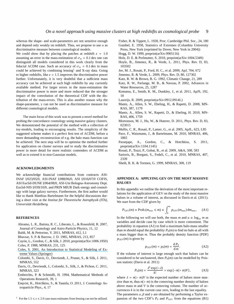
the difference between the models gets more pronounced.As mentioned above it is crucial to have the limiting mass of thesurvey in the redshift interval of interest low enough to observe thelow-mass tail of the CDF. From Fig. 10 it can be inferred that amass of roughly 1014 M⊙ h−1 would serve even in the high-redshiftcase. Due to the robustness of the cumulative measure however,also a more conservative limiting mass ofMlim ≃ 1014.5 M⊙ h−1

would still allow to recover the CDF almost equally well for the1.0 6 z 6 1.5 case as shown in Fig. 11. Such a conservative valueof Mlim will be in reach of upcoming high-redshift surveys.

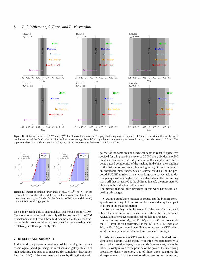
The capability to discriminate between different cosmologi-cal model of the presented method is presented in Fig. 10, wherethe difference between the valueαfit of theΛCDM and the respec-tive test-cosmologies are shown. The panels display the differenceswith an increasing mass uncertainty from left to right, where theupper row presents the results for 1.0 6 z6 1.5 case and the lowerrow for the 1.5 6 z 6 2.0 case. The grey shaded areas show multi-ples of the systematic error|αtrue− αfit | and we consider a model tobe distinguishable if its difference ofαfit is more than three timesthe systematic error. As expected, the strongest ability todistin-guish models is found for the lowest error in the mass estimatesof σm = 0.1 dex and the high-redshift case as shown in the lower-left panel of Fig. 12. Here, all test-models are significantly outsideof the grey shaded area, which they enter in the panels for biggerσm to the right. In the case ofσm = 0.2 dex the models with thestrongest difference with respect toΛCDM could still be detected.From an observational point of view the 1.0 6 z 6 1.5 case how-ever is of bigger interest since the compilation of the required sam-ple will be easier. Also for this redshift range theσm = 0.1 dex


-0.2 -0.15 -0.1 -0.05 0 0.05 0.1 0.15 0.2

∆αfit

1.0≤z≤1.5σm= 0.1 dex

INV1

SUGRA

Chaplygin

g. Chaplygin

top def w=-2/3

Phantom w=-3

ΛC

DM

-0.2 -0.15 -0.1 -0.05 0 0.05 0.1 0.15 0.2

∆αfit

1.0≤z≤1.5σm= 0.2 dex

INV1

SUGRA

Chaplygin

g. Chaplygin

top def w=-2/3

Phantom w=-3

ΛC

DM

-0.2 -0.15 -0.1 -0.05 0 0.05 0.1 0.15 0.2

∆αfit

1.0≤z≤1.5σm= 0.3 dex

INV1

SUGRA

Chaplygin

g. Chaplygin

top def w=-2/3

Phantom w=-3

ΛC

DM

-0.2 -0.15 -0.1 -0.05 0 0.05 0.1 0.15 0.2

∆αfit

1.5≤z≤2.0σm= 0.1 dex

INV1

SUGRA

Chaplygin

g. Chaplygin

top def w=-2/3

Phantom w=-3

ΛC

DM

-0.2 -0.15 -0.1 -0.05 0 0.05 0.1 0.15 0.2

∆αfit

1.5≤z≤2.0σm= 0.2 dex

INV1

SUGRA

Chaplygin

g. Chaplygin

top def w=-2/3

Phantom w=-3

ΛC

DM

-0.2 -0.15 -0.1 -0.05 0 0.05 0.1 0.15 0.2

∆αfit

1.5≤z≤2.0σm= 0.3 dex

INV1

SUGRA

Chaplygin

g. Chaplygin

top def w=-2/3

Phantom w=-3

ΛC

DM

Figure 12.Difference betweenαΛCDMfit andαmodel

fit for all considered models. The grey shaded regions correspond to 1, 2 and 3 times the difference betweenthe theoretical and the fitted value ofα for the fiducial cosmology. From left to right the mass uncertainty increases fromσm = 0.1 dex toσm = 0.3 dex. Theupper row shows the redshift interval of 1.0 6 z6 1.5 and the lower one the interval of 1.5 6 z6 2.0.

0

0.2

0.4

0.6

0.8

1

1014 1015

CD

F

mmax [MSun h-1]


α tru

e =

14.

635

α fit

= 1

4.63

47 ±

0.00

069

σm=0.1 dex

Mlim

0

0.2

0.4

0.6

0.8

1

1014 1015

CD

F

mmax [MSun h-1]


α tru

e =

14.

5511

α fit

= 1

4.53

4 ± 0

.001

12

σm=0.1 dex

Mlim

Figure 11. Impact of limiting survey mass ofMlim ≃ 1014.5 M⊙ h−1 on therecovered CDF for the 1.0 6 z 6 1.5 interval a Gaussian distributed massuncertainty withσm = 0.1 dex for the fiducialΛCDM model (left panel)and the INV1 model (right panel).

case is in principle able to distinguish all test-models fromΛCDM.The more noisy cases could probably still be used as a firstΛCDMconsistency check. Overall these findings show that the method dis-cussed in this work could be of great value for model-testingusinga relatively small sample of objects.

7 RESULTS AND SUMMARY

In this work we propose a novel method for probing our currentcosmological paradigm using the most massive galaxy clusters athigh redshifts. The idea is to measure the cumulative distributionfunction (CDF) of the most massive haloes by tiling the sky with

patches of the same area and identical depth in redshift-space. Wedecided for a hypothetical survey of 20 000 deg2, divided into 500quadratic patches of 6× 6 deg2 andδz = 0.5 sampled in 75 bins,being a good compromise of the stacking in the bins, the samplingof the distribution and sub-volumes big enough to find clusters inan observable mass range. Such a survey could e.g. be the pro-posedEUCLID mission or any other large-area survey able to de-tect galaxy clusters at high-redshifts with a sufficiently low limitingmass. All that is required is the ability to identify the mostmassiveclusters in the individual sub-volumes.The method that has been presented in this work has several ap-pealing advantages:

• Using a cumulative measure is robust and the binning corre-sponds to a stacking of clusters of similar mass, reducing the impactof errors in the mass estimation.• We are probing the high-mass tail of the mass-function, well

above the non-linear mass scale, where the difference betweenΛCDM and alternative cosmological models is strongest.• A limiting mass Mlim ≃ 1014 M⊙ h−1 is sufficient to sample

the CDF even at high redshifts. For the 1.0 6 z 6 1.5 case alsoMlim ≃ 1014.5 M⊙ h−1 would be sufficient to recover the CDF, whichwould definitely be achievable by future wide-area surveys.

In order to measure the CDF we fit a function obtained fromgeneralised extreme value theory with three free parameters γ, βandα, which are the shape-, scale- and shift-parameters, where thelatter is closely related to the position of the peak of the underlyingprobability density function. Out of these three quantities theshift-parameter,α, is the most sensitive one for model-testing,


whereas the shape- and scale-parameters are not sensitive enoughand depend only weakly on redshift. Thus, we propose to useα asdiscriminative measure between cosmological models.We could show that by placing the patches at redshiftz = 1.0assuming an error in the mass-estimation ofσm = 0.1 dex one candistinguish all models considered in this work clearly fromthefiducial ΛCDM case. Such an accuracy ofσm = 0.1 dex in masscould be achieved by combining lensing1 and X-ray data. Goingto higher redshifts, likez = 1.5 improves the discriminative powerfurther. Unfortunately, it is very doubtful that a sufficient massaccuracy can be achieved at such high redshifts by any currentlyavailable method. For larger errors in the mass-estimationthediscriminative power is more and more reduced due the strongerimpact of the convolution of the theoretical CDF with the dis-tribution of the mass-errors. This is also another reason why theshape-parameter,γ can not be used as discriminative measure fordifferent cosmological models.

The main focus of this work was to present a novel method forprobing the concordance cosmology using massive galaxy clusters.We demonstrated the potential of the method with a collection oftoy-models, leading to encouraging results. The simplicity of thesuggested scheme makes it a perfect first test ofΛCDM, before amore demanding reconstruction of e.g. the halo mass function canbe achieved. The next step will be to optimise the method furtherfor application on cluster surveys and to study the discriminativepower in more detail for more realistic contenders ofΛCDM aswell as to extend it to non-Gaussian models.

ACKNOWLEDGMENTS

We acknowledge financial contributions from contracts ASI-INAF I /023/05/0, ASI-INAF I/088/06/0, ASI I/016/07/0 COFIS,ASI Euclid-DUNE I/064/08/0, ASI-Uni Bologna-Astronomy Dept.Euclid-NIS I/039/10/0, and PRIN MIUR Dark energy and cosmol-ogy with large galaxy surveys. Furthermore, the first authorwouldlike to thank Matthias Bartelmann for the helpful discussions dur-ing a short visit at theInstitut fur Theoretische Astrophysik (ITA),Universitat Heidelberg.

REFERENCES

Abramo, L. R., Batista, R. C., Liberato, L., & Rosenfeld, R. 2007,Journal of Cosmology and Astro-Particle Physics, 11, 12

Baldi, M. & Pettorino, V. 2011, MNRAS, 412, L1Bhavsar, S. P. & Barrow, J. D. 1985, MNRAS, 213, 857Cayon, L., Gordon, C., & Silk, J. 2010, preprint(arXiv:1006.1950)Coles, P. 1988, MNRAS, 231, 125Coles, S. 2001, An Introduction to Statistical Modeling of Ex-treme Values (Springer)

Colombi, S., Davis, O., Devriendt, J., Prunet, S., & Silk, J.2011,MNRAS, 552

Davis, O., Devriendt, J., Colombi, S., Silk, J., & Pichon, C.2011,MNRAS, 323

Embrechts, P. & Schmidli, H. 1994, Mathematical Methods ofOperations Research, 39, 1

Enqvist, K., Hotchkiss, S., & Taanila, O. 2011, J. CosmologyAs-troparticle Phys., 4, 17

1 For the 1.5 6 z6 2.0 case mass estimates from lensing can not be utilised.

Fisher, R. & Tippett, L. 1928, Proc. Cambridge Phil. Soc., 24, 180Gumbel, E. 1958, Statistics of Extremes (Columbia UniversityPress, New York (reprinted by Dover, New York in 2004))

Hogg, D. W. 1999, preprint(arXiv:9905116)Holz, D. E. & Perlmutter, S. 2010, preprint(arXiv:1004.5349)Hoyle, B., Jimenez, R., & Verde, L. 2011, Phys. Rev. D, 83,103502

Jee, M. J., Rosati, P., Ford, H. C., et al. 2009, ApJ, 704, 672Jimenez, R. & Verde, L. 2009, Phys. Rev. D, 80, 127302Katz, R. W. & Brown, B. G. 1992, Climatic Change, 21, 289Katz, R. W., Parlange, M. B., & Naveau, P. 2002, Advances inWater Resources, 25, 1287

Komatsu, E., Smith, K. M., Dunkley, J., et al. 2011, ApJS, 192,18

Laureijs, R. 2009, preprint(arXiv:0912.0914L)Mantz, A., Allen, S. W., Ebeling, H., & Rapetti, D. 2008, MN-RAS, 387, 1179

Mantz, A., Allen, S. W., Rapetti, D., & Ebeling, H. 2010, MN-RAS, 406, 1759

Mortonson, M. J., Hu, W., & Huterer, D. 2011, Phys. Rev. D, 83,023015

Mullis, C. R., Rosati, P., Lamer, G., et al. 2005, ApJL, 623, L85Pace, F., Waizmann, J., & Bartelmann, M. 2010, MNRAS, 406,1865

Paranjape, A., Gordon, C., & Hotchkiss, S. 2011,preprint(arXiv:1104.1145)

Rosati, P., Tozzi, P., Gobat, R., et al. 2009, A&A, 508, 583Sartoris, B., Borgani, S., Fedeli, C., et al. 2010, MNRAS, 407,2339

Sheth, R. K. & Tormen, G. 1999, MNRAS, 308, 119

APPENDIX A: APPLYING GEV ON THE MOST MASSIVEHALOES

In this appendix we outline the derivation of the most important re-lations for the application of GEV on the study of the most massivehaloes in a volume of interest, as discussed in Davis et al. (2011).We start from the CDF given by

PGEV(m) ≡ Prob.(mmax 6 m) ≡∫ m

0pGEV(mmax) dmmax, (A1)

In the following we will use both, the massm andu ≡ log10 m asvariables and decide case by case which is more convenient. Theprobability in equation (A1) to find a maximum halo-mass smallerthanmshould equal the probabilityP0(m) to find no halo at all witha mass bigger thanm. Thus the probably density function (PDF)pGEV(m) is given by

pGEV(m) = p0(m) =d P0

dm. (A2)

If the volume of interest is large enough such that haloes canbeconsidered to be unclustered, thenP0(m) can be modelled by Pois-son statistic (Davis et al. 2011)

P0(m) =λk exp(−λ)

k!= exp [−n(> m)V] , (A3)

whereλ = n(> m)V is the expected number of haloes more mas-sive thanm, thusn(> m) is the comoving number density of haloesabove massm andV is the comoving volume. The number of oc-currencesk is in the current case zero, leading to the last equality.The parametersα, β andγ are obtained by performing a Taylor ex-pansion of the two CDF’sP0 and PGEV from the equations (B1)

http://arxiv.org/abs/1006.1950







0

0.5

1

1.5

2

2.5

3

1015

pdf (

mm

ax)

mmax [MSun h-1]

+σ-σ

E(Mmax) E(Mmax) L=100 Mpc/h GEV

Poisson

Figure A1. Probability density function of the GEV and Poisson statisticsfor a sphere of radiusL = 100 Mpch−1 at z = 0 as a function of the maxi-mum massMmax. The gray shaded area denotes the 1-σ confidence regionand the red line next to the peak (also known as mode of the distribution) isthe expected value.

and (A3) around the maxima of the distributions dP0/du andd PGEV/du, corresponding to the respective density functions. Thisgives

P0(u) = P0(u0) +d P0(u)

du

∣

∣

∣

∣

∣

u0

(u− u0) + . . . ,

PGEV(u) = PGEV(u0) +d PGEV(u)

du

∣

∣

∣

∣

∣

u0

(u− u0) + . . . ,

where theu0 = log10 m0 denotes the value ofu at which the densityfunctions have their maximum. Now, we equal the first two termsof the two expansions, the second order derivatives vanish by defi-nition and higher orders we neglect, hence one finds2

n(> m0)V =

[

1+ γ(u0 − α)β

]− 1γ

, (A4)

m0 ln 10dndm

∣

∣

∣

∣

∣

m0

V =1β

[

1+ γ(u0 − α)β

]− 1γ −1

, (A5)

where dn/dm|m0is the halo mass function evaluated atm0. To-

gether with the relation for the mode (also known as the position ofthe peak) given by

u0 = α +β

γ

[

(1+ γ)−γ − 1]

, (A6)

one arrives finally at the equations for the three parameters

γ = n(> m0)V − 1, β =(1+ γ)(1+γ)

dndm

∣

∣

∣

m0Vm0 ln 10

,

α = log10 m0 −β

γ[(1 + γ)−γ − 1] . (A7)

The most likely massm0 is obtained via the extremal condition

d2 P0

du2

∣

∣

∣

∣

∣

∣

u0

= (ln 10)2 m

(

d P0

dm+m

d2 P0

dm2

)

= 0. (A8)

which can be recast into

dndm+m

d2 ndm2

+mV

(

dndm

)2

= 0, (A9)

2 When calculating dP0/dmone should keep in mind that dn(> m)/dm=−dn/dm.

by using the definition ofP0 from equation (A3). When the massfunction of Sheth & Tormen (1999) (ST) is incorporated in theabove relation it is possible to obtain an analytic relationfor m0

(Davis et al. 2011). The ST mass function is given by

dndm=ρm

m2

d lnνd lnm

A

√

aν2π

[

1+ (aν)−p]e−aν2 , (A10)

where ρm = Ωm0ρcrit is the mean matter density today,ν =[δc/σ(m, z)]2 and the ST-parameters areA = 0.3222,a = 0.707andp = 0.3. The analytic expression form0 is then found to be

AρmVm0

√

a2πν0

e−aν0/2[

1+ (aν0)−p]

−a2−

12ν0−

ap(aν0)−(p+1)

1+ (aν0)−p+ν′′0

ν′20= 0.

(A11)

whereν0 is ν evaluated atm0 and primes denote derivatives withrespect to mass.

APPENDIX B: USEFUL RELATIONS

In this section we summarise for the reader the most important re-lations for the GEV statistic as needed for this work.

• Cumulative distribution function (CDF)

PGEV(u) = exp

−

[

1+ γ

(

u− αβ

)]−1/γ

. (B1)

• Probability density function (PDF)

pGEV(u) =1β

[

1+ γ

(

u− αβ

)]−1−1/γ

× exp

−

[

1+ γ

(

u− αβ

)]−1/γ

.

(B2)

• Mode - (most likely value)

u0 = α +β

γ

[

(1+ γ)−γ − 1]

. (B3)

• Expected value

EGEV = α −β

γ+β

γΓ (1− γ) . (B4)

• Variance

VARGEV =β2

γ2

[

Γ (1− 2γ) − Γ2 (1− γ)]

, (B5)

where Γ denotes the Gamma function. All the equations givenabove are valid forγ < 0, which is the case for the applicationsin this work.

Documents

On a novel approach using massive clusters at high redshifts as cosmological probe