On density of subgraphs of halved cubes

In memory of Michel Deza

Victor Chepoi, Arnaud Labourel, and Sebastien Ratel

Laboratoire d’Informatique Fondamentale, Aix-Marseille Universite and CNRS,Faculte des Sciences de Luminy, F-13288 Marseille Cedex 9, France

{victor.chepoi, arnaud.labourel, sebastien.ratel}@lif.univ-mrs.fr

Abstract. Let S be a family of subsets of a set X of cardinality m and VC-dim(S) be the Vapnik-Chervonenkisdimension of S. Haussler, Littlestone, and Warmuth (Inf. Comput., 1994) proved that if G1(S) = (V,E) is the

subgraph of the hypercube Qm induced by S (called the 1-inclusion graph of S), then |E||V | ≤ VC-dim(S). Haussler

(J. Combin. Th. A, 1995) presented an elegant proof of this inequality using the shifting operation.

In this note, we adapt the shifting technique to prove that if S is an arbitrary set family and G1,2(S) = (V,E)

is the 1,2-inclusion graph of S (i.e., the subgraph of the square Q2m of the hypercube Qm induced by S), then

|E||V | ≤

(d2

), where d := cVC-dim∗(S) is the clique-VC-dimension of S (which we introduce in this paper). The

1,2-inclusion graphs are exactly the subgraphs of halved cubes and comprise subgraphs of Johnson graphs as a

subclass.

1. Introduction

Let S be a family of subsets of a set X of cardinality m and VC-dim(S) be the Vapnik-Chervonenkis dimension of S. Haussler, Littlestone, and Warmuth [19, Lemma 2.4] proved thatif G1(S) = (V,E) is the subgraph of the hypercube Qm induced by S (called the 1-inclusion

graph of S), then the following fundamental inequality holds: |E||V | ≤ VC-dim(S). They used this

inequality to bound the worst-case expected risk of a prediction model of learning of conceptclasses S based on the bounded degeneracy of their 1-inclusion graphs. Haussler [18] presented anelegant proof of this inequality using the shifting (push-down) operation. 1-Inclusion graphs havemany other applications in computational learning theory, for example, in sample compressionschemes [21]. They are exactly the induced subgraphs of hypercubes and in graph theory theyhave been studied under the name of cubical graphs [14]. Finding a densest n-vertex subgraphof the hypercube Qm (i.e., an n-vertex subgraph G of Qm with the maximum number of edges)is equivalent to finding an n-vertex subgraph G of Qm with the smallest edge-boundary (thenumber of edges of Qm running between V and its complement in Qm). This is the classicaledge-isoperimetric problem for hypercubes [3,17]. Harper [16] nicely characterized the solutionsof this problem: for any n, this is the subgraph of the hypercube induced by the initial segmentof length n of the lexicographic numbering of the vertices of the hypercube. One elegant way ofproving this result is using compression [17].

Generalizing the density inequality |E||V | ≤ VC-dim(S) of [18, 19] to more general classes of

graphs is an interesting and important problem. In the current paper, we present a densityresult for 1,2-inclusion graphs G1,2(S) of arbitrary set families S. The 1,2-inclusion graphs arethe subgraphs of the square Q2

m of the hypercube Qm and they are exactly the subgraphs ofthe halved cube 1

2Qm+1. Johnson graphs and their subgraphs (for definitions, see Subsection3.2) constitute an important subclass of halved cubes. Since 1,2-inclusion graphs may containarbitrary large cliques for constant VC-dimension, we have to adapt the definition of classicalVC-dimension to capture this phenomenon. For this purpose, we introduce the notion of clique-VC-dimension cVC-dim∗(S) of any set family S. Here is the main result of the paper:

Theorem 1. Let S be an arbitrary set family of 2X with |X| = m, let d = cVC-dim∗(S) be the

clique-VC-dimension of S and G1,2(S) = (V,E) be the 1,2-inclusion graph of S. Then |E||V | ≤(d2

).

2. Related work

2.1. Haussler’s proof of the inequality |E||V | ≤ VC-dim(S). We briefly review the notion of

VC-dimension and the shifting method of [18] of proving the inequality |E||V | ≤ VC-dim(S) (the

original proof of [19] was by induction on the number of sets). In the same vein, see Harper’sproof [17, Chapter 3] of the isoperimetric inequality via compression. We will use the shiftingmethod in the proof of Theorem 1.

Let S be a family of subsets of a set X = {e1, . . . , em}; S can be viewed as a subset of verticesof the m-dimensional hypercube Qm. Denote by G1(S) the subgraph of Qm induced by thevertices of Qm corresponding to the sets of S; G1(S) is called the 1-inclusion graph of S [18,19].Vice-versa, for any subgraph G of Qm there exists a family of subsets S of 2X such that G isthe 1-inclusion graph of S. A subset Y of X is shattered by S if for all Y ′ ⊆ Y there existsS ∈ S such that S ∩ Y = Y ′. The Vapnik-Chervonenkis’s dimension [28] VC-dim(S) of S is thecardinality of the largest subset of X shattered by S.

Theorem 2 ([18, 19]). If G := G1(S) = (V,E) is the 1-inclusion graph of a set family S ⊆ 2X

with VC-dimension VC-dim(S) = d, then |E||V | ≤ d.

For a set family S ⊆ 2X , the shifting (push down or stabilization) operation ϕe with respectto an element e ∈ X replaces every set S of S such that S \ {e} /∈ S by the set S \ {e}. Denoteby ϕe(S) the resulting set family and by G′ = G1(ϕe(S)) = (V ′, E′) the 1-inclusion graph ofϕe(S). Haussler [18] proved that the shifting map ϕe has the following properties:

(1) ϕe is bijective on the vertex-sets: |V | = |V ′|,(2) ϕe is increasing in the number of edges: |E| ≤ |E′|,(3) ϕe is decreasing in the VC-dimension: VC-dim(S) ≥ VC-dim(ϕe(S)).

Harper [17, p.28] called Steiner operations the set-maps ϕ : 2X → 2X satisfying (1), (2), andthe following condition:

(4) S ⊆ T implies ϕ(S) ⊆ ϕ(T ).

He proved that the compression operation defined in [17, Subsection 3.3] is a Steiner operation.Note that ϕe satisfies (4) (but is defined only on S).

After a finite sequence of shiftings, any set family S can be transformed into a set family S∗,such that ϕe(S∗) = S∗ holds for any e ∈ X. The resulting set family S∗, a complete shiftingof S, is downward closed (i.e., is a simplicial complex). Consequently, the 1-inclusion graphG1(S∗) of S∗ is a bouquet of cubes, i.e., a union of subcubes of Qm with a common origin ∅.Let G∗ = G1(S∗) = (V ∗, E∗) and d∗ = VC-dim(S∗). Since all shiftings satisfy the conditions(1)-(3), we conclude that |V ∗| = |V |, |E∗| ≥ |E|, and d∗ ≤ d. Therefore, to prove the inequality|E||V | ≤ d it suffices to show that |E

∗||V ∗| ≤ d∗. Haussler deduced it from Sauer’s lemma [26], however

it is easy to prove this inequality directly, by bounding the degeneracy of G∗ (for the definitionof degeneracy, see Subsection 3.1). Indeed, let v0 be the vertex of G∗ corresponding to the origin∅ and let v be a furthest from v0 vertex of G∗. Then v0 and v span a maximal cube of G∗ (ofdimension ≤ d∗) and v belongs only to this maximal cube of G∗. Therefore, if we remove v fromG∗, we will also remove at most d∗ edges of G∗ and the resulting graph will be again a bouquetof cubes G− = (V −, E−) with one less vertex and dimension ≤ d∗. Therefore, we can applythe induction hypothesis to this bouquet G− and deduce that |E−| ≤ |V −|d∗. Consequently,|E∗| ≤ d∗ + |E−| ≤ d∗ + (|V ∗| − 1)d∗ = |V ∗|d∗.

2

To extend Haussler’s proof to subgraphs of halved cubes (and, equivalently, to subgraphs ofsquares of cubes), we need to appropriately define the shifting operation and the notion of VC-dimension, that satisfy the conditions (1)-(3). Additionally, the degeneracy of the 1,2-inclusiongraph of the final shifted family must be bounded by a function of the VC-dimension. We willuse the shifting operation with respect to pairs of elements (and not to single elements) and thenotion of clique-VC-dimension instead of VC-dimension.

2.2. Other results. The inequality of Haussler et al. [19] as well as the notion of VC-dimensionand Sauer lemma have been subsequently extended to subgraphs of Hamming graphs (i.e.,from binary alphabets to arbitrary alphabets); see [20, 23–25]. Cesa-Bianchi and Haussler [6]presented a graph-theoretical generalization of the Sauer lemma for the m-fold Fm = F×· · ·×FCartesian products of arbitrary undirected graphs F . In [9], we defined a notion of VC-dimensionfor subgraphs of Cartesian products of arbitrary connected graphs (hypercubes are Cartesian

products of K2) and we established a density result |E||V | ≤ VC-dim(G) · α(H) for subgraphs G

of Cartesian products of graphs not containing a fixed graph H as a minor (α(H) is a constantsuch that any graph not containing H as a minor has density at most α(H); it is well known [12]that if r := |V (H)|, then α(H) ≤ cr√log r for a universal constant c).

For edge- and vertex-isoperimetric problems in Johnson graphs (which are still open prob-lems), some authors [1,11] used a natural pushing to the left (or switching, or shifting) operation.Let S consists only of sets of size r. Given an arbitrary total order e1, . . . , em of the elementsof X and two elements ei < ej , in the pushing to the left of S with respect to the pair ei, ejeach set S of S containing ej and not containing ei is replaced by the set S \ {ej} ∪ {ei} ifS \ {ej} ∪ {ei} /∈ S. This operation preserves the size of S, the cardinality r of the sets and donot decrease the number of edges, but the degeneracy of the final graph is not easy to bound.

Bousquet and Thomasse [4] defined the notions of 2-shattering and 2VC-dimension and estab-lished the Erdos-Posa property for the families of balls of fixed radius in graphs with bounded2VC-dimension. These notions have some similarity with our concepts of c-shattering and clique-VC-dimension because they concern shattering not of all subsets but only of a certain patternof subsets (of all pairs). Recall from [4] that a set family S 2-shatters a set Y if for any 2-set{ei, ej} of Y there exists S ∈ S such that Y ∩ S = {ei, ej}; the 2VC-dimension of S is themaximum size of a 2-shattered set.

Halved cubes and Johnson graphs host several important classes of graphs occurring in metricgraph theory [2]: basis graphs of matroids are isometric subgraphs of Johnson graphs [22] andbasis graphs of even ∆-matroids are isometric subgraphs of halved cubes [7]. More generalclasses are the graphs isometrically embeddable into halved cubes and Johnson graphs. Similarlyto Djokovic’s characterization of isometric subgraphs of hypercubes [13], isometric subgraphs ofJohnson graphs have been characterized in [8] (the problem of characterizing isometric subgraphsof halved cubes has been raised in [10] and is still open). Shpectorov [27] proved that the graphsadmitting an isometric embedding into an `1-space are exactly the graphs which admit a scaleembedding into a hypercube and he proved that such graphs are exactly the graphs which areisometric subgraphs of Cartesian products of octahedra and of isometric subgraphs of halvedcubes. For a presentation of most of these results, see the book by Deza and Laurent [10].

3. Preliminaries

3.1. Degeneracy. All graphs G = (V,E) occurring in this note are finite, undirected, andsimple. The degeneracy of G is the minimal k such that there exists a total order v1, . . . , vn ofvertices of G such that each vertex vi has degree at most k in the subgraph of G induced by

3

vi, vi+1, . . . , vn. It is well known and it can be easily shown that the degeneracy of every graph

G = (V,E) upper bounds the ratio |E||V | .

3.2. Squares of hypercubes, halved cubes, and Johnson graphs. The m-dimensionalhypercube Qm is the graph having all 2m subsets of a set X = {e1, . . . , em} as the vertex-setand two sets A,B are adjacent in Qm iff |A4B| = 1. The halved cube 1

2Qm [5, 10] has the

subsets of X of even cardinality as vertices and two such vertices A,B are adjacent in 12Qm iff

|A4B| = 2 (one can also define halved cubes for subsets of odd size). Equivalently, the halvedcube 1

2Qm is the square Q2m−1 of the hypercube Qm−1, i.e., the graph formed by connecting pairs

of vertices of Qm−1 whose distance is at most two in Qm−1. For an integer r > 0, the Johnsongraph J(r,m) [5, 10] has the subsets of X of size r as vertices and two such vertices A,B areadjacent in J(r,m) iff |A4B| = 2. All Johnson graphs J(r,m) are (isometric) subgraphs of thecorresponding halved cube 1

2Qm. Notice also that the halved cube 12Qm and the Johnson graph

J(r,m) are scale 2 embedded in the hypercube Qm.Let S be a family of subsets of a set X = {e1, . . . , em}. The 1,2-inclusion graph G1,2(S) of

S is the graph having S as the vertex-set and in which two vertices A and B are adjacent iff1 ≤ |A∆B| ≤ 2, i.e., G1,2(S) is the subgraph of the square Q2

m of Qm induced by S. The graphG1,2(S) comprises all edges of the 1-inclusion graph G1(S) of S and of the subgraphs of thehalved cubes induced by even and odd sets of S. The latter edges of G1,2(S) are of two types:vertical edges SS′ arise from sets S, S′ such that |S| = |S′| + 2 or |S′| = |S| + 2 and horizontaledges SS′ arise from sets S, S′ such that |S| = |S′|.

If all sets of S have even cardinality, then we will call S an even set family; in this case, the1,2-inclusion graph G1,2(S) coincides with the subgraph of the halved cube 1

2Qm induced by S.

Since Q2m is isomorphic to 1

2Qm+1, any 1,2-inclusion graph is an induced subgraph of a halvedcube. More precisely, any set family S of X can be lifted to an even set family S+ of X∪{em+1}in such a way that the 1,2-inclusion graphs of S and S+ are isomorphic: S+ consists of all setsof even size of S and of all sets of odd size of S to which the element em+1 was added. Theproof of the following lemma is straightforward:

Lemma 1. For any set family S, the lifted family S+ is an even set family and the 1,2-inclusiongraphs G1,2(S) and G1,2(S+) are isomorphic.

3.3. Pointed set families and pointed cliques. We will call a set family S a pointed setfamily if ∅ ∈ S. Any set family S can be transformed into a pointed set family by the operationof twisting. For a set A ∈ S, let S4A := {S4A : S ∈ S} and say that S4A is obtained from Sby applying a twisting with respect to A. Note that a twisting is a bijection between S and S4Amapping the set A to ∅ (and therefore S4A is a pointed set family). Notice that any twistingof an even set family S is an even set family. As before, let G1(S) denote the 1-inclusion graphof S. The following properties of twisting are well-known and easy to prove:

Lemma 2. For any S ⊆ 2X and any A ⊆ X, G1(S4A) w G1(S) and VC-dim(S4A) =VC-dim(S).

Analogously to the proof of the first assertion of Lemma 2, one can easily show that:

Lemma 3. For any set family S ⊆ 2X and any A ⊆ X, G1,2(S4A) w G1,2(S).

We will say that a clique C of 12Qm is a pointed clique if C is a pointed set family.

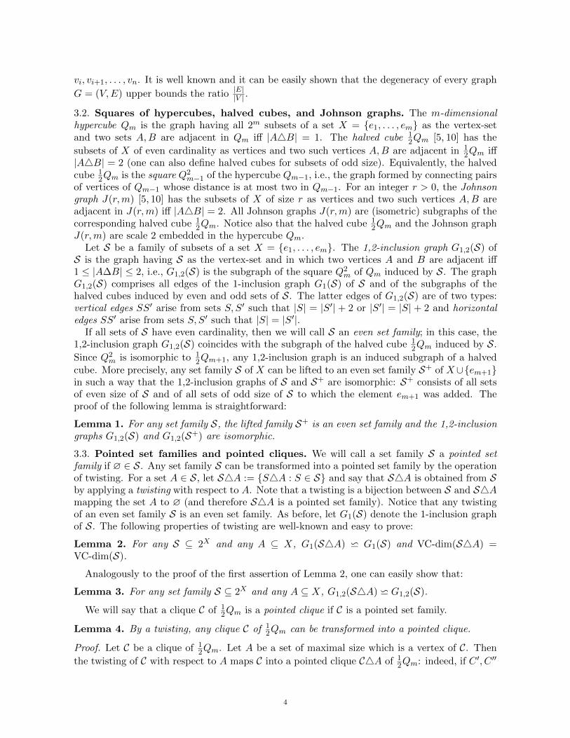
Lemma 4. By a twisting, any clique C of 12Qm can be transformed into a pointed clique.

Proof. Let C be a clique of 12Qm. Let A be a set of maximal size which is a vertex of C. Then

the twisting of C with respect to A maps C into a pointed clique C4A of 12Qm: indeed, if C ′, C ′′

4

Figure 1. A twisting mapping τ : S 7→ S4A of a clique to a pointed clique.

are two vertices of C, then |(C ′4A)4(C ′′4A)| = |C ′4C ′′| = 2. Since A∆A = ∅, C4A is apointed clique (for an illustration, see Fig. 1). �

We describe now the structure of pointed cliques in halved cubes.

Lemma 5. Any pointed maximal clique C of a halved cube 12Qm is (a) a sporadic 4-clique of the

form {∅, {ei, ej}, {ei, ek}, {ej , ek}} for arbitrary elements ei, ej , ek ∈ X, or (b) a clique of sizem of the form {∅} ∪ {{ei, ej} : ej ∈ X \ {ei}} for an arbitrary but fixed element ei ∈ X.

Proof. Since C is a pointed clique, ∅ is a vertex of C, denote it C0. All other neighbors of C0

in 12Qm are sets of the form {ei, ej} with ei, ej ∈ X, i.e., the neighborhood of C0 in the halved

cube 12Qm is the line-graph of the complete graph Km having X as the vertex-set. In particular,

the clique C0 := C \ {C0} corresponds to a set of pairwise incident edges of Km. It can be easilyseen that this set of edges defines either a triangle or a star of Km. Indeed, pick an edge eiejof Km corresponding to a pair {ei, ej} ∈ C0. If the respective set of edges is not a star, thennecessarily C0 contains two pairs of the form {ei, ek} and {ej , el}, both different from {ei, ej}.But then k = l, otherwise the edges eiek and ejel would not be incident. Thus C0 contains thethree pairs {ei, ej}, {ei, ek}, and {ej , ek}. If C0 contains yet another pair, then this pair willbe necessarily disjoint from one of the three previous pairs, a contradiction. Thus in this case,C = {∅, {ei, ej}, {ei, ek}, {ej , ek}}. Otherwise, if the respective set of edges is a star with centerei, then C0 is a clique of size m− 1 of the form {{ei, ej} : ej ∈ X \ {ei}}. �

4. The clique-VC-dimension

As we noticed above, the classical VC-dimension of set families cannot be used to boundthe density of their 1,2-inclusion graphs. Indeed, the 1,2-inclusion graph of the set familyS0 := {{ej} : ej ∈ X} is a complete graph, while the VC-dimension of S0 is 1 (notice also thatthe 2VC-dimension of S0 is 0).

We will define a notion that is more appropriate for this purpose, which we will call clique-VC-dimension. The idea is to use the form of pointed cliques of 1

2Qm established above and toshatter them. In view of Lemma 1, it suffices to define the clique-VC-dimension for even setfamilies. First we present a generalized definition of classical shattering.

Let X = {e1, . . . , em} and S ⊆ 2X . Let Y be a subset of X. Denote by Q[Y ] the subcube ofQm consisting of all subsets of Y . Analogously, for two sets Y ′ and Y such that Y ′ ⊂ Y , denoteby Q[Y ′, Y ] the smallest subcube of Qm containing the sets Y ′ and Y : Q[Y ′, Y ] = {Z ⊂ X :

5

Figure 2. Example of a c-shattered pair (ei, Y ). F (Z) is the fiber of Z inQ(ei, Y ). The sets of S (black points) in the fibers of the sets of Q(ei, Y ) areprojected on Q(ei, Y ) (in green). The vertices in Q(ei, Y ) are then mapped toP (ei, Y ) (in blue) by the c-shattering function f . The remaining vertices ofQ[∅, Y ∪ {ei}] (in red) are “not used” for shattering.

Y ′ ⊆ Z ⊆ Y }. In particular, Q[Y ] = Q[∅, Y ]. For a vertex Z of Q[Y ′, Y ], call

F (Z) := {Z ∪ Z ′ : Z ′ ⊆ X \ Y }the fiber of Z with respect to the cube Q[Y ′, Y ]. Let

πQ[Y ′,Y ](S) := {Z ∈ Q[Y ′, Y ] : F (Z) ∩ S 6= ∅}denote the projection of the set family S on Q[Y ′, Y ]. Then the cube Q[Y ′, Y ] with Y ′ ⊆ Y isshattered by S if πQ[Y ′,Y ](S) = Q[Y ′, Y ], i.e., for any Y ′ ⊆ Z ⊆ Y the fiber F (Z) contains a setof S (see Fig. 2). In particular, a subset Y is shattered by S iff πQ[Y ](S) = Q[Y ].

4.1. The clique-VC-dimension of pointed even set families. Let S be a pointed even setfamily of 2X , i.e., a set family in which all sets have even size and ∅ ∈ S. Let Y be a subset ofX and let ei be an element of X not belonging to Y . Denote by P (ei, Y ) the set of all 2-sets,i.e., pairs of the form {ei, ej} with ej ∈ Y . Then Q[{ei}, Y ∪{ei}] is the smallest subcube of Qm

containing ei and all the 2-sets of P (ei, Y ). For simplicity, we will denote this cube by Q(ei, Y ).We will say that a pair (ei, Y ) with Y ⊂ X and ei /∈ Y is c-shattered by S if there exists a

surjective function f : πQ(ei,Y )(S) → P (ei, Y ) such that for any S ∈ πQ(ei,Y )(S) the inclusionf(S) ⊆ S holds. In other words, (ei, Y ) is c-shattered by S if each 2-set {ei, ej} ∈ P (ei, Y ) admitsan extension Sj ∈ πQ(ei,Y )(S) such that {ei, ej} ⊆ Sj and for any two 2-sets {ei, ej}, {ei, ej′} ∈P (ei, Y ) the sets Sj and Sj′ are distinct. Since ∅ ∈ S, the empty set ∅ is always shattered byS.

For a pointed even set family S, the clique-VC-dimension is

cVC-dim(S) := max{|Y |+ 1 : Y ⊂ X and ∃ei ∈ X \ Y such that (ei, Y ) is c-shattered by S}.We continue with some simple examples of clique-VC-dimension:

6

Figure 3. Illustration of Example 3

Example 1. For set family S0 = {{ej} : ej ∈ X} introduced above, let S+0 = {{ej , em+1} :ej ∈ X} be the lifting of S0 to an even set family. For an arbitrary (but fixed) element ei, letS1 := {∅} ∪ {{ei, ej} : ej 6= ei}. Then S1 coincides with S0∆{ei} and with S+0 ∆{ei, em+1}. S1is an even set family, its 1,2-inclusion graph is a pointed clique, and cVC-dim(S1) = |X| = m.

Example 2. Let S2 = {∅, {e1, e2}, {e1, e3}, {e2, e3}} be the sporadic 4-clique from Lemma 5.In this case, one can c-shatter any two of the pairs {e1, e2}, {e1, e3}, {e2, e3} but not all three.This shows that cVC-dim(S2) = 2 + 1 = 3.

Example 3. For arbitrary even integers m and k, Let X be a ground set of size m+km which isthe disjoint union of m+1 sets X0, X1, . . . , Xm, where X0 = {e1, . . . , em} and Xi = {ei1, . . . , eik}for each i = 1, . . . ,m. Let S3 be the pointed even set family consisting of the empty set ∅, theset X, and for each i = 1, . . . ,m of all the 2-sets of P (ei, Xi) = {{ei, ei1}, . . . , {ei, eik}}. ThenG1,2(S3) consists of an isolated vertex X and m maximal cliques Ci := P (ei, Xi)∪{∅} of size k+1and these cliques pairwise intersect in a single vertex ∅. We assert that cVC-dim(S3) = k + 2.Indeed, let Y be the set consisting of Xi for a given i ∈ {1, . . . ,m} plus the singleton {e(i+1)1}.Then the pair (ei, Y ) is c-shattered by S3. The c-shattering map f : πQ(ei,Y )(S3) → P (ei, Y )is defined as follows: every 2-set of P (ei, Xi) ⊂ Q(ei, Y ) is in S3 and is thus mapped to itself,X ∩ (Y ∪ {ei}) = Y ∪ {ei} is an extension of the remaining 2-set {ei, e(i+1)1} in Q(ei, Y ) andthus f(Y ∪ {ei}) := {ei, e(i+1)1}. Since |Y | = k + 1, we showed that cVC-dim(S3) ≥ k + 2. Onthe other hand, cVC-dim(S3) ≤ k + 2 because every element e from X is in at most k + 1 setsof S3. Therefore, cVC-dim(S3) = k + 2.

4.2. The clique-VC-dimension of even and arbitrary set families. The clique-VC-dimension cVC-dim∗(S) of an even set family S is the minimum of the clique-VC-dimensions ofthe pointed even set families S4A for A ∈ S:

cVC-dim∗(S) := min{cVC-dim(S4A) : A ∈ S}.The clique-VC-dimension cVC-dim∗(S) of an arbitrary set family S is the clique-VC-dimensionof its lifting S+.

Remark 1. A simple analysis shows that for the even set families from Examples 1-3, we havecVC-dim∗(S1) = m, cVC-dim∗(S2) = 3, and cVC-dim∗(S3) = k + 2.

Remark 2. In fact, the set family S3 shows that the maximum degree of a 1,2-inclusion graphG1,2(S) of an even set family S can be arbitrarily larger than cVC-dim∗(S). Indeed, ∅ is thevertex of maximum degree of G1,2(S3) and its degree is km.

7

The family S3 also explains why in the definition of the clique-VC-dimension of S we takethe minimum over all S4A,A ∈ S. Consider the twisting of S3 with respect to the set X ∈S3. Then one can see that cVC-dim(S34X) ≥ (m − 1)k + 1. Indeed, S3∆X = {∅, X} ∪(⋃

(i,j)∈{1,...,m}×{1,...,k}{X\{ei, eij}}). Let Y := {eij : i ∈ {1, . . . ,m− 1} and j ∈ {1, . . . , k}}. We

assert that (e1, Y ) is c-shattered by S3∆X. We set S ′3 := πQ(e1,Y )(S3∆X), Sij := X \ {ei, eij},and S′ij := πQ(e1,Y )(Sij). Let f : S ′3 → P (e1, Y ) be such that for all i ∈ {2, . . . ,m} and j ∈{1, . . . , k}, we have f(S′ij) = {e1, e(i−1)j}. Clearly, every {e1, e(i−1)j} has an extension S′ij with a

non-empty fiber (Sij ∈ F (S′ij)), and for all Srl 6= Sij , we have S′rl 6= S′ij , hence f is a surjection.

Therefore, (e1, Y ) is c-shattered. Since |Y | = (m−1)k, whence cVC-dim(S34X) ≥ (m−1)k+1.

5. Proof of Theorem 1

After the preparatory work done in previous three subsections, here we present the proof ofour main result. We start the proof by defining the double shifting (d-shifting) as an adaptationof the shifting to pointed even families. We show that, similarly to classical shifting operation, d-shifting satisfies the conditions (1)-(3) and that the result of a complete sequence of d-shiftingsis a bouquet of halved cubes (which is a particular pointed even set family). We show that

the degeneracy of the 1,2-inclusion graph of such a bouquet B is bounded by(d2

), where d :=

cVC-dim(B). We conclude the proof of the theorem by considering arbitrary even set familiesS and applying the previous arguments to the pointed family S∆A, where A is a set of S suchthat cVC-dim(S∆A) = cVC-dim∗(S).

5.1. Double shiftings of pointed even families. For a pointed even set family S ⊆ 2X , thedouble shifting (d-shifting for short) with respect to a 2-set {ei, ej} ⊆ X is a map ϕij : S → 2X

which replaces every set S of S such that {ei, ej} ⊆ S and S \ {ei, ej} /∈ S by the set S \ {ei, ej}:ϕij : S → 2X

S 7→{S \ {ei, ej}, if {ei, ej} ⊆ S and S \ {ei, ej} /∈ SS, otherwise.

.

Proposition 1. Let S ⊆ 2X be a pointed even set family, let {ei, ej} ⊆ X be a 2-set, and letG1,2(S) = G = (V,E) and G1,2(ϕij(S)) = G′ = (V ′, E′) be the subgraphs of the halved cubeinduced by S and ϕij(S), respectively. Then |V | = |V ′| and |E| ≤ |E′| hold.

Proof. The fact that a d-shifting ϕij preserves the number of vertices of an induced subgraph ofhalved cube immediately follows from the definition. Therefore we only need to show that ϕij

cannot decrease the number of edges, i.e., that there exists an injective map ψij : E → E′. Wewill call an edge SS′ of G stable if ϕij(S) = S and ϕij(S

′) = S′ hold and shiftable otherwise.For each stable edge SS′ we will set ψij(SS

′) := SS′.Now, pick any shiftable edge SS′ of E. Notice that in this case {ei, ej} ⊆ S or {ei, ej} ⊆ S′.

To define ψij(SS′), we distinguish two cases depending on whether {ei, ej} is a subset of only

one of the sets S, S′ or of both of them.

Case 1′. {ei, ej} ⊆ S and {ei, ej} 6⊆ S′ (the case {ei, ej} ⊆ S′ and {ei, ej} 6⊆ S is similar).

Since {ei, ej} 6⊆ S′, necessarily ϕij(S′) = S′. Since SS′ is shiftable, ϕij(S) 6= S, i.e., ϕij(S) =

S \ {ei, ej} =: Z. We consider two cases depending on whether one of the elements ei or ejbelongs to S′ or not.

Subcase 1′.1. ei ∈ S′ and ej 6∈ S′ (the case ej ∈ S′ and ei 6∈ S′ is similar). In this case, thereis an element ek ∈ X such that S∆S′ = {ej , ek}. Observe that S 6⊆ S′ since ej 6∈ S′ and ej ∈ S.Hence either S′ ⊆ S or there exists A ⊂ X such that S′ = A ∪ {ek} and S = A ∪ {ej}. In the

8

former case, we have S = S′ ∪ {ej , ek}, Z = S′ ∪ {ek} \ {ei}, and Z∆S′ = {ei, ek}. In the latercase, we have Z = A \ {ei} and Z∆S′ = {ei, ek}. In both cases, |Z∆S′| = 2 and ZS′ ∈ E′. Weset ψij(SS

′) := ZS′.

Subcase 1′.2. ei 6∈ S′ and ej 6∈ S′. Then S∆S′ = {ei, ej} and so S \ {ei, ej} = Z = S′. Weobtain a contradiction that SS′ is shiftable (i.e., Z = ϕij(S) cannot be in S).

Case 2′. {ei, ej} ⊆ S and {ei, ej} ⊆ S′.Set Z := S \ {ei, ej} and Z ′ := S′ \ {ei, ej}. Then both sets Z,Z ′ belong to ϕij(S) and ZZ ′

defines an edge of G′. Since SS′ is shiftable, at least one of the sets Z,Z ′ does not belong to S.

Subcase 2′.1. Z,Z ′ /∈ S. Then ϕij(S) = Z and ϕij(S′) = Z ′ and ZZ ′ is an edge of G′. In this

case, we set ψij(SS′) := ZZ ′.

Subcase 2′.2. Z ∈ S and Z ′ /∈ S (the case Z /∈ S and Z ′ ∈ S is similar). Then ϕij(S) =S, ϕij(S

′) = Z ′, and ZZ ′ is an edge of G′ but not of G. In this case, we set ψij(SS′) := ZZ ′.

It remains to show that the map ψij : E → E′ is injective. Suppose by way of contradictionthat G′ contains an edge ZZ ′ for which there exist two distinct edges SS′ and CC ′ of G suchthat ψij(SS

′) = ψij(CC′) = ZZ ′. Since at least one of the edges SS′ and CC ′ is different from

ZZ ′, from the definition of d-shifting we conclude that ZZ ′ is not an edge of G, say Z ′ /∈ S.This also implies that SS′ and CC ′ are shiftable edges of G.

Case 1′′. Z /∈ S.

From the definition of the map ψij and since Z,Z ′ /∈ S, both edges SS′ and CC ′ are in Subcase2′.1. This shows that Z = S \ {ei, ej}, Z ′ = S′ \ {ei, ej}, and Z = C \ {ei, ej}, Z ′ = C ′ \ {ei, ej},yielding S = C and S′ = C ′, a contradiction.

Case 2′′. Z ∈ S.

After an appropriate renaming of the sets S, S′ and C,C ′, we can suppose that ϕij(S) = ϕij(C) =Z and ϕij(S

′) = ϕij(C′) = Z ′. Since Z ′ /∈ S, from the definition of the map ψij , we deduce that

S′ = Z ′ ∪ {ei, ej} = C ′. On the other hand, since Z ∈ S, we have either S = C = Z whichcontradicts the choice of SS′ 6= CC ′, or S \ {ei, ej} = C = Z (or the symmetric possibilityC \ {ei, ej} = S = Z) which contradicts the fact that SS′ (or CC ′) is shiftable.

This shows that the map ψij : E → E′ is injective, thus |E| ≤ |E′|. �

Lemma 6. If ϕij is a d-shifting of a pointed even family S ⊂ 2X , then cVC-dim(ϕij(S)) ≤cVC-dim(S).

Proof. Let (e, Y ) be c-shattered by Sij := ϕij(S) (recall that Y ⊂ X and e /∈ Y ). Let S ′ :=πQ(e,Y )(S) and S ′ij := πQ(e,Y )(ϕij(S)). By definition of c-shattering, there exists a surjective

function f associating every element of S ′ij to a 2-set {e, e′} ∈ P (e, Y ). We will define a surjective

function g from S ′ to S ′ij , and derive from f a c-shattering function f ′ := f ◦g from S ′ to P (e, Y ).

Let Se′ ∈ S ′ij be a set such that f(Se′) = {e, e′}. If Se′ ∈ S ′, then the 2-set {e, e′} also has an

extension in S ′ and we can set g(Se′) := Se′ . If Se′ 6∈ S ′, it means that there exists a set S ∈ Ssuch that S 6= ϕij(S) and ϕij(S) is in the fiber F (Se′) of Se′ with respect to πQ(e,Y ) in Sij . Theset S is in the fiber F (S′) of some set S′ ∈ S ′ with respect to πQ(e,Y ). Since ϕij(S) ⊆ S, wehave Se′ ⊆ S′ and S′ ∈ S ′ is an extension of the 2-set {e, e′}. We set g(S′) := Se′ . Moreover, forevery set S′ ∈ S ′ \ S ′ij , there is a set S ∈ F (S′) such that ϕij(S) 6= S. In this case, there is a set

Se′ ∈ S ′ij such that ϕij(S) ∈ F (Se′). We set g(S′) := Se′ . We have Se′ ⊆ S′ since ϕij(S) ⊂ S.

The function g is surjective by definition and maps every set of S ′ either on itself or on asubset of it. Since f is a c-shattering function, so is f ′ := f ◦ g and (e, Y ) is c-shattered by S.

9

f

f ′ = f ◦ g

g

Q(e, Y )

F (Se′)F (S′)

∅ Y ∪ {e}Se′

ϕij(S)

{e}{e, e′}

S′

S

Figure 4. To the proof of Lemma 6.

Consequently, we have cVC-dim(ϕij(S)) ≤ cVC-dim(S) since every (e, Y ) c-shattered by Sij isalso c-shattered by S. �

5.2. Bouquets of halved cubes. A bouquet of cubes (called usually a downward closed familyor a simplicial complex) is a set family B ⊆ 2X such that S ∈ B and S′ ⊆ S implies S′ ∈ B.Obviously B is a pointed family. Note that any bouquet of cubes B is the union of all cubes ofthe form Q[∅, S], where S is an inclusion-wise maximal subset of B.

A bouquet of halved cubes is an even set family B ⊆ 2X such that for any S ∈ B, any subsetS′ of S of even size is included in B. In other words, a bouquet of halved cubes B is the unionof all halved cubes spanned by ∅ and inclusion-wise maximal subsets S of B.

Lemma 7. After a finite number of d-shiftings, any pointed even set family S of 2X can betransformed into a bouquet of halved cubes.

Proof. Let S0,S1,S2, . . . be a sequence of even set families such that S0 = S and, for any i ≥ 1,Si was obtained from Si−1 by a d-shifting and Si 6= Si−1. This sequence is necessarily finitebecause each d-shifting strictly decreases the sum of sizes of the sets in the family. Let Sr denotethe last family in the sequence. This means that the d-shifting of Sr with respect to any pair ofelements of X leads to the same set family Sr. Therefore, for any set S ∈ Sr and for any pair{ej , ek} ⊆ S, the set S \ {ej , ek} belongs to Sr, i.e., Sr is a bouquet of halved cubes. �

We continue with simple properties of bouquets of halved cubes.

Lemma 8. Let B ⊂ 2X be a bouquet of halved cubes of clique-VC-dimension d := cVC-dim(B).Then the following properties hold:

(i) for any element ei ∈ X, |{{ei, ej} ∈ B : ej ∈ X \ {ei}}| ≤ d− 1;(ii) if S is a set of B, then |S| ≤ d;(iii) if S is a set of B maximal by inclusion, then B \ {S} is still a bouquet of halved cubes.

Proof. The inequality |{{ei, ej} ∈ S : ej ∈ X \ {ei}}| ≤ d− 1 directly follows from the definitionof cVC-dim(B). The property (iii) immediately follows from the definition of a bouquet of halvedcubes. To prove (ii), suppose by way of contradiction that |S| > d. Since B is a bouquet ofhalved cubes, every subset of S of even cardinality belongs to B. Therefore, if we pick any e ∈ Sand if we set Y := S \ {e}, then all the 2-sets of the form {e, e′} with e′ ∈ Y are subsets of S,

10

and thus are sets of B. Consequently (e, Y ) is c-shattered by B. Since |Y | = |S| − 1 > d − 1,this contradicts the assumption that d = cVC-dim(B). �

5.3. Degeneracy of bouquets of halved cubes. In this subsection we prove the followingupper bound for degeneracy of 1,2-inclusion graphs of bouquets of halved cubes:

Proposition 2. Let B ⊂ 2X be a bouquet of halved cubes of clique-VC-dimension d :=cVC-dim(B), and let G := G1,2(B). Then the degeneracy of G is at most

(d2

).

Proof. Let S be a set of maximal size of B. By Lemma 8(iii), B \ {S} is a bouquet of halved

cubes. Thus, it suffices to show that the degree of S in G is upper bounded by(d2

). From Lemma

8(ii), we know that |S| ≤ d. This implies that S is incident in G to at most(d2

)vertical edges.

Therefore, it remains to bound the number of horizontal edges sharing S. The following lemmawill be useful for this purpose:

Lemma 9. If |S| = d− k ≤ d, then S is incident in G to at most (d− k)k horizontal edges.

Proof. Pick any s ∈ S and set Y := S \ {s}. For an element e ∈ X \ S, let Ses := Y ∪ {e}.

Notice that such Ses are exactly the neighbors of S in 1

2Qm connected by a horizontal edge. LetX ′ = {e ∈ X \ S : Se

s ∈ B}.Pick any element y ∈ Y . Then y ∈ Se

s for any e ∈ X ′. Since B is a bouquet of halved cubes,each of the d − k − 1 pairs {y, e′} with e′ ∈ S \ {y} belongs to B (yielding P (y, S \ {y}) ⊆ B).To each set Se

s , e ∈ X ′, corresponds the unique pair {y, e} and {y, e} ∈ B because y, e ∈ Ses .

Therefore P (y,X ′) ⊂ B. Since |P (y, S \ {y})| + |P (y,X ′)| ≤ d − 1 and |P (y, S \ {y})| =d− k − 1, |X ′| = |P (y,X ′)|, we conclude that |X ′| ≤ k. Therefore, for a fixed element s ∈ S, Shas at most k neighbors of the form Se

s with e ∈ X ′. Since there are |S| = d− k possible choicesof the element s, S has at most (d− k)k neighbors of cardinality |S|. �

We now continue the proof of Proposition 2. Let |S| = d − k ≤ d. Then S has(d−k2

)neighbors of the form S\{e, e′} with e 6= e′ ∈ S, i.e., S has

(d−k2

)incident vertical edges. It

remains to bound the number of neighbors of S of the form S\{e} ∪ {e′} with e ∈ S ande′ ∈ X \ S. By Lemma 9, S has at most (d − k)k such neighbors. Summarizing, S possesses

(d − k)k +(d−k2

)= 1

2(d2 − d − k2 + k) neighbors in G, and this number is maximal for k = 0because

1

2(d2 − d− k2 + k) =

1

2(d2 − d)− 1

2(k2 − k) =

(d

2

)−(k

2

)≤(d

2

).

Hence, the degree of S in G is at most(d2

), as asserted. �

5.4. Proof of Theorem 1. First, let S be an even set family over X with |X| = m, d =cVC-dim∗(S) be the clique-VC-dimension of S, and G1,2(S) = (V,E) be the 1,2-inclusion graph

of S. We have to prove that |E||V | ≤(d2

)=: D.

Let A be a set of S such that cVC-dim(S∆A) = cVC-dim∗(S) = d. By Lemma 3,

G1,2(S4A) w G1,2(S). Thus it suffices to prove the inequality|E(G1,2(S4A))||V (G1,2(S4A))| ≤ D. Consider

a complete sequence of d-shiftings of S4A and denote by (S4A)∗ the resulting set family.Since S4A is a pointed even set family, applying Lemma 6 to each d-shifting, we deduce thatcVC-dim((S4A)∗) ≤ cVC-dim(S4A) = d. By Lemma 7, (S4A)∗ is a bouquet of halved cubes,thus, by Proposition 2, the degeneracy of its 1,2-inclusion graph G∗ = G1,2((S4A)∗) is at most

D. Therefore, if G∗ = (V ∗, E∗), then |E∗|

|V ∗| ≤ D (here we used the fact that the degeneracy of a

graph G = (V,E) is an upper bound for the ratio |E||V |). Applying Proposition 1 to each of the

d-shiftings and taking into account that G1,2(S4A) w G1,2(S), we conclude that |E||V | ≤|E∗||V ∗| ,

11

yielding the required density inequality |E||V | ≤ D and finishing the proof of Theorem 1 in case

of even set families. If S is an arbitrary set family, then cVC-dim∗(S) = cVC-dim∗(S+), whereS+ is the lifting of S to an even set family. Since by Lemma 1, S and S+ have isomorphic 1,2-inclusion graphs, the density result for S follows from the density result for S+. This concludesthe proof of Theorem 1.

Example 4. As in the case of classical VC-dimension and Theorem 2, the inequality fromTheorem 1 between the density of 1,2-inclusion graph G1,2(S) and the clique-VC-dimension ofS is sharp in the following sense: there exist even set families S such that the degeneracy ofG1,2(S) equals to

(d2

). For example, the sporadic clique S2 has clique VC-dimension 3 (see

Examples 2 and remark 1), degeneracy 3, and density 32). Notice that G1,2(S2) is the halved

cube 12Q3. More generally, let S4 be the even set family consisting of all even subsets of an

m-set X. Clearly d := cVC-dim∗(S4) = |X| = m and S4 induces the halved cube 12Qm. We

assert that 12Qm has degeneracy

(d2

). Indeed, every S ∈ S4 is incident to

(|X|−|S|2

)supersets of

cardinality |S|+ 2, to(|S|

2

)subsets of cardinality |S| − 2, and to |S|(|X| − |S|) sets of cardinality

|S|. Setting s := |S|, we conclude that each set S has degree

(m− s)(m− s− 1) + s(s− 1)

2+ s(m− s) =

1

2(m2 −m) =

1

2(d2 − d) =

(d

2

).

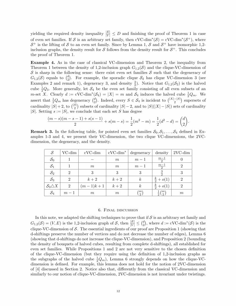
Remark 3. In the following table, for pointed even set families S0,S1, . . . ,S4 defined in Ex-amples 1-3 and 4, we present their VC-dimension, the two clique VC-dimensions, the 2VC-dimension, the degeneracy, and the density.

S VC-dim cVC-dim cVC-dim∗ degeneracy density 2VC-dim

S0 1 − m m− 1 m−12 0

S1 1 m m m− 1 m−12 2

S2 2 3 3 3 32 3

S3 2 k + 2 k + 2 k k2 + o(1) 2

S34X 2 (m− 1)k + 1 k + 2 k k2 + o(1) 2

S4 m− 1 m m(m2

)12

(m2

)m

6. Final discussion

In this note, we adapted the shifting techniques to prove that if S is an arbitrary set family and

G1,2(S) = (V,E) is the 1,2-inclusion graph of S, then |E||V | ≤(d2

), where d := cVC-dim∗(S) is the

clique-VC-dimension of S. The essential ingredients of our proof are Proposition 1 (showing thatd-shiftings preserve the number of vertices and do not decrease the number of edges), Lemma 6(showing that d-shiftings do not increase the clique-VC-dimension), and Proposition 2 (boundingthe density of bouquets of halved cubes, resulting from complete d-shiftings), all established foreven set families. While Propositions 1 and 2 are not very sensitive to the chosen definitionof the clique-VC-dimension (but they require using the definition of 1,2-inclusion graphs asthe subgraphs of the halved cube 1

2Qm), Lemma 6 strongly depends on how the clique-VC-dimension is defined. For example, this lemma does not hold for the notion of 2VC-dimensionof [4] discussed in Section 2. Notice also that, differently from the classical VC-dimension andsimilarly to our notion of clique-VC-dimension, 2VC-dimension is not invariant under twistings.

12

In analogy to 2-shattering and 2VC-dimension, we can define the concepts of star-shatteringand star-VC-dimension, which might be useful for finding sharper upper bounds (than thoseobtained in this paper) for density of 1,2-inclusion graphs. Let Y ⊂ X and e /∈ Y . We say thata set family S star-shatters (or s-shatters) the pair (e, Y ) if for any y ∈ Y there exists a setS ∈ S such that S ∩ (Y ∪ {e}) = {e, y}. The star-VC-dimension of a pointed set family S is

sVC-dim(S) := max{|Y |+ 1 : Y ⊂ X and ∃ei ∈ X \ Y such that (ei, Y ) is s-shattered by S}.The difference with c-shattering is that, in the definition of s-shattering, a pair (e, Y ) is s-shattered if all 2-sets of P (e, Y ) have non-empty fibers, i.e., if P (e, Y ) ⊆ πQ(e,Y )(S). Con-sequently, any s-shattered pair (e, Y ) is c-shattered, thus sVC-dim(S) ≤ cVC-dim(S). SincesVC-dim(S34X) = 3 and G1,2(S34X) contains a clique of size k + 1, sVC-dim(S) cannot beused directly to bound the density of 1,2-inclusion graphs. We can adapt this notion by takingthe maximum over all twistings with respect to sets of S: the star-VC-dimension sVC-dim∗(S) ofan arbitrary set family S is max{sVC-dim(S∆A) : A ∈ S}1. Even if sVC-dim(S) ≤ cVC-dim(S)holds for pointed families, as the following examples show, there are no relationships betweencVC-dim∗(S) and sVC-dim∗(S) for even families.

Example 5. Let X = {1, 2, . . . , 2m − 1, 2m}, where m is an arbitrary even integer, and letS5 := {∅} ∪ {{1, 2, . . . , 2i − 1, 2i} : i = 1, . . . ,m}. The nonempty sets of S5 can be viewed asintervals of even length of N with a common origin. The 1,2-inclusion graph of S5 is a path oflength m. For any set {1, 2, . . . , 2i}, the twisted family Si5 := S54{1, 2, . . . , 2i} is the union ofthe set families S ′ := {∅, {2i+ 1, 2i+ 2}, . . . , {2i+ 1, 2i+ 2, . . . , 2m}} and S ′′ := {{1, 2, . . . , 2i−1, 2i}, . . . , {2i − 1, 2i}}. We assert that for any i = 1, . . . ,m, we have sVC-dim(Si5) ≤ 3 andcVC-dim(Si5) = max{i,m− i}+ 1. Indeed, for any element j ∈ X, Si5 cannot simultaneously s-shatter two pairs {j, l1}, {j, l2} with j < l1 < l2 because every set of Si5 containing l2 also containsl1. Analogously, Si5 cannot s-shatter two pairs {j, l1} and {j, l2} with l2 < l1 < j. Consequently,if the pair (j, Y ) is s-shattered by Si5, then |Y | ≤ 2. This shows that sVC-dim∗(S5) ≤ 3.

To see that cVC-dim(Si5) = max{i,m−i}+1, notice that S ′ c-shatters the pair (2i+1, Y ′) withY ′ := {2i + 2, 2i + 4, . . . , 2m} and S ′′ c-shatters the pair (2i, Y ′′) with Y ′′ := {1, 3, . . . , 2i− 1}.Since the minimum over all i = 1, . . . ,m of max{i,m − i} + 1 is attained for i = m

2 , weconclude that cVC-dim∗(S5) = m

2 + 1. Therefore sVC-dim∗(S) can be arbitrarily smaller thancVC-dim∗(S).

Example 6. Let X = X1∪X2 with X1 = {e1, . . . , em} and X2 = {x1, . . . , xm}, and let S6 :={∅, {e1, x1}} ∪ {{e1, ei, x1, xi} : 2 ≤ i ≤ m}. The 1,2-inclusion graph of S6 is a star. One caneasily see that sVC-dim(S6) = m. On the other hand, for the twisted family S ′6 := S64{e1, x1} ={∅}∪{{ei, xi} : 1 ≤ i ≤ m}, one can check that cVC-dim(S ′6) = 2, showing that cVC-dim∗(S6) =2 and sVC-dim∗(S6) = m. Therefore sVC-dim∗(S) can be arbitrarily larger than cVC-dim∗(S).

Therefore, it is natural to ask whether in Theorem 1 one can replace cVC-dim∗(S) bysVC-dim∗(S). However, we were not able to decide the status of the following question:

Question 1. Is it true that for any (even) set family S with the 1,2-inclusion graph G1,2(S) =

(V,E) and star-VC-dimension d = sVC-dim∗(S), we have |E||V | = O(d2)?

The main difficulty here is that a d-shifting may increase the star-VC-dimension, i.e., Lemma6 does no longer hold. The difference between the s-shattering and c-shattering is that a 2-set{e, y} with y ∈ Y can be s-shattered only by a set S ∈ S which belongs to the fiber F ({e, y})(the requirement Y ∩ S = {e, y}), while {e, y} can be c-shattered by a set S if S just includes

1As noticed by one referee and O. Bousquet, in this form, the star-VC-dimension minus one coincides with thenotion of star number that has been studied in the context of active learning [15, Definition 2].

13

this set (the requirement {e, y} ⊆ S). When performing a d-shifting ϕij with respect to a pair{ei, ej} such that {ei, ej} ∩ {e, y} = ∅, a set S ∈ S can be mapped to a set ϕij(S) belonging tothe fiber F ({e, y}). If ϕij(S) is used to c-shatter the 2-set {e, y} by ϕij(S), then S can be usedto shatter {e, y} by S (the proof of Lemma 6). However, this is no longer true for s-shattering,because initially S may not necessarily belong to F ({e, y}).

Also we have not found a counterexample to the following question (where the square of theclique-VC-dimension or of the star-VC-dimension is replaced by the product of the classicalVC-dimension of S and the clique number of G1,2(S)):

Question 2. Is it true that for any set family S with 1,2-inclusion graph G1,2(S) = (V,E),

d = VC-dim(S), and clique number ω = ω(G1,2(S)), we have |E||V | = O(d · ω)?

Hypercubes are subgraphs of Johnson graphs, therefore they are 1,2-inclusion graphs. Thisshows the necessity of both parameters (VC-dimension and clique number) in the formulationof Question 2. As above, the bottleneck in solving Question 2 via shifting is that this operationmay increase the clique number of 1,2-inclusion graphs.

An alternative approach to Questions 1 and 2 is to adapt the original proof of Theorem 2 givenin [19]. In brief, for a set family S of VC-dimension d and an element e, let Se = {S′ ⊆ X \{e} :S′ = S ∩ X for some S ∈ S} and Se = {S′ ⊆ X \ {e} : S′ and S′ ∪ {e} belong to S}. Then|S| = |Se|+ |Se|, VC-dim(Se) ≤ d, and VC-dim(Se) ≤ d− 1 hold. Denote by Ge and Ge the 1-inclusion graphs of Se and Se. Then |E(Ge)| ≤ d|V (Ge)| = d|Se| and E(Ge) ≤ (d− 1)|V (Ge)| =(d − 1)|Se| by induction hypothesis. The proof of the required density inequality follows byinduction from the equality |V (G)| = |S| = |Se| + |Se| = |V (Ge)| + |V (Ge)| and the inequality|E(G)| ≤ |E(Ge)| + |E(Ge)| + |V (Ge)|. Unfortunately, as was the case for shiftings, the cliquenumber of G1,2(Se) may be strictly larger than the clique number of G1,2(S). Also the inequality|E(G)| ≤ |E(Ge)| + |E(Ge)| + |V (Ge)| is no longer true in this form if instead of 1-inclusiongraphs one consider 1,2-inclusion graphs.

Acknowledgements. We would like to acknowledge the anonymous referees for a carefulreading of the previous version and many useful remarks. We are especially indebted to one ofthe referees who found a critical error in the previous proof of Proposition 1. We would like toacknowledge another referee and Olivier Bousquet for pointing to us the paper [15]. This workwas supported in part by ANR project DISTANCIA (ANR-17-CE40-0015).

References

[1] R. Ahlswede and N. Cai, A counterexample to Kleitman’s conjecture concerning an edge-isoperimetric prob-lem, Combinatorics, Probability and Computing 8 (1999), 301–305.

[2] H.-J. Bandelt and V. Chepoi, Metric graph theory and geometry: a survey, in: J. E. Goodman, J. Pach, R.Pollack (Eds.), Surveys on Discrete and Computational Geometry. Twenty Years later, Contemp. Math., vol.453, AMS, Providence, RI, 2008, pp. 49–86.

[3] S. L Bezrukov, Edge isoperimetric problems on graphs, Proc. Bolyai Math. Studies 449 (1998).[4] N. Bousquet and S. Thomasse, VC-dimension and Erdos-Posa property, Discr. Math. 338 (2015), 2302–2317.[5] A.E. Brouwer, A.M. Cohen, and A. Neumaier, Distance Regular Graphs, Springer-Verlag Berlin, New York,

1989.[6] N. Cesa-Bianchi and D. Haussler, A graph-theoretic generalization of Sauer-Shelah lemma, Discr. Appl.

Math. 86 (1998), 27–35.[7] V. Chepoi, Basis graphs of even Delta-matroids, J. Combin. Th. Ser B 97 (2007), 175–192.[8] V. Chepoi, Distance-preserving subgraphs of Johnson graphs, Combinatorica (to appear).[9] V. Chepoi, A. Labourel, and S. Ratel, On density of subgraphs of Cartesian products, (in preparation).

[10] M. Deza and M. Laurent, Geometry of Cuts and Metrics, Springer-Verlag, Berlin, 1997.[11] V. Diego, O. Serra, and L. Vena, On a problem by Shapozenko on Johnson graphs, arXiv:1604.05084, 2016.[12] R. Diestel, Graph Theory, Graduate texts in mathematics, Springer New York, Berlin, Paris, 1997.[13] D.Z. Djokovic, Distance–preserving subgraphs of hypercubes, J. Combin. Th. Ser. B 14 (1973), 263–267.

14

[14] M.R. Garey and R.L. Graham, On cubical graphs, J. Combin. Th. B 18 (1975), 84–95.[15] S. Hanneke and L. Yang, Minimax analysis of active learning, J. Mach. Learn. Res. 16 (2015), 3487–3602.[16] L.H. Harper, Optimal assignments of numbers to vertices, SIAM J. Appl. Math., 12 (1964), 131–135.[17] L.H. Harper, Global Methods for Combinatorial Isoperimetric Problems, Cambridge Studies in Advanced

Mathematics (No. 90), Cambridge University Press 2004.[18] D. Haussler, Sphere packing numbers for subsets of the Boolean n-cube with bounded Vapnik-Chervonenkis

dimension, J. Comb. Th. Ser. A 69 (1995), 217–232.[19] D. Haussler, N. Littlestone, and M. K. Warmuth, Predicting {0, 1}-functions on randomly drawn points, Inf.

Comput. 115 (1994), 248–292.[20] D. Haussler and P.M. Long, A generalization of Sauer’s lemma. J. Combin. Th. Ser. A 71 (1995), 219–240.[21] D. Kuzmin and M.K. Warmuth, Unlabelled compression schemes for maximum classes, J. Mach. Learn. Res.

8 (2007), 2047–2081.[22] S.B. Maurer, Matroid basis graphs I, J. Combin. Th. Ser. B 14 (1973), 216–240.[23] B. K. Natarajan, On learning sets and functions, Machine Learning 4 (1989), 67–97.[24] D. Pollard, Convergence of Stochastic Processes, Springer Science & Business Media, 2012.[25] B.I. Rubinstein, P.L. Bartlett, and J.H. Rubinstein, Shifting: one-inclusion mistake bounds and sample

compression, J. Comput. Syst. Sci. 75 (2009), 37–59.[26] N. Sauer, On the density of families of sets, J. Combin. Th., Ser. A 13 (1972), 145–147.[27] S.V. Shpectorov, On scale embeddings of graphs into hypercubes, Europ. J. Combin. 14 (1993), 117–130.[28] V.N. Vapnik and A.Y. Chervonenkis, On the uniform convergence of relative frequencies of events to their

probabilities, Theory Probab. Appl. 16 (1971), 264–280.

15