On Hunger and Child Mortality in India

Economics Discussion Paper Series EDP-0907

On hunger and child mortality in India

Raghav Gaiha Vani Kulkarni Manoj Pandey Katsushi Imai

May 2009

Economics School of Social Sciences

The University of Manchester Manchester M13 9PL

On Hunger and Child Mortality in India1*

Raghav Gaiha

Centre for Population and Development Studies, Harvard University, MA, USA and Faculty of Management Studies, University of Delhi. India

Vani S. Kulkarni

Department of Sociology, Harvard University, MA, USA

Manoj K. Pandey Institute of Economic Growth, Delhi, India

Katsushi S. Imai2

Economics, School of Social Sciences, University of Manchester, UK

7th May 2009

Abstract

Despite accelerated growth there is pervasive hunger, child undernutrition and mortality. Our analysis focuses on their determinants. Raising living standards alone will not reduce hunger and undernutrition. Reduction of rural/urban disparities, income inequality, consumer price stabilisation, and mothers’ literacy have all roles of varying importance in different nutrition indicators. Somewhat surprisingly, PDS (Public Distribution Systems) does not have a significant effect on any of them. Generally, child undernutrition and mortality rise with poverty. Our analysis confirms that media exposure triggers public action, and helps avert child undernutrition and mortality. Drastic reduction of economic inequality is in fact key to averting child mortality.

Keywords: Hunger, underweight, child mortality, prices, inequality, literacy, India

JEL Codes: I10, I31, I32

1 We are grateful to Raghbendra Jha and Varsha S. Kulkarni for useful discussions. The views expressed are, however, personal and not necessarily of the institutions to which they are affiliated. 2 Corresponding Author: Dr Katsushi S. Imai, Economics, School of Social Sciences, University of Manchester, Arthur Lewis Building, Oxford Road, Manchester M13 9PL, UK; Telephone: +44-(0)161-275-4827, Fax: +44-(0)161-275-4812 Email: [email protected].

2

On Hunger and Child Mortality in India

I. Introduction

India has recorded an unprecedented growth in recent years-in fact; it is regarded as one of the

fastest growing economies in the world. Real gross domestic product (GDP) per capita grew at

3.95 per cent annually during 1980-2005, and at 5.4 per cent annually from 2000 to 2005. Real

per capita consumption growth also accelerated-from 2.2 per cent a year in the 1980s, at 2.5 per

cent a year in the 1990s, and at 3.9 per cent a year from 2000 to 2005. Although household

surveys register slower growth rates of consumption, there has been a significant reduction in

poverty since the early 1980s (Deaton and Dreze, 2002, Jha et al., 2009 a, and Himanshu, 2007,

Gaiha et al. 2008). Yet per capita calorie intake has declined, as also of many other nutrients. In

fact, as noted in Deaton and Dreze, 2008, more than three quarters of the population live in

households whose per capita calorie intake is less than 2,100 in urban areas and 2400 in rural

areas-calorie intakes regarded as “minimum requirements’ in India3. A related concern is that

anthropometric indicators tell an equally dismal story. Some of these indicators are the worst in

the world. Besides, improvements in these indicators are sluggish despite impressive economic

growth. Indeed, according to the National Family Health Survey (NFHS hereafter), the

proportion of underweight children remained virtually unchanged between 1998-99 and 2005-

06-from 47 to 46 per cent for the age-group 0-3 years (Deaton and Dreze, 2008)4.

3 Deaton and Dreze, 2008, draw attention to a downward shift of the ‘calorie Engel curve” that plots calorie consumption against per capita household expenditure: calorie consumption at a given level of per capita expenditure has steadily declined over the last 20 years. Why this should happen in a country as poor and malnourished as India is intriguing. For a conjecture, see Deaton and Dreze, 2008. 4 Deaton and Dreze, 2008, are emphatic “ Undernutrition levels in India remain higher even than for most countries of Sub-Saharan Africa, even though those countries are much poorer than India, have grown much more slowly, and have much higher levels of infant and child mortality”, (p.2).

3

A fascinating new study (Menon et al. 2009) draws an equally gloomy picture. Although serious

doubts remain about the appropriateness of the Global Hunger Index (GHI) constructed by the

International Food Policy Research Institute (IFPRI) researchers (e.g. aggregation of three

indicators -inadequate consumption, child underweight, and child mortality is deeply

problematic), its application to 17 major Indian states is of considerable interest5. This analysis is

based on the third round of the NFHS (2005-06) -hereafter referred to as NFHS-III data- and the

61st round of the NSS data for 2004-05.

Contrary to the views of the authors, the severity of hunger is better reflected in the individual

components than in the State Hunger Index. Using the calorie undernutrition measure based on a

calorie cut-off of 1632 kcals per person per day, the average works out to be 20 per cent6, 7. At

least, three states were well above the average (viz. Tamil Nadu (29.1 per cent), Kerala (28.6 per

cent), and Karnataka (28.1 per cent). The second component-proportion of underweight children

under 5 years- was estimated at the state level using data from the NFHS-III data. This denotes

the proportion of children in each state whose weight-for-age was less than two standard

deviations below the WHO reference. The average for all-India is 42.5 per cent8. Bihar (56.1 per

cent), Jharkand (57.1 per cent) and Madhya Pradesh (59.8 per cent) were among the worst

performers. The third indicator, under-five mortality rate (deaths per hundred), averaged 7.4,

5 As noted by Menon et al. 2009, the GHI 2008 reveals India’s continued lacklustre performance at eradicating hunger: India ranks 66th out of the 88 developing countries and countries in transition for which the index has been calculated. 6 Note that typically higher calorie norms are used in the Indian context. Deaton and Dreze, 2008, for example, report that the share of population consuming less than 2400 kcals per day was 66.1 per cent in rural India in 2004-05, and the share consuming less than 2100 kcals per day in urban India was nearly 61 per cent. The all-India average was thus as high as nearly 65 per cent of the population. That is, three times higher than that reported by Menon et al., 2009. 7 In important contributions, Srinivasan ,1981, 1992, 1994, argues cogently against the usefulness of calorie norms. This concern is echoed by Deaton and Dreze, 2008. They emphasise that there are too many sources of variation in calorie-requirements for standard, time-invariant calorie norms to be usefully applied to large segments of the population. 8 Deaton and Dreze, 2008, report the proportions of underweight children below three standard deviations of the WHO reference: these were 17.6 per cent in 1998-99 and 15.8 per cent in 2005-06. The stunting estimates were high too and recorded a slight reduction over this period: from 51 per cent to 44.9 per cent.

4

with Uttar Pradesh (9.6), Jharkand (9.3) and Madhya Pradesh (9.4) among those with the most

dismal performance9.

The objective of the present study is to build on these important contributions, by estimating in

greater detail the underlying determinants of hunger, child undernutrition, and mortality. Using

the state-level data based on recent rounds of national household survey data in India, namely

NSS and NFHS, it is hoped, some new light will be thrown on policy priorities. The rest of the

paper is structured as follows. Section II briefly describes the data. In Section III, we discuss the

specifications for each nutritional indicator, followed by a discussion of the results in Section IV.

Finally, Section V assesses these findings from a broad policy perspective.

II. Data

This study draws upon 61st round of nationwide household consumer expenditure survey data

conducted by National Sample Survey Organisation (NSSO) in 2004-05 and latest National

Family Health Survey (NFHS) Data-III in 2005-06. The NSSO, set up by the Government of

India in 1950, is a multi-subject integrated sample survey conducted at all-India level in the form

of successive rounds relating to various aspects of social, economic, demographic, industrial and

agricultural statistics.10 Mainly we use consumer expenditure data as well as variables on child

mortality from NSSO datasets. Similarly, NFHS is another major nationwide, large multi-round

survey conducted in a representative sample of households in India with a focus on health and

9 Deaton and Dreze, 2008, explore combining intake data with outcome focused indicators, such as anthropometric indicators. However, anthropometric measures have their own limitations. First, there are unresolved puzzles, such as high prevalence of stunting among affluent children. Secondly, there are inconsistencies between different sources of data (viz. National Family Health Survey and National Nutrition Monitoring Bureau). While broad long-term trends are reasonably clear, there is some inconsistency about recent changes (p.10). 10 See the website of National Sample Survey Organisation http://mospi.nic.in/nsso_test1.htm for more details of NSS.

5

nutrition of household members, especially of women and young children. The data include the

variables on calorie under-nourishment or underweight children and or mortality rates of children

under five years.11 Because of lack of consistent district code in NFHS, only feasible way of

estimating the determinants of child undernutrition is to aggregate the data at the state level, as

done by Menon et al. 2009. Apart from these variables, we also have borrowed education for

women (e.g. female literacy rate) of age-group 15-49. While the results will have to be

interpreted with caution because the aggregation bias arising from the omission of variation

within state, the analysis of determinants of undernutrition is worthwhile as it may yield useful

policy insights. Some of the variables of interests also have been drawn from other published

articles including those from various economic and political weekly (EPW) issues.

II. Specification

Let us first consider the determinants of calorie intake. Algebraically, prevalence of calorie-

undernourishment is posited to depend on

)1.....(......................................................................

)()()(

165

243

2210

ii

iiiii

BIMARUMPCEUrbantoRatioRural

CPIALCPIALMPCEMPCEtNourishmenUnderCalorieLog

εβββββββ

+++++++=

where the right-hand side variables are monthly per capita expenditure (MPCE), its square,

Consumer Price Index for Agricultural Labourers (CPIAL), its square, ratio of rural MPCE to

urban MPCE, and whether a state belonged to the BIMARU group of states (Bihar, Madhya

Pradesh, Rajasthan and Uttar Pradesh).

11 See http://www.nfhsindia.org/index.html for the detailed description of NFHS.

6

A brief justification for this specification is necessary. The (log) proportion of undernourished in

the population is posited to vary with the monthly per capita expenditure as a proxy for income/

earnings. At given prices, the minimum calorie intake requires a certain income. As income rises,

calorie intake is supposed to rise. However, at higher levels of income, other characteristics of

food and variety take priority (e.g. packaging, flavour)12. Consequently, calorie intake may rise

but at a decreasing rate13. Arguably, the proportion of the undernourished may also decrease with

higher MPCE but at a diminishing rate14. Given a particular level of income, the higher the price

of food, the lower would be the calorie intake and the higher would be the proportion of calorie-

deficient population. As the prevalence of hunger is higher in rural areas, with fewer

remunerative employment opportunities, more difficult access to markets, lower sanitation and

hygiene standards, and less awareness of nutritional values, there may be an additional factor

(i.e. rural/urban disparity) contributing to the overall prevalence of hunger. Above all, residing in

any of the most backward states (the so called BIMARU states15) may further add to hunger

reflected in calorie deficiency. Briefly, apart from more limited earning prospects, less developed

markets and harder access to them, the hardships for large segments of the populations are

compounded by weak and corrupt governments that are less responsive to subsistence

requirements. BIMARU as a dummy variable (it takes the value 1 if a state is BIMARU and 0

otherwise) is supposed to capture the fragility of subsistence living standards. i denotes state and

i1ε is independently, and identically distributed (i.i.d) error term.

12 See, for example, Jha et al. 2009 b, c, d, 13 Here the focus is on undernutrition as a consequence of low income. While this relationship is confirmed, this is only part of the link between undernutrition and income, as there is another significant effect in which the causality is reversed under certain conditions (i.e, undernutrition perpetuates poverty by limiting remunerative income earning prospects in an agrarian economy with efficiency wages and job rationing). This was first formalized in Dasgupta, 1993; for an admirable critique, see Srinivasan, 1994; and for an empirical validation, see Jha et al. 2009 b. 14 A presumption here is that what is plausible for an individual is equally plausible for an aggregate of individuals. 15 BIMARU stands for Bihar, Madhya Pradesh, Rajasthan, and Uttar Pradesh.

7

The specification used for the second component of hunger, proportion of underweight children

< 5 years, is given in equation (2):

)2....(....................)( 2210 iiii RateLiteracyFemaleMPCEChildrentUnderweighLog εγγγ +++=

where MPCE is again monthly per capita expenditure; female literacy rate of women in the

reproductive age-group (15-49 years) approximates mother’s literacy rate, and i2ε is i.i.d. error

term.

As undernutrition of children under 5 years reflected in the measure used here is in part an

outcome of economic deprivation, MPCE is used to capture this relationship. To the extent that

feeding and nutritional care of children depend critically on the awareness levels of mothers-

approximated by their literacy-this is posited to be a determinant of undernutrition of children

under 5 years16.

The third and an extreme indicator or outcome of acute undernutrition among children under 5

years is child mortality (number of deaths among 100 children under 5 years who were born

live).

)3....(............................................................)(

)(

32

76

^

5

^

43210

iii

iiiii

iGiniGiniChildrentUnderweigh

PDSRateLiteracyFemaleCPIALCPIALMortalityChildLog

ερρρ

ρρρρρ

+++

+++∆++=

16 This effect has been extensively documented. See, for example, Behrman and Deolalikar, 1989, Strauss and Thomas, 1998, and Bozzolli et al. 2007. For confirmation with Indian data, see Gaiha and Kulkarni (2005). For a lively critique of a biomedical approach to nutrition as part of a review of World Bank financed nutrition programme in Tamil Nadu, Tamil Nadu Integrated Nutrition Programme, see Sridhar, 2008. This critique rests on a somewhat rigid dichotomy between hunger as the outcome of choice (e.g. unhealthy nutrition practices) and an avoidable consequence of circumstances (e.g. poverty, unsatisfactory hygiene and sanitation standards, lack of access to basic medical amenities). Our uneasiness stems from the somewhat artificial separation as choice could also be conditioned on the circumstances (e.g,. a household is poor not just because someone made a wrong career/occupation choice but also because the village environment did not allow better choices).

8

The specification retains CPIAL, CPIAL∆ and female literacy rate as explanatory variables and

adds (IV) percentage PDS offtake and (IV) estimate of proportion of underweight children under

5 years17. The Gini and its square as explanatory variables are introduced to capture another

dimension of deprivation in so far as higher inequality (at a given MPCE) implies a higher

proportion of poor or those subsisting at low levels of income18. The square of the Gini, if

significant, implies a non-linear relationship with the dependent variable (in logs). As under-five

mortality is an extreme outcome, there are likely to be thresholds of severe undernutrition over

which mortality is highly likely. This was not feasible to check with the state-level data. Hence

the specification used is no more than a first approximation. i3ε is an i.i.d error term.

III. Results

(a) Determinants of Hunger and Mortality

Let us first consider the ordinary least squares (OLS) results on the prevalence of calorie

deficiency presented in table 1.

Table 1

Determinants of Prevalence of Calorie Under-Nourishment (%)

Number of Observations= 17

Source SS df MS

F(6, 10) = 0.46 Model 0.448 6 0.075 Prob>F = 0.8215

R-squared = 0.2170 Residual 1.616 10 0.162 Adj R-squared = -0.2528

Total 2.063 16 0.129 Root MSE =.40195 Log of Prevalence of calorie under-nourishment (%)

Coef. Std. Err. t P>|t| [95% Conf. Interval]

MPCE (Rs.) for year 2004-05 -0.004 0.011 -0.35 0.736 -0.029 0.021 Square of MPCE (Rs.) for year 2004-05

3.71E-06 1.38E-05 0.27 0.793 -2.70E-05

3.44E-05

CPIAL for the year 2004-05 0.292 0.466 0.63 0.544 -0.745 1.330 Square of CPIAL for the year 2004-05

-4.20E-04 0.001 -0.63 0.546 -0.002 0.001

17 The IV estimation of offtake from the PDS is shown in the Annex. 18 Although we experimented with MPCE as an explanatory variable, its effect did not show up. However, as illustrated in Fig: 3, mortality and poverty are positively related.

9

Ratio of Rural to Urban MPCE for year 2004-05

-0.425 2.297 -0.18 0.857 -5.5439 4.694275

Dummy for BIMARU States -0.292 0.397 -0.73 0.479 -1.17604 0.592702 _cons -50.766 80.640 -0.63 0.543 -230.444 128.9119 Note: The Breusch-Pagan / Cook-Weisberg test is used to test for heteroscedasticity. The chi-square statistic with

6 degrees of freedom (9.97) and corresponding probability value (0.1261) suggest that the null hypothesis of constant variance is not rejected.

As it turns out, none of the explanatory variables possess significant coefficients. Although

heteroscedasticity is not confirmed, the robust regression results are of considerable interest in

themselves.

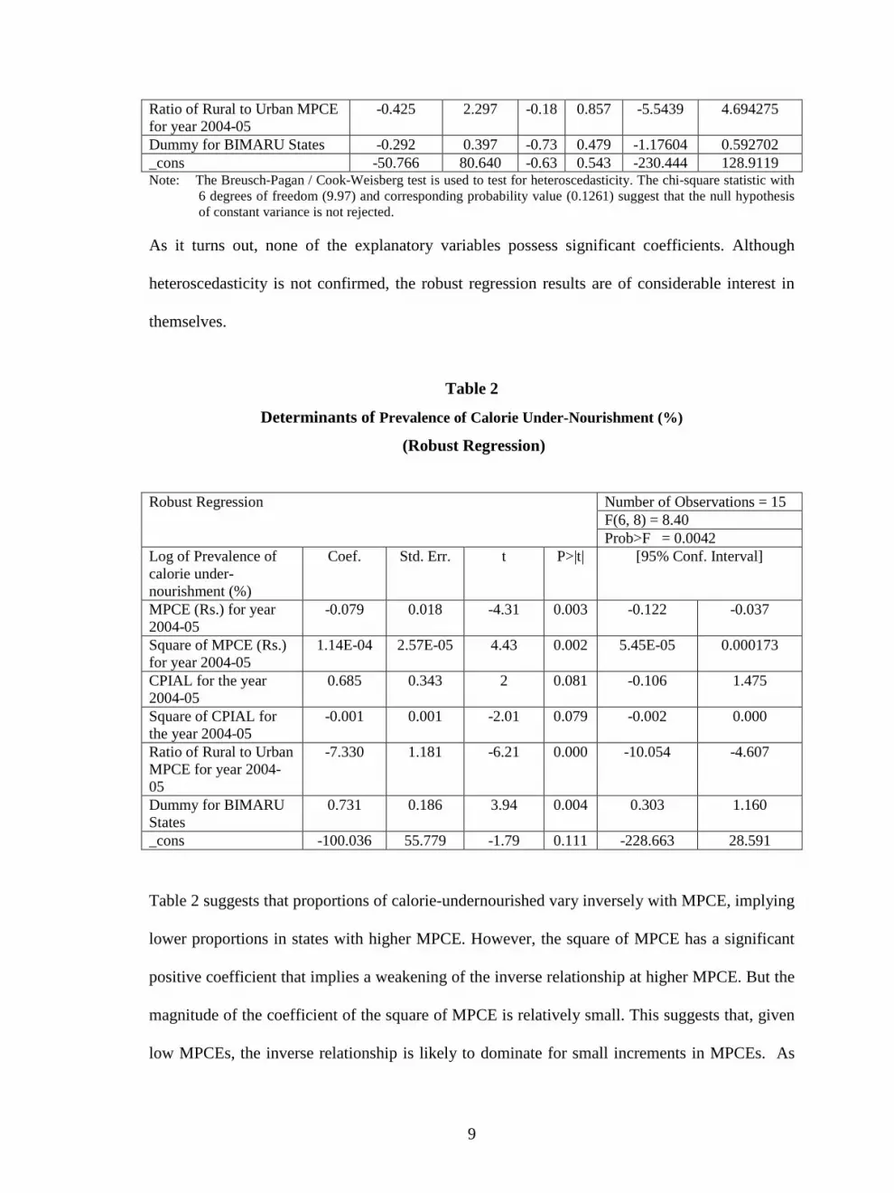
Table 2

Determinants of Prevalence of Calorie Under-Nourishment (%)

(Robust Regression)

Number of Observations = 15 F(6, 8) = 8.40

Robust Regression

Prob>F = 0.0042 Log of Prevalence of calorie under-nourishment (%)


MPCE (Rs.) for year 2004-05

-0.079 0.018 -4.31 0.003 -0.122 -0.037

Square of MPCE (Rs.) for year 2004-05

1.14E-04 2.57E-05 4.43 0.002 5.45E-05 0.000173

CPIAL for the year 2004-05

0.685 0.343 2 0.081 -0.106 1.475

Square of CPIAL for the year 2004-05

-0.001 0.001 -2.01 0.079 -0.002 0.000


-7.330 1.181 -6.21 0.000 -10.054 -4.607

Dummy for BIMARU States

0.731 0.186 3.94 0.004 0.303 1.160

_cons -100.036 55.779 -1.79 0.111 -228.663 28.591

Table 2 suggests that proportions of calorie-undernourished vary inversely with MPCE, implying

lower proportions in states with higher MPCE. However, the square of MPCE has a significant

positive coefficient that implies a weakening of the inverse relationship at higher MPCE. But the

magnitude of the coefficient of the square of MPCE is relatively small. This suggests that, given

low MPCEs, the inverse relationship is likely to dominate for small increments in MPCEs. As

10

expected, the higher the CPIAL, the greater is the prevalence of calorie-deficiency. However,

given the negative coefficient of (CPIAL)2, the positive effect of CPIAL diminishes at higher

values. This is presumably a result of substitution of cheaper sources of calorie19 . As

hypothesised, the lower the disparity between rural and urban MPCE, the lower is the proportion

of calorie-deficient population. This points to greater payoff to raising living standards in rural

areas, relatively to the urban. Somewhat surprisingly, in other specifications, offtake of PDS

does not have a significant negative effect20.

Controlling for all these effects, if a state belonged to the BIMARU group, the proportion of

undernourished would be higher. The overall specification is validated by the F-test.

The OLS and robust regression results on proportions of underweight children are given in

Tables 3 and 4, respectively. These are as hypothesised.

Table 3 Determinants of Proportion of Underweight among Children <5 years (%)

Number of Observations=17

Source SS df MS

F(2, 14) =14.97 Model 2.197 2 1.099 Prob>F = 0.0003

R-squared = 0.6814 Residual 1.027 14 0.073 Adj R-squared =0.6359

Total 3.224 16 0.202 Root MSE = .27087 Log of Proportion of Underweight among Children <5 years (%)


MPCE (Rs.) for the year 2004-05

-0.002 0.001 -2.13 0.051 -0.004 0.000

Female Literacy Rate -0.016 0.008 -2.04 0.061 -0.033 0.001 _cons 1.358 0.340 3.99 0.001 0.628 2.088

19 For a lucid and persuasive analysis, see Subramanian and Deaton, 1996. For an illustration of change of curvature in the Slutsky matrix, see Jha et al. 2009, following earlier contributions by Timmer, 1981, and Deolalikar and Behrman ,1987, 1988, 1989. 20 Details will be furnished on request.

11

Note: The Breusch-Pagan / Cook-Weisberg test is used to test for heteroscedasticity. The chi-square statistic with 2 degrees of freedom (0.90) and corresponding probability value (0.6378) suggest that the null hypothesis of constant variance is not rejected.

Table 4 Determinants of Proportion of Underweight among Children <5 years (%)

(Robust Regression)


Robust Regression

Prob>F = 0.0006 Log of Proportion of Underweight among Children <5 years (%)

Coef. Std. Err. T P>|t| [95% Conf. Interval]

MPCE (Rs.) for the year 2004-05

-0.002 0.001 -1.98 0.068 -0.004 0.000

Female Literacy Rate -0.016 0.008 -1.93 0.075 -0.034 0.002

_cons 1.338 0.360 3.71 0.002 0.565 2.110

The higher the MPCE, the lower was the prevalence of child undernutrition. Also, consistent

Table 5

Determinants of Under-five Mortality Rate (%)


Source SS df MS

F(5, 11) =21.83 Model 3.450 5 0.690 Prob>F = 0.0000

R-squared = 0.9085

Residual 0.348 11 0.032

Adj R-squared =0.8329

Total 3.798 16 0.237 Root MSE = 0.17777

Log of Under-five mortality rate (deaths per hundred)

Coef. Std. Err. T P>|t| [95% Conf. Interval]

CPIAL for the year 2003-04 0.002 0.005 0.40 0.698 -0.010 0.014 Delta of CPIAL for the year 2004-05 and 2003-04

0.011 0.005 2.45 0.032 0.001 0.021

Estimated Proportion of underweight among children <5 years without offtake (%)

0.019 0.012 1.57 0.144 -0.007 0.045

Lorenz Ratio in year 2004-05 0.313 0.115 2.72 0.020 0.059 0.566 Square of Lorenz Ratio in year 2004-05

-0.006 0.002 -3.09 0.010 -0.011 -0.002

_cons -7.853 2.291 -3.43 0.006 -12.895 -2.811 Note: The Breusch-Pagan / Cook-Weisberg test is used to test for heteroscedasticity. The chi-square statistic with


12

with earlier findings, female literacy significantly lowers undernutrition21. Both OLS and robust

regressions confirm these effects. The overall specification is validated by the F-test.

Let us now turn to the determinants of under-five mortality rates. As we prefer robust regression

results, we will confine our comments to Table 6. The higher the ∆ CPIAL (implying a reduction

in real MPCE), the higher is the under-five mortality rate. The higher the proportion of

underweight children, the higher is the mortality rate among under-five children. Recalling our

earlier remark about inequality/the Gini coefficient adding an important dimension to deprivation

(at the same level of MPCE), it is not surprising that there is a positive relationship between

under-five mortality and inequality. However, this relationship weakens because of the negative

Table 6

Determinants of Under-five Mortality Rate (%)

(Robust Regression)


Robust Regression

Prob>F = 0.0000 Log of Under-five mortality rate (deaths per hundred)


CPIAL for the year 2003-04 -0.003 0.005 -0.60 0.560 -0.015 0.009 Delta of CPIAL for the year 2004-05 and 2003-04

0.008 0.004 1.86 0.092 -0.002 0.017

Estimated Proportion of underweight among children <5 years without offtake (%)

0.029 0.011 2.61 0.026 0.004 0.053

Lorenz Ratio in year 2004-05

0.419 0.112 3.72 0.004 0.168 0.669

Square of Lorenz Ratio in year 2004-05

-0.007 0.002 -3.96 0.003 -0.012 -0.003

_cons -8.623 2.041 -4.22 0.002 -13.171 -4.074

coefficient of the square of the Gini.22 The overall specification is validated by the F-test.

21 Our experiments with CPIAL, and PDS offtake did not yield significant results. Details will be furnished on request.

13

(b) Undernutrition and Poverty

To further validate our econometric specifications and to link various indicators to poverty, some

graphs are given below.

Fig: 1Estimated and Actual Calorie Deficiency (%) by Headcount Ratio (%)

0

10

20

30

40

50

60

70

80

90

1008 14

15

15

18

20

21

23

24

25

31

33

37

39

42

42

46

Head Count Ratio (%)

Est

imat

ed a

nd A

ctua

l Cal

orie

Def

icie

ncy

(%)

Actual CalorieDeficiency (%)

Estimated CalorieDeficiency (%)

Except for two outliers in Fig: 1, generally the predicted values of prevalence of calorie

deficiency track closely the actual23. Another but somewhat surprising feature of this graph is

that there is no indication of a positive relationship between calorie deficiency and poverty.

22 Although somewhat outdated, Radhakrishna and Subbarao, 1997, estimated the cost (in rupees) per rupee of income transfer of five anti-poverty programmes to have been as follows during 1988–90: PDS, 5.37; rice subsidy scheme of the state of Andhra Pradesh, 6.35; a national employment programme for the poor, 4.34; the employment guarantee scheme of the state of Maharashtra 3.1; and Integrated Child Development Services, 1.8. On this, see also Srinivasan, 2000, and Gaiha and Kulkarni, 2006. 23 These are Kerala and Punjab. Both have low poverty rates but relatively high CPIAL.

14

0

10

20

30

40

50

60

70

8 15

18

21

24

31

37

42

46

Head Count Ratio (%)

Est

imat

ed a

nd A

ctua

l bel

ow F

ive

Chi

ld U

nder

wei

ght

(%)

Actual below FiveChild Underweight(%)

Estimated below FiveChild Underweight(%)

Fig: 2 Estimated and Actual below Five Child Underweight (%) vs Head Count Ratio (%)

By contrast, Fig: 2 not only portrays generally more accurate predictions but also a positive

relationship between the proportion of underweight children and poverty. In other words, the

more pervasive is poverty, the greater is the proportion of underweight children. Similarly in Fig:

3, the predicted mortality rates for under-five children follow closely the actual. Besides, there is

a positive relationship between mortality rate and poverty.

In sum, as discussed earlier, the determinants of different indicators of undernutrition vary. At

least two-proportion of underweight children and under-five mortality rate- rise with poverty.

(c) Analysis of Residuals

Following a standard practice, we investigate whether the residuals vary systematically with an

omitted variable. In various writings, Sen, 1997, and Dreze and Sen, 1989, have drawn attention

to the important role of the media in averting famines and mortality.

15

Fig: 3 Estimated and Actual Under Five Mortality (% ) by Headcount Ratio (% )

0

2

4

6

8

10

12

8

15

18

21

24

31

37

42

46

Head Count Ratio (% )

Est

imat

ed a

nd A

ctua

l Und

er F

ive

mor

tali

ty (%

)

Actual Under FiveMortality (%)

Estimated Under FiveMortality (%)

Accordingly, in Tables 7-12, we give the results of our analysis of the residuals of calorie

deficient population, underweight children under-five, and deaths of under-five children.

Table 7 Newspaper Circulation as a Determinant of Residuals of Prevalence of Calorie Under-

Nourishment (%)


Source SS df MS

F(2, 14) = 0.07 Model 103.21 2 51.60 Prob>F = 0.9315


Total 10239.28 16 639.96 Root MSE =26.907 Residuals of Prevalence of calorie under-nourishment (%)


Newspaper circulations (Lakh) 0.004 0.251 0.02 0.988 -0.534 0.542 Square of Newspaper circulations (Lakh)

0.000 0.001 0.11 0.914 -0.002 0.002

_cons -9.537 13.707 -0.70 0.498 -38.936 19.862 Note: The Breusch-Pagan / Cook-Weisberg test is used to test for heteroscedasticity. The chi-square statistic with


16

Table 8

Newspaper Circulation as a Determinant of Residuals of Prevalence of Calorie Under-

Nourishment (%) (Robust Regression)


Robust Regression

Prob>F = 0.8163 Residuals of Prevalence of calorie under-nourishment (%)


Newspaper circulations (Lakh)

0.010 0.019 0.55 0.591 -0.030 0.050

Square of Newspaper circulations (Lakh)

0.000 0.000 -0.63 0.540 0.000 0.000

_cons -0.321 1.015 -0.32 0.756 -2.498 1.856 Tables 7-8 confirm that there is no systematic relationship between prevalence of calorie

deficiency and newspaper circulation. This is perhaps not as surprising as hunger/undernutrition

in this form has no visible impact. Residuals of the other two indicators, however, display robust

relationships.

Table 9

Newspaper circulation as a Determinant of Residuals of Proportion of Underweight among Children <5 years (%)


Source SS df MS

F(2, 14) = 0.03 Model 2.48 2 1.24 Prob>F = 0.9707


Total 585.63 16 36.60 Root MSE =6.4539 Residuals of Proportion of Underweight among Children <5 years (%)


Newspaper circulations (Lakh) 0.014 0.060 0.24 0.813 -0.115 0.144 Square of Newspaper circulations (Lakh)

0.000 0.000 -0.21 0.833 0.000 0.000

_cons -0.512 3.288 -0.16 0.879 -7.563 6.540 Note: The Breusch-Pagan / Cook-Weisberg test is used to test for heteroscedasticity. The chi-square statistic with


17

Table 10, on the other hand, suggests that the residuals diminish with newspaper circulation but

at a slower rate. This implies that the greater the media exposure, the lower would be the gap

between the actual and predicted proportions of underweight children. In other words, the lower

would be the prospects of excess of actual proportion of underweight children. This evidence is

suggestive of the role of the media in averting child undernutrition-especially in its more visible

forms24.

Table 10

Newspaper Circulation as a Determinant of Residuals of Proportion of Underweight

among Children <5 years (%) (Robust Regression)


Robust Regression

Prob>F = 0.0501 Residuals of Proportion of Underweight among Children <5 years (%)



-0.152 0.078 -1.96 0.072 -0.320 0.016


0.001 0.000 2.53 0.025 0.000 0.002

_cons 3.582 3.203 1.12 0.284 -3.338 10.501

Table 11 Newspaper Circulation as a Determinant of Residuals of Under-five Mortality Rate (%)


Source SS Df MS

F(2, 14) = 3.80 Model 8.19 2 5.00 Prob>F = 0.0480


Total 23.28 16 1.45 Root MSE =1.038 Residuals of Under-five Mortality Rate (%)


Newspaper circulations (Lakh) -0.026 0.010 -2.64 0.019 -0.046 -0.005 Square of Newspaper circulations (Lakh)

0.000 0.000 2.76 0.015 0.000 0.000

_cons 1.397 0.529 2.64 0.019 0.263 2.531 Note: The Breusch-Pagan / Cook-Weisberg test is used to test for heteroscedasticity. The chi-square statistic with

2 degrees of freedom (11.82) and corresponding probability value (0.0027) suggest that the null hypothesis of constant variance is rejected at 1% level of significance.

24 For a recent comment, see Kapoor, 2009.

18

Both Tables 11-12 corroborate the important role of the media in averting the excess of child

mortality as well. More specifically, with higher newspaper circulation, the residuals decrease

but at a diminishing rate. Constrained by the data, we are unable to examine whether ‘local’

newspapers are more effective in performing this function than national newspapers.

Table 12

Newspaper Circulation as a Determinant of Residuals of Under-five Mortality Rate (%) (Robust Regression)


Robust Regression

Prob>F = 0.0201 Residuals of Under-five Mortality Rate (%)



-0.014 0.006 -2.41 0.030 -0.026 -0.002


0.000 0.000 2.99 0.010 0.000 0.000

_cons 0.559 0.313 1.78 0.096 -0.113 1.231

(e) Simulations

To illustrate policy priorities, counterfactual simulation results are summarised below.

• A 10 percent reduction in the (mean) CPIAL reduces prevalence of calorie deficiency

from 28.58 per cent to 17.31 per cent, a sharp reduction.

• If the (mean) MPCE rises by 10 per cent, the prevalence of calorie deficiency drops to

19.03 per cent.

• A reduction in rural –urban disparity-say, the ratio of rural MPCE to urban MPCE rises

by 10 per cent-reduces the prevalence to 20.34 per cent. An increase in the rural/urban

MPCE by 20 per cent reduces it to about 14 per cent.

19

• Turning to the proportion of underweight among under-five children, a 10 per cent higher

MPCE has a negligible effect – the (mean) proportion falls from 39.93 per cent to 38.05 per

cent.

• Somewhat surprisingly, the effect of higher female literacy is small too. A 10 per cent

higher female literacy reduces the proportion of underweight children to 37.66 per cent.

• If the increase in ∆ CPIAL is 10 per cent, the (mean) under-five mortality rate rises

slightly-from 6.88 per cent to 6.95 per cent. A 20 per cent higher value raises the mortality

rate to 7.02 per cent.

• If the proportion of underweight children falls by 10 per cent, the (mean) mortality rate

falls to 6.18 per cent; a 20 per cent reduction in the former reduces it to 5.55 per cent.

• Substantial reduction in income inequality, measured by the Gini coefficient, is

associated with sharp reduction in under-five mortality rate. If, for example, the Gini reduces

by 30 per cent-a substantial reduction that may not be feasible without a drastic reordering of

social and economic arrangements-the mortality rate drops to 5.15 per cent. If the Gini

reduces by 40 per cent, the mortality rate falls to 3.5 per cent.

In sum, MPCE alone is unlikely to reduce different forms of undernutrition. Reduction of

rural/urban disparity, consumer price stabilisation, and female literacy also play important

roles of varying degrees. Above all, conditional upon drastic social and economic

restructuring, substantial reduction in income inequality holds much potential for reducing

child mortality.

IV. Concluding Observations

Despite accelerated growth there is pervasive hunger, child undernutrition and mortality. In

fact, some of these indicators are the worst in the world. Our analysis focused on their

determinants.

20

If calorie deficiency is taken as a measure of hunger, its pervasiveness reflects low living

standards, high consumer prices, rural/urban disparity in living standards, and general

backwardness of a state (weak infrastructure, acute deprivation, and low literacy rates as in

BIMARU states).

Proportion of underweight five-year old children varies inversely with living standards, and

female literacy rate.

Under-five mortality rate varies inversely with increase in consumer prices, positively with

the proportion of underweight five-year old children, and non-linearly with the Gini of living

standards (i.e. positively with the Gini and negatively with the square of the Gini). But, in

general, except for calorie-deficiency prevalence, child undernutrition and mortality rise with

poverty. However, raising living standards alone will not reduce hunger and undernutrition.

Reduction of rural/urban disparities, consumer price stabilisation, mothers’ literacy have all

roles of varying importance in different nutrition indicators. Somewhat surprisingly, offtake

from the PDS does not have a significant effect on any of the three indicators considered

here.

Broadening the focus of the analysis, we examined the ‘excess’ of hunger and undernutrition

( i.e. the excess of actual over predicted values) as functions of media exposure (measured in

terms of newspaper circulation). Our analysis confirms that media exposure helps avert child

undernutrition and mortality. Indeed, the mass media have a key role in triggering public

action. The latter involves “not only food production and agricultural expansion, but also the

functioning of the entire economy, and even- more broadly –the operation of the political and

21

social arrangements that can, directly or indirectly, influence people’s ability to acquire food

and to achieve health and nourishment” (Sen, 1997, p. 23). If evidence is needed in support

of this view, it lies in a drastic reduction of economic inequality as a precondition for

reducing child mortality.

22

References

Behrman, J. and A. Deolalikar, 1987, “Will Developing Country Nutrition Improve with Income?

A Case Study for Rural South India”, Journal of Political Economy, vol. 95.

Behrman, J. and A. Deolalikar,1988 “Health and Nutrition”, in H. Chenery and T. N. Srinivasan

(eds.) Handbook of Development Economics, vol. 1, Amsterdam: Elsevier Science Publishers

B.V.

Behrman, J. and A. Deolalikar (1989) “Is Variety the Spice of Life? Implications for Calorie

Intake” Review of Economics and Statistics, vol. 71, no.4, pp. 666-672.

Bozzoli, C., A. Deaton, and C. Quintana-Domeque (2007) “ Child Mortality, Income and Adult

Height”, NJ: Princeton University, Research Programme in Development Studies, (mimeo).

Dasgupta, P. (1993). An Inquiry into Well-Being and Destitution. Oxford: Oxford

University Press.

Deaton, A. and J. Dreze (2002) “Poverty and Inequality in India: A Re-examination”, Economic

and Political Weekly, Vol 37, No 36, September 7.

Deaton, A. and J. Dreze (2008) “Nutrition in India: Facts and Interpretations”, (mimeo).

Dreze, J. and Amartya Sen (eds. 1990) The Political Economy of Hunger, vol. III, Oxford:

Clarendon Press.

Gaiha, R. (1999) “Food Prices and Income in India”, Canadian Journal of Development Studies,

vol. xx.

Gaiha, R. and Veena S. Kulkarni (2005) “Anthropometric Failure and Persistence of Poverty

in Rural India’, International Review of Applied Economics, Vol. 19, No. 2, 179–197.

Gaiha, R., G. Thapa, K. Imai and Vani S. Kulkarni “Has Anything Changed? Deprivation,

Disparity, and Discrimination in Rural India”, Brown Journal of World Affairs, vol. xiv, no.2.

Himanshu (2007) “Recent Trends in Poverty and Inequality: Some Preliminary Results”,

Economic and Political Weekly, 10 February.

23

Jha, R., R. Gaiha and A. Sharma (2009 a) “Mean Consumption, Poverty and Inequality in Rural

India in the Sixtieth Round of the National Sample Survey”, Journal of Asian and African

Studies, (forthcoming).

Jha, R., R. Gaiha and A. Sharma (2009 b) “Calorie and Micronutrient Deprivation and

Poverty- Nutrition Traps in Rural India”, World Development, May.

Jha, R., R. Gaiha and A. Sharma (2009 c) “On Modelling Variety in Consumption Expenditure

on Food”, International Review of Applied Economics, (forthcoming).

Jha, R., R. Gaiha and A. Sharma (2009 d) “Is There Curvature in the Slutsky Matrix-Analysis

with Indian Data”, draft.

Kapoor, C. (2009) “ Dealing with the Hidden Hunger of Our Children”, The Indian Express, 6

April.

Menon, P., A. Deolalikar and A. Bhaskar (2009) “India State Hunger Index: Comparisons of

Hunger Across States”, Washington DC: IFPRI.

Sen, Amartya (1997) “Hunger in the Contemporary World”, London: LSE-STICERD Research

Paper No. DEDPS 08.

Sridhar, D. (2008) The Battle against Hunger, New York: Oxford University Press.

Srinivasan, T. N. (1981) “Malnutrition: Some Measurement and Policy Issues”, Journal of

Development Economics, vol. 8.

Srinivasan, T. N. (1992) “Undernutrition: Concepts, Measurements and Policy Implications”, in

S. Osmani, (ed.) Nutrition and Poverty, Delhi: Oxford University Press.

Srinivasan, T. N. (1994) “Destitution: A Discourse”, Journal of Economic Literature, vol. 32.

Srinivasan, T. N. (2000) “Poverty and Undernutrition in South Asia”, Food Policy, vol. 25.

Strauss, J. and D. Thomas (1998) “Health, Nutrition, and Economic Development.”. Journal of

Economic Literature, Vol. 36, No. 2.

24

Subramaniam, S. and A. Deaton (1996) “The Demand for Food and Calories”, Journal of

Political Economy, vol. 1004, no.1.

Timmer, C. P. (1981)” Is There "Curvature" in the Slutsky Matrix?”, The Review of Economics

and Statistics, Vol. 63, No. 3 (Aug., 1981).

Annex

Table A.1. Definitions and Descriptive Statistics of Variables Used in the Analysis Variable Name Definitions N Mean SD Min Max

Dependent Variables Log of Prevalence of calorie under-nourishment (%)

Log of Prevalence of calorie under-nourishment (%) in 2005-06

17 -1.39 0.36 -2.08 -0.89

Log of Proportion of Underweight among Children <5 years (%)

Log of Proportion of Underweight among Children <5 years (%) in 2005-06

17 -0.40 0.45 -1.23 0.40

Log of Under-five mortality rate (deaths per hundred)

Log of Under-five mortality rate (deaths per hundred) in 2004-05

17 -2.70 0.49 -4.12 -2.24

Residuals of Prevalence of calorie under-nourishment (%)

Actual minus Estimated Prevalence of calorie under-nourishment (%)

17 -8.11 25.30 -83.03 10.28

Residuals of Proportion of Underweight among Children <5 years (%)

Actual minus Estimated Proportion of Underweight among Children <5 years (%)

17 0.19 6.05 -9.93 13.14

Residuals of Under-five Mortality Rate (%)

Actual minus Estimated Under-five Mortality Rate (%)

17 0.32 1.21 -0.75 4.15

Percentage off take in year 2003-04 Percentage off take in year 2003-04 17 53.71 22.82 9.02 86.63 Explanatory Variables

MPCE (Rs.) for year 2004-05 MPCE (Rs.) for year 2004-05 17 388.91 99.26 261.49 597.96 Square of MPCE (Rs.) for year 2004-05

Square of MPCE (Rs.) for year 2004-05

17 160522.5 85538.75 68376.97 357555.8



17 0.61 0.12 0.49 0.87

CPIAL for the year 2004-05 CPIAL for the year 2004-05 17 345.03 13.39 319.50 372.04 Square of CPIAL for the year 2004-05


17 119215.6 9180.74 102080.3 138415.0

CPIAL for the year 2003-04 CPIAL for the year 2003-04 17 330.93 13.54 311.00 348.75 Square of CPIAL for the year 2003-04


17 109690.3 8920.45 96721.00 121626.6

Delta of CPIAL for the year 2004-05 and 2003-04

CPIAL for the year 2004-05 minus CPIAL for the year 2003-04

17 14.10 11.86 -1.58 37.63

Dummy for BIMARU States 1 if States are Bihar, Madhya Pradesh, Rajasthan and Uttar Pradesh, 0 otherwise

17 0.24 0.44 0 1

Female Literacy Rate Female Literacy Rate of age 15-49 years in 2005-06

17 59.88 12.24 39.60 90.00

Lorenz Ratio in year 2004-05 Lorenz Ratio or Gini in year 2004-05 17 30.22 4.48 21.36 38.95 Square of Lorenz Ratio in year 2004-05

Square of Lorenz Ratio in year 2004-05

17 932.28 264.62 456.44 1517.33

Head Count Ratio (%) Head Count Ratio in year 2004-05 (%)

17 26.71 11.53 8.22 46.44

Square of Head Count Ratio (%) Square of Head Count Ratio in year 2004-05 (%)

17 838.68 653.47 67.57 2156.67

Estimated Proportion of underweight among children <5 years without offtake (%) (IV)

Estimated Proportion of underweight among children <5 years without offtake (%) (IV)

17 40.27 8.37 21.18 54.34

Newspaper circulations (Lakh) Newspaper circulations (Lakh) in 2005-06

17 83.81 81.27 9.04 332.92


Square of Newspaper circulations (Lakh) in 2005-06

17 13240.4 27015.27 81.67 110834.9

26

Endogeneity of Offtake of PDS

As food obtained from the PDS is likely to be greater when consumer prices are high, we

regress the former on CPIAl and (CPIAL)2. Both OLS and robust regression results point to a

non-linear relationship between offtake and CPIAL. At higher values of CPIAL, the negative

coefficient of CPIAL is more than offset by the positive coefficient of (CPIAL)2. Thus the

higher the CPIAL the greater is likely to be the offtake.

Table A.2

Determinants of Percentage Offtake of PDS in year 2003-04


Source SS df MS

F(2, 14) =1.61 Model 1556.868 2 778.434 Prob>F = 0.2349

R-squared = 0.1869 Residual 6772.619 14 483.759 Adj R-squared =0.0708

Total 8329.487 16 520.593 Root MSE = 21.995 Percentage off take in year 2003-04


CPIAL for the year 2003-04 -56.152 31.418 -1.79 0.096 -123.537 11.234 Square of CPIAL for the year 2003-04

0.085 0.048 1.79 0.095 -0.017 0.188

_cons 9275.832 5166.321 1.80 0.094 -1804.830 20356.490 Note: The Breusch-Pagan / Cook-Weisberg test is used to test for heteroscedasticity. The chi-square statistic with


Table A.2.1

Determinants of Percentage Offtake of PDS in year 2003-04 (Robust Regression)


Robust Regression

Prob>F = 0.0944 Percentage off take in year 2003-04


CPIAL for the year 2003-04

-75.995 32.078 -2.37 0.033 -144.796 -7.194


0.115 0.049 2.37 0.033 0.011 0.220

_cons 12557.480 5274.862 2.38 0.032 1244.030 23870.940

Documents

On Hunger and Child Mortality in India