Embed Size (px)
Citation preview
On numerical reconstructions of lithographic masks in DUVscatterometry
M.-A. Henn ∗a, R. Modela, M. Bara, M. Wurmb, B. Bodermannb, A. Rathsfeldc and H. Grossa
aPhysikalisch-Techn. Bundesanstalt, Abbestr. 2-12, D-10587 Berlin, Germany;bPhysikalisch-Techn. Bundesanstalt, Bundesallee 100, D-38116 Braunschweig, Germany;
cWeierstrass-Institute for Applied Analysis and Stochastics, Mohrenstr. 39, D-10117 Berlin,Germany
ABSTRACT
The solution of the inverse problem in scatterometry employing deep ultraviolet light (DUV) is discussed, i.e. weconsider the determination of periodic surface structures from light diffraction patterns. With decreasing dimen-sions of the structures on photo lithography masks and wafers, increasing demands on the required metrologytechniques arise. Scatterometry as a non-imaging indirect optical method is applied to periodic line structuresin order to determine the sidewall angles, heights, and critical dimensions (CD), i.e., the top and bottom widths.The latter quantities are typically in the range of tens of nanometers. All these angles, heights, and CDs are thefundamental figures in order to evaluate the quality of the manufacturing process. To measure those quantitiesa DUV scatterometer is used, which typically operates at a wavelength of 193 nm. The diffraction of light byperiodic 2D structures can be simulated using the finite element method for the Helmholtz equation. The corre-sponding inverse problem seeks to reconstruct the grating geometry from measured diffraction patterns. Fixingthe class of gratings and the set of measurements, this inverse problem reduces to a finite dimensional nonlinearoperator equation. Reformulating the problem as an optimization problem, a vast number of numerical schemescan be applied. Our tool is a sequential quadratic programing (SQP) variant of the Gauss-Newton iteration. Ina first step, in which we use a simulated data set, we investigate how accurate the geometrical parameters of anEUV mask can be reconstructed, using light in the DUV range. We then determine the expected uncertaintiesof geometric parameters by reconstructing from simulated input data perturbed by noise representing the esti-mated uncertainties of input data. In the last step, we use the measurement data obtained from the new DUVscatterometer at PTB to determine the geometrical parameters of a typical EUV mask with our reconstructionalgorithm. The results are compared to the outcome of investigations with two alternative methods namely EUVscatterometry and SEM measurements.
Keywords: DUV scatterometry, inverse problems, diffractive optics
1. INTRODUCTION
The structure geometries and dimensions of micro- or nano-structured surfaces can be investigated in a rapidand non-destructive way by the measurement and analysis of light diffraction due to the structured surfaces.In this context scatterometry plays an important role since it is not diffraction limited and can be used for theevaluation of structure dimensions on photo-masks and wafers in EUV lithography. While EUV scatterometry isthe only metrology that is capable to characterize the high reflecting MoSi-multilayer (MLS) of such a structure,DUV scatterometry can additionally be used for characterizations. Since it is nearly insensitive to modificationson the MLS it allows for an easy separation between absorber structure and multilayer features and a fastdetermination of profile properties such as the line to space ratio. At PTB a DUV hybrid scatterometer has beenrealized that operates at a wavelength of 193 nm. In order to deduce the grating topography from scatterometricmeasurements we need to solve the inverse grating diffraction problem. The software we use for this purposeis DIPOG,1 that has been developed by Weierstrass-Institute in Berlin. The paper is organized as follows: InSection 2 we shortly discuss the mathematical formulation of the scattering problem and the algorithms forsolving the inverse problem. Section 3 and 4 present an investigation that is based on a simulated data set
∗[email protected]; phone +49 30 3481 7784; www.ptb.de
Modeling Aspects in Optical Metrology II, edited by Harald Bosse, Bernd Bodermann, Richard M. Silver,Proc. of SPIE Vol. 7390, 73900Q · © 2009 SPIE · CCC code: 0277-786X/09/$18 · doi: 10.1117/12.827547
Proc. of SPIE Vol. 7390 73900Q-1
of how accurate the geometrical parameters of an EUV mask can be reconstructed, even for the case of noisymeasurement data. It is Section 5 where we apply our reconstruction algorithm to an actual set of measurementdata in order to determine the geometrical profile of an industrially manufactured EUV mask. Those results arefinally compared to earlier investigations for EUV and SEM measurements.
2. MATHEMATICAL FORMULATION OF THE SCATTERING PROBLEM
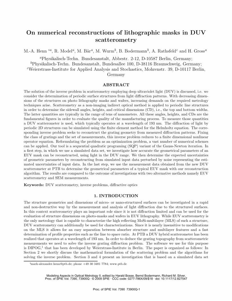
2.1 Scattering of EM Fields by a Periodic GratingScatterometry is the analysis of light diffracted by a periodic surface like the grating in Figure 1 below. Themathematical model for this phenomenon is based on Maxwell’s equations.2 Since geometry and material prop-erties are assumed to be invariant in one direction for such a grating, Maxwell’s equations in the time-harmoniccase reduce to the two-dimensional Helmholtz equation3
Δu(x, y) + k2u(x, y) = 0. (1)
Here u describes the transversal field component oscillating in the groove direction and k = k(x, y) = ω√
μ0ε(x, y)is the wave number, which is constant for the same material. In addition to the transmission conditions on theinterfaces between different domains and the quasi-periodic boundary conditions on the lateral boundaries theusual outgoing wave conditions are required in the infinite regions. The numerical solution is then found usingthe finite element method (FEM).4 DIPOG also contains a generalized FEM (GFEM) method for the case ofhighly oscillating fields.
Glass
MLS = 50 × [MoSi − Mo − MoSi − Mo]
SiSiO2
TaN
TaO(ARC)
p13 p12
p8 p7
p3 p2
p17 p16
top CD
bottom CD
period d
p11
p6
p1
x
y
z
Figure 1: Scheme of profile model of an EUV mask used in our studies.
2.2 Inverse Problem of scatterometryNow consider a given set of measured data, such as efficiencies or phase shift differences for different wavelengths,incident angles or polarization states, containing m elements denoted by {emeas
1 , . . . , emeasm }. Solving the inverse
problem means to determine an optical grating, whose diffraction patterns approximate the measurement datathe best, i.e. to find the optical and geometrical parameters {p1, . . . , pn} of the grating such that
‖E(p1, . . . , pn) − Emeas‖ = min. (2)
Proc. of SPIE Vol. 7390 73900Q-2
Here E is the nonlinear operator that maps the parameter vector (pi)i=1,...,n = p to the corresponding measure-ment data vector Emeas =
(emeas
j
)j=1,...,m
∈ Rm. The best approximation to (2) is found by minimizing the
weighted least-squares functional, known as the objective functional
Φ(p) := χ2(p) = ‖E(p) − Emeas‖2 =m∑
j=1
ωj
[ej(p) − emeas
j
]2. (3)
The ωj are weight factors, adjusted to the measurement uncertainties of the {emeasj }, see Section 4 below. All the
optimization algorithms implemented in DIPOG start with an initial value and operate iteratively. Beside fourgradient based local optimizers5, 6 there is also simulated annealing7 as a stochastic global optimizer. To avoidextremely time-consuming global optimization schemes to get the global minimum solution, a good starting guessis needed, or the numerical algorithm must be started from several initial solutions and the local solution withthe smallest functional value is declared the approximate global solution. There are however a lot of supportingtechniques that are helpful in finding the correct solution. Besides imposing feasible upper and lower bounds forthe reconstructed parameters, one can also choose proper weights within the objective functional or an optimalset of measurement data.8, 9 An algorithm to determine such a subset was also proposed in.9
3. RECONSTRUCTION WITH SIMULATED DATA
To get an impression of the accuracy of the reconstructed geometrical profile of an EUV mask , we use the datafrom simulated experiments as input for our optimization routine. Since the used EUV masks parameters areknown, we can compare the results of the reconstruction immediately to the ideal values. First results for theDUV reconstruction are given in.10
3.1 Design of EUV-mask and experimental setup
The set of data {emeas1 , . . . , emeas
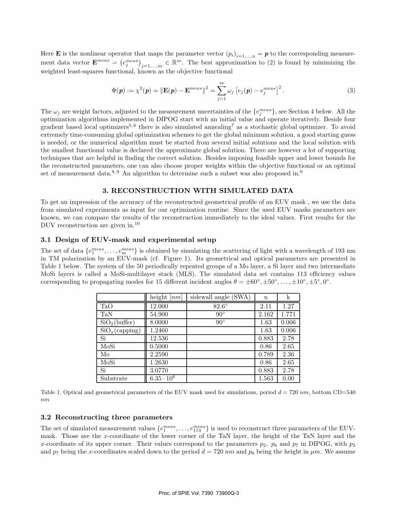
m } is obtained by simulating the scattering of light with a wavelength of 193 nmin TM polarization by an EUV-mask (cf. Figure 1). Its geometrical and optical parameters are presented inTable 1 below. The system of the 50 periodically repeated groups of a Mo layer, a Si layer and two intermediateMoSi layers is called a MoSi-multilayer stack (MLS). The simulated data set contains 113 efficiency valuescorresponding to propagating modes for 15 different incident angles θ = ±60◦,±50◦, . . . ,±10◦,±5◦, 0◦.
height [nm] sidewall angle (SWA) n kTaO 12.000 82.6◦ 2.11 1.27TaN 54.900 90◦ 2.162 1.771SiO2(buffer) 8.0000 90◦ 1.63 0.006SiOx(capping) 1.2460 1.63 0.006Si 12.536 0.883 2.78MoSi 0.5000 0.86 2.65Mo 2.2590 0.789 2.36MoSi 1.2630 0.86 2.65Si 3.0770 0.883 2.78Substrate 6.35 · 106 1.563 0.00
Table 1. Optical and geometrical parameters of the EUV mask used for simulations, period d = 720 nm, bottom CD=540nm
3.2 Reconstructing three parameters
The set of simulated measurement values {emeas1 , . . . , emeas
113 } is used to reconstruct three parameters of the EUV-mask. Those are the x-coordinate of the lower corner of the TaN layer, the height of the TaN layer and thex-coordinate of its upper corner. Their values correspond to the parameters p2, p6 and p7 in DIPOG, with p2
and p7 being the x-coordinates scaled down to the period d = 720 nm and p6 being the height in μm. We assume
Proc. of SPIE Vol. 7390 73900Q-3
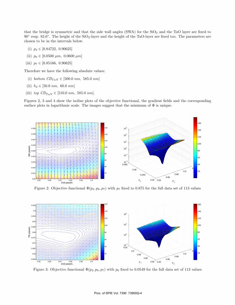
that the bridge is symmetric and that the side wall angles (SWA) for the SiO2 and the TaO layer are fixed to90◦ resp. 82.6◦. The height of the SiO2-layer and the height of the TaO-layer are fixed too. The parameters arechosen to be in the intervals below.
(i) p2 ∈ [0.84722, 0.90625]
(ii) p6 ∈ [0.0500 μm, 0.0600 μm]
(iii) p7 ∈ [0.85166, 0.90625]
Therefore we have the following absolute values:
(i) bottom CDTaN ∈ [500.0 nm, 585.0 nm]
(ii) h2 ∈ [50.0 nm, 60.0 nm]
(iii) top CDTaN ∈ [510.0 nm, 585.0 nm].
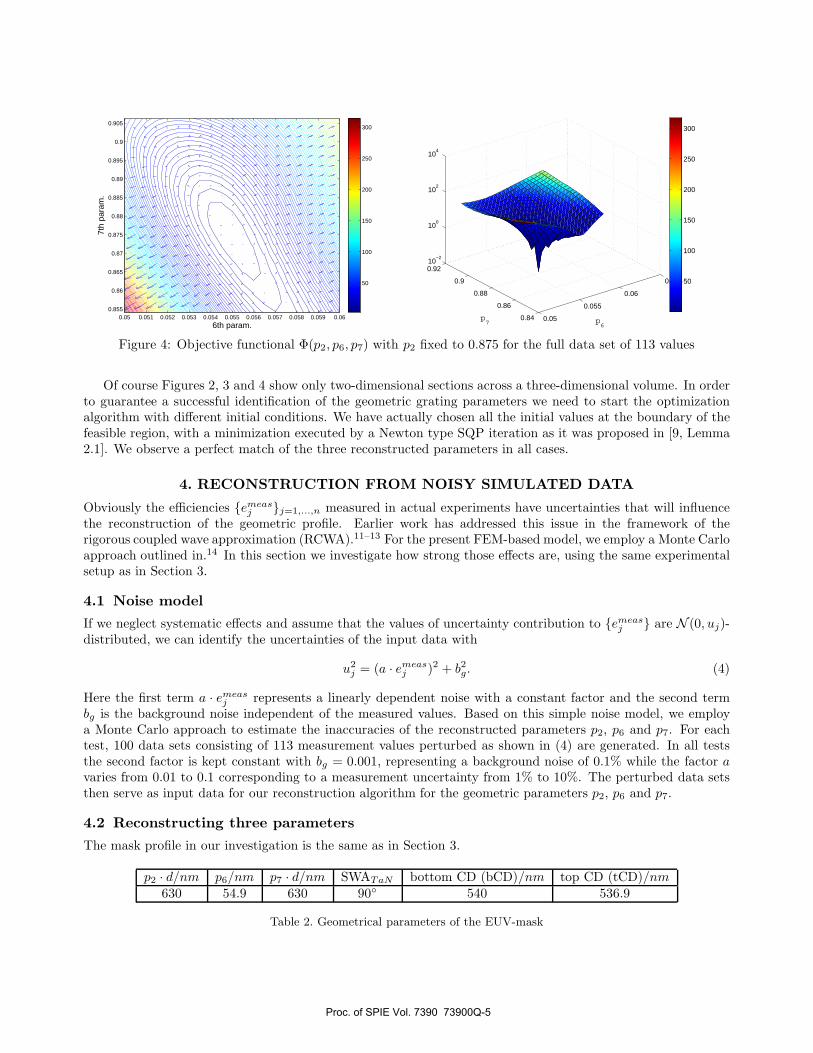
Figures 2, 3 and 4 show the isoline plots of the objective functional, the gradient fields and the correspondingsurface plots in logarithmic scale. The images suggest that the minimum of Φ is unique.
2nd param.
6th
para
m.
0.85 0.86 0.87 0.88 0.89 0.90.05
0.051
0.052
0.053
0.054
0.055
0.056
0.057
0.058
0.059
20
40
60
80
100
120
140
160
0.840.86
0.880.9
0.92
0.05
0.055
0.06
0.06510
−2
10−1
100
101
102
103
p2
p6
20
40
60
80
100
120
140
160
Figure 2: Objective functional Φ(p2, p6, p7) with p7 fixed to 0.875 for the full data set of 113 values
2nd param.
7th
para
m.
0.85 0.86 0.87 0.88 0.89 0.90.855
0.86
0.865
0.87
0.875
0.88
0.885
0.89
0.895
0.9
0.905
20
40
60
80
100
120
140
160
0.840.86
0.880.9
0.92
0.84
0.86
0.88
0.9
0.9210
−2
100
102
104
p2
p7
20
40
60
80
100
120
140
160
Figure 3: Objective functional Φ(p2, p6, p7) with p6 fixed to 0.0549 for the full data set of 113 values
Proc. of SPIE Vol. 7390 73900Q-4
6th param.
7th
para
m.
0.05 0.051 0.052 0.053 0.054 0.055 0.056 0.057 0.058 0.059 0.060.855
0.86
0.865
0.87
0.875
0.88
0.885
0.89
0.895
0.9
0.905
50
100
150
200
250
300
0.05
0.055
0.06
0.065
0.84
0.86
0.88
0.9
0.9210
−2
100
102
104
p6
p7
50
100
150
200
250
300
Figure 4: Objective functional Φ(p2, p6, p7) with p2 fixed to 0.875 for the full data set of 113 values
Of course Figures 2, 3 and 4 show only two-dimensional sections across a three-dimensional volume. In orderto guarantee a successful identification of the geometric grating parameters we need to start the optimizationalgorithm with different initial conditions. We have actually chosen all the initial values at the boundary of thefeasible region, with a minimization executed by a Newton type SQP iteration as it was proposed in [9, Lemma2.1]. We observe a perfect match of the three reconstructed parameters in all cases.
4. RECONSTRUCTION FROM NOISY SIMULATED DATA
Obviously the efficiencies {emeasj }j=1,...,n measured in actual experiments have uncertainties that will influence
the reconstruction of the geometric profile. Earlier work has addressed this issue in the framework of therigorous coupled wave approximation (RCWA).11–13 For the present FEM-based model, we employ a Monte Carloapproach outlined in.14 In this section we investigate how strong those effects are, using the same experimentalsetup as in Section 3.
4.1 Noise model
If we neglect systematic effects and assume that the values of uncertainty contribution to {emeasj } are N (0, uj)-
distributed, we can identify the uncertainties of the input data with
u2j = (a · emeas
j )2 + b2g. (4)
Here the first term a · emeasj represents a linearly dependent noise with a constant factor and the second term
bg is the background noise independent of the measured values. Based on this simple noise model, we employa Monte Carlo approach to estimate the inaccuracies of the reconstructed parameters p2, p6 and p7. For eachtest, 100 data sets consisting of 113 measurement values perturbed as shown in (4) are generated. In all teststhe second factor is kept constant with bg = 0.001, representing a background noise of 0.1% while the factor avaries from 0.01 to 0.1 corresponding to a measurement uncertainty from 1% to 10%. The perturbed data setsthen serve as input data for our reconstruction algorithm for the geometric parameters p2, p6 and p7.
4.2 Reconstructing three parameters
The mask profile in our investigation is the same as in Section 3.
p2 · d/nm p6/nm p7 · d/nm SWATaN bottom CD (bCD)/nm top CD (tCD)/nm630 54.9 630 90◦ 540 536.9
Table 2. Geometrical parameters of the EUV-mask
Proc. of SPIE Vol. 7390 73900Q-5
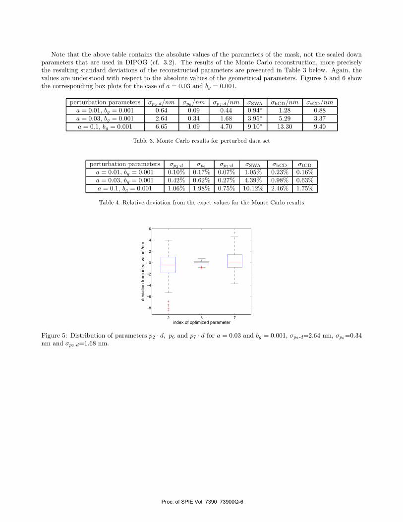
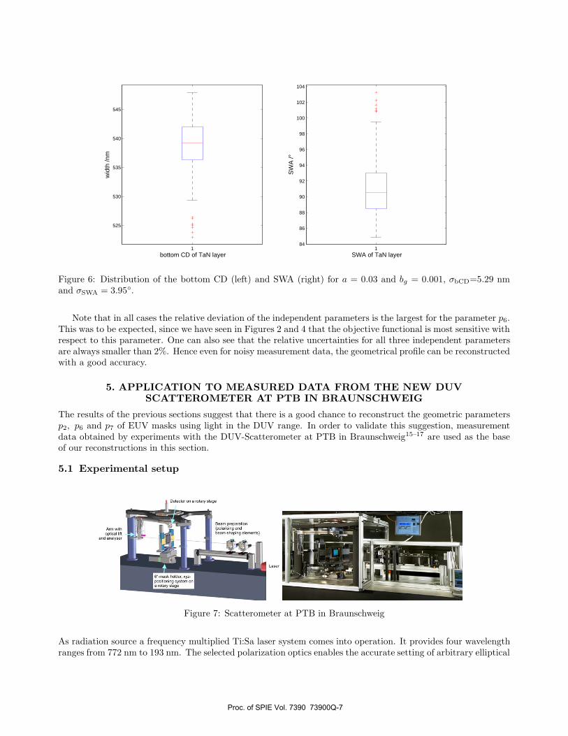
Note that the above table contains the absolute values of the parameters of the mask, not the scaled downparameters that are used in DIPOG (cf. 3.2). The results of the Monte Carlo reconstruction, more preciselythe resulting standard deviations of the reconstructed parameters are presented in Table 3 below. Again, thevalues are understood with respect to the absolute values of the geometrical parameters. Figures 5 and 6 showthe corresponding box plots for the case of a = 0.03 and bg = 0.001.
perturbation parameters σp2·d/nm σp6/nm σp7·d/nm σSWA σbCD/nm σtCD/nma = 0.01, bg = 0.001 0.64 0.09 0.44 0.94◦ 1.28 0.88a = 0.03, bg = 0.001 2.64 0.34 1.68 3.95◦ 5.29 3.37a = 0.1, bg = 0.001 6.65 1.09 4.70 9.10◦ 13.30 9.40
Table 3. Monte Carlo results for perturbed data set
perturbation parameters σp2·d σp6 σp7·d σSWA σbCD σtCD
a = 0.01, bg = 0.001 0.10% 0.17% 0.07% 1.05% 0.23% 0.16%a = 0.03, bg = 0.001 0.42% 0.62% 0.27% 4.39% 0.98% 0.63%a = 0.1, bg = 0.001 1.06% 1.98% 0.75% 10.12% 2.46% 1.75%
Table 4. Relative deviation from the exact values for the Monte Carlo results
2 6 7
−8
−6
−4
−2
0
2
4
6
devi
atio
n fr
om id
eal v
alue
/nm
index of optimized parameter
Figure 5: Distribution of parameters p2 · d, p6 and p7 · d for a = 0.03 and bg = 0.001, σp2·d=2.64 nm, σp6=0.34nm and σp7·d=1.68 nm.
Proc. of SPIE Vol. 7390 73900Q-6
Arm ssthoplical lift
and analyser
Dnteclor on a rotary stage
a-mask bolder, oyz-psaillaninasystern ora rotary stage
naarn preparation(potarining andbeam-shaping elements)
La
1
525
530
535
540
545w
idth
/nm
bottom CD of TaN layer1
84
86
88
90
92
94
96
98
100
102
104
SW
A /°
SWA of TaN layer
Figure 6: Distribution of the bottom CD (left) and SWA (right) for a = 0.03 and bg = 0.001, σbCD=5.29 nmand σSWA = 3.95◦.
Note that in all cases the relative deviation of the independent parameters is the largest for the parameter p6.This was to be expected, since we have seen in Figures 2 and 4 that the objective functional is most sensitive withrespect to this parameter. One can also see that the relative uncertainties for all three independent parametersare always smaller than 2%. Hence even for noisy measurement data, the geometrical profile can be reconstructedwith a good accuracy.
5. APPLICATION TO MEASURED DATA FROM THE NEW DUVSCATTEROMETER AT PTB IN BRAUNSCHWEIG
The results of the previous sections suggest that there is a good chance to reconstruct the geometric parametersp2, p6 and p7 of EUV masks using light in the DUV range. In order to validate this suggestion, measurementdata obtained by experiments with the DUV-Scatterometer at PTB in Braunschweig15–17 are used as the baseof our reconstructions in this section.
5.1 Experimental setup
Figure 7: Scatterometer at PTB in Braunschweig
As radiation source a frequency multiplied Ti:Sa laser system comes into operation. It provides four wavelengthranges from 772 nm to 193 nm. The selected polarization optics enables the accurate setting of arbitrary elliptical
Proc. of SPIE Vol. 7390 73900Q-7
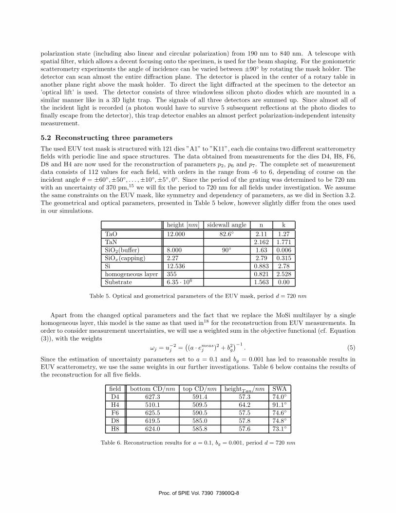
polarization state (including also linear and circular polarization) from 190 nm to 840 nm. A telescope withspatial filter, which allows a decent focusing onto the specimen, is used for the beam shaping. For the goniometricscatterometry experiments the angle of incidence can be varied between ±90◦ by rotating the mask holder. Thedetector can scan almost the entire diffraction plane. The detector is placed in the center of a rotary table inanother plane right above the mask holder. To direct the light diffracted at the specimen to the detector an’optical lift’ is used. The detector consists of three windowless silicon photo diodes which are mounted in asimilar manner like in a 3D light trap. The signals of all three detectors are summed up. Since almost all ofthe incident light is recorded (a photon would have to survive 5 subsequent reflections at the photo diodes tofinally escape from the detector), this trap detector enables an almost perfect polarization-independent intensitymeasurement.
5.2 Reconstructing three parameters
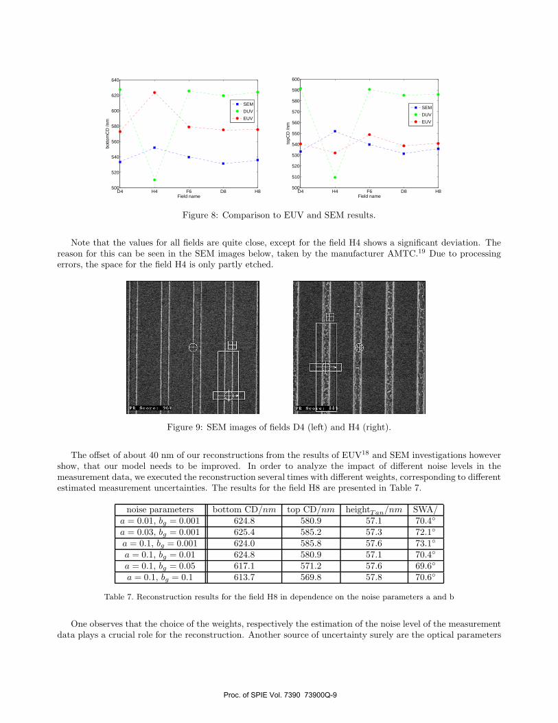
The used EUV test mask is structured with 121 dies ”A1” to ”K11”, each die contains two different scatterometryfields with periodic line and space structures. The data obtained from measurements for the dies D4, H8, F6,D8 and H4 are now used for the reconstruction of parameters p2, p6 and p7. The complete set of measurementdata consists of 112 values for each field, with orders in the range from -6 to 6, depending of course on theincident angle θ = ±60◦,±50◦, . . . ,±10◦,±5◦, 0◦. Since the period of the grating was determined to be 720 nmwith an uncertainty of 370 pm,15 we will fix the period to 720 nm for all fields under investigation. We assumethe same constraints on the EUV mask, like symmetry and dependency of parameters, as we did in Section 3.2.The geometrical and optical parameters, presented in Table 5 below, however slightly differ from the ones usedin our simulations.
height [nm] sidewall angle n kTaO 12.000 82.6◦ 2.11 1.27TaN 2.162 1.771SiO2(buffer) 8.000 90◦ 1.63 0.006SiOx(capping) 2.27 2.79 0.315Si 12.536 0.883 2.78homogeneous layer 355 0.821 2.528Substrate 6.35 · 106 1.563 0.00
Table 5. Optical and geometrical parameters of the EUV mask, period d = 720 nm
Apart from the changed optical parameters and the fact that we replace the MoSi multilayer by a singlehomogeneous layer, this model is the same as that used in18 for the reconstruction from EUV measurements. Inorder to consider measurement uncertainties, we will use a weighted sum in the objective functional (cf. Equation(3)), with the weights
ωj = u−2j =
((a · emeas
j )2 + b2g
)−1. (5)
Since the estimation of uncertainty parameters set to a = 0.1 and bg = 0.001 has led to reasonable results inEUV scatterometry, we use the same weights in our further investigations. Table 6 below contains the results ofthe reconstruction for all five fields.
field bottom CD/nm top CD/nm heightTan/nm SWAD4 627.3 591.4 57.3 74.0◦
H4 510.1 509.5 64.2 91.1◦
F6 625.5 590.5 57.5 74.6◦
D8 619.5 585.0 57.8 74.8◦
H8 624.0 585.8 57.6 73.1◦
Table 6. Reconstruction results for a = 0.1, bg = 0.001, period d = 720 nm
Proc. of SPIE Vol. 7390 73900Q-8
D4 H4 F6 D8 H8500
520
540
560
580
600
620
640
Field name
botto
mC
D /n
m
SEM
DUV
EUV
D4 H4 F6 D8 H8500
510
520
530
540
550
560
570
580
590
600
Field name
topC
D /n
m
SEM
DUV
EUV
Figure 8: Comparison to EUV and SEM results.
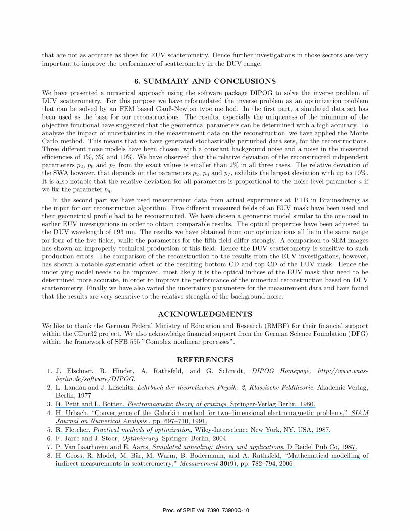
Note that the values for all fields are quite close, except for the field H4 shows a significant deviation. Thereason for this can be seen in the SEM images below, taken by the manufacturer AMTC.19 Due to processingerrors, the space for the field H4 is only partly etched.
Figure 9: SEM images of fields D4 (left) and H4 (right).
The offset of about 40 nm of our reconstructions from the results of EUV18 and SEM investigations howevershow, that our model needs to be improved. In order to analyze the impact of different noise levels in themeasurement data, we executed the reconstruction several times with different weights, corresponding to differentestimated measurement uncertainties. The results for the field H8 are presented in Table 7.
noise parameters bottom CD/nm top CD/nm heightTan/nm SWA/a = 0.01, bg = 0.001 624.8 580.9 57.1 70.4◦
a = 0.03, bg = 0.001 625.4 585.2 57.3 72.1◦
a = 0.1, bg = 0.001 624.0 585.8 57.6 73.1◦
a = 0.1, bg = 0.01 624.8 580.9 57.1 70.4◦
a = 0.1, bg = 0.05 617.1 571.2 57.6 69.6◦
a = 0.1, bg = 0.1 613.7 569.8 57.8 70.6◦
Table 7. Reconstruction results for the field H8 in dependence on the noise parameters a and b
One observes that the choice of the weights, respectively the estimation of the noise level of the measurementdata plays a crucial role for the reconstruction. Another source of uncertainty surely are the optical parameters
Proc. of SPIE Vol. 7390 73900Q-9
that are not as accurate as those for EUV scatterometry. Hence further investigations in those sectors are veryimportant to improve the performance of scatterometry in the DUV range.
6. SUMMARY AND CONCLUSIONS
We have presented a numerical approach using the software package DIPOG to solve the inverse problem ofDUV scatterometry. For this purpose we have reformulated the inverse problem as an optimization problemthat can be solved by an FEM based Gauß-Newton type method. In the first part, a simulated data set hasbeen used as the base for our reconstructions. The results, especially the uniqueness of the minimum of theobjective functional have suggested that the geometrical parameters can be determined with a high accuracy. Toanalyze the impact of uncertainties in the measurement data on the reconstruction, we have applied the MonteCarlo method. This means that we have generated stochastically perturbed data sets, for the reconstructions.Three different noise models have been chosen, with a constant background noise and a noise in the measuredefficiencies of 1%, 3% and 10%. We have observed that the relative deviation of the reconstructed independentparameters p2, p6 and p7 from the exact values is smaller than 2% in all three cases. The relative deviation ofthe SWA however, that depends on the parameters p2, p6 and p7, exhibits the largest deviation with up to 10%.It is also notable that the relative deviation for all parameters is proportional to the noise level parameter a ifwe fix the parameter bg.
In the second part we have used measurement data from actual experiments at PTB in Braunschweig asthe input for our reconstruction algorithm. Five different measured fields of an EUV mask have been used andtheir geometrical profile had to be reconstructed. We have chosen a geometric model similar to the one used inearlier EUV investigations in order to obtain comparable results. The optical properties have been adjusted tothe DUV wavelength of 193 nm. The results we have obtained from our optimizations all lie in the same rangefor four of the five fields, while the parameters for the fifth field differ strongly. A comparison to SEM imageshas shown an improperly technical production of this field. Hence the DUV scatterometry is sensitive to suchproduction errors. The comparison of the reconstruction to the results from the EUV investigations, however,has shown a notable systematic offset of the resulting bottom CD and top CD of the EUV mask. Hence theunderlying model needs to be improved, most likely it is the optical indices of the EUV mask that need to bedetermined more accurate, in order to improve the performance of the numerical reconstruction based on DUVscatterometry. Finally we have also varied the uncertainty parameters for the measurement data and have foundthat the results are very sensitive to the relative strength of the background noise.
ACKNOWLEDGMENTS
We like to thank the German Federal Ministry of Education and Research (BMBF) for their financial supportwithin the CDur32 project. We also acknowledge financial support from the German Science Foundation (DFG)within the framework of SFB 555 ”Complex nonlinear processes”.
REFERENCES1. J. Elschner, R. Hinder, A. Rathsfeld, and G. Schmidt, DIPOG Homepage, http://www.wias-
berlin.de/software/DIPOG.2. L. Landau and J. Lifschitz, Lehrbuch der theoretischen Physik: 2, Klassische Feldtheorie, Akademie Verlag,
Berlin, 1977.3. R. Petit and L. Botten, Electromagnetic theory of gratings, Springer-Verlag Berlin, 1980.4. H. Urbach, “Convergence of the Galerkin method for two-dimensional electromagnetic problems,” SIAM
Journal on Numerical Analysis , pp. 697–710, 1991.5. R. Fletcher, Practical methods of optimization, Wiley-Interscience New York, NY, USA, 1987.6. F. Jarre and J. Stoer, Optimierung, Springer, Berlin, 2004.7. P. Van Laarhoven and E. Aarts, Simulated annealing: theory and applications, D Reidel Pub Co, 1987.8. H. Gross, R. Model, M. Bar, M. Wurm, B. Bodermann, and A. Rathsfeld, “Mathematical modelling of
indirect measurements in scatterometry,” Measurement 39(9), pp. 782–794, 2006.
Proc. of SPIE Vol. 7390 73900Q-10

9. H. Gross and A. Rathsfeld, “Sensitivity analysis for indirect measurement in scatterometry and the re-construction of periodic grating structures,” Waves in Random and Complex Media 18(1), pp. 129–149,2008.
10. R. Model, A. Rathsfeld, H. Gross, M. Wurm, and B. Bodermann, “A scatterometry inverse problem inoptical mask metrology,” in J. Phys.: Conf. Ser., 135, 012071, Institute of Physics Publishing, 2008.
11. R. Al-Assaad and D. Byrne, “Error analysis in inverse scatterometry. I. Modeling,” Journal of the OpticalSociety of America A 24(2), pp. 326–338, 2007.
12. R. Silver, T. Germer, R. Attota, B. Barnes, B. Bunday, J. Allgair, E. Marx, and J. Jun, “Fundamental limitsof optical critical dimension metrology: A simulation study,” in Proceedings of SPIE, 6518, p. 65180U, 2007.
13. H. Patrick, T. Germer, R. Silver, and B. Bunday, “Developing an uncertainty analysis for optical scatterom-etry,” in Proceedings of SPIE, 7272, p. 72720T, 2009.
14. H. Gross, A. Rathsfeld, F. Scholze, R. Model, and M. Bar, “Computational methods estimating uncertaintiesfor profile reconstruction in scatterometry,” in Proceedings of SPIE, 6995, p. 69950T, 2008.
15. M.Wurm, Uber die dimensionelle Charakterisierung von Gitterstrukturen auf Fotomasken mit einem neuar-tigen DUV-Scatterometer. PhD thesis, Friedrich-Schiller-Universitat Jena, 2008.
16. M. Wurm, B. Bodermann, and F. Pilarski, “Metrology capabilities and performance of the new DUVscatterometer of the PTB,” in Proceedings of SPIE, 6533, p. 65330H, 2007.
17. M. Wurm, A. Diener, B. Bodermann, H. Gross, R. Model, and A. Rathsfeld, “Versatile DUV scatterometerof the PTB and FEM based analysis for mask metrology,” in Proceedings of SPIE, 6922, p. 692207, 2008.
18. H. Gross, A. Rathsfeld, F. Scholze, and M. Bar, “Profile reconstruction in EUV scatterometry: Modelingand uncertainty estimates,” WIAS Preprint (1411), 2009.
19. http://www.amtc-dresden.com.
Proc. of SPIE Vol. 7390 73900Q-11