s

c

-

f

s

l

t

s

-

.

On representing network heterogeneities in the incidencerate of simple epidemic models

Manojit Roy *, Mercedes Pascual

Department of Ecology and Evolutionary Biology, 830 North University Avenue, University of Michigan, Ann Arbor, MI 48109, United State

e c o l o g i c a l c om p l e x i t y 3 ( 2 0 0 6 ) 8 0 – 9 0

a r t i c l e i n f o

Article history:

Received 30 June 2005

Received in revised form

9 September 2005

Accepted 10 September 2005

Published on line 19 January 2006

Keywords:

Epidemics

SIRS

Network

Small-world

Fluctuations

Cycles

a b s t r a c t

Mean-field ecological models ignore space and other forms of contact structure. At the

opposite extreme, high-dimensional models that are both individual-based and stochasti

incorporate the distributed nature of ecological interactions. In between, moment approx

imations have been proposed that represent the effect of correlations on the dynamics o

mean quantities. As an alternative closer to the typical temporalmodels used in ecology, we

present here results on ‘‘modifiedmean-field equations’’ for infectious disease dynamics, in

which only mean quantities are followed and the effect of heterogeneous mixing i

incorporated implicitly. We specifically investigate the previously proposed empirica

parameterization of heterogeneousmixing inwhich the bilinear incidence rate SI is replaced

by a nonlinear term kSpIq, for the case of stochastic SIRS dynamics on different contac

networks, from a regular lattice to a random structure via small-world configurations. We

show that, for two distinct dynamical cases involving a stable equilibrium and a noisy

endemic steady state, the modifiedmean-field model approximates successfully the steady

state dynamics as well as the respective short and long transients of decaying cycles. Thi

result demonstrates that early on in the transients an approximate power-law relationship

is established between global (mean) quantities and the covariance structure in the net

work. The approach fails in the more complex case of persistent cycles observed within the

narrow range of small-world configurations.

# 2006 Elsevier B.V. All rights reserved

avai lable at www.sc iencedi rec t .com

journal homepage: ht tp : / /www.e lsev ier .com/ locate /ecocom

1. Introduction

Most population models of disease (Anderson and May, 1992)

assume complete homogeneous mixing, in which an indivi-

dual can interact with all others in the population. In these

well-mixed models, the disease incidence rate is typically

represented by the term bSI that is bilinear in S and I, the

number of susceptible and infective individuals (Bailey, 1975),

b being the transmission coefficient. With these models it has

been possible to establish many important epidemiological

results, including the existence of a population threshold for

the spread of disease and the vaccination levels required for

* Corresponding author. Present address: Department of Zoology, 22332611, United States. Tel.: +1 352 392 1040; fax: +1 352 392 3704.

E-mail addresses: roym@ufl.edu (M. Roy), pascual@umich.edu (M. P

1476-945X/$ – see front matter # 2006 Elsevier B.V. All rights reservedoi:10.1016/j.ecocom.2005.09.001

eradication (Kermack and McKendrick, 1927; Anderson and

May, 1992; Smith et al., 2005). However, individuals are

discrete and not well-mixed; they usually interact with only

a small subset of the population at any given time, thereby

imposing a distinctive contact structure that cannot be

represented inmean-fieldmodels. Explicit interactions within

discrete spatial and social neighborhoods have been incorpo-

rated into a variety of individual-based models on a spatial

grid and on networks (Bolker and Grenfell, 1995; Johansen,

1996; Rhodes and Anderson, 1996; Keeling, 1999; Pastor-

Satorras and Vespignani, 2001; Newman, 2002; Sander et al.,

2002; Van Baalen, 2002; Koopman, 2004; Shirley and Rushton,

Bartram Hall, PO Box 118525, University of Florida, Gainesville, FL

ascual).

d.

e c o l o g i c a l c om p l e x i t y 3 ( 2 0 0 6 ) 8 0 – 9 0 81

2005). Simplifications of these high-dimensional models

have been developed to better understand their dynamics,

make them more amenable to mathematical analysis and

reduce computational complexity (Keeling, 1999; Eames and

Keeling, 2002; Franc, 2004). These approximations are based

on moment closure methods and add corrections to the

mean-fieldmodel due to the influence of covariances, as well

as equations for the dynamics of these second order

moments (Pacala and Levin, 1997; Bolker, 1999; Brown and

Bolker, 2004).

We address here an alternative simplification approach

closer to the original mean-field formulation, which retains

the basic structure of the mean-field equations but incorpo-

rates the effects of heterogeneous mixing implicitly via

modified functional forms (McCallum et al., 2001). Specifically,

the bilinear transmission term (SI) in the well-mixed equa-

tions is replaced by a nonlinear term SpIq (Severo, 1969), where

the exponents p, q are known as ‘‘heterogeneity parameters’’.

This formulation allows an implicit representation of dis-

tributed interactions when the details of individual-level

processes are unavailable (as is often the case, see Gibson,

1997), and when field data are collected in the form of a time

series (e.g., Koelle and Pascual, 2004). We henceforth refer to

thesemodified equations as the heterogeneous mixing, or ‘‘HM’’,

model following Maule and Filipe (in preparation). The HM

model is known to exhibit important properties not observed

in standard mean-field models, such as the presence of

multiple equilibria and periodic solutions (Liu et al., 1986, 1987;

Hethcote and van den Driessche, 1991; Hochberg, 1991). This

model has also been successfully fitted to the experimental

time series data of lettuce fungal disease to explain its

persistence (Gubbins and Gilligan, 1997). However, it is not

well knownwhether thesemodifiedmean-field equations can

indeed approximate the population dynamics that emerge

from individual level interactions. Motivated by infectious

diseases of plants, Maule and Filipe (in preparation) have

recently compared the dynamics of the HM model to a

stochastic susceptible-infective (SI) model on a spatial lattice.

In this paper, we implement a stochastic version of the

susceptible-infective-recovered-susceptible (SIRS) dynamics,

to consider a broader range of dynamical behaviors including

endemic equilibria and cycles (Bailey, 1975; Murray, 1993;

Johansen, 1996). Recovery from disease leading to the

development of temporary immunity is also relevant to many

infectious diseases in humans, such as cholera (Koelle and

Pascual, 2004). For the contact structure of individuals in the

population we use a small-world algorithm, which is capable

of generating an array of configurations ranging from a regular

grid to a random network (Watts and Strogatz, 1998). Theory

on the structural properties of these networks is well

developed (Watts, 2003), and these properties are known to

exist in many real interaction networks (Dorogotsev and

Mendes, 2003). A small-world framework has also been used

recently to model epidemic transmission processes of severe

acute respiratory syndrome or SARS (Masuda et al., 2004;

Verdasca et al., 2005).

We demonstrate that the HM model can accurately

approximate the endemic steady states of the stochastic SIRS

system, including its short and long transients of damped

cycles under two different parameter regimes, for all config-

urations between the regular and random networks. We show

that this result implies the establishment early on in the

transients of a double power-law scaling relationship between

the covariance structure on the network and global (mean)

quantities at the population level (the total numbers of

susceptible and infective individuals). We also demonstrate

the existence of a complex dynamical behavior in the

stochastic system within the narrow small-world region,

consisting of persistent cycleswith enhanced amplitude and a

well-defined period that are not predicted by the equivalent

homogeneous mean-field model. In this case, the HM model

captures the mean infection level and the overall pattern of

the decaying transient cycles, but not their phases. Themodel

also fails to reproduce the persistence of the cycles. We

conclude by discussing the potential significance and limita-

tions of these observations.

2. The model

2.1. Stochastic formulation

2.1.1. The networkThe population structure, that is, the social contact pattern

among individuals in the population, is modeled using a

small-world framework as follows.We start with a spatial grid

with the interaction neighborhood restricted to eight neigh-

bors (Fig. 1A) and periodic boundary condition, and randomly

rewire a fraction f of the local connections (avoiding self and

multiple connections) such that the average number of

connections per individual is preserved at n0 (=8 in this case).

We call f the ‘‘short-cut’’ parameter of the network. This is a

two-dimensional extension of the algorithm described in

Watts and Strogatz (1998). As pointed out by Newman and

Watts (1999), a problemwith these algorithms is the small but

finite probability of the existence of isolated sub-networks.We

consider only those configurations that are completely

connected. For f = 0 we have a regular grid (Fig. 1A), whereas

f = 1 gives a random network (Fig. 1C). In between these

extremes, there is a range of f values near 0.01 within which

the network exhibits small-world properties (Fig. 1B). In this

region, most local connections remain intact making the

network highly ‘‘clustered’’ like the regular grid, with occa-

sional short-cuts that lower the average distance between

nodes drastically as in the random network. These properties

are illustratedwith two quantities, the ‘‘clustering coefficient’’

C and the ‘‘average path length’’ L (Watts, 2003). C denotes the

probability that two neighbors of a node are themselves

neighbor, and L denotes the average shortest distance

between two nodes in the network. The small-world network

exhibits the characteristic property of having a high value of C

and simultaneously a low value of L (Fig. 1D).

2.1.2. SIRS dynamicsOnce the network structure is generated using the algorithm

described above, the stochastic SIRS dynamics are imple-

mented with the following rules:

� A

susceptible individual gets infected at a rate nIb, where nIis the number of infective neighbors and b is the rate of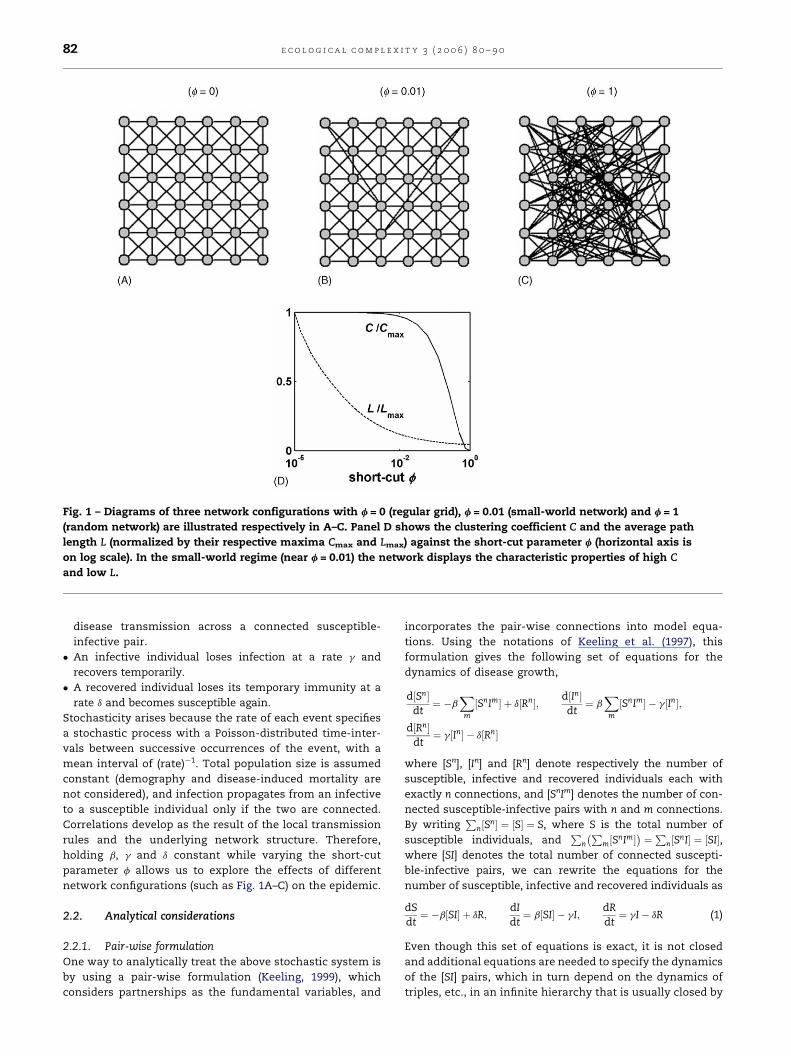

e c o l o g i c a l c om p l e x i t y 3 ( 2 0 0 6 ) 8 0 – 9 082

Fig. 1 – Diagrams of three network configurations with f = 0 (regular grid), f = 0.01 (small-world network) and f = 1

(random network) are illustrated respectively in A–C. Panel D shows the clustering coefficient C and the average path

length L (normalized by their respective maxima Cmax and Lmax) against the short-cut parameter f (horizontal axis is

on log scale). In the small-world regime (near f = 0.01) the network displays the characteristic properties of high C

and low L.

disease transmission across a connected susceptible-

infective pair.

� A

n infective individual loses infection at a rate g and

recovers temporarily.

� A

recovered individual loses its temporary immunity at a

rate d and becomes susceptible again.

Stochasticity arises because the rate of each event specifies

a stochastic process with a Poisson-distributed time-inter-

vals between successive occurrences of the event, with a

mean interval of (rate)�1. Total population size is assumed

constant (demography and disease-induced mortality are

not considered), and infection propagates from an infective

to a susceptible individual only if the two are connected.

Correlations develop as the result of the local transmission

rules and the underlying network structure. Therefore,

holding b, g and d constant while varying the short-cut

parameter f allows us to explore the effects of different

network configurations (such as Fig. 1A–C) on the epidemic.

2.2. Analytical considerations

2.2.1. Pair-wise formulationOne way to analytically treat the above stochastic system is

by using a pair-wise formulation (Keeling, 1999), which

considers partnerships as the fundamental variables, and

incorporates the pair-wise connections into model equa-

tions. Using the notations of Keeling et al. (1997), this

formulation gives the following set of equations for the

dynamics of disease growth,

d½Sn�dt

¼ �bXm

½SnIm� þ d½Rn�; d½In�dt

¼ bXm

½SnIm� � g½In�;

d½Rn�dt

¼ g½In� � d½Rn�

where [Sn], [In] and [Rn] denote respectively the number of

susceptible, infective and recovered individuals each with

exactly n connections, and [SnIm] denotes the number of con-

nected susceptible-infective pairs with n and m connections.

By writingP

n½Sn� ¼ ½S� ¼ S, where S is the total number of

susceptible individuals, andP

n

Pm½SnIm�

� �¼P

n½SnI� ¼ ½SI�,where [SI] denotes the total number of connected suscepti-

ble-infective pairs, we can rewrite the equations for the

number of susceptible, infective and recovered individuals as

dSdt

¼ �b½SI� þ dR;dIdt

¼ b½SI� � gI;dRdt

¼ gI� dR (1)

Even though this set of equations is exact, it is not closed

and additional equations are needed to specify the dynamics

of the [SI] pairs, which in turn depend on the dynamics of

triples, etc., in an infinite hierarchy that is usually closed by

e c o l o g i c a l c om p l e x i t y 3 ( 2 0 0 6 ) 8 0 – 9 0 83

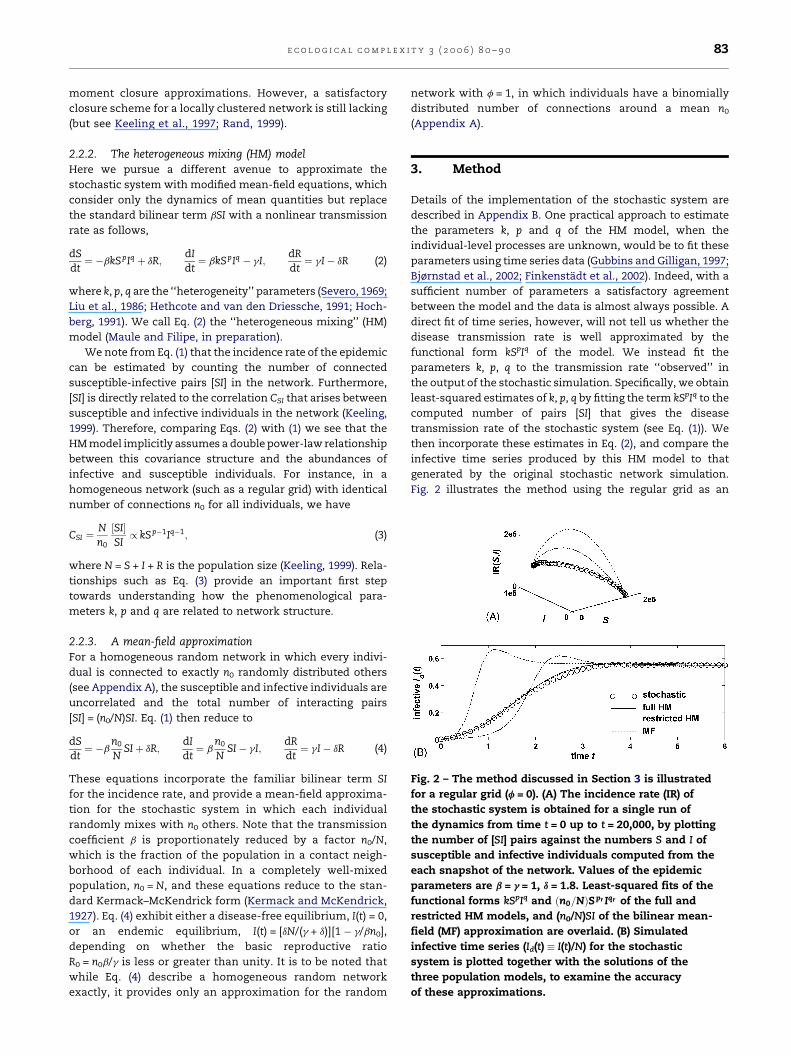
Fig. 2 – The method discussed in Section 3 is illustrated

for a regular grid (f = 0). (A) The incidence rate (IR) of

the stochastic system is obtained for a single run of

the dynamics from time t = 0 up to t = 20,000, by plotting

the number of [SI] pairs against the numbers S and I of

susceptible and infective individuals computed from the

each snapshot of the network. Values of the epidemic

parameters are b = g = 1, d = 1.8. Least-squared fits of the

functional forms kSpIq and ðn0=NÞSpr Iqr of the full and

restricted HM models, and (n0/N)SI of the bilinear mean-

field (MF) approximation are overlaid. (B) Simulated

infective time series (Id(t) � I(t)/N) for the stochastic

system is plotted together with the solutions of the

three population models, to examine the accuracy

of these approximations.

moment closure approximations. However, a satisfactory

closure scheme for a locally clustered network is still lacking

(but see Keeling et al., 1997; Rand, 1999).

2.2.2. The heterogeneous mixing (HM) modelHere we pursue a different avenue to approximate the

stochastic system with modified mean-field equations, which

consider only the dynamics of mean quantities but replace

the standard bilinear term bSI with a nonlinear transmission

rate as follows,

dSdt

¼ �bkSpIq þ dR;dIdt

¼ bkSpIq � gI;dRdt

¼ gI� dR (2)

where k, p, q are the ‘‘heterogeneity’’ parameters (Severo, 1969;

Liu et al., 1986; Hethcote and van den Driessche, 1991; Hoch-

berg, 1991). We call Eq. (2) the ‘‘heterogeneous mixing’’ (HM)

model (Maule and Filipe, in preparation).

We note from Eq. (1) that the incidence rate of the epidemic

can be estimated by counting the number of connected

susceptible-infective pairs [SI] in the network. Furthermore,

[SI] is directly related to the correlation CSI that arises between

susceptible and infective individuals in the network (Keeling,

1999). Therefore, comparing Eqs. (2) with (1) we see that the

HMmodel implicitly assumes a double power-law relationship

between this covariance structure and the abundances of

infective and susceptible individuals. For instance, in a

homogeneous network (such as a regular grid) with identical

number of connections n0 for all individuals, we have

CSI ¼N

n0

½SI�SI

/ kSp�1Iq�1; (3)

where N = S + I + R is the population size (Keeling, 1999). Rela-

tionships such as Eq. (3) provide an important first step

towards understanding how the phenomenological para-

meters k, p and q are related to network structure.

2.2.3. A mean-field approximationFor a homogeneous random network in which every indivi-

dual is connected to exactly n0 randomly distributed others

(see Appendix A), the susceptible and infective individuals are

uncorrelated and the total number of interacting pairs

[SI] = (n0/N)SI. Eq. (1) then reduce to

dSdt

¼ �bn0

NSIþ dR;

dIdt

¼ bn0

NSI� gI;

dRdt

¼ gI� dR (4)

These equations incorporate the familiar bilinear term SI

for the incidence rate, and provide a mean-field approxima-

tion for the stochastic system in which each individual

randomly mixes with n0 others. Note that the transmission

coefficient b is proportionately reduced by a factor n0/N,

which is the fraction of the population in a contact neigh-

borhood of each individual. In a completely well-mixed

population, n0 = N, and these equations reduce to the stan-

dard Kermack–McKendrick form (Kermack and McKendrick,

1927). Eq. (4) exhibit either a disease-free equilibrium, I(t) = 0,

or an endemic equilibrium, I(t) = [dN/(g + d)][1 � g/bn0],

depending on whether the basic reproductive ratio

R0 = n0b/g is less or greater than unity. It is to be noted that

while Eq. (4) describe a homogeneous random network

exactly, it provides only an approximation for the random

network with f = 1, in which individuals have a binomially

distributed number of connections around a mean n0(Appendix A).

3. Method

Details of the implementation of the stochastic system are

described in Appendix B. One practical approach to estimate

the parameters k, p and q of the HM model, when the

individual-level processes are unknown, would be to fit these

parameters using time series data (Gubbins and Gilligan, 1997;

Bjørnstad et al., 2002; Finkenstadt et al., 2002). Indeed, with a

sufficient number of parameters a satisfactory agreement

between the model and the data is almost always possible. A

direct fit of time series, however, will not tell us whether the

disease transmission rate is well approximated by the

functional form kSpIq of the model. We instead fit the

parameters k, p, q to the transmission rate ‘‘observed’’ in

the output of the stochastic simulation. Specifically, we obtain

least-squared estimates of k, p, q by fitting the term kSpIq to the

computed number of pairs [SI] that gives the disease

transmission rate of the stochastic system (see Eq. (1)). We

then incorporate these estimates in Eq. (2), and compare the

infective time series produced by this HM model to that

generated by the original stochastic network simulation.

Fig. 2 illustrates the method using the regular grid as an

e c o l o g i c a l c om p l e x i t y 3 ( 2 0 0 6 ) 8 0 – 9 084

example. In this way, we can address whether the transmis-

sion rate is well captured by themodified functional form, and

if that is the case, whether the HM model approximates

successfully the aggregated dynamics of the stochastic

system.

We compare the stochastic simulationwith the predictions

of three sets of model equations, representing different

degrees of approximation of the system. Besides the HM

model described above, we consider the bilinear mean-field

model given by Eq. (4), which assumes k = n0/N and p = q = 1.

This comparison demonstrates the inadequacy of the well-

mixed assumption built into the bilinear formulation. We also

discuss a restricted HM model with an incidence function of

the form ðn0=NÞSpr Iqr in Eq. (2), with only two heterogeneity

parameters pr and qr, as originally proposed by Severo (1969)

and studied by Liu et al. (1986), Hethcote and van den

Driessche (1991) and Hochberg (1991).

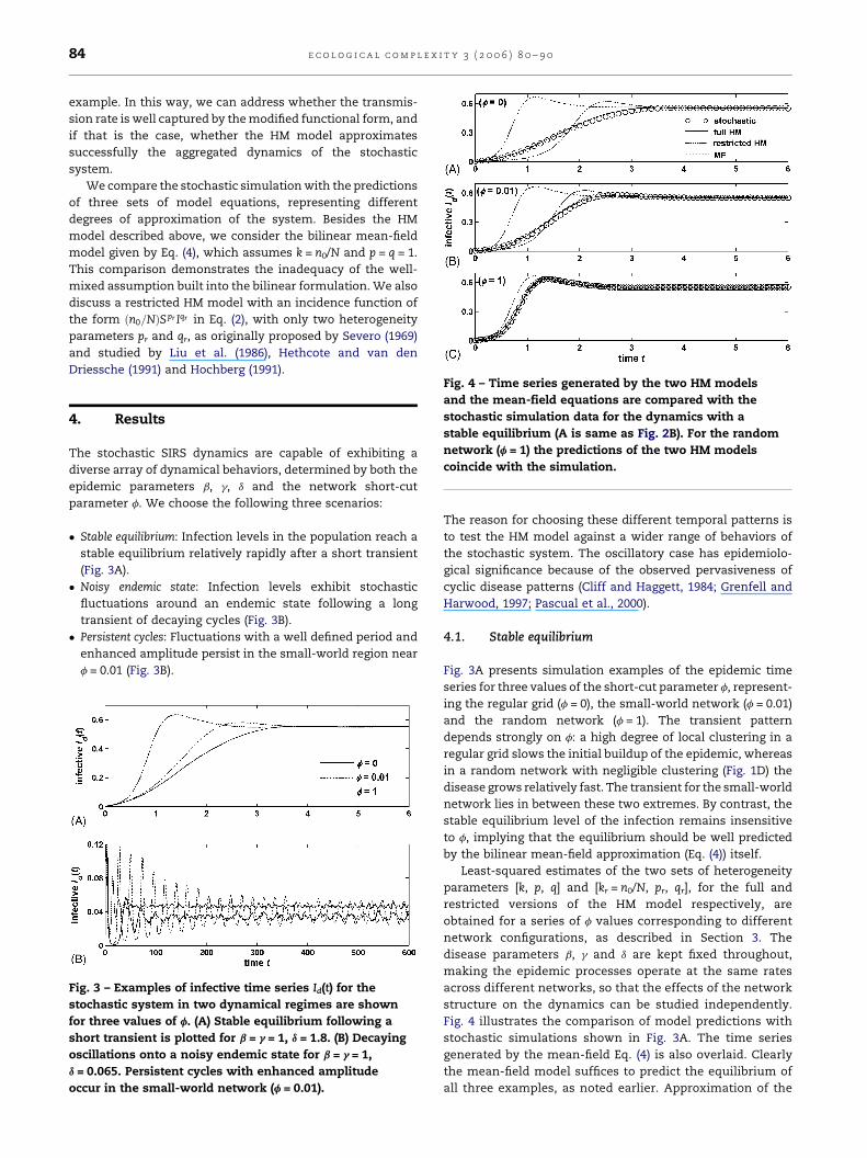
Fig. 4 – Time series generated by the two HM models

and the mean-field equations are compared with the

stochastic simulation data for the dynamics with a

stable equilibrium (A is same as Fig. 2B). For the random

network (f = 1) the predictions of the two HM models

coincide with the simulation.

4. Results

The stochastic SIRS dynamics are capable of exhibiting a

diverse array of dynamical behaviors, determined by both the

epidemic parameters b, g, d and the network short-cut

parameter f. We choose the following three scenarios:

� S

Fi

st

fo

sh

o

d

o

table equilibrium: Infection levels in the population reach a

stable equilibrium relatively rapidly after a short transient

(Fig. 3A).

� N

oisy endemic state: Infection levels exhibit stochastic

fluctuations around an endemic state following a long

transient of decaying cycles (Fig. 3B).

� P

ersistent cycles: Fluctuations with a well defined period and

enhanced amplitude persist in the small-world region near

f = 0.01 (Fig. 3B).

g. 3 – Examples of infective time series Id(t) for the

ochastic system in two dynamical regimes are shown

r three values of f. (A) Stable equilibrium following a

ort transient is plotted for b = g = 1, d = 1.8. (B) Decaying

scillations onto a noisy endemic state for b = g = 1,

= 0.065. Persistent cycles with enhanced amplitude

ccur in the small-world network (f = 0.01).

The reason for choosing these different temporal patterns is

to test the HM model against a wider range of behaviors of

the stochastic system. The oscillatory case has epidemiolo-

gical significance because of the observed pervasiveness of

cyclic disease patterns (Cliff and Haggett, 1984; Grenfell and

Harwood, 1997; Pascual et al., 2000).

4.1. Stable equilibrium

Fig. 3A presents simulation examples of the epidemic time

series for three values of the short-cut parameter f, represent-

ing the regular grid (f = 0), the small-world network (f = 0.01)

and the random network (f = 1). The transient pattern

depends strongly on f: a high degree of local clustering in a

regular grid slows the initial buildup of the epidemic, whereas

in a random network with negligible clustering (Fig. 1D) the

disease grows relatively fast. The transient for the small-world

network lies in between these two extremes. By contrast, the

stable equilibrium level of the infection remains insensitive

to f, implying that the equilibrium should be well predicted

by the bilinear mean-field approximation (Eq. (4)) itself.

Least-squared estimates of the two sets of heterogeneity

parameters [k, p, q] and [kr = n0/N, pr, qr], for the full and

restricted versions of the HM model respectively, are

obtained for a series of f values corresponding to different

network configurations, as described in Section 3. The

disease parameters b, g and d are kept fixed throughout,

making the epidemic processes operate at the same rates

across different networks, so that the effects of the network

structure on the dynamics can be studied independently.

Fig. 4 illustrates the comparison of model predictions with

stochastic simulations shown in Fig. 3A. The time series

generated by the mean-field Eq. (4) is also overlaid. Clearly

the mean-field model suffices to predict the equilibrium of

all three examples, as noted earlier. Approximation of the

e c o l o g i c a l c om p l e x i t y 3 ( 2 0 0 6 ) 8 0 – 9 0 85

Table 1 – Estimates of the parameters k, p and q for thefull HM model and different initial proportions ofinfective individuals in the population, for the case ofstochastic dynamics on a regular grid exhibiting stableequilibria (see text for details)

I0/N k p q

0.005 1.66 0.30 0.69

0.01 0.78 0.39 0.68

0.05 0.06 0.65 0.68

0.1 0.02 0.76 0.68

transient patterns, however, presents a different picture.

The mean-field trajectory deviates the most from the

stochastic simulation for the regular grid (f = 0), and the

least for the random network (f = 1). The full HM model with

its three parameters k, p and q, on the other hand,

demonstrates an excellent agreement with the stochastic

transients for all values of f. By comparison, the transient

patterns of the restricted HM model with only two fitting

parameters pr and qr differ significantly for low values of f

(Fig. 4A and B). The poor agreement of the restricted HM and

the mean-field transients with the stochastic data for a

clustered network (low f) is due to the failure of their

respective incidence functions to fit the transmission rate of

the stochastic system (Fig. 2A).

On the other hand, the random network has negligible

clustering, and the interaction between susceptible and

infective individuals is sufficiently well mixed for the

restricted HM model to provide as good an approximation

of the stochastic transient as the full HM model (Fig. 4C). The

estimates [k, p, q] = [0.0001, 0.94, 0.97] and [n0/N, pr,

qr] = [0.00005, 0.99, 1] for these two models are also quite

similar. The discrepancy for themean-field transients (Fig. 4C)

is due to the fact that the mean-field model gives only an

approximate description of the random network with f = 1 as

noted before. At the other extreme, for a regular grid the

estimates of the full and restricted HM models are [k, p,

q] = [1.66, 0.3, 0.69] and [n0/N, pr, qr] = [0.00005, 0.84, 1.13],which

differ considerably from each other.

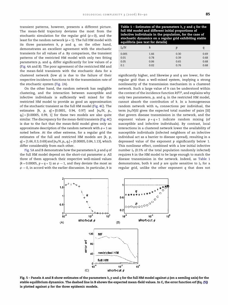
Fig. 5A and B demonstrate how the parameters k, p and q of

the full HM model depend on the short-cut parameter f. All

three of them approach their respective well-mixed values

(k = 0.00005, p = q = 1) as f ! 1, and they deviate the most as

f! 0, in accord with the earlier discussion. In particular, k is

Fig. 5 – Panels A and B show estimates of the parameters k, p and

stable equilibrium dynamics. The dashed line in B shows the exp

is plotted against f for the three epidemic models.

significantly higher, and likewise p and q are lower, for the

regular grid than a well-mixed system, implying a strong

nonlinearity of the transmission mechanism in a clustered

network. Such a large value of k can be understood within

the context of the incidence function kSpIq, and explains why

only two parameters, pr and qr in the restricted HM model,

cannot absorb the contribution of k. In a homogeneous

random network with n0 connections per individual, the

term (n0/N)SI gives the expected total number of pairs [SI]

that govern disease transmission in the network, and the

exponent values p = q = 1 indicate random mixing (of

susceptible and infective individuals). By contrast, local

interactions in a clustered network lower the availability of

susceptible individuals (infected neighbors of an infective

individual act as a barrier to disease spread), resulting in a

depressed value of the exponent p significantly below 1.

This nonlinear effect, combined with a low initial infective

number I0 (0.5% of the total population randomly infected)

requires k in the HM model to be large enough to match the

disease transmission in the network. Indeed, as Table 1

demonstrates, both k and p are quite sensitive to I0 for a

regular grid, unlike the other exponent q that does not

q for the full HMmodel against f (on a semilog axis) for the

ectedmean-field values. In C, the error function erf (Eq. (5))

e c o l o g i c a l c om p l e x i t y 3 ( 2 0 0 6 ) 8 0 – 9 086

depend on initial conditions. Increasing I0 facilitates disease

growth by distributing infective and susceptible individuals

more evenly, which causes an increase of the value of p and

a compensatory reduction of k.

An interesting pattern in Fig. 5A and B is that the values

of the heterogeneity parameters remain fairly constant

initially for low f, in particular within the interval

0 � f < 0.01 for the exponents p and q (the range is somewhat

shorter for k), and then start approaching respective mean-

field values as f increases to 1. This pattern of variation is

reminiscent of the plot for the clustering coefficient C shown

in Fig. 1D, and suggests that the clustering of the network,

rather than its average path length L, influences disease

transmission strongly.

A measure of the accuracy of the approximation can be

defined by an error function erf, computed as a mean of the

point-by-point deviation of the infective time series Im(t)

predicted from themodels, relative to the stochastic simulation

data Is(t), over the length T of the transient (the equilibrium

values of the models coincide with the simulation, see Fig. 4),

erf ¼ 1T

XTt¼1

jImðtÞ � IsðtÞjIsðtÞ

!� 100; (5)

(multiplication by 100 expresses erf as a percentage of the

simulation time series). Fig. 5C shows erf as a function of f for

the three models. The total failure of the mean-field approx-

imation to predict the stochastic transients is evident in the

large magnitudes of error (it is 25% even for the random

networks). By contrast, the excellent agreement of the full

HM model for all f results in a low error throughout. On the

other hand, the restricted version of the HM model gives over

30% error for low f whereas it is negligible for high f. Inter-

estingly, erf for the restrictedHMandmean-fieldmodels show

similar patterns of variation with f as in Fig. 5B, staying

relatively constant within 0 � f < 0.01 and then decreasing

relatively fast. Local clustering in a network with low f causes

disease transmission to deviate from a well-mixed approxi-

mation, and thus influences the pattern of erf for these sim-

pler models.

4.2. Stochastic fluctuations and persistent cycles

The second type of dynamical behavior of the stochastic

system exhibits a relatively long oscillatory transient that

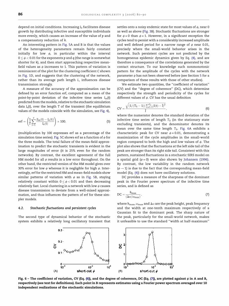
Fig. 6 – The coefficient of variation, CV (Eq. (6)), and the degree

respectively (see text for definitions). Each point in B represents e

independent realizations of the stochastic simulations.

settles onto a noisy endemic state for most values of f, near 0

as well as above (Fig. 3B). Stochastic fluctuations are stronger

for f = 0 than f = 1. However, in a significant exception the

cycles tend to persist with a considerably increased amplitude

and well defined period for a narrow range of f near 0.01,

precisely where the small-world behavior arises in the

network. Such persistent cycles are not predicted by the

homogeneous epidemic dynamics given by Eq. (4), and are

therefore a consequence of the correlations generated by the

contact structure. To our knowledge such nonmonotonic

pattern for the amplitude of the cycles with the network

parameter f has not been observed before (see Section 5 for a

comparison of these results with those of other studies).

We estimate two quantities, the ‘‘coefficient of variation’’

(CV) and the ‘‘degree of coherence’’ (DC), which determine

respectively the strength and periodicity of the cycles for

different values of f. CV has the usual definition

CV ¼

ffiffiffiffiffiffiffiffiffiffiffiffiffiffiffiffiffiffiffiffiffiffiffiffiffiffiffiffiffiffiffiffiffiffiffiffiffiffiffiffiffiffiffiffiffiffiffiffiffiffiffiffiffiffiffiffiffiffið1=ðTS � 1ÞÞ

PTSt¼1ðIðtÞ � IÞ2

qI

; (6)

where the numerator denotes the standard deviation of the

infective time series of length TS (in the stationary state

excluding transients), and the denominator denotes its

mean over the same time length TS. Fig. 6A exhibits a

characteristic peak for CV near f = 0.01, demonstrating a

maximization of the cycle amplitudes in the small-world

region compared to both the high and low values of f. The

plot also shows that the fluctuations at the left side tail of the

peak are stronger than its right side tail. Consistent with this

pattern, sustained fluctuations in a stochastic SIRS model on

a spatial grid (f = 0) were also shown by Johansen (1996).

By contrast, the low variability in the random network

(f ! 1) is due to the fact that the corresponding mean-field

model (Eq. (4)) does not have oscillatory solutions.

DC provides a measure of the sharpness of the dominant

peak in the Fourier power spectrum of the infective time

series, and is defined as

DC ¼ hmax

ðDv=vmaxÞ; (7)

where hmax, vmax and Dv are the peak height, peak frequency

and the width at one-tenth maximum respectively of a

Gaussian fit to the dominant peak. The sharp nature of

the peak, particularly for the small-world network, makes

it unfeasible to use the standard ‘‘width at half-maximum’’

of coherence, DC (Eq. (7)), are plotted against f in A and B,

stimates using a Fourier power spectrum averaged over 10

e c o l o g i c a l c om p l e x i t y 3 ( 2 0 0 6 ) 8 0 – 9 0 87

(Gang et al., 1993; Lago-Fernandez et al., 2000) which is often

zero here. The modified implementation in Eq. (7) therefore

considerably underestimates the sharpness of the dominant

peak. Even then, Fig. 6B depicts a fairly narrow maximum

for DC near f = 0.01, indicating that the cycles within the

small-world region have a well-defined period. The low

value of DC for f = 0 implies that the fluctuations in the

regular grid are stochastic in nature.

A likely scenario for the origin of these persistent cycles is

as follows. Stochastic fluctuations are locally maintained in

a regular grid by the propagating fronts of spatially

distributed infective individuals, but they are out of phase

across the network. The infective individuals are spatially

correlated over a length j / d�1 in the grid (Johansen, 1996),

which typically has a far shorter magnitude than the linear

extent of the grid used here (increasing d reduces the

correlation length j further, which weakens these fluctua-

tions and gives the stable endemic state observed for

instance in Fig. 3A). The addition of a small number of

short-cuts in a small-world network (Fig. 1B) couples

together a few of these local fronts, thereby effectively

increasing the correlation length to the order of the system

size and creating a globally coherent periodic response. As

more short-cuts are added, the network soon acquires a

sufficiently random configuration and the homogeneous

dynamics become dominant.

Another important point to note in Fig. 3B is that, in

contrast to Fig. 3A, the mean infection level I of the cycles is

not independent of f: I now increases slowly with f. An

immediate implication of this observation is that, unlike the

earlier case of a stable equilibrium, the bilinear mean-field

model of Eq. (4) will no longer be able to accurately predict

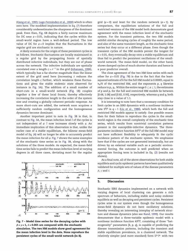
the mean infection for all f. Fig. 7 shows the same examples

of the stochastic time series as in Fig. 3B, along with the

solutions of the three models. As expected, the mean-field

time series fails to predict themean infection level at varying

degrees in all three cases, deviating most for the regular

Fig. 7 – Model time series for the decaying cycles with

b = g = 1, d = 0.065 are compared with the stochastic

simulation. The two HM models show good agreement for

the mean infection level in the data. None reproduce the

persistent cycles of the small-world network (in B).

grid (f = 0) and least for the random network (f = 1). By

comparison, the equilibrium solutions of the full and

restricted versions of the HM model both demonstrate good

agreement with the mean infection level of the stochastic

system. For the transient patterns, the two HM models

exhibit similar decaying cycles of roughly the same period,

and also of the same transient length, as the stochastic time

series but they occur at a different phase. Even though the

transient cycles of the HM models persist the longest for

f = 0.01, they eventually decay onto a stable equilibrium and

thus fail to predict the persistent oscillations of the small-

world network. The mean-field model, on the other hand,

shows damped cycles of much shorter duration and hence is

a poor predictor overall.

The close agreement of the two HM time series with each

other for f = 0.01 (Fig. 7B) is due to the fact that the least-

squared estimate of k for the full HMmodel is 0.00005, equal to

n0/N of the restricted HM, and the exponents p, q likewise

reduce to pr, qr.Within the entire range 0 � f � 1, the estimates

of p and pr for the full and restricted HM models lie between

[0.68, 1.08] and [0.82, 0.93], respectively, whereas q and qr both

stay close to a value of 1.1.

It is interesting to note here that a necessary condition for

limit cycles in an SIRS dynamics with a nonlinear incidence

rate SpIq is q > 1 (Liu et al., 1986), which both the full and

restricted HM models appear to satisfy. One possible reason

then for their failure to reproduce the cycles in the small-

world region is the overall complexity of the stochastic time

series, which results from nontrivial correlation patterns

present in the susceptible-infective dynamics. The three-

parameter incidence function kSpIq of the full HM model may

not have sufficient flexibility to adequately fit the cyclic

incidence pattern of the stochastic system. We emphasize

here that if the cycles are not generated intrinsically, but are

driven by an external variable such as a periodic environ-

mental forcing, the outcome is well predicted when an

appropriate forcing term is included in Eq. (2) (results not

shown).

As a final note, all of the above observations for both stable

equilibria and cyclic epidemic patterns have beenqualitatively

validated for multiple sets of values of the disease parameters

b, g and d.

5. Discussion

Stochastic SIRS dynamics implemented on a network with

varying degrees of local clustering can generate a rich

spectrum of behaviors, including stable and noisy endemic

equilibria as well as decaying and persistent cycles. Persistent

cycles arise in our system even though the homogeneous

mean-field dynamics do not have oscillatory solutions,

thereby revealing an interesting interplay of network struc-

ture and disease dynamics (also see Rand, 1999). Our results

demonstrate that a three-variable epidemic model with a

nonlinear incidence function kSpIq, consisting of three ‘‘het-

erogeneity’’ parameters [k, p, q], is capable of predicting the

disease transmission patterns, including the transient and

stable equilibrium prevalence, in a clustered network. The

relatively simpler (and more standard) form Spr Iqr with two

e c o l o g i c a l c om p l e x i t y 3 ( 2 0 0 6 ) 8 0 – 9 088

parameters [pr, qr] falls short in this regard. This restrictive

model, however, is an adequate predictor of the dynamics in a

random network, for which the bilinear mean-field approx-

imation cannot explain the transient pattern. Interestingly,

even the function kSpIq cannot capture the complex dynamics

of persistent cycles in a small-world network that has

simultaneously high local clustering and long-distance con-

nectivity. It is worth noting, however, that such persistent

cycles appear within a small region of the parameter space for

f, and therefore theHMmodel appears to provide a reasonable

approximation for most cases of clustered as well as

randomized networks.

An implication of these findings is that an approximate

relationship is established early on in the transients, lasting all

the way to equilibrium, between the covariance structure of

the [SI] pairs and the global (mean) quantities S and I. This

relationship is given by a double power law of the number of

susceptible and infective individuals. It allows the closure of

the equations for mean quantities, making it possible to

approximate the stochastic dynamics with a simple model

(HM) that mimics the basic formulation of the mean-field

equations but with modified functional forms. It reveals an

interesting scaling pattern from individual to population

dynamics, governed by the underlying contact structure of

the network. In lattice models for antagonistic interactions,

which bear a strong similarity to our stochastic disease

system, a number of power-law scalings have been described

for the geometry of the clusters (Pascual et al., 2002). It is an

open question whether the exponents for the dynamic scaling

(i.e., parameters p and q here) can be derived from such

geometrical properties. It also needs to be determined under

what conditions power-law relationships will hold between

local structure and global quantities.

The failure of the HM model to generate persistent cycles

may result from an inappropriate choice of the incidence

function kSpIq. It remains to be seen if there exists a different

functional form that better fits the incidence rate of the

stochastic system and is capable of predicting the variability

in the data. It is also not known whether a moment closure

method including the explicit dynamics of the covariance

terms themselves (Pacala and Levin, 1997; Keeling, 1999) can

provide a good approximation to the mean infection level in

a network with high degree of local clustering. Of course,

heterogeneities in space or in contact structure are not the

only factors contributing to the nonlinearity in the transmis-

sion function SpIq; a number of other biological mechanisms

of transmission can lead to such functional forms. By

rewriting bkSpIq as ½bkSp�1Iq�1�SI� bSI, where bðS; IÞ now

represents a density-dependent transmission efficiency in

the bilinear (homogeneous) incidence framework, one can

relate b to a variety of density-dependent processes such as

those involving vector-borne transmission, or threshold

virus loads etc (Liu et al., 1986). Interestingly, it has been

suggested that in such cases cyclic dynamics are likely to be

stabilized, rather than amplified, by nonlinear transmission

(Hochberg, 1991). It appears then that network structure can

contribute to the cyclic behavior of diseases with relatively

simple transmission dynamics.

It is interesting to consider the persistent cycles we have

discussed here in light of other studies on fluctuations in

networks. On one side, cycles have been described for random

networks with f = 1 because the corresponding well-mixed

dynamics also have oscillatory solutions (Lago-Fernandez

et al., 2000; Kuperman and Abramson, 2001). At the opposite

extreme, Johansen (1996) reported persistent fluctuations in a

stochastic SIRS model on a regular grid (f = 0), strictly

generated by the local clustering of the grid since the mean-

field equations do not permit cycles. Recent work by Verdasca

et al. (2005) extends Johansen’s observation by showing that

fluctuations do occur in clustered networks froma regular grid

to the small-world configuration. They describe a percolation

type transition across the small-world region, implying that

the fluctuations fall off sharply within this narro terval. This

observation is in significant contrast to our results, where the

amplitudes of the cycles are maximized by the small-world

configuration, and therefore require both local clustering and

some degree of randomization. One difference between the

two models is that Verdasca et al. (2005) use a discrete time

step for the recovery of infected individuals, while in our

event-drivenmodel, time is continuous and the recovery time

is exponentially distributed. A more systematic study of

parameter space for these models is warranted.

We should also mention that there are other ways to

generate a clustered network than a small-world algorithm.

For example, Keeling (2005) described a method that starts

with a number of randomly placed focal points in a two-

dimensional square, and draws a proportion of them towards

their nearest focal point to generate local clusters. Network

building can also be attempted from the available data on

selective social mixing (Morris, 1995). The advantage of our

small-world algorithm is that besides being simple to

implement, it is also one of the best studied networks (Watts,

2003). This algorithm generates a continuumof configurations

from a regular grid to a random network, and many real

systems have an underlying regular spatial structure, as in the

case of hantavirus of wild rats within the city blocks of

Baltimore (Childs et al., 1988). Moreover, emergent diseases

like the recent outbreak of severe acute respiratory syndrome

(SARS) have been studied by modeling human contact

patterns using small-world networks (Masuda et al., 2004;

Verdasca et al., 2005).

The network considered here remains static in time. While

this assumption is reasonable when disease spreads rapidly

relative to changes of the network itself, there are many

instances where the contact structure would vary over

comparable time scales. Examples include group dynamics

in wildlife resulting from schooling or spatial aggregation, as

well as territorial behavior. Dynamic network structure

involves processes such as migration among groups that

establishes new connections and destroys existing ones, but

also demographic processes such as birth and death as well as

disease induced mortality. Another topic of current interest is

the effect of predation on disease growth, which splices

together predator–prey andhost–pathogen dynamics inwhich

the prey is an epidemic carrier (Ostfeld and Holt, 2004). Simple

dynamics assuming the homogeneous mixing of prey and

predators makes interesting predictions about the harmful

effect of predator control in aggravating disease prevalence

with potential spill-over effects on humans (Packer et al., 2003;

Ostfeld and Holt, 2004). It remains to be seen if these

e c o l o g i c a l c om p l e x i t y 3 ( 2 0 0 6 ) 8 0 – 9 0 89

conclusions hold under an explicit modeling framework that

binds together the social dynamics of both prey and predator.

More generally, future work should address whether mod-

ified mean-field models provide accurate simplifications for

stochastic disease models on dynamic networks. So far the

work presented here for static networks provides support for

the empirical application of these simpler models to time

series data.

Acknowledgements

We thank Juan Aparicio for valuable comments about the

work, and Ben Bolker and an anonymous reviewer for useful

suggestions on the manuscript. This research was supported

by a Centennial Fellowship of the James S. McDonnell

Foundation to M.P.

Appendix A

A note on types of random networks

It is important to distinguish among the different types of

random networks that are used frequently in the literature.

One is the random network with f = 1 that is generated using

the small-world algorithm as described in Section 2 (Fig. 1C),

which has a total Nn0/2 distinct connections, where n0 is the

original neighborhood size (=8 here) in the regular grid andN is

the size of the network. Each individual in this random

network has a binomially distributed number of contacts

around a mean n0. There is also the homogeneous random

network discussed in relation to the mean-field Eq. (4), which

by definition has fixed n0 random contacts per individual

(Keeling, 1999). These two networks are, however, different

from the random network of Erdos and Renyi (Albert and

Barabasi, 2002), generated by randomly creating connections

with a probability p among all pairs of individuals in a

population. The expected number of distinct connections in

the population is then pN(N � 1)/2, and each individual has a

binomially distributed number of connections with mean

p(N � 1). For moderate values of p and large population sizes,

the Erdos–Renyi network is much more densely connected

than the first two types. All three of them, however, have

negligible clustering C and path length L, since the

individuals do not retain any local connections (all connec-

tions are short-cuts).

Appendix B

Details of model implementation

An appropriate network is constructed with a given f, and

the stochastic SIRS dynamics are implemented on this

network using the rules described in Section 2. For the initial

conditions, we start with a random distribution of a small

number of infective individuals, only 0.5% of the total

population (=0.005N) unless otherwise stated, in a pool of

susceptible individuals. All generated time series used for

least-squared fitting of the transmission rate have a length of

20,000 time units. The structure of the network remains fixed

during the entire stochastic run. Stochastic simulations were

carried outwith a series of network sizes ranging fromN = 104–

106. The results presented here are those for N = 160,000 and

are representative of other sizes. The values for the epidemic

rate parameters b, g and d are chosen so that the disease

successfully establishes in the population (a finite fraction of

the population remains infected at all times).

r e f e r e n c e s

Albert, R., Barabasi, A.L., 2002. Statistical mechanics of complexnetworks. Rev. Mod. Phys. 74, 47–97.

Anderson, R.M., May, R.M., 1992. Infectious Diseases of Humans:Dynamics and Control. Oxford University Press, Oxford.

Bailey, N.T., 1975. The Mathematical Theory of InfectiousDiseases. Griffin, London.

Bjørnstad, O.N., Finkenstadt, B.F., Grenfell, B.T., 2002. Dynamicsof measles epidemics: estimating scaling of transmissionrates using a time series SIR model. Ecol. Monogr. 72, 169–184.

Bolker, B.M., 1999. Analytic models for the patchy spread ofplant disease. Bull. Math. Biol. 61, 849–874.

Bolker, B.M., Grenfell, B., 1995. Space, persistence and dynamicsof measles epidemics. Philos. Trans. R. Soc. Lond. Ser. B 348,309–320.

Brown, D.H., Bolker, B., 2004. The effects of disease dispersaland host clustering on the epidemic threshold in plants.Bull. Math. Biol. 66, 341–371.

Childs, J.E., Glass, G.E., Korch, G.W., LeDuc, J.W., 1988. Theecology and epizootiology of hantaviral infections in smallmammal communities of Baltimore: a review andsynthesis. Bull. Soc. Vector Ecol. 13, 113–122.

Cliff, A.D., Haggett, P., 1984. Island epidemics. Sci. Am. 250, 138–147.

Dorogotsev, S.N., Mendes, J.F., 2003. Evolution of Networks.Oxford University Press, Oxford.

Eames, K.T.D., Keeling, M.J., 2002. Modelling dynamic andnetwork heterogeneities in the spread of sexuallytransmitted disease. PNAS 99, 13330–13335.

Finkenstadt, B.F., Bjørnstad, O.N., Grenfell, B.T., 2002. Astochastic model for extinction and recurrence ofepidemics: estimation and inference for measles outbreaks.Biostatistics 3, 493–510.

Franc, A., 2004. Metapopulation dynamics as a contact processon a graph. Ecol. Complex. 1, 49–63.

Gang, H., Ditzinger, T., Ning, C.Z., Haken, H., 1993. Stochasticresonance without external periodic force. Phys. Rev. Lett.71, 807–810.

Grenfell, B.T., Harwood, J., 1997. (Meta) population dynamics ofinfectious diseases. Trends Ecol. Evol. 12, 395–399.

Gubbins, S., Gilligan, C.A., 1997. A test of heterogeneous mixingas a mechanism for ecological persistence in a disturbedenvironment. Proc. R. Soc. Lond. B 264, 227–232.

Hethcote, H.W., van den Driessche, P., 1991. Someepidemiological models with nonlinear incidence. J. Math.Biol. 29, 271–287.

Hochberg, M.E., 1991. Non-linear transmission rates and thedynamics of infectious disease. J. Theor. Biol. 153, 301–321.

Johansen, A., 1996. A simple model of recurrent epidemics. J.Theor. Biol. 178, 45–51.

Keeling, M.J., Rand, D.A., Morris, A.J., 1997. Correlation modelsfor childhood epidemics. Proc. R. Soc. Lond. B 264, 1149–1156.

e c o l o g i c a l c om p l e x i t y 3 ( 2 0 0 6 ) 8 0 – 9 090

Keeling, M.J., 1999. The effects of local spatial structure onepidemiological invasions. Proc. R. Soc. Lond. B 266, 859–867.

Keeling, M.J., 2005. The implications of network structure forepidemic dynamics. Theor. Popul. Biol. 67, 1–8.

Kermack, W.O., McKendrick, A.G., 1927. A contribution to themathematical theory of epidemics. Proc. R. Soc. Lond. A 115,700–721.

Koelle, K., Pascual, M., 2004. Disentangling extrinsic fromintrinsic factors in disease dynamics: a nonlinear timeseries approach with an application to cholera. Am. Nat.163, 901–913.

Koopman, J., 2004. Modeling infection transmission. Ann. Rev.Pub. Health 25, 303–326.

Kuperman, M., Abramson, G., 2001. Small world effect in anepidemiological model. Phys. Rev. Lett. 86, 2909–2912.

Lago-Fernandez, L.F., Huerta, R., Corbacho, F., Siguenza, J.A.,2000. Fast response and temporal coherent oscillations insmall-world networks. Phys. Rev. Lett. 84, 2758–2761.

Liu, W., Levin, S.A., Iwasa, Y., 1986. Influence of nonlinearincidence rates upon the behavior of SIRS epidemiologicalmodels. J. Math. Biol. 23, 187–204.

Liu, W., Hethcote, H.W., Levin, S.A., 1987. Dynamical behavior ofepidemiological models with non-linear incidence rate. J.Math. Biol. 25, 359–380.

McCallum, H., Barlow, N., Hone, J., 2001. How should pathogentransmission be modelled? Trends Ecol. Evol. 16, 295–300.

Maule, M.M., Filipe, J.A.N., in preparation. Relatingheterogeneous mixing models to spatial processes indisease epidemics.

Masuda, N., Konno, N., Aihara, K., 2004. Transmission of severeacute respiratory syndrome in dynamical small-worldnetworks. Phys. Rev. E 69, 031917(1–6).

Morris, M., 1995. Data driven network models for the spread ofdisease. In: Mollison, D. (Ed.), Epidemic Models: TheirStructure and Relation to Data. Cambridge University Press,Cambridge, pp. 302–322.

Murray, J.D., 1993. Mathematical Biology. Springer-Verlag,Berlin.

Newman, M.E.J., 2002. The spread of epidemic disease onnetworks. Phys. Rev. E 66, 016128(1–11).

Newman, M.E.J., Watts, D.J., 1999. Scaling and percolation in thesmall-world network model. Phys. Rev. E 60, 7332–7342.

Ostfeld, R.S., Holt, R.D., 2004. Are predators good for yourhealth? Evaluating evidence for top-down regulation ofzoonotic disease reservoirs. Front. Ecol. Environ. 2, 13–20.

Pacala, S.W., Levin, S.A., 1997. Biologically generated spatialpattern and the coexistence of competing species. In:Tilman, D., Kareiva, P. (Eds.), Spatial Ecology. PincetonUniversity Press, Princeton, NJ, pp. 204–232.

Packer, C., Holt, R.D., Dobson, A., Hudson, P., 2003. Keepingthe herds healthy and alert: impacts of predation uponprey with specialist pathogens. Ecol. Lett. 6, 797–802.

Pascual, M., Rodo, X., Ellner, S.P., Colwell, R., Bouma, M.J., 2000.Cholera dynamics and EL Nino-Southern Oscillation.Science 289, 1766–1769.

Pascual, M., Roy, M., Franc, A., 2002. Simple temporal models forecological systems with complex spatial patterns. Ecol. Lett.5, 412–419.

Pastor-Satorras, R., Vespignani, A., 2001. Epidemic spreading inscale-free networks. Phys. Rev. Lett. 86, 3200–3203.

Rand, D.A., 1999. Correlation equations and pairapproximations for spatial ecologies. In: McGlade, J. (Ed.),Advanced Ecological Theory: Principles and Applications.Blackwell Sc., London, pp. 100–142.

Rhodes, C.J., Anderson, R.M., 1996. Persistence and dynamics inlattice models of epidemic spread. J. Theor. Biol. 180, 125–133.

Sander, L.M., Warren, C.P., Sokolov, I.M., Simon, C., Koopman, J.,2002. Percolation on heterogeneous networks as a model forepidemics. Math. Biosci. 180, 293–305.

Severo, N.C., 1969. Generalizations of some stochastic epidemicmodels. Math. Biosci. 4, 395–402.

Shirley, M.D.F., Rushton, S.P., 2005. The impacts of networktopology on disease spread. Ecol. Complex. 2, 287–299.

Smith, K.F., Dobson, A.P., McKenzie, F.E., Real, L.A., Smith, D.L.,Wilson, M.L., 2005. Ecological theory to enhance infectiousdisease control and public health policy. Front. Ecol.Environ. 3, 29–37.

Van Baalen, M., 2002. Contact networks and the evolution ofvirulence. In: Dieckmann, U., Metz, J.A.J., Sabelis, M.W.,Sigmund, K. (Eds.), Adaptive Dynamics of InfectiousDiseases. Cambridge University Press, Cambridge, pp.85–103.

Verdasca, J., Telo da Gama, M.M., Nunes, A., Bernardino, N.R.,Pacheco, J.M., Gomes, M.C., 2005. Recurrent epidemics insmall world networks. J. Theor. Biol. 233, 553–561.

Watts, D., 2003. Small Worlds. Princeton University Press,Princeton, NJ.

Watts, D.J., Strogatz, S., 1998. Collective dynamics of small-world networks. Nature 363, 202–204.