On representing signals using only timing informationRamdas Kumaresana) and Yadong WangDepartment of Electrical Engineering, Kelley Hall, 4 East Alumni Avenue, University of Rhode Island,Kingston, Rhode Island 02881

~Received 7 December 1999; revised 20 July 2001; accepted 1 August 2001!

It is well known that only a special class of bandpass signals, called real-zero~RZ! signals can beuniquely represented~up to a scale factor! by their zero crossings, i.e., the time instants at which thesignals change their sign. However, it is possible to invertibly map arbitrary bandpass signals intoRZ signals, thereby, implicitly represent the bandpass signal using the mapped RZ signal’s zerocrossings. This mapping is known as real-zero conversion~RZC!. In this paper a class of novelsignal-adaptive RZC algorithms is proposed. Specifically, algorithms that are analogs of well-knownadaptive filtering methods to convert an arbitrary bandpass signal into other signals, whose zerocrossings contain sufficient information to represent the bandpass signal’s phase and envelope arepresented. Since the proposed zero crossings arenot those of the original signal, but only indirectlyrelated to it, they are called hidden or covert zero crossings~CoZeCs!. The CoZeCs-basedrepresentations are developed first for analytic signals, and then extended to real-valued signals.Finally, the proposed algorithms are used to represent synthetic signals and speech signals processedthrough an analysis filter bank, and it is shown that they can be reconstructed given the CoZeCs.This signal representation has potential in many speech applications. ©2001 Acoustical Society ofAmerica. @DOI: 10.1121/1.1405523#

PACS numbers: 43.60.Lq, 43.72.Ar, 43.64.Bt@JCB#

f aigh

o

ro

erarrev

m

a

nge,nch

coot

thengof

efs.als-n-eno-delWerateowin-

he

l are

u--

--

der

d

nd-

I. INTRODUCTION

A key issue in sampling theory is the construction osequence of samples that unambiguously represent a ss(t). There are two major approaches to constructing sucsequence of samples.1

~1! The first is the familiar ‘‘Shannon sampling,’’2 i.e.,define samples$sn% as the values taken bys(t) on a given setof sampling points,$tn%, i.e., sn5s(tn).

~2! The second approach is the less familiar notionrepresenting signals by certain time instants...,t21 ,t0 ,t1 ,t2 ,... . Specifically, for example, in certain cases the zecrossings or level-crossing locations ofs(t) can be used torepresents(t) to within a scale factor.

Reconstruction is the process of the pointwise recovof s(t) given the sampling sequence. In this paper weprimarily concerned with the second approach, i.e., repsenting bandpass signals by certain time instants. Howein the proposed signal representation schemes, these tiinstants are not the zero-crossing locations ofs(t) them-selves~as in, for example, Refs. 3, 4!, but the zero-crossinglocations of certain functions that are related to the phaseenvelope of the signals(t).

A motivation for signal representation based on timiinstants comes from our desire to understand certain aspof biological signal processing. The cochlea, or inner earknown to decompose an acoustic stimulus into frequecomponents along the length of the basilar membrane. Tphenomenon is called atonotopicdecomposition.5 Further, itis also known that the nerve fibers emanating from thechlea convey information to the brain in the form of trainsalmost identically shaped nerve impulses or spikes. Since

a!Electronic mail: kumar@ele.uri.edu

J. Acoust. Soc. Am. 110 (5), Pt. 1, Nov. 2001 0001-4966/2001/110(5)/2

nala

f

-

ye-

er,ing

nd

ctsisyis

-fhe

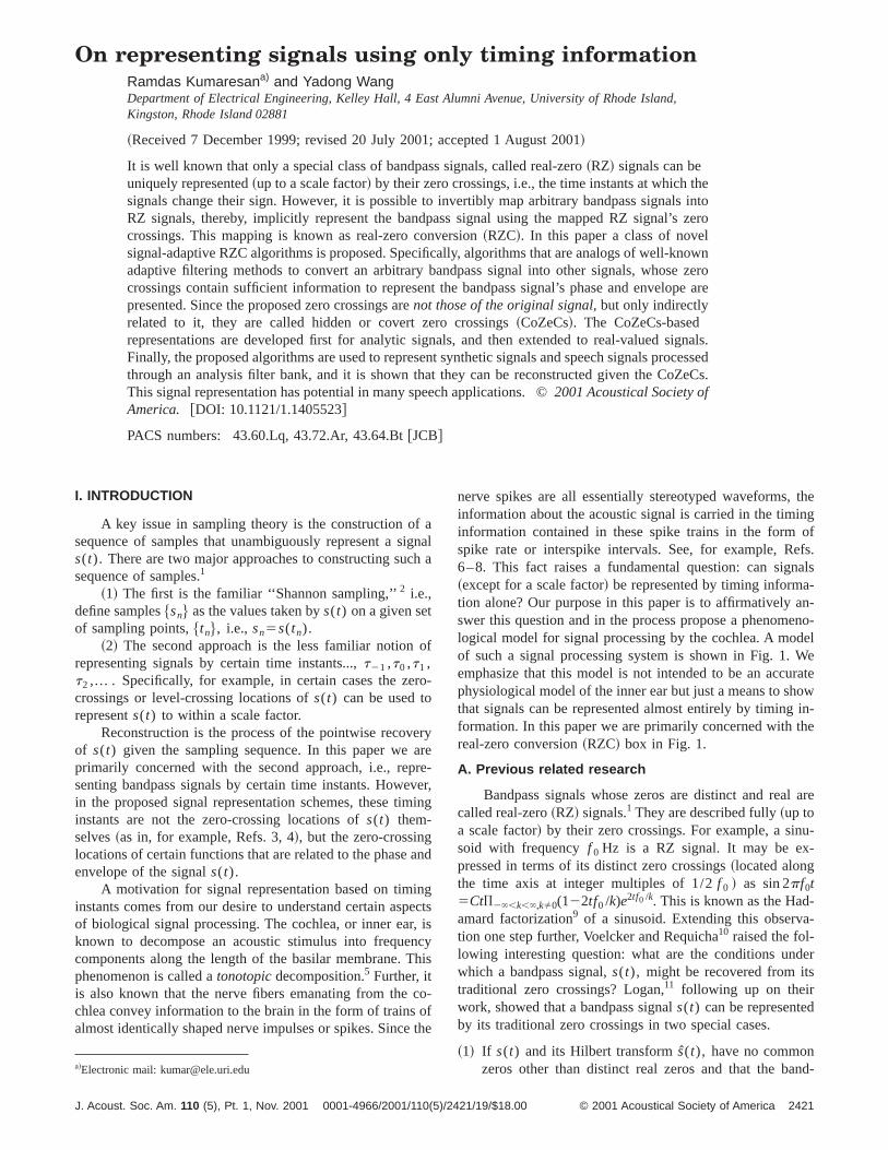
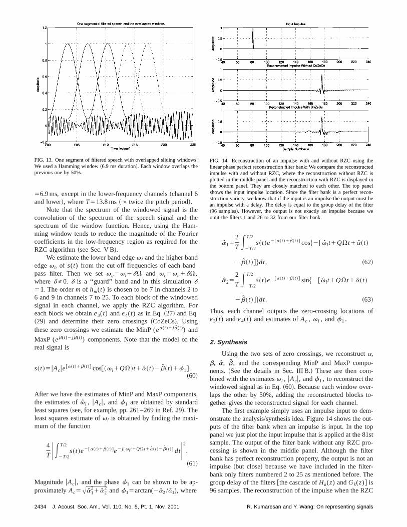
nerve spikes are all essentially stereotyped waveforms,information about the acoustic signal is carried in the timiinformation contained in these spike trains in the formspike rate or interspike intervals. See, for example, R6–8. This fact raises a fundamental question: can sign~except for a scale factor! be represented by timing information alone? Our purpose in this paper is to affirmatively aswer this question and in the process propose a phenomlogical model for signal processing by the cochlea. A moof such a signal processing system is shown in Fig. 1.emphasize that this model is not intended to be an accuphysiological model of the inner ear but just a means to shthat signals can be represented almost entirely by timingformation. In this paper we are primarily concerned with treal-zero conversion~RZC! box in Fig. 1.

A. Previous related research

Bandpass signals whose zeros are distinct and reacalled real-zero~RZ! signals.1 They are described fully~up toa scale factor! by their zero crossings. For example, a sinsoid with frequencyf 0 Hz is a RZ signal. It may be expressed in terms of its distinct zero crossings~located alongthe time axis at integer multiples of 1/2f 0 ! as sin 2pf0t5Ct)2`,k,`,kÞ0(122tf0 /k)e2tf0 /k. This is known as the Hadamard factorization9 of a sinusoid. Extending this observation one step further, Voelcker and Requicha10 raised the fol-lowing interesting question: what are the conditions unwhich a bandpass signal,s(t), might be recovered from itstraditional zero crossings? Logan,11 following up on theirwork, showed that a bandpass signals(t) can be representeby its traditional zero crossings in two special cases.

~1! If s(t) and its Hilbert transforms(t), have no commonzeros other than distinct real zeros and that the ba

2421421/19/$18.00 © 2001 Acoustical Society of America

heeona

hethbeen

threr

e-tir

arce

trueseooa

ea

arb

thev

ssh

ord of

ofasls.

sere-the

parts15

iat-ofhe

eronal.

ap-areertffi-

of

o

alsre-re-

chthebyre-

r-loitosemsel-

:al is.del.lope

hatlex-

e

cal

d

l

sinfoin

width of s(t) does not exceed an octave@one can get anintuitive understanding of this condition based on tfollowing: If s(t) ands(t) have a common zero, then thenvelope itself goes to zero. The distinct real zero cdition is required to ensure that the signal waveform ha zero crossing~i.e., a change of sign!. Double real zeroswill not produce a sign change in the waveform. Toctave bandwidth constraint comes from the fact thatwider the bandwidth of a signal, the greater the numof zero crossings of the waveform are required to idtify the signal uniquely, which, in turn, implies thats(t)is a sufficiently high-frequency signal.# Logan provides arigorous justification.

~2! If s(t) is a full-carrier lower sideband~LSB! signal@i.e.,s(t) is a bandpass signal which has a large carrier athigh-frequency band edge#. Note that a full-carrier uppesideband signal may not have sufficient number of zcrossings to identify the signal uniquely.

Requicha,1 in his lucid review paper, places Logans rsults in the general context of the theory of zeros of enfunctions.

Although Logan’s observations are interesting, theretwo difficulties in using his results. First, they are existentheorems and do not provide a practical way to represarbitrary bandpass signals by zero crossings or reconstion algorithms. Second, most practical signals of interlike speech are time-varying signals, which need to be rresented over short durations and hence Logan’s thebased on strictly bandlimited signals is of limited use. Lgan’s final assessment in his paper is also pessimisticstates that ‘‘recovering a signal from its sign changes appto be very difficult and impractical.’’11

In light of Logan’s pessimism, researchers havetempted to find an invertible mapping that converts an atrary bandpass signal into a RZ signal; then one could usezero crossings of the RZ signal to implicitly represent tbandpass signal. This process was dubbed ‘‘real zero consion’’ ~RZC! by Requicha.1 This approach to the bandpasignal representation was investigated by Voelcker andstudent, Haavik12,1 and Bar-David.13 Haavik12,1 presented

FIG. 1. Tonotopic real zero-crossing converter~RZC!: The input signal isdecomposed into bandpass signals by a set of bandpass filters. The bansignals are then viewed through an observation window ofT seconds. Usinga signal-adaptive algorithm over this time–frequency window, the signarepresented by a set of ‘‘covert zero crossings.’’~See the text for details.!This approach is motivated by the auditory periphery in which a composignal is decomposed by a bank of frequency selective filters, and the imation contained in the filtered signals is conveyed to the brain via timinformation carried by nerve impulses.

2422 J. Acoust. Soc. Am., Vol. 110, No. 5, Pt. 1, Nov. 2001

-s

er-

e

o

e

eentc-t

p-ry-ndrs

t-i-he

er-

is

two transformations to accomplish RZ conversion:~1! re-peated differentiation of the bandpass signals(t); and~2! theaddition of a sine wave of known frequency equal tohigher than the highest frequency present in the signal ansufficiently large amplitude, i.e., conversion ofs(t) into afull-carrier LSB signal. Zeevi and colleagues, in a seriesinsightful publications,14,15 have extended the above ideand applied them to one- and two-dimensional signaMarvasti16 and Hurt9 have summarized and reviewed theideas. Hurt9 has compiled an extensive list of referenceslated to zero crossings in one and two dimensions. SinceFourier transform of atime-limited signalis the dual of abandpass signal, many of the above results have counterin the frequency domain. This duality is explored in Ref.~see also the references in Ref. 17!. The above-mentionedRZC methods have practical drawbacks.1 The repeated dif-ferentiation method is not very useful, because, differenting a function more than a few times requires the useextremely sharp filters to control the out-of-band noise. Tsine wave addition method may introduce too many zcrossings than are needed to represent the bandpass sig

In this paper we propose a novel signal-adaptiveproach to RZC. Specifically we propose algorithms thatanalogs of well-known adaptive filtering methods to convs(t) into other signals whose zero crossings contain sucient information to represent the phase and envelopes(t). Since the zero crossings we advocate arenot those ofthe original signal s(t), we call them hidden or covert zercrossings~CoZeCs!.

B. Organization of the paper and main results

The basic idea of our work is to try to represent signby discrete time instants over short time intervals and fquency regions. The signals are confined to frequencygions by using a traditional filter bank. At the output of eafilter, over a short duration, the envelope and phase ofsignal is modeled using rational models. This is achievedusing an elegant signal adaptive algorithm called linear pdiction in spectral domain~LPSD!18 ~Sec. IV!. These rationalmodels are then represented by certain zero crossings~CoZ-eCs!, which then implicitly but essentially completely chaacterize the original signal. In effect, our results that expsignal-adaptive methods are a significant extension of thdue to Logan and Voelcker. Adaptive processing algorithwere not known or not yet prevalent during Logan and Vocker’s time~the 1960s and 1970s!. The main results and thelayout of the paper are as follows.

~i! Modeling envelope and phase of bandpass signalsInspeech literature, the spectral envelope of a speech signtraditionally modeled using all-pole or pole-zero models19

This approach is motivated by the speech production moIn contrast, in this paper, we model the phase and enveof a bandpass filtered speech signal, over aT second dura-tion, directly in the time domain using poles and zeros. Tis, in our case the poles and zeros are located in the comptime plane, called thez plane. If a complex signal has all thzeros inside~outside! the unit circle (uzu51) in thez plane,it is called a minimum phase or MinP~maximum phase orMaxP! signal. If the signal has poles and zeros in recipro

pass

is

ter-g

complex conjugate pairs, then the signal is called an all-

R. Kumaresan and Y. Wang: On representing signals

ines

ig

econa

esow

g-

inain

as

he-

l-senheinctmerth

.iv

de

t,te

en

n

Intion

plex

ic

x-

the

it

wos in

ant

ainfor

n

ct to

are

-d

phase or AllP signal~similar to an all-pass filter!. These typesof signal models are the duals of well-known filter typesthe systems theory literature. The basic notation for thtypes of signal models is developed in Sec. II.

~ii ! Zero crossings associated with certain analytic snals: In Sec. III we show that the real~or imaginary! part ofMinP or MaxP or AllP signals are RZ signals. That is, if thzero crossings of these RZ signals are known, then theresponding MinP or MaxP or AllP signals can be recostructed from the zero-crossing locations, to within a scfactor and a frequency translation. For a reader who is famiar with speech analysis literature, we point out that thzero crossings are the time-domain analogs of what is knas sine spectral frequencies~LSF! in linear predictionanalysis.20,21

~iii ! Decomposition of arbitrary analytic bandpass sinals into component analytic signals:In Sec. IV we showthat an arbitrary bandpass signal can be decomposedMinP/MaxP and AllP signals by a model fitting method this analogous to the well-known all-pole or LPC methodspeech analysis. An important distinction is that in our cthe all-pole modeling is accomplished in thez plane insteadof the traditional complexz plane. We call this approacinverse signal analysis.18 This result sets the stage for reprsenting arbitrary bandpass signals by CoZeCs and hencetends Logan’s work.

~iv! Zero-crossing representation algorithm for reavalued bandpass signals:In Sec. V, we apply the resultobtained in Secs. III and IV to real-valued signals. The kresult in this section is that if a real-valued bandpass sighas negligible energy in the low-frequency region of tspectrum then the MinP and MaxP parts of the underlyanalytic signal can be represented by CoZeCs without aally computing the corresponding analytic signal. A coputer simulation of an algorithm that extracts these zcrossings, called the RZC algorithm, is given to illustratebasic idea.

~v! Filter banks for speech signal representation:In Sec.VI we have applied the RZC algorithm to speech signalsis shown that the speech signal can be reconstructed gthe CoZeCs. Conclusions are presented in Sec. VII.

II. DUALITY BETWEEN SIGNALS AND SYSTEMS

In this section we propose rational signal models toscribe the envelope and phase of an analytic signal.22 In tra-ditional engineering literature, linear time-invariancontinuous-time systems are described by a rational sysfunction,

H~s!5c0)k51

Q

~s2zk!Y )k51

P

~s2pk!,

wheres is the complex-frequency variable, defined ass,s1 j v, j 5A21. pk and zk are the poles and zeros of thsystem. From the pole/zero plot one could often get a seof the frequency response of the system,H( j v), immedi-ately. Analogously, for discrete-time systems, a system fution H(z) is defined as

J. Acoust. Soc. Am., Vol. 110, No. 5, Pt. 1, Nov. 2001

e

-

r--leil-en

tot

e

ex-

yal

gu--oe

Iten

-

m

se

c-

H~z!5c1)k51

Q

~z2zk!Y )k51

P

~z2pk!,

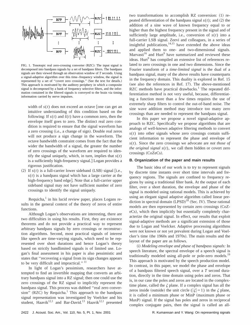
wherez is the corresponding complex-frequency variable.this case the frequency response of the system is the funcH(z) evaluated around the unit circleuzu51.23 The fre-quency response of the discrete time system is 2p periodic.In the above cases the frequency is regarded as a comvariable. Analogously, we could also regardtime as a com-plex variableand thereby define a complex-time~t! plane,wheret,s1 j t . In thet plane, we may model a nonperiodcomplex-valued signal as

x~t!5c2

)k51Q ~t2zk!

)k51P ~t2pk!

~1!

given sufficient number of polespk and zeroszk .Analogous to the frequency responseH( j v), the signal

x(t) is obtained by evaluatingx(t) along thejt axis. Carry-ing the above analogy further, the dual of a complefrequencyz plane, is a complex-timez plane, suitable formodeling complex-valued periodic signals. In this casesignal function in terms of poles and zeros is

x~z!5c3

)k51Q ~z2zk!

)k51P ~z2pk!

. ~2!

We obtain the periodic signalx(t) by evaluatingx(z) aroundthe unit circleuzu51, i.e.,z5e2 j Vt, whereV52p/T is thefundamental frequency andT is the period. Hence, the uncircle in thez plane corresponds to the time interval 0 toTseconds. Figure 2 shows typical pole/zero plots in the tcomplex-time planes. From the location of poles and zerothe z plane, we can generally infer where in time~0 to Tseconds! the peaks and troughs in the envelope ofx(t) arelocated. Voelcker24 called this way of modeling signals as‘‘product representation of signals.’’ Also refer to recework by Poletti,25 Picinbono,26 and Kumaresan.18

Further, the concept of causality in the systems dom~i.e., the impulse response of a causal system is zeronegative time! is the dual of analyticity in the signal domai@i.e., the spectrum of an analytic signalx(t) is zero for nega-tive frequency#. Also, the group delay~the negative of thederivative of the phase response of a system with respefrequency! is the dual of instantaneous frequency~IF! ~thetime derivative of the phase! of x(t). In the next section weshall consider periodic and analytic signal models thatanalogs of finite impulse response~FIR! systems. Real-valued signals are dealt with in a later section.

A. FIR-like signal models in the z plane

Consider a periodic analytic signalsa(t), with periodTseconds. LetV52p/T denote its fundamental angular frequency. Ifsa(t) has a finite bandwidth, it may be describeby the following model for a sufficiently largeM, over aninterval of T seconds:

sa~ t !5ej v l t(k50

M

akejkVt, ~3!

2423R. Kumaresan and Y. Wang: On representing signals

FIG. 2. Poles and zeros in complex-time planes: Thet plane is suitable for modeling nonperiodic signals and thez plane for modeling periodic signals.

thu

f

ivec-

-ec-

ntteul

nee

f tin

eg-

--

rP or

.

eni-

thatdr,

ideosin-e

wherev l>0, which represents a frequency translation, islow-frequency band edge, that we take to be an integer mtiple of V, sayv l5KV. ak are the complex amplitudes othe sinusoidsejkVt;a0 ,aMÞ0. By analytic continuation wemay regardsa(t) as the functionsa(z)5z2K(a01a1z21

1a2z221¯aMz2M) evaluated around the unit circle,z5e2 j Vt. In sa(z) we use the negative powers ofz in order tomaintain the analogy with the traditional use of negatpowers ofz in the complex-frequency domain. We may fator this polynomial into itsM (5P1Q) factors and rewritesa(t) as

~4!

wherep1 ,p2 ,...,pP , andq1 ,q2 ,...,qQ denote the polynomi-al’s roots; pi5upi uej u i, qi5uqi uej f i and upi u,1 and uqi u.1. Thus,pi ’s denote roots inside the unit circle in the complex plane, andqi are outside the unit circle. Currently wassume that there are no roots on the unit circle. Each faof the form (12pie

j Vt) in the above is called an ‘‘elementary signal.’’24 The pi and qi are referred to as~nontrivial!zeros of the signalsa(t). The above expressions, represeing a bandlimited periodic signal, are, of course, the counpart of the frequency responses of the standard finite impresponse~FIR! filters.27

The factors corresponding to the zeros inside the ucircle, ) i 51

P (12piej Vt), constitute the minimum phas

~MinP! signal. Similarly the factors corresponding to the zros outside the circle,ej v l t) i 51

Q (12qiej Vt), constitute the

~frequency translated! maximum phase~MaxP! signal. Theseare the direct counterparts of the frequency responses owell-known minimum and maximum phase FIR filtersdiscrete-time systems theory.23 Just as in systems theory~seeSec. 10.3 in Ref. 23! the phase of the MinP signal is thHilbert transform of its log envelope. That is, the MinP sinal may be expressed in the formea(t)1 j a(t), wherea(t) is

2424 J. Acoust. Soc. Am., Vol. 110, No. 5, Pt. 1, Nov. 2001

el-

tor

-r-se

it

-

he

the Hilbert transform ofa(t). See Ref. 18 for details. Similarly, since a maximum phase~MaxP! signal has zeros out

side the unit circle, it may be expressed aseb(t)2 j b(t), whereb(t) is the Hilbert transform ofb(t). Thus, the envelope ophase alone is sufficient to essentially characterize a Mina MaxP signal. Along the same lines, an all-phase~AllP!analytic signal~the analog of an all-pass filter! would be ofthe formej c(t). Thus,sa(t) may be expressed as

~5!

Ac is a0 ) i 51Q (2qi). The formulas fora(t) andb(t) depend

on the particular values ofpi andqi , respectively. See Ref18 for details.

Just as the MixP systems~with zeros inside and outsidthe unit circle! may be decomposed into all-pass and mimum phase systems~see Sec. 5.6 in Ref. 23!, so toosa(t)may be decomposed into two component signals. Notein Eq. ~4! the zeros,qi andpi are assumed to be outside aninside the unit circle, respectively. To obtain the AllP factowe shall reflect theqi to inside the circle~as 1/qi* ! and can-cel them using poles. Then we may group all the zeros insthe unit circle to form a different MinP signal and the zeroutside the circle and the poles that are their reflectionsside the unit circle to form the all-phase or AllP part of thsignal. That is,

~6!

R. Kumaresan and Y. Wang: On representing signals

elnt

as

uoo

an

igru

lth

e

hili

n

s5.5

f

Equivalently, multiplying and dividing Eq.~5! by ej 2b(t) andcollecting terms, we get

~7!

This grouping of signals is, of course, analogous to the wknown decomposition of a linear discrete-time system iminimum phase and all-pass systems~Sec. 5.6 in Ref. 23!.Analogous to the fact that the group delay of the all-pfilters is always positive~Sec. 5.5 in Ref. 23!, the instanta-neous frequency~IF! of the AllP part will always bepositive18 ~even if v l , the lower band edge, is zero!. Hencewe18 called the IF of the AllP part the positive instantaneofrequency or PIF. Later in this paper we use the above mels to represent the envelopes and phases of successivelapping segments of a signal. A real bandpass signals(t) ismodeled as the real part ofsa(t). For a slowly varying signalone can imagine that thepi andqi are slowly drifting param-eters that characterize the signal’s envelope and phase vtions. We wish to capture in certain zero-crossing locatiothe behavior of the slowly varying parameterspi andqi .

III. ZERO CROSSINGS THAT CHARACTERIZEANALYTIC BANDPASS SIGNALS

In this section we show that the real~or imaginary! partof analytic bandpass signals~i.e., the MinP, MaxP, and AllPsignals! we introduced in the previous section are RZ snals, i.e., their zero crossings are sufficient to reconstthese signals.

A. Zero crossings related to minimum Õmaximumphase signals

Consider a MinP signal,hm(t), defined as follows:

hm~ t !5h01h1ej Vt1h2ej 2Vt1¯1hmejmVt. ~8!

An analytic continuation ofhm(t) in the z plane is denotedby Hm(z),

Hm~z!5h01h1z211h2z221¯1hmz2m. ~9!

Sincehm(t) is MinP, the roots ofHm(z) lie strictly inside theunit circle. LetHm* (1/z* ) denote the reciprocal polynomia~with roots in reciprocal conjugate locations, i.e., outsideunit circle!:

Hm* ~1/z* !,h0* 1h1* z11h2* z21¯1hm* zm. ~10!

We define two other polynomials usingHm(z) andHm* (1/z* ):

P~z!5zp/2Hm~z!1z2p/2Hm* ~1/z* !, ~11!

Q~z!5zp/2Hm~z!2z2p/2Hm* ~1/z* !. ~12!

Note that the coefficients ofP(z) and Q(z) haveconjugate-even and conjugate-odd symmetry, respectivWe now show that ifp>m, all the roots ofP(z) andQ(z)are on the unit circle and interlaced with each other. Tresult is a direct analog of results known in the speecherature as ‘‘line spectrum frequencies.’’20,21

J. Acoust. Soc. Am., Vol. 110, No. 5, Pt. 1, Nov. 2001

l-o

s

sd-ver-

ria-s

-ct

e

ly.

st-

Rewriting Eqs.~11! and~12! in a product form, we have

P~z!5zp/2Hm~z!@11G~z!#, ~13!

Q~z!5zp/2Hm~z!@12G~z!#, ~14!

whereinG(z) is an all-pass or all-phase function,

G~z!,z2pHm* ~1/z* !

Hm~z!. ~15!

G(z) can be factored as

G~z!5ej ~Vt01mp!z2~p2m!)i 51

mz i* 2z21

12z iz21 , ~16!

where z i ’s are the roots ofHm(z). z i5r iej Vt i, and r i,1.

Vt05/(h0* /h0). SinceG(z) is an all-pass function, we cawrite

G~z!uz5e2 j Vt5ej c~ t !. ~17!

It should be clear from Eqs.~13! and ~14! that P(z) andQ(z) have roots at the locations whereej c(t) equals21 and1, respectively.

The phase functionc(t) can further be expressed afollows ~similar to the phase of all-pass filters as in Sec.in Ref. 23!:

c~ t !5Vt01mp1~p2m!Vt

1(i 51

m

2 tan21S r i sin@V~ t1t i !#

12r i cos@V~ t1t i !#D . ~18!

The instantaneous frequency,f (t), of G(e2 j Vt) is (1/2p)3@dc(t)/dt# and is given by

f ~ t !5v

2p S ~p2m!1(i 51

m 12r i2

u12r iej @V~ t1t i !#u2D . ~19!

If p>m, and since allr i,1, we conclude thatf (t).0, i.e.,f (t) is a PIF. Thereforec(t) is a monotonically increasingfunction. Letf0 denote the phase ofG(e2 j Vt) at t50, i.e.,c(0)5f0 , and c(2p/V)5f012pp. Therefore, c(t)crosses lines corresponding to each integer multiple op@odd and even multiples ofp for P(z) and Q(z), respec-tively# exactly once, resulting in 2p crossing points for 0<Vt,2p. Because the solution toP(z)50 or Q(z)50requires thatG(z)561, these points constitute the total 2proots ofP(z) andQ(z) alternately on the unit circle.20,21

SinceHm(z) is MinP, the phase ofHm(z) ~when evalu-ated around the unit circleuzu51! and its log envelope arerelated by the Hilbert transform.18,23 That is,

Hm~z!uz5e2 j Vt5eg~ t !1 j g~ t !, ~20!

where the phase functiong(t) is the Hilbert transform of thelog-magnitude function g(t). Similarly, evaluatingHm* (1/z* ) around the unit circle we have

Hm* ~1/z* !uz5e2 j Vt5eg~ t !2 j g~ t !. ~21!

Plugging Eq.~20!, Eq.~21! andz5e2 j Vt in Eq. ~11! and Eq.~12!, we have

p~ t !5P~ej Vt!52eg~ t ! cosS p

2Vt2g~ t ! D . ~22!

2425R. Kumaresan and Y. Wang: On representing signals

ng

s1

-as

siy

P

,

on

e

n-

n-r an

s

f 1f

c-

tion

nal

Similarly,

q~ t !5 jQ~ej Vt!52eg~ t ! sinS p

2Vt2g~ t ! D . ~23!

Sinceeg(t) has no real zero crossings, all real zero crossiof p(t) andq(t) are due to the cosine and the sine term.

Given the zero-crossing locationst1 ,t2 ,...,tp corre-sponding to p(t), we can compute the rootej Vt1,ej Vt2,...,ej Vtp. Then the product of the factors (2ej Vt iz21), i 51,2,...,p gives P(z) ~up to a scale factor!.Similarly, one obtainsQ(z) from the zero crossings ofq(t).Using P(z) andQ(z) @in Eqs.~11! and~12!#, we can deter-mine Hm(z) and hencehm(t). Thus, only zero-crossing information is sufficient to reconstruct signals that are the re(or imaginary) part of frequency translated MinP signals. Amentioned before, such signals are called real zero (RZ)nals. If the given hm(t) is a MaxP signal, we can simplinterchange the roles ofHm(z) and Hm* (1/z* ) in the previ-ous discussion, and all the above results are still valid.

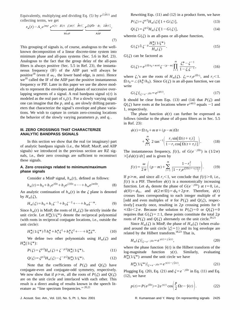
A simple example is shown in Fig. 3. We picked a Minsignalhm(t) with

Hm~z!51.01~0.69312 j 1.7071!z211~21.2025

2 j 0.7020!z221~20.23171 j 0.4913!z23

1~0.14361 j 0.0461!z241~0.0002

2 j 0.0290!z251~20.00562 j 0.0003!z26

1~0.00021 j 0.0007!z27,

wherem57. P(z) andQ(z) were calculated from Eq.~11!and Eq.~12!, wherep58. Their corresponding RZ signalsp(t) andq(t), are plotted in Figs. 3~a! and 3~b!. The roots/zeros ofP(z) and Q(z) are shown in Figs. 3~c! and 3~d!,respectively. Note thatP(z) andQ(z) have all their zeros onthe unit circle and they are interlaced. Note also the relati

FIG. 3. Real-zero~RZ! signals related to MinP signals: Thep(t) andq(t)calculated from a minimum phase signalhm(t) are plotted in~a! and ~b!.The roots/zeros of correspondingP(z) and Q(z) with p58.m are dis-played in~c! and ~d!.

2426 J. Acoust. Soc. Am., Vol. 110, No. 5, Pt. 1, Nov. 2001

s

l

g-

-

ship between the roots ofP(z) andQ(z) in thez plane withthe zero crossings ofp(t) andq(t).

B. Zero crossings related to all-phase signals

All-phase ~AllP! signals are analytic signals that havboth poles and zeros. If the poles are inside the unit circle@asin E(e2 j Vt) below#, then the spectrum of the signal is cofined to the positive side of the frequency axis~analogous tocausal IIR filters!. If the poles are outside the unit circle@asin F(e2 j Vt) below#, then the spectrum of the signal is cofined to the negative side of the frequency axis. Consideall-phase~AllP! signalE(e2 j Vt) defined as follows:

E~e2 j Vt!51

u) i 51Q ~2qi !u

) i 51Q ~12qie

j Vt!

)i 51

Q S 121

qi*ej VtD . ~24!

As before, by analytic continuation we can writeE(z) asfollows:

E~z!5ej f1z2QB~z!

B* ~1/z* !, ~25!

whereB(z),) i 51Q (12qi

21z). One may verify Eq.~24! bysubstitutingz5e2 j Vt in Eq. ~25!. The roots ofB(z) areqi ,i 51,2,...,Q, with 1/qi* 5r ie

j Vt i, and r i,1. Since all theroots of B(z) fall outside the unit circle,B(z) is a MaxPsignal and theB* (1/z* ) is a MinP signal. Clearly,E(z) isalready in the form ofG(z) encountered in the previousection. Hence, the instantaneous frequency ofE(e2 j Vt) isalways positive and the phase function ofE(e2 j Vt) is amonotonically increasing function. Therefore the zeros o1E(z) and 12E(z) have properties identical to those opolynomialsP(z) and Q(z) discussed in the previous setion. That is, 11E(z) and 12E(z) each haveQ zeros on theunit circle and they are interlaced. Further, using the notain Eqs.~6! and ~7! we can writeE(e2 j Vt) as follows:

E~e2 j Vt!5ej @QVt1f122b~ t !#. ~26!

Thus the unit magnitude root locations of 16E(z) corre-spond to zero crossings of the waveform 16cos@QVt1f1

22b(t)# or the waveform sin@QVt1f122b(t)#. We shall de-fine the imaginary part ofE(e2 j Vt) ase3(t):

e3~ t !5sin@QVt1f122b~ t !#. ~27!

Given the zero-crossing locationst1 ,t2 ,...,t2Q correspond-ing to sin@QVt1f122b(t)# or 16cos@QVt1f122b(t)#, wecan compute the rootsej Vt1,ej Vt2,...,ej Vt2Q. Then we shalldefinePB(z)5) i(12ej Vt iz21), where the set$i% consists ofodd integers 1,3,5,...,2Q21. Similarly, we shall defineQB(z)5) i(12ej Vt iz21), where the set$i% consists of evenintegers 2,4,6,...,2Q. Using PB(z) and QB(z) @similar toEqs.~11! and~12!#, we can determineB(z) and henceE(z)to within a scale factor.Thus, the zero-crossing informatioof e3(t) alone is sufficient to reconstruct the AllP signE(e2 j Vt) up to a complex scale factor. Hencee3(t) is a RZsignal.

Similarly, we may consider

R. Kumaresan and Y. Wang: On representing signals

.id

g

-

erthgiigrein

P

re

th

neCo

ixhe

in

a-onl/

eC

fe

ini-,

al-

ur

nyre

e

plex

-a

s by

F~e2 j Vt!5U)i 51

P

~2pi* !U ) i 51P ~12pie

j Vt!

)i 51

P S 121

pi*ej VtD . ~28!

The zeros ofF(e2 j Vt) arepi , i 51,2,...,P. pi5giej Vt i, and

gi,1. The poles ofF(e2 j Vt) are outside the unit circleThusF(e2 j Vt) has a spectrum confined to the negative sof the frequency axis and its IF is always negative~NIF!. Asbefore, 11F(e2 j Vt) and 12F(e2 j Vt) each haveP zeros onthe unit circle that are interlaced. Again, if the zero crossinof e4(t),

e4~ t !5sin@PVt1f222a~ t !#, ~29!

are known, then we can reconstruct~using the same algorithm described above! the AllP signalF(e2 j Vt) to within ascale factor. We will make use ofe3(t) and e4(t) in Sec.V B.

In summary, in this section we have shown that the zcrossings of certain special functions implicitly representunderlying analytic signals. In other words, the real or imanary parts of the MinP, MaxP, and AllP signals, are RZ snals, since they are essentially characterized by theirzero crossings. In general, analytic signals are neither MMaxP nor AllP, but mixed-phase~MixP! signals. Hence wehave to first decompose an arbitrary MixP signal into MinMaxP and AllP signals as shown in Eqs.~6! and ~7!. Anelegant algorithm for achieving this decomposition is psented next. In Sec. V we consider real-valued signals.

IV. SEPARATING THE MINP AND ALLP PARTS OF ANANALYTIC BANDPASS SIGNAL USING LPSD

In this section we present a simple algorithm calledlinear prediction in the spectral domain~LPSD!.18 The de-tails of the LPSD algorithm, which separates the MinP aAllP components of a MixP signal, were presented in R18. Here we summarize these results for completeness.sider the MixP signal in Eq.~3! or Eq. ~4!:

sa~ t !5ej v l t(k50

M

akejkVt ~30!

5a0ej v l t)i 51

P

~12piej Vt!)

i 51

Q

~12qiej Vt!. ~31!

Using the notation in Sec. II, we may expresssa(t) as

sa~ t !5uAcue@a~ t !1b~ t !#ej ~~v l1QV!t1a~ t !2b~ t !1f1!. ~32!

Note thatAce@a(t)1b(t)# is the envelope ofsa(t). The LPSD

algorithm separates the MinP and AllP components of Msignal. This decomposition is achieved by minimizing tenergy in an error signale(t) that is defined ase(t)5hm(t)sa(t). The energy ine(t) is defined as follows:

E0

T

ue~ t !u2 dt5E0

T

usa~ t !hm~ t !u2 dt. ~33!

hm(t) is synthesized using the following formula:

hm~ t !5h01h1ej Vt1h2ej 2Vt1¯1hmejmVt, ~34!

J. Acoust. Soc. Am., Vol. 110, No. 5, Pt. 1, Nov. 2001

e

s

oe--alP/

/

-

e

df.n-

P

whereV52p/T. Note thathm(t) is identical to that definedin Sec. III A. The LPSD algorithm minimizes the energythe error signale(t) @the integral in Eq.~33! is replaced by adiscrete approximation# by choosing the coefficientshl ,whereh0 is constrained to be 1. Thus, the above minimiztion problem is the direct analog of the autocorrelatimethod of the linear prediction well-known in spectraspeech analysis28 as LPC or all-pole modeling or inversfiltering. hm(t) is the analog of the inverse filter used in LPand hence is called the ‘‘inverse signal.’’18 The LPSD algo-rithm finds an inverse signalhm(t) such that the envelope othe error signale(t) is flattened. This can be achieved if thorder m of hm(t) is sufficiently high.m has to be large ifthere are deep nulls in the signal envelope. After the mmization, since the error signale(t) has a constant envelope

hm~ t !'e2@a~ t !1b~ t !#e2 j @a~ t !1b~ t !#. ~35!

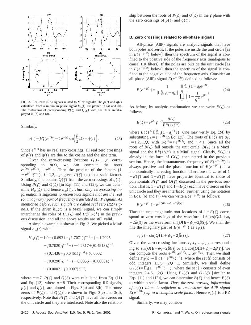
Figure 4 gives an illustrative example. An analytic signsa(t) was synthesized from Eq.~3! using seven Fourier coefficients (M56): a051, a1520.602423.2827i , a2

525.644111.5835i , a3520.145417.4390i , a456.482221.1832i , a5524.630626.7388i , a651.073712.7369i .The real part ofsa(t) is plotted in Fig. 4~a!. The analyticsignal sa(t) has two zeros inside the unit circle and fooutside, as shown in Fig. 4~b!. Note thathm(t) computedusing the LPSD algorithm is always a MinP signal for aorderm, i.e., all of its zeros are inside the unit circle. Figu4~d! displays the roots ofHm(z). This result is well knownin spectral analysis literature.28 The estimated envelop

FIG. 4. Envelope of a MixP signal represented by zero crossings: A comsignal sa(t) is synthesized with six zeros~four outside the unit circle andtwo inside the unit circle!. The zeros ofsa(t) are plotted in~b!. The real partof sa(t) is plotted in ~a!. The roots ofHm(z) calculated using the LPSDalgorithm are shown in~d!. Note thatHm(z) is MinP. The estimated envelope 1/uhm(t)u is shown~solid line! in ~c!; the true envelope is shown bydotted line. In~e!, both RZ functionsp(t) and q(t) are plotted by a solidline and a dashed line, respectively. Since they are described fully~to withina scale factor! by their zero crossings, we can representp(t) and q(t) byonly marking their zero-crossing time locations. We show those locationspikes along the time axis in~e!. The roots ofP(z) andQ(z), all on the unitcircle, are displayed in~f!. The roots ofP(z) are denoted by a ‘‘s’’ andthose ofQ(z) are denoted by a ‘‘L.’’

2427R. Kumaresan and Y. Wang: On representing signals

,

fung

n-

.o

thto

in

izes

anintore-theac-pre-ith-a

ec-

uedf

and

theactboththe

e-al-

s

inds

henalsrsen-

1/uhm(t)u is shown~solid line! in Fig. 4~c!; the true envelopeusa(t)u, is also shown using a dotted line. In Fig. 4~e!, bothRZ functionsp(t) andq(t) @computed using Eqs.~11!, ~12!,~22!, and ~23! with p58.m# are plotted with a solid lineand a dashed line, respectively. Since they are described~to within a scale factor! by their zero crossings, we carepresentp(t) andq(t) by only marking their zero-crossintime locations. We show these locations in Fig. 4~e!, by atrain of ‘‘spikes’’ along the time axis. Note that we cauniquely reconstructhm(t) from these spike locations. Comparing the envelope in Fig. 4~c! and the spike train in Fig4~e!, note that when the envelope is large, the densityspikes@due to bothp(t) andq(t) together# around that timelocation is higher. The zeros ofP(z) ~denoted by a ‘‘s’’ !and Q(z) ~denoted by a ‘‘L’’ ! are displayed in Fig. 4~f!.From the above we conclude that the envelope part ofanalytic signalsa(t) has been successfully converted intwo RZ signals or two spike trains.

The error signale(t)5sa(t)hm(t) obtains the approxi-mation to the AllP part in Eq.~7!,

e~ t !'ej @~v l1QV!t1f122b~ t !#5ej c~ t !. ~36!

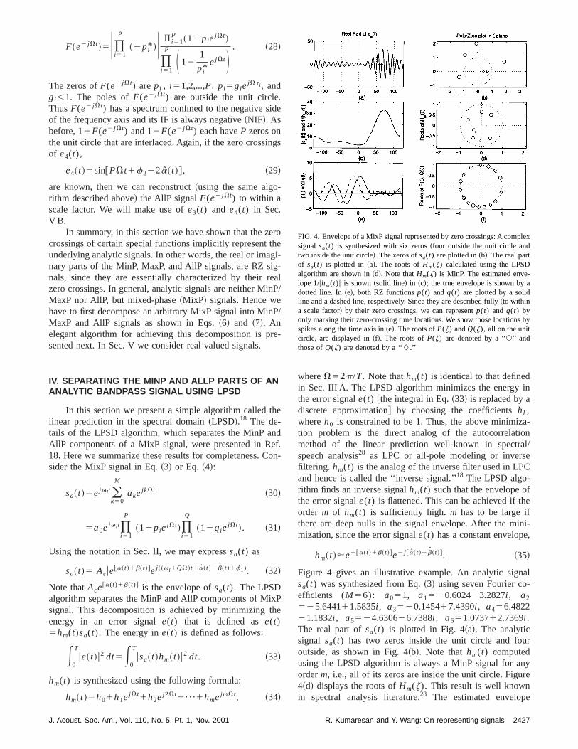
Note thate(t) is identical to the functionE(e2 j Vt) in Sec.III B, except for the frequency translation termej v l t. e(t)~with v l50! and its real and imaginary parts are shownFig. 5. The PIF ofe(t) is shown in Fig. 5~a!. The phase ofe(t), denoted byc(t), is plotted in Fig. 5~b!. Because the IFof e(t) is always positive, the phasec(t) is a monotonicallyincreasing function. The real part ofe(t) ~i.e., cos@(QV)t1f122b(t)#! and its imaginary part, sin@(QV)t1f122b(t)#are shown in Fig. 5~c! and Fig. 5~d!, respectively. As ex-plained in Sec. III B@between Eqs.~26! and ~27!# the alter-

FIG. 5. All-phase~AllP! signal represented by zero crossings: The IFs~i.e.,PIFs! of e(t) @both true~solid line! and estimated# are shown in~a!; thephase ofe(t), denoted byc(t), is plotted in~b!; because the instantaneoufrequency ofe(t) is positive, the phasec(t) ~with v l50! is a monotoni-cally increasing function. The real part and imaginary part ofe(t) are shownin ~c! and ~d!, respectively. The indicated spike locations are sufficientformation for reconstructing the AllP signal except for a scale factor anfrequency translation. Note that in~c! the spikes correspond to the locationwhen the real part ofe(t) equals61.

2428 J. Acoust. Soc. Am., Vol. 110, No. 5, Pt. 1, Nov. 2001

lly

f

e

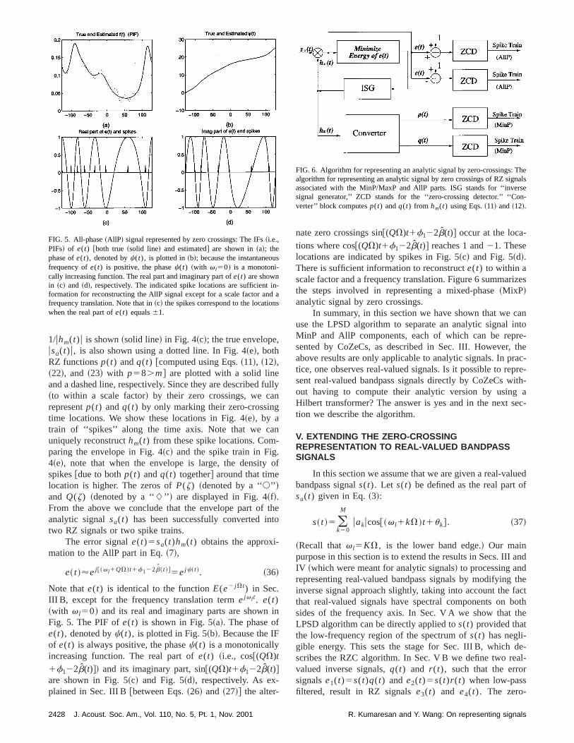
nate zero crossings sin@(QV)t1f122b(t)# occur at the loca-tions where cos@(QV)t1f122b(t)# reaches 1 and21. Theselocations are indicated by spikes in Fig. 5~c! and Fig. 5~d!.There is sufficient information to reconstructe(t) to within ascale factor and a frequency translation. Figure 6 summarthe steps involved in representing a mixed-phase~MixP!analytic signal by zero crossings.

In summary, in this section we have shown that we cuse the LPSD algorithm to separate an analytic signalMinP and AllP components, each of which can be repsented by CoZeCs, as described in Sec. III. However,above results are only applicable to analytic signals. In prtice, one observes real-valued signals. Is it possible to resent real-valued bandpass signals directly by CoZeCs wout having to compute their analytic version by usingHilbert transformer? The answer is yes and in the next stion we describe the algorithm.

V. EXTENDING THE ZERO-CROSSINGREPRESENTATION TO REAL-VALUED BANDPASSSIGNALS

In this section we assume that we are given a real-valbandpass signals(t). Let s(t) be defined as the real part osa(t) given in Eq.~3!:

s~ t !5 (k50

M

uakucos@~v l1kV!t1uk#. ~37!

~Recall thatv l5KV, is the lower band edge.! Our mainpurpose in this section is to extend the results in Secs. IIIIV ~which were meant for analytic signals! to processing andrepresenting real-valued bandpass signals by modifyinginverse signal approach slightly, taking into account the fthat real-valued signals have spectral components onsides of the frequency axis. In Sec. V A we show thatLPSD algorithm can be directly applied tos(t) provided thatthe low-frequency region of the spectrum ofs(t) has negli-gible energy. This sets the stage for Sec. III B, which dscribes the RZC algorithm. In Sec. V B we define two revalued inverse signals,q(t) and r (t), such that the errorsignalse1(t)5s(t)q(t) and e2(t)5s(t)r (t) when low-passfiltered, result in RZ signalse3(t) and e4(t). The zero-

-a

FIG. 6. Algorithm for representing an analytic signal by zero-crossings: Talgorithm for representing an analytic signal by zero crossings of RZ sigassociated with the MinP/MaxP and AllP parts. ISG stands for ‘‘invesignal generator,’’ ZCD stands for the ‘‘zero-crossing detector.’’ ‘‘Coverter’’ block computesp(t) andq(t) from hm(t) using Eqs.~11! and~12!.

R. Kumaresan and Y. Wang: On representing signals

-

st

:

can

chhushe

he

fn,

al

n

-w-ted

asi-lytic

tohanP

l-

roa

es

lop

crossing locations ofe3(t) ande4(t) are sufficient to recon-struct the MinP and MaxP parts ofsa(t) and hence characterizes(t).

A. Computing the inverse signal h m„t … from a realbandpass signal s „t …

Considers(t) over an interval of 0 toT seconds. Weshall rewrites(t) for convenience as follows:

s~ t !5 (k52N

N

bkejkVt. ~38!

Since s(t) is real-valued,b2k5bk* . Comparing Eqs.~37!and ~38!, we note thatbK1 i5ai , for i 50,1,...,M . N5K1M . vh5NV is the higher band edge. Lets(t), be suchthat the Fourier coefficientsb2K11 ,...,b0 ,...,bK21 are equalto zero for someK,N. An example of the spectrum ishown in Fig. 7~a!. Following the development in Sec. IV, leus define an error signale(t) over 0 toT seconds as follows

e~ t !5s~ t !hm~ t !, ~39!

wherehm(t)511( l 51m hle

jl Vt. As before, our goal is to findan inverse signal,hm(t) ~i.e., choose the coefficients,hl!,such that the energy in the error signale(t) is minimized.Plugging in the expression fors(t) from Eq. ~38! into theerror-energy expression, we get

E0

T

ue~ t !u2 dt5E0

2

us~ t !hm~ t !u2 dt ~40!

5T (n52N

N1m

ugnu2, ~41!

where gn5bn* hn ~* denotes linear convolution!, and h0

51. The inverse signal coefficients,hl , can be determinedby solving linear equations using the LPSD algorithm.

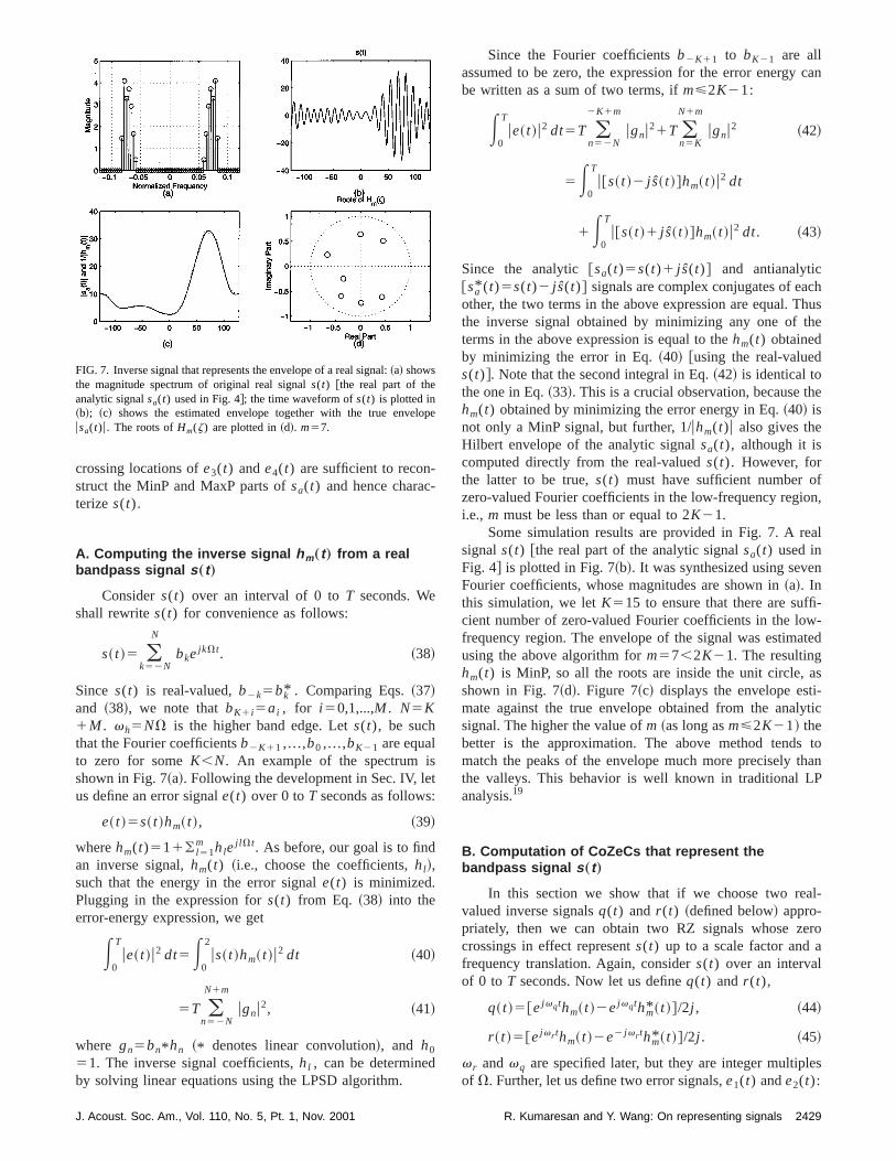
FIG. 7. Inverse signal that represents the envelope of a real signal:~a! showsthe magnitude spectrum of original real signals(t) @the real part of theanalytic signalsa(t) used in Fig. 4#; the time waveform ofs(t) is plotted in~b!; ~c! shows the estimated envelope together with the true enveusa(t)u. The roots ofHm(z) are plotted in~d!. m57.

J. Acoust. Soc. Am., Vol. 110, No. 5, Pt. 1, Nov. 2001

Since the Fourier coefficientsb2K11 to bK21 are allassumed to be zero, the expression for the error energybe written as a sum of two terms, ifm<2K21:

E0

T

ue~ t !u2 dt5T (n52N

2K1m

ugnu21T (n5K

N1m

ugnu2 ~42!

5E0

T

u@s~ t !2 j s~ t !#hm~ t !u2 dt

1E0

T

u@s~ t !1 j s~ t !#hm~ t !u2 dt. ~43!

Since the analytic@sa(t)5s(t)1 j s(t)# and antianalytic@sa* (t)5s(t)2 j s(t)# signals are complex conjugates of eaother, the two terms in the above expression are equal. Tthe inverse signal obtained by minimizing any one of tterms in the above expression is equal to thehm(t) obtainedby minimizing the error in Eq.~40! @using the real-valueds(t)#. Note that the second integral in Eq.~42! is identical tothe one in Eq.~33!. This is a crucial observation, because thm(t) obtained by minimizing the error energy in Eq.~40! isnot only a MinP signal, but further, 1/uhm(t)u also gives theHilbert envelope of the analytic signalsa(t), although it iscomputed directly from the real-valueds(t). However, forthe latter to be true,s(t) must have sufficient number ozero-valued Fourier coefficients in the low-frequency regioi.e., m must be less than or equal to 2K21.

Some simulation results are provided in Fig. 7. A resignals(t) @the real part of the analytic signalsa(t) used inFig. 4# is plotted in Fig. 7~b!. It was synthesized using seveFourier coefficients, whose magnitudes are shown in~a!. Inthis simulation, we letK515 to ensure that there are sufficient number of zero-valued Fourier coefficients in the lofrequency region. The envelope of the signal was estimausing the above algorithm form57,2K21. The resultinghm(t) is MinP, so all the roots are inside the unit circle,shown in Fig. 7~d!. Figure 7~c! displays the envelope estmate against the true envelope obtained from the anasignal. The higher the value ofm ~as long asm<2K21! thebetter is the approximation. The above method tendsmatch the peaks of the envelope much more precisely tthe valleys. This behavior is well known in traditional Lanalysis.19

B. Computation of CoZeCs that represent thebandpass signal s „t …

In this section we show that if we choose two reavalued inverse signalsq(t) and r (t) ~defined below! appro-priately, then we can obtain two RZ signals whose zecrossings in effect represents(t) up to a scale factor andfrequency translation. Again, considers(t) over an intervalof 0 to T seconds. Now let us defineq(t) and r (t),

q~ t !5@ej vqthm~ t !2ej vqthm* ~ t !#/2j , ~44!

r ~ t !5@ej vr thm~ t !2e2 j vr thm* ~ t !#/2j . ~45!

v r andvq are specified later, but they are integer multiplof V. Further, let us define two error signals,e1(t) ande2(t):

e

2429R. Kumaresan and Y. Wang: On representing signals

hf

l

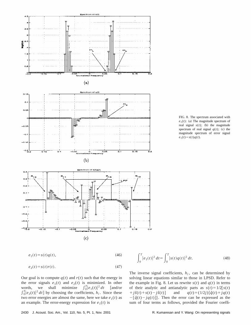
FIG. 8. The spectrum associated wite1(t): ~a! The magnitude spectrum oreal signal s(t); ~b! the magnitudespectrum of real signalq(t); ~c! themagnitude spectrum of error signae1(t)5s(t)q(t).

to

thefi-

e1~ t !5s~ t !q~ t !, ~46!

e2~ t !5s~ t !r ~ t !. ~47!

Our goal is to computeq(t) andr (t) such that the energy inthe error signalse1(t) and e2(t) is minimized. In otherwords, we shall minimize *0

Tue1(t)u2 dt @and/or*0

Tue2(t)u2 dt# by choosing the coefficients,hl . Since thesetwo error energies are almost the same, here we takee1(t) asan example. The error-energy expression fore1(t) is

2430 J. Acoust. Soc. Am., Vol. 110, No. 5, Pt. 1, Nov. 2001

E0

T

ue1~ t !u2 dt5E0

T

us~ t !q~ t !u2 dt. ~48!

The inverse signal coefficients,hl , can be determined bysolving linear equations similar to those in LPSD. Referthe example in Fig. 8. Let us rewrites(t) andq(t) in termsof their analytic and antianalytic parts ass(t)51/2@s(t)1 j s(t)1s(t)2 j s(t)# and q(t)5(1/2j )$q(t)1 jq(t)2@ q(t)2 jq(t)#%. Then the error can be expressed assum of four terms as follows, provided the Fourier coef

R. Kumaresan and Y. Wang: On representing signals

cients corresponding to each of the four kernels do not overlap:

~49!

~50!

outh

e

of

r-

yc

f

-

we

weo ared

e-

The spectrum associated with each of the kernelse11, e12,e13, ande14 is clearly marked in Fig. 8.@Here we have usedthe same real signals(t) shown in Fig. 7.# If this nonoverlapcondition is met, then, as in the previous section all the fterms in the above expression will be equal. In that caseinverse signal,hm(t), obtained by minimizing any one of thterms in the above expression is equal to theq(t) obtainedby minimizing the error in Eq.~48! @using the real-valueds(t) and q(t)#. This guarantees a MinPhm(t) and hence1/uq(t)1 jq(t)u gives an estimate of the Hilbert envelopethe analytic ~and the antianalytic! signal. An example isgiven in Fig. 8. The spectrum ofs(t) andq(t) are shown inFigs. 8~a! and ~b!, respectively. The spectrum ofs(t)q(t) isgiven in Fig. 8~c!.

The nonoverlap condition requires thatq(t) must have asuitable carrier frequencyvq . There are two possible ovelaps in the spectrum ofs(t)q(t), i.e., betweene11 ande14,and betweene14 ande12. To avoid overlap betweene11 ande14, vq should be such that,vq<v l . In order to be able todetermineq(t) uniquely from the coefficientshl and viceversa@see Eq.~44!#, vq should be greater than (m11)V. Toavoid overlap betweene14 ande12 ~or e11 ande13! we shouldchoosem, the order ofq(t), such thatmV,vq21/2(vh

2v l). In summary, we should choose (m11)V,vq<v l

and mV,vq21/2(vh2v l). Similar comments also applto r (t), which is a real-valued signal on the higher-frequenside ofs(t). ~See Fig. 9.! In this case,v r>vh to avoid theoverlap betweene21 and e24; and mV,2v l to avoid theoverlap betweene24 ande22.

The real signals(t) could also be written in terms oenvelope and phase as follows@see Eq.~32!#:

s~ t !5uAcue@a~ t !1b~ t !#cos@~KV1QV!t1a~ t !2b~ t !1f1#.~51!

The real signalsq(t) and r (t) calculated by the abovementioned process are

q~ t !52 imag$e2@a~ t !1b~ t !#e2 j @vqt1a~ t !1b~ t !#% ~52!

52e2@a~ t !1b~ t !# sin@KVt1a~ t !1b~ t !#, ~53!

r ~ t !52 imag$e2@a~ t !1b~ t !#ej @vr t2a~ t !2b~ t !#% ~54!

J. Acoust. Soc. Am., Vol. 110, No. 5, Pt. 1, Nov. 2001

re

y

52e2@a~ t !1b~ t !# sin@NVt2a~ t !2b~ t !#, ~55!

where we chosevq5KV andv r5NV. Then the two errorsignals are

e1~ t !52uAcusin@~2KV1QV!t12a~ t !1f1#

1uAcusin@QVt22b~ t !1f1#, ~56!

e2~ t !52uAcusin$@~K1N!V1QV#t12b~ t !1f1%

1uAcusin@P~Vt22a~ t !1f2#. ~57!

Low pass filtering thee1(t) and e2(t) with the cut-off fre-quencyKV @refer to Fig. 8~c! and Fig. 9~c!#, we have

e3~ t !5uAcusin@QVt22b~ t !1f1#, ~58!

e4~ t !5uAcusin@PVt22a~ t !1f2#. ~59!

These two signals are the same as in Eq.~27! and Eq.~29!,but for a scale factor. From the discussions in Sec. III B,know that bothe3(t) and e4(t) are RZ signals and theydetermine the corresponding AllP factors. Using these,can reconstruct the corresponding analytic signals up tcomplex scale factor and a frequency translation. The filteerror signalse3(t) ande4(t) together with their ‘‘true’’ val-ues are displayed in Figs. 10~a! and ~b!.

C. Summary of RZC algorithm

The steps involved in the RZC algorithm are listed blow and shown in Fig. 11.

Real Zero Conversion (RZC) Algorithm(Analysis)

Given: Real-valued bandpass signal s ( t ).

1. Calculate h m( t ) (i.e. the coefficientsof h m( t )) by applying LPSD algorithm toreal signal s ( t )2. Compute q( t ) and r ( t ) from h m( t ) usingEqs. 44 and 45.3. Compute e 1( t ) 5s ( t ) q ( t ), and e 2( t )5s ( t ) r ( t ).4. Low-pass filter e 1( t ) and e 2( t ) to pro-duce e 3( t ) and e 4( t ). Determine the zero-

2431R. Kumaresan and Y. Wang: On representing signals

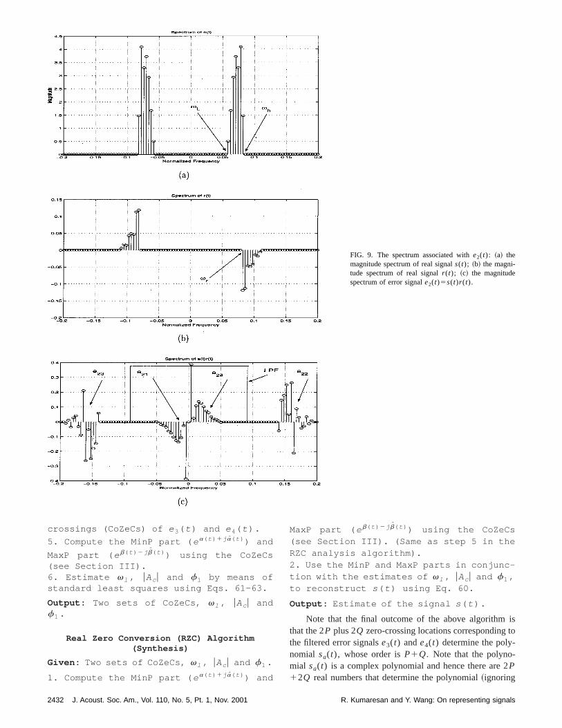
FIG. 9. The spectrum associated withe2(t): ~a! themagnitude spectrum of real signals(t); ~b! the magni-tude spectrum of real signalr (t); ~c! the magnitudespectrum of error signale2(t)5s(t)r (t).

isto

crossings (CoZeCs) of e 3( t ) and e 4( t ).

5. Compute the MinP part ( e a( t ) 1 j a( t ) ) and

MaxP part ( e b( t ) 2 j b( t ) ) using the CoZeCs(see Section III).6. Estimate v l , uAc u and f1 by means ofstandard least squares using Eqs. 61–63.

Output: Two sets of CoZeCs, v l , uAc u andf1 .

Real Zero Conversion (RZC) Algorithm(Synthesis)

Given: Two sets of CoZeCs, v l , uAc u and f1 .

1. Compute the MinP part ( e a( t ) 1 j a( t ) ) and

2432 J. Acoust. Soc. Am., Vol. 110, No. 5, Pt. 1, Nov. 2001

MaxP part ( e b( t ) 2 j b( t ) ) using the CoZeCs(see Section III). (Same as step 5 in theRZC analysis algorithm).2. Use the MinP and MaxP parts in conjunc-tion with the estimates of v l , uAc u and f1 ,to reconstruct s ( t ) using Eq. 60.

Output: Estimate of the signal s ( t ).

Note that the final outcome of the above algorithmthat the 2P plus 2Q zero-crossing locations correspondingthe filtered error signalse3(t) ande4(t) determine the poly-nomial sa(t), whose order isP1Q. Note that the polyno-mial sa(t) is a complex polynomial and hence there are 2P12Q real numbers that determine the polynomial~ignoring

R. Kumaresan and Y. Wang: On representing signals

rhehe

e

hekthrs

naibir

theeino

theis

wethe

innk,the

ruc-a

nce

l is1del

l-theofb/

lter

ghsws

r

areare

the first coef ficient a0 that is absorbed in the scale factoAc). Hence the RZC algorithm is a way of transforming tP1Q complex Fourier coefficients corresponding to ttrigonometric polynomial that represents s(t) into 2(P1Q) zero-crossing locations that implicitly determine thunderlying analytic signal sa(t).

We wish to make clear the conditions under which tabove transformation can be achieved. Recall that theidea in Sec. IV is to flatten the signal envelope by usingall-pole model~LPSD algorithm! thereby turning the errosignal e(t) into an AllP signal. The desirable properties asociated with the zero crossings ensue from this AllP sigThere are two situations under which it may not be possto completely flatten the envelope of a bandpass signal. Fif s(t) is such that its envelope dips to zero for somet @i.e.,sa(t) has one or more zeros on the unit circle#, then, clearlythe LPSD algorithm would require an extremely largem tofit an all-pole model to the signal envelope and hencenonoverlap conditions mentioned above may not be mSecond, ifs(t) is such that the Fourier coefficients in thlow-frequency region are not sufficiently small, then agathe above nonoverlap conditions are not met. These two c

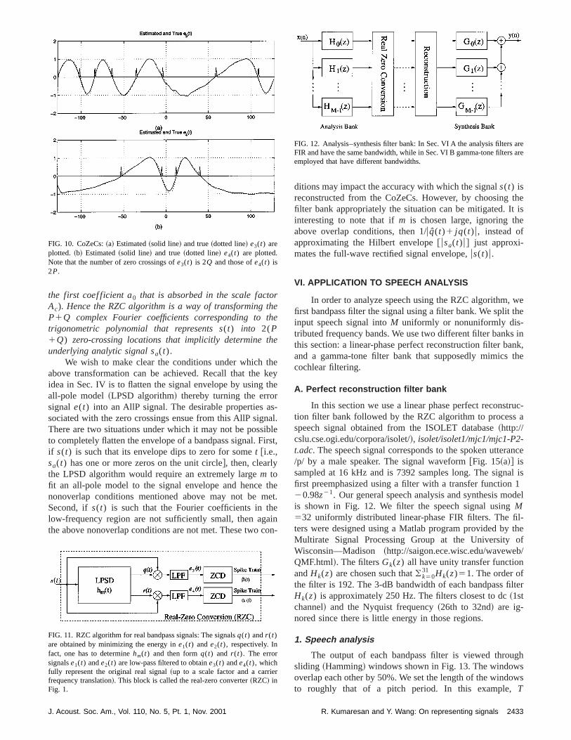
FIG. 10. CoZeCs:~a! Estimated~solid line! and true~dotted line! e3(t) areplotted. ~b! Estimated~solid line! and true~dotted line! e4(t) are plotted.Note that the number of zero crossings ofe3(t) is 2Q and those ofe4(t) is2P.

FIG. 11. RZC algorithm for real bandpass signals: The signalsq(t) andr (t)are obtained by minimizing the energy ine1(t) ande2(t), respectively. Infact, one has to determinehm(t) and then formq(t) and r (t). The errorsignalse1(t) ande2(t) are low-pass filtered to obtaine3(t) ande4(t), whichfully represent the original real signal~up to a scale factor and a carriefrequency translation!. This block is called the real-zero converter~RZC! inFig. 1.

J. Acoust. Soc. Am., Vol. 110, No. 5, Pt. 1, Nov. 2001

eye

-l.

lest,

et.

n-

ditions may impact the accuracy with which the signals(t) isreconstructed from the CoZeCs. However, by choosingfilter bank appropriately the situation can be mitigated. Itinteresting to note that ifm is chosen large, ignoring theabove overlap conditions, then 1/uq(t)1 jq(t)u, instead ofapproximating the Hilbert envelope@ usa(t)u# just approxi-mates the full-wave rectified signal envelope,us(t)u.

VI. APPLICATION TO SPEECH ANALYSIS

In order to analyze speech using the RZC algorithm,first bandpass filter the signal using a filter bank. We splitinput speech signal intoM uniformly or nonuniformly dis-tributed frequency bands. We use two different filter banksthis section: a linear-phase perfect reconstruction filter baand a gamma-tone filter bank that supposedly mimicscochlear filtering.

A. Perfect reconstruction filter bank

In this section we use a linear phase perfect reconsttion filter bank followed by the RZC algorithm to processspeech signal obtained from the ISOLET database~http://cslu.cse.ogi.edu/corpora/isolet/!, isolet/isolet1/mjc1/mjc1-P2-t.adc. The speech signal corresponds to the spoken uttera/p/ by a male speaker. The signal waveform@Fig. 15~a!# issampled at 16 kHz and is 7392 samples long. The signafirst preemphasized using a filter with a transfer function20.98z21. Our general speech analysis and synthesis mois shown in Fig. 12. We filter the speech signal usingM532 uniformly distributed linear-phase FIR filters. The fiters were designed using a Matlab program provided byMultirate Signal Processing Group at the UniversityWisconsin—Madison ~http://saigon.ece.wisc.edu/waveweQMF.html!. The filtersGk(z) all have unity transfer functionandHk(z) are chosen such that(k50

31 Hk(z)51. The order ofthe filter is 192. The 3-dB bandwidth of each bandpass fiHk(z) is approximately 250 Hz. The filters closest to dc~1stchannel! and the Nyquist frequency~26th to 32nd! are ig-nored since there is little energy in those regions.

1. Speech analysis

The output of each bandpass filter is viewed throusliding ~Hamming! windows shown in Fig. 13. The windowoverlap each other by 50%. We set the length of the windoto roughly that of a pitch period. In this example,T

FIG. 12. Analysis–synthesis filter bank: In Sec. VI A the analysis filtersFIR and have the same bandwidth, while in Sec. VI B gamma-tone filtersemployed that have different bandwidths.

2433R. Kumaresan and Y. Wang: On representing signals

hethmrieth

d-

toeo

e

ntd

-

-

s of

to--

r-to-

m-out-

op1sto-tert anr-he

ZC

w thectedis

d inanelon-belterwe

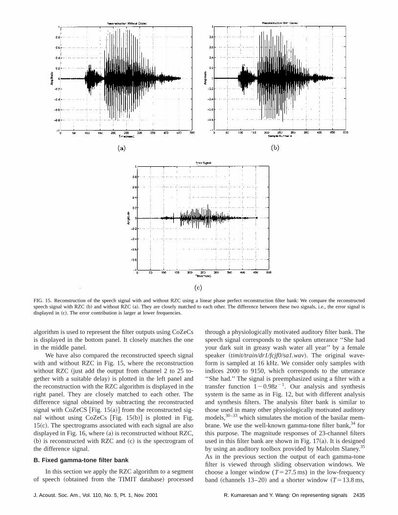
56.9 ms, except in the lower-frequency channels~channel 6and lower!, whereT513.8 ms~' twice the pitch period!.

Note that the spectrum of the windowed signal is tconvolution of the spectrum of the speech signal andspectrum of the window function. Hence, using the Haming window tends to reduce the magnitude of the Foucoefficients in the low-frequency region as required forRZC algorithm~see Sec. V B!.

We estimate the lower band edgev l and the higher bandedgevh of s(t) from the cut-off frequencies of each banpass filter. Then we setvq5v l2dV and v r5vh1dV,whered>0. d is a ‘‘guard’’ band and in this simulationd51. The orderm of hm(t) is chosen to be 7 in channels 26 and 9 in channels 7 to 25. To each block of the windowsignal in each channel, we apply the RZC algorithm. Feach block we obtaine3(t) ande4(t) as in Eq.~27! and Eq.~29! and determine their zero crossings~CoZeCs!. Usingthese zero crossings we estimate the MinP (ea(t)1 j a(t)) and

MaxP (eb(t)2 j b(t)) components. Note that the model of threal signal is

s~ t !5uAcue@a~ t !1b~ t !# cos@~v l1QV!t1a~ t !2b~ t !1f1#.~60!

After we have the estimates of MinP and MaxP componethe estimates ofv l , uAcu, andf1 are obtained by standarleast squares~see, for example, pp. 261–269 in Ref. 29!. Theleast squares estimate ofv l is obtained by finding the maximum of the function

4

T U E2T/2

T/2

s~ t !e2@a~ t !1b~ t !#e2 j @v l t1QVt1a~ t !2b~ t !# dtU2

.

~61!

MagnitudeuAcu, and the phasef1 can be shown to be approximatelyAc5Aa1

21a22 andf15arctan(2a2 /a1), where

FIG. 13. One segment of filtered speech with overlapped sliding windoWe used a Hamming window~6.9 ms duration!. Each window overlaps theprevious one by 50%.

2434 J. Acoust. Soc. Am., Vol. 110, No. 5, Pt. 1, Nov. 2001

e-r

e

dr

s,

a152

T E2T/2

T/2

s~ t !e2@a~ t !1b~ t !# cos$2@v l t1QVt1a~ t !

2b~ t !#%dt, ~62!

a252

T E2T/2

T/2

s~ t !e2@a~ t !1b~ t !# sin$2@v l t1QVt1a~ t !

2b~ t !#%dt. ~63!

Thus, each channel outputs the zero-crossing locatione3(t) ande4(t) and estimates ofAc , v l , andf1 .

2. Synthesis

Using the two sets of zero crossings, we reconstruca,b, a, b, and the corresponding MinP and MaxP compnents.~See the details in Sec. III B.! These are then combined with the estimatesv l , uAcu, andf1 , to reconstruct thewindowed signal as in Eq.~60!. Because each window ovelaps the other by 50%, adding the reconstructed blocksgether gives the reconstructed signal for each channel.

The first example simply uses an impulse input to deonstrate the analysis/synthesis idea. Figure 14 shows theputs of the filter bank when an impulse is input. In the tpanel we just plot the input impulse that is applied at the 8sample. The output of the filter bank without any RZC prcessing is shown in the middle panel. Although the filbank has perfect reconstruction property, the output is noimpulse ~but close! because we have included in the filtebank only filters numbered 2 to 25 as mentioned before. Tgroup delay of the filters@the cascade ofHk(z) andGk(z)# is96 samples. The reconstruction of the impulse when the R

s:FIG. 14. Reconstruction of an impulse with and without RZC usinglinear phase perfect reconstruction filter bank: We compare the reconstruimpulse with and without RZC, where the reconstruction without RZCplotted in the middle panel and the reconstruction with RZC is displayethe bottom panel. They are closely matched to each other. The top pshows the input impulse location. Since the filter bank is a perfect recstruction variety, we know that if the input is an impulse the output mustan impulse with a delay. The delay is equal to the group delay of the fi~96 samples!. However, the output is not exactly an impulse becauseomit the filters 1 and 26 to 32 from our filter bank.

R. Kumaresan and Y. Wang: On representing signals

onstructeignal is

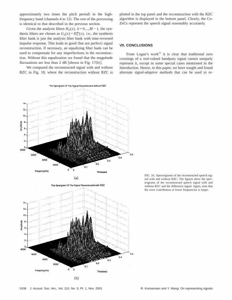
FIG. 15. Reconstruction of the speech signal with and without RZC using a linear phase perfect reconstruction filter bank: We compare the recdspeech signal with RZC~b! and without RZC~a!. They are closely matched to each other. The difference between these two signals, i.e., the error sdisplayed in~c!. The error contribution is larger at lower frequencies.

eCon

igono-

heThte-

a,f

en

ehadle

ithnce

assisto

ory-

lters

.onee

algorithm is used to represent the filter outputs using CoZis displayed in the bottom panel. It closely matches thein the middle panel.

We have also compared the reconstructed speech swith and without RZC in Fig. 15, where the reconstructiwithout RZC ~just add the output from channel 2 to 25 tgether with a suitable delay! is plotted in the left panel andthe reconstruction with the RZC algorithm is displayed in tright panel. They are closely matched to each other.difference signal obtained by subtracting the reconstrucsignal with CoZeCS@Fig. 15~a!# from the reconstructed signal without using CoZeCs@Fig. 15~b!# is plotted in Fig.15~c!. The spectrograms associated with each signal aredisplayed in Fig. 16, where~a! is reconstructed without RZC~b! is reconstructed with RZC and~c! is the spectrogram othe difference signal.

B. Fixed gamma-tone filter bank

In this section we apply the RZC algorithm to a segmof speech~obtained from the TIMIT database! processed

J. Acoust. Soc. Am., Vol. 110, No. 5, Pt. 1, Nov. 2001

se

nal

ed

lso

t

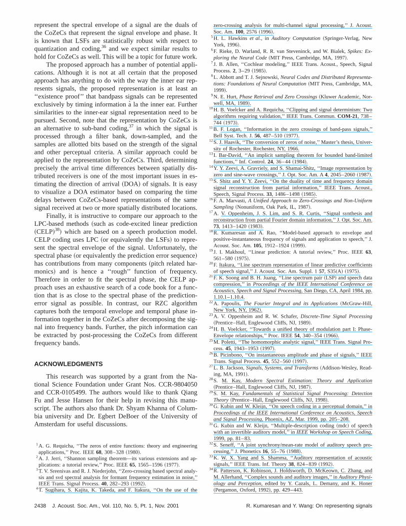
through a physiologically motivated auditory filter bank. Thspeech signal corresponds to the spoken utterance ‘‘Sheyour dark suit in greasy wash water all year’’ by a femaspeaker~timit/train/dr1/fcjf0/sa1.wav!. The original wave-form is sampled at 16 kHz. We consider only samples windices 2000 to 9150, which corresponds to the uttera‘‘She had.’’ The signal is preemphasized using a filter withtransfer function 120.98z21. Our analysis and synthesisystem is the same as in Fig. 12, but with different analyand synthesis filters. The analysis filter bank is similarthose used in many other physiologically motivated auditmodels,30–33which simulates the motion of the basilar membrane. We use the well-known gamma-tone filter bank,34 forthis purpose. The magnitude responses of 23-channel fiused in this filter bank are shown in Fig. 17~a!. It is designedby using an auditory toolbox provided by Malcolm Slaney35

As in the previous section the output of each gamma-tfilter is viewed through sliding observation windows. Wchoose a longer window (T527.5 ms) in the low-frequencyband ~channels 13–20! and a shorter window~T513.8 ms,

2435R. Kumaresan and Y. Wang: On representing signals

g

ed

brude

ouis

ZCo-

.

uelythe

undre-

approximately two times the pitch period! in the high-frequency band~channels 4 to 12!. The rest of the processinis identical to that described in the previous section.

Given the analysis filtersHk(z), k50,...,M21, the syn-thesis filters are chosen asGk(z)5Hk* (z), i.e., the synthesisfilter bank is just the analysis filter bank with time-reversimpulse response. This leads to good~but not perfect! signalreconstruction. If necessary, an equalizing filter bank canused to compensate for any imperfections in the reconsttion. Without this equalization we found that the magnitufluctuations are less than 2 dB@shown in Fig. 17~b!#.

We compared the reconstructed signal with and withRZC in Fig. 18, where the reconstruction without RZC

2436 J. Acoust. Soc. Am., Vol. 110, No. 5, Pt. 1, Nov. 2001

ec-

t

plotted in the top panel and the reconstruction with the Ralgorithm is displayed in the bottom panel. Clearly, the CZeCs represent the speech signal reasonably accurately

VII. CONCLUSIONS

From Logan’s work11 it is clear that traditional zerocrossings of a real-valued bandpass signal cannot uniqrepresent it, except in some special cases mentioned inIntroduction. Hence, in this paper, we have sought and foalternate signal-adaptive methods that can be used to

sig-c-ndat

FIG. 16. Spectrograms of the reconstructed speechnal with and without RZC: The figures show the spetrograms of the reconstructed speech signal with awithout RZC and the difference signal. Again, note ththe error contribution at lower frequencies is larger.

R. Kumaresan and Y. Wang: On representing signals

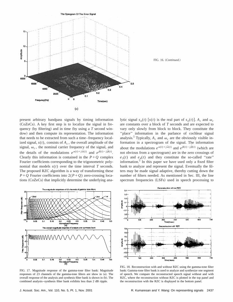
FIG. 16. ~Continued.!

io-

ioca

nd

ly

s

-

toel

on

f’’er

fil-theneto

udltermentwith

and

present arbitrary bandpass signals by timing informat~CoZeCs!. A key first step is to localize the signal in frequency~by filtering! and in time~by using aT second win-dow! and then compute its representation. The informatthat needs to be extracted from such a time–frequency loized signal,s(t), consists ofAc , the overall amplitude of thesignal,vc , the nominal carrier frequency of the signal, a

the details of the modulationsea(t)1 j a(t) and eb(t)2 j b(t).Clearly this information is contained in theP1Q complexFourier coefficients corresponding to the trigonometric ponomial that modelss(t) over the time intervalT seconds.The proposed RZC algorithm is a way of transforming theP1Q Fourier coefficients into 2(P1Q) zero-crossing loca-tions ~CoZeCs! that implicitly determine the underlying ana

FIG. 17. Magnitude response of the gamma-tone filter bank: Magnitresponses of 23 channels of the gamma-tone filters are show in~a!. Theoverall response of the analysis and synthesis filter bank is shown in~b!. Thecombined analysis–synthesis filter bank exhibits less than 2 dB ripple.

J. Acoust. Soc. Am., Vol. 110, No. 5, Pt. 1, Nov. 2001

n

nl-

-

e

lytic signal sa(t) @s(t) is the real part ofsa(t)#. Ac andvc

are constants over a block ofT seconds and are expectedvary only slowly from block to block. They constitute th‘‘place’’ information in the parlance of cochlear signaanalysis.5 Typically, Ac andvc are the obviously visible in-formation in a spectrogram of the signal. The informati

about the modulationsea(t)1 j a(t) and eb(t)2 j b(t) ~which arenot obvious from a spectrogram! are in the zero crossings oe3(t) and e4(t) and they constitute the so-called ‘‘rateinformation.5 In this paper we have used only a fixed filtbank to analyze and represent the signal. Eventually theters may be made signal adaptive, thereby cutting downnumber of filters needed. As mentioned in Sec. III, the lispectrum frequencies~LSFs! used in speech processing

eFIG. 18. Reconstruction with and without RZC using the gamma-tone fibank: Gamma-tone filter bank is used to analyze and synthesize one segof speech. We compare the reconstructed speech signal without andRZC, where the reconstruction without RZC is plotted in the top panelthe reconstruction with the RZC is displayed in the bottom panel.

2437R. Kumaresan and Y. Wang: On representing signals

lsset

ok.peet

ntr

bs

thgnbinise

msanshene

the

.apuniohmesia

re

Na05nnmof

in

a

ase

th

ust.

al

a-

o

ls,’’

er-

d

by

int.,

m

ndm.

and,’’ J.

nts

n

e-

o-

EE

n

on

inech

ro-

tic

nd

r

represent the spectral envelope of a signal are the duathe CoZeCs that represent the signal envelope and phais known that LSFs are statistically robust with respectquantization and coding,36 and we expect similar results thold for CoZeCs as well. This will be a topic for future wor

The proposed approach has a number of potential apcations. Although it is not at all certain that the proposapproach has anything to do with the way the inner ear rresents signals, the proposed representation is at leas‘‘existence proof’’ that bandpass signals can be represeexclusively by timing information a` la the inner ear. Furthesimilarities to the inner-ear signal representation need topursued. Second, note that the representation by CoZeCan alternative to sub-band coding,37 in which the signal isprocessed through a filter bank, down-sampled, andsamples are allotted bits based on the strength of the siand other perceptual criteria. A similar approach couldapplied to the representation by CoZeCs. Third, determinprecisely the arrival time differences between spatially dtributed receivers is one of the most important issues intimating the direction of arrival~DOA! of signals. It is easyto visualize a DOA estimator based on comparing the tidelays between CoZeCs-based representations of thesignal received at two or more spatially distributed locatio

Finally, it is instructive to compare our approach to tLPC-based methods~such as code-excited linear predictio~CELP!38! which are based on a speech production modCELP coding uses LPC~or equivalently the LSFs! to repre-sent the spectral envelope of the signal. Unfortunately,spectral phase~or equivalently the prediction error sequenc!has contributions from many components~pitch related har-monics! and is hence a ‘‘rough’’ function of frequencyTherefore in order to fit the spectral phase, the CELPproach uses an exhaustive search of a code book for a ftion that is as close to the spectral phase of the predicterror signal as possible. In contrast, our RZC algoritcaptures both the temporal envelope and temporal phasformation together in the CoZeCs after decomposing thenal into frequency bands. Further, the pitch information cbe extracted by post-processing the CoZeCs from diffefrequency bands.

ACKNOWLEDGMENTS

This research was supported by a grant from thetional Science Foundation under Grant Nos. CCR-9804and CCR-0105499. The authors would like to thank QiaFu and Jesse Hansen for their help in revising this mascript. The authors also thank Dr. Shyam Khanna of Colubia university and Dr. Egbert DeBoer of the UniversityAmsterdam for useful discussions.

1A. G. Requicha, ‘‘The zeros of entire functions: theory and engineerapplications,’’ Proc. IEEE68, 308–328~1980!.

2A. J. Jerri, ‘‘Shannon sampling theorem—its various extensions andplications: a tutorial review,’’ Proc. IEEE65, 1565–1596~1977!.

3T. V. Sreenivas and R. J. Niederjohn, ‘‘Zero-crossing based spectral ansis and svd spectral analysis for formant frequency estimation in noiIEEE Trans. Signal Process.40, 282–293~1992!.

4T. Sugihara, S. Kajita, K. Takeda, and F. Itakura, ‘‘On the use of

2438 J. Acoust. Soc. Am., Vol. 110, No. 5, Pt. 1, Nov. 2001

of. Ito

li-dp-an

ed

eis

eal

eg-s-

eme.

l.

e

-c-

n-

in-g-nnt

-0

gu--

g

p-

ly-,’’

e

zero-crossing analysis for multi-channel signal processing,’’ J. AcoSoc. Am.100, 2576~1996!.

5H. L. Hawkins et al., in Auditory Computation~Springer-Verlag, NewYork, 1996!.

6F. Rieke, D. Warland, R. R. van Steveninck, and W. Bialek,Spikes: Ex-ploring the Neural Code~MIT Press, Cambridge, MA, 1997!.

7J. B. Allen, ‘‘Cochlear modeling,’’ IEEE Trans. Acoust., Speech, SignProcess.2, 3–29~1985!.

8L. Abbott and T. J. Sejnowski,Neural Codes and Distributed Representtions: Foundations of Neural Computation~MIT Press, Cambridge, MA,1999!.

9N. E. Hurt,Phase Retrieval and Zero Crossings~Kluwer Academic, Nor-well, MA, 1989!.

10H. B. Voelcker and A. Requicha, ‘‘Clipping and signal determinism: Twalgorithms requiring validation,’’ IEEE Trans. Commun.COM-21, 738–744 ~1973!.

11B. F. Logan, ‘‘Information in the zero crossings of band-pass signaBell Syst. Tech. J.56, 487–510~1977!.

12S. J. Haavik, ‘‘The conversion of zeros of noise,’’ Master’s thesis, Univsity of Rochester, Rochester, NY, 1966.

13I. Bar-David, ‘‘An implicit sampling theorem for bounded band-limitefunctions,’’ Inf. Control.24, 36–44~1984!.

14Y. Y. Zeevi, A. Gravriely, and S. Shamai-Shitz, ‘‘Image representationzero and sine-wave crossings,’’ J. Opt. Soc. Am. A4, 2045–2060~1987!.

15S. Shitz and Y. Y. Zeevi, ‘‘On the duality of time and frequency domasignal reconstruction from partial information,’’ IEEE Trans. AcousSpeech, Signal Process.33, 1486–1498~1985!.

16F. A. Marvasti,A Unified Approach to Zero-Crossings and Non-UniforSampling~Nonuniform, Oak Park, IL, 1987!.

17A. V. Oppenheim, J. S. Lim, and S. R. Curtis, ‘‘Signal synthesis areconstruction from partial Fourier domain information,’’ J. Opt. Soc. A73, 1413–1420~1983!.

18R. Kumaresan and A. Rao, ‘‘Model-based approach to envelopepositive-instantaneous frequency of signals and application to speechAcoust. Soc. Am.105, 1912–1924~1999!.

19J. I. Makhoul, ‘‘Linear prediction: A tutorial review,’’ Proc. IEEE63,561–580~1975!.

20F. Itakura, ‘‘Line spectrum representation of linear predictive coefficieof speech signal,’’ J. Acoust. Soc. Am. Suppl. 157, S35~A! ~1975!.

21F. K. Soong and B. H. Juang, ‘‘Line spectrum pair~LSP! and speech datacompression,’’ inProceedings of the IEEE International Conference oAcoustics, Speech and Signal Processing, San Diego, CA, April 1984, pp.1.10.1–1.10.4.

22A. Papoulis,The Fourier Integral and its Applications~McGraw-Hill,New York, NY, 1962!.

23A. V. Oppenheim and R. W. Schafer,Discrete-Time Signal Processing~Prentice–Hall, Englewood Cliffs, NJ, 1989!.

24H. B. Voelcker, ‘‘Towards a unified theory of modulation part I: PhasEnvelope relationships,’’ Proc. IEEE54, 340–354~1966!.

25M. Poletti, ‘‘The homomorphic analytic signal,’’ IEEE Trans. Signal Prcess.45, 1943–1953~1997!.

26B. Picinbono, ‘‘On instantaneous amplitude and phase of signals,’’ IETrans. Signal Process.45, 552–560~1997!.

27L. B. Jackson,Signals, Systems, and Transforms~Addison-Wesley, Read-ing, MA, 1991!.

28S. M. Kay, Modern Spectral Estimation: Theory and Applicatio~Prentice–Hall, Englewood Cliffs, NJ, 1987!.

29S. M. Kay, Fundamentals of Statistical Signal Processing: DetectiTheory~Prentice–Hall, Englewood Cliffs, NJ, 1998!.

30G. Kubin and W. Kleijn, ‘‘On speech coding in a perceptual domain,’’Proceedings of the IEEE International Conference on Acoustics, Speand Signal Processing, Phoenix, AZ, Mar. 1999, pp. 205–208.

31G. Kubin and W. Kleijn, ‘‘Multiple-description coding~mdc! of speechwith an invertible auditory model,’’ inIEEE Workshop on Speech Coding,1999, pp. 81–83.

32S. Seneff, ‘‘A joint synchrony/mean-rate model of auditory speech pcessing,’’ J. Phonetics16, 55–76~1988!.

33K. W. X. Yang and S. Shamma, ‘‘Auditory representation of acoussignals,’’ IEEE Trans. Inf. Theory38, 824–839~1992!.

34R. Patterson, K. Robinson, J. Holdsworth, D. McKeown, C. Zhang, aM. Allerhand, ‘‘Complex sounds and auditory images,’’ inAuditory Physi-ology and Perception, edited by Y. Cazals, L. Demany, and K. Hone~Pergamon, Oxford, 1992!, pp. 429–443.

R. Kumaresan and Y. Wang: On representing signals

.,

linon

ed

-

35M. Slaney, ‘‘Auditory toolbox,’’ Tech. Rep. 45, Apple Computer, Inc1994.

36J. S. Erkelens and P. M. T. Broerson, ‘‘On the statistical properties ofspectrum pairs,’’ inProceedings of the IEEE International ConferenceAcoustics, Speech and Signal Processing, Detroit, MI, May 1995, pp.768–771.

J. Acoust. Soc. Am., Vol. 110, No. 5, Pt. 1, Nov. 2001

e

37R. V. Cox, ‘‘New directions in sub-band coding,’’ IEEE Trans. SelectAreas Commun.6, 391–409~1988!.

38M. R. Schroeder and B. Atal, ‘‘Code-excited linear prediction~celp!: Highquality speech at very low bit rates,’’ inProceedings of the IEEE International Conference on Acoustics, Speech and Signal Processing, Tampa,FL, April 1985, p. 937.

2439R. Kumaresan and Y. Wang: On representing signals