MATHEMATICA APPLICANDA

Vol. 40(1) 2012, p. 15–25

Jacek Miękisz (Warsaw)Paulina Szymańska (Warsaw)

On Spins and Genes

Abstract Many processes in natural and social sciences can be modeled by systemsof interacting objects. It is usually very difficult to obtain analytic expressions de-scribing time evolution and equilibrium behavior of such systems. Very often we relyonly on computer simulations. Fortunately, in many cases one can construct usefulapproximation schemes and derive exact results which capture some specific featuresof a given process. A frequent approach is to replace interactions between objects by amean interaction. Here we illustrate a self-consistent mean-field approximation in twoexamples: the Ising model of interacting spins and a simple model of a self-regulatinggene.

2010 Mathematics Subject Classification: 00A71; 65D17; 68U10.

Key words and phrases: Ising model, self-regulating gene, mean-field approximation.

1. Introduction. Many socio-economic and biological processes can be mod-eled by systems of interacting objects; see for example statistical mechanics andquantitative biology archives [1]. One may then try to derive their global behaviorfrom individual interactions between their basic entities such as protein moleculesin gene regulation and signaling pathway networks, animals in ecological and evolu-tionary models, and people in social processes. Such an approach is fundamental instatistical physics which deals with systems of interacting particles. One can there-fore try to apply methods of statistical physics to investigate population dynamicsand equilibrium properties of systems of interacting proteins or people.

Although interactions in such models are usually local, they propagate in spaceand as a result even faraway objects are correlated. This makes the rigorous math-ematical analysis of such systems very difficult if not impossible. Therefore, mostof such models are investigated only by means of computer simulations. But do wereally have to make such a dramatic decision either to try to prove theorems rele-vant for our models of real phenomena or just to simulate behavior of these modelson computers? Fortunately, there is a middle ground of approximations. Approxi-mations can be seen as abstractions. Following our heuristic understanding of thenature of a physical or biological process, we make an ansatz (a new model of reality)

16 On Spins and Genes

and then we try to derive in a rigorous way properties of this new model and in thisway increase our understanding of the process. Of course our new model is less fun-damental than the original one and usually we cannot estimate an error introducedby our approximation. We may lose some important features hidden in correlationsnot taken into account in our approximation. Nevertheless, in many cases we maysolve our new model analytically and derive valuable formulas.

We would like to present here a method of self-consistent mean-field approxima-tion. The core idea is as follows. The force exerted on a given object, coming fromits neighbors, is replaced by an unknown mean force - a mean field. Given the meanfield, we can easily calculate the expected value of the state of the object in theequilibrium (a stationary state of an appropriate dynamics). Now one can computethe value of the mean field and it should be consistent with the unknown value in-troduced in the beginning. One may expect (on the basis of an appropriate law oflarge numbers) that the mean-field approximation becomes exact when the numberof neighbors tends to infinity.

We illustrate the above approach in two examples: the ferromagnetic Ising modelof interacting spins located on a regular lattice and a simple model of a self-repressinggene.

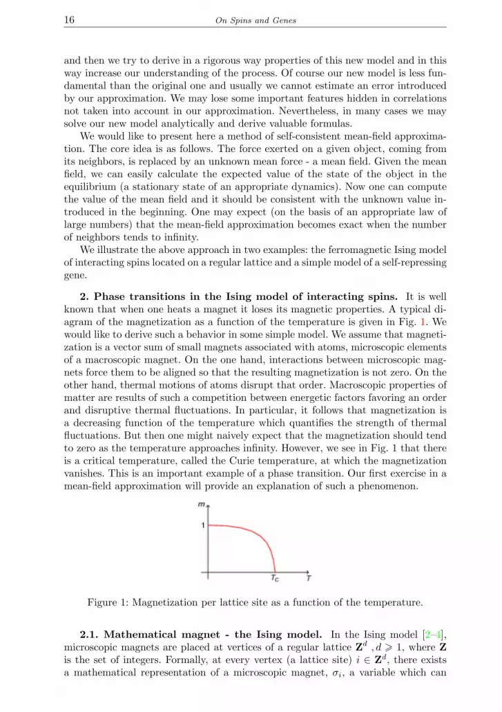
2. Phase transitions in the Ising model of interacting spins. It is wellknown that when one heats a magnet it loses its magnetic properties. A typical di-agram of the magnetization as a function of the temperature is given in Fig. 1. Wewould like to derive such a behavior in some simple model. We assume that magneti-zation is a vector sum of small magnets associated with atoms, microscopic elementsof a macroscopic magnet. On the one hand, interactions between microscopic mag-nets force them to be aligned so that the resulting magnetization is not zero. On theother hand, thermal motions of atoms disrupt that order. Macroscopic properties ofmatter are results of such a competition between energetic factors favoring an orderand disruptive thermal fluctuations. In particular, it follows that magnetization isa decreasing function of the temperature which quantifies the strength of thermalfluctuations. But then one might naively expect that the magnetization should tendto zero as the temperature approaches infinity. However, we see in Fig. 1 that thereis a critical temperature, called the Curie temperature, at which the magnetizationvanishes. This is an important example of a phase transition. Our first exercise in amean-field approximation will provide an explanation of such a phenomenon.

Figure 1: Magnetization per lattice site as a function of the temperature.

2.1. Mathematical magnet - the Ising model. In the Ising model [2–4],microscopic magnets are placed at vertices of a regular lattice Zd , d ­ 1, where Zis the set of integers. Formally, at every vertex (a lattice site) i ∈ Zd, there existsa mathematical representation of a microscopic magnet, σi, a variable which can

J. Miękisz, P. Szymańska 17

attain one of two values: +1 (a magnet directed up) and −1 (a magnet directeddown). Variables σi are called spins. The set of infinite configurations of our systemis given by Ω = +1,−1Zd , that is by the set of all functions assigning +1 or−1 to every lattice site. For a given configuration X ∈ Ω, Xi = σi(X) is called aconfiguration at the site i ∈ Zd. Let Λ ⊂ Zd be a finite subset of sites of an infinitelattice. ΩΛ = +1,−1Λ is the set of configurations on Λ. Hamiltonian (an energyfunctional) describes the energy of configurations on Λ.

HΛ : ΩΛ → R (1)

We assume that spins interact only with their nearest neighbors,

HΛ = −∑i,j∈Λ

σiσj − h∑i∈Λ

σi, (2)

where in the first sum i and j are nearest neighbors (for example j is the up, down,left, or right neighbor of i on the two-dimensional square lattice) and h is an exteriormagnetic field.

Hamiltonian in classical mechanics of interacting particles is a sum of the kineticenergy of particles and the potential energy of interactions between them. In theabove expression we do not consider the potential energy.

Our spin system is subject to thermal fluctuations and so it is a stochastic sys-tem whose time evolution can be described by an appropriate Markov chain. Thestationary state of such a Markov chain, that is a probability measure on ΩΛ isinterpreted as an equilibrium state of a physical system of interacting spins. Allmacroscopic properties, such as the energy and the magnetization of the system, arerandom variables defined on ΩΛ. We will be interested in expected values of suchrandom variables.

We introduce the following probability mass function,

ρT,hΛ (X) =e−

1T HΛ(X)

Z(T, h,Λ), (3)

where T is the temperature of the system and

Z(T, h,Λ) =∑X∈ΩΛ

e−1T HΛ(X) (4)

is a normalizing factor. Z is the so-called statistical sum and ρT,hΛ the grand-canonicalensemble. These are basic objects of statistical physics. There are many fundamen-tal explanations why the above probability mass function gives us stationary prob-abilities of our physical system. Here we will simply assume this and then drawconclusions.

Another important quantity in statistical physics is the free energy also calledthe thermodynamic potential,

F (T, h,Λ) = −T lnZ(T, h,Λ). (5)

It is worth mentioning here that one of the fundamental and still unsolved problemsin statistical physics is to derive an analytic expression for the free energy in thethree-dimensional Ising model (d = 3) in the thermodynamic limit, that is in thelimit of the infinite Λ,

18 On Spins and Genes

f(T, h) = limΛ→Z3

F (T, h,Λ)|Λ|

. (6)

It is a classical theorem that such a limit exists if Λ approaches Zd in some niceway. Calculating f(T, h) in the one-dimensional Ising model is an easy exercise, thetwo-dimensional case for h = 0 was solved by a Nobel laureate Lars Onsager [5].

Now we define the macroscopic magnetization per lattice site,

MΛ =1|Λ|∑i∈Λ

σi (7)

To avoid unnecessary technicalities, we introduce now periodic boundary conditions,that is we turn Λ into a d-dimensional torus. Let m be the expected value of therandom variable M with respect to the probability mass function ρT,hΛ , that is

m =

∑X∈ΩΛ

MΛ(X)e−1T HΛ(X)

Z(T, h,Λ). (8)

We take into account periodic boundary conditions and write the above expressionas

m =

∑X∈ΩΛ

σoe1T (∑

i,j∈Λσiσj+h

∑i∈Λ

σi)

Z(T, h,Λ), (9)

where o is any fixed site, o ∈ Λ.The presence of the sum

∑i,j σiσj in the above formula prevents us from ex-

pressing m in terms of elementary functions. Now comes the most important stepin our calculations. We introduce a mean-field ansatz and replace random variablesσj by their unknown expected value m. Every spin interacts with his 2d nearestneighbors and hence we replace

∑i,j σiσj by

∑i∈Λ 2dmσi [2, 4]. Now the exponent

both in the numerator and in the denominator factorizes and after simple algebraicmanipulations we get

m = tanh2dm+ h

T. (10)

Observe that the external magnetic field h is modified by the mean field 2dm whichcan be interpreted as an effective field coming from averaged interactions felt bya given spin. We are especially interested in the case of the zero external field,h = 0, that is in the case of a spontaneous magnetization. In such a case, to get aself-consistent m, we have to solve the following equation,

m = tanh2dmT

. (11)

It can be solved graphically. We look for intersections of the graph of the functionf(m) = tanh 2dm

T and the diagonal y = m, see Fig. 2. It is easy to see that for bigtemperatures, that is for T > 2d, there exists the unique solution m = 0 of (11).However, if T < TC = 2d, then there are three solutions: m = 0, and m = ±m0(T )for some positive m0(T ). TC is the critical Curie temperature at which a phasetransition takes place. Fig. 1 follows directly from Fig. 2 - we have achieved ourgoal.

J. Miękisz, P. Szymańska 19

Figure 2: Graphical solution of the mean-field equation (11).

One can prove that for T < TC the solution m = 0 is thermodynamically unsta-ble. The presence of two solutions m = ±m0(T ) is an effect of the symmetry of theHamiltonian (in the case of the zero external field, h = 0) with respect to the spinflip σi → −σi. It means that at any temperature below the critical one, there coexisttwo equilibrium macroscopic states. The situation is similar to the coexistence of iceand water at the zero Celsius temperature. However, such a mixed state is highlyunstable and we usually end up in one of the two so-called pure states.

3. A simple stochastic model of gene regulation. One of the fundamentalprocesses taking part in living cells is regulation of the gene expression. It enablescells to differentiate and adapt to a changing environment. Gene expression is a com-plex process involving many biochemical reactions with proteins being final products.Produced proteins may in turn enhance or repress the expression of other proteins.They may also regulate their own expression.

Here we will show how the mean-field approximation, described in the previoussection, might be used for analyzing a simple model of a self-repressing gene.

3.1. Birth and death process - the simplest model of gene expression.Birth and death processes describe the stochastic evolution of the number of certainliving objects, particles or molecules taking part in chemical reactions. It is a stan-dard assumption in such processes that the probability of any reaction to take placein a sufficiently small time interval ∆t is proportional to its length, that is it has theform r∆t + o(∆t), where r is the intensity or the rate of the reaction and o(∆t) isa quantity of a lower order than ∆t. We also assume that the probability does notexplicitly depend on time and that events in non-overlapping time intervals are in-dependent. It is a standard theorem that there exists a stochastic process satisfyingsuch conditions.

Here we are interested in proteins. In our case there are two reactions: produc-tion of a protein molecule directly from the DNA (two fundamental biochemicalprocesses, transcription and translation, are lumped together into one process) andits degradation [6], see Fig. 3. Let n be a number of protein molecules in the cell.We assume that probabilities of reactions in a small time interval ∆t are:

• production, n→ n+ 1, : k0∆t+ o(∆t)

• degradation, n→ n− 1 : γn∆t+ o(∆t)

20 On Spins and Genes

• more than one reaction, o(∆t)

Figure 3: The simplest model of gene expression, k0 is the production rate and γ isthe degradation rate.

Let f(n, t) be the probability that there are n molecules in the cell at time t. Nowwe can write the following standard system of differential equations, the so-calledMaster equation [7]:

df(n, t)dt

= k0[f(n− 1, t)− f(n, t)] + γ[(n+ 1)f(n+ 1, t)− nf(n, t)], (12)

where we assume that f(n, t) = 0 for n < 0.The Master equation describes the conservation of the probability (in the discrete

time set-up it is an example of the high-school total probability formula). We areespecially interested in the stationary point of (12), the so-called stationary statef(n), that is we set df(n,t)

dt = 0. The resulting system of recurrence equations canbe easily solved. It is well known that the stationary probability distribution isPoissonian, that is

f(n) = e−k0γ

(k0γ )n

n!. (13)

Other solvable models of gene expression can be found in [8–13]. However, in mostcases exact solutions are not possible and we have to use approximations. Someregulatory gene networks were analyzed by appropriate linearization scheme in [14].

We will now present a general generating function approach used later in thecase of a self-repressing gene.

We define the generating function F (z, t) corresponding to f(n, t), n ­ 0,

F (z, t) =+∞∑n=0

znf(n, t). (14)

Generating functions generate moments of probability distributions,

dF (z, t)dz |z=1

= 〈n〉; d2F (z, t)dz2 |z=1

= 〈n(n− 1)〉, (15)

where by 〈x〉 we denote the expected value of the random variable x with respect tothe probability distribution f(n, t). We differentiate (14) with respect to t, use (12)and get

∂

∂tF (z, t) = (z − 1)[k0F (z, t)− γ ∂F (z, t)

∂z]. (16)

J. Miękisz, P. Szymańska 21

Now we differentiate (16) once and twice with respect to z, use (15) and get

d〈n〉dt

= k0 − γ〈n〉, (17)

d〈n(n− 1)〉dt

= 2(k0〈n〉 − γ〈n(n− 1)〉).

In the stationary state we obtain

〈n〉 =k0

γ, (18)

〈n(n− 1)〉 =k0

γ〈n〉,

which gives us the following formula for the variance in the stationary state,

var(n) = 〈n2〉 − (〈n〉)2 = 〈n〉 =k0

γ. (19)

We note that the variance is equal to the expected value which is not surprisingbecause we mentioned before that the birth and death process has the Poissonstationary distribution.

3.2. Self-repressing gene – a mean-field approximation at work. Ithappens frequently that proteins regulate their own production. We will discusshere the repression - protein molecules may bind to a certain promoter region oftheir own DNA and thus decrease or completely stop the transcription. Thereforewe will consider a stochastic model, where the gene (DNA) can be in two discretestates: unbound (on) denoted by 0 or bound (off) denoted by 1. In the generic case,the transcription rates for the on- and off-states are given by k0 and k1 respectively,but we set k1 = 0 as it is often done, the protein degradation rate is denoted asbefore by γ, see Fig. 4. We consider a monomer binding and thus we assume thatthe binding rate is given by βn, the rate of switching the gene on (unbinding) isdenoted by α.

Figure 4: Self-repressing gene, the unbinding and binding rates are denoted by αand β, respectively, production rates by ki, depending on the state of the gene, andthe degradation rate by γ.

22 On Spins and Genes

We introduce two probability mass functions, fi(n), i ∈ 0, 1 - a joint probabilitythat there are n protein molecules in the system and the gene (DNA) is in the statei. Now we can write the Master equation,

d

dtf0(n, t) =k0[f0(n− 1)− f0(n)] + γ[(n+ 1)f0(n+ 1)− nf0(n)]− βnf0(n) + αf1(n),

d

dtf1(n, t) =γ[nf1(n+ 1)− (n− 1)f1(n)] + βnf0(n)− αf1(n), (20)

for n ­ 1, for n = 0 we have ddtf0(0, t) = −k0f0(0) + γf0(1) and f1(0, t) = 0.

In the above equations we assumed that a bound protein molecule cannot degrade.Similar equations were considered in [12], where the formula for the stationary dis-tribution of the number of protein molecules was derived in terms of the Kummerfunctions. Our goal here is to find an explicit expression for the variance of thenumber of protein molecules in the stationary state.

Let A0 and A1 be probabilities (frequencies) that the gene is unbound or boundrespectively and the system is in the stationary state (i.e. Ai =

∑+∞n=0 fi(n), i = 0, 1).

Expressions 〈n〉i =∑+∞n=0 nfi(n) are expected numbers of protein molecules with

respect to the probability mass functions fi(n). Obviously 〈n〉 = 〈n〉0 + 〈n〉1. Weproceed now exactly in the same way as in the previous section. We introduce twogenerating functions:

F0(z, t) =+∞∑n=0

znf0(n, t), (21)

F1(z, t) =+∞∑n=0

znf1(n, t).

and get the following system of algebraic equations for the moments in the stationarystate:

A0 +A1 = 1β〈n〉0 − αA1 = 0k0A0 − γ〈n〉0 − β〈n2〉0 + α〈n〉1 = 0γA1 − γ〈n〉1 + β〈n2〉0 − α〈n〉1 = 02k0〈n〉0 + 2γ〈n〉0 − 2γ〈n2〉0 − β〈n2(n− 1)〉0 + α〈n(n− 1)〉1 = 0−2γA1 + 4γ〈n〉1 − 2γ〈n2〉1 + β〈n2(n− 1)〉0 − α〈n(n− 1)〉1 = 0

(22)

The above system of equations is not closed (unlike in the case of unregulated geneexpression analyzed in the previous section), equations for lower-order moments in-volve higher-order moments. Several concepts and techniques were developed to closesuch hierarchical systems of equations [15–17]. To deal with interactions present inauto-regulatory genetic systems, a mean-field approximation was introduced recentlyin [18]. Here we use it to close the system of equations (22). The idea is exactly thesame as in the ferromagnetic Ising model. Namely, we replace n in the switchingterm in (20) by its unknown expected value, that is instead of βnf0(n) we writeβ 〈n〉0A0

f0(n). This leads to a closed system of equations. Instead of (22) we get

J. Miękisz, P. Szymańska 23

A0 +A1 = 1β〈n〉0 − αA1 = 0k0A0 − γ〈n〉0 − β 〈n〉0A0

〈n〉0 + α〈n〉1 = 0

γA1 − γ〈n〉1 + β 〈n〉0A0〈n〉0 − α〈n〉1 = 0

2k0〈n〉0 − 2γ〈n(n− 1)〉0 − β 〈n〉0A0〈n(n− 1)〉0 + α〈n(n− 1)〉1 = 0

−2γA1 + 2γ〈n〉1 − 2γ〈n(n− 1)〉1 + β 〈n〉0A0〈n(n− 1)〉0 − α〈n(n− 1)〉1 = 0

(23)which we solve and obtain the self-consistent value for 〈n〉0, and finally the expressionfor the variance var(n) in the stationary state. In Fig. 5 we plot var(n) as a functionof logω, where ω = α

γ is the so-called adiabaticity parameter describing how fast isthe gene switching with respect to the protein degradation.

Figure 5: Variance of the number of proteins produced in the self-repressing systemas a function of log(ω), ω = α/γ.

We see that the variance is a decreasing function of the frequency of geneswitching. We recently extended the mean-field approach to a model with two genecopies [19,20].

The validity of the mean-field approximation was checked in two extreme cases:slow gene switching (where to get analytic results we used the conditional variance)and fast gene switching (where we used the so-called adiabatic approximation). Wefound that in both cases, the stationary variance of the number of protein moleculescoincides with the mean-field approximation [20].

Acknowledgments. Paulina Szymańska was supported by the EU through theEuropean Social Fund, contract number UDA-POKL.04.01.01-00-072/09-00.

References

[1] Statistical Mechanics and Quantitative Biology on xxx.lanl.gov

[2] K. Huang, Statistical Mechanics, Wiley (1963).

[3] C. J. Thompson, Mathematical Statistical Mechanics, Princeton University Press (1972).

[4] S.-K. Ma, Statistical Mechanics, World Scientific, (1985).

[5] L. Onsager, Crystal statistics. I. A two-dimensional model with an order-disorder transition,Phys. Rev. 65: 117–149 (1944).

24 On Spins and Genes

[6] T. Kepler and T. Elston, Stochasticity in transcriptional regulation: origins, consequences,and mathematical representations, Biophys. J. 81: 3116-3136 (2001).

[7] N. G. van Kampen, Stochastic processes in physics and chemistry, 2nd ed. Amsterdam:Elsevier (1997).

[8] M. Thattai and A. van Oudenaarden, Intrinsic noise in gene regulatory networks, Proc. Natl.Acad. Sci. USA. 98: 8614–8619 (2001).

[9] P. S. Swain, M. B. Elowitz, and E. D. Siggia, Intrinsic and extrinsic contributions to stochas-ticity in gene expression, Proc. Natl. Acad. Sci. USA. 99: 12795–12800 (2002).

[10] J. Paulsson, Summing up the noise in gene networks, Nature 427: 415–418 (2004).

[11] J. Paulsson, Models of stochastic gene expression, Phys. Life Rev. 2: 157–175 (2005).

[12] J. E. Hornos, D. Schultz, G. C. Innocentini, J. Wang, A. M. Walczak, J. N. Onuchic, and P.G. Wolynes, Self-regulating gene: An exact solution, Phys. Rev. E 72: 051907 (2005).

[13] P. Paszek, Modeling stochasticity in gene regulation: characterization in the terms of theunderlying distribution function, Bull. Math. Biol. 69: 1567–1601 (2007).

[14] M. Komorowski, J. Miekisz, and A. Kierzek, Translational repression contributes greater noiseto gene expression than transcriptional repression, Biophys. J. 96: 372–384 (2009).

[15] I. Nasell, An extension of the moment closure method, Theor. Pop. Biol. 64: 233–239 (2003).

[16] B. Barzel and O. Biham, Binomial moment equations for stochastic reaction systems, Phys.Rev. Lett. 106: 150602 (2011).

[17] B. Barzel, O. Biham, and R. Kupferman, Analysis of the multiplane method for stochasticsimulations of reaction networks with fluctuations, Multiscale Model. Sim. 6: 963–982 (2011).

[18] J. Ohkubo, Approximation scheme based on effective interactions for stochastic gene regula-tion, Phys. Rev. E 83: 041915 (2010).

[19] P. Szymańska, Modeling of self-regulating gene, Master thesis, University of Warsaw (2011).

[20] J. Miekisz and P. Szymańska, Gene expression in self-regulating systems with many alleles,preprint (2012).

O spinach i genach

Streszczenie. Naszym celem jest zrozumienie i przewidywanie zachowania się ukła-dów wielu oddziałujących obiektów, takich jak cząstki i spiny w fizyce statystycznejczy geny i białka w biologii molekularnej. Jako matematycy pragniemy udowad-niać twierdzenia i wyprowadzać analityczne wzory. Bardzo szybko okazuje się, że wistotnych zastosowaniach jest to niemożliwe. Co robić? Część z nas ucieka w wyrafi-nowane symulacje komputerowe. Czy nie ma innej drogi? Czy jesteśmy ograniczenido wyboru pomiędzy Matematyką i Mathematicą? Na pomoc przychodzi metoda sa-mouzgodnionego pola średniego. Ferromagnetyczny model Isinga i samoregulującysię gen zilustrują nam tę niezwykle uniwersalną metodę otrzymywania przybliżonychrozwiązań analitycznych.

Słowa kluczowe: model Isinga, temperatura krytyczna, autoregulacja genu,przybliżenie pola średniego.

Jacek Miękisz was hiking Tatra Mountains at the age of mi-nus 6 months and then he was born in Wrocław in 1956. Heinvestigated interacting suspensions in ferrofluids and receivedMaster degree in physics from Wrocław Technical Universityin 1979. Then he moved to Blacksburg, Virginia Tech, studiedinteracting spins in Ising models of ferromagnetism and gotPhD in mathematics in 1984. He spent postdoctoral years atthe University of Texas at Austin, in Louvain-la-Neuve andLeuven, studying interacting particles in lattice-gas models ofquasicrystals. Now he works at the Institute of Applied Mathe-

matics and Mechanics of the University of Warsaw and deals with interacting agentsin evolutionary games and interacting proteins in genetic regulatory networks, some-times with time delays.

Paulina Szymańska graduated from University of Warsaw in2011, her master thesis in Mathematics under the supervision ofProf. Jacek Miękisz, entitled Modeling of self-regulating gene wonthe second prize in Competition for Best Students Work In Prob-ability and Applied Mathematics, organized by the Polish Mathe-matical Society. Currently she is a PhD student at the College ofInter-Faculty Individual Studies in Mathematics and Natural Sci-ences of the University of Warsaw, working on stochastic models ofgene expression and skiing in Tatra Mountains in her free time.

Jacek MiękiszUniversity of WarsawInstitute of Applied Mathematics, Banacha 2, 02-097 Warsaw, PolandE-mail: miekisz@mimuw.edu.plURL: www.mimuw.edu.pl/ miekisz

Paulina SzymańskaUniversity of WarsawCollege of Inter-Faculty Individual Studies in Mathematics and Natural SciencesE-mail: p.szymanska@mimuw.edu.pl

(Received: 4th of July 2012)

25