JHEP11(2007)009

Published by Institute of Physics Publishing for SISSA

Received: August 18, 2007

Accepted: October 27, 2007

Published: November 6, 2007

On the all-order ε-expansion of generalized

hypergeometric functions with integer values of

parameters

Mikhail Y. Kalmykov

II. Institut fur Theoretische Physik, Universitat Hamburg,

Luruper Chausee 149, 22761 Hamburg, Germany

E-mail: kalmykov@theor.jinr.ru

Bennie F.L. Ward

Department of Physics, Baylor University,

One Bear Place, Box 97316, Waco, TX 76798-7316, U.S.A.

E-mail: BFL Ward@baylor.edu

Scott A. Yost

Department of Physics, Princeton University,

Princeton, NJ 08544, U.S.A.

E-mail: syost@princeton.edu

Abstract: We continue our study of the construction of analytical coefficients of the

epsilon-expansion of hypergeometric functions and their connection with Feynman dia-

grams. In this paper, we apply the approach of obtaining iterated solutions to the dif-

ferential equations associated with hypergeometric functions to prove the following result:

Theorem 1. The epsilon-expansion of a generalized hypergeometric function with integer

values of parameters,

pFp−1(I1 + a1ε, . . . , Ip + apε; Ip+1 + b1ε, . . . , I2p−1 + bp−1; z) ,

is expressible in terms of generalized polylogarithms with coefficients that are ratios of

polynomials.

The method used in this proof provides an efficient algorithm for calculating of the higher-

order coefficients of Laurent expansion.

Keywords: Differential and Algebraic Geometry, NLO Computations.

c© SISSA 2007 http://jhep.sissa.it/archive/papers/jhep112007009/jhep112007009.pdf

JHEP11(2007)009

Contents

1. Introduction 1

2. All-order ε-expansion of generalized hypergeometric functions with in-

teger values of parameters 4

3. Explicit expressions for the first five coefficients of the expansion 7

4. Conclusions 9

1. Introduction

Hypergeometric functions are useful in the evaluation of Feynman diagrams. See, for ex-

ample, ref. [1] for a review of how these functions arise. In this paper, we will be concerned

with the manipulation of hypergeometric functions [2, 3], by which we understand specifi-

cally

1. the reduction of the original function to a minimal set of basis functions,

2. the construction of the all-order ε-expansion of basis functions.

The ε-expansion refers to the Laurent expansion of hypergeometric functions about rational

values of their parameters in terms of known functions or perhaps new types of functions.

In the latter case, the problem remains to identify the full set of functions which must be

invented to construct this expansion for general values of the parameters.1

Problem (1) is a purely mathematical one. It is closely related with the existence

of algebraic relations between a few hypergeometric functions with values of parameters

differing by an integer, the so-called “contiguous relations” [8]. The systematic proce-

dure for solving the relevant recursion relation is based on the Grobner basis technique.

In particular, a proper solution for generalized hypergeometric functions, the so-called

“differential reduction algorithm,” was developed by Takayama [9]. (See ref. [10] for a re-

view.) By a differential reduction algorithm, we will understand a relation of the type

F (α ± j,~b; z) = Πmk=1D(α + k;~b)F (α,~b; z), where j, k are integers, ~b is a list of additional

1All these procedures coincide with standard techniques used in the analytical calculation of Feynman

diagrams. [4, 5] It has long been expected that all Feynman diagrams can be represented by some class of

hypergeometric functions. Now we can propose specifically that any Feynman diagrams can be associated

with the Gelfand-Karpanov-Zelevinskii (GKZ or A- hypergeometric function) hypergeometric functions [6].

Let us recall that Lauricella’s, Horns’ and generalized hypergeometric functions occur as special cases of

the GKZ-systems. For an introduction, we recommended ref. [7].

– 1 –

JHEP11(2007)009

parameters and D is a differential operator of the form D = A(α;~b; z) ddz

+ B(α;~b; z).2 For

Gauss hypergeometric functions, the reduction algorithm was presented in refs. [11, 12].

For generalized hypergeometric function, is it equivalent to the statement that any function

pFp−1(~a;~b; z) can be expressed as a linear combination of functions with arguments that

differ from the original ones by an integer, pFp−1(~a + ~m;~b + ~k; z), and the function’s first

p − 1 derivatives:

Rp+1(~a,~b, z) pFp−1(~a + ~m;~b + ~k; z) = (1.1)

R1(~a,~b, z)

(d

dz

) p−1

+ · · · + Rp−1(~a,~b, z)d

dz+ Rp(~a,~b, z)

pFp−1(~a;~b; z) ,

where ~m,~k are lists of integers, the Ri are polynomials in parameters ai, bj and z.

Problem (2) arises in physics in the context of the analytical calculation of Feynman

diagrams. The complete solution of this problem is still open. We will mention here some

results in this direction derived by physicists. Let us recall that there are three different

ways to describe special functions:

(i) as an integral of the Euler or Mellin-Barnes type,

(ii) by a series whose coefficients satisfy certain recurrence relations,

(iii) as a solution of a system of differential and difference equations (holonomic approach).

For functions of a single variable, all of these representations are equivalent, but some prop-

erties of the function may be more evident in one representation than another. These three

different representations have led physicists to three different approaches to developing the

ε-expansion of hypergeometric functions.

The Euler integral representation (i) was developed intensively by Davydychev, Tarasov

and their collaborators [13] and the most impressive result was the construction of the

all-order ε-expansion of Gauss hypergeometric functions in terms of Nielsen polyloga-

rithms [14]. This type of Gauss hypergeometric function is related to one-loop propagator-

type diagrams with arbitrary masses and momenta, two-loop bubble diagrams with arbi-

trary masses, and one-loop massless vertex-type diagrams.

The series representation (ii) is a very popular and intensively studied approach. The

first results of this type were derived by David Broadhurst [15] for the so-called “single

scale” diagrams, which are associated with on-shell calculations in QED or QCD, with

further developments appearing subsequently in ref. [16].3 Particularly impressive results

involving series representations were derived recently by Moch, Uwer, and Weinzierl in the

framework of the nested sum approach. [17, 18] Algorithms based on this approach have

2An algorithm of differential reduction of generalized hypergeometric functions to a minimal set allows

the calculation of any Feynman diagram that is expressible in terms of hypergeometric functions without

any reference to integration by parts or the differential equation technique. The application of this algorithm

to the calculation of Feynman diagrams will be presented in another publication.3Some relations between the Mellin-Barnes representations and series representations of Feynman dia-

grams follow from the Smirnov-Tausk approach [21].

– 2 –

JHEP11(2007)009

been implemented in computer code. [19] The series approach leads to algebraic relations

between the analytic coefficients of the ε-expansion, but does not provide a way to obtain a

reduction of the original hypergeometric function before expansion. Another limitation of

this approach is that the parameters are restricted to integer values or special combinations

of half-integer values (so-called “zero-balance” parameter sets).4

For approach (iii), obtaining iterated solutions to the proper differential equations

associated with hypergeometric functions, the first results were obtained for Gauss hyper-

geometric functions expanded about integer values of parameters. [22] In ref. [23], that

result was extended to combinations of integer and half-integer values of parameters. An

advantage of the iterated solution approach over the series approach is that it provides

a more efficient way to calculate each order of the ε-expansion, since it relates each new

term to the previously derived terms rather than having to work with an increasingly large

collection of independent sums at each subsequent order.

The aim of the present paper is to apply approach (iii) to proving the following theo-

rem:5

Theorem 1. The all-order ε-expansion of a generalized hypergeometric function pFp−1( ~A+

~aε; ~B +~bε; z), where ~A and ~B are lists of integers, are expressible in terms of generalized

polylogarithms (see eq. (1.2)) with coefficients that are ratios of polynomials.

To be specific, this means that

P (a, b, z) pFp−1( ~A + ~aε; ~B +~bε; z) =∑

R~s(z) Li~s (z) εk ,

where ~s = (s1, . . . , sl) is a multiple index and P (a, b, z), R~s(z) are polynomials. The

generalized polylogarithms are defined by the equation

Lik1,k2,...,kn(z) =

∑

m1>m2>···mn>0

zm1

mk1

1 mk2

2 · · ·mknn

, (1.2)

For completeness, we recall that generalized polylogarithms (1.2) can be expressed as iter-

ated integrals of the form

Lik1,...,kn(z) =

∫ z

0

dt

t

dt

t · · ·

dt

t︸ ︷︷ ︸

k1−1 times

dt

1 − t · · ·

dt

t

dt

t · · ·

dt

t︸ ︷︷ ︸

kn−1 times

dt

1 − t, (1.3)

where, by definition

∫ z

0

dt

t

dt

t · · ·

dt

t︸ ︷︷ ︸

k1−1 times

dt

1 − t=

∫ z

0

dt1t1

∫ t1

0

dt2t2

· · ·

∫ tk−2

0

dtk1−1

tk1−1

∫ tk1−1

0

dtk1

1 − tk1

. (1.4)

4For some new results on ε-expansions of hypergeometric functions with nonzero-balance parameter sets

of parameters (specifically, one half-integer parameter), see ref. [20].5In fact, the result expressed in this theorem can be proved within the nested sum approach [17]. How-

ever, our idea is to extend the iterated solution approach to this more complicated system and in the

process, derive a more efficient algorithm for calculating the analytical coefficients of the ε−expansion.

– 3 –

JHEP11(2007)009

The integral (1.3) is an iterated Chen integral [27] w.r.t. the differential forms ω0 = dz/z

and ω1 = dz1−z

, so that

Lik1,...,kn(z) =

∫ z

0ωk1−1

0 ω1 · · ·ωkn−10 ω1 . (1.5)

2. All-order ε-expansion of generalized hypergeometric functions with in-

teger values of parameters

In this section, we shall prove theorem 1. We begin by noting that eq. (1.2) can be written

in a slightly different form: in terms of any basic function pFp−1(~a;~b; z) and its first p − 1

derivatives,

Rp+1(~a,~b, z) pFp−1(~a + ~m;~b + ~k; z) =

R1(~a,~b, z) θ p−1 + · · · + Rp−1(~a,~b, z) θ + Rp(~a,~b, z)

pFp−1(~a;~b; z) , (2.1)

where ~m,~k are lists of integers, the Ri are polynomials in parameters ai, bj and z, and

θ = z ddz

. The essential step in proving theorem 1 is the following lemma:

Lemma 1. The all-order ε-expansion of the function pFp−1(~aε;~1 +~bε; z), is expressible in

terms of generalized polylogarithms (eq. (1.2)).

Lemma 1 could be proved in the same manner as in case of multiple (inverse) binomial

sums. This was done in ref. [17]. However, it is fruitful to prove it using the construction

of an iterated solution of the proper differential equation related to the hypergeometric

function.6 We will follow this technique here, and in the process construct an iterative

algorithm determining the analytical coefficients of the epsilon expansion.

Let us consider the differential equation for the hypergeometric function ω(z) =

pFp−1(~aε;~1 +~bε; z):

[

z

p∏

i=1

(θ + aiε) − θ

p−1∏

i=1

(θ + biε)

]

ω(z) = 0 . (2.2)

The boundary conditions for basis functions are ω(0) = 1 and θjω(z)∣∣z=0

= 0, where

j = 1, . . . , p − 1. The proper differential equation for ω(z) is valid in each order of ε.

Defining the coefficients functions wk(z) at each order by

ω(z) =∞∑

k=0

wk(z)εk, (2.3)

6The proper solution for Gauss hypergeometric functions was constructed in refs. [22, 23].

– 4 –

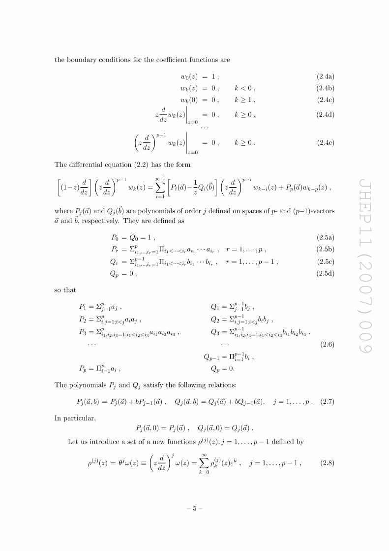
JHEP11(2007)009

the boundary conditions for the coefficient functions are

w0(z) = 1 , (2.4a)

wk(z) = 0 , k < 0 , (2.4b)

wk(0) = 0 , k ≥ 1 , (2.4c)

zd

dzwk(z)

∣∣∣∣z=0

= 0 , k ≥ 0 , (2.4d)

· · ·(

zd

dz

)p−1

wk(z)

∣∣∣∣∣z=0

= 0 , k ≥ 0 . (2.4e)

The differential equation (2.2) has the form

[

(1−z)d

dz

](

zd

dz

)p−1

wk(z) =

p−1∑

i=1

[

Pi(~a)−1

zQi(~b)

] (

zd

dz

)p−i

wk−i(z) + Pp(~a)wk−p(z) ,

where Pj(~a) and Qj(~b) are polynomials of order j defined on spaces of p- and (p−1)-vectors

~a and ~b, respectively. They are defined as

P0 = Q0 = 1 , (2.5a)

Pr = Σpi1,...,ir=1Πi1<···<irai1 · · · air , r = 1, . . . , p , (2.5b)

Qr = Σp−1i1,...,ir=1Πi1<···<irbi1 · · · bir , r = 1, . . . , p − 1 , (2.5c)

Qp = 0 , (2.5d)

so that

P1 = Σpj=1aj , Q1 = Σp−1

j=1bj ,

P2 = Σpi,j=1;i<jaiaj , Q2 = Σp−1

i,j=1;i<jbibj ,

P3 = Σpi1,i2,i3=1;i1<i2<i3

ai1ai2ai3 , Q3 = Σp−1i1,i2,i3=1;i1<i2<i3

bi1bi2bi3 .

· · · · · · (2.6)

Qp−1 = Πp−1i=1 bi ,

Pp = Πpi=1ai , Qp = 0.

The polynomials Pj and Qj satisfy the following relations:

Pj(~a, b) = Pj(~a) + bPj−1(~a) , Qj(~a, b) = Qj(~a) + bQj−1(~a), j = 1, . . . , p . (2.7)

In particular,

Pj(~a, 0) = Pj(~a) , Qj(~a, 0) = Qj(~a) .

Let us introduce a set of a new functions ρ(j)(z), j = 1, . . . , p − 1 defined by

ρ(j)(z) = θjω(z) ≡

(

zd

dz

)j

ω(z) =∞∑

k=0

ρ(j)k (z)εk , j = 1, . . . , p − 1 , (2.8)

– 5 –

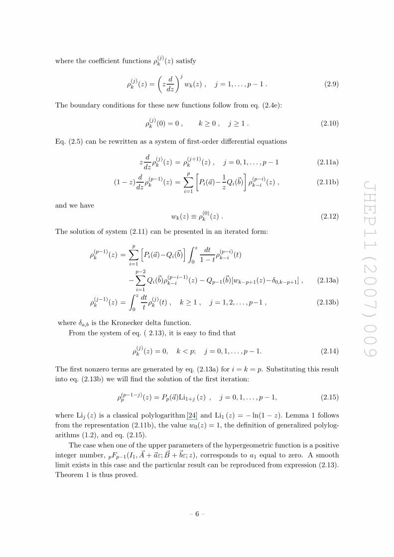
JHEP11(2007)009

where the coefficient functions ρ(j)k (z) satisfy

ρ(j)k (z) =

(

zd

dz

)j

wk(z) , j = 1, . . . , p − 1 . (2.9)

The boundary conditions for these new functions follow from eq. (2.4e):

ρ(j)k (0) = 0 , k ≥ 0 , j ≥ 1 . (2.10)

Eq. (2.5) can be rewritten as a system of first-order differential equations

zd

dzρ(j)k (z) = ρ

(j+1)k (z) , j = 0, 1, . . . , p − 1 (2.11a)

(1 − z)d

dzρ(p−1)k (z) =

p∑

i=1

[

Pi(~a)−1

zQi(~b)

]

ρ(p−i)k−i (z) , (2.11b)

and we have

wk(z) ≡ ρ(0)k (z) . (2.12)

The solution of system (2.11) can be presented in an iterated form:

ρ(p−1)k (z) =

p∑

i=1

[

Pi(~a)−Qi(~b)] ∫ z

0

dt

1 − tρ(p−i)k−i (t)

−

p−2∑

i=1

Qi(~b)ρ(p−i−1)k−i (z) − Qp−1(~b)[wk−p+1(z)−δ0,k−p+1] , (2.13a)

ρ(j−1)k (z) =

∫ z

0

dt

tρ(j)k (t) , k ≥ 1 , j = 1, 2, . . . , p−1 , (2.13b)

where δa,b is the Kronecker delta function.

From the system of eq. ( 2.13), it is easy to find that

ρ(j)k (z) = 0, k < p; j = 0, 1, . . . , p − 1. (2.14)

The first nonzero terms are generated by eq. (2.13a) for i = k = p. Substituting this result

into eq. (2.13b) we will find the solution of the first iteration:

ρ(p−1−j)p (z) = Pp(~a)Li1+j (z) , j = 0, 1, . . . , p − 1, (2.15)

where Lij (z) is a classical polylogarithm [24] and Li1 (z) = − ln(1 − z). Lemma 1 follows

from the representation (2.11b), the value w0(z) = 1, the definition of generalized polylog-

arithms (1.2), and eq. (2.15).

The case when one of the upper parameters of the hypergeometric function is a positive

integer number, pFp−1(I1, ~A + ~aε; ~B + ~bε; z), corresponds to a1 equal to zero. A smooth

limit exists in this case and the particular result can be reproduced from expression (2.13).

Theorem 1 is thus proved.

– 6 –

JHEP11(2007)009

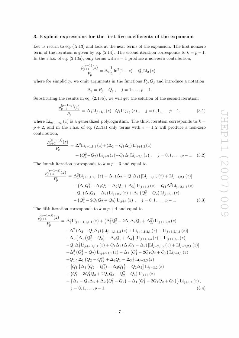
3. Explicit expressions for the first five coefficients of the expansion

Let us return to eq. ( 2.13) and look at the next terms of the expansion. The first nonzero

term of the iteration is given by eq. (2.14). The second iteration corresponds to k = p + 1.

In the r.h.s. of eq. (2.13a), only terms with i = 1 produce a non-zero contribution,

ρ(p−1)p+1 (z)

Pp

= ∆11

2ln2(1 − z) − Q1Li2 (z) ,

where for simplicity, we omit arguments in the functions Pj , Qj and introduce a notation

∆j = Pj − Qj , j = 1, . . . , p − 1.

Substituting the results in eq. (2.13b), we will get the solution of the second iteration:

ρ(p−1−j)p+1 (z)

Pp= ∆1Lij+1,1 (z)−Q1Li2+j (z) , j = 0, 1, . . . , p − 1, (3.1)

where Lia1,...,ak(z) is a generalized polylogarithm. The third iteration corresponds to k =

p + 2, and in the r.h.s. of eq. (2.13a) only terms with i = 1, 2 will produce a non-zero

contribution,

ρ(p−1−j)p+2 (z)

Pp= ∆2

1Lij+1,1,1 (z)+(∆2 − Q1∆1) Lij+1,2 (z)

+(Q2

1−Q2

)Lij+3 (z)−Q1∆1Lij+2,1 (z) , j = 0, 1, . . . , p − 1. (3.2)

The fourth iteration corresponds to k = p + 3 and equal to

ρ(p−1−j)p+3 (z)

Pp= ∆3

1Lij+1,1,1,1 (z) + ∆1 (∆2 − Q1∆1) [Lij+1,1,2 (z) + Lij+1,2,1 (z)]

+(∆1Q

21 − ∆1Q2 − ∆2Q1 + ∆3

)Lij+1,3 (z) − Q1∆

21Lij+2,1,1 (z)

+Q1 (∆1Q1 − ∆2) Lij+2,2 (z) + ∆1

(Q2

1 − Q2

)Lij+3,1 (z)

−(Q3

1 − 2Q1Q2 + Q3

)Lij+4 (z) , j = 0, 1, . . . , p − 1. (3.3)

The fifth iteration corresponds to k = p + 4 and equal to

ρ(p−1−j)p+4 (z)

Pp= ∆4

1Lij+1,1,1,1,1 (z) +(∆2

1Q21 − 2∆1∆2Q1 + ∆2

2

)Lij+1,2,2 (z)

+∆21 (∆2 − Q1∆1) [Lij+1,1,1,2 (z) + Lij+1,1,2,1 (z) + Lij+1,2,1,1 (z)]

+∆1

∆1

(Q2

1 − Q2

)− ∆2Q1 + ∆3

[Lij+1,1,3 (z) + Lij+1,3,1 (z)]

−Q1∆31Lij+2,1,1,1 (z) + Q1∆1 (∆1Q1 − ∆2) [Lij+2,1,2 (z) + Lij+2,2,1 (z)]

+∆21

(Q2

1 − Q2

)Lij+3,1,1 (z) − ∆1

(Q3

1 − 2Q1Q2 + Q3

)Lij+4,1 (z)

+Q1

∆1

(Q2 − Q2

1

)+ ∆2Q1 − ∆3

Lij+2,3 (z)

+[Q1

∆1

(Q2 − Q2

1

)+ ∆2Q1

− Q2∆2

]Lij+3,2 (z)

+(Q4

1 − 3Q21Q2 + 2Q1Q3 + Q2

2 − Q4

)Lij+5 (z)

+∆4 − Q1∆3 + ∆2

(Q2

1 − Q2

)− ∆1

(Q3

1 − 2Q1Q2 + Q3

)Lij+1,4 (z) ,

j = 0, 1, . . . , p − 1. (3.4)

– 7 –

JHEP11(2007)009

For lower values of the index p, the following relations can be used for transforming har-

monic polylogarithms [26] to the classical [24] or Nielsen [25] ones:

Lij,1, 1, . . . , 1︸ ︷︷ ︸

p times

(z) = Sj−1,p+1(z) , (3.5a)

S0,j(z) =(−1)j

j!lnj(1 − z) , (3.5b)

Li1,2 (z) = − ln(1 − z)Li2 (z) − 2S1,2(z) , (3.5c)

Li1,3 (z) = − ln(1 − z)Li3 (z) −1

2[Li2 (z)]2 , (3.5d)

Li1,4 (z) = − ln(1 − z)Li4 (z) + F2(z) , (3.5e)

Li2,2 (z) =1

2[Li2 (z)]2 − 2S2,2(z) , (3.5f)

Li3,2 (z) =1

2Li2 (z) Li3 (z) +

1

2F2(z) − 2S3,2(z) , (3.5g)

Li2,3 (z) = −3

2F2(z) −

1

2Li2 (z) Li3 (z) . (3.5h)

Li1,1,2 (z) =1

2ln2(1 − z)Li2 (z) (3.5i)

+2 ln(1 − z)S1,2(z) + 3S1,3(z) ,

Li1,2,1 (z) = − ln(1 − z)S1,2(z) − 3S1,3(z) , (3.5j)

Li2,2,1 (z) + Li2,1,2 (z) = F1(z) − Li2 (z) S1,2(z) , (3.5k)

Li1,1,3 (z) + Li1,3,1 (z) =1

2ln2(1 − z)Li3 (z) +

1

2ln(1 − z) [Li2 (z)]2 (3.5l)

− ln(1 − z)S2,2(z) − Li2 (z) S1,2(z) + F1(z),

Li1,2,2 (z) = ln(1 − z)

2S2,2(z) −1

2[Li2 (z)]2

(3.5m)

+2Li2 (z) S1,2(z) − 2F1(z) ,

Li1,1,1,2 (z) + Li1,1,2,1 (z) + Li1,2,1,1 (z) = −1

6ln3(1 − z)Li2 (z) (3.5n)

−1

2ln2(1−z)S1,2(z)−ln(1−z)S1,3(z)−2S1,4(z) ,

where we have introduced two new functions related algebraically (see eqs. (2.23) – (2.25)

in ref. [23]):

F1(z) =

∫ z

0

dx

xln2(1 − x)Li2 (x) , (3.6)

F2(z) =

∫ z

0

dx

xln(1 − x)Li3 (x) . (3.7)

For completeness, we will present the values of P and Q for p = 3, 4:

• p = 3

P1(~a) = a1 + a2 + a3 , Q1(~b) = b1 + b2 ,

P2(~a) = a1a2 + a1a3 + a2a3 , Q2(~b) = b1b2 .

P3(~a) = a1a2a3 , Q3(~b) = 0 . (3.8)

– 8 –

JHEP11(2007)009

• p = 4

P1(~a) = a1+a2+a3+a4 , Q1(~b) = b1+b2+b3 ,

P2(~a) = a1a2+a1a3+a1a4+a2a3+a2a4+a3a4 , Q2(~b) = b1b2+b1b3+b2b3 .

P3(~a) = a1a2a3+a1a2a4+a2a3a4 , Q3(~b) = b1b2b3 .

P4(~a) = a1a2a3a4 , Q4(~b) = 0 . (3.9)

The first few coefficients, up to order 4, could be cross-checked using the results of ref. [28].

We would like to point out that eqs. (3.1)–(3.4) contain an explicit logarithmic singu-

larity at z = 1. It is well-known that the generalized hypergeometric function pFp−1(~a;~b; z)

converges absolutely on the unit circle |z| = 1 if

Re

p−1∑

j=1

bj −

p∑

j=1

aj

> 0.

In this case, the coefficients of the ε-expansion also converge at each order in ε. To get

a smooth limit, it is enough to rewrite eqs. (3.1)–(3.4) in terms of functions of argument

1 − z and set z = 1.

4. Conclusions

We have shown (theorem 1) that the ε-expansions of generalized hypergeometric functions

with integer values of parameters are expressible in terms of generalized polylogarithms

(see eq. (1.2)) with coefficients that are ratios of polynomials. The proof includes (i) the

differential reduction algorithm; and (ii) iterative algorithms for calculating the analytical

coefficients of the ε-expansion of basic hypergeometric functions (see eq. (2.13)). The

first five coefficients of the ε-expansion for basis hypergeometric functions are calculated

explicitly in eqs. (2.15), (3.1), (3.2), (3.3), and (3.4). The FORM [29] representations of

these expressions and the next coefficients are available via ref. [30].

Acknowledgments

This research was supported by NATO Grant PST.CLG.980342 and DOE grant DE-FG02-

05ER41399. M. Yu. K. is supported in part by BMBF 05 HT6GUA, and is thankful to

Baylor University for support of this research, and very grateful to his wife, Laura Dolchini,

for moral support while working on the paper.

References

[1] E.E. Boos and A.I. Davydychev, A method of evaluating massive Feynman integrals, Theor.

Math. Phys. 89 (1991) 1052 [Teor. Mat. Fiz. 89 (1991) 56];

V.A. Smirnov, Evaluating Feynman integrals, Springer Tracts Mod. Phys. 211 (2004) 1;

M. Argeri and P. Mastrolia, Feynman diagrams and differential equations, Int. J. Mod. Phys.

A 22 (2007) 4375 [arXiv:0707.4037].

– 9 –

JHEP11(2007)009

[2] A. Erdelyi, Higher transcendental functions, vol.1 McGraw-Hill, New York U.S.A. (1953).

[3] L.J. Slater, Generalized hypergeometric functions, Cambridge University Press, Cambridge

U.K. (1966).

[4] F.V. Tkachov, A theorem on analytical calculability of four loop renormalization group

functions, Phys. Lett. B 100 (1981) 65;

K.G. Chetyrkin and F.V. Tkachov, Integration by parts: the algorithm to calculate

β-functions in 4 loops, Nucl. Phys. B 192 (1981) 159;

O.V. Tarasov, Connection between Feynman integrals having different values of the

space-time dimension, Phys. Rev. D 54 (1996) 6479 [hep-th/9606018].

[5] A.V. Kotikov, Differential equations method: new technique for massive Feynman diagrams

calculation, Phys. Lett. B 254 (1991) 158; Differential equations method: the calculation of

vertex type Feynman diagrams, Phys. Lett. B 259 (1991) 314; Differential equation method:

the calculation of N point Feynman diagrams, Phys. Lett. B 267 (1991) 123; New method of

massive Feynman diagrams calculation, Mod. Phys. Lett. A 6 (1991) 677.

[6] I.M. Gelfand, A.V.Zelevinskii and M.M. Kapranov, Holonomic systems of equations and

series of hypergeometric type, Dokl. Akad. Nauk 295 (1987) 14.

[7] E. Cattani, Three lectures on hypergeometric functions,

http://www.famaf.unc.edu.ar/series/pdf/pdfBMat/BMat48-2.pdf.

[8] E.D. Rainville, The contiguous function relations for pFq with applications to Bateman’s Ju,v

n

and Rice’s Hn(ζ, p, v), Bull. Amer. Math. Soc. 51 (1945) 714.

[9] N. Takayama, Grobner basis and the problem of contiguous relations, Japan J. Appl. Math. 6

(1989) 147.

[10] M. Saito, B. Sturmfels and N. Takayama, Grobner deformations of hypergeometric

differential equations, Algorithms and computation in mathematics vol. 6 Springer-Verlag,

Berlin Germany (2000).

[11] C.F. Gauss, Disquisitiones generales circa seriem infinitam 1 + αβ/γx + · · · ,, gesammelte

werke, vol. 3, Teubner, Leipzig Germany;

M. Yoshida, Fuchsian differential equations, Friedr. Vieweg & Sohn, Braunschweig Germany

(1987);

K. Iwasaki, H. Kimura,S. Shimomura and M. Yoshida, From Gauss to Painleve. A modern

theory of special functions, Friedr. Vieweg & Sohn, Braunschweig Germany (1991);

T.H. Koornwinder and V.B. Kuznetsov, Gauss hypergeometric function and quadratic

R-matrix algebras, St. Petersburg Math. J. 6 (1995) 595 [math.QA/9403218];

F. Beukers, Gauss’ hypergeometric function, technical report, Utrecht University Netherlands

(2002);

R. Vidunas, Contiguous relations of hypergeometric series, J. Comp. Appl. Math. 153 (2003)

507 [math.CA/0109222].

[12] M.Y. Kalmykov, Gauss hypergeometric function: reduction, ε-expansion for

integer/half-integer parameters and Feynman diagrams, JHEP 04 (2006) 056

[hep-th/0602028].

[13] A.I. Davydychev and J.B. Tausk, Two loop selfenergy diagrams with different masses and the

momentum expansion, Nucl. Phys. B 397 (1993) 123;

– 10 –

JHEP11(2007)009

J. Fleischer, F. Jegerlehner, O.V. Tarasov and O.L. Veretin, Two-loop QCD corrections of the

massive fermion propagator, Nucl. Phys. B 539 (1999) 671 [Erratum ibid. B 571 (2000) 511]

[hep-ph/9803493];

A.I. Davydychev and A.G. Grozin, Effect of M(C) on B quark chromomagnetic interaction

and on-shell two-loop integrals with two masses, Phys. Rev. D 59 (1999) 054023

[hep-ph/9809589].

[14] A.I. Davydychev, Explicit results for all orders of the ε-expansion of certain massive and

massless diagrams, Phys. Rev. D 61 (2000) 087701 [hep-ph/9910224];

A.I. Davydychev and M.Y. Kalmykov, Some remarks on the ε-expansion of dimensionally

regulated Feynman diagrams, Nucl. Phys. 89 (Proc. Suppl.) (2000) 283 [hep-th/0005287];

New results for the ε-expansion of certain one-, two- and three-loop Feynman diagrams, Nucl.

Phys. B 605 (2001) 266 [hep-th/0012189].

[15] N. Gray, D.J. Broadhurst, W. Grafe and K. Schilcher, Three loop relation of quark (modified)

MS and pole masses, Z. Physik C 48 (1990) 673;

D.J. Broadhurst, The master two loop diagram with masses, Z. Physik C 47 (1990) 115;

Three loop on-shell charge renormalization without integration: Λ(MS)QED to four loops, Z. Physik

C 54 (1992) 599; On the enumeration of irreducible k-fold Euler sums and their roles in knot

theory and field theory, hep-th/9604128;

D.J. Broadhurst, N. Gray and K. Schilcher, Gauge invariant on-shell Z2 in QED, QCD and

the effective field theory of a static quark, Z. Physik C 52 (1991) 111;

J.M. Borwein, D.M. Bradley and D.J. Broadhurst, Evaluations of k-fold Euler/Zagier sums:

a compendium of results for arbitrary k, hep-th/9611004;

J. Fleischer and M.Y. Kalmykov, Single mass scale diagrams: construction of a basis for the

ε-expansion, Phys. Lett. B 470 (1999) 168 [hep-ph/9910223];

M.Y. Kalmykov and O. Veretin, Single-scale diagrams and multiple binomial sums, Phys.

Lett. B 483 (2000) 315 [hep-th/0004010];

[16] F. Jegerlehner, M.Y. Kalmykov and O. Veretin, MS vs pole masses of gauge bosons. II:

two-loop electroweak fermion corrections, Nucl. Phys. B 658 (2003) 49 [hep-ph/0212319];

A.I. Davydychev and M.Y. Kalmykov, Massive Feynman diagrams and inverse binomial

sums, Nucl. Phys. B 699 (2004) 3 [hep-th/0303162];

F. Jegerlehner and M.Y. Kalmykov, The O(ααs) correction to the pole mass of the t-quark

within the standard model, Nucl. Phys. B 676 (2004) 365 [hep-ph/0308216];

M.Y. Kalmykov, Series and ε-expansion of the hypergeometric functions, Nucl. Phys. 135

(Proc. Suppl.) (2004) 280 [hep-th/0406269].

[17] S. Moch, P. Uwer and S. Weinzierl, Nested sums, expansion of transcendental functions and

multi-scale multi-loop integrals, J. Math. Phys. 43 (2002) 3363 [hep-ph/0110083].

[18] S. Weinzierl, Expansion around half-integer values, binomial sums and inverse binomial sums,

J. Math. Phys. 45 (2004) 2656 [hep-ph/0402131].

[19] S. Weinzierl, Symbolic expansion of transcendental functions, Comput. Phys. Commun. 145

(2002) 357 [math-ph/0201011];

S. Moch and P. Uwer, XSummer: transcendental functions and symbolic summation in form,

Comput. Phys. Commun. 174 (2006) 759 [math-ph/0508008];

T. Huber and D. Maitre, HypExp, a Mathematica package for expanding hypergeometric

functions around integer-valued parameters, Comput. Phys. Commun. 175 (2006) 122

[hep-ph/0507094]; HypExp2, expanding hypergeometric functions about half-integer

parameters, arXiv:0708.2443.

– 11 –

JHEP11(2007)009

[20] M.Y. Kalmykov, B.F.L. Ward and S.A. Yost, Multiple (inverse) binomial sums of arbitrary

weight and depth and the all-order ε-expansion of generalized hypergeometric functions with

one half-integer value of parameter, JHEP 10 (2007) 048 [arXiv:0707.3654].

[21] V.A. Smirnov, Analytical result for dimensionally regularized massless on-shell double box,

Phys. Lett. B 460 (1999) 397 [hep-ph/9905323];

J.B. Tausk, Non-planar massless two-loop Feynman diagrams with four on- shell legs, Phys.

Lett. B 469 (1999) 225 [hep-ph/9909506].

[22] S. Oi, Representation of the Gauss hypergeometric function by multiple polylogarithms and

relations of multiple zeta values, math.NT/0405162.

[23] M.Y. Kalmykov, B.F.L. Ward and S. Yost, All order ε-expansion of Gauss hypergeometric

functions with integer and half/integer values of parameters, JHEP 02 (2007) 040

[hep-th/0612240].

[24] L. Lewin, Polylogarithms and associated functions, North-Holland, Amsterdam Netherlands

(1981).

[25] K.S. Kolbig, J.A. Mignaco and E. Remiddi, On Nielsen’s generalized polylogarithms and their

numerical calculation, BIT 10 (1970) 38 [Erratum ibid. 10 (1970) 403];

K.S. Kolbig, Nielsen’s generalized polylogarithms, SIAM J. Math. Anal. 17 (1986) 1232.

[26] E. Remiddi and J.A.M. Vermaseren, Harmonic polylogarithms, Int. J. Mod. Phys. A 15

(2000) 725 [hep-ph/9905237].

[27] K.T. Chen, Algebras of iterated path integrals and fundamental groups, Trans. Amer. Math.

Soc. 156 (1971) 359.

[28] J. Fleischer, A.V. Kotikov and O.L. Veretin, Analytic two-loop results for selfenergy- and

vertex-type diagrams with one non-zero mass, Nucl. Phys. B 547 (1999) 343

[hep-ph/9808242].

[29] J.A.M. Vermaseren, Symbolic manipulation with FORM, Computer Algebra, Amsterdam

Netherlands (1991).

[30] M.Yu. Kalmykov, Hypergeometric functions: reduction and ε-expansion,

http://theor.jinr.ru/˜kalmykov/hypergeom/hyper.html.

– 12 –