Embed Size (px)
Citation preview

arX
iv:1
202.
5197
v2 [
mat
h.A
P] 3
1 A
ug 2
012
On the Allen-Cahn/Cahn-Hilliard system with a
geometrically linear elastic energy
Thomas Blesgen∗ and Anja Schlomerkemper†
31 August 2012
Abstract
We present an extension of the Allen-Cahn/Cahn-Hilliard system which incorpo-rates a geometrically linear ansatz for the elastic energy of the precipitates. The modelcontains both the elastic Allen-Cahn system and the elastic Cahn-Hilliard system asspecial cases and accounts for the microstructures on the microscopic scale. We provethe existence of weak solutions to the new model for a general class of energy func-tionals. We then give several examples of functionals that belong to this class. Thisincludes the energy of geometrically linear elastic materials for D < 3. Moreover weshow this for D = 3 in the setting of scalar-valued deformations, which corresponds tothe case of anti-plane shear. All this is based on explicit formulas for relaxed energyfunctionals newly derived in this article for D = 1 and D = 3. In these cases we canalso prove uniqueness of the weak solutions.
1 Introduction
In this article we study the Allen-Cahn/Cahn-Hilliard model (AC-CH model for short),which combines and extends two famous diffuse interface models: the Allen-Cahn equationand the Cahn-Hilliard equation. Both have been applied successfully to model segregation,precipitation and phase change phenomena in alloys and liquid mixtures in materials science,geology, physics, and biology, among others.The AC-CH system was first introduced in [14], and its mathematical properties have beenstudied extensively, see, e.g., [3, 27] and references therein. We study here an extension ofthis model with a particular ansatz for the elastic energy.The Allen-Cahn equation was first introduced without elasticity in [1]; and the Cahn-Hilliardequation was first introduced without elasticity in [12]. The Allen-Cahn equation is asecond order partial differential equation of Ginzburg-Landau type for an unconserved order-parameter b and thus can be used to model segregation and precipitation in solids, or othermore general situations where a reordering of the crystal lattice occurs. Conversely, the
∗Max Planck Institute for Mathematics in the Sciences, Inselstraße 22, D-04103 Leipzig, Germany, email:
[email protected]†University of Wurzburg, Institute for Mathematics, Emil-Fischer-Straße 40, D-97074 Wurzburg, Ger-
many, email: [email protected]
1

Cahn-Hilliard equation is a fourth-order partial differential equation for a conserved orderparameter a striving to model phase change phenomena where one physical quantity likethe volume of the phases is preserved. Throughout the paper we set d = a+ b as this playsa special role.The Allen-Cahn system with linear elasticity was studied before in [9], the Cahn-Hilliardsystem with linear elasticity in [21], [29] and [13]. An extension of the Cahn-Hilliard systemwith geometrically linear elasticity valid for single crystals was recently found in [7] forD ≤ 2.Except for the latter work, elastic effects due to small scale microstructures within thephases have been neglected. Here we treat the combined AC-CH model with elasticity inD ≤ 3 dimensions. We state the new extended model in (1)–(3) in Section 2. This modelprovides a basis for the generalization of further existing isothermal diffuse interface models.Our definition of the extended model does not require any special assumptions (exceptregarding the regularity) on the stored energy functional W . However, for the proof ofexistence of weak solutions, we require the Assumption (A) phrased in Section 3 below.We show that Assumption (A) is satisfied in the following cases:
(i) Materials which follow the linear theory of elasticity developed by Eshelby [19] in thecontext of elastic inclusions and inhomogeneities (see a remark after Assumption (A));
(ii) materials in D ≤ 2 which are well-described by a geometrically linear theory of elas-ticity (Theorem 5, for D = 2, cf. also [10]);
(iii) materials in D = 3 which are well-described by a geometrically linear theory of elas-ticity, where the deformations are assumed to be scalar-valued functions. This corre-sponds to the situation of anti-plane shear, see below for details and cf. Theorem 5.
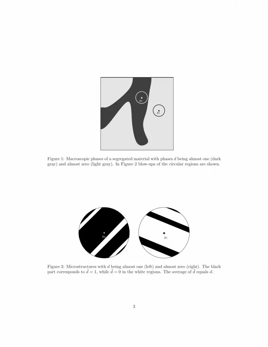
The geometrically linear theory of elasticity allows for fine microstructures within the phasesof the elastic materials taken into account. This becomes apparent in the explicit formulasfor the relaxed energy functionals, which are, together with formulas for their derivatives, thebasis of our proof of Theorem 5. In Section 4 we recall an explicit formula in D = 2 derivedby Chenchiah and Bhattacharya [15]. Moreover we prove explicit formulas for D = 1, andfor D = 3 in the setting of scalar-valued deformations. (In [15] partial results for D = 3 inthe vectorial, i.e. the non-scalar, setting are shown.)The coupling to elasticity changes significantly the morphology of the precipitates and thecoarsening patterns, see, e.g., the classification in [20]. For an intuitive picture of themicrostructures taken into account we refer the reader to Figures 1 and 2. Figure 1displays exemplary macroscopic phases of a segregated material with phases d being almostone (dark gray) and almost zero (light gray). In Figure 2 we show the correspondingmicroscopic length scale featuring microstructures; the left is a blow-up of a small regionwithin the phase with d being almost one and the right is a blow-up of a very small regionwithin the phase with d being almost zero. On this microscopic scale where we assume thatit is sufficient to treat the elastic energies of single crystals, fine microstructures in the formof laminates occur, see, e.g., [30, 22].The methods developed here apply generally to any established phase change and segre-gation model provided the temperature is conserved. (For non-isothermal settings, thevalidity of the second law of thermodynamics requires additional corrections which are not
2
y1
y2
Figure 1: Macroscopic phases of a segregated material with phases d being almost one (darkgray) and almost zero (light gray). In Figure 2 blow-ups of the circular regions are shown.
y2 y1
Figure 2: Microstructures with d being almost one (left) and almost zero (right). The blackpart corresponds to d = 1, while d = 0 in the white regions. The average of d equals d.
3

studied here.) For further discussions of our model and the analytical results we refer tothe conclusions in Section 6.
2 The AC-CH model and extensions
Throughout this paper, let Ω ⊂ RD forD ≥ 1 be a bounded domain with Lipschitz boundary
which serves as an (unstressed) reference configuration. For a stop time T > 0, let ΩT :=Ω × (0, T ) denote the space-time cylinder. To the Allen-Cahn/Cahn-Hilliard system, firstderived in [14], we add elasticity, possibly respecting the lamination microstructure, byintroducing the system
∂ta = λdiv(M(a, b)∇∂F
∂a
), (1)
∂tb = −M(a, b)∂F
∂b, (2)
0 = div (∂εW(a+ b, ε(u))) , (3)
where the function a : ΩT → R+0 is a conserved order parameter, typically a concentration,
b : ΩT → R+0 is an unconserved order-parameter, specifying the reordering of the underlying
lattice, M(a, b) denotes the positive semi-definite mobility tensor, λ > 0 is a small constantdetermining the interfacial thickness. The choice of W determines whether laminationmicrostructure occurs in the system, see (2.13).By u : Ω → R
D we describe the displacement field, such that a material point x in theundeformed body Ω is at x′ = x+ u(x) after the deformation. Then the (linearized) straintensor is defined by
ε(u) :=1
2
(∇u+∇ut
), (4)
where At denotes the transpose of a matrix A ∈ RD×D. As usual, · stands for the inner
product in RD, that is u ·v =
∑Di=1 uivi, and for A, B ∈ R
D×D we denote the inner productin R
D×D by
A :B := tr(AtB) =
D∑
i,j=1
AijBij .
Moreover, |A| :=√A :A for A ∈ R
D×D is the Frobenius norm. We denote the symmetricmatrices in R
D×D by RD×Dsym .
The functional W(a+ b, ε(u)) represents the stored elastic energy density. We will choose iteither according to the linear ansatz by Eshelby, W =Wlin, or as a single crystal compositelamination energy, W = W . The definition of W is given in the coming section 2.1.The linear theory by Eshelby [19] developed in the context of elastic inclusions and inho-mogeneities, can be summarized in the following ansatz for the elastic energy
Wlin(d, ε) :=1
2(ε− ε(d)) : C(d)(ε− ε(d)) (5)
for all ε ∈ RD×Dsym , d := a+ b, and ε(d) := d ε with a constant ε ∈ R
D×Dsym .
4

By C(d) we denote the symmetric, positive definite and concentration-dependent elasticitytensor of the system that maps symmetric tensors in R
D×D to themselves.The system (1)–(3) is completed with the definition of the free energy
F (a, b,u) :=
∫
Ω
ψ(a, b) +λ
2
(|∇a|2 + |∇b|2
)+W(a+ b, ε(u)) +Wext(ε(u)) dx, (6)
see [14], where ψ(a, b) is the free energy density assumed to be
ψ(a, b) :=ϑ
2
(g(a+ b) + g(a− b)
)+ κ1a(1 − a)− κ2b
2, (7)
g(s) := s ln s+ (1− s) ln(1− s)
for scalars κ1, κ2 > 0. The term 12 [g(a + b) + g(a − b)] in (7) defines the entropic part of
the free energy, given in the canonical Bernoulli form for perfect mixing, and ϑ > 0 is theconstant temperature.The functional Wext(ε) in (6) represents energy effects due to applied forces. In the absenceof body forces, the work necessary to transform the undeformed body Ω into a state withdisplacement u is then
−∫
∂Ω
u · σextn dS = −∫
Ω
∇u : σext dx = −∫
Ω
ε(u) : σext dx,
where we use that the applied stress σext is constant and symmetric. Consequently,
Wext(ε) = −ε : σext (8)
is the energy density of the applied outer forces. The system (1)–(3) has to be solved in ΩT
subject to the initial conditions
a(t = 0) = a0, b(t = 0) = b0 in Ω
for given functions a0, b0 : Ω → R subject to the Neumann boundary conditions for a, theno-flux boundary conditions, and the equilibrium condition for applied forces
∇a · n = ∇b · n = 0, J(a, b,u) · n = 0, σ · n = σext · n on ∂Ω, t > 0. (9)
Here, σ := ∂εW(a+ b, ε(u)) defines the stress.In (9), n is the unit outer normal to ∂Ω. For simplicity, body forces are neglected and it isassumed that the boundary tractions are dead loads given by a constant symmetric tensorσext. By J we denote the mass flux, given by
J(a, b,u) := −M(a, b)∇µ = −M(a, b)∇∂F
∂a(a, b,u),
with µ := ∂F∂a the chemical potential.
The valid parameter range of a and b is, see Theorem 1,
0 ≤ a+ b ≤ 1, 0 ≤ a− b ≤ 1. (10)
5

The inequalities are strict unless (a, b) = (0, 0) or (a, b) = (1, 0).For a0 = b0 ≡ 0 in Ω, we obtain the pathological solution a = b ≡ 0 in ΩT . For a0 ≡ 1,b0 ≡ 0 in Ω we obtain a Cahn-Hilliard equation in b and a pathological equation for a.The system (1)–(3) includes as special case the elastic Cahn-Hilliard system (setting b ≡ 0,[21])
∂ta = λdiv(M(a)∇∂F
∂a
),
0 = div (∂εW(a, ε(u)))
with
F (a,u) :=
∫
Ω
ψ(a) +λ
2|∇a|2 +W(a, ε(u)) +Wext(ε(u)) dx,
ψ(a) :=ϑ
2a lna+ (1− a) ln(1− a) + κ1a(1− a)
and the boundary and initial conditions correspondingly to above. Moreover the system(1)–(3) includes as special case the elastic Allen-Cahn equations (setting a ≡ 1
2 , [9]) whichfor rescaled b with 0 < b < 1 read
∂tb = −M(b)∂F
∂b,
0 = div (∂εW(b, ε(u))) ,
with
F (b,u) :=
∫
Ω
ψ(b) +λ
2|∇b|2 +W(b, ε(u)) +Wext(ε(u)) dx,
ψ(b) :=ϑ
2
(g(b) + g(1− b)
)+κ14
− κ2b2
and g as well as the boundary and initial conditions are as above.
6

The system (1)–(3) is exemplary for an isothermal model that exhibits simultaneous orderingand phase transitions. Equation (1) is a diffusion law for a governed by the flux J and statesthe conservation of mass in Ω. Equation (2) is a simple gradient flow in the descent direction−∂F
∂b . Equation (3) is a consequence of Newton’s second law under the additional assumptionthat the acceleration ∂ttu originally appearing on the left hand side can be neglected (thiscan be proved formally by a scaling argument and formally matched asymptotics). Thevector equation (3) serves to determine the unknown displacement u.
Remark 1. The equations (1)–(3) can be generalized to vector-valued mappings a, b. Thisallows to study situations with more than two phases present. To fix ideas and for the sakeof a clear presentation, we restrict ourselves throughout this paper to scalars a and b.
Remark 2. The equations (1)–(3) with boundary conditions (9) and (6) and (7) complywith the second law of thermodynamics, which in case of isothermal conditions reads for aclosed system
∂tF (a(t), b(t),u(t)) ≤ 0.
This inequality can be verified by direct inspection similar to the calculations in [7].
In the proof of Theorem 2 we apply the following explicit formulation of (1)–(3) with constantmobility M ≡ 1
∂ta = λ[ϑ
2
(g′(a+b) + g′(a−b)
)+ κ1(1−2a) +
∂W∂d
(a+b, ε(u))−a], (2.1’)
∂tb = λb+ ϑ
2[g′(a− b)− g′(a+ b)] + 2κ2b−
∂W∂d
(a+ b, ε(u)), (2.2’)
0 = div (∂εW(a+ b, ε(u))) . (2.3’)
The subsequent section is devoted to the geometrically linear elastic energy for single crys-tals. This is a prerequisite to the discussion of existence and uniqueness results for theextensions of the Allen-Cahn/Cahn-Hilliard (AC-CH) model studied in Section 3.
2.1 The geometrically linear theory of elasticity in single crystals
Our main objective in this subsection is to study a geometrically linear theory of elasticityin the context of isothermal phase transitions. For systematic reasons, we first recall thelinear ansatz dating back to Eshelby, [19]. As a byproduct of the existence theory proved inSection 3 we obtain a new existence result for the AC-CH equations with linear elasticity.Subsequently, we introduce the geometrically linear elasticity theory that takes the laminatesof the material into account.
In the following we assume that two phases are present in the considered material whichmay form microstructures as displayed, e.g., in Figures 3 and 4. We refer to the energy Wi,i = 1, 2 of each of the phases as microscopic energy, cf. (2.12), and to the energy W (d, ε(u))in (2.13), which reflects the effective behavior of the system with microstructures, as themacroscopic energy.To determine the energy W (d, ε(u)) in the geometrically linear theory we need to solve alocal minimization problem, Eqn. (2.13) below, which we shall outline now.
7

We assume that the volumes occupied by each of the two phases in Ω are measurable sets.In particular, if d1 ≡ d, d2 ≡ 1 − d characterize the two phases on the microscale, we havedi ∈ BV (Ω; 0, 1) and d1+ d2 = 1 a.e. in Ω. The symbol BV denotes the space of functionsof bounded variation, see, e.g., [2, 31]. By
〈 ˜〉 :=∫
Ω
− ˜(x) dx :=1
|Ω|
∫
Ω
˜(x) dx (2.11)
we denote the average of a function ˜ in Ω, where |E| is the D-dimensional Lebesgue measureof a set E.Let εTi ∈ R
D×Dsym , i = 1, 2, be the stress-free strain (or eigenstrain) of the i-th phase relative
to the chosen reference configuration and αi be its positive definite elasticity tensor. Thenthe elastic energy density of phase i subject to a strain ε is given by
Wi(ε) :=1
2αi
(ε− εTi
):(ε− εTi
)+ wi (2.12)
for wi ≥ 0. In (2.12) we assumed for simplicity that αi, εTi and wi are constants, independent
of x ∈ Ω and the order parameter d.Under the assumption that the elastic energy adapts infinitely fast and that the surfaceenergy between laminates of the microstructure can be neglected, the effective elastic energyis, [15],
W (d, ε)(y) := inf〈d〉=d(y)
d∈0,1
infu|∂Ω=ε(y)x
∫
Ω
−W (d, ε(u)) dx, d ∈ [0, 1], (2.13)
where we usedW (d, ε) := dW1(ε) + (1 − d)W2(ε), d ∈ 0, 1. (2.14)
The definition (2.13) requires further clarification. Firstly, ε = ε(u) := 12 (∇u +∇ut), and
instead of integrating over Ω, one may integrate over Br(y), the open ball of radius r aroundy ∈ Ω, where the mean 〈·〉 is now taken over Br(y). By homotopy arguments or by results
in [18], any r > 0 yields the same value of W (d, ε)(y), as long as Br(y) ⊂ Ω. Takingthe union of such balls then leads to (2.13). Secondly, the infimum over d is the result ofhomogenization subject to the constraint that the volume fraction of the selected phase ispreset by d(y), see [17, Chapter 10]. This infimum is taken over functions d ∈ BV (Ω; 0, 1)as explained above ensuring W ≥ 0. This is why (2.13) is only meaningful for d ∈ [0, 1].The second infimum is taken over functions u ∈ H1(Ω; RD) where the condition u|∂Ω =ε(y)x has to be read as u(x) = ε(y)x for a.e. x ∈ ∂Ω. This originates from the requirement
that the functional W thus defined must be quasi-convex, see [18], and is the result ofrelaxation theory, [18], [23], as follows. If for prescribed d = a + b the microscopic elasticenergy density is denoted by Wd(ε), then
Wd(ε) := infu|∂Ω=εx
∫
Ω
−Wd(ε(u)) dx (2.15)
is the elastic energy density of the material with macroscopic strain ε after microstructurehas formed. For D = 2, explicit analytic formulas for W are known, see [15] as well as
formulas of the partial derivatives of W . These will be recalled in Section 4.
8

3 Existence and uniqueness results for the AC-CH sys-
tem
The existence of solutions to the Allen-Cahn/Cahn-Hilliard equation without elasticity wasstudied in [11] with the help of a semigroup calculus. Existence and uniqueness of weaksolutions to the Cahn-Hilliard equation with linear elasticity is proved in [21], with geomet-rically linear elasticity in [7]. Existence and uniqueness of weak solutions to the Allen-Cahnequation with linear elasticity is shown in [9].Subsequently we provide existence and uniqueness results for (1)–(3), where W is an elasticenergy density satisfying the following assumption (A).
(A) The elastic energy density W ∈ C1(R× RD×Dsym ; R) satisfies the conditions
(A1) ∂εW(d, ·) is strongly monotone uniformly in d, i.e., there exists a constantc1 > 0 such that for all ε1, ε2 ∈ R
D×Dsym and all d ∈ R
(∂εW(d, ε2)− ∂εW(d, ε1)) : (ε2 − ε1) ≥ c1|ε2 − ε1|2.
(A2) There exists a constant C1 > 0 such that for all d ∈ R and all ε ∈ RD×Dsym
|W(d, ε)| ≤ C1(|d|2 + |ε|2 + 1),
|∂dW(d, ε)| ≤ C1(|d|2 + |ε|2 + 1),
|∂εW(d, ε)| ≤ C1(|d|+ |ε|+ 1).
All constants in this article, unless explicitly stated otherwise, may depend on the materialparameters α1, α2, ε
T1 and εT2 , but are independent of d and ε. Condition (A1) states that
W is convex in ε. The problem becomes non-convex through the dependence on d. Oneprominent example satisfying assumption (A) is the elastic energy Wlin in (5). In Section 5
we prove that also the relaxed energy functional W defined in (2.13) satisfies the assumption(A).We require the condition
W(a0 + b0, ε(u(x, 0))) <∞, (3.16)
where u(·, 0) is the solution of (3) for a = a0, b = b0.
Theorem 1 (Existence of weak solutions). Let the mobility tensor M be positive definiteand continuous for all a, b satisfying (10), W fulfill (A), ψ be given by (7) and the initialdata (a0, b0) satisfy (10) and (3.16). Then there exists a weak solution (a, b,u) to (1)–(3)that satisfies(i) a, b ∈ C0, 1
4
([0, T ]; L2(Ω)
),
(ii) ∂ta ∈ L2(0, T ;H1(Ω)∗), ∂tb ∈ L2(ΩT ),(iii) u ∈ L∞
(0, T ; H1(Ω; RD)
),
(iv) The feasible parameter range of (a, b) is given by (10).
Proof: The statements of the theorem can be proved with the methods developed in [9]for an Allen-Cahn system with linear elasticity and in [21] for a Cahn-Hilliard system withlinear elasticity. We sketch the main steps.
9
First we introduce the operator M associated to w 7→ −Mw as a mapping from H1(Ω)to its dual by
M(w)η :=
∫
Ω
M∇w · ∇η dx. (3.17)
From the Poincare inequality and the Lax-Milgram theorem (which can be applied since Mis assumed to be positive definite) we know that M is invertible and we denote its inverseby G, the Green’s function. We have
(M∇Gf,∇η)L2 = 〈η, f〉 for all η ∈ H1(Ω), f ∈ (H1(Ω))′.
For f1, f2 ∈ (H1(Ω))′, we define the inner product
(f1, f2)M := (M∇Gf1,∇Gf2)L2
with the corresponding norm
‖f‖M :=√(f, f)M for f ∈ (H1(Ω))′.
For a small discrete step size h > 0, chosen such that T h−1 ∈ N, for time steps m ∈ N with0 < m < T h−1, and given values am−1, bm−1 ∈ R, we introduce the discrete free energyfunctional
Fm,h(a, b,u) := F (a, b,u) +1
2h‖a− am−1‖2M +
1
2h‖b− bm−1‖2L2 , (3.18)
where (in case ofm = 1) it holds a0 = a0, b0 = b0, the initial values of a and b. By the direct
method in the calculus of variations and Assumption (A), it is possible to show that for hsufficiently small, Fm,h possesses a minimizer (am, bm,um) ∈ H1(Ω)×H1(Ω)×H1(Ω; RD).This minimizer solves the fully implicit time discretization of (1)–(3). Next the discretesolution is extended affine linearly to (a, b,u) by setting for t = (τm+(1− τ)(m−1))h withsuitable τ ∈ [0, 1]
(a, b,u)(t) := τ(am, bm,um) + (1− τ)(am−1, bm−1,um−1).
The validity of the second law of thermodynamics (cf. Remark 2) together with (3.16) impliesthat F is non-increasing in time. In combination with a higher integrability condition onu, [21], this allows to derive uniform estimates for (a, b,u). Compactness arguments thenallow to pass to the limit hց 0 and the limit solves (1)–(3).
In general, the uniqueness of solutions to (1)–(3) is open. However, we prove it in a specialcase for the linear elastic energy density W =Wlin.
Theorem 2 (Uniqueness of solutions for linear elasticity). Let W=Wlin be given by (5), thematerial be homogeneous, i.e. the elasticity tensor C be independent of d, and let M ≡ 1.Then the solution (a, b,u) of Theorem 1 is unique in the spaces stated there.
Proof: The proof is very similar to the proof of uniqueness for the Cahn-Hilliard system[21] but we repeat it here because we later need to modify it.
10

Fix t0 ∈ (0, T ). Let (ak, bk,uk), k = 1, 2 be two pairs of solutions to (2.1’)–(2.3’) and (5).The differences a := a1 − a2, b := b1 − b2, u := u1 −u2 with corresponding difference of thechemical potentials µ := µ1 − µ2 := ∂F
∂a (a1, b1)− ∂F
∂a (a2, b2) solve the weak equations
∫
ΩT
[−a∂tξ + λ∇µ · ∇ξ] dxdt = 0, (3.19)
∫
ΩT
[∂tbη + λ∇b · ∇η − ε : C (ε(u)− (a+ b)ε) η] dxdt
=
∫
ΩT
[ϑ
2
(g′(a2+b2)− g′(a1+b1) + g′(a1−b1)− g′(a2−b2)
)η + 2κ2bη
]dxdt, (3.20)
∫
Ωt0
C (ε(u)− ε(a+ b)) : ε(u) dxdt = 0 (3.21)
for every ξ, η ∈ L2(0, T ; H10 (Ω)) ∩ L∞(ΩT ) with ∂tξ, ∂tη ∈ L2(ΩT ), ξ(T ) = 0, where in
order to get (3.21) we plugged in (u2−u1)X(0,t0) as a test function and integrated by parts.As a test function in (3.19) we pick
ξ(x, t) :=
∫ t0t µ(x, s) ds, if t ≤ t0,0, if t > t0.
This shows ∫
Ωt0
aµ+ λ∇(Ga) · ∇(∂tGa) dxdt = 0. (3.22)
The difference of the chemical potentials fulfils, with the help of (6),
∫
ΩT
µζ dxdt =
∫
ΩT
[ϑ2
(g′(a1 + b1)− g′(a2 + b2) + g′(a2 − b2)− g′(a1 − b1)
)ζ
− 2κ1aζ + λ∇a · ∇ζ − ε : C(ε(u)− (a+ b)ε)ζ]dxdt.
We pick ζ := (a1 − a2)X(0,t0). With (3.22) we obtain
λ
2‖a(t0)‖2M +
∫
Ωt0
λ|∇a|2 − aε : C(ε(u) − ε(a+ b)) dxdt ≤
∫
Ωt0
2κ1a2 +
ϑ
2
[∣∣g′(a1+b1)− g′(a2+b2)∣∣+
∣∣g′(a1−b1)− g′(a2−b2)∣∣]|a| dxdt. (3.23)
In (3.20) we choose η := (b1 − b2)X(0,t0) as a test function and add the resulting equation
11

to (3.23) and use (3.21). We end up with
λ
2‖a(t0)‖2M +
1
2‖b(t0)‖L2 +
∫
Ωt0
[λ(|∇a|2 + |∇b|2
)+W(a+ b, ε(u))
]dxdt
≤∫
Ωt0
2(κ1|a|2 + κ2|b|2) dxdt
+
∫
Ωt0
ϑ
2
[∣∣g′(a1+b1)− g′(a2+b2)∣∣ +
∣∣g′(a1−b1)− g′(a2−b2)∣∣](|a|+|b|) dxdt.
From Theorem 1 we know that the terms g′(ai ± bi), i = 1, 2 are finite, and g′ is Lipschitzcontinuous. Applying first Young’s inequality, then Gronwall’s inequality, as t0 ∈ (0, T ) wasarbitrary, we find a = b = 0 in ΩT . This finally yields
∫
ΩT
ε(u) : Cε(u) dxdt = 0.
With Korn’s inequality this proves u ≡ 0 in ΩT .
4 Explicit formulas for W
In many situations like the numerical implementation of the extended models, the abovedefinition (2.13) of W is not practical since it is indirect and based on a local minimization.For these applications and for direct later use, we collect here some explicit formulas of therelaxed energy W for D ≤ 2 and for the scalar case in D = 3.
4.1 The case D = 2
As shown in [15], it holds
W (d, ε) = d1W1(ε∗1) + d2W2(ε
∗2) + β∗d1d2 det(ε
∗2 − ε∗1), (4.24)
where β∗, ε∗1 and ε∗2 are defined below. First we need to fix further notations following [15].Let γ∗ > 0 be given by
γ∗ := minγ1, γ2, (4.25)
where γi is the reciprocal of the largest eigenvalue of α−1/2i Tα
−1/2i , αi is the elastic modulus
of laminate i, and the operator T : R2×2sym → R
2×2sym is given by
Tε = ε− tr(ε)Id.
In [7] a recipe is given for the practical computation of γ∗. Here, we only remark that if thespace groups of the two existing laminates are cubic, it holds
γ∗ = minC1,11 − C1,12, C2,11 − C2,12, 2C1,44, 2C2,44.
12

The first subscript of C denotes here the phase, the other two indices are the coefficients ofthe reduced elasticity tensor in Voigt notation, [28].As shown in [15], the scalar β∗ ∈ [0, γ∗] determines the amount of translation of the laminatesdefined by
β∗ = β∗(d, ε) :=
0 if ϕ ≡ 0 (Regime 0),0 if ϕ(0, d, ε) > 0 (Regime I),βII if ϕ(0, d, ε) ≤ 0 and ϕ(γ∗, d, ε) ≥ 0 (Regime II),γ∗ if ϕ(γ∗, d, ε) < 0 (Regime III).
(4.26)
In this definition, βII = βII(d, ε) is the unique solution of ϕ(·, d, ε) = 0 with ϕ defined by
ϕ(β, d, ε) := −det(ε∗(β, d, ε)) = −det[α(β, d)−1e(ε)
], (4.27)
ε∗ = ε∗(β, d, ε) := ε∗2(β, d, ε)− ε∗1(β, d, ε),
and the yet undefined functions are specified below.
The four regimes have the following crystallographic interpretation, which follows from theconstruction of the optimal microstructure in the calculation of W .Regime 0: The material is homogeneous and the energy does not depend on the microstruc-ture. This occurs when α2(ε
T2 − ε)− α1(ε
T1 − ε) = 0.
Regime I: There exist two optimal rank-I laminates.This is characterized by
det[(d2α1 + d1α2)
−1(α2(ε
T2 − ε)− α1(ε
T1 − ε)
)]< 0.
Regime II: The unique optimal microstructure is a rank-I laminate.This regime occurs when the function
[0, γ∗] ∋ β 7→ det[(d2α1 + d1α2 − βT )−1 (α2(ε
T2 − ε)− α1(ε
T1 − ε)
)]
has a unique root (which we denote by βII).Regime III: There exist two optimal rank-II laminates. This regime is present if theoperator (d2α1 + d1α2 − γ∗T ) is invertible and
det[(d2α1 + d1α2 − γ∗T )−1 (α2(ε
T2 − ε)− α1(ε
T1 − ε)
)]> 0.
For illustration, we visualize prototypes of rank-I and rank-II laminates in Figures 3 and 4.
To complete the definition (4.27), set
α(β∗, d) := d2α1 + d1α2 − β∗T,
e(ε) := α2(εT2 − ε)− α1(ε
T1 − ε),
ε∗i ≡ ε∗i (β∗, d, ε) := α−1(β∗, d)ei(β
∗, d, ε), (4.28)
e1(β∗, d, ε) := (α2 − β∗T )ε− d2(α2ε
T2 − α1ε
T1 ),
e2(β∗, d, ε) := (α1 − β∗T )ε+ d1(α2ε
T2 − α1ε
T1 ).
13

Figure 3: A two-phase rank-I laminate in two space dimensions with corresponding normalvector. The strains are constant in the shaded and in the unshaded regions. The volumefraction of both phases, 0.5 in the picture, is prescribed by the macroscopic parameter d.
︸ ︷︷ ︸
h1
︸ ︷︷ ︸
h2
Figure 4: A two-phase rank-II laminate in two space dimensions. The widths h1 and h2 ofthe slabs should be much larger than the thickness of the layers between the slab.
Hence ε∗2 − ε∗1 = [α(β∗, d)]−1e(ε).
Explicit computations of ∂dW and ∂εW are lengthy. We recall the following results for thepartial derivatives of W in D = 2 which are proved in [7]. Set
σ∗i := αi(ε
∗i − εTi ),
σ∗ := d1σ∗1 + d2σ
∗2 .
Lemma 1. Let D = 2 and let αi and T commute. Then
∂W
∂ε(d, ε) = d1α1
(ε∗1 − εT1
)+ d2α2
(ε∗2 − εT2
)
+
γ∗d1d2α
−1(γ∗, d)(α1 − α2)T (ε∗2 − ε∗1) in Regime III
0 else.(4.29)
Alternatively, in Regime III,
∂W
∂ε(d, ε) = d1(α2 − γ∗T )α−1(γ∗, d)α1
(ε∗1(γ
∗, d, ε)− εT1)
+ d2(α1 − γ∗T )α−1(γ∗, d)α2
(ε∗2(γ
∗, d, ε)− εT2). (4.30)
14

Moreover it holds
∂W
∂d(d, ε) = σ∗ :ε∗ +W1(ε
∗1)−W2(ε
∗2) +
0 in Regimes 0 and I,
β∗d1d2∂β∗
∂d ‖ε∗‖2 in Regime II,
(d1 − d2)γ∗ϕ(ε∗) in Regime III.
(4.31)
∂β∗
∂d=
(T (d2α1+d1α2−βT )−1(α2−α1)ε∗):ε∗
((d2α1+d1α2−βT )−1(Tε∗)):Tε∗ in Regime II,
0 otherwise.(4.32)
∂β∗
∂ε=
1
((d2α1+d1α2−βT )−1(Tε∗)):Tε∗ (α1 − α2)α−1Tε∗ in Regime II,
0 otherwise.(4.33)
4.2 The scalar setting for D = 3
The scalar setting in three dimensions is characterized by the ansatz
u(x1, x2, x3) :=
x1x2
η(x1, x2)
(4.34)
for the deformation, where η is a scalar function (hence the name ’scalar’ theory, see [5],[6]). Physically, (4.34) corresponds to anti-plane shear in the x3-plane. Since
ε(u) =
1 0 ∂x1η
0 1 ∂x2η
∂x1η ∂x2
η 0
,
∇η determines the strain. This justifies to work with vectors f = ∇η ∈ R2, not with
matrices ε(u). We replace (2.13) by
W (d, f) := inf〈d〉=d
d∈0,1
infη|∂Ω′=f ·x
∫
Ω′
− d1W1(∇η) + d2W2(∇η) dx, d ∈ [0, 1], (4.35)
where the domain of integration Ω′ is now two-dimensional. Therefore, d ∈ BV (Ω′; 0, 1),and it is well-understood from the context that
〈d〉 := 1
|Ω′|
∫
Ω′
d(x) dx
denotes the two-dimensional average. In addition, in (4.35) we adapted the common notationfor the scalar case and wrote f instead of ε for the strain. Finally, we set
Wi(f) :=1
2αi(f − fT
i ) · (f − fTi ) + wi
15

with fTi the transformation strains in the scalar setting and αi positive definite matrices.
In [15], partial results for W in the non-scalar, i.e. vectorial setting are available for D = 3.
Yet, in general, the computation of ∂dW , ∂εW for D = 3 as required for assumption (A)remains currently open due to its complexity. This is the reason why we restrict ourselves toa special three-dimensional case. Our main result in this subsection is the following theoremthat provides us with an explicit formula for W in the scalar case.
Theorem 3 (Representation formula for W andD = 3 in the scalar setting). The functional
W , given by (4.35), satisfies the explicit representation formula
W (d, f) = d1W1(∇η∗1) + d2W2(∇η∗2) (4.36)
with
∇η∗1(d, f) := (d2α1 + d1α2)−1
[α2f − d2(α2f
T2 − α1f
T1 )
], (4.37)
∇η∗2(d, f) := (d2α1 + d1α2)−1
[α1f + d1(α2f
T2 − α1f
T1 )
]. (4.38)
Theorem 3 states in particular that the scalar elastic theory in 3D is directly related to thenon-scalar geometrically linear elasticity theory in 2D which was discussed in Subsection 4.1.
Proof: We apply the translation method, see for instance [16], [26] for an overview. Ingeneral, the function ϕ which describes the translation is only quasi-convex. Here, as abenefit of the scalar theory, we can pick ϕ as a convex function, cf. (4.42).Starting from the inequality
ϕ(f) ≤ infη|∂Ω′=f ·x
∫
Ω′
− ϕ(∇η) dx,
which is satisfied by any quasi-convex function ϕ, we obtain, similar to the reasoning in [15]for the non-scalar case in D = 2 dimensions,
W (d, f) ≥ maxβ≥0
Wi−βϕ convex
mind∈BV (Ω′;0,1)
〈d〉=d
infη|∂Ω′=f ·x
[∫
Ω′
− d1(W1 − βϕ)(∇η) + d2(W2 − βϕ)(∇η) dx
+ βϕ(f)
]. (4.39)
Consider
∇η1(d, η) :=∫Ω′− d1∇η dx∫Ω′− d1 dx
, ∇η2(d, η) :=∫Ω′− d2∇η dx∫Ω′− d2 dx
. (4.40)
Thend1∇η1(d, η) + d2∇η2(d, η) = f. (4.41)
Next we apply Jensen’s inequality which is possible since Wi − βϕ is convex for i = 1, 2.Furthermore we possibly enlarge the set of admissible functions in the minimization over η
16

in (4.39) by considering the set of admissible functions ∇η1,∇η2 ∈ R2 with the constraint
(4.41). Then (4.39) becomes
W (d, f) ≥ maxβ≥0
Wi−βϕ convex
min∇η1,∇η2∈R
2
d1∇η1+d2∇η2=f
d1W1(∇η1) + d2W2(∇η2) + βϕ(f)
.
If D = 2, ϕ is chosen to be − det(ε(u)). Here we set analogously
ϕ(∇η) :=(∂xη
)2+(∂yη
)2 ≥ 0. (4.42)
Since ϕ is quadratic, there exists a unique linear operator T : R2 → R2 such that ϕ(f) =
12Tf :f , here simply Tf = 2f . It holds
2∑
i=1
di(Wi − βϕ)(∇ηi) + βϕ(f)
=
2∑
i=1
diWi(∇ηi) + β[ϕ(d1∇η1 + d2∇η2)− d1ϕ(∇η1)− d2ϕ(∇η2)︸ ︷︷ ︸
=:R
].
By a direct computation the remainder term R can be rewritten,
2R = T (d1∇η1 + d2∇η2) : (d1∇η1 + d2∇η2)− d1T∇η1 :∇η1 − d2T∇η2 :∇η2= d1d2
[− T∇η1 :∇η1 − T∇η2 :∇η2 + T∇η1 :∇η2 + T∇η2 :∇η1
]
= −d1d2T (∇η2 −∇η1) : (∇η2 −∇η1)= −2d1d2ϕ(∇η2 −∇η1).
So we have found
W (d, f) ≥ maxβ≥0
Wi−βϕ convex
min∇η1,∇η2∈R
2
d1∇η1+d2∇η2=f
d1W1(∇η1) + d2W2(∇η2)− βd1d2ϕ(∇η2−∇η1)
.
(4.43)Next we compute the optimal strains ∇η∗1 , ∇η∗2 . After differentiating the argument on theright in (4.43) for fixed β, we obtain
α1(∇η∗1 − fT1 )− α2(∇η∗2 − fT
2 ) + βT (∇η∗2 −∇η∗1) = 0. (4.44)
Using the constraint d1∇η∗1 + d2∇η∗2 = f , after rearrangement this yields the formulas
(d1α2 + d2α1 − βT )∇η∗1 = (α2 − βT )f − d2(α2fT2 − α1f
T1 ),
(d1α2 + d2α1 − βT )∇η∗2 = (α1 − βT )f + d1(α2fT2 − α1f
T1 ).
Setting β = 0 (see below), this coincides with (4.37), (4.38).The maximum over β in (4.43) is attained at β∗ = 0 as d1d2ϕ(∇η∗2 −∇η∗1) ≥ 0. Hence, thetranslation is trivial in this setting. We obtain
W (d, f) ≥ d1W1(∇η∗1) + d2W2(∇η∗2) =: W−(d, f). (4.45)
17

It remains to estimate W from above which amounts to showing that ∇η∗1 , ∇η∗2 yield anoptimal microstructure. Plugging in any microstructure d with 〈d〉 = d, from the definition
(4.35) of W , we get the upper bound
W (d, f) ≤ infη|∂Ω′=f ·x
∫
Ω′
− d1W1(∇η) + d2W2(∇η) dx =: W+(d, f).
As the domain of integration Ω′ in the scalar case with D = 3 is two-dimensional, finding theoptimal microstructure subsumes to the non-scalar case in D = 2 dimensions. Hence, as canbe seen from (4.26), β∗ = 0 occurs either for Regime 0 (no microstructure) or Regime I. Thelatter is equivalent to ϕ(ε∗2 − ε∗1) > 0. From a well-known argument, see [24, Lemma 4.1],this implies that ε∗1, ε
∗2 are compatible. Besides this compatibility condition, any optimal
microstructure must also satisfy the equilibrium condition
[[σ]]~n = 0 (4.46)
which states that the jump of the stress in the normal direction of the laminate must vanish.Equation (4.46) originates from the Euler-Lagrange equation of the variational problem.Here, it is automatically satisfied since, due to (4.44), [[σ]]~n = σ∗
2 − σ∗1 = 0.
So there exists a unique rank-I lamination microstructure (unique up to a sign±1 of directionof the laminate) that connects ε∗1 and ε∗2, and the strain of phase i is ∇η∗i , i = 1, 2. This
microstructure is optimal, W+(d, f) = W−(d, f), which proves (4.36).
4.3 The case D = 1
The methods of the previous subsection also apply to derive rigorously an explicit expressionfor W in D = 1. Here, quasi-convex functions are always convex, and the vector and scalarsettings coincide. However, we use the notation in analogy to the vector case.
Theorem 4 (Representation formula for W in D = 1). For D = 1, the functional W , givenby (2.13), satisfies the explicit representation formula
W (d, ε) = dW1(ε∗1) + (1− d)W2(ε
∗2) (4.47)
with
ε∗1(d, ε) =α2(ε− d2ε
T2 ) + d2α1ε
T1
d2α1 + d1α2, (4.48)
ε∗2(d1, ε) =α1(ε− d1ε
T1 ) + d1α2ε
T2
d2α1 + d1α2. (4.49)
The partial derivatives of W are given by
∂W
∂ε(d, ε) =
α1α2
[d1(ε− εT1 ) + d2(ε− εT2 )
]
d2α1 + d1α2, (4.50)
∂W
∂d(d, ε) =W1(ε
∗1)−W2(ε
∗2) +
α1α2
(d2α1 + d1α2)2
[(α1 − α2)ε
2 + d1α1(εT1 )
2 − d2α2(εT2 )
2
+(α2ε
T2 −α1ε
T1 +(α2−α1)(d1ε
T1 +d2ε
T2 )
)ε
+ (d2α1 − d1α2)εT1 ε
T2
]. (4.51)
18

Proof: We apply the same methods as in the proof of Theorem 3.First, we estimate W1, W2 from below by their convexification. Similar to (4.43), we havefor any convex function ϕ and β ≥ 0,
W (d, ε) ≥ maxβ≥0
Wi−βϕ convex
minε1,ε2∈R
D
dε1+(1−d)ε2=ε
d(W1 − βϕ)(ε1) + (1 − d)(W2 − βϕ)(ε2) + βϕ(ε)
.
Secondly, we choose the optimal β and ϕ. The later is an art when D > 1. With argumentsidentical to the scalar case in D = 3, it holds β ≡ 0, leaving us with the estimate
W (d, ε) ≥ minε1,ε2∈R
dε1+(1−d)ε2=ε
dW1(ε1) + (1− d)W2(ε2)
=:W−(d, ε).
Next we compute the optimal strains ε1, ε2 on the right. For d = 1, only ε1 = ε isadmissible and hence optimal. Now, let 0 ≤ d < 1. We can then resolve the constraint bysetting ε2 = ε−dε1
1−d and need to calculate
minε1∈R
dW1(ε1) + (1− d)W2
(ε− dε11− d
). (4.52)
After differentiation with respect to ε1 and using (2.12) for the optimal ε∗1 in (4.52), we areleft with
α1(ε∗1 − εT1 ) = α2
(ε− dε∗11− d
− εT2
).
Rearrangement and resolution of dε∗1 + (1 − d)ε∗2 = ε gives the formulas (4.48), (4.49) ofthe optimal strains. Since ε∗1(1, ε) = ε, these formulas also state the correct solution whend = 1.In the final step, due to the definition of W , it holds
W (d, ε) ≤ infu|∂Ω=εx
∫
Ω
− dW1(ε(u)) + (1 − d)W2(ε(u)) dx =:W+(d, ε)
and d ∈ BV (Ω; 0, 1) may represent any microstructure with 〈d〉 = d. The explicit con-struction of the optimal microstructure for which the upper bound and the lower boundcoincide,
W−(d, ε) = W (d, ε) =W+(d, ε), (4.53)
is again as in the proof of Theorem 3. This leads to (4.47).Finally, the verification of (4.50), (4.51) follows from
∂ε∗1∂ε
(d, ε) =α2
d2α1 + d1α2,
∂ε∗2∂ε
(d, ε) =α1
d2α1 + d1α2(4.54)
and
∂ε∗1∂d
=α2
[α2ε
T2 − α1ε
T1 + (α1 − α2)ε
]
(d2α1 + d1α2)2, (4.55)
∂ε∗2∂d
=α1
[α2ε
T2 − α1ε
T1 + (α1 − α2)ε
]
(d2α1 + d1α2)2(4.56)
19

which all can be verified by elementary computations.Using the relationship d1ε
∗1 + d2ε
∗2 = ε we find (4.50) and finally
∂W
∂d(d, ε) =W1(ε
∗1)−W2(ε
∗2) + d1W
′1(ε
∗1)∂ε∗1∂d
+ d2W′2(ε
∗2)∂ε∗2∂d
, (4.57)
=W1(ε∗1)−W2(ε
∗2)
+α1α2
(α2ε
T2 − α1ε
T1 + (α1 − α2)ε
)[d1(ε
∗1 − εT1 ) + d2(ε
∗2 − εT2 )
]
(d2α1 + d1α2)2.
Usingd1(ε
∗1 − εT1 ) + d2(ε
∗2 − εT2 ) = ε− d2ε
T2 − d1ε
T1 , (4.58)
this simplifies to identity (4.51).
5 Existence results for the AC-CH system with mi-
crostructural energy densities
Above we have already remarked that the energy Wlin satisfies assumption (A) and thusTheorem 1 applies. In this section we investigate whether the results transfer to the geo-metrically linear theory of elasticity stated in the previous section.The following statement is a consequence of Theorem 1.
Theorem 5 (Existence of solutions for geometrically linear elastic energy). Let W = Wbe a function on [0, 1]×R
D×Dsym . Assume that the mobility tensor M be positive definite and
continuous for all a, b satisfying (10). Moreover, let ψ be given by (7) and the initial data(a0, b0) satisfy (10) and (3.16).
In D=3, let W be given by (4.36) corresponding to the scalar setting. If D = 2, let
(C1) β∗(d, ε) be independent of ε, and
(C2) αi and T commute whenever β∗ ∈ γ∗, βII.
If D = 1, let W be given by (4.47). Then there exists a solution (a, b,u) to (1)–(3) thatsatisfies(i) a, b ∈ C0, 1
4
([0, T ]; L2(Ω)
),
(ii) ∂ta ∈ L2(0, T ; H1(Ω)∗), ∂tb ∈ L2(ΩT ),(iii) u ∈ L∞
(0, T ; H1(Ω; RD)
),
(iv) The feasible parameter range of (a, b) is given by (10).
Proof: We first consider the case D < 3. The idea is to apply Theorem 1. Therefore we
1. verify that W satisfies assumption (A) for d ∈ [0, 1],
2. extend W to R× RD×Dsym in such a way that (A) is fulfilled for all d ∈ R.
20
Then Theorem 1 can be applied and we obtain by part (iv) therein that effectively d ∈ [0, 1]
in the system (1)–(3). Hence Theorem 5 follows with W = W as asserted.We start with the second step and give the proofs of the former in dimensions D = 1,D = 2, and the scalar case in D = 3 thereafter. We introduce the following extensionW0(·, ε) : R → R of W (·, ε) by
W0(d, ε) :=
W (d, ε), 0 ≤ d ≤ 1,1(d, ε), 0 > d > −1,
−d+ 1 + W (0, ε), d ≤ −1,2(d, ε), 1 < d < 2,
d− 1 + W (1, ε), d ≥ 2
(5.59)
for functions 1, 2 that we may choose such that W0(·, ·) ∈ C1(R × RD×Dsym ) and that W0
fulfils (A1)–(A2) for d < 0 and d > 1.
We further mention that the function W0 defined in (5.59) is positive and coercive for|d| → ∞. We note that this construction is required for the first part of the proof ofTheorem 1, where polynomial approximations of ψ are constructed, where d /∈ [0, 1] mayoccur.It remains to show that W fulfils (A) for d ∈ [0, 1], which we prove independently for D = 1,D = 2, and the scalar case in D = 3.(i) Verification of (A) for D = 1:
From (2.12), (4.47), (4.48) and (4.49), it follows W ∈ C1(R× R).From (4.50), we obtain
(∂εW (d, ε2)− ∂εW (d, ε1)
)(ε2 − ε1) =
α1α2
d2α1 + d1α2
2∑
i=1
di(ε∗i (d, ε2)− ε∗i (d, ε1))(ε2 − ε1).
The condition (A1), restricted to d ∈ [0, 1], follows, since by (4.48), (4.49) for i = 1, 2,
(ε∗i (d, ε2)− ε∗i (d, ε1)) (ε2 − ε1) ≥ minα1,α2maxα1,α2
|ε2 − ε1|2,
where minα1,α2maxα1,α2
> 0 by assumption. From (4.48), (4.49), for i = 1, 2 and d ∈ [0, 1] we have
by similar arguments|ε∗i (d, ε)| ≤ c
(|d|+ |ε|+ 1
). (5.60)
This leads to (A2)1, since by (4.47), (5.60),
|W (d, ε)| ≤ |W1(ε∗1)|+ |W2(ε
∗2)| ≤ c
(|ε∗1|2 + |ε∗2|2 + 1
)
≤ c(|d|2 + |ε|2 + 1
).
For d ∈ [0, 1] we easily compute, for i = 1, 2,
|∂dε∗i (d, ε)| ≤ c (|ε|+ 1) .
We use this estimate in (4.57), to obtain by (5.60)
|∂dW (d, ε)| ≤ c(|ε∗1(d, ε)|2 + |ε∗2(d, ε)|2 + 1+ (|ε∗1(d, ε)|+ |ε∗2(d, ε)|)(|ε|+ 1)
)
≤ c(|d|2 + |ε|2 + 1
)
21

which is (A2)2 restricted to d ∈ [0, 1].For d ∈ [0, 1] we derive with the help of (4.50), (4.58), (5.60)
|∂εW (d, ε)| ≤∣∣∣ α1α2
minα1,α2
∣∣∣(|ε− εT1 |+ |ε− εT2 |
)
≤ maxα1, α2 c (|ε|+ 1)
≤ c (|ε|+ 1) ,
showing the validity of (A2)3 restricted to d ∈ [0, 1].
(ii) Verification of (A) for D = 2:
The regularity of W required for (A) follows directly from (4.24) and the related definitions.The constant γ∗ solely depends on α1, α2 since γ∗ = minγ1, γ2 and γi is the reciprocal of
the largest eigenvalue of α−1/2i Tα
−1/2i , see (4.25). Since β∗ ∈ [0, γ∗],
|β∗(d, ε)| ≤ c (5.61)
for a constant c independent of d and ε.From (5.61), (4.28) we obtain for d ∈ [0, 1]
|ε∗i (β∗, d, ε)| ≤ c(|d|+ |ε|+ 1). (5.62)
With (2.12) and (4.24) this shows for d ∈ [0, 1]
|β∗d1d2 det(ε∗2(d, ε)− ε∗1(d, ε))| ≤ c
(|ε∗1(d, ε)|2 + |ε∗2(d, ε)|2 + 1
)
≤ c(|d|2 + |ε|2 + 1
).
From this we easily verify (A2)1 restricted to d ∈ [0, 1], as the first two terms in (4.24) canbe estimated as in the one-dimensional case.In order to show (A2)2, we apply (4.31) and (5.60) to find
|σ∗(d, ε)| =∣∣∣∣∣
2∑
i=1
diαi(ε∗i − εTi )
∣∣∣∣∣≤ c (|d|+ |ε|+ 1) ,
|ε∗(d, ε)| = |ε∗2 − ε∗1|≤ c (|d|+ |ε|+ 1) ,
|ϕ(ε∗(d, ε))| = | det(ε∗(d, ε))| ≤ |ε∗2(d, ε)− ε∗1(d, ε)|2
≤ c(|d|2 + |ε|2 + 1
).
Finally, from (4.32) and the fact that T is an isometry w.r.t. the Frobenius norm,
∣∣∣∣∂β∗
∂d(d, ε)
∣∣∣∣ ≤ c.
The terms Wi(ε∗i (d, ε)), i = 1, 2 remaining in (4.31) can be estimated as in the one-
dimensional case. This verifies (A2)2 restricted to d ∈ [0, 1].
22

Now we prove (A2)3. For the regimes 0, I and II this follows directly from (5.60). When inRegime III, we start from (4.30) and find with (5.62) for d ∈ [0, 1]
|d1(α2 − γ∗T )α−1α1(ε∗1 − εT1 )| ≤ c (|ε∗1|+ 1) ≤ c (|d|+ |ε|+ 1) .
The validation of (A1) relies on (4.29). By assumption (i) of the theorem, ∂β∗
∂ε = 0 and, asd ∈ [0, 1] is fixed in (A1), α−1 is a constant tensor. Assumption (A1) then follows from
(ε∗1(d, ε2)− ε∗1(d, ε1)) : (ε2 − ε1) = α−1(α2 − β∗T )(ε2 − ε1) : (ε2 − ε1),
a similar equality for(ε∗2(d, ε2) − ε∗2(d, ε1)
): (ε2 − ε1), and the positive definiteness of α−1
and (αi − β∗T ), i = 1, 2. Indeed, the latter is equivalent to Id − β∗α−1/2i Tα
−1/2i positive
definite, and since β∗ ≤ γ∗, this is implied by all eigenvalues of Id− γ∗α−1/2i Tα
−1/2i being
positive. However, from (4.25) and the definition of γi, this is true.
For the scalar case in D = 3, comparing (4.24) and (4.36) and since the partial derivativescoincide, the theory subsumes to the geometrically linear theory for D = 2 and β∗ =0. Hence we can proceed as above and show that W given by (4.36) satisfies (A). Theassumptions (C1), (C2) are not needed here because β∗ = 0.
The following theorem states the uniqueness of weak solutions for the system with geomet-rically linear theory.
Theorem 6 (Uniqueness of weak solutions). Let W = W be given by (4.36) for D = 3(scalar setting), by (4.24) for D = 2, or by (4.47) for D = 1. Assume further thatM ≡ 1 andthe elastic moduli of the two phases are equal, i.e. α1 = α2. For D = 2, let det(εT2 −εT1 ) ≤ 0.Then the solution (a, b,u) in Theorem 5 is unique in the spaces stated there.
Proof: (i) The case D = 1.For α1 = α2, the equations (4.48), (4.49) read
ε∗1(d, ε) = ε+ d2(εT1 − εT2 ), ε∗2(d, ε) = ε+ d1(ε
T2 − εT1 )
which implies ε∗2 − εT2 = ε∗1 − εT1 leading to W1(ε∗1)− w1 =W2(ε
∗2)− w2. This yields
W (d, ε) =α1
2
(ε∗1 − εT1
)2+ d1w1 + d2w2 =
α1
2
(ε+ d1(ε
T2 − εT1 )− εT2
)2+ d1w1 + d2w2.
In this special case, the partial derivatives of W are
∂W
∂d(d, ε) = α1
(ε+ d1(ε
T2 − εT1 )− εT2
)(εT2 − εT1 ) + w1 − w2,
∂W
∂ε(d, ε) = α1
(ε+ d1(ε
T2 − εT1 )− εT2
).
Now we pass through the steps in the proof of Theorem 2 and make the necessary modi-fications. Let again (ak, bk, uk), k = 1, 2 be two solutions to (1)–(3) and set a := a1 − a2,b := b1 − b2, dk := ak + bk, εk := ε(uk) for k = 1, 2 and d := d1 − d2 = a+ b, ε := ε1 − ε2.
23

The equations (3.20), (3.21) now read∫
ΩT
[∂tbη + λ∇b · ∇η + α1
(ε+ d(εT2 − εT1 )
)(εT2 − εT1 )η
]dxdt
=
∫
ΩT
[ϑ
2
(g′(a2+b2)− g′(a1+b1) + g′(a1−b1)− g′(a2−b2)
)η + 2κ2bη
]dxdt, (5.63)
∫
Ωt0
α1
(ε+ d(εT2 − εT1 )
)ε(u) dxdt = 0. (5.64)
Analogous to (3.23) we find
λ
2‖a(t0)‖2M +
∫
Ωt0
λ|∇a|2 + α1
(ε+ d(εT2 − εT1 )
)a(εT2 − εT1 )) dxdt ≤
∫
Ωt0
2κ1a2 +
ϑ
2
[∣∣g′(a1+b1)− g′(a2+b2)∣∣+
∣∣g′(a1−b1)− g′(a2−b2)∣∣]|a| dxdt. (5.65)
Choosing η := (b1 − b2)X(0,t0) in (5.63) and adding the resulting equation to (5.65), weobtain
λ
2‖a(t0)‖2M +
1
2‖b(t0)‖L2 +
∫
Ωt0
[λ(|∇a|2 + |∇b|2
)+ α1
(ε+ d(εT2 − εT1 )
)2]dxdt (5.66)
≤∫
Ωt0
2(κ1|a|2+κ2|b|2) +∫
Ωt0
ϑ
2
[∣∣g′(a1+b1)−g′(a2+b2)∣∣+
∣∣g′(a1−b1)−g′(a2−b2)∣∣](|a|+|b|) dxdt.
It is noteworthy that we are only able to estimate∫ΩT
α1
(ε+d(εT2 −εT1 )
)2dxdt which differs
from the total mechanical energy∫ΩT
W (d, ε) dxdt.
With the Lipschitz continuity of g′, and by applying the inequalities of Young and Gronwallto (5.66), we obtain as in the proof of Theorem 2
∫
ΩT
α1
(ε(u)
)2dxdt = 0.
With Korn’s inequality, u ≡ 0 in ΩT .(ii) The scalar case in D = 3.By Theorem 3, for α1 = α2,
∇η∗1(d, f) = f − d2(fT2 − fT
1 ),
∇η∗2(d, f) = f + d1(fT2 − fT
1 ).
Consequently, ∇η∗1 − fT1 = ∇η∗2 − fT
2 leading to W1(∇η∗1) − w1 = W2(∇η∗2) − w2. Since
β∗ = 0, the formula for W has now the same structure as for D = 1 and the proof followsexactly as in the first part (i).
(iii) The case D = 2.
24

By assumption, ϕ(β, d, ε) > 0, which results in β∗ ≡ 0 in ΩT . In addition, for α1 = α2, byEqn. (4.28),
ε∗1(d, ε) = α−11
((α1 − β∗T )ε− d2α1(ε
T2 − εT1 )
),
ε∗2(d, ε) = α−11
((α1 − β∗T )ε+ d1α1(ε
T2 − εT1 )
).
Consequently,ϕ(β, d, ε) = − det((ε∗2 − ε∗1)(d, ε)) = − det(εT2 − εT1 ).
So again ε∗1 − εT1 = ε∗2 − εT2 , W1(ε∗1)− w1 = W2(ε
∗2)− w2, and the proof can be carried out
as before.
6 Conclusion
In this article we derived extensions of the Allen-Cahn/Cahn-Hilliard system to elasticmaterials. In particular we included (i) the linear elastic energy derived by Eshelby, (ii) ageometrically linear theory of elasticity for D ≤ 2, and (iii) a geometrically linear theory ofelasticity for D = 3 in the scalar setting. For all three cases we showed in a mathematicallyrigorous way the existence and the uniqueness of weak solutions, asserting the correctnessof our approach. As a future goal, it is desirable to generalize the proof to the non-scalar,i.e. vectorial case in D = 3 and to D ≥ 3.The generalized AC-CH models contain as special cases both the Allen-Cahn [9] and theCahn-Hilliard equation [21] with linear elasticity. In our work the existence and uniquenessof weak solutions to the AC-CH model with linear elasticity follows in a straightforwardway since Assumption (A) required in the existence result Theorem 1 can easily be checkedto hold true for the linear energy. This had not been shown before.We point out that for the new cases (ii) and (iii), the formulas collected in Section 4 for the
specific energy W are essential for any numerical studies of the AC-CH models extendedto microstructure. For related investigations and numerical methods we refer the interestedreader to [7] and [8].Besides the limiting assumption of constant temperature (cf. Introduction), the most im-portant pending restriction is the postulation of small strain, included in (4). That is, itwould be desirable to combine the AC-CH system with energies within the framework of thegeometrically non-linear theory of elasticity. The technical problems of a large strain theoryare striking, see, e.g., [4, 5, 15, 25], and it is in many cases not known how to computeexplicit formulas for the relaxed energy functionals.Similar mathematical difficulties arise when one wants to extend the AC-CH systems toelastic materials which are of polycrystalline structure. This is an open problem for futureresearch. For related modelling aspects we refer to [10], for related mathematical aspects to[5, 6].
Acknowledgment
We have worked on this project while we were employed or were visitors at the Max PlanckInstitute for Mathematics in the Sciences, Leipzig; the Institute of Applied Mathematics,
25

University of Bonn; and the Institute for Mathematics, University of Wurzburg. Somepart of this work was performed while TB was visiting the Hausdorff Research Institute forMathematics, Bonn. We acknowledge the hospitality of all these institutions.
References
[1] Allen, S. M.; Cahn, J. W. Microscopic theory for antiphase boundary motion and itsapplication to antiphase domain coarsening, Acta Metallurgica 1979, 27, 1085–1095.
[2] Ambrosio, L.; Fusco, N.; Pallara, D. Functions of bounded variation and free disconti-nuity problems, Clarendon Press, New York, 2000.
[3] Barrett, J. W.; Garcke, H.; Nurnberg, R. A phase field model for the electromigrationof intergranular voids. Interfaces and Free Boundaries 2007, 9, 171–210.
[4] Bhattacharya, K. Comparison of the geometrically nonlinear and linear theories ofmartensitic transformation. Contin. Mech. Thermodyn. 1993, 5, 205–242.
[5] Bhattacharya, K.; Kohn, R. V. Elastic Energy Minimization and the RecoverableStrains of Polycrystalline Shape-Memory Materials. Arch. Rational Mech. Anal. 1997,139, 99–180.
[6] Bhattacharya, K.; Schlomerkemper, A. Stess-induced phase transformations in shape-memory polycrystals, Arch. Rational Mech. Anal. 2010, 196, 715–751.
[7] Blesgen, T.; Chenchiah, I. V. A generalized Cahn-Hilliard equation based on geomet-rically linear elasticity, Interfaces and Free Boundaries 2011, 13, 1–27.
[8] Blesgen, T. The elastic properties of single crystals with microstructure and applicationsto diffusion induced segregation. Crystal Research and Technology 2008, 43, 905–913.
[9] Blesgen, T.; Weikard, U. On the multicomponent Allen-Cahn equation for elasticallystressed solids. Electr. J. Diff. Equ. 2005, 89, 1–17.
[10] Blesgen, T.; Schlomerkemper, A. Towards diffuse interface models with a nonlinearpolycrystalline elastic energy. In: A. Doughett and P. Asnarez (Eds.), Composite Lam-inates: Properties, Performance and Applications, Nova Science Publishing 2010, pp.465-489.
[11] Brochet, D.; Hilhorst, D.; Novick-Cohen, A. Finite-dimensional exponential attractorfor a model for order-disorder and phase separation. Appl. Math. Lett. 1994, 7, 83–87.
[12] Cahn, J. W.; Hilliard, J. E. Free energy of a non-uniform system I. Interfacial freeenergy. J. Chem. Phys. 1958, 28, 258–267.
[13] Cahn, J. W.; Larche, F. C. The effect of self-stress on diffusion in solids. Acta Metall.1982, 30, 1835–1845.
[14] Cahn, J. W.; Novick-Cohen, A. Evolution equations for phase separation and orderingin binary alloys. J. Stat. Phys. 1994, 76, 877–909.
26

[15] Chenchiah, I. V.; Bhattacharya, K. The Relaxation of Two-well Energies with PossiblyUnequal Moduli. Arch. Rational Mech. Anal. 2008, 187, 409–479.
[16] Cherkaev, A. V. Variational methods for structural optimization, Appl. Math. Sci. 2000,140, Springer publishing.
[17] Cioranescu, D.; Donato, P. An introduction to homogenization, Oxford UniversityPress, 1999.
[18] Dacorogna, B. Direct methods in the calculus of variations, Springer, Berlin, 1989.
[19] Eshelby, J. D. Elastic inclusions and inhomogeneities. Prog. Solid Mech. 1961, 2, 89–140.
[20] Fratzl, P.; Penrose, O.; Lebowitz, J. L. Modelling of phase separation in alloys withcoherent elastic misfit. J. Stat. Phys. 1999, 95, 1429–1503.
[21] Garcke, H. On Cahn-Hilliard systems with elasticity. Proc. Roy. Soc. Edinburgh Sec. A2003, 133, 307–331.
[22] Gottstein, G. Physical Foundations of Materials Science. Springer Berlin, 2004.
[23] Kohn, R. V.; Vogelius, M. Relaxation of a variational method for impedance computedtomography. Comm. Pure Appl. Math. 1987, 60, 745–777.
[24] Kohn, R. V. The relaxation of a double-well energy. Continuum Mechanics and Ther-modynamics 1991, 3(3), 193–236.
[25] Kohn, R. V.; Niethammer, B. Geometrically nonlinear shape-memory polycrystalsmade from a two-variant material. Math. Mod. Num. Anal. 2000, 34, 377-398.
[26] Milton, G.W. A brief review of the translation method for bounding effective elastictensors of composites, Cont. Models and Discrete Systems (G.A. Maugin, ed.), LongmanScientific and Technical, 1990, 60–74.
[27] Novick-Cohen, A. Triple-junction motion for an Allen-Cahn/Cahn-Hilliard system.Physica D 2000, 137, 1–24.
[28] Nye, J. F. Physical properties of crystals: their representation by tensors and matrices,Clarendon Press; New York: Oxford University Press, 1984.
[29] Onuki, A. Ginzburg-Landau approach to elastic effects in the phase separation of solids.J. Phys. Soc. Japan 1989, 58, 3065–3068.
[30] Salje, E. Phase transitions in ferroelastic and co-elastic crystals. Cambridge UniversityPress, 1990.
[31] Ziemer, W. Weakly differentiable functions: Sobolev Spaces and Functions of BoundedVariation, Graduate Texts in Mathematics, Springer, New York, 1989.
27


