arX

iv:0

812.

3551

v2 [

hep-

th]

9 J

an 2

009

Preprint typeset in JHEP style - HYPER VERSION MPP-2008-165

LMU-ASC 64/08

On the Cosmology of Type IIA Compactifications on

SU(3)-structure Manifolds

Claudio Caviezel♦, Paul Koerber♦, Simon Kors♦, Dieter Lust♦♣, Timm Wrase♦ and

Marco Zagermann♦

♦ Max-Planck-Institut fur Physik

Fohringer Ring 6, 80805 Munchen, Germany

♣ Arnold-Sommerfeld-Center for Theoretical Physics

Ludwig-Maximilians-Universitat Munchen

Theresienstraße 37, 80333 Munchen, Germany

E-mail: caviezel,koerber,koers,luest,wrase,zagerman@mppmu.mpg.de &

dieter.luest@lmu.de

Abstract: We study cosmological properties of type IIA compactifications on orientifolds

of SU(3)-structure manifolds with non-vanishing geometric flux. These compactifications

give rise to effective 4D N = 1 supergravity theories that do not fall under some recently-

proven no-go theorems against de Sitter vacua and slow-roll inflation. Focusing on a well-

understood class of models based on coset spaces, however, we can use a refined no-go

theorem that rules out de Sitter vacua and slow-roll inflation in all but one case. The

refined no-go theorem uses the dilaton and a specific linear combination of the Kahler

moduli, which is different from the overall volume modulus. It puts a lower bound on the

first slow-roll parameter: ǫ ≥ 2. The only case not ruled out is the manifold SU(2)×SU(2),

for which we indeed find critical points with ǫ numerically zero. However, all the points we

could find have a tachyon corresponding to an eta-parameter η . −2.4.

Keywords: flux compactifications, de Sitter vacua, inflation, cosets.

Contents

1. Introduction 1

2. Geometric fluxes and no-go theorems in the volume-dilaton plane 4

3. SU(3)-structure manifolds and a different no-go theorem 6

3.1 The scalar potential in SU(3)-structure compactifications 8

3.2 Special intersection numbers 9

3.3 No-go theorems in the (τ, σ)-plane 10

3.4 A comment on extra ingredients 12

4. Application: coset models 13

4.1 Models for which the no-go theorems hold 15

4.1.1 G2

SU(3) 15

4.1.2 Sp(2)S(U(2)×U(1)) 15

4.1.3 SU(3)U(1)×U(1) 15

4.1.4 SU(3)×U(1)SU(2) 16

4.1.5 SU(2)2

U(1) × U(1) 16

4.1.6 SU(2)×U(1)3 17

4.2 SU(2) × SU(2) 17

4.2.1 Small ǫ for SU(2) × SU(2) 18

5. Conclusions and outlook 20

A. Labelling the disconnected bubbles of moduli space by flux quanta 22

1. Introduction

Several beautiful astrophysical measurements over the recent years have provided a fasci-

nating and coherent picture about the evolution and large scale structure of our universe.

In particular, we now know that the universe is spatially flat, |Ω − 1| ≪ 1, and the latest

CMB data from WMAP5 agree with an almost scale-invariant spectrum with scalar spec-

tral index ns = 0.96± 0.013 [1]. These data can be nicely explained by an epoch of cosmic

inflation in the early universe [2, 3], modelled by a suitable effective scalar field theory

for an inflaton field φ, whose positive scalar potential V (φ) drives the nearly exponential

expansion. As the details of the CMB spectrum depend sensitively on the precise shape

of the inflaton potential, it is an exciting possibility to try to use CMB measurements as

– 1 –

a powerful, and possibly unique, probe of the fundamental theory of matter and gravity

in the early universe. In order to come closer to this goal, one would like to constrain the

huge space of possible effective field theories to a much smaller, more manageable set. This

can be done either by improving the available data sets, or by attempts to consistently em-

bed models of inflation in fundamental theories of quantum gravity such as string theory.

That the latter is in general nontrivial follows from, e.g., the generic sensitivity of inflation

models to even Planck suppressed corrections to the inflaton potential, which cannot be

chosen at will in a given UV-complete theory, but take on definite values. This sensitivity

concerns in particular the flatness parameters

ǫ ≡ M2P gAB∂AV ∂BV

2V 2,

η ≡ min eigenvalue

(M2

P ∇A∂BV

V

),

(1.1)

where we have displayed the general expressions for several scalar fields with gAB being

the inverse scalar field metric. The self-consistency of the standard slow-roll approximation

(and relations such as ns = 1 − 6ǫ + 2η ) requires these parameters to be small,

ǫ ≪ 1 , |η| ≪ 1 . (1.2)

Another important cosmological observation of the past decade is that also the present

universe is in a state of accelerated expansion [4], apparently driven by a non-vanishing vac-

uum energy with an equation of state very close to that of a small and positive cosmological

constant Λ. In an effective field theory setup, an asymptotic de Sitter (dS) phase induced

by a constant vacuum energy would correspond to a local minimum of the potential with

ǫ = 0 and η > 0 at V > 0.

The moduli of string compactifications are often considered as natural inflaton can-

didates, and various inflation models have been proposed based on this idea (for recent

reviews on the subject, see, e.g., [5] and references therein). These models can roughly be

divided into closed string inflation models, in which the inflaton is a closed string modulus,

and open string (or brane-) inflation models, where the role of the inflaton is played by

a scalar describing some relative brane distance or orientation.1 In any such model, it is

important to stabilize the orthogonal moduli, which one does not want to participate in

inflation, in particular if these orthogonal moduli correspond to potentially steep directions

of the scalar potential.

In contrast to type IIB string theory, where cosmological model building and moduli

stabilization are already quite advanced subjects (following the work of [7, 8, 9]), compar-

atively little is known in type IIA string theory, even though type IIA models are very

interesting for several good reasons:

First of all, type IIA orientifolds with intersecting D6-branes (see e.g. [10, 11] for

reviews and many more references) offer good prospects for deriving the Standard Model

1Mixtures of open and closed string moduli have also been considered as inflaton candidates, e.g., in

some variations of D3/D7-brane inflation [6].

– 2 –

from strings, as was recently demonstrated in [12].2 So, if cosmological aspects can likewise

be modelled, one may study questions such as, e.g., reheating much more explicitly.

Second, in type IIA compactifications, all geometrical moduli can be already stabilized

at the classical level by fluxes, albeit to AdS vacua in four dimensions [15, 16, 17, 18]. The

advantage of such models is their explicitness and the possibility to stabilize the moduli

in a well-controlled regime (corresponding to large volume and small string coupling) with

power law parametric control (instead of logarithmic as in type IIB constructions along

the lines of [7]).

The main problem of such type IIA compactifications is that there exist already quite

strong no-go theorems against dS vacua and slow-roll inflation: extending the earlier work

[19], the authors of [20] prove a no-go theorem against small ǫ in type IIA compactifications

on Calabi-Yau manifolds with standard RR and NSNS-fluxes, D6-branes and O6-planes

at large volume and with small string coupling. This no-go theorem uses the particular

functional dependence of the corresponding scalar potentials on the volume modulus ρ

and the 4D dilaton τ . More precisely, using the (ρ, τ)-dependence, they show that the

slow-roll parameter ǫ is at least 2713 whenever the potential is positive, ruling out slow-roll

inflation in a near-dS regime, as well as meta-stable dS vacua. As was already emphasized

in [20], however, the inclusion of other ingredients such as NS5-branes, geometric fluxes

and/or non-geometric fluxes evade the assumptions that underly this no-go theorem. From

these ingredients, especially geometric fluxes are quite natural in a type IIA context, as

it is known that D6-branes and fluxes in that case have a stronger backreaction than the

ISD three-form fluxes in IIB [9], deforming the internal geometry away from a Calabi-Yau

manifold. Following the mathematical work of [21] there is now also a better understanding

of the resulting SU(3)-structure manifolds and their application to compactifications with

fluxes, see e.g. [22, 23, 24, 25, 26, 27, 28, 29, 30]. In [31], a combination of geometric

fluxes, KK5-branes and discrete Wilson lines was indeed argued to allow for dS minima.

These ingredients were used in [32] to construct large field inflationary models with very

interesting experimental predictions.

In the recent work [33], F0 flux (i.e. non-vanishing Romans mass) and geometric flux

were identified as “minimal” additional ingredients in order to circumvent the no-go the-

orem of [20]. In the present paper, we discuss the question to what extent the recently

constructed type IIA N = 1 AdS4 vacua with SU(3)-structure [34, 35, 36, 37, 38, 39, 40]

can be used for inflation or dS vacua. In particular, the coset models with SU(3)-structure

could be candidates for circumventing the no-go theorem of [20], as they all have geometric

fluxes and allow for non-vanishing Romans mass. Specifically, we investigate whether the

scalar potentials in the closed string moduli sector that were already investigated in [40]

can be flat enough in order to allow for inflation by one of the closed string moduli. For this

to be the case the parameter ǫ must be small enough in some region of the positive closed

string scalar potential. In addition, this analysis is also relevant for open string inflation

in these IIA vacua, since in this case we have to find closed string minima of the scalar

2On the other hand, for recent progress in GUT model building in type IIB orientifolds see [13]. Fur-

thermore, there has recently been a lot of activity in model building in F-theory following the work of

[14].

– 3 –

potential, i.e. ǫ = 0 somewhere in the closed string moduli space. Having a point with

ǫ = 0 would also be a necessary condition for a dS vacuum somewhere in moduli space.

For finding a small ǫ, however, it is not relevant whether the effective field theory

actually has a supersymmetric vacuum. Because of this we also extend our analysis to two

more coset spaces that allow for an SU(3)-structure but do not admit a supersymmetric

AdS vacuum.

The main result of our investigation is that we can apply, for all but one model, a

refined no-go theorem of [41] that does not just use the volume modulus and the dilaton,

but also some of the other Kahler moduli.3 These would not have been ruled out by the no-

go theorem of [20] (except for the example of positive curvature, which we already excluded

in [40]). Just as in [20], it is the epsilon parameter, i.e., first derivatives of the potential

that cannot be made small. Our results in particular show that it is important to make

sure that the potential has a critical point (or small first derivative) in all directions in

moduli space. Moreover, the refined no-go theorem, just as the one of [20], is of a different

nature than the no-go theorems developed in [42], which assume a vanishing (or small)

first derivative and then show that, under certain conditions, the eta parameter cannot be

made small enough.

The coset model we do not rule out by a no-go theorem corresponds to the group man-

ifold SU(2)×SU(2). For this model, we can indeed show that points in moduli space with

ǫ ≈ 0 exist. The points we could find, however, have a tachyonic direction corresponding to

η . −2.4, making them useless for our intended phenomenological applications. We could

not rule out the existence of analogous points with smaller |η|.The organization of the paper is as follows: in section 2, we review the no-go theo-

rems discussed in [20] and [33], paying particular attention to the role of geometric fluxes.

In section 3, we discuss a refined no-go theorem of [41] that can be applied to SU(3)-

structure compactifications with a certain form of the triple intersection numbers. We also

comment on the possibility of circumventing these no-go theorems by adding a number of

additional ingredients. In section 4, we apply the no-go theorem of section 3 to the coset

spaces and group manifolds with SU(3)-structure discussed in [40] and the two extra non-

supersymmetric cosets, taken from [39]. Our results are summarized in section 5. Some

technical details on the moduli space are relegated to appendix A.

2. Geometric fluxes and no-go theorems in the volume-dilaton plane

We start by reviewing previously derived no-go theorems [20] (see also [31, 33]) that exclude

slow-roll inflation and dS vacua in the simplest compactifications of massive type IIA

supergravity, focusing in particular on the role played by the curvature of the internal

space.

Classically, the four-dimensional scalar potentials of such compactifications may receive

3Problems with field directions orthogonal to the (ρ, τ )-plane were also discussed in [33], where attempts

were made to construct dS vacua on manifolds that are products of certain three-manifolds.

– 4 –

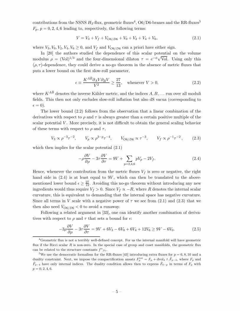
contributions from the NSNS H3-flux, geometric fluxes4, O6/D6-branes and the RR-fluxes5

Fp, p = 0, 2, 4, 6 leading to, respectively, the following terms:

V = V3 + Vf + VO6/D6 + V0 + V2 + V4 + V6, (2.1)

where V3, V0, V2, V4, V6 ≥ 0, and Vf and VO6/D6 can a priori have either sign.

In [20] the authors studied the dependence of this scalar potential on the volume

modulus ρ = (Vol)1/3 and the four-dimensional dilaton τ = e−φ√

Vol. Using only this

(ρ, τ)-dependence, they could derive a no-go theorem in the absence of metric fluxes that

puts a lower bound on the first slow-roll parameter,

ǫ ≡ KAB∂AV ∂BV

V 2≥ 27

13, whenever V > 0, (2.2)

where KAB denotes the inverse Kahler metric, and the indices A,B, . . . run over all moduli

fields. This then not only excludes slow-roll inflation but also dS vacua (corresponding to

ǫ = 0).

The lower bound (2.2) follows from the observation that a linear combination of the

derivatives with respect to ρ and τ is always greater than a certain positive multiple of the

scalar potential V . More precisely, it is not difficult to obtain the general scaling behavior

of these terms with respect to ρ and τ ,

V3 ∝ ρ−3τ−2, Vp ∝ ρ3−pτ−4, VO6/D6 ∝ τ−3, Vf ∝ ρ−1τ−2 , (2.3)

which then implies for the scalar potential (2.1)

−ρ∂V

∂ρ− 3τ

∂V

∂τ= 9V +

∑

p=2,4,6

pVp − 2Vf . (2.4)

Hence, whenever the contribution from the metric fluxes Vf is zero or negative, the right

hand side in (2.4) is at least equal to 9V , which can then be translated to the above-

mentioned lower bound ǫ ≥ 2713 . Avoiding this no-go theorem without introducing any new

ingredients would thus require Vf > 0. Since Vf ∝ −R, where R denotes the internal scalar

curvature, this is equivalent to demanding that the internal space has negative curvature.

Since all terms in V scale with a negative power of τ we see from (2.1) and (2.3) that we

then also need VO6/D6 < 0 to avoid a runaway.

Following a related argument in [33], one can identify another combination of deriva-

tives with respect to ρ and τ that sets a bound for ǫ:

−3ρ∂V

∂ρ− 3τ

∂V

∂τ= 9V + 6V3 − 6V0 + 6V4 + 12V6 ≥ 9V − 6V0. (2.5)

4Geometric flux is not a terribly well-defined concept. For us the internal manifold will have geometric

flux if the Ricci scalar R is non-zero. In the special case of group and coset manifolds, the geometric flux

can be related to the structure constants fαβγ .

5We use the democratic formalism for the RR-fluxes [43] introducing extra fluxes for p = 6, 8, 10 and a

duality constraint. Next, we impose the compactification ansatz F totp = Fp + dvol4 ∧ Fp−4, where Fp and

Fp−4 have only internal indices. The duality condition allows then to express F6−p in terms of Fp with

p = 0, 2, 4, 6.

– 5 –

In the case of vanishing mass parameter, we have V0 = 0, and (2.5) implies ǫ ≥ 97 . Therefore,

we need to have Vf > 0, VO6/D6 < 0 and V0 6= 0 in order to avoid the above no-go theorems.

Note that the only real restriction here is that we have to have a compact space with

negative curvature since we are always free to turn on F0-flux and to do an orientifold

projection. Of the coset models discussed in [40] only the G2

SU(3) case has positive curvature

over the whole parameter space and is thus ruled out by the above no-go theorem. The

other coset spaces studied in [40], on the other hand, do allow for negative curvature and are

thus not affected by the no-go theorem of [20]. This was already noted in [40] and justifies a

closer look at these models. As already mentioned in the introduction we will also discuss

two more coset spaces not analyzed in [40], which do not admit a supersymmetric AdS

vacuum.

3. SU(3)-structure manifolds and a different no-go theorem

The no-go theorems described in the previous section are very general in the sense that

they do not assume anything specific about the geometry of the internal manifold apart

from the possible presence of geometric fluxes, p-form fluxes and O6/D6-brane sources.

An obvious way around the no-go theorem is to look at internal spaces with geometric

fluxes leading to negative curvature. In this section we will use the technology of SU(3)-

structures and discuss a refined no-go theorem [41] that holds for an important subclass of

compactifications with geometric fluxes.

On manifolds with SU(3)-structure, the structure group of the tangent bundle can be

reduced to SU(3), which implies the existence of a non-vanishing, globally defined spinor

field η+.6 In type II compactifications, the effective 4D theory can then be described by

an N = 2 supergravity Lagrangian, which, under suitable orientifold projections, turns

into an effective N = 1 theory. From bilinears of the spinor field one can form a globally

defined real two-form, J , and a complex decomposable three-form, Ω, which generalize,

respectively, the Kahler form and the holomorphic three-form of a Calabi-Yau manifold:7

Jmn = iη†+γmnη+, Ωmnp = η†−γmnpη+, (3.1)

where η− is the complex conjugate of η+, and γmn, etc. denote the weighted antisym-

metrized products of (internal) gamma matrices. Fierz identities then imply

Ω ∧ J =0 , (3.2)

Ω ∧ Ω∗ =4i

3J3 6= 0, (3.3)

6There are more general ways one can decompose the 10D spinor fields into 6D and 4D spinors such

that one still has a 4D N = 2 (or after orientifolding N = 1) supergravity theory. These lead to so-called

SU(3)×SU(3)-structure and the low-energy supergravity is discussed in [44, 45, 46, 48].7On Calabi-Yau manifolds, the spinor field η+ is covariantly constant with respect to the Levi-Civita

connection, implying dJ = dΩ = 0. In our case however, we have generically dJ 6= 0 and dΩ 6= 0, and the

decomposition of these quantities in terms of SU(3)-representations defines the intrinsic torsion classes [21]

(see also [30] for a review). These torsion classes then lead to a non-vanishing curvature scalar and can

thus be related to the geometric flux.

– 6 –

and the 6D volume-form is

dvol6 =1

6J3 = − i

8Ω ∧ Ω∗ . (3.4)

In our concrete models, we will introduce a configuration of O6-planes such that the

resulting low-energy theory in four dimensions is N = 1 supersymmetric. In order not to

be projected out, H,F2 and F6 should be odd, and F0 and F4 should be even under each

orientifold involution. Furthermore, the condition that the orientifold projection does not

fully break the supersymmetry requires J and ReΩ to be odd, and ImΩ to be even under

each orientifold involution. The holomorphic variables of the low-energy N = 1 theory sit

then in the expansion of the complex combinations Jc = J − iδB and Ωc = e−ΦImΩ+ iδC3

[24], where δB and δC3 are fluctuations around the background of the NSNS two-form and

RR three-form potential, respectively, and Φ is the 10D dilaton.

Just as in Calabi-Yau compactifications, one tries to expand the complexified Jc and

Ωc in a suitable basis of forms to yield an analogue of Kahler moduli, ki, and complex

structure moduli uI = τ−1uI :8

Jc =(ki − ibi)Y(2−)i ≡ tiY

(2−)i , (i = 1, . . . , h2−) , (3.5a)

Ωc =(uI + icI)Y(3+)I ≡ zIY

(3+)I , (I = 1, . . . , h3+) . (3.5b)

Here, Y(2−)i and Y

(3+)I are a set of expansion forms with suitable parity under the orientifold

involution, as indicated by the superscript +/−. In contrast to the Calabi-Yau case, they

are in general not harmonic, since Jc and Ωc are not necessarily closed. The numbers h2−

and h3+ therefore do not count harmonic forms and should not be confused with the Hodge

numbers. The easiest way to satisfy the compatibility condition (3.2) is to impose it for

all choices of the moduli ti and zI , which implies for our basis forms

Y(2−)i ∧ Y

(3±)I = 0 , (3.6)

for all i and I.

As the expansion forms are in general not harmonic, the corresponding 4D scalars ti, zI

are usually not massless. There is thus no clear separation into massive and massless modes

as in conventional Calabi-Yau compactifications, and the identification of a suitable expan-

sion basis is generally an important open problem. One approach is to derive constraints

on the basis from the requirement of obtaining an effective supergravity Lagrangian with

an appropriate amount of supersymmetry (N = 2, or N = 1 after orientifolding). Another

would be to find a consistent truncation, and a third, perhaps most physical, would be to

try to establish a hierarchy of masses and keep only the light fields. See [23, 24, 44, 26, 25]

for various approaches to this problem. The position adopted in [40] is that on group man-

ifolds or coset spaces, at least, a natural expansion basis is provided by the left-invariant

forms. In our concrete examples we will restrict our discussions to these cases and hence

8Note that there are h3+ moduli zI whose real parts RezI = uI depend on τ and the (h3+ − 1)

complex structure moduli. We can take out the τ -dependence and define uI = τ uI . So strictly speaking

the uI , I = 1, . . . , h3+ are not the complex structure moduli but rather functions of the (h3+ − 1) complex

structure moduli that are not all independent.

– 7 –

only consider SU(3)-structures that are likewise left-invariant. As expansion forms we will

then choose for Y(2−)i the left-invariant odd two-forms and for Y

(3+)I the left-invariant even

three-forms. In the concrete models of section 4 there are either no odd left-invariant five

forms or we will arrange for them to be projected out by orientifolding, so that the extra

condition (3.6) is trivial.

3.1 The scalar potential in SU(3)-structure compactifications

The main idea of the no-go theorems discussed in section 2 is to find a subset of the moduli

along which the first derivatives of the scalar potential cannot be simultaneously made

sufficiently small for slow-roll inflation. In section 2, the relevant subset of the moduli

consists of the overall volume modulus ρ and the 4D dilaton τ .

We will now closely follow [41] and discuss another no-go theorem that is very similar

in spirit, but concerns a different two-dimensional slice in moduli space that no longer

involves the overall volume ρ, but a different (albeit related) Kahler modulus. In order to

write down the dependence of the scalar potential on the moduli, we first define the Kahler

potential [24]9

K = Kk + Kc + 3 ln(8κ210M

2P ) , (3.7)

where Kk and Kc are the parts containing, respectively, the Kahler and complex struc-

ture/dilaton moduli. They are given by

Kk = − ln

∫

M

4

3J3 = − ln (8Vol) , (3.8a)

Kc = − 2 ln

∫

M2 e−ΦImΩ ∧ e−ΦReΩ = −4 ln τ + Kc , (3.8b)

where Kc only depends on the complex structure moduli uI of footnote 8. Also in the

second line, e−ΦReΩ should be considered as a function of e−ΦImΩ.10 Furthermore, from

the relation (3.4) we find

Vol =e−Kk

8=

κijkkikjkk

6, (3.9)

where κijk denotes the triple intersection number, given in terms of the odd two-forms

Y(2−)i as

κijk =

∫

MY

(2−)i ∧ Y

(2−)j ∧ Y

(2−)k . (3.10)

The Kahler metric is given in the standard way in terms of the Kahler potential11

KIJ =∂2Kk

∂zI∂zJ, Ki =

∂2Kc

∂ti∂t. (3.11)

9The constant last term makes eK dimensionless.10Indeed, e−ΦΩ should be a decomposable form, which, according to [47], implies that one can find

e−ΦReΩ from e−ΦImΩ.11We will use the indices I, J, . . . for both the real coordinates uI as well as the complex coordinates zI .

There should be no confusion as the field itself is always indicated. In the definition of the Kahler metric

the bar-notation emphasizes that the second derivatives is with respect to the complex conjugate. Likewise

for the indices i, j, . . ..

– 8 –

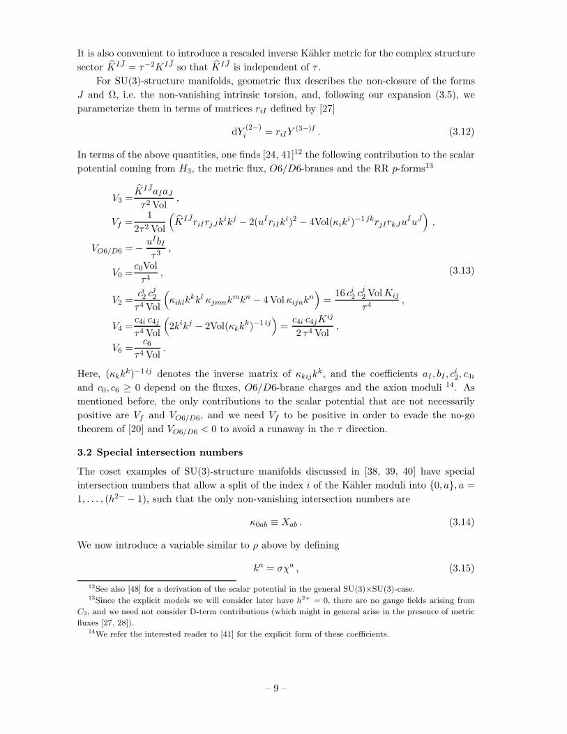
It is also convenient to introduce a rescaled inverse Kahler metric for the complex structure

sector KIJ = τ−2KIJ so that KIJ is independent of τ .

For SU(3)-structure manifolds, geometric flux describes the non-closure of the forms

J and Ω, i.e. the non-vanishing intrinsic torsion, and, following our expansion (3.5), we

parameterize them in terms of matrices riI defined by [27]

dY(2−)i = riIY

(3−)I . (3.12)

In terms of the above quantities, one finds [24, 41]12 the following contribution to the scalar

potential coming from H3, the metric flux, O6/D6-branes and the RR p-forms13

V3 =KIJaIaJ

τ2 Vol,

Vf =1

2τ2 Vol

(KIJriIrjJkikj − 2(uIriIk

i)2 − 4Vol(κiki)−1 jkrjIrkJuIuJ

),

VO6/D6 = − uIbI

τ3,

V0 =c0Vol

τ4,

V2 =ci2 cj

2

τ4 Vol

(κiklk

kkl κjmnkmkn − 4Vol κijnkn)

=16 ci

2 cj2 Vol Ki

τ4,

V4 =c4i c4j

τ4 Vol

(2kikj − 2Vol(κkk

k)−1 ij)

=c4i c4jK

i

2 τ4 Vol,

V6 =c6

τ4 Vol.

(3.13)

Here, (κkkk)−1 ij denotes the inverse matrix of κkijk

k, and the coefficients aI , bI , ci2, c4i

and c0, c6 ≥ 0 depend on the fluxes, O6/D6-brane charges and the axion moduli 14. As

mentioned before, the only contributions to the scalar potential that are not necessarily

positive are Vf and VO6/D6, and we need Vf to be positive in order to evade the no-go

theorem of [20] and VO6/D6 < 0 to avoid a runaway in the τ direction.

3.2 Special intersection numbers

The coset examples of SU(3)-structure manifolds discussed in [38, 39, 40] have special

intersection numbers that allow a split of the index i of the Kahler moduli into 0, a, a =

1, . . . , (h2− − 1), such that the only non-vanishing intersection numbers are

κ0ab ≡ Xab . (3.14)

We now introduce a variable similar to ρ above by defining

ka = σχa , (3.15)

12See also [48] for a derivation of the scalar potential in the general SU(3)×SU(3)-case.13Since the explicit models we will consider later have h2+ = 0, there are no gauge fields arising from

C3, and we need not consider D-term contributions (which might in general arise in the presence of metric

fluxes [27, 28]).14We refer the interested reader to [41] for the explicit form of these coefficients.

– 9 –

where σ is the overall scale of (h2− − 1) Kahler moduli and the χa are constrained by

Xabχaχb = 2. The volume can now simply be written as Vol = k0σ2. We can then write

V2 and V4 in terms of Xab rather than κijk and spell out the explicit dependence on k0 and

σ:

V2 =4

τ4k0σ2

(c02c

02σ

4 + ca2c

b2(k

0)2σ2(XacχcXbdχ

d − Xab))

,

V4 =2

τ4k0σ2

(c40c40(k

0)2 + c4ac4bσ2(χaχb − X−1ab)

).

(3.16)

It follows from the positivity of the Kahler metric (cf. the corresponding terms in (3.13))

and the orthogonality of k0 and ka that the two terms in V2 and the two terms in V4 above

are all separately positive definite.

3.3 No-go theorems in the (τ, σ)-plane

We will now restrict ourselves to the moduli τ and σ and adapt a no-go theorem from [41]

that applies to all but one of the coset models to be discussed in section 4. To this end, we

first isolate the contributions from σ and τ to the slow-roll parameter ǫ. To identify the

contribution from σ, we use the explicit form of the inverse Kahler metric for the Kahler

moduli [24]

Ki = 2kikj − 4Vol(κkkk)−1 ij. (3.17)

For our special intersection numbers (3.14) we then find

1

4Ki ∂V

∂ki

∂V

∂kj=

(k0 ∂V

∂k0

)2

+1

2

(σ

∂V

∂σ

)2

+

(χaχb

2− X−1ab

)∂V

∂χa

∂V

∂χb, (3.18)

where(

χaχb

2 − X−1ab)

projects to the tangent space of the hyperplane χaXabχb = 2.

The slow-roll parameter ǫ is

ǫ =KAB∂φAV ∂φBV

V 2=

KAB(∂ReφAV ∂ReφBV + ∂ImφAV ∂ImφBV

)

4V 2, (3.19)

so that we have (using the τ -dependence of Kc spelled out in (3.8b))

ǫ ≥ 1

V 2

(1

2

(σ

∂V

∂σ

)2

+1

4

(τ∂V

∂τ

)2)

≥ 1

18V 2

(σ

∂V

∂σ+ 2τ

∂V

∂τ

)2

. (3.20)

Thus, if we can show that

DV ≡ (−σ∂σ − 2τ∂τ )V ≥ 6V, (3.21)

we would have

ǫ ≥ 2 , whenever V > 0 , (3.22)

and slow-roll inflation and dS vacua are excluded.

– 10 –

From (3.13) and (3.16) we obtain, for intersection numbers of special form (3.14),

DV3 =6V3 ,

DVO6 =6VO6 ,

DV0 =6V0 ,

DV2 =6V2 + positive term ,

DV4 =8V4 + positive term ,

DV6 =10V6 ,

(3.23)

so (3.21), and hence ǫ ≥ 2, would follow if also DVf ≥ 6Vf . In [41] it was shown that the

extra condition raI = 0 would ensure that DVf = 6Vf , implying the no-go theorem. In the

coset examples to be discussed in the next section, however, one has raI 6= 0. Therefore,

we will explicitly check for each case separately whether DVf ≥ 6Vf is satisfied or not. In

order to do so, it is convenient to write

Vf =1

2τ2VolU , (3.24)

so that

DVf = 6Vf +1

2τ2VolDU = 6Vf +

1

2τ2Vol(−σ∂σ)U, (3.25)

and the no-go theorem applies if we can show that

−σ∂σU = −ka∂kaU ≥ 0 . (3.26)

Furthermore, if the inequality (3.26) is strictly valid, Minkowski vacua are ruled out as

well. This can be seen as follows. Using (3.23) and (3.25), we obtain

DV = 6V + 2V4 + 4V6 +1

2τ2Vol(−σ∂σ)U + positive terms , (3.27)

so that for a vacuum, DV = 0, we find with (3.26)

V = −1

6

(2V4 + 4V6 +

1

2τ2Vol(−σ∂σ)U + positive terms

)≤ 0 . (3.28)

So, if the inequality (3.26) holds strictly, also (3.28) holds strictly as well, and Minkowski

vacua are ruled out.

Indeed, we checked in particular that the coset models of section 4 do not allow for

supersymmetric Minkowski vacua with left-invariant SU(3)-structure. Strangely enough,

this includes the case SU(2)×SU(2) for which eq. (3.26) can be violated. This model may

still allow for a non-supersymmetric Minkowski vacuum. Incidentally, we checked also that

there are no supersymmetric Minkowski vacua on any of the cosets of table 1 with static

SU(2)-structure, which falls outside the scope of the SU(3)-structure based no-go theorem

of this section.

– 11 –

3.4 A comment on extra ingredients

Some ingredients that are not taken into account in the original no-go theorem of [20],

nor in the no-go theorems of section 3.3 are KK-monopoles, NS5-branes, D4-branes and

D8-branes. Some of these ingredients were used in constructing simple dS-vacua in [31].

KK-monopoles would drastically change the topology and geometry of the internal manifold

so that their introduction makes it difficult to obtain a clear ten-dimensional picture, hence

we will not discuss this possibility further in this paper. NS5-branes, D4-branes and D8-

branes would contribute through their respective currents jNS5, jD4 and jD8 as follows to

the Bianchi identities

dH = −jNS5 ,

dF4 + H ∧ F2 = −jD4 ,

dF0 = −jD8 .

(3.29)

Since H and F2 should be odd, and F0 and F4 even under all the orientifold involutions, we

find that jNS5 is an odd four-form, jD4 an even five-form and jD8 an even one-form. In the

approximation of left-invariant SU(3)-structure to be used in the next section, one should

also impose these brane-currents to be left-invariant (making the branes itself smeared

branes). For the concrete models of section 4 there are no such currents jNS5, jD4 or jD8

with the appropriate properties under all orientifold involutions, implying that NS5-branes,

D4- and D8-branes cannot be used in these models.

Let us briefly mention that an F-term uplifting along the lines of O’KKLT [49, 50]

by combining the coset models with the quantum corrected O’Raifeartaigh model will not

be a promising possibility either. The O’Raifeartaigh model is given by WO = −µ2S and

KO = SS − (SS)2

Λ2 . The model has a dS minimum for S = 0 where VO ≈ µ4. We combine

the two models as follows (the subscript IIA refers to the previously discussed flux and

brane contributions)

W = WIIA + WO , K = KIIA + KO . (3.30)

In lowest order in S the total potential is then given by

V ≈ VIIA + eKIIAVO + . . . . (3.31)

Note that we can then include the contribution of Vup = eKIIAVO in the no-go theorems,

because the uplift potential Vup scales like F6,

Vup =Aup

τ4 Vol. (3.32)

Since we assume a positive uplift potential, Vup > 0, the fact that Vup scales like F6 tells

us that adding this uplift potential does not help in circumventing the no-go theorems of

section 2 or section 3.3.

– 12 –

4. Application: coset models

In the previous section, we described a no-go theorem that rules out dS vacua and slow-

roll inflation for type IIA compactifications on certain types of SU(3)-structure manifolds,

namely those for which one coordinate in the triple intersection number κijk can be sepa-

rated as in eq. (3.14) and the geometric fluxes induce the relation (3.26). While these seem

to be quite strong assumptions, it turns out that a large part of the explicitly known ex-

amples of non-trivial SU(3)-structure compactifications actually do fall into this category,

as we will show in this section.

As a starting point we could consider internal manifolds, for which an explicit SU(3)-

structure compactification to a supersymmetric AdS space-time is known [40]. We are not

directly interested in this AdS vacuum, but the moduli space of such a compactification

might still have regions where the scalar potential is positive and allows for local dS minima

or suitable inflationary trajectories. The explicitly known models with supersymmetric AdS

vacua can be divided into two classes:

• Nilmanifolds (or “twisted tori”)15

• Group manifolds and coset spaces based on semi-simple and U(1)-groups

In each case, only left-invariant SU(3)-structures are considered. The scalar curvature of

a nilmanifold reads R = −14fγ1

α1β1fγ2

α2β2gγ1γ2

gα1α2gβ1β2 in terms of the internal metric

gαβ and the structure constants fγαβ of the nilpotent group. Apart from the torus, this is

always negative so that, as discussed in section 2, the nilmanifolds provide prime candidates

for avoiding the no-go theorem of [20]. However, the only known nilmanifold example, next

to the torus, allowing for an N = 1 AdS4 solution is the Iwasawa manifold, which turns

out to be T-dual to the torus solution [52, 40]. Having no geometric fluxes, the torus is

ruled out by the no-go theorem of [20], and one expects this to be true then also for the

Iwasawa manifold because of T-duality.

The second class of explicitly known examples, i.e. the group manifolds and coset spaces

based on semi-simple and U(1)-groups, will in the following simply be referred to as “the

coset models”. For reviews on coset spaces see [53, 54]. As was explained in [39], in order

for a coset space G/H to allow for an SU(3)-structure, the group H should be contained in

SU(3).16 The list of such six-dimensional cosets and the corresponding structure constants

were given in [39] and are summarized in table 1. Out of these only five lead to N = 1

AdS4 solutions [39], as we have indicated in the table. In [40], the low-energy effective

actions for these compactifications were calculated, so we can now check whether the no-go

theorems described above can be applied.

For the cosmological applications we have in mind, however, it is not really relevant

whether the effective field theories actually have supersymmetric vacua. All we are re-

ally interested in here are regions in moduli space with positive potential energy, where15Nilmanifolds are group manifolds of nilpotent groups, quotiented by a discrete group to make them

compact. In the physics literature they are known as twisted tori, since they can be described as torus

bundles on tori. See [51] for a short introduction.16These coset spaces were already considered in the construction of heterotic string compactifications by

[55].

– 13 –

G H N = 1 AdS4

G2 SU(3) Yes

SU(3)×SU(2)2 SU(3) No

Sp(2) S(U(2)×U(1)) Yes

SU(3)×U(1)2 S(U(2)×U(1)) No

SU(2)3×U(1) S(U(2)×U(1)) No

SU(3) U(1)×U(1) Yes

SU(2)2×U(1)2 U(1)×U(1) No

SU(3)×U(1) SU(2) Yes

SU(2)3 SU(2) No

SU(2)2×U(1) U(1) No

SU(2)2 1 Yes

Table 1: All six-dimensional manifolds of the type M = G/H , where H is a subgroup of SU(3)

and G and H are both products of semi-simple and U(1)-groups. To be precise this list should be

completed with the cosets obtained by replacing any number of SU(2) factors in G by U(1)3.

supersymmetry is spontaneously broken anyway. It is thus interesting to consider also

compactifications that do not allow for supersymmetric AdS vacua. Still restricting to

left-invariant SU(3)-structure there are only two more coset spaces of table 1. They areSU(2)2

U(1) × U(1) and SU(2)×U(1)3.

In this section we will study each of these coset models separately, i.e. the seven

models that allow for a left-invariant SU(3)-structure (including the five that also allow for

a supersymmetric AdS vacuum). For the first four models the condition of left-invariance

is very strong, and leaves only a very limited set of two-forms and three-forms as expansion

forms, while there are no left-invariant one-forms nor five-forms. In these cases, we are able

to show the no-go theorem without assuming that we introduce orientifolds. In the models

with G = SU(2)2

U(1) ×U(1), SU(2)×U(1)3 and SU(2)×SU(2) there are left-invariant one-forms

and five-forms, which complicates matters. For instance, the condition (3.6) becomes

non-trivial. So in each of these cases, we will introduce enough orientifolds to eliminate

one- and five-forms. Furthermore, we will make the simplification that the orientifolds

are perpendicular to the coordinate frame, except for SU(2)×SU(2), which does not allow

for perpendicular orientifolds. It turns out that in that case one can choose the same

orientifolds as in the supersymmetric AdS vacua of [40] leading to the same expansion

forms.

As we will show, dS vacua (as well as Minkowski) and slow-roll inflation are excluded

for all these coset cases by the no-go theorem (3.26), except for the case SU(2)×SU(2).

Not requiring the presence of a supersymmetric SU(3)-structure AdS vacuum, one can

consider, next to the nilmanifolds, also the solvmanifolds i.e. the group manifolds of a

solvable Lie group (for related work see [33]). Without the additional conditions on the

left invariance as for cosets, both nilmanifolds and solvmanifolds will however also allow

– 14 –

for one- and five-forms, and a large amount of fields. A detailed study of all cases would

probably also require considering different choices of orientifolds on each manifold, and we

leave this for future work.

4.1 Models for which the no-go theorems hold

4.1.1 G2

SU(3)

For this case, one finds for the function U of (3.24):

U ∝ −(k1)2 , (4.1)

which is manifestly negative. This implies that Vf itself is manifestly negative so that the

no-go theorem of [20], reviewed in section 2, already rules out this case [40]. All other

coset models allow for values of the moduli such that Vf > 0 and therefore require a more

careful analysis using the refined no-go theorem of section 3.3.

4.1.2 Sp(2)S(U(2)×U(1))

For this case, one has

U ∝ (k2)2 − 4(k1)2 − 12k1k2 , (4.2)

and the only non-vanishing intersection number is κ112 and permutations thereof, so that

k2 plays the role of k0, and we have

DU = −k1∂k1U ∝ 8(k1)2 + 12k1k2 > 0 , (4.3)

so that with ki > 0 (because of metric positivity) the inequality (3.26) is strictly satisfied

and this model is ruled out.

4.1.3 SU(3)U(1)×U(1)

For this coset space, we have

U ∝ (k1)2 + (k2)2 + (k3)2 − 6k1k2 − 6k2k3 − 6k1k3 , (4.4)

and the non-vanishing intersection numbers are of the type κ123 so that we can choose any

one of the three k’s as k0. We will choose k0 to be the biggest and assume without loss of

generality that this is k1, i.e. that k1 ≥ k2, k3. We then find that

DU = (−k2∂k2 − k3∂k3)U ∝ (6k1 − 2k2)k2 + (6k1 − 2k3)k3 + 12k2k3 > 0, (4.5)

so that with ki > 0 (because of metric positivity) this coset space is also ruled out by the

no-go theorem (3.26).

– 15 –

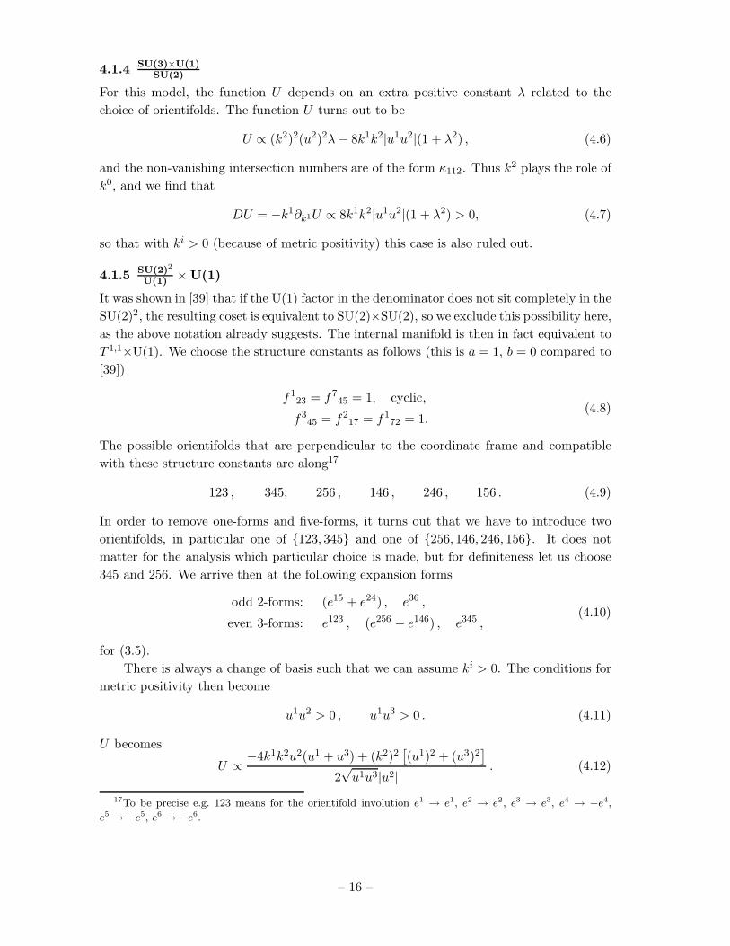
4.1.4 SU(3)×U(1)SU(2)

For this model, the function U depends on an extra positive constant λ related to the

choice of orientifolds. The function U turns out to be

U ∝ (k2)2(u2)2λ − 8k1k2|u1u2|(1 + λ2) , (4.6)

and the non-vanishing intersection numbers are of the form κ112. Thus k2 plays the role of

k0, and we find that

DU = −k1∂k1U ∝ 8k1k2|u1u2|(1 + λ2) > 0, (4.7)

so that with ki > 0 (because of metric positivity) this case is also ruled out.

4.1.5 SU(2)2

U(1) × U(1)

It was shown in [39] that if the U(1) factor in the denominator does not sit completely in the

SU(2)2, the resulting coset is equivalent to SU(2)×SU(2), so we exclude this possibility here,

as the above notation already suggests. The internal manifold is then in fact equivalent to

T 1,1×U(1). We choose the structure constants as follows (this is a = 1, b = 0 compared to

[39])

f123 = f7

45 = 1, cyclic,

f345 = f2

17 = f172 = 1.

(4.8)

The possible orientifolds that are perpendicular to the coordinate frame and compatible

with these structure constants are along17

123 , 345, 256 , 146 , 246 , 156 . (4.9)

In order to remove one-forms and five-forms, it turns out that we have to introduce two

orientifolds, in particular one of 123, 345 and one of 256, 146, 246, 156. It does not

matter for the analysis which particular choice is made, but for definiteness let us choose

345 and 256. We arrive then at the following expansion forms

odd 2-forms: (e15 + e24) , e36 ,

even 3-forms: e123 , (e256 − e146) , e345 ,(4.10)

for (3.5).

There is always a change of basis such that we can assume ki > 0. The conditions for

metric positivity then become

u1u2 > 0 , u1u3 > 0 . (4.11)

U becomes

U ∝ −4k1k2u2(u1 + u3) + (k2)2[(u1)2 + (u3)2

]

2√

u1u3|u2|. (4.12)

17To be precise e.g. 123 means for the orientifold involution e1 → e1, e2 → e2, e3 → e3, e4 → −e4,

e5 → −e5, e6 → −e6.

– 16 –

The non-vanishing intersection number is κ112 so that k2 plays the role of k0, and we get

for (3.26):

DU = −k1∂k1U ∝ 2k1k2u2(u1 + u3)√u1u3|u2|

> 0 , (4.13)

which is positive using the conditions (4.11). Hence, this case is ruled out as well.

4.1.6 SU(2)×U(1)3

In this case there are ten possible orientifold planes perpendicular to the coordinate frame

and compatible with the structure constants. It turns out that in order to remove the one-

and five-forms we have to choose at least three mutually supersymmetric orientifolds and

that it does not matter for the analysis which ones we choose. For definiteness, let us take

123 , 356, 246 . (4.14)

With these orientifolds, we get the following expansion forms to be used in (3.5)

odd 2-forms: e16 , e25 , e34 ,

even 3-forms: e123 , e356 , e264 , e145 .(4.15)

Again there is always a change of basis such that we can assume ki > 0. The positivity of

the metric demands that

u1u2 > 0 , u1u3 > 0 , u1u4 > 0 . (4.16)

For the quantity U as defined in (3.24) we get

U ∝ (k1u4)2 + (k2u3)2 + (k3u2)2 − 2k1u4k2u3 − 2k1u4k3u2 − 2k2u3k3u2

2√

u1u2u3u4. (4.17)

The non-vanishing intersection number is κ123 so that each ki can play the role of k0.

Without loss of generality we can assume k1u4 ≥ k2u3 > 0, k1u4 ≥ k3u2 > 0 and choose

k0 to be k1. Thus we then find

DU = (−k2∂k2 − k3∂k3)U ∝ −(k2u3 − k3u2)2 + k1u4(k2u3 + k3u2)√u1u2u3u4

> 0 , (4.18)

so that we can also rule out this model.

4.2 SU(2) × SU(2)

Thus far, we have found that ǫ ≥ 2 for all other cases. For the remaining coset space

SU(2)×SU(2), one finds

U ∝3∑

i=1

(ki)2

(4∑

I=1

(uI)2

)− 4k2k3(|u1u2| + |u3u4|)

− 4k1k2(|u1u4| + |u2u3|) − 4k1k3(|u1u3| + |u2u4|

),

(4.19)

and the non-vanishing intersection numbers are of the form κ123 so that we could choose

any one of the k’s as k0. However, it is not possible to apply the no-go theorem. This

can be easily seen if we take for example u1 ≫ u2, u3, u4. Then we have schematically

U ∝ ~k2(u1)2 and DU ∝ −kaka(u1)2 < 0. In [41] further no-go theorems have been derived

but none of those apply to this case either. Let us therefore study it in more detail.

– 17 –

4.2.1 Small ǫ for SU(2) × SU(2)

We have argued above that the known no-go theorems cannot be used to rule out small

ǫ for this compactification. Indeed we will see that ǫ ≈ 0 is possible and there are dS

extrema.

The superpotential and Kahler potential of the effective N = 1 supergravity have

been derived in various ways in [44, 45, 46] (based on earlier work of [56, 23, 24]). Here we

summarize the main formulæ which will be used in the following. The superpotential for

SU(3)-structure reads in the Einstein frame

W =1

4κ210

∫

M〈ei(J−iδB), F − idH

(e−ΦImΩ + iδC3

)〉 , (4.20)

where 〈φ1, φ2〉 = φ1∧λ(φ2)|top is the Mukai pairing. λ is the operator reversing the indices

of a form and |top selects the part of top dimension six, as necessary to integrate over the

internal manifold M . The scalar potential is given in terms of the superpotential via

V (φ, φ) = M−2p eK

(KABDAWDBW∗ − 3|W|2

). (4.21)

In order to eliminate the one- and five-forms we must introduce at least three mutually

supersymmetric orientifolds, compatible with the structure constants. We can then always

perform a basis transformation so that the odd two-forms and odd/even three-forms are

the same as in [40] and read18

Y(2−)1 =e14, Y

(2−)2 = e25, Y

(2−)3 = e36,

Y (3−)1 =1

4

(e156 − e234 − e246 + e135 + e345 − e126 + e123 − e456

),

Y (3−)2 =1

4

(e156 − e234 + e246 − e135 − e345 + e126 + e123 − e456

),

Y (3−)3 =1

4

(e156 − e234 + e246 − e135 + e345 − e126 − e123 + e456

),

Y (3−)4 =1

4

(−e156 + e234 + e246 − e135 + e345 − e126 + e123 − e456

),

Y(3+)1 =

1

2

(e156 + e234 − e246 − e135 + e345 + e126 + e123 + e456

),

Y(3+)2 =

1

2

(e156 + e234 + e246 + e135 − e345 − e126 + e123 + e456

),

Y(3+)3 =

1

2

(e156 + e234 + e246 + e135 + e345 + e126 − e123 − e456

),

Y(3+)4 =

1

2

(−e156 − e234 + e246 + e135 + e345 + e126 + e123 + e456

),

(4.22)

where the eα (α = 1, . . . , 6) are a basis of left-invariant 1-forms, and we use the shorthand

notation e14 = e1 ∧ e4 etc. The eα satisfy

deα = −1

2fα

βγeβ ∧ eγ , (4.23)

18There are no even two-forms for our choice of orientifold involutions.

– 18 –

where the structure constants for SU(2) × SU(2) are f123 = f4

56 = 1, cyclic19. From this

we find

dY(2−)i = riIY

(3−)I , with r =

1 1 1 −1

1 −1 −1 −1

1 −1 1 1

. (4.24)

In terms of the above expansion forms, we can again define the complex moduli as in (3.5).

The positivity of the metric demands

u1u2 < 0 , u3u4 < 0 , u1u4 < 0 . (4.25)

Next we turn to the choice of background fluxes. As explained in appendix A, for the part

of the moduli space where H is non-trivial in cohomology, p 6= 0 (see below), the most

general form of the background fluxes is

F0 =m, (4.26a)

F2 =miY(2−)i , (4.26b)

F4 =0, (4.26c)

F6 =0, (4.26d)

H =p(Y

(3−)1 + Y

(3−)2 − Y

(3−)3 + Y

(3−)4

). (4.26e)

Plugging in these background values for the fluxes together with the expansion (3.5) in

terms of the basis (4.22), we find for the superpotential (4.20)

W = Vs(4κ210)

−1(m1t2t3 + m2t1t3 + m3t1t2 − imt1t2t3 − ip(z1 + z2 − z3 + z4) + riIt

izI)

,

(4.27)

and the Kahler potential

K = − ln

3∏

i=1

(ti + ti

)− ln

4∏

I=1

(zI + zI

)+ 3 ln

(V −1

s κ210M

2P

)+ ln 32 , (4.28)

where Vs = −∫M e123456. Note that the superpotential depends on all the moduli so there

are no flat directions in this model.

It is straightforward to calculate the scalar potential (4.21) and the slow-roll parameter

ǫ from the Kahler and superpotential. Although we cannot analytically minimize ǫ, we can

do it numerically. One particular solution with numerically vanishing ǫ is

m1 = m2 = m3 = L , m = 2L−1 , p = 3L2 ,

k1 = k2 = k3 ≈ .8974L2 , b1 = b2 = b3 ≈ −.8167L2 ,

u1 ≈ 2.496L3, u2 = −u3 = u4 ≈ −.05667L3 ,

c1 ≈ −2.574L3 , c2 = −c3 = c4 ≈ .3935L3 ,

(4.29)

19This model can be thought of as a twisted version of T 6/(Z2 × Z2) as discussed in [37]. In that paper

the authors focused on moduli stabilization and model building while we are interested in the cosmological

aspects.

– 19 –

where L is an arbitrary length. While we can use L to scale up our solution with respect

to the string length ls, we stress that this does not correspond to a massless modulus, as

it also changes the fluxes.

We conclude that in this case there is no lower bound for ǫ. To obtain a trustworthy

supergravity solution we would have to make sure that the internal space is large compared

to the string length and that the string coupling is small (for which we could use our freedom

in L). Furthermore, in the full string theory the fluxes have to be properly quantized.

Although we do not think that this would prevent small ǫ, we did not try to find such a

solution because all the solutions with vanishing ǫ we found have a more serious problem,

namely that η . −2.4. The eigenvalues of the mass matrix turn out to be generically all

positive except for one, with the one tachyonic direction being a mixture of all the light

fields, in particular the axions. This means that we have a saddle point rather than a dS

minimum. A similar instability was found in related models in [41].

In [42], a no-go theorem preventing dS vacua and slow-roll inflation was derived by

studying the eigenvalues of the mass matrix. Allowing for an arbitrary tuning of the

superpotential it was shown that for certain Kahler potentials the Goldstino mass is always

negative. For the examples we found, this mass is always positive so that the no-go theorem

of [42] does not apply. This means that allowing for an arbitrary superpotential it should

be possible to remove the tachyonic direction. In our case, however, the superpotential is

of course not arbitrary.

Since the no-go theorems against slow-roll inflation do not apply and we have found

solutions with vanishing ǫ, we checked whether our solutions allow for small η in the vicinity

of the dS extrema. Unfortunately, this is not the case. In fact, we found that η does not

change much in the vicinity of our solutions where ǫ is still small.

It would be very interesting to study the SU(2)×SU(2) model further to check whether

one can prove that there is always at least one tachyonic direction or whether it allows for

metastable dS vacua after all. Understanding this tachyonic direction better should also

allow to decide whether there are points in the moduli space that allow for slow-roll inflation

in this model.

5. Conclusions and outlook

Type IIA compactifications on orientifolds of SU(3)-structure manifolds with fluxes and

D6-branes are phenomenologically interesting because they lead to effective 4D N = 1

supergravity actions with rich potentials for the moduli. These potentials have a dilaton-

volume dependence that forbids dS vacua or slow-roll inflation unless the compact space

has a negative scalar curvature induced by the geometric fluxes (or other more complex

ingredients are introduced [20, 31, 33]).

Motivated by this, we analysed a class of explicitly known SU(3)-structure compacti-

fications with fluxes and O6/D6-sources for which the full scalar potential can be written

down in closed form. The manifolds we studied are those coset spaces or group manifolds

based on semi-simple and U(1) groups that admit a left-invariant SU(3)-structure [39].

– 20 –

As indicated in table 1, five out of these seven manifolds allow for 4D N = 1 AdS

solutions that solve the full 10D field equations of massive IIA supergravity [39]. Apart

from a particular nilmanifold (the Iwasawa manifold) and tori, these are, to the authors

best knowledge, the only explicitly known examples of this type. Using the 4D effective

action worked out in [40], we could rule out dS (as well as Minkowski) vacua and slow-

roll inflation elsewhere in moduli space for four of these coset spaces by using a refined

no-go theorem that probes the scalar potential also along a Kahler modulus different from

the overall volume modulus (see also [41]). Just as the no-go theorem of [20], this no-go

theorem works by establishing a certain lower bound on the first derivatives of the potential,

and hence the epsilon parameter, for V ≥ 0. It is thus different in spirit from the no-go

theorems given in [42], which assume a small first derivative and consider consequences for

the second derivatives, i.e. the eta parameter.

The only coset space that allows for supersymmetric vacua and that is not directly

ruled out by any known no-go theorem is then the group manifold SU(2)×SU(2). For this

case, we were indeed able to find critical points (corresponding to numerically vanishing ǫ)

with positive energy density, but only at the price of a tachyonic direction, corresponding

to a large negative eta-parameter, η . −2.4. Interestingly, this tachyonic direction does not

correspond to the one used in the different types of no-go theorems of [42]. As our numerical

search was not exhaustive, however, we cannot completely rule out the existence of dS vacua

or inflating regions for this case. Since this case also does not allow for a supersymmetric

Minkowski vacuum as mentioned below (3.28), our discussion covers all SU(3)-structure

compactifications on semi-simple and U(1) cosets that have a supersymmetric vacuum.

Furthermore, we also studied the remaining two coset spaces of table 1 that do admit

an SU(3)-structure but no supersymmetric AdS vacuum. Choosing for simplicity the O-

planes such that one-forms are projected out and restricting to O-planes perpendicular to

the coordinate frame, we could again use the refined no-go theorem of section 3.3 to rule

out dS vacua and slow-roll inflation for both of these cases as well.

Our results show that a negative scalar curvature and a non-vanishing F0 is in general

not enough to ensure dS vacua or inflation (as also noted in [33]), and we give a geometric

criterion that allows one to separate interesting SU(3)-structure compactifications from

non-realistic ones.

Our study could be extended in several directions. For one thing, it would be extremely

interesting to find explicit SU(3)-structure manifolds that do not fall under the class of

coset spaces we have discussed here and to investigate their usefulness for cosmological

applications along the lines of this paper. The most obvious class of manifolds to study

systematically would be the nil- and solvmanifolds. Another interesting direction might be

the study of compactifications on manifolds with N = 1 spinor ansatze more general than

the SU(3)-structure case [57]. Concerning the SU(2)×SU(2) model discussed in our paper,

one might try to either find a working dS minimum, or rule it out based on another no-go

theorem, perhaps by using methods similar in spirit to [42], although a direct application of

their results to this case does not seem possible. Following [31, 32] or [58, 59, 60], one could

also try to incorporate additional structures such as NS5-branes or quantum corrections of

various types. In section 3.4, however, we found that at least for our models, the following

– 21 –

additional ingredients cannot be added or do not work: NS5-, D4- and D8-branes as well

as an F-term uplift along the lines of O’KKLT [49, 50]. Perhaps also methods similar to

the ones in [61] for non-supersymmetric Minkowski or AdS vacua might be useful for the

direct 10D construction of dS compactifications. There is certainly a lot to improve about

our understanding of cosmologically realistic compactifications of the type IIA string!

Acknowledgments

We would like to thank Davide Cassani, Thomas Grimm, Jan Louis, Luca Martucci, Erik

Plauschinn, Dimitrios Tsimpis, Alexander Westphal, and in particular Raphael Flauger,

Sonia Paban and Daniel Robbins for useful discussions and correspondence. This work is

supported by the Transregional Collaborative Research Centre TR33 “The Dark Universe”

and the Excellence Cluster “The Origin and the Structure of the Universe” in Munich.

C. C., P. K., T. W. and M. Z. are supported by the German Research Foundation (DFG)

within the Emmy-Noether-Program (Grant number ZA 279/1-2).

A. Labelling the disconnected bubbles of moduli space by flux quanta

In section 4.2 we will search for a configuration with small ǫ somewhere in the moduli

space. As we will argue in a moment, this moduli space consists of different disconnected

“bubbles”, i.e. these bubbles are such that it is not possible to reach another bubble by finite

fluctuations of the moduli fields. The approach of [40] of starting from a supersymmetric

configuration and expanding around it is inadequate for studying the whole configuration

space since on the one hand, there will be bubbles that do not contain a supersymmetric

configuration, while on the other hand, there are bubbles that contain more than one

supersymmetric configuration. In fact, in section 4.2 we find configurations with ǫ ≈ 0

and V > 0 in bubbles that do not allow for supersymmetric AdS vacua. We follow here

the standard approach of classifying the moduli space by flux quanta, which is however

complicated by the presence of Romans mass, H-field and O6-plane source.

Classifying the different bubbles in terms of fluxes amounts to finding configurations

that solve the Bianchi identities

dH = 0 , (A.1a)

dF0 = 0 , (A.1b)

dF2 + mH = −j3 , (A.1c)

dF4 + H ∧ F2 = 0 , (A.1d)

while two configurations are considered equivalent if they are related by a fluctuation of

the moduli fields, which after imposing the orientifold projection (and assuming it removes

one-forms) is given by [40]

δH = dδB , (A.2a)

δF0 = 0 , (A.2b)

– 22 –

δF2 = −mδB , (A.2c)

δF4 = dδC3 − δB ∧ (F2 + δF2) −1

2m(δB)2 , (A.2d)

δF6 = H ∧ δC3 − δB ∧ (F4 + δF4) −1

2(δB)2 ∧ (F2 + δF2) −

1

3!m(δB)3 . (A.2e)

In other words, we want to find representatives of the cohomology of the Bianchi identities

(A.1) modulo pure fluctuations of the potentials (A.2).

From eqs. (A.1a), (A.1b), (A.2a) and (A.2b) follows immediately that H ∈ H3(M, R)

and F0 constant. To analyse (A.1c) and (A.2c) we take the point of view that we choose

the flux F2, which then determines the source j3. In fact, if F0 6= 0 the flux F2 is only

determined up to a closed form, since the fluctuation δB was from (A.2a) also only deter-

mined up to a closed form, which can then be used in (A.2c). Moving on to F4, we find

that in eq. (A.1d) H∧F2 = 0, since we assumed there were no even five-forms under all the

orientifold involutions. Moreover, with the fluctuations δC3 we can remove the exact part

of F4 so that F4 ∈ H4(M, R). This however, leaves the closed part of δC3 undetermined,

which, if we have chosen H non-trivial, can in the SU(2)×SU(2) case be used to put F6 = 0.

Taking into account the parity requirements under the orientifold involution, we find

for the case of SU(2)×SU(2) the general form of the background eq. (4.26) when H is

non-trivial. If H is trivial one must allow for non-zero F6.

References

[1] E. Komatsu et al. [WMAP Collaboration], “Five-Year Wilkinson Microwave Anisotropy

Probe (WMAP) Observations: Cosmological Interpretation,” arXiv:0803.0547 [astro-ph];

D. N. Spergel et al. [WMAP Collaboration], “Wilkinson Microwave Anisotropy Probe

(WMAP) three year results: Implications for cosmology,” Astrophys. J. Suppl. 170 (2007)

377 [arXiv:astro-ph/0603449].

[2] A. H. Guth, “The inflationary universe: a possible solution to the horizon and flatness

problems,” Phys. Rev. D 23 (1981) 347; A. D. Linde, “A new inflationary universe scenario:

a possible solution of the horizon, flatness, homogeneity, isotropy and primordial monopole

problems,” Phys. Lett. B 108 (1982) 389; A. Albrecht and P. J. Steinhardt, “Cosmology for

grand unified theories with radiatively induced symmetry breaking,” Phys. Rev. Lett. 48

(1982) 1220.

[3] V. Mukhanov, “Physical foundations of cosmology,” Cambridge, UK: Univ. Pr. (2005) 421p;

S. Weinberg, “Cosmology,” Oxford University Press, USA (2008), 544p; A. Linde, “Particle

physics and cosmology,” Haarwood, Chur, Switzerland (1990) [arXiv:hep-th/0503203];

A. R. Liddle, D. H. Lyth “Cosmological inflation and large-scale structure,” Cambridge, UK:

Univ. Pr. (2000) 400p.

[4] A. G. Riess et al. [Supernova Search Team Collaboration], “Observational evidence from

supernovae for an accelerating universe and a cosmological constant,” Astron. J. 116 (1998)

1009 [arXiv:astro-ph/9805201]; S. Perlmutter et al. [Supernova Cosmology Project

Collaboration], “Measurements of Ω and Λ from 42 high-redshift supernovae,” Astrophys. J.

517 (1999) 565 [arXiv:astro-ph/9812133].

– 23 –

[5] S. H. Henry Tye, “Brane inflation: String theory viewed from the cosmos,” Lect. Notes Phys.

737 (2008) 949 [arXiv:hep-th/0610221]; J. M. Cline, “String cosmology,”

arXiv:hep-th/0612129; R. Kallosh, “On Inflation in String Theory,” Lect. Notes Phys. 738

(2008) 119 [arXiv:hep-th/0702059]; A. Linde, “Inflationary Cosmology,” Lect. Notes Phys.

738 (2008) 1 [arXiv:0705.0164 [hep-th]]; C. P. Burgess, “Lectures on Cosmic Inflation and

its Potential Stringy Realizations,” PoS P2GC, 008 (2006) [Class. and Quant. Grav. 24

(2007) S795] [arXiv:0708.2865 [hep-th]]; L. McAllister and E. Silverstein, “String

Cosmology: A Review,” Gen. Rel. Grav. 40 (2008) 565 [arXiv:0710.2951 [hep-th]].

[6] C. Herdeiro, S. Hirano and R. Kallosh, “String theory and hybrid inflation/acceleration,” J.

High Energy Phys. 0112 (2001) 027 [arXiv:hep-th/0110271]; K. Dasgupta, C. Herdeiro,

S. Hirano and R. Kallosh, “D3/D7 inflationary model and M-theory,” Phys. Rev. D 65

(2002) 126002 [arXiv:hep-th/0203019]; K. Dasgupta, J. P. Hsu, R. Kallosh, A. Linde and

M. Zagermann, “D3/D7 brane inflation and semilocal strings,” J. High Energy Phys. 0408

(2004) 030 [arXiv:hep-th/0405247]; M. Haack, R. Kallosh, A. Krause, A. Linde, D. Lust and

M. Zagermann, “Update of D3/D7-Brane Inflation on K3 × T 2/Z2,” Nucl. Phys. B 806

(2009) 103 [arXiv:0804.3961 [hep-th]]; C. P. Burgess, J. M. Cline and M. Postma, “Axionic

D3-D7 Inflation,” arXiv:0811.1503 [hep-th].

[7] S. Kachru, R. Kallosh, A. Linde and S. P. Trivedi, “De Sitter vacua in string theory,” Phys.

Rev. D 68 (2003) 046005 [arXiv:hep-th/0301240].

[8] S. Kachru, R. Kallosh, A. Linde, J. M. Maldacena, L. P. McAllister and S. P. Trivedi,

“Towards inflation in string theory,” JCAP 0310 (2003) 013 [arXiv:hep-th/0308055].

[9] S. B. Giddings, S. Kachru and J. Polchinski, “Hierarchies from fluxes in string

compactifications,” Phys. Rev. D 66 (2002) 106006 [arXiv:hep-th/0105097].

[10] R. Blumenhagen, B. Kors, D. Lust and S. Stieberger, “Four-dimensional string

compactifications with D-branes, orientifolds and fluxes,” Phys. Rept. 445 (2007) 1

[arXiv:hep-th/0610327].

[11] C. Angelantonj and A. Sagnotti, “Open strings,” Phys. Rept. 371 (2002) 1 [Erratum-ibid.

376 (2003) 339] [arXiv:hep-th/0204089]; A. M. Uranga, “Chiral four-dimensional string

compactifications with intersecting D-branes,” Class. and Quant. Grav. 20 (2003) S373

[arXiv:hep-th/0301032]. E. Kiritsis, “D-branes in standard model building, gravity and

cosmology,” Fortschr. Phys. 52 (2004) 200, Phys. Rept. 421 ((2005) 105 [Erratum Phys.

Rept. 429 (2006) 121] [arXiv:hep-th/0310001]; F. G. Marchesano Buznego, “Intersecting

D-brane models,” arXiv:hep-th/0307252; D. Lust, “Intersecting brane worlds: A path to the

standard model?,” Class. and Quant. Grav. 21 (2004) S1399 [arXiv:hep-th/0401156];

R. Blumenhagen, M. Cvetic, P. Langacker and G. Shiu, “Toward realistic intersecting

D-brane models,” Ann. Rev. Nucl. Part. Sci. 55, 71 (2005) [arXiv:hep-th/0502005].

[12] F. Gmeiner and G. Honecker, “Millions of Standard Models on Z′6?,” J. High Energy Phys.

0807 (2008) 052 [arXiv:0806.3039 [hep-th]].

[13] R. Blumenhagen, V. Braun, T. W. Grimm and T. Weigand, “GUTs in type IIB orientifold

compactifications,” arXiv:0811.2936 [hep-th].

[14] R. Donagi and M. Wijnholt, “Model building with F-Theory,” arXiv:0802.2969 [hep-th];

C. Beasley, J. J. Heckman and C. Vafa, “GUTs and Exceptional Branes in F-theory - I,”

arXiv:0802.3391 [hep-th].

– 24 –

[15] O. DeWolfe, A. Giryavets, S. Kachru and W. Taylor, “Type IIA moduli stabilization,” J.

High Energy Phys. 0507 (2005) 066 [arXiv:hep-th/0505160].

[16] J. P. Derendinger, C. Kounnas, P. M. Petropoulos and F. Zwirner, “Superpotentials in IIA

compactifications with general fluxes,” Nucl. Phys. B 715 (2005) 211

[arXiv:hep-th/0411276].

[17] P. G. Camara, A. Font and L. E. Ibanez, “Fluxes, moduli fixing and MSSM-like vacua in a

simple IIA orientifold,” J. High Energy Phys. 0509 (2005) 013 [arXiv:hep-th/0506066].

[18] G. Villadoro and F. Zwirner, “N = 1 effective potential from dual type-IIA D6/O6

orientifolds with general fluxes,” J. High Energy Phys. 0506 (2005) 047

[arXiv:hep-th/0503169].

[19] M. P. Hertzberg, M. Tegmark, S. Kachru, J. Shelton and O. Ozcan, “Searching for inflation

in simple string theory models: an astrophysical perspective,” Phys. Rev. D 76 (2007)

103521 [arXiv:0709.0002 [astro-ph]].

[20] M. P. Hertzberg, S. Kachru, W. Taylor and M. Tegmark, “Inflationary Constraints on Type

IIA String Theory,” J. High Energy Phys. 0712 (2007) 095 [arXiv:0711.2512 [hep-th]].

[21] S. Chiossi and S. Salamon, “The intrinsic torsion of SU(3)- and G2-structures,” Differential

Geometry, Valencia 2001, World Sci. Publishing (2002), pp 115-133 [arXiv:math.DG/0202282].

[22] S. Gurrieri, J. Louis, A. Micu and D. Waldram, “Mirror symmetry in generalized Calabi-Yau

compactifications,” Nucl. Phys. B 654 (2003) 61 [arXiv:hep-th/0211102]; G. Lopes

Cardoso, G. Curio, G. Dall’Agata, D. Lust, P. Manousselis and G. Zoupanos, “Non-Kahler

string backgrounds and their five torsion classes,” Nucl. Phys. B 652 (2003) 5

[arXiv:hep-th/0211118].

[23] T. W. Grimm and J. Louis, “The effective action of N = 1 Calabi-Yau orientifolds,” Nucl.

Phys. B 699 (2004) 387 [arXiv:hep-th/0403067].

[24] T. W. Grimm and J. Louis, “The effective action of type IIA Calabi-Yau orientifolds,” Nucl.

Phys. B 718 (2005) 153 [arXiv:hep-th/0412277].

[25] J. Louis and A. Micu, “Type II theories compactified on Calabi-Yau threefolds in the

presence of background fluxes,” Nucl. Phys. B 635 (2002) 395 [arXiv:hep-th/0202168];

S. Fidanza, R. Minasian and A. Tomasiello, “Mirror symmetric SU(3)-structure manifolds

with NS fluxes,” Commun. Math. Phys. 254 (2005) 401 [arXiv:hep-th/0311122]; M. Grana,

R. Minasian, M. Petrini and A. Tomasiello, “Supersymmetric backgrounds from generalized

Calabi-Yau manifolds,” J. High Energy Phys. 0408 (2004) 046 [arXiv:hep-th/0406137];

R. D’Auria, S. Ferrara, M. Trigiante and S. Vaula, “Gauging the Heisenberg algebra of special

quaternionic manifolds,” Phys. Lett. B 610 (2005) 147 [arXiv:hep-th/0410290]; A. Micu,

E. Palti and G. Tasinato, “Towards Minkowski vacua in type II string compactifications,” J.

High Energy Phys. 0703 (2007) 104 [arXiv:hep-th/0701173]; D. Cassani and A. Bilal,

“Effective actions and N = 1 vacuum conditions from SU(3)×SU(3) compactifications,” J.

High Energy Phys. 0709 (2007) 076 [arXiv:0707.3125 [hep-th]]; G. Villadoro and F. Zwirner,

“On general flux backgrounds with localized sources,” J. High Energy Phys. 0711 (2007) 082

[arXiv:0710.2551 [hep-th]]; I. Benmachiche, J. Louis and D. Martınez-Pedrera, “The effective

action of the heterotic string compactified on manifolds with SU(3)-structure,” Class. and

Quant. Grav. 25 (2008) 135006 [arXiv:0802.0410 [hep-th]].

– 25 –

[26] A. K. Kashani-Poor and R. Minasian, “Towards reduction of type II theories on

SU(3)-structure manifolds,” J. High Energy Phys. 0703 (2007) 109 [arXiv:hep-th/0611106].

A.-K. Kashani-Poor, “Nearly Kahler Reduction,” J. High Energy Phys. 0711 (2007) 026

[arXiv:0709.4482 [hep-th]].

[27] M. Ihl, D. Robbins and T. Wrase, “Toroidal Orientifolds in IIA with General NS-NS Fluxes,”

J. High Energy Phys. 0708 (2007) 043 [arXiv:0705.3410 [hep-th]].

[28] D. Robbins and T. Wrase, “D-Terms from Generalized NS-NS Fluxes in Type II,” J. High

Energy Phys. 0712 (2007) 058 [arXiv:0709.2186 [hep-th]].

[29] M. Ihl and T. Wrase, “Towards a realistic type IIA T 6/Z4 orientifold model with background

fluxes. I: Moduli stabilization,” J. High Energy Phys. 0607 (2006) 027

[arXiv:hep-th/0604087].

[30] M. Grana, “Flux compactifications in string theory: A comprehensive review,” Phys. Rept.

423 (2006) 91 [arXiv:hep-th/0509003]; M. R. Douglas and S. Kachru, “Flux

compactification,” Rev. Mod. Phys. 79 (2007) 733 [arXiv:hep-th/0610102]; F. Denef, “Les

Houches Lectures on constructing string vacua,” arXiv:0803.1194 [hep-th].

[31] E. Silverstein, “Simple de Sitter Solutions,” Phys. Rev. D 77 (2008) 106006

[arXiv:0712.1196 [hep-th]].

[32] E. Silverstein and A. Westphal, “Monodromy in the CMB: Gravity Waves and String

Inflation,” Phys. Rev. D 78 (2008) 106003 [arXiv:0803.3085 [hep-th]]; L. McAllister,

E. Silverstein and A. Westphal, “Gravity waves and linear inflation from axion monodromy,”

arXiv:0808.0706 [hep-th].

[33] S. S. Haque, G. Shiu, B. Underwood and T. Van Riet, “Minimal simple de Sitter solutions,”

arXiv:0810.5328 [hep-th].

[34] K. Behrndt and M. Cvetic, “General N = 1 supersymmetric flux vacua of (massive) type IIA

string theory”, Phys. Rev. Lett. 95 (2005) 021601 [arXiv:hep-th/0403049]; “General N = 1

supersymmetric fluxes in massive type IIA string theory”, Nucl. Phys. B 708 (2005) 45

[arXiv:hep-th/0407263].

[35] D. Lust and D. Tsimpis, “Supersymmetric AdS4 compactifications of IIA supergravity,” J.

High Energy Phys. 0502 (2005) 027 [arXiv:hep-th/0412250].

[36] T. House and E. Palti, “Effective action of (massive) IIA on manifolds with SU(3) structure,”

Phys. Rev. D 72 (2005) 026004 [arXiv:hep-th/0505177].

[37] G. Aldazabal and A. Font, “A second look at N = 1 supersymmetric AdS4 vacua of type IIA

supergravity,” J. High Energy Phys. 0802 (2008) 086 [arXiv:0712.1021 [hep-th]].

[38] A. Tomasiello, “New string vacua from twistor spaces,” Phys. Rev. D 78 (2008) 046007

[arXiv:0712.1396 [hep-th]].

[39] P. Koerber, D. Lust and D. Tsimpis, “Type IIA AdS4 compactifications on cosets,

interpolations and domain walls,” J. High Energy Phys. 0807 (2008) 017 [arXiv:0804.0614

[hep-th]].

[40] C. Caviezel, P. Koerber, S. Kors, D. Lust, D. Tsimpis and M. Zagermann, “The effective

theory of type IIA AdS4 compactifications on nilmanifolds and cosets,” Class. and Quant.

Grav. 26 (2009) 025014 [arXiv:0806.3458 [hep-th]].

– 26 –

[41] R. Flauger, S. Paban, D. Robbins and T. Wrase, “On Slow-roll Moduli Inflation in Massive

IIA Supergravity with Metric Fluxes,” arXiv:0812.3886 [hep-th].

[42] R. Brustein, S. P. de Alwis and E. G. Novak, “M-theory moduli space and cosmology,” Phys.

Rev. D 68 (2003) 043507 [arXiv:hep-th/0212344]; I. Ben-Dayan, R. Brustein and S. P. de

Alwis, “Models of modular inflation and their phenomenological consequences,” JCAP 0807

(2008) 011 [arXiv:0802.3160 [hep-th]]; M. Badziak and M. Olechowski, “Volume modulus

inflation and a low scale of SUSY breaking,” JCAP 0807 (2008) 021 [arXiv:0802.1014

[hep-th]]; L. Covi, M. Gomez-Reino, C. Gross, J. Louis, G. A. Palma and C. A. Scrucca, “de

Sitter vacua in no-scale supergravities and Calabi-Yau string models,” J. High Energy Phys.

0806 (2008) 057 [arXiv:0804.1073 [hep-th]]; L. Covi, M. Gomez-Reino, C. Gross, J. Louis,

G. A. Palma and C. A. Scrucca, “Constraints on modular inflation in supergravity and string

theory,” J. High Energy Phys. 0808 (2008) 055 [arXiv:0805.3290 [hep-th]]. M. Gomez-Reino,

J. Louis and C. A. Scrucca, “No metastable de Sitter vacua in N=2 supergravity with only

hypermultiplets,” arXiv:arXiv:0812.0884 [hep-th].

[43] E. Bergshoeff, R. Kallosh, T. Ortın, D. Roest and A. Van Proeyen, New formulations of

D = 10 supersymmetry and D8 - O8 domain walls, Class. and Quant. Grav. 18 (2001) 3359

[arXiv:hep-th/0103233].

[44] M. Grana, J. Louis and D. Waldram, “Hitchin functionals in N = 2 supergravity,” J. High

Energy Phys. 0601 (2006) 008 [arXiv:hep-th/0505264]; M. Grana, J. Louis and

D. Waldram, “SU(3) × SU(3) compactification and mirror duals of magnetic fluxes,” J. High

Energy Phys. 0704 (2007) 101 [arXiv:hep-th/0612237].

[45] I. Benmachiche and T. W. Grimm, “Generalized N = 1 orientifold compactifications and the

Hitchin functionals,” Nucl. Phys. B 748 (2006) 200 [arXiv:hep-th/0602241].

[46] P. Koerber and L. Martucci, “From ten to four and back again: how to generalize the

geometry,” J. High Energy Phys. 0708 (2007) 059 [arXiv:0707.1038 [hep-th]].

[47] N. J. Hitchin, “The geometry of three-forms in six and seven dimensions,”

arXiv:math.DG/0010054.

[48] D. Cassani, “Reducing democratic type II supergravity on SU(3)×SU(3)-structures,” J. High

Energy Phys. 0806 (2008) 027 [arXiv:0804.0595 [hep-th]].

[49] R. Kallosh and A. Linde, “O’KKLT,” J. High Energy Phys. 0702 (2007) 002

[arXiv:hep-th/0611183].

[50] R. Kallosh and M. Soroush, “Issues in type IIA uplifting,” J. High Energy Phys. 0706 (2007)

041 [arXiv:hep-th/0612057].

[51] M. Grana, R. Minasian, M. Petrini and A. Tomasiello, “A scan for new N = 1 vacua on

twisted tori,” J. High Energy Phys. 0705 (2007) 031 [arXiv:hep-th/0609124].

[52] C. Kounnas, D. Lust, P. M. Petropoulos and D. Tsimpis, “AdS4 flux vacua in type II

superstrings and their domain-wall solutions,” J. High Energy Phys. 0709 (2007) 051

[arXiv:0707.4270 [hep-th]].

[53] P. van Nieuwenhuizen, “General theory of coset manifolds and antisymmetric tensors applied

to Kaluza-Klein supergravity,” Supersymmetry and supergravity ’84, World Scientific;

D. Kapetanakis and G. Zoupanos, “Coset space dimensional reduction of gauge theories,”

Phys. Rept. 219 (1992) 1.

– 27 –

[54] F. Muller-Hoissen and R. Stuckl, “Coset spaces and ten-dimensional unified theories,” Class.

and Quant. Grav. 5 (1988) 27.

[55] D. Lust, “Compactification of ten-dimensional superstring theories over Ricci flat coset

spaces,” Nucl. Phys. B 276 (1986) 220; L. Castellani and D. Lust, “Superstring

compactification on homogeneous coset spaces with torsion,” Nucl. Phys. B 296 (1988) 143.

[56] S. Gukov, C. Vafa and E. Witten, “CFT’s from Calabi-Yau four-folds,” Nucl. Phys. B 584

(2000) 69 [Erratum Nucl. Phys. B 608 (2001) 477] [arXiv:hep-th/9906070]; S. Gukov,

“Solitons, superpotentials and calibrations,” Nucl. Phys. B 574 (2000) 169

[arXiv:hep-th/9911011]; T. R. Taylor and C. Vafa, “RR flux on Calabi-Yau and partial

supersymmetry breaking,” Phys. Lett. B 474 (2000) 130 [arXiv:hep-th/9912152].

[57] M. Grana, R. Minasian, M. Petrini and A. Tomasiello, “Generalized structures of N = 1

vacua,” J. High Energy Phys. 0511 (2005) 020 [arXiv:hep-th/0505212].

[58] F. Saueressig, U. Theis and S. Vandoren, “On de Sitter vacua in type IIA orientifold

compactifications,” Phys. Lett. B 633 (2006) 125 [arXiv:hep-th/0506181].

[59] M. Davidse, F. Saueressig, U. Theis and S. Vandoren, “Membrane instantons and de Sitter

vacua,” J. High Energy Phys. 0509 (2005) 065 [arXiv:hep-th/0506097].

[60] E. Palti, G. Tasinato and J. Ward, “WEAKLY-coupled IIA Flux Compactifications,” J. High

Energy Phys. 0806 (2008) 084 [arXiv:0804.1248 [hep-th]].

[61] D. Lust, F. Marchesano, L. Martucci and D. Tsimpis, “Generalized non-supersymmetric flux

vacua,” J. High Energy Phys. 0811 (2008) 021 [arXiv:0807.4540 [hep-th]].

– 28 –